A. Bobbio Bertinoro, March 10-14, 20 03 1 Dependability Theory and Methods 5. Markov Models Andrea Bobbio Dipartimento di Informatica Università del Piemonte Orientale, “A. Avogadro” 15100 Alessandria (Italy) bobbio @ unipmn .it - http://www.mfn.unipmn.it/~bobbio Bertinoro, March 10-14, 2003
Transcript
A. Bobbio Bertinoro, March 10-14, 2003 1
Dependability Theory and Methods
5. Markov Models
Andrea BobbioDipartimento di Informatica
Università del Piemonte Orientale, “A. Avogadro”15100 Alessandria (Italy)
Assume that the failure rate of both the components
is .
When both the components have failed, the system
is considered to have failed.
2-component Markov availability model
A. Bobbio Bertinoro, March 10-14, 2003 31
Markov availability model
Let the number of properly functioning
components be the state of the system.
The state space is {0,1,2} where 0 is the system
down state.
We wish to examine effects of shared vs. non-
shared repair.
A. Bobbio Bertinoro, March 10-14, 2003 32
2 1 0
2
2
2 1 0
2
Non-shared (independent) repair
Shared repair
Markov availability model
A. Bobbio Bertinoro, March 10-14, 2003 33
Note: Non-shared case can be modeled &
solved using a RBD or a FTREE but
shared case needs the use of Markov
chains.
Markov availability model
A. Bobbio Bertinoro, March 10-14, 2003 34
Steady-state balance equations
For any state: Rate of flow in = Rate of flow out Considering the shared case
i: steady state probability that system is in state i
122
021 2)(
01
A. Bobbio Bertinoro, March 10-14, 2003 35
Steady-state balance equations
Hence
Since
We have
Or
12 2
1210
01
12 000
2
20
21
1
A. Bobbio Bertinoro, March 10-14, 2003 36
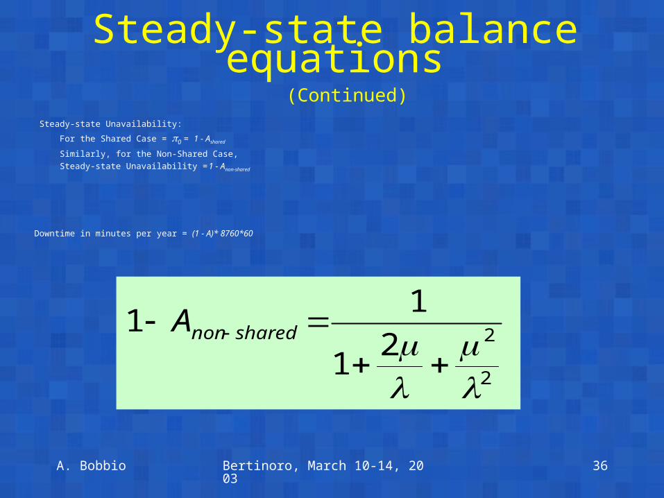
Steady-state balance equations (Continued)
Steady-state Unavailability:
For the Shared Case = 0 = 1 - Ashared
Similarly, for the Non-Shared Case,
Steady-state Unavailability = 1 - Anon-shared
Downtime in minutes per year = (1 - A)* 8760*60
2
221
11
sharednonA
A. Bobbio Bertinoro, March 10-14, 2003 37
Steady-state balance equations
A. Bobbio Bertinoro, March 10-14, 2003 38
Absorbing states MTTF
A. Bobbio Bertinoro, March 10-14, 2003 39
Absorbing states - MTTF
BjidPz jiji
),(,)(0 ,,
jiz ,
Markov Reliability Model with Imperfect Coverage
A. Bobbio Bertinoro, March 10-14, 2003 41
Markov model with imperfect coverage
Next consider a modification of the 2-component parallel system proposed by Arnold as a model of duplex processors of an electronic switching system. We assume that not all faults are recoverable and that c is the coverage factor which denotes the conditional probability that the system recovers given that a fault has occurred. The state diagram is now given by the following picture:
A. Bobbio Bertinoro, March 10-14, 2003 42
Now allow for Imperfect coverage
c
A. Bobbio Bertinoro, March 10-14, 2003 43
Markov modelwith imperfect coverage
Assume that the initial state is 2 so that:
Then the system of differential equations are:
0)0()0(,1)0( 102 PPP
)()()1(2)(
)()()(2)(
)()()1(2)(2)(
120
121
1222
tPtPcdt
tdP
tPtcPdt
tdP
tPtPctcPdt
tdP
A. Bobbio Bertinoro, March 10-14, 2003 44
Markov model with imperfect coverage
)]1([2
)21(
c
cMTTF
After solving the differential equations we obtain:
R(t)=P2(t) + P1(t)
From R(t), we can obtain system MTTF:
It should be clear that the system MTTF and system reliability
are critically dependent on the coverage factor.
A. Bobbio Bertinoro, March 10-14, 2003 45
Source of fault coverage dataMeasurement data from an operational system
Large amount of data neededImproved instrumentation needed
Fault-injection experimentsExpensive but badly neededTools from CMU,Illinois, LAAS (Toulouse)
A fault/error handling submodel (FEHM)Phases: detection, location, retry, reconfig, rebootEstimate duration and probability of success of
each phase
A. Bobbio Bertinoro, March 10-14, 2003 46
Redundant System with Finite Detection Switchover Time
Modify the Markov model with imperfect coverage to allow for finite time to detect as well as imperfect detection.
You will need to add an extra state, say D. The rate at which detection occurs is . Draw the state diagram and investigate the
effects of detection delay on system reliability and mean time to failure.
A. Bobbio Bertinoro, March 10-14, 2003 47
Redundant System with Finite Detection Switchover Time
Assumptions:
Two units have the same MTTF and MTTR;
Single shared repair person;
Average detection/switchover time tsw=1/;
We need to use a Markov model.
A. Bobbio Bertinoro, March 10-14, 2003 48
Redundant System with Finite Detection Switchover Time
11D2 0
2
/1
/1
MTTR
MTTF
A. Bobbio Bertinoro, March 10-14, 2003 49
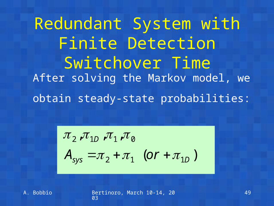
Redundant System with Finite Detection Switchover Time
After solving the Markov model, we obtain
steady-state probabilities:
)(
,,,
112
0112
Dsys
D
orA
A. Bobbio Bertinoro, March 10-14, 2003 50
Closed-form
Er
rA D
/))(2
(2
2
2
112
E
E
E
E
D
1
2
1
)(
1
1
1]2)(
1[
2
2
2
2
1
1
0
2
22
0
A. Bobbio Bertinoro, March 10-14, 2003 51
WFS Example
A. Bobbio Bertinoro, March 10-14, 2003 52
A Workstations-Fileserver Example
Computing system consisting of:– A file-server– Two workstations– Computing network connecting them
System operational as long as:– One of the Workstations
and– The file-server are operational
Computer network is assumed to be fault-free
A. Bobbio Bertinoro, March 10-14, 2003 53
The WFS Example
A. Bobbio Bertinoro, March 10-14, 2003 54
Assuming exponentially distributed times to failure
w : failure rate of workstation
f : failure rate of file-server
Assume that components are repairable
w: repair rate of workstation
f: repair rate of file-server
File-server has priority for repair over workstations (such repair priority cannot be captured by non-state-space models)
Markov Chain for WFS Example
A. Bobbio Bertinoro, March 10-14, 2003 55
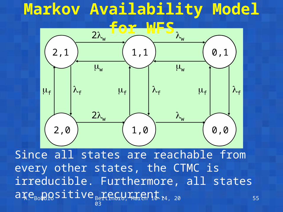
Markov Availability Model for WFS
0,0
2,1 1,1
1,02,0
0,1
f
2w
2w
w
w w
w
f f ff f
Since all states are reachable from every other states, the CTMC is irreducible. Furthermore, all states are positive recurrent.
A. Bobbio Bertinoro, March 10-14, 2003 56
In the figure, the label (i,j) of each state is
interpreted as follows:
i represents the number of workstations that are
still functioning
j is 1 or 0 depending on whether the file-server is
up or down respectively.
Markov Availability Model for WFS (Continued)
A. Bobbio Bertinoro, March 10-14, 2003 57
For the example problem, with the states ordered as (2,1), (2,0), (1,1), (1,0), (0,1), (0,0) the Q matrix is given by:
Markov Availability Model for WFS (Continued)
ff
ffww
wwff
wfwfww
wwff
wfwf
0000
)(000
0)(00
0)(0
0020)2(
0002)2(
Q =
A. Bobbio Bertinoro, March 10-14, 2003 58
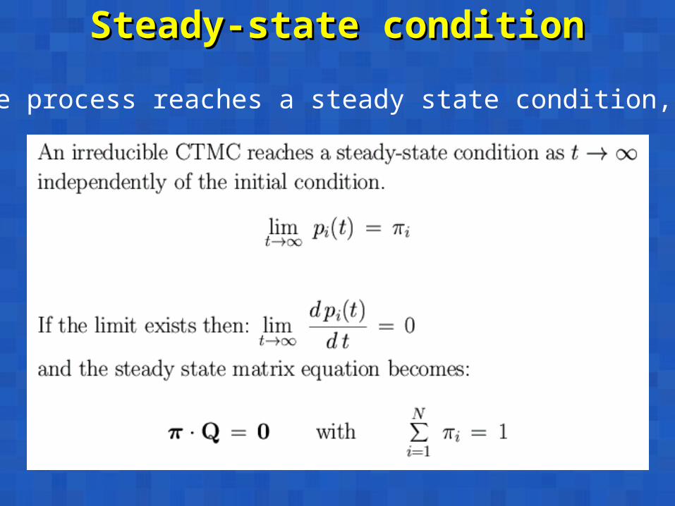
Markov Model (steady-state) : Steady-state probability vector
These are called steady-state balance equations
rate of flow in = rate of flow out
after solving for obtain Steady-state availability
1,0 i
iQ
1121 SSA
),,,,,( 000110112021
,
A. Bobbio Bertinoro, March 10-14, 2003 59
We compute the availability of the system:
System is available as long as it is in states
(2,1) and (1,1).
Instantaneous availability of the system:
Markov Availability Model
sst
AtA
tPtPtA
)(lim
)()()( )1,1()1,2(
A. Bobbio Bertinoro, March 10-14, 2003 60
Markov Availability Model (Continued)
9999.0ssA
1111 5.0,0.1,00005.0,0001.0 hrhrhrhr fwfw
A. Bobbio Bertinoro, March 10-14, 2003 61
Assume that the computer system does not recover if
both workstations fail, or if the file-server fails
Markov Reliability Model with Repair
A. Bobbio Bertinoro, March 10-14, 2003 62
Markov Reliability Model with Repair
States (0,1), (1,0) and (2,0) become absorbing states while (2,1) and (1,1)
are transient states.
Note: we have made a simplification that, once the CTMC reaches a system
failure state, we do not allow any more transitions.
A. Bobbio Bertinoro, March 10-14, 2003 63
Markov Model with Absorbing States
If we solve for P2,1(t) and P1,1(t) then
R(t)=P2,1(t) + P1,1(t)
For a Markov chain with absorbing states: A: the set of absorbing states B = - A: the set of remaining states
zi,j: Mean time spent in state i,j until absorption
BjidPz jiji
),(,)(0 ,,
)0(BB PQz
A. Bobbio Bertinoro, March 10-14, 2003 64
Markov Model with Absorbing States (Continued)
Mean time to absorption MTTA is given as:
Bji
jizMTTA),(
),(
QB derived from Q by restricting it to only states in B
A. Bobbio Bertinoro, March 10-14, 2003 65
Markov Reliability Model with Repair (Continued)
)(
2)2(
wfww
wwfBQ
[ ]
)(2)()(
)()(2solveFirst
1,21,11,1
1,11,21,2
tPtPdt
dP
tPtPdt
dP
wwfw
ww
A. Bobbio Bertinoro, March 10-14, 2003 66
Mean time to failure is 19992 hours.
Markov Reliability Model with Repair (Continued)
1,11,2
1,11,2
1,11,2
1,11,2
:Then
0 )(2
1))2((solvenext
)()()( :Then
zzMTTF
zz
zz
tPtPtR
wfww
wwf
A. Bobbio Bertinoro, March 10-14, 2003 67
Assume that neither workstations nor file-server is repairable
Markov Reliability Model without Repair
A. Bobbio Bertinoro, March 10-14, 2003 68
Markov Reliability Model without Repair (Continued)
States (0,1), (1,0) and (2,0) become absorbing states
A. Bobbio Bertinoro, March 10-14, 2003 69
Mean time to failure is 9333 hours.
Markov Reliability Model without Repair (Continued)


![List of Publications of Andrea Bobbio 1971 1972 1973 1974people.unipmn.it/bobbio/BIBLIO/bliagg.pdf · List of Publications of Andrea Bobbio 1971 [1] ... metodo del rumore di corrente.](https://static.documents.pub/doc/80x56/5b3511ea7f8b9a3a6d8cbea8/list-of-publications-of-andrea-bobbio-1971-1972-1973-list-of-publications-of.jpg)


