A macroscale mixture theory analysis of deposition … macroscale mixture theory analysis of...

The Cryosphere, 9, 1857–1878, 2015

www.the-cryosphere.net/9/1857/2015/

doi:10.5194/tc-9-1857-2015

© Author(s) 2015. CC Attribution 3.0 License.

A macroscale mixture theory analysis of deposition and

sublimation rates during heat and mass transfer in dry snow

A. C. Hansen and W. E. Foslien

Department of Mechanical Engineering, University of Wyoming, Laramie, WY 82071, USA

Correspondence to: A. C. Hansen ([email protected])

Received: 5 February 2015 – Published in The Cryosphere Discuss.: 5 March 2015

Revised: 11 August 2015 – Accepted: 21 August 2015 – Published: 23 September 2015

Abstract. The microstructure of a dry alpine snowpack is

a dynamic environment where microstructural evolution is

driven by seasonal density profiles and weather conditions.

Notably, temperature gradients on the order of 10–20 K m−1,

or larger, are known to produce a faceted snow microstruc-

ture exhibiting little strength. However, while strong temper-

ature gradients are widely accepted as the primary driver for

kinetic growth, they do not fully account for the range of

experimental observations. An additional factor influencing

snow metamorphism is believed to be the rate of mass trans-

fer at the macroscale.

We develop a mixture theory capable of predicting

macroscale deposition and/or sublimation in a snow cover

under temperature gradient conditions. Temperature gradi-

ents and mass exchange are tracked over periods ranging

from 1 to 10 days. Interesting heat and mass transfer behav-

ior is observed near the ground, near the surface, as well as

immediately above and below dense ice crusts. Information

about deposition (condensation) and sublimation rates may

help explain snow metamorphism phenomena that cannot be

accounted for by temperature gradients alone.

The macroscale heat and mass transfer analysis requires

accurate representations of the effective thermal conductiv-

ity and the effective mass diffusion coefficient for snow. We

develop analytical models for these parameters based on first

principles at the microscale. The expressions derived contain

no empirical adjustments, and further, provide self consistent

values for effective thermal conductivity and the effective

diffusion coefficient for the limiting cases of air and solid ice.

The predicted values for these macroscale material parame-

ters are also in excellent agreement with numerical results

based on microscale finite element analyses of representative

volume elements generated from X-ray tomography.

1 Introduction

The thermodynamically active nature of snow, coupled with

unusual high porosities, poses significant challenges to mod-

eling heat and mass transfer in a snow cover. A primary driver

in much of the research on this subject has been efforts to ex-

plain the evolving microstructure of snow that often occurs

in a matter of hours or days. Notably, snow metamorphism,

induced by strong temperature gradients in a snow cover, is

known to produce a highly faceted microstructure, the pres-

ence of which results in extremely weak layers in a snow

cover. Weak layers have been observed near the ground, near

the surface, as well as above and below dense layers (e.g., ice

crusts) within a snow cover.

While strong temperature gradients are widely accepted

as the primary driver in temperature gradient metamor-

phism (TGM), they do not fully account for the range of ex-

perimental observations. For instance, slightly faceted crys-

tal growth has been observed at low temperature gradient

(3 K m−1) where rounded grains from sintering have nor-

mally been observed (Flin and Brzoska, 2008). In contrast,

Pinzer and Schneebeli (2009) note that rounded grain forms

have been observed in surface layers subjected to alternating

temperature gradients of opposite direction.

An additional factor influencing snow metamorphism is

believed to be the rate of mass transfer at the macroscale.

The influence of mass transfer at the macroscale is often

neglected for the simple fact that deposition (condensation)

and sublimation rates caused by vapor diffusion and phase

changes are not known in a typical macroscale analysis.

Vapor diffusion and the associated phase changes at the

macroscale pose modeling challenges in that it forces the

macroscopic analysis toward a mixture theory where the ice

and humid air constituents retain their identity. Mixture the-

Published by Copernicus Publications on behalf of the European Geosciences Union.

1858 A. C. Hansen and W. E. Foslien: A macroscale mixture theory analysis

ory itself is a subject that has yet to fully mature and many

open questions remain.

Implementing a macroscopic continuum mixture theory to

elucidate the coupled heat and mass transfer phenomena oc-

curring in snow is the central focus of this paper. We study

the effects of mass transfer near the ground, near the surface

including diurnal temperature effects, as well as adjacent to

an ice crust within the snow cover. Heat and mass transfer

rates are tracked over several different time periods ranging

up to 10 days.

The mixture theory analysis developed herein requires an

accurate assessment of macroscopic properties for effective

thermal conductivity and the effective mass diffusion coef-

ficient for snow. Determining these parameters requires an

analysis of heat and mass transfer at the microscale. A major

challenge in microstructural studies of snow metamorphism

is the extremely complex 3-D structure of the ice phase.

Historically, generating an accurate geometric representa-

tion of the microstructure of snow and further connecting it

to a subsequent heat and mass transfer analysis was simply

not possible. However, in the last 2 decades, the use of X-ray

computed tomography has profoundly altered experimental

and theoretical research for snow at the microstructural level.

Not only can one accurately capture the true 3-D snow mi-

crostructure, the evolution of the microstructure may be mon-

itored in real time as metamorphism occurs. Furthermore, fi-

nite element analysis may be coupled to experimentally pro-

duced 3-D microstructures to model heat and mass transfer

at the local scale.

High-fidelity microscale numerical models, coupled with

X-ray computer tomography, have been utilized by Riche

and Schneebeli (2013) and Calonne et al. (2011) for pre-

dictions of macroscale effective thermal conductivity. Pinzer

et al. (2012) and Flin and Brzoska (2008) used finite element

analysis with X-ray tomography to address vapor diffusion.

Evolution of the snow microstructure and determining an ef-

fective diffusion coefficient for snow are among their notable

contributions.

Finite element predictions based on computer-generated

X-ray tomography snow structures provide an excellent

foundation for determining material properties for effective

thermal conductivity and the effective diffusion coefficient

for snow. However, instead of utilizing finite element mi-

cromechanics to generate macroscale material properties, we

rely on an interesting mathematical model developed by Fos-

lien (1994). The analytical model produces results for effec-

tive thermal conductivity and the effective diffusion coeffi-

cient for snow that are in remarkable agreement with the

finite element predictions cited above. The model also ac-

counts for effective thermal conductivity and effective dif-

fusion coefficient properties over the entire range of densi-

ties and temperatures possible for snow. The strong corre-

lation of the analytical model material properties compared

with results from microscale finite element analyses of snow

lends confidence to using material parameters based on the

analytical model in the macroscopic mixture theory analysis

developed herein.

2 Reflections on geometric scales: microscale

vs. macroscale variables

The critical heat and mass transfer mechanisms for snow

metamorphism play out at two distinctly different geomet-

ric and time scales. At the microscale (on the order of mil-

limeters) snow exhibits an extremely complex and evolving

microstructure consisting of ice grains and humid air. At the

macroscale, the geometric scale of interest is associated with

the depth of the snow cover – typically on the order of meters.

Macroscopic variables of interest include density, tempera-

ture, temperature gradient, as well as the mass flux of water

vapor and the resulting deposition and sublimation that will

occur within a snow cover. These macroscopic variables are

fundamental drivers for snow structure evolution occurring

at the microscale, thereby coupling local phenomena driving

snow metamorphism with macroscale heat and mass transfer.

When developing a theory that transcends multiple geo-

metric scales, attention must be paid to the transition from

the microscale to the macroscale, commonly referred to as

homogenization. An implicit requirement necessary for ho-

mogenization in an upscale process is appropriate separation

of scales, both from a geometric and physical viewpoint. Au-

riault et al. (2009) provide extensive discussion of necessary

conditions required for separation of scales, all of which are

satisfied for the present work.

A notable aspect of the present homogenization process is

that a mixture theory is introduced by defining snow at the

macroscale to be a mixture composed of an ice constituent

and a humid air constituent. The constituent variables may,

in turn, be appropriately averaged to obtain the macroscale

snow field variables. Allowing the constituents to retain their

identity provides a vehicle to study mass transfer due to con-

densation and sublimation at the macroscale.

As a means of formalizing an upscaling process for snow,

the concept of a representative volume element (RVE) is in-

troduced. The RVE must be of sufficient size such that vol-

ume averages of the constituent variables do not change as

the volume is increased.

Given an RVE, let φα denote the volume fraction of con-

stituent α. The mixture constituents are immiscible, and the

constituent volume fractions are space filling, leading to the

relation

φi+φha = 1, (1)

where subscripts (i) and (ha) denote the ice and humid air

constituents, respectively.

The density of snow, ρ, is defined by the volume aver-

age of the local (microscale) density field, γm(x), that varies

throughout the RVE, i.e.,

The Cryosphere, 9, 1857–1878, 2015 www.the-cryosphere.net/9/1857/2015/

A. C. Hansen and W. E. Foslien: A macroscale mixture theory analysis 1859

ρ =1

V

∫V

γm(x)dV, (2)

where, for clarity, the local density may be expressed as

γm(x)= γiχi(x)+ γha (1−χi(x)) (3)

in terms of the indicator function χi(x) of the ice phase. The

subscript (m) on the local density field is used to emphasize

that the variable is defined at the microscale.

In the case of a mixture, the integral of Eq. (2) may be

broken into an ice domain and a humid air domain as

ρ =1

V

∫Vi

γm(x)dV +1

V

∫Vha

γm(x)dV. (4)

Moreover, the following macroscale constituent densities are

introduced as

γi =1

Vi

∫Vi

γm(x)dV, (5)

and

γha =1

Vha

∫Vha

γm(x)dV. (6)

Noting Eqs. (4)–(6) leads to a volume average expression for

the density of snow given by

ρ = φiγi+φhaγha. (7)

We emphasize that the mixture formulation is defined en-

tirely at the macroscale. Hence, all variables in Eq. (7) repre-

sent macroscale quantities.

Following Özdemir et al. (2008), heat transfer properties

are introduced into the micro–macro upscaling process by

defining the macroscopic heat capacity as(ρCV

)=

1

V

∫V

γm

(CV)

mdV, (8)

where CV is the specific heat at constant volume. This equa-

tion provides a definition for the specific heat of snow yield-

ing consistent values of heat capacity at both scales. Follow-

ing the same development as for the density of snow leads to

the relation(ρCV

)= φi

(γiC

Vi

)+φha

(γhaC

Vha

), (9)

where the heat capacity for constituent α is given by(γαC

Vα

)=

1

Vα

∫Vα

γm

(CV)

mdV. (10)

Özdemir et al. (2008) further enforces consistency of the

stored heat at the microscale and macroscale through the re-

lation

(ρCV

)θ =

1

V

∫V

γm

(CV)

mθmdV, (11)

where θm and θ represent the local temperature and

macroscale temperature, respectively. Again, the integral of

Eq. (11) may be separated into an ice constituent and a humid

air constituent as

(ρCV

)= φi

1

Vi

∫Vi

γm

(CV)

mθmdV

+φha

1

Vha

∫Vha

γm

(CV)

mθmdV

. (12)

Constituent temperatures, θi and θha, are introduced through

the relations

γiCVi θi =

1

Vi

∫Vi

γm

(CV)

mθmdV, (13)

and

γhaCVhaθha =

1

Vha

∫Vha

γm

(CV)

mθmdV. (14)

The heat capacity is heterogeneous at the microscale but ho-

mogeneous in the ice phase, leading to a volume average

temperature for ice given by

θi =1

Vi

∫Vi

θmdV. (15)

For the range of temperatures of interest, the mass fraction

of water vapor in dry air is on the order of 10−3. Hence, the

thermal properties of the humid air may be taken to be those

of dry air, and the heat capacity of dry air is constant for the

temperature variations seen at the microscale. This condition

leads to a volume average definition for the temperature of

the humid air constituent given by

θha =1

Vha

∫Vha

θmdV. (16)

The temperature of snow may be determined from(ρCV

)θ = φi

(γiC

Vi

)θi+φha

(γhaC

Vha

)θha. (17)

Hence, the temperature of snow does not follow the con-

stituent volume averaging found for the heat capacity (Eq. 9)

and the density (Eq. 4) but rather is based on a volume aver-

age weighted by the constituent heat capacities.

The temperature gradient at the microscale is a critical pa-

rameter driving temperature gradient metamorphism. To this

end, volume averaged temperature gradients for the ice and

humid air constituents are introduced as

www.the-cryosphere.net/9/1857/2015/ The Cryosphere, 9, 1857–1878, 2015


– ∇θi ice temperature gradient

– ∇θha humid air temperature gradient

where, for example,

∇θi =1

Vi

∫Vi

∇xθm(x)dV. (18)

The subscript x on the gradient operator in Eq. (18) is used

to emphasize that the gradient applies at the microscale.

Given appropriate boundary conditions for the RVE, the

macroscale temperature gradient for snow satisfies the vol-

ume weighted averaging:

∇θ = φi∇θi+φha∇θha. (19)

Özdemir et al. (2008) develop the specific boundary condi-

tions for the RVE that are necessary to satisfy Eq. (19). These

boundary conditions are precisely the ones used by Pinzer

et al. (2012) and Riche and Schneebeli (2013) in their finite

element analyses of heat and mass transfer at the microscale.

Finally, it is extremely important to recognize differences

in behavior between local (microscale) temperature gradients

and the volume averaged macroscale temperature gradient.

For instance, Pinzer et al. (2012) provide a figure of the local

temperature gradients in an RVE for an applied macroscale

temperature gradient of 50 K m−1. The color bar for the

microscale temperature gradient indicates that local values

of the temperature gradient are as high as 300 K m−1. The

high local values of the temperature gradient compared to

the macroscopic temperature gradient must be kept in mind

when interpreting macroscopic results, as it is the local tem-

perature gradients that drive metamorphism. Hence, when

macroscale temperature gradients are presented as computed

by the mixture theory analysis, it is not unreasonable to as-

sume the microscale temperature gradients may be an order

of magnitude higher in some areas of the RVE.

3 A mixture theory model for macroscale heat and

mass transfer

The common phase changes occurring in snow have moti-

vated several studies using variants of mixture theories. Mor-

land et al. (1990) and Bader and Weilenmann (1992) devel-

oped a four constituent mixture theory for snow where one of

the constituents was water. Phenomena such as percolation,

melting, and freezing are addressed, and momentum balance

plays a significant role in the work. The present work does

not involve momentum balance, nor does it allow for a water

constituent.

Gray and Morland (1994) developed a mixture theory for

dry snow based on constituents of ice and dry air. Their work

is in sharp contrast to the present study where water vapor is

a critical component of the development. Indeed, the empha-

sis of the present work is the prediction of deposition and/or

sublimation of water vapor at the macroscale.

Adams and Brown (1990) studied heat and mass transfer

in snow using a classical form of mixture theory where water

vapor was included. Their work focused on non-equilibrium

conditions of the constituents, whereas the present work is

based on equilibrium of constituent temperatures and a satu-

rated vapor density. Equilibrium vs. non-equilibrium condi-

tions amounts to a focus on different time scales.

Aside from the different areas of emphasis in the study

of phase change phenomena in snow, the mixture theories

cited are based on a classical theory of mixtures, whereas

the present work is largely based on a volume fraction mix-

ture theory (Hansen et al., 1991). The volume fraction theory

produces the same balance equations found in the classical

developments of mixture theory. However, the summed con-

stituent balance equations are not forced to reduce to those

of a single continuum except for the special case of a non-

diffusing mixture. As a result of relaxing this constraint, the

physical definitions of mixture variables as well as the con-

straints on mass, momentum, and energy interaction terms

assume more appealing forms. We rely on the physical argu-

ments of Sect. 2 to define mixture quantities of interest.

Albert and McGilvary (1992) incorporated the effects of

mass diffusion in a heat and mass transfer analysis of snow

centered on forced convection caused by windy conditions

close to the snow surface, a phenomenon known as wind

pumping. The equations developed involve a velocity of the

humid air and conditions where the snow is not assumed to

be saturated with water vapor. These conditions only occur

in snow under extreme circumstances.

Foslien (1994) performed a dimensional analysis of the

conditions needed for convection and showed the Rayleigh

number for typical snow conditions was 1–2 orders of mag-

nitude below what is needed for the onset of convection. As

a consequence, convection is not considered, and the present

paper develops a theory with no air velocity, and further, a

saturated vapor density.

The work of Calonne et al. (2014a) is perhaps the most

closely related to the present work in that they developed the

governing equations for macroscopic heat and water vapor

transfer in dry snow by homogenization involving a multi-

scale expansion. We draw comparisons of their work for the

governing macroscale equations as well as the expressions

for effective thermal conductivity and the effective diffusion

coefficient in snow.

A unique aspect of the present approach is that analyti-

cal models, grounded in first principles at the microscale, are

developed for the effective thermal conductivity and the ef-

fective diffusion coefficient in snow. By starting at the mi-

croscale, albeit with idealized microstructures, we are af-

forded the advantage of using the true thermal conductivities

of ice (ki) and humid air (kha) as well as the known diffu-

sion coefficient of water vapor in air (Dv−a). The resulting



models for the effective thermal conductivity of snow and

the effective diffusion coefficient for snow contain no empir-

ical adjustments and are in remarkable agreement with high-

fidelity numerical predictions of these parameters based on

snow microstructures obtained from X-ray tomography. The

models also generate an analytical description of the separa-

tion of heat transfer due to mass diffusion and heat transfer

due to conduction.

Consistent with the discussion on homogenization, we

consider snow at the macroscale to be a two-constituent mix-

ture consisting of ice and humid air. The humid air itself is

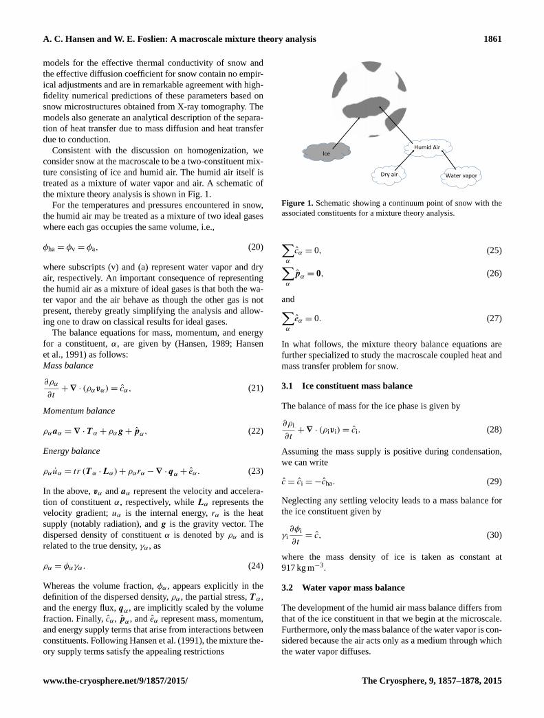
treated as a mixture of water vapor and air. A schematic of

the mixture theory analysis is shown in Fig. 1.

For the temperatures and pressures encountered in snow,

the humid air may be treated as a mixture of two ideal gases

where each gas occupies the same volume, i.e.,

φha = φv = φa, (20)

where subscripts (v) and (a) represent water vapor and dry

air, respectively. An important consequence of representing

the humid air as a mixture of ideal gases is that both the wa-

ter vapor and the air behave as though the other gas is not

present, thereby greatly simplifying the analysis and allow-

ing one to draw on classical results for ideal gases.

The balance equations for mass, momentum, and energy

for a constituent, α, are given by (Hansen, 1989; Hansen

et al., 1991) as follows:

Mass balance

∂ρα

∂t+∇ · (ραvα)= cα, (21)

Momentum balance

ραaα =∇ ·T α + ραg+ pα, (22)

Energy balance

ραuα = tr (T α ·Lα)+ ραrα −∇ · qα + eα. (23)

In the above, vα and aα represent the velocity and accelera-

tion of constituent α, respectively, while Lα represents the

velocity gradient; uα is the internal energy, rα is the heat

supply (notably radiation), and g is the gravity vector. The

dispersed density of constituent α is denoted by ρα and is

related to the true density, γα , as

ρα = φαγα. (24)

Whereas the volume fraction, φα , appears explicitly in the

definition of the dispersed density, ρα , the partial stress, T α ,

and the energy flux, qα , are implicitly scaled by the volume

fraction. Finally, cα , pα , and eα represent mass, momentum,

and energy supply terms that arise from interactions between

constituents. Following Hansen et al. (1991), the mixture the-

ory supply terms satisfy the appealing restrictions

Ice Humid Air

Dry air Water vapor

Figure 1. Schematic showing a continuum point of snow with the

associated constituents for a mixture theory analysis.

∑α

cα = 0, (25)∑α

pα = 0, (26)

and∑α

eα = 0. (27)

In what follows, the mixture theory balance equations are

further specialized to study the macroscale coupled heat and

mass transfer problem for snow.

3.1 Ice constituent mass balance

The balance of mass for the ice phase is given by

∂ρi

∂t+∇ · (ρivi)= ci. (28)

Assuming the mass supply is positive during condensation,

we can write

c = ci =−cha. (29)

Neglecting any settling velocity leads to a mass balance for

the ice constituent given by

γi

∂φi

∂t= c, (30)

where the mass density of ice is taken as constant at

917 kg m−3.

3.2 Water vapor mass balance

The development of the humid air mass balance differs from

that of the ice constituent in that we begin at the microscale.

Furthermore, only the mass balance of the water vapor is con-

sidered because the air acts only as a medium through which

the water vapor diffuses.



Mass transfer of the water vapor may be expressed as (Bird

and Lightfoot, 1960)

γvvv =γv

γha

(γava+ γvvv)+ jv. (31)

Equation (31) says that the mass flux of the water vapor is

due to the bulk fluid motion (the barycentric velocity) plus a

relative velocity due to diffusion. In the absence of a pressure

gradient, the barycentric velocity is zero, i.e.,

γhavha = (γava+ γvvv)= 0. (32)

Mass balance due to diffusion may be expressed in the form

of Fick’s law (Bird and Lightfoot, 1960) as

jv =−γhaDv−a∇x

(γv

γha

), (33)

whereDv−a is the binary diffusion coefficient for water vapor

in air and ∇x denotes the gradient operator at the microscale.

The diffusive flux can be expanded to give

jv =−Dv−a∇xγv+γv

γha

Dv−a∇xγha, (34)

but the second term on the right is negligibly small because

the mass fraction of saturated water vapor in air at 273 K is

about 4× 10−3. Hence, mass transfer of water vapor at the

microscale may be described by

γvvv =−Dv−a∇xγv. (35)

In the transition to the macroscale, the same physical princi-

ples apply but one must now use an effective diffusion coeffi-

cient for water vapor. The need to introduce an effective dif-

fusion coefficient for water vapor is attributed to the presence

of the ice microstructure in snow. Specifically, the presence

of the ice constituent introduces vapor transfer mechanisms

that both enhance and retard mass transfer of water vapor

when compared to a medium of humid air only. These mass

transfer mechanisms are briefly discussed in Sect. 5.3.

Defining Deffs as the effective diffusion coefficient for the

humid air constituent at the macroscale follows

φvγvvv = ρvvv =−Deffs ∇γv, (36)

where vv and γv now represent appropriately volume aver-

aged macroscale variables. Note that the mass flux of wa-

ter vapor is based on the dispersed density, ρv, in order to

account for the reduced volume occupied by the humid air

in the mixture. Finally, since only the humid air constituent

is associated with diffusion in a mixture of ice and humid

air, Deffs also represents the effective diffusion coefficient for

snow.

Again, noting air is simply the medium for mass transfer

of water vapor, the balance of mass for the vapor phase may

be written as

∂ρv

∂t+∇ · (ρvvv)= cv. (37)

Substitution of the diffusive flux into Eq. (37) and noting

cv= cha=−c leads to

∂ρv

∂t−∇ ·

(Deff

s ∇γv

)=−c. (38)

Expanding the time derivative of the dispersed density of the

water vapor gives

∂ρv

∂t= γv

∂φv

∂t+φv

∂γv

∂t, (39)

but

∂φv

∂t=∂φha

∂t=−

∂φi

∂t. (40)

The above results, along with the mass balance for the ice

constituent (Eq. 30), can be used to write Eq. (38) as

φv

∂γv

∂t−∇ ·

(Deff

s ∇γv

)= c

(γv

γi

− 1

), (41)

but the quantityγv

γi� 1. Neglecting this term and noting

φv=φha, the mass balance equation for the water vapor be-

comes

φha

∂γv

∂t−∇ ·

(Deff

s ∇γv

)=−c. (42)

Equation (42) states that changes in the water vapor density

at the macroscale are due to the divergence of the water vapor

flux and sublimation or condensation as defined through the

mass supply.

3.3 Momentum balance

The momentum balance for the ice phase can be used to find

the stress and strain in the ice phase. However, the effect that

the ice stress has on the vapor density of the water is ne-

glected, so the ice phase momentum balance is not consid-

ered further.

The momentum balance for the humid air phase becomes

important when bulk fluid motion occurs as in the case of

convection. Foslien (1994) has shown the Rayleigh number

for a typical snow cover is more than an order of magnitude

below the critical value for the onset of convection, so con-

vection is unlikely to occur except in extreme circumstances.

Therefore, the momentum balance of the humid air phase is

not considered further.

3.4 Ice constituent energy balance

The energy balance for the ice constituent may be expressed

at the macroscale as

ρiui = tr (T i ·Li)+ ρiri−∇ · q i+ ei. (43)



In the above, any velocity gradient in the ice, Li, is attributed

to settling and may be neglected. Moreover, heat generation

from solar radiation is also neglected but could easily be in-

cluded as Colbeck (1989) and McComb et al. (1992) have

done. These assumptions reduce the energy balance for ice

to

ρiui =−∇ · q i+ ei. (44)

The internal energy of the non-deforming ice is assumed to

be a function of temperature only and is given by

ui = CVi (θi− θref) , (45)

where CVi is the specific heat of ice at constant volume

and θref is the reference temperature. The heat flux at the

macroscale is expressed as Fourier’s law of heat conduction

as

q i =−φikeffi ∇θi, (46)

where keffi is the effective thermal conductivity for the ice

phase in snow. This parameter should not be confused with

the thermal conductivity of pure ice (ki) as differences arise

due to the complex microstructural network of the ice phase

in snow. The tortuosity of the ice phase, for example, plays a

role in keffi . The only microstructure where ki and keff

i would

be equal for 1-D heat transfer would be the pore microstruc-

ture discussed in the present paper. In a 3-D analysis of snow,

the two parameters are fundamentally different.

Combining Eqs. (44)–(46), the energy balance for the ice

phase is given by

φiγiCVi

∂θi

∂t=∇ ·

(φik

effi ∇θi

)+ ei. (47)

3.5 Humid air constituent energy balance

As with the ice phase, the work term and the energy source

term of the humid air constituent are neglected, thereby re-

ducing the energy equation to

ρhauha =−∇ · qha+ eha. (48)

The internal energy for the humid air mixture of ideal gases

is given by

γhauha = γaCVa (θha− θref)+ γv

(CV

v (θha− θref)+ usg

), (49)

where usg is the latent heat of sublimation of ice. The above

assumes the reference value of the internal energy of ice was

set to zero as was the case.

The definition for the energy flux vector for a mixture may

be written as (Bird and Lightfoot, 1960)

q = qc+ qd, (50)

where qc is the conductive flux and qd represents a “contri-

bution from the interdiffusion of various species present”. In

the case of a mixture of water vapor and air, the energy flux

is given by

qha =−kha∇xθha+ usgγvvv, (51)

where γv vv, is the mass flux of water vapor diffusing through

air.

Now consider snow at the macroscale composed of a mix-

ture of humid air and ice. At this scale, Eq. (51) must be

modified as

qha =−φhakeffha ∇θha+φhausgγvvv. (52)

The interpretation of the volume fraction in each term on

the right-hand side of the above equation is clear when one

views the energy flux across a surface of a macroscale control

volume of snow. Specifically, the true energy flux of humid

air must be scaled by the area fraction of the humid air at the

control surface. From quantitative stereology, the area frac-

tion is equal to the volume fraction, resulting in Eq. (52).

Noting Eq. (36), mass transfer of the humid air may be

expressed as a diffusive flux, leading to

qha =−φhakeffha ∇θha− usgD

effs ∇γv, (53)

where Deffs represents an effective diffusion coefficient for

snow.

As in the case of the ice phase, one must recognize that keffha

represents an effective thermal conductivity of the humid air

in snow, and this parameter is different from the true thermal

conductivity of humid air as a pure substance. The difference

in the two parameters is again attributed to the complex mi-

crostructure of the humid air phase in snow. In brief, just as

the effective thermal conductivity of snow, keffs is influenced

by microstructure, so are keffi and keff

ha as all three parameters

are macroscale quantities. As such, they depend on a host of

microstructural variables other than temperature.

Substituting Eqs. (49) and (53) into Eq. (48) leads to

φha

(γaC

Va + γvC

Vv

) ∂θha

∂t+ usg

(φha

∂γv

∂t−∇ ·

(Deff

s ∇γv

))=∇ ·

(φhak

effha ∇θha

)+ eha, (54)

but

c =∇ ·

(Deff

s ∇γv

)−φha

∂γv

∂t, (55)

from the mass balance of the water vapor given by Eq. (42).

Therefore, Eq. (54), governing the energy balance of humid

air, assumes the form

φha

(γaC

Va + γvC

Vv

) ∂θha

∂t=∇ ·

(φhak

effha ∇θha

)+ eha+ usgc. (56)

Hence, the change in internal energy for the humid air is at-

tributed to the divergence of the heat flux, energy exchange

with the ice constituent through the energy supply, and en-

ergy exchange through phase changes accounted for by the

mass supply.



4 Separation of scales: macroscale observations

In this section, we discuss some observations that lead to

important simplifications in the macroscale heat and mass

transfer solution. Moreover, we demonstrate separation of

the time scales for local and global heat and mass transfer,

a condition required for homogenization.

4.1 Macroscale temperatures

An important simplification in the analysis of heat and mass

transfer at the macroscale is to assume the constituent tem-

peratures are equal and write

θ = θi = θha,

where θ is the macroscale temperature of snow. Justification

for assuming the ice and humid air temperatures are equal

starts by writing a 1-D heat conduction equation at the mi-

croscale given by

∂θα

∂t=

(kα

γαCVα

)∂2θα

∂x2. (57)

Equation (57) is non-dimensionalized by introducing the fol-

lowing dimensionless variables:

t∗ = t/to, x∗= x/Lc, and θ∗ =

θ − θinit

θf− θinit

.

The resulting non-dimensional equation is

∂θ∗

∂t∗=

(tokα

L2cγαC

Vα

)∂2θ∗

∂x∗2. (58)

The time scale, tmicroo , for heat conduction on the microscale

is introduced as

tmicroo =

γαCVα L

2c

kα. (59)

The time scale, tmacroo , for heat conduction in a snow cover is

similarly defined as

tmacroo =

(φiγiC

Vi +φhaγhaC

Vha

)H 2

keffs

, (60)

whereH is the height of the snowpack and keffs represents the

effective thermal conductivity for snow.

Riche and Schneebeli (2013) provide an expression for the

effective thermal conductivity of snow as a function of snow

density. Assuming a snow density of 200 kg m−3, a depth of

1 m, and a microscale characteristic length of 1 mm, the ra-

tio of the time scale for heat conduction on the macroscale

of the snowpack to the time scale for heat conduction on

the microscale is on the order of 106, which suggests that

macroscale thermal equilibrium between the ice and humid

air constituents is a good assumption. Moreover, the large

separation of scales in the time domain is consistent with the

discussion of Auriault et al. (2009) regarding separation of

time scales necessary for homogenization.

The assumption of uniform constituent temperatures at

the macroscale should not be confused with the local (mi-

croscale) temperature. Under a macroscale temperature gra-

dient, local constituent temperatures in the interior of the

RVE differ due to different thermal conductivities of the ice

and humid air. Further, temperature gradients within individ-

ual constituents are also present at the microscale. A warmer

ice grain is separated from a colder ice grain by pore space,

for example. These temperature differentials drive the mass

transfer process at the microscale. Again, an excellent in-

sight into microscale thermal behavior is provided in Fig. 4

of Pinzer et al. (2012).

Thermal equilibrium of the ice and humid air constituents

at the macroscale allows the constituent energy equations,

(Eqs. 47 and 56), to be added together to yield an energy

equation for snow with a single temperature as

(φhaγhaC

Vha+φiγiC

Vi

) ∂θ∂t=∇ ·

(keff

s ∇θ)+ cusg, (61)

where θ is the temperature of the snow. Notably, the con-

stituent energy supply terms sum to zero in the energy equa-

tion for snow and the volume averaged constituent effective

thermal conductivities have been absorbed into an effective

thermal conductivity for snow, keffs , as

keffs = φik

effi +φhak

effha . (62)

While the effective thermal conductivities, keffi and keff

ha , are

never computed, it would be important to do so if one wanted

to study non-equilibrium constituent temperatures on a short

time scale with a mixture theory.

One can make a direct connection of keffi and keff

ha with

the work of Calonne et al. (2014a). Specifically, the tenso-

rial form of the effective thermal conductivity for snow is

defined in Eq. (25) of Calonne et al. (2014a) as

keffs =

1

|V |

∫V a

ka (∇ta+ I )dV +

∫V i

ki (∇t i+ I )dV

, (63)

where tα characterizes the temperature fluctuation in con-

stituent α and I is the identity tensor.

The above equation may be rearranged as

keffs = φa

1

|Va|

∫V a

ka (∇ta+ I )dV +φi

1

|Vi|

∫V i

ki (∇t i+ I )dV. (64)

Comparing Eqs. (62) and (64) provides a clear mathemat-

ical interpretation of keffi and keff

ha as

keffha =

1

|Va|

∫V a

ka (∇ta+ I )dV, (65)



and

keffi =

1

|Vi|

∫V i

ki (∇t i+ I )dV. (66)

Finally, recent research work has shown the effective ther-

mal conductivity of snow to be anisotropic, see for exam-

ple Schertzer and Adams (2011) and Riche and Schneebeli

(2013). We avoid this complexity at present as it becomes a

non-issue for the 1-D heat and mass transfer theory devel-

oped subsequently.

To summarize, the governing equations for heat and water

vapor transfer in snow are given by Eqs. (42) and (61). These

equations are identical to macroscale equations developed by

Calonne et al. (2014a) through a description at the pore scale

using the homogenization of multiple scale expansions. The

equality is best shown by multiplying the right-hand side of

Eq. (20) in Calonne by (ρi/ρi) and relabeling (Lsg/ρi) as usg,

resulting in Eq. (61) of the present paper. Equation (42) is al-

ready identical in form to Eq. (21) of Calonne et al. (2014a).

While the equations of Foslien (1994) and Calonne et al.

(2014a) governing the macroscale response of heat and mass

transfer in snow are identical, the emphasis of Calonne’s

work is on upscaling, whereas the present paper focuses on

solutions of the macroscale behavior. We also address simi-

larities and differences in the calculation of effective thermal

conductivity and the effective diffusion coefficient for snow,

critical parameters affecting macroscale sublimation and de-

position rates in a snow cover.

4.2 Saturated vapor density at the macroscale

A physical interpretation of the mass supply term, c, is the

mass rate at which water vapor is condensing to form ice per

unit volume of snow. Hobbs (1974) provides an expression

for the condensation of water vapor to ice driven by a differ-

ence in the vapor pressure and the saturated vapor pressure

over ice, (p−psat), as

αcmmol

(p−psat

)(2πmmol�θ)

1/2kgm−2 s−1,

where mmol is the mass per molecule of water, � is Boltz-

man’s constant, and αc is the condensation coefficient.

Multiplying the above expression by the specific surface

area of snow, ξ , and utilizing the ideal gas law for water vapor

provides an explicit expression for the mass supply driven by

a difference in vapor density given by

c =ξRθαcmmol

(γv− γ

satv

)(2πmmol�θ)

1/2. (67)

In the absence of diffusion, Eq. (67) can be combined with

the mass balance equation (Eq. 42) for the water vapor as

φv

∂γv

∂t=ξRθαcmmol

(γv− γ

satv

)(2πmmol�θ)

1/2. (68)

If the saturated vapor density over the ice is held constant,

the time for the vapor density difference between the pore

density and the saturated vapor density to become 0.1 % of

the initial density difference can be computed. Delaney et al.

(1964) measured the condensation coefficient, αc, of ice to

be 0.0144 for temperatures between 271 and 260 K. For a

snow density of 200 kg m−3 and a specific surface area of

1400 m−1, the time for the vapor density in the pore to reach

equilibrium is approximately 1.1× 10−3 s. Hence, the vapor

density in a pore can be assumed to be the saturated vapor

density throughout the process of heat and mass transfer oc-

curring at the macroscale where the time scale of interest is

on the order of hours or days.

The knowledge that the vapor density may be assumed sat-

urated in a macroscale analysis affords a critical simplifica-

tion in the mixture theory analysis in that a constitutive law

for the mass supply is no longer needed. Instead, the mass

supply is computed from Eq. (42) by noting the water vapor

is always saturated at the snow temperature, leading to

c =∇ ·

(Deff

s ∇γ satv

)−φha

∂γ satv

∂t. (69)

We emphasize that Eq. (67) is not utilized in the snowpack

modeling of water vapor deposition and sublimation found

in Sect. 6 as it is replaced by Eq. (69).

4.3 Formulation summary

At this point, we restrict the development to a 1-D model and

write the energy equation, Eq. (61), as

(φhaγhaC

Vha+φiγiC

Vi

) ∂θ∂t=∂

∂x

(keff

s

∂θ

∂x

)+ cusg. (70)

The mass supply equation, Eq. (69), representing phase

changes due to condensation or sublimation assumes the 1-D

form

c =∂

∂x

(Deff

s

∂γ satv

∂x

)−φha

∂γ satv

∂t. (71)

The saturated vapor density may be expressed as purely a

function of temperature (Dorsey, 1968) leading to

∂γ satv

∂x=

dγ satv

dθ

∂θ

∂xand

∂γ satv

∂t=

dγ satv

dθ

∂θ

∂t.

Noting the above, the mass supply equation, Eq. (71), is ex-

pressed as

c =∂

∂x

(Deff

s

dγ satv

dθ

∂θ

∂x

)−φha

dγ satv

dθ

∂θ

∂t. (72)

Finally, substituting Eq. (72) into Eq. (70) leads to a single

partial differential equation governing the energy balance for



snow given by(φhaγhaC

Vha+φiγiC

Vi + usgφha

dγ satv

dθ

)∂θ

∂t

=∂

∂x

(kcon+d

s

∂θ

∂x

), (73)

where

kcon+ds = keff

s + usgDeffs

dγ satv

dθ. (74)

The thermal conductivity kcon+ds is the apparent effective

thermal conductivity of snow that accounts for heat conduc-

tion, keffs , as well as energy transfer due to water vapor diffu-

sion.

Rather than combining Eqs. (70) and (72) and solving

Eq. (73), it is more insightful to solve Eqs. (70) and (72)

separately. Retaining a separate equation for the mass supply

allows one to quantify macroscale deposition and sublima-

tion rates, a fundamental objective of the theory developed

herein.

5 Evaluation of the effective thermal conductivity and

the effective diffusion coefficient for snow

Solution of the energy equation (Eq. 70) and the mass bal-

ance equation (Eq. 72) requires knowledge of macroscale pa-

rameters for effective thermal conductivity as well as the ef-

fective diffusion coefficient for snow. Calonne et al. (2011)

and Riche and Schneebeli (2013) have performed extensive

numerical studies using finite element analysis coupled with

X-ray tomography to quantify the effective thermal conduc-

tivity for snow as a function of density at a fixed temperature.

Calonne et al. (2011) also provide effective thermal conduc-

tivity predictions at two separate temperatures. Pinzer et al.

(2012) and Christon et al. (1994) performed numerical stud-

ies aimed at determining the effective diffusion coefficient

for snow. Calonne et al. (2014a) also used finite element mi-

cromechanics to predict an effective diffusion coefficient for

snow although the specific numerical approach to evaluate

this parameter followed a fundamentally approach.

Regardless of the parameter being studied, a drawback of

microscale finite element analysis (micromechanics) is that

the results provide heat and mass transfer properties at a sin-

gle temperature and density. Hence, a complete characteri-

zation of these parameters as a function of density and tem-

perature requires a significant number of micromechanics so-

lutions at multiple densities and temperatures followed by a

curve-fitting exercise.

Rather than relying on finite element micromechanics so-

lutions, we present an analytical approach developed by Fos-

lien (1994) to predict values for the effective thermal con-

ductivity and the effective diffusion coefficient of snow. Fos-

lien’s model has several attractive features including the fol-

lowing:

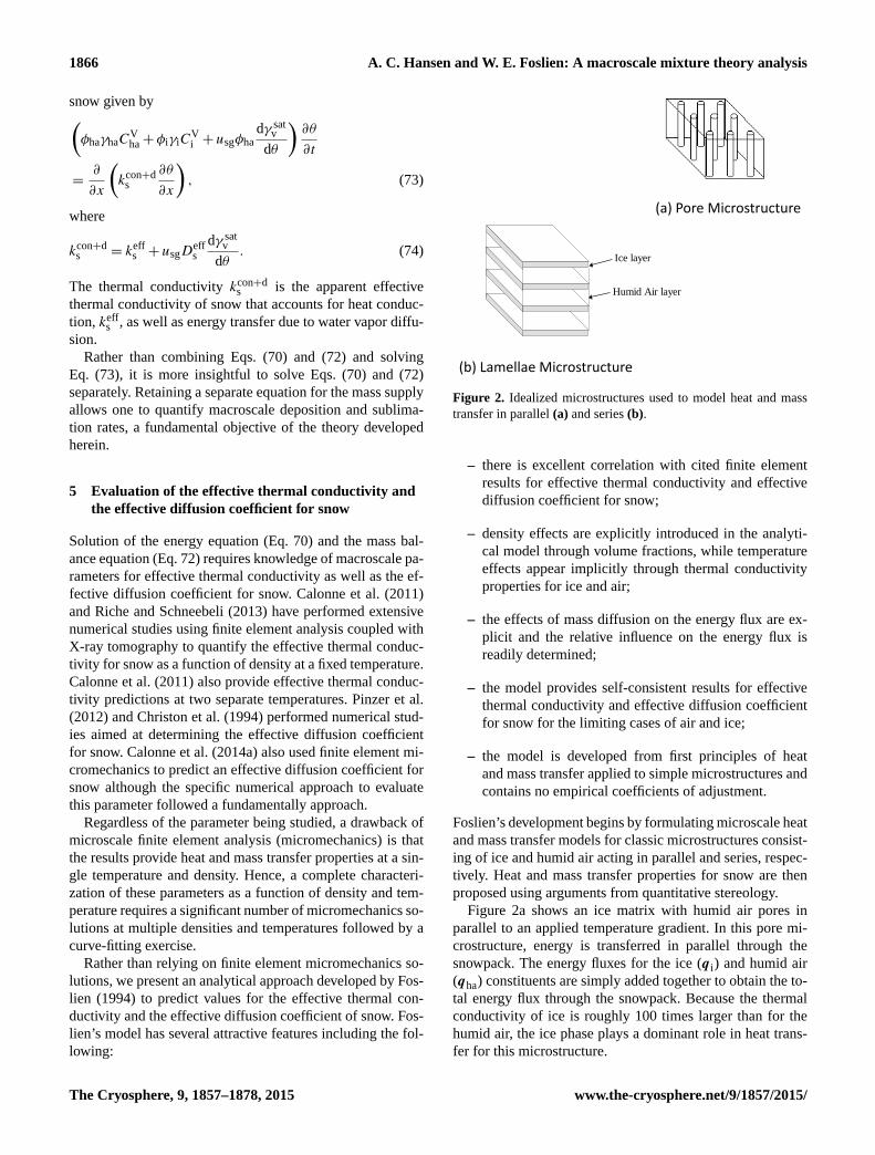
Ice layer

Humid Air layer

(a) Pore Microstructure

(b) Lamellae Microstructure

Figure 2. Idealized microstructures used to model heat and mass

transfer in parallel (a) and series (b).

– there is excellent correlation with cited finite element

results for effective thermal conductivity and effective

diffusion coefficient for snow;

– density effects are explicitly introduced in the analyti-

cal model through volume fractions, while temperature

effects appear implicitly through thermal conductivity

properties for ice and air;

– the effects of mass diffusion on the energy flux are ex-

plicit and the relative influence on the energy flux is

readily determined;

– the model provides self-consistent results for effective

thermal conductivity and effective diffusion coefficient

for snow for the limiting cases of air and ice;

– the model is developed from first principles of heat

and mass transfer applied to simple microstructures and

contains no empirical coefficients of adjustment.

Foslien’s development begins by formulating microscale heat

and mass transfer models for classic microstructures consist-

ing of ice and humid air acting in parallel and series, respec-

tively. Heat and mass transfer properties for snow are then

proposed using arguments from quantitative stereology.

Figure 2a shows an ice matrix with humid air pores in

parallel to an applied temperature gradient. In this pore mi-

crostructure, energy is transferred in parallel through the

snowpack. The energy fluxes for the ice (q i) and humid air

(qha) constituents are simply added together to obtain the to-

tal energy flux through the snowpack. Because the thermal

conductivity of ice is roughly 100 times larger than for the

humid air, the ice phase plays a dominant role in heat trans-

fer for this microstructure.



The second microstructure studied, referred to as a lamel-

lae microstructure, consisted of ice and humid air layers ori-

ented perpendicular to the energy flux (Fig. 2b). In this case,

energy flows in series through the respective layers. Hence,

the energy flux in the humid air constituent must equal the

energy flux through the ice constituent. An interesting fea-

ture of mass transfer in the lamellae microstructure is that

diffusion via the “hand to hand” model described by Yosida

(1955) is naturally present and accounted for in the devel-

opment. Specifically, diffusion is enhanced as the total path

length for diffusion is reduced by the ice layer which acts as

both a source and sink for water vapor.

The two microstructures studied by Foslien (1994) were

first considered by de Quervain (1963) and produce two very

different heat and mass transfer results that are believed to

represent the extremes possible for ice and humid air mix-

tures.

5.1 Pore microstructure

Foslien’s heat and mass transfer analysis of the pore mi-

crostructure begins by writing energy flux expressions for the

ice and humid air constituents at the macroscale. The energy

flux of the ice is attributed to heat conduction, leading to

qi =−ki

∂θ

∂x. (75)

The energy flux of the humid air is attributed to conduction

of the humid air and the mass flux of water vapor. Following

Bird and Lightfoot (1960) we can write

qha =−kha

∂θ

∂x− usgDv−a

dγvsat

dθ

∂θ

∂x. (76)

The energy flux of the pore microstructure is introduced as

qpore =−kpore

∂θ

∂x. (77)

Energy transfer in the pore microstructure occurs in paral-

lel and the energy flux is simply the volume average of the

energy fluxes of the ice and humid air leading to

kpore = φiki+φhakha+φhausgDv−a

dγvsat

dθ. (78)

5.2 Lamellae microstructure

The discontinuous nature of the lamellae microstructure in

the direction of interest introduces a complexity in the spatial

gradients, as the constituent gradients must be defined with

respect to a differential length, dxα . Hence the constituent

energy fluxes assume the form

qi =−ki

∂θ

∂xi

, (79)

and

qha =−kha

∂θ

∂xha

− usgDv−a

dγvsat

dθ

∂θ

∂xha

. (80)

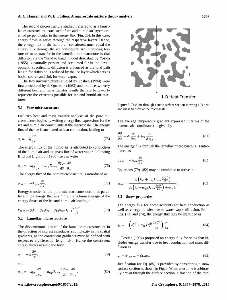
1-D Heat Transfer

Figure 3. Test line through a snow surface section showing 1-D heat

and mass transfer at the microscale.

The average temperature gradient expressed in terms of the

macroscale coordinate x is given by

∂θ

∂x= φi

∂θ

∂xi

+φha

∂θ

∂xha

. (81)

The energy flux through the lamellae microstructure is intro-

duced as

qlam =−klam

∂θ

∂x. (82)

Equations (79)–(82) may be combined to arrive at

klam =

ki

(kha+ usgDv−a

dγ satv

dθ

)φi

(ka+ usgDv−a

dγ satv

dθ

)+φhaki

. (83)

5.3 Snow properties

The energy flux for snow accounts for heat conduction as

well as energy transfer due to water vapor diffusion. From

Eqs. (73) and (74), the energy flux may be identified as

qs =−

(keff

s + usgDeffs

dγ satv

dθ

)∂θ

∂x. (84)

Foslien (1994) proposed an energy flux for snow that in-

cludes energy transfer due to heat conduction and mass dif-

fusion as

qs = φiqpore+φhaqlam. (85)

Justification for Eq. (85) is provided by considering a snow

surface section as shown in Fig. 3. When a test line is arbitrar-

ily drawn through the surface section, a fraction of the total



length will pass through the ice constituent, and the remain-

der will pass through the humid air constituent. If one imag-

ines a 1-D heat transfer occurring along the test line, heat

transfer through the ice phase is dominated by the pore mi-

crostructure where the thermal conductivity of ice is nearly

100 times that of air. In contrast, anytime the test line passes

through the humid air constituent, heat transfer would be

dominated by the lamellae microstructure. Using the lineal

fraction as the weighted behavior of the thermal conduc-

tivity and recognizing the lineal fraction is identical to the

volume fraction under conditions of isotropy (Underwood,

1970) leads directly to Eq. (85).

Combining Eqs. (77)–(78) and Eqs. (82)–(83) with

Eq. (85) leads to an expression for the energy flux of snow

given by

qs =−

φi (φhakha+φiki)+φha

kikha

φi

(kha+ usgDv−a

dγ satv

dθ

)+φhaki

∂θ

∂x−

φi (φhaDv−a)+φha

kiDv−a

φi

(kha+ usgDv−−a

dγ satv

dθ

)+φhaki

usgdγ sat

v

dθ

∂θ

∂x. (86)

Motivated by the functional forms of Eqs. (84) and (86),

we define the effective thermal conductivity and effective dif-

fusion coefficient as

keffs =φi (φhakha+φiki)+φha kikha

φi

(kha+ usgDv−a

dγ satv

dθ

)+φhaki

, (87)

and

Deffs =φi (φhaDv−a)+φha kiDv−a

φi

(kha+ usgDv−a

dγ satv

dθ

)+φhaki

. (88)

Despite the presence of the binary diffusion coefficient of

water vapor in air in the expression for keffs , it should be em-

phasized that the result given in Eq. (87) represents the effec-

tive thermal conductivity for snow as predicted by the ana-

lytical model. Similarly, constituent thermal conductivity pa-

rameters appear in the equation for the effective diffusion co-

efficient of snow, Deffs . These results are a consequence of a

direct application of heat and mass transfer principles for the

lamellae microstructure – the parameters of thermal conduc-

tivity and diffusion simply do not separate at the macroscale

for this microstructure.

A good deal of clarity in the physical interpretation of keffs

and Deffs may be achieved through an order of magnitude

analysis of the various terms in Eqs. (87) and (88). To be-

gin, for the range of temperatures of interest, one may show

kha and (usgDv−adγ sat

v

dθ) are of the same order of magnitude.

Now rearrange Eqs. (87) and (88) by dividing numerator and

denominator of the last term in each by ki, leading to

keffs = φi (φhakha+φiki)+φha

kha

φi

[kha+usgDv−a

dγ satv

dθki

]+φha

, (89)

and

Deffs = φi (φhaDv−a)+φha

Dv−a

φi

[kha+usgDv−a

dγ satv

dθ

ki

]+φha

.(90)

The value of the thermal conductivity of ice is on the order

of 100 times that of the term (kha+ usgDv−adγ sat

v

dθ). There-

fore, neglecting the term in square brackets in the above ex-

pressions for keffs and Deff

s leads to

keffs = φi (φhakha+φiki)+ kha, (91)

and

Deffs = φiφhaDv−a+Dv−a. (92)

Equations (91) and (92) reveal a desirable consistency

in terms. Specifically, the effective thermal conductivity of

snow depends only on the thermal conductivities of ice and

humid air, respectively, while the effective diffusion coeffi-

cient for snow depends only on the binary coefficient of wa-

ter vapor in air. Hence, the thermal conductivity and diffusion

expressions decouple from one another.

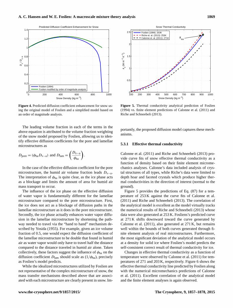
Owing to the “clean” nature of the simplified forms for keffs

andDeffs , one might be tempted to use them at all times. That

approach is, indeed, valid for the effective thermal conduc-

tivity as the simplified effective thermal conductivity curve

is nearly identical to the original proposed by Foslien. How-

ever, important differences arise in the diffusion predictions.

Figure 4 shows the effective diffusion curves predicted by

Eqs. (88) and (92), respectively. The two curves are iden-

tical over a wide range of densities from approximately 0

to 400 kg m−3. As the curves deviate at higher densities, the

original form proposed by Foslien is necessary to drive Deffs

to the known limiting value of zero for solid ice. The consis-

tency of Foslien’s model is impressive in this regard.

There is yet another physically pleasing aspect of Foslien’s

model for the effective diffusion coefficient for snow. Using

the simplified form of Eq. (92), one can write the effective

diffusion coefficient as

Deffs = φi (φhaDv−a)+φha

(Dv−a

φha

). (93)



0 200 400 600 800 10000

0.2

0.4

0.6

0.8

1

1.2

1.4

Snow Density (kg m−3)

Ds /

Dv−

a

Predicted Diffusion Coefficient Enhancement for Snow

Foslien (1994)Foslien modified by order of magnitude analysis

Figure 4. Predicted diffusion coefficient enhancement for snow us-

ing the original model of Foslien and a simplified model based on

an order of magnitude analysis.

The leading volume fraction in each of the terms in the

above equation is attributed to the volume fraction weighting

of the snow model proposed by Foslien, allowing us to iden-

tify effective diffusion coefficients for the pore and lamellae

microstructures as

Dpore = (φhaDv−a) and Dlam =

(Dv−a

φha

).

In the case of the effective diffusion coefficient for the pore

microstructure, the humid air volume fraction leads Dv−a.

The interpretation of φha is quite clear, as the ice phase acts

as a blockage and limits the amount of area for humid air

mass transport to occur.

The influence of the ice phase on the effective diffusion

of water vapor is fundamentally different for the lamellae

microstructure compared to the pore microstructure. First,

the ice does not act as a blockage of diffusion paths in the

lamellae microstructure as it does in the pore microstructure.

Secondly, the ice phase actually enhances water vapor diffu-

sion in the lamellae microstructure by shortening the path-

way needed to travel via the “hand to hand” mechanism de-

scribed by Yosida (1955). For example, given an ice volume

fraction of 0.5, one would expect the diffusion coefficient of

the lamellae microstructure to be double that found in humid

air as water vapor would only have to travel half the distance

compared to the distance traveled in humid air alone. Taken

collectively, these factors suggest the influence of φha on the

diffusion coefficient Dlam should scale as (1/φha), precisely

as Foslien’s model predicts.

While the idealized microstructures utilized by Foslien are

not representative of the complex microstructure of snow, the

mass transfer mechanisms described above that are associ-

ated with each microstructure are clearly present in snow. Im-

100 200 300 400 500 600 700 800 900 10000

0.5

1

1.5

2

2.5


k s (W

m−

1 K−

1 )

Snow Thermal Conductivity

kice

Foslien (1994): 253KRiche et. al. (2013): 253KCalonne et. al. (2011): 271K

.

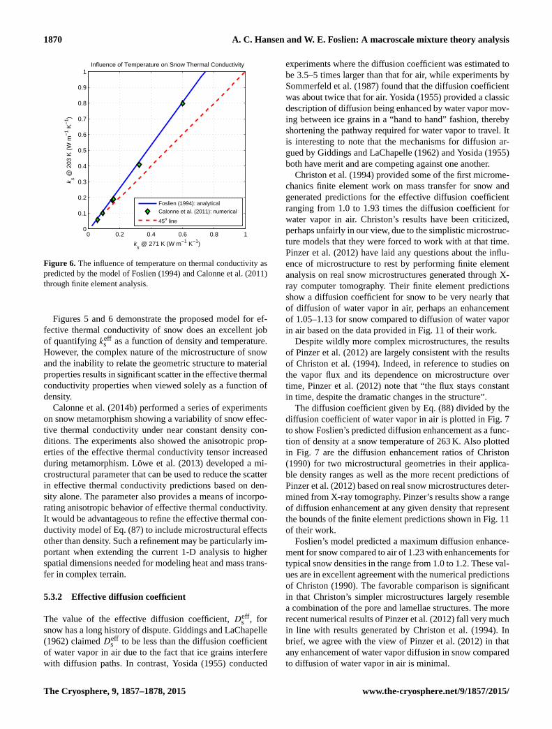
Figure 5. Thermal conductivity analytical prediction of Foslien

(1994) vs. finite element predictions of Calonne et al. (2011) and

Riche and Schneebeli (2013).

portantly, the proposed diffusion model captures these mech-

anisms.

5.3.1 Effective thermal conductivity

Calonne et al. (2011) and Riche and Schneebeli (2013) pro-

vide curve fits of snow effective thermal conductivity as a

function of density based on their finite element microme-

chanics analyses. Calonne’s data included analysis of crys-

tal structures of all types, while Riche’s data were limited to

depth hoar and faceted crystals which produce higher ther-

mal conductivities in the direction of interest (normal to the

ground).

Figure 5 provides the predictions of Eq. (87) for a tem-

perature of 253 K against the curve fits of Calonne et al.

(2011) and Riche and Schneebeli (2013). The correlation of

the analytical model is excellent as the model virtually tracks

the numerical results of Riche and Schneebeli (2013) whose

data were also generated at 253 K. Fosliens’s predicted curve

at 271 K shifts downward toward the curve generated by

Calonne et al. (2011), also generated at 271 K, but remains

well within the bounds of both curves generated through fi-

nite element analysis of real microstructures. Furthermore,

the most significant deviation of the analytical model occurs

at a density for solid ice where Foslien’s model predicts the

self-consistent correct result of thermal conductivity for ice.

Changes in effective thermal conductivity as a function of

temperature were observed by Calonne et al. (2011) for tem-

peratures of 271 and 203 K, respectively. Figure 6 shows the

effective thermal conductivity line predicted by Foslien along

with the numerical micromechanics predictions of Calonne

et al. (2011). Excellent correlation of the analytical model

and the finite element analyses is again observed.



0 0.2 0.4 0.6 0.8 10

0.1

0.2

0.3

0.4

0.5

0.6

0.7

0.8

0.9

1

ks @ 271 K (W m−1 K−1)

k s @ 2

03 K

(W

m−

1 K−

1 )Influence of Temperature on Snow Thermal Conductivity

Foslien (1994): analytical

Calonne et al. (2011): numerical

45o line

Figure 6. The influence of temperature on thermal conductivity as

predicted by the model of Foslien (1994) and Calonne et al. (2011)

through finite element analysis.

Figures 5 and 6 demonstrate the proposed model for ef-

fective thermal conductivity of snow does an excellent job

of quantifying keffs as a function of density and temperature.

However, the complex nature of the microstructure of snow

and the inability to relate the geometric structure to material

properties results in significant scatter in the effective thermal

conductivity properties when viewed solely as a function of

density.

Calonne et al. (2014b) performed a series of experiments

on snow metamorphism showing a variability of snow effec-

tive thermal conductivity under near constant density con-

ditions. The experiments also showed the anisotropic prop-

erties of the effective thermal conductivity tensor increased

during metamorphism. Löwe et al. (2013) developed a mi-

crostructural parameter that can be used to reduce the scatter

in effective thermal conductivity predictions based on den-

sity alone. The parameter also provides a means of incorpo-

rating anisotropic behavior of effective thermal conductivity.

It would be advantageous to refine the effective thermal con-

ductivity model of Eq. (87) to include microstructural effects

other than density. Such a refinement may be particularly im-

portant when extending the current 1-D analysis to higher

spatial dimensions needed for modeling heat and mass trans-

fer in complex terrain.

5.3.2 Effective diffusion coefficient

The value of the effective diffusion coefficient, Deffs , for

snow has a long history of dispute. Giddings and LaChapelle

(1962) claimed Deffs to be less than the diffusion coefficient

of water vapor in air due to the fact that ice grains interfere

with diffusion paths. In contrast, Yosida (1955) conducted

experiments where the diffusion coefficient was estimated to

be 3.5–5 times larger than that for air, while experiments by

Sommerfeld et al. (1987) found that the diffusion coefficient

was about twice that for air. Yosida (1955) provided a classic

description of diffusion being enhanced by water vapor mov-

ing between ice grains in a “hand to hand” fashion, thereby

shortening the pathway required for water vapor to travel. It

is interesting to note that the mechanisms for diffusion ar-

gued by Giddings and LaChapelle (1962) and Yosida (1955)

both have merit and are competing against one another.

Christon et al. (1994) provided some of the first microme-

chanics finite element work on mass transfer for snow and

generated predictions for the effective diffusion coefficient

ranging from 1.0 to 1.93 times the diffusion coefficient for

water vapor in air. Christon’s results have been criticized,

perhaps unfairly in our view, due to the simplistic microstruc-

ture models that they were forced to work with at that time.

Pinzer et al. (2012) have laid any questions about the influ-

ence of microstructure to rest by performing finite element

analysis on real snow microstructures generated through X-

ray computer tomography. Their finite element predictions

show a diffusion coefficient for snow to be very nearly that

of diffusion of water vapor in air, perhaps an enhancement

of 1.05–1.13 for snow compared to diffusion of water vapor

in air based on the data provided in Fig. 11 of their work.

Despite wildly more complex microstructures, the results

of Pinzer et al. (2012) are largely consistent with the results

of Christon et al. (1994). Indeed, in reference to studies on

the vapor flux and its dependence on microstructure over

time, Pinzer et al. (2012) note that “the flux stays constant

in time, despite the dramatic changes in the structure”.

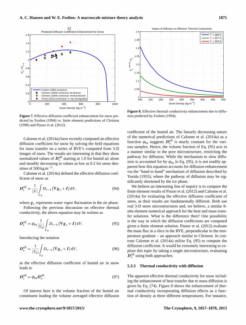
The diffusion coefficient given by Eq. (88) divided by the

diffusion coefficient of water vapor in air is plotted in Fig. 7

to show Foslien’s predicted diffusion enhancement as a func-

tion of density at a snow temperature of 263 K. Also plotted

in Fig. 7 are the diffusion enhancement ratios of Christon

(1990) for two microstructural geometries in their applica-

ble density ranges as well as the more recent predictions of

Pinzer et al. (2012) based on real snow microstructures deter-

mined from X-ray tomography. Pinzer’s results show a range

of diffusion enhancement at any given density that represent

the bounds of the finite element predictions shown in Fig. 11

of their work.

Foslien’s model predicted a maximum diffusion enhance-

ment for snow compared to air of 1.23 with enhancements for

typical snow densities in the range from 1.0 to 1.2. These val-

ues are in excellent agreement with the numerical predictions

of Christon (1990). The favorable comparison is significant

in that Christon’s simpler microstructures largely resemble

a combination of the pore and lamellae structures. The more

recent numerical results of Pinzer et al. (2012) fall very much

in line with results generated by Christon et al. (1994). In

brief, we agree with the view of Pinzer et al. (2012) in that

any enhancement of water vapor diffusion in snow compared

to diffusion of water vapor in air is minimal.



t[]

0 200 400 600 800 10000

0.2

0.4

0.6

0.8

1

1.2

1.4

1.6


Ds /

Dv−

a

Predicted Diffusion Coefficient Enhancement for Snow

Foslien (1994) analyticalChriston (1994) numerical: No BranchChriston (1994) numerical: Vertical BranchPinzer (2012) numerical: X−ray tomography

Figure 7. Effective diffusion coefficient enhancement for snow pre-

dicted by Foslien (1994) vs. finite element predictions of Christon

(1990) and Pinzer et al. (2012).

Calonne et al. (2014a) have recently computed an effective

diffusion coefficient for snow by solving the field equations

for mass transfer on a series of RVE’s computed from 3-D

images of snow. The results are interesting in that they show

normalized values of Deffs starting at 1.0 for humid air alone

and steadily decreasing to values as low as 0.2 for snow den-

sities of 500 kg m−3.

Calonne et al. (2014a) defined the effective diffusion coef-

ficient of snow as

Deffs =

1

|V |

∫V a

Dv−a

(∇gv+ I

)dV, (94)

where gv represents water vapor fluctuation in the air phase.

Following the previous discussion on effective thermal

conductivity, the above equation may be written as

Deffs = φha

1

|Va|

∫V a

Dv−a

(∇gv+ I

)dV. (95)

Introducing the notation

Deffa =

1

|Va|

∫V a

Dv−a

(∇gv+ I

)dV, (96)

as the effective diffusion coefficient of humid air in snow

leads to

Deffs = φhaD

effa . (97)

Of interest here is the volume fraction of the humid air

constituent leading the volume averaged effective diffusion

100 150 200 250 300 350 400 450 5001

1.05

1.1

1.15

1.2

1.25

1.3

1.35

1.4


k s con+

d / k s

Impact of Diffusion on Effective Thermal Conductivity

T = 268 KT = 257 KT = 243 K

Figure 8. Effective thermal conductivity enhancement due to diffu-

sion predicted by Foslien (1994).

coefficient of the humid air. The linearly decreasing nature

of the numerical predictions of Calonne et al. (2014a) as a

function φha suggests Deffa is nearly constant for the vari-

ous samples. Hence, the volume fraction of Eq. (95) acts in

a manner similar to the pore microstructure, restricting the

pathway for diffusion. While the mechanism to slow diffu-

sion is accounted for by φha in Eq. (95), it is not readily ap-

parent how this equation accounts for diffusion enhancement

via the “hand to hand” mechanism of diffusion described by

Yosida (1955), where the pathway of diffusion may be sig-

nificantly shortened by the ice phase.

We believe an interesting line of inquiry is to compare the

finite element results of Pinzer et al. (2012) and Calonne et al.

(2014a) for evaluating the effective diffusion coefficient of

snow, as their results are fundamentally different. Both use

real 3-D snow microstructures and, we believe, a similar fi-

nite element numerical approach for the heat and mass trans-

fer solutions. What is the difference then? One possibility

is the way in which the diffusion coefficients are computed

given a finite element solution. Pinzer et al. (2012) evaluate

the mass flux in a slice in the RVE, perpendicular to the tem-

perature gradient – an approach similar to Christon. In con-

trast Calonne et al. (2014a) utilize Eq. (95) to compute the

diffusion coefficient. It would be extremely interesting to ex-

plore this topic by taking a single microstructure, evaluating

Deffs using both approaches.

5.3.3 Thermal conductivity with diffusion

The apparent effective thermal conductivity for snow includ-

ing the enhancement of heat transfer due to mass diffusion is

given by Eq. (74). Figure 8 shows the enhancement of ther-

mal conductivity incorporating diffusion effects as a func-

tion of density at three different temperatures. For instance,



at a density of 250 kg m−3, the heat transfer enhancement

due to diffusion is 9 and 3 % for temperatures of 268 and

257 K, respectively. These values are reasonably consistent

with calculated values provided by Riche and Schneebeli

(2013) showing latent heat transfer contributions to be ap-

proximately 14 and 1 % for temperatures of 268 and 257 K,

respectively. Specific densities were not provided for the cal-

culations of Riche and Schneebeli (2013) but the average

density of their samples was 254 kg m−3.

The analytical predictions of Foslien shown in Fig. 8 sug-

gest the importance of latent heat transfer by diffusion is

most prominent in low density snow at temperatures near

freezing. In this case, the enhancement of heat transfer due

to diffusion may be as high as 30–40 % for low density snow.

These results are consistent with the numerical studies of

Christon et al. (1994) who note that “the enhancement due

to the transport of latent energy is seen to peak at about 40 %

of the conduction for the lowest density and the highest base

temperature”.

In closing, results from the analytical model for the ther-

mal conductivity of snow, keffs , and the effective diffusion co-

efficient for snow, Deffs , proposed by Foslien are in excellent

agreement with cited finite element micromechanics analy-

ses and, further, the parameter predictions are self-consistent

with the limiting cases of air and solid ice. The results lend

confidence to using the predicted parameters for keffs andDeff

s

over the entire spectrum of temperatures and densities en-

countered in the macroscale heat and mass transfer analyses

presented in Sect. 6.

6 Numerical results for macroscale heat and mass

transfer

In this section, numerical results of the nonlinear equations

(Eqs. 70 and 72) governing heat and mass transfer in a snow-

pack are presented. The specific problem at hand is to model

the heat and mass transfer in a 1 m deep snow cover with

complexities associated with a real snowpack such as dense

layers and a time varying surface boundary condition for

temperature. A Galerkin finite element method was used to

discretize the spatial domain, and the Crank–Nicholson time

integration method is used to advance the solution in time.

The code used to generate the results of Sect. 6.1 is provided

in the Supplement.

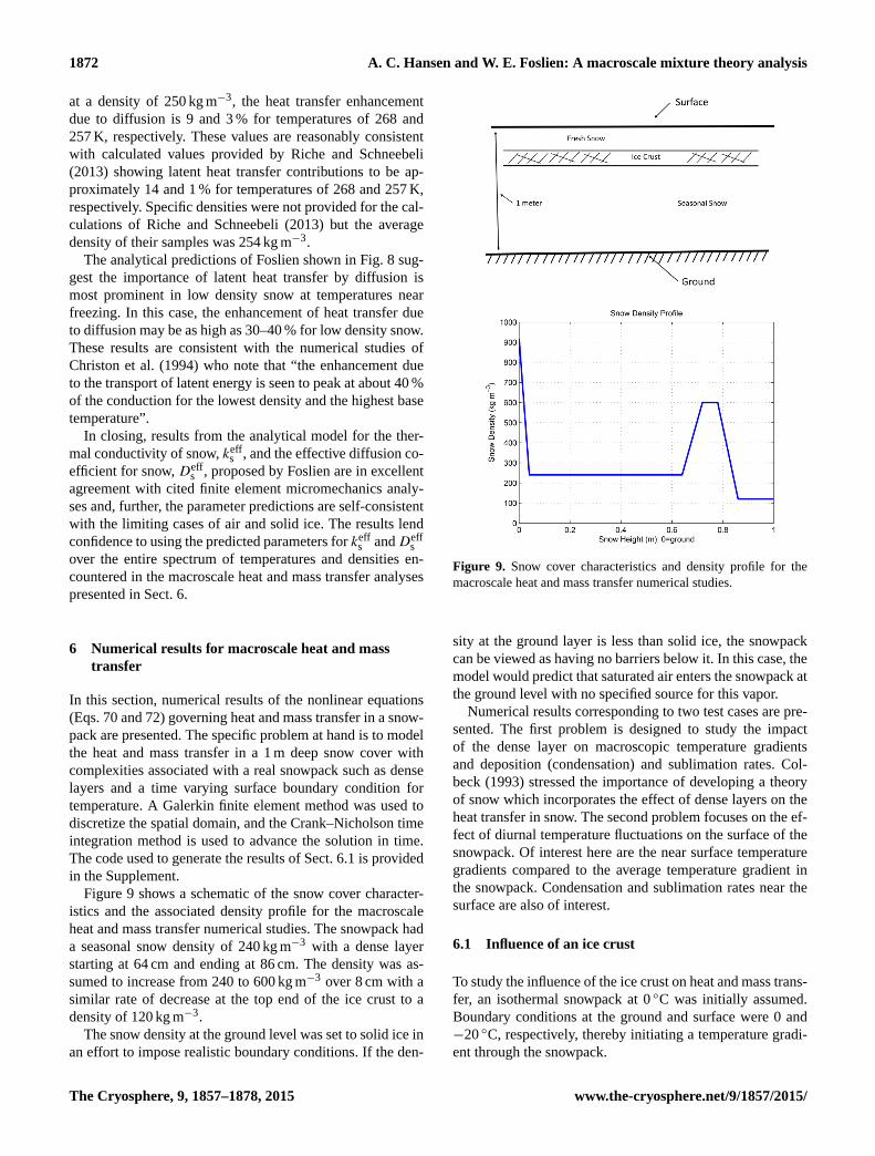
Figure 9 shows a schematic of the snow cover character-

istics and the associated density profile for the macroscale

heat and mass transfer numerical studies. The snowpack had

a seasonal snow density of 240 kg m−3 with a dense layer

starting at 64 cm and ending at 86 cm. The density was as-

sumed to increase from 240 to 600 kg m−3 over 8 cm with a

similar rate of decrease at the top end of the ice crust to a

density of 120 kg m−3.

The snow density at the ground level was set to solid ice in

an effort to impose realistic boundary conditions. If the den-

Figure 9. Snow cover characteristics and density profile for the

macroscale heat and mass transfer numerical studies.

sity at the ground layer is less than solid ice, the snowpack

can be viewed as having no barriers below it. In this case, the

model would predict that saturated air enters the snowpack at

the ground level with no specified source for this vapor.

Numerical results corresponding to two test cases are pre-

sented. The first problem is designed to study the impact

of the dense layer on macroscopic temperature gradients

and deposition (condensation) and sublimation rates. Col-

beck (1993) stressed the importance of developing a theory

of snow which incorporates the effect of dense layers on the

heat transfer in snow. The second problem focuses on the ef-

fect of diurnal temperature fluctuations on the surface of the

snowpack. Of interest here are the near surface temperature

gradients compared to the average temperature gradient in

the snowpack. Condensation and sublimation rates near the

surface are also of interest.

6.1 Influence of an ice crust

To study the influence of the ice crust on heat and mass trans-

fer, an isothermal snowpack at 0 ◦C was initially assumed.

Boundary conditions at the ground and surface were 0 and

−20 ◦C, respectively, thereby initiating a temperature gradi-

ent through the snowpack.



0 0.2 0.4 0.6 0.8 1−20

−18

−16

−14

−12

−10

−8

−6

−4

−2

0

Snow Height (m): 0=ground

Tem

pera

ture

( o C

)

Temperature Profile

1 Day5 Days10 Days

Figure 10. Snowpack temperature profile at 1, 5, and 10 days, re-

spectively.

Figure 10 shows the temperature profile in the snowpack

after 1, 5, and 10 days, respectively. In the dense layer of

snow, the temperature gradient is noticeably reduced at any

time due to the higher thermal conductivity of the dense

snow. The dense layer also has the effect of producing a

much higher temperature gradient in the near surface fresh

snow cover in the pack. Figure 11 shows that, even after

10 days, the temperature gradient near the surface is approx-

imately 60 ◦C m−1, three times the average temperature gra-

dient. The high temperature gradients near the surface are

even more notable when one considers the significant ampli-

fication of temperature gradients that occur at the microscale

as discussed in Sect. 2 and demonstrated in Fig. 4 of Pinzer

et al. (2012).

Figure 12 shows both condensation and sublimation occur-

ring in the snowpack with significant activity near the dense

ice crust. Near the surface, condensation is occurring because

water vapor is diffusing toward the surface which is colder

and, therefore, an area of lower saturation for the vapor den-

sity. The water vapor must then condense if the air is not to

become supersaturated. Just below the dense layer, Fig. 12

shows another area of condensation near the dense ice crust.

Condensation occurs here due to the decrease in humid air

volume fraction in the direction of the water vapor diffusion.

If the amount of air available to hold water decreases, then

the amount of water vapor must also decrease. Just above the

dense layer, the opposite is true. Here, Fig. 12 shows that

sublimation is occurring because the vapor volume fraction

is increasing in the direction of vapor flow. Sublimation must

occur to keep the increasing amount of air saturated.

Local weakening above and below dense layers in a snow

cover have been observed (Adams and Brown, 1982). If con-

densation is known to enhance depth hoar growth (Colbeck,

1983), then the condensation occurring below the dense layer

0 0.2 0.4 0.6 0.8 1−120

−100

−80

−60

−40

−20

0


Tem

pera

ture

Gra

dien

t ( o C

m−

1 )

Temperature Gradient Profile

1 Day5 Days10 Days

Figure 11. Snowpack temperature gradient profile at 1, 5, and

10 days, respectively.

0 0.2 0.4 0.6 0.8 1−16

−14

−12

−10

−8

−6

−4

−2

0

2

4


Mas

s S

uppl

y (m

g m

−3 s

−1 )

Condensation Rate

1 Day5 Days10 Days

Figure 12. Snowpack condensation rates at 1, 5, and 10 days, re-

spectively. Positive values indicate condensation while negative val-

ues indicate sublimation.

in Fig. 12 could contribute to the weakening observed in

this region of a snowpack. Temperature gradients are rela-

tively low below the ice crust, although in the range of where

faceted crystal growth has been observed in field studies. The

sublimation occurring above the dense layer may contribute

to any snowpack weakness observed here.

Sublimation is also observed near the ground after 10 days

and appears to be increasing with time. At a sublimation

rate of 4 mg m−3 s−1 occurring just above the ground af-

ter 10 days, a decrease in density of 1 kg m−3 would take

about 3 days. This slow rate of change in density is consis-

tent with experimental studies on temperature gradient meta-

morphism, where little change in density is observed despite



0.5 0.6 0.7 0.8 0.9 1−30

−25

−20

−15

−10

−5

0


Tem

pera

ture

( o C

)

Temperature Profile

6 Hours12 Hours18 Hours24 Hours

Figure 13. Snowpack temperatures over a 24 h period with time

dependent surface boundary conditions given by Eq. (98).

the dramatic changes in the crystal structure of snow (Pinzer

et al., 2012).

6.2 Effect of diurnal temperatures

To study diurnal temperature effects, the surface of the snow-

pack was subjected to a harmonic temperature boundary con-

dition given by

θ(1, t)=−20− 10sinπt

43 200, (98)

with the lower surface temperature held fixed at 0 ◦C. The

boundary condition given by Eq. (98) has a mean value

of −20 ◦C with a 10 ◦C fluctuation about the mean. Ini-

tial conditions for the temperature through the snowpack

were specified based on the average temperature gradient of

−20 ◦C m−1 at time t = 0.

Figure 13 shows the temperature profile over a 24 h period

at day 5, after any transients have disappeared. Only the up-

per half meter of the snowpack is shown. Strong temperature

gradients are observed in the fresh snow near the surface,

with gradients as high as −150 ◦C m−1 as shown in Fig. 14.

The large temperature gradients found near the surface are

also accompanied by active condensation and sublimation

throughout a 24 h cycle (Fig. 15). Both the temperature gra-

dient and the mass exchange are likely to impact microstruc-

tural changes that occur in the near surface snow cover.

7 Summary

We have developed a macroscale mixture theory analysis for

modeling condensation and sublimation rates in a snow cover

under temperature gradient conditions. The theory is general

enough to accommodate arbitrary density profiles with any

0.5 0.6 0.7 0.8 0.9 1−150

−100

−50

0

50

100


Tem

pera

ture

Gra

dien

t ( o C

m−

1 )

Temperature Gradient Profile


Figure 14. Snowpack temperature gradients over a 24 h period with

time dependent surface boundary conditions given by Eq. (98).

desired time dependent surface boundary conditions. Con-

densation and/or sublimation is observed near the ground and

the surface as well as immediately above and below dense

layers such as ice crusts. Macroscale temperature gradients

can be surprisingly high compared to the average tempera-

ture gradient in the snowpack.

A quantitatively correct macroscale analysis of constituent

mass exchange brings out an interesting microscale analysis

problem that is worthy of attention. Recent numerical studies

of heat and mass transfer at the microscale begin by solving

the steady state diffusion equation for heat transfer with the

appropriate thermal properties of ice and humid air. Dirich-

let boundary conditions for temperature are specified at the

top and bottom of the RVE to simulate a desired tempera-

ture gradient. Once the local temperature field is determined,

a solution for mass transport is obtained for the humid air

phase. The vapor density boundary conditions are specified

at the ice/air interface by assuming the vapor density is satu-

rated, thereby a function of temperature only. Therefore, the

mass flux in such an analysis is essentially dictated by the

macroscale temperature gradient.

The mixture theory results for macroscale deposition and

or sublimation tell an entirely different story. For example,

consider the effects of diurnal temperatures on heat and mass

transfer near the surface as seen in Figs. 14 and 15. Figure 14

shows strong negative temperature gradients at 6 and 24 h

between x= 0.9 m and x= 1.0 m (the region bounded by the

ice crust and the surface). Now, examine Fig. 15 showing

mass exchange at the same time periods and snow depth. The

6 h plot shows deposition is occurring while the 24 h plot

shows sublimation is occurring. The boundary conditions

used for microscale analyses of an RVE described above can-

not capture this interesting phenomenon as the results are

driven by temperature gradient only.



0.5 0.6 0.7 0.8 0.9 1−6

−4

−2

0

2

4

6


Mas

s S

uppl

y (m

g m

−3 s

−1 )

Condensation Rate


Figure 15. Snowpack condensation rates over a 24 h period based

on the diurnal boundary condition of Eq. (98). Positive values indi-

cate condensation while negative values indicate sublimation.

The divergent behavior of macroscale deposi-

tion/sublimation phenomena from the macroscale tem-

perature gradient should come as no surprise from the

mixture theory analysis. Indeed, the ability to show this

phenomenon is the fundamental driver for developing a

mixture theory to begin with. If this were not the case, one

could simply generate a thermal profile from the energy

equation and move on.

Given the mixture theory results described above, it would

be interesting to investigate a transient microscale (RVE) so-

lution exploring the effects of imposing mass flux boundary

conditions for the vapor while using the saturated vapor den-

sity (based on the temperature field) as an initial condition

for the humid air. Perhaps such an analysis could help ex-

plain microstructural evolution (kinetic growth vs. sintering)

under conditions where specifying the temperature gradient

alone is unable to do so. Christon (1990) developed a fully

coupled heat and mass transfer formulation, although bound-

ary conditions involved temperature and temperature gradi-

ent only.

Knowledge of the condensation or sublimation rates at the

macroscale provides the foundation for a fully coupled so-

lution of heat and mass transfer at the microscale. In this

spirit, the mixture theory for snow can simulate interesting

macroscale problems featuring terrain changes, ice crusts,

surface effects, snow storm deposition, extreme tempera-

tures, etc. Heat and mass transfer results from a mixture the-

ory analysis could then be used as inputs for a host of inter-

esting microstructural studies.

Finally, analytical expressions of thermal conductivity and

the effective diffusion coefficient for snow were motivated

from simple microstructures whose heat and mass transfer

are grounded in first principles. The equations developed pro-

vide an elegant path to modeling thermal conductivity and

the effective diffusion coefficient of snow that are needed for

the macroscale mixture theory analysis.



Appendix A

Table A1. Nomenclature.

Latin letters

pα Momentum supply of constituent α (N m−3)

cα Mass supply of constituent α (kg m−3 s−1)

eα Energy supply of constituent α (W m−3)

aα Acceleration of constituent α (m s−2)

g Gravity vector (m s−2)

jv Diffusive flux of water vapor (kg m−2 s−1)

I Identity tensor

V Volume (m3)

Lα Velocity gradient tensor of constituent α (s−1)

uα Specific internal energy of constituent α (J kg−1)

usg Latent heat of sublimation of ice (J kg−1)

rα Heat supply of constituent α (W kg−1)

T α Partial stress tensor of constituent α (Pa)

mmol Mass of a water molecule (kg)

x Position vector (m)

R Water vapor gas constant (J kg−1 K−1)

p Vapor pressure (Pa)

to Time scale (s)

Lo Length scale (m)

H Snowpack height (m)

vα Velocity of constituent α (m s−1)

vv Velocity of water vapor component (m s−1)

va Velocity of air component (m s−1)

CV Specific heat of snow at constant volume (J kg−1 K−1)

CVα Specific heat of constituent α at constant volume (J kg−1 K−1)

Dv−a Diffusion coefficient of water vapor in air (m2 s−1)

Deffs Effective diffusion coefficient of snow (m2 s−1)

Defflam

Effective diffusion coefficient of lamellae microstructure (m2 s−1)

Deffpore Effective diffusion coefficient of pore microstructure (m2 s−1)

kα Thermal conductivity of constituent α (W m−1 K−1)

keffα Effective thermal conductivity of constituent α (W m−1 K−1)

keffs Effective thermal conductivity of snow (W m−1 K−1)

kpore Apparent effective thermal conductivity of pore microstructure including mass diffusion effects (W m−1 K−1)

klam Apparent effective thermal conductivity of lamellae microstructure including mass diffusion effects (W m−1 K−1)

kcon+ds Apparent effective thermal conductivity of snow including mass diffusion effects (W m−1 K−1)

q Energy flux (W m−2)

qα Energy flux of constituent α (W m−2)

qc Energy flux due to conduction (W m−2)

qd Energy flux due to interdiffusion of species (W m−2)

qs Energy flux of snow (W m−2)

t i Vector characterizing temperature fluctuation in the ice phase

ta Vector characterizing temperature fluctuation in the air phase

gv Vector characterizing water vapor density fluctuation in the air phase

ρ Snow density (kg m−3)

γα True density of constituent α – as opposed to a dispersed density (kg m−3)

ρα Dispersed density of constituent alpha (kg m−3)

φα Volume fraction of constituent α

θinit Initial temperature (K)

θfinal Final temperature (K)

θ Temperature (K)

θα Temperature of constituent α (K)

θref Reference temperature (K)



Table A1. Continued.

Greek symbols

χi Indicator function for the ice constituent

αc Condensation coefficient

� Boltzman’s constant (J K−1 molecule−1)

ξ Specific surface area of snow (m−1)

Subscripts

α Arbitrary constituent

a Air component

ha Humid air constituent

i Ice constituent

s Snow

v Water vapor component

m Indicates variable applies at the microscale

ref Reference

Superscripts

eff Effective – applies at the macroscale

sat Saturated water vapor in air∗ Dimensionless variable

Operators

∇ Gradient operator

∇x Gradient operator applied at the microscale



The Supplement related to this article is available online

at doi:10.5194/tc-9-1857-2015-supplement.

Edited by: M. Schneebeli

References

Adams, E. and Brown, R.: Further results on studies of temperature

gradient metamorphism, J. Glaciol., 28, 205–209, 1982.

Adams, E. and Brown, R.: A mixture theory for evaluating heat and

mass transport processes in nonhomogeneous snow, Continuum

Mech. Therm., 2, 31–63, 1990.

Albert, M. R. and McGilvary, W. R.: Thermal effects due to air flow

and vapor transport in dry snowl, J. Glaciol., 38, 273–281, 1992.

Auriault, J.-L., Boution, C., and Geindreau, C.: Homogenization of

Coupled Phenomena in Heterogeneous Media, John Wiley and

Sons, London, 2009.

Bader, H. P. and Weilenmann, P.: Modeling temperature distribu-

tion, energy and mass flow in a (phase-changing) snowpack,

I. Model and case studies, Cold Reg. Sci. Technol., 20, 157–181,

doi:10.1016/0165-232X(92)90015-M, 1992.

Bird, R. B., Stewart, W. E., and Lightfoot, E.: Transport Phenom-

ena, John Wiley and Sons, New York, 1960.

Calonne, N., Flin, F., Morin, S., Lesaffre, B., Roscoat, R., and Gein-

dreau, C.: Numerical and experimental investigations of the ef-

fective thermal conductivity of snow, Geophys. Res. Lett., 38,

L23501, doi:10.1029/2011GL049234, 2011.

Calonne, N., Geindreau, C., and Flin, F.: Macroscopic modeling for

heat and water vapor transport in dry snow by homogenization,

J. Phys. Chem. B, 118, 13393–13403, doi:10.1021/jp5052535,

2014a.

Calonne, N., Flin, F., Geindreau, C., Lesaffre, B., and Rolland du

Roscoat, S.: Study of a temperatue gradient metamorphism of

snow from 3-D images: time evolution of microstructures, phys-

ical properties and their associated anisotrpy, The Cryosphere, 8,

2255–2274, doi:10.5194/tc-8-2255-2014, 2014b.

Christon, M.: 3-D transient microanalysis of multi-phase heat and

mass transfer in ice lattices, PhD thesis, Colorado State Univer-

sity, Fort Collins, CO, USA, 1990.

Christon, M., Burns, P., and Sommerfeld, R.: Quasi-steady tempera-

ture gradient metamorphism in idealized, dry snow, Numer. Heat

Tr. A-Appl., 25, 259–278, doi:10.1080/10407789408955948,

1994.

Colbeck, S.: Theory of metamorphism of dry snow, J. Geophys.

Res., 88, 5475–5482, 1983.

Colbeck, S.: Snow-crystal growth with varying surface temepera-

tures and radiation penetration, J. Glaciol., 35, 23–29, 1989.

Colbeck, S.: The vapor diffusion coefficient for snow, Water Resour.

Res., 29, 109–115, 1993.

Delaney, L. J., Houston, R. W., and Eagleton, L. C.: The rate of

vaporization of water and ice, Chem. Eng. Sci., 19, 105–114,

doi:10.1016/0009-2509(64)85115-0, 1964.

de Quervain, M.: On the metomorphosis of snow, Water Resour.

Res., 29, 109–115, 1963.

Dorsey, N.: Properties of Ordinary Water-Substance, Hafner, New

York, 1968.

Flin, F. and Brzoska, J.: The temperature-gradient metamorphism

of snow: vapour diffusion model and application to tomographic

images, Ann. Glaciol., 49, 17–21, 2008.

Foslien, W.: A modern mixture theory applied to heat and mass

transfer in snow, MS thesis, University of Wyoming, Laramie,

WY, USA, 1994.

Giddings, J. and LaChapelle, W.: The formation rate of depth hoar,

J. Geophys. Res., 67, 2377–2383, 1962.

Gray, J. M. and Morland L. W.: A dry snowpack model, Cold Reg.

Sci. Technol., 22, 135–148, doi:10.1016/0165-232X(94)90025-

6, 1994.

Hansen, A.: Reexamining some basic definitions of modern mix-

ture theory, Int. J. Eng. Sci., 27, 1531–1544, doi:10.1016/0020-

7225(89)90146-8, 1989.

Hansen, A., Damson, M., Donovan, R., Horning, D., and Walker, J.:

Some notes on a volume fraction mixture theory and a compari-

son with the kinetice theory of gases, Int. J. Eng. Sci., 29, 561–

573, doi:10.1016/0020-7225(91)90061-7, 1991.

Hobbs, P.: Ice Physics, Clarendon Press, Oxford, 1974.

Löwe, H. R., Riche, F., and Schneebeli, M.: A general treat-

ment of snow microstructure exemplified by an improved rela-

tion for thermal conductivity, The Cryosphere, 7, 1473–1480,

doi:10.5194/tc-7-1473-2013, 2013.

McComb, T., Rimmer, A., Rodgers, M., Turver, K., and Vickers, A.:

A mathematical model for the prediction of temperature in a dry

snow layer, Cold Reg. Sci. Technol., 20, 247–259, 1992.

Morland, L. W., Kelly, R. J., and Morris, E. M.: A mixture theory for

a phase changing snowpack, Cold Reg. Sci. Technol., 17, 271–

285, doi:10.1016/S0165-232X(05)80006-0, 1990.

Özdemir, W., Brekelmans, A., and Geers, M. G. D.: Computational

homogenization for heat conduction in heterogeneous solids, Int.

J. Numer. Meth. Eng., 73, 185–204, 2008.

Pinzer, B. and Schneebeli, M.: Snow metamorphism under al-

ternating temperature gradients: morphology and recrystal-

ization in surface snow, Geophys. Res. Lett., 36, L23503,

doi:10.1029/2009GL039618, 2009.

Pinzer, B. R., Schneebeli, M., and Kaempfer, T. U.: Vapor flux

and recrystallization during dry snow metamorphism under a

steady temperature gradient as observed by time-lapse micro-

tomography, The Cryosphere, 6, 1141–1155, doi:10.5194/tc-6-

1141-2012, 2012.

Riche, F. and Schneebeli, M.: Thermal conductivity of snow mea-

sured by three independent methods and anisotropy considera-

tions, The Cryosphere, 7, 217–227, doi:10.5194/tc-7-217-2013,

2013.

Schertzer, R. and Adams, E.: Anisotropic thermal conductivity

model for dry snow, Cold Reg. Sci. Technol., 69, 122–128, 2011.

Sommerfeld, R., Friedman, I., and Nilles, M.: The fractionation of

natural isotopes during temperature gradient metamorphism of

snow, in: The Fractionation of Natural Isotopes During Temper-

ature Gradient Metamorphism of Snow, D. Reidel Publishing,

Boston, 95–105, 1987.

Underwood, E.: Quantitative Stereology, Addison-Wesley, Reading,

Mass., USA, 1970.

Yosida, Z.: Physical studies of deposited snow: thermal properties I,

Tech. rep., Institute of low temperature science, Hokkaido Uni-

versity, Japan, 1955.


http://dx.doi.org/10.5194/tc-9-1857-2015-supplement

http://dx.doi.org/10.1016/0165-232X(92)90015-M

http://dx.doi.org/10.1029/2011GL049234

http://dx.doi.org/10.1021/jp5052535

http://dx.doi.org/10.5194/tc-8-2255-2014

http://dx.doi.org/10.1080/10407789408955948

http://dx.doi.org/10.1016/0009-2509(64)85115-0

http://dx.doi.org/10.1016/0165-232X(94)90025-6

http://dx.doi.org/10.1016/0165-232X(94)90025-6

http://dx.doi.org/10.1016/0020-7225(89)90146-8

http://dx.doi.org/10.1016/0020-7225(89)90146-8

http://dx.doi.org/10.1016/0020-7225(91)90061-7

http://dx.doi.org/10.5194/tc-7-1473-2013

http://dx.doi.org/10.1016/S0165-232X(05)80006-0

http://dx.doi.org/10.1029/2009GL039618

http://dx.doi.org/10.5194/tc-6-1141-2012

http://dx.doi.org/10.5194/tc-6-1141-2012

http://dx.doi.org/10.5194/tc-7-217-2013

Date post:	01-May-2018
Category:	Documents
Upload:	vuongbao
View:	220 times
Download:	1 times

A macroscale mixture theory analysis of deposition … macroscale mixture theory analysis of...

Documents