88
Chapter 15 Goodwin, Graebe , Salgado © , Prentice Hall 20 Chapter 15 SISO Controller SISO Controller Parameterizations Parameterizations
| Date post: | 19-Dec-2015 |
| Category: |
Documents |
| View: | 218 times |
| Download: | 1 times |
Chapter 15 Goodwin, Graebe, Salgado©
, Prentice Hall 2000
Chapter 15
SISO Controller SISO Controller ParameterizationsParameterizations
Chapter 15 Goodwin, Graebe, Salgado©
, Prentice Hall 2000
This chapter treats a novel way of expressing a control transfer function.
We will see that this novel parameterization leads to deep insights into control system design and reinforces, from an alternative perspective, many of the ideas that we have previously studied.
The key feature of the new parameterization is that it renders the closed loop sensitivity functions linear (or more correctly, affine) in a design variable. We thus call this the affine parameterization.
Chapter 15 Goodwin, Graebe, Salgado©
, Prentice Hall 2000
The main ideas presented include motivation for the affine parameterization and the idea of
open loop inversion
affine parameterization and Internal Model Control
affine parameterization and performance specifications
PID synthesis using the affine parameterization
control of time delayed plants and affine parameterization. Connections with the Smith controller
interpolation to remove undesirable open loop poles.
Chapter 15 Goodwin, Graebe, Salgado©
, Prentice Hall 2000
Open Loop Inversion Revisited
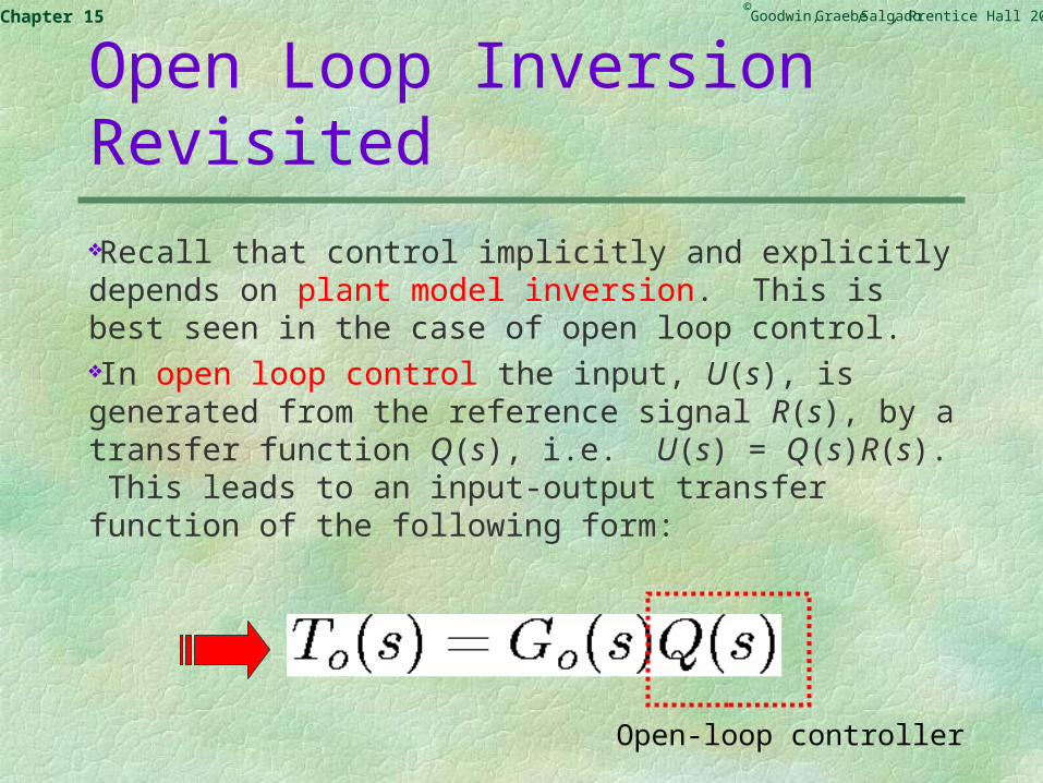
Recall that control implicitly and explicitly depends on plant model inversion. This is best seen in the case of open loop control.In open loop control the input, U(s), is generated from the reference signal R(s), by a transfer function Q(s), i.e. U(s) = Q(s)R(s). This leads to an input-output transfer function of the following form:
Open-loop controller
Chapter 15 Goodwin, Graebe, Salgado©
, Prentice Hall 2000
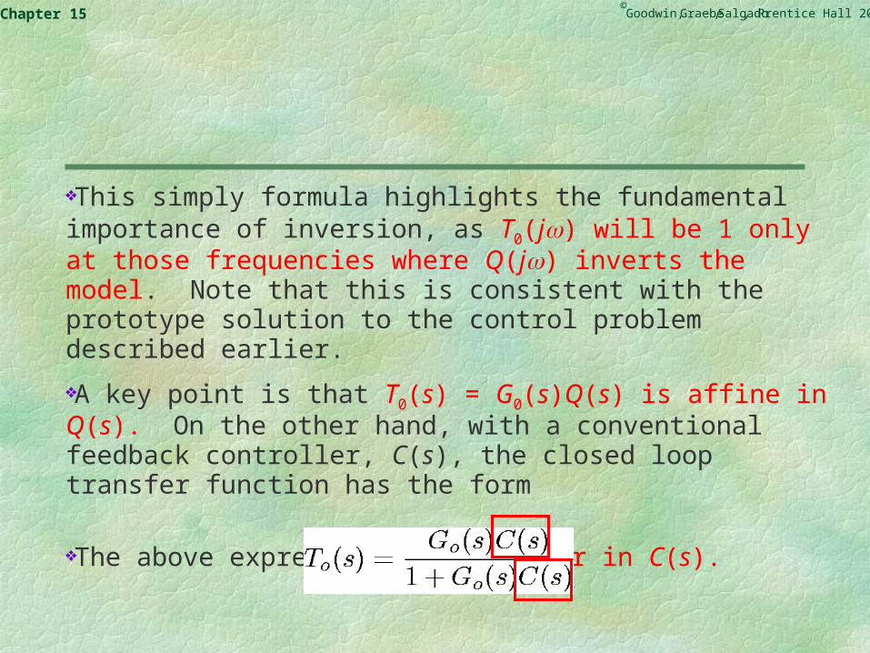
This simply formula highlights the fundamental importance of inversion, as T0(j) will be 1 only at those frequencies where Q(j) inverts the model. Note that this is consistent with the prototype solution to the control problem described earlier.
A key point is that T0(s) = G0(s)Q(s) is affine in Q(s). On the other hand, with a conventional feedback controller, C(s), the closed loop transfer function has the form
The above expression is nonlinear in C(s).
Chapter 15 Goodwin, Graebe, Salgado©
, Prentice Hall 2000
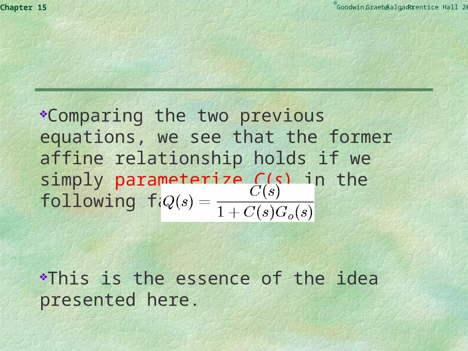
Comparing the two previous equations, we see that the former affine relationship holds if we simply parameterize C(s) in the following fashion:
This is the essence of the idea presented here.
Chapter 15 Goodwin, Graebe, Salgado©
, Prentice Hall 2000
Affine Parameterization. The Stable Case
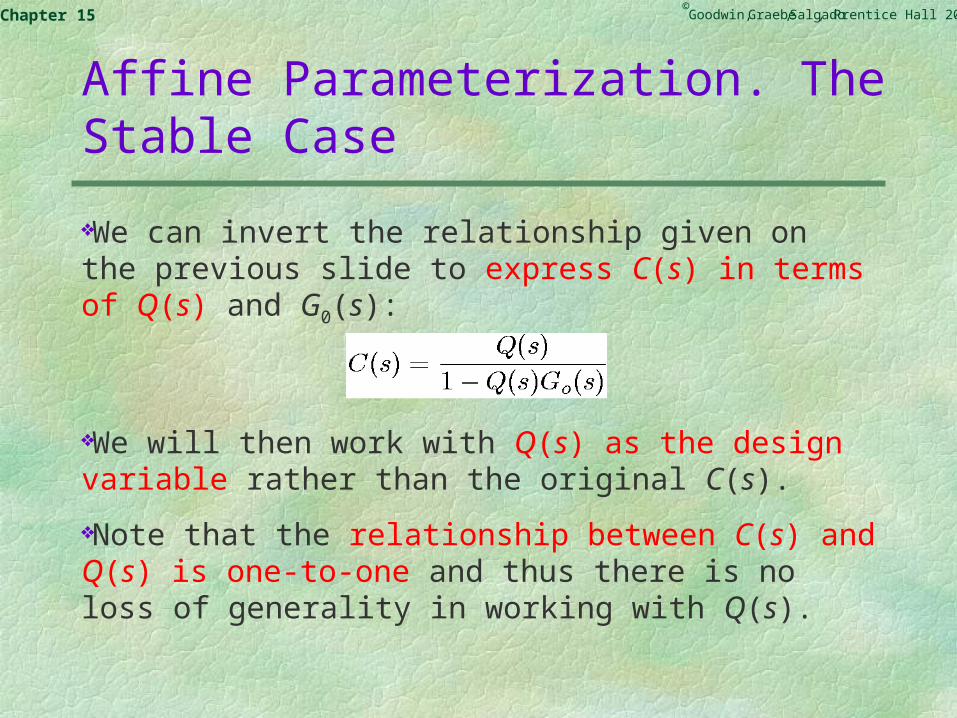
We can invert the relationship given on the previous slide to express C(s) in terms of Q(s) and G0(s):
We will then work with Q(s) as the design variable rather than the original C(s).
Note that the relationship between C(s) and Q(s) is one-to-one and thus there is no loss of generality in working with Q(s).
Chapter 15 Goodwin, Graebe, Salgado©
, Prentice Hall 2000
Stability
Actually a very hard question is the following: “Given a stable transfer function G0(s), describe all controllers, C(s) that stabilize this nominal plant”.
However, it turns out that, in the Q(s) form, this question has a very simple answer, namely all that is required is that Q(s) be stable.
This result is formalized in the lemma stated on the next slide.
Chapter 15 Goodwin, Graebe, Salgado©
, Prentice Hall 2000
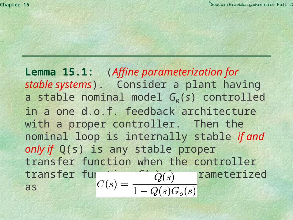
Lemma 15.1: (Affine parameterization for stable systems). Consider a plant having a stable nominal model G0(s) controlled in a one d.o.f. feedback architecture with a proper controller. Then the nominal loop is internally stable if and only if Q(s) is any stable proper transfer function when the controller transfer function C(s) is parameterized as
Chapter 15 Goodwin, Graebe, Salgado©
, Prentice Hall 2000
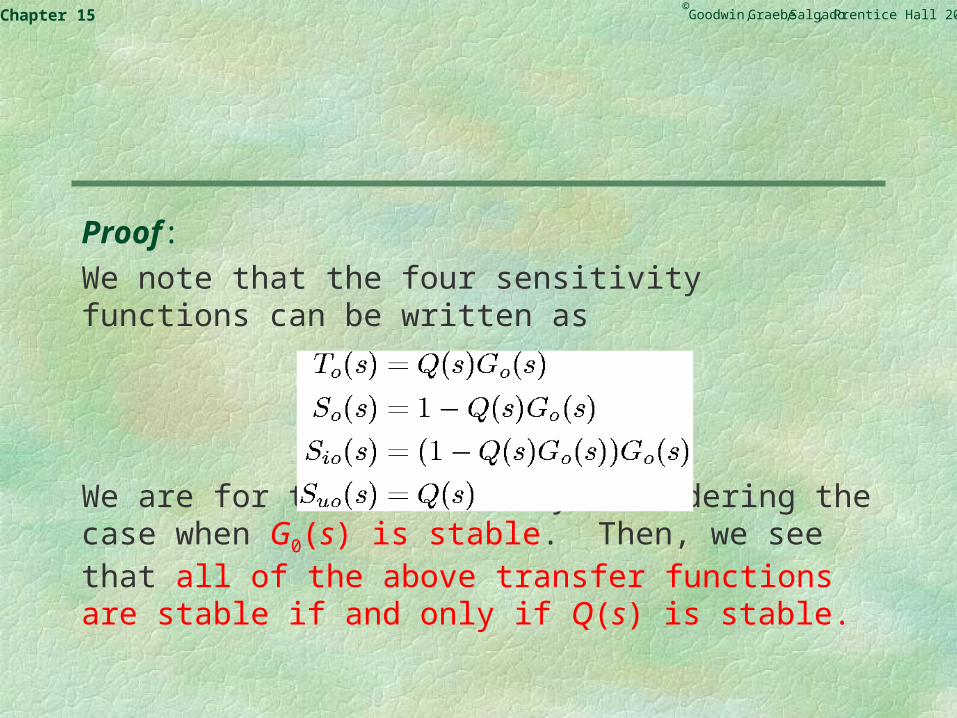
Proof:
We note that the four sensitivity functions can be written as
We are for the moment only considering the case when G0(s) is stable. Then, we see that all of the above transfer functions are stable if and only if Q(s) is stable.
Chapter 15 Goodwin, Graebe, Salgado©
, Prentice Hall 2000
This particular form of the controller, i.e.
Can be drawn schematically as on the next slide.
The reader is invited to show that this figure is equivalent to
Chapter 15 Goodwin, Graebe, Salgado©
, Prentice Hall 2000
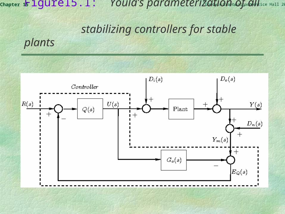
Figure15.1: Youla’s parameterization of all stabilizing controllers for stable plants

Chapter 15 Goodwin, Graebe, Salgado©
, Prentice Hall 2000
Modelling ErrorsThis description for the controller can also be used to give expressions for the achieved (or true) sensitivities when there exists model errors.Specifically, we have
where G (s) and G(s) are the additive and multiplicative modeling errors, respectively.

Chapter 15 Goodwin, Graebe, Salgado©
, Prentice Hall 2000
Nominal Design
Returning to the nominal design case (no modelling errors) we recall that
All of these equations are linear (strictly, affine) in Q(s). This makes design particularly straightforward.
Chapter 15 Goodwin, Graebe, Salgado©
, Prentice Hall 2000
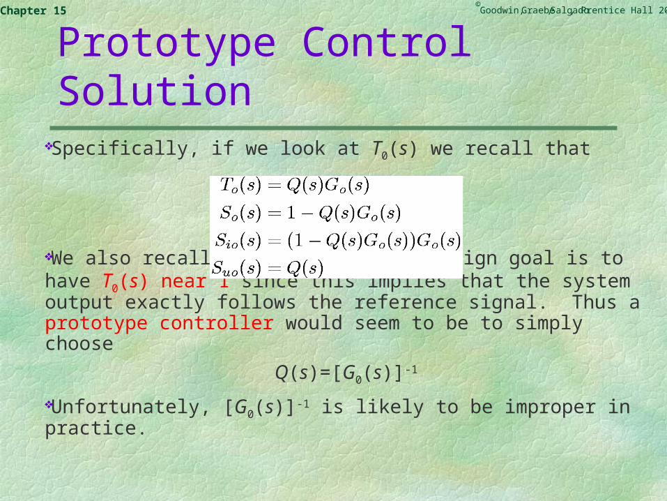
Prototype Control SolutionSpecifically, if we look at T0(s) we recall that
We also recall that a reasonable design goal is to have T0(s) near 1 since this implies that the system output exactly follows the reference signal. Thus a prototype controller would seem to be to simply choose
Q(s)=[G0(s)]-1
Unfortunately, [G0(s)]-1 is likely to be improper in practice.
Chapter 15 Goodwin, Graebe, Salgado©
, Prentice Hall 2000
Design Considerations
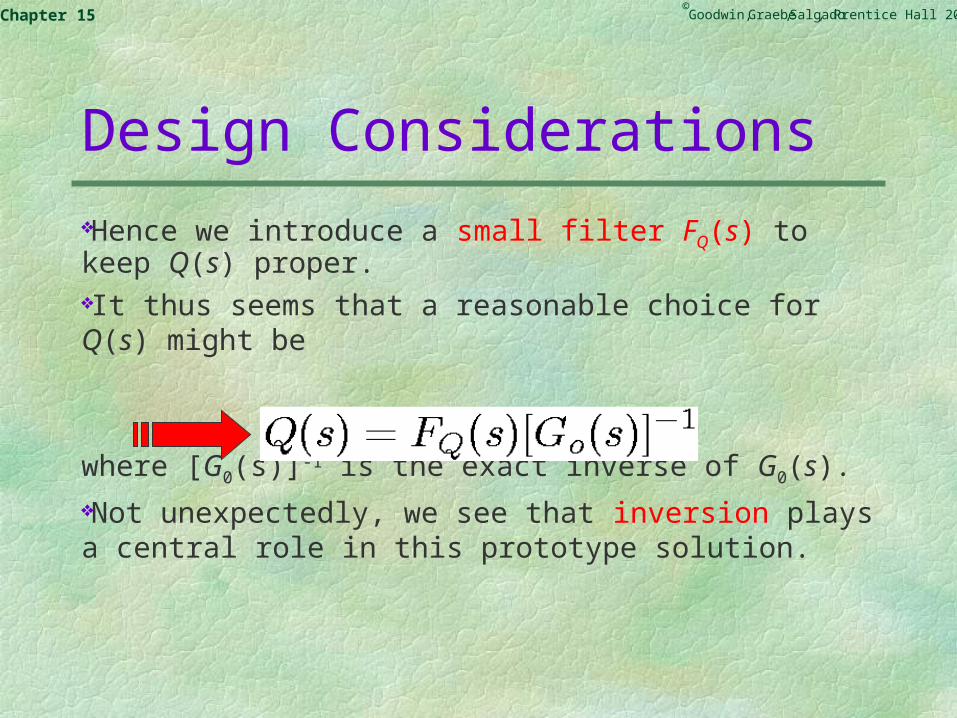
Hence we introduce a small filter FQ(s) to keep Q(s) proper.It thus seems that a reasonable choice for Q(s) might be
where [G0(s)]-1 is the exact inverse of G0(s).
Not unexpectedly, we see that inversion plays a central role in this prototype solution.
Chapter 15 Goodwin, Graebe, Salgado©
, Prentice Hall 2000
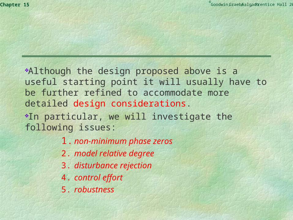
Although the design proposed above is a useful starting point it will usually have to be further refined to accommodate more detailed design considerations. In particular, we will investigate the following issues:
1. non-minimum phase zeros
2. model relative degree
3. disturbance rejection
4. control effort
5. robustness
Chapter 15 Goodwin, Graebe, Salgado©
, Prentice Hall 2000
1. Non Minimum Phase Zeros
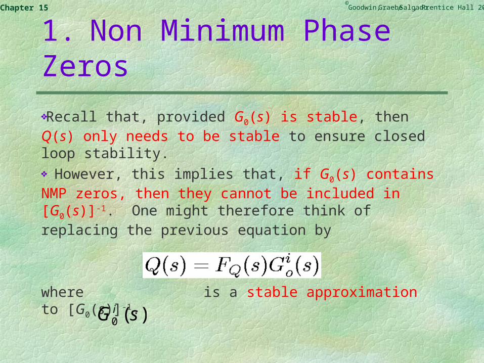
Recall that, provided G0(s) is stable, then Q(s) only needs to be stable to ensure closed loop stability. However, this implies that, if G0(s) contains NMP zeros, then they cannot be included in [G0(s)]-1. One might therefore think of replacing the previous equation by
where is a stable approximation to [G0(s)]-1.)(0 sG i
Chapter 15 Goodwin, Graebe, Salgado©
, Prentice Hall 2000
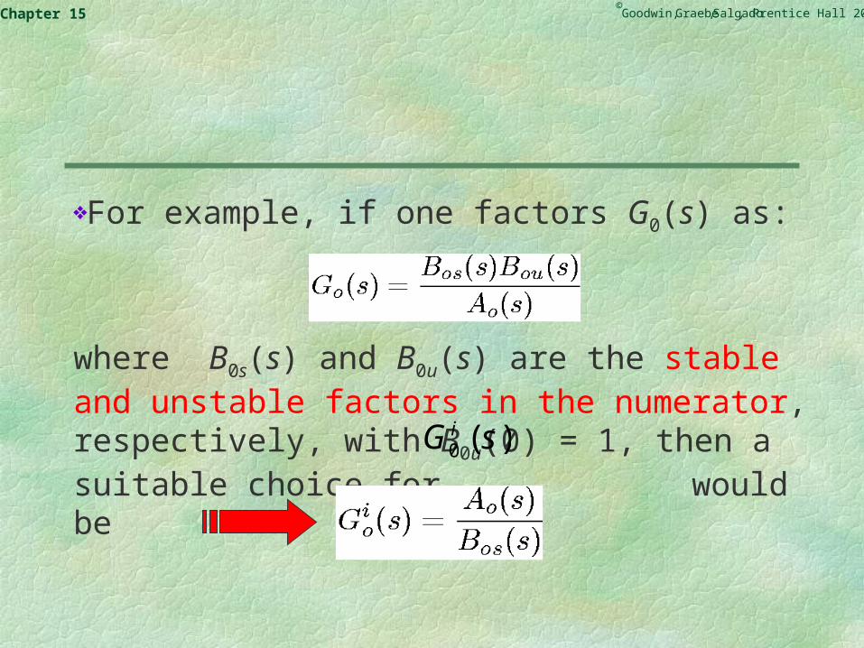
For example, if one factors G0(s) as:
where B0s(s) and B0u(s) are the stable and unstable factors in the numerator, respectively, with B0u(0) = 1, then a suitable choice for would be
)(0 sG i

Chapter 15 Goodwin, Graebe, Salgado©
, Prentice Hall 2000
2. Model Relative Degree
To have a proper controller it is necessary that Q(s) be proper. Thus it is necessary that the shaping filter, FQ(s) , have relative degree at least equal to the relative degree of nd.
Conceptually, this can be achieved by including factors of the form R in the denominator.
10 )]([ sG i
)()1( dns
Chapter 15 Goodwin, Graebe, Salgado©
, Prentice Hall 2000
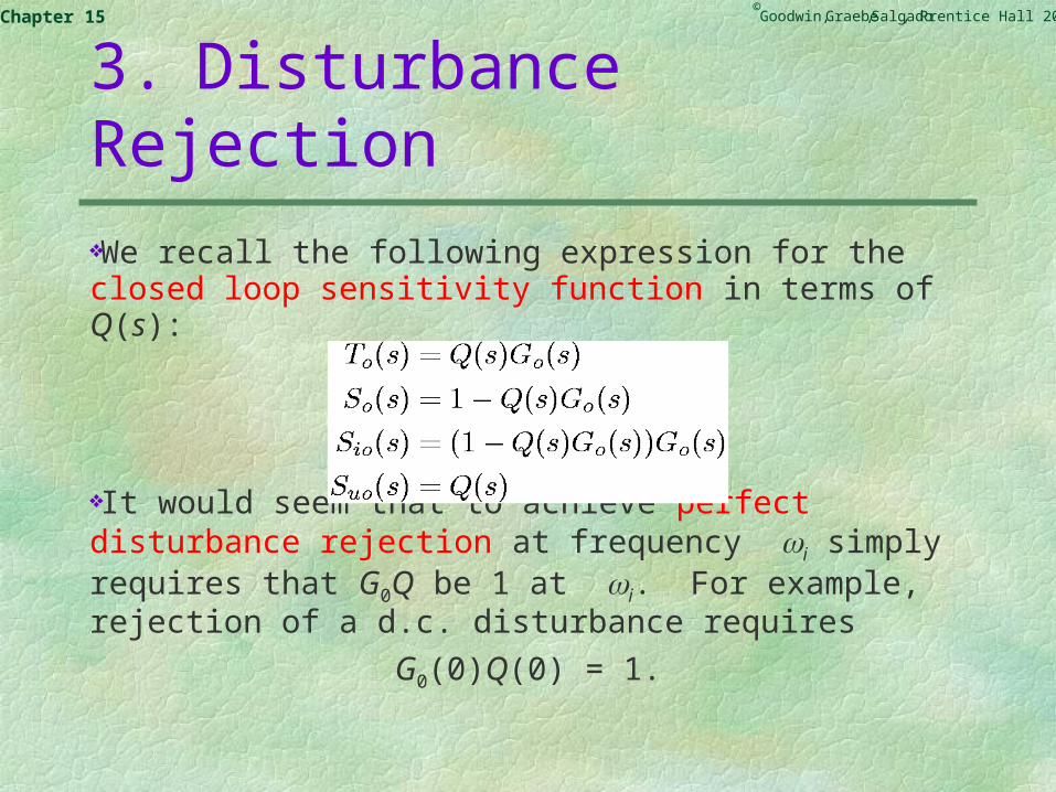
3. Disturbance Rejection
We recall the following expression for the closed loop sensitivity function in terms of Q(s):
It would seem that to achieve perfect disturbance rejection at frequency i simply requires that G0Q be 1 at i. For example, rejection of a d.c. disturbance requires
G0(0)Q(0) = 1.
Chapter 15 Goodwin, Graebe, Salgado©
, Prentice Hall 2000
All Stabilizing Controllers to give constant disturbance rejection
Once we have found one value of Q(s) (say we call it Qa(s)) that satisfies G0(0)Qa(0) = 1, then all possible controllers giving constant disturbance rejection can be described as shown on the next slide.

Chapter 15 Goodwin, Graebe, Salgado©
, Prentice Hall 2000
Consider a stable model G0(s) with input and/or output) disturbance at zero frequency. Then, a one d.o.f. control loop, giving zero steady state tracking error, is stable if and only if the controller C(s) can be expressed in the affine form where Q(s) satisfies
where is any stable transfer function, and Qa(s) is any stable transfer function which satisfies Qa(0) = 1.
)( sQ
Chapter 15 Goodwin, Graebe, Salgado©
, Prentice Hall 2000
Generalization
The above idea can be readily extended to cover rejection of disturbances at any frequency I.
Chapter 15 Goodwin, Graebe, Salgado©
, Prentice Hall 2000
4. Control Effort
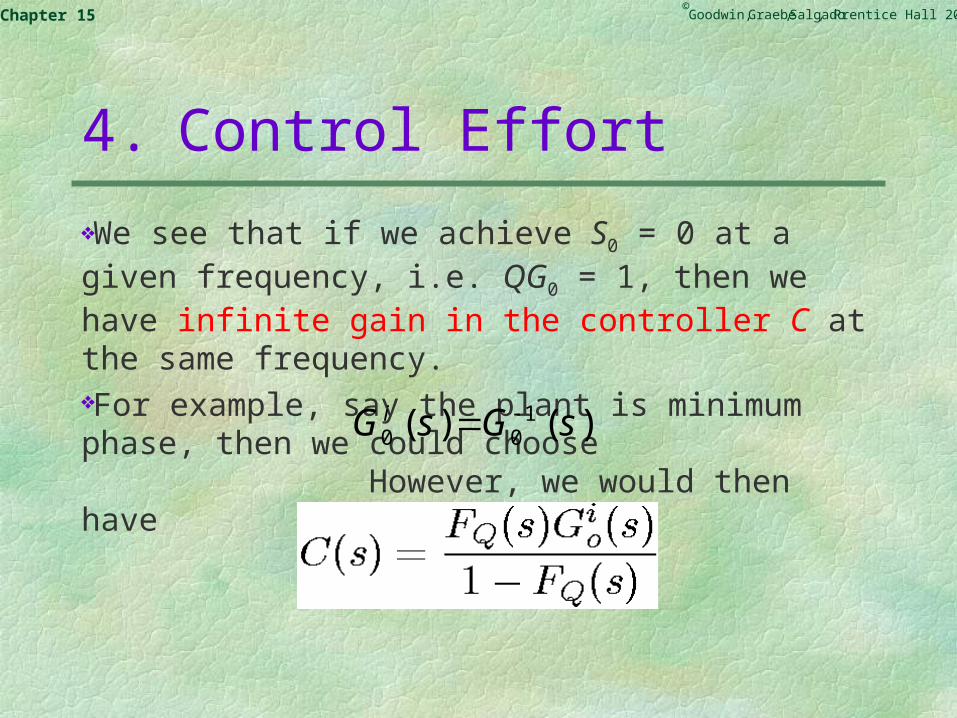
We see that if we achieve S0 = 0 at a given frequency, i.e. QG0 = 1, then we have infinite gain in the controller C at the same frequency. For example, say the plant is minimum phase, then we could choose However, we would then have
).()( 100 sGsG i
Chapter 15 Goodwin, Graebe, Salgado©
, Prentice Hall 2000
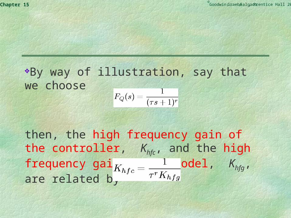
By way of illustration, say that we choose
then, the high frequency gain of the controller, Khfc, and the high frequency gain of the model, Khfg, are related by
Chapter 15 Goodwin, Graebe, Salgado©
, Prentice Hall 2000
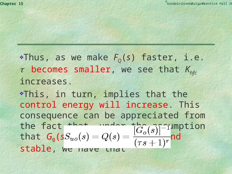
Thus, as we make FQ(s) faster, i.e. becomes smaller, we see that Khfc increases.
This, in turn, implies that the control energy will increase. This consequence can be appreciated from the fact that, under the assumption that G0(s) is minimum phase and stable, we have that
Chapter 15 Goodwin, Graebe, Salgado©
, Prentice Hall 2000
5. RobustnessFinally, we turn to the issue of robustness in choosing Q(s). We recall from earlier chapters that a fundamental result is that, in order to ensure robustness, the closed loop bandwidth should be such that the frequency response |T0(j)| rolls off before the effects of modelling errors become significant.Thus, in the framework of the affine parameterization under discussion here, the robustness requirement can be satisfied if FQ(s) reduces the gain of T0(j) at high frequencies.
This is usually achieved by including appropriate poles in FQ(s).
Chapter 15 Goodwin, Graebe, Salgado©
, Prentice Hall 2000
Choice of Q. Summary for the case of Stable Open Loop Poles
We have seen that a prototype choice for Q(s) is simply the inverse of the open loop plant transfer function G0(s). However, this ideal solution needs to be modified in practice to account for the following:
o Non-minimum phase zeros. Internal stability precludes the cancellation of these zeros. They must therefore appear in T0(s). This implies that the gain of Q(s) must be reduced at these frequencies for robustness reasons.
Chapter 15 Goodwin, Graebe, Salgado©
, Prentice Hall 2000
Relative degree. Excess poles in the model must necessarily appear as a lower bound for the relative degree of T0(s), since Q(s) must be proper to ensure that the controller C(s) is proper.
Disturbance trade-offs. Whenever we roll T0 off to satisfy measurement noise rejection, we necessarily increase sensitivity to output disturbances at that frequency. Also, slow open loop poles must either appear as poles of Si0(s) or as zeros of S0(s), and in either case there is a performance penalty.
Chapter 15 Goodwin, Graebe, Salgado©
, Prentice Hall 2000
Control energy. All plants are typically low pass. Hence, any attempt to make Q(s) close to the model inverse necessarily gives a high pass transfer function from D0(s) to U(s). This will lead to large input signals and may lead to controller saturation.
Robustness. Modeling errors usually become significant at high frequencies, and hence to retain robustness it is necessary to attenuate T0, and hence Q, at these frequencies.
Chapter 15 Goodwin, Graebe, Salgado©
, Prentice Hall 2000
PID Design Revisited
We have previously devoted Chapter 6 to Classical PID design. We will revisit this problem here using the affine parameterization. We will see that this makes certain aspects of the design very straightforward.
Chapter 15 Goodwin, Graebe, Salgado©
, Prentice Hall 2000
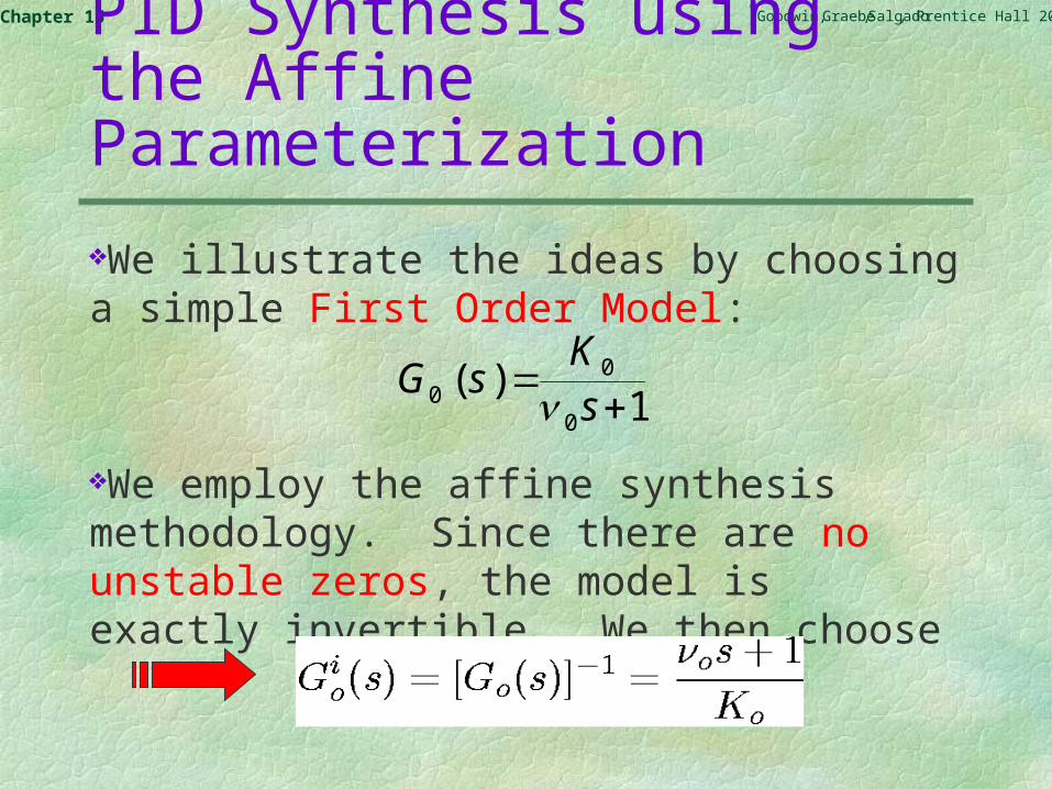
PID Synthesis using the Affine Parameterization
We illustrate the ideas by choosing a simple First Order Model:
We employ the affine synthesis methodology. Since there are no unstable zeros, the model is exactly invertible. We then choose
1)(
0
00
s
KsG
Chapter 15 Goodwin, Graebe, Salgado©
, Prentice Hall 2000
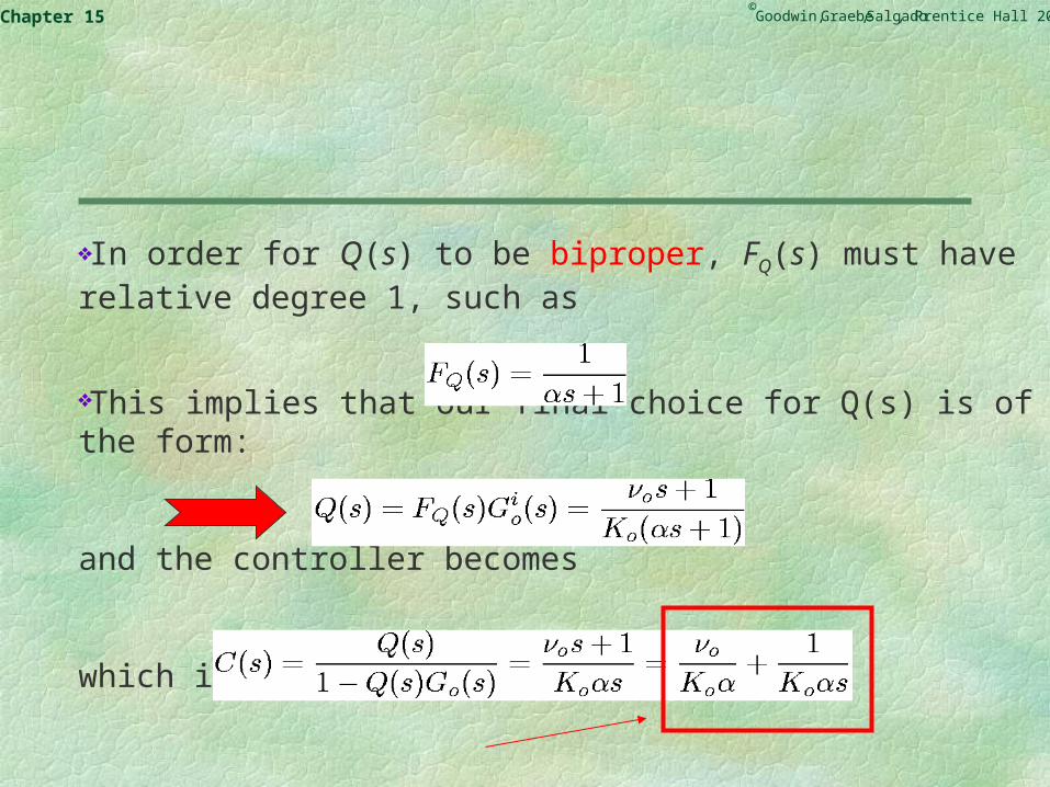
In order for Q(s) to be biproper, FQ(s) must have relative degree 1, such as
This implies that our final choice for Q(s) is of the form:
and the controller becomes
which is a PI controller.

Chapter 15 Goodwin, Graebe, Salgado©
, Prentice Hall 2000
Note that the above design is very straightforward.Properties of the design are discussed below.
Chapter 15 Goodwin, Graebe, Salgado©
, Prentice Hall 2000
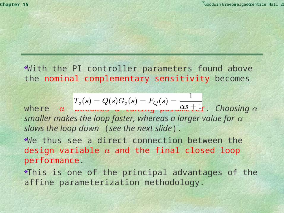
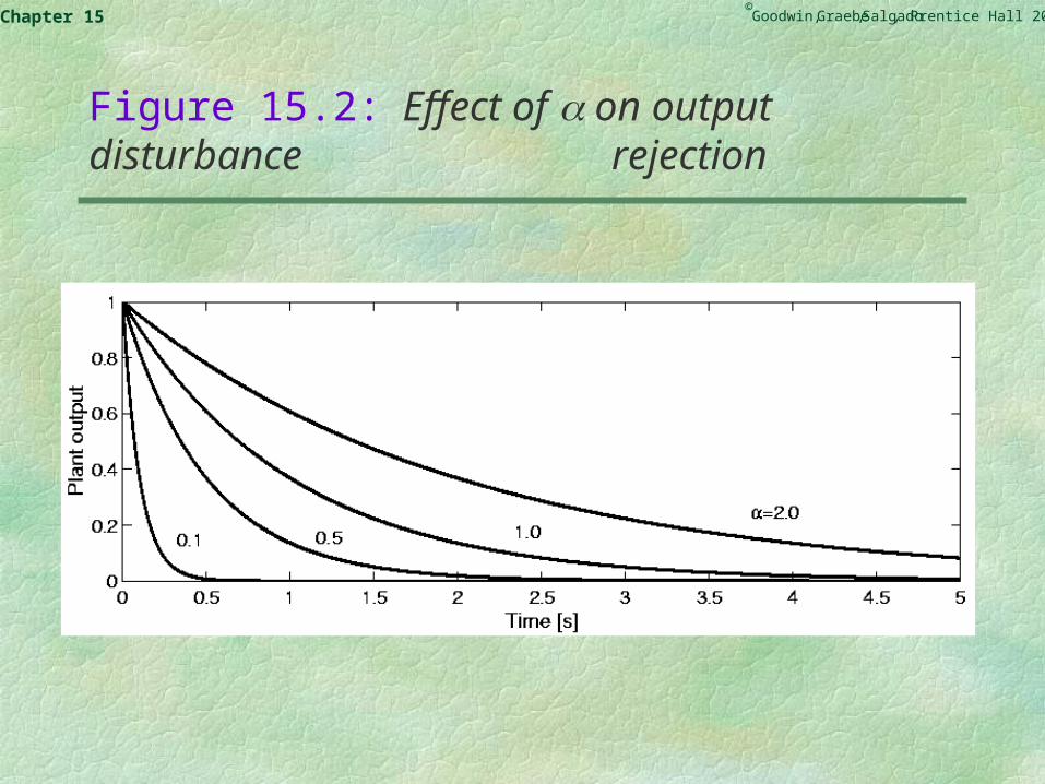
With the PI controller parameters found above the nominal complementary sensitivity becomes
where becomes a tuning parameter. Choosing smaller makes the loop faster, whereas a larger value for slows the loop down (see the next slide).We thus see a direct connection between the design variable and the final closed loop performance. This is one of the principal advantages of the affine parameterization methodology.
Chapter 15 Goodwin, Graebe, Salgado©
, Prentice Hall 2000
Figure 15.2: Effect of on output disturbance rejection
Chapter 15 Goodwin, Graebe, Salgado©
, Prentice Hall 2000
PID Design for Second Order Models
The book shows how the above ideas can be readily extended to second order models.
We will not go into details here. Instead, we consider a related topic - namely how to deal with pure time delays.
Chapter 15 Goodwin, Graebe, Salgado©
, Prentice Hall 2000
Affine Parameterization for Systems having Time Delays
We consider here a special class of linear systems, namely those that be written as
where is a stable rational transfer function.
A classical method for dealing with pure time delays as in the above model, was to use a dead-time compensator. This idea was introduced by Otto Smith in the 1950’s.
Here we give this a modern interpretation via the affine parameterization.
)(0 sG
Chapter 15 Goodwin, Graebe, Salgado©
, Prentice Hall 2000
Smith’s controller is based upon two key ideas: affine synthesis and the recognition that delay characteristics cannot be inverted. The structure of the traditional Smith controller can be obtained from the scheme in Figure 15.6, which is a particular case of the general scheme given earlier in Figure 15.1.
Chapter 15 Goodwin, Graebe, Salgado©
, Prentice Hall 2000
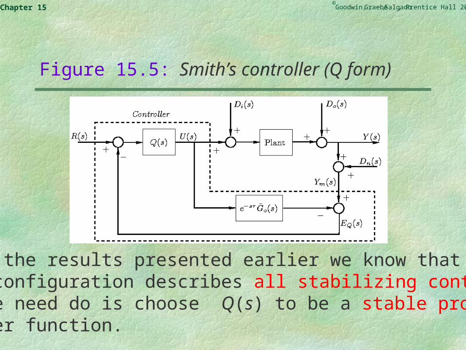
Figure 15.5: Smith’s controller (Q form)
•Using the results presented earlier we know that theabove configuration describes all stabilizing controllers.•All we need do is choose Q(s) to be a stable propertransfer function.
Chapter 15 Goodwin, Graebe, Salgado©
, Prentice Hall 2000
Design of Q(s) for Delayed Systems
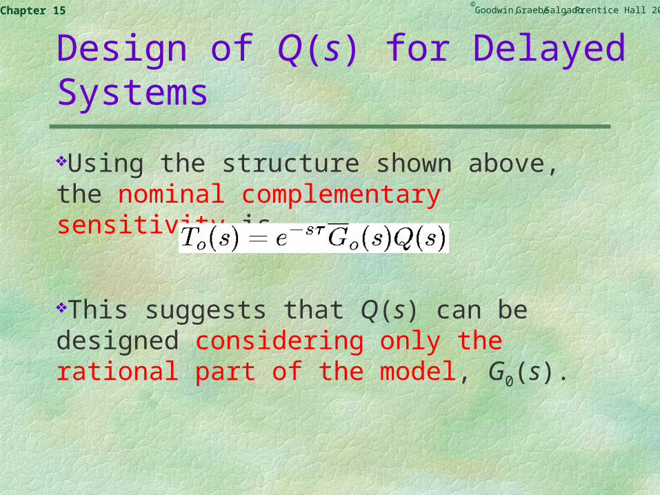
Using the structure shown above, the nominal complementary sensitivity is
This suggests that Q(s) can be designed considering only the rational part of the model, G0(s).
Chapter 15 Goodwin, Graebe, Salgado©
, Prentice Hall 2000
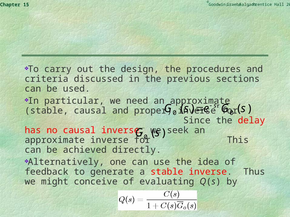
To carry out the design, the procedures and criteria discussed in the previous sections can be used. In particular, we need an approximate (stable, causal and proper) inverse for Since the delay has no causal inverse, we seek an approximate inverse for This can be achieved directly. Alternatively, one can use the idea of feedback to generate a stable inverse. Thus we might conceive of evaluating Q(s) by
).()( 00 sGesG s
).(0 sG
Chapter 15 Goodwin, Graebe, Salgado©
, Prentice Hall 2000
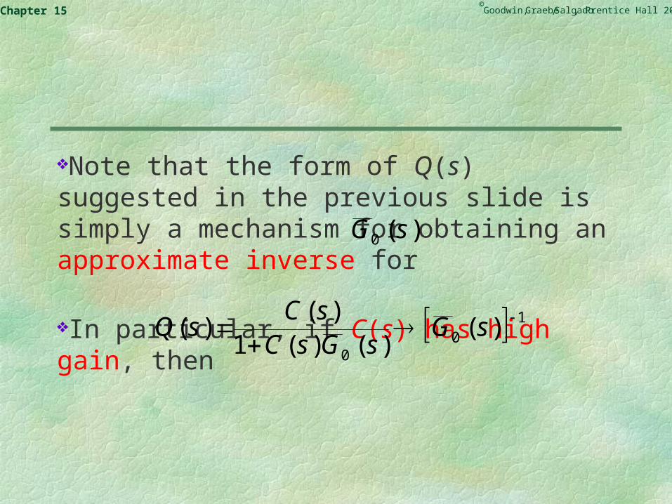
Note that the form of Q(s) suggested in the previous slide is simply a mechanism for obtaining an approximate inverse for In particular, if C(s) has high gain, then
).(0 sG
10
0
)()()(1
)()(
sG
sGsCsC
sQ
Chapter 15 Goodwin, Graebe, Salgado©
, Prentice Hall 2000
Redrawing the Controller
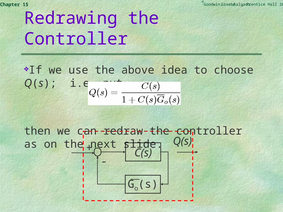
If we use the above idea to choose Q(s); i.e. put
then we can redraw the controller as on the next slide.
C(s)
Go(s)
+-
Q(s)
Chapter 15 Goodwin, Graebe, Salgado©
, Prentice Hall 2000
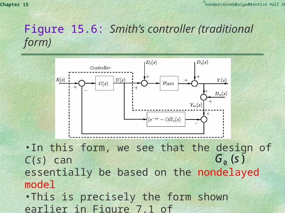
Figure 15.6: Smith’s controller (traditional form)
•In this form, we see that the design of C(s) canessentially be based on the nondelayed model •This is precisely the form shown earlier in Figure 7.1 ofSection 7.4 of Chapter 7. We ask the reader to reviewthe earlier design described in Chapter 7.
).(0 sG

Chapter 15 Goodwin, Graebe, Salgado©
, Prentice Hall 2000
Further Considerations
So far we have assumed that the nominal open loop plant model was stable. This meant that all we needed to do was to choose Q(s) to ensure closed loop stability. We next consider cases when G0(s) is not necessarily open loop stable.
Chapter 15 Goodwin, Graebe, Salgado©
, Prentice Hall 2000
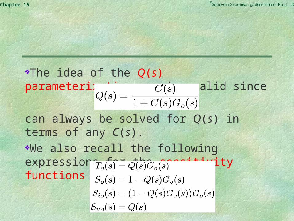
The idea of the Q(s) parameterization remains valid since
can always be solved for Q(s) in terms of any C(s).We also recall the following expressions for the sensitivity functions
Chapter 15 Goodwin, Graebe, Salgado©
, Prentice Hall 2000
In the case when G0(s) is not open loop stable, then we see that having Q(s) stable is a necessary condition for stability but is not sufficient.
Clearly to deal with open loop unstable models we will need to impose additional restrictions of Q(s).
This is the topic that we next consider.
Chapter 15 Goodwin, Graebe, Salgado©
, Prentice Hall 2000
Undesirable Closed Loop Poles
Up to this point is has been implicitly assumed that all open loop plant poles were stable and hence could be tolerated in the closed loop input sensitivity function Si0(s).
In practice we need to draw a distinction between stable poles and desirable poles. For example, a lightly damped resonant pair might well be stable but is probably undesirable. Say the open loop plant contains some undesirable (including unstable) poles. The only way to remove poles from the complementary sensitivity is to choose Q(s) to contain these poles as zeros.
Chapter 15 Goodwin, Graebe, Salgado©
, Prentice Hall 2000
This results in cancellation of these poles from the product Q(s)G0(s) and hence from S0(s) and T0(s).
However, the cancelled poles may still appear as poles of the nominal input sensivitity Si0(s), depending on the zeros of 1 - Q(s)G0(s), i.e. the zeros of S0(s).
To eliminate these poles from Si0(s) we need to also ensure that the offending poles are also zeros of [1 - Q(s)G0(s)].
The above represent a set of additional constraints on Q(s) to ensure closed loop stability. The result is summarized in the following lemma:
Chapter 15 Goodwin, Graebe, Salgado©
, Prentice Hall 2000
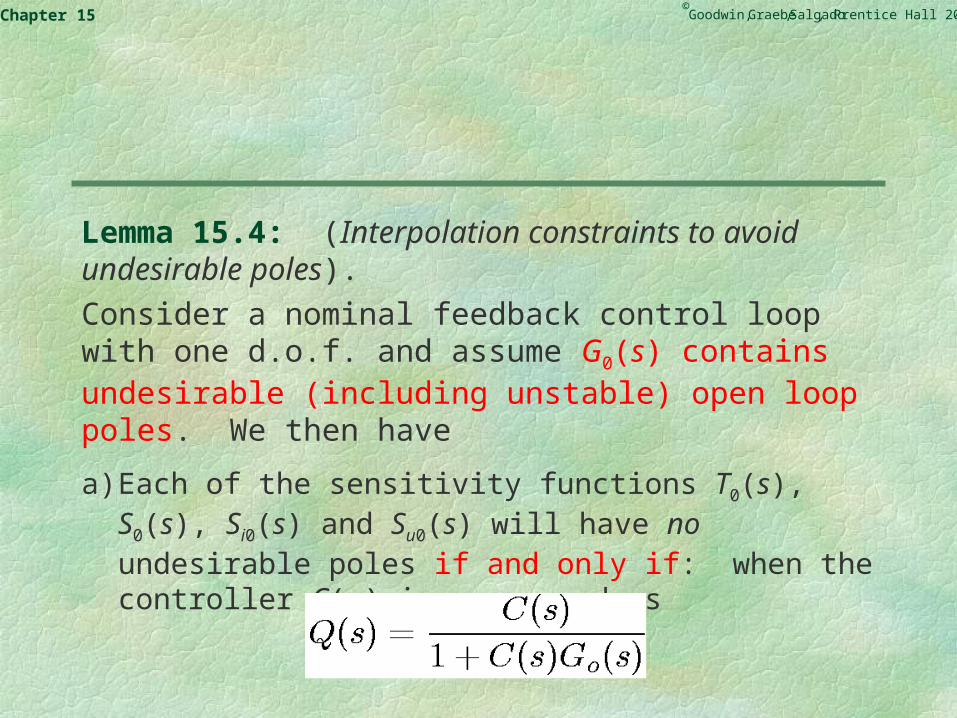
Lemma 15.4: (Interpolation constraints to avoid undesirable poles).
Consider a nominal feedback control loop with one d.o.f. and assume G0(s) contains undesirable (including unstable) open loop poles. We then have
a) Each of the sensitivity functions T0(s), S0(s), Si0(s) and Su0(s) will have no undesirable poles if and only if: when the controller C(s) is expressed as
Chapter 15 Goodwin, Graebe, Salgado©
, Prentice Hall 2000
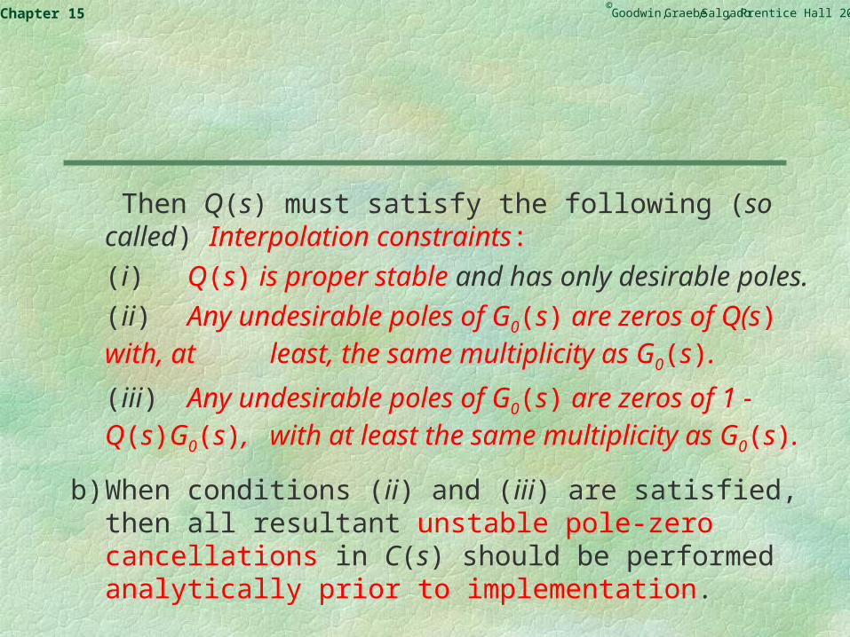
Then Q(s) must satisfy the following (so called) Interpolation constraints:
(i) Q(s) is proper stable and has only desirable poles.
(ii) Any undesirable poles of G0(s) are zeros of Q(s) with, at least, the same multiplicity as G0(s).
(iii) Any undesirable poles of G0(s) are zeros of 1 - Q(s)G0(s), with at least the same multiplicity as G0(s).
b) When conditions (ii) and (iii) are satisfied, then all resultant unstable pole-zero cancellations in C(s) should be performed analytically prior to implementation.
Chapter 15 Goodwin, Graebe, Salgado©
, Prentice Hall 2000
PID Design Revisited
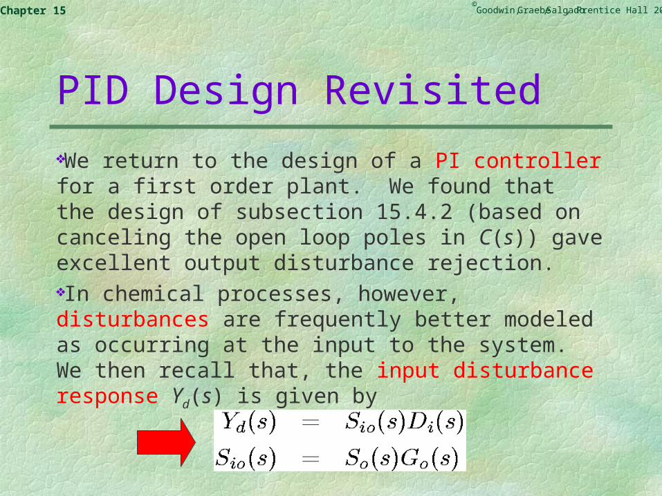
We return to the design of a PI controller for a first order plant. We found that the design of subsection 15.4.2 (based on canceling the open loop poles in C(s)) gave excellent output disturbance rejection. In chemical processes, however, disturbances are frequently better modeled as occurring at the input to the system. We then recall that, the input disturbance response Yd(s) is given by
Chapter 15 Goodwin, Graebe, Salgado©
, Prentice Hall 2000
Hence, when any plant pole is cancelled in the controller, it remains controllable from the input disturbance, and is still observable at the output. Thus the transient component in the input disturbance response will have a mode associated with that pole.
Chapter 15 Goodwin, Graebe, Salgado©
, Prentice Hall 2000
The following slide shows the input disturbance response for the PI controller designed earlier via the affine parameterization.
Chapter 15 Goodwin, Graebe, Salgado©
, Prentice Hall 2000
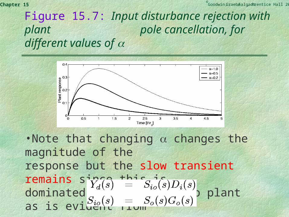
Figure 15.7: Input disturbance rejection with plant pole cancellation, for different values of
•Note that changing changes the magnitude of theresponse but the slow transient remains since this isdominated by the open loop plant as is evident from
Chapter 15 Goodwin, Graebe, Salgado©
, Prentice Hall 2000
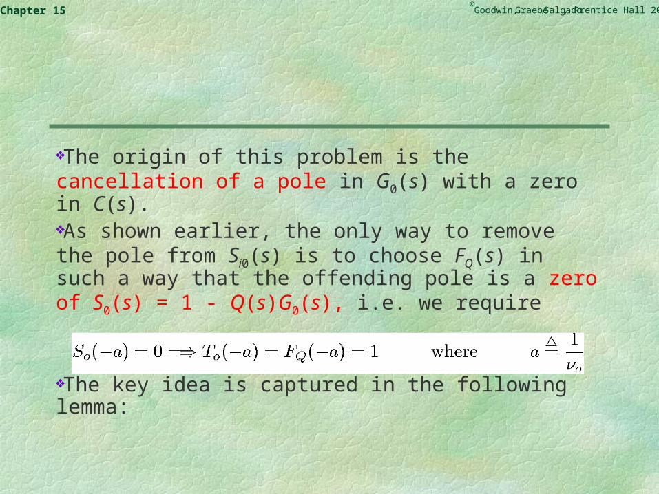
The origin of this problem is the cancellation of a pole in G0(s) with a zero in C(s). As shown earlier, the only way to remove the pole from Si0(s) is to choose FQ(s) in such a way that the offending pole is a zero of S0(s) = 1 - Q(s)G0(s), i.e. we require
The key idea is captured in the following lemma:
Chapter 15 Goodwin, Graebe, Salgado©
, Prentice Hall 2000
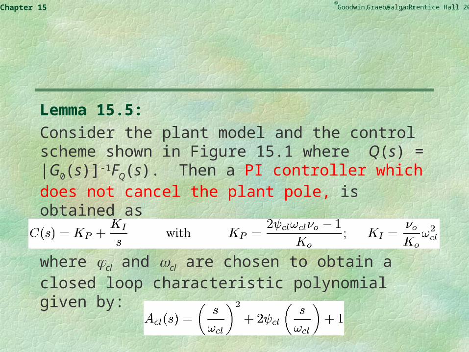
Lemma 15.5:
Consider the plant model and the control scheme shown in Figure 15.1 where Q(s) = |G0(s)]-1FQ(s). Then a PI controller which does not cancel the plant pole, is obtained as
where cl and cl are chosen to obtain a closed loop characteristic polynomial given by:
Chapter 15 Goodwin, Graebe, Salgado©
, Prentice Hall 2000
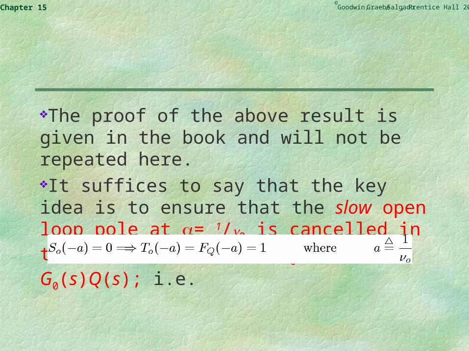
The proof of the above result is given in the book and will not be repeated here.It suffices to say that the key idea is to ensure that the slow open loop pole at = 1/0 is cancelled in the transfer function S0(s) = 1 - G0(s)Q(s); i.e.
Chapter 15 Goodwin, Graebe, Salgado©
, Prentice Hall 2000
We repeat the simulation presented earlier where = 1/0 remained in the input disturbance rejection response.
The new results are presented on the next slide.

Chapter 15 Goodwin, Graebe, Salgado©
, Prentice Hall 2000
Figure 15.8: Input disturbance rejection without plant pole cancellation

Chapter 15 Goodwin, Graebe, Salgado©
, Prentice Hall 2000
We see now that changing the design variable not only changes the size of the response but it also changes the nature of the transient.
(Compare Figure 15.8 with Figure 15.7).
Chapter 15 Goodwin, Graebe, Salgado©
, Prentice Hall 2000
Affine Parameterization: The Unstable Open Loop Case
In the examples given above we went to some trouble to ensure that the poles of all closed loop sensitivity functions (especially the input disturbance sensitivity, Si0) lay in desirable regions of the complex plane.
In this section, we will simplify this procedure by considering a general design problem in which the open loop plant can have one (or many) poles in undesirable regions.
Chapter 15 Goodwin, Graebe, Salgado©
, Prentice Hall 2000
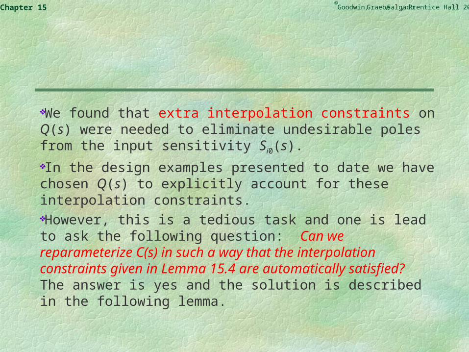
We found that extra interpolation constraints on Q(s) were needed to eliminate undesirable poles from the input sensitivity Si0(s).
In the design examples presented to date we have chosen Q(s) to explicitly account for these interpolation constraints. However, this is a tedious task and one is lead to ask the following question: Can we reparameterize C(s) in such a way that the interpolation constraints given in Lemma 15.4 are automatically satisfied? The answer is yes and the solution is described in the following lemma.
Chapter 15 Goodwin, Graebe, Salgado©
, Prentice Hall 2000
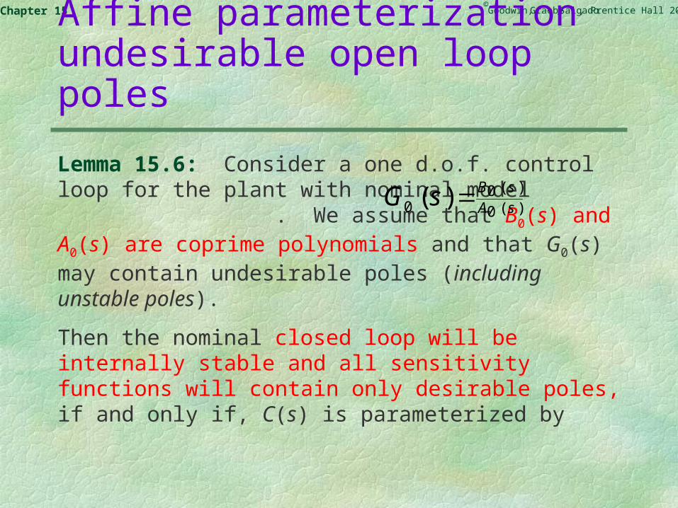
Affine parameterization undesirable open loop poles
Lemma 15.6: Consider a one d.o.f. control loop for the plant with nominal model . We assume that B0(s) and A0(s) are coprime polynomials and that G0(s) may contain undesirable poles (including unstable poles).
Then the nominal closed loop will be internally stable and all sensitivity functions will contain only desirable poles, if and only if, C(s) is parameterized by
)(0
)(00 )( sA
sBsG
Chapter 15 Goodwin, Graebe, Salgado©
, Prentice Hall 2000
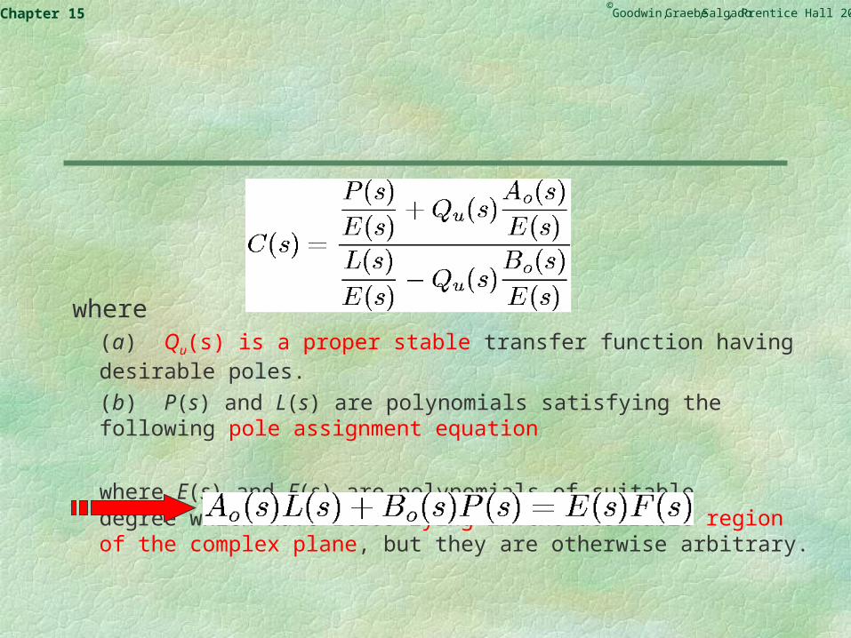
where(a) Qu(s) is a proper stable transfer function having desirable poles.
(b) P(s) and L(s) are polynomials satisfying the following pole assignment equation
where E(s) and F(s) are polynomials of suitable degree which have zeros lying in the desirable region of the complex plane, but they are otherwise arbitrary.
Chapter 15 Goodwin, Graebe, Salgado©
, Prentice Hall 2000
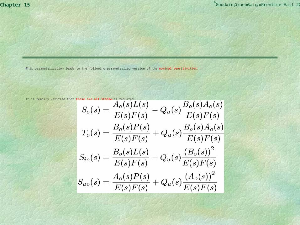
This parameterization leads to the following parameterized version of the nominal sensitivities:
It is readily verified that these are all stable as required.
Chapter 15 Goodwin, Graebe, Salgado©
, Prentice Hall 2000
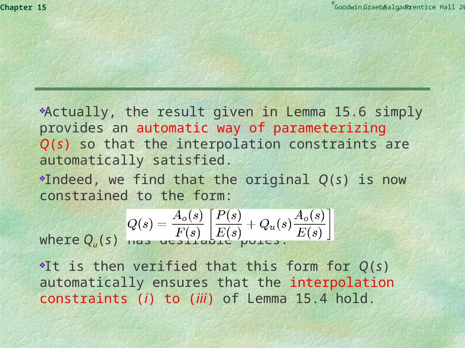
Actually, the result given in Lemma 15.6 simply provides an automatic way of parameterizing Q(s) so that the interpolation constraints are automatically satisfied. Indeed, we find that the original Q(s) is now constrained to the form:
where Qu(s) has desirable poles.
It is then verified that this form for Q(s) automatically ensures that the interpolation constraints (i) to (iii) of Lemma 15.4 hold.
Chapter 15 Goodwin, Graebe, Salgado©
, Prentice Hall 2000
The controller parameterization developed above can also be described in block diagram form. The equation for C(s) directly implies that the controller is as in Figure 15.9 (next slide).

Chapter 15 Goodwin, Graebe, Salgado©
, Prentice Hall 2000
Figure 15.9: Q parameterization for unstable plants
M(s)N(s)
Go(s)=N(s)/M(s)
Co(s)=U(s)/V(s)U(s)
V-1(s)
Chapter 15 Goodwin, Graebe, Salgado©
, Prentice Hall 2000
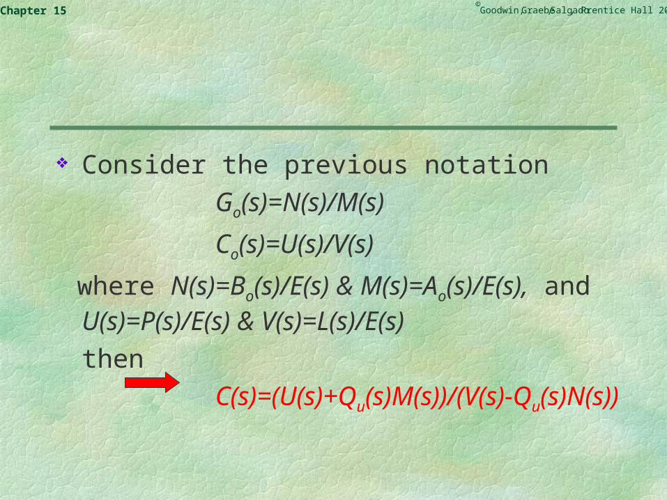
Consider the previous notation
Go(s)=N(s)/M(s)
Co(s)=U(s)/V(s)
where N(s)=Bo(s)/E(s) & M(s)=Ao(s)/E(s), and U(s)=P(s)/E(s) & V(s)=L(s)/E(s)
then
C(s)=(U(s)+Qu(s)M(s))/(V(s)-Qu(s)N(s))
Chapter 15 Goodwin, Graebe, Salgado©
, Prentice Hall 2000
The above parameterization of all stabilizing controllers for unstable systems, raises the following question:
“If we have an unstable open loop plant, why not simply apply pre-stabilizing feedback and then use the parameterization for the stable system so obtained?”
This is essentially the idea described in the above result as we next show. (It will turn out that there is a subtle difference).
Chapter 15 Goodwin, Graebe, Salgado©
, Prentice Hall 2000
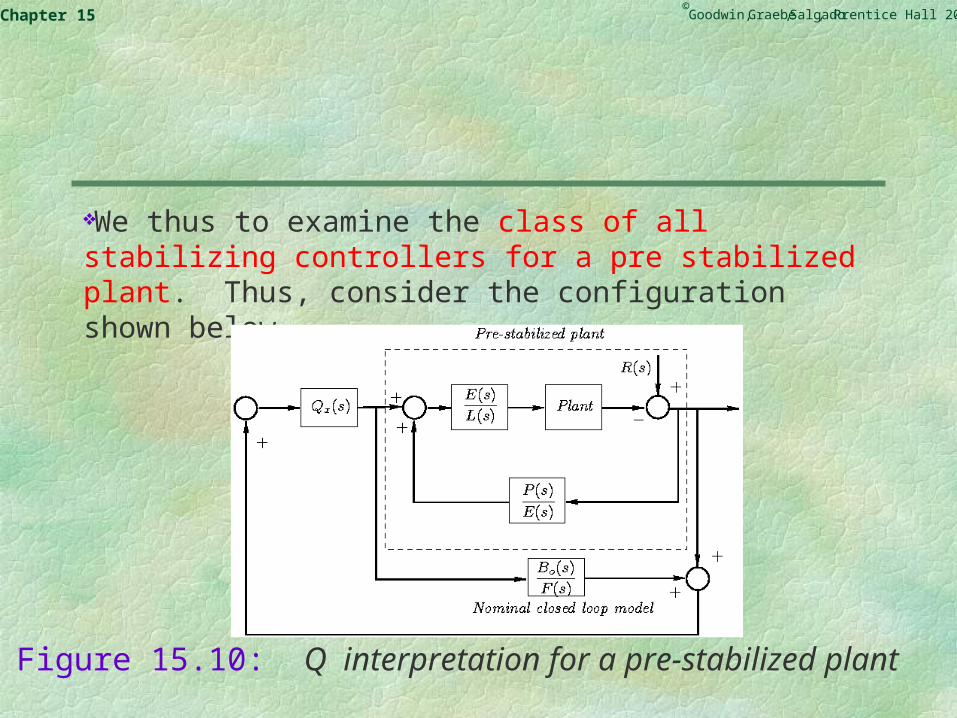
We thus to examine the class of all stabilizing controllers for a pre stabilized plant. Thus, consider the configuration shown below.
Figure 15.10: Q interpretation for a pre-stabilized plant
Chapter 15 Goodwin, Graebe, Salgado©
, Prentice Hall 2000
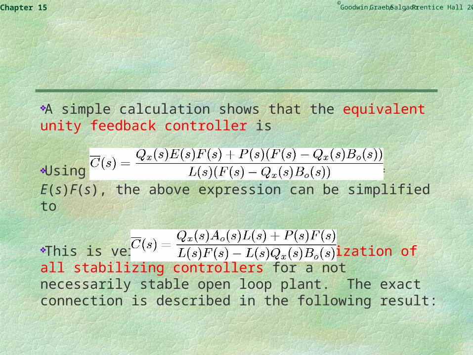
A simple calculation shows that the equivalent unity feedback controller is
Using the expression A0(s)L(s) + B0(s)P(s) = E(s)F(s), the above expression can be simplified to
This is very close to the parameterization of all stabilizing controllers for a not necessarily stable open loop plant. The exact connection is described in the following result:
Chapter 15 Goodwin, Graebe, Salgado©
, Prentice Hall 2000
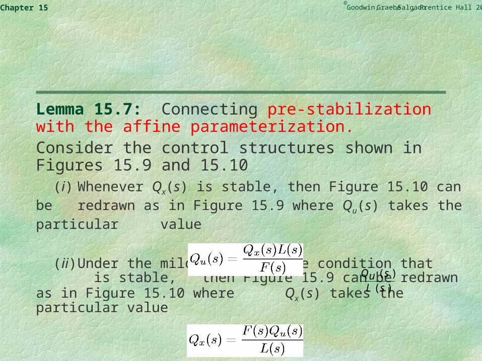
Lemma 15.7: Connecting pre-stabilization with the affine parameterization.Consider the control structures shown in Figures 15.9 and 15.10
(i) Whenever Qx(s) is stable, then Figure 15.10 can be redrawn as in Figure 15.9 where Qu(s) takes the particular value
(ii) Under the mildly restrictive condition that is stable, then Figure 15.9 can be redrawn as in Figure 15.10 where Qx(s) takes the particular value
)()(
sLsuQ
Chapter 15 Goodwin, Graebe, Salgado©
, Prentice Hall 2000
Part (i) of the above result is unsurprising, since the loop in Figure 15.10 is clearly stable for Qx(s) stable, and hence by Lemma 15.6 the controller can be expressed as in Figure 15.9 for some stable Qu(s).
The converse given in part (ii) is more interesting since it shows that there exist structures of the type shown in Figure 15.9 which cannot be expressed as in Figure 15.10.
Chapter 15 Goodwin, Graebe, Salgado©
, Prentice Hall 2000
Summary
The previous part of the book established that closed loop properties are interlocked in a network of trade offs. Hence, tuning for one property automatically impacts on other properties. This necessitates an understanding of the interrelations and conscious trade-off decisions.
The fundamental laws of trade-off presented in previous chapters allow one to both identify unachievable specifications as well as to establish where further effort is warranted or wasted.
Chapter 15 Goodwin, Graebe, Salgado©
, Prentice Hall 2000
However, when pushing a design maximally towards a subtle trade-off, the earlier formulation of the fundamental laws falls short because it is difficult to push the performance of a design by tuning in terms of controller numerator and denominator: The impact on the trade-off determining sensitivity-poles and zeros is very nonlinear, complex and subtle.
Chapter 15 Goodwin, Graebe, Salgado©
, Prentice Hall 2000
This shortcoming raises the need for an alternative controller representation that
allows one to design more explicitly in terms of the quantities of interest (the sensitivities),
makes stability explicit, and makes the impact of the controller on the trade-offs explicit.
This need is met by the affine parameterization, also known as Youla parameterization.
Chapter 15 Goodwin, Graebe, Salgado©
, Prentice Hall 2000
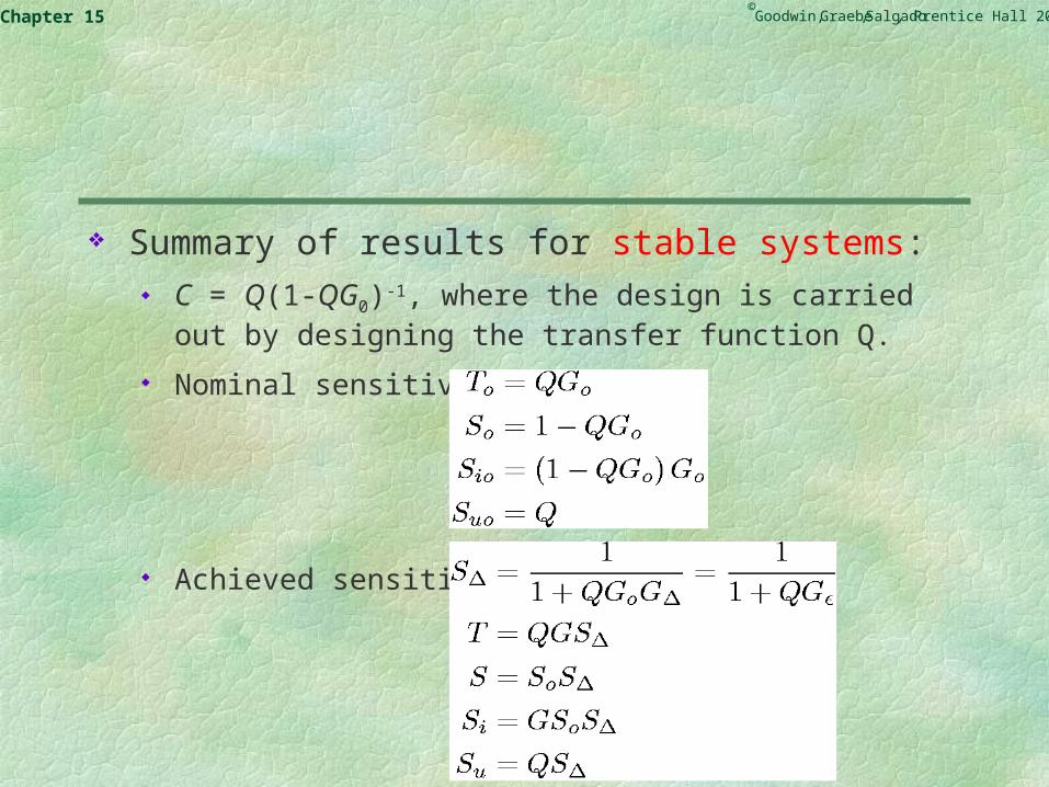
Summary of results for stable systems: C = Q(1-QG0)-1, where the design is carried out by designing the
transfer function Q.
Nominal sensitivities:
Achieved sensitivities:
Chapter 15 Goodwin, Graebe, Salgado©
, Prentice Hall 2000
Observe the following advantages of the affine parameterization: nominal stability is explicit
the known quantity G0 and the quantity sought by the control engineer (Q) occur in the highly insightful relation T0 = QG0 (multiplicative in the frequency domain); whether a designer chooses to work in this quantity from the beginning or prefers to start with a synthesis technique and then convert, the simple multiplicative relation QG0 provides deep insights into the trade-offs of a particular problem and provides a very direct means of pushing the design by shaping Q.
The sensitivities are affine in Q, which is a great advantage for synthesis techniques relying on numerical minimization of a criterion (see Chapter 16 for a detailed discussion of optimization methods which exploit this parameterization).
Chapter 15 Goodwin, Graebe, Salgado©
, Prentice Hall 2000
The following points are important to avoid some common misconceptions:
the associated trade-offs are not a consequence of the affine parameterization: they are perfectly general and hold for any linear time invariant controller including LQR, PID, pole placement based, H, etc.
we have used the affine parameterization to make the general trade-offs more visible and to provide a direct means for the control engineer to make trade-off decisions; this should not be confused with synthesis techniques that make particular choices in the affine parameterization to synthesize a controller.
The fact that Q must approximate the inverse of the model at frequencies where the sensitivity is meant to be small is perfectly general and highlights the fundamental importance of inversion in control. This does not necessarily mean that the controller, C, must contain this approximate inverse as a factor and should not be confused with the pros and cons of that particular design choice.

Chapter 15 Goodwin, Graebe, Salgado©
, Prentice Hall 2000
PI and PID design based on affine parameterization. PI and PID controllers are traditionally tuned in terms of their
parameters. However, systematic design, trade-off decisions and deciding whether
a PI(D) is sufficient or not, is significantly easier in the model-based affine structure.
Inserting a first order model into the affine structure automatically generates a PI controller.
Inserting a second order model into the Q-structure automatically generates a PID controller.
All trade-offs and insights of the previous chapters also apply to PID based control loops.
Chapter 15 Goodwin, Graebe, Salgado©
, Prentice Hall 2000
Whether a PI(D) is sufficient for a particular process is directly related to whether or not a first (second) order model can approximate the process well up to the frequencies where performance is limited by other factors such as delays, actuator saturations, sensor noise or fundamentally unknown dynamics.
The first and second order models are easily obtained from step response models (Chapter 3).
The chapter provides explicit formulas for first-order, time-delay second order and integrating processes.
Using this method, the control engineer works directly in terms of observable process properties (rise time, gain, etc.) and closed loop parameters providing an insightful basis for making trade-off decisions. The PI(D) parameters follow automatically.
Chapter 15 Goodwin, Graebe, Salgado©
, Prentice Hall 2000
Since the PI(D) parameter formulas are provided explicitly in terms of physical process parameters, the PI(D) gains can be scheduled to measurably changing parameters without extra effort (it is possible, for example, to schedule for a speed-dependent time-delay).
The approach does not preempt the design choice of canceling or shifting the open-loop poles - both are possible and associated with different trade-offs
Chapter 15 Goodwin, Graebe, Salgado©
, Prentice Hall 2000
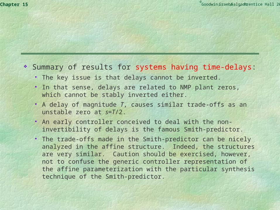
Summary of results for systems having time-delays: The key issue is that delays cannot be inverted. In that sense, delays are related to NMP plant zeros, which cannot be
stably inverted either. A delay of magnitude T, causes similar trade-offs as an unstable zero at
s=T/2. An early controller conceived to deal with the non-invertibility of delays
is the famous Smith-predictor. The trade-offs made in the Smith-predictor can be nicely analyzed in the
affine structure. Indeed, the structures are very similar. Caution should be exercised, however, not to confuse the generic controller representation of the affine parameterization with the particular synthesis technique of the Smith-predictor.
Chapter 15 Goodwin, Graebe, Salgado©
, Prentice Hall 2000
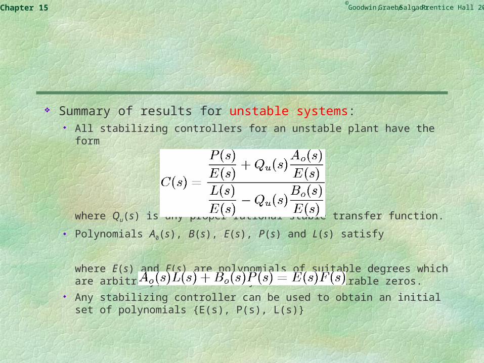
Summary of results for unstable systems: All stabilizing controllers for an unstable plant have the form
where Qu(s) is any proper rational stable transfer function.
Polynomials A0(s), B(s), E(s), P(s) and L(s) satisfy
where E(s) and F(s) are polynomials of suitable degrees which are arbitrary, save that they must have desirable zeros.
Any stabilizing controller can be used to obtain an initial set of polynomials {E(s), P(s), L(s)}


