61 CHAPTER 3 MODELING OF UPFC FOR ENHANCEMENT OF POWER SYSTEMS STABILITY 3.1 INTRODUCTION The control of AC power flow is a function of the transmission line impedance, the magnitude of the sending and receiving end voltages and the phase angle between these voltages. The idea behind Flexible AC Transmissions (FACTS) concept is to control these parameters in real time and there by vary (increase or decrease) almost instantaneously the transmitted power according to prevailing system conditions. The ability to control power rapidly within appropriately, defined boundaries can increase the transient (first swing) stability, as well as damping of the system. Increased transient stability and damping allow a corresponding increase in the transmittable steady-state power and thus a higher utilization of the system (Prabha Kundur 1994, Johns and Song 1999). Again due to steady increase in power demand, maintaining power system stability becomes a difficult and very challenging problem. The aim of this section of dissertation is to examine the ability of FACTS devices, such as Unified Power Flow Controller in damping of electromechanical oscillations in a power system. The UPFC is one of the most versatile flexible AC transmission system devices, which is a pair of back-to-back power electronic converters, can be used to control the active and reactive power flows in a transmission line by injecting a variable voltage in series and
Transcript
61
CHAPTER 3
MODELING OF UPFC FOR ENHANCEMENT OF POWER
SYSTEMS STABILITY
3.1 INTRODUCTION
The control of AC power flow is a function of the transmission line
impedance, the magnitude of the sending and receiving end voltages and the
phase angle between these voltages. The idea behind Flexible AC
Transmissions (FACTS) concept is to control these parameters in real time
and there by vary (increase or decrease) almost instantaneously the
transmitted power according to prevailing system conditions. The ability to
control power rapidly within appropriately, defined boundaries can increase
the transient (first swing) stability, as well as damping of the system.
Increased transient stability and damping allow a corresponding increase in
the transmittable steady-state power and thus a higher utilization of the
system (Prabha Kundur 1994, Johns and Song 1999).
Again due to steady increase in power demand, maintaining power
system stability becomes a difficult and very challenging problem. The aim
of this section of dissertation is to examine the ability of FACTS devices,
such as Unified Power Flow Controller in damping of electromechanical
oscillations in a power system. The UPFC is one of the most versatile
flexible AC transmission system devices, which is a pair of back-to-back
power electronic converters, can be used to control the active and reactive
power flows in a transmission line by injecting a variable voltage in series and
62
reactive current in shunt. A dynamic model of Unified Power Flow Controller
has been developed. This model can also be used to represent the system with
a Static Synchronous Compensator or a Static Synchronous Series
Compensator. The control strategy is based on d-q axis theory. In the present
work two different types of controllers are proposed for UPFC, namely
Genetic Algorithm (GA) tuned Proportional Integral (PI) and Single–Input
Fuzzy Logic Controller (SFLC). The above information is used in the Single
Machine Infinite Bus (SMIB) for carrying out transient stability studies.
3.1.1 Basic Circuit Configuration of UPFC
The advent of advanced power electronics technology has enabled
the use of voltage source inverters (VSI) at both the transmission and
distribution levels. A stream of VSI based systems such as UPFC,
STATCOM and SSSC has made the design of FACTS (Hingorani and
Gyugyi 2000) possible. Successful applications of FACTS equipment for
power flow control, voltage control and transient stability improvement have
been reported in the literature (Nabavi and Iravani 1996, Renz et al 1999,
Kannan et al 2004, Eskandar and Shahrokh 2005).
In recent years increasing interest has been seen in applying fuzzy
theory (Lee 1990) to controller design in many engineering fields. This
chapter focuses on the use of UPFC with SFLC (Byung-Jae Choi et al 2000)
for the Shunt and Series Inverter of the UPFC for transient stability
improvement and voltage control of power system. The principal function of
the UPFC is to control the flow of real and reactive power by injecting a
voltage in series with the transmission line. The UPFC consists of two solid-
state voltage source inverters connected by a common dc link that includes a
storage capacitor (shown in Figure 3.1).
63
Transmission Line uVcV
uV
SeriesTransformerSSSC
(Series Inverter)
ShuntTransformer
uV
uV
STATCOM(Shunt Inverter)
cV
dci dcV+-
CONTROLLER
DC link
Figure 3.1 Basic circuit configuration of the UPFC
The first inverter (shunt inverter) known as a STATCOM (Static
Synchronous Compensator) injects an almost sinusoidal current of variable
magnitude at the point of connection. The second inverter (series inverter),
known as SSSC (Static Synchronous Series Compensator) provides the main
functionality of the UPFC by injecting an AC voltage Vc, with a controllable
magnitude (0 Vc Vcmax) and phase angle ( 00, 3600). Thus, the
complete configuration operates as an ideal AC to AC power converter in
which real power can flow freely in either direction between the AC terminals
of the two inverters. The phasor diagram in Figure 3.1 illustrates that the
UPFC is able to inject a controlled series voltage Vc into the transmission
line. Thus, the magnitude and angle between the sending and receiving end of
the transmission line are modulated resulting in power flow control in the
transmission line. Therefore, the active power controller can significantly
affect the level of reactive power flow and vice versa. In order to improve the
dynamic performance and reduce the interaction between the active and
reactive power control, the watt-var decoupled control algorithm has been
64
proposed. In addition, each inverter can independently modulate reactive
power at its own AC output terminal.
The remainder of the chapter is organized as follows. At first, the
modeling of synchronous generator along with AVR and PSS, modeling of
UPFC and the conventional control scheme of a UPFC have been described
along with a study of the simulation results under transient disturbance.
Subsequently, the design of the proposed SFLC for the Shunt and Series
inverter of UPFC has been derived followed by a comparative evaluation of
this new controller’s performance via computer simulation results. Finally,
the conclusions of this study are reported.
3.2 MATHEMATICAL MODEL OF UPFC
Single machine infinite bus power system is considered in this
work. The load and the UPFC are connected at the load bus located between
the generator bus and the infinite-bus. The mathematical models for the
system components along with their control systems are described as follows:
3.2.1 Synchronous Generator Modeling
The synchronous generator is described by a third-order nonlinear
mathematical model given by equation (3.1 to 3.3).
dt (3.1)
qddqqqm iixxiEPM1
dt (3.2)
dddqfddo
q ixxEET1
dtEd
(3.3)
where 0 and 0 .
65
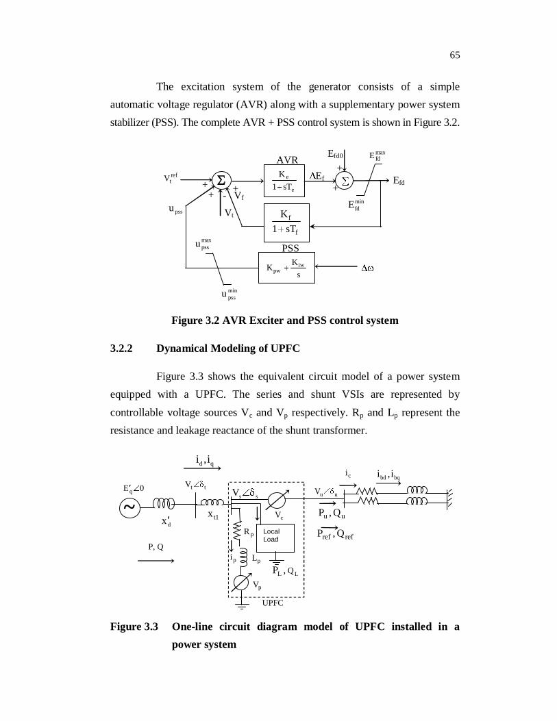
The excitation system of the generator consists of a simpleautomatic voltage regulator (AVR) along with a supplementary power systemstabilizer (PSS). The complete AVR + PSS control system is shown in Figure 3.2.
Efd0 maxfdE
sKK iw
pw
maxpssu
minpssu
e
e
sT1Kref
tV+
+ -Vtpssu
Ef+
+
minfdE
AVR
PSS
f
f
sT1K
+Vf
Efd
Figure 3.2 AVR Exciter and PSS control system
3.2.2 Dynamical Modeling of UPFC
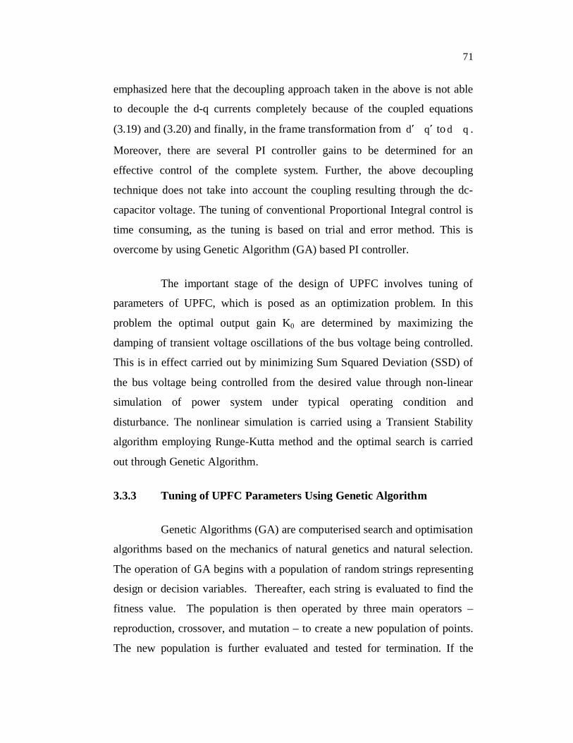
Figure 3.3 shows the equivalent circuit model of a power systemequipped with a UPFC. The series and shunt VSIs are represented bycontrollable voltage sources Vc and Vp respectively. Rp and Lp represent theresistance and leakage reactance of the shunt transformer.
qd i,i
0E q
bqbd i,i
~ttV
uuV
refref Q,P
ci
uu Q,P
pR
pL
pV
pi
cV
LocalLoad
ssV
1txdx
P, Q
LQ,PL
UPFC
Figure 3.3 One-line circuit diagram model of UPFC installed in apower system
66
The dynamic model of UPFC is derived by performing standard d-q
transformation of the current through the shunt transformer and series
transformer and is presented in equations (3.4 to 3.7).
Shunt Inverter
)V(VL1ii
LR
dtdi
pdsdp
pqpdp
ppd (3.4)
)V(VL1ii
LR
dtdi
pqsqp
pdpqp
ppq (3.5)
Series Inverter
)sinV(Vxw
iix
rwdt
dibud
e
bbqbd
e
ebbd (3.6)
)oscV(Vxw
iix
rwdt
dibuq
e
bbdbq
e
ebbq (3.7)
where is the angular frequency of the voltages and currents.
For fast voltage control, the net input power should instantaneously
meet the charging rate of the capacitor energy. Thus, by applying power
balance conditions, we get equation (3.8).
)iVi(V)i(iV)i(iVPP bquqbdudbqpqsqbdpdsdus
dcdc iV
dccpdc
dc Vgdt
dVCV (3.8)
Thus, equation 3.8 can be rearranged and written as given in equation (3.9).
bquqsqbdudsd
pqsqpdsd
dcdc
cp
cpdc
)iV(V)iV(V
iViV
CV1V
bg
dtdV (3.9)
67
3.3 CONVENTIONAL CONTROL STRATEGY FOR UPFC
Different controllers have been designed for the UPFC for reliable
and fast operation. As discussed earlier the UPFC has two VSIs connected
back to back. One can take the advantages to utilize any one of the VSI by
switching off the second one. The Shunt inverter injects an almost sinusoidal
current of magnitude, at the point of connection. There are two control
objectives in UPFC control, i.e., Shunt inverter control and Series inverter
control. For the Shunt inverter there are two voltage regulators designed for
this purpose: AC bus voltage regulators and DC voltage regulator. The real
and reactive power flow in the line can be controlled independently using the
series injected voltage which meets almost instantaneously to a command and
this voltage is generated by series inverter. The shunt inverter injects a
controlled shunt current (indirectly) by varying the shunt inverter voltage.
This inverter is responsible for AC-bus and DC-link voltage control
(indirectly). Therefore, in the PI control scheme, the control strategies for
both the inverters are addressed separately. The modeling and control design
are carried in the standard synchronous d-q frame.
3.3.1 Series Inverter Control
An appropriate series voltage (both magnitude and phase) should be
injected for obtaining the commanded active and reactive power flow in the
transmission line, i.e., uu Q,P . The current references are computed from the
desired power references and are given by equations (3.10 and 3.11),
2u
uqrefudrefrefcd
V
VQVPi (3.10)
2u
udrefuqrefrefcq
V
VQVPi (3.11)
68
The power flow control is then realized by using appropriately
designed controllers to force the line currents to track their respective
reference values. Conventionally, two separate PI controllers are used for this
purpose. These controllers output the amount of series injected
voltages )V,V( cqcd . The block diagram of series inverter control system is
shown in Figure 3.4.
Equations(3.10) and (3.11)
_
refcdi
+
refcqi
+cdi
refP
refQ
sKK id
pd
sK
K iqpq
cqV
cdV
_
icq
Figure 3.4 Series inverter control structure for UPFC
3.3.2 Shunt Inverter Control
As mentioned earlier, the conventional control strategy for this
inverter concerns with the control of ac-bus and dc-link voltage. The dual
control objectives are met by generating appropriate current reference (for
d and q axis) and then, by regulating those currents. PI controllers are
conventionally employed for both the tasks while attempting to decouple the
d and q axis current regulators.
q’q
s
d’
Vs
d
Figure 3.5 Phasor diagram showing d-q and d -q frame
69
In this study the strategy adopted in Padiyar and Kulkarni (1998)
for shunt current control has been taken. The inverter current ( pi ) is split into
real (in phase with ac-bus voltage) and reactive components. The reference
value for the real current is decided so that the capacitor voltage is regulated
by power balance. The reference for reactive component is determined by ac-
bus voltage regulator. As per the strategy, the original currents in d-q frame
)i,i( pqpd are now transformed into another frame, qd frame, where d
axis coincides with the ac-bus voltage )Vs( , as shown in Figure 3.5. Thus, in
qd frame, the currents dpi and qpi represent the real and reactive currents
and are given by equations (3.12 and 3.13).
spqspddpsinicosii (3.12)
spqspqqp sinicosii (3.13)
Now, for current control, the same procedure has been adopted by re
expressing the differential equations as given in equations (3.14 to 3.18).
)V(VL1ii
LR
dtdi
pd'sp
pq'pd'p
ppd' (3.14)
)V(L1i
LR
idt
di'pq
p'pq
p
p'pd
'pq (3.15)
where ssinVscosVV pqpdpd' (3.16)
ssinVcosVV pdspqpq' (3.17)
and dtd s
0 (3.18)
70
The VSI voltages are controlled as given in equations (3.19) and
(3.20).
)uLiL(V qp'pdp'pq (3.19)
dpspq'ppd' uLViLV (3.20)
By substituting the above expressions for dpV and qpV in equations (3.14) and
(3.15), the following sets of decoupled equations are obtained.
ddpp
pdp uiLR
dtdi
(3.21)
qqpp
pqp uiLR
dtdi
(3.22)
Conventionally, the control signals du and qu are determined by
linear PI controllers. The complete cascade control architecture is shown
below in Figure 3.6, where ,K,K,K,K,K,K,K dpqiqpicpcisps and diK are the
respective gains of the PI controllers.
Vpq
Vdc
Equation(3.19)
and(3.20)
VpdTransfor-mationfrom d’– q’ to d- q
Vpd’
Vpq’
uq
ud’
P I
Kps + Kis / s
Kpc + Kic / srefdcV
+
P I
P I
refsV
-
+
-
Kpq + Kiq / s
ref'pqi
ref'pdi
P Iipq’
+
-
ipd’
+
-
Kpd + Kid / s
Figure 3.6 Shunt inverter control structure for UPFC
In this study, the above design was used for demonstration of
UPFC control scheme. This approach leads to good control as illustrated by
the simulation results shown in later section (3.5). However, it must be
71
emphasized here that the decoupling approach taken in the above is not able
to decouple the d-q currents completely because of the coupled equations
(3.19) and (3.20) and finally, in the frame transformation from qd to qd .
Moreover, there are several PI controller gains to be determined for an
effective control of the complete system. Further, the above decoupling
technique does not take into account the coupling resulting through the dc-
capacitor voltage. The tuning of conventional Proportional Integral control is
time consuming, as the tuning is based on trial and error method. This is
overcome by using Genetic Algorithm (GA) based PI controller.
The important stage of the design of UPFC involves tuning of
parameters of UPFC, which is posed as an optimization problem. In this
problem the optimal output gain K0 are determined by maximizing the
damping of transient voltage oscillations of the bus voltage being controlled.
This is in effect carried out by minimizing Sum Squared Deviation (SSD) of
the bus voltage being controlled from the desired value through non-linear
simulation of power system under typical operating condition and
disturbance. The nonlinear simulation is carried using a Transient Stability
algorithm employing Runge-Kutta method and the optimal search is carried
out through Genetic Algorithm.
3.3.3 Tuning of UPFC Parameters Using Genetic Algorithm
Genetic Algorithms (GA) are computerised search and optimisation
algorithms based on the mechanics of natural genetics and natural selection.
The operation of GA begins with a population of random strings representing
design or decision variables. Thereafter, each string is evaluated to find the
fitness value. The population is then operated by three main operators –
reproduction, crossover, and mutation – to create a new population of points.
The new population is further evaluated and tested for termination. If the
72
termination criterion is not met, the population is iteratively operated by the
above three operators and evaluated. This procedure is continued until the
termination criterion is met. One cycle of these operations and the subsequent
evaluation procedure is known as a generation in GA’s terminology
(Goldberg 1989). The optimization problem for a power system with UPFC
is stated as follows:
Determine the optimal value of K0 to minimize the Sum Squared
Deviation index (SSDI) defined as follows:
nt 2ss
k 1SSDI V(k) V (3.23)
Subject to the following constraint:
K0min < K0 < K0max
where nt - total number of samples up to the final time of simulation
V(k) - the bus voltage at sampling time t = k T
Vss - bus voltage at the ntth sampling interval
Comparing the fitness function of both the parents and off springs,
the best strings will go for the next generation. Uniform crossover technique
proposed is used in this work, by which the convergence speed is faster than
the one-point and two-point crossovers. In this work the genetic iterations are
stopped where the difference between the minimum fitness and maximum
fitness is 0.001 or where the genetic iterations reached the maximum.
Advantage of genetic-algorithm technique is that the parameter limits can be
varied during the optimization, making the technique computationally
efficient but the limitation is the computational time associated with this
technique. GA parameters used for obtaining optimal PI parameter setting is
mentioned in Table 3.1.
73
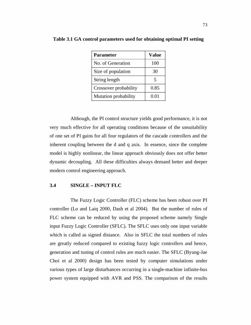
Table 3.1 GA control parameters used for obtaining optimal PI setting
Parameter ValueNo. of Generation 100
Size of population 30
String length 5
Crossover probability 0.85
Mutation probability 0.01
Although, the PI control structure yields good performance, it is not
very much effective for all operating conditions because of the unsuitability
of one set of PI gains for all four regulators of the cascade controllers and the
inherent coupling between the d and q axis. In essence, since the complete
model is highly nonlinear, the linear approach obviously does not offer better
dynamic decoupling. All these difficulties always demand better and deeper
modern control engineering approach.
3.4 SINGLE – INPUT FLC
The Fuzzy Logic Controller (FLC) scheme has been robust over PI
controller (Lo and Laiq 2000, Dash et al 2004). But the number of rules of
FLC scheme can be reduced by using the proposed scheme namely Single
input Fuzzy Logic Controller (SFLC). The SFLC uses only one input variable
which is called as signed distance. Also in SFLC the total numbers of rules
are greatly reduced compared to existing fuzzy logic controllers and hence,
generation and tuning of control rules are much easier. The SFLC (Byung-Jae
Choi et al 2000) design has been tested by computer simulations under
various types of large disturbances occurring in a single-machine infinite-bus
power system equipped with AVR and PSS. The comparison of the results
74
with conventional GA tuned PI cascaded control structure of UPFC reveals
the supremacy of the SFLC.
3.4.1 Design of SFLC
In existing fuzzy logic controllers (FLC), input variables are mostly
the error (e) and the change-of-error ( e ) regardless of complexity of
controlled plants. Either control input (u) or the change of control input ( u)
is commonly used as its output variable. A rule table is then constructed on a
two-dimensional (2-D) space. This scheme naturally inherits from
conventional proportional-derivative (PD) or proportional-integral (PI)
controller. Observing that 1) rule tables of most FLC’s have skew-symmetric
property and 2) the absolute magnitude of the control input |u| or | u| is
proportional to the distance from its main diagonal line in the normalized
input space, a new variable called the signed distance is derived, which is
used as a sole fuzzy input variable in our simple FLC called single-input FLC
(SFLC). The SFLC has many advantages: The total number of rules is greatly
reduced compared to existing FLC, and hence, generation and tuning of
control rules are much easier.
The rule form for the conventional (PI-type) FLC using two fuzzy
input variables of the error and the change-of-error is as follows:
If e is LEi and e is LDEi is then u is LUij where i = 1, 2,…M and
j = 1, 2, …..N, are the linguistic values taken by the process state variables e,
e and u respectively. Here the number of control rules is M x N. In case of
complex higher order plants, fuzzy input variables generally require all
process states. Then the number of rules is numerous and generation and
tuning of rules is very difficult. Hence, PD or PI-type FLC is used in many
applications regardless of the complexity of the controlled plants.
75
We first consider a control rule table of conventional FLC with the
control rule form, when every five linguistic values for error, change-of-error
and control input are used, a typical rule table is as shown in Table 3.2 with
25 rules.
Table 3.2 Rule base matrix for conventional FLC
e
eLE-2 LE-1 LE0 LE1 LE2
LDE2 LU0 LU-1 LU-1 LU-2 LU-2
LDE1 LU1 LU0 LU-1 LU-1 LU-2
LDE0 LU1 LU1 LU0 LU-1 LU-1
LDE-2 LU2 LU1 LU1 LU0 LU-1
LDE-1 LU2 LU2 LU1 LU1 LU0
In Table 3.2, subscripts –2, –1, 0, 1, and 2 denote fuzzy linguistic
values of negative big (NB), negative small (NS), zero (ZR), positive small
(PS) and positive big (PB), respectively. Similar to Table 3.2, most rule
tables have skew-symmetric property, namely, Uij = – Uij .
e
eZR
NR
NB
PSPB
e + e = 0
Figure 3.7 Rule table with infinitesimal quantization
76
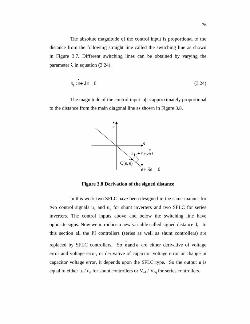
The absolute magnitude of the control input is proportional to the
distance from the following straight line called the switching line as shown
in Figure 3.7. Different switching lines can be obtained by varying the
parameter in equation (3.24).
: 0Sl e e (3.24)
The magnitude of the control input |u| is approximately proportional
to the distance from the main diagonal line as shown in Figure 3.8.
)e,P(e 11
)eQ(e,
1d
e
e
0ee
Figure 3.8 Derivation of the signed distance
In this work two SFLC have been designed in the same manner for
two control signals ud and uq for shunt inverters and two SFLC for series
inverters. The control inputs above and below the switching line have
opposite signs. Now we introduce a new variable called signed distance ds. In
this section all the PI controllers (series as well as shunt controllers) are
replaced by SFLC controllers. So eand e are either derivative of voltage
error and voltage error, or derivative of capacitor voltage error or change in
capacitor voltage error, it depends upon the SFLC type. So the output u is
equal to either ud / uq for shunt controllers or Vcd / Vcq for series controllers.
77
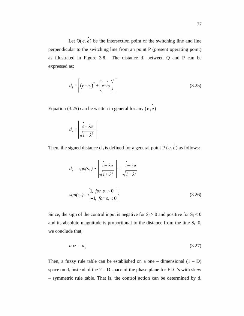
Let Q( e , e ) be the intersection point of the switching line and line
perpendicular to the switching line from an point P (present operating point)
as illustrated in Figure 3.8. The distance d1 between Q and P can be
expressed as:
2• •211 1d = e - e + e- e (3.25)
Equation (3.25) can be written in general for any ( e ,e )
•
s2
e+ ed =1+
Then, the signed distance d s is defined for a general point P (e ,e ) as follows:
•
s l2
e+ ed = sgn(s ) •1+
•
2
e+ e=1+
1, 01, 0
ll
l
for ssgn(s ) =
for s (3.26)
Since, the sign of the control input is negative for Sl > 0 and positive for Sl < 0
and its absolute magnitude is proportional to the distance from the line Sl=0,
we conclude that,
su d (3.27)
Then, a fuzzy rule table can be established on a one – dimensional (1 – D)
space on ds instead of the 2 – D space of the phase plane for FLC’s with skew
– symmetric rule table. That is, the control action can be determined by ds
78
only. So, we call it as SFLC. Figure 3.9 represents the fuzzy membership
functions sets for error, change-of-error, control input and signed distance.
The rule form for the SFLC is given as follows in Table 3.3. If ds is NB then
u is PB.
NB NS ZR PS PB
(x)
-1 0 1 x |---Wl---|
e, e , u and ds
Figure 3.9 The fuzzy membership functions
Table 3.3 Rule base matrix for SFLC
ds NB NS ZR PS PB
u PB PS ZR NS NB
where NB-big negative, NS-small negative, NR-Zero, PS-Small positive, PB-
positive big. Hence, the number of rules is greatly reduced compared to the
case of the conventional FLC. Furthermore, we can easily add or modify
rules for fine control. The defuzzification stage produces the final crisp
output of SFLC on the base of fuzzy input. The Root Sum Square (RSS)
method is employed for defuzzification.
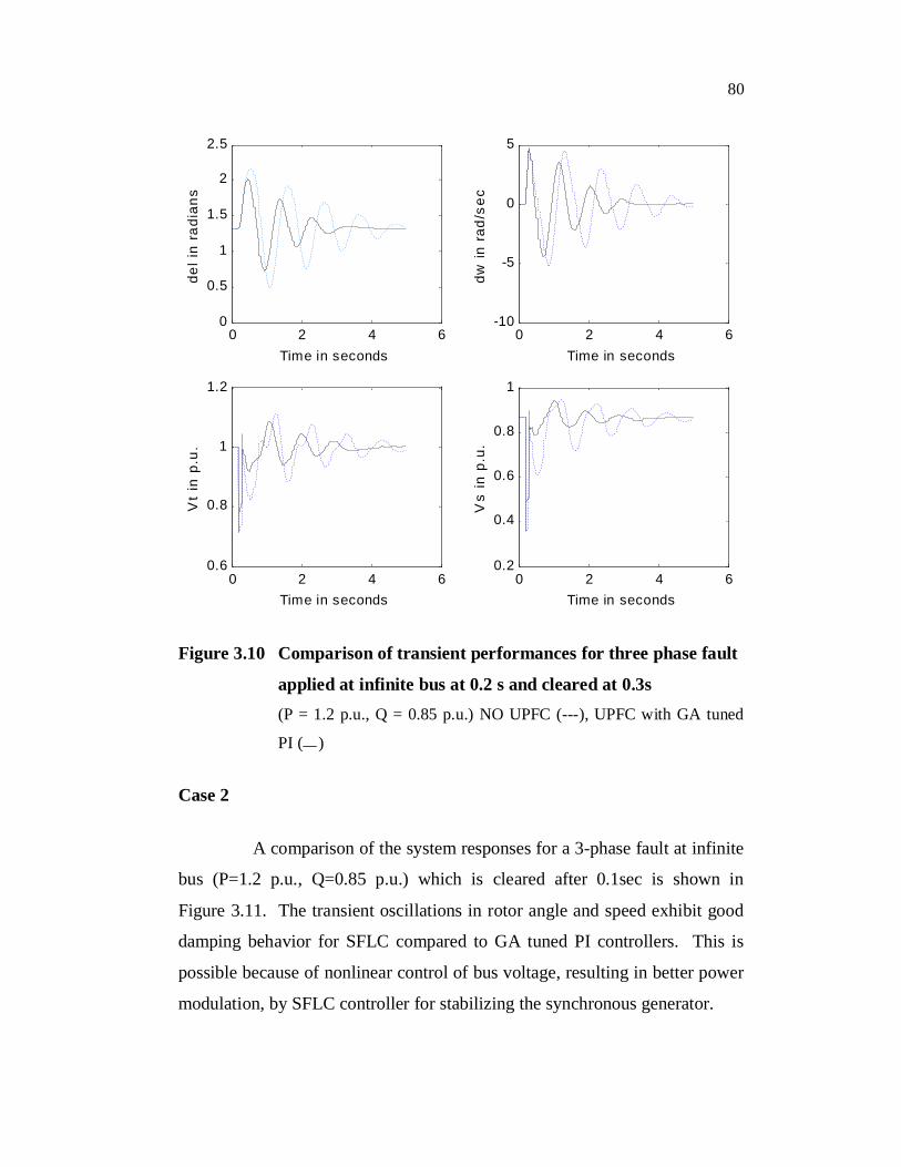
3.5 RESULTS AND DISCUSSION
The performance of the UPFC with GA tuned PI controller for
stabilization of synchronous generator is evaluated by computer simulation
studies. In the simulation studies UPFC has been connected to load bus of
79
SMIB. Then the result is compared with SFLC based UPFC for different