106 CHAPTER 5 ANALYSIS AND INTERPRETATION 5.1 INTRODUCTION - Peter Lewis This study has a set of goals for analysis and discussion. The first goal is to test the EI level of the 5 th year 9 th semester Medical students in Delhi. The second goal is to exhibit the profile of the respondents. The third goal is to assess the scores of each dimensions of the EI scale. The fourth goal is to assess the impact of age, gender and marital status on the level of EI among the medical students. The level of EI is assessed based on four dimensions: 1. Self-Emotion Appraisal 2. 3. Use of Emotion 4. Regulation of Emotion The validity of these dimensions is tested by examining whether they generate prototypes that are significantly different in those dimensions. The study concludes by sorting out the findings and suggestions derived from the analysis and interpretation. So it has been done through the various statistical tools, which were appropriately used for the study.
Transcript
106
CHAPTER 5
ANALYSIS AND INTERPRETATION
5.1 INTRODUCTION
- Peter Lewis
This study has a set of goals for analysis and discussion. The first goal
is to test the EI level of the 5th year 9th semester Medical students in Delhi.
The second goal is to exhibit the profile of the respondents. The third goal is
to assess the scores of each dimensions of the EI scale. The fourth goal is to
assess the impact of age, gender and marital status on the level of EI among
the medical students.
The level of EI is assessed based on four dimensions:
1. Self-Emotion Appraisal
2.
3. Use of Emotion
4. Regulation of Emotion
The validity of these dimensions is tested by examining whether they
generate prototypes that are significantly different in those dimensions.
The study concludes by sorting out the findings and suggestions
derived from the analysis and interpretation. So it has been done through the
various statistical tools, which were appropriately used for the study.
107
The data collected are tabulated and analyzed using the following
tools.
Descriptive Statistical Tools
Frequencies Procedure
Cross Tabulation
Inferential Statistical Tools
Chi-Square Test
ANOVA
T-Test
Correlation 5.1.1 Descriptive Statistics
5.1.1.1 Frequencies Procedure
The frequencies procedure is useful for obtaining summaries of
of the tasks that these summaries help us to complete are listed below.
iables. What values occur most
often? What range of values are we likely to see?
Checking the assumptions for statistical procedures. Do we have
enough observations? For each variable, is the observed distribution of
values adequate?
Checking the quality of the data. Are the missing or wrongly entered
values? Are the values that should be recorded?
108
5.1.1.2 Cross Tabulation
The cross tabulation technique is the basic technique for examining the
relationship between the two categorical (nominal or ordinal) variables,
possibly controlling for additional layering variables. The cross tabulation
procedure offers tests of independence and measures of association and
agreement for nominal and ordinal data. Additionally, estimates of the relative
risk of an event can be obtained given the presence or absence of a particular
characteristic. The cross tabulation shows the frequency of each response at
each store location. If each store location provides a similar level of service,
the pattern of responses should be similar across stores. At each store, the
majority of responses occur in the middle, from the cross tabulation alone, it
is impossible to tell whether these differences are real or due to chance
variation. The chi-square test has to be done to ensure this.
5.1.2 Inferential Statistics
5.1.2.1 Chi-Square Test
The chi-square test measures the discrepancy between the observed
cell counts and what would be expected if the rows and columns were
unrelated. The degree of influence of the following independent variables
pertaining to the respondents with respect to the factors influencing the level
of Emotional Intelligence are.
1. Age group of Respondents
2. Gender of Respondents
3. Marital status of Respondent
-e) 2 / E
With Degree of Freedom (D.F.) = (c-1) (r-1) where,
O= observed frequency
109
E= expected frequency
c= number of columns
r= number of rows
5.1.2.2 Anova Technique
The One-Way ANOVA procedure produces a one-way analysis of
variance for a quantitative dependent variable by a single factor variable.
Analysis of variance is used to test the hypothesis that several means are
equal. This technique is an extension of the two-sample t test. In addition to
determining that difference exists among the means, one may want to know
which means differ. There are two types of tests for comparing means: a
priori contrasts and post hoc tests. Contrasts are tests set up before running the
experiment and post hoc tests are run after the experiment has been
conducted. One can also test for trends across categories.
5.1.2.3 T-Test
A statistical examination of two population means. A two-sample t-test
examines whether two samples are different and is commonly used when the
variances of two normal distributions are unknown and when an experiment
uses a small sample size. 5.1.2.4 Correlation Correlation is the degree of association between variables in a set of
data. But, in a statistical sense, a correlation analysis usually produces a
measure of the linear relationship between the two variables. Therefore,
correlation analysis is closely related to regression analysis. Usually, there is a
misunderstanding about the relationship between correlation and causality.
Saying two variables are highly correlated does not necessarily mean that one
of the variables causes the other.
110
5.1.3 Reliability Analysis:
Reliability determines how consistently a measurement of skill or
knowledge yields similar results under varying conditions. If a measure has
high reliability, it yields consistent results. There are four principal ways to
estimate the reliability of a measure:
1. Inter-observer: Is determined by the extent to which different observers
or evaluators examine the same presentation, demonstration, project,
paper, or other performance and agree on the overall rating on one or
more dimensions.
2. Test-retest: Is determined by the extent to which the same test items or
kind of performance evaluated at two different times yields similar
results.
3. Parallel-forms: Is determined by examining the extent to which two
different measurements of knowledge or skill yield comparable results.
4. Split-half reliability: Is determined by comparing half of a set of test
items with the other half and determining the extent to which
they yield similar results.
The values for reliability coefficients range from 0.0 to 1.0. A coefficient
of 0 means no reliability and 1.0 mean perfect reliability. Since all tests have
some error, reliability coefficients never reach 1.0. Generally, if the reliably
of a standardized test above is 0.80, it is said to have very good reliability; if it
is below 0.50 it would not be considered a very reliable to test.
111
5.2 ANALYSIS
5.2.1 Reliability analysis
Table 5.1 Case Processing Summary
N %
Cases Valid 658 100.0
Excludeda 0 .0
Total 658 100.0
a. Least wise deletion based on all variables in the procedure. The above table 5.1 shows the number of valid responses, i.e., the total number of response is 658 (100%) and number of responses excluded is zero.
Table 5.2 Reliability Statistics
Cronbach's Alpha N of Items
.796 33
From the above table 5
(p = 0.796) which is significant that the researcher can continue with the
questionnaire for this study.
5.2.2 Structural Equation Modelling
Structural equation modelling (SEM) is a statistical technique for
testing and estimating causal relations using a combination of statistical data
and qualitative causal assumptions. This definition of SEM was articulated by
the geneticist Sewall Wright (1921), the economist Trygve Haavelmo (1943)
and the cognitive scientist Herbert A. Simon (1953), and formally defined by
Judea Pearl (2000) using a calculus of counterfactuals.
112
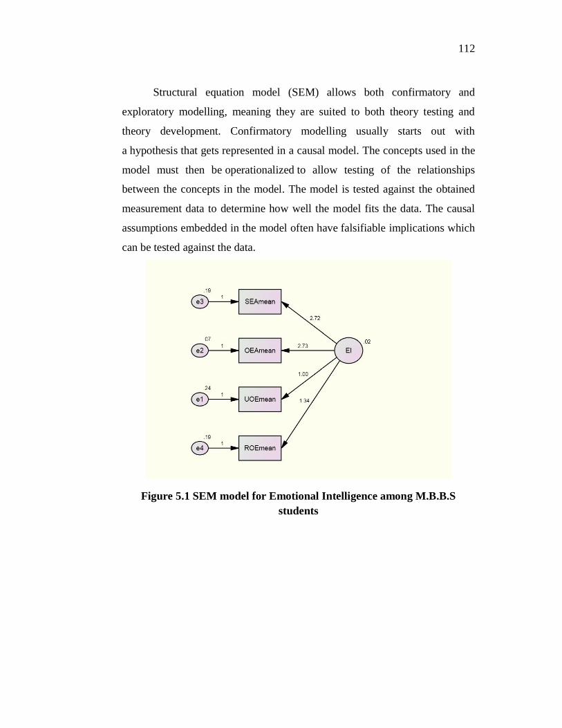
Structural equation model (SEM) allows both confirmatory and
exploratory modelling, meaning they are suited to both theory testing and
theory development. Confirmatory modelling usually starts out with
a hypothesis that gets represented in a causal model. The concepts used in the
model must then be operationalized to allow testing of the relationships
between the concepts in the model. The model is tested against the obtained
measurement data to determine how well the model fits the data. The causal
assumptions embedded in the model often have falsifiable implications which
can be tested against the data.
Figure 5.1 SEM model for Emotional Intelligence among M.B.B.S students
113
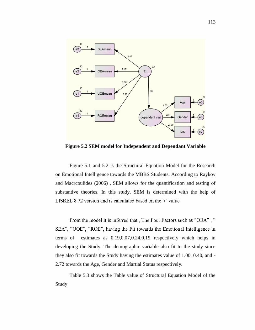
Figure 5.2 SEM model for Independent and Dependant Variable
Figure 5.1 and 5.2 is the Structural Equation Model for the Research
on Emotional Intelligence towards the MBBS Students. According to Raykov
and Macrcoulides (2006) , SEM allows for the quantification and testing of
substantive theories. In this study, SEM is determined with the help of
terms of estimates as 0.19,0.07,0.24,0.19 respectively which helps in
developing the Study. The demographic variable also fit to the study since
they also fit towards the Study having the estimates value of 1.00, 0.40, and -
2.72 towards the Age, Gender and Martial Status respectively.
Table 5.3 shows the Table value of Structural Equation Model of the
Study
114
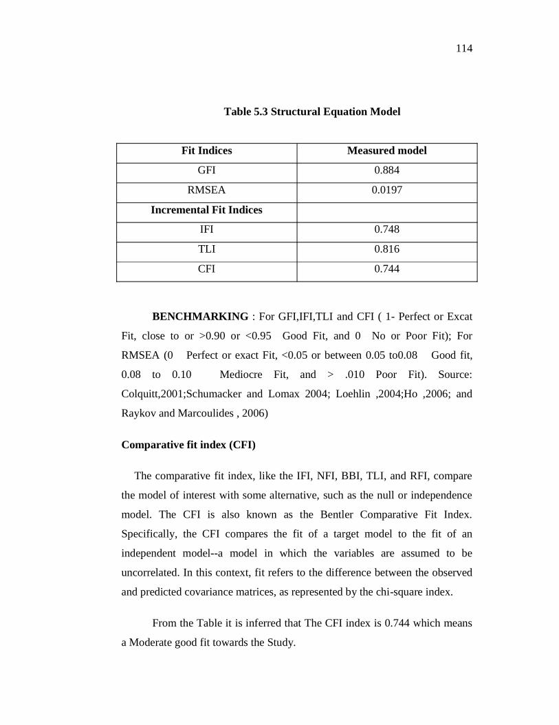
Table 5.3 Structural Equation Model
Fit Indices Measured model
GFI 0.884
RMSEA 0.0197
Incremental Fit Indices
IFI 0.748
TLI 0.816
CFI 0.744
BENCHMARKING : For GFI,IFI,TLI and CFI ( 1- Perfect or Excat
Fit, close to or >0.90 or <0.95 Good Fit, and 0 No or Poor Fit); For
RMSEA (0 Perfect or exact Fit, <0.05 or between 0.05 to0.08 Good fit,
0.08 to 0.10 Mediocre Fit, and > .010 Poor Fit). Source:
Colquitt,2001;Schumacker and Lomax 2004; Loehlin ,2004;Ho ,2006; and
Raykov and Marcoulides , 2006)
Comparative fit index (CFI)
The comparative fit index, like the IFI, NFI, BBI, TLI, and RFI, compare
the model of interest with some alternative, such as the null or independence
model. The CFI is also known as the Bentler Comparative Fit Index.
Specifically, the CFI compares the fit of a target model to the fit of an
independent model--a model in which the variables are assumed to be
uncorrelated. In this context, fit refers to the difference between the observed
and predicted covariance matrices, as represented by the chi-square index.
From the Table it is inferred that The CFI index is 0.744 which means
a Moderate good fit towards the Study.
115
Goodness of Fit Index (GFI)
The first measure of model fit is the Goodness-of-Fit Index (GFI). The
GFI measures the relative amount of variance and covariance in the Sample
covariance matrix that is jointly explained by the Population covariance
matrix. The GFI values range from 0 - 1, with values close to 1 being
indicative of good fit.
A second type of Goodness-of-Fit index used in the analysis can be classified
as incremental or comparative indexes of fit. As with the GFI, incremental
indexes of fit are based on a comparison of the hypothesized model against
some standard. However, whereas this standard represents no model at all for
the GFI, for the incremental indices, it represents a baseline model (typically
the independence or null model). Comparative Fit Index (CFI) is useful in that
it takes sample size into account. The CFI values range from 0 to 1, but
whereas .90 was considered a good fit for GFI.
From the table it is inferred that the Table value is 0.884, states that it is the
Good-fit towards the Thesis.
Incremental fit index (IFI)
The incremental fit index, also known as Bollen's IFI, is also relatively
insensitive to sample size. Values that exceed .90 are regarded as acceptable,
although this index can exceed 1.
To compute the IFI, first the difference between the chi square of the
independence model in which variables are uncorrelated--and the chi-square
of the target model is calculated. Next, the difference between the chi-square
of the target model and for the target model is calculated. The ratio of these
values represents the IFI.
116
From the Table Value it is found that, IFI =0.748, means that it is
Moderate good fit to acceptable one.
Root Mean Square Error of Approximation (RMSEA)
Mac Callum, Browne and Sugawara (1996) have used 0.01, 0.05, and 0.08
to indicate excellent, good, and mediocre fit, respectively. However, others
have suggested 0.10 as the cut off for poor fitting models. These are
definitions for the population. That is, a given model may have a population
value of 0.05 (which would not be known), but in the sample it might be
greater than 0.10. Use of confidence intervals and tests of PCLOSE can help
understand the sampling error in the RMSEA. There is greater sampling error
for small df and low N models, especially for the former. Thus, models with
small df and low N can have artificially large values of the RMSEA.
From the CFA Analysis, the RMSEA value is 0.0197 which means that
there is absolute measure of fit in the Research.
Tucker-Lewis index (TLI):
The Tucker-Lewis index, another incremental fit index, does have such a
penalty. TLI (Tucker-Lewis index, 1973), also known as NNFI (non-normed
fit index), similar to the next index presented, belongs to the class of
comparative fit indices, which are all based on a comparison of the implied
matrix with that of a null model (the most typical being that all observed
variables are uncorrelated). Those indices that do not be-long to this class,
such as RMSEA and SRMR, are called absolute fit indices
From the CFA Analysis, the TLI Value is 0.816 which means it is a good
fit towards the Research.
117
5.2.3 Normality Test:
Table 5.4 Normality Test
SEA OEA UOE ROE
N 658 658 658 658
Minimum 2 2 1 2
Maximum 5 5 5 5
Mean 3.83 3.77 3.40 3.64
Std. Deviation .584 0.486 0.506 0.475
Skewness Statistic -1.302 -0.628 -1.330 -0.758
Std. Error .095 0.095 0.095 0.095
Kurtosis Statistic 2.137 2.236 5.166 2.445
Std. Error .190 0.190 0.190 0.190
To check the normality of Data, Exploratory Data Analysis of each
Question was analysed separately. An Exploratory Data Analysis (EDA) for
the Factors in Emotional Intelligence having the each Factor is normally
distributed. From the Table 5.4, it is inferred that, SEA has the mean value
3.83 with standard deviation of 0.584, with the Skewness - -1.302 and
Kurtosis with 2.137. OEA has the mean value 3.77 with standard deviation of
0.486, with the Skewness - -0.628 and Kurtosis with 2.236, UOE having the
mean value 3.40 with standard deviation of 0.506, with the Skewness =-1.330
and Kurtosis with 0.190 and ROE mean 3.64 with standard deviation of
0.475, with the Skewness - -0.758 and Kurtosis with 0.190.The normality test
for SEA,OEA,UOE and ROE is given in Figures 5.3,5.4,5.5 and 5.6.
118
Figure 5.3 Normality Test for SEA
Figure 5.4 Normality Test for OEA
119
Figure 5.5 Normality Test for UOE
Figure 5.6 Normality Test for ROE
120
5.3. TO TEST THE LEVEL OF EMOTIONAL INTELLIGENCE OF
THE MBBS STUDENTS WITH THE HELP OF EMOTIONAL
INTELLIGENCE SCALE.
Table 5.5 Descriptive Statistics- Emotional Intelligence Mean score
N Minimum Maximum Mean Std. Deviation
Total Mean 658 2.62 4.47 3.5302 .32718 Valid N (list wise)
658
From the above table 5.5, it is inferred that the Mean value is 3.5302
towards the EI Level and it states its medium i.e., the level of EI is medium
among the 5th year 9th semester M.B.B.S. Students in Delhi. The EI level of
respondents is given in Figure 5.7.
Figure 5.7 EI level of Respondents
121
5.4 To Exhibit the profile of Respondents In social sciences research, personal characteristics of respondents
have very significant role to play in expressing and giving the responses about
the problem. Keeping this in mind, in this study a set of personal
characteristics namely, age, gender, and marital status of the 658 respondents
have been examined and presented in this chapter.
5.4.1 Age Wise Distribution of Respondent
Age of the respondents is one of the most important characteristics in
understanding their views about the particular problems. Higher age indicates
level of maturity of individuals in that sense age becomes more important to
examine the response.
Table 5.6 Details of Age of Respondents (Frequency Test)
Frequency Percent Valid Percent
Cumulative Percent
Valid 20 25 years 531 80.7 80.7 80.7
26 - 30 years 74 11.2 11.2 91.9
31 35 years 53 8.1 8.1 100.0
Total 658 100.0 100.0
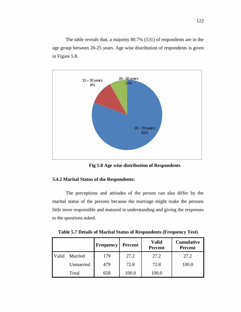
It is clear from the above table 5.6 that majority 80.7% (531) of
respondents are in the age group of 20-25 years, 11.2% (74) of respondents
are in the age group of 26-30 years and 8.1% (53) of respondents are in the
age group of 31-35 years.
122
The table reveals that, a majority 80.7% (531) of respondents are in the
age group between 20-25 years. Age wise distribution of respondents is given
in Figure 5.8.
Fig 5.8 Age wise distribution of Respondents
5.4.2 Marital Status of the Respondents:
The perceptions and attitudes of the person can also differ by the
marital status of the persons because the marriage might make the persons
little more responsible and matured in understanding and giving the responses
to the questions asked.
Table 5.7 Details of Marital Status of Respondents (Frequency Test)
Frequency Percent Valid Percent
Cumulative Percent
Valid Married 179 27.2 27.2 27.2
Unmarried 479 72.8 72.8 100.0
Total 658 100.0 100.0
20 25 years 81%
26 - 30 years 11%
31 35 years 8%
123
It is clear from the above table 5.7 that majority 72.8% (479) of
the respondents are unmarried whereas 27.2 % (179) of the respondents
are married.
The table reveals that, a majority 72.8% (479) are unmarried. The
marital status of respondents is given in Figure 5.9.
Fig 5.9 Marital status of respondents
5.4.3 Gender Wise Distribution of the Respondents
Gender is an important variable in a given Indian social situation
which is variably affected by any social or economic phenomenon and
globalization is not an exception to it. Hence the variable gender was
investigated for this study.
Married 27%
Unmarried 73%
124
Table 5.8 Details of Gender of Respondents (Frequency Test)
Frequency Percent Valid Percent Cumulative Percent
Valid Male 234 35.6 35.6 35.6
Female 424 64.4 64.4 100.0
Total 658 100.0 100.0
The above table 5.8 shows the Frequency table of Gender of the
Respondents. Majority 64.4% (424) of Respondents are female whereas
35.6% (234) respondents are Male. The Gender wise distribution of
Respondents is given in Figure 5.10.
Fig 5.10 Gender wise distribution of Respondents
5.5 ANALYSIS OF VARIANCE (ANOVA)
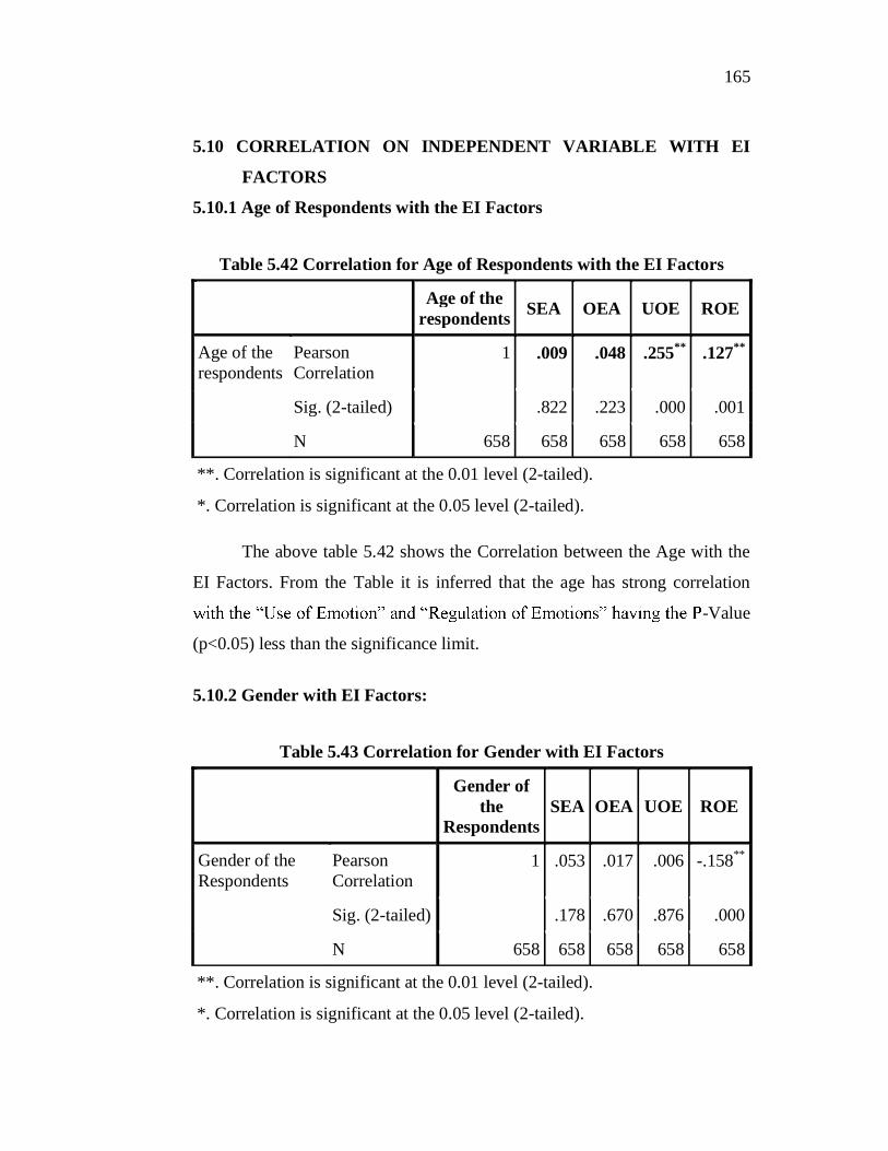
5.5.1 Age with EI Factors
Hypothesis:
Ho: There is no significant relationship between the Age with the EI factors
H1: There is significant relationship between the Age with EI Factors
Male 36%
Female 64%
125
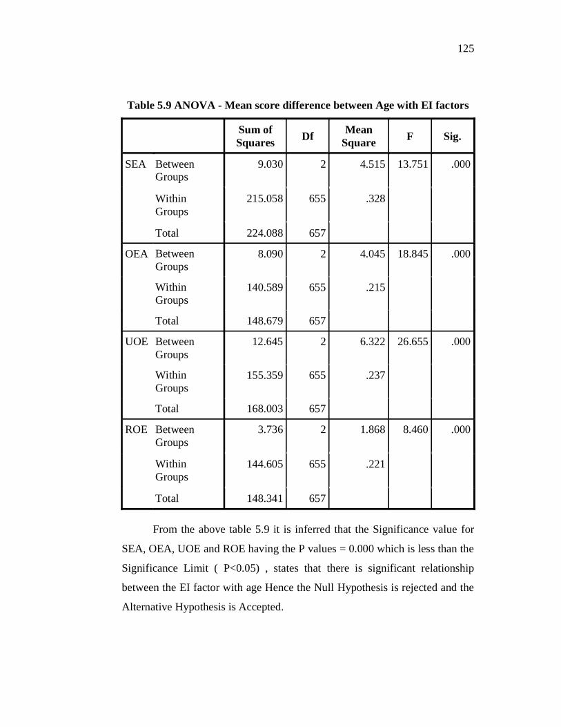
Table 5.9 ANOVA - Mean score difference between Age with EI factors
Sum of Squares Df Mean
Square F Sig.
SEA Between Groups
9.030 2 4.515 13.751 .000
Within Groups
215.058 655 .328
Total 224.088 657
OEA Between Groups
8.090 2 4.045 18.845 .000
Within Groups
140.589 655 .215
Total 148.679 657
UOE Between Groups
12.645 2 6.322 26.655 .000
Within Groups
155.359 655 .237
Total 168.003 657
ROE Between Groups
3.736 2 1.868 8.460 .000
Within Groups
144.605 655 .221
Total 148.341 657
From the above table 5.9 it is inferred that the Significance value for
SEA, OEA, UOE and ROE having the P values = 0.000 which is less than the
Significance Limit ( P<0.05) , states that there is significant relationship
between the EI factor with age Hence the Null Hypothesis is rejected and the
Alternative Hypothesis is Accepted.
126
5.5.2 Gender with EI Factors
Hypothesis:
Ho: There is no significant relationship between the Gender with the EI factors
H1: There is significant relationship between the Gender with EI Factors
Table 5.10 ANOVA
Mean score difference between Gender with EI factors
Sum of Squares Df Mean
Square F Sig.
SEA Between Groups
.618 1 .618 1.815 .178
Within Groups
223.469 656 .341
Total 224.088 657 OEA Between
Groups .041 1 .041 .181 .670
Within Groups
148.638 656 .227
Total 148.679 657 UOE Between
Groups .006 1 .006 .025 .876
Within Groups
167.997 656 .256
Total 168.003 657 ROE Between
Groups 3.700 1 3.700 16.783 .000
Within Groups
144.640 656 .220
Total 148.341 657
From the above table 5.10 it is inferred that the Significance value for
SEA, OEA, UOE having the P- values = 0.178, 0.670, 0.876 respectively
which is greater than the Significance Limit (P> 0.05) , states that there is no
significant relationship between the EI factor with Gender. Whereas the ROE
having the P-value less than the Significance Limit (P<0.05) states that there
is a significant relationship between ROE with Gender Factors.
127
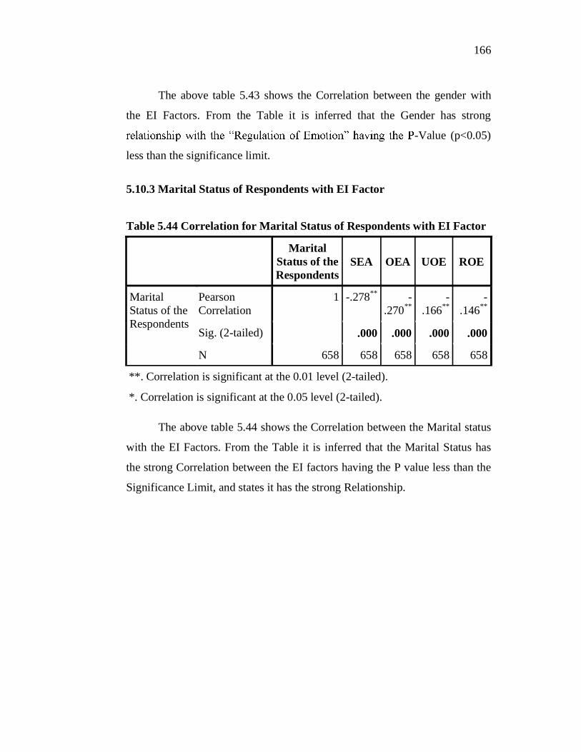
5.5.3 Marital Status with EI Factors
Hypothesis:
Ho: There is no significant relationship between the marital status with the EI
factors
H1: There is significant relationship between the marital status with EI
factors
Table 5.11 ANOVA
Mean score difference between Marital Status with EI factors
Sum of Squares Df Mean
Square F Sig.
SEA Between Groups
17.279 1 17.279 54.809 .000
Within Groups
206.809 656 .315
Total 224.088 657
OEA Between Groups
10.824 1 10.824 51.510 .000
Within Groups
137.854 656 .210
Total 148.679 657
UOE Between Groups
4.650 1 4.650 18.672 .000
Within Groups
163.354 656 .249
Total 168.003 657
ROE Between Groups
3.166 1 3.166 14.306 .000
Within Groups
145.175 656 .221
Total 148.341 657
128
From the above table 5.11 it is inferred that the Significance value for
SEA, OEA, UOE and ROE having the P values = 0.000, which is less than the
Significance Limit (P<0.05), states that there is significant relationship
between the EI factor with Marital status.
5.6 TO ASSESS THE SCORES OF EACH DIMENSION OF THE
EMOTIONAL INTELLIGENCE SCALE.
5.6.1 Self Emotion Appraisal
Self-
understand their deep emotions and be able to express these emotions
themselves and able to analyzes the Individual Behaviour.
Table 5.12 Descriptive Statistics Mean Score for Self Emotion Appraisal
I understand
my feelings.
I am happy during
training sessions.
I enjoy my studies.
I want to be an ideal
doctor
I enjoy my theory
and practical sessions.
N Valid 658 658 658 658 658
Missing 0 0 0 0 0
Mean 3.85 3.68 3.62 4.34 3.67
Median 4.00 4.00 4.00 5.00 4.00
Mode 4 4 4 5 4
Std. Deviation .763 .803 .950 .822 .958
Variance .583 .645 .903 .675 .917
Range 3 3 4 4 4
129
The above table 5.12 shows the Mean value of SEA. The mean value is
Respondents are clear in their goal what they need to achieve. The Mean
Score for Self Emotion Appraisal is given in Figure 5.11.
Fig 5.11 Mean Score for Self Emotion Appraisal
5.6.2 Other Emotion Appraisal
The Other
and understand the emotions of those people around them
130
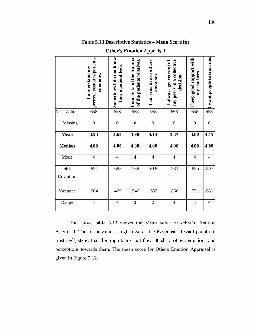
Table 5.13 Descriptive Statistics Mean Score for
I und
erst
and
my
peer
s/cla
ssm
ates
/pat
ient
s em
otio
ns.
Som
etim
es I
do n
ot k
now
ho
w a
pat
ient
feel
s.
I und
erst
and
the
trau
ma
of th
e pa
tient
s rel
ativ
es.
I am
sens
itive
to o
ther
s em
otio
ns
I alw
ays g
et c
onse
nt o
f m
y pe
ers i
n a
colle
ctiv
e de
cisio
n
I kee
p go
od r
appo
rt w
ith
my
teac
hers
.
I wan
t peo
ple
to tr
ust m
e.
N Valid 658 658 658 658 658 658 658
Missing 0 0 0 0 0 0 0
Mean 3.53 3.68 3.90 4.14 3.37 3.60 4.15
Median 4.00 4.00 4.00 4.00 4.00 4.00 4.00
Mode 4 4 4 4 4 4 4
Std.
Deviation
.951 .685 .739 .618 .931 .855 .807
Variance .904 .469 .546 .382 .866 .731 .651
Range 4 4 3 2 4 4 4
The above table 5.13 shows the Mean value of Emotion
perceptions towards them. The mean score for Others Emotion Appraisal is
given in Figure 5.12.
131
Fig 5.12 Mean Score for Others Emotion Appraisal
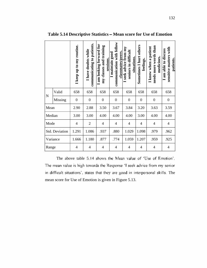
5.6.3 Use of Emotion
The Definition of Use of Emotion
use of their emotions by directing them towards constructive activities and
132
Table 5.14 Descriptive Statistics Mean score for Use of Emotion
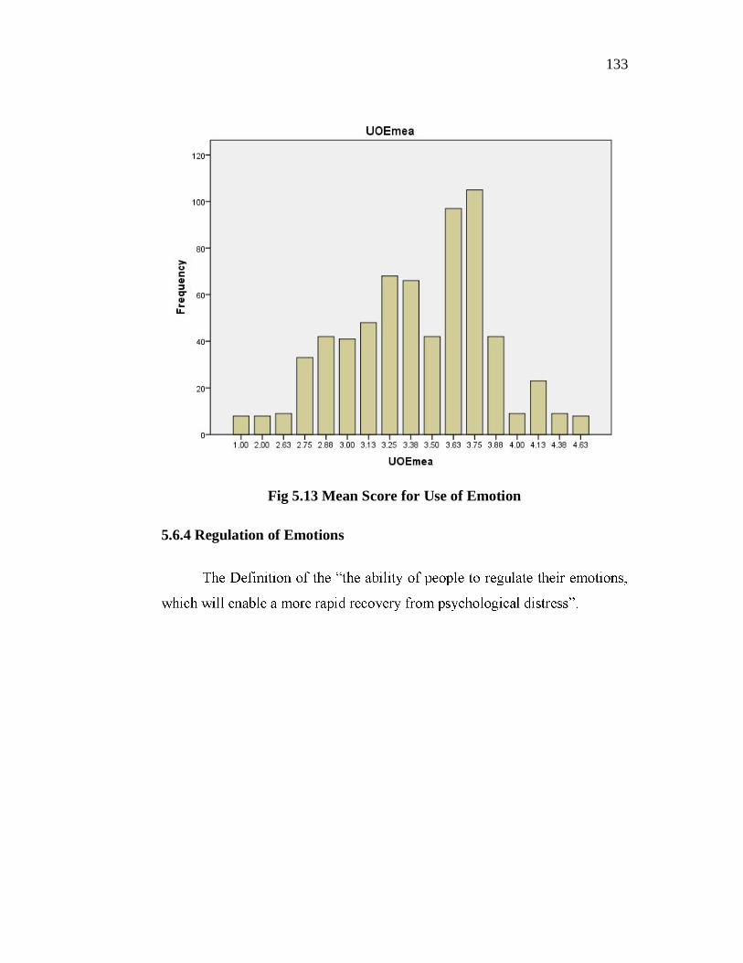
profession is high . The mean score for Regulation of Emotion is given in
Figure 5.14.
135
Fig 5.14 Mean Score for Regulation of Emotion
5.6.5 Mode and Range for Each Emotional Intelligence Factors
136
Table 5.16 Mode and Range for Each Emotional Intelligence Factors
Sl. NO Questions N
Mode Range Minimum Maximum Valid Missing
1 I understand my feelings. 658 0 4 3 2 5
2 I am happy during training sessions. 658 0 4 3 2 5
3 I enjoy my studies. 658 0 4 4 1 5
4 I want to be an ideal doctor 658 0 5 4 1 5
5 I enjoy my theory and practical sessions. 658 0 4 4 1 5
6 I understand my
peers/classmates/patients emotions.
658 0 4 4 1 5
7 Sometimes I do not know how a patient feels. 658 0 4 4 1 5
8 I understand the trauma 658 0 4 3 2 5
9 I am sensitive to others emotions 658 0 4 2 3 5
10 I always get consent of my peers in a collective
decision 658 0 4 4 1 5
137
11 I keep good rapport with my teachers. 658 0 4 4 1 5
12 I want people to trust me. 658 0 4 4 1 5
13 I keep up to my routine. 658 0 4 4 1 5
14 I have doubts while communicating to
patients. 658 0 2 4 1 5
15 I am looking forward for my classes and training
sessions. 658 0 4 4 1 5
16 I maintain good
communication with fellow classmates/peers.
658 0 4 4 1 5
17 I seek advice from my
seniors in difficult situations.
658 0 4 4 1 5
18 Sometimes I hurt others feelings. 658 0 4 4 1 5
19 I know when a patient
needs more words than medicines.
658 0 4 4 1 5
138
20 I am able to discuss
sensitive matters with patients.
658 0 4 4 1 5
21 I know what triggers my emotions. 658 0 4 4 1 5
22 I know when I am stressed. 658 0 4 4 1 5
23 I help people when they are in need. 658 0 4 4 1 5
24 I take responsibility of my decisions. 658 0 4 3 2 5
25 I finish my assignments on time. 658 0 4 4 1 5
26 I take responsibility for my emotions. 658 0 4 4 1 5
27 I manage mine as well as
others emotions simultaneously.
658 0 4 4 1 5
28 I keep myself cool during emergencies. 658 0 4 4 1 5
29 I always make sure that
others do not misunderstand me.
658 0 4 4 1 5
139
30 I am always open for discussions. 658 0 4 4 1 5
31 I will not put myself in an embarrassing situation 658 0 4 4 1 5
32 I will see that my patients are not very emotional. 658 0 4 3 2 5
33 I idealize myself to be a trustworthy person. 658 0 4 3 2 5
The above table 5.16 shows the value of mode and Range towards the
Emotional Intelligence factors. The Mode is the Score that Occurs Often. The Data
is normally distributed having the Mode value =4, states that there is equal
distribution among the Variables and Frequently Occurs in the distribution.
5.6.6 T Test:
Table 5.17 Mean score for Dimensions of Emotional Intelligence
T- Value =3.70
N Mean Std. Deviation T-Value P-Value
SEA 658 3.83 .584 5.754 .000
OEA 658 3.77 .476 3.615 .000
UOE 658 3.40 .506 -15.137 .000
ROE 658 3.64 .475 -3.362 .001
140
The above table 5.17 shows the value of T Test, having the T value
3.70, which states that level of EI is medium. From the table it is inferred that
, the EI factors lies in the range of 3.70, and the Significance P- value is less
than the Alpha value states there is Significant difference between the SEA,
OEA, UOE and ROE Factors of EI.
5.7. TO ASSESS THE IMPACT OF AGE ON THE LEVEL OF
EMOTIONAL INTELLIGENCE AMONG THE MEDICAL
STUDENTS.
Table 5.18 Cross tabulation for Age and EI level towards
the Self Emotion Appraisal
SEA Mean
Value Total Medium High
Age of the respondents
20 25 years
Count 66 465 531 Expected Count 79.1 451.9 531.0 % within Age of the respondents
12.4% 87.6% 100.0%
26 - 30 years
Count 32 42 74 Expected Count 11.0 63.0 74.0 % within Age of the respondents
43.2% 56.8% 100.0%
31 35 years
Count 0 53 53 Expected Count 7.9 45.1 53.0 % within Age of the respondents
.0% 100.0% 100.0%
Total Count 98 560 658 Expected Count 98.0 560.0 658.0 % within Age of the respondents
14.9% 85.1% 100.0%
141
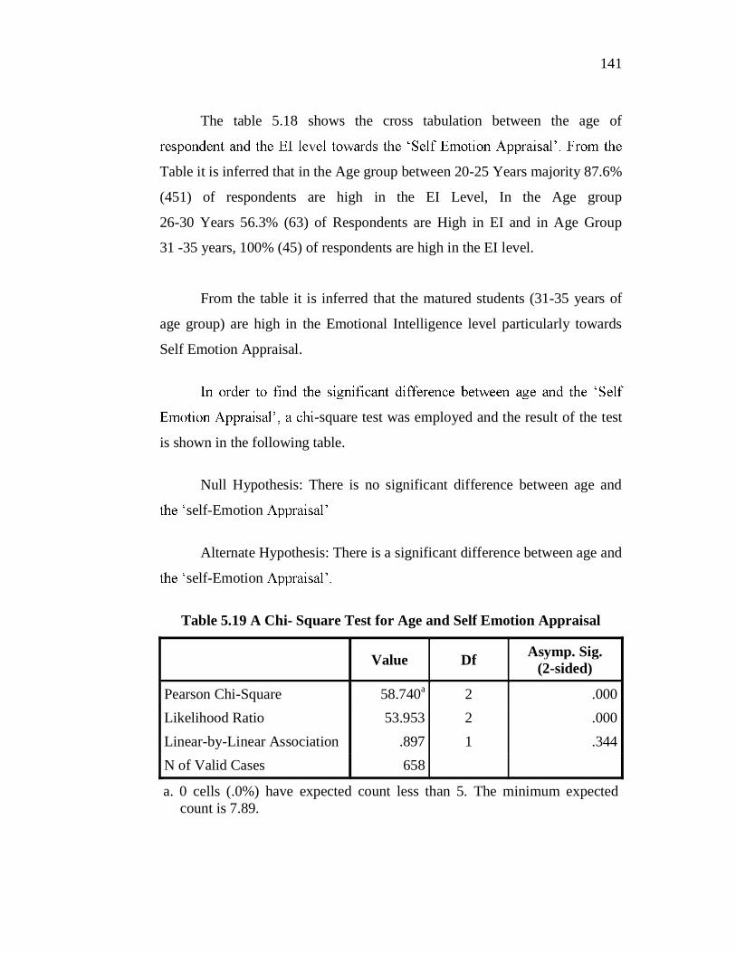
The table 5.18 shows the cross tabulation between the age of
Table it is inferred that in the Age group between 20-25 Years majority 87.6%
(451) of respondents are high in the EI Level, In the Age group
26-30 Years 56.3% (63) of Respondents are High in EI and in Age Group
31 -35 years, 100% (45) of respondents are high in the EI level.
From the table it is inferred that the matured students (31-35 years of
age group) are high in the Emotional Intelligence level particularly towards
Self Emotion Appraisal.
-square test was employed and the result of the test
is shown in the following table.
Null Hypothesis: There is no significant difference between age and
self-Emotion
Alternate Hypothesis: There is a significant difference between age and
self-Emotion
Table 5.19 A Chi- Square Test for Age and Self Emotion Appraisal
Value Df Asymp. Sig. (2-sided)
Pearson Chi-Square 58.740a 2 .000 Likelihood Ratio 53.953 2 .000 Linear-by-Linear Association .897 1 .344 N of Valid Cases 658
a. 0 cells (.0%) have expected count less than 5. The minimum expected count is 7.89.
142
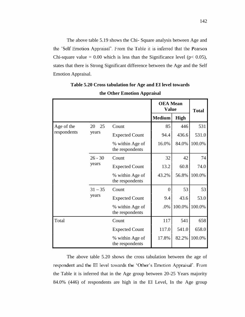
The above table 5.19 shows the Chi- Square analysis between Age and
Chi-square value = 0.00 which is less than the Significance level (p< 0.05),
states that there is Strong Significant difference between the Age and the Self
Emotion Appraisal.
Table 5.20 Cross tabulation for Age and EI level towards
the Other Emotion Appraisal
OEA Mean
Value Total Medium High
Age of the respondents
20 25 years
Count 85 446 531
Expected Count 94.4 436.6 531.0
% within Age of the respondents
16.0% 84.0% 100.0%
26 - 30 years
Count 32 42 74
Expected Count 13.2 60.8 74.0
% within Age of the respondents
43.2% 56.8% 100.0%
31 35 years
Count 0 53 53
Expected Count 9.4 43.6 53.0
% within Age of the respondents
.0% 100.0% 100.0%
Total Count 117 541 658
Expected Count 117.0 541.0 658.0
% within Age of the respondents
17.8% 82.2% 100.0%
The above table 5.20 shows the cross tabulation between the age of
the Table it is inferred that in the Age group between 20-25 Years majority
84.0% (446) of respondents are high in the EI Level, In the Age group
143
26-30 Years 56.8% (42) of Respondents are High in EI and in Age Group
31 -35 years, 100% (53) of respondents are high in the EI level.
From the table it is inferred that the matured students (31-35 years of
age group) are high in the Emotional Intelligence level particularly towards
-square test was employed and the result of the test
is shown in the following table.
Null Hypothesis: There is no significant difference between age and
Alternate Hypothesis: There is a significant difference between age and
Table 5.21 A Chi- s Emotion Appraisal
Value Df Asymp. Sig.
(2-sided)
Pearson Chi-Square 45.421a 2 .000
Likelihood Ratio 47.673 2 .000
Linear-by-Linear Association .000 1 .999
N of Valid Cases 658
a. 0 cells (.0%) have expected count less than 5. The minimum expected count is 9.42.
The above table 5.21 shows the Chi- Square analysis between Age and
Pearson Chi-square value = 0.00 which is less than the Significance level
(p< 0.05), states that there is Strong Significant difference between the Age
144
Table 5.22 Cross tabulation for Age and EI level towards
the Use of Emotion Appraisal
UOE Mean Value
Total Low Medium High
Age of the respondents
20 25 years
Count 8 216 307 531
Expected Count 6.5 200.9 323.6 531.0
% within Age of the respondents
1.5% 40.7% 57.8% 100.0%
26 - 30 years
Count 0 24 50 74
Expected Count .9 28.0 45.1 74.0
% within Age of the respondents
.0% 32.4% 67.6% 100.0%
31 35 years
Count 0 9 44 53
Expected Count .6 20.1 32.3 53.0
% within Age of the respondents
.0% 17.0% 83.0% 100.0%
Total Count 8 249 401 658
Expected Count 8.0 249.0 401.0 658.0
% within Age of the respondents
1.2% 37.8% 60.9% 100.0%
The above table 5.22 shows the cross tabulation between the age of
. From the Table it
is inferred that in the Age group between 20-25 Years majority 57.8% (307)
of respondents are high in the EI Level, In the Age group 26-30 Years 67.6%
(50) of Respondents are High in EI and in Age Group 31 -35 years, 83% (44)
of respondents are high in the EI level.
145
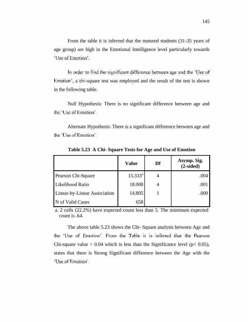
From the table it is inferred that the matured students (31-35 years of
age group) are high in the Emotional Intelligence level particularly towards
.
-square test was employed and the result of the test is shown
in the following table.
Null Hypothesis: There is no significant difference between age and
Alternate Hypothesis: There is a significant difference between age and
Table 5.23 A Chi- Square Tests for Age and Use of Emotion
Value Df Asymp. Sig. (2-sided)
Pearson Chi-Square 15.333a 4 .004
Likelihood Ratio 18.008 4 .001
Linear-by-Linear Association 14.805 1 .000
N of Valid Cases 658 a. 2 cells (22.2%) have expected count less than 5. The minimum expected
count is .64.
The above table 5.23 shows the Chi- Square analysis between Age and
Chi-square value = 0.04 which is less than the Significance level (p< 0.05),
states that there is Strong Significant difference between the Age with the
146
Table 5.24 Cross tabulation for Age and EI level towards the
Regulation of Emotion
ROE Mean
Value
Total Medium High
Age of the respondents
20 25 years
Count 132 399 531
Expected Count 125.9 405.1 531.0
% within Age of the respondents
24.9% 75.1% 100.0%
26 - 30 years
Count 24 50 74
Expected Count 17.5 56.5 74.0
% within Age of the respondents
32.4% 67.6% 100.0%
31 35 years
Count 0 53 53
Expected Count 12.6 40.4 53.0
% within Age of the respondents
.0% 100.0% 100.0%
Total Count 156 502 658
Expected Count 156.0 502.0 658.0
% within Age of the respondents
23.7% 76.3% 100.0%
1
The above table 5.24 shows the cross tabulation between the age of
Table it is inferred that in the Age group between 20-25 Years majority
75.1% (399) of respondents are high in the EI Level, In the Age group
26-30 Years 67.6% (50) of Respondents are High in EI and in Age Group
31 -35 years, 100% (53) of respondents are high in the EI level.
147
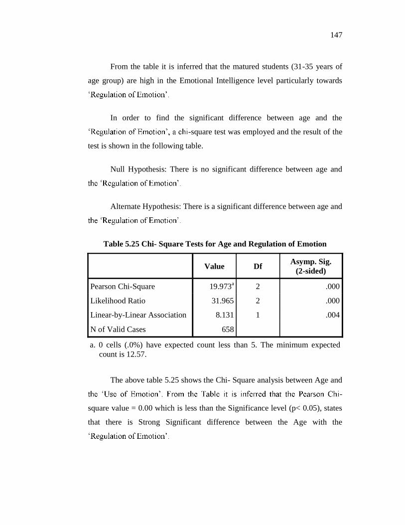
From the table it is inferred that the matured students (31-35 years of
age group) are high in the Emotional Intelligence level particularly towards
In order to find the significant difference between age and the
-square test was employed and the result of the
test is shown in the following table.
Null Hypothesis: There is no significant difference between age and
Alternate Hypothesis: There is a significant difference between age and
Table 5.25 Chi- Square Tests for Age and Regulation of Emotion
Value Df Asymp. Sig. (2-sided)
Pearson Chi-Square 19.973a 2 .000
Likelihood Ratio 31.965 2 .000
Linear-by-Linear Association 8.131 1 .004
N of Valid Cases 658
a. 0 cells (.0%) have expected count less than 5. The minimum expected count is 12.57.
The above table 5.25 shows the Chi- Square analysis between Age and
-
square value = 0.00 which is less than the Significance level (p< 0.05), states
that there is Strong Significant difference between the Age with the
148
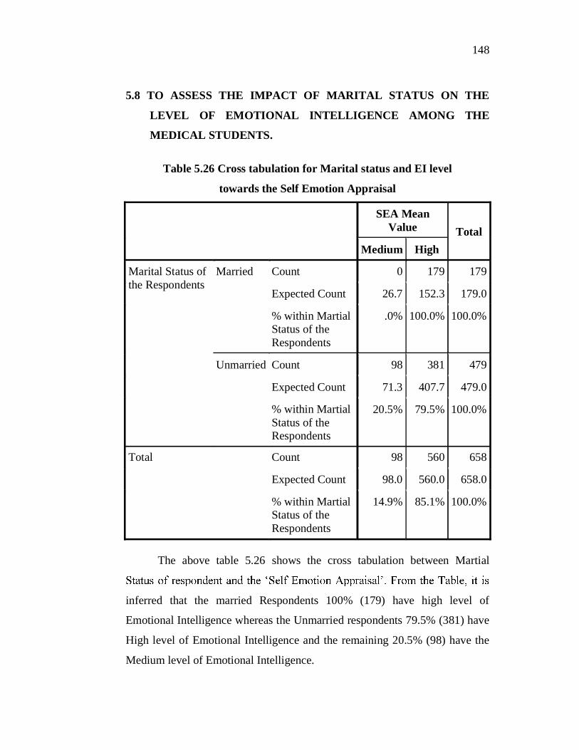
5.8 TO ASSESS THE IMPACT OF MARITAL STATUS ON THE
LEVEL OF EMOTIONAL INTELLIGENCE AMONG THE
MEDICAL STUDENTS.
Table 5.26 Cross tabulation for Marital status and EI level
towards the Self Emotion Appraisal
SEA Mean
Value Total Medium High
Marital Status of the Respondents
Married Count 0 179 179
Expected Count 26.7 152.3 179.0
% within Martial Status of the Respondents
.0% 100.0% 100.0%
Unmarried Count 98 381 479
Expected Count 71.3 407.7 479.0
% within Martial Status of the Respondents
20.5% 79.5% 100.0%
Total Count 98 560 658
Expected Count 98.0 560.0 658.0
% within Martial Status of the Respondents
14.9% 85.1% 100.0%
The above table 5.26 shows the cross tabulation between Martial
inferred that the married Respondents 100% (179) have high level of
Emotional Intelligence whereas the Unmarried respondents 79.5% (381) have
High level of Emotional Intelligence and the remaining 20.5% (98) have the
Medium level of Emotional Intelligence.
149
From the table it is inferred that the married respondents have high
In order to find the significant difference between marital status and
-square test was employed and the result of
the test is shown in the following table.
Null Hypothesis: There is no significant difference between Marital
Alternate Hypothesis: There is a significant difference between Marital
Table 5.27 A Chi-Square Tests for Marital status and
the Self Emotion Appraisal
Value Df Asymp.
Sig. (2-sided)
Exact Sig. (2-sided)
Exact Sig. (1-sided)
Pearson Chi-Square 43.031a 1 .000
Continuity Correction
41.432 1 .000
Likelihood Ratio 68.428 1 .000
Fisher's Exact Test .000 .000
Linear-by-Linear Association
42.966 1 .000
N of Valid Cases 658
a. 0 cells (.0%) have expected count less than 5. The minimum expected count is 26.66.
b. Computed only for a 2x2 table The above table 5.27 shows the Chi- Square analysis between Marital
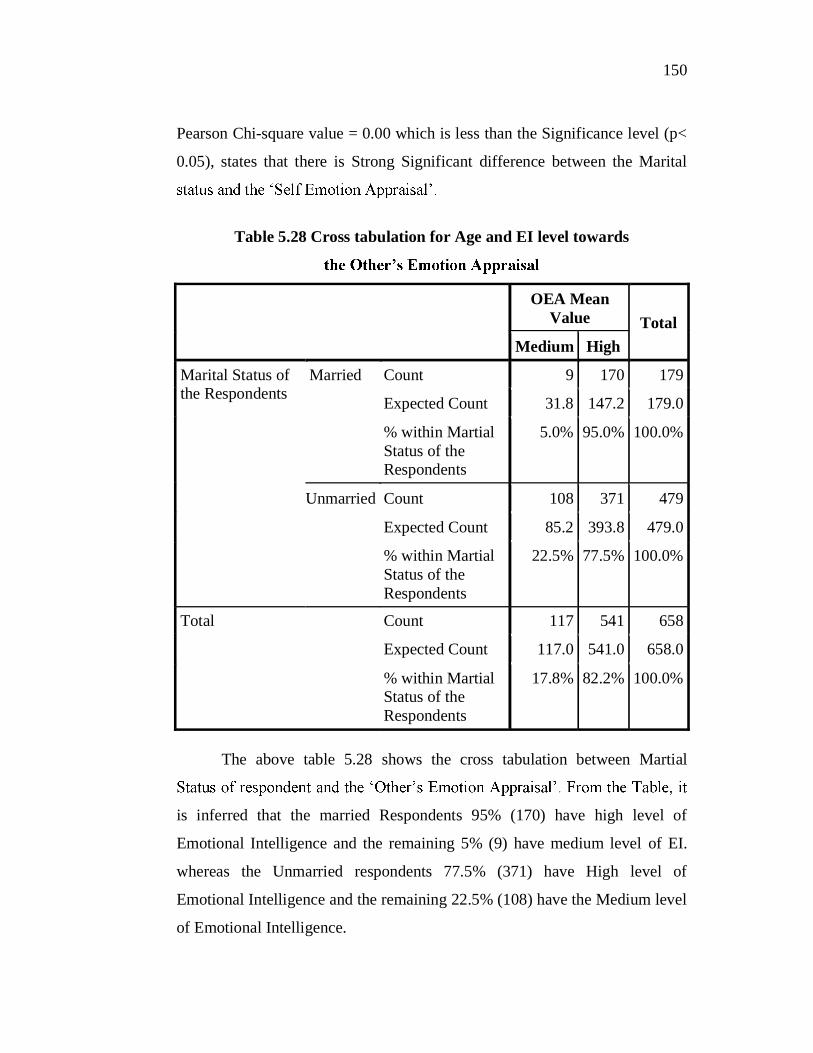
150
Pearson Chi-square value = 0.00 which is less than the Significance level (p<
0.05), states that there is Strong Significant difference between the Marital
Table 5.28 Cross tabulation for Age and EI level towards
OEA Mean
Value Total Medium High
Marital Status of the Respondents
Married Count 9 170 179
Expected Count 31.8 147.2 179.0
% within Martial Status of the Respondents
5.0% 95.0% 100.0%
Unmarried Count 108 371 479
Expected Count 85.2 393.8 479.0
% within Martial Status of the Respondents
22.5% 77.5% 100.0%
Total Count 117 541 658
Expected Count 117.0 541.0 658.0
% within Martial Status of the Respondents
17.8% 82.2% 100.0%
The above table 5.28 shows the cross tabulation between Martial
is inferred that the married Respondents 95% (170) have high level of
Emotional Intelligence and the remaining 5% (9) have medium level of EI.
whereas the Unmarried respondents 77.5% (371) have High level of
Emotional Intelligence and the remaining 22.5% (108) have the Medium level
of Emotional Intelligence.
151
From the table it is inferred that the married respondents have high
level of Emo
In order to find the significant difference between marital status and
-square test was employed and the
result of the test is shown in the following table.
Null Hypothesis: There is no significant difference between Marital
Alternate Hypothesis: There is a significant difference between Marital
Table 5.29 A Chi-Square Tests for Marital status and
Value df Asymp.
Sig. (2-sided)
Exact Sig. (2-sided)
Exact Sig. (1-sided)
Pearson Chi-Square 27.356a 1 .000
Continuity Correctionb
26.171 1 .000
Likelihood Ratio 33.276 1 .000
Fisher's Exact Test .000 .000
Linear-by-Linear Association
27.314 1 .000
N of Valid Cases 658
a. 0 cells (.0%) have expected count less than 5. The minimum expected count is 31.83.
b. Computed only for a 2x2 table
152
The above table 5.29 shows the Chi- Square analysis between Marital
the Pearson Chi-square value = 0.00 which is less than the Significance level
(p< 0.05), states that there is Strong Significant difference between the
Marital status and t
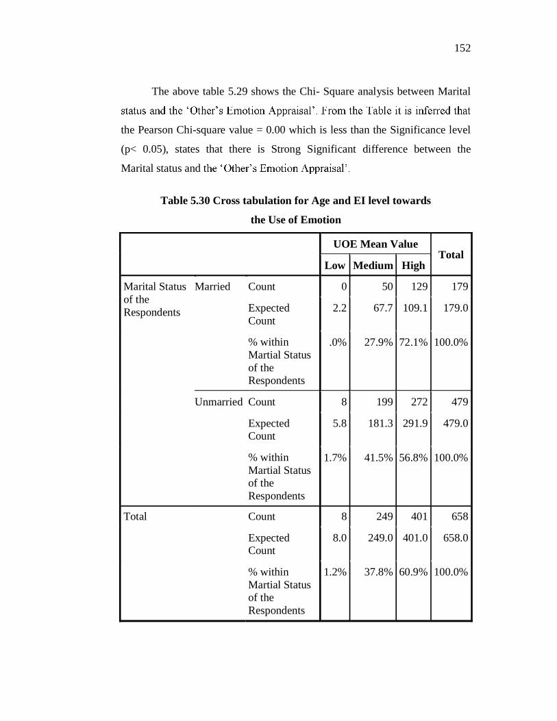
Table 5.30 Cross tabulation for Age and EI level towards
the Use of Emotion
UOE Mean Value
Total Low Medium High
Marital Status of the Respondents
Married Count 0 50 129 179
Expected Count
2.2 67.7 109.1 179.0
% within Martial Status of the Respondents
.0% 27.9% 72.1% 100.0%
Unmarried Count 8 199 272 479
Expected Count
5.8 181.3 291.9 479.0
% within Martial Status of the Respondents
1.7% 41.5% 56.8% 100.0%
Total Count 8 249 401 658
Expected Count
8.0 249.0 401.0 658.0
% within Martial Status of the Respondents
1.2% 37.8% 60.9% 100.0%
153
The above table 5.30 shows the cross tabulation between Martial
ium
Whereas the Unmarried respondents 56.8% (272) have high EI in Use
of Emotion and 41.5% (199) of respondents have medium Ei in Use of
emotion and the remaining 1.7% (8) have low EI in Use of emotion.
From the table it is inferred that the married respondents have high
In order to find the significant difference between marital status and
-square test was employed and the result of the test
is shown in the following table.
Null Hypothesis: There is no significant difference between Marital
Alternate Hypothesis: There is a significant difference between Marital
Table 5.31 A Chi-Square Tests for Marital status
and the Use of Emotion
Value Df Asymp. Sig. (2-sided)
Pearson Chi-Square 14.363a 2 .001 Likelihood Ratio 16.697 2 .000 Linear-by-Linear Association 14.117 1 .000 N of Valid Cases 658 a. 1 cells (16.7%) have expected count less than 5. The minimum expected
count is 2.18.
154
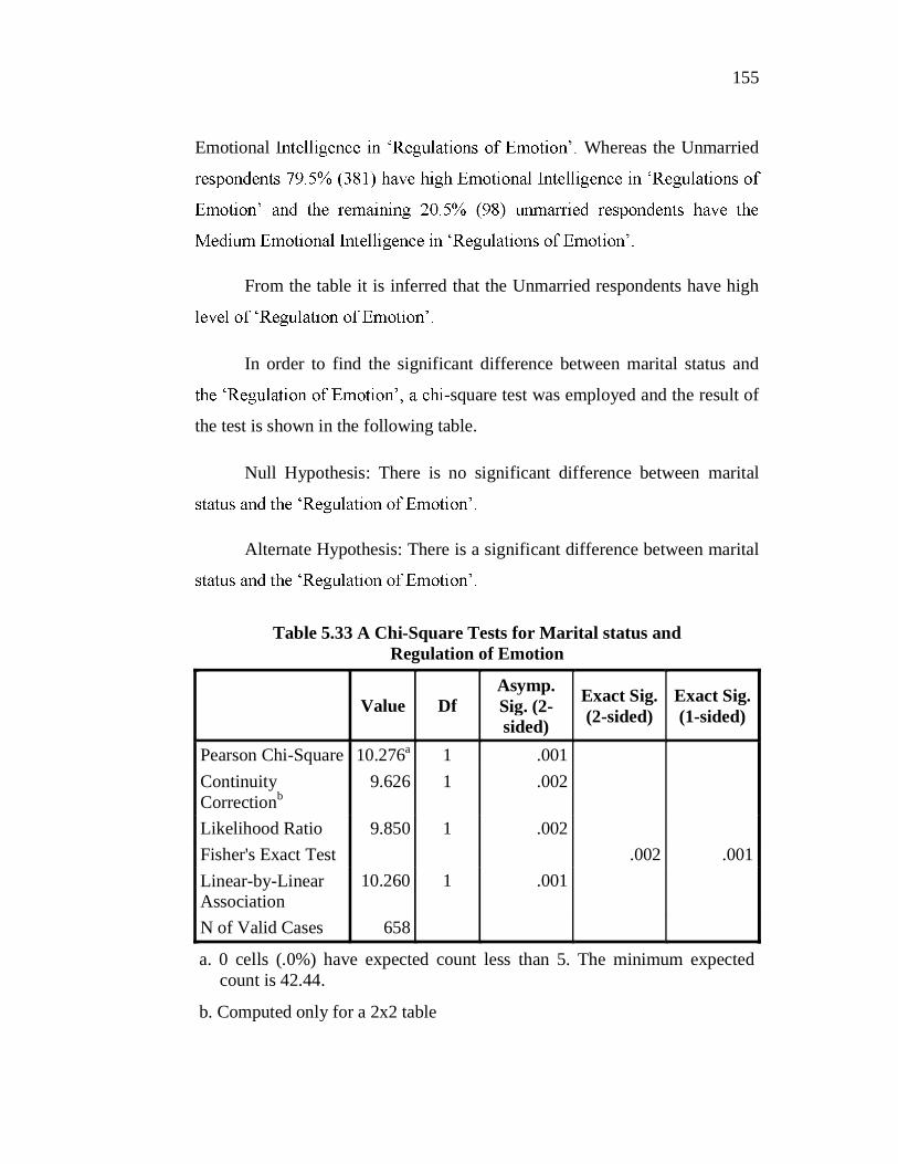
The above table 5.31 shows the Chi- Square analysis between Marital
. From the Table it is inferred that the Pearson
Chi-square value = 0.001 which is less than the Significance level (p< 0.05),
states that there is Strong Significant difference between the Marital status
Table 5.32 Cross tabulation for Age and EI level towards
the Regulation of Emotion
ROE Mean
Value Total Medium High
Marital Status of the Respondents
Married Count 58 121 179
Expected Count 42.4 136.6 179.0
% within Martial Status of the Respondents
32.4% 67.6% 100.0%
Unmarried Count 98 381 479
Expected Count 113.6 365.4 479.0
% within Martial Status of the Respondents
20.5% 79.5% 100.0%
Total Count 156 502 658
Expected Count 156.0 502.0 658.0
% within Martial Status of the Respondents
23.7% 76.3% 100.0%
The above table 5.32 shows the cross tabulation between Martial
Status and the Regulation of Emotions. From the Table, it is inferred that the
married Respondents 67.6% (121) have high Emotional Intelligence in
medium
155
Emotional Whereas the Unmarried
From the table it is inferred that the Unmarried respondents have high
In order to find the significant difference between marital status and
-square test was employed and the result of
the test is shown in the following table. Null Hypothesis: There is no significant difference between marital
Alternate Hypothesis: There is a significant difference between marital
Table 5.33 A Chi-Square Tests for Marital status and Regulation of Emotion