Applied Computational Fluid Dynamics Computer-Aided Analysis on Energy ad Thermofluid Sciences Part I: Introduction and Governing Equations Instructor: Professor Yang-Cheng Shih Department of Energy and Refrigerating Air-Conditioning Engineering National Taipei University of Technology September 2013
Transcript
Applied Computational Fluid Dynamics
Computer-Aided Analysis on Energy ad
Thermofluid Sciences
Part I: Introduction and Governing Equations
Instructor: Professor Yang-Cheng Shih Department of Energy and Refrigerating Air-Conditioning Engineering
National Taipei University of Technology
September 2013
Applied Computational Fluid Dynamics
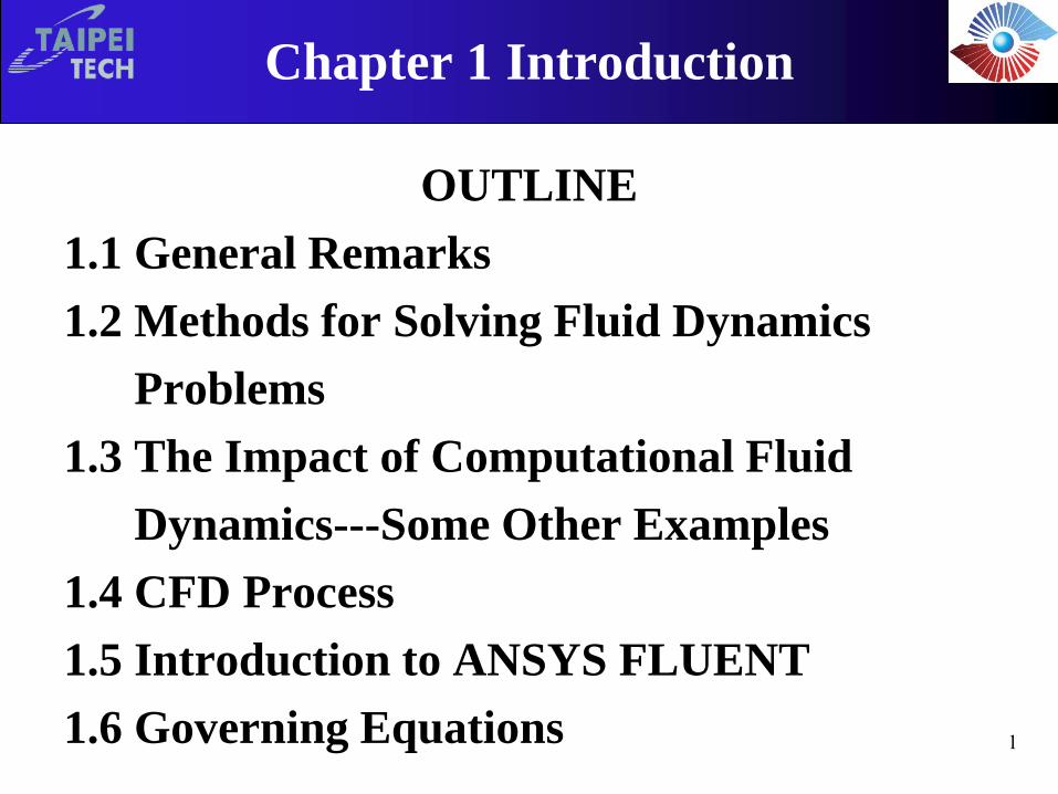
Chapter 1 Introduction
OUTLINE
1.1 General Remarks
1.2 Methods for Solving Fluid Dynamics
Problems
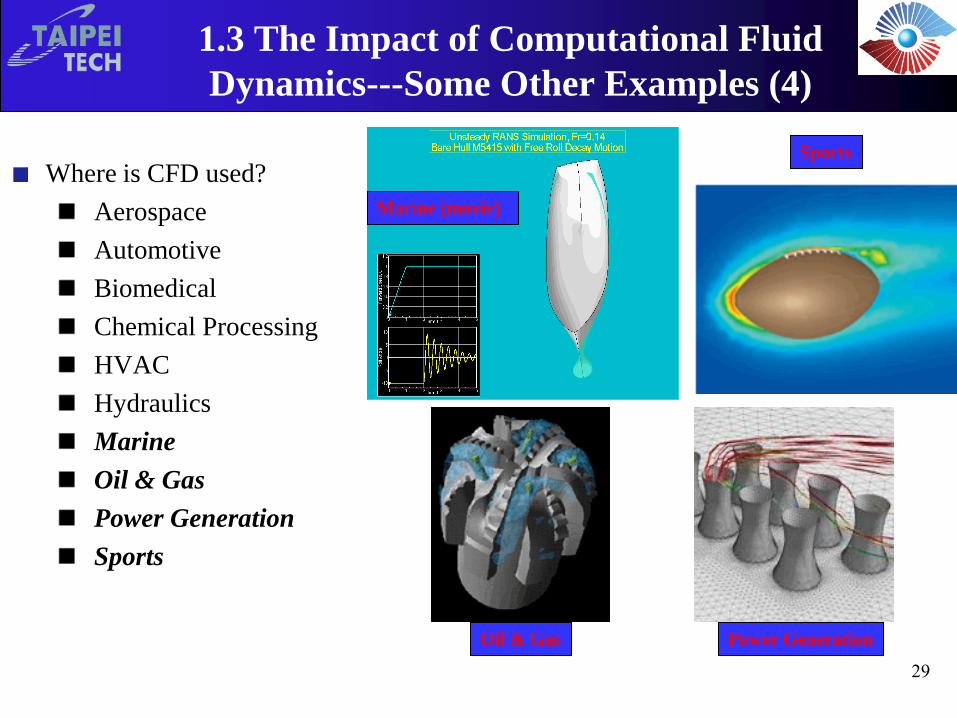
1.3 The Impact of Computational Fluid
Dynamics---Some Other Examples
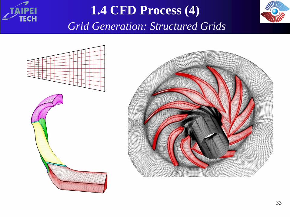
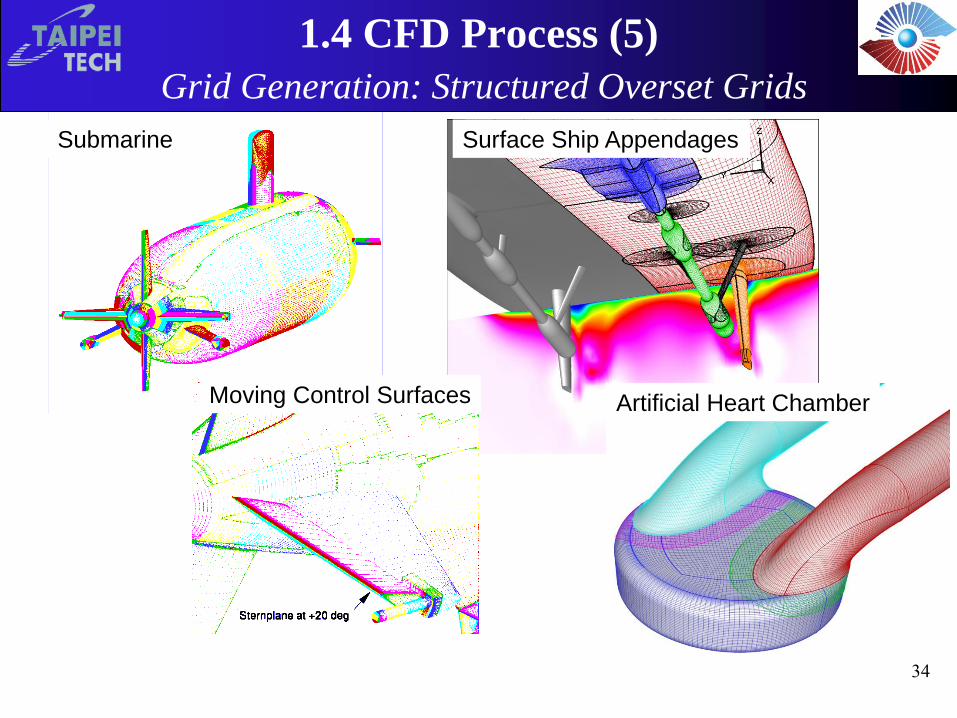
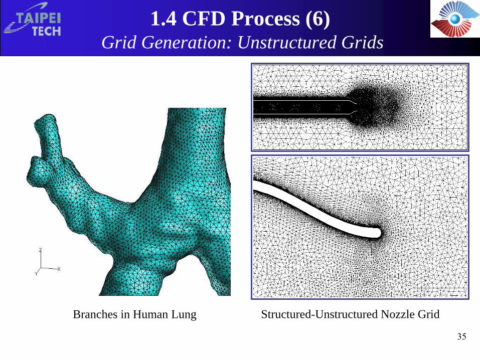
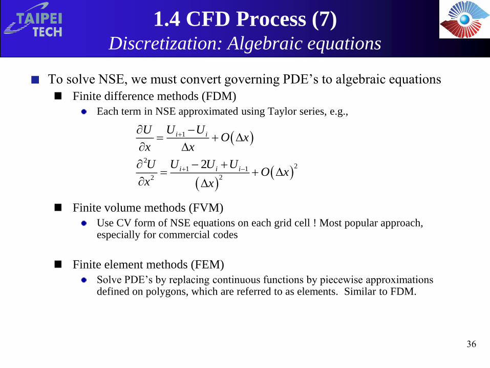
1.4 CFD Process
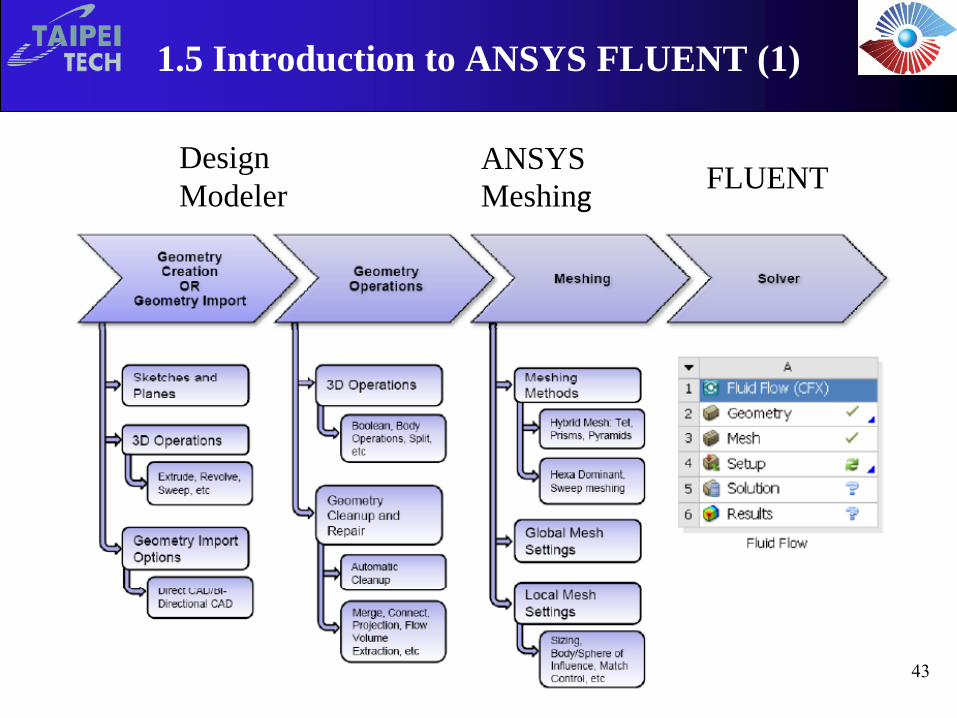
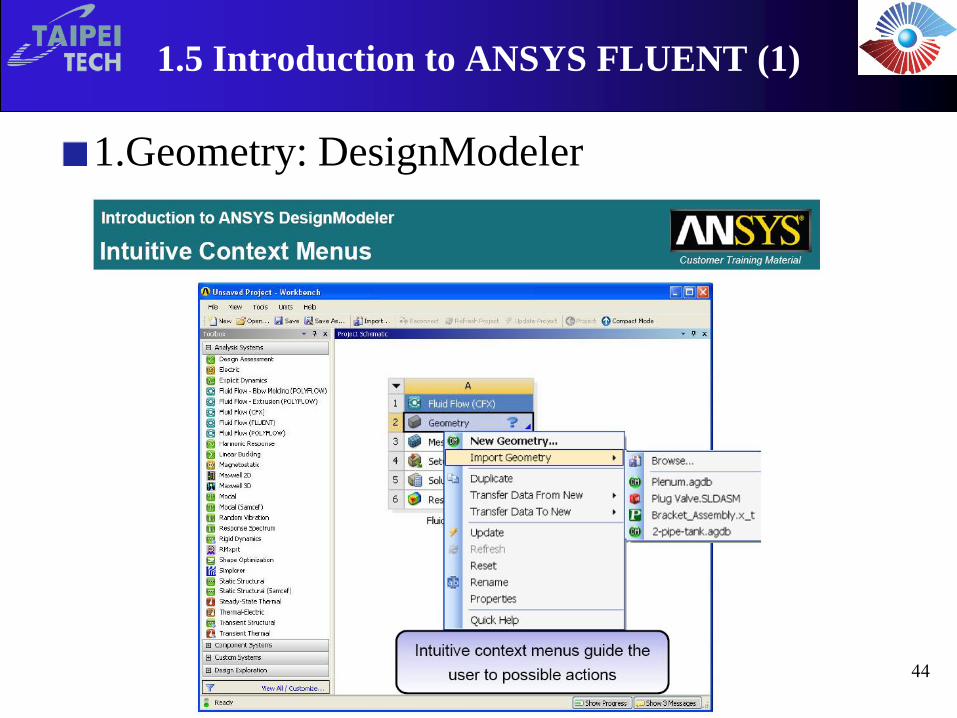
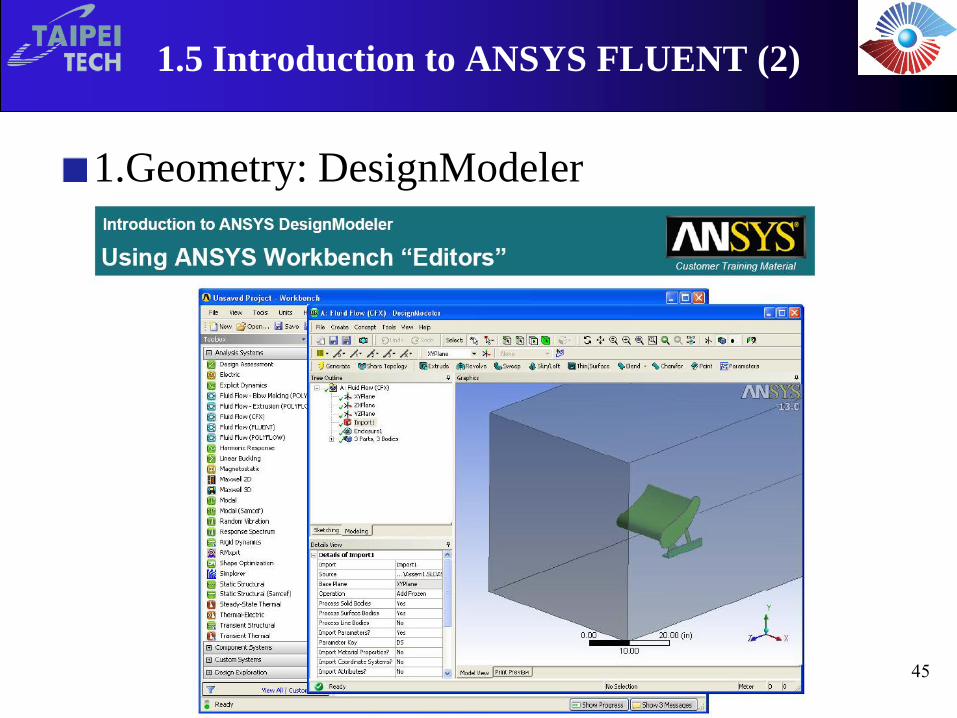
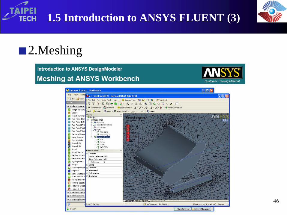
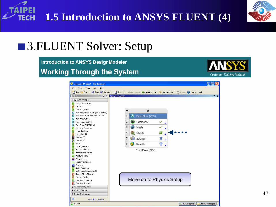
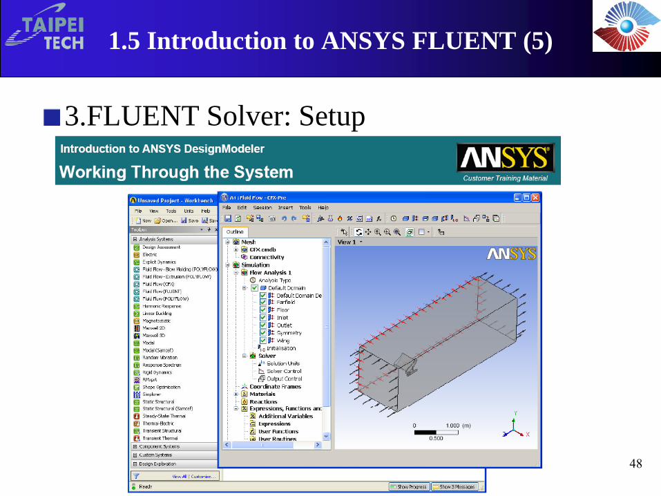
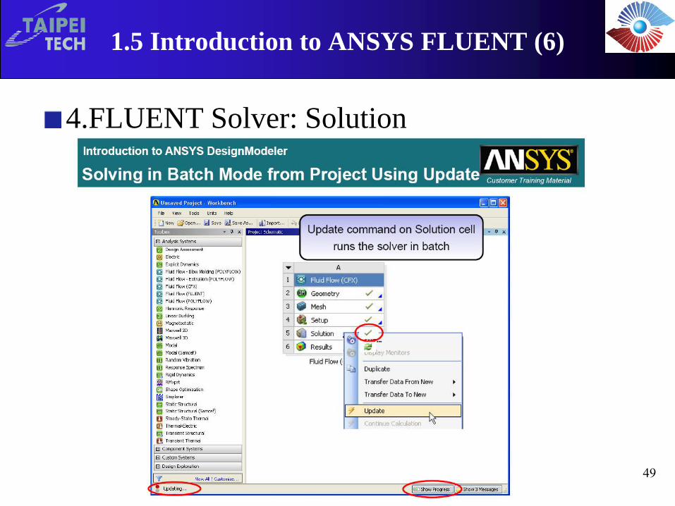
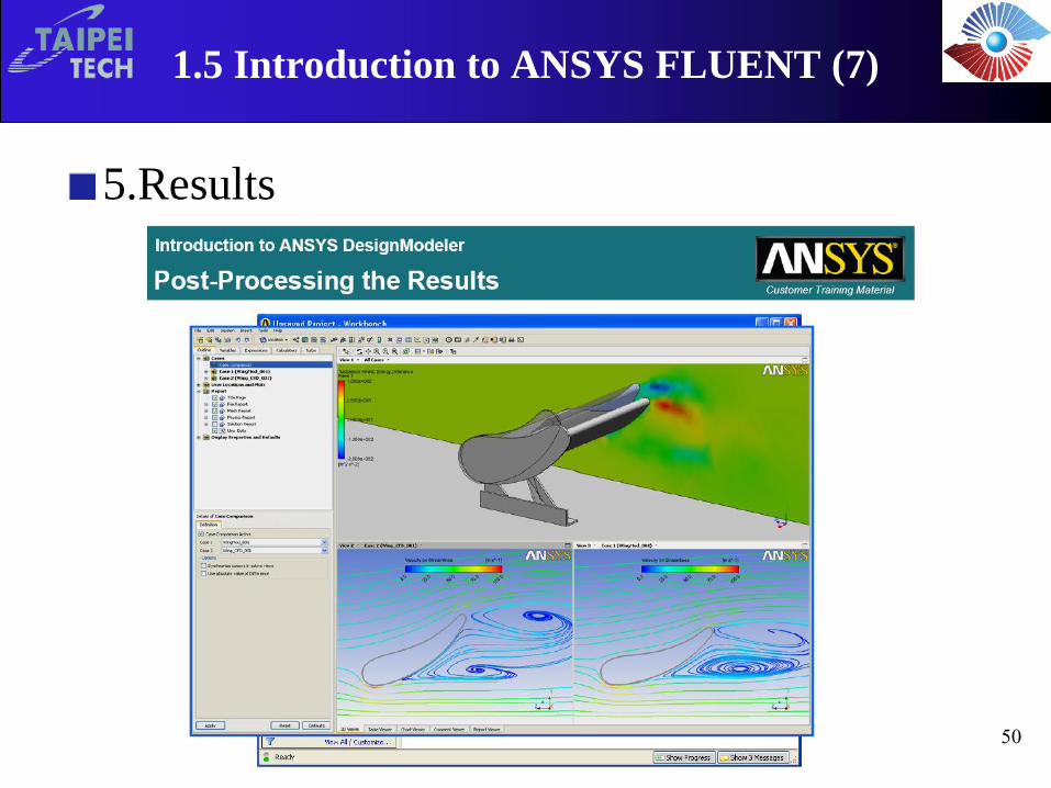
1.5 Introduction to ANSYS FLUENT
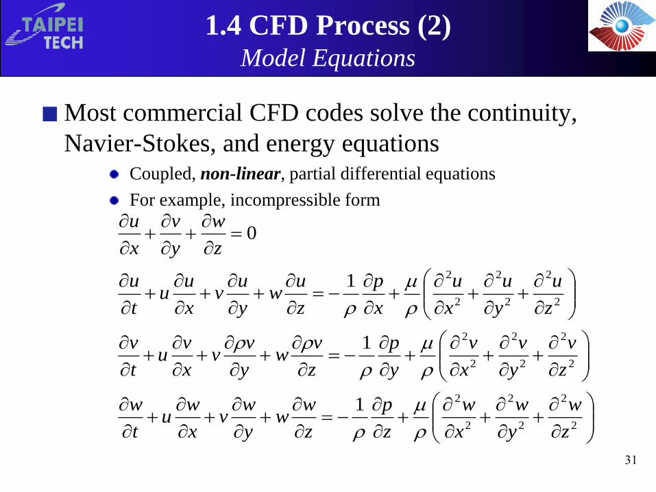
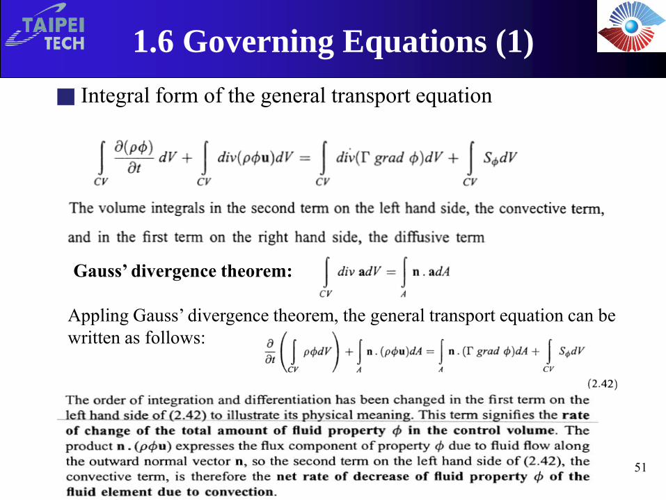
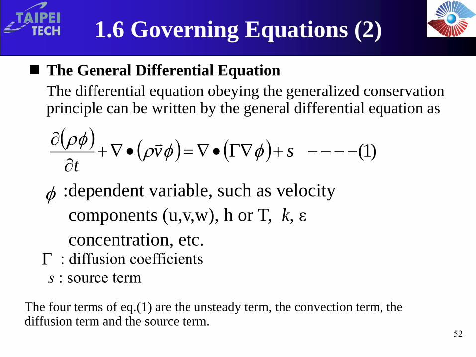
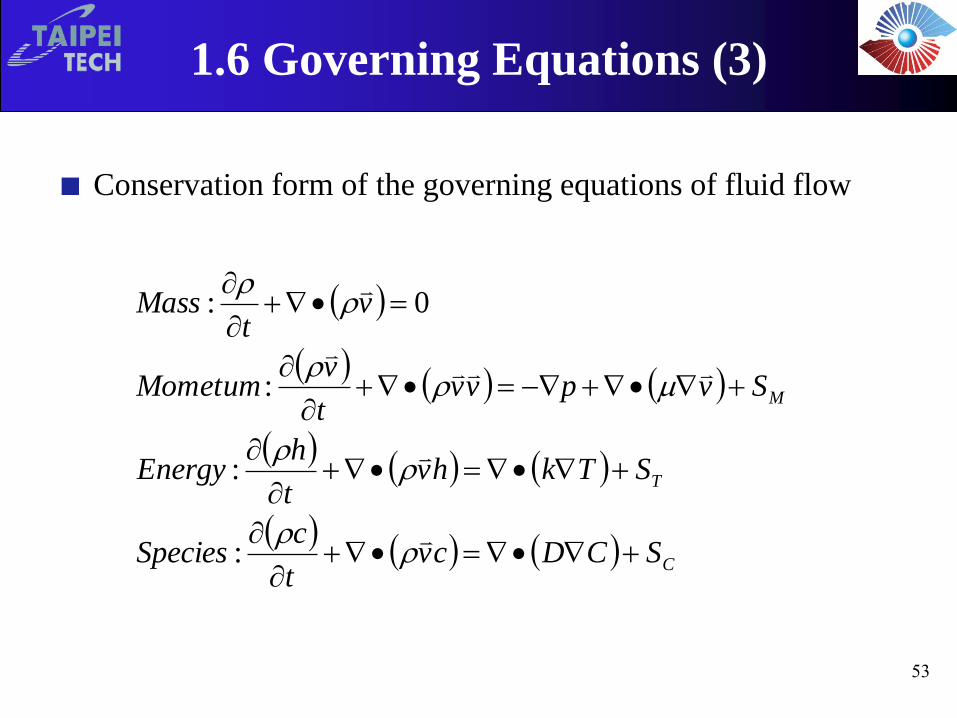
1.6 Governing Equations
1
Applied Computational Fluid Dynamics
1.1 General Remarks (1)
Preface
Practice of engineering and science has been dramatically altered by the development of
Scientific computing
Mathematics of numerical analysis
The Internet
Computational Fluid Dynamics is based upon the logic of applied mathematics
provides tools to unlock previously unsolved problems
is used in nearly all fields of science and engineering
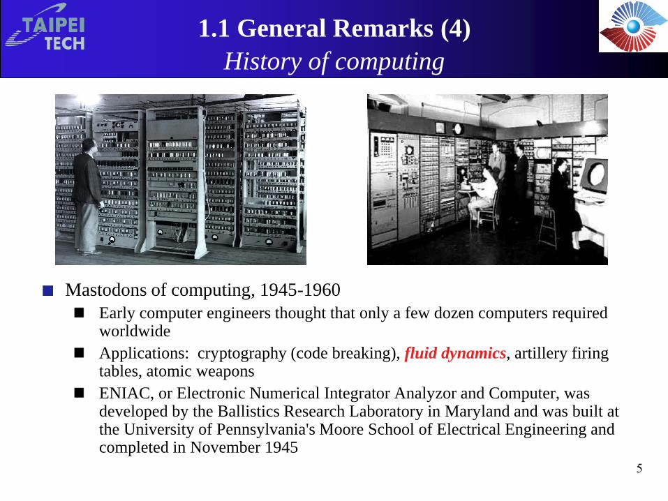
ENIAC, or Electronic Numerical Integrator Analyzor and Computer, was developed by the Ballistics Research Laboratory in Maryland and was built at the University of Pennsylvania's Moore School of Electrical Engineering and completed in November 1945
5
Applied Computational Fluid Dynamics
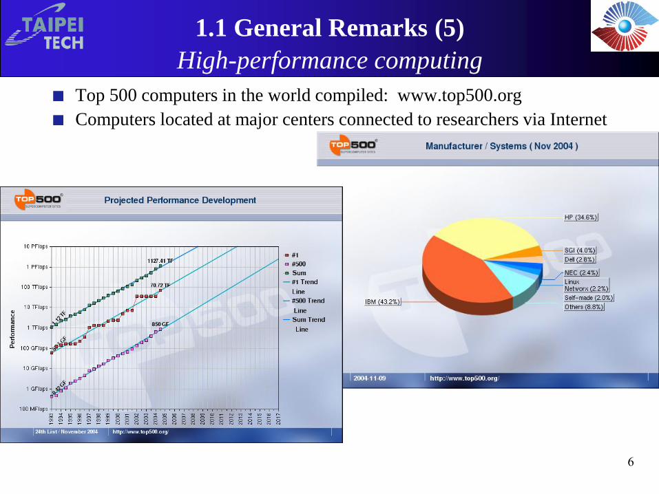
1.1 General Remarks (5) High-performance computing
Top 500 computers in the world compiled: www.top500.org
Computers located at major centers connected to researchers via Internet
6
Applied Computational Fluid Dynamics
1.1 General Remarks (6) Motivation for Studying Fluid Mechanics
Fluid Mechanics is omnipresent
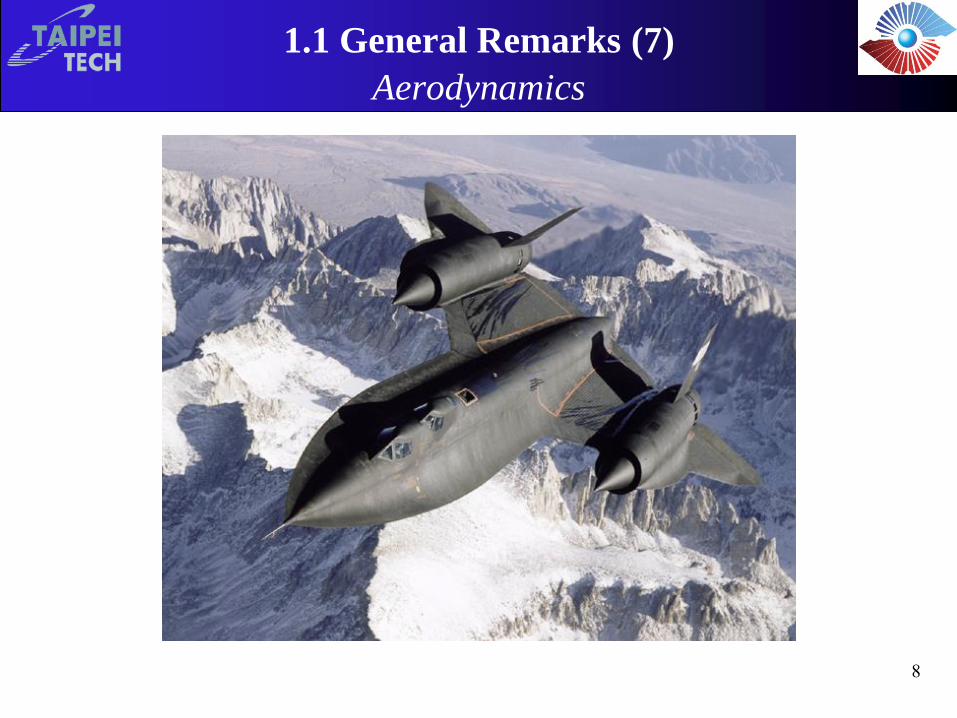
Aerodynamics
Bioengineering and biological systems
Energy generation
Geology
Hydraulics and Hydrology
Hydrodynamics
Meteorology
Ocean and Coastal Engineering
Water Resources
…numerous other examples…
7
Applied Computational Fluid Dynamics
1.1 General Remarks (7) Aerodynamics
8
Applied Computational Fluid Dynamics
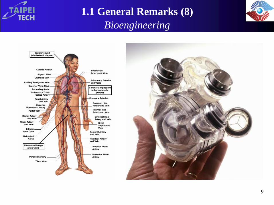
1.1 General Remarks (8) Bioengineering
9
Applied Computational Fluid Dynamics
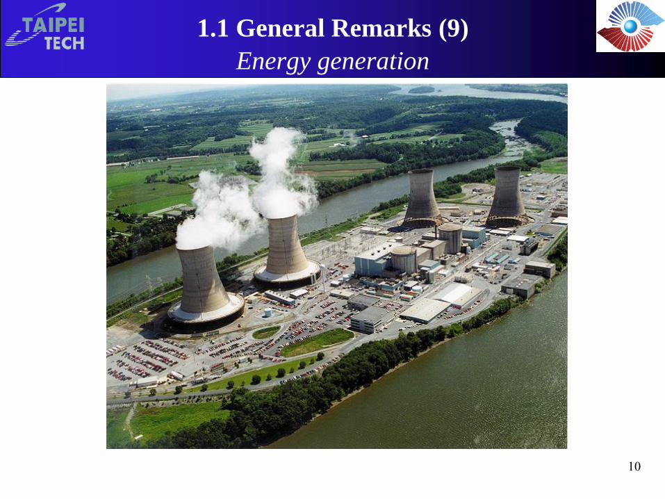
1.1 General Remarks (9) Energy generation
10
Applied Computational Fluid Dynamics
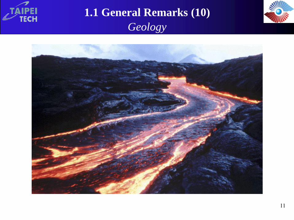
1.1 General Remarks (10) Geology
11
Applied Computational Fluid Dynamics
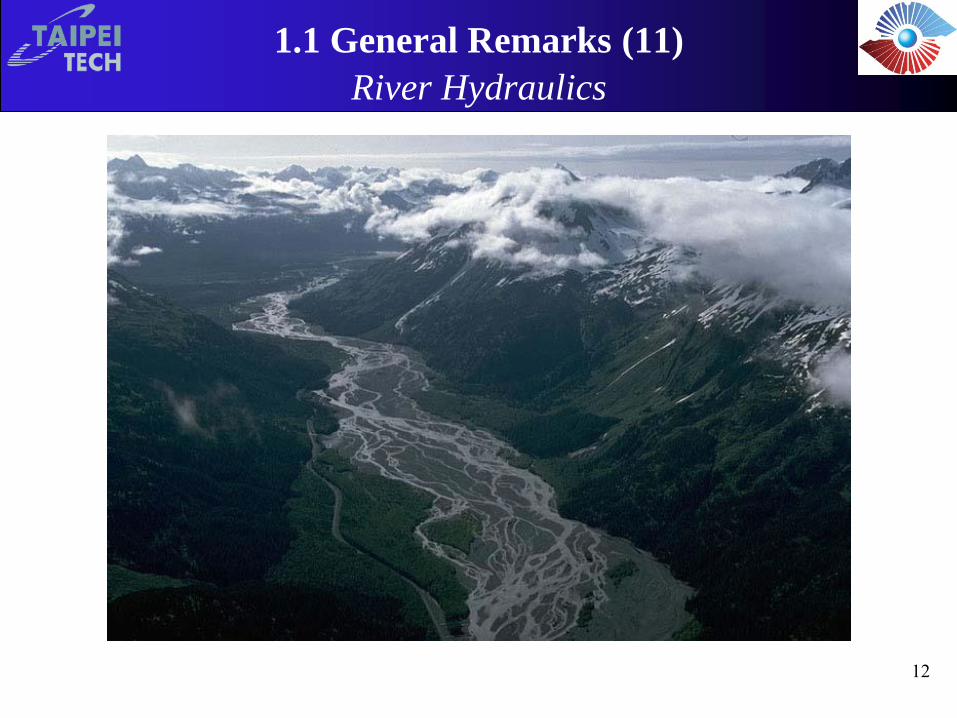
1.1 General Remarks (11) River Hydraulics
12
Applied Computational Fluid Dynamics
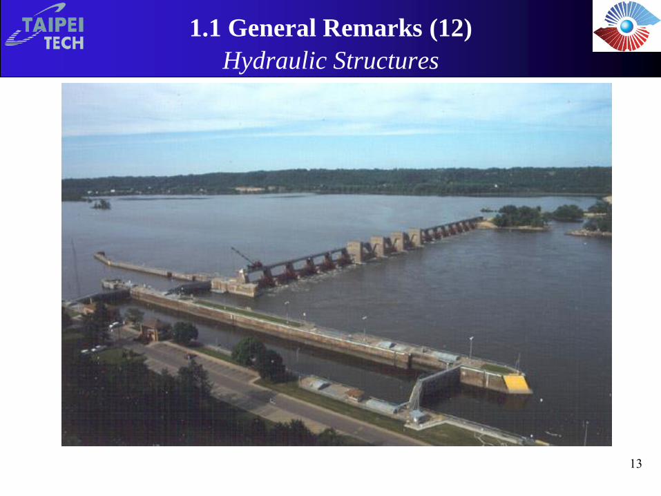
1.1 General Remarks (12) Hydraulic Structures
13
Applied Computational Fluid Dynamics
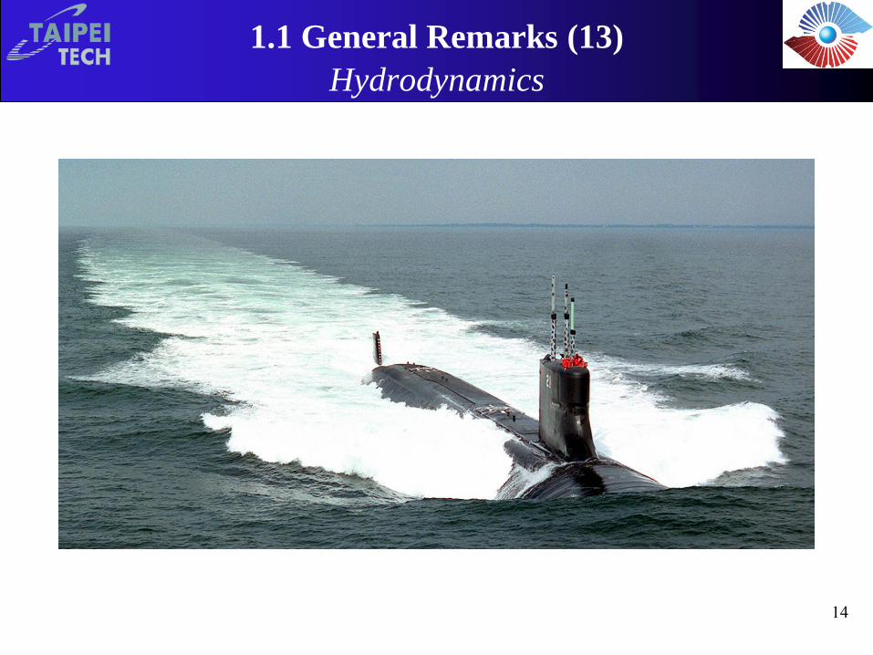
1.1 General Remarks (13) Hydrodynamics
14
Applied Computational Fluid Dynamics
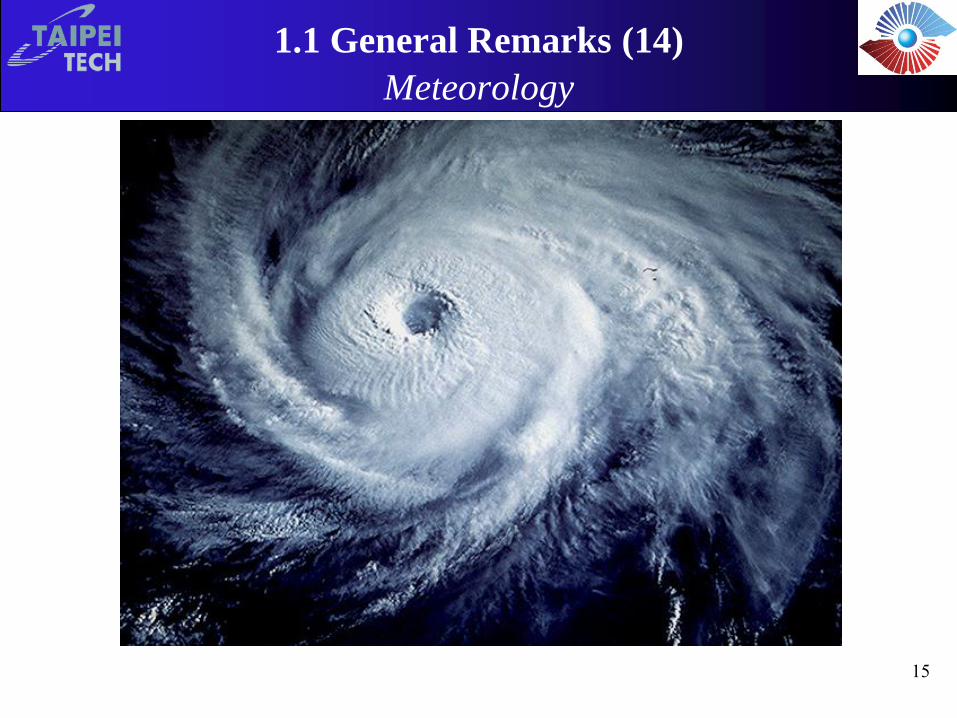
1.1 General Remarks (14) Meteorology
15
Applied Computational Fluid Dynamics
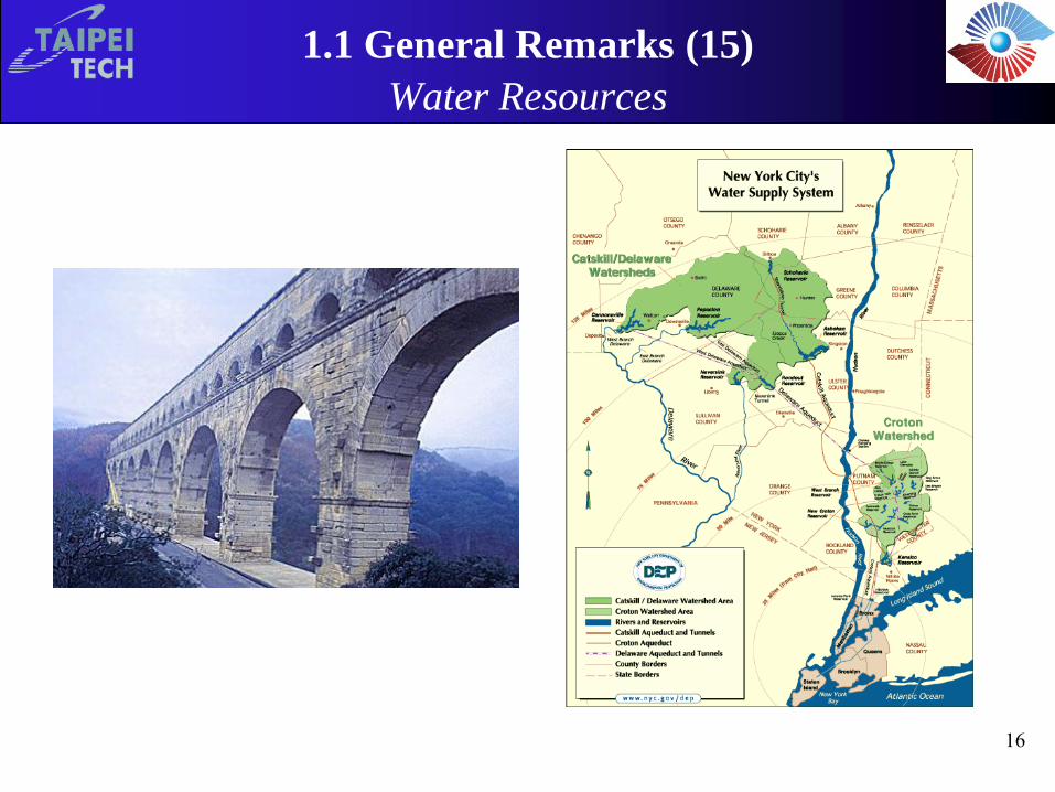
1.1 General Remarks (15) Water Resources
16
Applied Computational Fluid Dynamics
1.2 Methods for Solving Fluid Dynamics Problems (1)
Over the past half century, we have witnessed the rise to importance of a new methodology for attacking the complex problems in fluid mechanics and heat transfer. The new methodology has become known as Computational Fluid Dynamics (CFD).
In this approach, the equations that govern a process of interest are solved numerically. The evolution of numerical methods, especially finite-difference methods for solving ordinary and partial differential equations, started approximately with the beginning of the twentieth century.
The explosion in computational activity did not begin until general availability of high-speed digital computers, occurred in 1960s.
17
Applied Computational Fluid Dynamics
1.2 Methods for Solving Fluid Dynamics Problems (2)
Traditionally, both experimental and theoretical methods have been used to develop designs for equipment and vehicles involving fluid flow and heat transfer. With the advent of the digital computer, a third method, the numerical approach, has become available.
Over the years, computer speed has increased much more rapidly than computer costs. The net effect has been a phenomenal decrease in the cost of performing a given calculation.
The suggestion here is not that computational methods will soon completely replace experimental testing as a means to gather information for design purpose. Rather, it is believed that computer methods will be used even more extensively in the future.
18
Applied Computational Fluid Dynamics
1.2 Methods for Solving Fluid Dynamics Problems (3)
The need for experiments will probably remain for quite some time in applications involving turbulent flow, where it is presently not economically feasible to utilize computational models that are free of empiricism for most practical configurations. This situation is destined to change eventually, since it has become clear that turbulent flows can be solved by direct numerical simulation (DNS) as computer hardware and algorithms improve in the future. The prospects are also bright for the increased use of large-eddy simulations (LES), where modeling is required for only the smallest scales.
In applications involving multiphase flows, boiling, or condensation, especially in complex geometries, the experimental method remains the primary source of design information. Progress is being made in computational models for these flows.
19
Applied Computational Fluid Dynamics
1.2 Methods for Solving Fluid Dynamics Problems (4)
Analytical Fluid Dynamics (AFD)
Mathematical analysis of governing equations,
including exact and approximate solutions.
Computational Fluid Dynamics (CFD)
Numerical solution of the governing equations
Experimental Fluid Dynamics (EFD)
Observation and data acquisition.
20
Applied Computational Fluid Dynamics
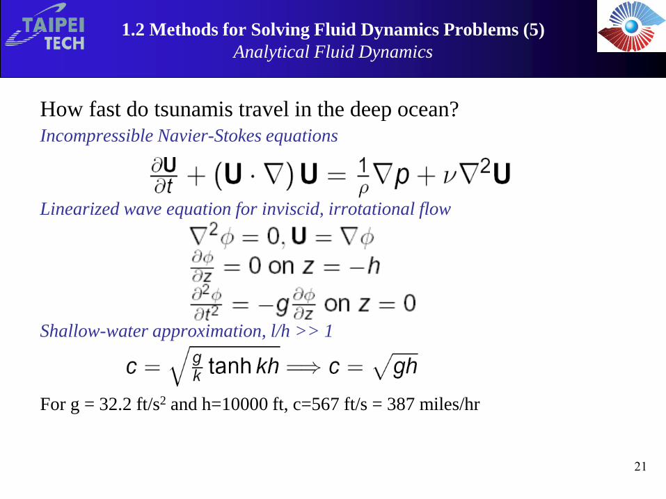
1.2 Methods for Solving Fluid Dynamics Problems (5)
Analytical Fluid Dynamics
How fast do tsunamis travel in the deep ocean?
Incompressible Navier-Stokes equations
Linearized wave equation for inviscid, irrotational flow
Shallow-water approximation, l/h >> 1
For g = 32.2 ft/s2 and h=10000 ft, c=567 ft/s = 387 miles/hr
21
Applied Computational Fluid Dynamics
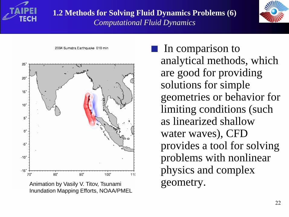
1.2 Methods for Solving Fluid Dynamics Problems (6)
Computational Fluid Dynamics
In comparison to analytical methods, which are good for providing solutions for simple geometries or behavior for limiting conditions (such as linearized shallow water waves), CFD provides a tool for solving problems with nonlinear physics and complex geometry. Animation by Vasily V. Titov, Tsunami
Inundation Mapping Efforts, NOAA/PMEL
22
Applied Computational Fluid Dynamics
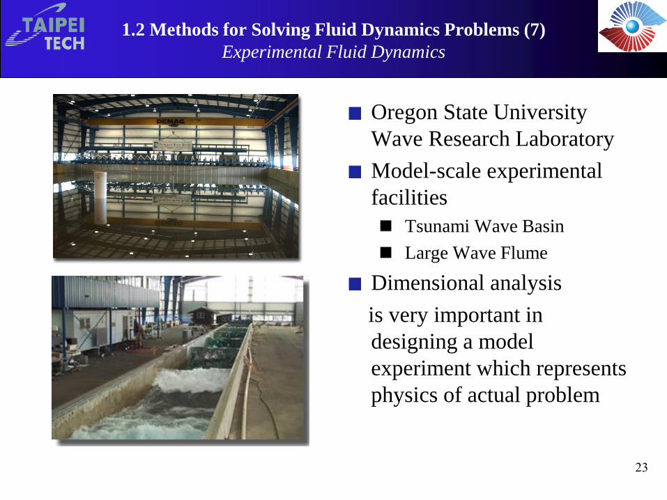
1.2 Methods for Solving Fluid Dynamics Problems (7)
Experimental Fluid Dynamics
Oregon State University
Wave Research Laboratory
Model-scale experimental
facilities
Tsunami Wave Basin
Large Wave Flume
Dimensional analysis
is very important in
designing a model
experiment which represents
physics of actual problem
23
Applied Computational Fluid Dynamics
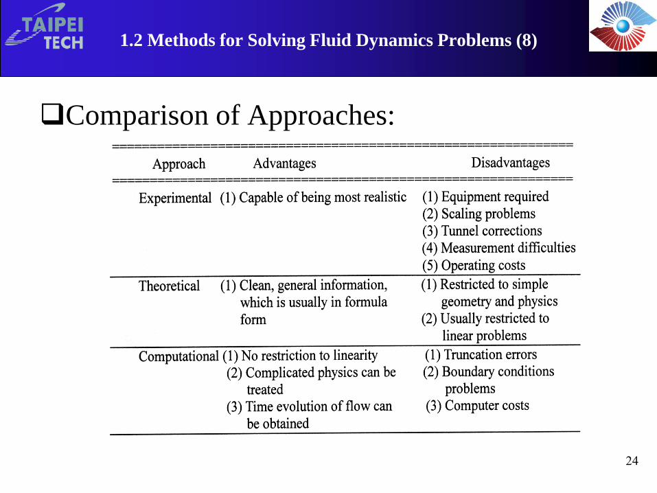
1.2 Methods for Solving Fluid Dynamics Problems (8)
Comparison of Approaches:
24
Applied Computational Fluid Dynamics
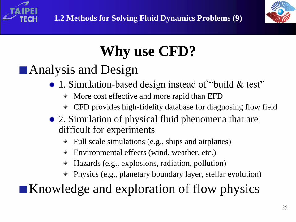
1.2 Methods for Solving Fluid Dynamics Problems (9)
Why use CFD?
Analysis and Design 1. Simulation-based design instead of “build & test”
More cost effective and more rapid than EFD
CFD provides high-fidelity database for diagnosing flow field
2. Simulation of physical fluid phenomena that are difficult for experiments
Full scale simulations (e.g., ships and airplanes)