CONTINUOUS-TIME MARKOV CHAINS by Ward Whitt Department of Industrial Engineering and Operations Research Columbia University New York, NY 10027-6699 Email: [email protected]URL: www.columbia.edu/∼ww2040 December 13, 2012 c Ward Whitt
Transcript
CONTINUOUS-TIME MARKOV CHAINS
by
Ward Whitt
Department of Industrial Engineering and Operations ResearchColumbia University
We now turn to continuous-time Markov chains (CTMC’s), which are a naturalsequel to the study of discrete-time Markov chains (DTMC’s), the Poisson process and theexponential distribution, because CTMC’s combine DTMC’s with the Poisson process andthe exponential distribution. Most properties of CTMC’s follow directly from results aboutDTMC’s, the Poisson process and the exponential distribution. .
Like DTMC’s, CTMC’s are Markov processes that have a discrete state space, which we cantake to be the positive integers. Just as with DTMC’s, we will initially (in §§1-5) focus on thespecial case of a finite state space, but the theory and methods extend to infinite discretestate spaces, provided we impose additional regularity conditions; see §10. We will usuallyassume that the state space is the set {0, 1, 2, . . . , n} containing the first n + 1 nonnegativeintegers for some positive integer n, but any finite set can be so labelled. Just as with DTMC’s,a finite state space allows us to apply square (finite) matrices and elementary linear algebra.The main difference is that we now consider continuous time. We consider a stochasticprocess {X(t) : t ≥ 0}, where time t is understood to be any nonnegative real number. Therandom variable X(t) is the state occupied by the CTMC at time t.
As we will explain in §3, a CTMC can be viewed as a DTMC with altered transition times.Instead of unit times between successive transitions, the times between successive transitionsare allowed to be independent exponential random variables with means that depend only onthe state from which the transition is being made. Alternatively, as we explain in §3.4, aCTMC can be viewed as a DTMC (a different DTMC) in which the transition times occuraccording to a Poisson process. In fact, we already have considered a CTMC with just thisproperty (but infinite state space), because the Poisson process itself is a CTMC. For thatCTMC, the associated DTMC starts in state 0 and has only unit upward transitions, movingfrom state i to state i + 1 with probability 1 for all i. A CTMC generalizes a Poisson processby allowing other transitions. For a Poisson process, X(t) goes to infinity as t→∞. We willbe interested in CTMC’s that have proper limiting distributions as t→∞.
Organization. Here is how the chapter is organized: We start in §2 by discussing transitionprobabilities and the way they can be used to specify the finite-dimensional distributions,which in turn specify the probability law of the CTMC. Then in §3 we describe four differentways to construct a CTMC model, giving concrete examples. In §4 we discuss the specialcase of a birth-and-death process, in which the only possible transitions are up one or downone to a neighboring state. The number of customers in a queue (waiting line) can oftenbe modeled as a birth-and-death process. The special structure of a birth-and-death processmakes the limiting probabilities especially easier to compute. Afterwards, in §5 we indicatehow to calculate the limiting probabilities for a general irreducible CTMC. There are differentways, with the one that is most convenient usually depending on the modeling approach.
The second part is more advanced, focusing on reversibility and stochastic networks. Westart in §6 by introducing reverse-time CTMC’s and reversibility. We apply those notions toa CTMC consisting of several queues in series. in §§7 and 8 we present the basic theory ofopen and closed queueing networks, respectively. in §9 we discuss loss models, starting withthe classical Erlang loss model and then continuing to multi-class multi-facility generalizations:stochastic loss networks.
We conclude with a brief treatment of some more advanced topics. In §10 we discuss theregularity conditions needed for infinite-state CTMC’s. Finally, we discuss four special topicsfor reversible CTMC’s and birth-and-death processes: (i) rates of convergence to steady statecharacterized via the spectral representation of the transition function, (ii) fitting birth-and-
1
death models to data, (iii) stochastic comparisons for birth-and-death processes and (iv) waysto compute first-passage-time distributions in birth-and-death processes. Much more materialis available in the references.
2. Transition Probabilities and Finite-Dimensional Distributions
Just as with discrete time, a continuous-time stochastic process is a Markov process ifthe conditional probability of a future event given the present state and additional informationabout past states depends only on the present state. A CTMC is a continuous-time Markovprocess with a discrete state space, which can be taken to be a subset of the nonnegativeintegers. That is, a stochastic process {X(t) : t ≥ 0} (with an integer state space) is a CTMCif
P (X(s + t) = j|X(s) = i,X(r) = ir, r ∈ As ⊆ [0, s)) = P (X(s + t) = j|X(s) = i) (2.1)
for all states i and j and for all times s > 0 and t > 0. On the left in (2.1), we are conditioningon the values of X(r) for all times r in a subset of “past” times As in addition to the value atthe “present” time s. In general, As could be an arbitrary subset of [0, s) ≡ {r : 0 ≤ r < s},but to have the conditional probability in (2.1) well defined by elementary methods, we assumethat As is a finite subset.
The conditional probabilities P (X(s+t) = j|X(s) = i) are called the transition probabil-ities. We will consider the special case of stationary transition probabilities (sometimesreferred to as homogeneous transition probabilities), occurring when
P (X(s + t) = j|X(s) = i) = P (X(t) = j|X(0) = i) ≡ Pi,j(t) (2.2)
for all states i and j and for all times s > 0 and t > 0; the independence of s characterizes thestationarity. We assume stationary transition probabilities unless stipulated otherwise.
Thus a key concept for CTMC’s is the notion of transition probabilities. However, thetransition probabilities of CTMC’s are not so easy to work with. As a consequence, we usuallydo not directly use transition probabilities when we construct and analyze CTMC models.First, when we construct a CTMC model, we invariably do not directly define the transitionprobabilities (although their structure will be implied by what we do define). Second, afterconstructing a CTMC model, we usually do not calculate the transition probabilities. Instead,we usually calculate the associated limiting probabilities, denoted by αj :
αj ≡ limt→∞
Pi,j(t) ≡ limt→∞
P (X(t) = j|X(0) = i) , (2.3)
because they are much easier to calculate, and because they usually serve as excellent approx-imations for the exact transition probabilities Pi,j(t) when t is large. (We use the notation αfor the limiting probability vector of the CTMC, instead of π, because we reserve π for thelimiting probability vector for an associated DTMC; see §3.1 and Theorem 5.2.)
Consistent with what we have written in (2.3), under regularity conditions, the limitingprobabilities αj will not to depend on the initial state. Indeed, that will be true provided theCTMC is irreducible, which means (just as in discrete time) that it is possible with somepositive probability to get from any state to any other state at some finite time, which mayinvolve multiple transitions. (Just as in discrete time, for irreducibility, we do not requirethat we reach these other states in a single transition.) We assume irreducible CTMC’s unlessstipulated otherwise.
This chapter is largely about constructing CTMC models and calculating the limitingprobability vector α ≡ (α0, α1, . . . , αn). As with DTMC’s, we will also want to apply the
2
limiting probability vector α to answer a variety of related questions of interest. But, torepeat, neither constructing the CTMC model nor calculating the limiting probability vectorα will directly involve the transition probabilities. Nevertheless, the transition probabilitiesare very important for understanding CTMC’s.
Just as in discrete time, the evolution of the transition probabilities over time is describedby the Chapman-Kolmogorov equations, but they take a different form in continuous time. Informula (2.4) below, we consider a sum over all possible states at some intermediate time. Indoing so, we simply write a sum over integers. When we do that, we understand the sum tobe over all possible states.
Lemma 2.1. (Chapman-Kolmogorov equations) For all s ≥ 0 and t ≥ 0,
Pi,j(s + t) =∑
k
Pi,k(s)Pk,j(t) . (2.4)
Proof. We can compute Pi,j(s + t) by considering all possible places the chain could be attime s. We then condition and and uncondition, invoking the Markov property to simplify theconditioning; i.e.,
Using matrix notation, we write P (t) for the square matrix of transition probabilities(Pi,j(t)), and call it the transition function. In matrix notation, the Chapman-Kolmogorovequations reduce to a simple relation among the transition functions involving matrix mul-tiplication:
P (s + t) = P (s)P (t) (2.5)
for all s ≥ 0 and t ≥ 0. It is important to recognize that (2.5) means (2.4). From the perspectiveof abstract algebra, equation (2.5) says that the transition function has a semi-group property,where the single operation is matrix multiplication. (It is not a group because an inverse ismissing.)
A CTMC is well specified if we specify: (1) its initial probability distribution - P (X(0) = i)for all states i - and (2) its transition probabilities - Pi,j(t) for all states i and j and positivetimes t. First, we can use these two elements to compute the distribution of X(t) for each t,namely,
P (X(t) = j) =∑
i
P (X(0) = i)Pi,j(t) . (2.6)
However, in general, we want to do more. We want to know about the joint distributions inorder to capture the dependence structure. Recall that the probability law of a stochas-tic process is understood to be the set of all its finite-dimensional distributions. A finite-dimensional distribution is
for states ji and times ti satisfying 0 ≤ t1 < t2 < · · · < tk. The probability law is specifiedby all these finite-dimensional distributions, considering all positive integers k, and all setsof k states and k ordered times. It is important that we can express any finite-dimensionaldistribution in terms of the initial distribution and the transition probabilities. For example,assuming that t1 > 0, we have
In summary, equation (2.8) shows that we succeed in specifying the full probability lawof the DTMC, as well as all the marginal distributions via (2.6), by speciying the initialprobability distribution - P (X(0) = i) for all i - and the transition probabilities Pi,j(t) for allt, i and j or, equivalently, the transition function P (t). However, when we construct CTMCmodels, as we do next, we do not directly specify the transition probabilities. We will see that,at least in principle, the transition probabilities can be constructed from what we do specify,but we usually do not carry out that step.
3. Modelling
We now turn to modelling: constructing a CTMC model. We saw that a DTMC modelis specified by simply specifying its one-step transition matrix P and the initial probabilitydistribution. Unfortunately, the situation is more complicated in continuous time.
In this section we will describe four different approaches to constructing a CTMC model.With each approach, we will need to specify the initial distribution, so we are focusing onspecifying the model beyond the initial distribution. The four approaches are equivalent: Youget to the same result from each and you can get to each from any of the others. Even thoughthese four approaches are redundant, they are useful because they together give a differentmore comprehensive view of a CTMC. We see different things from different perspectives,much like the Indian fable about the blind men and the elephant, recaptured in the poem byJohn Godfrey Saxe (1816-1887):
The Blind Men and the Elephant
It was six men of IndostanTo learning much inclined,Who went to see the Elephant(Though all of them were blind),That each by observationMight satisfy his mind.
The First approached the Elephant,And happening to fallAgainst his broad and sturdy side,At once began to bawl:“God bless me! but the ElephantIs very like a wall!”
4
The Second, feeling of the tusk,Cried, “Ho! what have we hereSo very round and smooth and sharp?To me tis mighty clearThis wonder of an ElephantIs very like a spear!”
The Third approached the animal,And happening to takeThe squirming trunk within his hands,Thus boldly up and spake:“I see,” quoth he, “the ElephantIs very like a snake!”
The Fourth reached out an eager hand,And felt about the knee.“What most this wondrous beast is likeIs mighty plain,” quoth he;“ Tis clear enough the ElephantIs very like a tree!”
The Fifth, who chanced to touch the ear,Said: “Een the blindest manCan tell what this resembles most;Deny the fact who canThis marvel of an ElephantIs very like a fan!”
The Sixth no sooner had begunAbout the beast to grope,Than, seizing on the swinging tailThat fell within his scope,“I see,” quoth he, “the ElephantIs very like a rope!”
And so these men of IndostanDisputed loud and long,Each in his own opinionExceeding stiff and strong,Though each was partly in the right,And all were in the wrong!
For some applications, one modelling approach may be more natural than the others. Orone modelling approach may be more convenient for analyzing the model.
5
3.1. A DTMC with Exponential Transition Times
In order to construct a CTMC model, it is natural to build on our knowledge of DTMC’s.So we first consider a way to exploit DTMC’s in our construction of the CTMC model. Todo so in the strongest way, we start with a DTMC having a transition matrix P , and thenmodify the way the transitions occur. Instead of having each transition take unit time, nowwe assume that each transition takes a random time. In particular, we assume that the timerequired to make a transition from state i has an exponential distribution with rate νi, andthus mean 1/νi, independent of the history before reaching state i.
This modelling approach is convenient for simulating the CTMC; we can recursively gen-erate successive transitions. This modelling approach also avoids technical complications thatarise in the conventional transition-rate approach, to be introduced in the next subsection.This modelling approach is also appealing because many applications are naturally expressedin this way.
Example 3.1. (Pooh Bear and the Three Honey Trees) A bear of little brain namedPooh is fond of honey. Bees producing honey are located in three trees: tree A, tree B andtree C. Tending to be somewhat forgetful, Pooh goes back and forth among these three honeytrees randomly (in a Markovian manner) as follows: From A, Pooh goes next to B or Cwith probability 1/2 each; from B, Pooh goes next to A with probability 3/4, and to C withprobability 1/4; from C, Pooh always goes next to A. Pooh stays a random time at eachtree. (Assume that the travel times can be ignored.) Pooh stays at each tree an exponentiallength of time, with the mean being 5 hours at tree A or B, but with mean 4 hours at tree C.Construct a CTMC enabling you to find the limiting proportion of time that Pooh spends ateach honey tree.
Note that this problem is formulated directly in terms of the DTMC, describing the randommotion at successive transitions, so it is natural to use this initial modelling approach. Herethe transition matrix for the DTMC is
P =ABC
0 1/2 1/23/4 0 1/41 0 0
.
In the displayed transition matrix P , we have only labelled the rows. The columns are assumedto be labeled in the same order. As specified above, the exponential times spent at the threetrees have means 1/νA = 1/νB = 5 hours and 1/νC = 4 hours.
Given that we have already studied DTMC’s, it is natural to wonder how the steady-stateprobability vector of the CTMC is related to the steady-state probability vector of the DTMC.For the DTMC with transition matrix P (looking at the transition epochs of the CTMC), thesteady state probability vector is π, the unique probability vector satisfying the equation
π = πP . (3.1)
It is significant that, in general, the steady-state probability vector of the CTMCis not π. Thus, we use different notation, referring to the steady-state probability vector ofthe CTMC as α. Fortunately, though, the two steady-state probability vectors turn out to beintimately related. In particular, in §5 we will see that
αj =(πj/νj)
∑
k(πk/νk). (3.2)
6
In §5 we will see how to justify formula (3.2) above and relate it to other ways to calculate thelimiting probabilities for this CTMC. We will then be able to answer the question about thelong-run proportion of time that Pooh spends at each tree.
Finally, when we study renewal theory and semi-Markov processes, we will see that the samesteady-state probability vector α in (3.2) also holds if the random holding times in each state arenot exponentially distributed, provided that they are independent and identically distributed(i.i.d.) with those same means 1/νj . Indeed, this first modelling approach corresponds totreating the CTMC as a special case of a semi-Markov process (SMP). An SMP is a DTMCwith independent random transition times, but it allows the distributions of the intervalsbetween transitions to be non-exponential.
With this initial modelling approach, it is natural to assume, as was the case in Example3.1, that there are no one-step transitions in the DTMC from any state immediately back toitself, but it is not necessary to make that assumption. We get a CTMC from a DTMC andexponential transition times without making that assumption.
However, to help achieve a simple relation between the first two modelling approaches, wemake that assumption here: We assume that there are no one-step transitions fromany state to itself in the DTMC; i.e., we assume that Pi,i = 0 for all i. However, weemphasize that this assumption is not critical, as we will explain after we introduce the thirdmodelling approach. Indeed, we will want to allow transitions from a state immediately to itselfin the fourth - uniformization - modelling approach. That is a crucial part of that modellingapproach.
3.2. Transition Rates and ODE’s
A second modelling approach is based on representing the transition probabilities as thesolution of a system of ordinary differential equations, which allows us to apply well-establishedmodelling techniques from the theory of differential equations in a deterministic setting; e.g.,see Simmons (1991). With this second modelling approach, we directly specify transition rates.
We proceed with that idea in mind, but without assuming knowledge about differentialequations. We focus on the transition probabilities of the CTMC, even though they havenot yet been specified. With the transition probabilities in mind, we assume that there arewell-defined derivatives (from above or from the right) of the transition probabilities at 0. Weassume these derivatives exist, and call them transition rates.
But first we must define zero-time transition probabilities, which we do in the obviousway: We let P (0) = I, where I is the identity matrix; i.e., we set Pi,i(0) = 1 for all i and weset Pi,j(0) = 0 whenever i 6= j. We are just assuming that you cannot go anywhere in zerotime.
We then let the transition rate from state i to state j be defined in terms of the derivatives:
Qi,j ≡ P ′i,j(0+) ≡dPi,j(t)
dt|t=0+ . (3.3)
In (3.3) 0+ appears to denote the right derivative at 0 because Pi,j(t) is not defined for t < 0.This approach is used in most treatments of CTMC’s, but without mentioning derivatives
or right-derivatives. Instead, it is common to assume that
Pi,j(h) = Qi,jh + o(h) as h ↓ 0 if j 6= i (3.4)
andPi,i(h) − 1 = Qi,ih + o(h) as h ↓ 0 , (3.5)
7
where o(h) is understood to be a quantity which is asymptotically negligible as h ↓ 0 afterdividing by h. (Formally, f(h) = o(h) as h ↓ 0 if f(h)/h→ 0 as h ↓ 0.)
For a finite state space, which we have assumed, and for infinite state spaces under extraregularity conditions, we will have
−Qi,i ≡∑
j,j 6=i
Qi,j (3.6)
because the transition probabilities Pi,j(t) sum over j to 1. Moreover, we have
−Qi,i = νi for all i , (3.7)
because we have assumed that Pi,i = 0 in the first modelling approach.In other words, these two assumptions mean that
limh↓0
Pi,j(h)− Pi,j(0)
h= Qi,j for all i and j , (3.8)
which is just what is meant by (3.3).In summary, we first assumed that transition probabilities are well defined, at least for zero
time and small positive time intervals, and then assume that they are differentiable from theright at 0. We remark that it is possible to weaken that assumption, and only assume that thetransition probabilities are continuous at 0: P (h) → P (0) ≡ I as h ↓ 0. Then it is possible toprove that the derivatives exist; see §§II.1 and II.2 of Chung (1967).
Having defined the transition rates in terms of the assumed behavior of the transitionprobabilities in a very short (asymptotically negligible) interval of time, we can specify theCTMC model by specifying these transition rates; i.e., we specify the transition-rate matrix Q,having elements Qi,j. (But we do not first fully define the transition probabilities themselves!)Thus, just as we specify a DTMC model via a matrix P , we can specify a CTMC model viathe transition-rate matrix Q.
When specifying the transition-rate matrix Q, it suffices to specify the off-diagonal elementsQi,j for i 6= j, because the diagonal elements Qi,i are always defined by (3.6). The off-diagonalelements are always nonnegative, whereas the diagonal elements are always negative. Eachrow sum of Q is zero.
Even though this modelling approach for CTMC’s is similar to what we did for DTMC’s,it is more complicated, because the rate matrix Q is harder to interpret than the one-steptransition matrix P . (The discussion above is intended to help interpretation.) In fact, thisapproach to CTMC modelling is perhaps best related to modelling with ordinary differentialequations, as mentioned at the beginning of this subsection.
To construct the transition probabilities Pi,j(t) from the transition rates Qi,j ≡ P ′i,j(0+), weapply the Chapman-Kolmogorov equations in Lemma 2.1 in order to show that the transitionprobabilities satisfy two systems of ordinary differential equations (ODE’s) generatedby the transition rates. In matrix notation, these will be simple first-order linear ODE’s.
Theorem 3.1. (Kolmogorov forward and backward ODE’s) The transition probabilitiessatisfy both the Kolmogorov forward differential equations
P ′i,j(t) =∑
k
Pi,k(t)Qk,j for all i and j , (3.9)
which in matrix notation is the matrix ODE
P ′(t) = P (t)Q , (3.10)
8
and the Kolmogorov backward differential equations
P ′i,j(t) =∑
k
Qi,kPk,j(t) for all i and j , (3.11)
which in matrix notation is the matrix ODE
P ′(t) = QP (t) , (3.12)
Proof. We start with the forward equation, using matrix notation. We apply the Chapman-Kolmogorov equations in Lemma 2.1 to write
P (t + h) = P (t)P (h) ,
and then do an asymptotic analysis as h ↓ 0. (This is tantamount to doing a careful asymptoticanalysis of what happens in a small interval after time t.) We subtract P (t) from both sidesand divide by h, to get
P (t + h)− P (t)
h= P (t)
P (h) − I
h,
where I is the identity matrix. Recalling that I = P (0), we can let h ↓ 0 to get the desiredresult (3.10). To get the backward equation (3.12), we start with
P (t + h) = P (h)P (t)
and reason in the same way. (This is tantamount to doing a careful asymptotic analysis ofwhat happens in a small interval after time 0, and then applying P (t) thereafter.)
To help remember which ODE is forward and which is backwards, note that P (t)Qappearing on the righthand side of the forward ODE is in alphabetic order, whereas QP (t)appearing on the righthand side of the backward ODE is in reverse (backward) alphabeticorder.
With a finite state space, both ODE’s are always well defined. With an infinite state space,there can be technical problems, because there could be infinitely many transitions in finitetime; see §10. With an infinite state space, the forward ODE can be more problematic, becauseit presumes the process got to time t before doing the asymptotic analysis. Here we assumea finite state space, so we do not encounter those pathologies. Under regularity conditions,those pathologies will not occur with infinite state spaces either.
To obtain the transition function P (t) from the transition-rate matrix Q, we can solve oneof these ODE’s. In preparation, we review the simple one-dimensional story. Suppose that wehave an ODE f ′(t) = cf(t), where f is understood to be a differentiable real-valued functionf with known initial value f(0). If we divide both sides by f(t), we get f ′(t)/f(t) = c. Sincef ′(t)/f(t) is the derivative of log f(t), we can integrate to get
log f(t)− log f(0) = ct or f(t) = f(0)ect, t ≥ 0 .
Thus we see that f must be an exponential function.Closely paralleling the real-valued case, the matrix ODE’s in (3.10) and (3.12) have an
exponential solution, but now a matrix-exponential solution. (Since P (0) = I, the initialcondition plays no role, just as above when f(0) = 1.) In particular, as a consequence ofTheorem 3.1, we have the following corollary.
9
Theorem 3.2. (matrix exponential representation) The transition function can be ex-pressed as a matrix-exponential function of the rate matrix Q, i.e.,
P (t) = eQt ≡∞∑
n=0
Qntn
n!(3.13)
This matrix exponential is the unique solution to the two ODE’s with initial condition P (0) = I.
Proof. If we verify or assume that we can interchange summation and differentiation in(3.13), we can check that the displayed matrix exponential satisfies the two ODE’s:
d
dt
∞∑
n=0
Qntn
n!=
∞∑
n=0
d
dt
Qntn
n!=
∞∑
n=0
nQntn−1
n!= Q
∞∑
n=0
Qntn
n!= QeQt .
We give a full demonstration at the end of §3.4.However, in general the transition function P (t) is not elementary to compute via (3.13);
see Moler and Van Loan (2003). Indeed, one of the ways to evaluate the matrix-exponentialfunction displayed in (3.13) is to numerically solve one of the ODE’s as expressed in (3.10) or(3.12).
We now illustrate this second modelling approach with an example.
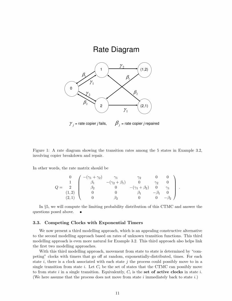
Example 3.2. (Copier Breakdown and Repair) Consider two copier machines that aremaintained by a single repairman. Machine i functions for an exponentially distributed amountof time with mean 1/γi, and thus rate γi, before it breaks down. The repair times for copieri are exponential with mean 1/βi, and thus rate βi, but the repairman can only work on onemachine at a time. Assume that the machines are repaired in the order in which they fail.Suppose that we wish to construct a CTMC model of this system, with the goal of finding thelong-run proportions of time that each copier is working and the repairman is busy. How canwe proceed?
An initial question is: What should be the state space? Can we use 4 states, letting thestates correspond to the subsets of failed copiers? Unfortunately, the answer is “no,” becausein order to have the Markov property we need to know which copier failed first when bothcopiers are down. However, we can use 5 states with the states being: 0 for no copiers failed, 1for copier 1 is failed (and copier 2 is working), 2 for copier 2 is failed (and copier 1 is working),(1, 2) for both copiers down (failed) with copier 1 having failed first and being repaired, and(2, 1) for both copiers down with copier 2 having failed first and being repaired. (Of course,these states could be relabelled 0, 1, 2, 3 and 4, but we do not do that.)
From the problem specification, it is natural to work with transition rates, where thesetransition rates are obtained directly from the originally-specified failure rates and repair rates(the rates of the exponential random variables). In Figure 1 we display a rate diagramshowing the possible transitions with these 5 states together with the appropriate rates. It canbe helpful to construct such rate diagrams as part of the modelling process.
From Figure 1, we see that there are 8 possible transitions. The 8 possible transitionsshould clearly have transition rates
In §5, we will compute the limiting probability distribution of this CTMC and answer thequestions posed above.
3.3. Competing Clocks with Exponential Timers
We now present a third modelling approach, which is an appealing constructive alternativeto the second modelling approach based on rates of unknown transition functions. This thirdmodelling approach is even more natural for Example 3.2. This third approach also helps linkthe first two modelling approaches.
With this third modelling approach, movement from state to state is determined by “com-peting” clocks with timers that go off at random, exponentially-distributed, times. For eachstate i, there is a clock associated with each state j the process could possibly move to in asingle transition from state i. Let Ci be the set of states that the CTMC can possibly moveto from state i in a single transition. Equivalently, Ci is the set of active clocks in state i.(We here assume that the process does not move from state i immediately back to state i.)
11
Each time the CTMC moves to state i, clocks with timers are set or reset, if necessaryto go off at random times Ti,j for each j ∈ Ci. Each clock has an exponential timer; i.e., therandom time Ti,j is given an exponential distribution with (positive finite) rate Qi,j and thusmean 1/Qi,j (depending on i and j). Moreover, we assume that these newly set times Ti,j aremutually independent and independent of the history of the CTMC prior to that transitiontime. By the lack-of-memory property of the exponential distribution, resetting running timersis equivalent (leaves the probability law of the stochastic process unchanged) to not resettingthe times, and letting the timers continue to run.
Example 3.3. (Copier Breakdown and Repair Revisited) At this point we should re-consider Example 3.2 and observe that it is even more natural to define the CTMC throughthe proposed clocks with random timers. The random times triggering transitions are theexponential times to failure and times to repair specified in the original problem formulation.However, there is a difference: In the actual system, those random times do not get reset ateach transition epoch. But, because of the lack-of-memory property of the exponential dis-tribution, a timer that is still going can be reset at any time, including one of these randomtransition times, without changing the distribution of the remaining time. Thus the clockswith random timers does produce a valid representation of the desired CTMC model.
We now discuss the implications of the model specification in terms of exponential timers.As a consequence of these probabilistic assumptions, with probability 1, no two timers evergo off at the same time. (Since the exponential distribution is a continuous distribution, theprobability of any single possible value is 0.) Let Ti be the time that the first timer goes off instate i and let Ni be the index j of the random timer that the first goes off; i.e.,
Ti ≡ minj{Ti,j} (3.14)
andNi ≡ j such that Ti,j = Ti . (3.15)
(The index j yielding the minimum is often called the argmin.) We then let the let the processmove from state i next to state Ni after an elapsed time of Ti, and we repeat the process,starting from the new state Ni.
To understand the implications of these exponential clocks, recall basic properties of theexponential distribution. Recall that the minimum of several independent exponentialrandom variables is again an exponential random variable with a rate equal to the sum ofthe rates. Hence, Ti has an exponential distribution, i.e.,
P (Ti ≤ t) = 1− e−νit, t ≥ 0 , (3.16)
whereνi ≡ −Qi,i =
∑
j,j 6=i
Qi,j , (3.17)
as in (3.6) and (3.7). (Again we use the assumption that Pi,i = 0 in the first modellingapproach.)
Next, recall that, when considering several independent exponential random variables, eachexponential random variable is the exponential random variable yielding the minimumwith a probability proportional to its rate, so that
P (Ni = j) =Qi,j
∑
k,k 6=i Qi,k=
Qi,j
νifor j 6= i . (3.18)
12
Finally, as discussed before in relation to the exponential distribution, the random variablesTi and Ni are independent random variables:
P (Ti ≤ t,Ni = j) = P (Ti ≤ t)P (Ni = j) = (1− e−νit)
(
Qi,j
νi
)
for all t and j .
After each transition, new timers are set, with the distribution of Ti,j being the same ateach transition to state i. So new timer values are set only at transition epochs. However, bythe lack-of-memory property of the exponential distribution, the distribution of the remainingtimes Ti,j and the associated random variables Ti and Ni would be the same any time welooked at the process in state i.
The analysis we have just done translates this clock formulation directly into a DTMCwith exponential transition times, as in our first modelling approach in §3.1: The one-steptransition matrix P of the DTMC is
Pi,j = P (Ni = j) =Qi,j
∑
k,k 6=i Qi,k=
Qi,j
νifor j 6= i , (3.19)
with Pi,i = 0 for all i, as specified in (3.18), while the rate νi of the exponential holding timein state i is specified in (3.17).
Moreover, it is easy to see how to define transition rates as required for the second modellingapproach. We just let Qi,j be the rate of the exponential timer Ti,j. We have chosen thenotation to make these associations obvious. Moreover, we can use the exponential timersto prove that the transition probabilities of the CTMC are well defined and do indeed havederivatives at the origin.
The construction here makes it clear how to relate the first two modelling approaches.Given the rate matrix Q, we define the one-step transition matrix P of the DTMC by (3.19)and the rate νi of the exponential transition time in state i by (3.17). That procedure gives usan underlying DTMC P with Pi,i = 0 for all i.
These equations also tell us how to go the other way: Given (P, ν), we let
Qi,j = νiPi,j for j 6= i and Qi,i = −∑
j,j 6=i
Qi,j = νi for all i . (3.20)
From this analysis, we see that the CTMC is uniquely specified by the rate matrix Q; i.e.,two different Q matrices produce two different CTMC’s (two different probability laws, i.e.,two different f.d.d.’s). That property also holds for the first modelling approach, provided thatwe assume that Pi,i = 0 for all i. Otherwise, the same CTMC can be represented by differentpairs (P, ν). There is only one if we require, as we have done, that there be no transitions fromany state immediately back to itself.
We can also use this third modelling approach to show that the probability law of the CTMCis unaltered if there are initially one-step transitions from any state to itself. If we are initiallygiven one-step transitions from any state to itself, we can start by removing them, but withoutaltering the probability law of the original CTMC. If we remove a DTMC transition from statei to itself, we must compensate by increasing the transition probabilities to other states andincreasing the mean holding time in state i. To do so, we first replace initial transition matrixP with transition matrix P , where Pi,i = 0 for all i. To do so without altering the CTMC, wemust let the new transition probability be the old conditional probability given that there isno transition from state i to itself; i.e., we let
Pi,j =Pi,j
1− Pi,ifor all i and j . (3.21)
13
We never divide by zero, because Pi,i < 1 (assuming that the chain has more than two statesand is irreducible). Since we have eliminated DTMC transitions from state i to itself, we mustmake the mean transition time larger to compensate. In particular, we replace 1/νi by 1/νi,where
1/νi =(1/νi)
1− Pi,ior νi = νi(1− Pi,i) . (3.22)
Theorem 3.3. (removing transitions from a state back to itself) The probability lawof the CTMC is unaltered by removing one-step transitions from each state to itself, accordingto (3.21) and (3.22).
Proof. The tricky part is recognizing what needs to be shown. Since (1) the transitionrates determine the transition probabilities, as shown in §3.2, (2) the transition probabilitiesdetermine the finite-dimensional distributions and (3) the finite-dimensional distributions areregarded as the probability law of the CTMC, as shown in §2, it suffices to show that we havethe right transition rates. So that is what we show.
Applying (3.20), we see that the transition rates of the new CTMC (denoted by a hat) are
Qi,j ≡ νiPi,j = νi(1− Pi,i)Pi,j
(1− Pi,i)= νiPi,j , (3.23)
just as in (3.20).In closing, we remark that this third modelling approach with independent clocks corre-
sponds to treating the CTMC as a special case of a generalized semi-Markov process(GSMP); e.g., see Glynn (1989). For general GSMP’s, the clocks can run at different speedsand the timers can have nonexponential distributions.
3.4. Uniformization: A DTMC with Poisson Transitions
Our final modelling approach is not really a direct modelling approach, but rather anintermediate modelling approach, starting from the first modelling approach involving a DTMCwith exponential transition times, that facilitates further analysis. Indeed, this modellingapproach can be regarded as a special case of the first modelling approach. But it provides adifferent view of a CTMC.
In our first modelling approach, involving a DTMC with exponential transition times, themeans of those transition times 1/νi could vary from state to state. However, if it happenedthat these means were all the same, then we could represent the CTMC directly as a DTMCwith transitions governed by an independent Poisson process, because in a Poisson process thetimes between transitions are IID exponential random variables.
Specifically, if the mean transition time is 1/ν0 for all states, then we can generate alltransitions from a Poisson process with rate ν0. Let {Yn : n ≥ 0} be the DTMC with one-steptransition matrix P and let {N(t) : t ≥ 0} be an independent Poisson process with rate ν0.Under that condition, the CTMC {X(t) : t ≥ 0} can be constructed as a random timechange of the DTMC {Yn : n ≥ 0} by the Poisson process {N(t) : t ≥ 0}, i.e.,
X(t) = YN(t), t ≥ 0 . (3.24)
As a consequence,
Pi,j(t) ≡ P (X(t) = j|X(0) = i) =
∞∑
k=0
P ki,jP (N(t) = k) =
∞∑
k=0
P ki,j
e−ν0t(ν0t)k
k!. (3.25)
14
This situation may appear to be very special, but actually any finite-state CTMC canbe represented in this way. We can achieve this representation by using the technique ofuniformization, which means making the rates uniform or constant.
We make the rates uniform without changing the probability law of the CTMC by intro-ducing one-step transitions from some states to themselves, which we can regard as fictitioustransitions, because the process never actually moves. We can generate potential transi-tions from a Poisson process with rate λ, where λ is chosen so that
νi ≡ −Qi,i =∑
j,j 6=i
Qi,j ≤ λ for all i , (3.26)
as in (3.17).When the CTMC is in state i, each of these potential transitions is a real transition (to
another state) with probability νi/λ, while the potential transition is a fictitious transition (atransition from state i back to state i, meaning that we remain in state i at that time) withprobability 1−(νi/λ), independently of past events. In other words, in each state i, we performindependent thinning of the Poisson process having rate λ, creating real transitions instate i according to a Poisson process having rate νi, just as in the original model.
The uniformization construction requires that we change the transition matrix of the em-bedded DTMC. The new one-step transition matrix allows transitions from a state to itself.In particular, the new one-step transition matrix P is constructed from the CTMC transitionrate matrix Q and λ satisfying (3.26) by letting
Pi,j =Qi,j
λfor j 6= i (3.27)
and
Pi,i = 1−∑
j,j 6=i
Pi,j = 1−νi
λ= 1 +
Qi,i
λ= 1−
∑
j,j 6=i Qi,j
λ. (3.28)
In matrix notation,P = I + λ−1Q . (3.29)
Note that we have done the construction to ensure that P is a bonafide Markov chain transitionmatrix; it is nonnegative with row sums 1.
Uniformization is useful because it allows us to apply properties of DTMC’s to analyzeCTMC’s. For the general CTMC characterized by the rate matrix Q, we have transitionprobabilities Pi,j(t) expressed via P in (3.27)-(3.29) and λ as
Pi,j(t) ≡ P (X(t) = j|X(0) = i) =∞∑
k=0
P ki,jP (N(t) = k) =
∞∑
k=0
P ki,j
e−λt(λt)k
k!, (3.30)
where P is the DTMC transition matrix constructed in (3.27)-(3.29). We also have represen-tation (3.24) provided that the DTMC {Yn : n ≥ 0} is governed by the one-step transitionmatrix P and the Poisson process {N(t) : t ≥ 0} has rate λ in (3.26).
But how do we know that equations (3.27) and (3.30) are really correct?
Theorem 3.4. (validity of uniformization) The CTMC constructed via (3.27) and (3.30)leaves the probability law of the CTMC unchanged.
15
Proof. We can justify the construction by showing that the transition rates are the same.Starting from (3.30), we see that, for i 6= j,
Pi,j(h) =∑
k
P ki,j
e−λh(λh)k
k!
= λhe−λhP 1i,j + o(h) = λhe−λh Qi,j
λ+ o(h) = Qi,jh + o(h) as h ↓ 0 , (3.31)
consistent with (3.4), while
Pi,i(h)− 1 =∑
k
P ki,i
e−λh(λh)k
k!− 1
= P 0i,ie−λh + λhe−λhP 1
i,i + o(h) − 1
= (1− λh + o(h)) + (λh + o(h))
(
1 +Qi,i
λ
)
+ o(h)− 1
= Qi,ih + o(h) as h ↓ 0 , (3.32)
consistent with (3.5).We now give a full proof of Theorem 3.2, showing that the transition function P (t) can be
expressed as the matrix exponential eQt.
Proof of Theorem 3.2. (matrix-exponential representation) Apply (3.27) to see thatP = λ−1Q + I. Then substitute for P in (3.30) to get
P (t) =
∞∑
k=0
P k e−λt(λt)k
k!=
∞∑
k=0
(λ−1Q + I)ke−λt(λt)k
k!= e−λt
∞∑
k=0
(Q + λI)ktk
k!
= e−λte(Q+λI)t = e−λteQteλt = eQt ≡
∞∑
k=0
Qktk
k!.
In §5 we will show how uniformization can be applied to quickly determine existence,uniqueness and the form of the limiting distribution of a CTMC. Now we consider a specialclass of CTMC’s that both often arise and are easy to analyze.
4. Birth-and-Death Processes
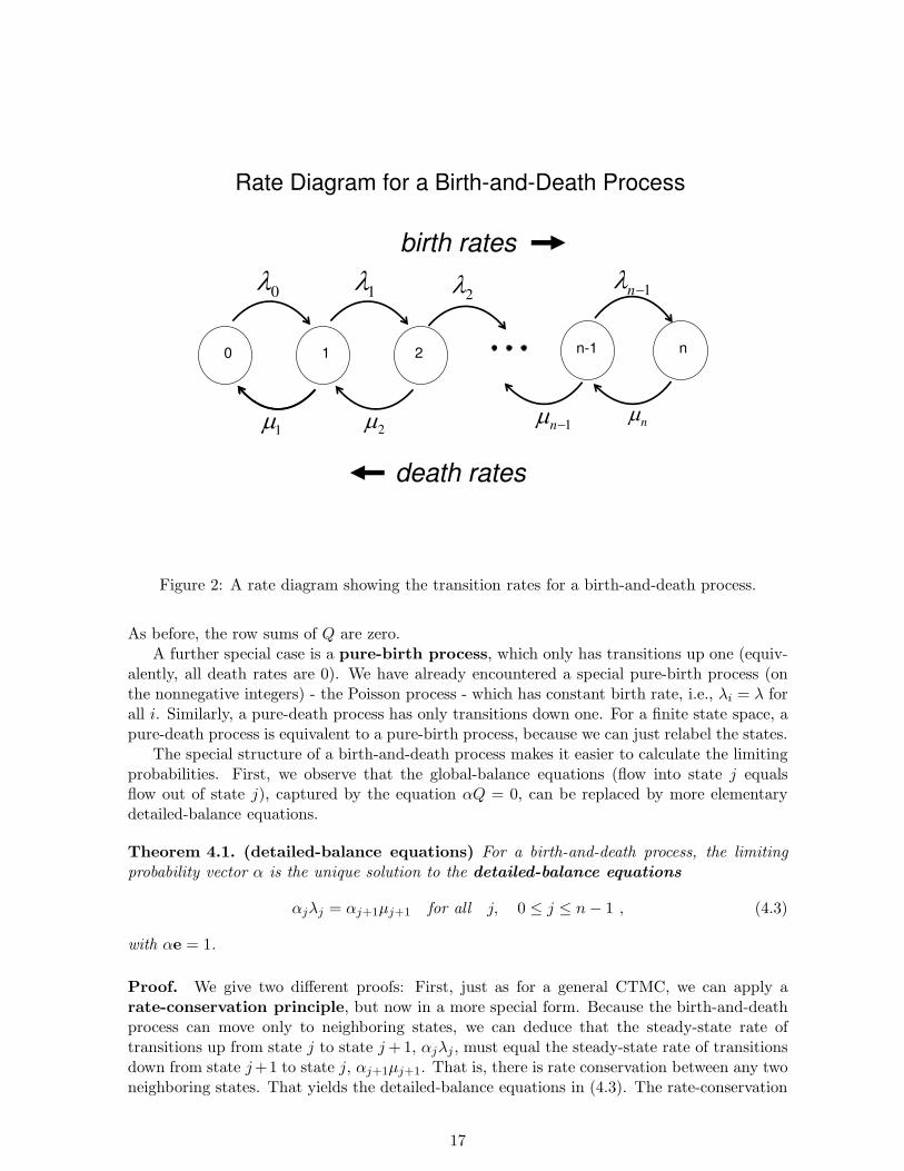
Many CTMC’s have transitions that only go to neighboring states, i.e., either up oneor down one; they are called birth-and-death processes. Motivated by population models, atransition up one is called a birth, while a transition down one is called a death. The birthrate in state i is denoted by λi, while the death rate in state i is denoted by µi. The ratediagram for a birth-and-death process (with state space {0, 1, . . . , n}) takes the simple linearform shown in Figure 2.
Thus, for a birth-and-death process, the CTMC transition rates take the special form
Qi,i+1 = λi, Qi,i−1 = µi and Qi,j = 0 if j /∈ {i− 1, i, i + 1}, 1 ≤ i ≤ n− 1 , (4.1)
with
Q0,1 = λ0, Q0,j = 0 if j /∈ {0, 1}, Qn,n−1 = µn and Qn,j = 0 if j /∈ {n− 1, n} .(4.2)
16
Rate Diagram for a Birth-and-Death Process
birth rates
0
1n21
1
0
2 1n
nn-121
n
death rates
Figure 2: A rate diagram showing the transition rates for a birth-and-death process.
As before, the row sums of Q are zero.A further special case is a pure-birth process, which only has transitions up one (equiv-
alently, all death rates are 0). We have already encountered a special pure-birth process (onthe nonnegative integers) - the Poisson process - which has constant birth rate, i.e., λi = λ forall i. Similarly, a pure-death process has only transitions down one. For a finite state space, apure-death process is equivalent to a pure-birth process, because we can just relabel the states.
The special structure of a birth-and-death process makes it easier to calculate the limitingprobabilities. First, we observe that the global-balance equations (flow into state j equalsflow out of state j), captured by the equation αQ = 0, can be replaced by more elementarydetailed-balance equations.
Theorem 4.1. (detailed-balance equations) For a birth-and-death process, the limitingprobability vector α is the unique solution to the detailed-balance equations
αjλj = αj+1µj+1 for all j, 0 ≤ j ≤ n− 1 , (4.3)
with αe = 1.
Proof. We give two different proofs: First, just as for a general CTMC, we can apply arate-conservation principle, but now in a more special form. Because the birth-and-deathprocess can move only to neighboring states, we can deduce that the steady-state rate oftransitions up from state j to state j + 1, αjλj , must equal the steady-state rate of transitionsdown from state j +1 to state j, αj+1µj+1. That is, there is rate conservation between any twoneighboring states. That yields the detailed-balance equations in (4.3). The rate-conservation
17
principle itself follows from a simple observation. In the time interval [0, t], the number oftransitions up from state j to state j + 1 can differ by at most by one from the number oftransitions down from state j + 1 to state j.
From the perspective of a general CTMC, we already have established that α is theunique solution to αQ = 0 with αe = 1. For a birth-and-death process, the jth equation in thesystem αQ = 0 is
From (4.3)-(4.5), we see that the sum of the first j equations of the form (4.4) and (4.5) fromαQ = 0 coincides with the jth detailed-balance equation in (4.3), while the difference betweenthe jth and (j− 1)st detailed-balance equations coincides with the jth equation from (4.4) and(4.5). Hence the two characterizations are equivalent.
In fact, it is not necessary to solve a system of linear equations each time we want tocalculate the limiting probability vector α, because we can analytically solve the detailed-balance equations to produce an explicit formula.
Theorem 4.2. (limiting probabilities) For a birth-and-death process with state space {0, 1, . . . , n},
αj =rj
∑nk=0 rk
0 ≤ j ≤ n , (4.6)
where
r0 = 1 and rj =λ0 × λ1 × · · · × λj−1
µ1 × µ2 × · · · × µj. (4.7)
Proof and Discussion. By virtue of Theorem 4.1, it suffices to solve the detailed-balanceequations in (4.3). We can do that recursively:
αj =λj−1
µjαj−1 for all j ≥ 1 ,
which implies thatαj = rjα0 for all j ≥ 1 ,
for rj in (4.7). We obtain the final form (4.6) when we require that αe = 1.
Example 4.1. (a small barbershop) Consider a small barbershop, where there are onlytwo barbers, each with his own barber chair. Suppose that there is only room for at most 5customers, with 2 in service and 3 waiting. Assume that potential customers arrive accordingto a Poisson process at rate λ = 6 per hour. Customers arriving when the system is fullare blocked and lost, leaving without receiving service and without affecting future arrivals.Assume that the duration of each haircut is an independent exponential random variable witha mean of µ−1 = 15 minutes. Customers are served in a first-come first-served manner by thefirst available barber.
We can ask a variety of questions: (a) What is the long-run proportion of time there aretwo customers in service plus two customers waiting? (b) What is the (long-run) proportionof time each barber is busy? We might then go on to ask how this long-run behavior wouldchange if we changed the number of barbers or the number of waiting spaces.
18
We start by constructing the model. Let Q(t) denote the number of customers in thesystem at time t. Then the stochastic process {Q(t) : t ≥ 0} is a birth-and-death process withsix states: 0, 1, 2, 3, 4, 5. Indeed, this is a standard queueing model, commonly referred toas the M/M/2/3 queue. The first M means a Poisson arrival process (M for Markov), thesecond M means IID exponential service times (M again for Markov), the 2 is for 2 servers,and the 3 is for 3 additional waiting spaces.) It is common to use λ to denote the arrival rateand µ the service rate of each server.
We can represent the CTMC in terms of competing exponential timers, as in §3.3. Thepossible triggering events are an arrival (birth), causing the state to go up 1, or a departure(death), causing the state to go down 1. It is of course important that these are independentexponential random variables.
The blocking alters the arrival process. The blocking means that no arrivals can enter instate 5. By making the state space {0, 1, . . . , 5}, we have accounted for the blocking. Since theinterarrival times of a Poisson process have an exponential distribution, there are active clockswith exponential timers corresponding to the event of a new arrival in states 0-4. The arrivalclock in state i has mean 1/λi = 1/λ, where λ = 6 per hour is the arrival rate of the Poissonprocess. Hence the birth rates are λi = 6, 0 ≤ i ≤ 4. We have λ5 = 0, because there are noarrivals when the system is full.
Since the service times are independent exponential random variables, the active clockscorresponding to departures also can be represented as exponential random variables. (Recallthat the minimum of independent exponential variables is again exponential with a rate equalto the sum of the rates.) There are active clocks with exponential timers corresponding to theevent of a new departure in states 1-5. The departure clock in state i has mean 1/µi, whereµi is the death rate to be determined. Since the mean service time is 1/µ = 15 minutes, theservice rate for each barber is µ = 1/15 per minute or µ = 4 per hour. However, we mustremember that the service rate applies to each server separately. Since we are measuring timein hours, the death rates are µ1 = µ = 4, µ2 = µ3 = µ4 = µ5 = 2µ = 8. We have µ0 = 0 sincethere can be no departures from an empty system.
Given the birth rates and death rates just defined, we can draw the rate diagram for thesix states 0, 1, . . . , 5, as in Figure 2. The associated rate matrix is now
We now can apply Theorem 4.2 to calculate the limiting probabilities. From (4.6) and(4.7),
αj =rj
r0 + r1 + · · · r5, 0 ≤ j ≤ 5 ,
where r0 = 1 and
rj =λ0 × λ1 × · · · × λj−1
µ1 × µ2 × · · · × µj, 1 ≤ j ≤ 5 .
Here
r0 = 1 =512
512
r1 =6
4=
3
2=
768
512
19
r2 =6× 6
4× 8=
36
32=
9
8=
576
512
r3 =6× 6× 6
4× 8× 8=
27
32=
432
512
r4 =27× 6
32× 8=
81
128=
324
512
r5 =81× 6
128× 8=
243
512
Hence,
α0 =512
2855, α1 =
768
2855, α2 =
576
2855, α3 =
432
2855,
α4 =324
2855and α5 =
243
2855.
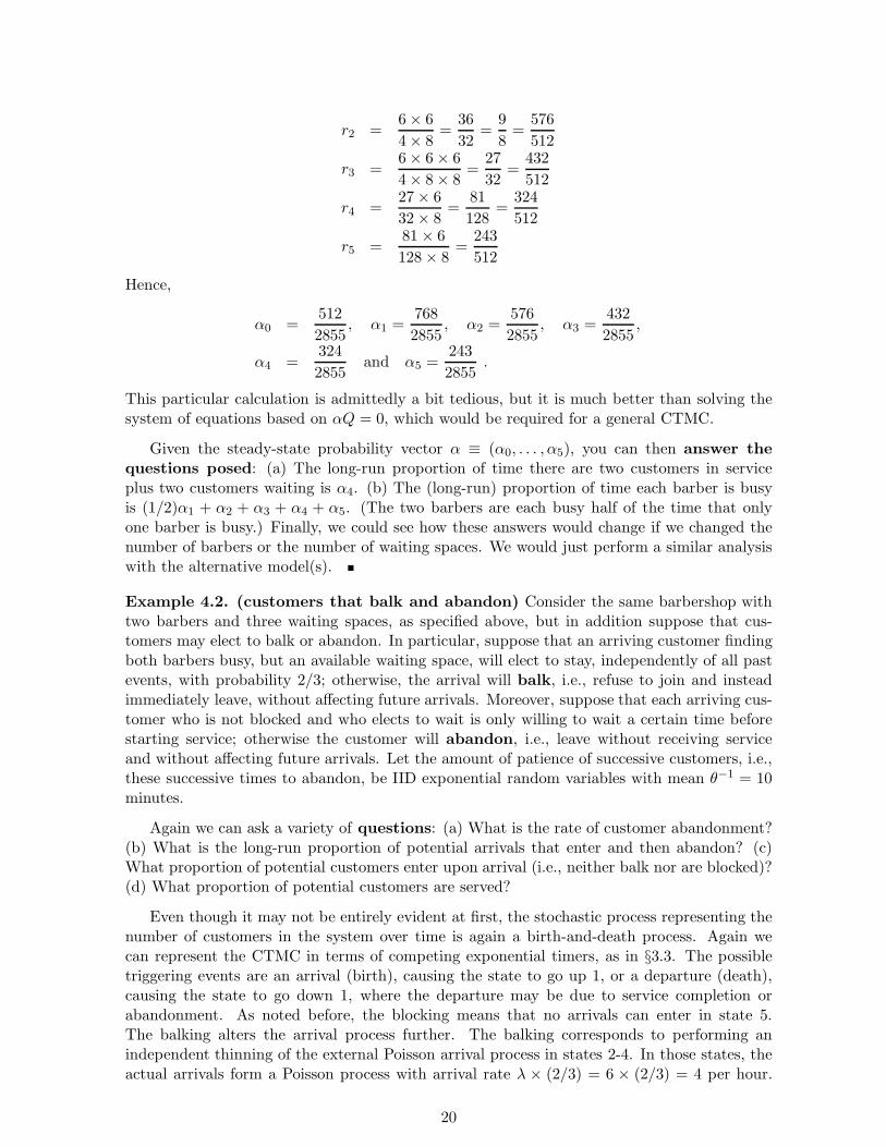
This particular calculation is admittedly a bit tedious, but it is much better than solving thesystem of equations based on αQ = 0, which would be required for a general CTMC.
Given the steady-state probability vector α ≡ (α0, . . . , α5), you can then answer thequestions posed: (a) The long-run proportion of time there are two customers in serviceplus two customers waiting is α4. (b) The (long-run) proportion of time each barber is busyis (1/2)α1 + α2 + α3 + α4 + α5. (The two barbers are each busy half of the time that onlyone barber is busy.) Finally, we could see how these answers would change if we changed thenumber of barbers or the number of waiting spaces. We would just perform a similar analysiswith the alternative model(s).
Example 4.2. (customers that balk and abandon) Consider the same barbershop withtwo barbers and three waiting spaces, as specified above, but in addition suppose that cus-tomers may elect to balk or abandon. In particular, suppose that an arriving customer findingboth barbers busy, but an available waiting space, will elect to stay, independently of all pastevents, with probability 2/3; otherwise, the arrival will balk, i.e., refuse to join and insteadimmediately leave, without affecting future arrivals. Moreover, suppose that each arriving cus-tomer who is not blocked and who elects to wait is only willing to wait a certain time beforestarting service; otherwise the customer will abandon, i.e., leave without receiving serviceand without affecting future arrivals. Let the amount of patience of successive customers, i.e.,these successive times to abandon, be IID exponential random variables with mean θ−1 = 10minutes.
Again we can ask a variety of questions: (a) What is the rate of customer abandonment?(b) What is the long-run proportion of potential arrivals that enter and then abandon? (c)What proportion of potential customers enter upon arrival (i.e., neither balk nor are blocked)?(d) What proportion of potential customers are served?
Even though it may not be entirely evident at first, the stochastic process representing thenumber of customers in the system over time is again a birth-and-death process. Again wecan represent the CTMC in terms of competing exponential timers, as in §3.3. The possibletriggering events are an arrival (birth), causing the state to go up 1, or a departure (death),causing the state to go down 1, where the departure may be due to service completion orabandonment. As noted before, the blocking means that no arrivals can enter in state 5.The balking alters the arrival process further. The balking corresponds to performing anindependent thinning of the external Poisson arrival process in states 2-4. In those states, theactual arrivals form a Poisson process with arrival rate λ × (2/3) = 6 × (2/3) = 4 per hour.
20
Since the interarrival times of a Poisson process have an exponential distribution, there areactive clocks with exponential timers corresponding to the event of a new arrival in states 0-4.The arrival clock in state i has mean 1/λi, where λi is the birth rate to be determined. Thebirth rates in these states are: λ0 = λ1 = λ = 6 per hour and λ2 = λ3 = λ4 = 6 × (2/3) = 4per hour. (The reduction is due to the balking. We have λ5 = 0, because there are no arrivalswhen the system is full.)
Since the service times and times to abandon are independent exponential random variables,the active clocks corresponding to departures also can be represented as exponential randomvariables. As before, there are active clocks with exponential timers corresponding to the eventof a new departure in states 1-5. The departure clock in state i has mean 1/µi, where µi is thedeath rate to be determined. As before, the service rate for each barber is µ = 4 per hour. Sincethe mean time to abandon is 1/θ = 10 minutes for each customer, the individual abandonmentrate is θ = 1/10 per minute or 6 per hour. However, we must remember that the service rateapplies to each server separately, while the abandonment rate applies to each waiting customerseparately. Thus the death rates are µ1 = µ = 4, µ2 = 2µ = 8, µ3 = 2µ + θ = 8 + 6 = 14,µ4 = 2µ + 2θ = 8 + 12 = 20, µ5 = 2µ + 3θ = 8 + 18 = 26. (µ0 = 0.)
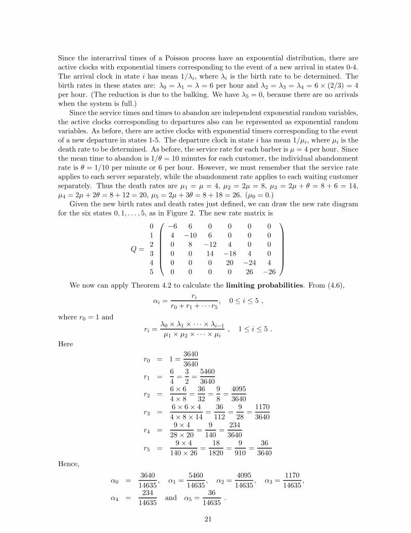
Given the new birth rates and death rates just defined, we can draw the new rate diagramfor the six states 0, 1, . . . , 5, as in Figure 2. The new rate matrix is
We now can apply Theorem 4.2 to calculate the limiting probabilities. From (4.6),
αi =ri
r0 + r1 + · · · r5, 0 ≤ i ≤ 5 ,
where r0 = 1 and
ri =λ0 × λ1 × · · · × λi−1
µ1 × µ2 × · · · × µi, 1 ≤ i ≤ 5 .
Here
r0 = 1 =3640
3640
r1 =6
4=
3
2=
5460
3640
r2 =6× 6
4× 8=
36
32=
9
8=
4095
3640
r3 =6× 6× 4
4× 8× 14=
36
112=
9
28=
1170
3640
r4 =9× 4
28× 20=
9
140=
234
3640
r5 =9× 4
140× 26=
18
1820=
9
910=
36
3640
Hence,
α0 =3640
14635, α1 =
5460
14635, α2 =
4095
14635, α3 =
1170
14635,
α4 =234
14635and α5 =
36
14635.
21
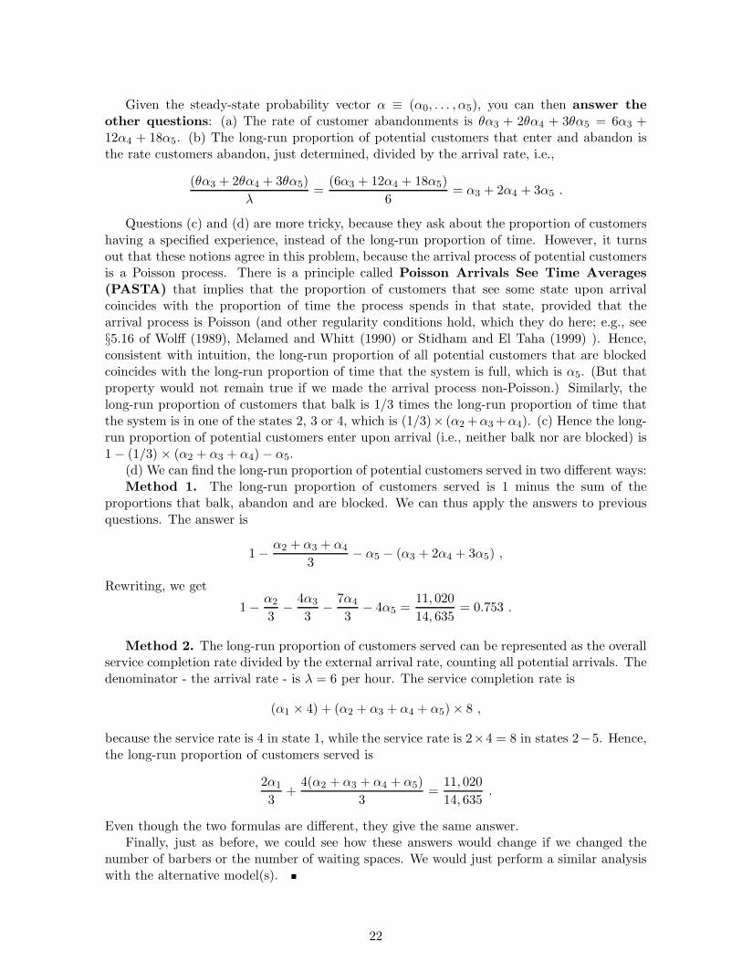
Given the steady-state probability vector α ≡ (α0, . . . , α5), you can then answer theother questions: (a) The rate of customer abandonments is θα3 + 2θα4 + 3θα5 = 6α3 +12α4 + 18α5. (b) The long-run proportion of potential customers that enter and abandon isthe rate customers abandon, just determined, divided by the arrival rate, i.e.,
(θα3 + 2θα4 + 3θα5)
λ=
(6α3 + 12α4 + 18α5)
6= α3 + 2α4 + 3α5 .
Questions (c) and (d) are more tricky, because they ask about the proportion of customershaving a specified experience, instead of the long-run proportion of time. However, it turnsout that these notions agree in this problem, because the arrival process of potential customersis a Poisson process. There is a principle called Poisson Arrivals See Time Averages(PASTA) that implies that the proportion of customers that see some state upon arrivalcoincides with the proportion of time the process spends in that state, provided that thearrival process is Poisson (and other regularity conditions hold, which they do here; e.g., see§5.16 of Wolff (1989), Melamed and Whitt (1990) or Stidham and El Taha (1999) ). Hence,consistent with intuition, the long-run proportion of all potential customers that are blockedcoincides with the long-run proportion of time that the system is full, which is α5. (But thatproperty would not remain true if we made the arrival process non-Poisson.) Similarly, thelong-run proportion of customers that balk is 1/3 times the long-run proportion of time thatthe system is in one of the states 2, 3 or 4, which is (1/3)× (α2 +α3 +α4). (c) Hence the long-run proportion of potential customers enter upon arrival (i.e., neither balk nor are blocked) is1− (1/3) × (α2 + α3 + α4)− α5.
(d) We can find the long-run proportion of potential customers served in two different ways:Method 1. The long-run proportion of customers served is 1 minus the sum of the
proportions that balk, abandon and are blocked. We can thus apply the answers to previousquestions. The answer is
1−α2 + α3 + α4
3− α5 − (α3 + 2α4 + 3α5) ,
Rewriting, we get
1−α2
3−
4α3
3−
7α4
3− 4α5 =
11, 020
14, 635= 0.753 .
Method 2. The long-run proportion of customers served can be represented as the overallservice completion rate divided by the external arrival rate, counting all potential arrivals. Thedenominator - the arrival rate - is λ = 6 per hour. The service completion rate is
(α1 × 4) + (α2 + α3 + α4 + α5)× 8 ,
because the service rate is 4 in state 1, while the service rate is 2×4 = 8 in states 2−5. Hence,the long-run proportion of customers served is
2α1
3+
4(α2 + α3 + α4 + α5)
3=
11, 020
14, 635.
Even though the two formulas are different, they give the same answer.Finally, just as before, we could see how these answers would change if we changed the
number of barbers or the number of waiting spaces. We would just perform a similar analysiswith the alternative model(s).
22
In many applications it is natural to use birth-and-death processes with infinite statespaces. As in other mathematical settings, we primarily introduce infinity because it is moreconvenient. With birth-and-death processes, an infinite state space often simplifies the formof the limiting probability distribution. We illustrate by giving a classic queueing example.
Example 4.3. (the M/M/1 Queue) One of the most elementary queueing models is theM/M/1 queue, which has a single server and unlimited waiting room. As with the M/M/s/rmodel considered in Example 4.1 (with S = 2 and r = 3), customers arrive in a Poissonprocess with rate λ and the service times are IID exponential random variables with mean1/µ. The number of customers in the system at time t as a function of t, say Q(t), is thena birth-and-death process. However, since there is unlimited waiting room, the state space isinfinite.
With an infinite state space, we must guard against pathologies; see §??. In order to havea proper stationary distribution, it is necessary to require that the arrival rate λ be less thanthe maximum possible rate out, µ. Equivalently, we require that the traffic intensity ρ ≡ λ/µbe strictly less than 1.
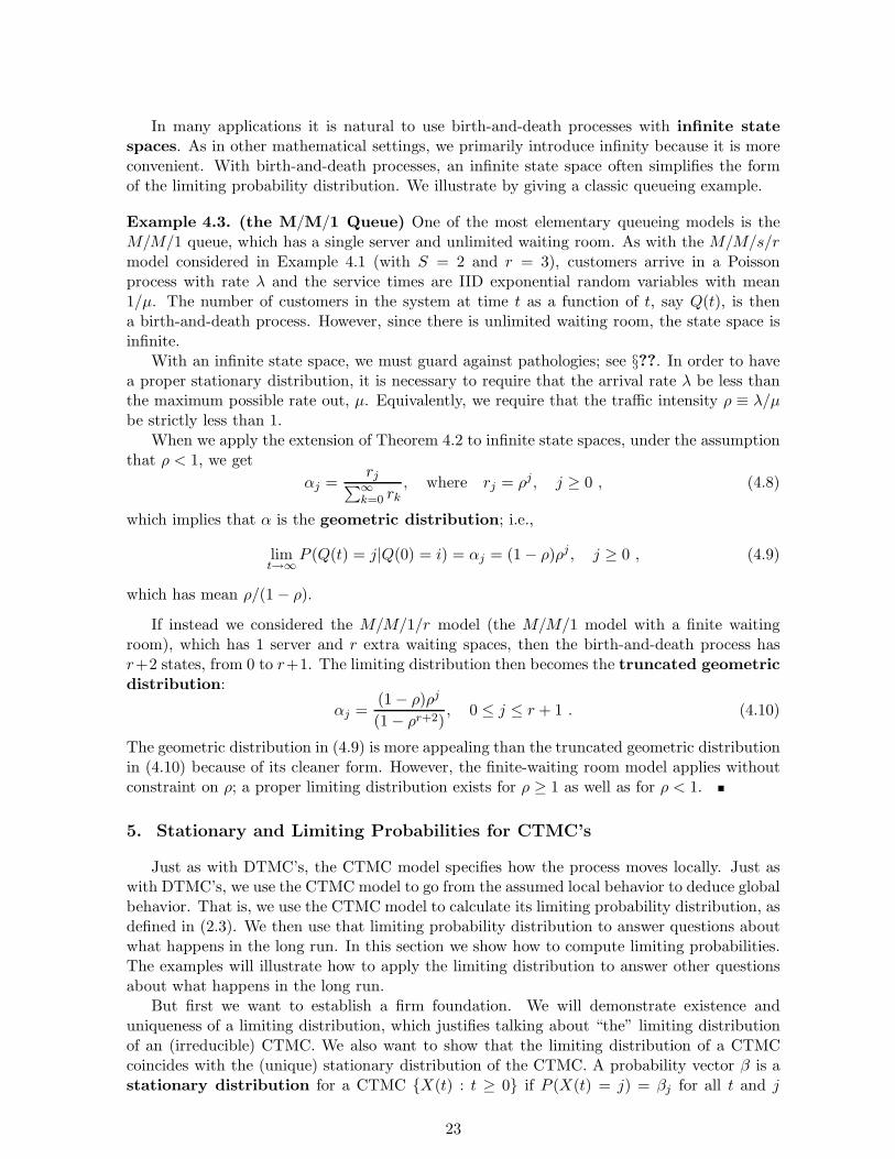
When we apply the extension of Theorem 4.2 to infinite state spaces, under the assumptionthat ρ < 1, we get
αj =rj
∑∞k=0 rk
, where rj = ρj, j ≥ 0 , (4.8)
which implies that α is the geometric distribution; i.e.,
If instead we considered the M/M/1/r model (the M/M/1 model with a finite waitingroom), which has 1 server and r extra waiting spaces, then the birth-and-death process hasr+2 states, from 0 to r+1. The limiting distribution then becomes the truncated geometricdistribution:
αj =(1− ρ)ρj
(1− ρr+2), 0 ≤ j ≤ r + 1 . (4.10)
The geometric distribution in (4.9) is more appealing than the truncated geometric distributionin (4.10) because of its cleaner form. However, the finite-waiting room model applies withoutconstraint on ρ; a proper limiting distribution exists for ρ ≥ 1 as well as for ρ < 1.
5. Stationary and Limiting Probabilities for CTMC’s
Just as with DTMC’s, the CTMC model specifies how the process moves locally. Just aswith DTMC’s, we use the CTMC model to go from the assumed local behavior to deduce globalbehavior. That is, we use the CTMC model to calculate its limiting probability distribution, asdefined in (2.3). We then use that limiting probability distribution to answer questions aboutwhat happens in the long run. In this section we show how to compute limiting probabilities.The examples will illustrate how to apply the limiting distribution to answer other questionsabout what happens in the long run.
But first we want to establish a firm foundation. We will demonstrate existence anduniqueness of a limiting distribution, which justifies talking about “the” limiting distributionof an (irreducible) CTMC. We also want to show that the limiting distribution of a CTMCcoincides with the (unique) stationary distribution of the CTMC. A probability vector β is astationary distribution for a CTMC {X(t) : t ≥ 0} if P (X(t) = j) = βj for all t and j
23
whenever P (X(0) = j) = βj for all j. In general the two notions - limiting distribution andstationary distribution - are distinct, but for CTMC’s there is a unique probability vector withboth properties.
Example 5.1. (distinction between the concepts) Before establishing positive results forCTMC’s, we show that in general the two notions are distinct: there are stationary distributionsthat are not limiting distributions; and there are limiting distributions that are not stationarydistributions.
(a) Recall that a periodic irreducible finite-state DTMC has a unique stationary probabilityvector, which is not a limiting probability vector; the transitions probabilities P k
i,j alternateas k increases, assuming a positive value at most every d steps, where d is the period of thechain. (A CTMC cannot be periodic.)
(b) To go the other way, consider a stochastic process {X(t) : t ≥ 0} with continuousstate space consisting of the unit interval [0, 1]. Suppose that the stochastic process movesdeterministically except for its initial value X(0), which is a random variable taking valuesin [0, 1]. After that initial random start, let the process move deterministically on the unitinterval [0, 1] according to the following rules: From state 0, let the process instantaneouslyjump to state 1. Otherwise, let the process move according to the ODE
X ′(t) ≡dX(t)
dt= −X(t), t ≥ 0 .
Then {X(t) : t ≥ 0} is a Markov process with a unique limiting distribution. In particular,
limt→∞
X(t) = 0 with probability 1 ,
so that the limiting distribution is unit probability mass on 0. However, that limit distributionis not a stationary distribution. Indeed, P (X(t) = 0) = 0 for all t > 0 and all distributionsof X(0). If P (X(0) = 0) = 1, then P (X(t) = e−t for all t) = 1. Even though this Markovprocess has a unique limiting probability distribution, there is no stationary probability vectorfor this Markov process.
But the story is very nice for irreducible finite-state CTMC’s: Then there always exists aunique stationary probability vector, which also is a limiting probability vector. The situationis somewhat cleaner for CTMC’s than for DTMC’s, because we cannot have periodic CTMC’s.That is implied by the following result.
Lemma 5.1. (positive transition probabilities) For an irreducible CTMC, Pi,j(t) > 0 forall i, j and t > 0.
Proof. The argument going forward in time is easy: By Lemma 2.1, if Pi,j(s) > 0, then
Pi,j(s + t) =∑
k
Pi,k(s)Pk,j(t) ≥ Pi,j(s)Pj,j(t) ≥ Pi,j(s)eQj,jt > 0 for all t > 0 ,
because Pj,j(t) is bounded below by the probability of no transition at all from state j in timet, which is eQj,jt. (Recall that Qj,j < 0.) More generally, we apply representation (3.30).Since the CTMC is irreducible, Pi,j(t) > 0 for some t. By representation (3.30), we thushave P k
i,j > 0 for some k, implying that the embedded DTMC with transition matrix P isirreducible. From here on, we argue by contradiction: Suppose that Pi,j(t) = 0 for some t > 0.Then, by representation (3.30), P k
i,j = 0 for all k, which would imply that P is reducible. Sincethat is a contradiction, we must have Pi,j(t) > 0 for all t > 0, as claimed.
24
Theorem 5.1. (existence and uniqueness) For an irreducible finite-state CTMC, thereexists a unique limiting probability vector α; i.e., there exists a unique probability vector αsuch that
limt→∞
Pi,j(t) = αj for all i and j . (5.1)
Moreover, that limiting probability vector α is the unique stationary probability vector, i.e.,if
P (X(0) = j) = αj for all j ,
thenP (X(t) = j) = αj for all j and t > 0 . (5.2)
Proof. We will apply established results for DTMC’s in the setting of the fourth modellingapproach in §3.4; i.e., we will apply uniformization. To do so, we apply representation (3.30).From that representation and Lemma 5.1, it follows immediately that the CTMC is irreducibleif and only if the embedded Markov chain with transition matrix P is irreducible. Assumingthat the CTMC is indeed irreducible, the same is true for that embedded DTMC. By makingλ in (3.26) larger if necessary, we can have Pi,i > 0 for all i, so that the embedded DTMC withtransition matrix P can be taken to be aperiodic as well.
Given that the DTMC with transition matrix P is irreducible and aperiodic, we know thatthe embedded DTMC has a unique stationary distribution π satisfying
π = πP and πe = 1 ,
with the additional property that
P ki,j → πj as k →∞
for all i and j. From representation (3.30), it thus follows that π is also the limiting distributionfor the CTMC; i.e., we have
αj = πj for all j .
Here is a detailed mathematical argument: For any ǫ > 0 given, first choose k0 such that|P k
i,j − πj| < ǫ/2 for all k ≥ k0. Then choose t0 such that P (N(t) < k0) < ǫ/4 for all t ≥ t0.As a consequence, for t > t0,
Moreover, there can be no other stationary distribution, because any stationary distribution ofthe CTMC has to be coincide with the limiting distribution of the DTMC, again by (3.30).
We now turn to calculation. We give three different ways to calculate the limiting distribu-tion, based on the different modelling frameworks. (We do not give a separate treatment forthe competing clocks with exponential timers. We treat that case via the transition rates.) Tosum row vectors in matrix notation, we right-multiply by a column vector of 1′s. Let e denotesuch a column vector of 1′s.
Theorem 5.2. (calculation)
25
(a) Given a CTMC characterized as a DTMC with one-step transition matrix P and tran-sitions according to a Poisson process with rate λ, as in §3.4,
αj = πj for all j , (5.4)
where π is the unique solution to
π = πP and πe = 1 , (5.5)
with P given in (3.27) or, equivalently,
∑
i
πiPi,j = πj for all j and∑
j
πj = 1 . (5.6)
(b) Given a CTMC characterized in terms of a DTMC with one-step transition matrix Pand exponential transition times with means 1/νi, as in §3.1,
αj =(πj/νj)
∑
k(πk/νk), (5.7)
where π is the unique solution to
π = πP and πe = 1 . (5.8)
(c) Given a CTMC characterized by its transition-rate matrix Q, as in §3.2, α is the uniquesolution to
αQ = 0 and αe = 1 (5.9)
or, equivalently,∑
i
αiQi,j = 0 for all j and∑
i
αi = 1 . (5.10)
(d) Given a CTMC characterized by its transition function P (t), perhaps as constructedin §3.4, α is the unique solution to
αP (t) = α for any t > 0 and αe = 1 (5.11)
or, equivalently,∑
i
αiPi,j(t) = αj for all j and∑
i
αi = 1 . (5.12)
Proof and Discussion. (a) Exploiting Uniformization. In our proof of Theorem 5.1above, we have already shown that α coincides with π.
(b) Starting with the embedded DTMC. Since Theorem 5.1 establishes the existenceof a unique stationary probability distribution, it suffices to show that the distribution displayedin (5.7) is that stationary distribution. Equivalently, it suffices to show that π = α for α in(5.7), where π is the unique solution to
π = πP and πe = 1 .
26
To see that is the case, observe that αj = cπj/νj for α defined in (5.7). To show that αP = α,observe that
(αP )j =∑
i
αiPi,j = c∑
i
πi
νiPi,j
= c
∑
i,i6=j
πi
νi
Qi,j
λ+
πj
νjPj,j
= c
∑
i,i6=j
πi
νi
(νi
λPi,j
)
+πj
νj
(
1−
∑
i,i6=j νjPj,i
λ
)
= c
∑
i,i6=j
πiPi,j
λ+
πj
νj−
πj∑
i,i6=j Pj,i
λ
= c
(
∑
i
πiPi,j
λ−
πjPj,j
λ+
πj
νj−
πj(1− Pj,j)
λ
)
= c
(
πj
λ−
πjPj,j
λ+
πj
νj−
πj
λ+
πjPj,j
λ
)
= cπj
νj= αj . (5.13)
From (5.7), we see that αe = 1, where e is again a column vector of 1′s. That completes theproof.
We now give a separate direct informal argument (which can be made rigorous) toshow that α has the claimed form. Let Zi,j be the time spend in state i during the jth visitto state i and let Ni(n) be the number of visits to state i among the first n transitions. Thenthe actual proportion of time spent in state i during the first n transitions, say Ti(n), is
Ti(n) =
∑Ni(n)j=1 Zi,j
∑
k
∑Nk(n)j=1 Zk,j
, (5.14)
However, by properties of DTMC’s, n−1Ni(n) → πi with probability 1 as n → ∞. Moreover,by the law of large numbers,
1
n
Ni(n)∑
j=1
Zi,j =
(
Ni(n)
n
)
(
∑Ni(n)j=1 Zi,j
Ni(n)
)
→ πiE[Zi,j ] = πi/νi as n→∞ . (5.15)
Thus, combining (5.14) and (5.15), we obtain
Ti(n)→(πi/νi)
∑
k(πk/νk)as n→∞ , (5.16)
supporting (5.7). For a full proof, we need to show that this same limit holds at arbitrarytimes t as t→∞. It is intuitively clear that holds, but we do not prove that directly.
(c) Starting with the transition rates. We give several different arguments, fromdifferent perspectives, to show that α is characterized as the unique solution of αQ = 0 withαe = 1.
27
We first apply a rate-conservation principle: In steady state, the rate of transitions intostate j has to equal the rate of transitions out of state j, for each state j. The steady-staterate of transitions into state j is
∑
i,i6=j
αiQi,j
for the limiting probability vector α to be determined, while the steady-state rate of transitionsout of state j is
∑
i,i6=j
αjQj,i = −αjQj,j .
Setting these two steady-state rates equal yields
∑
i
αiQi,j = 0 ,
which, when applied to all j, is equivalent to αQ = 0 in matrix notation.
Alternatively, we can start from the ODE’s. From Theorem 5.1, we know that Pi,j(t)→αj as t → ∞ for all i and j. Thus the right side of the backwards ODE P ′(t) = QP (t)converges, which implies that
P ′i,j(t) =∑
k
Qi,kPk,j(t)→∑
k
Qi,kαj as t→∞ .
However, since∑
k Qi,k = 0 for all i,
P ′i,j(t)→ 0 as t→∞ for all i and j .
When we apply these established limits for P (t) and P ′(t) in the forward ODE, P ′(t) =P (t)Q, we immediately obtain the desired 0 = αQ, where αe = 1.
We can instead work with the DTMC transition matrix P . From (3.20) and (3.27), wesee that
Q = λ(P − I) . (5.17)
Multiply on the left by α in (5.17) to get
αQ = λ(
αP − α)
,
which implies that αQ = 0 if and only if αP = α.
(d) Starting with the transition function P (t). This final characterization is similarto part (a). Apply the explicit expression for P (t) in (3.30) with the expression P = λ−1Q+ Ito deduce that αQ = 0 if and only if αP (t) = α.
To illustrate, we now return once more to Examples 3.1 and 3.2.
Example 5.2. (Pooh Bear and the Three Honey Trees Revisited ) In Example 3.1the CTMC was naturally formulated as a DTMC with exponential transition times, as in thefirst modelling approach in §3.1. We exhibited the DTMC transition matrix P and the meantransition times 1/νi before. Thus it is natural to apply Theorem 5.2 (b) in order to calculatethe limiting probabilities. From that perspective, the limiting probabilities are
αj =πj(1/νj)
∑
k πk(1/νk),
28
where the limiting probability vector π of the discrete-time Markov chain with transition matrixP is obtained by solving π = πP with πe = 1, yielding
π = (8
17,
4
17,
5
17) .
Then final steady-state distribution, accounting for the random holding times, is
α = (1
2,1
4,1
4) .
We were then asked to find the limiting proportion of time that Pooh spends at each ofthe three trees. Those limiting proportions coincide with the limiting probabilities. That canbe demonstrated by applying the renewal-reward theorem from renewal theory.
Example 5.3. (Copier Maintenance Revisited Again) Let us return to Example 3.2 andconsider the question posed there: What is the long-run proportion of time that each copieris working and what is the long-run proportion of time that the repairman is busy? To haveconcrete numbers, suppose that the failure rates are γ1 = 1 per month and γ2 = 3 per month;and suppose the repair rates are β1 = 2 per month and β2 = 4 per month.
We first substitute the specified numbers for the rates γi and βi in the rate matrix Q in(5.3), obtaining
Then we solve the system of linear equations αQ = 0 with αe = 1, which is easy to dowith a computer and is not too hard by hand. Just as with DTMC’s, one of the equations inαQ = 0 is redundant, so that with the extra added equation αe = 1, there is a unique solution.Performing the calculation, we see that the limiting probability vector is
α ≡ (α0, α1, α2, α(1,2), α(2,1)) =
(
44
129,
16
129,
36
129,
24
129,
9
129
)
.
Thus, the long-run proportion of time that copier 1 is working is α0 + α2 = 80/129 ≈ 0.62,while the long-run proportion of time that copier 2 is working is α0 +α1 = 60/129 ≈ 0.47. Thelong-run proportion of time that the repairman is busy is α1 + α2 + α(1,2) + α(2,1) = 1− α0 =85/129 ≈ 0.659,
Now let us consider an alternative repair strategy: Suppose that copier 1 is moreimportant than copier 2, so that it is more important to have it working. Toward that end,suppose the repairman always work on copier 1 when both copiers are down. In particular,now suppose that the repairman stops working on copier 2 when it is down if copier 1 alsosubsequently fails, and immediately shifts his attention to copier 1, returning to work on copier2 after copier 1 has been repaired. How do the long-run proportions change?
With this alternative repair strategy, we can revise the state space. Now it does suffice touse 4 states, letting the state correspond to the set of failed copiers, because now we knowwhat the repairman will do when both copiers are down; he will always work on copier 1. Thusit suffices to use the single state (1, 2) to indicate that both machines have failed. There now
29
Revised Rate Diagram
(1,2)
2
0
1
1
2
2
1
1
1
2
= rate copier j fails, = rate copier j repairedjj
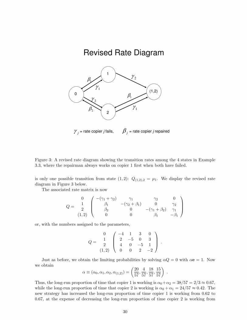
Figure 3: A revised rate diagram showing the transition rates among the 4 states in Example3.3, where the repairman always works on copier 1 first when both have failed.
is only one possible transition from state (1, 2): Q(1,2),2 = µ1. We display the revised ratediagram in Figure 3 below.
The associated rate matrix is now
Q =
012
(1, 2)
−(γ1 + γ2) γ1 γ2 0β1 −(γ2 + β1) 0 γ2
β2 0 −(γ1 + β2) γ1
0 0 β1 −β1
or, with the numbers assigned to the parameters,
Q =
012
(1, 2)
−4 1 3 02 −5 0 34 0 −5 10 0 2 −2
.
Just as before, we obtain the limiting probabilities by solving αQ = 0 with αe = 1. Nowwe obtain
α ≡ (α0, α1, α2, α(1,2)) =
(
20
57,
4
57,18
57,15
57
)
.
Thus, the long-run proportion of time that copier 1 is working is α0+α2 = 38/57 = 2/3 ≈ 0.67,while the long-run proportion of time that copier 2 is working is α0 + α1 = 24/57 ≈ 0.42. Thenew strategy has increased the long-run proportion of time copier 1 is working from 0.62 to0.67, at the expense of decreasing the long-run proportion of time copier 2 is working from
30
0.47 to 0.42. The long-run proportion of time the repairman is busy is 1−α0 = 37/57 ≈ 0.649,which is very slightly less than before.
We conclude by making some further commentary. We might think that the revisedstrategy is wasteful, because the repairman quits working on copier 2 when copier 1 fails aftercopier 2 previously failed. By shifting to work on copier 1, we might think that the repairmanis being inefficient, “wasting” his expended effort working on copier 2, making it more likelythat both copiers will remain failed. In practice, under other assumptions, that might indeedbe true, but here because of the lack-of-memory property of the exponential distribution, theexpended work on copier 2 has no influence on the remaining required repair times. From apure efficiency perspective, it might be advantageous to give one of the two copiers priority atthis point, but not because of the expended work on copier 2. On the other hand, we mightprefer the original strategy from a “fairness” perspective. In any case, the CTMC model lets usanalyze the consequences of alternative strategies. As always, the relevance of the conclusionsdepends on the validity of the model assumptions. But even when the model assumptions arenot completely realistic or not strongly verified, the analysis can provide insight.
6. Reverse-Time CTMC’s and Reversibility
Just as for DTMC’s, an important concept for CTMC’s is reversibility. A stochastic process{X(t) : −∞ < t <∞} is said to be reversible if it has the same probability law as {X(−t) :−∞ < t <∞}. Thus a CTMC is reversible if we get the same CTMC if we run time backwards.
Just as for DTMC’s, we can start by constructing the reverse-time CTMC associatedwith a given CTMC with transition-rate matrix Q and transition function P (t). We obtainthe reverse-time Markov chain from the original (forward) CTMC by reversing time. Thereverse-time transition probabilities describe where the process came from instead of where itis going. That is, we let
←P i,j (t) ≡ P (X(s) = j|X(s + t) = i) . (6.1)
We can then then apply basic properties of conditional probabilities to express these reverse-time transition probabilities in terms of given forward-time transition probabilities; i.e.,
←P i,j (t) ≡ P (X(s) = j|X(s + t) = i) =
P (X(s) = j,X(s + t) = i)
P (X(s + t) = i)=
P (X(s) = j)Pj,i(t)
P (X(s + t) = i).
(6.2)Unfortunately, however, when we do this, we see that in general we do not obtain bonafide
Markov transition probabilities; if we sum over j in (6.2), the transition probabilities do notnecessarily sum to 1, as required. We need to assume more. What we assume in addition is thatthe Markov chain is in equilibrium. That is, we assume that the given (forward) CTMCwith transition function P (t) is irreducible with initial distribution equal to its stationarydistribution α.
Since many reversible processes have infinite-state space, we henceforth allow an infi-nite state space. We assume that the CTMC is irreducible, regular, recurrent and positiverecurrent; see §10. Thus the equation αQ = 0 has a unique solution such that α is a probabilitydistribution.
In this setting we consider the system in equilibrium by letting P (X(t) = j) = αj for all t.Under this extra equilibrium condition, equation (6.2) can be expressed as
←P i,j (t) ≡ P (X(s) = j|X(s + t) = i) =
P (X(s) = j,X(s + t) = i)
P (X(s + t) = i)=
αjPj,i(t)
αi. (6.3)
31
Theorem 6.1. (reverse-time CTMC) If an positive recurrent irreducible CTMC is put inequilibrium by letting its initial distribution be its stationary distribution α, then the transitionprobabilities in (6.3) are bonafide transition probabilities, with the same stationary probabilitydistribution α, and the stochastic process satisfies the reverse-time Markov property
P (X(s) = j|X(s + t) = i,X(u) = iu, u ∈ Au ⊆ (s + t,∞)) = P (X(s) = j|X(s + t) = i)
≡←P i,j (t) . (6.4)
The reverse-time Markov property in (6.4) says that the conditional probability of a “past”state j at time s, given the “present” state i at time s + t plus the states at “future” times uin the set Au depends only on the present state i at time s + t.
Proof. First it is clear that the alleged transition probabilities in (6.3) are nonnegative.
Since αP (t) = α for each t, by Theorem 5.2 (d), the row sums of←P now do indeed sum to 1,
as required. To see that the Markov property in (6.4) does indeed hold, apply properties ofconditional probabilities to rewrite (6.4) as
P (X(s) = j|X(s + t) = i,X(u) = iu, u ∈ Au ⊆ (s + t,∞))
=P (X(s) = j,X(s + t) = i,X(u) = iu, u ∈ Au ⊆ (s + t,∞))
P (X(s + t) = i,X(u) = iu, u ∈ Au ⊆ (s + t,∞))
=P (X(s) = j)Pj,i(t)P (X(u) = iu, u ∈ Au ⊆ (s + t,∞)|X(s + t) = i)
P (X(s + t) = i)P (X(u) = iu, u ∈ Au ⊆ (s + t,∞)|X(s + t) = i)
=P (X(s) = j)Pj,i(t)
P (X(s + t) = i)=
αjPj,i(t)
αi,
where in the last line we have first canceled the common term P (X(u) = iu, u ∈ Au ⊆(s + t,∞)|X(s + t) = i) from the numerator and the denominator and then exploited theequilibrium property.
From (6.3), we see right away (by looking at the derivative at 0) that the reverse-timeCTMC associated with a CTMC having transition-rate matrix Q itself has transition-rate
matrix←Q, where
←Qi,j=
αjQj,i
αi. (6.5)
Note that any irreducible CTMC in equilibrium (initialized with its stationary distribution
α) has an associated reverse-time CTMC with transition-rate matrix←Q. But that does not
make the CTMC reversible. That is a stronger property: A CTMC is said to be time-reversibleor just reversible if the reverse-time CTMC coincides with the original CTMC in equilibrium,
i.e., if←Q= Q or, equivalently, if
αiQi,j = αjQj,i for all i and j . (6.6)
For CTMC’s, reversibility as defined at the beginning of this section is equivalent to equa-tions (6.6). From a rate-conservation perspective, reversibility holds for a CTMC if and only ifthe steady-state rate of transitions from state i to state j equals the steady-state rate of tran-sitions from state j to state i for all states i and j. Thus reversibility is characterized by thedetailed-balance equations in (6.6), which are generalizations of the detailed-balance equa-tions for birth-and-death processes in (4.3). We summarize these properties in the followingtheorem.
32
Theorem 6.2. (reversibility of CTMC’s) A CTMC with transition rate matrix Q is re-versible with stationary probability vector α if and only if the detailed balance equations in (6.6)hold.
Proof. We have seen that the detailed balance equations in (6.6) imply reversibility, giventhat α is the stationary vector. Summing those equations on either i or j gives αQ = 0,implying that α must in fact be the stationary probability vector.
As a consequence, we immediately have the following result.
Theorem 6.3. (reversibility of birth-and-death processes) All birth-and-death processesare reversible.
By the statement in Theorem 6.3, we mean that the birth-and-death process is reversibleprovided that it has a stationary probability vector α and is initialized by that stationary prob-ability vector α.
We now observe that reversibility is inherited by truncation. We say that a CTMC withstate space S and rate matrix Q is truncated to the subset A ⊂ S if we disallow all transitionsout of the subset A; i.e., if we set Qi,j = 0 for i ∈ A and j ∈ S −A. We obtain a new CTMC
with state space A by letting Q(A)i,j = Qi,j for all i and j in A with i 6= j and Q
(A)i,i = −
∑
j∈A Qi,j
for all i ∈ A.
Theorem 6.4. (truncation) If a reversible CTMC with rate matrix Q and stationary prob-ability vector α is truncated to a subset A, yielding the rate matrix Q(A) defined above, andremains irreducible, then the truncated CTMC with the rate matrix Q(A) is also reversible andhas stationary probability vector
α(A)j =
αj∑
k∈A αk, for all j ∈ A . (6.7)
Proof. It is elementary that the truncated CTMC with the probability vector α(A) in (6.7)satisfies the detailed balance equations in (6.6) if the original CTMC does, which holds byTheorem 6.2.
We have seen an instance of Theorem 6.3 when we looked at the M/M/1/r queueing modelin (4.10), following Example 4.3.
We now apply reversibility to get something new and interesting. For that, we considerthe M/M/s queue with s servers, unlimited waiting room, Poisson arrival process with arrivalrate λ and IID exponential service times with mean 1/µ. The number in system over time isa birth-and-death process with constant birth rate λ and death rates µj = min {j, s}µ. Sincethere is an infinite state space, we require that ρ ≡ λ/sµ < 1 in order to have a proper limitingdistribution.
Theorem 6.5. (departures from an M/M/s queue) The departure process from an M/M/squeue in equilibrium (with ρ ≡ λ/sµ < 1) is a Poisson process with departure rate equal to thearrival rate λ.
Proof. Having ρ ≡ λ/sµ < 1 ensures that a proper limiting probability vector α exists.Put the system in equilibrium by letting the initial distribution be that limiting distribution.By Theorem 6.3, the CTMC is reversible. Thus, in equilibrium, the process counting thenumber of customers in the system at any time in reverse time has the same probability law as
33
the original process. However, reversing time changes departures (jumps down) into arrivals(jumps up) and vice versa. So the departures must form a Poisson process with rate λ.
Theorem 6.5 is quite remarkable. It takes some effort to even directly show that thetime between successive departures in an M/M/1 queue in equilibrium has an exponentialdistribution with mean 1/λ. That is an instructive exercise.
We can do more: We can establish an even more surprising result. Let Q(t) be the number insystem at time t, either waiting or being served, and let D(t) count the number of departuresin the interval [0, t]. We can show that the distribution of the queue length at time t isindependent of the departures prior to time t, for the M/M/s queue in equilibrium!
Theorem 6.6. (more about departures from an M/M/s queue) For an M/M/s queuein equilibrium (with ρ ≡ λ/sµ < 1), the number in system at time t, Q(t), is independent of{D(s) : 0 ≤ s ≤ t}, the departure process before time t.
Proof. Just as for Theorem 6.5, having ρ ≡ λ/sµ < 1 ensures that a proper limiting proba-bility vector α exists. As before, put the system in equilibrium by letting the initial distributionbe the limiting distribution. By Theorem 6.3, the CTMC is reversible. Thus, in equilibrium,the process in reverse time has the same probability law as the original process. With any oneordering of time, the arrival process after time t is independent of the queue length at time t.by the independent-increments property of the Poisson process. Since arrivals and departuresswitch roles when we reverse time, we deduce the asserted conclusion as well.
We now go on to consider networks of queues. We first combine Theorems 6.5 and 6.6with Example 4.3 to obtain the limiting distribution for the number of customers at eachstation for two or more single-server queues in series. In particular, consider an M/M/1 modelwith arrival rate λ and service rate µ1, where ρ1 ≡ λ/µ1 < 1. Let all departures from thisM/M/1 queue proceed next to a second single-server queue with unlimited waiting room andIID exponential service times with individual service rate µ2, where also ρ2 ≡ λ/µ2 < 1. Thismodel is often referred to as the M/M/1→ /M/1 tandem queue. Let Qi(t) be the number ofcustomers at station i at time t, either waiting or being served.
Theorem 6.7. (the limiting probabilities for then M/M/1→ /M/1 tandem queue)For the M/M/1 → /M/1 tandem queue in equilibrium (with ρi ≡ λ/sµi < 1 for each i), thedeparture processes from the two queues are Poisson processes with rate λ and
limt→∞
P (Q1(t) = j1, Q2(t) = j2) = (1− ρ1)ρj11 (1− ρ2)ρ
j22 for all j1 and j2 . (6.8)
Theorem 6.7 concludes that the limiting probabilities for the two queues in series are thesame as for two independent M/M/1 queue, each with the given arrival rate λ. (However,the two stochastic processes {Q1(t) : t ≥ 0} and {Q2(t) : t ≥ 0}. starting in equilibrium, arenot independent. The result is for a single time t.) We say that the limiting distribution hasproduct form. That product form means that the two marginal distributions are independent.
Proof. Suppose that we initialize the system with the alleged limiting probability distribu-tion. Since it is the product of two geometric distributions, the two marginal distributionsare independent. Hence we can first focus on the first queue. By Theorem 6.5, the depar-ture process from this first queue is Poisson with rate λ. Hence, the second queue by itselfis an M/M/1 queue in equilibrium. Hence each queue separately has the displayed geometricstationary distribution, which coincides with its limiting distribution. Now, considering thesystem in equilibrium, by Theorem 6.6, at any time t, the random number Q1(t) is indepen-dent of the departure process from the first queue up to time t. That implies that Q2(t) and
34
Q1(t) must be independent for each t, which implies the product-form limiting distribution in(6.8).
Note that the entire M/M/1→ /M/1 tandem queue is not itself reversible; it is possibleto go from state (i, j) to state (i − 1, j + 1) (with a departure from queue 1), but it is notpossible to go back. So the detailed-balance conditions in (6.6) cannot hold. We establishedTheorem 6.7 by exploiting the reversibility of only the first station by itself. However, thereis an alternative way to prove Theorem 6.7 exploiting only reverse-time CTMC’s, which hasother applications, e.g., to treat networks of Markovian queues that are not acyclic (do nothave flow in one direction only).
Theorem 6.8. (Kelly’s Lemma: exploiting reverse-time chains without reversibil-ity) Let Q be the transition-rate matrix of an irreducible CTMC. If we can find numbers αj
and←Qi,j such that
αiQi,j = αj
←Qj,i for all i 6= j (6.9)
and
−Qi,i ≡∑
j,j 6=i
Qi,j =∑
j,j 6=i
←Qi,j≡ −
←Qi,i for all i , (6.10)
then←Qi,j are the transition rates for the reverse-time CTMC associated with Q and α is the
limiting probability vector for both CTMC’s.
Proof. Add over i with i 6= j in (6.9) and apply (6.10) to get
∑
i,i6=j
αiQi,j =∑
i,i6=j
αj
←Qj,i= αj
∑
i,i6=j
Qj,i ,
which implies that αQ = 0. Hence α is the limiting distribution for the CTMC with transition-
rate matrix Q. Consequently,←Qi,j are the transition rates associated with the reverse-time
CTMC based on Q in equilibrium. That implies (by summing on j in (6.9)) that α is thelimiting distribution for the reverse-time CTMC as well.
We now apply Theorem 6.8 to give an alternative proof of Theorem 6.7, which again hasthe advantage that it does not require directly solving the equation αQ = 0.
Alternative proof of Theorem 6.7. As for many harder problems, the first step is toguess the form of the limiting distribution; i.e., we guess that α has the product form in (6.8).We then guess that the reverse-time CTMC should be itself a M/M/1→ /M/1 tandem queuewith arrival rate λ and the given service rates. Going forward from state (i, j), we have threepossible transitions: (1) to state (i + 1, j) due to an arrival, (2) to state (i − 1, j + 1) due todeparture from queue 1 and (3) to (i, j − 1) due to departure from queue 2. We have possibleflows in the other direction for the reverse-time CTMC to state (i, j) in three possible ways:(1) from state (i + 1, j) due to a departure from queue 1 (in original order), (2) from state(i− 1, j + 1) due to departure from queue 2 and (3) to (i, j − 1) due to an arrival from outsideat queue 2. We thus have three equations to check in order to verify (6.9):
(1− ρ1)ρi1(1− ρ2)ρ
j2λ = (1− ρ1)ρ
i+11 (1− ρ2)ρ
j2µ1
(1− ρ1)ρi1(1− ρ2)ρ
j2µ1 = (1− ρ1)ρ
i−11 (1− ρ2)ρ
j+12 µ2
(1− ρ1)ρi1(1− ρ2)ρ
j2µ2 = (1− ρ1)ρ
i1(1− ρ2)ρ
j−12 λ , (6.11)
35
which are easily seen to be satisfied. It is also easy to see that (6.10) holds. For a state (i, j)with i > 0 and j > 0, the total rate out to a new state is λ + µ1 + µ2, corresponding to thepossibilities of an arrival or a service completion at one of the two queues. For the state (0, j)with j > 0, the total rate out to a new state is λ + µ2 in both cases, excluding the possibilityof a service completion from queue 1 in both cases. The case (i, 0) is similar. For the state(0, 0), the total rate out to new states is λ in both cases, corresponding to an arrival.
7. Open Queueing Networks (OQN’s)
A minor variation of the argument we have just used to prove Theorem 6.7 for tandem queues byapplying Theorem 6.8 (Kelly’s lemma) applies to treat a general Markovian open networkof single-server queues (OQN), a special case of a Jackson QN. We give the highlights, butwe only begin to introduce the rich theory of queueing networks; e.g., see Chen and Yao (2001),Kelly (1979), Sauer and Chandy (1981), Serfozo (1999), van Dijk (1993), Walrand (1988) andWhittle (1986).
7.1. The Model
Let there be m single-server queues, each with unlimited waiting room. Let there be an externalPoisson arrival process at queue i with rate λe,i, where λe,i ≥ 0 and λe,i > 0 for at least onei. Let the service times at queue i be exponential with mean 1/µi. Let the arrival processesbe mutually independent. Let all the service times be mutually independent and independentof the arrival processes. Let there be Markovian routing, independent of the arrival andservice processes; i.e., let each customer, immediately after completing service at queue i, gonext to queue j with probability Pi,j, independently of all previous events. Let each customerdepart from the network from queue i with probability 1 −
∑mj=1 Pi,j . If we include outside
of the network as a single state m + 1, then the routing is characterized by a DTMC. In thisrouting DTMC we assume that Pm+1,m+1 = 1, making the outside state absorbing. Moreover,we assume that all other states are transient states. That is, we assume that each arrivingcustomer will eventually depart from the system.
Consider the vector valued process Q(t) ≡ (Q1(t), Q2(t), . . . , Qm(t)), where Qi(t) is thenumber of customers at queue i, either waiting or being served, at time t. It is easy to seethat the stochastic process {Q(t) : t ≥ 0} is a CTMC. The possible events are an arrival fromoutside or a service completion at one of the m queues. Those all governed by the specifiedrates. We will show that this CTMC also has a product-form limiting distribution, underregularity conditions. Given the possibility of feedback now, it is even more remarkable thatthe marginal distributions of the limiting probability distribution should be independent.
7.2. The Traffic Rate Equations and the Stability Condition
To characterize the limiting behavior, we first need to find the total arrival rate at eachqueue, i.e., the sum of the external and internal arrival rates. In order to find the total arrivalrate to each queue, we need to solve a system of linear equations, the traffic-rate equations:
λj = λe,j +
m∑
i=1
λiPi,j for 1 ≤ j ≤ m , (7.1)
or, equivalently, in matrix notation,
Λ = Λe + ΛP , (7.2)
36
which implies thatΛ = Λe(I − P )−1 . (7.3)
The inverse (I − P )−1 is the fundamental matrix of the absorbing routing DTMC.In order for the solution of the traffic-rate equations to be valid total arrival rates, we have
to be sure that the net arrival rate is less than the maximum possible service rate at eachqueue. As before, let the traffic intensity at queue j be
ρj =λj
µj, 1 ≤ j ≤ m . (7.4)
We assume that ρj < 1 for all j, 1 ≤ j ≤ m.
7.3. The Limiting Product-Form Distribution
With those assumptions, the CTMC {Q(t) : t ≥ 0} has a product-form limiting distribution.
Theorem 7.1. (Markovian open network of single-server queues) Consider the Marko-vian open network of single server queues defined above, where the inverse (I − P )−1 is welldefined for the routing matrix P and ρi < 1 for each i. Then the limiting distribution hasproduct form, with geometric marginals of the M/M/1 queue; i.e.,
limt→∞
P (Q(t) = (j1, . . . , jm)) = α(j1, . . . , jm) =
m∏
k=1
(1− ρk)ρjk
k . (7.5)
Proof. A direct proof is to guess that the solution if of product form, as in (7.5), and thensimply verify that αQ = 0. That verification step is simplified by applying Theorem 6.8. To do
so, we need to define the candidate reverse-time CTMC with transition rates←Q. Just as with
Theorem 6.7, we guess that the reverse-time CTMC itself corresponds to an open network ofsingle-server queues, with the same service-time distributions at the queues, but we need to
guess the appropriate external arrival rates←λe,i and routing probabilities
←P i,j. The idea is to
guess those quantities by seeing what is required to have the flow rates balance in equilibrium.First, the flow rate through each queue should be the same in either direction, so we should
have←λ i= λi for all i . (7.6)
Next, the reverse-time external arrival rate at queue i should be equal to the forward-timedeparture rate from queue i, i.e.,
←λe,i= λi(1−
m∑
j=1
Pi,j) for all i . (7.7)
To complete the construction, note that the stationary flow from queue i to queue j in forwardtime should equal the stationary reverse flow in reverse time, i.e.,
λiPi,j =←λj
←P j,i . (7.8)
As a consequence, we have←P j,i=
λiPi,j←λ j
. (7.9)
37
Combining equations (7.6), (7.7) and (7.9), we have defined the reverse-time model elements←λe,i,
←λ i and
←P j,i for all i and j in terms of the corresponding forward-time modelling elements.
For the reverse-time queueing network, we should have an analog of the traffic-rate equa-tions in (7.10) in reverse time, namely,
←λ j=
←λe,j +
m∑
i=1
←λ i
←P i,j for 1 ≤ j ≤ m , (7.10)
or, equivalently, in matrix notation,
←Λ=←Λe +
←Λ←P . (7.11)
And, indeed, it is easy to check that these reverse-time traffic rate equations are valid, byapplying the definitions above.
Just as for the tandem OQN in Theorem 6.7, we assume that the reverse-time OQN hasindependent Poisson arrival processes at each queue and Markovian routing. The external
arrival rate at queue j is then←λe,j satisfying (7.7). The routing probabilities are
←P j,i as given
in (7.9). It then remains to verify that these guesses yield the right answer; i.e., we need toverify equations (6.9) and (6.10) in this setting, remembering that the states now correspondto m-tuples (i1, . . . , im). That is straightforward, paralleling the proof of Theorem 6.7. Asbefore, all transitions are triggered by arrivals and service completions (followed by a randomrouting).
From the reverse-time construction just completed, we also can deduce the following corol-lary.
Corollary 7.1. (Output Theorem: departure processes from an OQN) Under theassumptions of Theorem 7.1, the m departure processes from the network from the individualqueues are m independent Poisson processes, with the departure process from queue i havingrate
δi ≡ λi(1−m∑
j=1
Pi,j) . (7.12)
Moreover, the total departure process is a Poisson process with rate
δ ≡m∑
j=1
δj =m∑
j=1
λe,j . (7.13)
Proof. By construction, the external arrival processes to the queues of the reverse-time OQNare independent Poisson processes, just as assumed for the original OQN. However, the arrivalprocesses in the reverse-time OQN coincide with the forward-time departure processes fromthe network, with the specified rates. We only look at those departures that actually leavethe entire network. We do not look at arrivals routed to some other queue.) To completethe proof, it is good to have a characterization of a Poisson process that does not dependon the ordering of time. With our usual “forward thinking,” we think of the arrivals in aninterval [t, t + u], being independent of the process before time t. However, instead it is usefulto characterize the Poisson process as a process with single jumps that has stationary andindependent increments. That characterization applies both forwards and backwards. Thus areverse-time Poisson process necessarily also is a Poisson process. For (7.13), recall that thesuperposition of independent Poisson processes is Poisson with a rate equal to the sum of therates. To see that the total rate in equals the total rate out, as we would expect, compare thesum over i of (7.12) to the sum over j of (7.10).
38
Remark 7.1. (non-Poisson internal flows) While the flows into and out of the network atthe queues are independent Poisson processes, in general the internal flows are not Poissonprocesses, because of the feedback. To illustrate, consider a simple OQN consisting of onesingle-server queue, where each customer after completing service returns to the back of thequeue for an additional service with probability p, independent of the history prior to thatservice completion. If the external arrival rate at that queue is λe, then the net arrival rate isλ = λe/(1 − p). Assume that λ < µ, where µ is the service rate at the queue, so the that thenumber of customers in the system is a positive recurrent CTMC. We now want to see thatthe internal departure process cannot be Poisson.
To see that the departure (service completion) process cannot be Poisson, we observe thatit cannot have independent increments. Consider two successive increments D(t) −D(t − u)and D(t+u)−D(t). As D(t)−D(t−u) increases, the next increment D(t+u)−D(t) is morelikely to be big, because many of of the departures in the interval [t− u, t] we will return foran additional service. To make this effect evident, Suppose that p = 1/2, λe = ǫ and µ = 2, sothat λ = 2ǫ and ρ = ǫ, so that the mean number in the system at any time is ǫ/(1− ǫ). Thenlet ǫ be small. Since the flow rates are very small, P (D(t + u)−D(t) > 1) will be very small,but the conditional probability P (D(t + u) − D(t) > 1|D(t) − D(t − u) = M) can be muchlarger if M is large, because many of the departures in the interval [t− u, t] we will return foran additional service.
7.4. Extensions: More Servers or Different Service Scheduling Rules
We have assumed that each queue has only a single server with the first-come first-served(FCFS) service discipline, but the theory extends to other models for the individual queues.
1. More Servers. First, Theorem 7.1 and Corollary 7.1 extend to Markovian OQN’s withmulti-server queues, where there may be different numbers of servers at each queue. Againwe assume that the service-time distribution is exponential and the FCFS service-schedulingrule is used. Again there is a product-form limiting distribution, but now the marginal steady-state distributions at each queue have the limiting distribution of the M/M/s queue, where s isthe number of servers at that queue. Even more generally, the service-rate at each queue maybe state dependent with a rate depending on the number of customers there. The marginaldistribution is again given by the birth-and-death process steady-state. In all these extensionswe need to assume that the net rate into each queue is strictly less than the maximum rateout, where the rate in is determined by the traffic rate equations. For the M/M/si queue atnode i, the revised traffic intensity is
ρi ≡λi
siµi.
We need ρi < 1 for all i.
2. Non-FCFS Service-Scheduling Rules. Second, Theorem 7.1 and Corollary 7.1extend to Markovian OQN’s with single-server queues but certain special non-FCFSscheduling rules. There are two alternative scheduling rules for single-server queues: processor-sharing (PS) and last-come first-served with preemptive-resume (LCFS-PR). Withthese alternative non-FCFS service-scheduling rules, the steady-state has the insensitivityproperty: The service-time distribution need not be exponential. The successive service timescan be i.i.d. with a general distribution (having finite mean). The product-form steady-statedistribution depends on that general service-time distribution at that queue only through itsmean; the steady state distribution is the same as if it were exponential.
In managing systems with queues, service scheduling can be very important. Thus, theextension to non-FCFS service-scheduling rules has proven to be very useful. The PS service
39
discipline has been extensively used. It serves as a good approximation of the round robin(RR) scheduling rule. With RR and PS, all customers requiring service can be said tobe in service. Customers have service requirements determined upon arrival to the queue.The customer remains at the queue until all its required service has been provided. With PS,at each instant, the available service rate of the server is divided equally among all customersrequiring service at that instant. Hence, in general, unlike FCFS, customers do not depart inthe order they arrive.
The PS scheduling rule is a convenient mathematical approximation for the RR schedulingrule. With the RR rule, only one customer receives service at any time, but the customerstake turns, in a round robin order, each receiving a small fixed quantum of service, untiltheir requirement is met. The customer departs when the initial service requirement is met;otherwise the customer returns to the end of the line, to wait until it can receive the nextquantum of service. Unfortunately, the RR rule, is not so easy to analyze, and does not havethe insensitivity property, so that the PS model is used as an approximation for the RR rule.
The LCFS-PR scheduling rule is less frequently used, but it also leads to the product-formsteady-state distribution with the insensitivity property. With LCFS-PR, all service rate isallocated to the last customer to arrive. Whenever a new arrival comes, that new arrivalreplaces the customer in service, while the customer that was in service goes to the head ofthe queue of waiting customers. However, the partial service provided to each customer is notlost. When a customer who had his service interrupted returns to the server, his service timeresumes where it left off. The remaining requirement is the initial requirement reduced by allservice provided so far. With LCFS-PR, immediately enters service upon arrival and mightcomplete service before another customer arrives. However, customers might have their serviceinterrupted multiple times. Given that the model is stable (the traffic intensity is less than 1at each queue), all customers will eventually be served.
The product-form with the insensitivity property also holds for queues that are infinite-server (IS) queues; then each customer enters service immediately upon arrival. The productform is then the same as if the queue were an M/M/∞ queue, which is covered by the firstextension above. For these three alternative individual queue models – PS, LCFS-PR and IS,the service-time distribution need not be exponential. Nevertheless, the product-form steady-state distribution of the OQN is the same as if the queues were FCFS queues with exponentialservice distributions.
7.5. Steady State in Discrete and Continuous Time
Throughout our study of CTMC’s, we focus on the limiting steady-state probability vectorα, which describes the probability distribution of the model at an arbitrary time in steadystate. It is important to be aware that this same distribution might not be apply at otherspecial times. Indeed, we have already seen in §3.1 and §5 that the steady-state distributionin continuous time, α, is in general different from the steady-state at transition epochs, whichwe have denoted by π; see (3.2) and (5.7).
Similarly, the steady-state distribution at arrival epochs and at departure epochs need notagree with the continuous-time steady-state distribution. However, there is a principle calledPoisson Arrivals See Time Averages (PASTA) that implies that the proportion of cus-tomers that see some state upon arrival coincides with the proportion of time the processspends in that state, provided that the arrival process is Poisson (and other regularity con-ditions hold, which they do here; e.g., see §5.16 of Wolff (1989), Melamed and Whitt (1990)or Stidham and El Taha (1999). In particular, PASTA always holds for a Poisson processindependent of the system, as would be seen by an outside observer, but it also holds for a
40
Poisson process that is part of the system under an additional lack of anticipation assumption.Closely related to PASTA is the arrival theorem, which describes the steady-state seen
be an arrival at a queue in a queueing network. The arrival theorem is valid for internal flowsin the network even though they are not Poisson. In an OQN, the arrivals at a queue seethe steady-state even though the arrival may come on an internal flow that is not Poisson;e.g., see Melamed and Whitt (1990). For associated closed queueing networks, having a fixedpopulation of customers, which we consider next, arrivals see the network with that customerremoved. That is the steady-state distribution for the network with the population reducedby 1.
The connections between stationary distributions for the same system viewed in discreteand continuous time has been studied for more general stochastic processes than Markovprocesses. This issue is at the heart of the theory of stationary point processes and stationarymarked point processes.
8. Closed Queueing Networks (CQN’s)
We obtain a closed queueing network (CQN) from an OQN if we eliminate all external arrivalprocesses from the model and instead assume that there is a fixed number (population) ofcustomers in the system, say N . The resulting model is a Gordon-Newell QN or a closedJackson QN.
8.1. Why Are Closed Models Interesting?
From a modeling perspective, it is natural to wonder why there would be much interest in aCQN, because in most systems customers or jobs arrive from outside, move around and theneventually depart when all required service is complete. At first glance, an OQN seems muchmore natural than a CQN. However, CQN’s have been used extensively, perhaps even morethan OQN’s, especially in models of computer systems.
When closed models are used, people think of a new job replacing an old one whenever theold job has completed its required service. Which model is appropriate depends on what youthink can be directly specified and controlled and what needs to be calculated by analyzing amodel. With some systems, it is natural to think of the population of jobs in the system as theindependent variable, which can be directly specified and controlled, while the throughput(the departure rate of completed service from the network) is the dependent variable, whichneeds to be determined by analyzing a model. That perspective leads to a CQN.
In contrast, with an OQN, the throughput is the independent variable, which is directlyspecified as the total arrival rate (which equals the total departure rate), while the populationis a dependent random variable, which is to be determined, e.g., via its steady-state distributionor the expected value of that steady-state distribution.
However, OQN’s tend to be easier to analyze than CQN’s, especially when more generalnon-Markovian models are contemplated. It thus can be useful to observe that the CQNperspective can be achieved with OQN’s by using the fixed population mean (FPM)method, discussed in Whitt (1984) and §5.5 of Walrand (1988). The idea is to regard theexpected steady-state system population as given, and then do a search over all external arrivalrates to find that external arrival rate that produces the desired mean steady-state total numberin the OQN. For small systems, the performance of the OQN with the FPM method tends tobe very different from the performance of the CQN, because the steady-state number in thesystem tends to be quite variable in the OQN. Surprisingly, however, the performance tendsto be much less in large systems, either with many queues or with a large population. In such
41
larger OQN’s, the variance of the total system population in steady state tends to be relativelysmall compared to the mean.
8.2. A Normalized Product-Form Distribution
Markovian CQN’s can be analyzed much like OQN’s. They are still CTMC’s and Kelly’slemma can still be applied, but there are some significant differences.
As for the OQN, let the CQN have m single-server queues with service rate µi at queue i.As before, let the routing matrix be denoted by P ≡ (Pi,j), but now we assume that it is thetransition matrix of an irreducible DTMC instead of a transient DTMC.
Let the vector of queue lengths (number at each queue, including in service, if any) beQ(t) ≡ (Q1(t), . . . , Qm(t)) and let possible states be vectors n ≡ (n1, . . . , nm), where ni ≥ 0for all i and we impose the CQN population constraint
m∑
i=1
ni = N. (8.1)
Each transition is a service completion combined with a routing of that customer to theend of another queue. In particular, the rate of a service completion at queue i that goesto queue j is µiPi,j for all states n ≡ (n1, . . . , nm) such that ni > 0. To concisely describetransitions among states, let ei be a vector with a 1 in the ith place and 0’s elsewhere TheCTMC {(Q1(t), . . . , Qm(t)) : t ≥ 0} is specified by its rate “matrix.” For any state vector nwith ni > 0, transitions to state vector n− ei + ej occur at rate µiPi,j, i.e., the transition ratesare specified by
Qn,n−ei+ej≡ µiPi,j for all n with ni > 0.
The rate matrix is specified by having
∑
n′
Qn,n′ = 0.
(This is just the vector analog of having all row sums in the rate matrix be 0.) In this setting,we see that the limiting steady-state probability vector is the familiar α ≡ αn ≡ αn1,...,nm suchthat
αQ = 0.
What remains is to show that this steady-state probability vector has a simple modificationof the product form we saw for OQN’s. In particular, it is a normalization of the steady-statedistribution of the OQN to enforce the population constraint in (8.1) above. To character-ize this steady-state distribution, we need the CQN traffic rate equations. Since there areno external arrival processes, instead of (7.10) and (7.11), we have the CQN traffic rateequations
λj =
m∑
i=1
λiPi,j for 1 ≤ j ≤ m, (8.2)
or equivalently, in matrix notation,Λ = ΛP, (8.3)
where Λ ≡ (λ1, . . . , λm) is a 1 × m row vector and P is the usual m ×m Markov transitionmatrix.
We immediately observe that the CQN traffic equations in (11.20) and (11.21) agreeswith the fundamental DTMC equation π = πP , which has a unique solution as a probability
42
vector, because P is the transition matrix for an irreducible m-state DTMC. Hence, the uniquestationary probability vector π is one such solution. However, here there is no reason why theflow rates should sum to 1. Any positive multiple cπ for c > 0 is another solution. Fromthe DTMC theorem, those are the only solutions. This one-parameter family of solutions tothe traffic rate equations does specify the relative arrival rates. The ratio of the flow ratethrough queues i and j necessarily is λi/λj = cπi/cπj , which is the same as πi/πj . So wehave determined the relative traffic rates. The remaining degree of freedom is removed by thepopulation constraint (8.1).
Theorem 8.1. (Markovian closed network of single-server queues) Consider the CQNwith single-server queues defined above, where Λ ≡ (λ1, . . . , λm) is a solution to the traffic rateequations in (11.20) or (11.21). Then the limiting distribution has the normalized product form,
αn ≡ α(n1,n2,...,nm) ≡f(n)
G(N), (8.4)
where
f(n) ≡ f((n1, n2, . . . , nm)) =
m∏
i=1
ρni
i , (8.5)
with ρi ≡ λi/µi, 1 ≤ i ≤ m,
G(N) ≡∑
n:n∈S(N)
f(n) =N∑
n1=0
N−n1∑
n2=0
. . .
N−∑m−1
i=1 ni∑
nm−1=0
f
(
n1, . . . , nm−1, N −m−1∑
i=1
ni
)
(8.6)
and
S(N) ≡ {n ≡ (n1, . . . , nm) : ni ≥ 0 for all i and
m∑
j=1
nj = N}. (8.7)
First Proof. We can apply Theorem 6.8 (Kelly’s lemma). We guess that the reverse-timeCTMC is just another CQN of the same form with the same service rates and the samerelative throughput rates
←−λ i = λi for all i. Then just as in (7.8) and (7.9), we should have
λiPi,j =←λj
←P j,i, so that
←P j,i= λiPi,j/
←λ j. Then, paralleling the proofs of Theorems 6.7 and 7.1,
we can check that the detailed balance equation holds, namely,
αnQn,n−ei+ej= αn−ei+ej
←−Qn−ei+ej ,n, (8.8)
so that the proof is completed by invoking Theorem 6.8.
Second Proof. The difficulty with the first proof is that it is not so clear how to guess theform of the steady-state probability vector α. The second approach is to apply a related OQNto guess the form of the steady-state distribution for the associated CQN.
We construct the OQN by performing a cut on one arc with positive flow. Choose twostates in the CQN where there is positive routing probability in one direction. Without loss ofgenerality, this can be from queue 2 to queue 1, possibly after relabeling the queues. Assumingthat P2,1 > 0, create an associated OQN by making two changes: (i) introduce a Poissonexternal arrival process at queue 1 with small rate ǫ > 0 and (ii) let all flow that would havegone from queue 2 to queue 1 leave the network.
The resulting OQN has total external arrival rate ǫ and thus total departure rate ǫ. Wenow solve the OQN. For sufficiently small ǫ, we will have ρi ≡ λi/µi < 1 at each queue in
43
the OQN. Under that condition, the OQN will have a unique stationary probability vector αsatisfying αQ = 0. In particular, we will have
fOQN(n) ≡ fOQN((n1, . . . , nm)) =m∏
i=1
(1− ρi)ρni
i (8.9)
However this unique invariant measure for the OQN is also an invariant measure for the CQN.Of course, (8.9) is not the same as f(n) in (8.5) because there is the extra term
A ≡
m∏
i=1
(1− ρi), (8.10)
in (8.9), but A in (8.10) is a constant, so both (8.9) and (8.5) are stationary measures for theCQN CTMC, by the same argument given above. The differing constant will be removed bythe normalization. From this point, we can apply Theorem 6.8 (Kelly’s lemma) to completethe proof. This reasoning also leads to formulas (8.4)-(8.7) above.
8.3. Computing the Normalization Constant: The Convolution Algorithm
One difficulty remains: We still need to compute the normalization constant G(N) in (8.6),which is also called the partition function. This can be done by a recursive algorithm, calledthe convolution algorithm or the Buzen algorithm. Let the queues be labeled in order from 1to m. Instead of the notation G(N), now use new notation that counts the number of queues,with the given initial ordering. Let
G(N,m) =∑
{n:n1+n2+···+nm=N}
m∏
i=1
ρni
i , (8.11)
where, as before, ρi ≡ λi/µi, 1 ≤ i ≤ m, with λ ≡ (λ1, . . . , λm) a solution to (11.20).
Theorem 8.2. (Buzen’s convolution algorithm) For any N > 1 and M > 1, the normalizationconstant G(N,m) defined in (8.11) can be solved by the two-dimensional recursion
G(N,m) = g(N,m− 1) + ρmG(N − 1,m). (8.12)
Proof. The first term on the right in (8.12) covers the case in which nm = 0, while the secondcase on the right covers the complementary case in which nm > 0.
An alternative way to compute the normalization constant is to numerically invert itsgenerating function. This approach becomes more important in multi-chain multi-class CQN’swhere there are multiple population constraints, producing normalization constants of theform G(N) = G((N1, . . . , Np)); see Choudhury et al. (1995a). This alternative approach isappealing because the numerical inversion makes it possible to compute any single value G(N)without computing the function for all vectors N ′ with N ′ < N . The generating function canalso be exploited to perform asymptotic approximations.
The generating functions have a remarkably simple form. For the basic model with nor-malization constant G(N) in (8.6), its generating function is defined as
G(z) ≡
∞∑
N=0
G(N)zN . (8.13)
44
Proposition 1. (generating function of the normalization constant) For the CQN above withm single-server queues,
G(z) ≡∞∑
N=0
G(N)zN =m∏
i=1
(1− ρizi)−1. (8.14)
Proof. The main idea is to change the order of summation, which is carried out in the thirdline below. Substituting in G(N) from (8.6) into (8.13), we obtain
G(z) ≡∞∑
N=0
G(N)zN =∞∑
N=0
∑
n∈S(N)
f(n)
zN
=
∞∑
N=0
∑
n∈S(N)
m∏
i=1
ρni
i
zN =
∞∑
N=0
∑
n∈S(N)
m∏
i=1
ρni
i zni
=
∞∑
n1=0
· · ·
∞∑
nm=0
(
m∏
i=1
ρni
i zni
)
=
m∏
i=1
∞∑
n1=0
· · ·
∞∑
nq=0
ρni
i zni
=
m∏
i=1
(1− ρiz)−1 (8.15)
as claimed.
9. Stochastic Loss Models
Another important class of stochastic networks are the loss networks. These can be viewedas generalizations of the classical Erlang loss model. Reversibility also plays a role here. Weillustrate how reversibility can be used to deduce the insensitivity property of the Erlang lossmodel.
9.1. The Erlang Loss Model
This is the Markovian M/M/N/0 queueing model with Poisson arrival process, N servers,exponential service times and no extra waiting space. The number of customers in the system(all in service) is a a finite-state BD process. The birth rates are λk ≡ λ and the death ratesare µk = kµ for an overall arrival rate of λ and an individual service rate of µ. The detailedbalance equations give
αjλ = αj+1(j + 1)µ, (9.1)
so that, by Theorem 4.2,
αj = Gaj
j!, 0 ≤ j ≤ N, (9.2)
where a ≡ λ/µ is the offered load (the expected number of busy servers in the associatedinfinite-server model) and the normalization constant G ≡ G(N) ≡ G(N, a) is chosen so thatthe steady-state probabilities αj sum to 1. Hence
G(N) =
N∑
j=0
aj
j!(9.3)
45
This system can be viewed as a truncation of the associated M/M/∞ infinite-server system,where
G(N) =∞∑
j=0
aj
j!= ea; (9.4)
then the steady-state distribution is Poisson with mean a. (The truncation can be viewed asa consequence of Theorem 6.4.)
The principle performance measure for the Erlang loss model is the steady state blockingprobability experienced by an arrival, which coincides with the steady-state probability αN bythe PASTA property, which can be expressed directly in terms of the normalization constant:
B(N, a) = αN = 1−G(N − 1, a)
G(N, a). (9.5)
For large N and a, it is convenient to calculate the blocking probability B(N, a) by arecursion. The standard recursion is
B(N, a) =aB(N − 1, a)
s + aB(N, a)=
1
1 + [N/aB(N − 1, a)], (9.6)
where B(0, a) ≡ 1 and a ≡ λ/µ is the offered load; see Whitt (2002), where more informationand references can be found.
To understand the application of numerical inversion to calculate normalization constants(partition functions) by inverting their generating functions in more general loss models, weshow how to calculate the generating function here.
Proposition 2. (generating function of the normalization constant) For the M/M/N/0 nor-malization constant G(N) in (10.4), the generating function is
G(z) ≡∞∑
N=0
G(N)zN =eνz
1− z. (9.7)
Proof. We reason as for Proposition 1, changing the order of summation at the end of thefirst line:
G(z) ≡
∞∑
N=0
G(N)zN =
∞∑
N=0
N∑
j=0
νj
j!
zN =
∞∑
j=0
∞∑
N=j
νj
j!zN
=
∞∑
j=0
(νz)j
j!
∞∑
N=j
zN−j =
∞∑
j=0
(νz)j
j!
∞∑
N=0
zN
=
(
1
1− z
) ∞∑
j=0
(νz)j
j!=
eνz
1− z. (9.8)
9.2. Insensitivity in the Erlang Loss Model
The M/M/N/0 Erlang loss model has the insensitivity property; i.e., the same steady statedistribution still holds in the M/GI/N/0 model, having i.i.d. service times with an non-exponential distribution but the same mean. The three concepts reversibility, insensitivity andproduct form are intimately related. There is by now a huge literature, but some issues remaincomplicated.
46
Theorem 9.1. (insensitivity of M/GI/N/0 model) The steady-state distribution of the num-ber of customers in the M/GI/N/0 model depends on the general service-time distribution onlythrough its mean.
We apply a generalization of Theorem 6.1 (Kelly’s lemma) to the case of a non-discrete statespace. We guess the steady-state distribution of the Markov process (to be specified below)and the reverse-time Markov process, and then show that the detailed balance equation holds.By the same elementary reasoning that completes the proof provided that the generalizationof the equation αQ = 0 is still valid. The validity of such characterizations of the steady-state distribution gets much more complicated with non-discrete state spaces, but the ideasare similar. See §4.9 of Ethier and Kurtz (1986) for supporting details for that step. (In thatgreater generality, the rate matrix Q is the generator, often denoted by A. For the generalstate space, it is assumed that A generates a strongly continuous contraction semi-group onan appropriate space and the martingale problem for A is well posed. Then the existence ofa stationary distribution α is equivalent to αQ = 0, expressed as
∫
Af dα = 0 for all f in thecore of A.)
The main line of reasoning is the same as we have been using. The process describingthe system state can be made a continuous-time Markov process (but with uncountable statespace) if we include the ages of the customers in service. A state of this Markov process canbe written as
(n;x) ≡ (n; (x1, x2, . . . , xn)), (9.9)
where, without loss of generality, we take the ages to be expressed in increasing order, so thatx1 < x2 < · · · xn.
The steady-state distribution turns out to be just what we would hope for: The steady-statenumber in system is the same as for the M/M/N/0 model. Given that there are n customersin service, the ages of these service times in process (and the residual lifetimes) in steady stateare independently distributed, each with cdf Ge, the equilibrium excess distribution associatedwith the service-time cdf G, which has density
ge(x) ≡Gc(x)
ES. (9.10)
Taking account of the order requirement on the ages, which introduces the factor n!, we obtainthe steady state distribution of the Markov process.
Theorem 9.2. (steady-state of M/GI/N/0 Markov process) For the M/GI/N/0 model, if theservice-time cdf has a pdf g, then the steady-state distribution is
Proof. We guess that the claim is correct and identify the reverse-time Markov processand apply the generalization of Kelly’s lemma. The reverse-time Markov process is also anM/GI/N/0 Markov process with Poisson arrival process, but in reverse time the forward-time ages become residual lifetimes or excess variables. There are two possible events: (i) anarrival or (ii) a service completion. An arrival takes the state (n;x) into (n + 1; (0, x)) for xof dimension n. A service completion takes the state (n;x) into (n − 1; ei(x)), where x is ofdimension n and ei(x) is the n−1-dimension vector with the ith component of x removed. Letthe hazard rate of the service-time cdf be
h(x) ≡g(x)
Gc(x), x > 0. (9.12)
47
The two detailed flow equations are
α(n;x)λ = α(n + 1; (0, x)) (9.13)
α(n;x)h(xi) = α(n− 1; ei(x))λg(xi) (9.14)
These can be seen to hold, as we now show. First, for (9.13),
α(n + 1; (0, x)) =
(
λ
(n + 1)µ
)
(n + 1)Ge(0)× α(n;x), (9.15)
but(
λ
(n + 1)µ
)
(n + 1)Ge(0) = λ, (9.16)
so that (9.13) holds.We no turn to (9.14). The second formula in (9.14) becomes
α(n;x)h(xi) = α(n;x)g(xi)
Gc(xi)(9.17)
whileα(n;x)
α(n− 1; ei(x))=
(
λ
nµ
)
nge(xi) =λge(xi)
µ= λGc(xi). (9.18)
Applying (9.17) and (9.18), we see that indeed (9.14) holds.
9.3. Stochastic Loss Networks
Stochastic loss networks are generalizations of the Erlang loss model model with multipleclasses of customers and multiple facilities. Customers require and use subsets of resourcesfrom each facility and hold them all for the duration of their time in the system; see Kelly [15].
As in Kelly (1991), we use telecommunications terminology in our description of the model.Consider a network with J links (the facilities) indexed by j, 1 ≤ j ≤ J . Suppose that linkj contains Cj circuits (the resources). Let there by R customer classes (often called routes,classes ≡ routes), indexed by r, 1 ≤ r ≤ R. Customers of class r arrive according to aPoisson process with rate λr. If the customer can get all its required resources in the network,the class-r customer uses these resources (so that they are temporarily not available to othercustomers) and stays in the network for an exponential length of time (service or holdingtime with mean 1/µr. When a customer leaves, it releases all its resources. A class-r customerrequires Aj,r circuits (units of resource) on link j, 1 ≤ j ≤ J . Thus customers may use morethan one circuit on a link and require circuits on more than one link. If a customer can not begiven all its required resources immediately upon arrival, then this customer is blocked withoutaffecting the future arrivals.
Let X(t) = (X1(t), . . . ,XR(t)) be the number of customers from each class in the system attime t. The R-dimensional stochastic process is a CTMC. It is easily seen to be a reversibleCTMC. The local balance equation is
αnλr = αn+erµr(nr + 1), (9.19)
where n ≡ (n1, n2, . . . , nR) and ei is an R-dimensional vector with a 1 in the ith place and 0elsewhere. The system has a steady-state distribution that is a natural generalization of theErlang loss model.
48
Theorem 9.3. (steady-state of a stochastic loss network) The stochastic loss network definedabove is a reversible finite-state CTMC with steady-state distribution
αn = G(C)−1f(n), n ∈ S(C), (9.20)
where
f(n) = f(n1, n2, . . . , nR) ≡
R∏
r=1
νnrr
nr!(9.21)
ν ≡ λr/µr,S(C) ≡ S(C1, C2, . . . , CJ) ≡ {n ∈ R
R+ : An ≤ C} (9.22)
andG(C) ≡ G(C1, C2, . . . , CJ) ≡
∑
n∈S(C)
f(n). (9.23)
The set S(C) contains the possible states of the process, while G(C) in (9.23) is the normal-ization constant or partition function. The blocking probability of an arbitrary class-r requestis
Br = 1−G(C −Aer)
G(C), (9.24)
where er is a vector that is 1 in the rth place and 0 otherwise.
Just as for CQN’s and the Erlang loss model, the normalization constant can be computedby numerically inverting its generating function. Again, the generating function has a sur-prisingly simple form. For numerical inversion of generating functions of this normalizationconstant, see Choudhury et al. (1995b).
Proposition 3. (generating function) For the stochastic loss model above, the generating func-tion of the normalization constant in (9.23) is a generalization of (10.4), namely,
G(z) ≡ G(z1, . . . , zJ) ≡∑
C
G(C)
R∏
r=1
zCi
i
=
∞∑
C1=0
· · ·
∞∑
CJ=0
G(C1, . . . , CJ)zC11 × · · · × zCR
R
=e
(
∑Rr=1 νr
∏Jj=1 z
Ar,jj
)
∏Jj=1(1− zj)
. (9.25)
(There is a typo in (2.12) on p. 1115 of [7]; the second sum in the numerator there should bea product.)
The story about loss networks is much longer. See Kelly (1991) and references there formore interesting material including asymptotic approximations such as the Erlang fixed pointtheorem and phase transitions.
10. Regularity and Irregularity in Infinite-State CTMC’s
Most of the theory for finite-state CTMC’s extends to infinite-state CTMC’s, but regularityconditions are required. Otherwise, the infinite state space introduces complications. SeeChung (1960) for an early account and Chapter II and §II.2 of Asmussen (2003) for a recentaccount. We give an overview of the theory, without giving any proofs.
49
10.1. Instantaneous Transitions, Explosions and the Minimal Construction
Instantaneous transitions occur in 0 time. This pathology is avoided by direct assumption.We directly assume that for each initial state i that the process remains in state i for anexponential length of time with positive finite mean, We then say we are considering a Markovjump process.
Explosions occur when the process has infinitely many transitions in finite time. For Markovjump processes, this can only occur if the process diverges to infinity in finite time; we callthat an explosion. However, an explosion is possible, even for Markov jump processes. ACTMC is called regular if the number of transitions from each state in finite time is finitewith probability 1; i.e., a regular CTMC has no explosions.
For a pure birth process, divergence to infinity turns out to occur if and only if the expectedtime to go from any state to infinity is finite.
Theorem 10.1. (explosions in a pure birth process) A pure birth process is explosive (divergesto infinity in finite time) if and only if the mean time to diverge is finite, i.e.,
∞∑
n=1
(1/λn) <∞. (10.1)
Example 10.1. Here are simple examples: A pure birth process is explosive is λn = cn2,n ≥ 1, but not if λn = cn, n ≥ 1.
The CTMC can be well defined even with explosions. The minimal construction for aCTMC is based on exponential holding times in each state and a DTMC transition matrix attransition times, but with the added feature that the process is absorbed in an extra “deathstate” ∆ after infinitely many transitions have taken place. Let Sn be the time of the nth
transition. LetS∞ ≡ sup
n≥1Sn, (10.2)
which is less than or equal it infinity. let the process be defined by
X(t) ≡ ∆ if t ≥ S∞. (10.3)
Theorem 10.2. (Kolmogorov ODE’s for minimal construction) The minimal constructionyields a solution to the Kolmogorov forward and backward ODE’s.
The extra state ∆ plays no role in a regular CTMC.
10.2. Conditions for Regularity and Recurrence
We are considering irreducible pure-jump CTMC’s. First we want conditions for regularity;i.e., we want to ensure that there are no explosions.
Theorem 10.3. (Reuter’s condition) A pure-jump CTMC is regular if and only if the onlynonnegative bounded solution y to the matrix equation
Qy = y (10.4)
is the 0 vector, with yj = 0 for all j.
See Proposition II.3.3 on p. 47 of Asmussen [3].
50
Theorem 10.4. (Kolmogorov ODE’s) The Kolmogorov forward and backward ODE’s haveunique identical solutions for any regular pure-jump CTMC.
But we also want a proper steady-state distribution. A regular CTMC is recurrent if theprocess returns to each state w.p.1 after it leaves. A recurrent CTMC is positive recurrentif the expected time to return to each state after it leaves is finite. We necessarily have thefollowing implications.
positive recurrence ⇒ recurrence ⇒ regularity.
Theorem 10.5. (positive recurrence and the stationary distribution) A regular irreducibleCTMC is positive recurrent if and only if the equation αQ = 0 has a unique solution α that isa probability vector.
Theorem 10.6. (regularity and recurrence of BD processes) An irreducible BD process isrecurrent, and thus regular, if and only if
∞∑
n=0
(λnrn)−1 =∞, (10.5)
where r0 ≡ 1 and
rn ≡λ0 × λ1 × · · ·λn−1
µ1 × µ2 × · · ·µn, n ≥ 1. (10.6)
Corollary 10.1. (bounded birth rates) An irreducible finite-state BD process is always regularif the birth rates are bounded.
Theorem 10.7. (positive recurrence of BD processes) An irreducible BD process is positiverecurrent if and only if it is recurrent and
∞∑
n=0
rn <∞ (10.7)
for rn defined above. In which case, there is a unique stationary distribution and limitingdistribution, which coincide and satisfy
αj ≡ limt→∞
P (X(t) = j) =rj
∑∞n=0 rn
, j ≥ 0. (10.8)
Corollary 10.2. (finite-state BD processes BD processes) An irreducible finite-state BD pro-cess is always positive recurrent.
Theorem 10.8. (reversibility) The stationary version (obtained by taking P (X(0) = j) = αj
for all j) of a positive recurrent irreducible BD process is time reversible, because
αiλi = αi+1µi+1 for all i ≥ 0. (10.9)
11. More on Reversible CTMC’s and Birth-and-Death Processes
In this section we discuss additional ways to exploit the structure of reversibility. Much moreis in the cited books by Kelly (1979) and Keilson (1979) and others.
51
11.1. Spectral Representation in Reversible Markov Chains
Among Markov processes, reversible Markov processes are distinguished by symmetry in thetransition probabilities that lead to explicit spectral representations associated with spectraltheory. This structure is easy to see in finite-state Markov chains, involving finite matrices.In particular, time-reversible CTMC’s such as BD processes have spectral representationswhere the eigenvalues and eigenvectors are all real. See Chapter 3 of Keilson (1979); seeAldous and Fill (2002) for advanced material. These spectral representations provide explicitrepresentations for the transient transition probabilities and explicit representations for therate of convergence to the steady-state probability vector.
There is a corresponding algebraic approach to DTMC’s too. The Perron-Frobenius theoryof positive matrices can be applied. The rough idea is to diagonalize the transition matrix Pin DTMC’s or P (t) in CTMC’s; i.e., for the DTMC with transition matrix P , we write
P = UΛU−1, (11.1)
where the diagonal elements of Λ are the eigenvalues of P , while U and U−1 are made up ofthe associated eigenvectors. Then
Pn = UΛnU−1, n ≥ 1. (11.2)
Reversibility plays a critical role here, because this algebraic structure occurs in a relativelysimple form for reversible Markov chains. For simplicity, suppose that the state space is finiteof dimension m. We now give additional details, following Keilson (1979). First, we consideran irreducible DTMC with transition matrix P and unique stationary probability vector π,satisfying π = πP . Let πD be the m×m diagonal matrix with ith diagonal element πi and alloff-diagonal elements 0. Then observe the following.
Proposition 4. (reversibility in P characterized by symmetry) An irreducible finite-state DTMCP is reversible if and only if the m ×m matrix S ≡ πDP is a symmetric matrix; i.e., if andonly if Si,j = Sj,i for all i and j.
We then can apply the finite spectral theorem for real symmetric matrices. The finite-dimensional spectral theorem says that any symmetric matrix whose entries are real can bediagonalized by an orthogonal matrix, i.e., we can write (11.1) where U and U−1 are real andnonsingular with UU−1 = I and Λ is a diagonal matrix with real eigenvalues. The columnsof U are right eigenvector of P while the rows of U−1 are left eigenvectors of P . We can thenapply the Perron-Frobenius theory to conclude that there is one eigenvalue taking the value 1and all the other eigenvalues satisfy |λi| < 1. We thus have the explicit representations
Pi,j =m∑
k=1
Ui,kU−1k,j λk and Pn
i,j =m∑
k=1
Ui,kU−1k,j λn
k = πj +m−1∑
k=1
ai,jλnk , (11.3)
where λk are real numbers and, in the last expression, ai,j are real numbers and |λk| < 1,so that the last expression gives an explicit rate of convergence to steady state. The rate ofconvergence is primarily determined by the spectral gap, how much smaller is the absolutevalue of the eigenvalue with the largest absolute value strictly less than 1; e.g., see Aldous andFill (2002). For large n, that term will dominate.
A corresponding story holds for CTMC’s. In particular, we have the following.
52
Theorem 11.1. (rate of convergence to steady state) For a reversible positive recurrent irre-ducible CTMC, such as a BD process,
Pi,j(t) = αj +
m−1∑
l=1
ai,je−rlt, t ≥ 0, (11.4)
where αj is the steady-state probability, rj > 0 for all j and ai,j is a real number for all i andj.
Proof. We can apply the result for DTMC’s in (11.3) above by using uniformization, asdiscussed in §3.4 of these notes. We can represent a CTMC as a Poisson randomization of aDTMC. We can write the CTMC as
X(t) = YN(t), t ≥ 0, (11.5)
where {Yn : n ≥ 0} is a DTMC and {N(t) : t ≥ 0} is a Poisson process. We let the rate of thePoisson process be r, where r > |Qi,i| for all i. We let the transition matrix of the DTMC bePi,j ≡ Qi,j/r for all i 6= j. That is we let P = I + r−1Q. We then have
Pi,j(t) =∞∑
k=0
P ki,j
e−rt(rt)k
k!, (11.6)
as in (3.28) of the lecture notes. Hence the spectral representation for the DTMC carries overdirectly to the CTMC
Pi,j(t) =
∞∑
k=0
P ki,j
e−rt(rt)k
k!
=
∞∑
k=0
(
m∑
l=1
Ui,lU−1l,j λk
l
)
e−rt(rt)k
k!
=
m∑
l=1
Ui,lU−1l,j
∞∑
k=0
λkl
e−rt(rt)k
k!
=
m∑
l=1
Ui,lU−1l,j e−rt
∞∑
k=0
(λlrt)k
k!
=m∑
l=1
Ui,lU−1l,j e−r(1−λl)t. (11.7)
Since |λi| ≤ 1 for all i and equals 1 for only one i, we have
Pi,j(t) = αj +
m−1∑
l=1
ai,je−rlt, t ≥ 0, (11.8)
where rj > 0 for all j and ai,j is a real number for all i and j.
11.2. Fitting BD Processes to Data
A BD process can be fit to data from any stochastic process that makes all transitions up oneor down one. Let Ti(t) be the total time spent in state i in the interval [0, t]; Let Ai(t) be the
53
number of transitions up one from state i in the interval [0, t]; and Let Di(t) be the number oftransitions down one from state i in the interval [0, t]. Then define estimated birth and deathrates by
λi(t) ≡Ai(t)
Ti(t)and µi(t) ≡
Di(t)
Ti(t). (11.9)
Let the estimated steady-state distribution be
αi(t) ≡Ti(t)
t, i ≥ 0. (11.10)
We might say that the BD model fits the data well if the estimated steady-state probabilityvector α agrees closely with the theoretical steady-state distribution based on the estimatedbirth and death rates, using formula (10.8). However, the estimated steady-state proba-bility vector α automatically agrees very closely with the theoretical steady-stateprobability vector based on the estimated birth and death rates. See Whitt (2012)and references therein.
In particular, Theorem 1 of Whitt (2012) shows that α coincides exactly with the theoreticalsteady-state probability vector based on the estimated birth and death rates if the systemends in the same state it starts. Otherwise, there is likelihood-ratio stochastic order (whichimplies ordinary stochastic order), depending on the ordering of the initial and final states.As illustrated by Corollary 4.1 in the cited reference, it is possible to show, under regularityconditions, that the difference between the two probability vectors goes to 0 as the amount ofdata increases. Note that this holds without any model assumptions beyond having alltransitions be up one or down one. In particular, the model need not be Markovian and thebehavior could be highly time-dependent. The arrival rate might be highly time-dependent,such as sinusoidal. Nevertheless, a BD model fit to the data will necessarily produce a steady-state distribution that matches the long-run average performance. Of course, the long-runaverage performance may not match what happens at any particular time.
11.3. Comparing BD processes
Two BD process can be compared using a sample-path stochastic ordering if the smaller onehas lower birth rates and higher death rates. The sample path stochastic ordering is a specialconstruction putting both processes on the same underlying probability space, making themhighly dependent, but leaving their individual distributions as stochastic processes unchanged.The sample-path construction allows us to make strong stochastic comparisons.
The desired conclusion is some form of stochastic order; see Ch. 9 of Ross (1996), Mullerand Stoyan (2002) and Whitt (1981) for background. One (real-valued) random variable X1
is said to be stochastically less than or equal to another X2, denoted by X1 ≤st X2, if
P (X1 > c) ≤ P (X2 > c) for all c.
The idea behind the sample path stochastic ordering is contained in the following basic cou-pling result.
Theorem 11.2. (coupling for stochastic order) If X1 ≤st X2, then there exist random vari-
ables Yi, i = 1, 2, such that P (Y1 ≤ Y2) = 1 and Yid= Xi, i.e., Yi is distributed the same as Xi,
i = 1, 2.
54
Proof. Let Fi be the cdf of Xi. Let U be a random variable uniformly distributed on [0, 1]and let
Yi ≡ F−1i (U) ≡ inf {t : Fi(U) > t}. (11.11)
Then, by Lemma 11.1 below, Yid= Xi, i = 1, 2, and P (Y1 ≤ Y2) = 1.
Lemma 11.1. (generating a random variable) Let U be a random variable uniformly dis-tributed on [0, 1] and let F be a cdf. Then F−1(U) has cdf F .
Proof. For simplicity, we shall only do the proof for the case in which the cdf F is continuousand strictly increasing, so that it has an inverse, F−1, with the properties
F−1(F (x)) = x and F (F−1(t)) = t
for all x and t with 0 < t < 1. Hence, we can use the random variable F−1(U) because, for allx,
P (F−1(U) ≤ x) = P (U ≤ F (x)) = F (x) .
However, the result holds in general.
Corollary 11.1. (alternative characterization of stochastic order) Stochastic order X1 ≤st X2,holds if and only if E[g(X1)] ≤ E[g(X2)] for all nondecreasing bounded real-valued functionsg.
Proof. Apply Theorem 11.2 to get the random variables Yi with Yid= Xi, i = 1, 2, and
P (Y1 ≤ Y2) = 1. It is then immediate that P (g(Y1) ≤ g(Y2)) = 1 for the nondecreasing function
g, which in turn implies that E[g(Y1)] ≤ E[g(Y2)]. However, since Yid= Xi, g(Yi)
d= g(Xi) and
E[g(Yi)] = E[g(Xi)]. Thus, also E[g(X1)] ≤ E[g(X2)] for all nondecreasing bounded real-valued functions g.
For birth-and-death processes, we have the following analog of Theorem 11.2. This is avariant of the comparisons in Whitt (1981).
Theorem 11.3. (sample path stochastic order for BD processes) For i = 1, 2, let λ(i)k , k ≥ 0
and µ(i)k , k ≥ 1, be birth and death rates for two BD processes {Yi(t) : t ≥ 0}. If Y1(0) ≤st Y2(0)
andλ
(1)k ≤ λ
(2)k and µ
(1)k ≥ µ
(2)k for all k, (11.12)
then there exists special versions of these BD processes {X(i)(t) : t ≥ 0} constructed on thesame sample space such that each separately has the correct probability law as a BD process,while
P (X(1)(t) ≤ X(2)(t) for all t ≥ 0) = 1. (11.13)
Proof. The idea now is to directly perform a sample path construction to get an ordering ofthe entire sample paths. We first apply Theorem 11.2 to get X1(0) ≤ X2(0) w.p.1, where theserandom variables have the proper initial distribution. Then, to do the rest of the construction,use thinning of a Poisson process whenever the two processes are in the same state i. Let po-
tential transitions be generated with a Poisson process having rate (λ(1)i
∨
λ(2)i )+ (µ
(1)i
∨
µ(2)i ).
Make the upper process have a birth whenever the lower process has a birth; make the lowerprocess have a death whenever the upper process has a death. In that way the two processeseach have the given probability law, but the sample paths are ordered w.p.1.
Here is a typical corollary. Let T(i)j,k be the first passage time from state j to state k in BD
process i.
55
Corollary 11.2. (stochastic order of first passage for BD processes) Consider two BD pro-cesses with birth and death rates ordered as in (11.12). If j ≤ k, then
T(2)j,k ≤st T
(1)j,k . (11.14)
If j ≥ k, then
T(1)j,k ≤st T
(2)j,k . (11.15)
Proof. We establish only (11.14). Apply Theorem 11.3 to get (11.13). If j ≤ k, then for thatspecial construction get
P (T(2)j,k ≤ T
(1)j,k )) = 1. (11.16)
As an immediate consequence, get
P (T(2)j,k > a) ≤ P (T
(1)j,k > a) for all a, (11.17)
which is equivalent to the stated conclusion. Notice that the last statement applies to thedistribution of the two processes viewed separately; i.e., it no longer depends on the specialconstruction.
Example 11.1. (one fast server versus many slow servers) We want to understand the effi-ciency tradeoff between a single-server queue having one fast servers as opposed to a many-server queue with many slow servers. Specifically, consider a M/M/1 and M/M/s queueingmodels, both having a Poisson arrival process with rate λ. Let the individual service rate inthe M/M/s model be µ and let the individual service rate in the M/M/1 model be sµ. Inboth models the traffic intensity is ρ ≡ λ/sµ; assume that ρ < 1, so that the models are stableand steady-state distributions exist. Let Qk(t) be the number of customers in the system withk servers, where k = 1 or s. Suppose that the initial number of customers in the system isthe same for both. We want to show that
Q1(t) ≤st Qs(t) for all t ≥ 0. (11.18)
Let Tk(t) be the time that an arrival spends in the system before completing service. We wantto show that
E[T1(t)] ≤ E[Ts(t)] for all t ≥ 0. (11.19)
Answer: Observe that we can apply Theorem 11.3 to get P (Q1(t) ≤ Qs(t) for all t) =1, because the birth rates are identical and the death rates are ordered
µ(1)k = sµ > (k ∧ s)µ = µ
(s)k , k ≥ 0.
To treat the expected time in the system, note that they are ordered too, starting from thesame number k an arrival finds in the system:
E[T1(t)|Q1(t) = k] =k + 1
sµ,
while
E[Ts(t)|Qs(t) = k] =1
µ, k ≤ s− 1; E[Ts(t)|Qs(t) = k] =
(k − s + 1)
sµ+
1
µ, k ≥ s.
For k < s− 1,
E[T1(t)|Q1(t) = k] =k + 1
sµ<
1
µ= E[Ts(t)|Qs(t) = k];
for k ≥ s− 1, we have equality. For k ≥ s,
E[Ts(t)|Qs(t) = k] = E[Ts(t)|Qs(t) = k] =k + 1
sµ.
56
11.4. First-Passage Times in BD Processes
The first passage time from state i to state j, Ti,j , can be expressed as the sum of the firstpassage times to neighboring states. If i < j then
Ti,j = Ti,i+1 + Ti+1,i+2 + · · ·+ Tj−1,j (11.20)
If i > j thenTi,j = Ti,i−1 + Ti−1,i−2 + · · ·+ Tj+1,j (11.21)
where the sum in each case is over independent random variables.The first passage time up to the nearest neighbor has a relatively simple form, because it
suffices to consider a finite-state absorbing CTMC; e.g., see Keilson (1979). The first passagetime down is more complicated with an infinite state space. Its Laplace transform canbe computed using continued fractions, which can be used to calculate the distri-bution, using numerical inversion of Laplace transforms; see Abate and Whitt (1999)(The numerical inversion algorithm requires computing the Laplace transform for a modestnumber of complex arguments, e.g., about 50. Those required transform values can in turn becomputed by algorithms for calculating (infinite) continued fractions.)
We now give the construction of the Laplace transform recursion for first passage timesdown. For i ≥ 1, let Ti be the first passage time down from state i to state i− 1. Let fi(s) beits Laplace transform, i.e.,
fi(s) ≡ E[e−sTi ] =
∫ ∞
0e−sxfTi
(x) dx. (11.22)
To develop a recursion, we consider the first transition from state i. With probability λi/(λi +µi), the process moves up to state i+1; with probability µi/(λi +µi), the process moves downto state i − 1. If the process moves down then the first passage is complete. If the processmoves up, then it must move down to i from i + 1 and then move down from i to i− 1. Recallthat the time of the first transition is independent of the location (basic property of minimumof two independent exponential random variables). Let L be the location of the first transitionfrom i and let T be the time of that transtion. Thus, as in (4.7) of Abate and Whitt (1999),
fi(s) ≡ E[e−sTi ] = P (L = i− 1)E[e−sT ] + P (L = i + 1)(
E[e−sT ]fi+1(s)fi(s))
=
(
µi
λi + µi
)(
λi + µi
λi + µi + s
)
(
λi
λi + µi
)(
λi + µi
λi + µi + s
)
fi+1(s)fi(s), (11.23)
from which we obtain, by simple algebra, the recursive relation
fi(s) =µi
λi + µi + s− λifi+1(s). (11.24)
This would be a finite recursion if there were only finitely many states, but the recursion neverends if there are infinitely many states. Nevertheless, for conventional BD processes, we expecta finite limit.
To put this in one of the standard continued fraction (CF) representations, we want noconstant factor before fi+1(s) in (11.24). To understand the basic recursion, write out the nextstep:
fi(s) =µi
λi + µi + s− λiµi+1
λi+1+µi+1+s−λi+1fi+2(s)
. (11.25)
57
and the step after that
fi(s) =µi
λi + µi + s− λiµi+1
λi+1+µi+1+s−λi+1µi+2
λi+2+µi+2+s−λi+2fi+3(s)
. (11.26)
To obtain a clean orderly representation, we rewrite the last version as
fi(s) = −1
λi−1
−λi−1µi
λi + µi + s + −λiµi+1
λi+1+µi+1+s+−λi+1µi+2
λi+2+µi+2+s−λi+2fi+3(s)
. (11.27)
We then express the result as
wi = ciΦ∞n=i
an
bnor wi = ci
(
ai
bi+
ai+1
bi+1+
ai+2
bi+2+
ai+3
bi+3+. . .
)
(11.28)
for
ci ≡ −1
λi−1, an ≡ −λn−1µn and bn ≡ λn + µn + s, n ≥ i. (11.29)
For a CF (sometimes called a generalized CF, because a CF can be expressed in more thanone way), we write
w = Φ∞n=1
an
bnor w =
a1
b1+
a2
b2+
a3
b3+
a4
b4+. . . (11.30)
There is a relatively simple recursion for calculating the successive approximants due toEuler in 1737, namely,
wn =Pn
Qn, (11.31)
where P0 = 0, P1 = a1, Q0 = 1, Q1 = b1 and
Pn = bnPn−1 + anPn−2 and Qn = bnQn−1 + anQn−2, n ≥ 2. (11.32)
Example 11.2. A continued fraction for π is (11.30) with
a1 = 4, b1 = 1, an = (n− 1)2 and bn = 2 for all n ≥ 2. (11.33)
A continued fraction for e is b0 + w for w in (11.31) with b0 = 2,
an = 1 for n ≥ 1 and {bk : k ≥ 1} = {1, 2, 1, 1, 4, 1, 1, 6, 1, 1, 8, 1, 1, 10, 1, 1, 12, . . .}(11.34)
This is sequence A003417 in the online encyclopedia of sequences (OEIS).
12. Some Next Steps
There is much more material in the references. Among the important next steps are diffusionapproximations and other asymptotic methods in which the scale of the model grows, vialarge customer populations, multiple classes of customers or high dimension; e.g., many queuesin a queueing network; e.g., see Pang et al. (2007) and Kelly (1991).
58
References
[1] Abate, J., W. Whitt. 1999. Computing Laplace Transforms for Numerical Inversion ViaContinued Fractions. INFORMS Journal on Computing 11, 394–405.
[2] Aldous, D. J., J. Fill. 2002 Reversible Markov Chains and Random Walks on Graphs,University of California Press.
[3] Asmussen, S. 2003. Applied Probability and Queues, second edition, Springer.
[4] Baskett, F., K. M. Chandy, R. R. Muntz and F. G. Palacios. 1975. Open, closed andmixed networks of queues with different classes of customers. J. ACM 22, 248–260.
[5] Chen, H. and D. D. Yao. 2001. Fundamentals of Queueing Networks, Springer.
[6] Choudhury, G. L., K. K. Leung and W. Whitt. 1995a. Calculating Normalization Con-stants of Closed Queueing Networks by Numerically Inverting Their Generating Functions.J. ACM 42, 935–970.
[7] Choudhury, G. L., K. K. Leung and W. Whitt. 1995b. An Algorithm to Compute BlockingProbabilities in Multi-Rate Multi-Class Multi-Resource Loss Models. Advances in Appl.Prob. 27, 1104–1143.
[8] Chung, K. L. 1967. Markov Chains with Stationary Transition Probabilities, second edi-tion, Springer.
[9] El Taha, M. and S. Stidham, Jr. 1999. Sample-Path Analysis of Queueing Systems, Kluwer.
[10] Ethier, S. N. and T. G. Kurtz. 1986. Markov Processes: Characterization and Convergence,Wiley.
[11] Glynn, P. W. 1989. A GSMP formalism for discrete-event systems. Proceedings IEEE 77,14–23.
[12] Kelly, F. P. 1979. Reversibility and Stochastic Networks, Wiley.
[13] Keilson, J. 1979. Markov Chain Models – Rarity and Exponentiality, Springer.
[14] Kelly, F. P. 1979. Reversibility and Stochastic Networks, Wiley.
[15] Kelly, F. P. 1991. Loss networks. Ann. Appl. Prob. 1, 319–378.
[16] Melamed, B. and W. Whitt. 1990. On arrivals that see time averages. Operations Research38, 156-172.
[17] Moler, C. and C. Van Loan. 2003. Nineteen dubious ways to compute the exponetial of amatrix, twenty-five years later. SIAM Review 45, 3–49.
[18] Muller, A., D. Stoyan. 2002. Comparioson Methods for Stochastic Models and Risks, Wiley.
[19] Pang, G., R. Talreja and W. Whitt. 2007. Martingale Proofs of Many-Server Heavy-TrafficLimits for Markovian Queues. Probability Surveys 4, 193–267.
[20] Ross, S. M. 2010. Introduction to Probability Models, tenth ed., Academic Press.
[21] Ross, S. M. 1996. Stochastic Processes, second ed., Wiley.
59
[22] Sauer, C. H. and K. M. Chandy. 1981. Computer Systems Performance Modeling, PrenticeHall.
[23] Serfozo, R. F. 1999. Introduction to Stochastic Networks, Springer.
[24] Simmons, G. F. 1991. Differential Equations with Applications and Historical Notes, sec-ond edition, McGraw-Hill.
[25] van Dijk, N. 1993. Queueing Networks and Product Forms, Wiley.
[26] Walrand, J. 1988. Introduction to Queueing Networks, Prentice-Hall.
[27] Whitt, W. 1981. Comparing counting processes and queues. Advances Appl. Prob. 13,207–220.
[28] Whitt, W. 1984. Open and Closed Models of Networks of Queues. AT&T Bell laboratoriesTech. J. 63, 1911–1979.
[29] Whitt, W. 2002. The Erlang B and C formulas: problems and solutions. Lecture notes.Available at: http://www.columbia.edu/∼ww2040/allpapers.html
[30] Whitt, W. 2012. Fitting Birth-and-Death Queueing Models to Data. Statistics and Prob-ability Letters, 82, 998–1004.
[31] Whittle, P. 1986. Systems in Stochastic Equilibrium, Wiley.
[32] Wolff, R. W. 1989. Stochastic Modeling and the Theory of Queues, Prentice-Hall.