Stochastic processes and Markov chains (part II) Markov chains (part II) Wessel van Wieringen w n van wieringen@vu nl w .n.van.wieringen@vu.nl Department of Epidemiology and Biostatistics, VUmc & Department of Mathematics VU University & Department of Mathematics, VU University Amsterdam, The Netherlands
Transcript
Stochastic processes and Markov chains (part II)Markov chains (part II)
Department of Epidemiology and Biostatistics, VUmc& Department of Mathematics VU University& Department of Mathematics, VU University
Amsterdam, The Netherlands
Example
Example
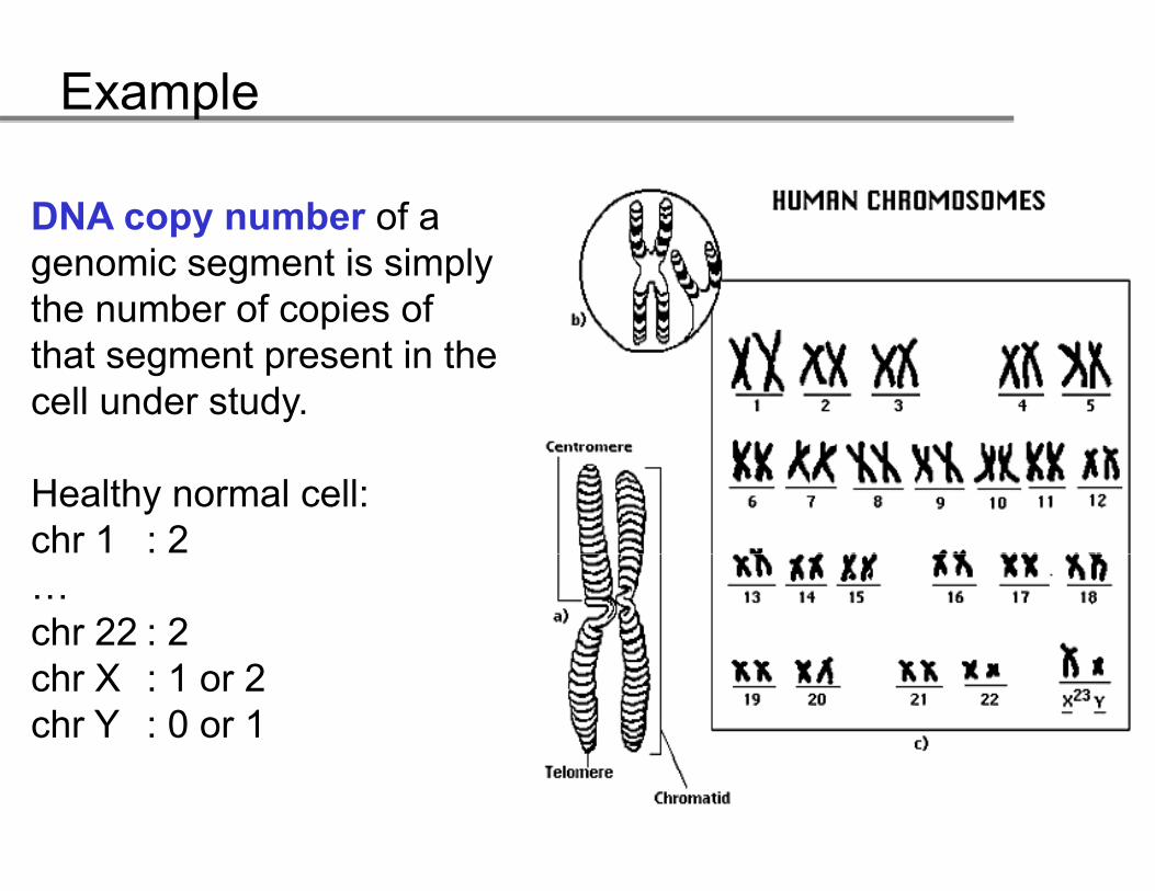
DNA copy number of a DNA copy number of a genomic segment is simply the number of copies of that segment present in the cell under study.
Healthy normal cell:chr 1 : 2…chr 22 : 2chr X : 1 or 2chr Y : 0 or 1
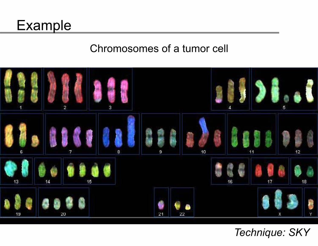
ExampleChromosomes of a tumor cell
Technique: SKY
Example
The DNA copy number is often categorized into:L l 2 i• L : loss : < 2 copies
• N : normal : 2 copies• G : gain : > 2 copies• G : gain : > 2 copies
In cancer:In cancer:• The number of DNA copy number aberrations
accumulates with the progression of the disease.p g• DNA copy number aberrations are believed to be
irreversible.
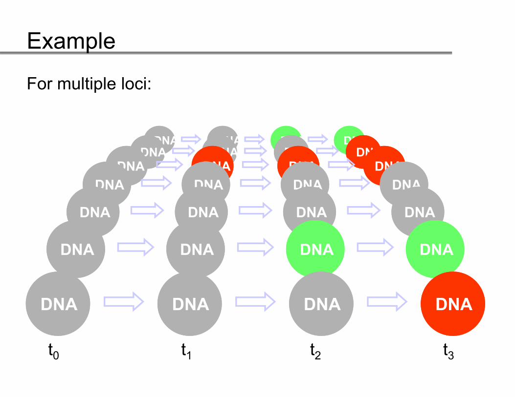
Let us model the accumulation process of DNA copy number aberrationsnumber aberrations.
Example
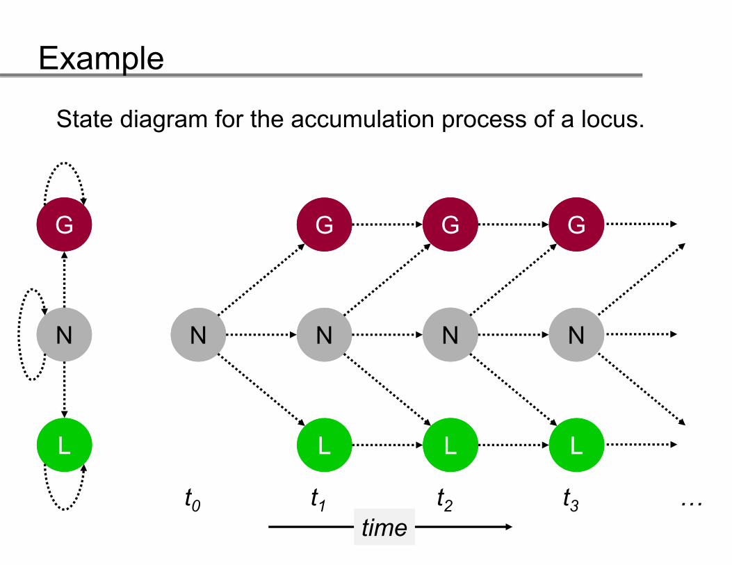
State diagram for the accumulation process of a locus.
GG GG GG GG
NN NN NN NN NN
LL
t
LL
t
LL
t
LL
tt0 t1 t2 t3 …time
Example
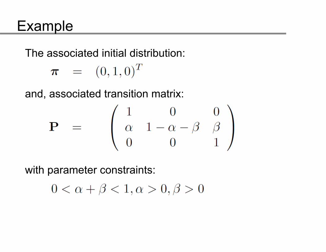
The associated initial distribution:
and associated transition matrix:and, associated transition matrix:
with parameter constraints:
Example
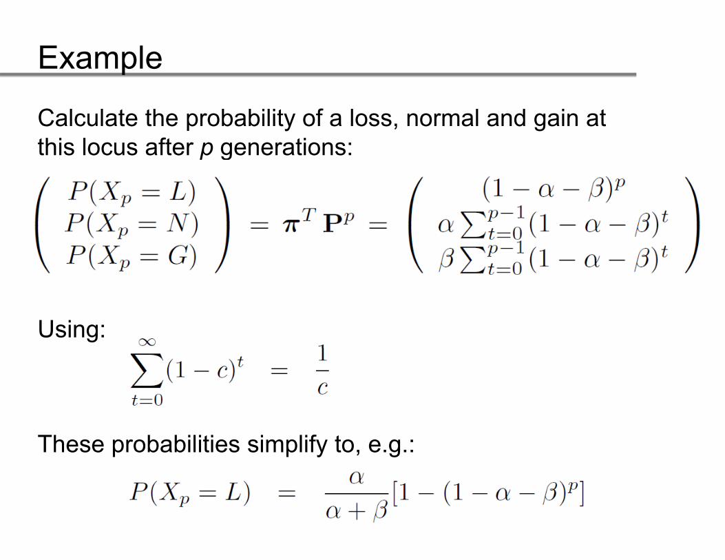
Calculate the probability of a loss, normal and gain at this locus after p generations:this locus after p generations:
Using:
These probabilities simplify to, e.g.:
Example
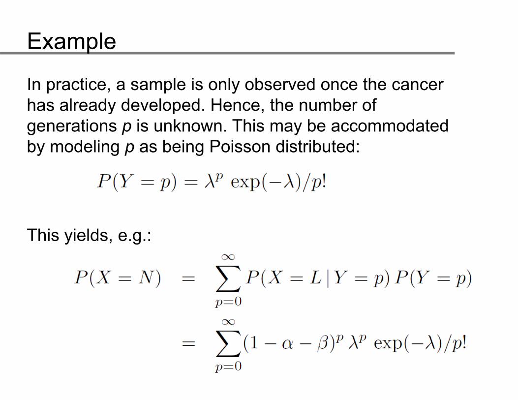
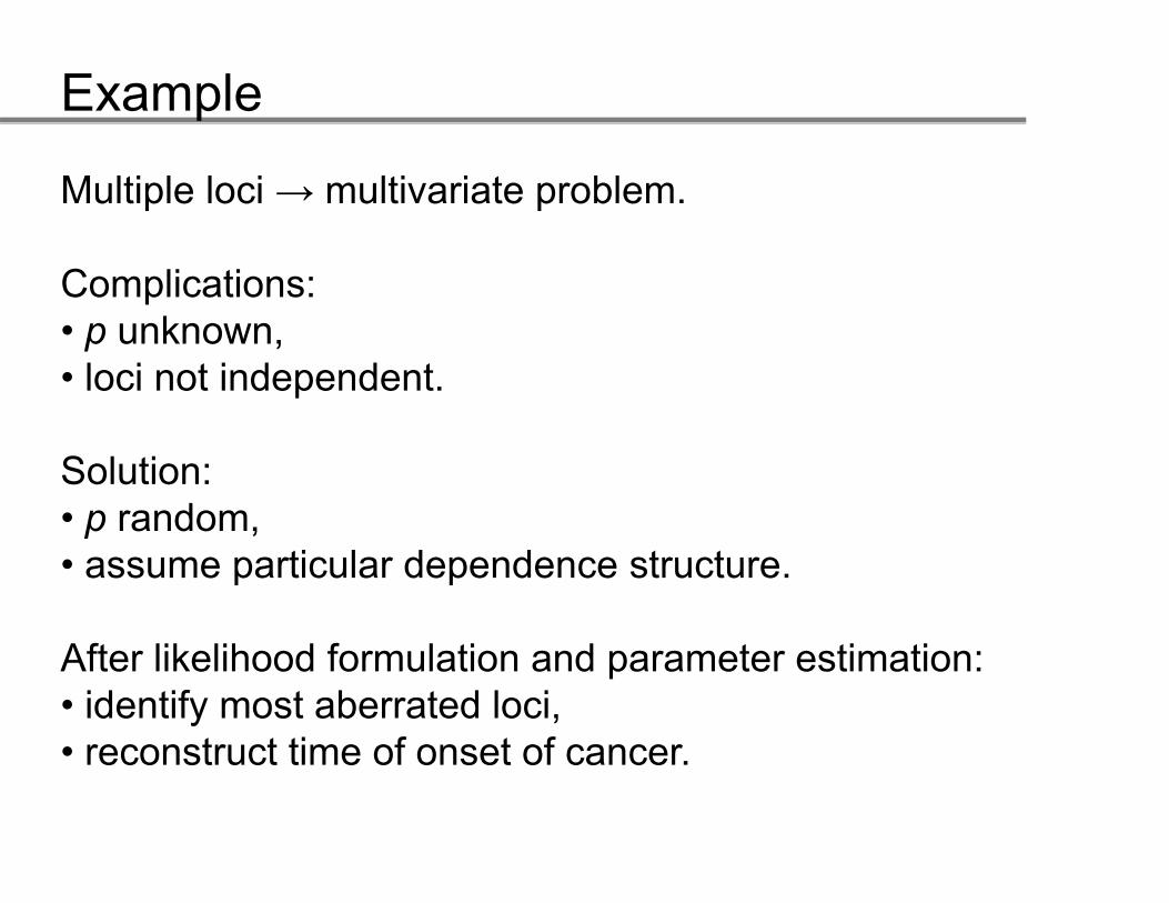
In practice, a sample is only observed once the cancer has already developed Hence the number ofhas already developed. Hence, the number of generations p is unknown. This may be accommodated by modeling p as being Poisson distributed:by modeling p as being Poisson distributed:
After likelihood formulation and parameter estimation:After likelihood formulation and parameter estimation: • identify most aberrated loci,• reconstruct time of onset of cancer.
Stationary distribution
Stationary distribution
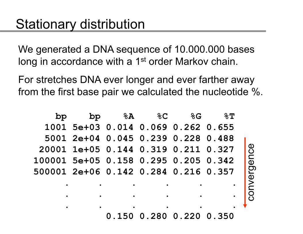
We generated a DNA sequence of 10.000.000 bases long in accordance with a 1st order Markov chainlong in accordance with a 1st order Markov chain.
For stretches DNA ever longer and ever farther away f th fi t b i l l t d th l tid %
bp bp %A %C %G %T
from the first base pair we calculated the nucleotide %.
bp bp %A %C %G %T 1001 5e+03 0.014 0.069 0.262 0.6555001 2e+04 0.045 0.239 0.228 0.488
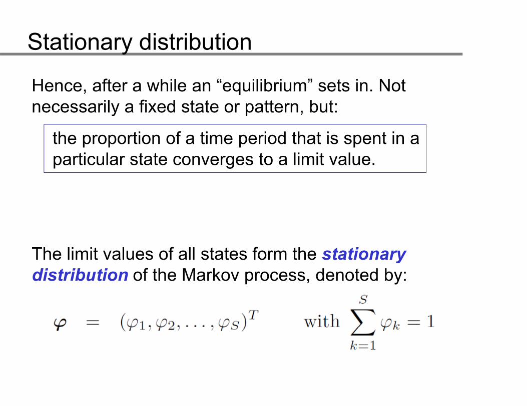
Hence, after a while an “equilibrium” sets in. Not necessarily a fixed state or pattern but:necessarily a fixed state or pattern, but:
the proportion of a time period that is spent in a ti l t t t li it lparticular state converges to a limit value.
The limit values of all states form the stationaryThe limit values of all states form the stationary distribution of the Markov process, denoted by:
Stationary distribution
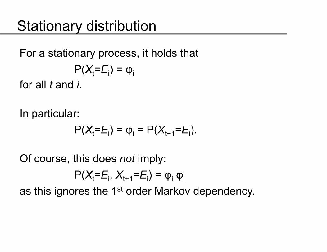
For a stationary process, it holds that P(Xt=Ei) = φi
for all t and i.
In particular: P(X E ) P(X E )P(Xt=Ei) = φi = P(Xt+1=Ei).
Of course this does not imply:Of course, this does not imply:P(Xt=Ei, Xt+1=Ei) = φi φi
thi i th 1 t d M k d das this ignores the 1st order Markov dependency.
Stationary distribution
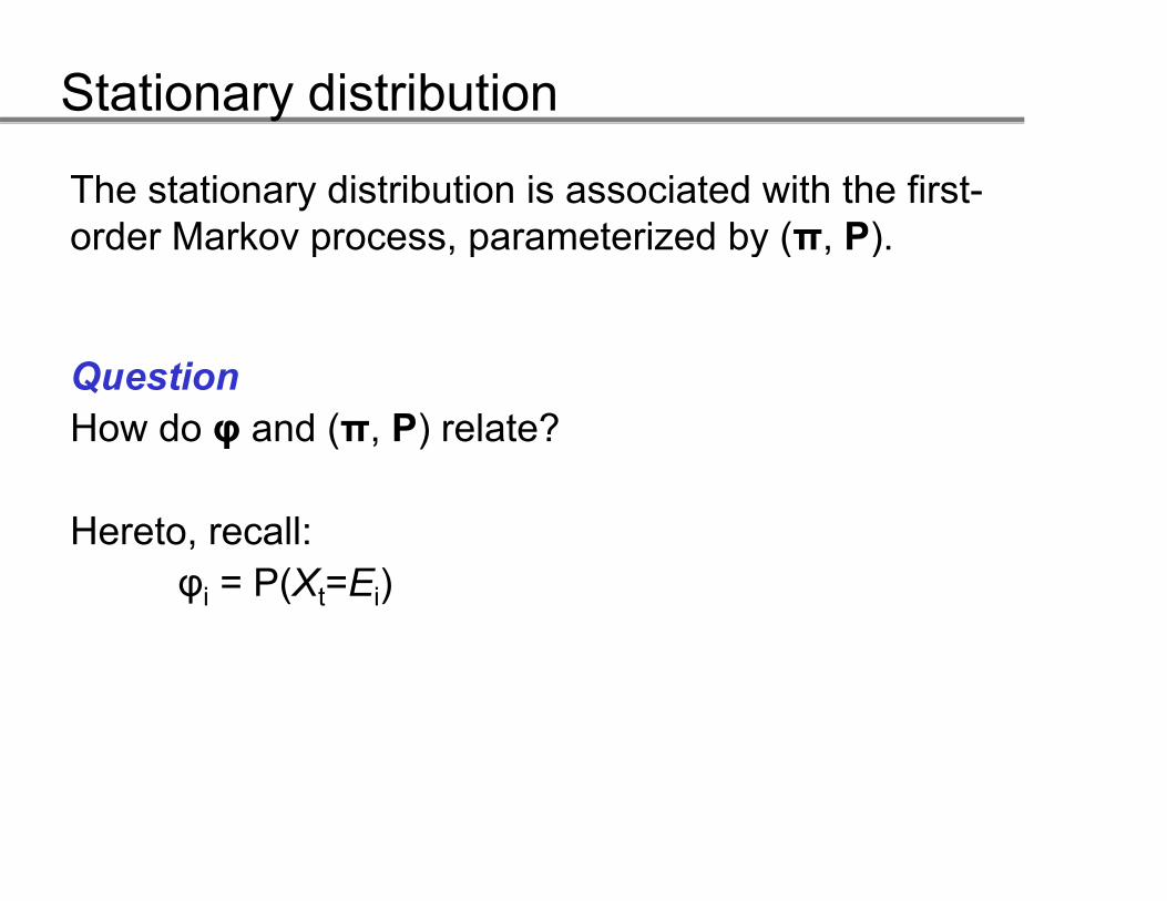
The stationary distribution is associated with the first-order Markov process parameterized by (π P)order Markov process, parameterized by (π, P).
QuestionHow do φ and (π, P) relate?
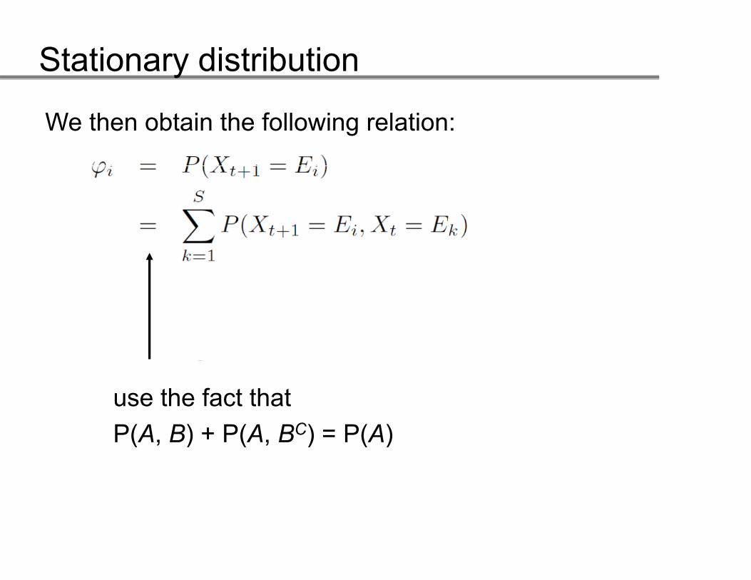
Hereto, recall:φi = P(Xt=Ei)
Stationary distribution
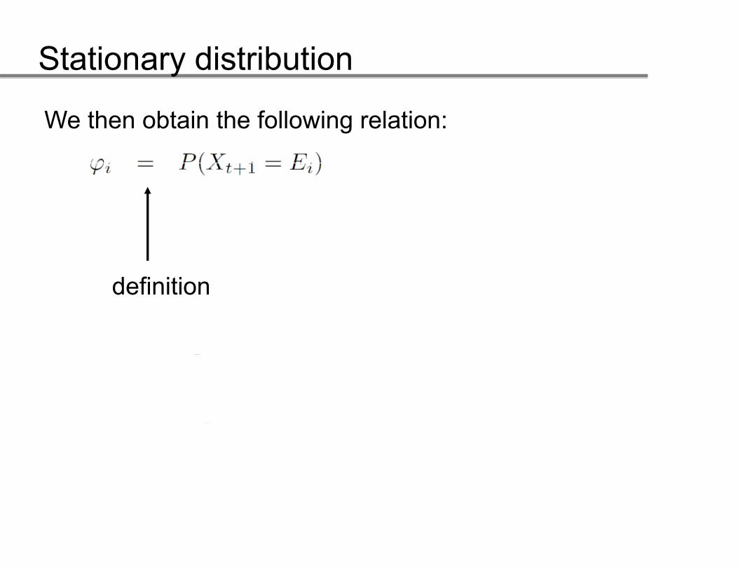
We then obtain the following relation:
definitiondefinition
Stationary distribution
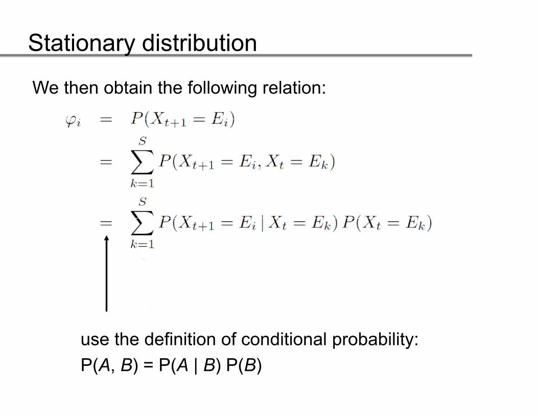
We then obtain the following relation:
use the fact thatP(A B) + P(A BC) = P(A)P(A, B) + P(A, BC) = P(A)
Stationary distribution
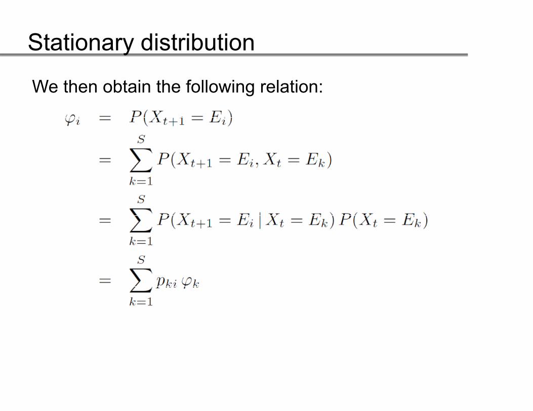
We then obtain the following relation:
use the definition of conditional probability:P(A B) P(A | B) P(B)P(A, B) = P(A | B) P(B)
Stationary distribution
We then obtain the following relation:
Stationary distribution
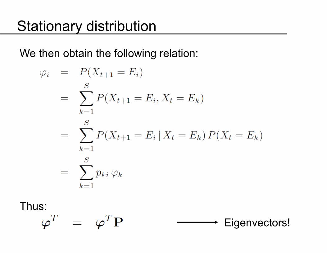
We then obtain the following relation:
Thus:Ei t !Eigenvectors!
Stationary distribution
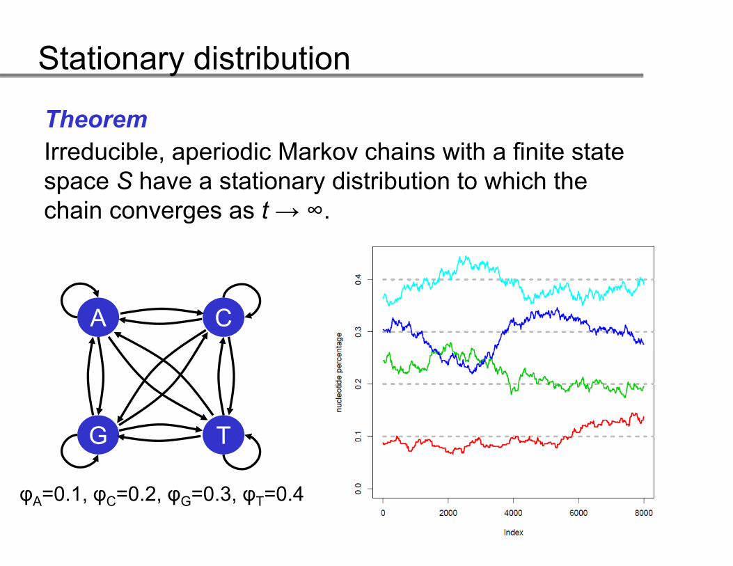
TheoremI d ibl i di M k h i ith fi it t tIrreducible, aperiodic Markov chains with a finite state space S have a stationary distribution to which the chain converges as t → ∞chain converges as t → .
A C
G T
0 1 0 2 0 3 0 4φA=0.1, φC=0.2, φG=0.3, φT=0.4
Stationary distribution
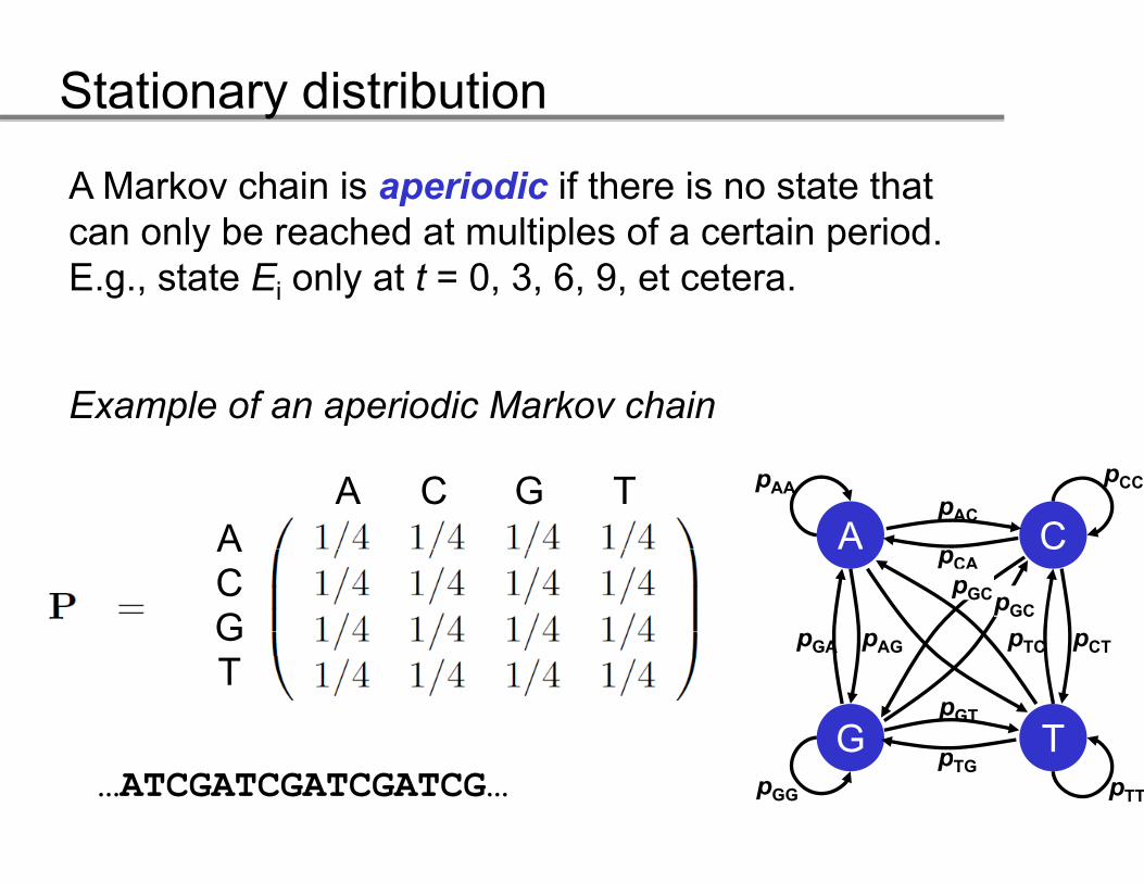
A Markov chain is aperiodic if there is no state that can only be reached at multiples of a certain periodcan only be reached at multiples of a certain period. E.g., state Ei only at t = 0, 3, 6, 9, et cetera.
Example of an aperiodic Markov chain
A C G TA A C
pCCpAApAC
ACG
A CpCA
pTC pCTpGA pAG
pGCpGC
T
G TpGT
pTG…ATCGATCGATCGATCG… pTTpGG
pTG
Stationary distribution
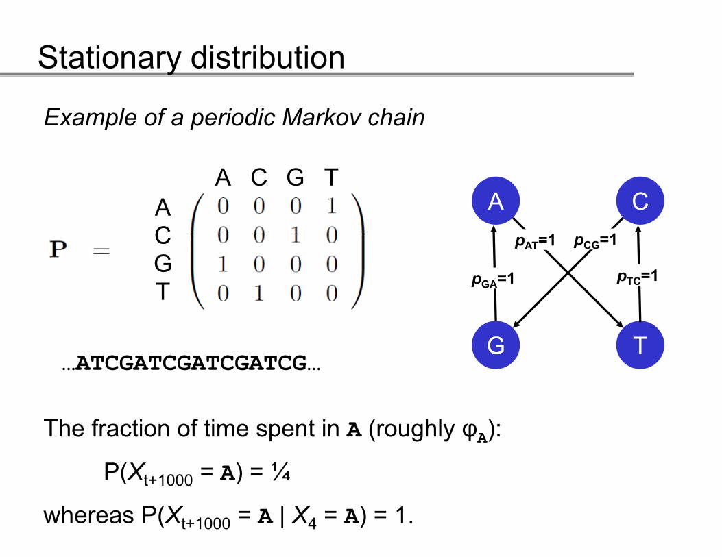
Example of a periodic Markov chain
A CA C G T
ApAT=1
pTC=1p =1
pCG=1
ACG
G T
pTC 1pGA=1T
G T…ATCGATCGATCGATCG…
The fraction of time spent in A (roughly φA):
P(Xt+1000 = A) = ¼ ( t+1000 )
whereas P(Xt+1000 = A | X4 = A) = 1.
Stationary distribution
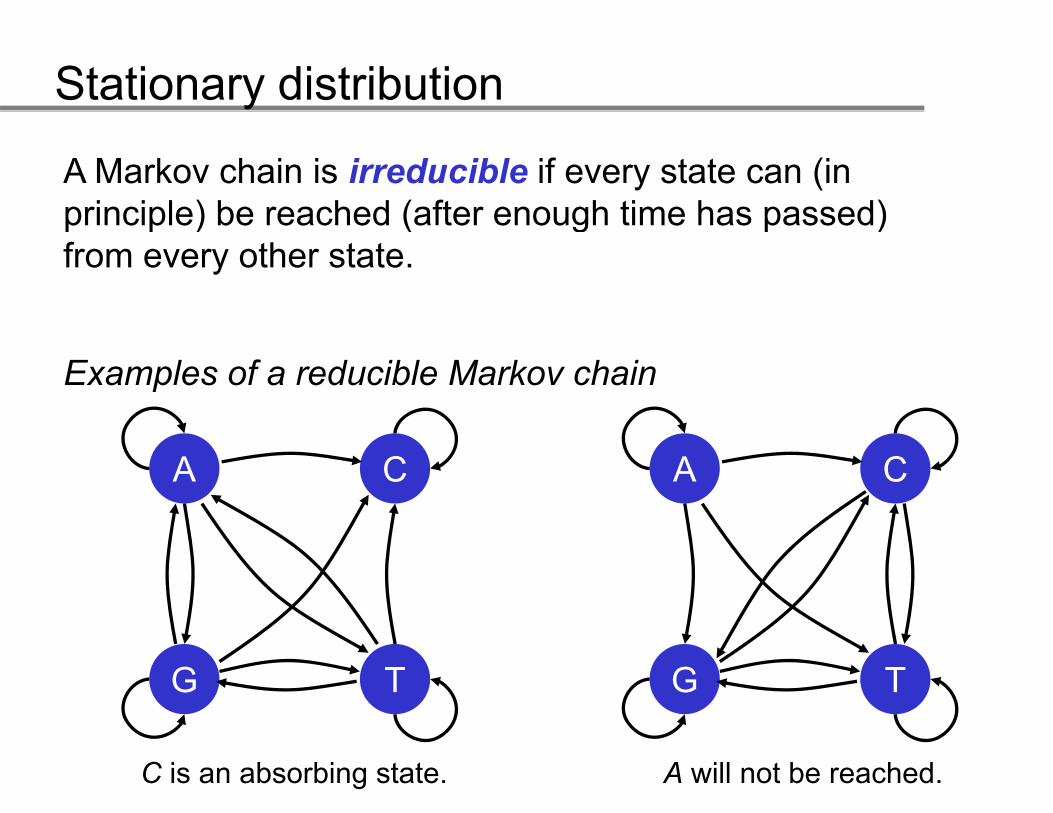
A Markov chain is irreducible if every state can (in principle) be reached (after enough time has passed)principle) be reached (after enough time has passed) from every other state.
Examples of a reducible Markov chain
A CA C
G TG T
C is an absorbing state. A will not be reached.
Stationary distribution
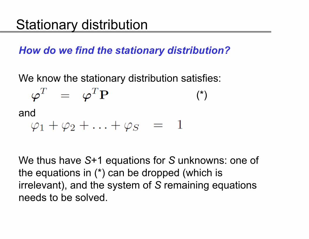
How do we find the stationary distribution?
We know the stationary distribution satisfies:
and
(*)
We thus have S+1 equations for S unknowns: one of the equations in (*) can be dropped (which is q ( ) pp (irrelevant), and the system of S remaining equations needs to be solved.
Stationary distribution
Consider the transition matrix:
In order to find the stationary distribution we need toIn order to find the stationary distribution we need to solve the following system of equations:
This yields: (φ1, φ2)T = (0.5547945, 0.4452055)T
Stationary distribution
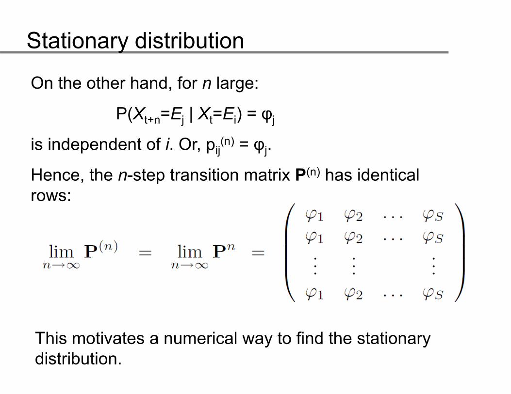
On the other hand, for n large:
P(Xt+n=Ej | Xt=Ei) = φj
is independent of i. Or, pij(n) = φj.is independent of i. Or, pij φj.
Hence, the n-step transition matrix P(n) has identical rows:rows:
This motivates a numerical way to find the stationaryThis motivates a numerical way to find the stationary distribution.
Stationary distribution
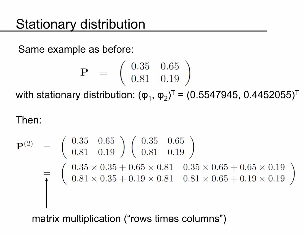
Same example as before:
Th
with stationary distribution: (φ1, φ2)T = (0.5547945, 0.4452055)T
Then:
matrix multiplication (“rows times columns”)
Stationary distribution
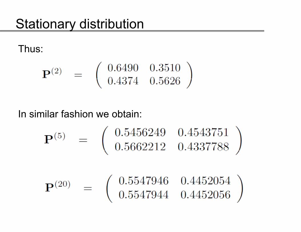
Thus:
In similar fashion we obtain:In similar fashion we obtain:
Convergence of theConvergence of the stationary distributionstationary distribution
Convergence to the stationary distribution
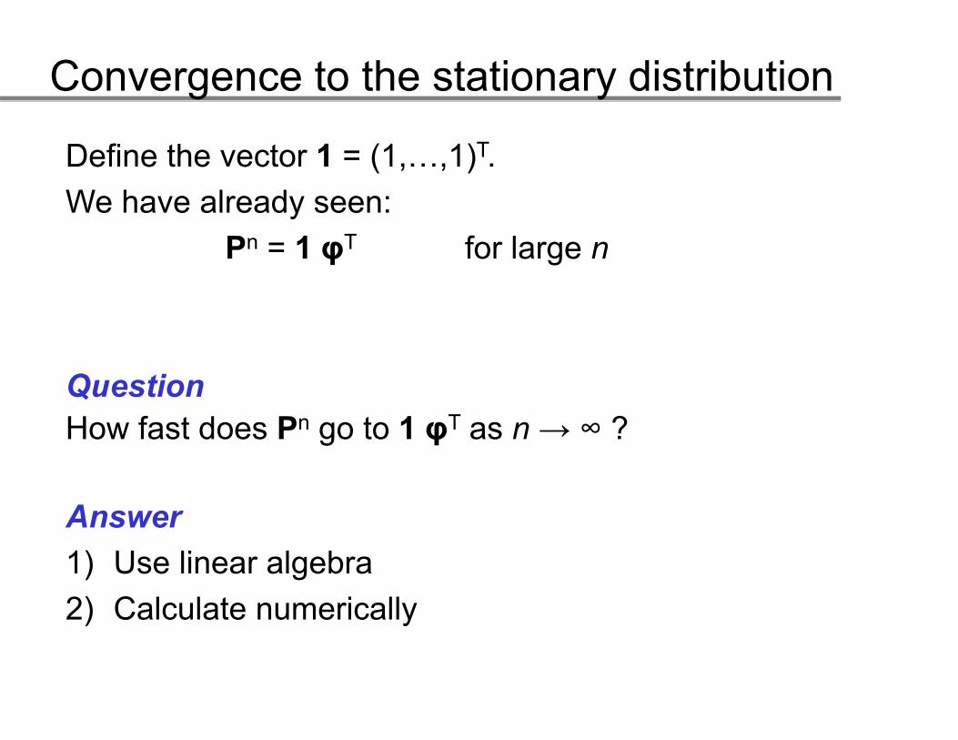
Define the vector 1 = (1,…,1)T.W h l dWe have already seen:
Pn = 1 φT for large n
QuestionHow fast does Pn go to 1 φT as n → ∞ ?
Answer1) Use linear algebra2) Calculate numerically
Convergence to the stationary distribution
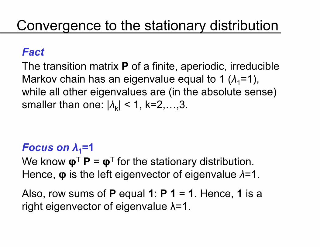
FactTh t iti t i P f fi it i di i d iblThe transition matrix P of a finite, aperiodic, irreducible Markov chain has an eigenvalue equal to 1 (λ1=1), while all other eigenvalues are (in the absolute sense)while all other eigenvalues are (in the absolute sense) smaller than one: |λk| < 1, k=2,…,3.
Focus on λ1=11We know φT P = φT for the stationary distribution. Hence, φ is the left eigenvector of eigenvalue λ=1.
Also, row sums of P equal 1: P 1 = 1. Hence, 1 is a right eigenvector of eigenvalue λ=1.
Convergence to the stationary distribution
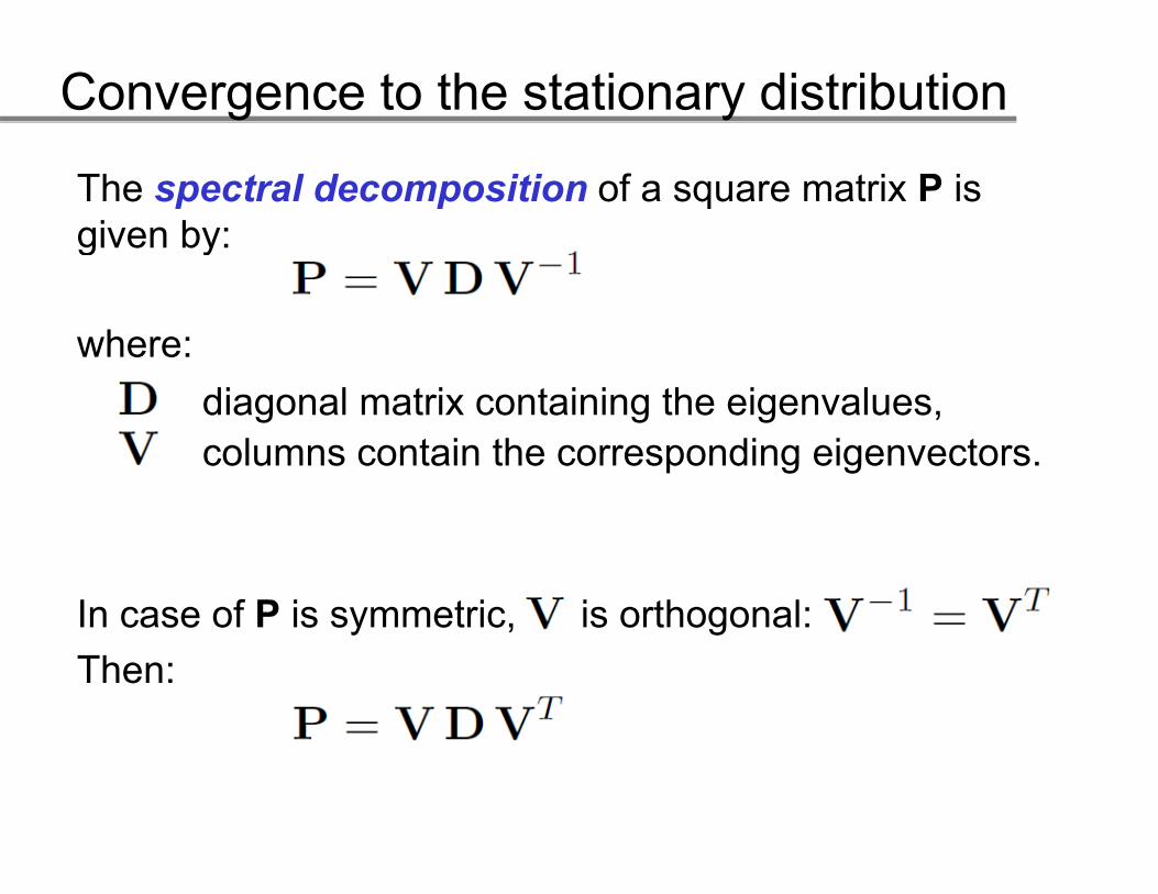
The spectral decomposition of a square matrix P is given by:given by:
where:where:diagonal matrix containing the eigenvalues,columns contain the corresponding eigenvectorscolumns contain the corresponding eigenvectors.
In case of P is symmetric, is orthogonal: Then:Then:
Convergence to the stationary distribution
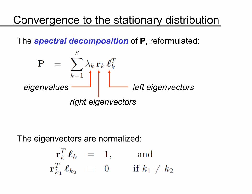
The spectral decomposition of P, reformulated:
eigenvalues left eigenvectors
right eigenvectors
The eigenvectors are normalized:
Convergence to the stationary distribution
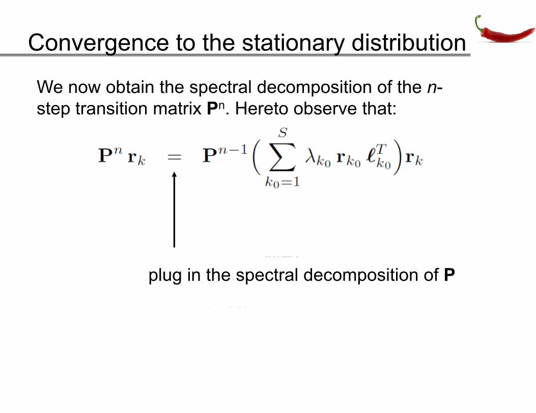
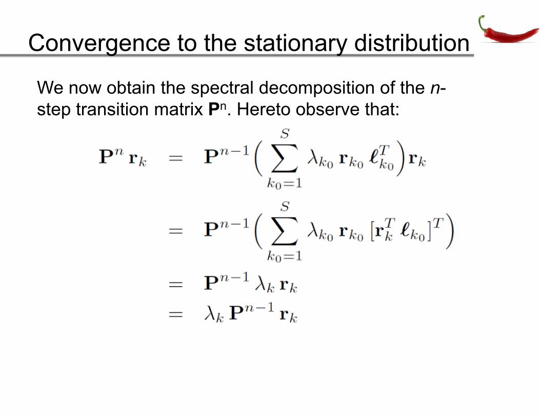
We now obtain the spectral decomposition of the n-step transition matrix Pn Hereto observe that:step transition matrix Pn. Hereto observe that:
plug in the spectral decomposition of P
Convergence to the stationary distribution
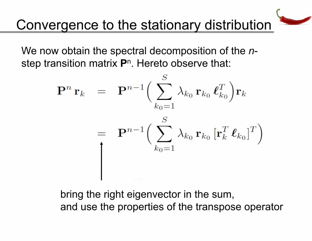
We now obtain the spectral decomposition of the n-step transition matrix Pn Hereto observe that:step transition matrix Pn. Hereto observe that:
bring the right eigenvector in the sum,and use the properties of the transpose operatorand use the properties of the transpose operator
Convergence to the stationary distribution
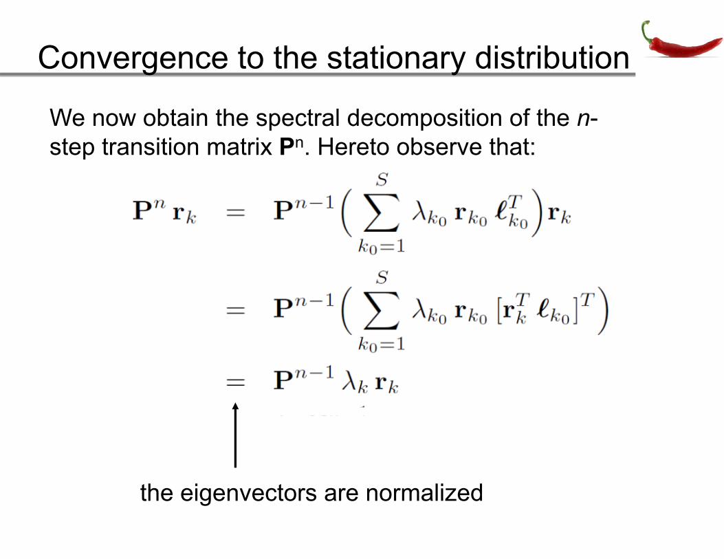
We now obtain the spectral decomposition of the n-step transition matrix Pn Hereto observe that:step transition matrix Pn. Hereto observe that:
the eigenvectors are normalized
Convergence to the stationary distribution
We now obtain the spectral decomposition of the n-step transition matrix Pn Hereto observe that:step transition matrix Pn. Hereto observe that:
Convergence to the stationary distribution
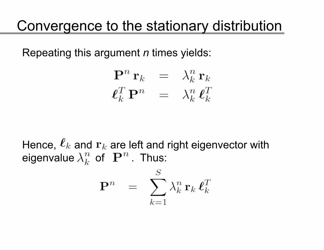
Repeating this argument n times yields:
Hence, and are left and right eigenvector with i l f Theigenvalue of . Thus:
Convergence to the stationary distribution
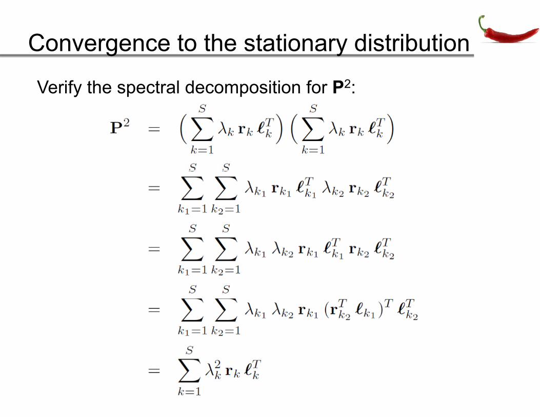
Verify the spectral decomposition for P2:
Convergence to the stationary distribution
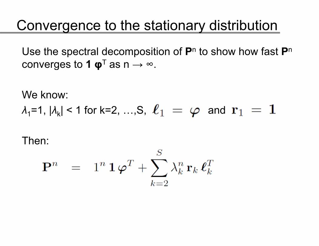
Use the spectral decomposition of Pn to show how fast Pn
converges to 1 φT as n → ∞converges to 1 φT as n → ∞.
We know:We know:λ1=1, |λk| < 1 for k=2, …,S, and
Then:
Convergence to the stationary distribution
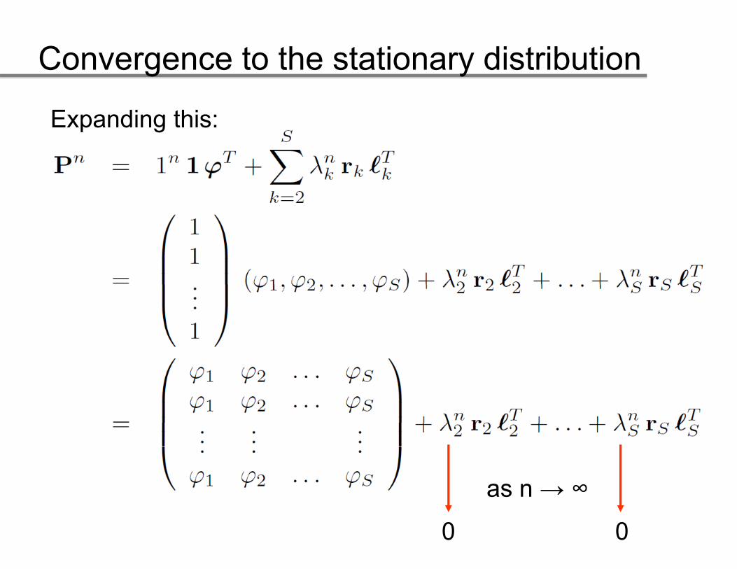
Expanding this:
as n → ∞
0 0
as n → ∞
Convergence to the stationary distribution
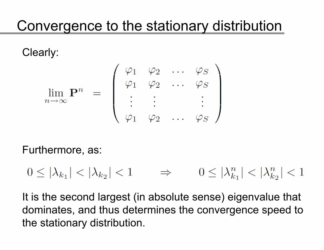
Clearly:
Furthermore, as:
It is the second largest (in absolute sense) eigenvalue that dominates, and thus determines the convergence speed to the stationary distribution.
Convergence to the stationary distribution
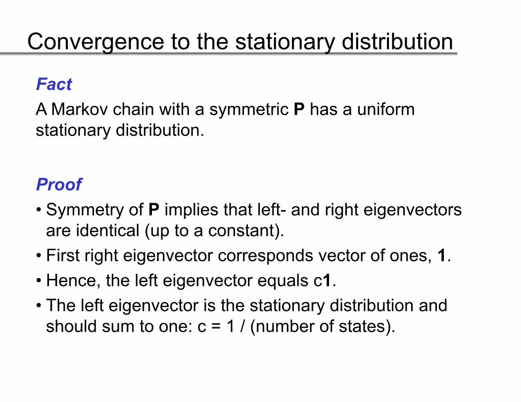
FactA M k h i ith t i P h ifA Markov chain with a symmetric P has a uniform stationary distribution.
Proof• Symmetry of P implies that left- and right eigenvectors
are identical (up to a constant). Fi t i ht i t d t f 1• First right eigenvector corresponds vector of ones, 1.
• Hence, the left eigenvector equals c1.Th l f i i h i di ib i d• The left eigenvector is the stationary distribution and should sum to one: c = 1 / (number of states).
Convergence to the stationary distribution
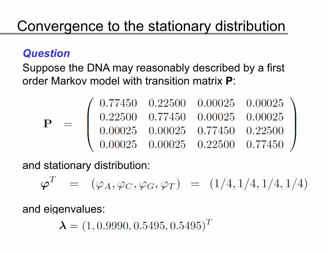
QuestionS th DNA bl d ib d b fi tSuppose the DNA may reasonably described by a first order Markov model with transition matrix P:
and stationary distribution:
and eigenvalues:
Convergence to the stationary distribution
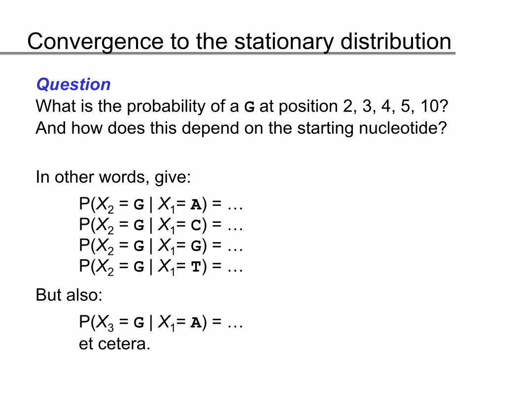
QuestionWhat is the probability of a G at position 2 3 4 5 10?What is the probability of a G at position 2, 3, 4, 5, 10? And how does this depend on the starting nucleotide?
In other words, give:P(X G | X A)P(X2 = G | X1= A) = …P(X2 = G | X1= C) = …P(X2 = G | X1= G) =P(X2 G | X1 G) …P(X2 = G | X1= T) = …
But also:But also:P(X3 = G | X1= A) = …et ceteraet cetera.
Convergence to the stationary distribution
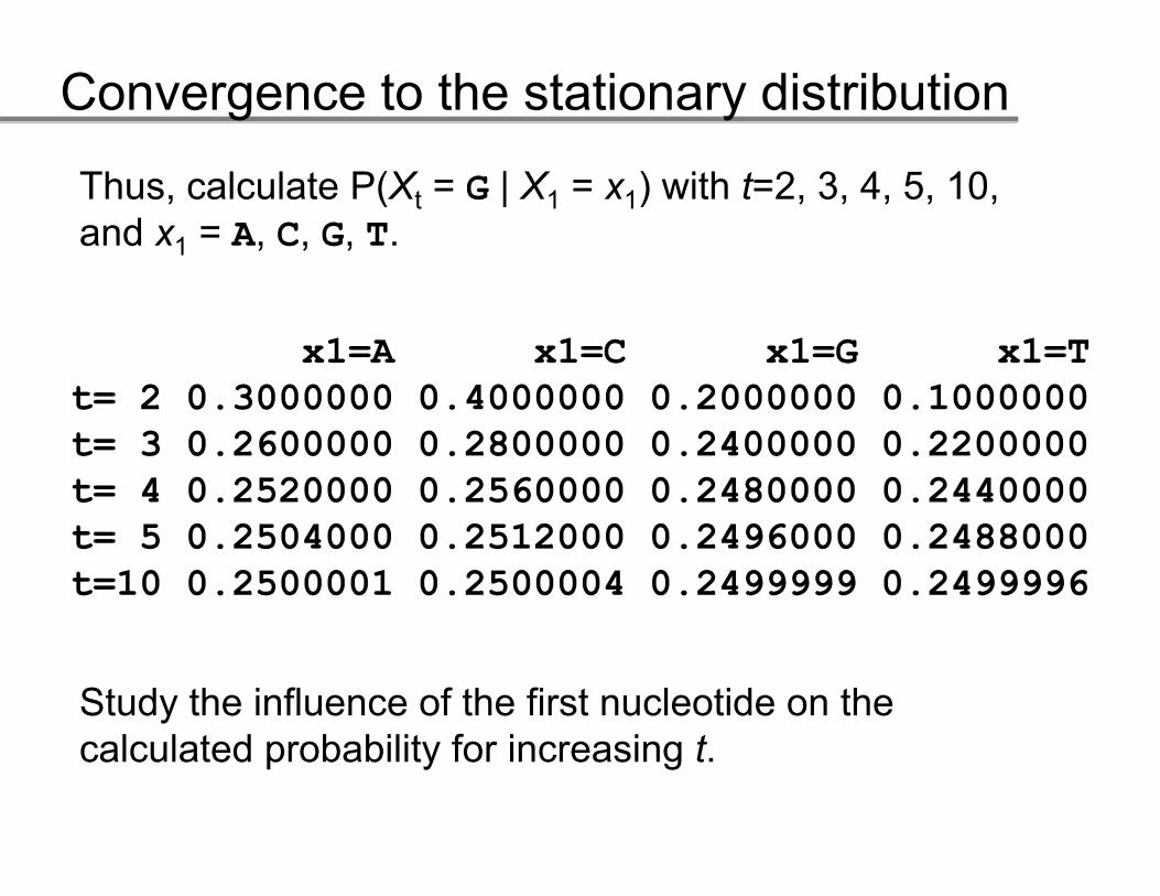
Thus, calculate P(Xt = G | X1 = x1) with t=2, 3, 4, 5, 10, and x = A C G T
Study the influence of the first nucleotide on the calculated probability for increasing t.
Convergence to the stationary distribution
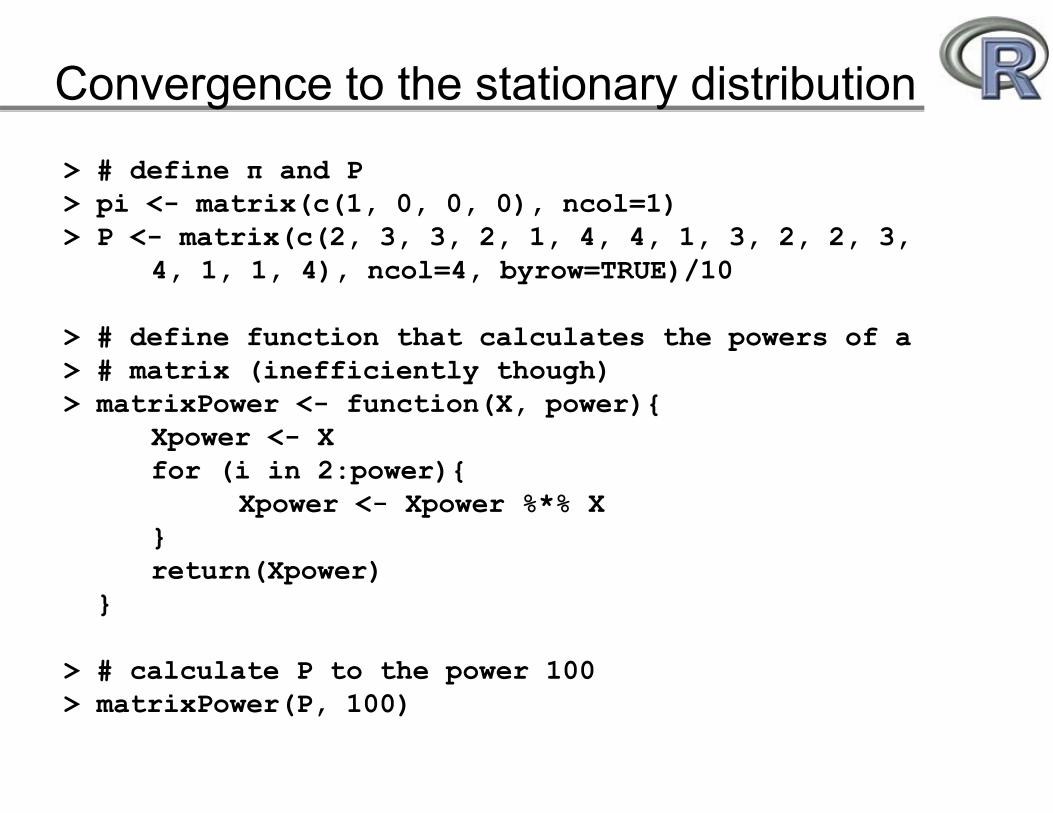
> # define π and P> pi <- matrix(c(1, 0, 0, 0), ncol=1)> pi < matrix(c(1, 0, 0, 0), ncol 1)> P <- matrix(c(2, 3, 3, 2, 1, 4, 4, 1, 3, 2, 2, 3,
4, 1, 1, 4), ncol=4, byrow=TRUE)/10
> # define function that calculates the powers of a > # matrix (inefficiently though)> matrixPower <- function(X power){> matrixPower < function(X, power){
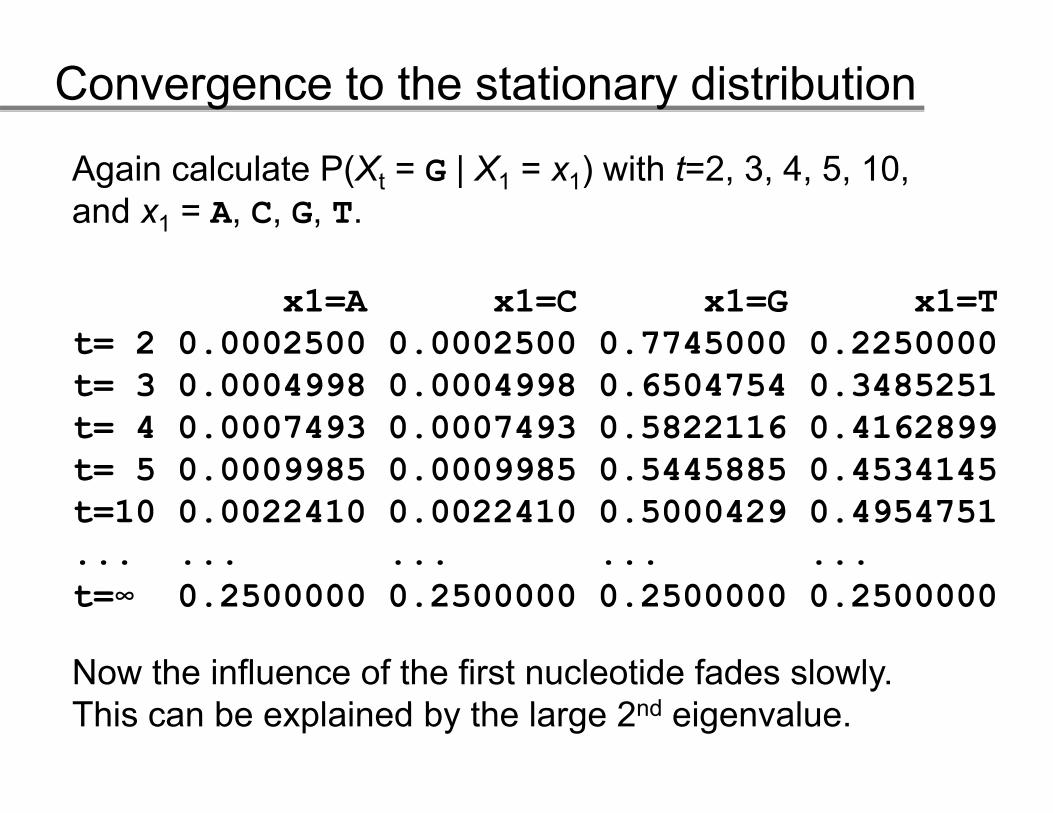
Now the influence of the first nucleotide fades slowly. Thi b l i d b th l 2 d i l
t 0.2500000 0.2500000 0.2500000 0.2500000
This can be explained by the large 2nd eigenvalue.
ProcessesProcesses back in timeback in time
Processes back in time
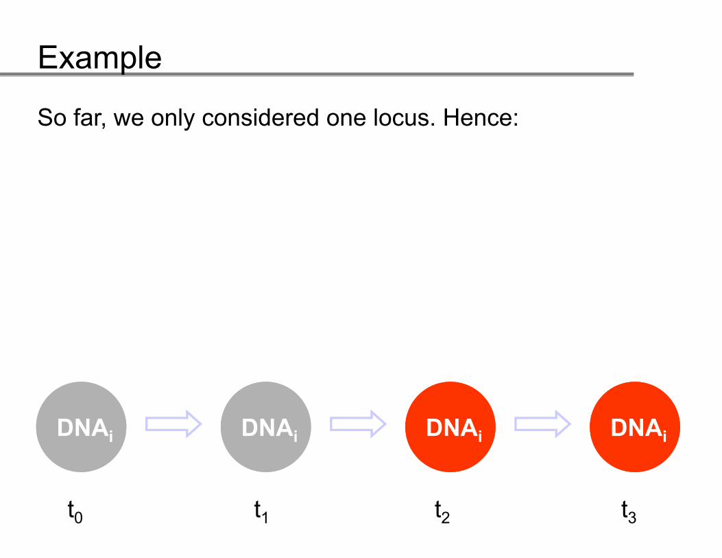
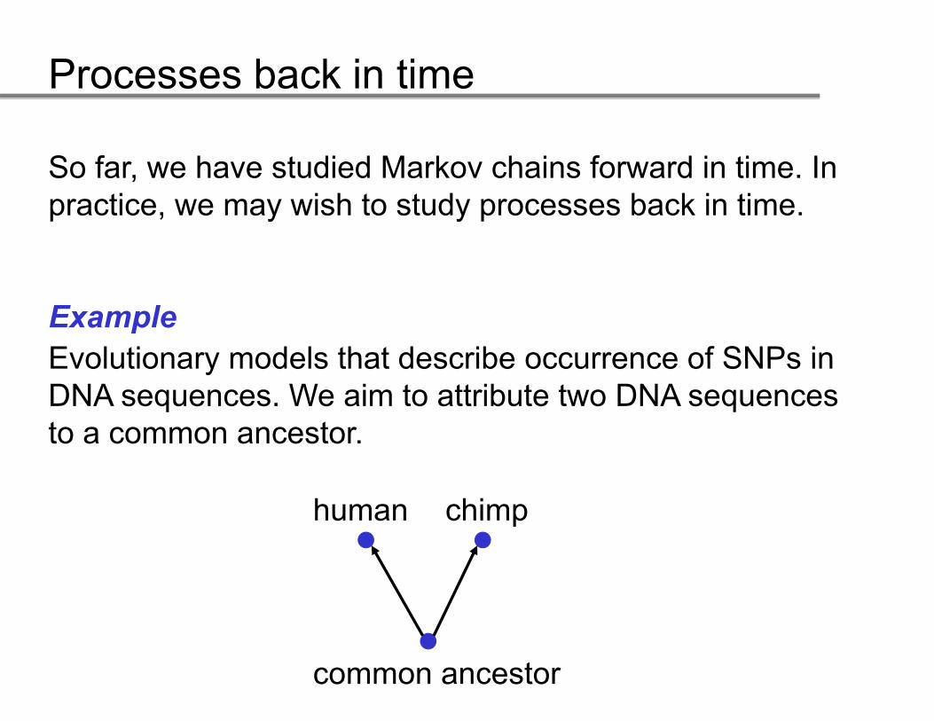
So far, we have studied Markov chains forward in time. In practice, we may wish to study processes back in time.
ExampleEvolutionary models that describe occurrence of SNPs inEvolutionary models that describe occurrence of SNPs in DNA sequences. We aim to attribute two DNA sequences to a common ancestor.
human chimp
common ancestor
Processes back in time
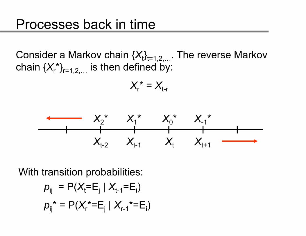
Consider a Markov chain {Xt}t=1,2,…. The reverse Markov t t , ,chain {Xr*}r=1,2,… is then defined by:
Xr* = Xt-rr t-r
X * X * X * X *
Xt-2 Xt-1 Xt Xt+1
X2 X1 X0 X-1
t 2 t 1 t t 1
With transition probabilities:With transition probabilities:pij = P(Xt=Ej | Xt-1=Ei)
p * = P(X *=E | X *=E )pij* = P(Xr*=Ej | Xr-1*=Ei)
Processes back in time
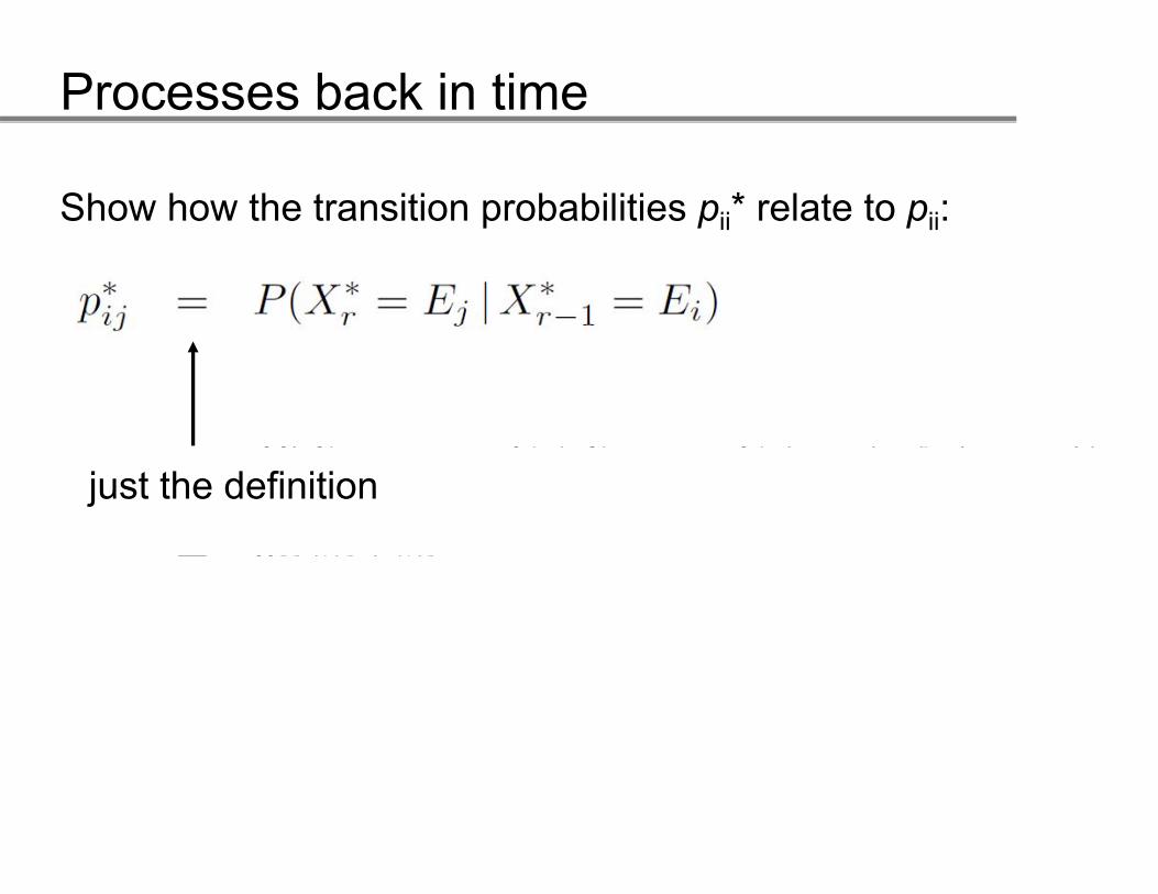
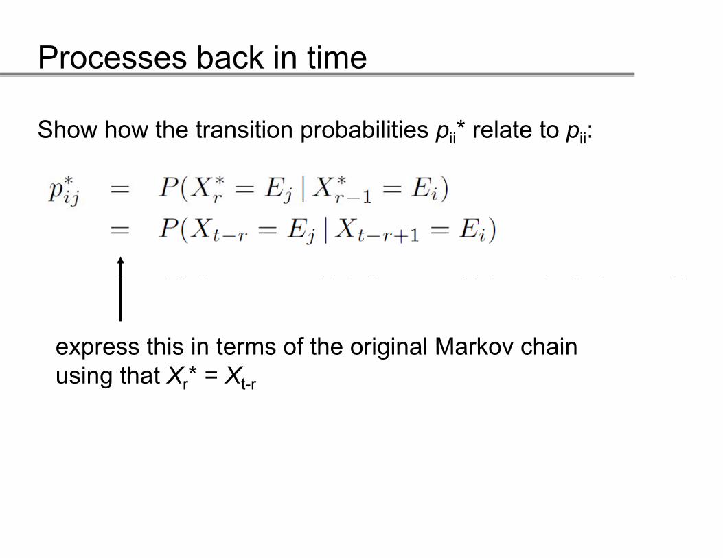
Show how the transition probabilities pji* relate to pij:
just the definition
Processes back in time
Show how the transition probabilities pji* relate to pij:
express this in terms of the original Markov chainexpress this in terms of the original Markov chain using that Xr* = Xt-r
Processes back in time
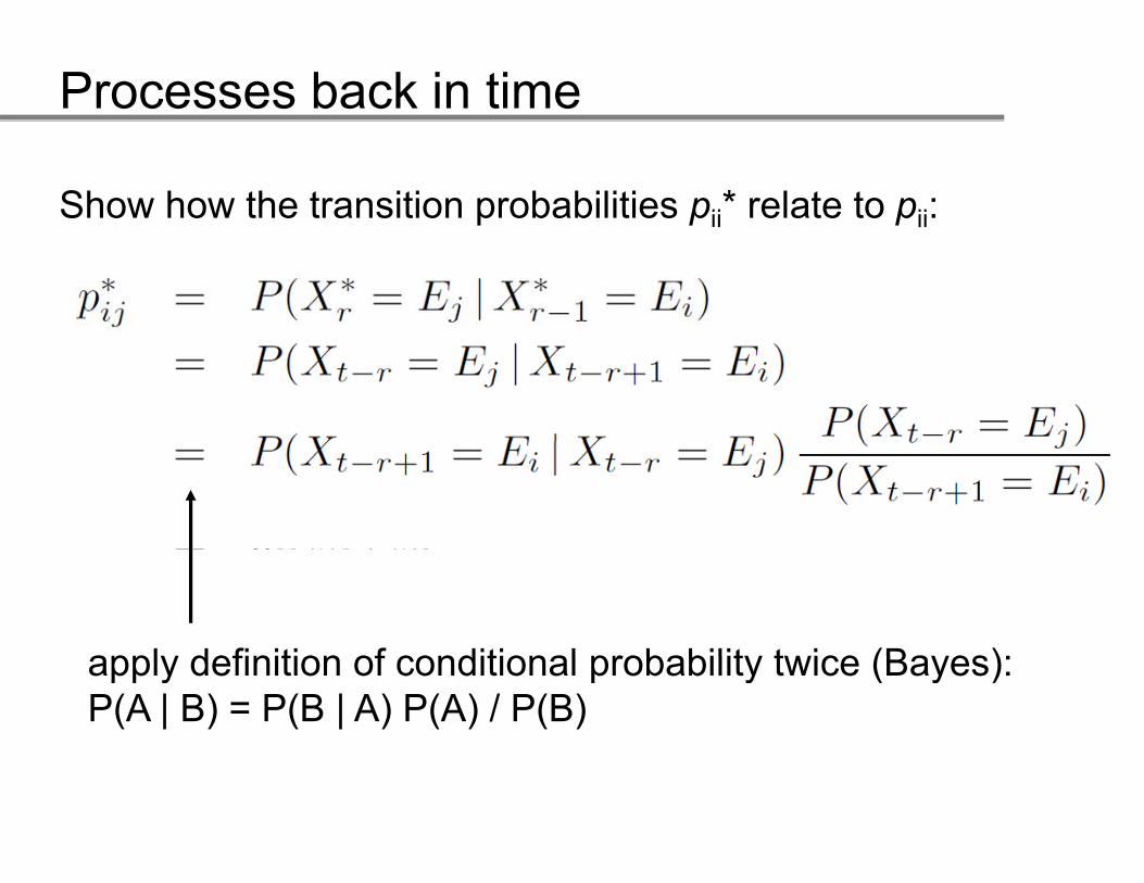
Show how the transition probabilities pji* relate to pij:
apply definition of conditional probability twice (Bayes):apply definition of conditional probability twice (Bayes):P(A | B) = P(B | A) P(A) / P(B)
Processes back in time
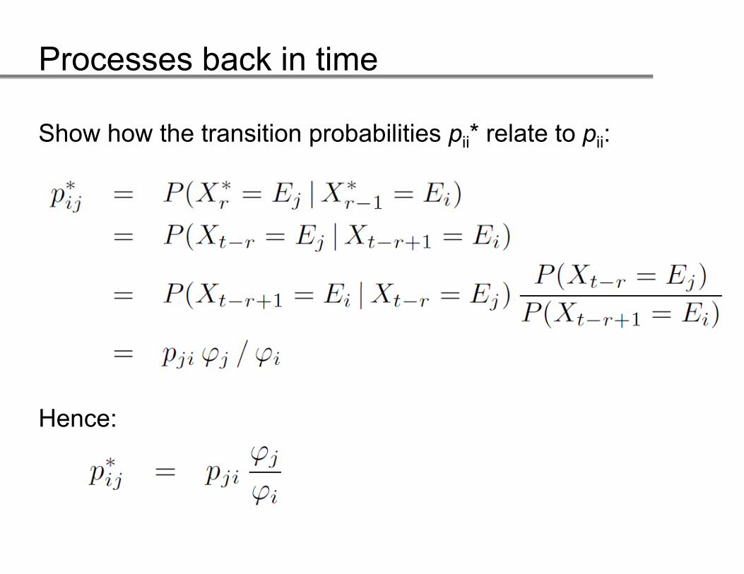
Show how the transition probabilities pji* relate to pij:
Hence:Hence:
Processes back in time
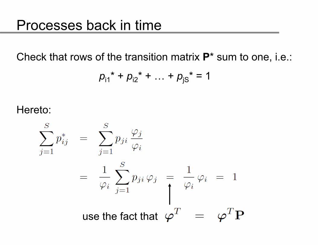
Check that rows of the transition matrix P* sum to one, i.e.:
pi1* + pi2* + … + pjS* = 1
Hereto:
use the fact that
Processes back in time
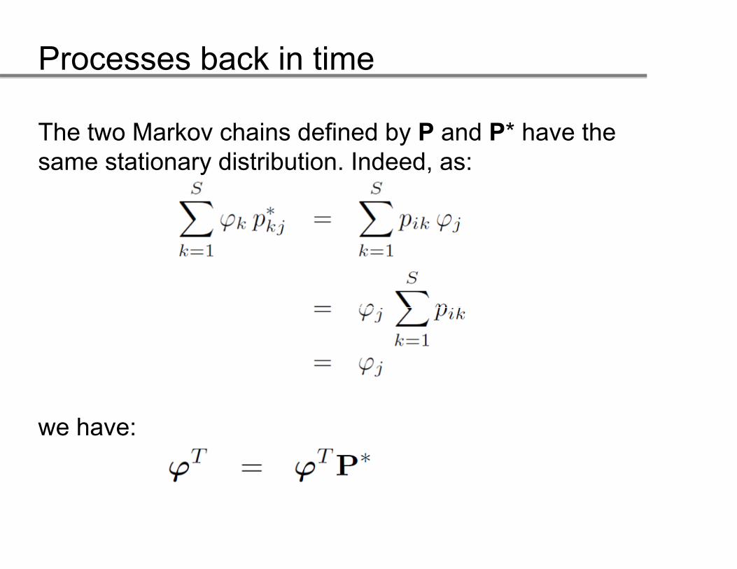
The two Markov chains defined by P and P* have the same stationary distribution. Indeed, as:
we have:we have:
Processes back in time
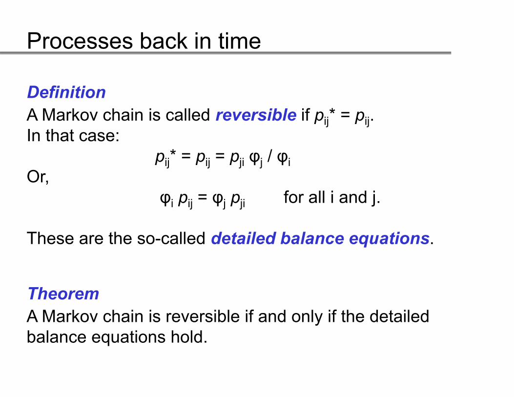
DefinitionA Markov chain is called reversible if pij* = pij. In that case:
* /pij* = pij = pji φj / φiOr,
φ p = φ p for all i and jφi pij = φj pji for all i and j.
These are the so-called detailed balance equations.q
TheoremTheoremA Markov chain is reversible if and only if the detailed balance equations hold.q
Processes back in time
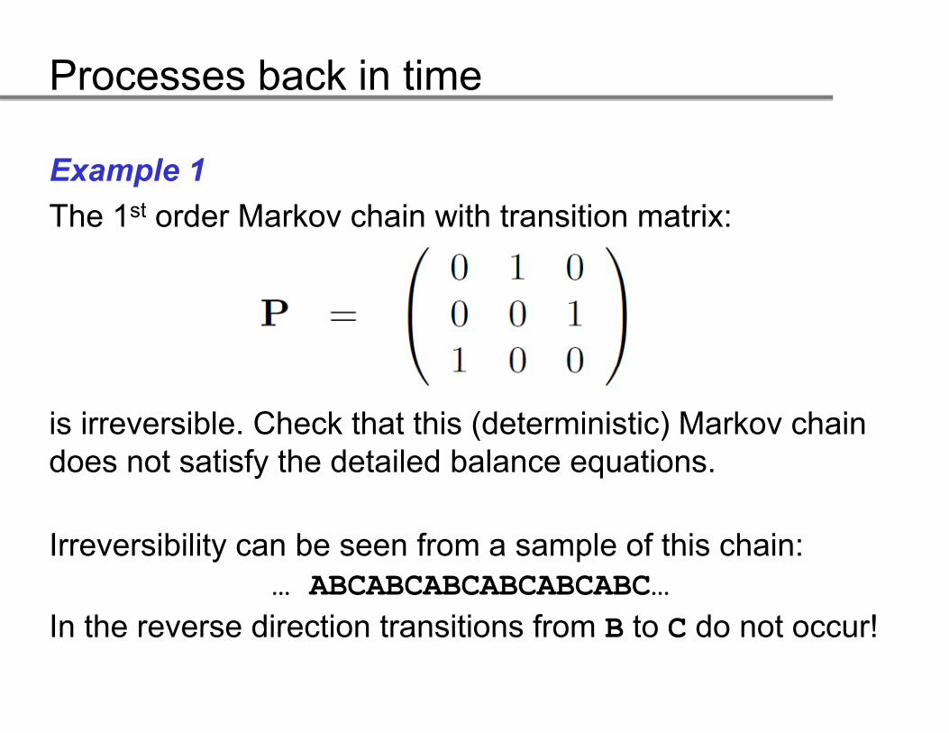
Example 1The 1st order Markov chain with transition matrix:
is irreversible. Check that this (deterministic) Markov chain does not satisfy the detailed balance equationsdoes not satisfy the detailed balance equations.
Irreversibility can be seen from a sample of this chain:Irreversibility can be seen from a sample of this chain:… ABCABCABCABCABCABC…
In the reverse direction transitions from B to C do not occur!In the reverse direction transitions from B to C do not occur!
Processes back in time
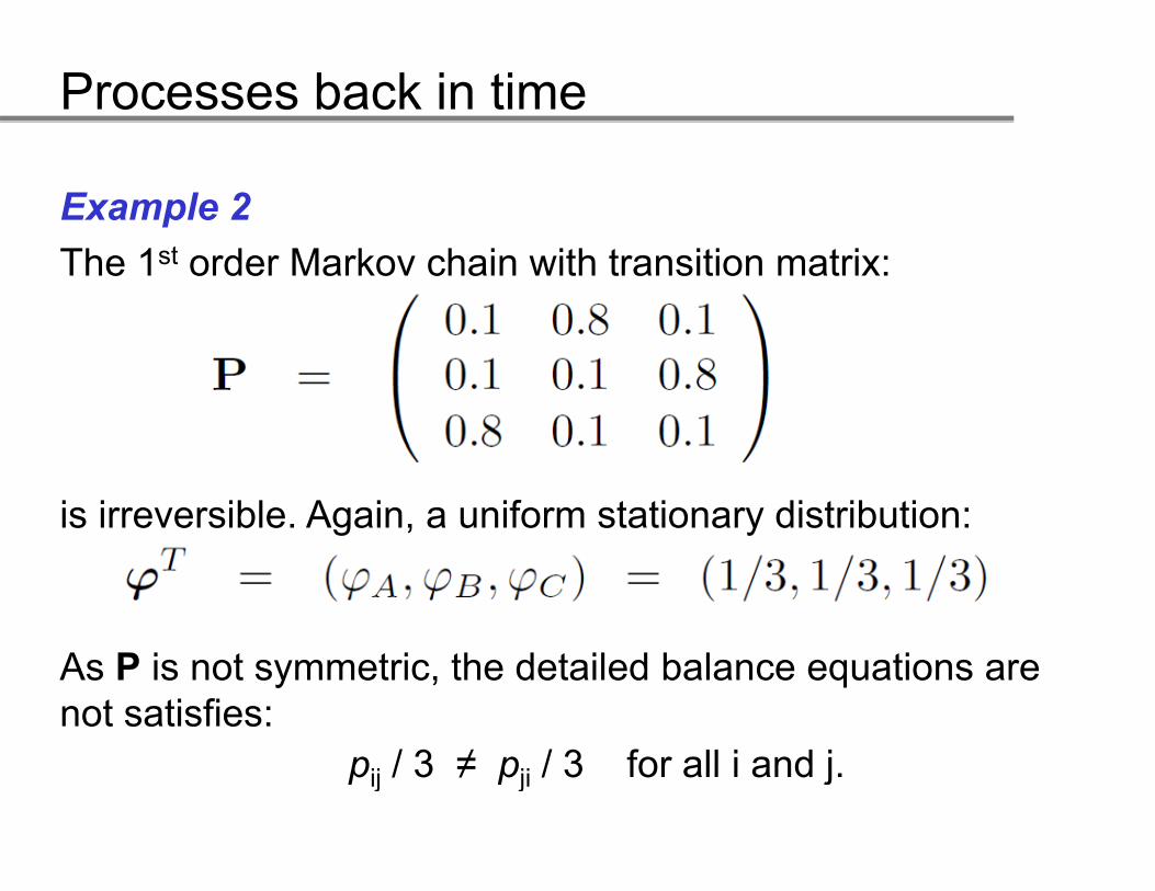
Example 2The 1st order Markov chain with transition matrix:
is irreversible. Again, a uniform stationary distribution:
As P is not symmetric the detailed balance equations areAs P is not symmetric, the detailed balance equations are not satisfies:
pij / 3 ≠ pji / 3 for all i and jpij / 3 ≠ pji / 3 for all i and j.
Processes back in time
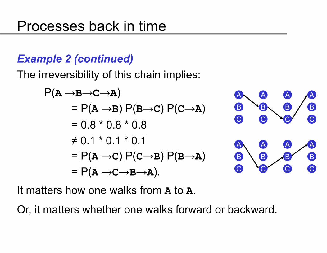
Example 2 (continued)The irreversibility of this chain implies:
P(A→B→C→A) A A A AP(A B C A) = P(A→B) P(B→C) P(C→A)= 0 8 * 0 8 * 0 8
Or, it matters whether one walks forward or backward.
Processes back in time
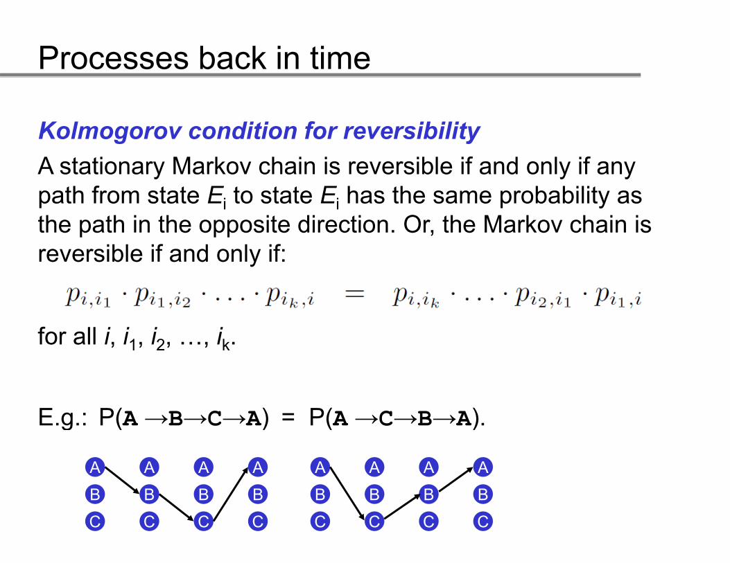
Kolmogorov condition for reversibilityA stationary Markov chain is reversible if and only if any path from state Ei to state Ei has the same probability as the path in the opposite direction. Or, the Markov chain is reversible if and only if:
for all i, i1, i2, …, ik.1 2 k
E g : P(A→B→C→A) = P(A→C→B→A)E.g.: P(A→B→C→A) = P(A→C→B→A).
A A A A A A A A
B
C
B
C
B
C
B
C
B
C
B
C
B
C
B
C
Processes back in time
InterpretationFor a reversible Markov chain it is not possible to determine the direction of the process from the observed state sequence alone.
M l l h l ti i t t t• Molecular phylogenetics aims to reconstruct evolutionary relationships between present day species from their DNA sequences Reversibility is then anfrom their DNA sequences. Reversibility is then an essential assumption.
• Genes are transcribed in one direction only (from the 3’• Genes are transcribed in one direction only (from the 3 end to the 5’ end). The promoter is only on the 3’ end. This suggests irreversibility. s suggests e e s b ty
Processes back in time
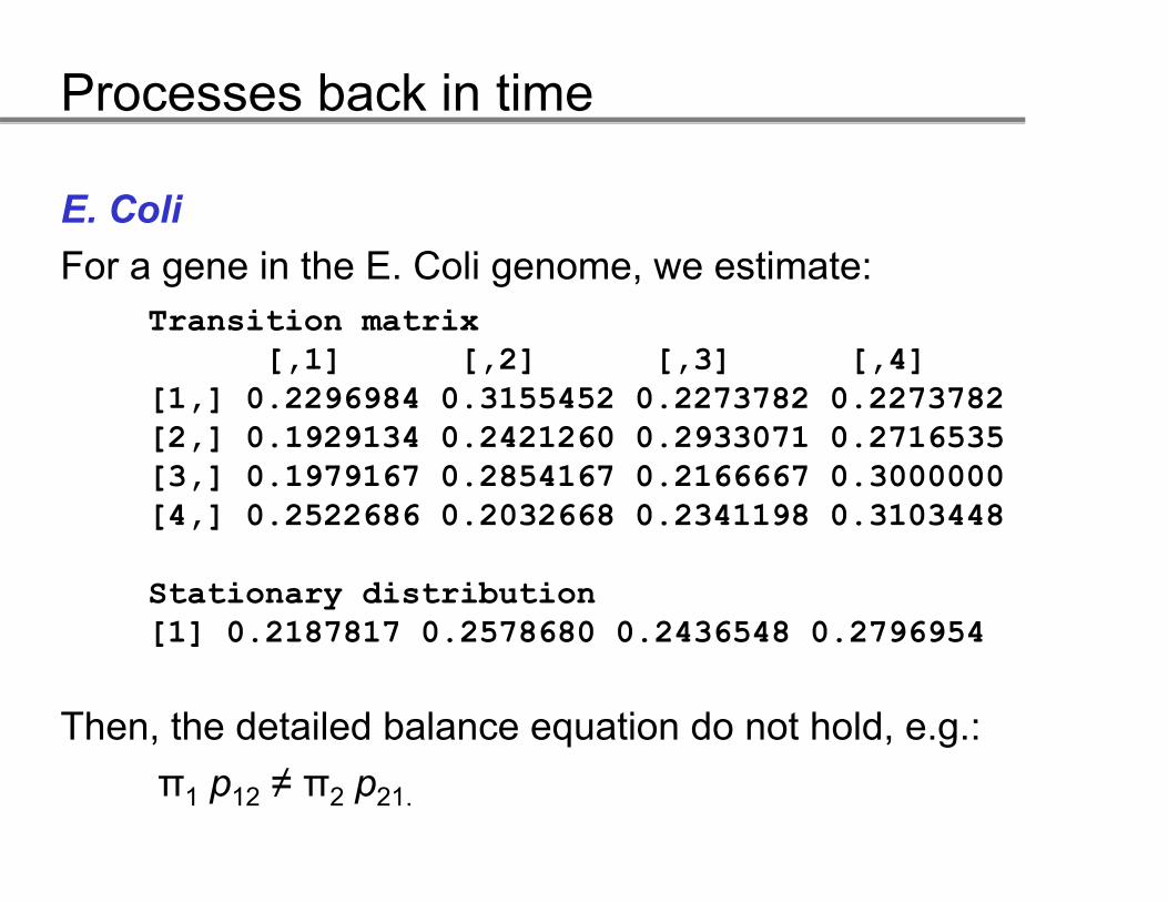
E. ColiFor a gene in the E. Coli genome, we estimate:
Then, the detailed balance equation do not hold, e.g.:π p ≠ π pπ1 p12 ≠ π2 p21.
Processes back in time
NoteWithin evolution theory the notion of irreversibility refers to the presumption that complex organisms once lost evolution will not appear in the same form.
Indeed, the likelihood of reconstructing a particular phylogenic system is infinitesimal small.
Application:Application:motifsmotifs
Application: motifs
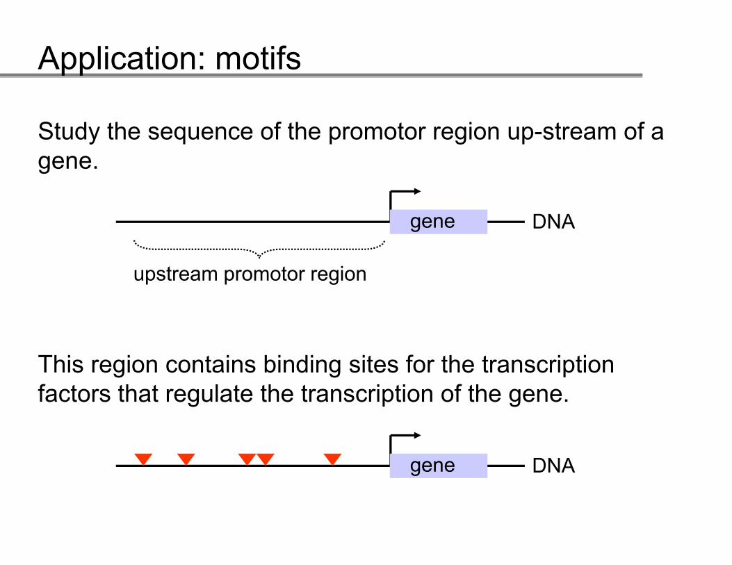
Study the sequence of the promotor region up-stream of a gene.
DNADNAgene
upstream promotor regionp p g
This region contains binding sites for the transcription factors that regulate the transcription of the gene.
DNAgene
Application: motifs
The binding sites of a transciption factor (that may regulate multiple genes) share certain sequence patterns, motifs.
Not all transcription factors and motifs are known. Hence, a p ,high occurrence of a particular sequence pattern in the upstream regions of a gene may indicate that it has a
f ( )regulatory function (e.g., binding site).
ProblemDetermine the probability of observing m motifs in a background generated by a 1st order stationary Markov chainchain.
Application: motifs
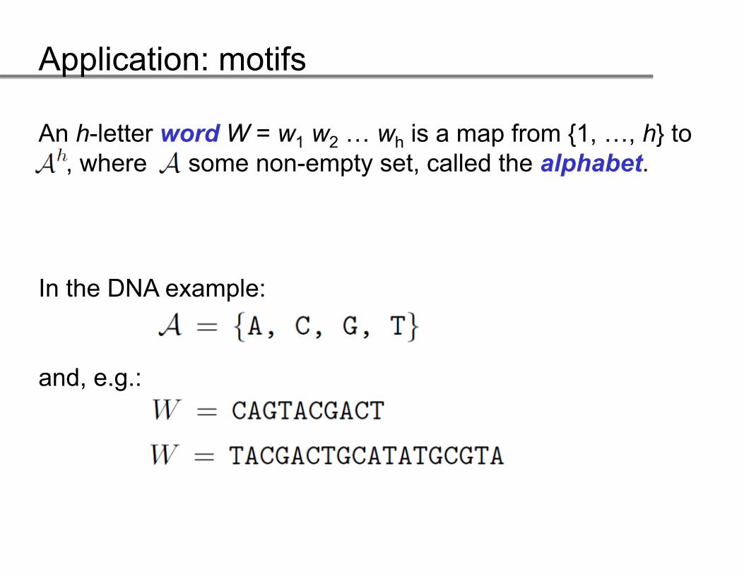
An h-letter word W = w1 w2 … wh is a map from {1, …, h} to, where some non-empty set, called the alphabet.
In the DNA example:In the DNA example:
and, e.g.:
Application: motifs
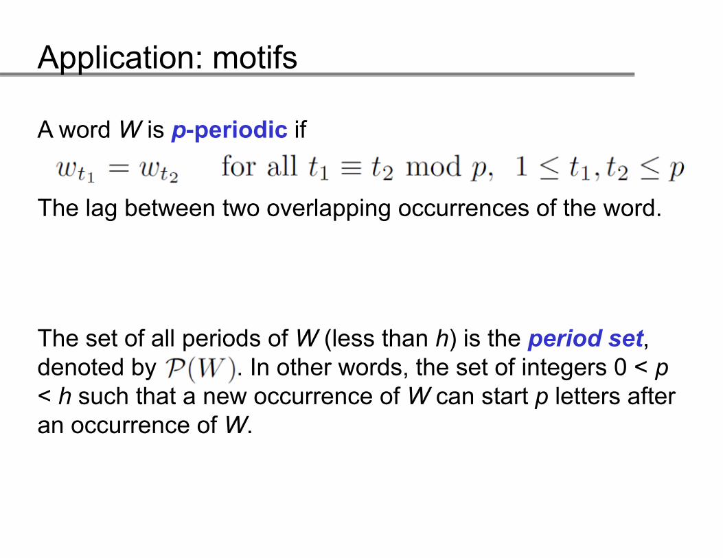
A word W is p-periodic if
The lag between two overlapping occurrences of the wordThe lag between two overlapping occurrences of the word.
The set of all periods of W (less than h) is the period set, p ( ) p ,denoted by . In other words, the set of integers 0 < p< h such that a new occurrence of W can start p letters after an occurrence of W.
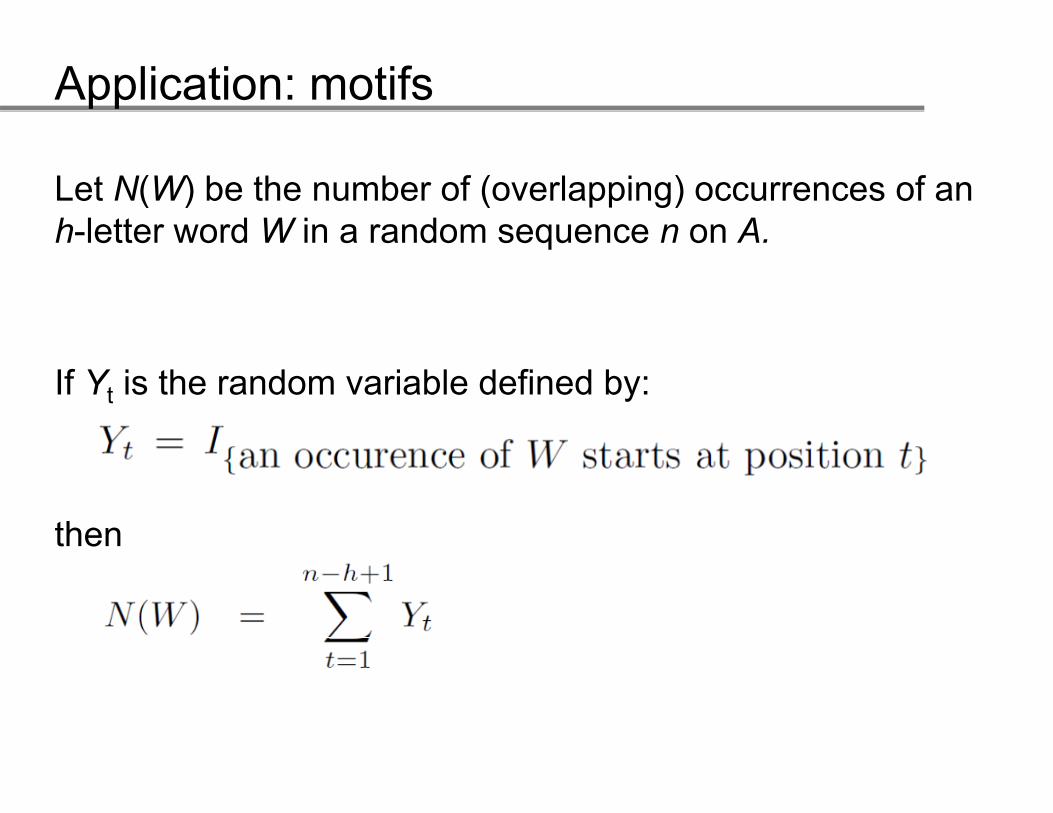
Let N(W) be the number of (overlapping) occurrences of an h-letter word W in a random sequence n on A.
If Yt is the random variable defined by:
then
Application: motifs
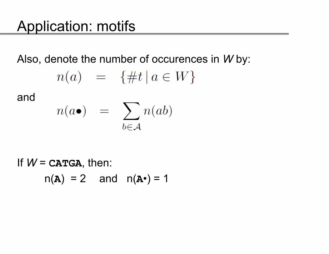
Also, denote the number of occurences in W by:
andand
If W = CATGA, then:n(A) = 2 and n(A•) = 1
Application: motifs
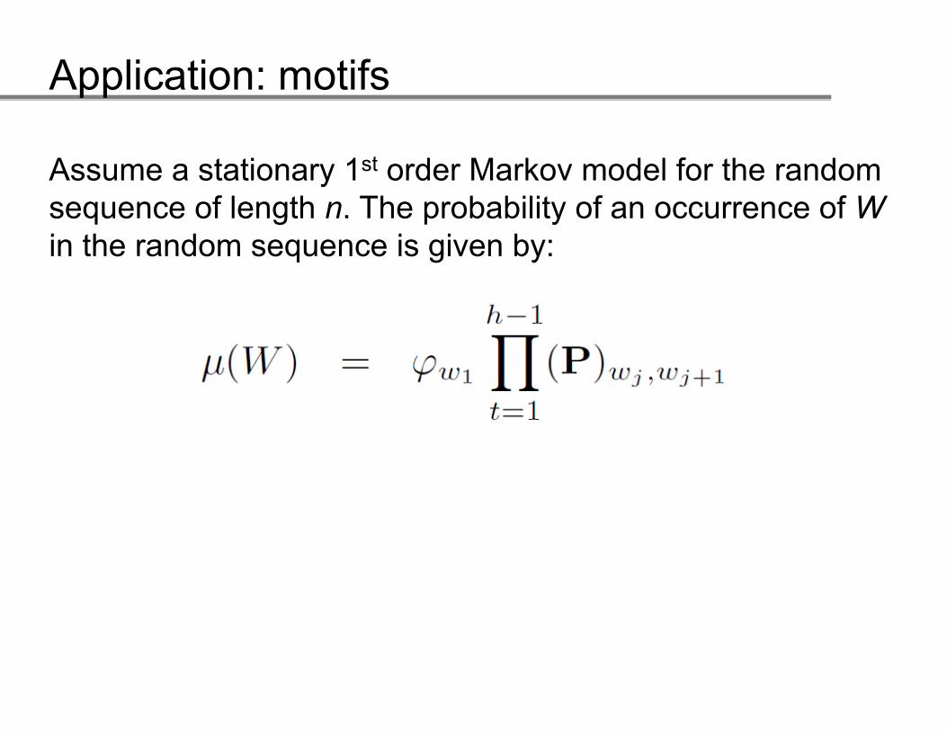
Assume a stationary 1st order Markov model for the random sequence of length n. The probability of an occurrence of Win the random sequence is given by:
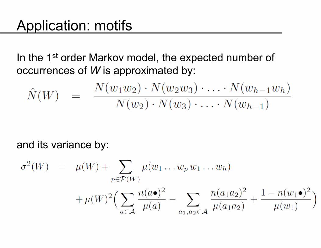
Application: motifs
In the 1st order Markov model, the expected number of occurrences of W is approximated by:
and its variance by:
Application: motifs
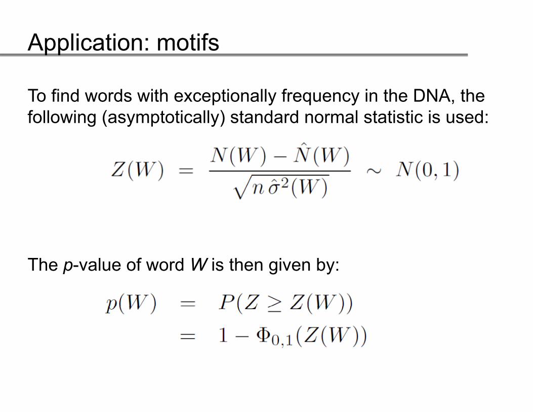
To find words with exceptionally frequency in the DNA, the following (asymptotically) standard normal statistic is used:
The p-value of word W is then given by:
Application: motifs
NoteRobin, Daudon (1999) provide exact probabilities of word occurences in random sequences.
However, Robin, Schbath (2001) point out that calculation of the exact probabilities is computationally intensive. Hence, the use of an approximation here.
References &References & further readingfurther reading
References and further readingEwens, W.J, Grant, G (2006), Statistical Methods for Bioinformatics,
Springer New YorkSpringer, New York.Reinert, G., Schbath, S., Waterman, M.S. (2000), “Probabilistic and
statistical properties of words: an overview”, Journal of C t ti l Bi l 7 1 46Computational Biology, 7, 1-46.
Robin, S., Daudin, J.-J. (1999), “Exact distribution of word occurrences in a random sequence of letters”, Journal of Appliedoccurrences in a random sequence of letters , Journal of Applied Probability, 36, 179-193.
Robin, S., Schbath, S. (2001), “Numerical comparison of several i ti f th d t di t ib ti i dapproximations of the word count distribution in random
sequences”, Journal of Computational Biology, 8(4), 349-359. Schbath, S. (2000), “An overview on the distribution of word countsSchbath, S. (2000), An overview on the distribution of word counts
in Markov chains”, Journal of Computational. Biology, 7, 193-202.Schbath, S., Robin, R. (2009), “How can pattern statistics be useful
f DNA tif di ?” I S St ti ti M th d dfor DNA motif discovery?”. In Scan Statistics: Methods and Applications by Glaz, J. et al. (eds.).
This material is provided under the Creative CommonsThis material is provided under the Creative Commons Attribution/Share-Alike/Non-Commercial License.