77
Copyright © 2013 Pearson Education, Inc. Publishing as Prentice Hall. Cost Behavior Chapter 6 1
| Date post: | 17-Dec-2015 |
| Category: |
Documents |
| Upload: | norman-barnett |
| View: | 219 times |
| Download: | 5 times |

Copyright © 2013 Pearson Education, Inc. Publishing as Prentice Hall.
Cost Behavior
Chapter 6
1

Copyright © 2013 Pearson Education, Inc. Publishing as Prentice Hall.
Objective 1Describe key characteristics and graphs
of various cost behaviors
2

Copyright © 2013 Pearson Education, Inc. Publishing as Prentice Hall. 3
Cost Behavior
Cost behavior—how costs change as volume changes.
There are three common cost behaviors: 1. Variable costs2. Fixed costs3. Mixed costs
Copyright © 2013 Pearson Education, Inc. Publishing as Prentice Hall. 4
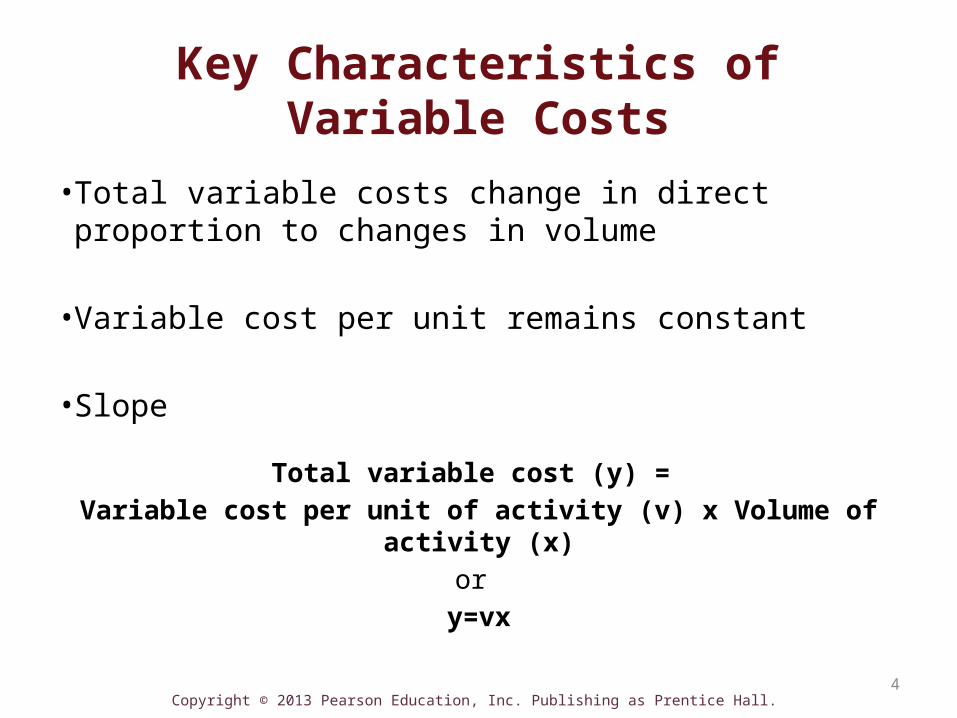
Key Characteristics of Variable Costs
• Total variable costs change in direct proportion to changes in volume
• Variable cost per unit remains constant
• Slope
Total variable cost (y) = Variable cost per unit of activity (v) x Volume of activity (x)
or y=vx

Copyright © 2013 Pearson Education, Inc. Publishing as Prentice Hall. 5
Cost Graphs
• Vertical (y-axis) always shows total costs• Horizontal axis (x-axis) shows volume of
activity
TotalCosts
Total volume of activity
Note that the variable cost per customer remains constant in each of the graphs.

Copyright © 2013 Pearson Education, Inc. Publishing as Prentice Hall. 6
Total Variable Costs

Copyright © 2013 Pearson Education, Inc. Publishing as Prentice Hall.
Objective 2Use cost equations to express and
predict costs
7
Copyright © 2013 Pearson Education, Inc. Publishing as Prentice Hall. 8
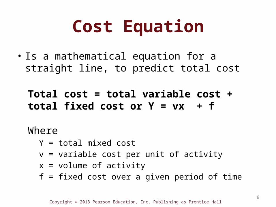
Cost Equation
• Is a mathematical equation for a straight line, to predict total cost
Total cost = total variable cost + total fixed cost or Y = vx + f
WhereY = total mixed costv = variable cost per unit of activityx = volume of activityf = fixed cost over a given period of time
Copyright © 2013 Pearson Education, Inc. Publishing as Prentice Hall. 9
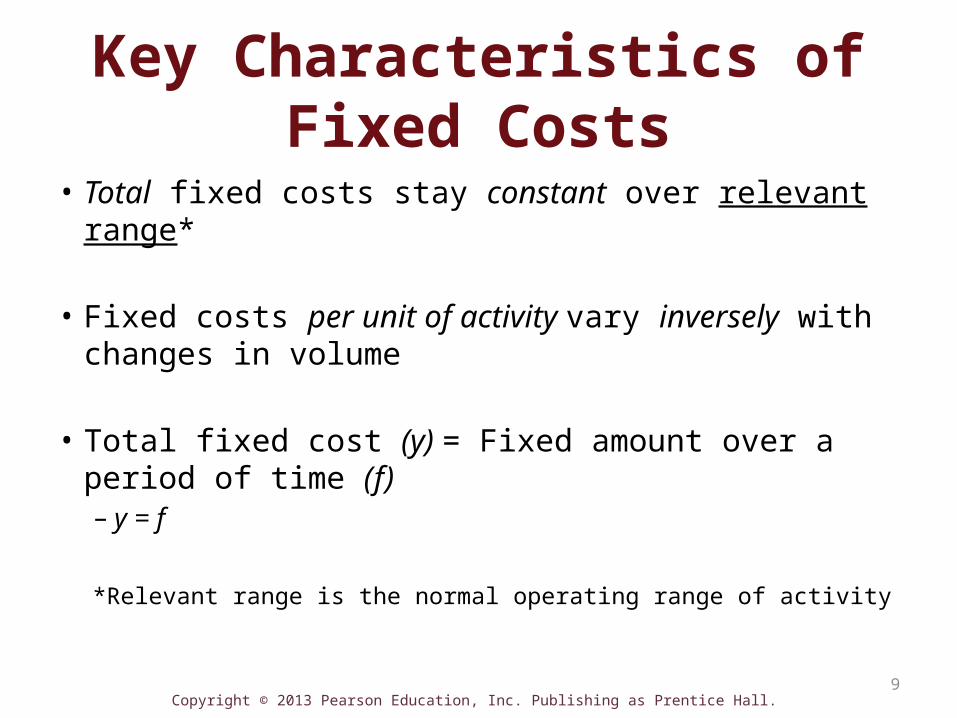
Key Characteristics of Fixed Costs
• Total fixed costs stay constant over relevant range*
• Fixed costs per unit of activity vary inversely with changes in volume
• Total fixed cost (y) = Fixed amount over a period of time (f)– y = f
*Relevant range is the normal operating range of activity

Copyright © 2013 Pearson Education, Inc. Publishing as Prentice Hall. 10
Total Fixed Costs

Copyright © 2013 Pearson Education, Inc. Publishing as Prentice Hall. 11
Costs and Decisions
• Committed fixed costs
• Discretionary fixed costs
Copyright © 2013 Pearson Education, Inc. Publishing as Prentice Hall. 12
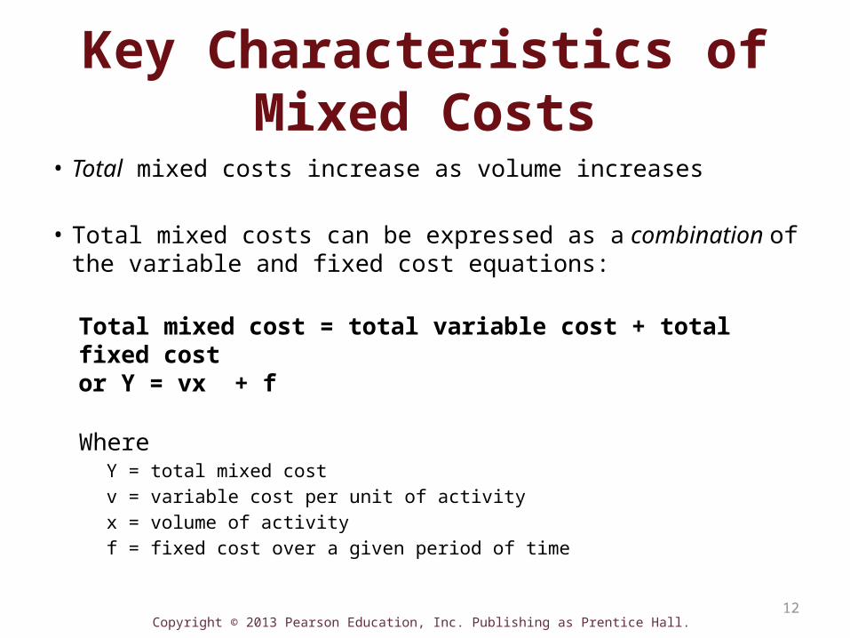
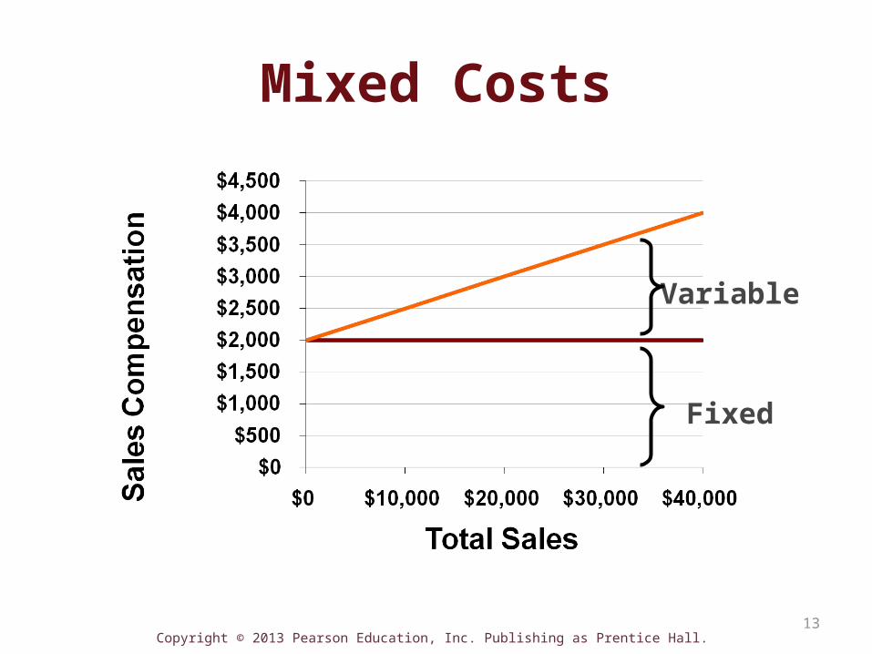
Key Characteristics of Mixed Costs• Total mixed costs increase as volume increases
• Total mixed costs can be expressed as a combination of the variable and fixed cost equations:
Total mixed cost = total variable cost + total fixed cost or Y = vx + f
WhereY = total mixed costv = variable cost per unit of activityx = volume of activityf = fixed cost over a given period of time
Copyright © 2013 Pearson Education, Inc. Publishing as Prentice Hall. 13
Mixed Costs
Variable
Fixed

Copyright © 2013 Pearson Education, Inc. Publishing as Prentice Hall. 14
Now turn to S6-1

Copyright © 2013 Pearson Education, Inc. Publishing as Prentice Hall. 15
S6-1 Identify Cost Behavior
Cost ACost BCost C
Variable CostFixed CostMixed Cost

Copyright © 2013 Pearson Education, Inc. Publishing as Prentice Hall. 16
Relevant Range
• Band of volume where total fixed costs remain constant at a certain level
• Variable costs per unit remain constant at a certain level

Copyright © 2013 Pearson Education, Inc. Publishing as Prentice Hall. 17
Other Cost Behaviors
Step Costs
Copyright © 2013 Pearson Education, Inc. Publishing as Prentice Hall. 18
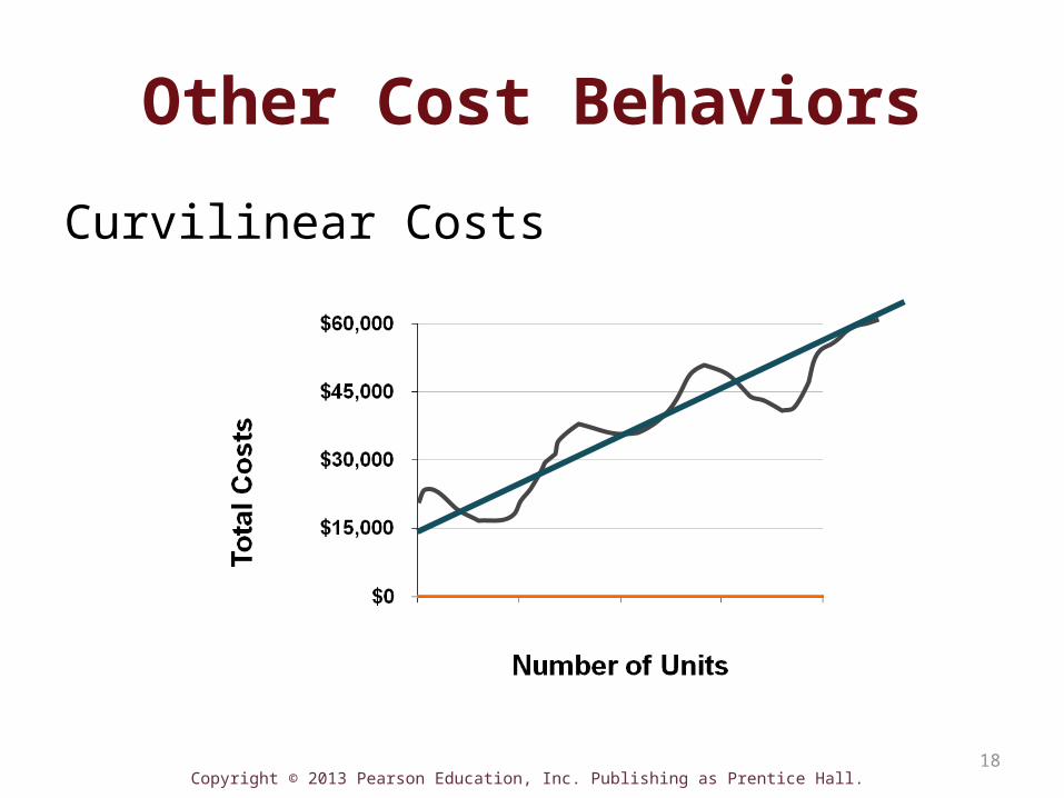
Other Cost Behaviors
Curvilinear Costs
Copyright © 2013 Pearson Education, Inc. Publishing as Prentice Hall. 19
Now turn to E6-22A
Copyright © 2013 Pearson Education, Inc. Publishing as Prentice Hall. 20
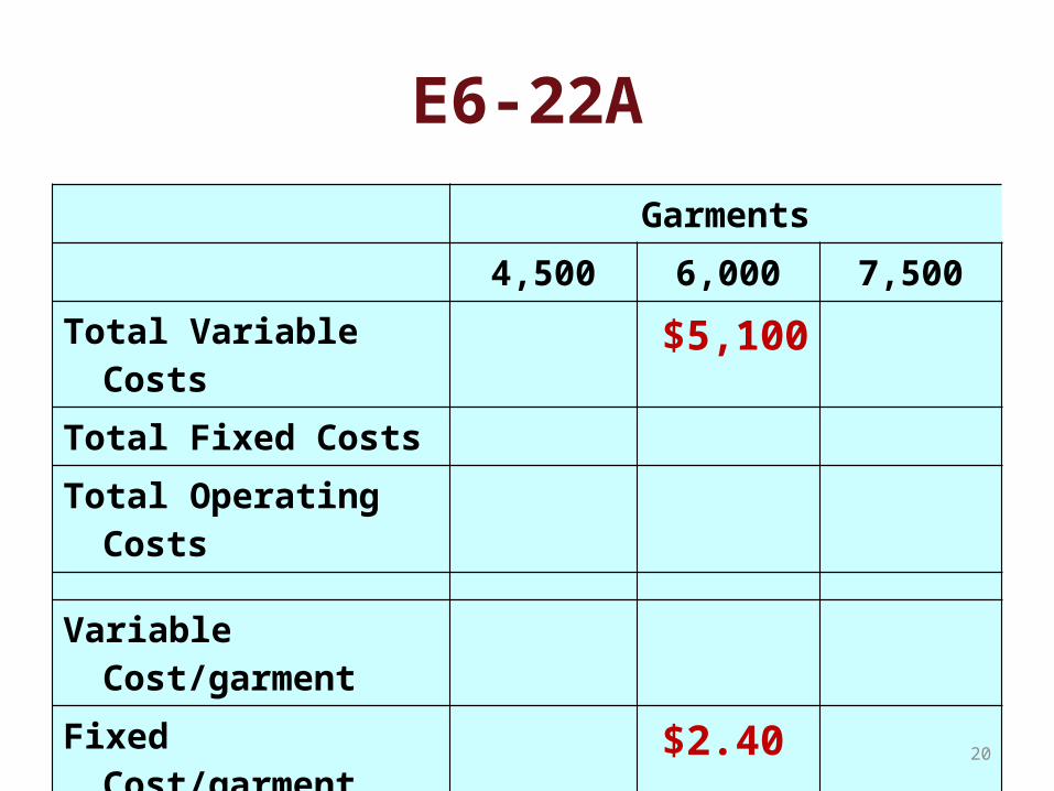
E6-22AGarments
4,500 6,000 7,500Total Variable Costs $5,100Total Fixed CostsTotal Operating Costs
Variable Cost/garment
Fixed Cost/garment $2.40
Average cost/garment
Copyright © 2013 Pearson Education, Inc. Publishing as Prentice Hall. 21
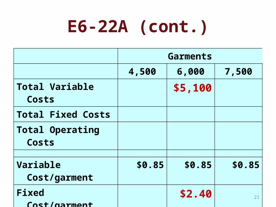
E6-22A (cont.)Garments
4,500 6,000 7,500Total Variable Costs $5,100Total Fixed CostsTotal Operating Costs
Variable Cost/garment $0.85 $0.85 $0.85
Fixed Cost/garment $2.40
Average cost/garment
Copyright © 2013 Pearson Education, Inc. Publishing as Prentice Hall. 22
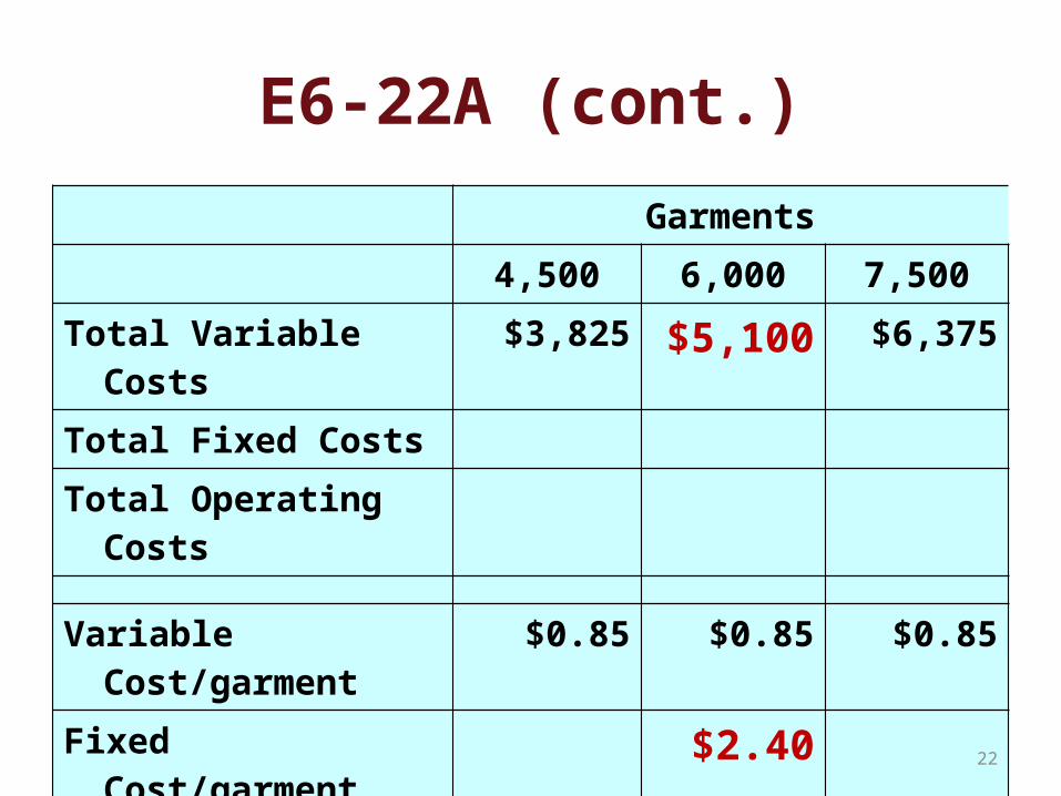
E6-22A (cont.)Garments
4,500 6,000 7,500Total Variable Costs $3,825 $5,100 $6,375Total Fixed CostsTotal Operating Costs
Variable Cost/garment $0.85 $0.85 $0.85
Fixed Cost/garment $2.40
Average cost/garment

Copyright © 2013 Pearson Education, Inc. Publishing as Prentice Hall. 23
E6-22A (cont.)Garments
4,500 6,000 7,500Total Variable Costs $3,825 $5,100 $6,375Total Fixed Costs $14,400 $14,400 $14,400Total Operating Costs
Variable Cost/garment $0.85 $0.85 $0.85
Fixed Cost/garment $2.40
Average cost/garment

Copyright © 2013 Pearson Education, Inc. Publishing as Prentice Hall. 24
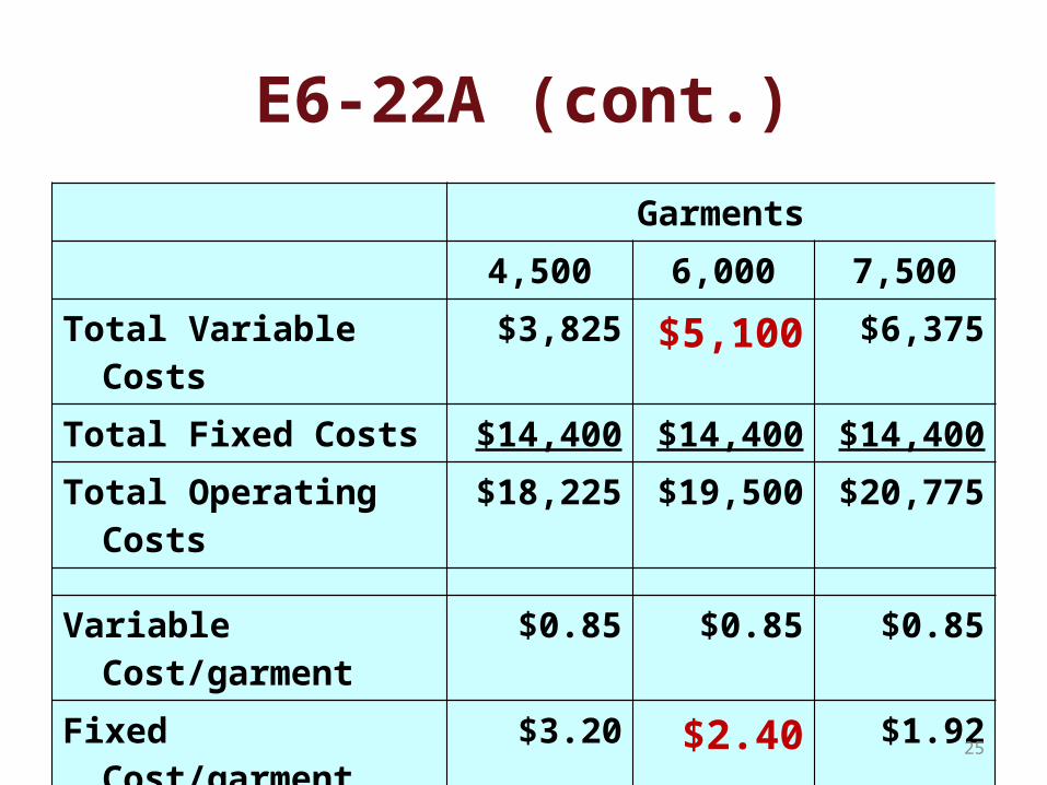
E6-22A (cont.)Garments
4,500 6,000 7,500Total Variable Costs $3,825 $5,100 $6,375Total Fixed Costs $14,400 $14,400 $14,400Total Operating Costs $18,225 $19,500 $20,775
Variable Cost/garment $0.85 $0.85 $0.85
Fixed Cost/garment $2.40
Average cost/garment
Copyright © 2013 Pearson Education, Inc. Publishing as Prentice Hall. 25
E6-22A (cont.)Garments
4,500 6,000 7,500Total Variable Costs $3,825 $5,100 $6,375Total Fixed Costs $14,400 $14,400 $14,400Total Operating Costs $18,225 $19,500 $20,775
Variable Cost/garment $0.85 $0.85 $0.85
Fixed Cost/garment $3.20 $2.40 $1.92
Average cost/garment

Copyright © 2013 Pearson Education, Inc. Publishing as Prentice Hall. 26
E6-22A (cont.)Garments
4,500 6,000 7,500Total Variable Costs $3,825 $5,100 $6,375Total Fixed Costs $14,400 $14,400 $14,400Total Operating Costs $18,225 $19,500 $20,775
Variable Cost/garment $0.85 $0.85 $0.85
Fixed Cost/garment $3.20 $2.40 $1.92
Average cost/garment $4.05 $3.25 $2.77

Copyright © 2013 Pearson Education, Inc. Publishing as Prentice Hall. 27
E6-22A (cont.)
The average cost per garment changes as volume changes, due to the fixed component of the dry cleaner’s costs. The fixed cost per unit decrease as volume increases, while the variable cost per unit remains constant.
Actual costs at 4,500 garments$12,465 Total predicted costs ($2.77 × 4,500 garments)(18,225) Actual costs at 4,500 garments$5,760 Difference (underestimated)

Copyright © 2013 Pearson Education, Inc. Publishing as Prentice Hall. 28
Now turn to E6-25A

Copyright © 2013 Pearson Education, Inc. Publishing as Prentice Hall. 29
E6-25A
Data: Freedom Mailbox produces decorative mailboxes. The company’s average cost per unit is $24.43 when it produces 1,300 mailboxes.
1. 1,300 x $24.43 $31,759
2. Total costs $31,759Less total fixed costs (21,359)Total variable costs $10,400
÷ 1,300 Variable cost per mailbox $8.00
Copyright © 2013 Pearson Education, Inc. Publishing as Prentice Hall. 30
E6-25A
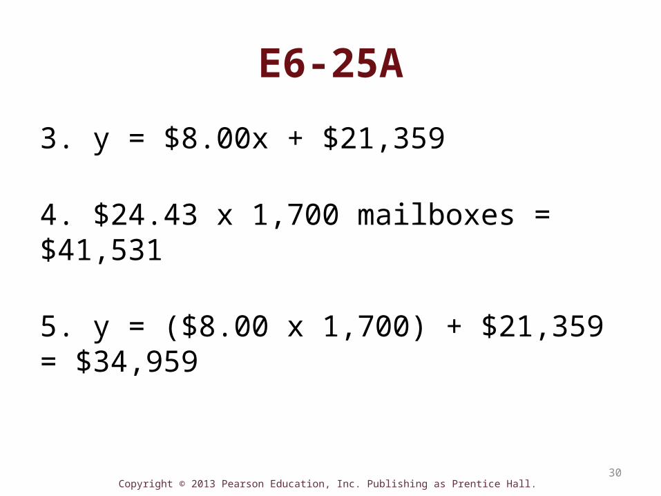
3. y = $8.00x + $21,359
4. $24.43 x 1,700 mailboxes = $41,531
5. y = ($8.00 x 1,700) + $21,359 = $34,959

Copyright © 2013 Pearson Education, Inc. Publishing as Prentice Hall. 31
E6-25A
6. Using average at 1,700 $41,531 Using cost equation $34,959
$6,572

Copyright © 2013 Pearson Education, Inc. Publishing as Prentice Hall. 32
Sustainability and Cost Behavior
• Sustainable companies and changes in cost behavior• E-banking and e-billing drive down variable
costs• Greener lifestlyes• Environmental Impact
Copyright © 2013 Pearson Education, Inc. Publishing as Prentice Hall.
Objective 3Use account analysis and scatter plots to
analyze cost behavior
33

Copyright © 2013 Pearson Education, Inc. Publishing as Prentice Hall. 34
Cost Behavior Analysis
• Four methods to analyze cost behavior– Account Analysis– Scatter Plots– High-Low Method– Regression Analysis

Copyright © 2013 Pearson Education, Inc. Publishing as Prentice Hall. 35
Account Analysis
• Use of judgment to classify each general ledger account as variable, fixed, or mixed
• Subjective

Copyright © 2013 Pearson Education, Inc. Publishing as Prentice Hall. 36
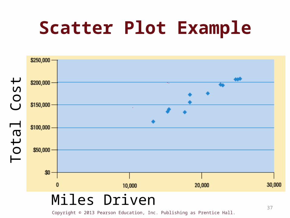
Scatter Plots
• Use historical data to determine a cost’s behavior
• Scatter plot is the graph of historical cost data on the y-axis and volume data on the x-axis
• Helps managers visually determine how strong the relationship is between the cost and the volume of the chosen activity base
Copyright © 2013 Pearson Education, Inc. Publishing as Prentice Hall. 37
Scatter Plot Example
Miles Driven
Tota
l Cos
t

Copyright © 2013 Pearson Education, Inc. Publishing as Prentice Hall.
Objective 4Use the high-low method to analyze
cost behavior
38

Copyright © 2013 Pearson Education, Inc. Publishing as Prentice Hall. 39
High-Low Method
Step 1: Find variable cost per unit (slope) of cost line Step 2: Find the fixed costs (vertical intercept)Step 3: Create the cost equation
Advantage: Easy to useDisadvantage: Only uses 2 data points

Copyright © 2013 Pearson Education, Inc. Publishing as Prentice Hall. 40
Turn to E6-28A

Copyright © 2013 Pearson Education, Inc. Publishing as Prentice Hall. 41
High-Low Method: E6-28A
• Step 1: Find slope of the mixed cost line
(variable cost/unit) = Δ in cost (y) / Δ in volume (x)
• The slope represents the variable cost per unit of activity
($5,730 -$5,040) ÷ (18,500-15,500)$690 ÷ 3,000 = $0.23

Copyright © 2013 Pearson Education, Inc. Publishing as Prentice Hall. 42
High-Low Method: E6-28A (cont.)
• Step 2: Find the vertical intercept
Fixed costs = Total mixed cost – Total variable cost
$5,730 – ($0.23 • 18,500) = $1,475OR$5,040 – ($0.23 • 15,500) = $1,475
Copyright © 2013 Pearson Education, Inc. Publishing as Prentice Hall. 43
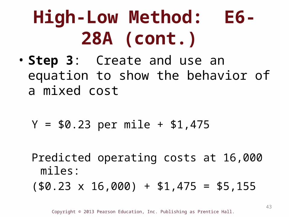
High-Low Method: E6-28A (cont.)
• Step 3: Create and use an equation to show the behavior of a mixed cost
Y = $0.23 per mile + $1,475
Predicted operating costs at 16,000 miles:($0.23 x 16,000) + $1,475 = $5,155

Copyright © 2013 Pearson Education, Inc. Publishing as Prentice Hall.
Objective 5Use regression analysis to analyze
cost behavior
44

Copyright © 2013 Pearson Education, Inc. Publishing as Prentice Hall. 45
Regression Analysis – Exhibit 6-15
• Statistical procedure to find the line that best fits data (cost equation)
• Uses all data points• R-square, Intercept, X Variable 1
Copyright © 2013 Pearson Education, Inc. Publishing as Prentice Hall. 46
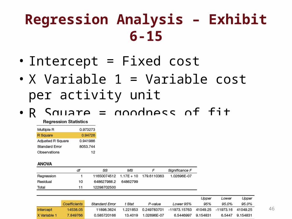
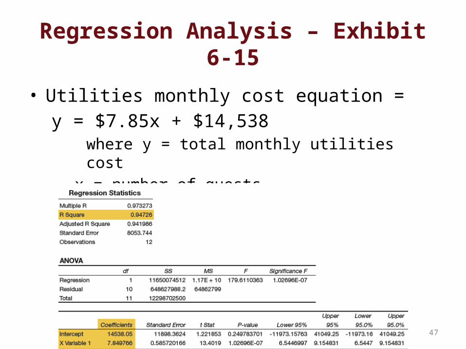
Regression Analysis – Exhibit 6-15
• Intercept = Fixed cost• X Variable 1 = Variable cost per activity unit• R Square = goodness of fit
Copyright © 2013 Pearson Education, Inc. Publishing as Prentice Hall. 47
Regression Analysis – Exhibit 6-15
• Utilities monthly cost equation =y = $7.85x + $14,538
where y = total monthly utilities costx = number of guests

Copyright © 2013 Pearson Education, Inc. Publishing as Prentice Hall. 48
R-Square Value
• “Goodness of fit”
• How well does the line fit the data points?
• Ranges from 0 to 1
Copyright © 2013 Pearson Education, Inc. Publishing as Prentice Hall. 49
Predicting Costs & Data Concerns
• Data Concerns– Only valid within relevant range– Seasonal variations– Inflation– Outliers – abnormal data points

Copyright © 2013 Pearson Education, Inc. Publishing as Prentice Hall.
Objective 6Describe variable costing and prepare a contribution margin income statement
50

Copyright © 2013 Pearson Education, Inc. Publishing as Prentice Hall. 51
Absorption Costing
• Required by GAAP for external reporting
• Assign all manufacturing costs to products (DM, DL, Variable MOH, and Fixed MOH)
• Traditional (conventional) income statement

Copyright © 2013 Pearson Education, Inc. Publishing as Prentice Hall. 52
Traditional (Conventional) Income Statement
Sales- Cost of Goods Sold Gross Margin- Selling, general, and administrative costs Operating Income

Copyright © 2013 Pearson Education, Inc. Publishing as Prentice Hall. 53
Variable Costing• Assigns only variable manufacturing costs to
products (DM, DL, and Variable MOH)
• Fixed manufacturing overhead = period cost
• For internal management decisions
• Contribution Margin income statement
Copyright © 2013 Pearson Education, Inc. Publishing as Prentice Hall. 54
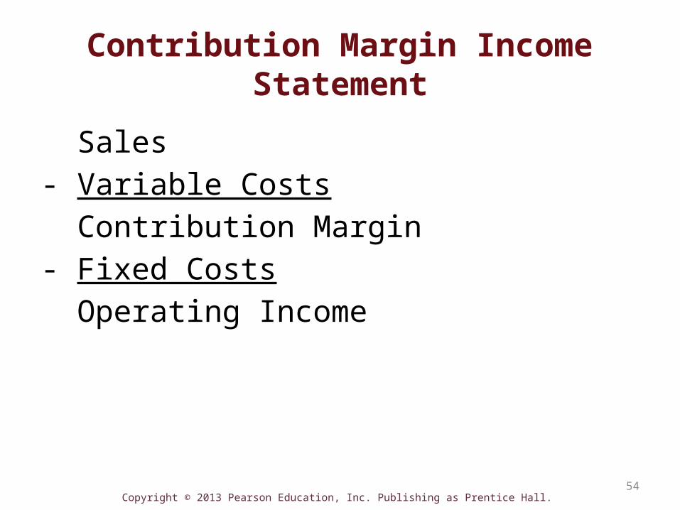
Contribution Margin Income Statement
Sales- Variable Costs Contribution Margin- Fixed Costs Operating Income

Copyright © 2013 Pearson Education, Inc. Publishing as Prentice Hall. 55
Reconciling Operating Income Between the Two Costing Systems
• Difference in Operating Income = (Change in inventory level, in units) x (Fixed MOH per unit)
Copyright © 2013 Pearson Education, Inc. Publishing as Prentice Hall. 56
Now turn to E6-44A
Copyright © 2013 Pearson Education, Inc. Publishing as Prentice Hall.
E6-44AConventional (Absorption Costing) Income Statement

Copyright © 2013 Pearson Education, Inc. Publishing as Prentice Hall.
E6-44AConventional (Absorption Costing) Income Statement
Sales revenue (205,000 $44) $9,020,000

Copyright © 2013 Pearson Education, Inc. Publishing as Prentice Hall.
E6-44AConventional (Absorption Costing) Income Statement
Sales revenue (205,000 $44) $9,020,000
Less: Cost of Goods Sold (205,000 x $26) ( 5,330,000)
• Fixed mfg per unit = $2,475,000 fixed MOH / 225,000 units produced = $11 per unit• Variable MOH per unit $15 (given)• Total manufacturing cost per unit = $11 + $15 = $26

Copyright © 2013 Pearson Education, Inc. Publishing as Prentice Hall.
E6-44AConventional (Absorption Costing) Income Statement
Sales revenue (205,000 $44) $9,020,000
Less: Cost of Goods Sold (205,000 x $26) ( 5,330,000)
Gross Profit 3,690,000
Operating Expenses [(205,000 x $6) + $250,000] (1,480,000)
Operating Income $2,210,000
• Fixed mfg per unit = $2,475,000 fixed MOH / 225,000 units produced = $11 per unit• Variable MOH per unit $15 (given)• Total manufacturing cost per unit = $11 + $15 = $26

Copyright © 2013 Pearson Education, Inc. Publishing as Prentice Hall. 63
E6-44A (cont.)
Now we turn to the Contribution Margin Income Statement (VARIABLE COSTING STMT)
First need to calculate:Variable cost of goods sold

Copyright © 2013 Pearson Education, Inc. Publishing as Prentice Hall. 64
E6-44A (cont.)• Variable cost of goods sold:
Beginning finished goods inventory $ 0Variable cost of goods manufactured ($15
x 225,000) 3,375,000Variable cost of goods available
for sale 3,375,000Ending fin. goods inv. ($15 x 20,000) (300,000)Variable cost of goods sold*
$3,075,000*Also can calculate as 205,000 units x $15 = $3,075,000

Copyright © 2013 Pearson Education, Inc. Publishing as Prentice Hall. 65
E6-44A (cont.)Contribution Margin (Variable Costing) Income Statement
Sales revenue (205,000 $44) $9,020,000

Copyright © 2013 Pearson Education, Inc. Publishing as Prentice Hall. 66
E6-44A (cont.)Contribution Margin (Variable Costing) Income Statement
Sales revenue (205,000 $44) $9,020,000
Variable expenses:
Variable COGS (from prior calculation)
$3,075,000*

Copyright © 2013 Pearson Education, Inc. Publishing as Prentice Hall. 67
E6-44A (cont.)Contribution Margin (Variable Costing) Income Statement
Sales revenue (205,000 $44) $9,020,000
Variable expenses:
Variable COGS (from prior calculation)
$3,075,000*
Sales comm expense ($6x205,000) 1,230,000 (4,305,000)

Copyright © 2013 Pearson Education, Inc. Publishing as Prentice Hall. 68
E6-44A (cont.)Contribution Margin (Variable Costing) Income Statement
Sales revenue (205,000 $44) $9,020,000
Variable expenses:
Variable COGS (from prior calculation)
$3,075,000*
Sales comm expense ($6x205,000) 1,230,000 (4,305,000)
Contribution margin $4,715,000

Copyright © 2013 Pearson Education, Inc. Publishing as Prentice Hall. 69
E6-44A (cont.)Contribution Margin (Variable Costing) Income Statement
Sales revenue (205,000 $44) $9,020,000
Variable expenses:
Variable COGS (from prior calculation)
$3,075,000*
Sales comm expense ($6x205,000) 1,230,000 (4,305,000)
Contribution margin $4,715,000
Fixed expenses:
MOH (given in exercise) $2,475,000
Operating expenses (given) 250,000 (2,725,000)

Copyright © 2013 Pearson Education, Inc. Publishing as Prentice Hall. 70
E6-44A (cont.)Contribution Margin (Variable Costing) Income Statement
Sales revenue (205,000 $44) $9,020,000
Variable expenses:
Variable COGS (from prior calculation)
$3,075,000*
Sales comm expense ($6x205,000) 1,230,000 (4,305,000)
Contribution margin $4,715,000
Fixed expenses:
MOH $2,475,000
Operating expenses 250,000 (2,725,000)
Operating income $1,990,000

Copyright © 2013 Pearson Education, Inc. Publishing as Prentice Hall. 71
E6-44A (cont.)Req. 2 Difference between the two methods:Change in inventory x Fixed MOH per unit = (20,000 x $11*) = $220,000
*$11 is the fixed MOH per unit ($2,475,000 / 225,000)
Traditional method produces the higher operating income because of the fixed MOH still remaining in inventory.
Proof:Traditional operating income $2,210,000Contribution margin operating income 1,990,000Difference $ 220,000

Copyright © 2013 Pearson Education, Inc. Publishing as Prentice Hall. 72
E6-44A (cont.)
Req. 3Incremental analysis:
Increase in contribution margin $460,000 [($44-$21)*20,000 goggles]Increase in fixed costs (145,000)Increase in operating income $315,000
Copyright © 2013 Pearson Education, Inc. Publishing as Prentice Hall. 73
Now turn to S6-16
Copyright © 2013 Pearson Education, Inc. Publishing as Prentice Hall. 74
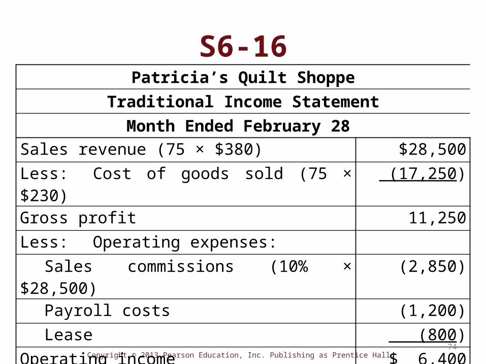
Patricia’s Quilt ShoppeTraditional Income Statement
Month Ended February 28 Sales revenue (75 × $380) $28,500Less: Cost of goods sold (75 × $230) (17,250)Gross profit 11,250Less: Operating expenses:
Sales commissions (10% × $28,500) (2,850)Payroll costs (1,200)Lease (800)
Operating income $ 6,400
S6-16
Copyright © 2013 Pearson Education, Inc. Publishing as Prentice Hall. 75
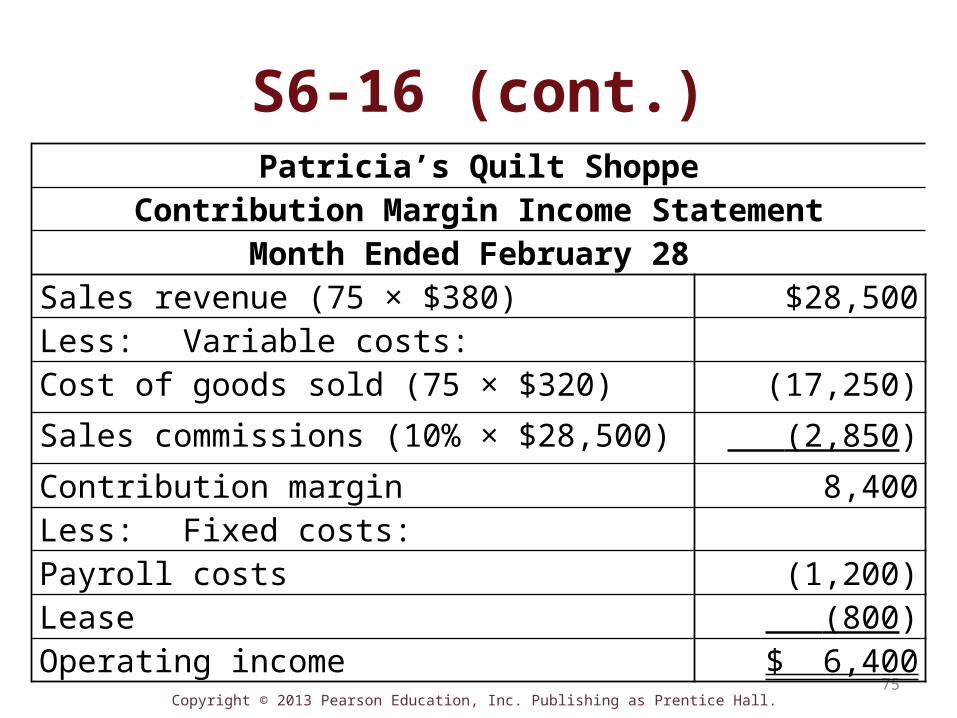
S6-16 (cont.)Patricia’s Quilt Shoppe
Contribution Margin Income StatementMonth Ended February 28
Sales revenue (75 × $380) $28,500Less: Variable costs:Cost of goods sold (75 × $320) (17,250)
Sales commissions (10% × $28,500) (2,850)
Contribution margin 8,400Less: Fixed costs:Payroll costs (1,200)Lease (800)Operating income $ 6,400
Copyright © 2013 Pearson Education, Inc. Publishing as Prentice Hall. 76
Absorption Costing and Manager Incentives
• When inventories increase, absorption costing income is higher than variable costing income.
• When inventories decrease, absorption costing income is lower than variable costing income.
• Therefore…managers may increase production to build up inventory to maximize income and, therefore, their own bonus.

Copyright © 2013 Pearson Education, Inc. Publishing as Prentice Hall. 77
End of Chapter 6


