53
Demand Information Distortion and Bullwhip Effect Chopra: 3 rd ed.: Chap. 17
| Date post: | 25-Mar-2018 |
| Category: |
Documents |
| Upload: | truongminh |
| View: | 219 times |
| Download: | 1 times |
Demand Information Distortion and
Bullwhip Effect
Chopra: 3rd ed.: Chap. 17
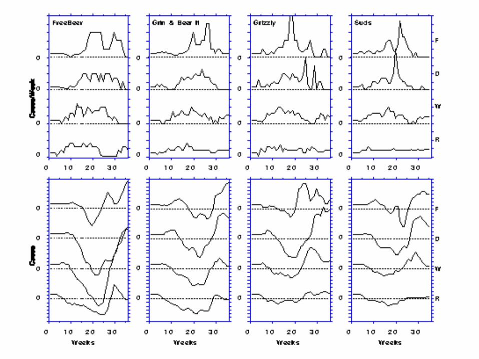
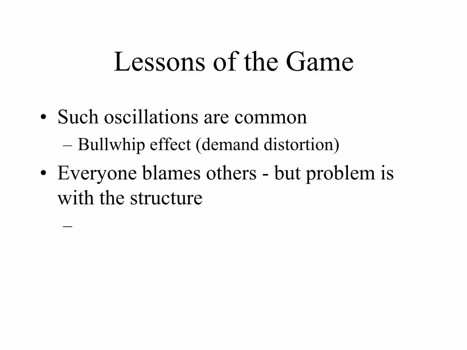
Lessons of the Game
• Such oscillations are common
– Bullwhip effect (demand distortion)
• Everyone blames others - but problem is
with the structure
–
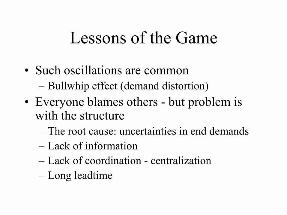
Lessons of the Game
• Such oscillations are common
– Bullwhip effect (demand distortion)
• Everyone blames others - but problem is with the structure
– The root cause: uncertainties in end demands
– Lack of information
– Lack of coordination - centralization
– Long leadtime
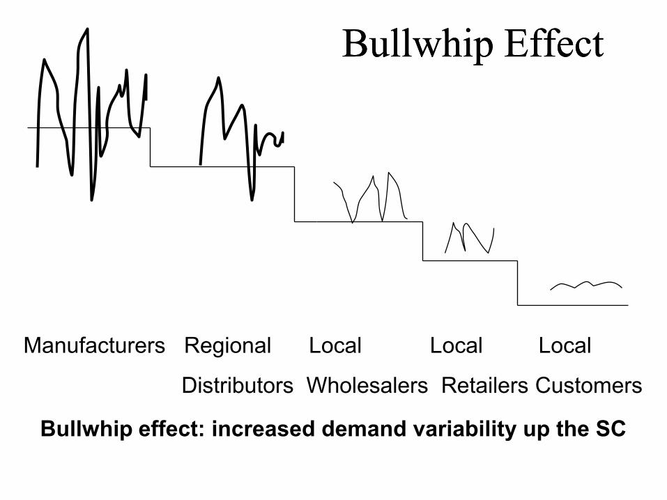
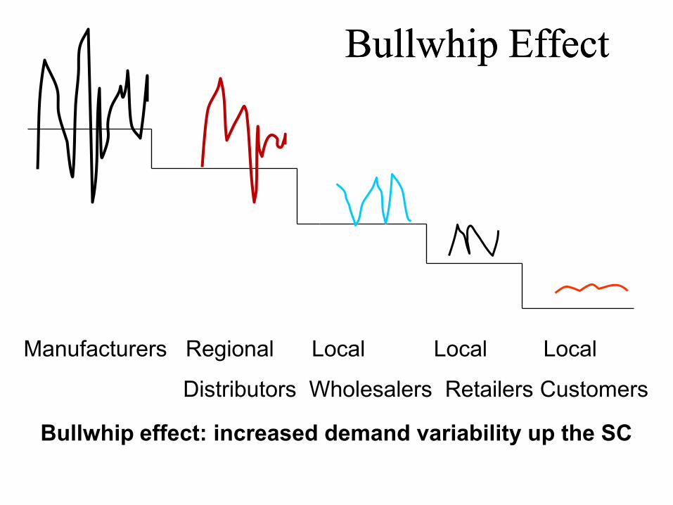
Bullwhip EffectBullwhip Effect
Manufacturers Regional Local Local Local
Distributors Wholesalers Retailers Customers
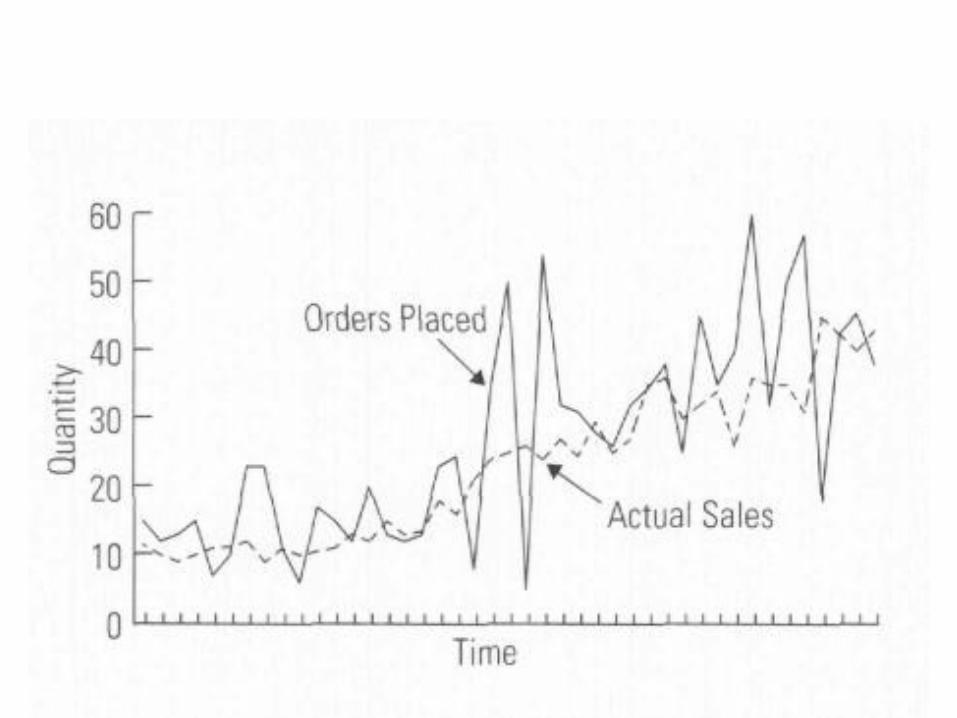
Bullwhip effect: increased demand variability up the SC
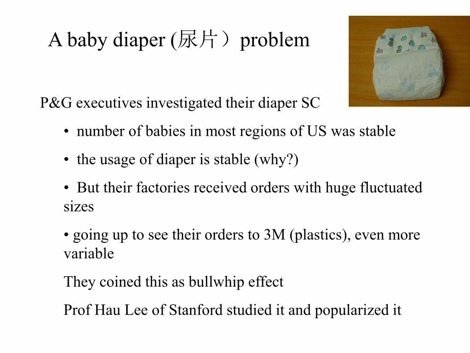
A baby diaper (尿片)problem
P&G executives investigated their diaper SC
• number of babies in most regions of US was stable
• the usage of diaper is stable (why?)
• But their factories received orders with huge fluctuated
sizes
• going up to see their orders to 3M (plastics), even more
variable
They coined this as bullwhip effect
Prof Hau Lee of Stanford studied it and popularized it
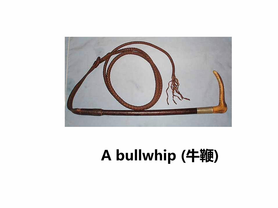
A bullwhip (牛鞭)
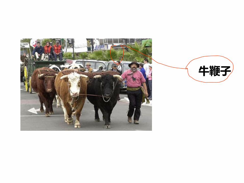
牛鞭子
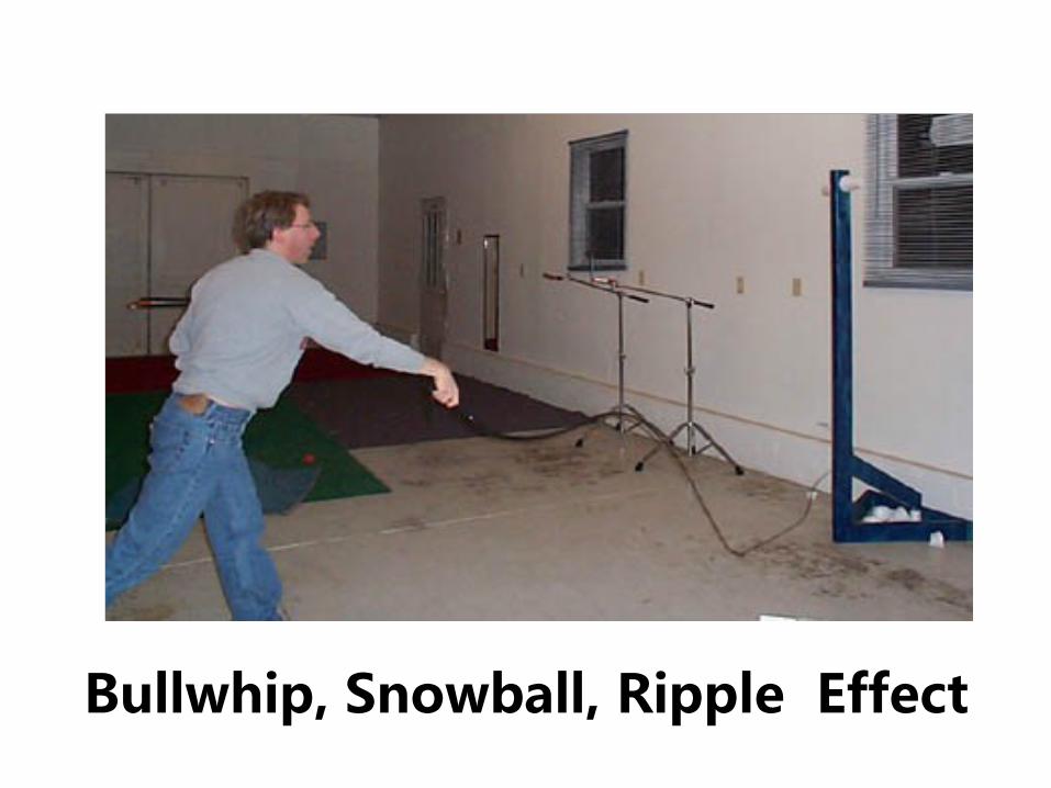
Bullwhip, Snowball, Ripple Effect
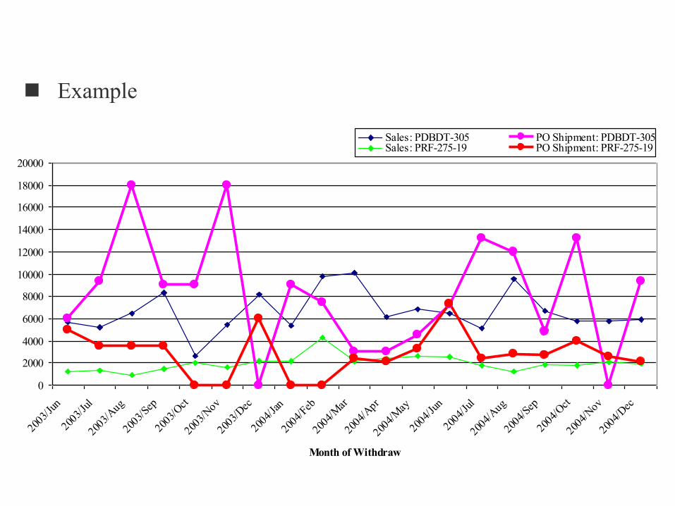
Example
ATO – Sales vs. PO Shipment
0
2000
4000
6000
8000
10000
12000
14000
16000
18000
20000
2003/
Jun
2003/
Jul
2003/
Aug
2003/
Sep
2003/
Oct
2003/
Nov
2003/
Dec
2004/
Jan
2004/
Feb
2004/
Mar
2004/
Apr
2004/
May
2004/
Jun
2004/
Jul
2004/
Aug
2004/
Sep
2004/
Oct
2004/
Nov
2004/
Dec
Month of Withdraw
Sales: PDBDT-305 PO Shipment: PDBDT-305Sales: PRF-275-19 PO Shipment: PRF-275-19

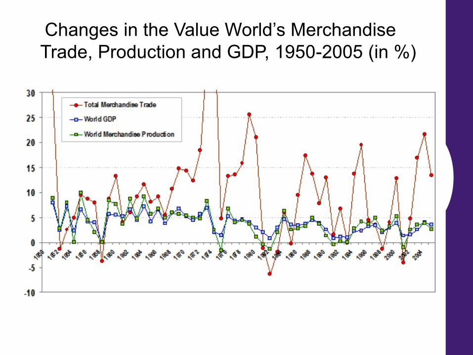
Changes in the Value World’s Merchandise
Trade, Production and GDP, 1950-2005 (in %)
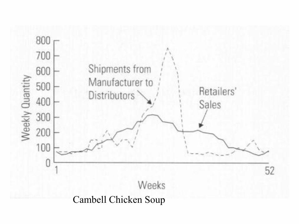
Cambell Chicken Soup
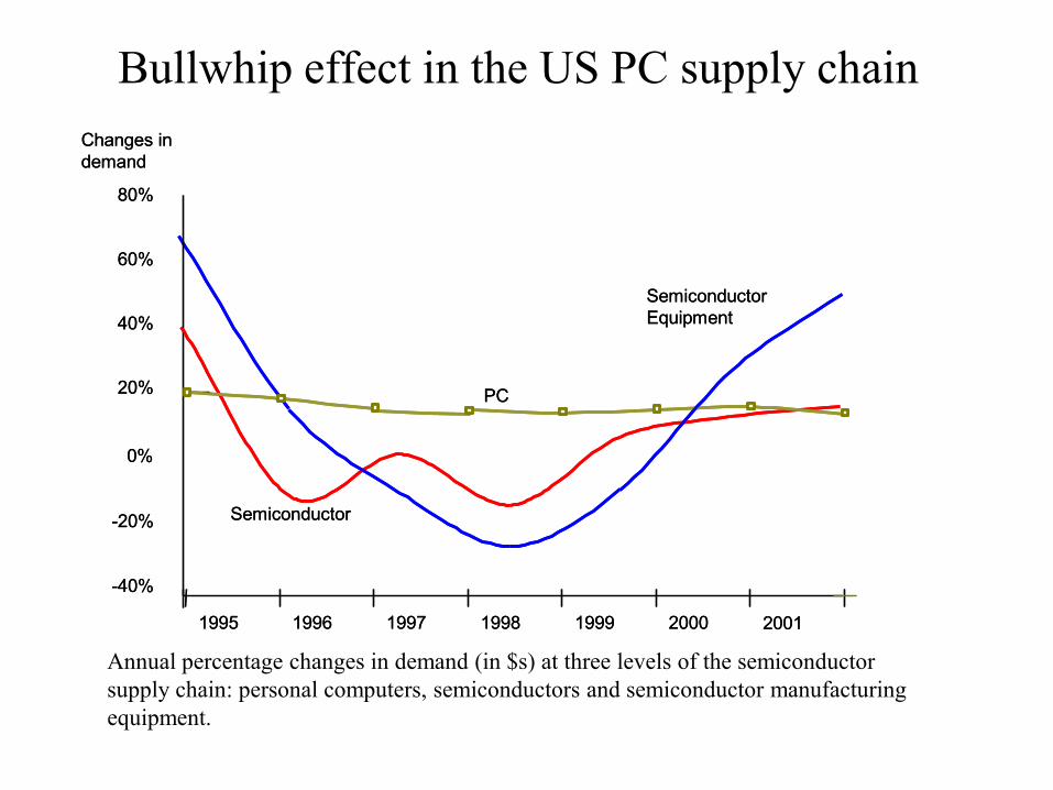
Bullwhip effect in the US PC supply chain
Semiconductor
1995 1996 1997 1998 1999 2000 2001
-40%
-20%
0%
20%
40%
60%
80%
PC
Semiconductor
Equipment
Changes in
demand
Semiconductor
1995 1996 1997 1998 1999 2000 2001
-40%
-20%
0%
20%
40%
60%
80%
PC
Semiconductor
Equipment
Changes in
demand
Annual percentage changes in demand (in $s) at three levels of the semiconductor
supply chain: personal computers, semiconductors and semiconductor manufacturing
equipment.
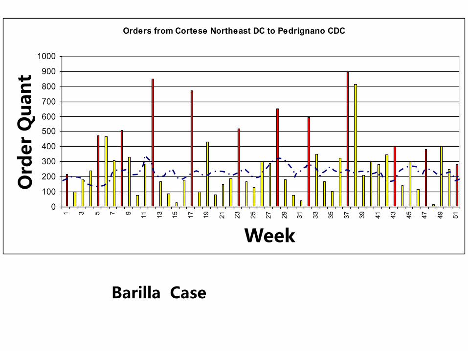
Barilla Case
Orders from Cortese Northeast DC to Pedrignano CDC
0
100
200
300
400
500
600
700
800
900
10001 3 5 7 9
11
13
15
17
19
21
23
25
27
29
31
33
35
37
39
41
43
45
47
49
51
Weeks
Ord
ers
(Q
uin
tals
)
Week
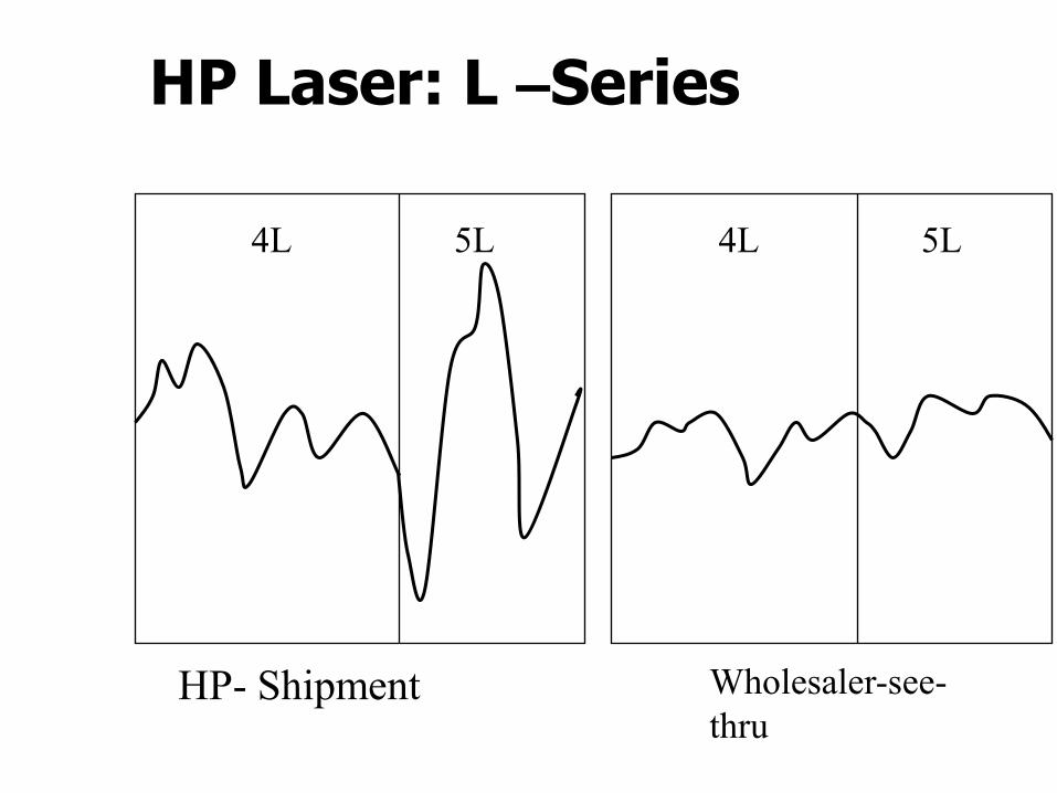
4L 5L 4L 5L
HP- Shipment Wholesaler-see-
thru
HP Laser: L –Series
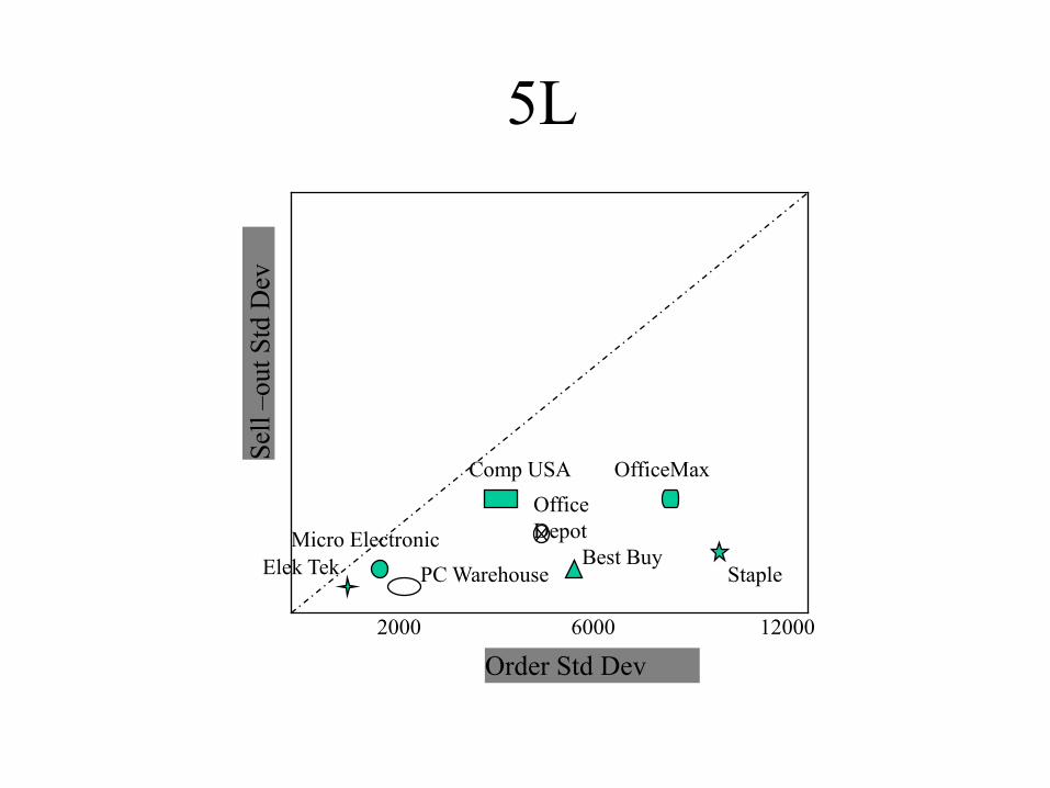
5L
Elek Tek
Micro Electronic
PC Warehouse
Comp USA
Office
Depot
Best Buy
OfficeMax
Staple
120002000 6000
Sel
l –o
ut
Std
Dev
Order Std Dev
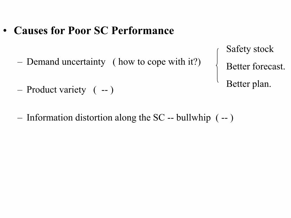
• Causes for Poor SC Performance
– Demand uncertainty ( how to cope with it?)
– Product variety ( -- )
– Information distortion along the SC -- bullwhip ( -- )
Safety stock
Better forecast.
Better plan.
Bullwhip EffectBullwhip Effect
Manufacturers Regional Local Local Local
Distributors Wholesalers Retailers Customers
Bullwhip effect: increased demand variability up the SC
Curses of Bullwhip EffectCurses of Bullwhip Effect
• Curses
–
–
–
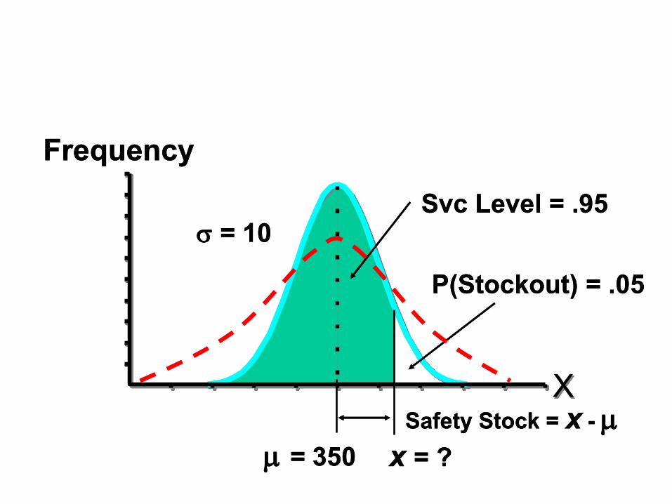
X
= 350= 350
Svc Level = .95Svc Level = .95
P(Stockout) = .05P(Stockout) = .05
FrequencyFrequency
xx = ?= ?
= 10= 10
Safety Stock = Safety Stock = xx --
Curses of Bullwhip EffectCurses of Bullwhip Effect
• Curses
– Inventory out of control
– Customer service degradation
– Misguided capacity planning (W/H, staffing, etc)
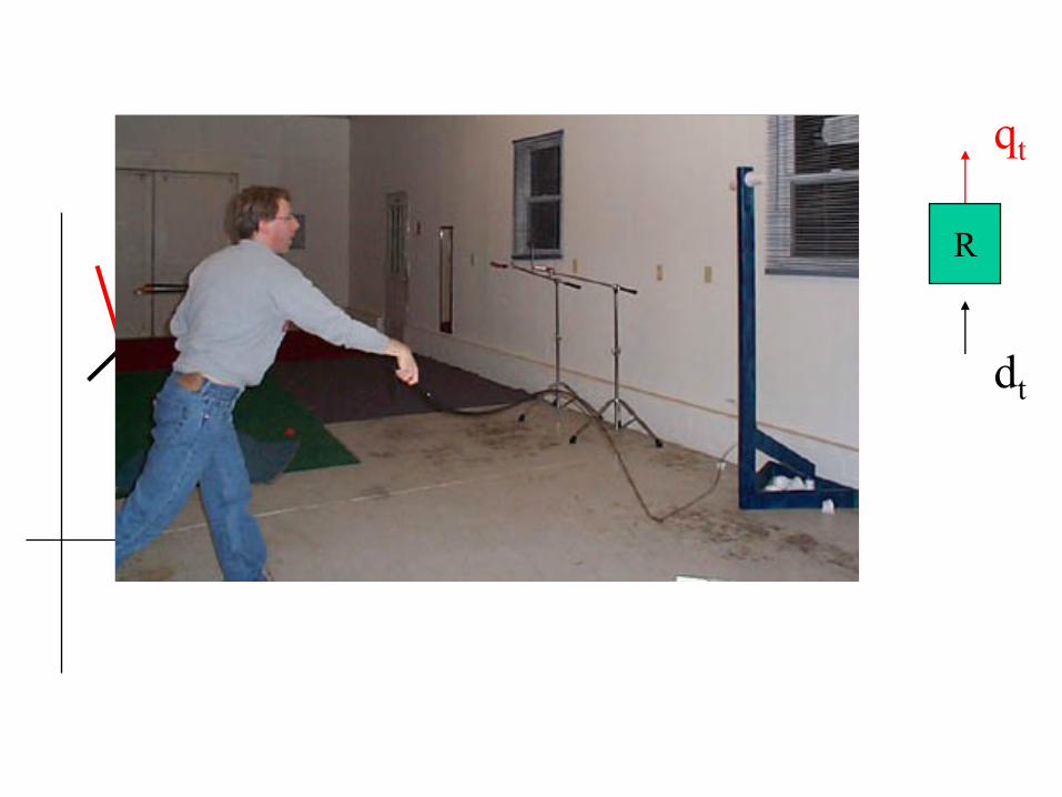
R
dt
qt
dt
qt
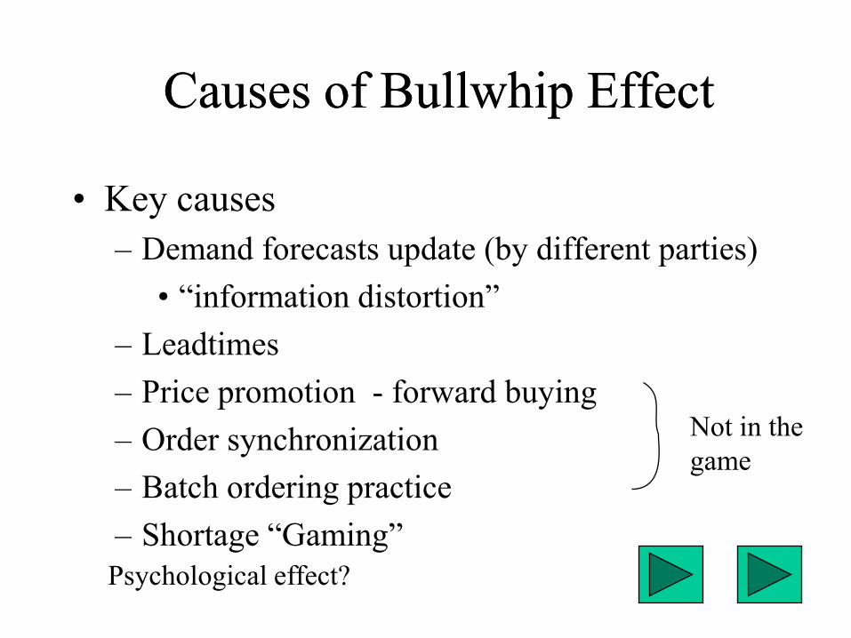
Causes of Bullwhip EffectCauses of Bullwhip Effect
• Key causes
– Demand forecasts update (by different parties)
• “information distortion”
– Leadtimes
– Price promotion - forward buying
– Order synchronization
– Batch ordering practice
– Shortage “Gaming”
Not in the
game
Psychological effect?
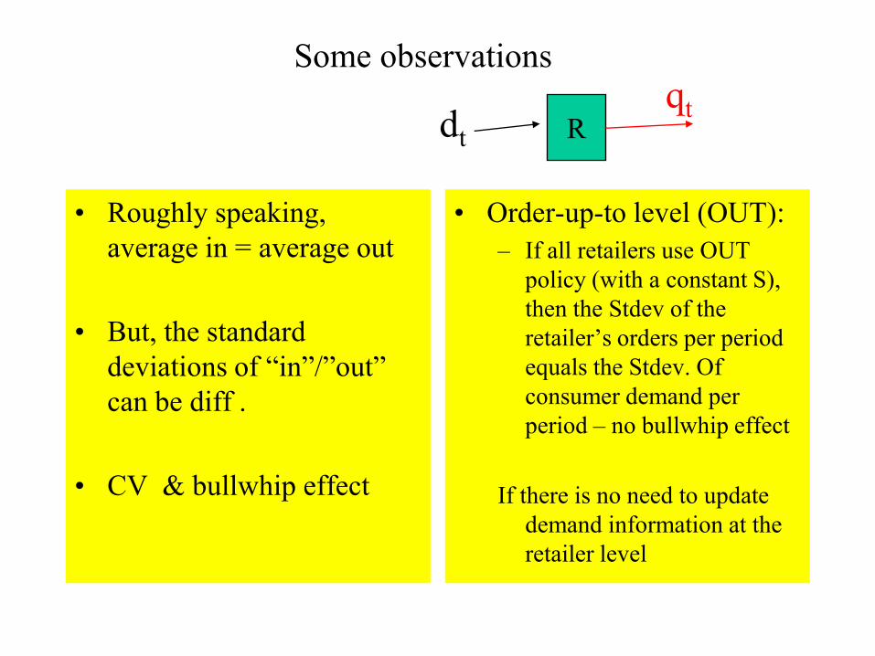
Some observations
• Roughly speaking,
average in = average out
• But, the standard
deviations of “in”/”out”
can be diff .
• CV & bullwhip effect
• Order-up-to level (OUT):
– If all retailers use OUT
policy (with a constant S),
then the Stdev of the
retailer’s orders per period
equals the Stdev. Of
consumer demand per
period – no bullwhip effect
If there is no need to update
demand information at the
retailer level
Rdt
qt
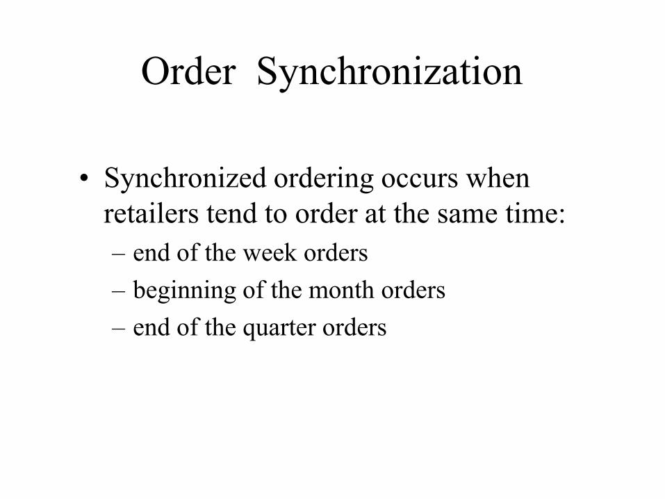
Order Synchronization
• Synchronized ordering occurs when
retailers tend to order at the same time:
– end of the week orders
– beginning of the month orders
– end of the quarter orders
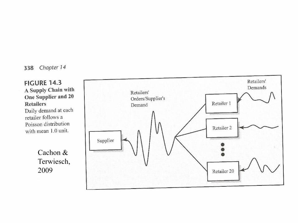
Cachon &
Terwiesch,
2009
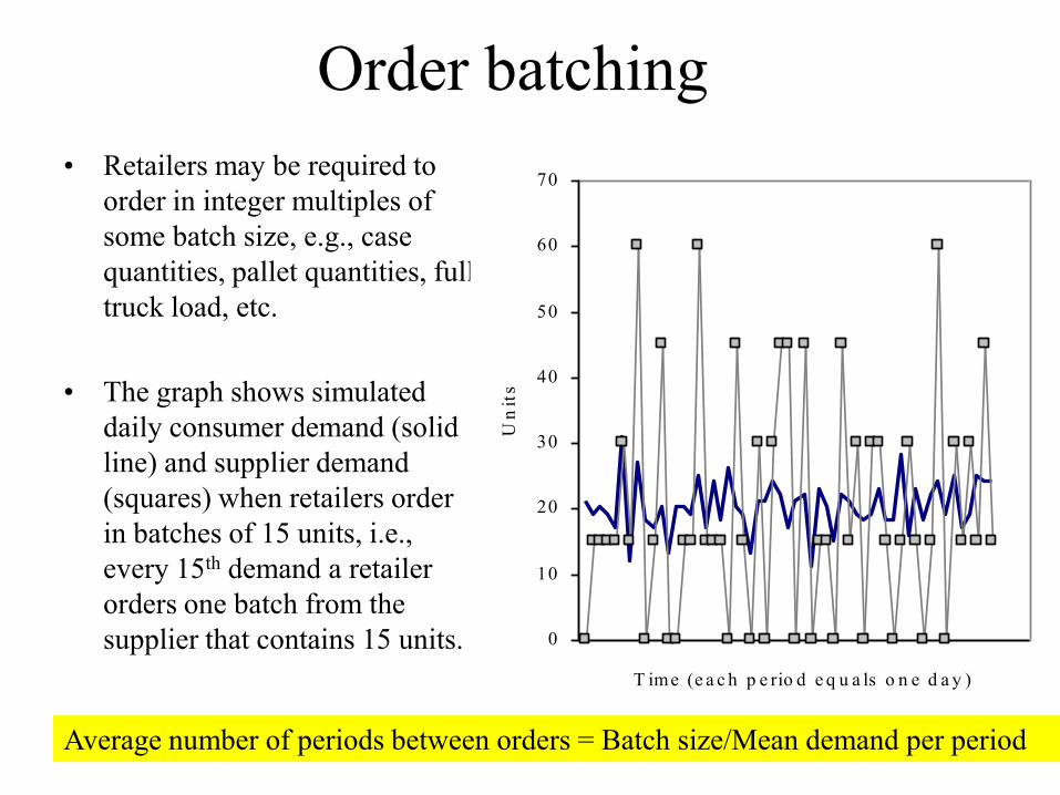
Order batching
• Retailers may be required to
order in integer multiples of
some batch size, e.g., case
quantities, pallet quantities, full
truck load, etc.
• The graph shows simulated
daily consumer demand (solid
line) and supplier demand
(squares) when retailers order
in batches of 15 units, i.e.,
every 15th demand a retailer
orders one batch from the
supplier that contains 15 units. 0
10
20
30
40
50
60
70
T ime (e a c h p e rio d e q u a ls o n e d a y )
Un
its
Average number of periods between orders = Batch size/Mean demand per period
• Smaller min order quantity (lower Q), so retailers
order more frequently
• Unsynchronize retailer order intervals
– Retailers may order every T periods
– Min batch size Q=1, so no min order Q restriction
– Retailers are placed on balanced schedules s.t. average
demand per period is held constant
• e.g., 100 identical retailers and T=5 implies 20
retailers may order each period
Order batching solutions
Trade Promotion Trade Promotion
• Why trade promotion?
• Consequences of trade promotion?
Forward Buying
Hey, I am offering
a discount x%
if u will buy in
(greater)bulk
OK! Triple the
qty I usually order!
I can try and sell
some at a promotion
and keep the rest and sell
at the regular price next time
Earn & save money!
Why big orders cause problem in this case?
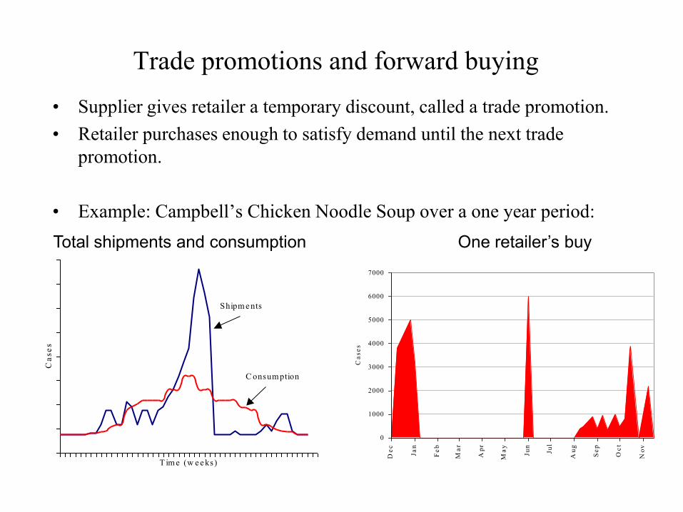
Trade promotions and forward buying
• Supplier gives retailer a temporary discount, called a trade promotion.
• Retailer purchases enough to satisfy demand until the next trade
promotion.
• Example: Campbell’s Chicken Noodle Soup over a one year period:
One retailer’s buy
T im e (w e e ks)
Ca
se
s
Shipm e nts
C onsum ption
0
1000
2000
3000
4000
5000
6000
7000
De
c
Ja
n
Fe
b
Ma
r
Ap
r
Ma
y
Ju
n
Ju
l
Au
g
Se
p
Oc
t
No
v
Ca
se
s
Total shipments and consumption
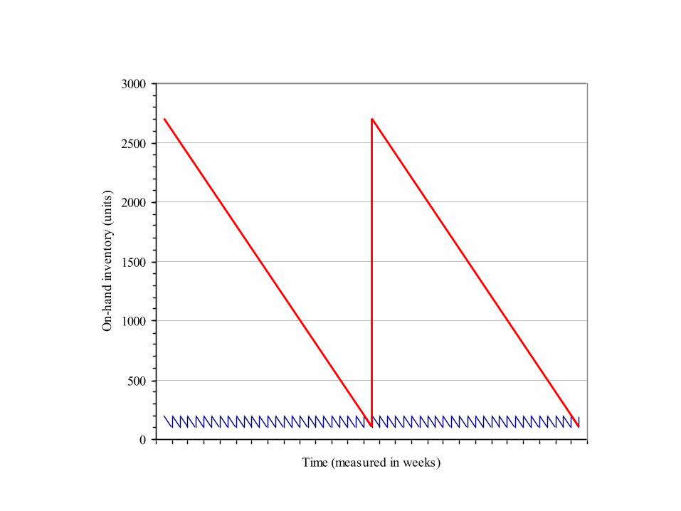
0
500
1000
1500
2000
2500
3000
Time (measured in weeks)
On
-han
d in
ven
tory
(u
nit
s)
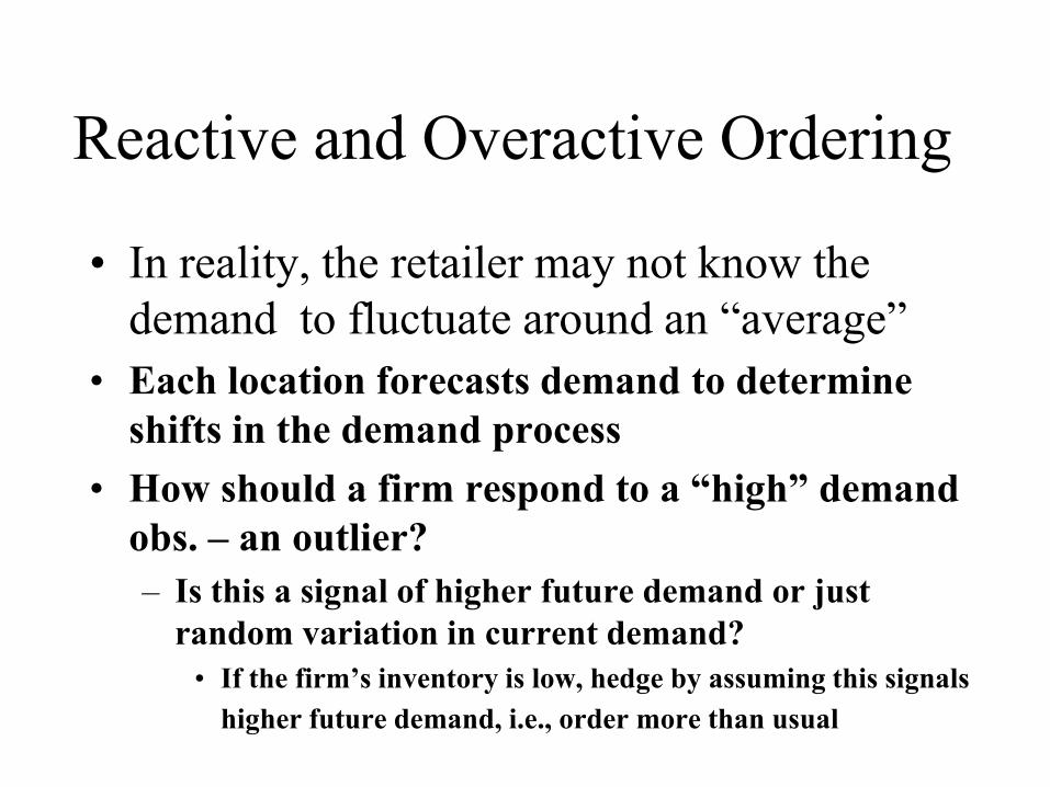
Reactive and Overactive Ordering
• In reality, the retailer may not know the
demand to fluctuate around an “average”
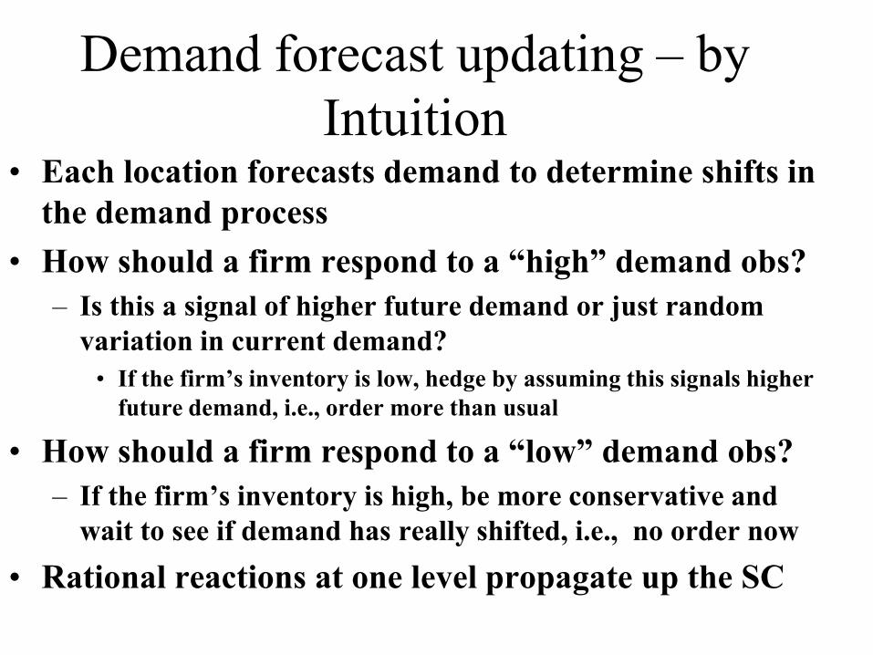
• Each location forecasts demand to determine
shifts in the demand process
• How should a firm respond to a “high” demand
obs. – an outlier?
– Is this a signal of higher future demand or just
random variation in current demand?
• If the firm’s inventory is low, hedge by assuming this signals
higher future demand, i.e., order more than usual
• Each location forecasts demand to determine shifts in
the demand process
• How should a firm respond to a “high” demand obs?
– Is this a signal of higher future demand or just random
variation in current demand?
• If the firm’s inventory is low, hedge by assuming this signals higher
future demand, i.e., order more than usual
• How should a firm respond to a “low” demand obs?
– If the firm’s inventory is high, be more conservative and
wait to see if demand has really shifted, i.e., no order now
• Rational reactions at one level propagate up the SC
Demand forecast updating – by
Intuition
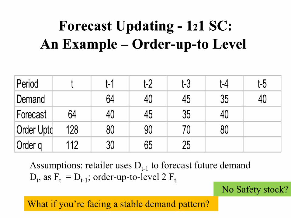
Forecast Updating - 121 SC:
An Example – Order-up-to Level
Forecast Updating - 121 SC:
An Example – Order-up-to Level
Period t t-1 t-2 t-3 t-4 t-5
Demand 64 40 45 35 40
Forecast 64 40 45 35 40
Order Upto 128 80 90 70 80
Order q 112 30 65 25
Assumptions: retailer uses Dt-1 to forecast future demand
Dt, as Ft = Dt-1; order-up-to-level 2 Ft.
No Safety stock?
What if you’re facing a stable demand pattern?
Impact of Forecasting on BEImpact of Forecasting on BE
• The BE is due, in part, to the need to forecast
demand & hold safety stock
• Moving ave and exponential smoothing are “bad”
• The fancier the method, the worse the BE
• Smoother demand forecasts can reduce the
bullwhip effect (MA & ES methods)
• The longer the leadtime, the higher the BE
• Centralised information sig reduces the BE
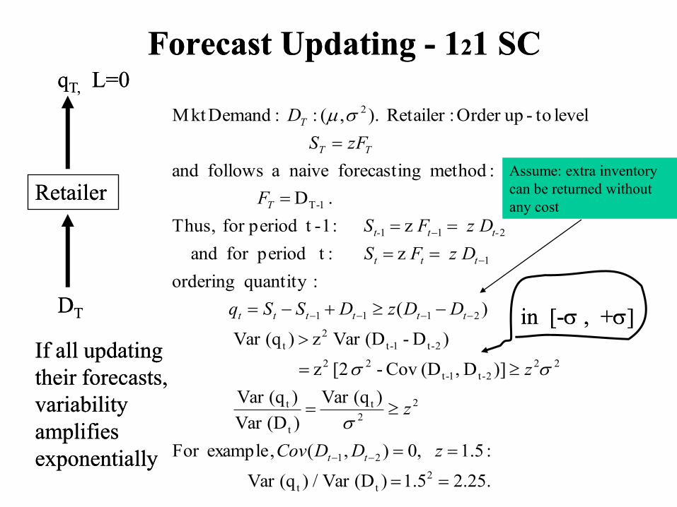
Forecast Updating - 121 SCForecast Updating - 121 SC
.25.21.5 )(DVar / )(qVar
:5.1 ,0),(,exampleFor
)(qVar
)(DVar
)(qVar
)]D ,(D Cov - [2 z
)D - (DVar z )(qVar
)(
:quantity ordering
z : tperiodfor and
z :1- tperiodfor Thus,
. D
:method gforecastin naive a follows and
level to-upOrder :Retailer ).,(: :DemandMkt
2
tt
21
2
2
t
t
t
22
2-t1-t
22
2-t1-t
2
t
2111
1
211
1-T
2
zDDCov
z
z
DDzDSSq
z DFS
z DF S
F
zFS
D
tt
tttttt
ttt
t-tt-
T
TT
T
RetailerRetailer
DDTT
qqT, T, L=0L=0
If all updating If all updating
their forecasts, their forecasts,
variability variability
amplifies amplifies
exponentiallyexponentially
in [in [-- , +, +]]
Assume: extra inventory
can be returned without
any cost
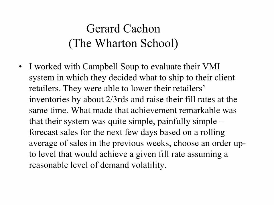
Gerard Cachon
(The Wharton School)
• I worked with Campbell Soup to evaluate their VMI
system in which they decided what to ship to their client
retailers. They were able to lower their retailers’
inventories by about 2/3rds and raise their fill rates at the
same time. What made that achievement remarkable was
that their system was quite simple, painfully simple –
forecast sales for the next few days based on a rolling
average of sales in the previous weeks, choose an order up-
to level that would achieve a given fill rate assuming a
reasonable level of demand volatility.
Avoiding Demand Forecast Updates
• Channel Alignment
– VMI - vendor managed inventory scheme
– Consumer direct
– Discount for information sharing, including
plan of promotion activities
• Operational Efficiency
– Leadtime reduction
– Echelon-based inventory control
Avoiding Demand Forecast Updates
• BE resulted from the chain effect along the SC
– Repetitive multiple forecast updating
• Share demand information so that every one can
obs demand shifts without distortions:
– Demand forecasts should be based on final sales to
consumers
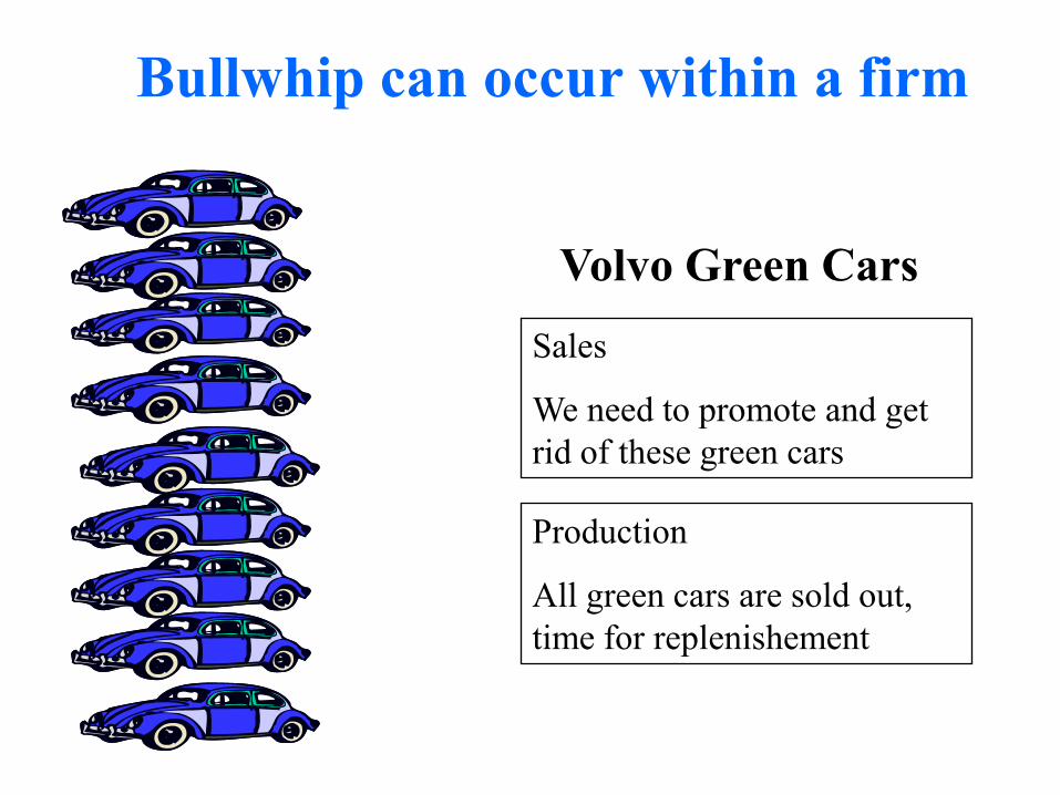
Bullwhip can occur within a firm
Sales
We need to promote and get
rid of these green cars
Production
All green cars are sold out,
time for replenishement
Volvo Green Cars

A Bigger Colour
Problem
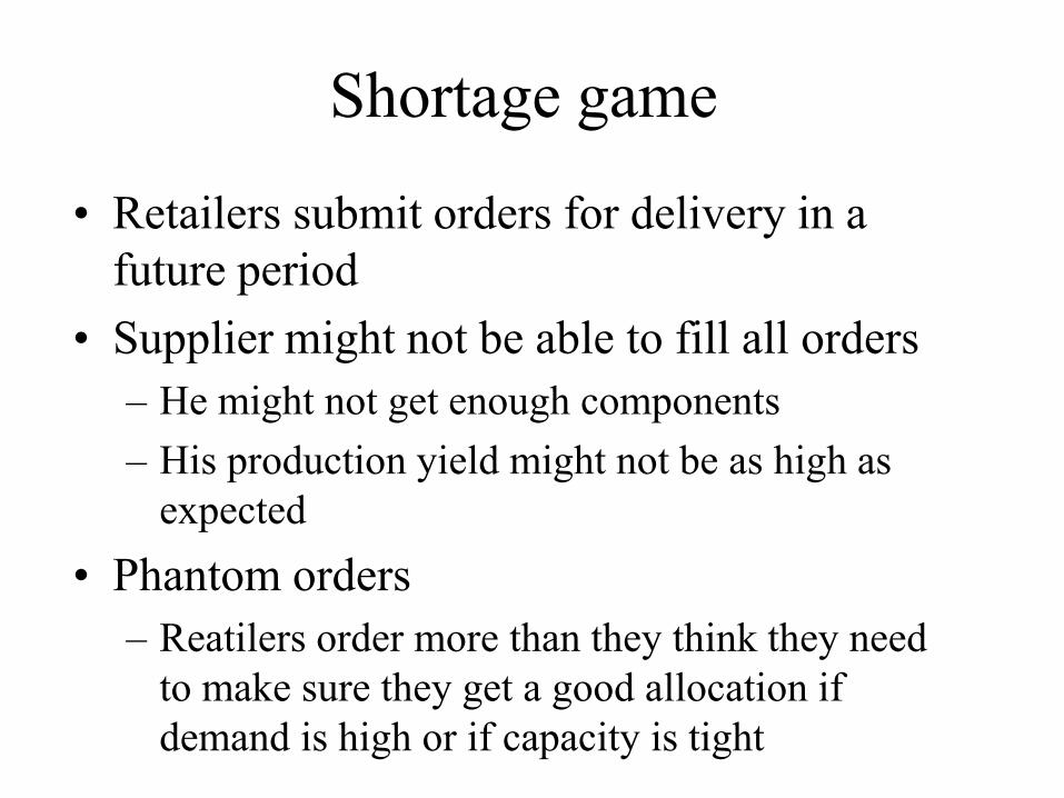
• Retailers submit orders for delivery in a
future period
• Supplier might not be able to fill all orders
– He might not get enough components
– His production yield might not be as high as
expected
• Phantom orders
– Reatilers order more than they think they need
to make sure they get a good allocation if
demand is high or if capacity is tight
Shortage game
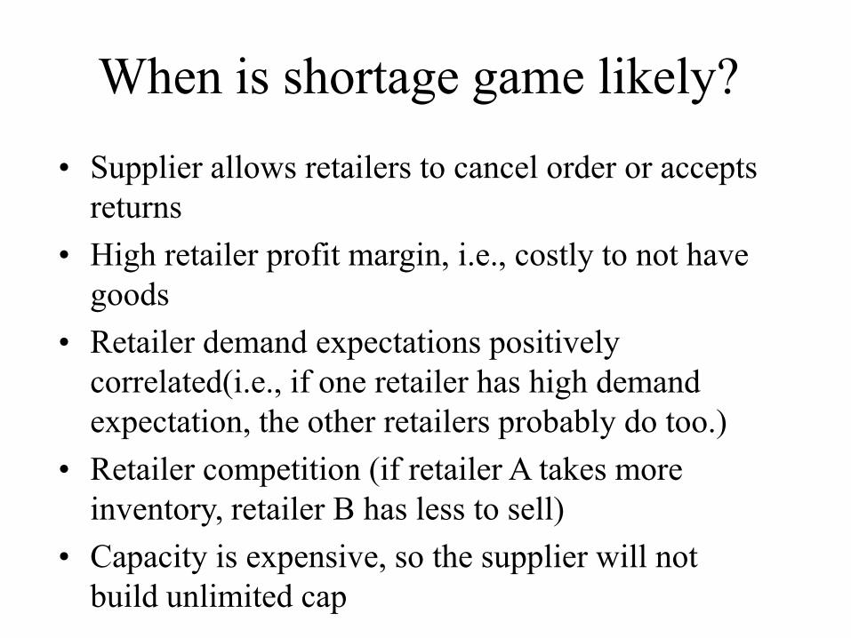
• Supplier allows retailers to cancel order or accepts
returns
• High retailer profit margin, i.e., costly to not have
goods
• Retailer demand expectations positively
correlated(i.e., if one retailer has high demand
expectation, the other retailers probably do too.)
• Retailer competition (if retailer A takes more
inventory, retailer B has less to sell)
• Capacity is expensive, so the supplier will not
build unlimited cap
When is shortage game likely?
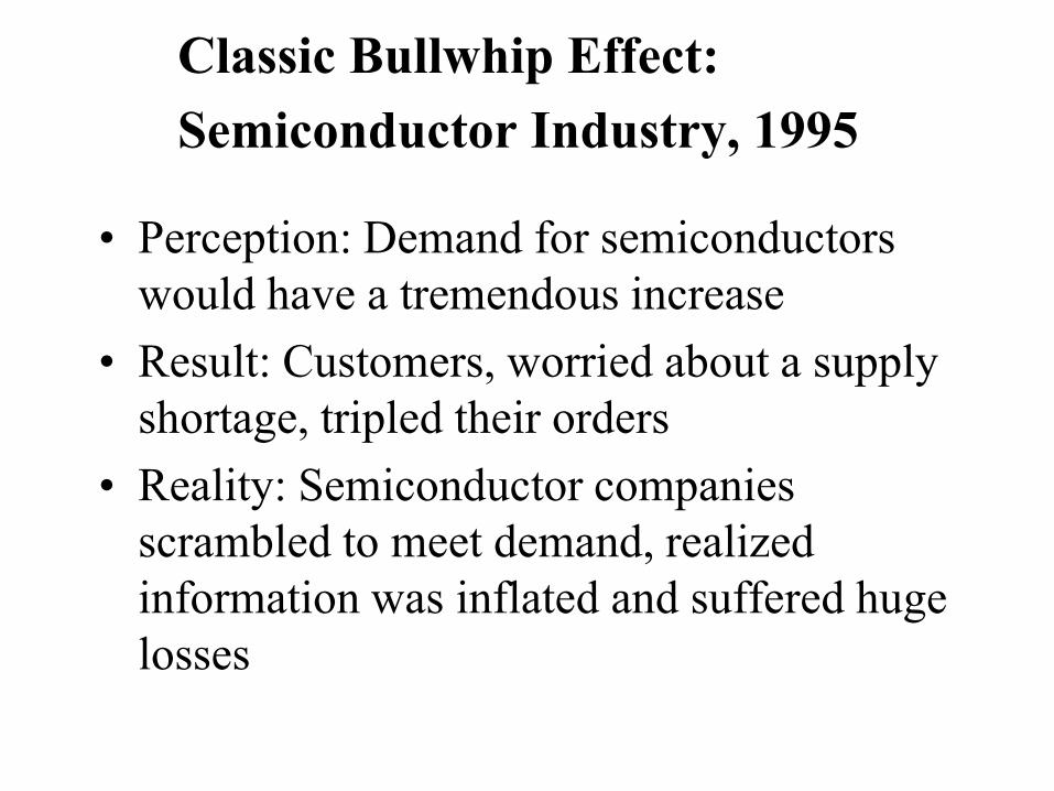
Classic Bullwhip Effect:
Semiconductor Industry, 1995
• Perception: Demand for semiconductors
would have a tremendous increase
• Result: Customers, worried about a supply
shortage, tripled their orders
• Reality: Semiconductor companies
scrambled to meet demand, realized
information was inflated and suffered huge
losses
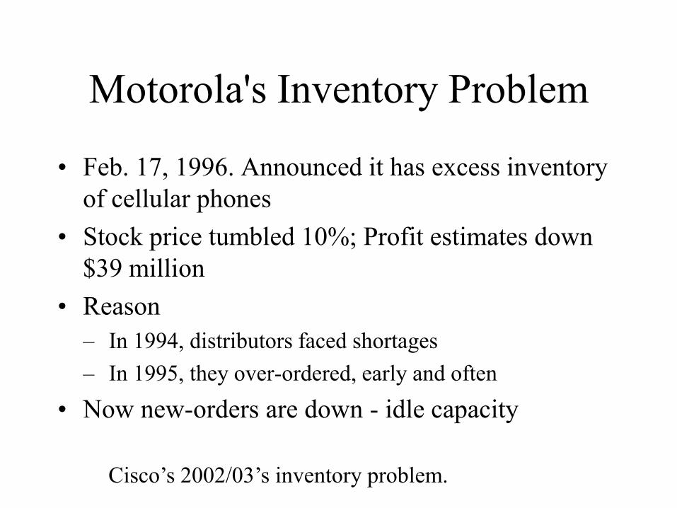
Motorola's Inventory Problem
• Feb. 17, 1996. Announced it has excess inventory
of cellular phones
• Stock price tumbled 10%; Profit estimates down
$39 million
• Reason
– In 1994, distributors faced shortages
– In 1995, they over-ordered, early and often
• Now new-orders are down - idle capacity
Cisco’s 2002/03’s inventory problem.
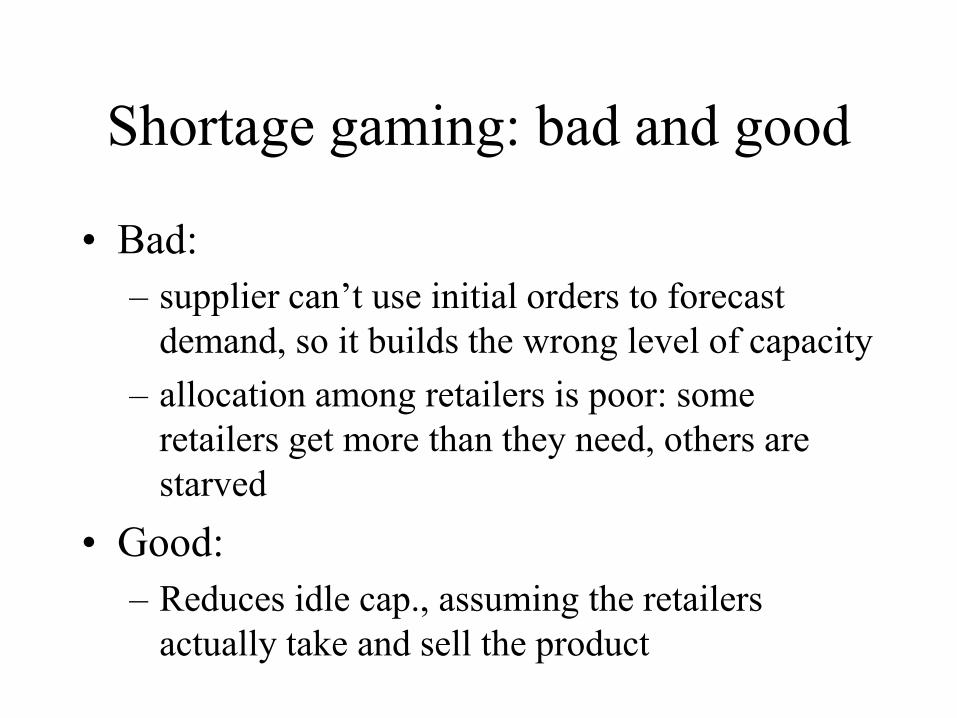
• Bad:
– supplier can’t use initial orders to forecast
demand, so it builds the wrong level of capacity
– allocation among retailers is poor: some
retailers get more than they need, others are
starved
• Good:
– Reduces idle cap., assuming the retailers
actually take and sell the product
Shortage gaming: bad and good
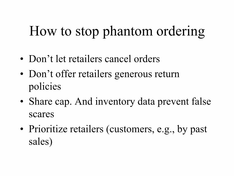
• Don’t let retailers cancel orders
• Don’t offer retailers generous return
policies
• Share cap. And inventory data prevent false
scares
• Prioritize retailers (customers, e.g., by past
sales)
How to stop phantom ordering
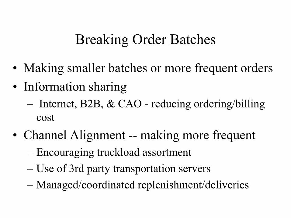
Breaking Order Batches
• Making smaller batches or more frequent orders
• Information sharing
– Internet, B2B, & CAO - reducing ordering/billing
cost
• Channel Alignment -- making more frequent
– Encouraging truckload assortment
– Use of 3rd party transportation servers
– Managed/coordinated replenishment/deliveries

![El Bullwhip Effect[1]- Yerlani](https://static.documents.pub/doc/80x56/577d29c31a28ab4e1ea7c468/el-bullwhip-effect1-yerlani.jpg)


