Page 1
Distinctive image features from scale-invariant keypoints. David G. Lowe, Int. Journal of Computer Vision, 60, 2
(2004), pp. 91-110
Presented by: Shalomi EldarBased (in part) on slides by Ofir Pele, Kirill Dyagilev and Ayelet
Dominitz
SIFTSIFTScale Invariant Feature Transform
Vision Topics Seminar 2009
[ ]c n[ ]c n[ ]c n
Page 2
2
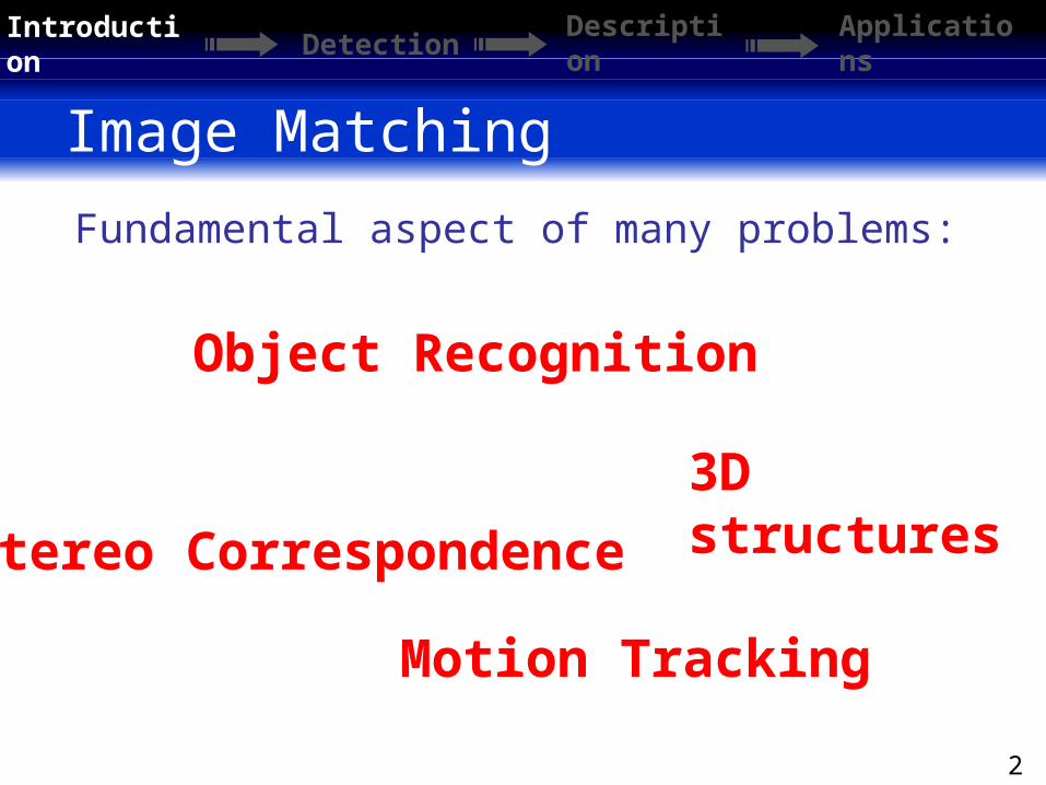
Image Matching
Introduction
Detection Description
Applications
Motion Tracking
Fundamental aspect of many problems:
Object Recognition
3D structuresStereo Correspondence
Page 3
3
Features Detection
Introduction
Detection Description
Applications
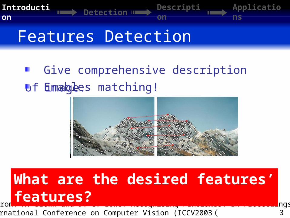
Give comprehensive description of
image.
Images from: M. Brown and D. G. Lowe. Recognising Panoramas. In Proceedings of the ) the International Conference on Computer Vision (ICCV2003
Enables matching!
What are the desired features’ features?
Page 4
4
Features’ Features
Introduction
Detection Description
Applications
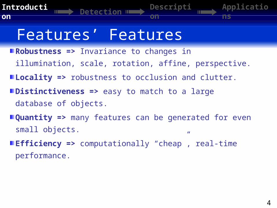
Robustness => Invariance to changes in
illumination, scale, rotation, affine, perspective.
Locality => robustness to occlusion and clutter.
Distinctiveness => easy to match to a large
database of objects.
Quantity => many features can be generated for
even small objects.
Efficiency => computationally “cheap”, real-time
performance.
Page 5
5
SIFT Algorithm
Introduction
Detection Description
Applications
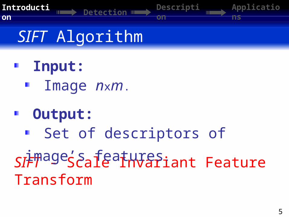
SIFT - Scale Invariant Feature Transform
Input: Image nxm.
Output: Set of descriptors of image’s
features.
Page 6
6
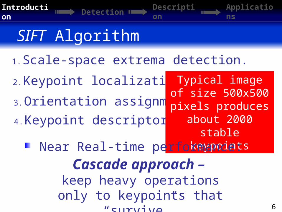
SIFT Algorithm
2. Keypoint localization.
1. Scale-space extrema detection.
3. Orientation assignment.
4. Keypoint descriptor.
Introduction
Detection Description
Applications
Typical image of size 500x500
pixels produces about 2000 stable
keypoints Near Real-time performance:
Cascade approach – keep heavy operations only to keypoints that “survive”.
Page 7
7
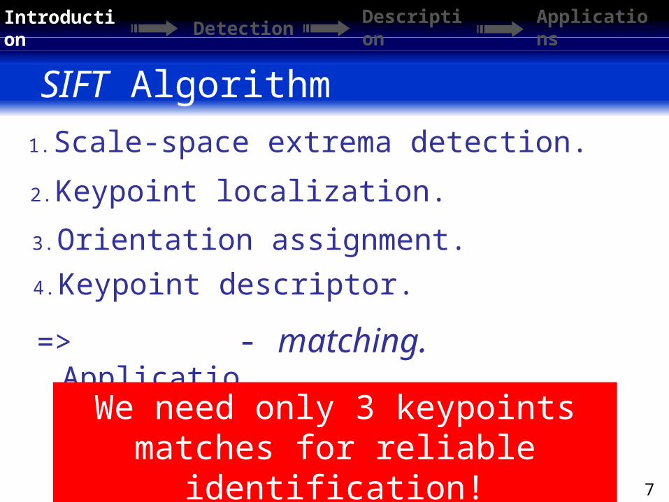
SIFT Algorithm
Introduction
Detection Description
Applications
2. Keypoint localization.
1. Scale-space extrema detection.
3. Orientation assignment.
4. Keypoint descriptor.
=> Application
- matching.
We need only 3 keypoints matches for reliable
identification!
Page 8
8
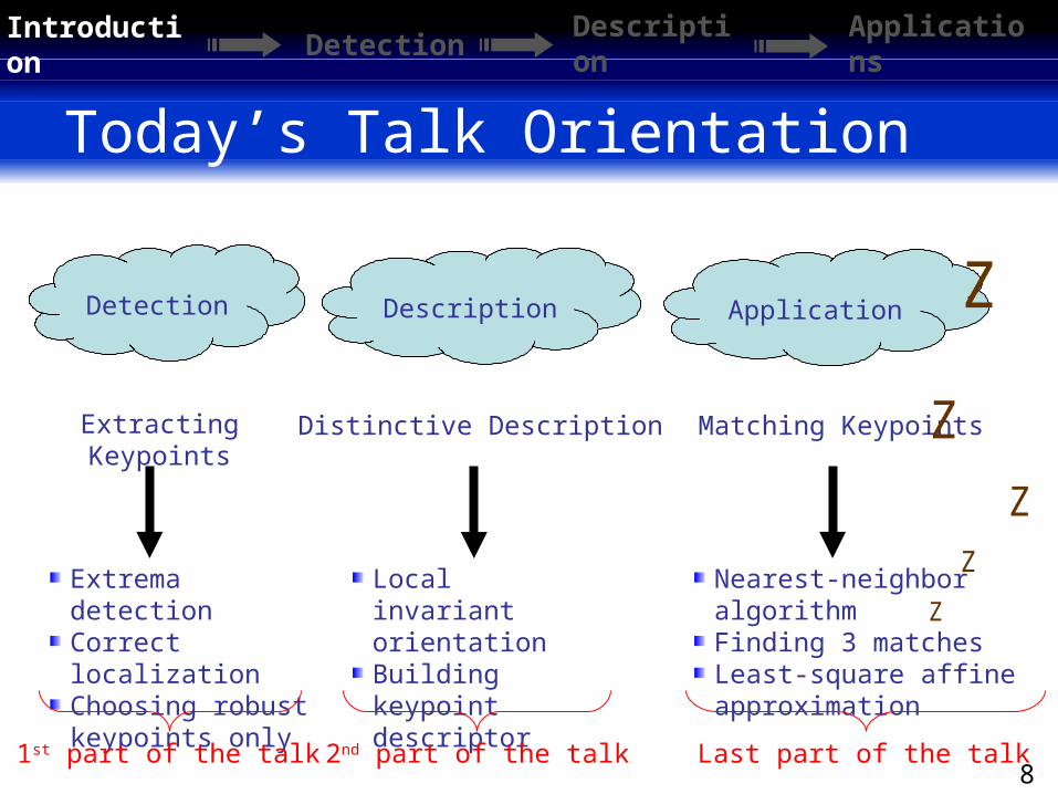
Today’s Talk Orientation
Extracting Keypoints
Distinctive Description Matching Keypoints
Extrema detectionCorrect localizationChoosing robust keypoints only
Local invariant orientationBuilding keypoint descriptor
Nearest-neighbor algorithmFinding 3 matchesLeast-square affine approximation
Detection Description Application
1st part of the talk 2nd part of the talk Last part of the talk
Z
Z
Z Z
Z
Introduction
Detection Description
Applications
Page 9
9
SIFT Algorithm
2. Keypoint localization.
1. Scale-space extrema detection.
3. Orientation assignment.
4. Keypoint descriptor.
Introduction
Detection Description
Applications
Collecting keypoint candidates…
Page 10
10
Introduction
Detection Description
Applications
Why Extrema?
We want to find points that give us information about the objects in the image.
We will represent the image in a way that gives us these edges as this representations extrema points.
The information about the objects is in the object’s edges.
Page 11
11
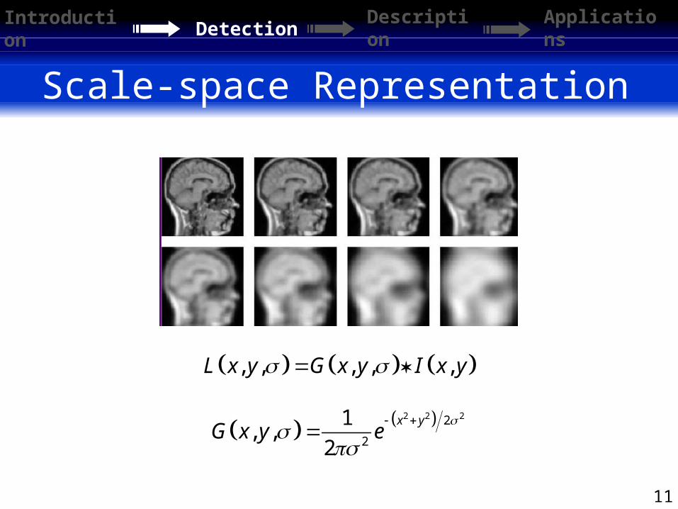
Scale-space Representation
Introduction
Detection Description
Applications
, , , , ,L x y G x y I x y
2 2 22
2
1, ,
2
x yG x y e
Page 12
12
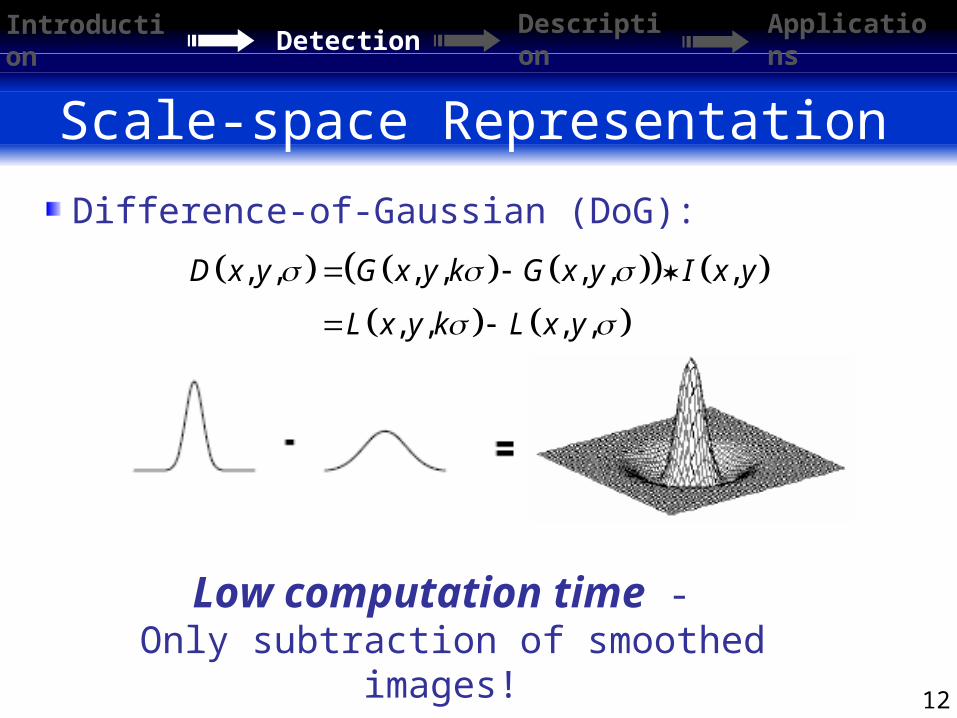
Low computation time - Only subtraction of smoothed
images!
Introduction
Detection Description
Applications
Scale-space Representation
, , , , , , ,
, , , ,
D x y G x y k G x y I x y
L x y k L x y
Difference-of-Gaussian (DoG):
Page 13
13
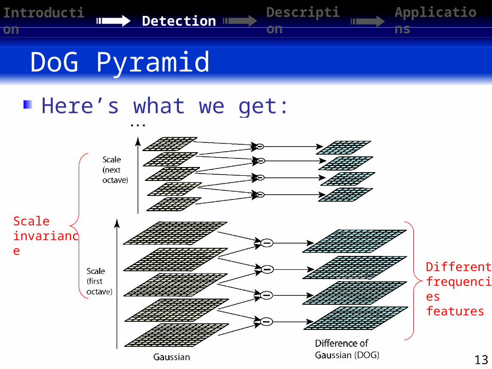
Here’s what we get:
Introduction
Detection Description
Applications
DoG Pyramid
Different frequencies features
Scale invariance
Page 14
14
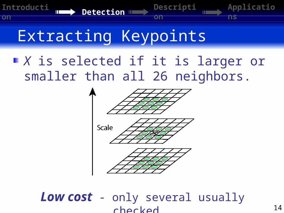
X is selected if it is larger or smaller than all 26 neighbors.
Introduction
Detection Description
Applications
Extracting Keypoints
Low cost - only several usually checked.
Page 15
15
Extrema detection product:
Introduction
Detection Description
Applications
Extracting Keypoints
Not all of them are good…
233x189 image => 832 DoG Keypoints.Each Keypoint is represented as . , ,x y
Page 16
16
Problematic Keypoints
Introduction
Detection Description
Applications
Inaccurate localization (due to scaling and sampling).
Low contrast - sensitive to noise.Strong edge responses.
Page 17
17
SIFT Algorithm
2. Keypoint localization.
1. Scale-space extrema detection.
3. Orientation assignment.
4. Keypoint descriptor.Filtering Keypoints…
Introduction
Detection Description
Applications
Page 18
18
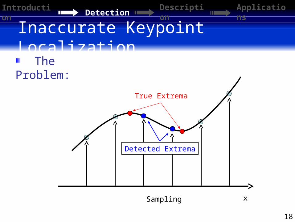
Inaccurate Keypoint Localization
Introduction
Detection Description
Applications
xSampling
Detected Extrema
True Extrema
The Problem:
Page 19
19
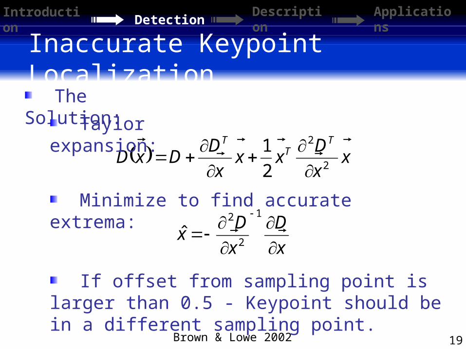
Inaccurate Keypoint Localization
Introduction
Detection Description
Applications
The Solution:
xx
Dxx
x
DDxD
TT
T
2
2
2
1
Taylor expansion:
Minimize to find accurate extrema:
x
D
x
Dx
1
2
2
ˆ
Brown & Lowe 2002
If offset from sampling point is larger than 0.5 - Keypoint should be in a different sampling point.
Page 20
20
Low Contrast Keypoints
Introduction
Detection Description
Applications
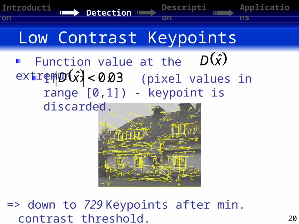
Function value at the extremun - xD ˆIf (pixel values in range [0,1]) - keypoint is discarded.
03.0ˆ xD
=> down to 729 Keypoints after min. contrast threshold.
Page 21
21
Eliminating Edge Responses
Introduction
Detection Description
Applications
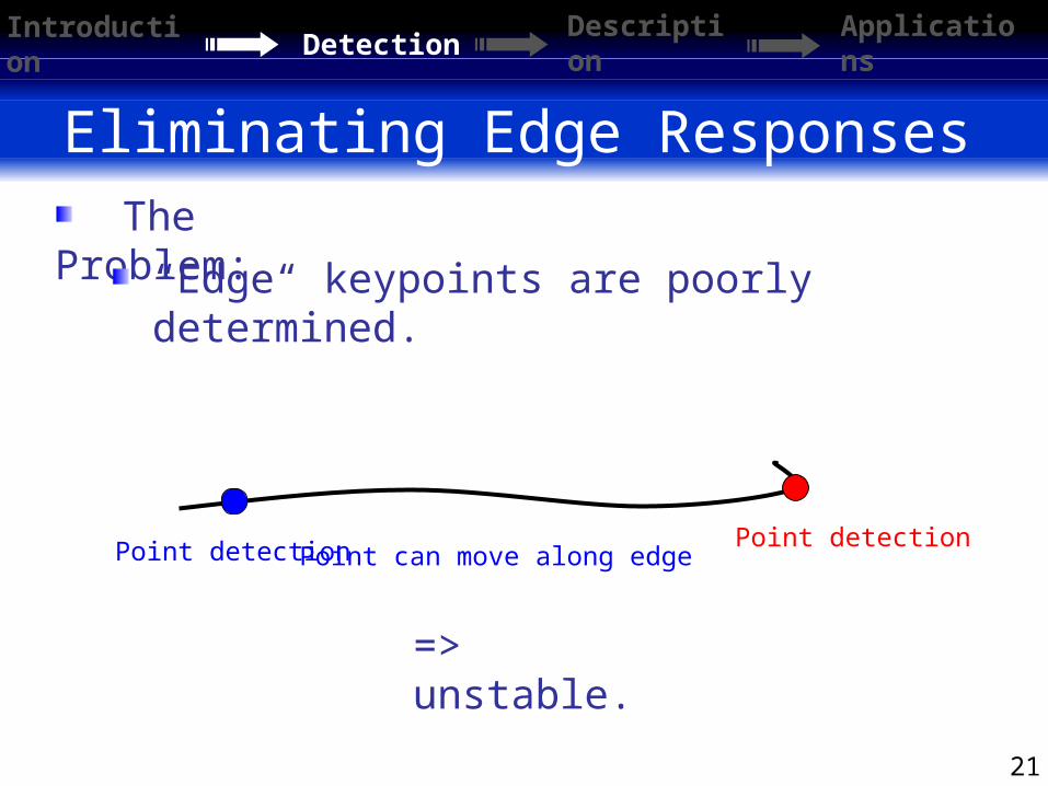
The Problem:“Edge“ keypoints are poorly
determined.
Point can move along edgePoint detection Point detection
=> unstable.
Page 22
22
Eliminating Edge Responses
Introduction
Detection Description
Applications
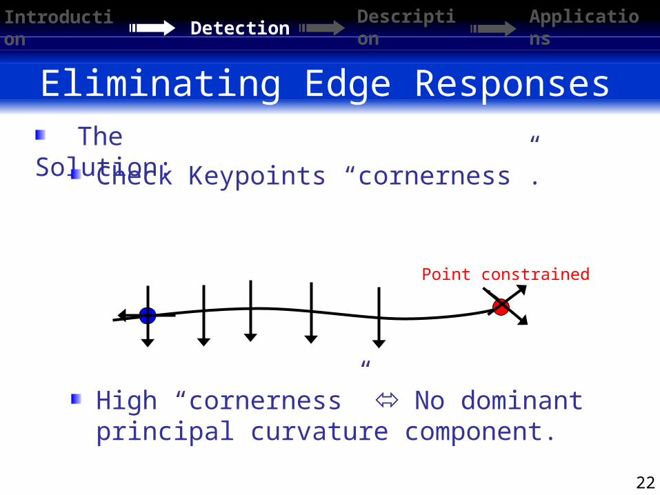
The Solution:Check Keypoints “cornerness”.
Point constrained
High “cornerness” No dominant principal curvature component.
Page 23
23
Finding “Cornerness”
Introduction
Detection Description
Applications
xx xy
xy yy
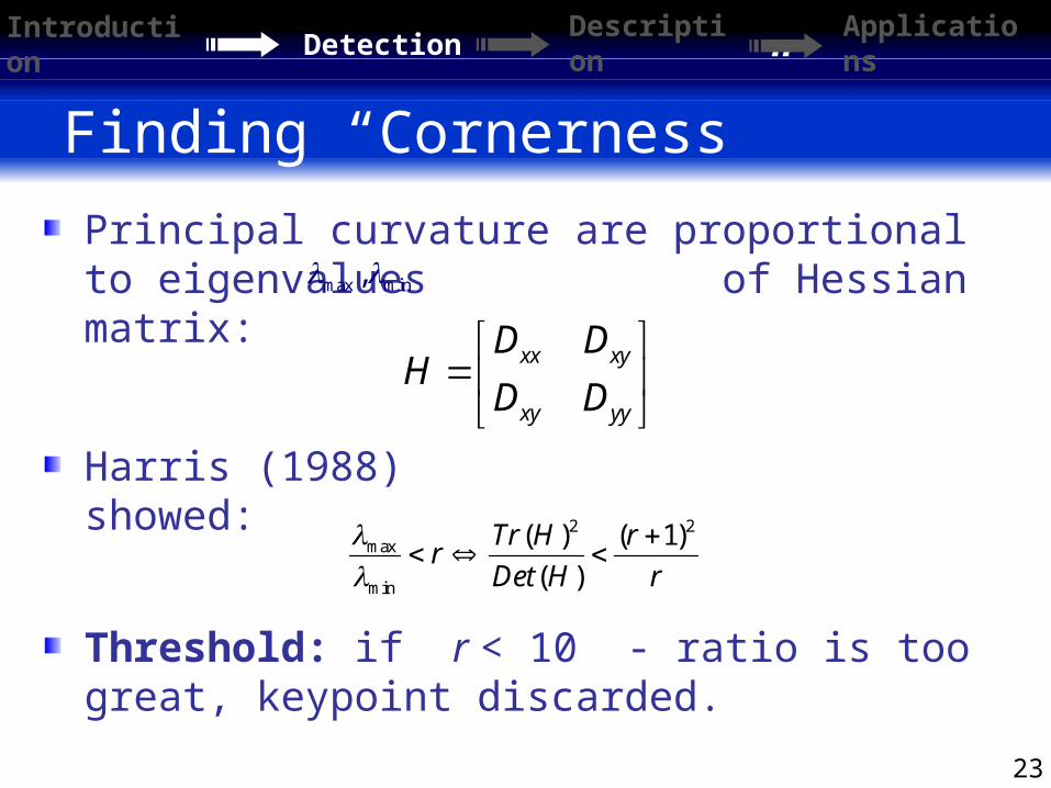
D DH
D D
Principal curvature are proportional to eigenvalues of Hessian matrix:max min,
2 2max
min
) ) ) 1)
) )
Tr H rr
Det H r
Harris (1988) showed:
Threshold: if r < 10 - ratio is too great, keypoint discarded.
Page 24
24
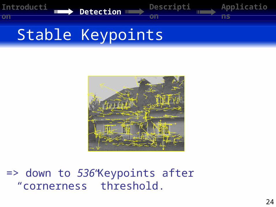
Stable Keypoints
Introduction
Detection Description
Applications
=> down to 536 Keypoints after “cornerness” threshold.
Page 25
25
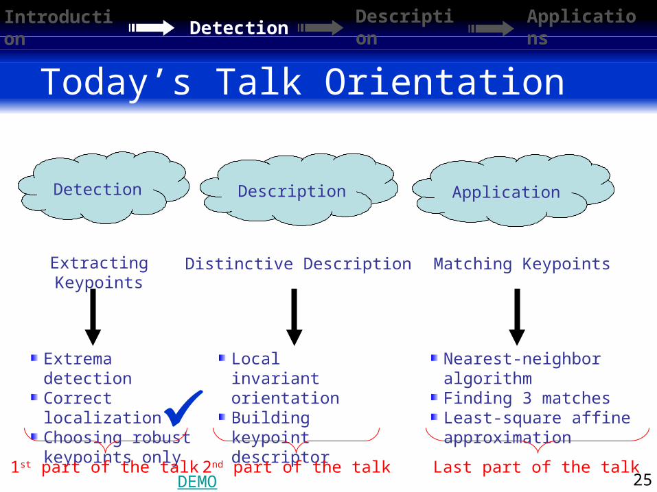
Today’s Talk Orientation
Extracting Keypoints
Distinctive Description Matching Keypoints
Extrema detectionCorrect localizationChoosing robust keypoints only
Local invariant orientationBuilding keypoint descriptor
Nearest-neighbor algorithmFinding 3 matchesLeast-square affine approximation
Detection Description Application
1st part of the talk 2nd part of the talk Last part of the talk
Introduction
Detection Description
Applications
DEMO
Page 26
26
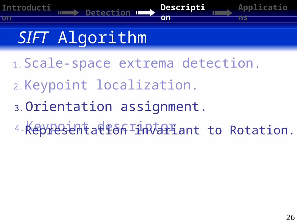
SIFT Algorithm
2. Keypoint localization.
1. Scale-space extrema detection.
3. Orientation assignment.
4. Keypoint descriptor.Representation invariant to Rotation.
Introduction
Detection Description
Applications
Page 27
27
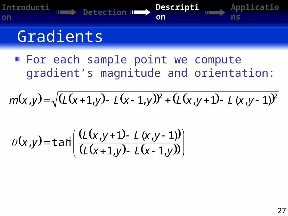
Gradients
Introduction
Detection Description
Applications
yxLyxL
yxLyxLyx
yxLyxLyxLyxLyxm
,1,1
)1,)1,tan,
)1,)1,,1,1,
1
22
For each sample point we compute gradient’s magnitude and orientation:
Page 28
28
Keypoints Orientation
Introduction
Detection Description
Applications
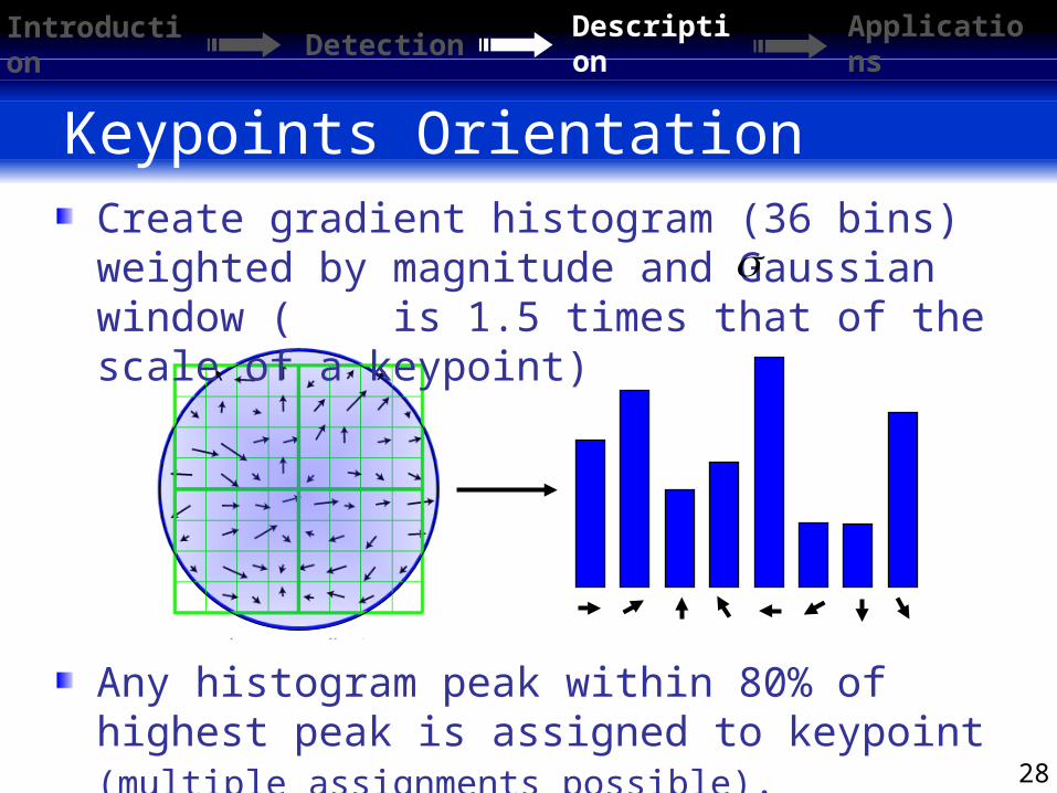
Create gradient histogram (36 bins) weighted by magnitude and Gaussian window ( is 1.5 times that of the scale of a keypoint)
Any histogram peak within 80% of highest peak is assigned to keypoint (multiple assignments possible).
Page 29
29
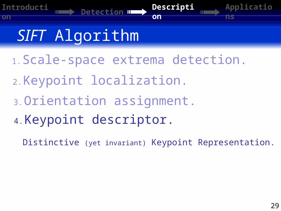
SIFT Algorithm
2. Keypoint localization.
1. Scale-space extrema detection.
3. Orientation assignment.
4. Keypoint descriptor.
Distinctive (yet invariant) Keypoint Representation.
Introduction
Detection Description
Applications
Page 30
30
What do we have (and what don’t)
For each Keypoint we have assigned location, scale and orientation.Provides invariance to these parameters.
Introduction
Detection Description
Applications
Do:
Sufficient distinctiveness.
Invariance to other parameters, such as 3D viewpoint and change of illumination.
Don’t:
Page 31
31
Keypoint Descriptor
Introduction
Detection Description
Applications
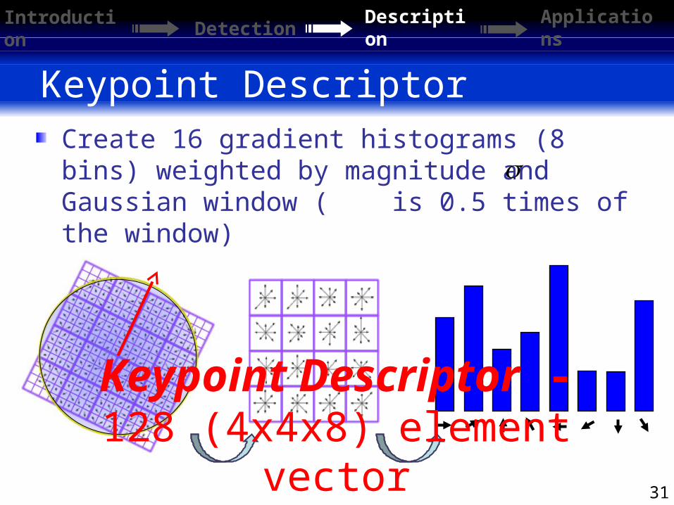
Create 16 gradient histograms (8 bins) weighted by magnitude and Gaussian window ( is 0.5 times of the window)
Keypoint Descriptor -
128 (4x4x8) element vector
Page 32
32
Change of Illumination
Introduction
Detection Description
Applications
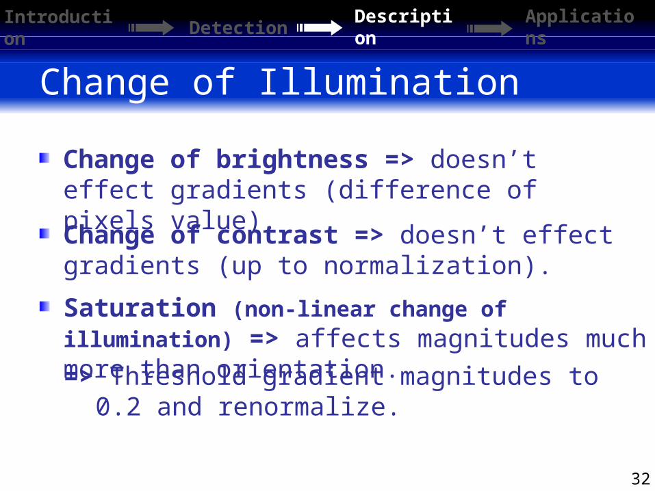
Change of brightness => doesn’t effect gradients (difference of pixels value).
Change of contrast => doesn’t effect gradients (up to normalization).
Saturation (non-linear change of illumination) => affects magnitudes much more than orientation.=> Threshold gradient magnitudes to 0.2
and renormalize.
Page 33
33
Today’s Talk Orientation
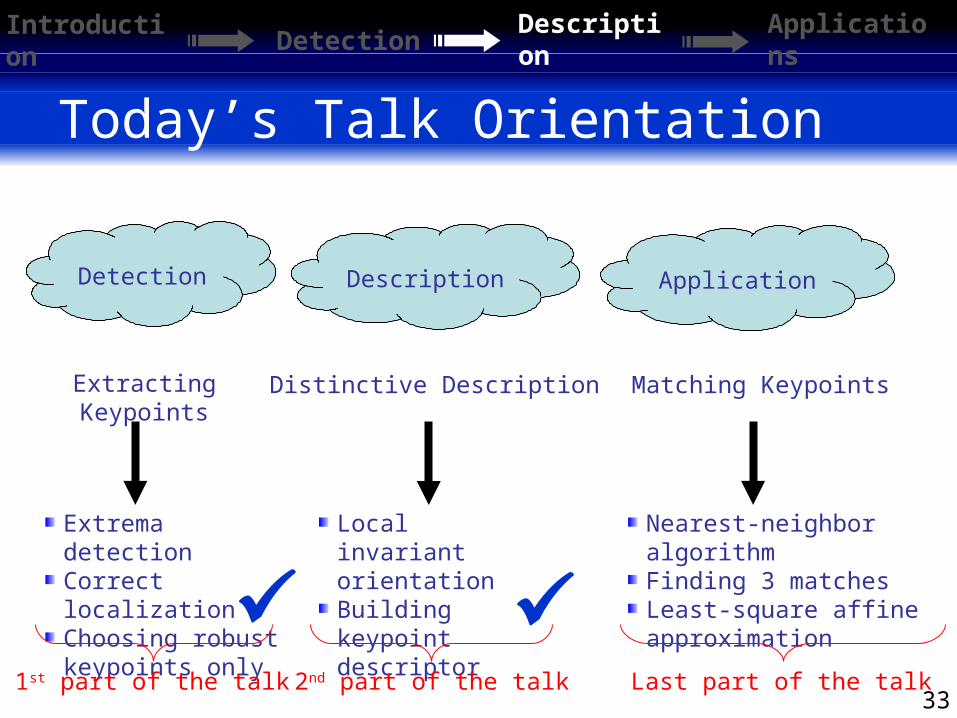
Extracting Keypoints
Distinctive Description Matching Keypoints
Extrema detectionCorrect localizationChoosing robust keypoints only
Local invariant orientationBuilding keypoint descriptor
Nearest-neighbor algorithmFinding 3 matchesLeast-square affine approximation
Detection Description Application
1st part of the talk 2nd part of the talk Last part of the talk
Introduction
Detection Description
Applications
Page 34
34
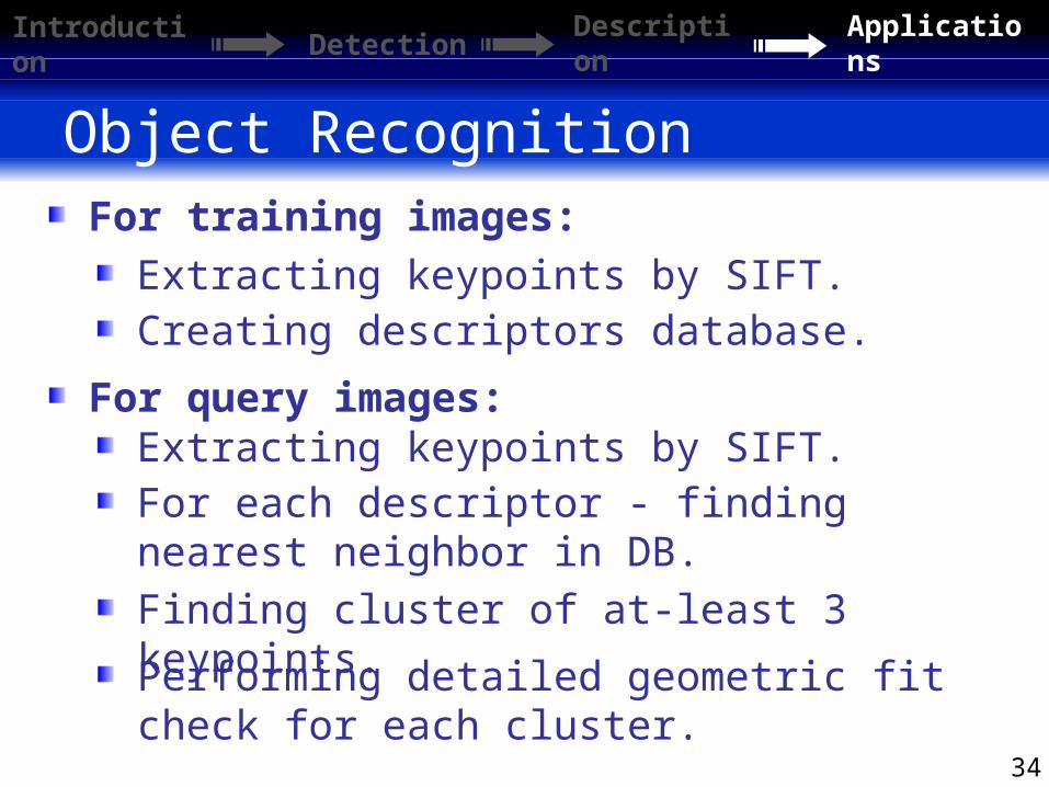
Object RecognitionFor training images:
Extracting keypoints by SIFT.Creating descriptors database.
Performing detailed geometric fit check for each cluster.
Introduction
Detection Description
Applications
For query images:Extracting keypoints by SIFT.For each descriptor - finding nearest neighbor in DB. Finding cluster of at-least 3 keypoints.
Page 35
35
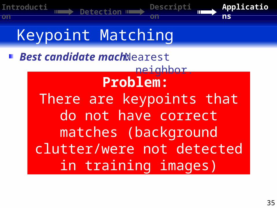
Keypoint MatchingBest candidate mach:
Introduction
Detection Description
Applications
Problem: There are keypoints that do not have correct matches
(background clutter/were not detected in training images)
Nearest neighbor.
Page 36
36
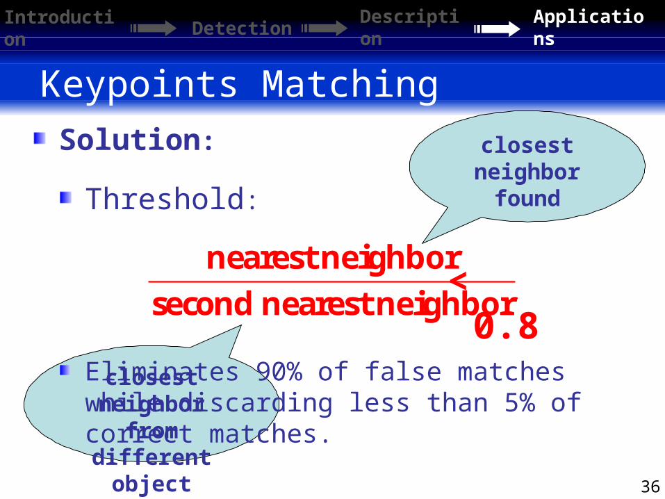
Keypoints MatchingSolution:
Introduction
Detection Description
Applications
nearest neighborsecond nearest neighbor
closest neighbor
found
closest neighbor
from different
object
Threshold:
< 0.8
Eliminates 90% of false matches while discarding less than 5% of correct matches.
Page 37
37
No good algorithm for high dimensional spaces.
Finding Nearest Neighbor
Introduction
Detection Description
Applications
=> Use Best-Bin-First (BBF) algorithm (Beis and Lowe, 1997).
=> Returns closest neighbor with high probability.
Low cost - cutting off search after checking specific number of
candidates. Good enough - we only need to show 0.8 ratio between first and
second neighbor.
Page 38
38
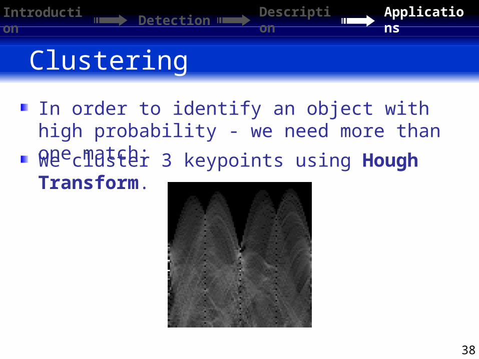
Clustering
We cluster 3 keypoints using Hough Transform.
In order to identify an object with high probability - we need more than one match:
Introduction
Detection Description
Applications
Page 39
39
Geometric VerificationHough Transform found clusters of keypoints.
Introduction
Detection Description
Applications
We would like to verify that these points do match geometrically to trained image.
In order to do that we use least-squares approach to find affine transformation from training image to query image.
Now we can be pretty sure we got the right object!
Page 40
40
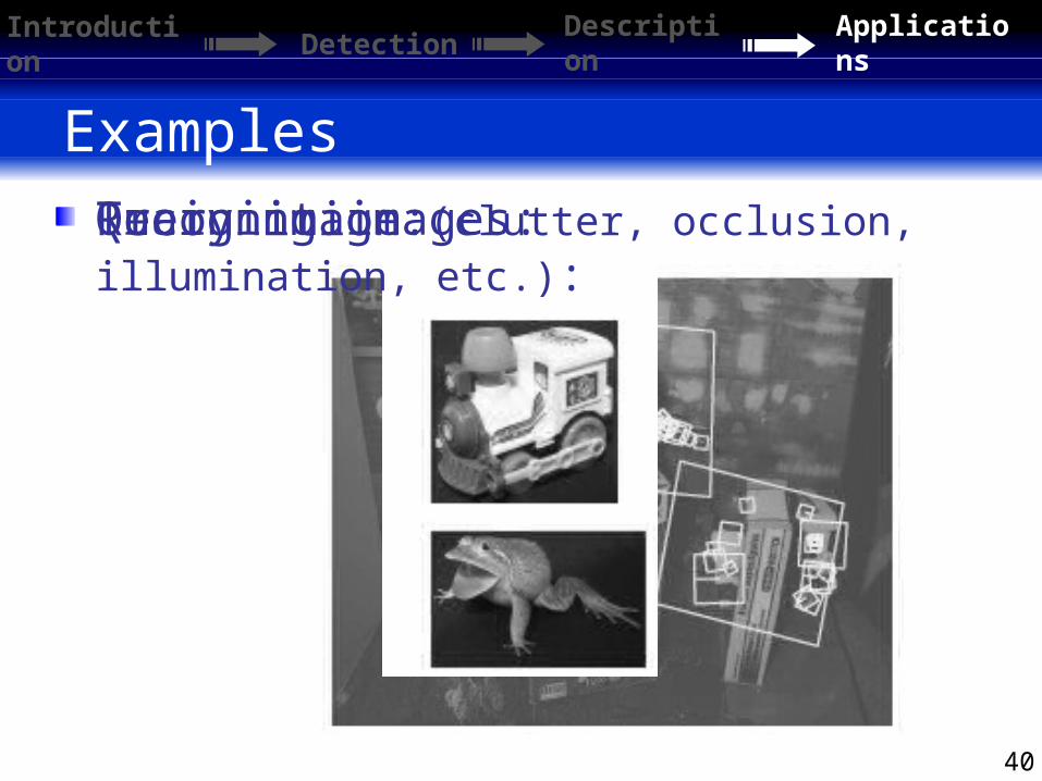
Examples
Introduction
Detection Description
Applications
Training images: Query image: Recognition (clutter, occlusion, illumination, etc.):
Page 41
41
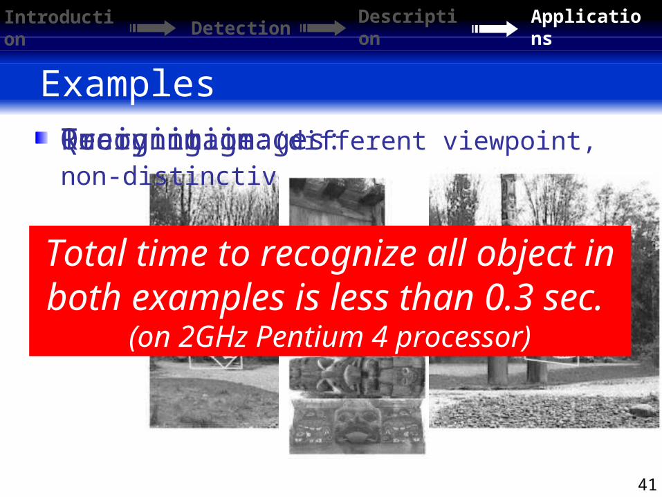
Examples
Introduction
Detection Description
Applications
Training images: Query image: Recognition (different viewpoint, non-distinctive):
Total time to recognize all object in both examples is less
than 0.3 sec. (on 2GHz Pentium 4 processor)
Page 42
42
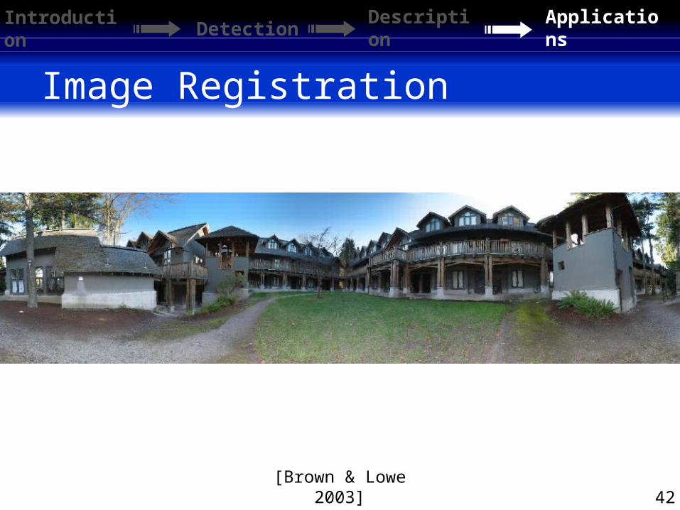
Image Registration
Introduction
Detection Description
Applications
[Brown & Lowe 2003]
Page 43
43
Examples
Introduction
Detection Description
Applications
Real time Object-Recognition:
Nose DEMO
Motion Tracking:
Recognition DEMO
Page 44
44
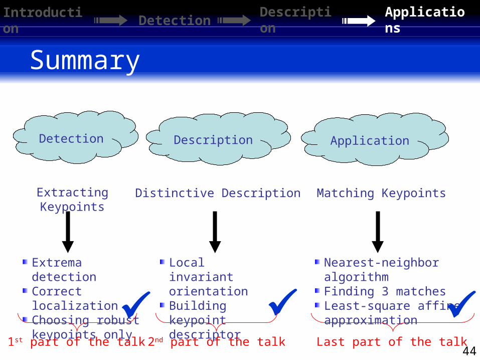
Nearest-neighbor algorithmFinding 3 matchesLeast-square affine approximation
Extrema detectionCorrect localizationChoosing robust keypoints only
Summary
Introduction
Detection Description
Applications
Distinctive Description Matching Keypoints
Local invariant orientationBuilding keypoint descriptor
Detection Description Application
1st part of the talk 2nd part of the talk Last part of the talk
Extracting Keypoints


![MSCOCO Keypoints Challenge 2017 - cocodataset.orgpresentations.cocodataset.org/COCO17-Keypoints-Megvii.pdfIs Hourglass good for COCO keypoint ResNet-FPN-like[1]network works better](https://static.documents.pub/doc/80x56/5f18bc4e82aff242ab772479/mscoco-keypoints-challenge-2017-is-hourglass-good-for-coco-keypoint-resnet-fpn-like1network.jpg)
