Olivier Cappe, Eric Moulines and Tobias Ryden

Inference in HiddenMarkov Models

May 22, 2007

Springer

Berlin Heidelberg NewYorkHongKong LondonMilan Paris Tokyo

Preface

Hidden Markov models—most often abbreviated to the acronym “HMMs”—are one of the most successful statistical modelling ideas that have came up inthe last forty years: the use of hidden (or unobservable) states makes the modelgeneric enough to handle a variety of complex real-world time series, while therelatively simple prior dependence structure (the “Markov” bit) still allowsfor the use of efficient computational procedures. Our goal with this book is topresent a reasonably complete picture of statistical inference for HMMs, fromthe simplest finite-valued models, which were already studied in the 1960’s,to recent topics like computational aspects of models with continuous statespace, asymptotics of maximum likelihood, Bayesian computation and modelselection, and all this illustrated with relevant running examples. We wantto stress at this point that by using the term hidden Markov model we donot limit ourselves to models with finite state space (for the hidden Markovchain), but also include models with continuous state space; such models areoften referred to as state-space models in the literature.

We build on the considerable developments that have taken place dur-ing the past ten years, both at the foundational level (asymptotics of maxi-mum likelihood estimates, order estimation, etc.) and at the computationallevel (variable dimension simulation, simulation-based optimization, etc.), topresent an up-to-date picture of the field that is self-contained from a theoret-ical point of view and self-sufficient from a methodological point of view. Wetherefore expect that the book will appeal to academic researchers in the fieldof HMMs, in particular PhD students working on related topics, by summingup the results obtained so far and presenting some new ideas. We hope that itwill similarly interest practitioners and researchers from other fields by lead-ing them through the computational steps required for making inference inHMMs and/or providing them with the relevant underlying statistical theory.

The book starts with an introductory chapter which explains, in simpleterms, what an HMM is, and it contains many examples of the use of HMMsin fields ranging from biology to telecommunications and finance. This chap-ter also describes various extension of HMMs, like models with autoregression

VI Preface

or hierarchical HMMs. Chapter 2 defines some basic concepts like transi-tion kernels and Markov chains. The remainder of the book is divided intothree parts: State Inference, Parameter Inference and Background and Com-plements; there are also three appendices.

Part I of the book covers inference for the unobserved state process. Westart in Chapter 3 by defining smoothing, filtering and predictive distributionsand describe the forward-backward decomposition and the corresponding re-cursions. We do this in a general framework with no assumption on finitenessof the hidden state space. The special cases of HMMs with finite state spaceand Gaussian linear state-space models are detailed in Chapter 5. Chapter 3also introduces the idea that the conditional distribution of the hidden Markovchain, given the observations, is Markov too, although non-homogeneous, forboth ordinary and time-reversed index orderings. As a result, two alternativealgorithms for smoothing are obtained. A major theme of Part I is simulation-based methods for state inference; Chapter 6 is a brief introduction to MonteCarlo simulation, and to Markov chain Monte Carlo and its applications toHMMs in particular, while Chapters 7 and 8 describe, starting from scratch,so-called sequential Monte Carlo (SMC) methods for approximating filteringand smoothing distributions in HMMs with continuous state space. Chapter 9is devoted to asymptotic analysis of SMC algorithms. More specialized top-ics of Part I include recursive computation of expectations of functions withrespect to smoothed distributions of the hidden chain (Section 4.1), SMC ap-proximations of such expectations (Section 8.3) and mixing properties of theconditional distribution of the hidden chain (Section 4.3). Variants of the ba-sic HMM structure like models with autoregression and hierarchical HMMsare considered in Sections 4.2, 6.3.2 and 8.2.

Part II of the book deals with inference for model parameters, mostlyfrom the maximum likelihood and Bayesian points of views. Chapter 10 de-scribes the expectation-maximization (EM) algorithm in detail, as well asits implementation for HMMs with finite state space and Gaussian linearstate-space models. This chapter also discusses likelihood maximization us-ing gradient-based optimization routines. HMMs with continuous state spacedo not generally admit exact implementation of EM, but require simulation-based methods. Chapter 11 covers various Monte Carlo algorithms like MonteCarlo EM, stochastic gradient algorithms and stochastic approximation EM.In addition to providing the algorithms and illustrative examples, it also con-tains an in-depth analysis of their convergence properties. Chapter 12 givesan overview of the framework for asymptotic analysis of the maximum like-lihood estimator, with some applications like asymptotics of likelihood-basedtests. Chapter 13 is about Bayesian inference for HMMs, with the focus beingon models with finite state space. It covers so-called reversible jump MCMCalgorithms for choosing between models of different dimensionality, and con-tains detailed examples illustrating these as well as simpler algorithms. It alsocontains a section on multiple imputation algorithms for global maximizationof the posterior density.

Preface VII

Part III of the book contains a chapter on discrete and general Markovchains, summarizing some of the most important concepts and results andapplying them to HMMs. The other chapter of this part focuses on orderestimation for HMMs with both finite state space and finite output alphabet;in particular it describes how concepts from information theory are useful forelaborating on this subject.

Various parts of the book require different amounts of, and also differentkinds of, prior knowledge from the reader. Generally we assume familiaritywith probability and statistical estimation at the levels of Feller (1971) andBickel and Doksum (1977), respectively. Some prior knowledge of Markovchains (discrete and/or general) is very helpful, although Part III does con-tain a primer on the topic; this chapter should however be considered morea brush-up than a comprehensive treatise of the subject. A reader with thatknowledge will be able to understand most parts of the book. Chapter 13 onBayesian estimation features a brief introduction to the subject in general but,again, some previous experience with Bayesian statistics will undoubtedly beof great help. The more theoretical parts of the book (Section 4.3, Chapter 9,Sections 11.2–11.3, Chapter 12, Sections 14.2–14.3 and Chapter 15) requireknowledge of probability theory at the measure-theoretic level for a full under-standing, even though most of the results as such can be understood withoutit.

There is no need to read the book in linear order, from cover to cover.Indeed, this is probably the wrong way to read it! Rather we encourage thereader to first go through the more algorithmic parts of the book, to get anoverall view of the subject, and then, if desired, later return to the theoreticalparts for a fuller understanding. Readers with particular topics in mind mayof course be even more selective. A reader interested in the EM algorithm,for instance, could start with Chapter 1, have a look at Chapter 2, and thenproceed to Chapter 3 before reading about the EM algorithm in Chapter 10.Similarly a reader interested in simulation-based techniques could go to Chap-ter 6 directly, perhaps after reading some of the introductory parts, or evendirectly to Section 6.3 if he/she is already familiar with MCMC methods.Each of the two chapters entitled “Advanced Topics in...” (Chapters 4 and 8)is really composed of three disconnected complements to Chapters 3 and 7,respectively. As such, the sections that compose Chapters 4 and 8 may beread independently of one another. Most chapters end with a section entitled“Complements” whose reading is not required for understanding other partsof the book—most often, this section mostly contains bibliographical notes—although in some chapters (9 and 11 in particular) it also features elementsneeded to prove the results stated in the main text.

Even in a book of this size, it is impossible to include all aspects of hiddenMarkov models. We have focused on the use of HMMs to model long, po-tentially stationary, time series; we call such models ergodic HMMs. In otherapplications, for instance speech recognition or protein alignment, HMMs areused to represent short variable-length sequences; such models are often called

VIII Preface

left-to-right HMMs and are hardly mentioned in this book. Having said thatwe stress that the computational tools for both classes of HMMs are virtuallythe same. There are also a number of generalizations of HMMs which we donot consider. In Markov random fields, as used in image processing applica-tions, the Markov chain is replaced by a graph of dependency which may berepresented as a two-dimensional regular lattice. The numerical techniquesthat can be used for inference in hidden Markov random fields are similar tosome of the methods studied in this book but the statistical side is very differ-ent. Bayesian networks are even more general since the dependency structureis allowed to take any form represented by a (directed or undirected) graph.We do not consider Bayesian networks in their generality although some ofthe concepts developed in the Bayesian networks literature (the graph repre-sentation, the sum-product algorithm) are used. Continuous-time HMMs mayalso be seen as a further generalization of the models considered in this book.Some of these “continuous-time HMMs”, and in particular partially observeddiffusion models used in mathematical finance, have recently received consid-erable attention. We however decided this topic to be outside the range ofthe book; furthermore, the stochastic calculus tools needed for studying thesecontinuous-time models are not appropriate for our purpose.

We acknowledge the help of Stephane Boucheron, Randal Douc, GersendeFort, Elisabeth Gassiat, Christian P. Robert, and Philippe Soulier, who par-ticipated in the writing of the text and contributed the two chapters thatcompose Part III (see next page for details of the contributions). We are alsoindebted to them for suggesting various forms of improvement in the nota-tions, layout, etc., as well as helping us track typos and errors. We thankFrancois Le Gland and Catherine Matias for participating in the early stagesof this book project. We are grateful to Christophe Andrieu, Søren Asmussen,Arnaud Doucet, Hans Kunsch, Steve Levinson, Ya’acov Ritov and Mike Tit-terington, who provided various helpful inputs and comments. Finally, wethank John Kimmel of Springer for his support and enduring patience.

Paris, France Olivier Cappe& Lund, Sweden Eric MoulinesMarch 2005 Tobias Ryden

Contributors

We are grateful to

Randal DoucEcole PolytechniqueChristian P. RobertCREST INSEE & Universite Paris-Dauphine

for their contributions to Chapters 9 (Randal) and 6, 7, and 13 (Christian) aswell as for their help in proofreading these and other parts of the book

Chapter 14 was written by

Gersende FortCNRS & LMC-IMAGPhilippe SoulierUniversite Paris-Nanterre

with Eric Moulines

Chapter 15 was written by

Stephane BoucheronUniversite Paris VII-Denis DiderotElisabeth GassiatUniversite d’Orsay, Paris-Sud

Contents

Preface . . . . . . . . . . . . . . . . . . . . . . . . . . . . . . . . . . . . . . . . . . . . . . . . . . . . . . . . V

Contributors . . . . . . . . . . . . . . . . . . . . . . . . . . . . . . . . . . . . . . . . . . . . . . . . . . . IX

1 Introduction . . . . . . . . . . . . . . . . . . . . . . . . . . . . . . . . . . . . . . . . . . . . . . . 11.1 What Is a Hidden Markov Model? . . . . . . . . . . . . . . . . . . . . . . . . . 11.2 Beyond Hidden Markov Models . . . . . . . . . . . . . . . . . . . . . . . . . . . 41.3 Examples . . . . . . . . . . . . . . . . . . . . . . . . . . . . . . . . . . . . . . . . . . . . . . . 6

1.3.1 Finite Hidden Markov Models . . . . . . . . . . . . . . . . . . . . . . . 61.3.2 Normal Hidden Markov Models . . . . . . . . . . . . . . . . . . . . . 131.3.3 Gaussian Linear State-Space Models . . . . . . . . . . . . . . . . . 151.3.4 Conditionally Gaussian Linear State-Space Models . . . . 171.3.5 General (Continuous) State-Space HMMs . . . . . . . . . . . . 231.3.6 Switching Processes with Markov Regime . . . . . . . . . . . . . 29

1.4 Left-to-Right and Ergodic Hidden Markov Models . . . . . . . . . . . 33

2 Main Definitions and Notations . . . . . . . . . . . . . . . . . . . . . . . . . . . . 352.1 Markov Chains . . . . . . . . . . . . . . . . . . . . . . . . . . . . . . . . . . . . . . . . . . 35

2.1.1 Transition Kernels . . . . . . . . . . . . . . . . . . . . . . . . . . . . . . . . . 352.1.2 Homogeneous Markov Chains . . . . . . . . . . . . . . . . . . . . . . . 372.1.3 Non-homogeneous Markov Chains . . . . . . . . . . . . . . . . . . . 40

2.2 Hidden Markov Models . . . . . . . . . . . . . . . . . . . . . . . . . . . . . . . . . . . 422.2.1 Definitions and Notations . . . . . . . . . . . . . . . . . . . . . . . . . . 422.2.2 Conditional Independence in Hidden Markov Models . . . 442.2.3 Hierarchical Hidden Markov Models . . . . . . . . . . . . . . . . . 46

Part I State Inference

XII Contents

3 Filtering and Smoothing Recursions . . . . . . . . . . . . . . . . . . . . . . . 513.1 Basic Notations and Definitions . . . . . . . . . . . . . . . . . . . . . . . . . . . 52

3.1.1 Likelihood . . . . . . . . . . . . . . . . . . . . . . . . . . . . . . . . . . . . . . . . 533.1.2 Smoothing . . . . . . . . . . . . . . . . . . . . . . . . . . . . . . . . . . . . . . . . 543.1.3 The Forward-Backward Decomposition . . . . . . . . . . . . . . . 563.1.4 Implicit Conditioning (Please Read This Section!) . . . . . 58

3.2 Forward-Backward . . . . . . . . . . . . . . . . . . . . . . . . . . . . . . . . . . . . . . . 593.2.1 The Forward-Backward Recursions . . . . . . . . . . . . . . . . . . 593.2.2 Filtering and Normalized Recursion . . . . . . . . . . . . . . . . . . 61

3.3 Markovian Decompositions . . . . . . . . . . . . . . . . . . . . . . . . . . . . . . . 663.3.1 Forward Decomposition . . . . . . . . . . . . . . . . . . . . . . . . . . . . 663.3.2 Backward Decomposition . . . . . . . . . . . . . . . . . . . . . . . . . . . 70

3.4 Complements . . . . . . . . . . . . . . . . . . . . . . . . . . . . . . . . . . . . . . . . . . . 74

4 Advanced Topics in Smoothing . . . . . . . . . . . . . . . . . . . . . . . . . . . . 774.1 Recursive Computation of Smoothed Functionals . . . . . . . . . . . . 77

4.1.1 Fixed Point Smoothing . . . . . . . . . . . . . . . . . . . . . . . . . . . . . 784.1.2 Recursive Smoothers for General Functionals . . . . . . . . . 794.1.3 Comparison with Forward-Backward Smoothing . . . . . . . 82

4.2 Filtering and Smoothing in More General Models . . . . . . . . . . . . 854.2.1 Smoothing in Markov-switching Models . . . . . . . . . . . . . . 864.2.2 Smoothing in Partially Observed Markov Chains . . . . . . 864.2.3 Marginal Smoothing in Hierarchical HMMs . . . . . . . . . . . 87

4.3 Forgetting of the Initial Condition . . . . . . . . . . . . . . . . . . . . . . . . . 894.3.1 Total Variation. . . . . . . . . . . . . . . . . . . . . . . . . . . . . . . . . . . . 904.3.2 Lipshitz Contraction for Transition Kernels . . . . . . . . . . . 954.3.3 The Doeblin Condition and Uniform Ergodicity . . . . . . . 974.3.4 Forgetting Properties . . . . . . . . . . . . . . . . . . . . . . . . . . . . . . 1004.3.5 Uniform Forgetting Under Strong Mixing Conditions . . . 1054.3.6 Forgetting Under Alternative Conditions . . . . . . . . . . . . . 110

5 Applications of Smoothing . . . . . . . . . . . . . . . . . . . . . . . . . . . . . . . . . 1215.1 Models with Finite State Space . . . . . . . . . . . . . . . . . . . . . . . . . . . 121

5.1.1 Smoothing . . . . . . . . . . . . . . . . . . . . . . . . . . . . . . . . . . . . . . . . 1225.1.2 Maximum a Posteriori Sequence Estimation . . . . . . . . . . 125

5.2 Gaussian Linear State-Space Models . . . . . . . . . . . . . . . . . . . . . . . 1275.2.1 Filtering and Backward Markovian Smoothing . . . . . . . . 1275.2.2 Linear Prediction Interpretation . . . . . . . . . . . . . . . . . . . . . 1315.2.3 The Prediction and Filtering Recursions Revisited . . . . . 1375.2.4 Disturbance Smoothing . . . . . . . . . . . . . . . . . . . . . . . . . . . . 1435.2.5 The Backward Recursion and the Two-Filter Formula . . 1475.2.6 Application to Marginal Filtering and Smoothing in

CGLSSMs . . . . . . . . . . . . . . . . . . . . . . . . . . . . . . . . . . . . . . . . 154

Contents XIII

6 Monte Carlo Methods . . . . . . . . . . . . . . . . . . . . . . . . . . . . . . . . . . . . . 1616.1 Basic Monte Carlo Methods . . . . . . . . . . . . . . . . . . . . . . . . . . . . . . 161

6.1.1 Monte Carlo Integration . . . . . . . . . . . . . . . . . . . . . . . . . . . . 1616.1.2 Monte Carlo Simulation for HMM State Inference . . . . . 163

6.2 A Markov Chain Monte Carlo Primer . . . . . . . . . . . . . . . . . . . . . . 1656.2.1 The Accept-Reject Algorithm . . . . . . . . . . . . . . . . . . . . . . . 1666.2.2 Markov Chain Monte Carlo . . . . . . . . . . . . . . . . . . . . . . . . . 1696.2.3 Metropolis-Hastings . . . . . . . . . . . . . . . . . . . . . . . . . . . . . . . 1716.2.4 Hybrid Algorithms . . . . . . . . . . . . . . . . . . . . . . . . . . . . . . . . 1786.2.5 Gibbs Sampling . . . . . . . . . . . . . . . . . . . . . . . . . . . . . . . . . . . 1806.2.6 Stopping an MCMC Algorithm. . . . . . . . . . . . . . . . . . . . . . 185

6.3 Applications to Hidden Markov Models . . . . . . . . . . . . . . . . . . . . 1866.3.1 Generic Sampling Strategies . . . . . . . . . . . . . . . . . . . . . . . . 1866.3.2 Gibbs Sampling in CGLSSMs . . . . . . . . . . . . . . . . . . . . . . . 194

7 Sequential Monte Carlo Methods . . . . . . . . . . . . . . . . . . . . . . . . . . 2097.1 Importance Sampling and Resampling . . . . . . . . . . . . . . . . . . . . . . 210

7.1.1 Importance Sampling . . . . . . . . . . . . . . . . . . . . . . . . . . . . . . 2107.1.2 Sampling Importance Resampling . . . . . . . . . . . . . . . . . . . 211

7.2 Sequential Importance Sampling . . . . . . . . . . . . . . . . . . . . . . . . . . . 2147.2.1 Sequential Implementation for HMMs . . . . . . . . . . . . . . . . 2147.2.2 Choice of the Instrumental Kernel . . . . . . . . . . . . . . . . . . . 218

7.3 Sequential Importance Sampling with Resampling . . . . . . . . . . . 2317.3.1 Weight Degeneracy . . . . . . . . . . . . . . . . . . . . . . . . . . . . . . . . 2317.3.2 Resampling . . . . . . . . . . . . . . . . . . . . . . . . . . . . . . . . . . . . . . . 236

7.4 Complements . . . . . . . . . . . . . . . . . . . . . . . . . . . . . . . . . . . . . . . . . . . 2427.4.1 Implementation of Multinomial Resampling . . . . . . . . . . . 2427.4.2 Alternatives to Multinomial Resampling . . . . . . . . . . . . . . 244

8 Advanced Topics in Sequential Monte Carlo . . . . . . . . . . . . . . . 2518.1 Alternatives to SISR . . . . . . . . . . . . . . . . . . . . . . . . . . . . . . . . . . . . . 251

8.1.1 I.I.D. Sampling . . . . . . . . . . . . . . . . . . . . . . . . . . . . . . . . . . . 2538.1.2 Two-Stage Sampling . . . . . . . . . . . . . . . . . . . . . . . . . . . . . . . 2568.1.3 Interpretation with Auxiliary Variables . . . . . . . . . . . . . . . 2608.1.4 Auxiliary Accept-Reject Sampling . . . . . . . . . . . . . . . . . . . 2618.1.5 Markov Chain Monte Carlo Auxiliary Sampling . . . . . . . 263

8.2 Sequential Monte Carlo in Hierarchical HMMs . . . . . . . . . . . . . . 2648.2.1 Sequential Importance Sampling and Global Sampling . 2658.2.2 Optimal Sampling . . . . . . . . . . . . . . . . . . . . . . . . . . . . . . . . . 2678.2.3 Application to CGLSSMs. . . . . . . . . . . . . . . . . . . . . . . . . . . 273

8.3 Particle Approximation of Smoothing Functionals . . . . . . . . . . . 278

XIV Contents

9 Analysis of Sequential Monte Carlo Methods . . . . . . . . . . . . . . 2879.1 Importance Sampling . . . . . . . . . . . . . . . . . . . . . . . . . . . . . . . . . . . . 287

9.1.1 Unnormalized Importance Sampling . . . . . . . . . . . . . . . . . 2879.1.2 Deviation Inequalities . . . . . . . . . . . . . . . . . . . . . . . . . . . . . . 2919.1.3 Self-normalized Importance Sampling Estimator . . . . . . . 293

9.2 Sampling Importance Resampling . . . . . . . . . . . . . . . . . . . . . . . . . 2959.2.1 The Algorithm . . . . . . . . . . . . . . . . . . . . . . . . . . . . . . . . . . . . 2959.2.2 Definitions and Notations . . . . . . . . . . . . . . . . . . . . . . . . . . 2979.2.3 Weighting and Resampling . . . . . . . . . . . . . . . . . . . . . . . . . 3009.2.4 Application to the Single-Stage SIR Algorithm . . . . . . . . 307

9.3 Single-Step Analysis of SMC Methods . . . . . . . . . . . . . . . . . . . . . . 3119.3.1 Mutation Step . . . . . . . . . . . . . . . . . . . . . . . . . . . . . . . . . . . . 3119.3.2 Description of Algorithms . . . . . . . . . . . . . . . . . . . . . . . . . . 3159.3.3 Analysis of the Mutation/Selection Algorithm . . . . . . . . . 3199.3.4 Analysis of the Selection/Mutation Algorithm . . . . . . . . . 320

9.4 Sequential Monte Carlo Methods . . . . . . . . . . . . . . . . . . . . . . . . . . 3219.4.1 SISR . . . . . . . . . . . . . . . . . . . . . . . . . . . . . . . . . . . . . . . . . . . . 3219.4.2 I.I.D. Sampling . . . . . . . . . . . . . . . . . . . . . . . . . . . . . . . . . . . 324

9.5 Complements . . . . . . . . . . . . . . . . . . . . . . . . . . . . . . . . . . . . . . . . . . . 3339.5.1 Weak Limits Theorems for Triangular Array . . . . . . . . . . 3339.5.2 Bibliographic Notes . . . . . . . . . . . . . . . . . . . . . . . . . . . . . . . . 342

Part II Parameter Inference

10 Maximum Likelihood Inference, Part I:Optimization Through Exact Smoothing . . . . . . . . . . . . . . . . . . . 34510.1 Likelihood Optimization in Incomplete Data Models . . . . . . . . . 345

10.1.1 Problem Statement and Notations . . . . . . . . . . . . . . . . . . . 34610.1.2 The Expectation-Maximization Algorithm . . . . . . . . . . . . 34710.1.3 Gradient-based Methods . . . . . . . . . . . . . . . . . . . . . . . . . . . 35110.1.4 Pros and Cons of Gradient-based Methods . . . . . . . . . . . . 356

10.2 Application to HMMs . . . . . . . . . . . . . . . . . . . . . . . . . . . . . . . . . . . . 35710.2.1 Hidden Markov Models as Missing Data Models . . . . . . . 35710.2.2 EM in HMMs . . . . . . . . . . . . . . . . . . . . . . . . . . . . . . . . . . . . . 35810.2.3 Computing Derivatives . . . . . . . . . . . . . . . . . . . . . . . . . . . . . 36010.2.4 Connection with the Sensitivity Equation Approach . . . 362

10.3 The Example of Normal Hidden Markov Models . . . . . . . . . . . . . 36510.3.1 EM Parameter Update Formulas . . . . . . . . . . . . . . . . . . . . 36510.3.2 Estimation of the Initial Distribution . . . . . . . . . . . . . . . . 36810.3.3 Recursive Implementation of E-Step . . . . . . . . . . . . . . . . . 36810.3.4 Computation of the Score and Observed Information . . . 372

10.4 The Example of Gaussian Linear State-Space Models . . . . . . . . 38210.4.1 The Intermediate Quantity of EM . . . . . . . . . . . . . . . . . . . 38310.4.2 Recursive Implementation . . . . . . . . . . . . . . . . . . . . . . . . . . 385

Contents XV

10.5 Complements . . . . . . . . . . . . . . . . . . . . . . . . . . . . . . . . . . . . . . . . . . . 38710.5.1 Global Convergence of the EM Algorithm . . . . . . . . . . . . 38710.5.2 Rate of Convergence of EM . . . . . . . . . . . . . . . . . . . . . . . . . 39010.5.3 Generalized EM Algorithms . . . . . . . . . . . . . . . . . . . . . . . . 39110.5.4 Bibliographic Notes . . . . . . . . . . . . . . . . . . . . . . . . . . . . . . . . 392

11 Maximum Likelihood Inference, Part II:Monte Carlo Optimization . . . . . . . . . . . . . . . . . . . . . . . . . . . . . . . . . 39511.1 Methods and Algorithms . . . . . . . . . . . . . . . . . . . . . . . . . . . . . . . . . 396

11.1.1 Monte Carlo EM . . . . . . . . . . . . . . . . . . . . . . . . . . . . . . . . . . 39611.1.2 Simulation Schedules . . . . . . . . . . . . . . . . . . . . . . . . . . . . . . 40111.1.3 Gradient-based Algorithms . . . . . . . . . . . . . . . . . . . . . . . . . 40611.1.4 Interlude: Stochastic Approximation and the

Robbins-Monro Approach . . . . . . . . . . . . . . . . . . . . . . . . . . 40911.1.5 Stochastic Gradient Algorithms . . . . . . . . . . . . . . . . . . . . . 41011.1.6 Stochastic Approximation EM . . . . . . . . . . . . . . . . . . . . . . 41211.1.7 Stochastic EM . . . . . . . . . . . . . . . . . . . . . . . . . . . . . . . . . . . . 414

11.2 Analysis of the MCEM Algorithm . . . . . . . . . . . . . . . . . . . . . . . . . 41711.2.1 Convergence of Perturbed Dynamical Systems . . . . . . . . 41811.2.2 Convergence of the MCEM Algorithm . . . . . . . . . . . . . . . 42011.2.3 Rate of Convergence of MCEM . . . . . . . . . . . . . . . . . . . . . 424

11.3 Analysis of Stochastic Approximation Algorithms . . . . . . . . . . . . 42711.3.1 Basic Results for Stochastic Approximation

Algorithms . . . . . . . . . . . . . . . . . . . . . . . . . . . . . . . . . . . . . . . 42711.3.2 Convergence of the Stochastic Gradient Algorithm . . . . . 42811.3.3 Rate of Convergence of the Stochastic Gradient

Algorithm . . . . . . . . . . . . . . . . . . . . . . . . . . . . . . . . . . . . . . . . 43011.3.4 Convergence of the SAEM Algorithm . . . . . . . . . . . . . . . . 431

11.4 Complements . . . . . . . . . . . . . . . . . . . . . . . . . . . . . . . . . . . . . . . . . . . 433

12 Statistical Properties of the Maximum LikelihoodEstimator . . . . . . . . . . . . . . . . . . . . . . . . . . . . . . . . . . . . . . . . . . . . . . . . . . 43912.1 A Primer on MLE Asymptotics . . . . . . . . . . . . . . . . . . . . . . . . . . . 44012.2 Stationary Approximations . . . . . . . . . . . . . . . . . . . . . . . . . . . . . . . 44112.3 Consistency . . . . . . . . . . . . . . . . . . . . . . . . . . . . . . . . . . . . . . . . . . . . . 444

12.3.1 Construction of the Stationary ConditionalLog-likelihood . . . . . . . . . . . . . . . . . . . . . . . . . . . . . . . . . . . . . 444

12.3.2 The Contrast Function and Its Properties . . . . . . . . . . . . 44612.4 Identifiability . . . . . . . . . . . . . . . . . . . . . . . . . . . . . . . . . . . . . . . . . . . 448

12.4.1 Equivalence of Parameters . . . . . . . . . . . . . . . . . . . . . . . . . . 44912.4.2 Identifiability of Mixture Densities . . . . . . . . . . . . . . . . . . . 45212.4.3 Application of Mixture Identifiability to Hidden

Markov Models . . . . . . . . . . . . . . . . . . . . . . . . . . . . . . . . . . . 45312.5 Asymptotic Normality of the Score and Convergence of the

Observed Information . . . . . . . . . . . . . . . . . . . . . . . . . . . . . . . . . . . . 455

XVI Contents

12.5.1 The Score Function and Invoking the Fisher Identity . . . 45512.5.2 Construction of the Stationary Conditional Score . . . . . . 45712.5.3 Weak Convergence of the Normalized Score . . . . . . . . . . . 46212.5.4 Convergence of the Normalized Observed Information . . 46312.5.5 Asymptotics of the Maximum Likelihood Estimator . . . . 463

12.6 Applications to Likelihood-based Tests . . . . . . . . . . . . . . . . . . . . . 46412.7 Complements . . . . . . . . . . . . . . . . . . . . . . . . . . . . . . . . . . . . . . . . . . . 466

13 Fully Bayesian Approaches . . . . . . . . . . . . . . . . . . . . . . . . . . . . . . . . 46913.1 Parameter Estimation . . . . . . . . . . . . . . . . . . . . . . . . . . . . . . . . . . . . 469

13.1.1 Bayesian Inference . . . . . . . . . . . . . . . . . . . . . . . . . . . . . . . . . 46913.1.2 Prior Distributions for HMMs . . . . . . . . . . . . . . . . . . . . . . . 47313.1.3 Non-identifiability and Label Switching . . . . . . . . . . . . . . 47613.1.4 MCMC Methods for Bayesian Inference . . . . . . . . . . . . . . 479

13.2 Reversible Jump Methods . . . . . . . . . . . . . . . . . . . . . . . . . . . . . . . . 48613.2.1 Variable Dimension Models . . . . . . . . . . . . . . . . . . . . . . . . . 48613.2.2 Green’s Reversible Jump Algorithm. . . . . . . . . . . . . . . . . . 48813.2.3 Alternative Sampler Designs . . . . . . . . . . . . . . . . . . . . . . . . 49613.2.4 Alternatives to Reversible Jump MCMC . . . . . . . . . . . . . 498

13.3 Multiple Imputations Methods and Maximum a Posteriori . . . 49913.3.1 Simulated Annealing . . . . . . . . . . . . . . . . . . . . . . . . . . . . . . . 50013.3.2 The SAME Algorithm . . . . . . . . . . . . . . . . . . . . . . . . . . . . . 500

Part III Background and Complements

14 Elements of Markov Chain Theory . . . . . . . . . . . . . . . . . . . . . . . . 51114.1 Chains on Countable State Spaces . . . . . . . . . . . . . . . . . . . . . . . . . 511

14.1.1 Irreducibility . . . . . . . . . . . . . . . . . . . . . . . . . . . . . . . . . . . . . 51114.1.2 Recurrence and Transience . . . . . . . . . . . . . . . . . . . . . . . . . 51214.1.3 Invariant Measures and Stationarity . . . . . . . . . . . . . . . . . 51514.1.4 Ergodicity . . . . . . . . . . . . . . . . . . . . . . . . . . . . . . . . . . . . . . . . 517

14.2 Chains on General State Spaces . . . . . . . . . . . . . . . . . . . . . . . . . . . 51814.2.1 Irreducibility . . . . . . . . . . . . . . . . . . . . . . . . . . . . . . . . . . . . . 51914.2.2 Recurrence and Transience . . . . . . . . . . . . . . . . . . . . . . . . . 52114.2.3 Invariant Measures and Stationarity . . . . . . . . . . . . . . . . . 53214.2.4 Ergodicity . . . . . . . . . . . . . . . . . . . . . . . . . . . . . . . . . . . . . . . . 53914.2.5 Geometric Ergodicity and Foster-Lyapunov Conditions . 54614.2.6 Limit Theorems . . . . . . . . . . . . . . . . . . . . . . . . . . . . . . . . . . . 550

14.3 Applications to Hidden Markov Models . . . . . . . . . . . . . . . . . . . . 55414.3.1 Phi-irreducibility . . . . . . . . . . . . . . . . . . . . . . . . . . . . . . . . . . 55414.3.2 Atoms and Small Sets . . . . . . . . . . . . . . . . . . . . . . . . . . . . . . 55614.3.3 Recurrence and Positive Recurrence . . . . . . . . . . . . . . . . . 558

Contents XVII

15 An Information-Theoretic Perspective on OrderEstimation . . . . . . . . . . . . . . . . . . . . . . . . . . . . . . . . . . . . . . . . . . . . . . . . . 56315.1 Model Order Identification: What Is It About? . . . . . . . . . . . . . . 56415.2 Order Estimation in Perspective . . . . . . . . . . . . . . . . . . . . . . . . . . . 56515.3 Order Estimation and Composite Hypothesis Testing . . . . . . . . 56715.4 Code-based Identification . . . . . . . . . . . . . . . . . . . . . . . . . . . . . . . . . 569

15.4.1 Definitions . . . . . . . . . . . . . . . . . . . . . . . . . . . . . . . . . . . . . . . 56915.4.2 Information Divergence Rates . . . . . . . . . . . . . . . . . . . . . . . 572

15.5 MDL Order Estimators in Bayesian Settings . . . . . . . . . . . . . . . . 57415.6 Strongly Consistent Penalized Maximum Likelihood

Estimators for HMM Order Estimation . . . . . . . . . . . . . . . . . . . . . 57515.7 Efficiency Issues . . . . . . . . . . . . . . . . . . . . . . . . . . . . . . . . . . . . . . . . . 578

15.7.1 Variations on Stein’s Lemma . . . . . . . . . . . . . . . . . . . . . . . 57915.7.2 Achieving Optimal Error Exponents . . . . . . . . . . . . . . . . . 582

15.8 Consistency of the BIC Estimator in the Markov OrderEstimation Problem . . . . . . . . . . . . . . . . . . . . . . . . . . . . . . . . . . . . . 58515.8.1 Some Martingale Tools . . . . . . . . . . . . . . . . . . . . . . . . . . . . . 58715.8.2 The Martingale Approach . . . . . . . . . . . . . . . . . . . . . . . . . . 58915.8.3 The Union Bound Meets Martingale Inequalities . . . . . . 590

15.9 Complements . . . . . . . . . . . . . . . . . . . . . . . . . . . . . . . . . . . . . . . . . . . 598

Part IV Appendices

A Conditioning . . . . . . . . . . . . . . . . . . . . . . . . . . . . . . . . . . . . . . . . . . . . . . 603A.1 Probability and Topology Terminology and Notation . . . . . . . . . 603A.2 Conditional Expectation . . . . . . . . . . . . . . . . . . . . . . . . . . . . . . . . . . 604A.3 Conditional Distribution . . . . . . . . . . . . . . . . . . . . . . . . . . . . . . . . . 609A.4 Conditional Independence . . . . . . . . . . . . . . . . . . . . . . . . . . . . . . . . 612

B Linear Prediction . . . . . . . . . . . . . . . . . . . . . . . . . . . . . . . . . . . . . . . . . . 615B.1 Hilbert Spaces . . . . . . . . . . . . . . . . . . . . . . . . . . . . . . . . . . . . . . . . . . 615B.2 The Projection Theorem . . . . . . . . . . . . . . . . . . . . . . . . . . . . . . . . . 617

C Notations . . . . . . . . . . . . . . . . . . . . . . . . . . . . . . . . . . . . . . . . . . . . . . . . . . 619C.1 Mathematical . . . . . . . . . . . . . . . . . . . . . . . . . . . . . . . . . . . . . . . . . . . 619C.2 Probability . . . . . . . . . . . . . . . . . . . . . . . . . . . . . . . . . . . . . . . . . . . . . 620C.3 Hidden Markov Models . . . . . . . . . . . . . . . . . . . . . . . . . . . . . . . . . . . 620C.4 Sequential Monte Carlo . . . . . . . . . . . . . . . . . . . . . . . . . . . . . . . . . . 622

References . . . . . . . . . . . . . . . . . . . . . . . . . . . . . . . . . . . . . . . . . . . . . . . . . . . . . 623

Index . . . . . . . . . . . . . . . . . . . . . . . . . . . . . . . . . . . . . . . . . . . . . . . . . . . . . . . . . . 643

1

Introduction

1.1 What Is a Hidden Markov Model?

A hidden Markov model (abbreviated HMM) is, loosely speaking, a Markovchain observed in noise. Indeed, the model comprises a Markov chain, whichwe will denote by Xkk≥0, where k is an integer index. This Markov chainis often assumed to take values in a finite set, but we will not make thisrestriction in general, thus allowing for a quite arbitrary state space. Now,the Markov chain is hidden, that is, it is not observable. What is available tothe observer is another stochastic process Ykk≥0, linked to the Markov chainin that Xk governs the distribution of the corresponding Yk. For instance, Ykmay have a normal distribution, the mean and variance of which is determinedby Xk, or Yk may have a Poisson distribution whose mean is determined byXk. The underlying Markov chain Xk is sometimes called the regime, orstate. All statistical inference, even on the Markov chain itself, has to bedone in terms of Yk only, as Xk is not observed. There is also a furtherassumption on the relation between the Markov chain and the observableprocess, saying that Xk must be the only variable of the Markov chain thataffects the distribution of Yk. This is expressed more precisely in the followingformal definition.

A hidden Markov model is a bivariate discrete time process Xk, Ykk≥0,where Xk is a Markov chain and, conditional on Xk, Yk is a sequenceof independent random variables such that the conditional distribution of Ykonly depends on Xk. We will denote the state space of the Markov chain Xkby X and the set in which Yk takes its values by Y.

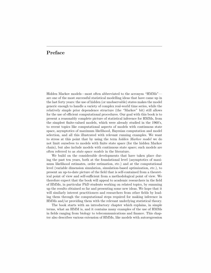
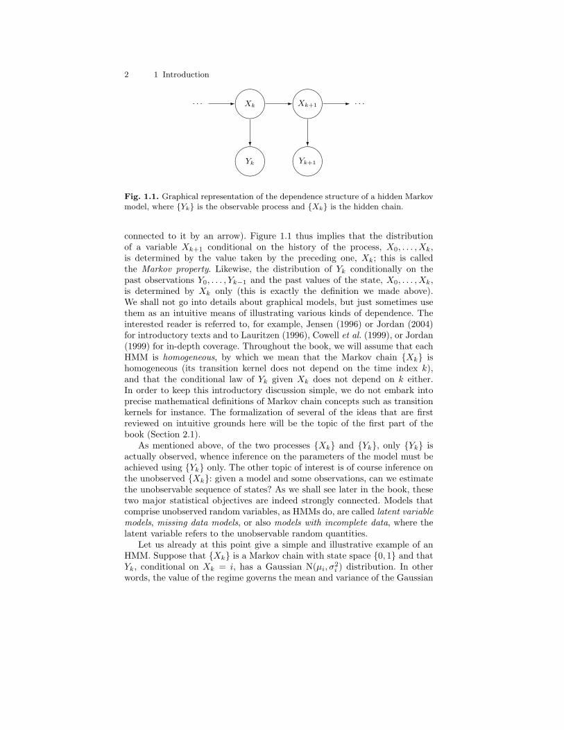
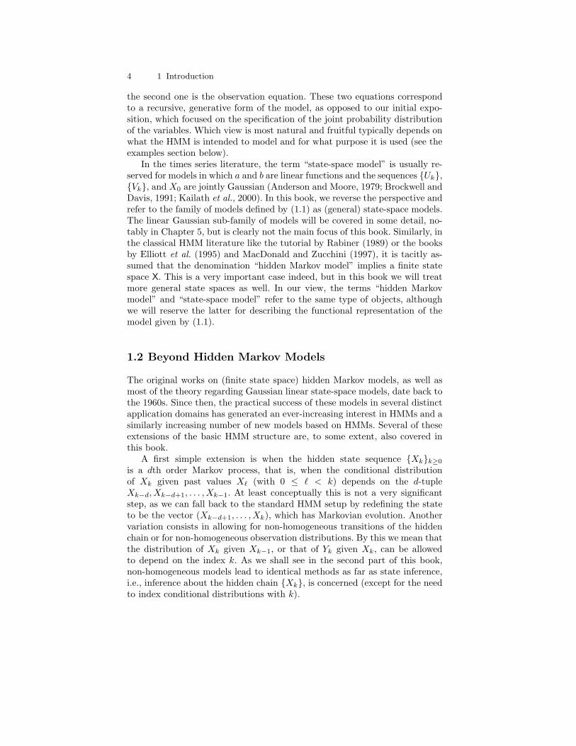
The dependence structure of an HMM can be represented by a graphicalmodel as in Figure 1.1. Representations of this sort use a directed graphwithout loops to describe dependence structures among random variables. Thenodes (circles) in the graph correspond to the random variables, and the edges(arrows) represent the structure of the joint probability distribution, with theinterpretation that the latter may be factored as a product of the conditionaldistributions of each node given its “parent” nodes (those that are directly

2 1 Introduction

· · · -

-

- · · ·

?

?

Xk Xk+1

Yk Yk+1

Fig. 1.1. Graphical representation of the dependence structure of a hidden Markovmodel, where Yk is the observable process and Xk is the hidden chain.

connected to it by an arrow). Figure 1.1 thus implies that the distributionof a variable Xk+1 conditional on the history of the process, X0, . . . , Xk,is determined by the value taken by the preceding one, Xk; this is calledthe Markov property. Likewise, the distribution of Yk conditionally on thepast observations Y0, . . . , Yk−1 and the past values of the state, X0, . . . , Xk,is determined by Xk only (this is exactly the definition we made above).We shall not go into details about graphical models, but just sometimes usethem as an intuitive means of illustrating various kinds of dependence. Theinterested reader is referred to, for example, Jensen (1996) or Jordan (2004)for introductory texts and to Lauritzen (1996), Cowell et al. (1999), or Jordan(1999) for in-depth coverage. Throughout the book, we will assume that eachHMM is homogeneous, by which we mean that the Markov chain Xk ishomogeneous (its transition kernel does not depend on the time index k),and that the conditional law of Yk given Xk does not depend on k either.In order to keep this introductory discussion simple, we do not embark intoprecise mathematical definitions of Markov chain concepts such as transitionkernels for instance. The formalization of several of the ideas that are firstreviewed on intuitive grounds here will be the topic of the first part of thebook (Section 2.1).

As mentioned above, of the two processes Xk and Yk, only Yk isactually observed, whence inference on the parameters of the model must beachieved using Yk only. The other topic of interest is of course inference onthe unobserved Xk: given a model and some observations, can we estimatethe unobservable sequence of states? As we shall see later in the book, thesetwo major statistical objectives are indeed strongly connected. Models thatcomprise unobserved random variables, as HMMs do, are called latent variablemodels, missing data models, or also models with incomplete data, where thelatent variable refers to the unobservable random quantities.

Let us already at this point give a simple and illustrative example of anHMM. Suppose that Xk is a Markov chain with state space 0, 1 and thatYk, conditional on Xk = i, has a Gaussian N(µi, σ2

i ) distribution. In otherwords, the value of the regime governs the mean and variance of the Gaussian

1.1 What Is a Hidden Markov Model? 3

distribution from which we then draw the output. This model illustrates acommon feature of HMMs considered in this book, namely that the condi-tional distributions of Yk given Xk all belong to a single parametric family,with parameters indexed by Xk. In this case, it is the Gaussian family ofdistributions, but one may of course also consider the Gamma family, thePoisson family, etc. A meaningful observation, in the current example, is thatthe marginal distribution of Yk is that of a mixture of two Gaussian dis-tributions. Hence we may also view HMMs as an extension of independentmixture models, including some degree of dependence between observations.

Indeed, even though the Y -variables are conditionally independent givenXk, Yk is not an independent sequence because of the dependence inXk. In fact, Yk is not a Markov chain either: the joint process Xk, Yk isof course a Markov chain, but the observable process Yk does not have theloss of memory property of Markov chains, in the sense that the conditionaldistribution of Yk given Y0, . . . , Yk−1 generally depends on all the condition-ing variables. As we shall see in Chapter 2, however, the dependence in thesequence Yk (defined in a suitable sense) is not stronger than that in Xk.This is a general observation that is valid not only for the current example.

Another view is to consider HMMs as an extension of Markov chains, inwhich the observation Yk of the state Xk is distorted or blurred in somemanner that includes some additional, independent randomness. In the pre-vious example, the distortion is simply caused by additive Gaussian noise, aswe may write this model as Yk = µXk + σXkVk, where Vkk≥0 is an i.i.d.(independent and identically distributed) sequence of standard Gaussian ran-dom variables. We could even proceed one step further by deriving a similarfunctional representation for the unobservable sequence of states. More pre-cisely, if Ukk≥0 denotes an i.i.d. sequence of of uniform random variables onthe interval [0, 1], we can define recursively X1, X2, . . . by the equation

Xk+1 = 1(Uk ≤ pXk)

where p0 and p1 are defined respectively by pi = P(Xk+1 = 1 |Xk = i) (fori = 0 and 1). Such a representation of a Markov chain is usually referredto as a stochastically recursive sequence (and sometimes abbreviated to SRS)(Borovkov, 1998). An alternative view consists in regarding 1(Uk ≤ p·) as arandom function (here on 0, 1), hence the name iterated random functionsalso used to refer to the above representation of a Markov chain (Diaconis andFreedman, 1999). Our simple example is by no means a singular case and, ingreat generality, any HMM may be equivalently defined through a functionalrepresentation known as a (general) state-space model,

Xk+1 = a(Xk, Uk) , (1.1)Yk = b(Xk, Vk) , (1.2)

where Ukk≥0 and Vkk≥0 are mutually independent i.i.d. sequences of ran-dom variables that are independent of X0, and a and b are measurable func-tions. The first equation is known as the state or dynamic equation, whereas

4 1 Introduction

the second one is the observation equation. These two equations correspondto a recursive, generative form of the model, as opposed to our initial expo-sition, which focused on the specification of the joint probability distributionof the variables. Which view is most natural and fruitful typically depends onwhat the HMM is intended to model and for what purpose it is used (see theexamples section below).

In the times series literature, the term “state-space model” is usually re-served for models in which a and b are linear functions and the sequences Uk,Vk, and X0 are jointly Gaussian (Anderson and Moore, 1979; Brockwell andDavis, 1991; Kailath et al., 2000). In this book, we reverse the perspective andrefer to the family of models defined by (1.1) as (general) state-space models.The linear Gaussian sub-family of models will be covered in some detail, no-tably in Chapter 5, but is clearly not the main focus of this book. Similarly, inthe classical HMM literature like the tutorial by Rabiner (1989) or the booksby Elliott et al. (1995) and MacDonald and Zucchini (1997), it is tacitly as-sumed that the denomination “hidden Markov model” implies a finite statespace X. This is a very important case indeed, but in this book we will treatmore general state spaces as well. In our view, the terms “hidden Markovmodel” and “state-space model” refer to the same type of objects, althoughwe will reserve the latter for describing the functional representation of themodel given by (1.1).

1.2 Beyond Hidden Markov Models

The original works on (finite state space) hidden Markov models, as well asmost of the theory regarding Gaussian linear state-space models, date back tothe 1960s. Since then, the practical success of these models in several distinctapplication domains has generated an ever-increasing interest in HMMs and asimilarly increasing number of new models based on HMMs. Several of theseextensions of the basic HMM structure are, to some extent, also covered inthis book.

A first simple extension is when the hidden state sequence Xkk≥0

is a dth order Markov process, that is, when the conditional distributionof Xk given past values X` (with 0 ≤ ` < k) depends on the d-tupleXk−d, Xk−d+1, . . . , Xk−1. At least conceptually this is not a very significantstep, as we can fall back to the standard HMM setup by redefining the stateto be the vector (Xk−d+1, . . . , Xk), which has Markovian evolution. Anothervariation consists in allowing for non-homogeneous transitions of the hiddenchain or for non-homogeneous observation distributions. By this we mean thatthe distribution of Xk given Xk−1, or that of Yk given Xk, can be allowedto depend on the index k. As we shall see in the second part of this book,non-homogeneous models lead to identical methods as far as state inference,i.e., inference about the hidden chain Xk, is concerned (except for the needto index conditional distributions with k).

1.2 Beyond Hidden Markov Models 5

· · ·

· · ·

-

-

-

-

-

-

· · ·

· · ·

?

?

Xk Xk+1

Yk Yk+1

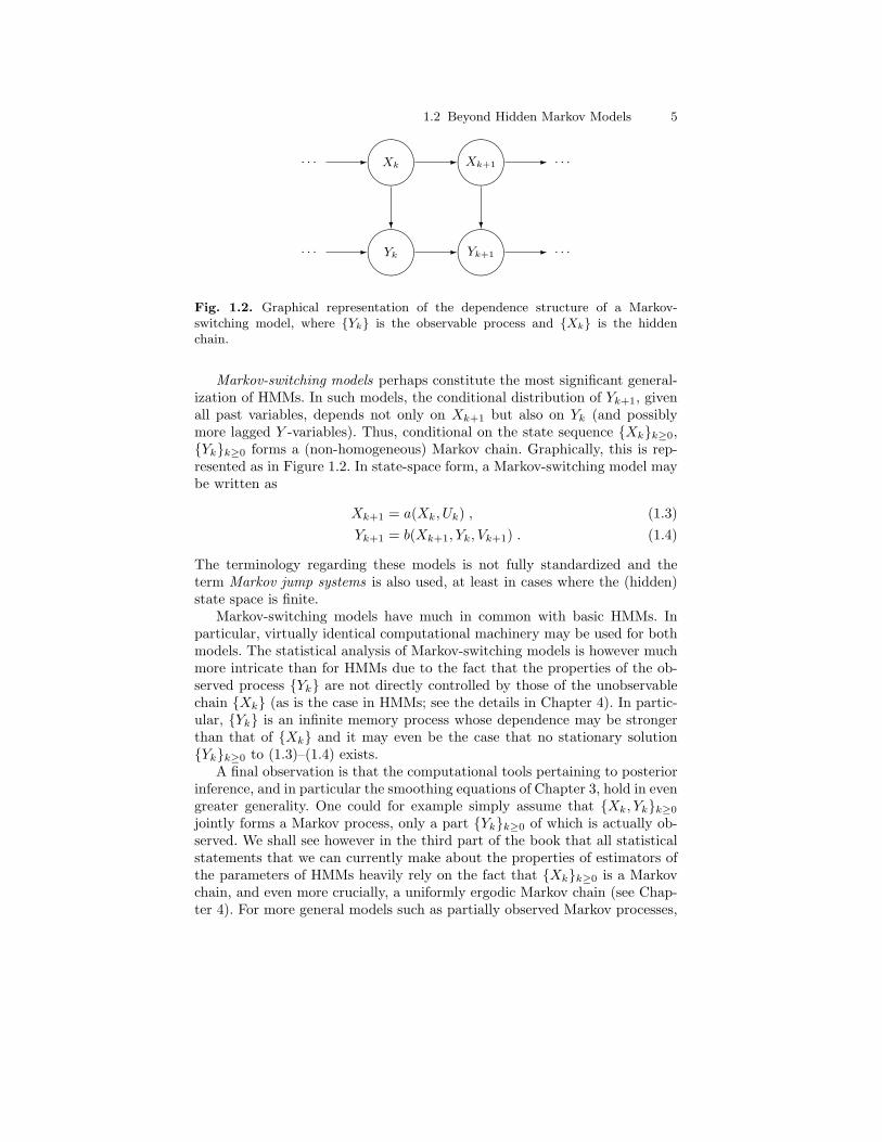
Fig. 1.2. Graphical representation of the dependence structure of a Markov-switching model, where Yk is the observable process and Xk is the hiddenchain.

Markov-switching models perhaps constitute the most significant general-ization of HMMs. In such models, the conditional distribution of Yk+1, givenall past variables, depends not only on Xk+1 but also on Yk (and possiblymore lagged Y -variables). Thus, conditional on the state sequence Xkk≥0,Ykk≥0 forms a (non-homogeneous) Markov chain. Graphically, this is rep-resented as in Figure 1.2. In state-space form, a Markov-switching model maybe written as

Xk+1 = a(Xk, Uk) , (1.3)Yk+1 = b(Xk+1, Yk, Vk+1) . (1.4)

The terminology regarding these models is not fully standardized and theterm Markov jump systems is also used, at least in cases where the (hidden)state space is finite.

Markov-switching models have much in common with basic HMMs. Inparticular, virtually identical computational machinery may be used for bothmodels. The statistical analysis of Markov-switching models is however muchmore intricate than for HMMs due to the fact that the properties of the ob-served process Yk are not directly controlled by those of the unobservablechain Xk (as is the case in HMMs; see the details in Chapter 4). In partic-ular, Yk is an infinite memory process whose dependence may be strongerthan that of Xk and it may even be the case that no stationary solutionYkk≥0 to (1.3)–(1.4) exists.

A final observation is that the computational tools pertaining to posteriorinference, and in particular the smoothing equations of Chapter 3, hold in evengreater generality. One could for example simply assume that Xk, Ykk≥0

jointly forms a Markov process, only a part Ykk≥0 of which is actually ob-served. We shall see however in the third part of the book that all statisticalstatements that we can currently make about the properties of estimators ofthe parameters of HMMs heavily rely on the fact that Xkk≥0 is a Markovchain, and even more crucially, a uniformly ergodic Markov chain (see Chap-ter 4). For more general models such as partially observed Markov processes,

6 1 Introduction

it is not yet clear what type of (not overly restrictive and reasonably general)conditions are required to guarantee that reasonable estimators (such as themaximum likelihood estimator for instance) are well behaved.

1.3 Examples

HMMs and their generalizations are nowadays used in many different areas.The (partial) bibliography by Cappe (2001b) (which contains more than 360references for the period 1990–2000) gives an idea of the reach of the do-main. Several specialized books are available that largely cover applications ofHMMs to some specific areas such as speech recognition (Rabiner and Juang,1993; Jelinek, 1997), econometrics (Hamilton, 1989; Kim and Nelson, 1999),computational biology (Durbin et al., 1998; Koski, 2001), or computer vision(Bunke and Caelli, 2001). We shall of course not try to compete with these infully describing real-world applications of HMMs. We will however considerthroughout the book a number of prototype HMMs (used in some of theseapplications) in order illustrate the variety of situations: finite-valued statespace (DNA or protein sequencing), binary Markov chain observed in Gaus-sian noise (ion channel), non-linear Gaussian state-space model (stochasticvolatility), conditionally Gaussian state-space model (deconvolution), etc.

It should be stressed that the idea one has about the nature of the hiddenMarkov chain Xk may be quite different from one case to another. In somecases it does have a well-defined physical meaning, whereas in other cases itis conceptually more diffuse, and in yet other cases the Markov chain maybe completely fictitious and the probabilistic structure of the HMM is thenused only as a tool for modeling dependence in data. These differences areillustrated in the examples below.

1.3.1 Finite Hidden Markov Models

In a finite hidden Markov model, both the state space X of the hidden Markovchain and the set Y in which the output lies are finite. We will generally assumethat these sets are 1, 2, . . . , r and 1, 2, . . . , s, respectively. The HMM isthen characterized by the transition probabilities qij = P(Xk+1 = j |Xk = i)of the Markov chain and the conditional probabilities gij = P(Yk = j |Xk = i).

Example 1.3.1 (Gilbert-Elliott Channel Model). The Gilbert-Elliottchannel model, after Gilbert (1960) and Elliott (1963), is used in informationtheory to model the occurrence of transmission errors in some digital commu-nication channels. Interestingly, this is a pre-HMM hidden Markov model, asit predates the seminal papers by Baum and his colleagues who introducedthe term hidden Markov model.

In digital communications, all signals to be transmitted are first digitizedand then transformed, a step known as source coding. After this preprocessing,

1.3 Examples 7

one can safely assume that the bits that represent the signal to be transmittedform an i.i.d. sequence of fair Bernoulli draws (Cover and Thomas, 1991). Wewill denote by Bkk≥0 the sequence of bits at the input of the transmissionsystem.

Abstracted high-level models of how this sequence of bits may get distortedduring the transmission are useful for devising efficient reception schemes andderiving performance bounds. The simplest model is the (memoryless) binarysymmetric channel in which it is assumed that each bit may be randomlyflipped by an independent error sequence,

Yk = Bk ⊕ Vk , (1.5)

where Ykk≥0 are the observations and Vkk≥0 is an i.i.d. Bernoulli sequencewith P(Vk = 1) = q, and ⊕ denotes modulo-two addition. Hence, the receivedbit is equal to the input bit Bk if Vk = 0; otherwise Yk 6= Bk and an erroroccurs.

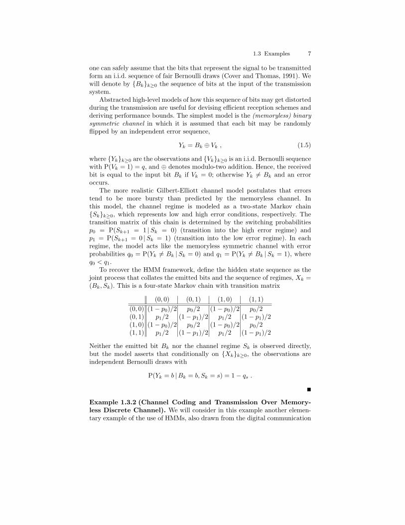
The more realistic Gilbert-Elliott channel model postulates that errorstend to be more bursty than predicted by the memoryless channel. Inthis model, the channel regime is modeled as a two-state Markov chainSkk≥0, which represents low and high error conditions, respectively. Thetransition matrix of this chain is determined by the switching probabilitiesp0 = P(Sk+1 = 1 |Sk = 0) (transition into the high error regime) andp1 = P(Sk+1 = 0 |Sk = 1) (transition into the low error regime). In eachregime, the model acts like the memoryless symmetric channel with errorprobabilities q0 = P(Yk 6= Bk |Sk = 0) and q1 = P(Yk 6= Bk |Sk = 1), whereq0 < q1.

To recover the HMM framework, define the hidden state sequence as thejoint process that collates the emitted bits and the sequence of regimes, Xk =(Bk, Sk). This is a four-state Markov chain with transition matrix

(0, 0) (0, 1) (1, 0) (1, 1)(0, 0) (1− p0)/2 p0/2 (1− p0)/2 p0/2(0, 1) p1/2 (1− p1)/2 p1/2 (1− p1)/2(1, 0) (1− p0)/2 p0/2 (1− p0)/2 p0/2(1, 1) p1/2 (1− p1)/2 p1/2 (1− p1)/2

Neither the emitted bit Bk nor the channel regime Sk is observed directly,but the model asserts that conditionally on Xkk≥0, the observations areindependent Bernoulli draws with

P(Yk = b |Bk = b, Sk = s) = 1− qs .

Example 1.3.2 (Channel Coding and Transmission Over Memory-less Discrete Channel). We will consider in this example another elemen-tary example of the use of HMMs, also drawn from the digital communication

8 1 Introduction

world. Assume we are willing to transmit a message encoded as a sequenceb0, . . . , bm of bits, where bi ∈ 0, 1 are the bits and m is the length of themessage. We wish to transmit this message over a channel, which will typicallyaffect the transmitted message by introducing (at random) errors.

To go further, we need to have an abstract model for the channel. In thisexample, we will consider discrete channels, that is, the channel’s inputs andoutputs are assumed to belong to finite alphabets: i1, . . . , iq for the inputsand o1, . . . , ol for the outputs. In this book, we will most often considerbinary channels only; then the inputs and the outputs of the transmissionchannel are bits, q = l = 2 and i1, i2 = o1, o2 = 0, 1. A transmissionchannel is said to be memoryless if the probability of the channel’s outputY0:n = y0:n conditional on its input sequence S0:n = s0:n factorizes as

P(Y0:n |S0:n) =n∏i=0

P(Yi |Si) .

In words, conditional on the input sequence S0:n, the channel outputs are con-ditionally independent. The transition probabilities of the discrete memory-less channel are defined by a transition kernel R : i1, . . . , iq×o1, . . . , ol →[0, 1], where for i = 1, . . . , q and j = 1, . . . , l,

R(ii, oj) = P(Y0 = oj |S0 = ii) . (1.6)

The most classical example of a discrete memoryless channel is the binarysymmetric channel (BSC) with binary input and binary output, for whichR(0, 1) = R(1, 0) = ε with ε ∈ [0, 1]. In words, every time a bit Sk = 0 or Sk =1 is sent across the BSC, the output is also a bit Yk = 0, 1, which differs fromthe input bit with probability ε; that is, the error probability is P(Yk 6= Ok) =ε. As described in Example 1.3.1, the output of a binary symmetric channelcan be modeled as a noisy version of the input sequence, Yk = Sk⊕Vk, where⊕ is the modulo-two addition and Vkk≥0 is an independent and identicallydistributed sequence of bits, independent of the input sequence Xkk≥0 andwith PVk = 0 = 1− ε. If we wish to transmit a message S0:m = b0:m over aBSC without coding, the probability of getting an error will be

P(Y0:m 6= b0:m |S0:m = b0:m) =1− P(Y0:m = b0:m |S0:m = b0:m) = 1− (1− ε)m .

Therefore, as m becomes large, with probability close to 1, at least one bitof the message will be incorrectly received, which calls for practical solution.Channel coding is a viable method to increase reliability, but at the expenseof reduced information rate. Increased reliability is achieved by adding redun-dancy to the information symbol vector, resulting in a longer coded vectorof symbols that are distinguishable at the output of the channel. There aremany ways to construct codes, and we consider in this example only a veryelementary example of a rate 1/2 convolutional coder with memory length 2.

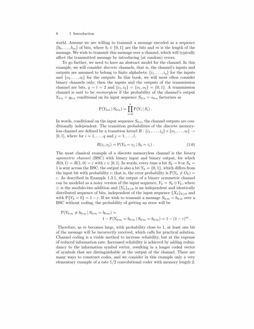
1.3 Examples 9

+

+

00100111

110000101011101000011101

1 0

Fig. 1.3. Rate 1/2 convolutional code with memory length 2.

The rate 1/2 means that a message of length m will be transformed into amessage of length 2m, that is, we will send 2m bits over the transmissionchannel in order to introduce some kind of redundancy to increase our chanceof getting an error-free message. The principle of this convolutional coder isdepicted in Figure 1.3.

Because the memory length is 2, there are 4 different states and the behav-ior of this convolutional encoder can be captured as 4-state machine, wherethe state alphabet is X = (0, 0), (0, 1), (1, 0), (1, 1). Denote by Xk the valueof the state at time k, Xk = (Xk,1, Xk,2) ∈ X. Upon the arrival of the bitBk+1, the state is transformed to

Xk+1 = (Xk+1,1, Xk+1,2) = (Bk+1, Xk,1) .

In the engineering literature, Xk is said to be a shift register. If the sequenceBkk≥0 of input bits is i.i.d. with probability P(Bk = 1) = p, then Xkk≥0

is a Markov chain with transition probabilities

P[Xk+1 = (1, 1) |Xk = (1, 0)] = P[Xk+1 = (1, 1) |Xk = (1, 1)] = p ,

P[Xk+1 = (1, 0) |Xk = (0, 1)] = P[Xk+1 = (1, 0) |Xk = (0, 0)] = p ,

P[Xk+1 = (0, 1) |Xk = (1, 0)] = P[Xk+1 = (0, 1) |Xk = (1, 1)] = 1− p ,P[Xk+1 = (0, 0) |Xk = (0, 1)] = P[Xk+1 = (0, 0) |Xk = (0, 0)] = 1− p ,

all other transition probabilities being zero. To each input bit, the convolu-tional encoder generates two outputs according to

Sk = (Sk,1, Sk,2) = (Bk ⊕Xk,2, Bk ⊕Xk,2 ⊕Xk,1) .

These encoded bits, referred to as symbols, are then sent on the transmissionchannel. A graphical interpretation of the problem is quite useful. A convo-lutional encoder (or, more generally, a finite state Markovian machine) canbe represented by a state transition diagram of the type in Figure 1.4. Thenodes are the states and the branches represent transitions having non-zeroprobability. If we index the states with both the time index k and state indexm, we get the trellis diagram of Figure 1.4. The trellis diagram shows the time

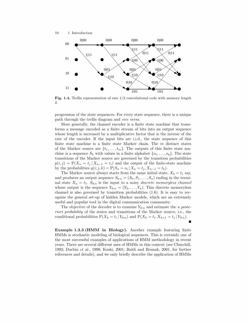
10 1 Introduction

1|10

00

01

10

11

1|11

0|00 0|00 0|00 0|00

1|11

1|11 1|11

0|01 0|010|01

1|001|00

1|10

0|11 0|11

1|01 1|01

0|100|10

1|10

Fig. 1.4. Trellis representation of rate 1/2 convolutional code with memory length2.

progression of the state sequences. For every state sequence, there is a uniquepath through the trellis diagram and vice versa.

More generally, the channel encoder is a finite state machine that trans-forms a message encoded as a finite stream of bits into an output sequencewhose length is increased by a multiplicative factor that is the inverse of therate of the encoder. If the input bits are i.i.d., the state sequence of thisfinite state machine is a finite state Markov chain. The m distinct statesof the Markov source are t1, . . . , tm. The outputs of this finite state ma-chine is a sequence Sk with values in a finite alphabet o1, . . . , oq. The statetransitions of the Markov source are governed by the transition probabilitiesp(i, j) = P(Xn = tj |Xn−1 = ti) and the output of the finite-state machineby the probabilities q(i; j, k) = P(Sn = oi |Xn = tj , Xn−1 = tk).

The Markov source always starts from the same initial state, X0 = t1 say,and produces an output sequence S0:n = (S0, S1, . . . , Sn) ending in the termi-nal state Xn = t1. S0:n is the input to a noisy discrete memoryless channelwhose output is the sequence Y0:n = (Y0, . . . , Yn). This discrete memorylesschannel is also governed by transition probabilities (1.6). It is easy to rec-ognize the general set-up of hidden Markov models, which are an extremelyuseful and popular tool in the digital communication community.

The objective of the decoder is to examine Y0:n and estimate the a poste-riori probability of the states and transitions of the Markov source, i.e., theconditional probabilities P(Xk = ti |Y0:n) and P(Xk = ti, Xk+1 = tj |Y0:n).

Example 1.3.3 (HMM in Biology). Another example featuring finiteHMMs is stochastic modeling of biological sequences. This is certainly one ofthe most successful examples of applications of HMM methodology in recentyears. There are several different uses of HMMs in this context (see Churchill,1992; Durbin et al., 1998; Koski, 2001; Baldi and Brunak, 2001, for furtherreferences and details), and we only briefly describe the application of HMMs

1.3 Examples 11

to gene finding in DNA, or more generally, functional annotation of sequencedgenomes.

In their genetic material, all living organisms carry a blueprint of themolecules they need for the complex task of living. This genetic materialis (usually) stored in the form of DNA—short for deoxyribonucleic acid—sequences. The DNA is not actually a sequence, but a long, chain-like moleculethat can be specified uniquely by listing the sequence of amine bases fromwhich it is composed. This process is known as sequencing and is a challengeon its own, although the number of complete sequenced genomes is growingat an impressive rate since the early 1990s. This motivates the abstract viewof DNA as a sequence over a four-letter alphabet A, C, G, and T (for adenine,cytosine, guanine, and thymine—the four possible instantiations of the aminebase).

The role of DNA is as a storage medium for information about the individ-ual molecules needed in the biochemical processes of the organism. A regionof the DNA that encodes a single functional molecule is referred to as a gene.Unfortunately, there is no easy way to discriminate coding regions (those thatcorrespond to genes) from non-coding ones. In addition, the dimension of theproblem is enormous as typical bacterial genomes can be millions of baseslong with the number of genes to be located ranging from a few hundreds toa few thousands.

The simplistic approach to this problem (Churchill, 1992) consists in mod-eling the observed sequence of bases Ykk≥0 ∈ A,C,G, T by a two-statehidden Markov model such that the non-observable state is binary-valued withone state corresponding to non-coding regions and the other one to coding re-gions. In the simplest form of the model, the conditional distribution of Ykgiven Xk is simply parameterized by the vector of probabilities of observing A,C, G, or T when in the coding and non-coding states, respectively. Despite itsdeceptive simplicity, the results obtained by estimating the parameters of thisbasic two-state finite HMM on actual genome sequences and then determin-ing the smoothed estimate of the state sequence Xk (using techniques to bediscussed in Chapter 3) were sufficiently promising to generate an importantresearch effort in this direction.

The basic strategy described above has been improved during the years toincorporate more and more of the knowledge accumulated about the behav-ior of actual genome sequences—see Krogh et al. (1994), Burges and Karlin(1997), Kukashin and Borodovsky (1998), Jarner et al. (2001) and referencestherein. A very important fact, for instance, is that in coding regions theDNA is structured into codons, which are composed of three successive sym-bols in our A, C, G, T alphabet. This property can be accommodated byusing higher order HMMs in which the distribution of Yk does not only de-pend on the current state Xk but also on the previous two observations Yk−1

and Yk−2. Another option consists in using non-homogeneous models suchthat the distribution of Yk does not only depend on the current state Xk

but also on the value of the index k modulo 3. In addition, some particular

12 1 Introduction

sub-sequences have a specific function, at least when they occur in a codingregion (there are start and end codons for instance). Needless to say, enlargingthe state space X to add specific states corresponding to those well identifiedfunctional sub-sequences is essential. Finally and most importantly, the func-tional description of the DNA sequence is certainly not restricted to just thecoding/non-coding dichotomy, and most models use many more hidden statesto differentiate between several distinct functional regions in the genome se-quence.

Example 1.3.4 (Capture-Recapture). Capture-recapture models are of-ten used in the study of populations with unknown sizes as in surveys, censusundercount, animal abundance evaluation, and software debugging to namea few of their numerous applications. To set up the model in its originalframework, we consider here the setting examined in Dupuis (1995) of a pop-ulation of lizards (Lacerta vivipara) that move between three spatially con-nected zones, denoted 1, 2, and 3, the focus being on modeling these moves.For a given lizard, the sequence of the zones where it stays can be modeledas a Markov chain with transition matrix Q. This model still pertains toHMMs as, at a given time, most lizards are not observed: this is therefore apartly hidden Markov model. To draw inference on the matrix Q, the capture-recapture experiment is run as follows. At time k = 0, a (random) numberof lizards are captured, marked, and released. This operation is repeated attimes k = 1, . . . , n by tagging the newly captured animals and by recordingat each capture the position (zone) of the recaptured animals. Therefore, themodel consists of a series of capture events and positions (conditional on acapture) of n+ 1 cohorts of animals marked at times k = 0, . . . , n. To accountfor open populations (as lizards can either die or leave the region of observa-tion for good), a fourth state is usually added to the three spatial zones. Itis denoted † (dagger) and, from the point of view of the underlying Markovchain, it is an absorbing state while, from the point of view of the HMM, itis always hidden.1

The observations may thus be summarized by the series Ykm0≤k≤n ofcapture histories that indicate, for each lizard at least captured once (m beingthe lizard index), in which zone it was at each of the times it was captured.We may for instance record

ykm0≤k≤n = (0, . . . , 0, 1, 1, 2, 0, 2, 0, 0, 3, 0, 0, 0, 1, 0, . . . , 0) ,

where 0 means that the lizard was not captured at that particular time in-dex. To each such observed sequence, there corresponds a (partially) hiddensequence Xkm0≤k≤n of lizard locations, for instance

xkm0≤k≤n = (1, . . . , 2,1,1,2,2,2,3, 2,3,3, 2, 2,1,†, . . . , †)1One could argue that lizards may also enter the population, either by migration

or by birth. The latter reason is easily accounted for, as the age of the lizard can beassessed at the first capture. The former reason is real but will be ignored.

1.3 Examples 13

which indicates that the animal disappeared right after the last capture (wherethe values that are deterministically known from the observations have beenstressed in bold).

The purposes in running capture-recapture experiments are often twofold:first, inference can be drawn on the size of the whole population based on therecapture history as in the Darroch model (Castledine, 1981; Seber, 1983),and, second, features of the population can be estimated from the capturedanimals, like capture and movement probabilities.

1.3.2 Normal Hidden Markov Models

By a normal hidden Markov model we mean an HMM in which the conditionaldistribution of Yk given Xk is Gaussian. In many applications, the state spaceis finite, and we will then assume it is 1, 2, . . . , r. In this case, given Xk = i,Yk ∼ N(µi, σ2

i ), so that the marginal distribution of Yk is a finite mixture ofnormals.

Example 1.3.5 (Ion Channel Modeling). A cell, for example in the hu-man body, needs to exchange various kinds of ions (sodium, potassium, etc.)with its surrounding for its metabolism and for purposes of chemical commu-nication. The cell membrane itself is impermeable to such ions but containsso-called ion channels, each tailored for a particular kind of ion, to let ionspass through. Such a channel is really a large molecule, a protein, that mayassume different configurations, or states. In some states, the channel allowsions to flow through—the channel is open—whereas in other states ions can-not pass—the channel is closed. A flow of ions is a transportation of electricalcharge, hence an electric current (of the order of picoamperes). In other words,each state of the channel is characterized by a certain conductance level. Theselevels may correspond to a fully open channel, a closed channel, or somethingin between. The current through the channel can be measured using specialprobes (this is by no means trivial!), with the result being a time series thatswitches between different levels as the channel reconfigures. In this context,the main motivation is to study the characteristics of the dynamic of these ionchannels, which is only partly understood, based on sampled measurements.

In the basic model, the channel current is simply assumed to be corruptedby additive white (i.i.d.) Gaussian measurement noise. If the state of the ionchannel is modeled as a Markov chain, the measured time series becomes anHMM with conditionally Gaussian output and with the variances σ2

i not de-pending on i. A limitation of this basic model is that if each physical configura-tion of the channel (say closed) corresponds to a single state of the underlyingMarkov chain, we are implicitly assuming that each visit to this state has aduration drawn from a geometric distribution. A work-around that makes itpossible to keep the HMM framework consists in modeling each physical con-figuration by a compound of distinct states of the underlying Markov chain,

14 1 Introduction

which are constrained to have a common conditional Gaussian output distri-bution. Depending on the exact transition matrix of the hidden chain, thedurations spent in a given physical configuration can be modeled by negativebinomial, mixtures of geometric or more complicated discrete distributions.

Further reading on ion-channel modeling can be found, for example, inBall and Rice (1992) for basic references and Ball et al. (1999) and Hodgson(1998) for more advanced statistical approaches.

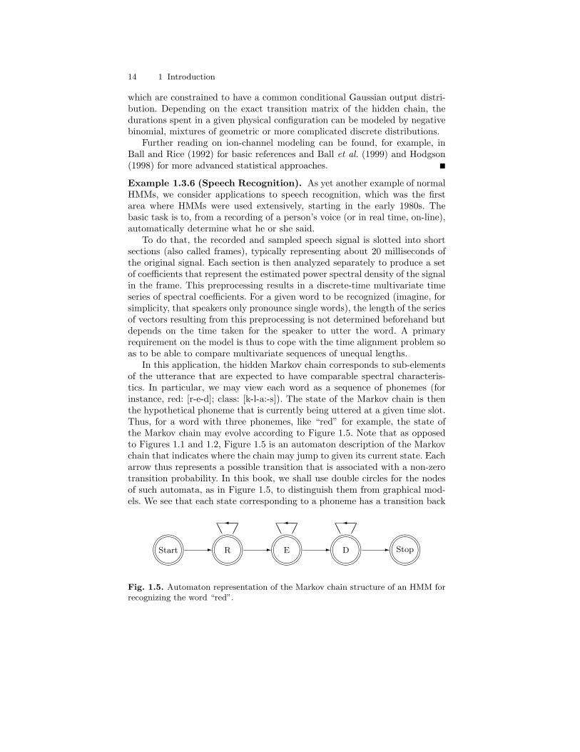
Example 1.3.6 (Speech Recognition). As yet another example of normalHMMs, we consider applications to speech recognition, which was the firstarea where HMMs were used extensively, starting in the early 1980s. Thebasic task is to, from a recording of a person’s voice (or in real time, on-line),automatically determine what he or she said.

To do that, the recorded and sampled speech signal is slotted into shortsections (also called frames), typically representing about 20 milliseconds ofthe original signal. Each section is then analyzed separately to produce a setof coefficients that represent the estimated power spectral density of the signalin the frame. This preprocessing results in a discrete-time multivariate timeseries of spectral coefficients. For a given word to be recognized (imagine, forsimplicity, that speakers only pronounce single words), the length of the seriesof vectors resulting from this preprocessing is not determined beforehand butdepends on the time taken for the speaker to utter the word. A primaryrequirement on the model is thus to cope with the time alignment problem soas to be able to compare multivariate sequences of unequal lengths.

In this application, the hidden Markov chain corresponds to sub-elementsof the utterance that are expected to have comparable spectral characteris-tics. In particular, we may view each word as a sequence of phonemes (forinstance, red: [r-e-d]; class: [k-l-a:-s]). The state of the Markov chain is thenthe hypothetical phoneme that is currently being uttered at a given time slot.Thus, for a word with three phonemes, like “red” for example, the state ofthe Markov chain may evolve according to Figure 1.5. Note that as opposedto Figures 1.1 and 1.2, Figure 1.5 is an automaton description of the Markovchain that indicates where the chain may jump to given its current state. Eacharrow thus represents a possible transition that is associated with a non-zerotransition probability. In this book, we shall use double circles for the nodesof such automata, as in Figure 1.5, to distinguish them from graphical mod-els. We see that each state corresponding to a phoneme has a transition back

- - - -

AA AA AA

Start R E D Stop

Fig. 1.5. Automaton representation of the Markov chain structure of an HMM forrecognizing the word “red”.

1.3 Examples 15

to itself, that is, a loop; this is to allow the phoneme to last for as long asthe recording of it does. The purposes of the initial state Start and termi-nal state Stop is simply to have well-defined starts and terminations of theMarkov chain; the stop state may be thought of as an absorbing state withno associated observation.

The observation vectors associated with a particular (unobservable) stateare assumed to be independent and are assigned a multivariate distribution,most often a mixture of Gaussian distributions. The variability induced by thisdistribution is used to model spectral variability within and between speak-ers. The actual speech recognition is realized by running the recorded wordas input to several different HMMs, each representing a particular word, andselecting the one that assigns the largest likelihood to the observed sequence.In a prior training phase, the parameters of each word model have been esti-mated using a large number of recorded utterances of the word. Note that theassociation of the states of the hidden chain with the phonemes in Figure 1.5is more a conceptual view than an actual description of what the model does.In practice, the recognition performance of HMM-based speech recognitionengines is far better than their efficiency at segmenting words into phonemes.

Further reading on speech recognition using HMMs can be found in thebooks by Rabiner and Juang (1993) and Jelinek (1997). The famous tutorialby Rabiner (1989) gives a more condensed description of the basic model, andYoung (1996) provides an overview of current large-scale speech recognitionsystems.

1.3.3 Gaussian Linear State-Space Models

The standard state-space model that we shall most often employ in this booktakes the form

Xk+1 = AXk +RUk , (1.7)Yk = BXk + SVk , (1.8)

where

• Ukk≥0, called the state or process noise, and Vkk≥0, called the mea-surement noise, are independent standard (multivariate) Gaussian whitenoise (sequences of i.i.d. multidimensional Gaussian random variables withzero mean and identity covariance matrices);

• The initial condition X0 is Gaussian with mean µν and covariance Γν andis uncorrelated with the processes Uk and Vk;

• The state transition matrix A, the measurement transition matrix B, thesquare-root of the state noise covariance R, and the square-root of themeasurement noise covariance S are known matrices with appropriate di-mensions.

16 1 Introduction

Ever since the pioneering work by Kalman and Bucy (1961), the study of theabove model has been a favorite both in the engineering (automatic control,signal processing) and time series literature. Recommended readings on thestate-space model include the books by Anderson and Moore (1979), Caines(1988), and Kailath et al. (2000). In addition to its practical importance,the Gaussian linear state-space model is interesting because it corresponds toone of the very few cases for which exact and reasonably efficient numericalprocedures are available to compute the distributions of the X-variables givenY -variables (see Chapters 3 and 5).

Remark 1.3.7. The form adopted for the model (1.7)–(1.8) is rather stan-dard (except for the symbols chosen for the various matrices, which varywidely in the literature), but the role of the matrices R and S deserve somecomments. We assume in the following that both noise sequences Uk andVk are i.i.d. with identity covariance matrices. Hence R and S serve assquare roots of the noise covariances, as

Cov(RUk) = RRt and Cov(SVk) = SSt ,

where the superscript t denotes matrix transposition. In some cases, and inparticular when either the X- or Y -variables are scalar, it would probablybe simpler to use U ′k = RUk and V ′k = SVk as noise variables, adoptingtheir respective covariance matrices as parameters of the model. In manysituations, however, the covariance matrices have a special structure that ismost naturally represented by using R and S as parameters. In Example 1.3.8below for instance, the dynamic noise vector Uk has a dimension much smallerthan that of the state vector Xk. Hence R is a tall matrix (with more rows thancolumns) and the covariance matrix of U ′k = RUk is rank deficient. It is thenmuch more natural to work only with the low-dimensional unit covariancedisturbance vector Uk rather than with U ′k = RUk. In the following, we willassume that SSt is a full rank covariance matrix (for reasons discussed inSection 5.2), but RRt will often be rank deficient as in Example 1.3.8.

In many respects, the case in which the state and measurement noises Ukand Vk are correlated is not much more complicated. It however departsfrom our usual assumptions in that Xk, Yk then forms a Markov chain butXk itself is no longer Markov. We will thus restrict ourselves to the casein which Uk and Vk are independent and refer, for instance, to Kailathet al. (2000) for further details on this issue.

Example 1.3.8 (Noisy Autoregressive Process). We shall define a pthorder scalar autoregressive (AR) process Zkk≥0 as one that satisfies thestochastic difference equation

Zk+1 = φ1Zk + · · ·+ φpZk−p+1 + Uk , (1.9)

where Ukk≥0 is white noise. Define the lag-vector

1.3 Examples 17

Xk = (Zk, . . . , Zk−p+1)t , (1.10)

and let A be the so-called companion matrix

A =

φ1 φ2 . . . φp1 0 . . . 00 1 . . . 0...

.... . .

...0 0 . . . 1 0

. (1.11)

Using these notations, (1.9) can be equivalently rewritten in state-space form:

Xk = AXk−1 +(1 0 . . . 0

)tUk−1 , (1.12)

Yk =(1 0 . . . 0

)Xk . (1.13)

If the autoregressive process is not directly observable but only a noisy versionof it is available, the measurement equation (1.13) is replaced by

Yk =(1 0 . . . 0

)Xk + Vk , (1.14)

where Vkk≥0 is the measurement noise. When there is no feedback betweenthe measurement noise and the autoregressive process, it is sensible to assumethat the state and measurement noises Uk and Vk are independent.

1.3.4 Conditionally Gaussian Linear State-Space Models

We gradually move toward more complicated models for which the state spaceX of the hidden chain is no more finite. The previous example is, as we shallsee in Chapter 5, a singular case because of the unique properties of themultivariate Gaussian distribution with respect to linear transformations. Wenow describe a related, although more complicated, situation in which thestate Xk is composed of two components Ck and Wk where the former is finite-valued whereas the latter is a continuous, possibly vector-valued, variable.The term “conditionally Gaussian linear state-space models”, or CGLSSMsin short, corresponds to structures by which the model, when conditioned onthe finite-valued process Ckk≥0, reduces to the form studied in the previoussection.

Conditionally Gaussian linear state-space models belong to a class of mod-els that we will refer to as hierarchical hidden Markov models, whose depen-dence structure is depicted in Figure 1.6. In such models the variable Ck, whichis the highest in the hierarchy, influences both the transition from Wk−1 toWk as well as the observation Yk. When Ck takes its values in a finite set,it is also common to refer to such models as jump Markov models, where thejumps correspond to the instants k at which the value of Ck differs from that ofCk−1. Of course, Figure 1.6 also corresponds to a standard HMM structure by

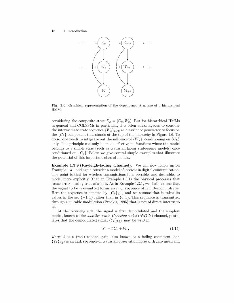
18 1 Introduction

· · · -

-

- · · ·Ck Ck+1

R R

? ?

· · · -

-

- · · ·Wk Wk+1

? ?

Yk Yk+1

Fig. 1.6. Graphical representation of the dependence structure of a hierarchicalHMM.

considering the composite state Xk = (Ck,Wk). But for hierarchical HMMsin general and CGLSSMs in particular, it is often advantageous to considerthe intermediate state sequence Wkk≥0 as a nuisance parameter to focus onthe Ck component that stands at the top of the hierarchy in Figure 1.6. Todo so, one needs to integrate out the influence of Wk, conditioning on Ckonly. This principle can only be made effective in situations where the modelbelongs to a simple class (such as Gaussian linear state-space models) onceconditioned on Ck. Below we give several simple examples that illustratethe potential of this important class of models.

Example 1.3.9 (Rayleigh-fading Channel). We will now follow up onExample 1.3.1 and again consider a model of interest in digital communication.The point is that for wireless transmissions it is possible, and desirable, tomodel more explicitly (than in Example 1.3.1) the physical processes thatcause errors during transmissions. As in Example 1.3.1, we shall assume thatthe signal to be transmitted forms an i.i.d. sequence of fair Bernoulli draws.Here the sequence is denoted by Ckk≥0 and we assume that it takes itsvalues in the set −1, 1 rather than in 0, 1. This sequence is transmittedthrough a suitable modulation (Proakis, 1995) that is not of direct interest tous.

At the receiving side, the signal is first demodulated and the simplestmodel, known as the additive white Gaussian noise (AWGN) channel, postu-lates that the demodulated signal Ykk≥0 may be written

Yk = hCk + Vk , (1.15)

where h is a (real) channel gain, also known as a fading coefficient, andVkk≥0 is an i.i.d. sequence of Gaussian observation noise with zero mean and

1.3 Examples 19

variance σ2. For reasons that are inessential for the discussion that follows,the actual model features complex channel gain and noise (Proakis, 1995), afact that we will ignore in the following.

The AWGN channel model ignores inter-symbol interference in the sensethat under (1.15) the observations Yk are i.i.d. In many practical situations,it is necessary to account for channel memory to obtain a reasonable modelof the received signal. Another issue is that, in particular in wireless commu-nication, the physical characteristics of the propagation path or channel arecontinuously changing over time. As a result, the fading coefficient h will typ-ically not stay constant but vary with time. A very simple model consists inassuming that the fading coefficient follows a (complex) autoregressive modelof order 1, giving the model

Wk+1 = ρWk + Uk ,

Yk = WkCk + Vk ,

where the time-varying h is denoted by Wk, and Ukk≥0 is white Gaussiannoise (an i.i.d. sequence of zero mean Gaussian random variables). With thismodel, it is easily checked that if we assume that W0 is a Gaussian randomvariable independent of both the observation noise Vk and the state noiseUk, Yk is the observation sequence corresponding to an HMM with hiddenstate Xk = (Ck,Wk) (the emitted bit and the fading coefficient). This is ageneral state-space HMM, as Wk is a real random variable. In this application,the aim is to estimate the sequence Ck of bits, which is thus a componentof the unobservable state sequence, given the observations Yk. The fadingcoefficients Wk are of no direct interest and constitute nuisance variables.

This model however has a unique feature among general state-space HMMsin that conditionally on the sequence Ck of bits, it reduces to a Gaussianlinear state-space model with state variables Wk. The only difference toSection 1.3.3 is that the observation equation becomes non-homogeneous intime,

Yk = Wkck + Vk ,

where Ck = ck is the event on which we are conditioning. As a strikingconsequence, we shall see in Chapters 4 and 5 that the distribution of Wk giventhe observations Y0, Y1, . . . , Yk is a mixture of 2k+1 Gaussian distributions.Because this is clearly not a tractable form when k is a two-digit number, thechallenge consists in finding practical approaches to approximate the exactdistributions.

Conditionally Gaussian models related to the previous example are alsocommonly used to approximate non-Gaussian state-space models. Imaginethat we are interested in the linear model given by Eqs. (1.7)–(1.8) with bothnoise sequences still being i.i.d. but at least one of them with a non-Gaussiandistribution. Assuming a very general form of the noise distribution woulddirectly lead us into the world of (general) continuous state-space HMMs. As

20 1 Introduction

a middle ground, we may however assume that the distribution of the noiseis a finite mixture of Gaussian distributions.

Let Ckk≥0 denote an i.i.d. sequence of random variables taking valuesin a set C, which can be finite or infinite. We refer to these variables asthe indicator variables when C is finite and latent variables otherwise. Tomodel non-Gaussian system dynamics we will typically replace the evolutionequation (1.7) by

Wk+1 = µW (Ck+1) +A(Ck+1)Wk +R(Ck+1)Uk , Uk ∼ N(0, I) ,

where, µW , A and R are respectively vector-valued and matrix-valued func-tions of suitable dimensions on C. When C = 1, . . . , r is finite, the distribu-tion of the noise µW (Ck+1) +R(Ck+1)Uk driving the state equation is a finitemixture of multivariate Gaussian distributions,

r∑i=1

mi N(µW (i), R(i)Rt(i)

)with mi = P(C0 = i) .

Another option consists in using the same modeling to represent non-Gaussianobservation noise by replacing the observation equation (1.8) by

Yk = µY (Ck) +B(Ck)Wk + S(Ck)Vk , Vk ∼ N(0, I) ,

where µY , B and S are respectively vector-valued and matrix-valued func-tions of suitable dimensions on C. Of course, by doing this the state of theHMM has to be extended to the joint process Xkk≥0, where Xk = (Wk, Ck),taking values in the product set X × C. At first sight, it is not obvious thatanything has been gained at all by introducing additional mixture indiceswith respect to our basic objective, which is to allow for linear state-spacemodels with non-Gaussian noises. We shall see however in Chapter 8 thatthe availability of computational procedures that evaluate quantities suchas E[Wk |Y0, . . . Yk, C0, . . . , Ck] is a distinct advantage of conditionally linearstate-space models over more general (unstructured) continuous state-spaceHMMs. Conditionally Gaussian linear state-space models (CGLSSM) havefound an exceptionally broad range of applications.

Example 1.3.10 (Change Point Detection). A simple yet useful exam-ple of CGLSSMs appears in change point detection problems (Shumway andStoffer, 1991; Fearnhead, 1998). In a Gaussian linear state-space model, thedynamics of the state depends on the state transition matrix and on the statenoise covariance. These quantities may change over time, and if the changes,when they occur, do so unannounced and at unknown time points, then theassociated inferential problem is referred to as a change point problem. Var-ious important application areas of statistics involve change detection in acentral way (for instance, environmental monitoring, quality assurance, bi-ology). In the simplest change point problem, the state variable is the level

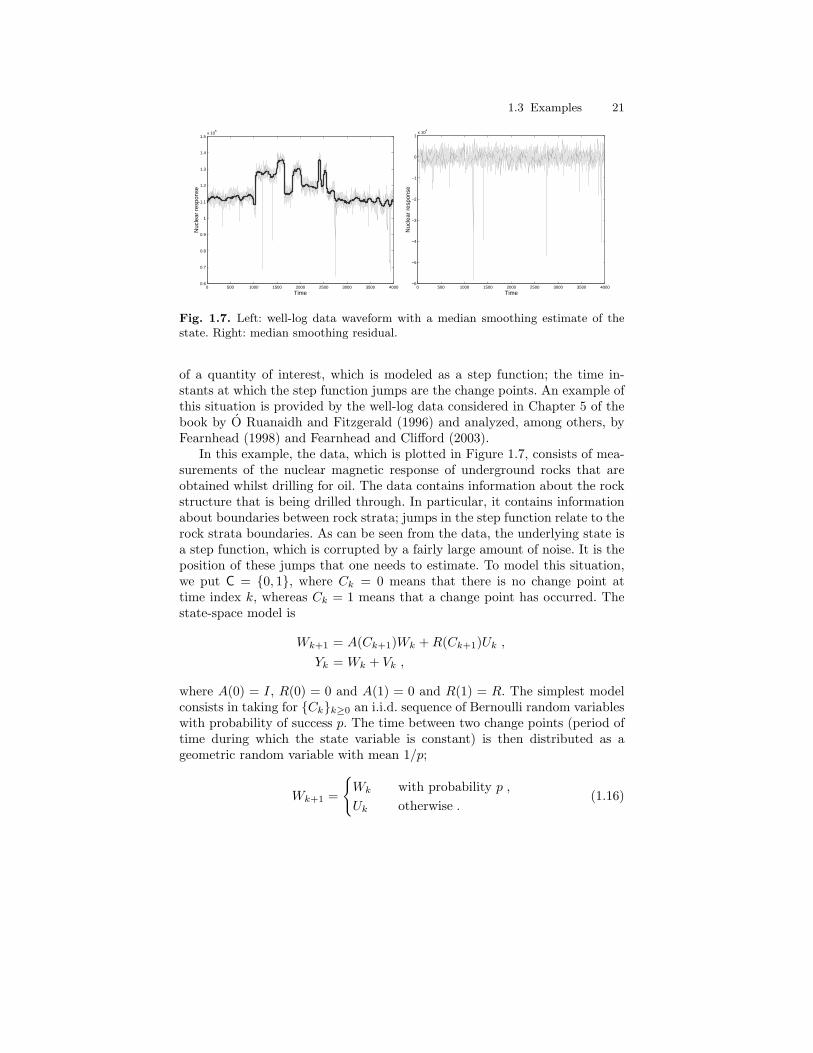
1.3 Examples 21

0 500 1000 1500 2000 2500 3000 3500 40000.6

0.7

0.8

0.9

1

1.1

1.2

1.3

1.4

1.5x 10

5

Time

Nuc

lear

res

pons

e

0 500 1000 1500 2000 2500 3000 3500 4000−6

−5

−4

−3

−2

−1

0

1x 10

4

Time

Nuc

lear

res

pons

e

Fig. 1.7. Left: well-log data waveform with a median smoothing estimate of thestate. Right: median smoothing residual.

of a quantity of interest, which is modeled as a step function; the time in-stants at which the step function jumps are the change points. An example ofthis situation is provided by the well-log data considered in Chapter 5 of thebook by O Ruanaidh and Fitzgerald (1996) and analyzed, among others, byFearnhead (1998) and Fearnhead and Clifford (2003).

In this example, the data, which is plotted in Figure 1.7, consists of mea-surements of the nuclear magnetic response of underground rocks that areobtained whilst drilling for oil. The data contains information about the rockstructure that is being drilled through. In particular, it contains informationabout boundaries between rock strata; jumps in the step function relate to therock strata boundaries. As can be seen from the data, the underlying state isa step function, which is corrupted by a fairly large amount of noise. It is theposition of these jumps that one needs to estimate. To model this situation,we put C = 0, 1, where Ck = 0 means that there is no change point attime index k, whereas Ck = 1 means that a change point has occurred. Thestate-space model is

Wk+1 = A(Ck+1)Wk +R(Ck+1)Uk ,Yk = Wk + Vk ,

where A(0) = I, R(0) = 0 and A(1) = 0 and R(1) = R. The simplest modelconsists in taking for Ckk≥0 an i.i.d. sequence of Bernoulli random variableswith probability of success p. The time between two change points (period oftime during which the state variable is constant) is then distributed as ageometric random variable with mean 1/p;

Wk+1 =

Wk with probability p ,Uk otherwise .

(1.16)

22 1 Introduction

It is possible to allow a more general form for the prior distribution of thedurations of the periods by introducing dependence among the indicator vari-ables.

Note that it is also possible to consider such multiple change point mod-els under the different, although strictly equivalent, perspective of a Bayesianmodel with an unknown number of parameters. In this alternative represen-tation, the hidden state trajectory is parameterized by the succession of itslevels (between two change points), which thus form a variable dimension setof parameters (Green, 1995; Lavielle and Lebarbier, 2001). Bayesian inferenceabout such parameters, equipped with a suitable prior distribution, is thencarried out using simulation-based techniques to be discussed further in Chap-ter 13.

Example 1.3.11 (Linear State-Space Model with Observational Out-liers and Heavy-Tailed Noise). Another interesting application of condi-tional Gaussian linear state-space models pertains to the field of robust statis-tics (Schick and Mitter, 1994). In the course of model building and validation,statisticians are often confronted with the problem of dealing with outliers.Routinely ignoring unusual observations is neither wise nor statistically sound,as such observations may contain valuable information about unmodeled sys-tem characteristics, model degradation and breakdown, measurement errorsand so forth.

The well-log data considered in the previous example illustrates this sit-uation. A visual inspection of the nuclear response reveals the presence ofoutliers, which tend to clump together in bursts (or clusters). This is con-firmed when plotting the quantile-quantile regression plot (see Figure 1.8)of the residuals of the well-log data obtained from a crude moving medianestimate of the state variable (the median filter applies a sliding window toa sequence and outputs the median value of all points in the window as asmoothed estimate at the window center). It can be seen that the normaldistribution does not fit the measurement noise well in the tails. FollowingFearnhead and Clifford (2003), we model the measurement noise as a mixtureof two Gaussian distributions. The model can be written

Wk+1 = A(Ck+1,1)Wk +R(Ck+1,1)Uk , Uk ∼ N(0, 1) ,Yk = µ(Ck,2) +B(Ck,2)Wk + S(Ck,2)Vk , Vk ∼ N(0, 1) ,

where Ck,1 ∈ 0, 1 and Ck,2 ∈ 0, 1 are indicators of a change point and ofthe presence of an outlier, respectively. As above, the level is assumed to beconstant between two change points. Therefore we put A(0) = 1, R(0) = 0,A(1) = 0, and R(1) = σU . When there is no outlier, that is, Ck,2 = 0,we assume that the level is observed in additive Gaussian noise. Thereforeµ(0), B(0), S(0) = (0, 1, σV,0). In the presence of an outlier, the measure-ment does no longer carry information about the current value of the level,that is, B(1) = 0, and the measurement noise is assumed to follow a Gaus-sian distribution with negative mean µ and (large) variance σV,1. Therefore

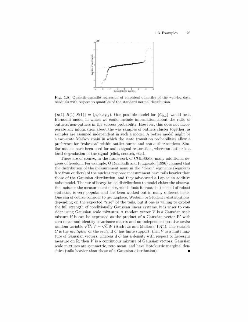
1.3 Examples 23

−4 −3 −2 −1 0 1 2 3 4−6

−4

−2

0

2

4

6x 10

4

Standard Normal QuantilesQ

uant

iles

of In

put S

ampl

e

Fig. 1.8. Quantile-quantile regression of empirical quantiles of the well-log dataresiduals with respect to quantiles of the standard normal distribution.

µ(1), B(1), S(1) = (µ, 0, σV,1). One possible model for Ck,2 would be aBernoulli model in which we could include information about the ratio ofoutliers/non-outliers in the success probability. However, this does not incor-porate any information about the way samples of outliers cluster together, assamples are assumed independent in such a model. A better model might bea two-state Markov chain in which the state transition probabilities allow apreference for “cohesion” within outlier bursts and non-outlier sections. Sim-ilar models have been used for audio signal restoration, where an outlier is alocal degradation of the signal (click, scratch, etc.).

There are of course, in the framework of CGLSSMs, many additional de-grees of freedom. For example, O Ruanaidh and Fitzgerald (1996) claimed thatthe distribution of the measurement noise in the “clean” segments (segmentsfree from outliers) of the nuclear response measurement have tails heavier thanthose of the Gaussian distribution, and they advocated a Laplacian additivenoise model. The use of heavy-tailed distributions to model either the observa-tion noise or the measurement noise, which finds its roots in the field of robuststatistics, is very popular and has been worked out in many different fields.One can of course consider to use Laplace, Weibull, or Student t-distributions,depending on the expected “size” of the tails, but if one is willing to exploitthe full strength of conditionally Gaussian linear systems, it is wiser to con-sider using Gaussian scale mixtures. A random vector V is a Gaussian scalemixture if it can be expressed as the product of a Gaussian vector W withzero mean and identity covariance matrix and an independent positive scalarrandom variable

√C: V =

√CW (Andrews and Mallows, 1974). The variable

C is the multiplier or the scale. If C has finite support, then V is a finite mix-ture of Gaussian vectors, whereas if C has a density with respect to Lebesguemeasure on R, then V is a continuous mixture of Gaussian vectors. Gaussianscale mixtures are symmetric, zero mean, and have leptokurtic marginal den-sities (tails heavier than those of a Gaussian distribution).

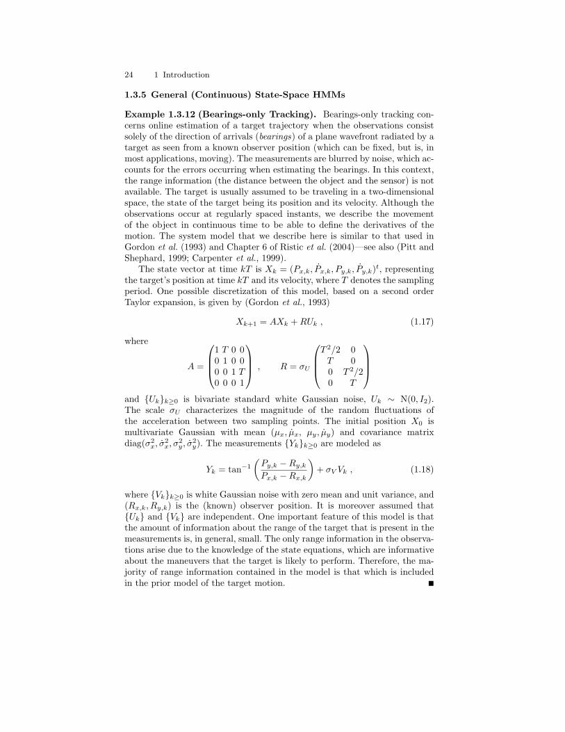
24 1 Introduction

1.3.5 General (Continuous) State-Space HMMs

Example 1.3.12 (Bearings-only Tracking). Bearings-only tracking con-cerns online estimation of a target trajectory when the observations consistsolely of the direction of arrivals (bearings) of a plane wavefront radiated by atarget as seen from a known observer position (which can be fixed, but is, inmost applications, moving). The measurements are blurred by noise, which ac-counts for the errors occurring when estimating the bearings. In this context,the range information (the distance between the object and the sensor) is notavailable. The target is usually assumed to be traveling in a two-dimensionalspace, the state of the target being its position and its velocity. Although theobservations occur at regularly spaced instants, we describe the movementof the object in continuous time to be able to define the derivatives of themotion. The system model that we describe here is similar to that used inGordon et al. (1993) and Chapter 6 of Ristic et al. (2004)—see also (Pitt andShephard, 1999; Carpenter et al., 1999).

The state vector at time kT is Xk = (Px,k, Px,k, Py,k, Py,k)t, representingthe target’s position at time kT and its velocity, where T denotes the samplingperiod. One possible discretization of this model, based on a second orderTaylor expansion, is given by (Gordon et al., 1993)

Xk+1 = AXk +RUk , (1.17)

where

A =

1 T 0 00 1 0 00 0 1 T0 0 0 1

, R = σU

T 2/2 0T 00 T 2/20 T

and Ukk≥0 is bivariate standard white Gaussian noise, Uk ∼ N(0, I2).The scale σU characterizes the magnitude of the random fluctuations ofthe acceleration between two sampling points. The initial position X0 ismultivariate Gaussian with mean (µx, µx, µy, µy) and covariance matrixdiag(σ2

x, σ2x, σ

2y, σ

2y). The measurements Ykk≥0 are modeled as

Yk = tan−1

(Py,k −Ry,kPx,k −Rx,k

)+ σV Vk , (1.18)

where Vkk≥0 is white Gaussian noise with zero mean and unit variance, and(Rx,k, Ry,k) is the (known) observer position. It is moreover assumed thatUk and Vk are independent. One important feature of this model is thatthe amount of information about the range of the target that is present in themeasurements is, in general, small. The only range information in the observa-tions arise due to the knowledge of the state equations, which are informativeabout the maneuvers that the target is likely to perform. Therefore, the ma-jority of range information contained in the model is that which is includedin the prior model of the target motion.

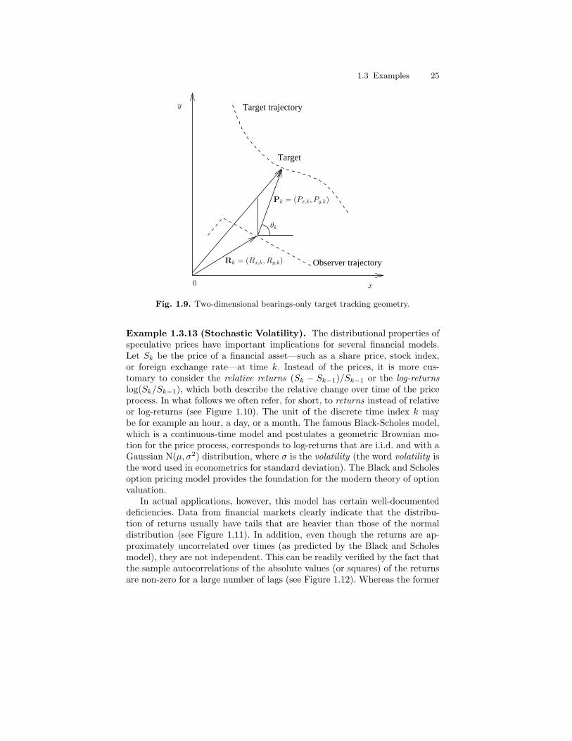
1.3 Examples 25

Target trajectory

Target

Observer trajectory

0 x

y

θk

Pk = (Px,k, Py,k)

Rk = (Rx,k, Ry,k)

Fig. 1.9. Two-dimensional bearings-only target tracking geometry.

Example 1.3.13 (Stochastic Volatility). The distributional properties ofspeculative prices have important implications for several financial models.Let Sk be the price of a financial asset—such as a share price, stock index,or foreign exchange rate—at time k. Instead of the prices, it is more cus-tomary to consider the relative returns (Sk − Sk−1)/Sk−1 or the log-returnslog(Sk/Sk−1), which both describe the relative change over time of the priceprocess. In what follows we often refer, for short, to returns instead of relativeor log-returns (see Figure 1.10). The unit of the discrete time index k maybe for example an hour, a day, or a month. The famous Black-Scholes model,which is a continuous-time model and postulates a geometric Brownian mo-tion for the price process, corresponds to log-returns that are i.i.d. and with aGaussian N(µ, σ2) distribution, where σ is the volatility (the word volatility isthe word used in econometrics for standard deviation). The Black and Scholesoption pricing model provides the foundation for the modern theory of optionvaluation.

In actual applications, however, this model has certain well-documenteddeficiencies. Data from financial markets clearly indicate that the distribu-tion of returns usually have tails that are heavier than those of the normaldistribution (see Figure 1.11). In addition, even though the returns are ap-proximately uncorrelated over times (as predicted by the Black and Scholesmodel), they are not independent. This can be readily verified by the fact thatthe sample autocorrelations of the absolute values (or squares) of the returnsare non-zero for a large number of lags (see Figure 1.12). Whereas the former

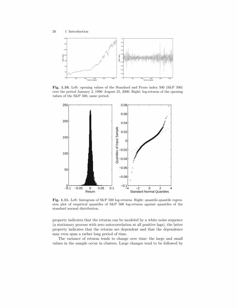
26 1 Introduction

0 500 1000 1500 2000 2500200

400

600

800

1000

1200

1400

1600

Time (in days)

S&

P In

dex

0 500 1000 1500 2000 2500−0.1

−0.08

−0.06

−0.04

−0.02

0

0.02

0.04

0.06

0.08

0.1

Time (in days)

S&

P In

dex

Fig. 1.10. Left: opening values of the Standard and Poors index 500 (S&P 500)over the period January 2, 1990–August 25, 2000. Right: log-returns of the openingvalues of the S&P 500, same period.

−0.1 −0.05 0 0.05 0.10

50

100

150

200

250

Return−4 −2 0 2 4

−0.1

−0.08

−0.06

−0.04

−0.02

0

0.02

0.04

0.06

0.08

Standard Normal Quantiles

Qua

ntile

s of

Inpu

t Sam

ple

Fig. 1.11. Left: histogram of S&P 500 log-returns. Right: quantile-quantile regres-sion plot of empirical quantiles of S&P 500 log-returns against quantiles of thestandard normal distribution.

property indicates that the returns can be modeled by a white noise sequence(a stationary process with zero autocorrelation at all positive lags), the latterproperty indicates that the returns are dependent and that the dependencemay even span a rather long period of time.

The variance of returns tends to change over time: the large and smallvalues in the sample occur in clusters. Large changes tend to be followed by

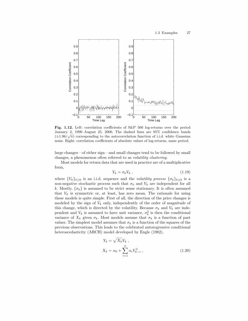
1.3 Examples 27

0 50 100 150 200−0.1

0

0.1

0.2

0.3

0.4

0.5

0.6

0.7

0.8

0.9

Time Lag

Cor

rela

tion

Coe

ffici

ent

0 50 100 150 200−0.1

0

0.1

0.2

0.3

0.4

0.5

0.6

0.7

0.8

0.9

Time Lag

Cor

rela

tion

Coe

ffici

ent

Fig. 1.12. Left: correlation coefficients of S&P 500 log-returns over the periodJanuary 2, 1990–August 25, 2000. The dashed lines are 95% confidence bands(±1.96/

√n) corresponding to the autocorrelation function of i.i.d. white Gaussian

noise. Right: correlation coefficients of absolute values of log-returns, same period.

large changes—of either sign—and small changes tend to be followed by smallchanges, a phenomenon often referred to as volatility clustering.

Most models for return data that are used in practice are of a multiplicativeform,

Yk = σkVk , (1.19)

where Vkk≥0 is an i.i.d. sequence and the volatility process σkk≥0 is anon-negative stochastic process such that σk and Vk are independent for allk. Mostly, σk is assumed to be strict sense stationary. It is often assumedthat Vk is symmetric or, at least, has zero mean. The rationale for usingthese models is quite simple. First of all, the direction of the price changes ismodeled by the sign of Vk only, independently of the order of magnitude ofthis change, which is directed by the volatility. Because σk and Vk are inde-pendent and Vk is assumed to have unit variance, σ2

k is then the conditionalvariance of Xk given σk. Most models assume that σk is a function of pastvalues. The simplest model assumes that σk is a function of the squares of theprevious observations. This leads to the celebrated autoregressive conditionalheteroscedasticity (ARCH) model developed by Engle (1982),

Yk =√XkVk ,

Xk = α0 +p∑i=1

αiY2k−i , (1.20)

28 1 Introduction

where α0, . . . , αp are non-negative constants. In the Engle (1982) model, Vkis normal; hence the conditional error distribution is normal, but with con-ditional variance equal to a linear function of the p past squared observa-tions. ARCH models are thus able to reproduce the tendency for extremevalues to be followed by other extreme values, but of unpredictable sign.The autoregressive structure can be seen by the following argument. Writ-ing νk = Y 2

k −Xk = Xk(V 2k − 1), one obtains

Y 2k −

p∑i=1

αiY2k−i = α0 + νk . (1.21)

Because Vk is an i.i.d. sequence with zero mean and unit variance, νkk≥0

is an uncorrelated sequence. Because ARCH(p) processes do not fit log-returnsvery well unless the order p is quite large, various people have thought aboutimprovements. As (1.21) bears some resemblance to an AR structure, a possi-ble generalization is to introduce an ARMA structure. This construction leadsto the so-called GARCH(p, q) process (Bollerslev et al., 1994). This model dis-plays some striking similarities to autoregressive models with Markov regime;this will be discussed in more detail below.

An alternative to the ARCH/GARCH framework is a model in which thevariance is specified to follow some latent stochastic process. Such models,referred to as stochastic volatility (SV) models, appear in the theoretical lit-erature on option pricing and exchange rate modeling. In contrast to GARCH-type processes, there is no direct feedback from past returns to the volatilityprocess, which has been questioned as unnatural by some authors. Empiri-cal versions of the SV model are typically formulated in discrete time, whichmakes inference problems easier to deal with. The canonical model in SV fordiscrete-time data is (Hull and White, 1987; Jacquier et al., 1994),

Xk+1 = φXk + σUk , Uk ∼ N(0, 1) ,Yk = β exp(Xk/2)Vk , Vk ∼ N(0, 1) , (1.22)

where the observations Ykk≥0 are the log-returns, Xkk≥0 is the log-volatility, which is assumed to follow a stationary autoregression of order1, and Ukk≥0 and Vkk≥0 are independent i.i.d. sequences. The parameterβ plays the role of the constant scaling factor, φ is the persistence (mem-ory) in the volatility, and σ is the volatility of the log-volatility. Despite avery parsimonious representation, this model is capable of exhibiting a widerange of behaviors. Like ARCH/GARCH models, the model can give rise toa high persistence in volatility (“volatility clustering”). Even with φ = 0, themodel is a Gaussian scale mixture that will give rise to excess kurtosis in themarginal distribution of the data. In ARCH/GARCH models with normal er-rors, the degree of kurtosis is tied to the roots of the volatility equation; as thevolatility becomes more correlated, the degree of kurtosis also increases. Inthe stochastic volatility model, the parameter σ governs the degree of mixingindependently of the degree of smoothness in the variance evolution.

1.3 Examples 29

It is interesting to note that stochastic volatility models are related toconditionally Gaussian linear state-space models. By taking logarithms of thesquared returns, one obtains,

Xk = φXk−1 + σUk−1 ,

log Y 2k = log β2 +Xk + Zk , where Zk = log V 2

k .

If Vk is standard normal, Zk follows the logχ21 distribution. This distribution

may be approximated with arbitrary accuracy by a finite mixture of Gaussiandistributions, and then the SV model becomes a conditionally Gaussian linearstate-space model (Sandmann and Koopman, 1998; Durbin and Koopman,2000). This time, the latent variable Ck is the mixture component and themodel writes

Wk+1 = φWk + Uk , Uk ∼ N(0, 1) ,Yk = Wk + (µ(Ck) + σV (Ck)Vk) , Vk ∼ N(0, 1) .

This representation of the stochastic volatility model may prove useful whenderiving numerical algorithms to filter the hidden state or estimate the modelparameters.

1.3.6 Switching Processes with Markov Regime

We now consider several examples that are not HMMs but belong to the classof Markov-switching models already mentioned in Section 1.2. Perhaps themost famous example of Markov-switching processes is the switching autore-gressive process that was introduced by Hamilton (1989) to model econometricdata.

1.3.6.1 Switching Linear Models

A switching linear autoregression is a model of the form

Yk = µ(Ck) +d∑i=1

ai(Ck)(Yk−i − µ(Ck−i) + σ(Ck)Vk , k ≥ 1 , (1.23)

where Ckk≥0, called the regime, is a Markov chain on a finite state spaceC = 1, 2, . . . , r, and Vkk≥0 is white noise independent of the regime; thefunctions µ : C → R, ai : C → R, i = 1, . . . , r, and σ : C → R describethe dependence of the parameters on the realized regime. In this model, wechange only the scale of the innovation as a function of the regime, but wecan of course more drastically change the innovation distribution conditionalon each state.

30 1 Introduction

Remark 1.3.14. A model closely related to (1.23) is

Yk = µ(Ck) +d∑i=1

ai(Ck)Yk−i + σ(Ck)Vk , k ≥ 1 . (1.24)

In (1.23), µ(Ck) is the mean of Yk conditional on the sequence of statesC1, . . . , Ck, whereas in (1.24) the shift is on the intercept of the autoregressiveprocess.

A model like this is not an HMM because, given Ck, the Yk are notconditionally independent but rather form a non-homogeneous autoregression.Hence it is a Markov-switching model. Obviously, the conditional distributionof Yk does not only depend on Ck and Yk−1 but also on other lagged Cs andY s back to Ck−d and Yk−d. By vectorizing the Y s and Cs, that is, stackingthem in groups of d elements, we can obtain a process whose conditionaldistribution depends on one lagged variable only, as in Figure 1.2.

This model can be rewritten in state-space form. Let

Yk = [Yk, Yk−1, . . . , Yk−d+1]t ,

Ck = [Ck, Ck−1, . . . , Ck−d+1]t ,

µ(Ck) = [µ(Ck), . . . , µ(Ck−d+1)]t ,

Vk = [Vk, 0, . . . , 0]t ,

and denote by C(c) the d × d companion matrix associated with the autore-gressive coefficients of the state c,

A(c) =

a1(c) a2(c) . . . . . . ad(c)1 0 0

0 1 0...

.... . . . . . . . .

...0 . . . 0 1 0

. (1.25)

The stacked observation vector Yk then satisfies

Yk = µ(Ck) +A(Ck) (Yk−1 − µ(Ck−1)) + σ(Ck)Vk . (1.26)

Interestingly enough, switching autoregressive processes have a rather richprobabilistic structure and have proven to be useful in many different contexts.We focus here on applications in econometrics and finance, but the scope ofpotential applications of these models span many different areas.

Example 1.3.15 (Regime Switches in Econometrics). The Hamilton(1989) model for the U.S. business cycle fostered a great deal of interest inMarkov-switching autoregressive models as an empirical vehicle for character-izing macro-economic fluctuations. This model provides a formal statistical

1.3 Examples 31

representation of the old idea that expansion and contraction constitute twodistinct economic phases: Hamilton’s model assumes that a macro-economicaggregate (real output growth, country’s gross national product measured perquarter, annum, etc.) follows one of two different autoregressions dependingon whether the economy is expanding or contracting, with the shift betweenregimes governed by the outcome of an unobserved Markov chain. The simplebusiness cycle model advocated by Hamilton takes the form

Yk = µ(Ck) +d∑i=1

ai(Yk−i − µ(Ck−i)) + σVk , (1.27)

where Vkk≥0 is white Gaussian noise with zero mean and unit variance,and Ckk≥0 is the unobserved latent variable that reflects the state of thebusiness cycle (the autoregressive coefficients do not change; only the meanof the process is effectively modulated). In the simplest model, Ck takesonly two values; for example, Ck = 0 could indicate that the economy is inrecession and Ck = 1 that it is in expansion. When Ck = 0, the average growthrate is given by µ(0), whereas when Ck = 1 the average growth rate is µ(1).This simple model can be made more sophisticated by making the variance afunction of the state Ck as well,

Yk = µ(Ck) +d∑i=1

ai(Yk−i − µ(Ck−i)) + σ(Ck)Vk .

The Markov assumption on the hidden states basically says that if the econ-omy was, say, in expansion the last period, the probability of going into re-cession is a fixed constant that does not depend on how long the economy hasbeen in expansion or other measures of the strength of the expansion. Thisassumption, though rather naive, does not appear to be a bad representationof historical experience, though several researchers have suggested that morecomplicated specifications of the transition matrix ought to be considered.

Further reading on applications of switching linear Gaussian autoregres-sions in economics and finance can be found in, for instance, Krolzig (1997),Kim and Nelson (1999), Raj (2002), and Hamilton and Raj (2003).

It is possible to include an additional degree of sophistication by consid-ering instead of a linear autoregression, linear state-space models (see for in-stance Tugnait, 1984; West and Harrison, 1989; Kim and Nelson, 1999; Doucetet al., 2000a; Chen and Liu, 2000):

Wk+1 = µW (Ck+1) +A(Ck+1)Wk +R(Ck+1)Uk ,Yk = µY (Ck) +B(Ck)Wk + S(Ck)Vk , (1.28)

where Ckk≥0 is a Markov chain on a discrete state space, Ukk≥0 andVkk≥0 are mutually independent i.i.d. sequences independent of Ckk≥0,

32 1 Introduction

and µW , µY , A, B, R, and S are vector- and matrix-valued functions of ap-propriate dimensions. Each state of the underlying Markov chain is then asso-ciated with a particular regime of the dynamic system, specified by particularvalues of (µW , µY , A,B,R, S) governing the behavior the state and observa-tions. Switching linear state-space models approximate complex non-lineardynamics with a dynamic mixture of linear processes. This type of modelhas found a broad range of applications in econometrics (Kim and Nelson,1999), in engineering including control (hybrid system, target tracking), sig-nal processing (blind channel equalization) and communications (interferencesuppression) (Doucet et al., 2000b, 2001b).

Example 1.3.16 (Maneuvering Target). Recall that in Example 1.3.12,we considered the motion of a single target that evolves in 2-D space with(almost) constant velocity. To represent changes in the velocity (either speedor direction or both), we redefine the model that describes the evolution of thestate Wk = (Px,k, Px,k, Py,k, Py,k) by making it conditional upon a maneuverindicator Ck = ck ∈ 1, . . . , r that is assumed to take only a finite numberof values corresponding to various predefined maneuver scenarios. The statenow evolves according to the following conditionally Gaussian linear equation

Wk = A(Ck+1)Wk +R(Ck+1)Uk , Uk ∼ N(0, I) ,

where A(c) and R(c) describe the parameters of the dynamic system char-acterizing the motion of the target for the maneuver labeled by c. Assumingthat the observations are linear, Yk = BWk + Vk, the system is a switchingGaussian linear state-space model.

1.3.6.2 Switching Non-linear Models

Switching autoregressive processes with Markov regime can be generalized byallowing non-linear autoregressions. Such models were considered in particularby Francq and Roussignol (1997) and take the form

Yk = φ(Yk−1, . . . , Yk−d, Xk) + σ(Yk−1, . . . , Yk−d, Xk)Vk , (1.29)

where Xkk≥0, called the regime, is a Markov chain on a discrete state spaceX, Vk is an i.i.d. sequence, independent of the regime, with zero mean andunit variance, and φ : Rd×X→ R and σ : Rd×X→ R+ are (measurable) func-tions. Of particular interest are the switching ARCH models (Francq et al.,2001),

Yk =√ζ0(Xk) + ξ1(Xk)Y 2

t−1 + ξd(Xk)Y 2t−d Vk .

Krishnamurthy and Ryden (1998) studied an even more general class ofswitching autoregressive processes that do not necessarily admit an additivedecomposition; these are characterized by

Yk = φ(Yk−1, . . . , Yk−d, Xk, Vk) , (1.30)

1.4 Left-to-Right and Ergodic Hidden Markov Models 33

where Xkk≥0, the regime, is a Markov chain on a discrete state space,Vkk≥0 is an i.i.d. sequence independent of the regime, and φ : Rd × X→ Ris a (measurable) function. Conditional on the regime, Yk is thus a dth orderMarkov chain on a general state space. Douc et al. (2004) studied the samekind of model but allowing the regime to evolve on a general state space.

Example 1.3.17 (Switching ARCH Models). Hamilton’s (1989) switch-ing autoregression (1.27) models a change in the business cycle phase as ashift in the average growth rate. By contrast, Hamilton and Susmel (1994)modeled changes in the volatility of the stock market as a shift in the overallscale of the ARCH process modeling stock returns. They suggested to modelthe monthly excess return of a financial asset (for example, the excess returnof a financial index over the treasury bill yield) as

Wk =√ζ0 + ξ1W 2

k−1 + · · ·+ ξmW 2k−mUk ,

Yk = δ0 + δ1Yk−1 + · · ·+ δqYk−q + σ(Ck)Wk . (1.31)

where Ukk≥0 is Gaussian white noise with zero mean and Ckk≥0 is an un-observed Markov chain on a discrete state space that represents the volatilityphase of the stock market; Ck and Uk are independent. In the absence ofsuch phases, the parameter σ(Ck) would simply be constant over k, and (1.31)would describe stock returns by an autoregressive model whose innovationsUk follow an mth order ARCH process.

More generally, when the function σ : C → R+ is not identically equalto unity, the latent ARCH process Wk is multiplied by a scale factor σ(Ck)representing the current phase Ck that characterizes overall stock volatility.Assuming again that the market has two phases, C = 0, 1, and normalizingσ(0) = 1, σ(1) has the interpretation as the ratio of the average variance ofstock returns when Ck = 1 compared to that observed when Ck = 0.

1.4 Left-to-Right and Ergodic Hidden Markov Models

Most HMMs fall into one of two principally different classes of models: left-to-right HMMs and ergodic HMMs. By a left-to-right HMM is meant an HMMwith a Markov chain that starts in a particular initial state, traverses a numberof intermediate states, and finally terminates in a final state (this state may beconsidered as absorbing). When traversing the intermediate states the chainmay not go backwards—toward the initial state—but only toward the finalstate. This progression is usually pictured from left to right; thus the term“left-to-right HMM”. Speech recognition, discussed in Example 1.3.6 above, istypically a case where only left-to-right HMMs are used. A left-to-right HMMis not ergodic, but produces a sequence, typically of random length, of output.The number of states is also usually large.

34 1 Introduction

In contrast, an ergodic HMM is one for which the underlying Markov chainis ergodic, or at least is irreducible and admits a unique stationary distribution(thus allowing for periodicity). Such a model can thus produce an infinitelylong sequence of output, which is an ergodic sequence as well. The numberof states, if the state space is finite, is typically small. Most of the examplesmentioned in Section 1.3 correspond to ergodic HMMs.

Left-to-right HMMs and ergodic HMMs have much in common, in par-ticular on the computational side. Indeed, computational algorithms like theEM algorithm, which is widely used for HMMs, may be implemented similarlywhatever the structure of the Markov chain. Of course, because left-to-rightHMMs often have many states, in such models it is often considerably moredifficult to find the maximum likelihood estimator, say, among all local max-ima of the likelihood function.

Having said that, when it comes to matters of theoretical statistics, thereare noticeable differences between ergodic and left-to-right HMMs. Inferencein left-to-right HMMs cannot be based on a single observed sequence of output,but is based on many, usually independent sequences. In contrast, inferencein ergodic HMMs is usually based on a single long observed sequence, withinwhich there is no independence. For this reason, issues regarding asymptoticsof estimators and statistical tests are to be treated quite differently. For er-godic HMMs, one cannot rely on statistical theory for i.i.d. data but mustdevelop specific methods. This development was initiated in the late 1960s byBaum and Petrie (1966) but was not continued until the 1990s. The case ofleft-to-right HMMs is simpler because it involves only independent observa-tions, even though each observation is a sequence of random length.

It should however be stressed that, when dealing with left-to-right HMMs,finding the global maximum of the log-likelihood function, that is, the maxi-mum likelihood estimator, or computing confidence intervals for parameters,etc., is not always a main goal, as for left-to-right HMMs the focus is often onhow the model performs with respect to the particular application at hand:how good is the DNA sequence alignment; how large is the percentage ofcorrectly recognized words, etc.? Indeed, even comparisons between modelsof different structure are often done by evaluating their performance on theactual application rather than applying statistical model selection procedures.For these reasons, one can argue that left-to-right HMMs are often applied ina “data fitting way” or “data mining way”, rather than in a “statistical way”.

Throughout this book, most examples given are based on ergodic HMMs,but the methodologies described are with few exceptions applicable to left-to-right HMMs either directly or after minor modifications.

2

Main Definitions and Notations

We now formally describe hidden Markov models, setting the notations thatwill be used throughout the book. We start by reviewing the basic definitionsand concepts pertaining to Markov chains.

2.1 Markov Chains

2.1.1 Transition Kernels

Definition 2.1.1 (Transition Kernel). Let (X,X ) and (Y,Y) be two mea-surable spaces. An unnormalized transition kernel from (X,X ) to (Y,Y) is afunction Q : X× Y → [0,∞] that satisfies

(i) for all x ∈ X, Q(x, ·) is a positive measure on (Y,Y);(ii) for all A ∈ Y, the function x 7→ Q(x,A) is measurable.

If Q(x,Y) = 1 for all x ∈ X, then Q is called a transition kernel, or simply akernel. If X = Y and Q(x,X) = 1 for all x ∈ X, then Q will also be referredto as a Markov transition kernel on (X,X ).

An (unnormalized) transition kernel Q is said to admit a density withrespect to the positive measure µ on Y if there exists a non-negative functionq : X×Y → [0,∞], measurable with respect to the product σ-field X ⊗Y, suchthat

Q(x,A) =∫A

q(x, y)µ(dy) , A ∈ Y .

The function q is then referred to as an (unnormalized) transition densityfunction.

When X and Y are countable sets it is customary to write Q(x, y) as ashorthand notation for Q(x, y), and Q is generally referred to as a transitionmatrix (whether or not X and Y are finite sets).

We summarize below some key properties of transition kernels, introducingimportant pieces of notation that are used in the following.

36 2 Main Definitions and Notations

• Let Q and R be unnormalized transition kernels from (X,X ) to (Y,Y) andfrom (Y,Y) to (Z,Z), respectively. The product QR, defined by

QR(x,A) def=∫Q(x, dy)R(y,A) , x ∈ X, A ∈ Z ,

is then an unnormalized transition kernel from (X,X ) to (Z,Z). If Q andR are transition kernels, then so is QR, that is, QR(x,Z) = 1 for all x ∈ X.

• If Q is an (unnormalized) Markov transition kernel on (X,X ), its iteratesare defined inductively by

Q0(x, ·) = δx for x ∈ X and Qk = QQk−1 for k ≥ 1 .

These iterates satisfy the Chapman-Kolmogorov equation: Qn+m = QnQm

for all n,m ≥ 0. That is, for all x ∈ X and A ∈ X ,

Qn+m(x,A) =∫Qn(x, dy)Qm(y,A) . (2.1)

If Q admits a density q with respect to the measure µ on (X,X ), then forall n ≥ 2 the kernel Qn is also absolutely continuous with respect to µ.The corresponding transition density is

qn(x, y) =∫

Xn−1q(x, x1) · · · q(xn−1, y)µ(dx1) · · ·µ(dxn−1) . (2.2)

• Positive measures operate on (unnormalized) transition kernels in two dif-ferent ways. If µ is a positive measure on (X,X ), the positive measure µQon (Y,Y) is defined by

µQ(A) def=∫µ(dx)Q(x,A) , A ∈ Y .

Moreover, the measure µ⊗Q on the product space (X×Y,X⊗Y) is definedby

µ⊗Q(C) def=∫∫

C

µ(dx)Q(x, dy) , C ∈ X ⊗ Y .

If µ is a probability measure and Q is a transition kernel, then µQ andµ⊗Q are probability measures.

• (Unnormalized) transition kernels operate on functions. Let f be a realmeasurable function on Y. The real measurable function Qf on X is definedby

Qf(x) def=∫Q(x, dy) f(y) , x ∈ X ,

provided the integral is well-defined. It will sometimes be more convenientto use the alternative notation Q(x, f) instead of Qf(x). In particular,

2.1 Markov Chains 37

for x ∈ X and A ∈ Y, Q(x,A), δxQ(A), Q1A(x), and Q(x,1A), where1A denotes the indicator function of the set A, are four equivalent waysof denoting the same quantity. In general, we prefer using the Q(x,1A)and Q(x,A) variants, which are less prone to confusion in complicatedexpressions.

• For any positive measure µ on (X,X ) and any real measurable function fon (Y,Y),

(µQ) (f) = µ (Qf) =∫∫

µ(dx)Q(x, dy) f(y) ,

provided the integrals are well-defined. We may thus use the simplifiednotation νQf instead of (νQ)(f) or ν(Qf).

Definition 2.1.2 (Reverse Kernel). Let Q be a transition kernel from(X,X ) to (Y,Y) and let ν be a probability measure on (X,X ). The reversekernel

←−Qν associated to ν and Q is a transition kernel from (Y,Y) to (X,X )

such that for all bounded measurable functions f defined on X× Y,∫∫X×Y

f(x, y) ν(dx)Q(x, dy) =∫∫

X×Y

f(x, y) νQ(dy)←−Qν(y, dx) . (2.3)

The reverse kernel does not necessarily exist and is not uniquely defined.Nevertheless, if

←−Qν,1 and

←−Qν,2 satisfy (2.3), then for all A ∈ X ,

←−Qν,1(y,A) =

←−Qν,2(y,A) for νQ-almost every y in Y. The reverse kernel does exist if X andY are Polish spaces endowed with their Borel σ-fields (see Appendix A.1 fordetails). If Q admits a density q with respect to a measure µ on (Y,Y), then←−Qν can be defined for all y such that

∫Xq(z, y) ν(dz) 6= 0 by

←−Qν(y, dx) =

q(x, y) ν(dx)∫Xq(z, y) ν(dz)

. (2.4)

The values of←−Qν on the set y ∈ Y :

∫Xq(z, y) ν(dz) = 0 are irrelevant

because this set is νQ-negligible. In particular, if X is discrete and µ is countingmeasure, then for all (x, y) ∈ X× Y such that νQ(y) 6= 0,

←−Qν(y, x) =

ν(x)Q(x, y)νQ(y)

. (2.5)

2.1.2 Homogeneous Markov Chains

Let (Ω,F ,P) be a probability space and let (X,X ) be a measurable space.An X-valued (discrete index) stochastic process Xnn≥0 is a collection of X-valued random variables. A filtration of (Ω,F) is a non-decreasing sequenceFnn≥0 of sub-σ-fields of F . A filtered space is a triple (Ω,F ,F), where F isa filtration; (Ω,F ,F,P) is called a filtered probability space. For any filtration

38 2 Main Definitions and Notations

F = Fnn≥0, we denote by F∞ = ∨∞n=0Fn the σ-field generated by F or, inother words, the minimal σ-field containing F. A stochastic process Xnn≥0

is adapted to F = Fnn≥0, or simply F-adapted, if Xn is Fn-measurable forall n ≥ 0 The natural filtration of a process Xnn≥0, denoted by FX =FXn n≥0, is the smallest filtration with respect to which Xn is adapted.

Definition 2.1.3 (Markov Chain). Let (Ω,F ,F,P) be a filtered probabilityspace and let Q be a Markov transition kernel on a measurable space (X,X ).An X-valued stochastic process Xkk≥0 is said to be a Markov chain under P,with respect to the filtration F and with transition kernel Q, if it is F-adaptedand for all k ≥ 0 and A ∈ X ,

P (Xk+1 ∈ A | Fk) = Q(Xk, A) . (2.6)

The distribution of X0 is called the initial distribution of the chain, and X iscalled the state space.

If Xkk≥0 is F-adapted, then for all k ≥ 0 it holds that FXk ⊆ Fk; hencea Markov chain with respect to a filtration F is also a Markov chain withrespect to its natural filtration. Hereafter, a Markov chain with respect to itsnatural filtration will simply be referred to as a Markov chain. When there isno risk of confusion, we will not mention the underlying probability measureP.

A fundamental property of a Markov chain is that its finite-dimensionaldistributions, and hence the distribution of the process Xkk≥0, are entirelydetermined by the initial distribution and the transition kernel.

Proposition 2.1.4. Let Xkk≥0 be a Markov chain with initial distribu-tion ν and transition kernel Q. For any k ≥ 0 and any bounded X⊗(k+1)-measurable function f on X(k+1),

E [f(X0, . . . , Xk)] =∫f(x0, . . . , xk) ν(dx0)Q(x0, dx1) · · ·Q(xk−1, dxk) .

In the following, we will use the generic notation f ∈ Fb (Z) to denote thefact that f is a measurable bounded function on (Z,Z). In the case of Propo-sition 2.1.4 for instance, one considers functions f that are in Fb

(X(k+1)

).

More generally, we will usually describe measures and transition kernels on(Z,Z) by specifying the way they operate on the functions of Fb (Z).

2.1.2.1 Canonical Version

Let (X,X ) be a measurable space. The canonical space associated to (X,X )is the infinite-dimensional product space (XN,X⊗N). The coordinate processis the X-valued stochastic process Xkk≥0 defined on the canonical space byXn(ω) = ω(n). The canonical space will always be endowed with the naturalfiltration FX of the coordinate process.

2.1 Markov Chains 39

Let (Ω,F) = (XN,X⊗N) be the canonical space associated to the measur-able space (X,X ). The shift operator θ : Ω → Ω is defined by

θ(ω)(n) = ω(n+ 1) , n ≥ 0 .

The iterates of the shift operator are defined inductively by θ0 = Id (theidentity), θ1 = θ and θk = θ θk−1 for k ≥ 1. If Xkk≥0 is the coordinateprocess with associated natural filtration FX , then for all k, n ≥ 0, Xk θn =Xk+n, and more generally for any FXk -measurable random variable Y , Y θnis FXn+k-measurable.

The following theorem, which is a particular case of the Kolmogorov con-sistency theorem, states that it is always possible to define a Markov chainon the canonical space.

Theorem 2.1.5. Let (X,X ) be a measurable set, ν a probability measure on(X,X ), and Q a transition kernel on (X,X ). Then there exists an uniqueprobability measure on (XN,X⊗N), denoted by Pν , such that the coordinateprocess Xkk≥0 is a Markov chain (with respect to its natural filtration) withinitial distribution ν and transition kernel Q.

For x ∈ X, let Px be an alternative simplified notation for Pδx . Then forall A ∈ X⊗N, the mapping x → Px(A) = Q(x,A) is X -measurable, and forany probability measure ν on (X,X ),

Pν(A) =∫ν(dx) Px(A) . (2.7)

The Markov chain defined in Theorem 2.1.5 is referred to as the canonicalversion of the Markov chain. The probability Pν defined on (XN,X⊗N) de-pends on ν and on the transition kernel Q. Nevertheless, the dependence withrespect to Q is traditionally omitted in the notation. The relation (2.7) impliesthat x→ Px is a regular version of the conditional probability Pν ( · |Xk = x)in the sense that one can rewrite (2.6) as

Pν(Xk+1 ∈ A | FXk

)= Pν

(X1 θk ∈ A

∣∣FXk ) = PXk(X1 ∈ A) Pν -a.s.

2.1.2.2 Markov Properties

More generally, an induction argument easily yields the Markov property: forany FX∞-measurable random variable Y ,

Eν [Y θk | FXk ] = EXk [Y ] Pν -a.s. (2.8)

The Markov property can be extended to a specific class of random timesknown as stopping times. Let N = N∪ +∞ denote the extended integer setand let (Ω,F ,F) be a filtered space. Then, a mapping τ : Ω → N is said tobe an F-stopping time if τ = n ∈ Fn for all n ≥ 0. Intuitively, this meansthat at any time n one should be able to tell, based on the information Fn

40 2 Main Definitions and Notations

available at that time, if the stopping time occurs at this time n (or beforethen) or not. The class Fτ defined by

Fτ = B ∈ F∞ : B ∩ τ = n ∈ Fn for all n ≥ 0 ,

is a σ-field, referred to as the σ-field of the events occurring before τ .

Theorem 2.1.6 (Strong Markov Property). Let Xkk≥0 be the canon-ical version of a Markov chain and let τ be an FX-stopping time. Then forany bounded FX∞-measurable function Ψ ,

Eν [1τ<∞Ψ θτ | FXτ ] = 1τ<∞ EXτ [Ψ ] Pν -a.s. (2.9)

We note that an FX∞-measurable function, or random variable, Ψ , is typicallya function of potentially the whole trajectory of the Markov chain, althoughit may of course be a rather simple function like X1 or X2 +X2

3 .

2.1.3 Non-homogeneous Markov Chains

Definition 2.1.7 (Non-homogeneous Markov Chain). Let (Ω,F ,F,P)be a filtered probability space and let Qkk≥0 be a family of transition kernelson a measurable space (X,X ). An X-valued stochastic process Xkk≥0 is saidto be a non-homogeneous Markov chain under P, with respect to the filtrationF and with transition kernels Qk, if it is F-adapted and for all k ≥ 0 andA ∈ X ,

P(Xk+1 ∈ A | Fk) = Qk(Xk, A) .

For i ≤ j we defineQi,j = QiQi+1 · · ·Qj .

With this notation, if ν denotes the distribution of X0 (which we refer to asthe initial distribution as in the homogeneous case), the distribution of Xn isν Q0,n−1. An important example of a non-homogeneous Markov chain is theso-called reverse chain. The construction of the reverse chain is based on theobservation that if Xkk≥0 is a Markov chain, then for any index n ≥ 1 thetime-reversed (or, index-reversed) process Xn−knk=0 is a Markov chain too.The definition below provides its transition kernels.

Definition 2.1.8 (Reverse Chain). Let Q be a Markov kernel on somespace X, let ν be a probability measure on this space, and let n ≥ 1 be anindex. The reverse chain is the non-homogeneous Markov chain with initialdistribution νQn, (time) index set k = 0, 1, . . . , n and transition kernels

Qk =←−QνQn−k−1 , k = 0, . . . , n− 1 ,

assuming that the reverse kernels are indeed well-defined.

2.1 Markov Chains 41

If the transition kernel Q admits a transition density function q with re-spect to a measure µ on (X,X ), then Qk also admits a density with respectto the same measure µ, namely

hk(y, x) =∫qn−k−1(z, x)q(x, y) ν(dz)∫

qn−k(z, y) ν(dz). (2.10)

Here, ql is the transition density function of Ql with respect to µ as definedin (2.2). If the state space is countable, then

Qk(y, x) =νQn−k−1(x)Q(x, y)

νQn−k(y). (2.11)

An interesting question is in what cases the kernels Qk do not dependon the index k and are in fact all equal to the forward kernel Q. A Markovchain with this property is said to be reversible. The following result gives anecessary and sufficient condition for reversibility.

Theorem 2.1.9. Let X be a Polish space. A Markov kernel Q on X is re-versible with respect to a probability measure ν if and only if for all boundedmeasurable functions f on X× X,∫∫

f(x, x′) ν(dx)Q(x, dx′) =∫∫

f(x, x′) ν(dx′)Q(x′, dx) . (2.12)

The relation (2.12) is referred to as the local balance equations (or detailedbalance equations). If the state space is countable, these equations hold if forall x, x′ ∈ X,

ν(x)Q(x, x′) = ν(x′)Q(x′, x) . (2.13)

Upon choosing a function f that only depends on the second variable in(2.12), it is easily seen that νQ(f) = ν(f) for all functions f ∈ Fb (X). We canalso write this as ν = νQ. This equation is referred to as the global balanceequations. By induction, we find that νQn = ν for all n ≥ 0. The left-hand sideof this equation is the distribution of Xn, which thus does not depend on nwhen global balance holds. This is a form of stationarity, obviously implied bylocal balance. We shall tie this form of stationarity to the following customarydefinition.

Definition 2.1.10 (Stationary Process). A stochastic process Xk issaid to be stationary (under P) if its finite-dimensional distributions are trans-lation invariant, that is, if for all k, n ≥ 1 and all n1, . . . , nk, the distributionof the random vector (Xn1+n, . . . , Xnk+n) does not depend on n.

A stochastic process with index set N, stationary but otherwise general, canalways be extended to a process with index set Z, having the same finite-dimensional distributions (and hence being stationary). This is a consequenceof Kolmogorov’s existence theorem for stochastic processes.

42 2 Main Definitions and Notations

For a Markov chain, any multi-dimensional distribution can be expressedin terms of the initial distribution and the transition kernel—this is Propo-sition 2.1.4—and hence the characterization of stationarity becomes muchsimpler than above. Indeed, a Markov chain is stationary if and only if itsinitial distribution ν and transition kernel Q satisfy νQ = ν, that is, sat-isfy global balance. Much more will be said about stationary distributions ofMarkov chains in Chapter 14.

2.2 Hidden Markov Models

A hidden Markov model is a doubly stochastic process with an underlyingstochastic process that is not directly observable (it is “hidden”) but can beobserved only through another stochastic process that produces the sequenceof observations. As shown in the introduction, the scope of HMMs is large andcovers a variety of situations. To accommodate these conceptually differentmodels, we now define formally a hidden Markov model.

2.2.1 Definitions and Notations

In simple cases such as fully discrete models, it is common to define hiddenMarkov models by using the concept of conditional independence. Indeed, thiswas the view taken in Chapter 1, where an HMM was defined as a bivariateprocess (Xk, Yk)k≥0 such that

• Xkk≥0 is a Markov chain with transition kernel Q and initial distributionν;

• Conditionally on the state process Xkk≥0, the observations Ykk≥0 areindependent, and for each n the conditional distribution of Yn depends onXn only.

It turns out that conditional independence is mathematically more difficult todefine in general settings (in particular, when the state space X of the Markovchain is not countable), and we will adopt a different route to define generalhidden Markov models. The HMM is defined as a bivariate Markov chain,only partially observed though, whose transition kernel has a special struc-ture. Indeed, its transition kernel should be such that both the joint processXk, Ykk≥0 and the marginal unobservable (or hidden) chain Xkk≥0 areMarkovian. From this definition, the usual conditional independence proper-ties of HMMs will then follow (see Corollary 2.2.5 below).

Definition 2.2.1 (Hidden Markov Model). Let (X,X ) and (Y,Y) be twomeasurable spaces and let Q and G denote, respectively, a Markov transitionkernel on (X,X ) and a transition kernel from (X,X ) to (Y,Y). Consider theMarkov transition kernel defined on the product space (X× Y,X ⊗ Y) by

2.2 Hidden Markov Models 43

T [(x, y), C] =∫∫C

Q(x, dx′)G(x′, dy′) , (x, y) ∈ X× Y, C ∈ X ⊗ Y .

(2.14)The Markov chain Xk, Ykk≥0 with Markov transition kernel T and initialdistribution ν ⊗ G, where ν is a probability measure on (X,X ), is called ahidden Markov model.

Although the definition above concerns the joint process Xk, Ykk≥0, theterm hidden is only justified in cases where Xkk≥0 is not observable. In thisrespect, Xkk≥0 can also be seen as a fictitious intermediate process thatis useful only in defining the distribution of the observed process Ykk≥0.We shall denote by Pν and Eν the probability measure and correspondingexpectation associated with the process Xk, Ykk≥0 on the canonical space((X× Y)N, (X ⊗ Y)⊗N). Notice that this constitutes a slight departure from

the Markov notations introduced previously, as ν is a probability measure onX only and not on the state space X×Y of the joint process. This slight abuseof notation is justified by the special structure of the model considered here.Equation (2.14) shows that whatever the distribution of the initial joint state(X0, Y0), even if it were not of the form ν × G, the law of Xk, Ykk≥1 onlydepends on the marginal distribution of X0. Hence it makes sense to indexprobabilities and expectations by this marginal initial distribution only.

If both X and Y are countable, the hidden Markov model is said to bediscrete, which is the case originally considered by Baum and Petrie (1966).Many of the examples given in the introduction (those of Section 1.3.2 forinstance) correspond to cases where Y is uncountable and is a subset of Rdfor some d. In such cases, we shall generally assume that the following holdstrue.

Definition 2.2.2 (Partially Dominated Hidden Markov Model). Themodel of Definition 2.2.1 is said to be partially dominated if there exists aprobability measure µ on (Y,Y) such that for all x ∈ X, G(x, ·) is absolutelycontinuous with respect to µ, G(x, ·) µ(·), with transition density functiong(x, ·). Then, for A ∈ Y, G(x,A) =

∫Ag(x, y)µ(dy) and the joint transition

kernel T can be written as

T [(x, y), C] =∫∫C

Q(x, dx′)g(x′, y′)µ(dy′) C ∈ X ⊗ Y . (2.15)

In the third part of the book (Chapter 10 and following) where we considerstatistical estimation for HMMs with unknown parameters, we will requireeven stronger conditions and assume that the model is fully dominated in thefollowing sense.

Definition 2.2.3 (Fully Dominated Hidden Markov Model). If, in ad-dition to the requirements of Definition 2.2.2, there exists a probability mea-sure λ on (X,X ) such that ν λ and, for all x ∈ X, Q(x, ·) λ(·) with tran-sition density function q(x, ·). Then, for A ∈ X , Q(x,A) =

∫Aq(x, x′)λ(dx′)

44 2 Main Definitions and Notations

and the model is said to be fully dominated. The joint Markov transition ker-nel T is then dominated by the product measure λ⊗µ and admits the transitiondensity function

t [(x, y), (x′, y′)] def= q(x, x′)g(x′, y′) . (2.16)

Note that for such models, we will generally re-use the notation ν to denotethe probability density function of the initial state X0 (with respect to λ)rather than the distribution itself.

2.2.2 Conditional Independence in Hidden Markov Models

In this section, we will show that the “intuitive” way of thinking about anHMM, in terms of conditional independence, is justified by Definition 2.2.1.Readers unfamiliar with conditioning in general settings may want to readmore on this topic in Appendix A.4 before reading the rest of this section.

Proposition 2.2.4. Let Xk, Ykk≥0 be a Markov chain over the productspace X × Y with transition kernel T given by (2.14). Then, for any in-teger p, any ordered set k1 < · · · < kp of indices and all functionsf1, . . . , fp ∈ Fb (Y),

Eν

[p∏i=1

fi(Yki)

∣∣∣∣∣ Xk1 , . . . , Xkp

]=

p∏i=1

∫Y

fi(y)G(Xki , dy) . (2.17)

Proof. For any h ∈ Fb (Xp), it holds that

Eν

[p∏i=1

fi(Yki)h(Xk1 , . . . , Xkp)

]

=∫· · ·∫ν(dx0)G(x0, dy0)

kp∏i=1

Q(xi−1, dxi)G(xi, dyi)

×

[p∏i=1

fi(yki)

]h(xk1 , . . . , xkp)

=∫· · ·∫ν(dx0)

kp∏i=1

Q(xi−1, dxi)h(xk1 , . . . , xkp)

∫· · ·∫ ∏

i 6∈k1,...,kp

G(xi, dyi)

∏i∈k1,...,kp

∫fi(yi)G(xi, dyi)

.

Because∫G(xi, dyi) = 1,

2.2 Hidden Markov Models 45

Eν

[p∏i=1

fi(Yki)h(Xk1 , . . . , Xkp)

]=

Eν

h(Xk1 , . . . , Xkp)∏

i∈k1,...,kp

∫fi(yi)G(Xi, dyi)

.

ut

Corollary 2.2.5.

(i) For any integer p and any ordered set k1 < · · · < kp of indices,the random variables Yk1 , . . . , Ykp are Pν-conditionally independent given(Xk1 , Xk2 , . . . , Xkp).

(ii) For any integers k and p and any ordered set k1 < · · · < kp of indicessuch that k 6∈ k1, . . . , kp, the random variables Yk and (Xk1 , . . . , Xkp)are Pν-conditionally independent given Xk.

Proof. Part (i) is an immediate consequence of Proposition 2.2.4. To prove(ii), note that for any f ∈ Fb (Y) and h ∈ Fb (Xp),

Eν[f(Yk)h(Xk1 , . . . , Xkp) |Xk

]= Eν

[Eν [f(Yk) |Xk1 , . . . , Xkp , Xk]h(Xk1 , . . . , Xkp)

∣∣ Xk

]= Eν

[f(Yk) |Xk] Eν [h(Xk1 , . . . , Xkp) |Xk

].

ut

As a direct application of Propositions A.4.2 and A.4.3, the conditional in-dependence of the observations given the underlying sequence of states impliesthat for any integers p and p′, any indices k1 < · · · < kp and k′1 < · · · < k′p′such that k1, . . . , kp ∩ k′1, . . . , k′p′ = ∅ and any function f ∈ Fb (Yp),

Eν [f(Yk1 , . . . , Ykp) |Xk1 , . . . , Xkp , Xk′1, . . . , Xk′p

, Yk′1 , . . . Yk′p ]

= Eν [f(Yk1 , . . . , Ykp) |Xk1 , . . . , Xkp ] . (2.18)

Indeed, in terms of conditional independence of the variables,

(Yk1 , . . . , Ykp) ⊥⊥ (Yk′1 , . . . , Yk′p′ ) | (Xk1 , . . . , Xkp , Xk′1, . . . , Xk′

p′) [Pν ]

and(Yk1 , . . . , Ykp) ⊥⊥ (Xk′1

, . . . , Xk′p′

) | (Xk1 , . . . , Xkp) [Pν ] .

Hence, by the contraction property of Proposition A.4.3,

(Yk1 , . . . , Ykp) ⊥⊥ (Xk′1, . . . , Xk′

p′, Yk′1 , . . . , Yk′p) | (Xk1 , . . . , Xkp) [Pν ] ,

which implies (2.18).

46 2 Main Definitions and Notations

2.2.3 Hierarchical Hidden Markov Models

In examples such as 1.3.16 and 1.3.15, we met hidden Markov models whosestate variable naturally decomposes into two distinct sub-components. To ac-commodate such structures, we define a specific sub-class of HMMs for whichthe state Xk consists of two components, Xk = (Ck,Wk). This additionalstructure will be used to introduce a level of hierarchy in the state variables.We call this class hierarchical hidden Markov models. In general, the hierar-chical structure will be as follows.

• Ckk≥0 is a Markov chain on a state space (C, C) with transition kernelQC and initial distribution νC . Thus, for any f ∈ Fb (C) and any k ≥ 1,

E [f(Ck) |C0:k−1] = QC(Ck−1, f) and EνC [f(C0)] = νC(f) .

• Conditionally on Ckk≥0, Wkk≥0 is a Markov chain on (W,W). Moreprecisely, there exists a transition kernel QW : (X× C)×W → [0, 1] suchthat for any k ≥ 1 and any function f ∈ Fb (W),

E [f(Wk) |W0:k−1 , C0:k] = QW [(Wk−1, Ck), f ] .

In addition, there exists a transition kernel νW : C×W → [0, 1] such thatfor any f ∈ Fb (W),

E [f(W0) |C0] = νW (C0, f) .

We denote by Xk = (Ck,Wk) the composite state variable. Then, Xkk≥0 isa Markov chain on X = C×W with transition kernel

Q [(c, w), A×B] =∫A

∫B

QC(c, dc′)QW [(w, c′), dw′] , A ∈ C, B ∈ W ,

and initial distribution

ν(A×B) =∫A

νC(dc) νW (c,B) .

As before, we assume that Ykk≥0 is conditionally independent of Xkk≥0

and such that the conditional distribution of Yn depends on Xn only, meaningthat (2.17) holds.

The distinctive feature of hierarchical HMMs is that it is often advanta-geous to consider that the state variables are Ckk≥0 rather than Xkk≥0.Of course, the model is then no longer an HMM because the observation Ykdepends on all partial states Cl for l ≤ k due to the marginalization of theintermediate component Wl (for l = 0, . . . , k). Nonetheless, this point of viewis often preferable, particularly in cases where the structure of Ckk≥0 isvery simple, such as when C is finite. The most common example of hierarchi-cal HMM is the conditionally Gaussian linear state-space model (CGLSSM),which we already met in Examples 1.3.9, 1.3.11, and 1.3.16. We now formallydefine this model.

2.2 Hidden Markov Models 47

Definition 2.2.6 (Conditionally Gaussian Linear State-Space Model).A CGLSSM is a model of the form

Wk+1 = A(Ck+1)Wk +R(Ck+1)Uk , W0 ∼ N(µν , Σν) , (2.19)Yk = B(Ck)Wk + S(Ck)Vk ,

subject to the following conditions.

• The indicator process Ckk≥0 is a Markov chain with transition kernelQC and initial distribution νC . Usually, C is finite and then identified withthe set 1, . . . , r.

• The state (or process) noise Ukk≥0 and the measurement noise Vkk≥0

are independent multivariate Gaussian white noises with zero mean andidentity covariance matrices. In addition, the indicator process Ckk≥0 isindependent of both the state noise and of the measurement noise.

• A, B, R, and S are known matrix-valued functions of appropriate dimen-sions.

Part I

State Inference

3

Filtering and Smoothing Recursions

This chapter deals with a fundamental issue in hidden Markov modeling:given a fully specified model and some observations Y0, . . . , Yn, what can besaid about the corresponding unobserved state sequence X0, . . . , Xn? Morespecifically, we shall be concerned with the evaluation of the conditional dis-tributions of the state at index k, Xk, given the observations Y0, . . . , Yn, a taskthat is generally referred to as smoothing. There are of course several optionsavailable for tackling this problem (Anderson and Moore, 1979, Chapter 7)and we focus, in this chapter, on the fixed-interval smoothing paradigm inwhich n is held fixed and it is desired to evaluate the conditional distributionsof Xk for all indices k between 0 and n. Note that only the general mechan-ics of the smoothing problem are dealt with in this chapter. In particular,most formulas will involve integrals over X. We shall not, for the moment,discuss ways in which these integrals can be effectively evaluated, or at leastapproximated, numerically. We postpone this issue to Chapter 5, which dealswith some specific classes of hidden Markov models, and Chapters 6 and 7, inwhich generally applicable Markov chain Monte Carlo methods or sequentialimportance sampling techniques are reviewed.

The driving line of this chapter is the existence of a variety of smoothingapproaches that involve a number of steps that only increase linearly withthe number of observations. This is made possible by the fact (to be madeprecise in Section 3.3) that conditionally on the observations Y0, . . . , Yn, thestate sequence still is a Markov chain, albeit a non-homogeneous one.

Readers already familiar with the field could certainly object that as theprobabilistic structure of any hidden Markov model may be represented bythe generic probabilistic network drawn in Figure 1.1 (Chapter 1), the fixedinterval smoothing problem under consideration may be solved by applyingthe general principle known as probability propagation or sum-product—seeCowell et al. (1999) or Frey (1998) for further details and references. As patenthowever from Figure 1.1, the graph corresponding to the HMM structure isso simple and systematic in its design that efficient instances of the probabil-ity propagation approach are all based on combining two systematic phases:

52 3 Filtering and Smoothing Recursions

one in which the graph is scanned systematically from left to right (or forwardpass), and one in which the graph is scanned in reverse order (backward pass).In this context, there are essentially only three different ways of implement-ing the above principle, which are presented below in Sections 3.2.2, 3.3.1,and 3.3.2.

From a historical perspective, it is interesting to recall that most of theearly references on smoothing, which date back to the 1960s, focused on thespecific case of Gaussian linear state-space models, following the pioneeringwork by Kalman and Bucy (1961). The classic book by Anderson and Moore(1979) on optimal filtering, for instance, is fully devoted to linear state-spacemodels—see also Chapter 10 of the recent book by Kailath et al. (2000) for amore exhaustive set of early references on the smoothing problem. Althoughsome authors such as (for instance) Ho and Lee (1964) considered more generalstate-space models, it is fair to say that the Gaussian linear state-space modelwas the dominant paradigm in the automatic control community1. In con-trast, the work by Baum and his colleagues on hidden Markov models (Baumet al., 1970) dealt with the case where the state space X of the hidden stateis finite. These two streams of research (on Gaussian linear models and finitestate space models) remained largely separated. Approximately at the sametime, in the field of probability theory, the seminal work by Stratonovich(1960) stimulated a number of contributions that were to compose a bodyof work generally referred to as filtering theory. The object of filtering the-ory is to study inference about partially observable Markovian processes incontinuous time. A number of early references in this domain indeed con-sider some specific form of discrete state space continuous-time equivalent ofthe HMM (Shiryaev, 1966; Wonham, 1965)—see also Lipster and Shiryaev(2001), Chapter 9. Working in continuous time, however, implies the use ofmathematical tools that are definitely more complex than those needed totackle the discrete-time model of Baum et al. (1970). As a matter of fact, fil-tering theory and hidden Markov models evolved as two mostly independentfields of research. A poorly acknowledged fact is that the pioneering paperby Stratonovich (1960) (translated from an earlier Russian publication) de-scribes, in its first section, an equivalent to the forward-backward smoothingapproach of Baum et al. (1970). It turns out, however, that the formalismof Baum et al. (1970) generalizes well to models where the state space is notdiscrete anymore, in contrast to that of Stratonovich (1960) (see Section 3.4for the exact correspondence between both approaches).

1Interestingly, until the early 1980s, the works that did not focus on the lin-ear state-space model were usually advertised by the use of the words “Bayes” or“Bayesian” in their title—see, e.g., Ho and Lee (1964) or Askar and Derin (1981).

3.1 Basic Notations and Definitions 53

3.1 Basic Notations and Definitions

In the rest of this chapter, the principles of smoothing as introduced by Baumet al. (1970) are exposed in a general setting that is suitable for all the exam-ples introduced in Section 1.3.

3.1.1 Likelihood

The joint probability of the unobservable states and observations up to indexn is such that for any function f ∈ Fb

(X× Yn+1

),

Eν [f(X0, Y0, . . . , Xn, Yn)] =∫· · ·∫f(x0, y0, . . . , xn, yn)

× ν(dx0)g(x0, y0)n∏k=1

Q(xk−1, dxk)g(xk, yk)µn(dy0, . . . , dyn) , (3.1)

where µn denotes the product distribution µ⊗(n+1) on (Yn+1,Y⊗(n+1)).Marginalizing with respect to the unobservable variables X0, . . . , Xn, one ob-tains the marginal distribution of the observations only,

Eν [f(Y0, . . . , Yn)] =∫· · ·∫f(y0, . . . , yn) Lν,n(y0, . . . , yn)µn(dy0, . . . , dyn) ,

(3.2)where Lν,n is an important quantity which we define below for future reference.

Definition 3.1.1 (Likelihood). The likelihood of the observations is theprobability density function of Y0, Y1, . . . , Yn with respect to µn defined, for all(y0, . . . , yn) ∈ Yn+1, by

Lν,n(y0, . . . , yn) =∫· · ·∫ν(dx0)g(x0, y0)Q(x0, dx1)g(x1, y1) · · ·Q(xn−1, dxn)g(xn, yn) . (3.3)

In addition,`ν,n

def= log Lν,n , (3.4)

is referred to as the log-likelihood function.

Remark 3.1.2 (Concise Notation for Sub-sequences). For the sake ofconciseness, we will use in the following the notation Yl:m to denote the col-lection of consecutively indexed variables Yl, . . . , Ym wherever possible (pro-ceeding the same way for the unobservable sequence Xk). In quoting (3.3)for instance, we shall write Lν,n(y0:n) rather than Lν,n(y0, . . . , yn). By trans-parent convention, Yk:k refers to the single variable Yk, although the secondnotation (Yk) is to be preferred in this particular case. In systematic expres-sions, however, it may be helpful to understand Yk:k as a valid replacement

54 3 Filtering and Smoothing Recursions

of Yk. For similar reasons, we shall, when needed, accept Yk+1:k as a validempty set. The latter convention should easily be recalled by programmers,as instructions of the form “for i equals k+1 to k, do...”, which do nothing,constitute a well-accepted ingredient of most programming idioms.

3.1.2 Smoothing

We first define generically what is meant by the word smoothing before deriv-ing the basic results that form the core of the techniques discussed in the restof the chapter.

Definition 3.1.3 (Smoothing, Filtering, Prediction). For positive in-dices k, l, and n with l ≥ k, denote by φν,k:l|n the conditional distribution ofXk:l given Y0:n, that is

(a) φν,k:l|n is a transition kernel from Y(n+1) to X(l−k+1):• for any given set A ∈ X⊗(l−k+1), y0:n 7→ φν,k:l|n(y0:n, A) is a Y⊗(n+1)-

measurable function,• for any given sub-sequence y0:n, A 7→ φν,k:l|n(y0:n, A) is a probability

distribution on (Xl−k+1,X⊗(l−k+1)).(b) φν,k:l|n satisfies, for any function f ∈ Fb

(Xl−k+1

),

Eν [f(Xk:l) |Y0:n] =∫· · ·∫f(xk:l) φν,k:l|n(Y0:n, dxk:l) ,

where the equality holds Pν-almost surely. Specific choices of k and l give riseto several particular cases of interest:

Joint Smoothing: φν,0:n|n, for n ≥ 0;(Marginal) Smoothing: φν,k|n for n ≥ k ≥ 0;Prediction: φν,n+1|n for n ≥ 0; In describing algorithms, it will be convenient

to extend our notation to use φν,0|−1 as a synonym for the initial distri-bution ν;

p-step Prediction: φν,n+p|n for n, p ≥ 0.Filtering: φν,n|n for n ≥ 0; Because the use of filtering will be preeminent in

the following, we shall most often abbreviate φν,n|n to φν,n.

In more precise terms (see details in Section A.2 of Appendix A), φν,k:l|nis a version of the conditional distribution of Xk:l given Y0:n. It is however notobvious that such a quantity indeed exists in great generality. The propositionbelow complements Definition 3.1.3 by a constructive approach to defining thesmoothing quantities from the elements of the hidden Markov model.

Proposition 3.1.4. Consider a hidden Markov model compatible with Defi-nition 2.2.2, let n be a positive integer and y0:n ∈ Yn+1 a sub-sequence suchthat Lν,n(y0:n) > 0. The joint smoothing distribution φν,0:n|n then satisfies

3.1 Basic Notations and Definitions 55

φν,0:n|n(y0:n, f) = Lν,n(y0:n)−1

∫· · ·∫f(x0:n)

× ν(dx0)g(x0, y0)n∏k=1

Q(xk−1, dxk)g(xk, yk) (3.5)

for all functions f ∈ Fb

(Xn+1

). Likewise, for indices p ≥ 0,

φν,0:n+p|n(y0:n, f) =∫· · ·∫f(x0:n+p)

× φν,0:n|n(y0:n, dx0:n)n+p∏k=n+1

Q(xk−1, dxk) (3.6)

for all functions f ∈ Fb

(Xn+p+1

).

Proof. Equation (3.5) defines φν,0:n|n in a way that obviously satisfies part (a)of Definition 3.1.3. To prove the (b) part of the definition, recall the charac-terization of the conditional expectation given in Appendix A.2 and considera function h ∈ Fb

(Yn+1

). By (3.1),

Eν [h(Y0:n)f(X0:n)] =∫· · ·∫h(y0:n)f(x0:n)

× ν(dx0)g(x0, y0)

[n∏k=1

Q(xk−1, dxk)g(xk, yk)

]µn(dy0:n) .

Using Definition 3.1.1 of the likelihood Lν,n and (3.5) for φν,0:n|n yields

Eν [h(Y0:n)f(X0:n)] =∫· · ·∫h(y0:n) φν,0:n|n(y0:n, f)Lν,n(y0:n)µn(dy0:n)

= Eν [h(Y0:n)φν,0:n|n(Y0:n, f)] . (3.7)

Hence Eν [f(X0:n) |Y0:n] equals φν,0:n|n(Y0:n, f), Pν-a.e., for any function f ∈Fb

(Xn+1

).

For (3.6), proceed similarly and consider two functions f ∈ Fb

(Xn+p+1

)and h ∈ Fb

(Yn+1

). First apply (3.1) to obtain

Eν [h(Y0:n)f(X0:n+p)] =∫· · ·∫f(x0:n+p)

× ν(dx0)g(x0, y0)

[n∏k=1

Q(xk−1, dxk)g(xk, yk)

]h(y0:n)

×

[n+p∏l=n+1

Q(xl−1, dxl)g(xl, yl)

]µn+p(dy0:n+p) .

56 3 Filtering and Smoothing Recursions

When integrating with respect to the subsequence yn+1:n+p, the third lineof the previous equation reduces to

∏n+pl=n+1Q(xl−1, dxl)µn(dy0:n). Finally

use (3.3) and (3.5) to obtain

Eν [h(Y0:n)f(X0:n+p)] =∫· · ·∫h(y0:n)f(x0:n+p)

φν,0:n|n(y0:n, dx0:n)

[n+p∏k=n+1

Q(xk−1, dxk)

]Lν,n(y0:n)µn(dy0:n) , (3.8)

which concludes the proof. ut

Remark 3.1.5. The requirement that Lν,n(y0:n) be non-null is obviously re-quired to guarantee that (3.5) makes sense and that (3.7) and (3.8) are correct.Note that if S is a set such that

∫S

Lν,n(y0:n)µn(dy0:n) = 0, Pν(Y0:n ∈ S) = 0and the value of φν,0:n|n(y0:n, ·) for y0:n ∈ S is irrelevant (see discussion inAppendix A.3).

In the sequel, it is implicit that results similar to those in Proposition 3.1.4hold for values of y0:n ∈ Sν,n ⊂ Yn+1, where the set Sν,n is such that Pν(Y0:n ∈Sν,n) = 1. In most models of practical interest, this nuance can be ignored asit is indeed possible to set Sν,n = Yn+1. This is in particular the case wheng(x, y) is strictly positive for all values of (x, y) ∈ X × Y. There are howevermore subtle cases where, for instance, the set Sν,n really depends upon theinitial distribution ν (see Example 4.3.28).

Proposition 3.1.4 also implicitly defines all other particular cases of smooth-ing kernels mentioned in Definition 3.1.3, as these are obtained by marginal-ization. For instance, the marginal smoothing kernel φν,k|n for 0 ≤ k ≤ n issuch that for any y0:n ∈ Yn+1 and f ∈ Fb (X),

φν,k|n(y0:n, f) def=∫· · ·∫f(xk) φν,0:n|n(y0:n, dx0:n) , (3.9)

where φν,0:n|n is defined by (3.5).Likewise, for any given y0:n ∈ Yn+1, the p-step predictive distribution

φν,n+p|n(y0:n, ·) may be obtained by marginalization of the joint distributionφν,0:n+p|n(y0:n, ·) with respect to all variables xk except the last one (the onewith index k = n + p). A closer examination of (3.6) together with the useof the Chapman-Kolmogorov equations introduced in (2.1) (cf. Chapter 14)directly shows that φν,n+p|n(y0:n, ·) = φν,n(y0:n, ·)Qp, where φν,n refers to thefilter (conditional distribution of Xn given Y0:n).

3.1.3 The Forward-Backward Decomposition

As stated in the introduction, the rest of the chapter is devoted to techniquesupon which the marginal smoothing kernels φν,k|n may be efficiently computed

3.1 Basic Notations and Definitions 57

for all values of k in 0, . . . , n for a given, pre-specified, value of n. This isthe task that we referred to as fixed interval smoothing. In doing so, our maintool will be a simple representation of φν,k|n, which we now introduce.

Replacing φν,0:n|n in (3.9) by its expression given in (3.5) shows that it isalways possible to rewrite φν,k|n(y0:n, f), for functions f ∈ Fb (X), as

φν,k|n(y0:n, f) = Lν,n(y0:n)−1

∫f(x) αν,k(y0:k, dx)βk|n(yk+1:n, x) , (3.10)

where αν,k and βk|n are defined below in (3.11) and (3.12), respectively. Insimple terms, αν,k correspond to the factors in the multiple integral that areto be integrated with respect to the state variables xl with indices l ≤ k whileβk|n gathers the remaining factors (which are to be integrated with respectto xl for l > k). This simple splitting of the multiple integration in (3.9)constitutes the forward-backward decomposition.

Definition 3.1.6 (Forward-Backward “Variables”). For k ∈ 0, . . . , n,define the following quantities.Forward Kernel αν,k is the non-negative finite kernel from (Yk+1,Y⊗(k+1))to (X,X ) such that

αν,k(y0:k, f) =∫· · ·∫f(xk) ν(dx0)g(x0, y0)

k∏l=1

Q(xl−1, dxl)g(xl, yl) ,

(3.11)with the convention that the rightmost product term is empty for k = 0.Backward Function βk|n is the non-negative measurable function on Yn−k×X defined by

βk|n(yk+1:n, x) =∫· · ·∫Q(x, dxk+1)g(xk+1, yk+1)

n∏l=k+2

Q(xl−1, dxl)g(xl, yl) , (3.12)

for k ≤ n− 1 (with the same convention that the rightmost product is emptyfor k = n− 1); βn|n(·) is set to the constant function equal to 1 on X.

The term “forward and backward variables” as well as the use of the sym-bols α and β is part of the HMM credo and dates back to the seminal workof Baum and his colleagues (Baum et al., 1970, p. 168). It is clear howeverthat for a general model as given in Definition 2.2.2, these quantities as de-fined in (3.11) and (3.12) are very different in nature, and indeed sufficientlyso to prevent the use of the loosely defined term “variable”. In the originalframework studied by Baum and his coauthors where X is a finite set, boththe forward measures αν,k(y0:k, ·) and the backward functions βk|n(yk+1:n, ·)can be represented by vectors with non-negative entries. Indeed, in this caseαν,k(y0:k, x) has the interpretation Pν(Y0 = y0, . . . , Yk = yk, Xk = x) while

58 3 Filtering and Smoothing Recursions

βk|n(yk+1:n, x) has the interpretation P(Yk+1 = yk+1, . . . , Yn = yn |Xk = x).This way of thinking of αν,k and βk|n may be extended to general state spaces:αν,k(y0:k, dx) is then the joint density (with respect to µk+1) of Y0, . . . , Yk anddistribution of Xk, while βk|n(yk+1:n, x) is the conditional joint density (withrespect to µn−k) of Yk+1, . . . , Yn given Xk = x. Obviously, these entities maythen not be represented as vectors of finite length, as when X is finite; thissituation is the exception rather than the rule.

Let us simply remark at this point that while the forward kernel at indexk is defined irrespectively of the length n of the observation sequence (as longas n ≥ k), the same is not true for the backward functions. The sequenceof backward functions clearly depends on the index where the observationsequence stops. In general, for instance, βk|n−1 differs from βk|n even if weassume that the same sub-observation sequence y0:n−1 is considered in bothcases. This is the reason for adding the terminal index n to the notationused for the backward functions. This notation also constitutes a departurefrom HMM traditions in which the backward functions are simply indexedby k. For αν,k, the situation is closer to standard practice and we simplyadd the subscript ν to recall that the forward kernel αν,k, in contrast withthe backward measure, does depend on the distribution ν postulated for theinitial state X0.

3.1.4 Implicit Conditioning (Please Read This Section!)

We now pause to introduce a convention that will greatly simplify the exposi-tion of the material contained in the first part of the book (from this chapteron, starting with the next section), both from terminological and notationalpoints of view. This convention would however generate an acute confusionin the mind of a hypothetical reader who, having read Chapter 3 up to now,would decide to skip our friendly encouragement to read what follows care-fully.

In the rest of Part I (with the notable exception of Section 4.3), we focuson the evaluation of quantities such as φν,0:n|n or φν,k|n for a given value ofthe observation sequence y0:n. In this context, we expunge from our notationsthe fact that all quantities depend on y0:n. In particular, we rewrite (3.5) forany f ∈ Fb

(Xn+1

)more concisely as

φν,0:n|n(f) = L−1ν,n

∫· · ·∫f(x0:n) ν(dx0)g0(x0)

n∏i=1

Q(xi−1, dxi)gi(xi) ,

(3.13)where gk are the data-dependent functions on X defined by gk(x) def= g(x, yk)for the particular sequence y0:n under consideration. The sequence of func-tions gk is about the only new notation that is needed as we simply re-usethe previously defined quantities omitting their explicit dependence on the ob-servations. For instance, in addition to writing Lν,n instead of Lν,n(y0:n), we

3.2 Forward-Backward 59

will also use φn(·) rather than φn(y0:n, ·), βk|n(·) rather than βk|n(yk+1:n, ·),etc. This notational simplification implies a corresponding terminological ad-justment. For instance, αν,k will be referred to as the forward measure atindex k and considered as a positive finite measure on (X,X ). In all cases, theconversion should be easy to do mentally, as in the case of αν,k, for instance,what is meant is really “the measure αν,k(y0:k, ·), for a particular value ofy0:k ∈ Yk+1”.

At first sight, omitting the observations may seem a weird thing to do ina statistically oriented book. However, for posterior state inference in HMMs,one indeed works conditionally on a given fixed sequence of observations.Omitting the observations from our notation will thus allow more concise ex-pressions in most parts of the book. There are of course some properties of thehidden Markov model for which dependence with respect to the distributionof the observations does matter (hopefully!) This is in particular the case ofSection 4.3 on forgetting and Chapter 12, which deals with statistical proper-ties of the estimates for which we will make the dependence with respect tothe observations explicit.

3.2 Forward-Backward

The forward-backward decomposition introduced in Section 3.1.3 is just arewriting of the multiple integral in (3.9) such that for f ∈ Fb (X),

φν,k|n(f) = L−1ν,n

∫f(x) αν,k(dx)βk|n(x) , (3.14)

where

αν,k(f) =∫· · ·∫f(xk) ν(dx0)g0(x0)

k∏l=1

Q(xl−1, dxl)gl(xl) (3.15)

and

βk|n(x) = ∫· · ·∫Q(x, dxk+1)gk+1(xk+1)

n∏l=k+2

Q(xl−1, dxl)gl(xl) . (3.16)

The last expression is, by convention, equal to 1 for the final index k = n.Note that we are now using the implicit conditioning convention discussed inthe previous section.

3.2.1 The Forward-Backward Recursions

The point of using the forward-backward decomposition for the smoothingproblem is that both the forward measures αν,k and the backward functions

60 3 Filtering and Smoothing Recursions

βk|n can be expressed recursively rather than by their integral representations(3.15) and (3.1.4). This is the essence of the forward-backward algorithm pro-posed by Baum et al. (1970, p. 168), which we now describe. Section 3.4 at theend of this chapter gives further comments on historical and terminologicalaspects of the forward-backward algorithm.

Proposition 3.2.1 (Forward-Backward Recursions). The forward mea-sures defined by (3.15) may be obtained, for all f ∈ Fb (X), recursively fork = 1, . . . , n according to

αν,k(f) =∫f(x′)

∫αν,k−1(dx)Q(x, dx′)gk(x′) (3.17)

with initial condition

αν,0(f) =∫f(x)g0(x) ν(dx) . (3.18)

Similarly, the backward functions defined by (3.16) may be obtained, forall x ∈ X, by the recursion

βk|n(x) =∫Q(x, dx′)gk+1(x′)βk+1|n(x′) (3.19)

operating on decreasing indices k = n− 1 down to 0; the initial condition is

βn|n(x) = 1 . (3.20)

Proof. The proof of this result is straightforward and similar for both recur-sions. For αν,k for instance, simply rewrite (3.15) as

αν,k(f) =∫xk∈X

f(xk)∫xk−1∈X

[∫· · ·∫x0∈X,...,xk−2∈X

ν(dx0)g0(x0)k−1∏l=1

Q(xl−1, dxl)gl(xl)

]Q(xk−1, dxk)gk(xk) ,

where the term in brackets is recognized as αν,k−1(dxk−1). ut

Remark 3.2.2 (Concise Markov Chain Notations). In the following, weshall often quote the above results using the concise Markov chain notationsintroduced in Chapter 2. For instance, instead of (3.17) and (3.19) one couldwrite more simply αν,k(f) = αν,k−1Q(fgk) and βk|n = Q(gk+1βk+1|n). Like-wise, the decomposition (3.14) may be rewritten as

φν,k|n(f) = L−1ν,nαν,k

(fβk|n

).

3.2 Forward-Backward 61

The main shortcoming of the forward-backward representation is that thequantities αν,k and βk|n do not have an immediate probabilistic interpreta-tion. Recall, in particular, that the first one is a finite (positive) measurebut certainly not a probability measure, as αν,k(1) 6= 1 (in general). Thereis however an important solidarity result between the forward and backwardquantities αν,k and βk|n, which is summarized by the following proposition.

Proposition 3.2.3. For all indices k ∈ 0, . . . , n,

αν,k(βk|n) = Lν,n

andαν,k(1) = Lν,k ,

where Lν,k refers to the likelihood of the observations up to index k (included)only, under Pν .

Proof. Because (3.14) must hold in particular for f = 1 and the marginalsmoothing distribution φν,k|n is a probability measure,

φν,k|n(1) def= 1 = L−1ν,nαν,k

(βk|n

).

For the final index k = n, βn|n is the constant function equal to 1 and henceαν,n(1) = Lν,n. This observation is however not specific to the final index n, asαν,k only depends on the observations up to index k and thus any particularindex may be selected as a potential final index (in contrast to what happensfor the backward functions). ut

3.2.2 Filtering and Normalized Recursion

The forward and backward quantities αν,k and βk|n, as defined in previoussections, are unnormalized in the sense that their scales are largely unknown.On the other hand, we know that αν,k(βk|n) is equal to Lν,n, the likelihood ofthe observations up to index n under Pν .

The long-term behavior of the likelihood Lν,n, or rather its logarithm, isa result known as the asymptotic equipartition property, or AEP (Cover andThomas, 1991) in the information theoretic literature and as the Shannon-McMillan-Breiman theorem in the statistical literature. For HMMs, Proposi-tion 12.3.3 (Chapter 12) shows that under suitable mixing conditions on theunderlying unobservable chain Xkk≥0, the AEP holds in that n−1 log Lν,nconverges Pν-a.s. to a limit as n tends to infinity. The likelihood Lν,n willthus either grow to infinity or shrink to zero, depending on the sign of thelimit, exponentially fast in n. This has the practical implication that in allcases where the recursions of Proposition 3.2.1 are effectively computable (likein the case of finite state space to be discussed in Chapter 5), the dynamicsof the numerical values needed to represent αν,k and βk|n is so large that it

62 3 Filtering and Smoothing Recursions

rapidly exceeds the available machine representation possibilities (even withhigh accuracy floating-point representations). The famous tutorial by Rabiner(1989) coined the term scaling to describe a practical solution to this prob-lem. Interestingly, scaling also partly answers the question of the probabilisticinterpretation of the forward and backward quantities.

Scaling as described by Rabiner (1989) amounts to normalizing αν,k andβk|n by positive real numbers to keep the numeric values needed to representαν,k and βk|n within reasonable bounds. There are clearly a variety of optionsavailable, especially if one replaces (3.14) by the equivalent auto-normalizedform

φν,k|n(f) = [αν,k(βk|n)]−1

∫αν,k(fβk|n) , (3.21)

assuming that αν,k(βk|n) is indeed finite and non-zero.In our view, the most natural scaling scheme (developed below) consists

in replacing the measure αν,k and the function βk|n by scaled versions αν,kand βk|n of these quantities, satisfying both

(i) αν,k(1) = 1, and(ii) αν,k(βk|n) = 1.

Item (i) implies that the normalized forward measures αν,k are probabil-ity measures that have a probabilistic interpretation given below. Item (ii)implies that the normalized backward functions are such that φν,k|n(f) =∫f(x)βk|n(x) αν,k(dx) for all f ∈ Fb (X), without the need for a further

renormalization. We note that this scaling scheme differs slightly from theone described by Rabiner (1989). The reason for this difference, which onlyaffects the scaling of the backward functions, is non-essential and will be dis-cussed in Section 3.4.

To derive the probabilistic interpretation of αν,k, observe that (3.14) andProposition 3.2.3, instantiated for the final index k = n, imply that the fil-tering distribution φν,n at index n (recall that φν,n is used as a simplifiednotation for φν,n|n) may be written [αν,n(1)]−1αν,n. This finding is of coursenot specific to the choice of the index n as already discussed when provingthe second statement of Proposition 3.2.3. Thus, the normalized version αν,kof the forward measure αν,k coincides with the filtering distribution φν,k in-troduced in Definition 3.1.3. This observation together with Proposition 3.2.3implies that there is a unique choice of scaling scheme that satisfies the tworequirements of the previous paragraph, as∫

f(x) φν,k|n(dx) = L−1ν,n

∫f(x) αν,k(dx)βk|n(x)

=∫f(x) L−1

ν,kαν,k(dx)︸ ︷︷ ︸αν,k(dx)

L−1ν,nLν,kβk|n(x)︸ ︷︷ ︸βk|n(x)

3.2 Forward-Backward 63

must hold for any f ∈ Fb (X). The following definition summarizes theseconclusions, using the notation φν,k rather than αν,k, as these two definitionsrefer to the same object—the filtering distribution at index k.

Definition 3.2.4 (Normalized Forward-Backward Variables). For k ∈0, . . . , n, the normalized forward measure αν,k coincides with the filteringdistribution φν,k and satisfies

φν,k = [αν,k(1)]−1αν,k = L−1ν,kαν,k .

The normalized backward functions βk|n are defined by

βk|n =αν,k(1)αν,k(βk|n)

βk|n =Lν,kLν,n

βk|n .

The above definition would be pointless if computing αν,k and βk|n was in-deed necessary to obtain the normalized variables φν,k and βk|n. The followingresult shows that this is not the case.

Proposition 3.2.5 (Normalized Forward-Backward Recursions).

Forward Filtering Recursion The filtering measures may be obtained, forall f ∈ Fb (X), recursively for k = 1, . . . , n according to

cν,k =∫ ∫

φν,k−1(dx)Q(x, dx′)gk(x′) ,

φν,k(f) = c−1ν,k

∫f(x)

∫φν,k−1(dx)Q(x, dx′)gk(x′) , (3.22)

with initial condition

cν,0 =∫g0(x)ν(dx) ,

φν,0(f) = c−1ν,0

∫f(x)g0(x) ν(dx) .

Normalized Backward Recursion The normalized backward functionsmay be obtained, for all x ∈ X, by the recursion

βk|n(x) = c−1ν,k+1

∫Q(x, dx′)gk+1(x′)βk+1|n(x′) (3.23)

operating on decreasing indices k = n − 1 down to 0; the initial condition isβn|n(x) = 1.

Once the two recursions above have been carried out, the smoothing distri-bution at any given index k ∈ 0, . . . , n is available via

φν,k|n(f) =∫f(x) βk|n(x)φν,k(dx) (3.24)

for all f ∈ Fb (X).

64 3 Filtering and Smoothing Recursions

Proof. Proceeding by forward induction for φν,k and backward induction forβk|n, it is easily checked from (3.22) and (3.23) that

φν,k =

(k∏l=0

cν,l

)−1

αν,k and βk|n =

(n∏

l=k+1

cν,l

)−1

βk|n . (3.25)

Because φν,k is normalized,

φν,k(1) def= 1 =

(k∏l=0

cν,l

)−1

αν,k(1) .

Proposition 3.2.3 then implies that for any integer k,

Lν,k =k∏l=0

cν,l . (3.26)

In other words, cν,0 = Lν,0 and for subsequent indices k ≥ 1, cν,k =Lν,k/Lν,k−1. Hence (3.25) coincides with the normalized forward and back-ward variables as specified by Definition 3.2.4. ut

We now pause to state a series of remarkable consequences of Proposi-tion 3.2.5.

Remark 3.2.6. The forward recursion in (3.22) may also be rewritten tohighlight a two-step procedure involving both the predictive and filtering mea-sures. Recall our convention that φν,0|−1 refers to the predictive distributionof X0 when no observation is available and is thus an alias for ν, the distribu-tion of X0. For k ∈ 0, 1, . . . , n and f ∈ Fb (X), (3.22) may be decomposedas

cν,k = φν,k|k−1(gk) ,

φν,k(f) = c−1ν,k φν,k|k−1(fgk) ,

φν,k+1|k = φν,kQ . (3.27)

The equivalence of (3.27) with (3.22) is straightforward and is a direct con-sequence of the remark that φk+1|k = φν,kQ, which follows from Proposi-tion 3.1.4 in Section 3.1.2. In addition, each of the two steps in (3.27) has avery transparent interpretation.

Predictor to Filter : The first two equations in (3.27) may be summarized as

φν,k(f) ∝∫f(x) g(x, Yk)φν,k|k−1(dx) , (3.28)

where the symbol ∝ means “up to a normalization constant” (such thatφν,k(1) = 1) and the full notation g(x, Yk) is used in place of gk(x) tohighlight the dependence on the current observation Yk. Equation (3.28)is recognized as Bayes’ rule applied to a very simple equivalent Bayesianpseudo-model in which

3.2 Forward-Backward 65

• Xk is distributed a priori according to the predictive distributionφν,k|k−1,

• g is the conditional probability density function of Yk given Xk.The filter φν,k is then interpreted as the posterior distribution of Xk givenYk in this simple equivalent Bayesian pseudo-model.

Filter to Predictor : The last equation in (3.27) simply means that the updatedpredicting distribution φν,k+1|k is obtained by applying the transition ker-nel Q to the current filtering distribution φν,k. We are thus left with thevery basic problem of determining the one-step distribution of a Markovchain given its initial distribution.

Remark 3.2.7. In many situations, using (3.27) to determine φν,k is indeedthe goal rather than simply a first step in computing smoothed distributions.In particular, for sequentially observed data, one may need to take actionsbased on the observations gathered so far. In such cases, filtering (or predic-tion) is the method of choice for inference about the unobserved states, a topicthat will be developed further in Chapter 7.

Remark 3.2.8. Another remarkable fact about the filtering recursion isthat (3.26) together with (3.27) provides a method for evaluating the like-lihood Lν,k of the observations up to index k recursively in the index k. Inaddition, as cν,k = Lν,k/Lν,k−1 from (3.26), cν,k may be interpreted as theconditional likelihood of Yk given the previous observations Y0:k−1. However,as discussed at the beginning of Section 3.2.2, using (3.26) directly is gener-ally impracticable for numerical reasons. In order to avoid numerical under-or overflow, one can equivalently compute the log-likelihood `ν,k. Combin-ing (3.26) and (3.27) gives the important formula

`ν,kdef= log Lν,k =

k∑l=0

log φν,l|l−1(gl) , (3.29)

where φν,l|l−1 is the one-step predictive distribution computed accordingto (3.27) (recalling that by convention, φν,0|−1 is used as an alternative nota-tion for ν).

Remark 3.2.9. The normalized backward function βk|n does not have a sim-ple probabilistic interpretation when isolated from the corresponding filteringmeasure. However, (3.24) shows that the marginal smoothing distribution,φν,k|n, is dominated by the corresponding filtering distribution φν,k and thatβk|n is by definition the Radon-Nikodym derivative of φν,k|n with respect toφν,k,

βk|n =dφν,k|n

dφν,k

As a consequence,

66 3 Filtering and Smoothing Recursions

infM ∈ R : φν,k(βk|n ≥M) = 0

≥ 1

andsup

M ∈ R : φν,k(βk|n ≤M) = 0

≤ 1 ,

with the conventions inf ∅ =∞ and sup ∅ = −∞. As a consequence, all valuesof βk|n cannot get simultaneously large or close to zero as was the case forβk|n, although one cannot exclude the possibility that βk|n still has importantdynamics without some further assumptions on the model.

The normalizing factor∏nl=k+1 cν,l = Lν,n/Lν,k by which βk|n differs from

the corresponding unnormalized backward function βk|n may be interpretedas the conditional likelihood of the future observations Yk+1:n given the ob-servations up to index k, Y0:k.

3.3 Markovian Decompositions

The forward-backward recursions (Proposition 3.2.1) and their normalizedversions (Proposition 3.2.5) were probably already well-known to readers fa-miliar with the hidden Markov model literature. A less widely observed factis that the smoothing distributions may also be expressed using Markov tran-sitions. In contrast to the forward-backward algorithm, this second approachwill already be familiar to readers working with dynamic (or state-space) mod-els (Kailath et al., 2000, Chapter 10). Indeed, the method to be described inSection 3.3.2, when applied to the specific case of Gaussian linear state-spacemodels, is known as Rauch-Tung-Striebel (sometimes, abbreviated to RTS)smoothing after Rauch et al. (1965). The important message here is thatXkk≥0 (as well as the index-reversed version of Xkk≥0, although greatercare is needed to handle this second case) is a non-homogeneous Markovchain when conditioned on some observed values Yk0≤k≤n. The use of thisapproach for HMMs with finite state spaces as an alternative to the forward-backward recursions is due to Askar and Derin (1981)—see also (Ephraim andMerhav, 2002, Section V) for further references.

3.3.1 Forward Decomposition

Let n be a given positive index and consider the finite-dimensional distribu-tions of Xkk≥0 given Y0:n. Our goal will be to show that the distributionof Xk given X0:k−1 and Y0:n reduces to that of Xk given Xk−1 only and Y0:n,this for any positive index k. The following definition will be instrumental indecomposing the joint posterior distributions φν,0:k|n.

Definition 3.3.1 (Forward Smoothing Kernels). Given n ≥ 0, define forindices k ∈ 0, . . . , n− 1 the transition kernels

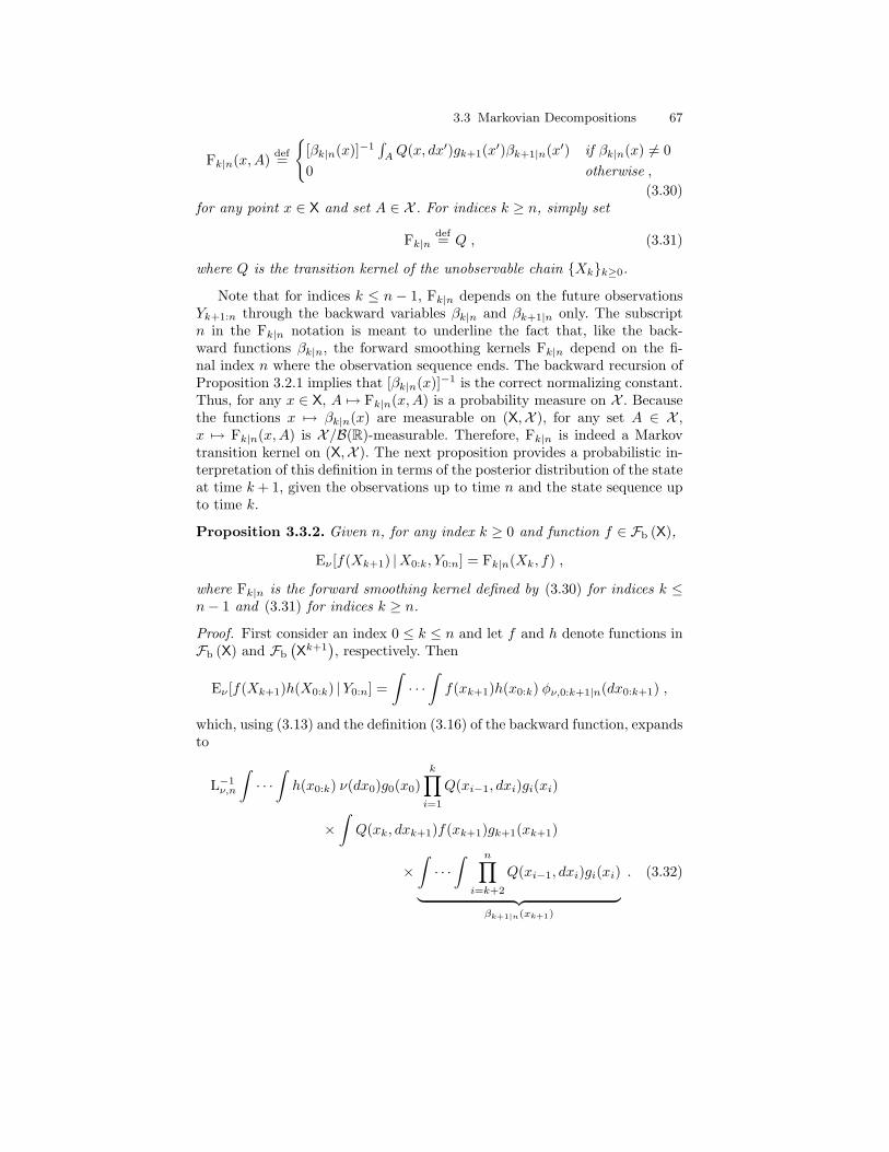
3.3 Markovian Decompositions 67

Fk|n(x,A) def=

[βk|n(x)]−1

∫AQ(x, dx′)gk+1(x′)βk+1|n(x′) if βk|n(x) 6= 0

0 otherwise ,(3.30)

for any point x ∈ X and set A ∈ X . For indices k ≥ n, simply set

Fk|ndef= Q , (3.31)

where Q is the transition kernel of the unobservable chain Xkk≥0.

Note that for indices k ≤ n − 1, Fk|n depends on the future observationsYk+1:n through the backward variables βk|n and βk+1|n only. The subscriptn in the Fk|n notation is meant to underline the fact that, like the back-ward functions βk|n, the forward smoothing kernels Fk|n depend on the fi-nal index n where the observation sequence ends. The backward recursion ofProposition 3.2.1 implies that [βk|n(x)]−1 is the correct normalizing constant.Thus, for any x ∈ X, A 7→ Fk|n(x,A) is a probability measure on X . Becausethe functions x 7→ βk|n(x) are measurable on (X,X ), for any set A ∈ X ,x 7→ Fk|n(x,A) is X/B(R)-measurable. Therefore, Fk|n is indeed a Markovtransition kernel on (X,X ). The next proposition provides a probabilistic in-terpretation of this definition in terms of the posterior distribution of the stateat time k + 1, given the observations up to time n and the state sequence upto time k.

Proposition 3.3.2. Given n, for any index k ≥ 0 and function f ∈ Fb (X),

Eν [f(Xk+1) |X0:k, Y0:n] = Fk|n(Xk, f) ,

where Fk|n is the forward smoothing kernel defined by (3.30) for indices k ≤n− 1 and (3.31) for indices k ≥ n.

Proof. First consider an index 0 ≤ k ≤ n and let f and h denote functions inFb (X) and Fb

(Xk+1

), respectively. Then

Eν [f(Xk+1)h(X0:k) |Y0:n] =∫· · ·∫f(xk+1)h(x0:k) φν,0:k+1|n(dx0:k+1) ,

which, using (3.13) and the definition (3.16) of the backward function, expandsto

L−1ν,n

∫· · ·∫h(x0:k) ν(dx0)g0(x0)

k∏i=1

Q(xi−1, dxi)gi(xi)

×∫Q(xk, dxk+1)f(xk+1)gk+1(xk+1)

×∫· · ·∫ n∏

i=k+2

Q(xi−1, dxi)gi(xi)︸ ︷︷ ︸βk+1|n(xk+1)

. (3.32)

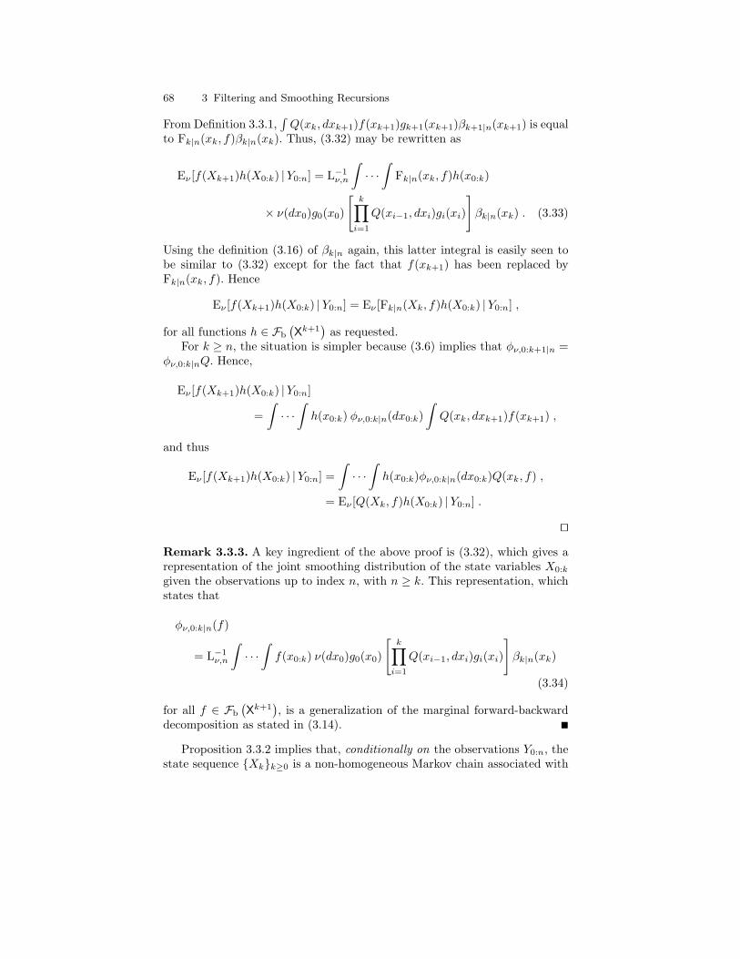
68 3 Filtering and Smoothing Recursions

From Definition 3.3.1,∫Q(xk, dxk+1)f(xk+1)gk+1(xk+1)βk+1|n(xk+1) is equal

to Fk|n(xk, f)βk|n(xk). Thus, (3.32) may be rewritten as

Eν [f(Xk+1)h(X0:k) |Y0:n] = L−1ν,n

∫· · ·∫

Fk|n(xk, f)h(x0:k)

× ν(dx0)g0(x0)

[k∏i=1

Q(xi−1, dxi)gi(xi)

]βk|n(xk) . (3.33)

Using the definition (3.16) of βk|n again, this latter integral is easily seen tobe similar to (3.32) except for the fact that f(xk+1) has been replaced byFk|n(xk, f). Hence

Eν [f(Xk+1)h(X0:k) |Y0:n] = Eν [Fk|n(Xk, f)h(X0:k) |Y0:n] ,

for all functions h ∈ Fb

(Xk+1

)as requested.

For k ≥ n, the situation is simpler because (3.6) implies that φν,0:k+1|n =φν,0:k|nQ. Hence,

Eν [f(Xk+1)h(X0:k) |Y0:n]

=∫· · ·∫h(x0:k) φν,0:k|n(dx0:k)

∫Q(xk, dxk+1)f(xk+1) ,

and thus

Eν [f(Xk+1)h(X0:k) |Y0:n] =∫· · ·∫h(x0:k)φν,0:k|n(dx0:k)Q(xk, f) ,

= Eν [Q(Xk, f)h(X0:k) |Y0:n] .

ut

Remark 3.3.3. A key ingredient of the above proof is (3.32), which gives arepresentation of the joint smoothing distribution of the state variables X0:k

given the observations up to index n, with n ≥ k. This representation, whichstates that

φν,0:k|n(f)

= L−1ν,n

∫· · ·∫f(x0:k) ν(dx0)g0(x0)

[k∏i=1

Q(xi−1, dxi)gi(xi)

]βk|n(xk)

(3.34)

for all f ∈ Fb

(Xk+1

), is a generalization of the marginal forward-backward

decomposition as stated in (3.14).

Proposition 3.3.2 implies that, conditionally on the observations Y0:n, thestate sequence Xkk≥0 is a non-homogeneous Markov chain associated with

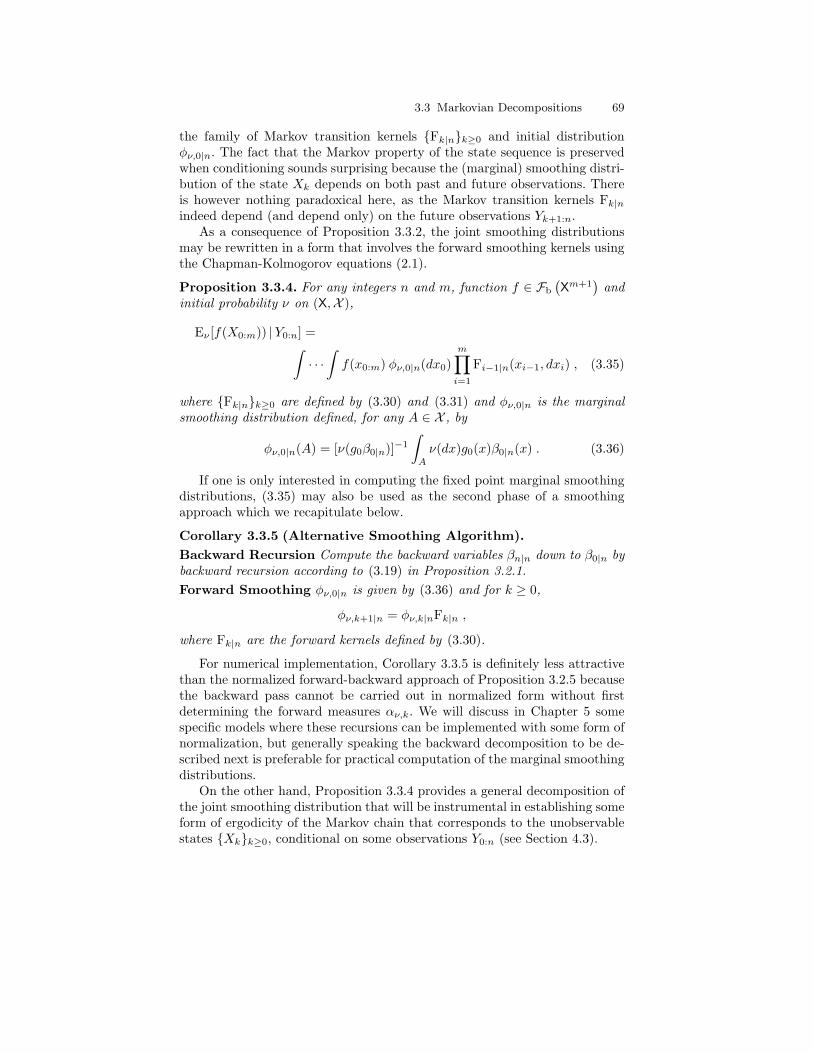
3.3 Markovian Decompositions 69

the family of Markov transition kernels Fk|nk≥0 and initial distributionφν,0|n. The fact that the Markov property of the state sequence is preservedwhen conditioning sounds surprising because the (marginal) smoothing distri-bution of the state Xk depends on both past and future observations. Thereis however nothing paradoxical here, as the Markov transition kernels Fk|nindeed depend (and depend only) on the future observations Yk+1:n.

As a consequence of Proposition 3.3.2, the joint smoothing distributionsmay be rewritten in a form that involves the forward smoothing kernels usingthe Chapman-Kolmogorov equations (2.1).

Proposition 3.3.4. For any integers n and m, function f ∈ Fb

(Xm+1

)and

initial probability ν on (X,X ),

Eν [f(X0:m)) |Y0:n] =∫· · ·∫f(x0:m) φν,0|n(dx0)

m∏i=1

Fi−1|n(xi−1, dxi) , (3.35)

where Fk|nk≥0 are defined by (3.30) and (3.31) and φν,0|n is the marginalsmoothing distribution defined, for any A ∈ X , by

φν,0|n(A) = [ν(g0β0|n)]−1

∫A

ν(dx)g0(x)β0|n(x) . (3.36)

If one is only interested in computing the fixed point marginal smoothingdistributions, (3.35) may also be used as the second phase of a smoothingapproach which we recapitulate below.

Corollary 3.3.5 (Alternative Smoothing Algorithm).Backward Recursion Compute the backward variables βn|n down to β0|n bybackward recursion according to (3.19) in Proposition 3.2.1.Forward Smoothing φν,0|n is given by (3.36) and for k ≥ 0,

φν,k+1|n = φν,k|nFk|n ,

where Fk|n are the forward kernels defined by (3.30).

For numerical implementation, Corollary 3.3.5 is definitely less attractivethan the normalized forward-backward approach of Proposition 3.2.5 becausethe backward pass cannot be carried out in normalized form without firstdetermining the forward measures αν,k. We will discuss in Chapter 5 somespecific models where these recursions can be implemented with some form ofnormalization, but generally speaking the backward decomposition to be de-scribed next is preferable for practical computation of the marginal smoothingdistributions.

On the other hand, Proposition 3.3.4 provides a general decomposition ofthe joint smoothing distribution that will be instrumental in establishing someform of ergodicity of the Markov chain that corresponds to the unobservablestates Xkk≥0, conditional on some observations Y0:n (see Section 4.3).

70 3 Filtering and Smoothing Recursions

3.3.2 Backward Decomposition

In the previous section it was shown that, conditionally on the observationsup to index n, Y0:n, the state sequence Xkk≥0 is a Markov chain, withtransition kernels Fk|n. We now turn to the so-called time-reversal issue: is ittrue in general that the unobserved chain with the indices in reverse order,forms a non-homogeneous Markov chain, conditionally on some observationsY0:n?

We already discussed time-reversal for Markov chains in Section 2.1 whereit has been argued that the main technical difficulty consists in guaranteeingthat the reverse kernel does exist. For this, we require somewhat strongerassumptions on the nature of X by assuming for the rest of this section that Xis a Polish space and that X is the associated Borel σ-field. From the discussionin Section 2.1 (see Definition 2.1.2 and comment below), we then know thatthe reverse kernel does exist although we may not be able to provide a simpleclosed-form expression for it. The reverse kernel does have a simple expression,however, as soon as one assumes that the kernel to be reversed and the initialdistribution admit densities with respect to some measure on X.

Let us now return to the smoothing problem. For positive indices k suchthat k ≤ n−1, the posterior distribution of (Xk, Xk+1) given the observationsup to time k satisfies

Eν [f(Xk, Xk+1) |Y0:k] =∫∫

f(xk, xk+1) φν,k(dxk)Q(xk, dxk+1) (3.37)

for all f ∈ Fb (X× X). From the previous discussion, there exists a Markovtransition kernel Bν,k which satisfies Definition 2.1.2, that is

Bν,kdef= Bν,k(x,A), x ∈ X, A ∈ X

such that for any function f ∈ Fb (X× X),

Eν [f(Xk, Xk+1) |Y0:k] =∫∫

f(xk, xk+1)φν,k+1|k(dxk+1) Bν,k(xk+1, dxk) ,

(3.38)where φν,k+1|k = φν,kQ is the one-step predictive distribution.

Proposition 3.3.6. Given a strictly positive index n, initial distribution ν,and index k ∈ 0, . . . , n− 1,

Eν [f(Xk) |Xk+1:n, Y0:n] = Bν,k(Xk+1, f)

for any f ∈ Fb (X). Here, Bν,k is the backward smoothing kernel definedin (3.38).

Before giving the proof of this result, we make a few remarks to providesome intuitive understanding of the backward smoothing kernels.

3.3 Markovian Decompositions 71

Remark 3.3.7. Contrary to the forward kernel, the backward transition ker-nel is only defined implicitly through the equality of the two representa-tions (3.37) and (3.38). This limitation is fundamentally due to the fact thatthe backward kernel implies a non-trivial time-reversal operation.

Proposition 3.3.6 however allows a simple interpretation of the back-ward kernel: Because Eν [f(Xk) |Xk+1:n, Y0:n] is equal to Bν,k(Xk+1, f) andthus depends neither on Xl for l > k + 1 nor on Yl for l ≥ k + 1, thetower property of conditional expectation (Proposition A.2.3) implies thatnot only is Bν,k(Xk+1, f) equal to Eν [f(Xk) |Xk+1, Y0:n] but also coincideswith Eν [f(Xk) |Xk+1, Y0:k], for any f ∈ Fb (X). In addition, the distributionof Xk+1 given Xk and Y0:k reduces to Q(Xk, ·) due to the particular formof the transition kernel associated with a hidden Markov model (see Defini-tion 2.2.1). Recall also that the distribution of Xk given Y0:k is denoted byφν,k. Thus, Bν,k can be interpreted as a Bayesian posterior in the equivalentpseudo-model where

• Xk is distributed a priori according to the filtering distribution φν,k,• The conditional distribution of Xk+1 given Xk is Q(Xk, ·).

Bν,k(Xk+1, ·) is then interpreted as the posterior distribution of Xk givenXk+1 in this equivalent pseudo-model.

In particular, for HMMs that are “fully dominated” in the sense of Def-inition 2.2.3, Q has a transition probability density function q with respectto a measure λ on X. This is then also the case for φν,k, which is a marginalof (3.13). In such cases, we shall use the slightly abusive but unambiguousnotation φν,k(dx) = φν,k(x)λ(dx) (that is, φν,k denotes the probability den-sity function with respect to λ rather than the probability distribution). Thebackward kernel Bν,k(xk+1, ·) then has a probability density function withrespect to λ, which is given by Bayes’ formula,

Bν,k(xk+1, x) =φν,k(x)q(x, xk+1)∫

Xφν,k(x)q(x, xk+1)λ(dx)

. (3.39)

Thus, in many cases of interest, the backward transition kernel Bν,k canbe written straightforwardly as a function of φν,k and Q. Several examples ofsuch cases will be dealt with in some detail in Chapter 5. In these situations,Proposition 3.3.9 is the method of choice for smoothing, as it only involvesnormalized quantities, whereas Corollary 3.3.5 is not normalized and thus cangenerally not be implemented as it stands.

Proof (of Proposition 3.3.6). Let k ∈ 0, . . . , n−1 and h ∈ Fb

(Xn−k

). Then

Eν [f(Xk)h(Xk+1:n) |Y0:n] =∫· · ·∫f(xk)h(xk+1:n) φν,k:n|n(dxk:n) . (3.40)

Using the definition (3.13) of the joint smoothing distribution φν,k:n|n yields

72 3 Filtering and Smoothing Recursions

Eν [f(Xk)h(Xk+1:n) |Y0:n]

= L−1ν,n

∫· · ·∫ν(dx0)g0(x0)

k∏i=1

Q(xi−1, dxi)gi(xi)f(xk)

×

[n∏

i=k+1

Q(xi−1, dxi)gi(xi)

]h(xk+1:n) ,

=Lν,kLν,n

∫∫φν,k|n(dxk)Q(xk, dxk+1)f(xk)gk+1(xk+1)

×∫· · ·∫ [ n∏

i=k+2

Q(xi−1, dxi)gi(xi)

]h(xk+1:n) , (3.41)

which implies, by the definition (3.38) of the backward kernel, that

Eν [f(Xk)h(Xk+1:n) |Y0:n]

=Lν,kLν,n

∫∫Bν,k(xk+1, dxk)f(xk)φν,k+1|k(dxk+1)gk+1(xk+1)

×∫· · ·∫ [ n∏

i=k+2

Q(xi−1, dxi)gi(xi)

]h(xk+1:n) . (3.42)

Taking f ≡ 1 shows that for any function h′ ∈ Fb

(Xn−k

),

Eν [h′(Xk+1:n) |Y0:n] =Lν,kLν,n

∫· · ·∫h′(xk+1:n)

× φν,k+1|k(dxk+1)gk+1(xk+1)n∏

i=k+2

Q(xi−1, dxi)gi(xi) .

Identifying h′ with h(xk+1:n)∫f(x) Bν,k(xk+1, dx), we find that (3.42) may

be rewritten as

Eν [f(Xk)h(Xk+1:n) |Y0:n]

= Eν

[h(Xk+1:n)

∫Bν,k(Xk+1, dx)f(x)

∣∣∣∣ Y0:n

],

which concludes the proof. ut

The next result is a straightforward consequence of Proposition 3.3.6,which reformulates the joint smoothing distribution φν,0:n|n in terms of thebackward smoothing kernels.

Corollary 3.3.8. For any integer n > 0 and initial probability ν,

Eν [f(X0:n) |Y0:n] =∫· · ·∫f(x0:m) φν,n(dxn)

n−1∏k=0

Bν,k(xk+1, dxk) (3.43)

3.3 Markovian Decompositions 73

for all f ∈ Fb

(Xn+1

). Here, Bν,k0≤k≤n−1 are the backward smoothing ker-

nels defined in (3.38) and φν,n is the marginal filtering distribution corre-sponding to the final index n.

It follows from Proposition 3.3.6 and Corollary 3.3.8 that, conditionally onY0:n, the joint distribution of the index-reversed sequence Xk0≤k≤n, withXk = Xn−k, is that of a non-homogeneous Markov chain with initial distri-bution φν,n and transition kernels Bν,n−k1≤k≤n. This is an exact analog ofthe forward decomposition where the ordering of indices has been reversed,starting from the end of the observation sequence and ending with the firstobservation. Three important differences versus the forward decompositionshould however be kept in mind.

(i) The backward smoothing kernel Bν,k depends on the initial distribu-tion ν and on the observations up to index k but it depends neitheron the future observations nor on the index n where the observationsequence ends. As a consequence, the sequence of backward transitionkernels Bν,k0≤k≤n−1 may be computed by forward recurrence on k, ir-respectively of the length of the observation sequence. In other terms, thebackward smoothing kernel Bν,k depends only on the filtering distribu-tion φν,k, whereas the forward smoothing kernel Fk|n was to be computedfrom the backward function βk|n.

(ii) Because Bν,k depends on φν,k rather than on the unnormalized forwardmeasure αν,k, its computation involves only properly normalized quanti-ties (Remark 3.3.7). The backward decomposition is thus more adaptedto the actual computation of the smoothing probabilities than the for-ward decomposition. The necessary steps are summarized in the followingresult.

Proposition 3.3.9 (Forward Filtering/Backward Smoothing).

Forward Filtering Compute, forward in time, the filtering distributions φν,0to φν,n using the recursion (3.22). At each index k, the backward transitionkernel Bν,k may be computed according to (3.38).Backward Smoothing From φν,n, compute, for k = n− 1, n− 2, . . . , 0,

φν,k|n = φν,k+1|n Bν,k ,

recalling that φν,n|ndef= φν,n.

(iii) A more subtle difference between the forward and backward Markoviandecompositions is the observation that Definition 3.3.1 does provide anexpression of the forward kernels Fk|n for any k ≥ 0, that is, also forindices after the end of the observation sequence. Hence, the processXkk≥0, when conditioned on some observations Y0:n, really forms anon-homogeneous Markov chain whose finite-dimensional distributionsare defined by Proposition 3.3.4. In contrast, the backward kernels Bν,k

74 3 Filtering and Smoothing Recursions

are defined for indices k ∈ 0, . . . , n−1 only, and thus the index-reversedprocess Xn−k is also defined, by Proposition 3.3.6, for indices k inthe range 0, . . . , n only. In order to define the index-reversed chainfor negative indices, a minimal requirement is that the underlying chainXk also be well defined for k < 0. Defining Markov chains Xk withindices k ∈ Z is only meaningful in the stationary case, that is when ν isthe stationary distribution of Q. As both this stationarization issue andthe forward and backward Markovian decompositions play a key rolein the analysis of the statistical properties of the maximum likelihoodestimator, we postpone further discussion of this point to Chapter 12.

3.4 Complements

The forward-backward algorithm is known to many, especially in the fieldof speech processing, as the Baum-Welch algorithm, although the first pub-lished description of the approach is due to Leonard E. Baum, Ted Petrie,George Soules, and Norman Weiss (1970, p. 168). The denomination refers tothe collaboration between Baum and Lloyd R. Welch (Welch, 2003) who alsoworked out together an early version of the EM approach (to be discussedin Chapter 10). To the best of our knowledge however, the note entitled “AStatistical Estimation Procedure for Probabilistic Functions of Finite MarkovProcesses”, co-authored by Baum and Welch and mentioned in the bibliogra-phy of Baum et al. (1970), has never been published.

The forward-backward algorithm was discovered several times in the early1970s. A salient example is the paper by Bahl et al. (1974) on the compu-tation of posterior probabilities for a finite-state Markov channel encoder fortransmission over a discrete memoryless channel (see Example 1.3.2 in theintroductory chapter). The algorithm described by Bahl et al. (1974) is fullyequivalent to the forward-backward and is known in digital communicationas the BCJR (for Bahl, Cocke, Jelinek, and Raviv) algorithm. Chang andHancock (1966) is another less well-known reference, contemporary of thework of Baum and his colleagues, which also describes the forward-backwarddecomposition and its use for decoding in communication applications.

It is important to keep in mind that the early work on HMMs by Baumand his colleagues was conducted at the Institute for Defense Analyses (IDA)in Princeton under a contract from the U.S. National Security Agency. Al-though there are a few early publications of theoretical nature, most of thepractical work that dealt with cryptography was kept secret and has neverbeen published. It explains why some significant practical aspects (like theneed for scaling to be discussed below) remained unpublished until HMMsbecame the de facto standard approach to speech recognition in the 1980s.

The famous tutorial by Rabiner (1989) is considered by many as the stan-dard source of information for practical implementation of hidden Markov

3.4 Complements 75

models. The impact of this publication has been very significant in speech pro-cessing but also in several other domains of application such as bioinformat-ics (Durbin et al., 1998). It was Rabiner (1989) who coined the term scaling todescribe the need for normalization when implementing the forward-backwardrecursions. There is indeed a subtle difference between the normalizationscheme described in Section 3.2.2 and the solution advocated by Rabiner(1989), which was first published by Levinson et al. (1983). As was done inSection 3.2.2, Rabiner (1989) recommends normalizing the forward measuresso that they integrate to one. However, the normalized backward functions aredefined as βk|n = (

∏nl=k cν,l)

−1βk|n rather than βn|n = (∏nl=k+1 cν,l)

−1βk|n.This difference is a consequence of the normalized backward recursion beingcarried out as

βn|n(x) = c−1ν,n and

βk|n(x) = c−1ν,k

∫X

Q(x, dx′)gk+1(x′)βk+1|n(x′) for k = n− 1 down to 0,

rather than as prescribed by (3.23). In contrast to our approach, Rabiner’sscaling implies that normalization is still required for computing the marginalsmoothing distributions as

φν,k|n(dx) = [φν,k(βk|n)]−1βk|n(x)φν,k(dx) .

On the other hand, the joint smoothing distribution φν,k:k+1|n of Xk and Xk+1

may be obtained directly, without normalization, as

φν,k:k+1|n(dx, dx′) = φν,k(dx)Q(x, dx′)gk+1(x′)βk+1|n(x′) .

Indeed, φν,k = (∏kl=0 cν,l)

−1αν,k and thus

φν,k:k+1|n(dx, dx′) =

(n∏l=0

cν,l

)−1

αν,k(dx)Q(x, dx′)gk+1(x′)βk+1|n(x′) ,

as requested, as Lν,n =∏nl=0 cν,l is the normalization factor common to all

smoothing distributions from (3.13).Easy computation of bivariate smoothing distributions does not, in our

view, constitute a strong motivation for preferring a particular scaling scheme.The Markovian structure of the joint smoothing distribution exhibited in Sec-tion 3.3 in particular provides an easy means of evaluating bivariate smoothingdistributions. For instance, with the scaling scheme described in Section 3.2.2,the forward Markovian decomposition of Section 3.3.1 implies that

φν,k:k+1|n(dx, dx′) = cν,kφν,k|n(dx)Q(x, dx′)gk+1(x′)βk+1|n(x′)

βk|n(x).

As stated in the introduction, Stratonovich (1960) proposed a decomposi-tion that is largely related to the forward-backward approach when the state

76 3 Filtering and Smoothing Recursions

space X is discrete. The forward measure, named w in the work of Stratonovich(1960), is defined as

wk(x) = Pν(Xk = x |Y0:k) ,

which coincides with the definition of the filtering probability φν,k for a dis-crete X. Also recall that φν,k corresponds to the normalized forward variableαν,k = [αν,k(1)]−1αν,k. Instead of the backward function, Stratonovich (1960)defined

wk(x) = Pν(Xk = x |Yk:n) .

Forward and backward recursions for wk and wk, respectively, as well as therelation for computing the marginal smoothing probability from wk and wk,are given in the first section of Stratonovich (1960) on pages 160–162. Al-though wk as defined by Stratonovich (1960) obviously has a probabilisticinterpretation that the backward function lacks, the resulting recursion ismore complicated because it requires the evaluation of the prior probabilitiesPν(Xk = x) for k ≥ 0. In addition, generalizing the definition of wk to gen-eral state spaces X would require using the more restrictive index- (or time-)reversal concept discussed in Section 3.3.2. In contrast, the forward-backwarddecomposition of Baum et al. (1970) provides a very general framework forsmoothing as discussed in this chapter.

The fact that, in some cases, a probabilistic interpretation may be given tothe backward function βk|n (or to equivalent quantities) also explains why inthe control and signal processing literatures, the forward-backward recursionsare known under the generic term of two-filter formulas (Kitagawa, 1996;Kailath et al., 2000, Section 10.4). This issue will be discussed in detail forGaussian linear state-space models in Section 5.2.5.

4

Advanced Topics in Smoothing

This chapter covers three distinct complements to the basic smoothing rela-tions developed in the previous chapter.

In the first section, we provide recursive smoothing relations for computingsmoothed expectations of general functions of the hidden states. In manyrespects, this technique is reminiscent of the filtering recursion detailed inSection 3.2.2, but somewhat harder to grasp because the quantity that needsto be updated recursively is less directly interpretable.

In the second section, it is shown that the filtering and smoothing ap-proaches discussed so far (including those of Section 4.1) may be applied,with minimal adaptations, to a family of models that is much broader thansimply the hidden Markov models. We consider in some detail the case ofhierarchical HMMs (introduced in Section 1.3.4) for which marginal filteringand smoothing formulas are still available, despite the fact that the hierarchiccomponent of the state process is not a posteriori Markovian.

The third section is different in nature and is devoted to the so-calledforgetting property of the filtering and smoothing recursions, which are in-strumental in the statistical theory of HMMs (see Chapter 12). Forgettingrefers to the fact that observations that are either far back in the past orin the remote future (relative to the current time index) have little impacton the posterior distribution of the current state. Although this section iswritten to be self-contained, its content is probably better understood aftersome exposure to the stability properties of Markov chains as can be found inChapter 14.

4.1 Recursive Computation of Smoothed Functionals

Chapter 3 mostly dealt with fixed-interval smoothing, that is, computationof φk|n1 for a fixed value of the observation horizon n and for all indices

1Note that we omit the dependence with respect to the initial distribution ν,which is not important in this section.

78 4 Advanced Topics in Smoothing

0 ≤ k ≤ n. For Gaussian linear state-space models, it is well-known howeverthat recursive (in n) evaluation of φk|n for a fixed value of k, also calledfixed-point smoothing, is feasible (Anderson and Moore, 1979, Chapter 7).Gaussian linear state-space models certainly constitute a particular case, asthe smoothing distributions φk|n are then entirely defined by their first andsecond moments (see Chapter 5). But fixed-point smoothing is by no meanslimited to some specific HMMs and (3.13) implies the existence of recursiveupdate equations for evaluating φk|n with k fixed and increasing values of n.Remember that, as was the case in the previous chapter, we consider for themoment that evaluating integrals on X is a feasible operation.

The good news is that there also exist recursive formulas for computinga large class of smoothed quantities, which include in particular expressionslike E[

∑nk=0 s(Xn) |Y0:n] and E[(

∑nk=0 s(Xn))2 |Y0:n], where s is a real-valued

measurable function on (X,X ) such that both expectations are well-defined.Although one can of course consider arbitrary functions in this class, we willsee in Chapter 10 that smoothed expectations of the state variables, for somespecific choices of the function of interest, are instrumental in numerical ap-proximations of the maximum likelihood estimate for parameter-dependentHMMs.

4.1.1 Fixed Point Smoothing

The fundamental equation here is (3.13), which upon comparing the expres-sions corresponding to n and n+1 gives the following update equation for thejoint smoothing distribution:

φ0:n+1|n+1(fn+1) =(

Ln+1

Ln

)−1 ∫· · ·∫fn+1(x0:n+1)

φ0:n|n(dx0, . . . , dxn)Q(xn, dxn+1) gn+1(xn+1) (4.1)

for functions fn+1 ∈ Fb

(Xn+2

). Recall that we used the notation cn+1 for the

scaling factor Ln+1/Ln that appears in (4.1), where, according to (3.27), cn+1

may also be evaluated as φn+1|n(gn+1).Equation (4.1) corresponds to a simple, yet rich, structure in which the

joint smoothing distribution is modified by applying an operator that onlyaffects the last coordinate2. The probabilistic interpretation of this finding isthat Xn+1 and X0:n−1 are conditionally independent given both Y0:n+1 andXn. This remark suggests that while the objective of updating φk|n recur-sively in n (for a fixed k) may not be achievable directly, φk,n|n—the jointdistribution of Xk and Xn given Y0:n—does follow a simple recursion.

Proposition 4.1.1 (Fixed Point Smoothing). For k ≥ 0 and any f ∈Fb

(X2),

2This structure also has deep implications, which we do not comment on here,for sequential Monte Carlo approaches (to be discussed in Chapters 7 and 8).

4.1 Recursive Computation of Smoothed Functionals 79

φk,k+1|k+1(f) = c−1k+1

∫∫f(xk, xk+1)φk(dxk)Q(xk, dxk+1) gk+1(xk+1) ,

where φk is the filtering distribution and ck+1 = φkQgk+1. For n ≥ k+ 1 andany f ∈ Fb

(X2),

φk,n+1|n+1(f) =

c−1n+1

∫∫f(xk, xn+1)

∫φk,n|n(dxk, dxn)Q(xn, dxn+1) gn+1(xn+1) .

Both relations are obtained by integrating (4.1) over all variables but those ofrelevant indices (k and k + 1 for the first one, k, n, and n+ 1 for the secondone). At any index n, the marginal smoothing distribution may be evalu-ated through φk|n = φk,n|n(·,X). Similarly the filtering distribution, which isrequired to evaluate cn+1, is given by φn = φk,n|n(X, ·).

4.1.2 Recursive Smoothers for General Functionals

From Proposition 4.1.1, one can easily infer a smoothing scheme that appliesto the specific situation where the only quantity of interest is E[s(Xk) |Y0:n]for a particular function s, and not the full conditional distribution φk,n|n. Tothis aim, define the finite signed measure τn on (X,X ) by

τn(f) =∫f(xn) s(xk)φk,n|n(dxk, dxn) , f ∈ Fb (X) ,

so that τn(X) = E[s(Xk) |Y0:n]. Proposition 4.1.1 then implies that

τk+1(f) = c−1k+1

∫f(xk+1)

∫s(xk)φk(dxk)Q(xk, dxk+1) gk+1(xk+1) ,

and

τn+1(f) = c−1n+1

∫f(xn+1)

∫τn(dxn)Q(xn, dxn+1) gn+1(xn+1) (4.2)

for n ≥ k + 1 and f ∈ Fb (X). Equation (4.2) is certainly less informativethan Proposition 4.1.1, as one needs to fix the function s whose smoothedconditional expectation is to be updated recursively. On the other hand, thisprinciple may be adapted to compute smoothed conditional expectations fora general class of functions that depend on the whole trajectory of the hiddenstates X0:n rather than on just a single particular hidden state Xk.

Before exposing the general framework, we first need to clarify a matter ofterminology. In the literature on continuous time processes, and particularlyin works that originate from the automatic control community, it is fairlycommon to refer to quantities similar to τn as filters—see for instance Elliottet al. (1995, Chapters 5 and 6) or Zeitouni and Dembo (1988). A filter is then

80 4 Advanced Topics in Smoothing

defined as an object that may be evaluated recursively in n and is helpful incomputing a quantity of interest that involves the observations up to indexn. A more formal definition, which will also illustrate what is the precisemeaning of the word recursive, is that a filter τnn≥0 is such that τ0 =Rν(Y0) and τn+1 = Rn(τn, Yn+1) where Rν and Rnn≥0 are some non-random operators. In the case discussed at the beginning of this section, Rn

is defined by (4.2) where Q is fixed (this is the transition kernel of the hiddenchain) and Yn+1 enters through gn+1(x) = g(x, Yn+1). Note that because thenormalizing constant c−1

n+1 in (4.2) depends on φn, Q and gn+1, to be coherentwith our definition we should say that φn, τnn≥0 jointly forms a filter. In thisbook, we however prefer to reserve the use of the word filter to designate thestate filter φn. We shall refer to quantities similar to τnn≥0 as the recursivesmoother associated with the functional tnn≥0, where the previous examplecorresponds to tn(x0, . . . , xn) = s(xk). It is not generally possible to derive arecursive smoother without being more explicit about the family of functionstnn≥0. The device that we will use in the following consists in specifyingtnn≥0 using a recursive formula that involves a set of fixed-dimensionalfunctions.

Definition 4.1.2 (Smoothing Functional). A smoothing functional is asequence tnn≥0 of functions such that tn is a function Xn+1 → R, and whichmay be defined recursively by

tn+1(x0:n+1) = mn(xn, xn+1)tn(x0:n) + sn(xn, xn+1) (4.3)

for all x0:n+1 ∈ Xn+2 and n ≥ 0, where mnn≥0 and snn≥0 are two se-quences of measurable functions X× X→ R and t0 is a function X→ R.

This definition can be extended to cases in which the functions tn are d-dimensional vector-valued functions. In that case, snn≥0 also are vector-valued functions X × X → Rd while mnn≥0 are matrix-valued functionsX× X→ Rd × Rd.

In simpler terms, a smoothing functional is such that the value of tn+1

in x0:n+1 differs from that of tn, applied to the sub-vector x0:n, only by amultiplicative and an additive factor that both only depend on the last twocomponents xn and xn+1. The whole family is thus entirely specified by t0and the two sequences mnn≥0 and snn≥0. This form has of course beenchosen because it reflects the structure observed in (4.1) for the joint smooth-ing distributions. It does however encompass some important functionals ofinterest. The first and most obvious example is when tn is a homogeneousadditive functional, that is, when

tn(x0:n) =n∑k=0

s(xk)

for a given measurable function s. In that case, sn(x, x′) reduces to s(x′) andmn is the constant function equal to 1.

4.1 Recursive Computation of Smoothed Functionals 81

The same strategy also applies for more complicated functions such as thesquared sum (

∑nk=0 s(xk))2. This time, we need to define two functions

tn,1(x0:n) =n∑k=0

s(xk) ,

tn,2(x0:n) =

[n∑k=0

s(xk)

]2

, (4.4)

for which we have the joint update formula

tn+1,1(x0:n+1) = tn,1(x0:n) + s(xn+1) ,

tn+1,2(x0:n+1) = tn,2(x0:n) + s2(xn+1) + 2s(xn+1)tn,1(x0:n) .

Note that these equations can also be considered as an extension of Defini-tion 4.1.2 for the vector valued function tn = (tn,1, tn,2)t.

We now wish to compute E[tn(X0:n) |Y0:n] recursively in n, assuming thatthe functions tn are such that these expectations are indeed finite. We proceedas previously and define the family of finite signed measures τn on (X,X )such that

τn(f) def=∫· · ·∫f(xn) tn(x0:n)φ0:n|n(dx0, . . . , dxn) (4.5)

for all functions f ∈ Fb (X). Thus, τn(X) = E[tn(X0:n) |Y0:n]. We then havethe following direct consequence of (4.1).

Proposition 4.1.3. Let (tn)n≥0 be a sequence of functions on Xn+1 → R pos-sessing the structure of Definition 4.1.2. The finite signed measures τnn≥0

on (X,X ) defined by (4.5) may then be updated recursively according to

τ0(f) = ν(g0)−1∫f(x0) ν(dx0) t0(x0) g0(x0)

and

τn+1(f) = c−1n+1

∫∫f(xn+1)

[τn(dxn)Q(xn, dxn+1) gn+1(xn+1)mn(xn, xn+1)

+φn(dxn)Q(xn, dxn+1) gn+1(xn+1)sn(xn, xn+1)]

(4.6)

for n ≥ 0, where f denotes a generic function in Fb (X). At any index n,E[tn(X0:n) |Y0:n] may be evaluated by computing τn(X).

In order to use (4.6), it is required that the standard filtering recursions(Proposition 3.2.5) be computed in parallel to (4.6). In particular, the nor-malizing constant cn+1 is given by (3.22) as

cn+1 = φnQgn+1 .

82 4 Advanced Topics in Smoothing

As was the case for Definition 4.1.2, Proposition 4.1.3 can obviously beextended to cases where the functional (tn)n≥0 is vector-valued, without anyadditional difficulty. Because the general form of the recursion defined byProposition 4.1.3 is quite complex, we first examine the simple case of homo-geneous additive functionals mentioned above.

Example 4.1.4 (First and Second Moment Functionals). Let s be afixed function on X and assume that the functionals of interest are the sumand squared sum in (4.4). A typical example is when the base function s equals1A for a some measurable set A. Then, E[tn,1(X0:n) |Y0:n] is the conditionalexpected occupancy of the set A by the hidden chain Xkk≥0 between indices0 and n. Likewise, E[tn,2(X0:n) |Y0:n]−(E[tn,1(X0:n) |Y0:n])2 is the conditionalvariance of the occupancy of the set A.

We define the signed measures τn,1 and τn,2 associated to tn,1 and tn,2by (4.5). We now apply the general formula given by Proposition 4.1.3 toobtain a recursive update for τn,1 and τn,2:

τ0,1(f) = [ν(g0)]−1

∫f(x0) ν(dx0) s(x0)g0(x0) ,

τ0,2(f) = [ν(g0)]−1

∫f(x0) ν(dx0) s2(x0)g0(x0)

and, for n ≥ 0,

τn+1,1(f) =∫f(xn+1)[

φn+1(dxn+1) s(xn+1) + c−1n+1

∫τn,1(dxn)Q(xn, dxn+1) gn+1(xn+1)

],

τn+1,2(f) =∫f(xn+1)[

φn+1(dxn+1) s2(xn+1) + c−1n+1

∫τn,2(dxn)Q(xn, dxn+1) gn+1(xn+1)

+ 2c−1n+1

∫τn,1(dxn)Q(xn, dxn+1) gn+1(xn+1)s(xn+1)

].

4.1.3 Comparison with Forward-Backward Smoothing

It is important to contrast the approach of Section 4.1.2 above with the tech-niques discussed previously in Chapter 3. What are exactly the differencesbetween the recursive smoother of Proposition 4.1.3 and the various versionsof forward-backward smoothing discussed in Sections 3.2 and 3.3? Is it alwayspossible to apply either of the two approaches? If yes, is one of them preferable

4.1 Recursive Computation of Smoothed Functionals 83

to the other? These are important issues that we review below. Note that forthe moment we only compare these two approaches on principle grounds andwe do not even try to discuss the computational burden associated with theeffective implementation of either approach. This latter aspect is of courseentirely dependent of the way in which we are to evaluate (or approximate)integrals, which is itself highly dependent on the specific model under consid-eration. Several concrete applications of this approach will be considered inChapters 10 and 11.

4.1.3.1 Recursive Smoothing Is More General

Remember that in Chapter 3 our primary objective was to develop approachesfor computing marginal smoothing distributions φk|n = P(Xk ∈ · |Y0:n). Acloser inspection of the results indicate that both in the standard forward-backward approach (Section 3.2) or when using a Markovian (forward or back-ward) decomposition (Section 3.3), one may easily obtain the bivariate jointsmoothing distribution φk+1:k|n = P((Xk+1, Xk) ∈ · |Y0:n) as a by-product ofevaluating φk|n, with essentially no additional calculation (see in particularSection 3.4).

If we consider however the second-order functional tn,2 discussed in Ex-ample 4.1.4, we may write

E[tn,2(X0:n) |Y0:n] =n∑i=0

n∑j=0

E[s(Xi)s(Xj) |Y0:n] .

The conditional expectations on the right-hand side indeed only involve thebivariate joint smoothing distributions but for indices that are not consecu-tive: it is not sufficient to determine φk+1:k|n for k = 0, . . . , n− 1 to evaluateE[tn,2(X0:n) |Y0:n] directly. One would require the complete set of distribu-tions P[(Xi, Xj) ∈ · |Y0:n] for 0 ≤ i ≤ j ≤ n.

From this example we may conclude that computing E[tn(X0:n) |Y0:n] us-ing forward-backward smoothing is not possible for the whole class of func-tionals defined in (4.3) but only for a subset of it. If we are to use only thebivariate joint smoothing distributions φk+1:k|n, then tn must be an additivefunctional for which the multipliers mn are constant (say, equal to 1). In thatcase, tn reduces to

tn(x0:n) = t0(x0) +n−1∑k=0

sk(xk, xk+1) ,

and the expected value of tn may be directly evaluated as

E[tn(X0:n) |Y0:n] =∫t0(x0)φ0|n(dx0) +

n−1∑k=0

∫sk(xk, xk+1)φk:k+1|n(dxk, dxk+1) . (4.7)

84 4 Advanced Topics in Smoothing

Recursive smoothing is more general in the sense that it is not restricted tosum functionals but applies to the whole class of functions whose structureagrees with (4.3).

4.1.3.2 For Additive Functionals, Forward-Backward Is MoreGeneral

A distinctive feature however of recursive smoothing is that it may only beapplied once a particular function in the class has been selected. The recursivesmoother τn is associated with a specific choice of the functional tn. As anexample, denote by τn,A the recursive smoother associated with the homoge-neous sum functional

tn,A(x0:n) =n∑k=0

1A(xk)

for a given set A. We may compute τn,A, recursively in n using Proposi-tion 4.1.3 and evaluate

∑nk=0 P(Xk ∈ A |Y0:n) as τn,A(X). If we now consider

a different set B, there is no way of evaluating∑nk=0 P(Xk ∈ B |Y0:n) from the

previous recursive smoother τn,A. It is thus required to run a specific recursivesmoother for each function that we are possibly interested in.

In contrast, once we have evaluated φk+1:k|n for all indices k between 0and n−1, we may apply (4.7) to obtain the expectation of any particular sumfunctional that we might be interested in.

4.1.3.3 Recursive Smoothing Is Recursive!

A final element of the comparison of the two approaches is the fact thatforward-backward is fundamentally intended for a fixed amount of observa-tions, a situation usually referred to as block or batch processing. Consideragain, as an example, a simple sum functional of the form

tn(x0:n) =n∑k=0

s(xk) ,

and suppose that we are given our n observations not as a whole but one byone, starting with X0 and then X1, X2, etc.

If we use the normalized forward-backward recursions (Proposition 3.2.5)or the equivalent backward Markovian decomposition (Proposition 3.3.9), theonly quantities that are available at an intermediate index k (with k lessthan n) are the filtering distributions φ0 to φk. Although we could evaluateE[s(Xj) |Y0:j ] for j ≤ k, it is not yet possible to evaluate E[tk(X0:k) |Y0:k]. Tobe able to compute smoothed quantities, one must decide on an endpoint, sayk = n, from which the backward recursion is started. The backward recursionthen provides us with the smoothed marginal distributions φk|n from whichE[tk(X0:n) |Y0:n] can be evaluated. This is even more obvious for the forward

4.2 Filtering and Smoothing in More General Models 85

Markovian decomposition (Corollary 3.3.5), which starts by the backwardrecursion initialized at the final index n.

In contrast, for the recursive smoother, the update equation (4.6) in Propo-sition 4.1.3 provides a means of computing E[tk(X0:k) |Y0:k] for all indicesk = 1, 2, . . . , whether or not we have reached the final observation index.There need not even be a final observation index, and the method can beapplied also when n = ∞ or when the final observation index is not speci-fied. Note that in cases where n is finite but quite large, forward-backward(or the equivalent Markovian decompositions) requires that all the interme-diate results be stored: before we can compute φk|n we first need to evaluateand keep track of all the filtering distributions φ0 to φn (or, for the forwardMarkovian decomposition, the backward functions βn|n down to β0|n). Thusfor large values of n, recursive smoothing approaches are also preferable tothose based on forward-backward ideas.

Remember however that the price to pay for deriving a recursive smootheris the need to particularize the function of interest. We will discuss in Chap-ter 10 the exact computational cost of both approaches in examples of HMMsfor which the computation corresponding to Proposition 4.1.3 is actually fea-sible.

4.1.3.4 Bibliographic Notes

The recursive smoothing approach discussed in this section was first describedby Zeitouni and Dembo (1988) and Elliott (1993) for continuous time discretestate Markov processes observed in (Gaussian) noise. The approach is alsoat the core of the book by Elliott et al. (1995). The application of the sameprinciple to the specific case of Gaussian linear state-space models is consid-ered, among others, by Elliott and Krishnamurthy (1999) (see also referencestherein). The common theme of these works is to use the EM algorithm (seeChapter 10), replacing forward-backward smoothing by recursive smoothing.For reasons to be explained in Section 10.2, the functionals of interest in thiscontext are sums (that is, mn = 1 in Definition 4.1.2). We will see in Sec-tion 10.2.4 that the same approach (always with sum functionals) also appliesfor computing the gradient of the log-likelihood with respect to the parametersin parameterized models. The fact that the same approach applies for moregeneral functionals such as squared sums is, to the best of our knowledge, new(see also Section 10.3.4 for an example of this latter case).

4.2 Filtering and Smoothing in More General Models

Although our main interest is hidden Markov models as defined in Section 2.2,the smoothing decompositions and recursions derived so far turn out to be farmore general. We briefly discuss below the case of several non-HMM modelsof practical interest before considering the specific case of hierarchical HMMsas defined in Section 2.2.3.

86 4 Advanced Topics in Smoothing

4.2.1 Smoothing in Markov-switching Models

In Markov-switching models (see Section 1.3.6), the distribution of Yk givenX0:k and Y0:k−1 does not only depend on Xk but also on a number of past val-ues of the observed sequence. Assume for ease of notation that the dependencewith respect to previous observations is only on the last observation Yk−1. Itis easily checked that (3.1), which defines the joint distribution of a numberof consecutive hidden states and observations, should then be replaced by

Eν [f(X0, Y0, . . . , Xn, Yn)] =∫· · ·∫f(x0, y0, . . . , xn, yn)

× ν(dx0)h(x0, y0)n∏k=1

Q(xk−1, dxk) g [(xk, yk−1), yk] µn(dy0, . . . , dyn)

(4.8)

for all f ∈ Fb

(X× Yn+1

), where g[(xk, yk−1), ·] is the transition density

function of Yk given Xk and Yk−1. Note that for Markov-switching models,it is more natural to define the initial distribution as the joint distribution ofX0 and Y0 and hence as a probability measure on (X×Y,X ⊗Y). In (4.8), wehave adopted a particular and equivalent way of representing this distributionas ν(dx0)h(x0, dy0)µ(dy0) for some transition density function h.

Equation (4.8) is similar to (3.1) and will be even more so once we adoptthe implicit conditioning convention introduced in Section 3.1.4. Indeed, upondefining

g0(·) def= h(·, Y0) ,

gk(·) def= g [(·, Yk−1), Yk] for k ≥ 1 ,

the joint distribution φν,0:n|n of the hidden states X0:n given the observationsY0:n is still given by (3.13), and hence the mechanics of smoothing for switchingautoregressive models are the same as for the standard HMM (see for instanceHamilton, 1994, Chapter 22).

4.2.2 Smoothing in Partially Observed Markov Chains

It should also be clear that the same remark holds, mutatis mutandis, for othervariants of the model such as non-homogeneous ones—if Q depends on theindex k for instance—or if the transition from Xk to Xk+1 also depends onsome function of the past observations Y0:k−1. Moreover, a closer inspectionof the smoothing relations obtained previously indicate that, except when onewishes to exhibit predicted quantities—as in (3.27)—only the unnormalizedproduct kernel Rk−1(xk−1, dxk) = Q(xk−1, dxk) gk(xk) does play a role3. In

3We will come back to this remark when examining sequential Monte Carloapproaches in Chapter 7.

4.2 Filtering and Smoothing in More General Models 87

particular, for the general class of models in which it is only assumed thatXk, Ykk≥0 jointly form a Markov chain, the joint distribution of Yk and Xk

given Yk−1 and Xk−1 may be represented as

Q [(xk−1, yk−1), dxk] g [(xk−1, yk−1, xk), yk]µ(dyk) ,

assuming that the second conditional distribution is dominated by µ. Hencein this case also, one may define

Rk−1(xk−1, dxk) def= Q [(xk−1, Yk−1), dxk] g [(xk−1, Yk−1, xk), Yk]

and use the same filtering and smoothing relations as before. With this nota-tion, it is a simple matter of rewriting, replacing the product of Q and gk byRk−1 to obtain, for instance, the filtering update from (3.22):

cν,k =∫∫

φν,k−1(dx)Rk−1(x, dx′) ,

φν,k(f) = c−1ν,k

∫f(x′)

∫φν,k−1(dx)Rk−1(x, dx′) , f ∈ Fb (X) .

4.2.3 Marginal Smoothing in Hierarchical HMMs

An example that nicely illustrates the previous discussion on the generality ofthe filtering and smoothing recursions of Chapter 3 is the case of hierarchicalHMMs. These models defined in Section 2.2.3 are hidden Markov models inwhich the unobservable chain Xkk≥0 is split into two components Ckk≥0

and Wkk≥0 such that the component Ckk≥0, which is the highest in the hi-erarchy, marginally forms a Markov chain. Of course, these models are HMMsand can be handled as such. In many cases, it is however advantageous toconsider that the component of interest is Ckk≥0 only, marginalizing withrespect to the intermediate component Wkk≥0. A typical example is the caseof conditionally Gaussian linear state-space models (Definition 2.2.6), wherethe indicator component Ck takes values in a finite set, whereas the intermedi-ate component Wk is a vector-valued, possibly high-dimensional, variable. It isclear however that the pair (Ck, Yk) does not correspond to a hidden Markovmodel. In particular, the distribution of Yn depends on all indicator variablesC0 up to Cn (rather than on Cn only), due to the marginalization of the inter-mediate variables W0:n. Because of the generality of the smoothing relationsobtained in Chapter 3, the implementation of marginal smoothing—that is,estimation of Ckk≥0 only given Ykk≥0—however bears some similaritywith the (simpler) case of HMMs.

For notational simplicity, we consider in the remainder of this section thatthe hierarchic component Ckk≥0 takes values in the finite set 1, . . . , r.As usual in this context, we use the notations QC(x, x′) and νC(x) ratherthan QC(x, x′) and νC(x). The other notations pertaining to hierarchical

88 4 Advanced Topics in Smoothing

hidden Markov models can be found in Section 2.2.3. Let ψν,0:k|k denote theposterior distribution of C0:k given Y0:k,

ψν,0:k|k(c0:k) def= Pν (C0:k = c0:k |Y0:k) . (4.9)

Using (3.13) for the hierarchical HMM and integrating with respect to theintermediate component w0:n readily gives

ψν,0:n|n (c0:n) = L−1ν,n νC(c0)

n∏k=1

QC(ck−1, ck)

∫· · ·∫νW (c0, dw0)

n∏k=1

QW [(wk−1, ck), dwk] gk(ck, wk) , (4.10)

where gk(ck, wk) def= g [(ck, wk), Yk]. Comparing the above expression for twosuccessive indices, say n and n+ 1, yields

ψν,0:n+1|n+1 (c0:n+1) =(

Lν,n+1

Lν,n

)−1

ψν,0:n|n (c0:n)QC(cn, cn+1)∫ϕν,n+1|n(c0:n+1, dwn+1) gn+1(cn+1, wn+1) , (4.11)

where

ϕν,n+1|n(c0:n+1, f) def=∫Wn+1

νW (c0, dw0)

n∏k=1

QW [(wk−1, ck), dwk]gk(ck, wk)QW [(wn, cn+1), f ]

∫Wn+1

νW (c0, dw0)n∏k=1

QW [(wk−1, ck), dwk]gk(ck, wk)

(4.12)

for f ∈ Fb (W), which is recognized as the predictive distribution of theintermediate component Wn+1 given the observations Y0:n up to index n andthe indicator variables C0:n+1 up to index n+ 1.

In the example of conditionally Gaussian linear state-space models, theconditional predictive distribution ϕν,n+1|n(c0:n+1, ·) given in (4.12) is Gaus-sian and may indeed be evaluated recursively for a given sequence of indicatorvariables c0:n+1 using the Kalman recursions (see Section 5.2). Moreover, inthese models the integral featured on the second line of (4.11) may also beevaluated exactly. It is important however to understand that even in this(favorable) case, the existence of (4.11) does not provide an easy solution toupdating the marginal filtering distribution ψν,n|n as it does for HMMs. Thefundamental problem is that (4.12) also directly indicates that the predictivedistribution Wn+1 given Y0:n, but without conditioning on the indicator vari-ables C0:n+1, is a mixture distribution with a number of components equal

4.3 Forgetting of the Initial Condition 89

to the number of possible configurations of C0:n+1, that is, rn+2. Hence inpractice, even in cases such as the conditionally Gaussian linear state-spacemodels for which evaluation of (4.12) is feasible, it is not possible to imple-ment the exact marginal filtering relations for the sequence Ckk≥0 becauseof the combinatorial explosion due to the need to enumerate all configurationsof the indicator variables.

Thus, (4.1) will only be helpful in approaches where it is possible to imputevalues to (part of) the unknown sequence Ckk≥0, making it possible toavoid exhaustive enumeration of all configurations of the indicator variables.This is precisely the aim of sequential Monte Carlo methods to be describedin Chapters 7 and 8, where the specific case of hierarchical HMMs will bedetailed in Section 8.2.

Note that while (4.1) obviously suggests a recursion in increasing values ofn, it is also possible to write an analog to the forward-backward decomposition(see Section 3.2) starting from (4.10):

ψν,0:n|n (c0:n) = L−1ν,n

∫αν,k(c0:k, dwk)βk|n(ck:n, wk) , (4.13)

where

αν,k(c0:k, f) def=∫· · ·∫f(wk)

νC(c0) νW (c0, dw0)k∏l=1

QC(cl−1, cl)QW [(wl−1, cl), dwl] gl(cl, wl)

for f ∈ Fb (W) and

βk|n(ck:n, wk) def=∫· · ·∫ n∏

l=k+1

QC(cl−1, cl)QW [(wl−1, cl), dwl] gl(cl, wl) .

The same comment as before applies regarding the fact that both the forwardand backward variables do depend on complete sub-sequences of indicatorvariables; c0:k for αν,k and ck:n for βk|n. This property of hierarchical HMMsrestricts the practical use of (4.13) to cases in which it is possible, for instance,to condition on all values of Cl in the sequence C0:n except Ck. The main ap-plication of this decomposition is to be found in Markov chain Monte Carlomethods (Chapter 6) and, more precisely, in the so-called Gibbs samplingapproach (Section 6.2.5). The use of (4.13) in this context will be fully illus-trated for conditionally Gaussian linear state space models in Sections 5.2.6and 6.3.2.

4.3 Forgetting of the Initial Condition

Recall from previous chapters that in a partially dominated HMM model (seeDefinition 2.2.2), we denote by

90 4 Advanced Topics in Smoothing

• Pν the probability associated to the Markov chain Xk, Ykk≥0 on thecanonical space

((X× Y)N, (X ⊗ Y)⊗N) with initial probability measure ν

and transition kernel T defined by (2.15);• φν,k|n the distribution of the hidden state Xk conditionally on the obser-

vations Y0:n, under the probability measure Pν .

Forgetting properties pertain to the dependence of φν,k|n with respect tothe initial distribution ν. A typical question is to ask whether φν,k|n andφν′,k|n are close (in some sense) for large values of k and arbitrary choicesof ν and ν′. This issue will play a key role both when studying the conver-gence of sequential Monte Carlo methods (Chapter 9) and when analyzing theasymptotic behavior of the maximum likelihood estimator (Chapter 12).

In the following, it is shown more precisely that, under appropriate con-ditions on the kernel Q of the hidden chain and on the transition densityfunction g, the total variation distance

∥∥φν,k|n − φν′,k|n∥∥TVconverges to zero

as k tends to infinity. Remember that, following the implicit conditioningconvention (Section 3.1.4), we usually omit to indicate explicitly that φν,k|nindeed depends on the observations Y0:n. In this section however we cannotuse this convention anymore, as we will meet both situations in which, say,‖φν,n − φν′,n‖TV converges to zero (as n tends to infinity) for all possiblevalues of the sequence ynn≥0 ∈ YN (uniform forgetting) and cases where‖φν,n − φν′,n‖TV can be shown to converge to zero almost surely only whenYkk≥0 is assumed to be distributed under a specific distribution (typicallyPν? for some initial distribution ν?). In this section, we thus make dependencewith respect to the observations explicit by indicating the relevant subsetof observation between brackets, using, for instance, φν,k|n[y0:n] rather thanφν,k|n.

We start by recalling some elementary facts and results about the totalvariation norm of a signed measure, providing in particular useful characteri-zations of the total variation as an operator norm over appropriately definedfunction spaces. We then discuss the contraction property of Markov ker-nels, using the measure-theoretic approach introduced in an early paper byDobrushin (1956) and recently revisited and extended by Del Moral et al.(2003). We finally present the applications of these results to establish for-getting properties of the smoothing and filtering recursions and discuss theimplications of the technical conditions required to obtain these results.

4.3.1 Total Variation

Let (X,X ) be a measurable space and let ξ be a signed measure on (X,X ).Then there exists a measurable set H ∈ X , called a Jordan set, such that

(i) ξ(A) ≥ 0 for each A ∈ X such that A ⊆ H;(ii) ξ(A) ≤ 0 for each A ∈ X such that A ⊆ X \H.

The set H is not unique, but any other such set H ′ ∈ X satisfies ξ(H ∩H ′) =1. Hence two Jordan sets differ by at most a set of zero measure. If X is

4.3 Forgetting of the Initial Condition 91

finite or countable and X = P(X) is the collection of all subsets of X, thenH = x : ξ(x) ≥ 0 and H ′ = x : ξ(x) > 0 are two Jordan sets. As anotherexample, if ξ is absolutely continuous with respect to a measure ν on (X,X )with Radon-Nikodym derivative f , then f ≥ 0 and f > 0 are two Jordansets. We define two measures on (X,X ) by

ξ+(A) = ξ(H ∩A) and ξ−(A) = −ξ(Hc ∩A) , A ∈ X .

The measures ξ+ and ξ− are referred to as the positive and negative variationsof the signed measure ξ. By construction, ξ = ξ+− ξ−. This decomposition ofξ into its positive and negative variations is called the Hahn-Jordan decom-position of ξ. The definition of the positive and negative variations above iseasily shown to be independent of the particular Jordan set chosen.

Definition 4.3.1 (Total Variation of a Signed Measure). Let (X,X ) be ameasurable space and let ξ be a signed measure on (X,X ). The total variationnorm of ξ is defined as

‖ξ‖TV = ξ+(X) + ξ−(X) ,

where (ξ+, ξ−) is the Hahn-Jordan decomposition of ξ.

If X is finite or countable and ξ is a signed measure on (X,P(X)), then ‖ξ‖TV =∑x∈X |ξ(x)|. If ξ has a density g with respect to a measure λ on (X,X ), then

‖ξ‖TV =∫|f(x)|λ(dx).

Definition 4.3.2 (Total Variation Distance). Let (X,X ) be a measurablespace and let ξ and ξ′ be two measures on (X,X ). The total variation distancebetween ξ and ξ′ is the total variation norm of the signed measure ξ − ξ′.

Denote by M(X,X ) the set of finite signed measures on the measurablespace (X,X ), by M1(X,X ) the set of probability measures on (X,X ) and byM0(X,X ) the set of finite signed measures ξ on (X,X ) satisfying ξ(X) = 0.M(X,X ) is a Banach space with respect to the total variation norm. In thisBanach space, the subset M1(X,X ) is closed and convex.

Let Fb (X) denote the set of bounded measurable real functions on X.This set embedded with the supremum norm ‖f‖∞ = supf(x) : x ∈ Xalso is a Banach space. For any ξ ∈ M(X,X ) and f ∈ Fb (X), we may defineξ(f) =

∫f dξ. Therefore any finite signed measure ξ in M(X,X ) defines a

linear functional on the Banach space (Fb (X) , ‖·‖∞). We will use the samenotation for the measure and for the functional. The following lemma showsthat the total variation of the signed measure ξ agrees with the operator normof ξ.

Lemma 4.3.3.

(i) For any ξ ∈ M(X,X ) and f ∈ Fb (X),∣∣∣∣∫ f dξ

∣∣∣∣ ≤ ‖ξ‖TV ‖f‖∞ .

92 4 Advanced Topics in Smoothing

(ii) For any ξ ∈ M(X,X ),

‖ξ‖TV = sup ξ(f) : f ∈ Fb (X,X ) , ‖f‖∞ = 1 .

(iii) For any f ∈ Fb (X),

‖f‖∞ = sup ξ(f) : ξ ∈ M(X,X ), ‖ξ‖TV = 1 .

Proof. Let H be a Hahn-Jordan set of ξ. Then ξ+(H) = ξ(H) and ξ−(Hc) =−ξ(Hc). For f ∈ Fb (X),

|ξ(f)| ≤ |ξ+(f)|+ |ξ−(f)| ≤ ‖f‖∞ (ξ+(X) + ξ−(X)) = ‖f‖∞ ‖ξ‖TV ,

showing (i). It also shows that the suprema in (ii) and (iii) are no larger than‖ξ‖TV and ‖f‖∞, respectively. To establish equality in these relations, firstnote that ‖1H − 1Hc‖∞ = 1 and ξ (1H − 1Hc) = ξ(H) − ξ(Hc) = ‖ξ‖TV.This proves (ii). Next pick f and let let xn be a sequence in X such thatlimn→∞ |f(xn)| = ‖f‖∞. Then ‖f‖∞ = limn→∞ |δxn(f)|, proving (iii). ut

The set M0(X,X ) possesses some interesting properties that will proveuseful in the sequel. Let ξ be in this set. Because ξ(X) = 0, for any f ∈ Fb (X)and any real c it holds that ξ(f) = ξ(f − c). Therefore by Lemma 4.3.3(i),|ξ(f)| ≤ ‖ξ‖TV ‖f − c‖∞, which implies that

|ξ(f)| ≤ ‖ξ‖TV infc∈R‖f − c‖∞ .

It is easily seen that for any f ∈ Fb (X), infc∈R ‖f − c‖∞ is related to theoscillation semi-norm of f , also called the global modulus of continuity,

osc (f) def= sup(x,x′)∈X×X

|f(x)− f(x′)| = 2 infc∈R‖f − c‖∞ . (4.14)

The lemma below provides some additional insight into this result.

Lemma 4.3.4. For any ξ ∈ M(X,X ) and f ∈ Fb (X),

|ξ(f)| ≤ sup(x,x′)∈X×X

|ξ+(X)f(x)− ξ−(X)f(x′)| , (4.15)

where (ξ+, ξ−) is the Hahn-Jordan decomposition of ξ. In particular, for anyξ ∈ M0(X,X ) and f ∈ Fb (X),

|ξ(f)| ≤ 12‖ξ‖TV osc (f) , (4.16)

where osc (f) is given by (4.14).

4.3 Forgetting of the Initial Condition 93

Proof. First note that

ξ(f) =∫f(x) ξ+(dx)−

∫f(x) ξ−(dx)

=∫∫

f(x) ξ+(dx) ξ−(dx′)ξ−(X)

−∫∫

f(x′) ξ+(dx) ξ−(dx′)ξ+(X)

.

Therefore

|ξ(f)| ≤∫∫|f(x)/ξ−(X)− f(x′)/ξ+(X)| ξ+(dx) ξ−(dx′)

≤ sup(x,x′)∈X×X

|f(x)/ξ−(X)− f(x′)/ξ+(X)| ξ+(X)ξ−(X) ,

which shows (4.15). If ξ(X) = 0, then ξ+(X) = ξ−(X) = 12 ‖ξ‖TV, showing

(4.16). ut

Therefore, for ξ ∈ M0(X,X ), ‖ξ‖TV is the operator norm of ξ consideredas an operator over the space Fb (X) equipped with the oscillation semi-norm(4.14). As a direct application of this result, if ξ and ξ′ are two probabilitymeasures on (X,X ), then ξ − ξ′ ∈ M0(X,X ) which implies that for any f ∈Fb (X),

|ξ(f)− ξ′(f)| ≤ 12‖ξ − ξ′‖TV osc (f) . (4.17)

This inequality is sharper than the bound |ξ(f) − ξ′(f)| ≤ ‖ξ − ξ′‖TV ‖f‖∞provided by Lemma 4.3.3(i), because osc (f) ≤ 2 ‖f‖∞.

We conclude this section by establishing some alternative expressions forthe total variation distance between two probability measures.

Lemma 4.3.5. For any ξ and ξ′ in M1(X,X ),

12‖ξ − ξ′‖TV = sup

A|ξ(A)− ξ′(A)| (4.18)

= 1− supν≤ξ,ξ′

ν(X) (4.19)

= 1− infn∑p=1

ξ(Ai) ∧ ξ′(Ai) . (4.20)

Here the supremum in (4.18) is taken over all measurable subsets of X, thesupremum in (4.19) is taken over all finite signed measures ν on (X,X ) sat-isfying ν ≤ ξ and ν ≤ ξ′, and the infimum in (4.20) is taken over all finitemeasurable partitions A1, . . . , An of X.

Proof. To prove (4.18), first write ξ(A) − ξ′(A) = (ξ − ξ′)1A and note thatosc (1A) = 1. Thus (4.17) shows that the supremum in (4.18) is no larger than(1/2) ‖ξ − ξ′‖TV. Now let H be a Jordan set of the signed measure ξ − ξ′.

94 4 Advanced Topics in Smoothing

The supremum is bounded from below by ξ(H) − ξ′(H) = (ξ − ξ′)+(X) =(1/2) ‖ξ − ξ′‖TV. This establishes equality in (4.18).

We now turn to (4.19). For any p, q ∈ R, |p−q| = p+q−2(p∧q). Thereforefor any A ∈ X ,

12|ξ(A)− ξ′(A)| = 1

2(ξ(A) + ξ′(A))− ξ(A) ∧ ξ′(A) .

Applying this relation to the sets H and Hc, where H is as above, shows that

12

(ξ − ξ′) (H) =12

[ξ(H) + ξ′(H)]− ξ(H) ∧ ξ′(H) ,

12

(ξ′ − ξ) (Hc) =12

[ξ(Hc) + ξ′(Hc)]− ξ(Hc) ∧ ξ′(Hc) .

For any measure ν such that ν ≤ ξ and ν ≤ ξ′, it holds that ν(H) ≤ ξ(H) ∧ξ′(H) and ν(Hc) ≤ ξ(Hc) ∧ ξ′(Hc), showing that

12

(ξ − ξ′) (H) +12

(ξ′ − ξ) (Hc) =12‖ξ − ξ′‖TV ≤ 1− ν(X) .

Thus (4.19) is no smaller than the left-hand side. To show equality, let ν bethe measure defined by

ν(A) = ξ(A ∩Hc) + ξ′(A ∩H) . (4.21)

By the definition of H, ξ(A∩Hc) ≤ ξ′(A∩Hc) and ξ′(A∩H) ≤ ξ(A∩H) forany A ∈ X . Therefore ν(A) ≤ ξ(A) and ν(A) ≤ ξ′(A). In addition, ν(H) =ξ′(H) = ξ(H) ∧ ξ′(H) and ν(Hc) = ξ(Hc) = ξ(Hc) ∧ ξ′(Hc), showing that12 ‖ξ − ξ

′‖TV = 1− ν(X) and concluding the proof of (4.19).Finally, because ν(X) = ξ(H) ∧ ξ′(H) + ξ(Hc) ∧ ξ′(Hc) we have

supν≤ξ,ξ′

ν(X) ≥ infn∑i=1

ξ(Ai) ∧ ξ′(Ai) .

Conversely, for any measure ν satisfying ν ≤ ξ and ν ≤ ξ′, and any partitionA1, . . . , An,

ν(X) =n∑i=1

ν(Ai) ≤n∑i=1

ξ(Ai) ∧ ξ′(Ai) ,

showing that

supν≤ξ,ξ′

ν(X) ≤ infn∑i=1

ξ(Ai) ∧ ξ′(Ai) .

The supremum and the infimum thus agree, and the proof of (4.20) followsfrom (4.19). ut

4.3 Forgetting of the Initial Condition 95

4.3.2 Lipshitz Contraction for Transition Kernels

In this section, we study the contraction property of transition kernels withrespect to the total variation distance. Such results have been discussed ina seminal paper by Dobrushin (1956) (see Del Moral, 2004, Chapter 4, fora modern presentation and extensions of these results to a general class ofdistance-like entropy criteria). Let (X,X ) and (Y,Y) be two measurable spacesand let K be a transition kernel from (X,X ) to (Y,Y) (see Definition 2.1.1).The kernel K is canonically associated to two linear mappings:

(i) a mapping M(X,X ) → M(Y,Y) that maps any ξ in M(X,X ) to a (pos-sibly signed) measure ξK given by ξK(A) =

∫Xξ(dx)K(x,A) for any

A ∈ Y;(ii) a mapping Fb (Y) → Fb (X) that maps any f in Fb (Y) to the function

Kf given by Kf(x) =∫K(x, dy) f(y).

Here again, with a slight abuse in notation, we use the same notation K forthese two mappings. If we equip the spaces M(X,X ) and M(Y,Y) with thetotal variation norm and the spaces Fb (X) and Fb (Y) with the supremumnorm, a first natural problem is to compute the operator norm(s) of the kernelK.

Lemma 4.3.6. Let (X,X ) and (Y,Y) be two measurable spaces and let K bea transition kernel from (X,X ) to (Y,Y). Then

1 = sup ‖ξK‖TV : ξ ∈ M(X,X ), ‖ξ‖TV = 1

= sup ‖Kf‖∞ : f ∈ Fb (Y) , ‖f‖∞ = 1 .

Proof. By Lemma 4.3.3,

sup ‖ξK‖TV : ξ ∈ M(X,X ), ‖ξ‖TV = 1

= sup ξKf : ξ ∈ M(X,X ), f ∈ Fb (Y) , ‖f‖∞ = 1, ‖ξ‖TV = 1

= sup ‖Kf‖∞ : f ∈ Fb (Y,Y) , ‖f‖∞ = 1 ≤ 1 .

If ξ is a probability measure then so is ξK. Because the total variation ofany probability measure is one, we see that the left-hand side of this displayis indeed equal to one. Thus all members equate to one, and the proof iscomplete. ut

To get sharper results, we will have to consider K as an operator actingon a smaller set of finite measures than M(X,X ). Of particular interest is thesubset M0(X,X ) of signed measures with zero total mass. Note that if ξ lies inthis subset, then ξK is in M0(Y,Y). Below we will bound the operator normof the restriction of the operator K to M0(X,X ).

96 4 Advanced Topics in Smoothing

Definition 4.3.7 (Dobrushin Coefficient). Let K be a transition kernelfrom (X,X ) to (Y,Y). Its Dobrushin coefficient δ(K) is given by

δ(K) =12

sup(x,x′)∈X×X

‖K(x, ·)−K(x′, ·)‖TV

= sup(x,x′)∈X×X,x 6=x′

‖K(x, ·)−K(x′, ·)‖TV

‖δx − δx′‖TV

.

We remark that as K(x, ·) and K(x′, ·) are probability measures, it holds that‖K(x, ·)‖TV = ‖K(x′, ·)‖TV = 1. Hence δ(K) ≤ 1

2 (1 + 1) = 1, so that theDobrushin coefficient satisfies 0 ≤ δ(K) ≤ 1.

Lemma 4.3.8. Let ξ be a finite signed measure on (X,X ) and let K be atransition kernel from (X,X ) to (Y,Y). Then

‖ξK‖TV ≤ δ(K) ‖ξ‖TV + (1− δ(K)) |ξ(X)| . (4.22)

Proof. Pick ξ ∈ M(X,X ) and let, as usual, ξ+ and ξ− be its positive andnegative part, respectively. If ξ−(X) = 0 (ξ is a measure), then ‖ξ‖TV = ξ(X)and (4.22) becomes ‖ξK‖TV ≤ ‖ξ‖TV; this follows from Lemma 4.3.6. Ifξ+(X) = 0, an analogous argument applies.

Thus assume that both ξ+ and ξ− are non-zero. In view of Lemma 4.3.3(ii),it suffices to prove that for any f ∈ Fb (Y) with ‖f‖∞ = 1,

|ξKf | ≤ δ(K)(ξ+(X) + ξ−(X)) + (1− δ(K))|ξ+(X)− ξ−(X)| . (4.23)

We shall suppose that ξ+(X) ≥ ξ−(X), if not, replace ξ by −ξ and (4.23)remains the same. Then as |ξ+(X)− ξ−(X)| = ξ+(X)− ξ−(X), (4.23) becomes

|ξKf | ≤ 2ξ−(X)δ(K) + ξ+(X)− ξ−(X) . (4.24)

Now, by Lemma 4.3.4, for any f ∈ Fb (Y) it holds that

|ξKf | ≤ sup(x,x′)∈X×X

|ξ+(X)Kf(x)− ξ−(X)Kf(x′)|

≤ sup(x,x′)∈X×X

‖ξ+(X)K(x, ·)− ξ−(X)K(x′, ·)‖TV ‖f‖∞ .

Finally (4.24) follows upon noting that

‖ξ+(X)K(x, ·)− ξ−(X)K(x′, ·)‖TV

≤ ξ−(X) ‖K(x, ·)−K(x′, ·)‖TV + [ξ+(X)− ξ−(X)] ‖K(x, ·)‖TV

= 2ξ−(X)δ(K) + ξ+(X)− ξ−(X) .

ut

Corollary 4.3.9.

δ(K) = sup ‖ξK‖TV : ξ ∈ M0(X,X ), ‖ξ‖TV ≤ 1 . (4.25)

4.3 Forgetting of the Initial Condition 97

Proof. If ξ(X) = 0, then (4.22) becomes ‖ξK‖TV ≤ δ(K) ‖ξ‖TV, showing that

sup ‖ξK‖TV : ξ ∈ M0(X,X ), ‖ξ‖TV ≤ 1 ≤ δ(K) .

The converse inequality is obvious, as

δ(K) = sup

(x, x′) ∈ X× X,

∥∥∥∥12

(δx − δx′)K∥∥∥∥

TV

≤ sup ‖ξK‖TV : ξ ∈ M0(X,X ), ‖ξ‖TV = 1 .

ut

If ξ and ξ′ are two probability measures on (X,X ), Corollary 4.3.9 impliesthat

‖ξK − ξ′K‖TV ≤ δ(K) ‖ξ − ξ′‖TV .

Thus the Dobrushin coefficient is the norm ofK considered as a linear operatorfrom M0(X,X ) to M0(Y,Y).

Proposition 4.3.10. The Dobrushin coefficient is sub-multiplicative. That is,if K : (X,X ) → (Y,Y) and R : (Y,Y) → (Z,Z) are two transition kernels,then δ(KR) ≤ δ(K)δ(R).

Proof. This is a direct consequence of the fact that the Dobrushin coefficientis an operator norm. By Corollary 4.3.9, if ξ ∈ M0(X,X ), then ξK ∈ M0(Y,Y)and ‖ξK‖TV ≤ δ(K) ‖ξ‖TV. Likewise, ‖νR‖TV ≤ δ(R) ‖ν‖TV holds for anyν ∈ M0(Y,Y). Thus

‖ξKR‖TV = ‖(ξK)R‖TV ≤ δ(R) ‖ξK‖TV ≤ δ(K)δ(R) ‖ξ‖TV

ut

4.3.3 The Doeblin Condition and Uniform Ergodicity

Anticipating results on general state-space Markov chains presented in Chap-ter 14, we will establish, using the contraction results developed in the previoussection, some ergodicity results for a class of Markov chains (X,X ) satisfyingthe so-called Doeblin condition.

Assumption 4.3.11 (Doeblin Condition). There exist an integer m ≥ 1,ε ∈ (0, 1), and a transition kernel ν = νx,x′ , (x, x′) ∈ X×X from (X×X,X ⊗X ) to (X,X ) such that for all (x, x′) ∈ X× X and A ∈ X ,

Qm(x,A) ∧Qm(x′, A) ≥ ενx,x′(A) .

We will frequently consider a strengthened version of this assumption.

98 4 Advanced Topics in Smoothing

Assumption 4.3.12 (Doeblin Condition Reinforced). There exist an in-teger m ≥ 1, ε ∈ (0, 1), and a probability measure ν on (X,X ) such that forany x ∈ X and A ∈ X ,

Qm(x,A) ≥ εν(A) .

By Lemma 4.3.5, the Dobrushin coefficient of Qm may be equivalentlywritten as

δ(Qm) = 1− infn∑i=1

Qm(x,Ai) ∧Qm(x′, Ai) , (4.26)

where the infimum is taken over all (x, x′) ∈ X × X and all finite measurablepartitions A1, . . . , An of X of X. Under the Doeblin condition, the sum in thisdisplay is bounded from below by ε

∑ni=1 νx,x′(Ai) = ε. Hence the following

lemma is true.

Lemma 4.3.13. Under Assumption 4.3.11, δ(Qm) ≤ 1− ε.

Stochastic processes that are such that for any k, the distribution of therandom vector (Xn, . . . , Xn+k) does not depend on n are called stationary(see Definition 2.1.10). It is clear that in general a Markov chain will notbe stationary. Nevertheless, given a transition kernel Q, it is possible thatwith an appropriate choice of the initial distribution ν we may produce astationary process. Assuming that such a distribution exists, the stationarityof the marginal distribution implies that Eν [1A(X0)] = Eν [1A(X1)] for anyA ∈ X . This can equivalently be written as ν(A) = νQ(A), or ν = νQ. In sucha case, the Markov property implies that all finite-dimensional distributionsof Xkk≥0 are also invariant under translation in time. These considerationslead to the definition of invariant measure.

Definition 4.3.14 (Invariant Measure). If Q is a Markov kernel on (X,X )and π is a σ-finite measure satisfying πQ = π, then π is called an invariantmeasure.

If an invariant measure is finite, it may be normalized to an invariantprobability measure. In practice, this is the main situation of interest. If aninvariant measure has infinite total mass, its probabilistic interpretation ismuch more difficult. In general, there may exist more than one invariant mea-sure, and if X is not finite, an invariant measure may not exist. As a trivialexample, consider X = N and Q(x, x+ 1) = 1.

Invariant probability measures are important not merely because they de-fine stationary processes. Invariant probability measures also define the long-term or ergodic behavior of a stationary Markov chain. Assume that for someinitial measure ν, the sequence of probability measures νQnn≥0 convergesto a probability measure γν in total variation norm. This implies that for anyfunction f ∈ Fb (X), limn→∞ νQn(f) = γν(f). Therefore

4.3 Forgetting of the Initial Condition 99

γν(f) = limn→∞

∫∫ν(dx)Qn(x, dx′) f(x′)

= limn→∞

∫∫ν(dx)Qn−1(x, dx′)Qf(x′) = γν(Qf) .

Hence, if a limiting distribution exists, it is an invariant probability measure,and if there exists a unique invariant probability measure, then the limitingdistribution γν will be independent of ν, whenever it exists. These considera-tions lead to the following definitions.

Definition 4.3.15. Let Q be a Markov kernel admitting a unique invariantprobability measure π. The chain is said to be ergodic if for all x in a setA ∈ X such that π(A) = 1, limn→∞ ‖Qn(x, ·)− π‖TV = 0. It is said to beuniformly ergodic if limn→∞ supx∈X ‖Qn(x, ·)− π‖TV = 0.

Note that when a chain is uniformly ergodic, it is indeed uniformly geo-metrically ergodic because limn→∞ supx∈X ‖Qn(x, ·)− π‖TV = 0 implies thatthere exists an integerm such that 1

2 sup(x,x′)∈X×X ‖Qm(x, ·)−Qm(x′, ·)‖TV <1 by the triangle inequality. Hence the Dobrushin coefficient δ(Qm) is strictlyless than 1, and Qm is contractive with respect to the total variation distanceby Lemma 4.3.8. Thus there exist constants C < ∞ and ρ ∈ [0, 1) such thatsupx∈X ‖Qn(x, ·)− π‖TV ≤ Cρn for all n.

The following result shows that if a power Qm of the Markov kernel Q sat-isfies Doeblin’s condition, then the chain admits a unique invariant probabilityand is uniformly ergodic.

Theorem 4.3.16. Under Assumption 4.3.11, Q admits a unique invariantprobability measure π. In addition, for any ξ ∈ M1(X,X ),

‖ξQn − π‖TV ≤ (1− ε)bn/mc ‖ξ − π‖TV ,

where buc is the integer part of u.

Proof. Let ξ and ξ′ be two probability measures on (X,X ). Corollary 4.3.9,Proposition 4.3.10, and Lemma 4.3.13 yield that for all k ≥ 1,∥∥ξQkm − ξ′Qkm∥∥

TV≤ δk(Qm) ‖ξ − ξ′‖TV ≤ (1− ε)k ‖ξ − ξ′‖TV . (4.27)

Taking ξ′ = ξQpm, we find that∥∥∥ξQkm − ξQ(k+p)m∥∥∥

TV≤ (1− ε)k ,

showing that ξQkm is a Cauchy sequence in M1(X,X ) endowed with thetotal variation norm. Because this metric space is complete, there exists aprobability measure π such that ξQkm → π. In view of the discussion above,π is invariant for Qm. Moreover, by (4.27) this limit does not depend on ξ.Thus Qm admits π as unique invariant probability measure. The Chapman-Kolmogorov equations imply that (πQ)Qm = (πQm)Q = πQ, showing thatπQ is also invariant for Qm and hence that πQ = π as claimed. ut

100 4 Advanced Topics in Smoothing

Remark 4.3.17. Classical uniform convergence to equilibrium for Markovprocesses has been studied during the first half of the 20th century by Doe-blin, Kolmogorov, and Doob under various conditions. Doob (1953) gave aunifying form to these conditions, which he named Doeblin type conditions.More recently, starting in the 1970s, an increasing interest in non-uniformconvergence of Markov processes has arisen. An explanation for this interestis that many useful processes do not converge uniformly to equilibrium, whilethey do satisfy weaker properties such as a geometric convergence. It laterbecame clear that non-uniform convergence relates to local Doeblin type con-dition and to hitting times for so-called small sets. These types of conditionsare detailed in Chapter 14.

4.3.4 Forgetting Properties

Recall from Chapter 3 that the smoothing probability φν,k|n[Y0:n] is definedby

φν,k|n[Y0:n](f) = Eν [f(Xk) |Y0:n] , f ∈ Fb (X) .

Here, k and n are integers, and ν is the initial probability measure on (X,X ).The filtering probability is defined by φν,n[Y0:n] = φν,n|n[Y0:n]. In this section,we will establish that under appropriate conditions on the transition kernelQ and on the function g, the sequence of filtering probabilities satisfies aproperty referred to in the literature as “forgetting of the initial condition”.This property can be formulated as follows: given two probability measures νand ν′ on (X,X ),

limn→∞

‖φν,n[Y0:n]− φν′,n[Y0:n]‖TV = 0 Pν? -a.s. (4.28)

where ν? is the initial probability measure that defines the law of the ob-servations Yk. Forgetting is also a concept that applies to the smoothingdistributions, as it is often possible to extend the previous results showingthat

limk→∞

supn≥0

∥∥φν,k|n[Y0:n]− φν′,k|n[Y0:n]∥∥

TV= 0 Pν? -a.s. (4.29)

Equation (4.29) can also be strengthened by showing that, under additionalconditions, the forgetting property is uniform with respect to the observedsequence Y0:n in the sense that there exists a deterministic sequence ρksatisfying ρk → 0 and

supy0:n∈Yn+1

supn≥0

∥∥φν,k|n[y0:n]− φν′,k|n[y0:n]∥∥

TV≤ ρk .

Several of the results to be proven in the sequel are of this latter type (uniformforgetting).

4.3 Forgetting of the Initial Condition 101

As shown in (3.5), the smoothing distribution is defined as the ratio

φν,k|n[y0:n](f) =∫·· ·∫f(xk) ν(dx0) g(x0, y0)

∏ni=1Q(xi−1, dxi) g(xi, yi)∫

·· ·∫ν(dx0) g(x0, y0)

∏ni=1Q(xi−1, dxi) g(xi, yi)

.

Therefore, the mapping associating the probability measure ν ∈ M1(X,X ) tothe probability measure φν,k|n[y0:n] is non-linear. The theory developed aboveallows one to separately control the numerator and the denominator of thisquantity but does not lend a direct proof of the forgetting properties (4.28) or(4.29). To achieve this, we use the alternative representation of the smoothingprobability φν,k|n[y0:n] introduced in Proposition 3.3.4, which states that

φν,k|n[y0:n](f) =∫· · ·∫φν,0|n[y0:n](dx0)

k∏i=1

Fi−1|n[yi:n](xi−1, dxi) f(xk)

= φν,0|n[y0:n]k∏i=1

Fi−1|n[yi:n]f . (4.30)

Here we have used the following notations and definitions from Chapter 3.

(i) Fi|n[yi+1:n] are the forward smoothing kernels (see Definition 3.3.1) givenfor i = 0, . . . , n− 1, x ∈ X and A ∈ X , by

Fi|n[yi+1:n](x,A) def=(βi|n[yi+1:n](x)

)−1

×∫A

Q(x, dxi+1) g(xi+1, yi+1)βi+1|n[yi+2:n](xi+1) , (4.31)

where βi|n[yi+1:n](x) are the backward functions (see Definition 3.1.6)

βi|n[yi+1:n](x) =∫Q(x, dxi+1) g(xi+1, yi+1)βi+1|n[yi+2:n](xi+1) . (4.32)

Recall that, by Proposition 3.3.2, Fi|ni≥0 are the transition kernels ofthe non-homogeneous Markov chain Xk conditionally on Y0:n,

Eν [f(Xi+1) |X0:i, Y0:n] = Fi|n[Yi+1:n](Xi, f) .

(ii) φν,0|n[y0:n] is the posterior distribution of the state X0 conditionally onY0:n = y0:n, defined for any A ∈ X by

φν,0|n[y0:n](A) =

∫Aν(dx0) g(x0, y0)β0|n[y1:n](x0)∫ν(dx0) g(x0, y0)β0|n[y1:n](x0)

. (4.33)

We see that the non-linear mapping ν 7→ φν,k|n[y0:n] is the composition oftwo mappings on M1(X,X ).

102 4 Advanced Topics in Smoothing

(i) The mapping ν 7→ φν,0|n[y0:n], which associates to the initial distribu-tion ν the posterior distribution of the state X0 given Y0:n = y0:n. Thismapping consists in applying Bayes’ formula, which we write as

φν,0|n[y0:n] = B[g(·, y0)β0|n[y1:n](·), ν] .

Here

B[φ, ξ](f) =∫f(x)φ(x) ξ(dx)∫φ(x) ξ(dx)

, f ∈ Fb (X) , (4.34)

for any probability measure ξ on (X,X ) and any non-negative measurablefunction φ on X. Note that B[φ, ξ] is a probability measure on (X,X ).Because of the normalization, this step is non-linear.

(ii) The mapping ξ 7→ ξ∏ki=1 Fi−1|n[yi:n], which is a linear mapping being

defined as product of Markov transition kernels.

For two initial probability measures ν and ν′ on (X,X ), the difference ofthe associated smoothing distributions may thus be expressed as

φν,k|n[y0:n]− φν′,k|n[y0:n] =(B[g(·, y0)β0|n[y1:n], ν]− B[g(·, y0)β0|n[y1:n], ν′]

) k∏i=1

Fi−1|n[yi:n] . (4.35)

Note that the function g(x, y0)β0|n[y1:n](x) defined for x ∈ X may also beinterpreted as the likelihood of the observation Lδx,n[y0:n] when starting fromthe initial condition X0 = x (Proposition 3.2.3). In the sequel, we use thelikelihood notation whenever possible, writing, in addition, Lx,n[y0:n] ratherthan Lδx,n[y0:n] and L•,n[y0:n] when referring to the whole function.

Using Corollary 4.3.9, (4.35) implies that∥∥φν,k|n[y0:n]− φν,k|n[y0:n]∥∥

TV≤

‖B[L•,n[y0:n], ν]− B[L•,n[y0:n], ν′]‖TV δ

(k∏i=1

Fi−1|n[yi:n]

), (4.36)

where the final factor is a Dobrushin coefficient. Because Bayes operator Breturns probability measures, the total variation distance in the right-handside of this display is always bounded by 2. Although this bound may besufficient, it is often interesting to relate the total variation distance betweenB[φ, ξ] and B[φ, ξ′] to the total variation distance between ξ and ξ′. Thefollowing lemma is adapted from (Kunsch, 2000)—see also (Del Moral, 2004,Theorem 4.3.1).

Lemma 4.3.18. Let ξ and ξ′ be two probability measures on (X,X ) and let φbe a non-negative measurable function such that ξ(φ) > 0 or ξ′(φ) > 0. Then

‖B[φ, ξ]− B[φ, ξ′]‖TV ≤‖φ‖∞

ξ(φ) ∨ ξ′(φ)‖ξ − ξ′‖TV . (4.37)

4.3 Forgetting of the Initial Condition 103

Proof. We may assume, without loss of generality, that ξ(φ) ≥ ξ′(φ). For anyf ∈ Fb (X),

B[φ, ξ](f)− B[φ, ξ′](f)

=∫f(x)φ(x) (ξ − ξ′)(dx)∫

φ(x) ξ(dx)+∫f(x)φ(x) ξ′(dx)∫φ(x) ξ′(dx)

∫φ(x) (ξ′ − ξ)(dx)∫

φ(x) ξ(dx)

=1

ξ(φ)

∫(ξ − ξ′)(dx)φ(x)(f(x)− B[φ, ξ′](f)) .

By Lemma 4.3.5,∣∣∣∣∫ (ξ − ξ′)(dx)φ(x)(f(x)− B[φ, ξ′](f))∣∣∣∣ ≤ ‖ξ − ξ′‖TV×

12

sup(x,x′)∈X×X

|φ(x)(f(x)− B[φ, ξ′](f))− φ(x′)(f(x′)− B[φ, ξ′](f))| .

Because |B[φ, ξ′](f)| ≤ ‖f‖∞ and φ ≥ 0, the supremum on the right-handside of this display is bounded by 2 ‖φ‖∞ ‖f‖∞. This concludes the proof. ut

As mentioned by Kunsch (2000), the Bayes operator may be non-contractive:the numerical factor in the right-hand side of (4.37) is sometimes larger thanone and the bound may be shown to be tight on particular examples. Theintuition that the posteriors should at least be as close as the priors if thesame likelihood (the same data) is applied is thus generally wrong.

Equation (4.30) also implies that for any integer j such that j ≤ k,

φν,k|n[y0:n] = φν,0|n[y0:n]j∏i=1

Fi−1|n[yi:n]k∏

i=j+1

Fi−1|n[yi:n]

= φν,j|n[y0:n]k∏

i=j+1

Fi−1|n[yi:n] . (4.38)

This decomposition and Corollary 4.3.9 shows that for any 0 ≤ j ≤ k, anyinitial distributions ν and ν′ and any sequence y0:n such that Lν,n[y0:n] > 0and Lν′,n[y0:n] > 0,∥∥φν,k|n[y0:n]− φν′,k|n[y0:n]

∥∥TV

≤ δ

k∏i=j+1

Fi−1|n[yi:n]

∥∥φν,j|n[y0:n]− φν′,j|n[y0:n]∥∥

TV.

Because the Dobrushin coefficient of a Markov kernel is bounded by one, thisrelation implies that the total variation distance between the smoothing dis-tributions associated with two different initial distributions is non-expanding.To summarize this discussion, we have obtained the following result.

104 4 Advanced Topics in Smoothing

Proposition 4.3.19. Let ν and ν′ be two probability measures on (X,X ). Forany non-negative integers j, k, and n such that j ≤ k and any sequencey0:n ∈ Yn+1 such that Lν,n[y0:n] > 0 and Lν′,n[y0:n] > 0,∥∥φν,k|n[y0:n]− φν′,k|n[y0:n]

∥∥TV

≤ δ

k∏i=j+1

Fi−1|n[yi:n]

∥∥φν,j|n[y0:n]− φν′,j|n[y0:n]∥∥

TV, (4.39)

∥∥φν,k|n[y0:n]− φν′,k|n[y0:n]∥∥

TV

≤‖L•,n[y0:n]‖∞

Lν,n[y0:n] ∨ Lν′,n[y0:n]δ

(k∏i=1

Fi−1|n[yi:n]

)‖ν − ν′‖TV . (4.40)

Along the same lines, we can compare the posterior distribution of thestate Xk given observations Yj:n for different values of j. To avoid intro-ducing new notations, we will simply denote these conditional distributionsby Pν (Xk ∈ · |Yj:n = yj:n). As mentioned in the introduction of this chap-ter, it is sensible to expect that Pν (Xk ∈ · |Yj:n) gets asymptotically closeto Pν (Xk ∈ · |Y0:n) as k − j tends to infinity. Here again, to establish thisalternative form of the forgetting property, we will use a representation ofPν (Xk ∈ · |Yj:n) similar to (4.30).

Because (Xk, Yk) is a Markov chain, and assuming that k ≥ j,

Pν (Xk ∈ · |Xj , Yj:n) = Pν (Xk ∈ · |Xj , Y0:n) .

Moreover, we know that conditionally on Y0:n, Xk is a non-homogeneousMarkov chain with transition kernels Fk|n[Yk+1:n] where Fi|n = Q for i ≥ n(Proposition 3.3.2). Therefore the Chapman-Kolmogorov equations show thatfor any function f ∈ Fb (X),

Eν [f(Xk) |Yj:n] = Eν [Eν [f(Xk) |Xj , Yj:n] |Yj:n]

= Eν

k∏i=j+1

Fi−1|n[Yi:n]f(Xj)

∣∣∣∣∣∣ Yj:n = φν,j|n[Yj:n]

k∏i=j+1

Fi−1|n[Yi:n]f ,

cf. (4.38), where the probability measure φν,j|n[Yj:n(f)] is defined by

φν,j|n[Yj:n](f) = Eν [f(Xj) |Yj:n] , f ∈ Fb (X) .

Using (4.38) as well, we thus find that the difference between Pν (Xk ∈ · |Yj:n)and Pν (Xk ∈ · |Y0:n) may be expressed by

Eν [f(Xk) |Yj:n]− Eν [f(Xk) |Y0:n] = (φν,j|n − φν,j|n)k∏

i=j+1

Fi−1|n[Yi:n]f .

4.3 Forgetting of the Initial Condition 105

Proceeding like in Proposition 4.3.19, we may thus derive a bound on the totalvariation distance between these probability measures.

Proposition 4.3.20. For any integers j, k, and n such that 0 ≤ j ≤ k andany probability measure ν on (X,X ),

‖Pν (Xk ∈ · |Y0:n)− Pν (Xk ∈ · |Yj:n)‖TV ≤ 2δ

k∏i=j+1

Fi−1|n[Yi:n]

.

(4.41)

4.3.5 Uniform Forgetting Under Strong Mixing Conditions

In light of the discussion above, establishing forgetting properties amountsto determining non-trivial bounds on the Dobrushin coefficient of prod-ucts of forward transition kernels and, if required, on ratio of likelihoodsLx,n(y0:n)/(Lν,n(y0:n) ∨ Lν′,n(y0:n)). To do so, we need to impose additionalconditions on Q and g. We consider in this section the following assumption,which was introduced by Le Gland and Oudjane (2004, Section 2).

Assumption 4.3.21 (Strong Mixing Condition). There exist a transi-tion kernel K : (Y,Y)→ (X,X ) and measurable functions ς− and ς+ from Yto (0,∞) such that for any A ∈ X and y ∈ Y,

ς−(y)K(y,A) ≤∫A

Q(x, dx′) g(x′, y) ≤ ς+(y)K(y,A) . (4.42)

We first show that under this condition, one may derive a non-trivial upperbound on the Dobrushin coefficient of the forward smoothing kernels.

Lemma 4.3.22. Under Assumption 4.3.21, the following hold true.

(i) For any non-negative integers k and n such that k < n and x ∈ X,

n∏j=k+1

ς−(yj) ≤ βk|n[yk+1:n](x) ≤n∏

j=k+1

ς+(yj) . (4.43)

(ii) For any non-negative integers k and n such that k < n and any probabilitymeasures ν and ν′ on (X,X ),

ς−(yk+1)ς+(yk+1)

≤∫Xν(dx)βk|n[yk+1:n](x)∫

Xν′(dx)βk|n[yk+1:n](x)

≤ ς+(yk+1)ς−(yk+1)

.

(iii) For any non-negative integers k and n such that k < n, there exists atransition kernel λk,n from (Yn−k,Y⊗(n−k)) to (X,X ) such that for anyx ∈ X, A ∈ X , and yk+1:n ∈ Yn−k,

106 4 Advanced Topics in Smoothing

ς−(yk+1)ς+(yk+1)

λk,n(yk+1:n, A) ≤ Fk|n[yk+1:n](x,A)

≤ ς+(yk+1)ς−(yk+1)

λk,n(yk+1:n, A) . (4.44)

(iv) For any non-negative integers k and n, the Dobrushin coefficient of theforward smoothing kernel Fk|n[yk+1:n] satisfies

δ(Fk|n[yk+1:n]) ≤

ρ0(yk+1) k < n ,

ρ1 k ≥ n ,

where for any y ∈ Y,

ρ0(y) def= 1− ς−(y)ς+(y)

and ρ1def= 1−

∫ς−(y)µ(dy) . (4.45)

Proof. Take A = X in Assumption 4.3.21 to see that∫XQ(x, dx′) g(x′, y) is

bounded from above and below by ς+(y) and ς−(y), respectively. Part (i) thenfollows from (3.16).

Next, (3.19) shows that∫ν(dx)βk|n[yk+1:n](x)

=∫∫

ν(dx)Q(x, dxk+1) g(xk+1, yk+1)βk+1|n[yk+2:n](xk+1) .

This expression is bounded from above by

ς+(yk+1)∫K(yk+1, dxk+1)βk+1|n[yk+2:n](xk+1) ,

and similarly a lower bound, with ς−(yk+1) rather than ς+(yk+1), holds too.These bounds are independent of ν, and (ii) follows.

We turn to part (iii). Using the definition (3.30), the forward kernelFk|n[yk+1:n] may be expressed as

Fk|n[yk+1:n](x,A) =

∫AQ(x, dxk+1) g(xk+1, yk+1)βk+1|n[yk+2:n](xk+1)∫

XQ(x, dxk+1) g(xk+1, yk+1)βk+1|n[yk+2:n](xk+1)

.

Using arguments as above, (4.44) holds with

λk,n(yk+1:n, A) def=

∫AK(yk+1, dxk+1)βk+1|n[yk+2:n](xk+1)∫

XK(yk+1, dxk+1)βk+1|n[yk+2:n](xk+1)

.

Finally, part (iv) for k < n follows from part (iii) and Lemma 4.3.13. In theopposite case, recall from (3.31) that Fk|n = Q for indices k ≥ n. Integrating

4.3 Forgetting of the Initial Condition 107

(4.42) with respect to µ and using∫g(x, y)µ(dy) = 1, we find that for any

A ∈ X and any x ∈ X,

Q(x,A) ≥∫ς−(y)K(y,A)µ(dy) =

∫ς−(y)µ(dy)×

∫ς−(y)K(y,A)µ(dy)∫

ς−(y)µ(dy),

where the ratio on the right-hand side is a probability measure. The proof ofpart (iv) again follows from Lemma 4.3.13. ut

The final part of the above lemma shows that under Assumption 4.3.21,the Dobrushin coefficient of the transition kernel Q satisfies δ(Q) ≤ 1− ε forsome ε > 0. This is in fact a rather stringent assumption, which fails to besatisfied in many of the examples considered in Chapter 1. When X is finite,this condition is satisfied if Q(x, x′) ≥ ε for any (x, x′) ∈ X × X. When X iscountable, δ(Q) < 1 is satisfied under the Doeblin condition 4.3.11 with n = 1.When X ⊆ Rd or more generally is a topological space, δ(Q) < 1 typicallyrequires that X is compact, which is, admittedly, a serious limitation.

Proposition 4.3.23. Under 4.3.21 the following hold true.

(i) For any non-negative integers k and n and any probability measures νand ν′ on (X,X ),∥∥φν,k|n[y0:n]− φν′,k|n[y0:n]

∥∥TV

≤k∧n∏j=1

ρ0(yj)× ρk−k∧n1

∥∥φν,0|n[y0:n]− φν′,0|n[y0:n]∥∥

TV,

where ρ0 and ρ1 are defined in (4.45).(ii) For any non-negative integer n and any probability measures ν and ν′ on

(X,X ) such that∫ν(dx0) g(x0, y0) > 0 and

∫ν′(dx0) g(x0, y0) > 0,∥∥φν,0|n[y0:n]− φν′,0|n[y0:n]

∥∥TV

≤ ς+(y1)ς−(y1)

‖g‖∞ν(g(·, y0)) ∨ ν′(g(·, y0))

‖ν − ν′‖TV .

(iii) For any non-negative integers j, k, and n such that j ≤ k and anyprobability measure ν on (X,X ),

‖Pν (Xk ∈ · |Y0:n = y0:n)− Pν(Xk ∈ · |Yj:n = yj:n)‖TV

≤ 2k∧n∏

i=j∧n+1

ρ0(yi)× ρk−j−(k∧n−j∧n)1 .

Proof. Using Lemma 4.3.22(iv) and Proposition 4.3.10, we find that for j ≤ k,

δ(Fj|n[yj+1:n] · · ·Fk|n[yk+1:n]) ≤k∧n∏

i=j∧n+1

ρ0(yi)× ρk−j−(k∧n−j∧n)1 .

108 4 Advanced Topics in Smoothing

Parts (i) and (iii) then follow from Propositions 4.3.19 and 4.3.20, respectively.Next we note that (4.33) shows that

φν,0|n[y0:n] = B[β0|n[y1:n](·),B[g(·, y0), ν]

].

Apply Lemma 4.3.18 twice to this form to arrive at a bound on the totalvariation norm of the difference φν,0|n[y0:n]− φν′,0|n[y0:n] given by∥∥β0|n[y1:n]

∥∥∞

B[g(·, y0), ν](β0|n[y1:n])×

‖g(·, y0)‖∞ν(g(·, y0)) ∨ ν′(g(·, y0))

‖ν − ν′‖TV .

Finally, bound the first ratio of this display using Lemma 4.3.22(ii); the supre-mum norm is obtained by taking one of the initial measures as an atom atsome point x ∈ X. This completes the proof of part (ii). ut

From the above it is clear that forgetting properties stem from propertiesof the product

k∧n∏i=j∧n+1

ρ0(Yi)ρk−j−(k∧n−j∧n)1 . (4.46)

The situation is elementary when the factors of this product are (non-trivially)upper-bounded uniformly with respect to the observations Y0:n. To obtainsuch bounds, we consider the following strengthening of the strong mixingcondition, first introduced by Atar and Zeitouni (1997).

Assumption 4.3.24 (Strong Mixing Reinforced).

(i) There exist two positive real numbers σ− and σ+ and a probability mea-sure κ on (X,X ) such that for any x ∈ X and A ∈ X ,

σ−κ(A) ≤ Q(x,A) ≤ σ+κ(A) .

(ii) For all y ∈ Y, 0 <∫Xκ(dx) g(x, y) <∞.

It is easily seen that this implies Assumption 4.3.21.

Lemma 4.3.25. Assumption 4.3.24 implies Assumption 4.3.21 with ς−(y) =σ−∫Xκ(dx) g(x, y), ς+(y) = σ+

∫Xκ(dx) g(x, y), and

K(y,A) =

∫Aκ(dx) g(x, y)∫

Xκ(dx) g(x, y)

.

In particular, ς−(y)/ς+(y) = σ−/σ+ for any y ∈ Y.

Proof. The proof follows immediately upon observing that

σ−∫A

κ(dx′) g(x′, y) ≤∫A

Q(x, dx′) g(x′, y) ≤ σ+

∫A

κ(dx′) g(x′, y) .

ut

4.3 Forgetting of the Initial Condition 109

Replacing Assumption 4.3.21 by Assumption 4.3.24, Proposition 4.3.23may be strengthened as follows.

Proposition 4.3.26. Under Assumption 4.3.24, the following hold true.

(i) For any non-negative integers k and n and any probability measures νand ν′ on (X,X ),∥∥φν,k|n[y0:n]− φν′,k|n[y0:n]

∥∥TV

≤(

1− σ−

σ+

)k∧n(1− σ−)k−k∧n

∥∥φν,0|n[y0:n]− φν′,0|n[y0:n]∥∥

TV.

(ii) For any non-negative integer n and any probability measures ν and ν′ on(X,X ) such that

∫ν(dx0) g(x0, y0) > 0 and

∫ν′(dx0) g(x0, y0) > 0,∥∥φν,0|n[y0:n]− φν′,0|n[y0:n]

∥∥TV

≤ σ+

σ−‖g‖∞

ν[g(·, y0)] ∨ ν′[g(·, y0)]‖ν − ν′‖TV .

(iii) For any non-negative integers j, k, and n such that j ≤ k and anyprobability measure ν on (X,X ),

‖Pν (Xk ∈ · |Y0:n = y0:n)− Pν (Xk ∈ · |Yj:n = yj:n)‖TV

≤ 2(

1− σ−

σ+

)k∧n−j∧n (1− σ−

)k−j−(k∧n−j∧n).

Thus, under Assumption 4.3.24 the filter and the smoother forget theirinitial conditions exponentially fast, uniformly with respect to the observa-tions. This property, which holds under rather stringent assumptions, plays akey role in the sequel (see for instance Chapters 9 and 12).

Of course, the product (4.46) can be shown to vanish asymptotically underconditions that are less stringent than Assumption 4.3.24. A straightforwardadaptation of Lemma 4.3.25 shows that the following result is true.

Lemma 4.3.27. Assume 4.3.21 and that there exists a set C ∈ Y and con-stants 0 < σ− ≤ σ+ < ∞ satisfying µ(C) > 0 and, for all y ∈ C,σ− ≤ ς−(y) ≤ ς+(y) ≤ σ+. Then, ρ0(y) ≤ 1 − σ−/σ+, ρ1 ≥ 1 − σ−µ(C)and

k∧n∏i=j∧n+1

ρ0(Yi)ρk−j−(k∧n−j∧n)1

≤(1− σ−/σ+

)∑k∧ni=j∧n+1 1C(Yi) [1− σ−µ(C)

]k−j−(k∧n−j∧n). (4.47)

110 4 Advanced Topics in Smoothing

In words, forgetting is guaranteed to occur when Yk visits a given set Cinfinitely often in the long run. Of course, such a property cannot hold truefor all possible sequences of observations but it may hold with probability oneunder appropriate assumptions on the law of Yk, assuming in particularthat the observations are distributed under the model, perhaps with a dif-ferent initial distribution ν?. To answer whether this happens or not requiresadditional results from the general theory of Markov chains, and we postponethis discussion to Section 14.3 (see in particular Proposition 14.3.8 on therecurrence of the joint chain in HMMs).

4.3.6 Forgetting Under Alternative Conditions

Because Assumptions 4.3.21 and 4.3.24 are not satisfied in many contexts ofinterest, it is worthwhile to consider ways in which these assumptions can beweakened. This happens to raise difficult mathematical challenges that largelyremain unsolved today. Perhaps surprisingly, despite many efforts in this di-rection, there is up to now no truly satisfactory assumption that covers areasonable fraction of the situations of practical interest. The problem reallyis more complicated than appears at first sight. In particular, Example 4.3.28below shows that the forgetting property does not necessarily hold under as-sumptions that imply that the underlying Markov chain is uniformly ergodic.This last section on forgetting is more technical and requires some knowledgeof Markov chain theory as can be found in Chapter 14.

Example 4.3.28. This example was first discussed by Kaijser (1975) and re-cently worked out by Chigansky and Lipster (2004). Let Xk be a Markovchain on X = 0, 1, 2, 3, defined by the recurrence equationXk = (Xk−1 + Uk)mod 4, where Uk is an i.i.d. binary sequence with P(Bk = 0) = p andP(Bk = 1) = 1− p for some 0 < p < 1. For any (x, x′) ∈ X×X, Q4(x, x′) > 0,which implies that δ(Q4) < 1 and, by Theorem 4.3.16, that the chain isuniformly geometrically ergodic. The observations Yk are a deterministicbinary function of the chain, namely

Yk = 10,2(Xk) .

The function mapping Xk to Yk is not injective, but knowledge of Yk indicatestwo possible values of Xk. The filtering distribution is given recursively by

φν,k[y0:k](0) = yk φν,k−1[y0:k−1](0) + φν,k−1[y0:k−1](3) ,φν,k[y0:k](1) = (1− yk) φν,k−1[y0:k−1](1) + φν,k−1[y0:k−1](0) ,φν,k[y0:k](2) = yk φν,k−1[y0:k−1](2) + φν,k−1[y0:k−1](1) ,φν,k[y0:k](3) = (1− yk) φν,k−1[y0:k−1](3) + φν,k−1[y0:k−1](2) .

In particular, either one of the two sets 0, 2 and 1, 3 has null probabilityunder φν,k[y0:k], depending on the value of yk, and irrespectively of the choiceof ν. We also notice that

4.3 Forgetting of the Initial Condition 111

yk φν,k[y0:k](j) = φν,k[y0:k](j) , for j = 0, 2,(1− yk)φν,k[y0:k](j) = φν,k[y0:k](j) , for j = 1, 3. (4.48)

In addition, it is easily checked that, except when ν(0, 2) or ν(1, 3)equals 1 (which rules out one of the two possible values for y0), the like-lihood Lν,n[y0:n] is strictly positive for any integer n and any sequencey0:n ∈ 0, 1n+1.

Dropping the dependence on y0:k for notational simplicity and using (4.48)we obtain

|φν,k(0)− φν′,k(0)|= yk|φν,k−1(0)− φν′,k−1(0) + φν,k−1(3)− φν′,k−1(3)|= yk yk−1|φν,k−1(0)− φν′,k−1(0)|+ (1− yk−1)|φν,k−1(3)− φν′,k−1(3)| .

Proceeding similarly, we also find that

|φν,k(1)− φν′,k(1)| =(1− yk) (1− yk−1)|φν,k−1(1)− φν′,k−1(1)|+ yk−1|φν,k−1(0)− φν′,k−1(0)| ,|φν,k(2)− φν′,k(2)| =yk yk−1|φν,k−1(2)− φν′,k−1(2)|+ (1− yk−1)|φν,k−1(1)− φν′,k−1(1)| ,|φν,k(3)− φν′,k(3)| =(1− yk) (1− yk−1)|φν,k−1(3)− φν′,k−1(3)|+ yk−1|φν,k−1(2)− φν′,k−1(2)| .

Adding the above equalities using (4.48) again shows that for any k = 1, . . . , n,

‖φν,k[y0:k]− φν′,k[y0:k]‖TV = ‖φν,k−1[y0:k−1]− φν′,k−1[y0:k−1]‖TV

= ‖φν,0[y0]− φν′,0[y0]‖TV .

By construction, φν,0[y0](j) = y0 ν(j)/(ν(0) + ν(2)) for j = 0 and 2, andφν,0[y0](j) = (1 − y0) ν(j)/(ν(1) + ν(3)) for j = 1 and 3. This implies that‖φν,0[y0]− φν′,0[y0]‖TV 6= 0 if ν 6= ν′.

In this model, the hidden Markov chain Xk is uniformly ergodic, butthe filtering distributions φν,k[y0:k] never forget the influence of the initialdistribution ν, whatever the observed sequence.

In the above example, the kernel Q does not satisfy Assumption 4.3.24with m = 1 (one-step minorization), but the condition is verified for a powerQm (here for m = 4). This situation is the rule rather than the exception.In particular, a Markov chain on a finite state space has a unique invariantprobability measure and is ergodic if and only if there exists an integer m > 0such that Qm(x, x′) > 0 for all (x, x′) ∈ X × X (but the condition may nothold for m = 1). This suggests considering the following assumption (see forinstance Del Moral, 2004, Chapter 4).

112 4 Advanced Topics in Smoothing

Assumption 4.3.29.

(i) There exist an integer m, two positive real numbers σ− and σ+, and aprobability measure κ on (X,X ) such that for any x ∈ X and A ∈ X ,

σ−κ(A) ≤ Qm(x,A) ≤ σ+κ(A) .

(ii) There exist two measurable functions g− and g− from Y to (0,∞) suchthat for any y ∈ Y,

g−(y) ≤ infx∈X

g(x, y) ≤ supx∈X

g(x, y) ≤ g+(y) .

Compared to Assumption 4.3.24, the condition on the transition kernel hasbeen weakened, but at the expense of strengthening the assumption on thefunction g. Note in particular that part (ii) is not satisfied in Example 4.3.28.

Using (4.30) and writing k = jm + r with 0 ≤ r < m, we may expressφν,k|n[y0:n] as

φν,k|n[y0:n] = φν,0|n[y0:n]j−1∏u=0

(u+1)m−1∏i=um

Fi|n[yi+1:n]

k−1∏i=jm

Fi|n[yi+1:n] .

This implies, using Corollary 4.3.9, that for any probability measures ν and ν′

on (X,X ) and any sequence y0:n satisfying Lν,n[y0:n] > 0 and Lν′,n[y0:n] > 0,∥∥φν,k|n[y0:n]− φν′,k|n[y0:n]∥∥

TV

≤j−1∏u=0

δ

(u+1)m−1∏i=um

Fi|n[yi+1:n]

∥∥φν,0|n[y0:n]− φν′,0|n[y0:n]∥∥

TV. (4.49)

This expression suggest computing a bound on δ(∏um+m−1i=um Fi|n[yi+1:n])

rather than a bound on δ(Fi|n). The following result shows that such a boundcan be derived under Assumption 4.3.29.

Lemma 4.3.30. Under Assumption 4.3.29, the following hold true.

(i) For any non-negative integers k and n such that k < n and x ∈ X,

n∏j=k+1

g−(yj) ≤ βk|n[yk+1:n](x) ≤n∏

j=k+1

g+(yj) , (4.50)

where βk|n is the backward function (3.16).(ii) For any non-negative integers u and n such that 0 ≤ u < bn/mc and any

probability measures ν and ν′ on (X,X ),

σ−

σ+

(u+1)m∏i=um+1

g−(yi)g+(yi)

≤∫Xν(dx)βum|n[yum+1:n](x)∫

Xν′(dx)βum|n[yum+1:n](x)

≤ σ+

σ−

(u+1)m∏i=um+1

g+(yi)g−(yi)

.

4.3 Forgetting of the Initial Condition 113

(iii) For any non-negative integers u and n such that 0 ≤ u < bn/mc, there ex-ists a transition kernel λu,n from

(Y(n−(u+1)m),Y⊗(n−(u+1)m)

)to (X,X )

such that for any x ∈ X, A ∈ X and yum+1:n ∈ Y(n−um),

σ−

σ+

(u+1)m∏i=um+1

g−(yi)g+(yi)

λu,n(y(u+1)m+1:n, A) ≤(u+1)m−1∏i=um

Fi|n[yi+1:n](x,A)

≤ σ+

σ−

(u+1)m∏i=um+1

g+(yi)g−(yi)

λu,n(y(u+1)m+1:n, A) . (4.51)

(iv) For any non-negative integers u and n,

δ

(u+1)m−1∏i=um

Fi|n[yi+1:n]

≤ ρ0(yum+1:(u+1)m) u < bn/mc ,ρ1 u ≥ dn/me ,

where for any yum+1:(u+1)m ∈ Ym,

ρ0(yum+1:(u+1)m) def= 1−σ−

σ+

(u+1)m∏i=um+1

g−(yi)g+(yi)

and ρ1def= 1−σ− . (4.52)

Proof. Part (i) can be proved using an argument similar to the one used forLemma 4.3.22(i).

Next notice that for 0 ≤ u < bn/mc,

βum|n[yum+1:n](xum)

=∫· · ·∫ (u+1)m∏

i=um+1

Q(xi−1, dxi) g(xi, yi)β(u+1)m|n[y(u+1)m+1:n](x(u+1)m) .

Under Assumption 4.3.29, dropping the dependence on the ys for notationalsimplicity, the right-hand side of this display is bounded from above by

(u+1)m∏i=um+1

g+(yi)∫· · ·∫ (u+1)m∏

i=um+1

Q(xi−1, dxi)β(u+1)m|n(x(u+1)m)

≤ σ+

(u+1)m∏i=um+1

g+(yi)∫β(u+1)m|n(x(u+1)m)κ(dx(u+1)m) .

In a similar fashion, a lower bound may be obtained, containing σ− and g−

rather than σ+ and g+. Thus part (ii) follows.For part (iii), we use (3.30) to write

114 4 Advanced Topics in Smoothing

(u+1)m−1∏i=um

Fi|n[yi+1:n](xum, A)

=

∫·· ·∫ ∏(u+1)m

i=um+1Q(xi−1, xi) g(xi, yi)1A(x(u+1)m)β(u+1)m|n(x(u+1)m)∫·· ·∫ ∏(u+1)m

i=um+1Q(xi−1, xi) g(xi, yi)β(u+1)m|n(x(u+1)m).

The right-hand side is bounded from above by

σ+

σ−

(u+1)m∏i=um+1

g+(yi)g−(yi)

×∫Aκ(dx)β(u+1)m|n[y(u+1)m+1:n](x)∫κ(dx)β(u+1)m|n[y(u+1)m+1:n](x)

.

We define λu,n as the second ratio of this expression. Again a correspondinglower bound is obtained similarly, proving part (iii).

Part (iv) follows from part (iii) and Lemma 4.3.13. ut

Using this result together with (4.49), we may obtain statements analogousto Proposition 4.3.23. In particular, if there exist positive real numbers γ−

and γ+ such that for all y ∈ Y,

γ− ≤ g−(y) ≤ g+(y) ≤ γ+ ,

then the smoothing and the filtering distributions both forget uniformly theinitial distribution.

Assumptions 4.3.24 and 4.3.29 are still restrictive and fail to hold in manyinteresting situations. In both cases, we assume that either the one-step orthe m-step transition kernel is uniformly bounded from above and below.The following weaker condition is a first step toward handling more generalsettings.

Assumption 4.3.31. Let Q be dominated by a probability measure κ on(X,X ) such that for any x ∈ X and A ∈ X , Q(x,A) =

∫Aqκ(x, x′)κ(dx′) for

some transition density function qκ. Assume in addition that

(i) There exists a set C ∈ X , two positive real numbers σ− and σ+ such thatfor all x ∈ C and x′ ∈ X,

σ− ≤ qκ(x, x′) ≤ σ+ .

(ii) For all y ∈ Y and all x ∈ X,∫Cqκ(x, x′) g(x′, y)κ(dx′) > 0;

(iii) There exists a (non-identically null) function α : Y → [0, 1] such that forany (x, x′) ∈ X× X and y ∈ Y,∫

Cρ[x, x′ ; y](x′′)κ(dx′′)∫

Xρ[x, x′ ; y](x′′)κ(dx′′)

≥ α(y) ,

where for (x, x′, x′′) ∈ X3 and y ∈ Y,

ρ[x, x′ ; y](x′′) def= qκ(x, x′′)g(x′′, y)qκ(x′′, x′) . (4.53)

4.3 Forgetting of the Initial Condition 115

Part (i) of this assumption implies that the set C is 1-small for the kernelQ (see Definition 14.2.10). It it shown in Section 14.2.2.2 that such smallsets do exist under conditions that are weak and generally simple to check.Assumption 4.3.31 is trivially satisfied under Assumption 4.3.24 using thewhole state space X as the state C: in that case, their exists a transition densityfunction qκ(x, x′) that is bounded from above and below for all (x, x′) ∈ X2. Itis more interesting to consider cases in which the hidden chain is not uniformlyergodic. One such example, first addressed by Budhiraja and Ocone (1997),is a Markov chain observed in noise with bounded support.

Example 4.3.32 (Markov Chain in Additive Bounded Noise). We con-sider real states Xk and observations Yk, assuming that the states forma Markov chain with a transition density q(x, x′) with respect to Lebesguemeasure. Furthermore we assume the following.

(i) Yk = Xk + Vk, where Vk is an i.i.d. sequence of satisfying P(|V | ≥M) = 0 for some finite M (the essential supremum of the noise sequenceis bounded). In addition, Vk has a probability density g with respect toLebesgue measure.

(ii) The transition density satisfies q(x, x′) > 0 for all (x, x′) and there existsa positive constant A, a probability density h and positive constants σ−

and σ+ such that for all x ∈ C = [−A−M,A+M ],

σ−h(x′) ≤ q(x, x′) ≤ σ+h(x′) .

The results below can readily be extended to cover the case Yk = ψ(Xk)+Vk,provided that the level sets x ∈ R : |ψ(x)| ≤ K of the function ψ arecompact. This is equivalent to requiring |ψ(x)| → ∞ as |x| → ∞. Likewiseextensions to multivariate states and/or observations are obvious.

Under (ii), Assumption 4.3.31(i) is satisfied with C as above and κ(dx) =h(x) dx. Denote by φ the probability density of the random variables Vk.Then g(x, y) = φ(y − x). The density φ may be chosen such that suppφ ⊆[−M,+M ], so that g(x, y) > 0 if and only if x ∈ [y −M,y + M ]. To verifyAssumption 4.3.31(iii), put Γ = [−A,A]. For y ∈ Γ , we then have g(x, y) = 0if x 6∈ [−A−M,A+M ], and thus∫

q(x, x′′)g(x′′, y)q(x′′, x′) dx′′ =∫ A+M

−A−Mq(x, x′′)g(x′′, y)q(x′′, x′) dx′′ .

This implies that for all (x, x′) ∈ X× X,∫Cq(x, x′′)g(x′′, y)q(x′′, x′) dx′′∫

Xq(x, x′′)g(x′′, y)q(x′′, x′) dx′′

= 1 .

The bounded noise case is of course very specific, because an observation Ykallows locating the corresponding state Xk within a bounded set.

116 4 Advanced Topics in Smoothing

Under assumption 4.3.31, the lemma below establishes that the set C is a1-small set for the forward transition kernels Fk|n[yk+1:n] and that it is alsouniformly accessible from the whole space X (for the same kernels).

Lemma 4.3.33. Under Assumption 4.3.31, the following hold true.

(i) For any initial probability measure ν on (X,X ) and any sequence y0:n ∈Yn+1 satisfying

∫Cν(dx0) g(x0, y0) > 0,

Lν,n(y0:n) > 0 .

(ii) For any non-negative integers k and n such that k < n and any y0:n ∈Yn+1, the set C is a 1-small set for the transitions kernels Fk|n. Indeedthere exists a transition kernel λk,n from (Y(n−k),Y⊗(n−k)) to (X,X )such that for all x ∈ C, yk+1:n ∈ Yn−k and A ∈ X ,

Fk|n[yk+1:n](x,A) ≥ σ−

σ+λk,n[yk+1:n](A) .

(iii) For any non-negative integers k and n such that n ≥ 2 and k < n − 1,and any yk+1:n ∈ Yn−k,

infx∈X

Fk|n[yk+1:n](x,C) ≥ α(yk+1) .

Proof. Write

Lν,n(y0:n) =∫· · ·∫ν(dx0) g(x0, y0)

n∏i=1

Q(xi−1, dxi) g(xi, yi)

≥∫· · ·∫ν(dx0) g(x0, y0)

n∏i=1

Q(xi−1, dxi) g(xi, yi)1C(xi−1)

≥∫C

ν(dx0) g(x0, y0)(σ−)n n∏

i=1

∫C

g(xi, yi)κ(dxi) ,

showing part (i). The proof of (ii) is similar to that of Lemma 4.3.22(iii). For(iii), write

Fk|n[yk+1:n](x,C)

=∫∫

ρ[x, xk+2 ; yk+1](xk+1)1C(xk+1)ϕ[yk+2:n](xk+2)κ(dxk+1:k+2)∫∫ρ[x, xk+2 ; yk+1](xk+1)ϕ[yk+2:n](xk+2)κ(dxk+1:k+2)

=∫∫

Φ[yk+1](x, xk+2)ρ[x, xk+2 ; yk+1](xk+1)ϕ[yk+2:n](xk+2)κ(dxk+1:k+2)∫∫ρ[x, xk+2 ; yk+1](xk+1)ϕ[yk+2:n](xk+2)κ(dxk+1:k+2)

.

where ρ is defined in (4.53) and

ϕ[yk+2:n](xk+2) = g(xk+2, yk+2)βk+2|n[yk+3:n](xk+2) ,

Φ[yk+1](x, xk+2) =∫ρ[x, xk+2 ; yk+1](xk+1)1C(xk+1)κ(dxk+1)∫

ρ[x, xk+2 ; yk+1](xk+1)κ(dxk+1).

4.3 Forgetting of the Initial Condition 117

Under Assumption 4.3.31, Φ(x, x′ ; y) ≥ α(y) for all (x, x′) ∈ X×X and y ∈ Y,which concludes the proof. ut

The corollary below then shows that the whole set X is a 1-small set for thecomposition Fk|n[yk+1:n]Fk+1|n[yk+2:n]. This generalizes a well-known resultfor homogeneous Markov chains (see Proposition 14.2.12).

Corollary 4.3.34. Under Assumption 4.3.31, for positive indices 2 ≤ k ≤ n,

∥∥φν,k|n[y0:n]− φν′,k|n[y0:n]∥∥

TV≤ 2

bk/2c−1∏j=0

[1− σ−

σ+α(y2j+1)

].

Proof. Because of Lemma 4.3.33(i), we may use the decomposition in (4.39)with j = 0 bounding the total variation distance by 2 to obtain

∥∥φν,k|n[y0:n]− φν′,k|n[y0:n]∥∥

TV≤ 2

k−1∏j=0

δ(Fj|n[yj+1:n]

).

Now, using assertions (ii) and (iii) of Lemma 4.3.33,

Fj|n[yj+1:n]Fj+1|n[yj+2:n](x,A)

≥∫C

Fj|n[yj+1:n](x, dx′)Fj+1|n[yj+2:n](x′, A)

≥ α(yj+1)σ−

σ+λj+1,n[yj+2:n](A) ,

for all x ∈ X and A ∈ X . Hence the composition Fj|n[yj+1:n]Fj+1|n[yj+2:n]satisfies Doeblin’s condition (Assumption 4.3.12) and the proof follows byApplication of Lemma 4.3.13. ut

Corollary 4.3.34 is only useful in cases where the function α is such thatthe obtained bound indeed decreases as k and n grow. In Example 4.3.32,one could set α(y) = 1Γ (y), for an interval Γ . In such a case, it suffices thatthe joint chain Xk, Ykk≥0 be recurrent under Pν?—which was the case inExample 4.3.32—to guarantee that 1Γ (Yk) equals one infinitely often and thusthat

∥∥φν,k|n[Y0:n]− φν′,k|n[Y0:n]∥∥

TVtends to zero Pν? -almost surely as k, n→

∞. The following example illustrates a slightly more complicated situation inwhich Assumption 4.3.31 still holds.

Example 4.3.35 (Non-Gaussian Autoregressive Process in GaussianNoise). In this example, we consider a first-order non-Gaussian autoregressiveprocess, observed in Gaussian noise. This is a practically relevant example forwhich there is apparently no results on forgetting available in the literature.The model is thus

Xk+1 = φXk + Uk , X0 ∼ ν ,Yk = Xk + Vk ,

where

118 4 Advanced Topics in Smoothing

(i) Ukk≥0 is an i.i.d. sequence of random variables with Laplace (doubleexponential) distribution with scale parameter λ;

(ii) Vkk≥0 is an i.i.d. sequence of Gaussian random variable with zero meanand variance σ2.

We will see below that the fact that the tails of the Xs are heavier than thetails of the observation noise is important for the derivations that follow. It isassumed that |φ| < 1, which implies that the chain Xk is positive recurrent,that is, admits a single invariant probability measure π. It may be shown (seeChapter 14) that although the Markov chain Xk is geometrically ergodic,that is, ‖Qn(x, ·)− π‖TV → 0 geometrically fast, it is not uniformly ergodicas lim infn→∞ supx∈R ‖Qn(x, ·)− π‖TV > 0. We will nevertheless see that theforward smoothing kernel is uniformly geometrically ergodic.

Under the stated assumptions,

q(x, x′) =1

2λexp (−λ|x′ − φx|) ,

g(x, y) =1√2πσ

exp[− (y − x)2

2σ2

].

Here we set, for some M > 0 to be specified later, C = [−M − 1/2,M + 1/2],and we let y ∈ [−1/2,+1/2]. Note that

∫M+1/2

−M−1/2exp(−λ|u− φx| − |y − u|2/2σ2 − λ|x′ − φu|) du∫∞

−∞ exp(−λ|u− φx| − |y − u|2/2σ2 − λ|x′ − φu|) du

≥∫M−M exp(−λ|u− x| − u2/2σ2 − φλ|x′ − u|) du∫∞−∞ exp(−λ|u− x| − u2/2σ2 − φλ|x′ − u|) du

,

and to show Assumption 4.3.31(iii) it suffices to show that the right-handside is bounded from below. This in turn is equivalent to showing thatsup(x,x′)∈R×R R(x, x′) < 1, where

R(x, x′) =

(∫ −M−∞ +

∫∞M

)exp(−α|u− x| − βu2 − γ|x′ − u|) du∫∞

−∞ exp(−α|u− x| − βu2 − γ|x′ − u|) du(4.54)

with α = λ, β = 1/2σ2 and γ = φλ.To do this, first note that any M > 0 we have supR(x, x′) : |x| ≤

M, |x′| ≤ M < 1, and we thus only need to study the behavior of thisquantity when x and/or x′ become large. We first show that

lim supM→∞

supx≥M, |x′|≤M

R(x, x′) < 1 . (4.55)

For this we note that for |x′| ≤M and x ≥M , it holds that

4.3 Forgetting of the Initial Condition 119(∫ x

M

+∫ ∞x

)exp

[−α|x− u| − βu2 − γ(u− x′)

]du

≤ e−αxeγMexp[−βM2 + (α− γ)M ]

2βM − (α− γ)+ eγM

exp(−βx2 − γx)2βx+ (γ + α)

,

where we used the bound∫ ∞y

exp(λu− βu2) du ≤ (2βy − λ) exp(−βy2 + λy) ,

which holds as soon as 2βy − λ ≥ 0. Similarly, we have∫ −M−∞

exp[−α(x− u)− βu2 − γ(x′ − u)

]du

≤ e−αxeγMexp[−βM2 − (γ + α)M ]

2βM + (γ + α),

∫ M

−Mexp

[−α(x− u)− βu2 − γ|u− x′|

]du

≥ e−2γMe−αx∫ M

−Mexp(−βu2 + αu) du .

Thus, (4.54) is bounded by

e3γM

2 exp[−βM2 + (α− γ)M ]2βM + γ − α

+ supx≥M

exp[−βx2 + (α− γ)x]βx+ (γ + α)∫M

−M exp(−βu2 + αu) du

proving (4.55).Next we show that

lim supM→∞

supx≥M,x′≥M

R(x, x′) < 1 . (4.56)

We consider the case M ≤ x ≤ x′; the other case can be handled similarly.The denominator in (4.54) is then bounded by

e−αx−γx′∫ M

−Mexp(−βu2 + (α+ γ)u) du .

The two terms in the numerator are bounded by, respectively,∫ −M−∞

exp[−α(x− u)− βu2 − γ(x′ − u)

]du

≤ e−αx−γx′ exp[−βM2 − (α+ γ)M ]

2βM + α+ γ

120 4 Advanced Topics in Smoothing

and∫ ∞M

exp(−α|x− u| − βu2 − γ|x′ − u|

)du

≤ e−αx−γx′ exp[−βM2 + (α+ γ)M ]

2βM − α− γ

+exp(−βx2 + γx− γx′)

2βx− γ + α+

exp[−β(x′)2 + αx− αx′]2βx′ + α+ γ

,

and (4.56) follows by combining the previous bounds.We finally have to check that

lim supM→∞

supx′≤−M,x≥M

R(x, x′) < 1 .

This can be done along the same lines.

5

Applications of Smoothing

Remember that in the previous two chapters, we basically considered thatintegration over X was a feasible operation. This is of course not the case ingeneral, and numerical evaluation of the integrals involved in the smoothingrecursions turns out to be a difficult task. In Chapters 6 and 7, generallyapplicable methods for approximate smoothing, based on Monte Carlo simu-lations, will be considered. Before that, we first examine two very importantparticular cases in which an exact numerical evaluation is feasible: modelswith finite state space in Section 5.1 and Gaussian linear state-space mod-els in Section 5.2. Most of the concepts to be used below have already beenintroduced in Chapters 3 and 4, and the current chapter mainly deals withcomputational aspects and algorithms. It also provides concrete examples ofapplication of the methods studied in the previous chapters.

Note that we do not yet consider examples of application of the techniquestudied in Section 4.1, as the nature of functionals that can be computedrecursively will only become more explicit when we discuss the EM frameworkin Chapter 10. Corresponding examples will be considered in Section 10.2.

5.1 Models with Finite State Space

We first consider models for which the state space X of the hidden variablesis finite, that is, when the unobservable states may only take a finite num-ber of distinct values. In this context, the smoothing recursions discussed inChapter 3 take the familiar form described in the seminal paper by Baumet al. (1970) as well as Rabiner’s (1989) tutorial (which also covers scalingissues). Section 5.1.2 discusses a technique that is of utmost importance inmany applications, for instance digital communications and speech process-ing, by which one can determine the maximum a posteriori sequence of hiddenstates given the observations.

122 5 Applications of Smoothing

5.1.1 Smoothing

5.1.1.1 Filtering

Let X denote a finite set that we will, without loss of generality, identify withX = 1, . . . , r. Probability distributions on X can be represented by vectorsbelonging to the simplex of Rr, that is, the set

(p1, . . . , pr) : pi ≥ 0 for every 1 ≤ i ≤ r,r∑i=1

pi = 1

.

The components of the transition matrix Q and the initial distribution ν of thehidden chain are denoted by (qij)1≤i,j≤r and (νi)1≤i≤r, respectively. Similarly,for the filtering and smoothing distributions, we will use the slightly abusivebut unambiguous notation φk(i) = P(Xk = i |Y0:k), for 1 ≤ i ≤ r, instead ofφk(i). Finally, because we are mainly concerned with computational aspectsgiven a particular model specification, we do not need to indicate dependencewith respect to the initial distribution ν of X0 and will simply denote thefilter (and all associated quantities) by φk instead of φν,k.

The first item below describes the specific form taken by the filter-ing recursions—or, in Rabiner’s (1989) terminology, the normalized forwardrecursion—when the state space X is finite.

Algorithm 5.1.1 (Forward Filtering). Assume X = 1, . . . , r.

Initialization: For i = 1, . . . , r,φ0|−1(i) = ν(i) .

Forward Recursion: For k = 0, . . . , n,

ck =r∑i=1

φk|k−1(i)gk(i) , (5.1)

φk(j) = φk|k−1(j)gk(j)/ck , (5.2)

φk+1|k(j) =r∑i=1

φk(i)qij , (5.3)

for each j = 1, . . . , r.

The computational cost of filtering is thus proportional to n, the numberof observations, and scales like r2 (squared cardinality of the state space X)because of the r vector matrix products corresponding to (5.3). Note howeverthat in models with many zero entries in the transition matrix, in particularfor left-to-right models like speech processing HMMs (Example 1.3.6), thecomplexity of (5.3) is at most of order r times the maximal number of non-zero elements along the rows of Q, which can be significantly less. In addition,

5.1 Models with Finite State Space 123

and this is also the case for speech processing HMMs, if the Yk are high-dimensional multivariate observations, the main computational load indeedlies in (5.1)–(5.2) when computing the numerical values of the conditionaldensities of Yk given Xk = j for all r possible states j.

Recall from Section 3.2.2 that the likelihood of the observations Y0:n canbe computed directly on the log scale according to

`ndef= log Ln =

n∑k=0

log ck . (5.4)

This form is robust to numerical over- or underflow and should be systemati-cally preferred to the product of the normalization constants ck, which wouldevaluate the likelihood on a linear scale.

5.1.1.2 The Forward-Backward Algorithm

As discussed in Section 3.4, the standard forward-backward algorithm as ex-posed by Rabiner (1989) adopts the scaling scheme described by Levinsonet al. (1983). The forward pass is given by Algorithm 5.1.1 as described above,where both the normalization constants ck and the filter vectors φk have to bestored for k = 0, . . . , n. Note that the tradition consists in denoting the for-ward variables by the letter α, but we reserved this notation for the unscaledforward variables (see Section 3.2). Here we actually only store the filter vec-tors φk, as their unnormalized versions would quickly under- or overflow themachine precision for any practical value of n.

Algorithm 5.1.2 (Backward Smoothing). Given stored values of φ0, . . . ,φn and c0, . . . , cn, computed during the forward filtering pass (Algorithm 5.1.2),and starting from the end of the data record, do the following.

Initialization: For j = 1, . . . , r,βn|n(j) = c−1

n .

Backward Recursion: For k = n− 1, . . . , 0,

βk|n(i) = c−1k

r∑j=1

qijgk+1(j)βk+1|n(j) (5.5)

for each i = 1, . . . , r.

For all indices k < n, the marginal smoothing probabilities may be evaluated as

φk|n(i) def= P(Xk = i |Y0:n) =φk(i)βk|n(i)∑rj=1 φk(j)βk|n(j)

, (5.6)

and the bivariate smoothing probabilities as

φk:k+1|n(i, j) def= P(Xk = i,Xk+1 = j |Y0:n) = φk(i)qijgk+1(j)βk+1|n(j) .

124 5 Applications of Smoothing

The correctness of the algorithm described above has already been dis-cussed in Section 3.4. We recall that it differs from the line followed in Sec-tion 3.2.2 only by the choice of the normalization scheme. Algorithms 5.1.1and 5.1.2 constitute the standard form of the two-pass algorithm known asforward-backward introduced by Baum et al. (1970), where the normalizationscheme is first mentioned in Levinson et al. (1983) (although the necessity ofscaling was certainly known before that date, as discussed in Section 3.4).

The complexity of the backward pass is comparable to that of the forwardfiltering, that is, it scales as n × r2. Note however that for high-dimensionalobservations Yk, the computational cost of the backward pass is largely re-duced, as it is not necessary to evaluate the (n + 1)r conditional densitiesgk(i) that have already been computed (given that these have been stored inaddition to the filter vectors φ0, . . . φn).

5.1.1.3 Markovian Backward Smoothing

The backward pass as described in Algorithm 5.1.2 can be replaced by theuse of the backward Markovian decomposition introduced in Section 3.3.2.Although this second form of backward smoothing is equivalent to Algo-rithm 5.1.2 from a computational point of view, it is much more transparenton principle grounds. In particular, it shows that the smoothing distributionsmay be evaluated from the filtering ones using backward Markov transitionmatrices. In addition, these transition matrices only depend on the filteringdistributions themselves and not on the data anymore. In this respect, thecomputation of the observation densities in (5.5) is thus inessential.

The algorithm, which has been described in full generality in Section 3.3.2,goes as follows,

Algorithm 5.1.3 (Markovian Backward Smoothing). Given stored val-ues of φ0, . . . , φn and starting from the end of the data record, do the following.

Initialization: For j = 1, . . . , r,

φn|n(j) = φn(j).

Backward Recursion: For k = n− 1, . . . , 0,• Compute the backward transition kernel according to

Bk(j, i) =φk(i)qij∑r

m=1 φk(m)qmj(5.7)

for j, i = 1, . . . , r (if the denominator happens to be null for index j, thenBk(j, i) can be set to arbitrary values for i = 1, . . . , r).

• Computeφk:k+1|n(i, j) = φk+1|n(j)Bk(j, i)

and

5.1 Models with Finite State Space 125

φk|n(i) =r∑

m=1

φk+1|n(m)Bk(m, i)

for i, j = 1, . . . , r.

Compared to the general situation investigated in Section 3.3.2, the for-mulation of Algorithm 5.1.3 above takes profit of (3.39) in Remark 3.3.7,which provides an explicit form for the backward kernel Bk in cases where thehidden Markov model is fully dominated (which is always the case when thestate space X is finite). Note also that the value of Bk(j, i) in cases wherethe denominator of (5.7) happens to be null is irrelevant. The condition∑rm=1 φk(m)qmj = 0 is equivalent to stating that φk+1|k(j) = 0 by (5.3),

which in turn implies that φk+1(j) = 0 by (5.2) and finally that φk+1|n(j) = 0for n ≥ k+1 by (5.6). Hence the value of Bk(j, i) is arbitrary and is (hopefully)never used in Algorithm 5.1.3, as it is multiplied by zero.

As noted in Section 3.3.2, the idea of using this form of smoothing forfinite state space models is rarely ever mentioned except by Askar and Derin(1981) who illustrated it on a simple binary-valued example—see also dis-cussion in Ephraim and Merhav (2002) about “stable” forms of the forward-backward recursions. Of course, one could also consider the forward Marko-vian decomposition, introduced in Section 3.3.1, which involves the kernelsFk|n that are computed from the backward variables βk|n. We tend to pre-fer Algorithm 5.1.2, as it is more directly connected to the standard way ofcomputing smoothed estimates in Gaussian linear state-space models to bediscussed later in Section 5.2.

5.1.2 Maximum a Posteriori Sequence Estimation

When X is finite, it turns out that it is also possible to carry out a different typeof inference concerning the unobservable sequence of states X0, . . . Xn. Thissecond form is non-probabilistic in the sense that it does not provide a dis-tributional statement concerning the unknown states. On the other hand, theresult that is obtained is the jointly optimal, in terms of maximal conditionalprobability, sequence X0, . . . Xn of unknown states given the correspondingobservations, which is in some sense much stronger a result than just themarginally (or bivariate) optimal sequence of states. However, neither optimal-ity property implies the other. To express this precisely, let xk maximize theconditional probability P(Xk = xk |Y0:n) for each k = 0, 1, . . . , n, and let thesequence x′0:n maximize the joint conditional probability P(X0:n = x′0:n |Y0:n).Then, in general, the sequences x0:n and x′0:n do not agree. It may even bethat a transition (xk, xk+1) of the marginally optimal sequence is disallowedin the sense that qxk,xk+1 = 0.

In the HMM literature, the algorithm that makes possible to compute ef-ficiently the a posteriori most likely sequence of states is known as the Viterbialgorithm, after Viterbi (1967). It is based on the well-known dynamic pro-gramming principle. The key observation is indeed (4.1), which we rewrite

126 5 Applications of Smoothing

in log form with notations appropriate for the finite state space case underconsideration:

log φ0:k+1|k+1(x0, . . . , xk+1) = (`k − `k+1)+ log φ0:k|k(x0, . . . , xk)

+ log qxkxk+1 + log gk+1(xk+1) , (5.8)

where `k denotes the log-likelihood of the observations up to index k andφ0:k|k is the joint distribution of the states X0:k given the observations Y0:k.The salient feature of (5.8) is that, except for a constant term that does notdepend on the state sequence (on the right-hand side of the first line), the aposteriori log-probability of the subsequence x0:k+1 is equal to that of x0:k upto terms that only involve the pair (xk, xk+1).

Define

mk(i) = maxx0,...,xk−1∈Xk

log φ0:k|k(x0, . . . , xk−1, i) + `k , (5.9)

that is, up to a number independent of the state sequence, the maximal con-ditional probability (on the log scale) of a sequence up to time k and endingwith state i. Also define bk(i) to be that value in X of xk−1 for which theoptimum is achieved in (5.9); in other words, bk(i) is the second final statein an optimal state sequence of length k + 1 and ending with state i. Using(5.8), we then have the simple recursive relation

mk+1(j) = maxi∈1,...,r

[mk(i) + log qij ] + log gk+1(j) , (5.10)

and bk+1(j) equals the index i for which the maximum is achieved. Thisobservation immediately leads us to formulate the Viterbi algorithm.

Algorithm 5.1.4 (Viterbi Algorithm).

Forward Recursion (for optimal conditional probabilities): Let

m0(i) = log(ν(i)g0(i)) .

Then for k = 0, 1, . . . , n− 1, compute mk+1(j) for all states j as in (5.10).

Backward Recursion (for optimal sequence): Let xn be the state j for whichmn(j) is maximal. Then for k = n − 1, n − 2, . . . , 0, let xk be the statei for which the maximum is attained in (5.10) for mk+1(j) with j = xk+1.That is, xk = bk+1(xk+1).

The backward recursion first identifies the final state of the optimal statesequence. Then, once the final state is known, the next to final one can bedetermined as the state that gives the optimal probability for sequences endingwith the now known final state. After that, the second next to final state canbe determined in the same manner, and so on. Thus the algorithm requires

5.2 Gaussian Linear State-Space Models 127

storage of all the mk(j). Storage of the bk(j) is not necessary but makes thebackward recursion run faster. In cases where there is no unique maximizingstate i in (5.10), there may be no unique optimal state sequence either, andbk+1(j) can be taken arbitrarily within the set of maximizing indices i.

5.2 Gaussian Linear State-Space Models

Gaussian linear state-space models form another important class for whichthe tools introduced in Chapter 3 provide implementable algorithms. Sec-tions 5.2.1 to 5.2.4 review two different variants of the general principle out-lined in Proposition 3.3.9. The second form, exposed in Section 5.2.4, is def-initely more involved, but also more efficient in several situations, and isbest understood with the help of linear prediction tools that are reviewedin Sections 5.2.2 and 5.2.3. Finally, the exact counterpart of the forward-backward approach, examined in great generality in Section 3.2, is exposed inSection 5.2.5.

5.2.1 Filtering and Backward Markovian Smoothing

We here consider a slight generalization of the Gaussian linear state-spacemodel defined in Section 1.3.3:

Xk+1 = AkXk +RkUk, (5.11)Yk = BkXk + SkVk, (5.12)

where Ukk≥0 and Vkk≥0 are two independent vector-valued i.i.d. Gaussiansequences such that Uk ∼ N(0, I) and Vk ∼ N(0, I) where I is a genericnotation for the identity matrices (of suitable dimensions). In addition, X0 isassumed to be N(0, Σν) distributed and independent of Uk and Vk. Recallfrom Chapter 1 that while we typically assume that SkStk = Cov(SkVk) isa full-rank covariance matrix, the dimension of the state noise vector (alsoreferred to as the excitation or disturbance) Uk is in many situations smallerthan that of the state vector Xk and hence RkRtk may be rank deficient.

Compared to the basic model introduced in Section 1.3.3, the differencelies in the fact that the parameters of the state-space model, Ak, Bk, Rk, andSk, depend on the time index k. This generalization is motivated by condi-tionally Gaussian state-space models, as introduced in Section 1.3.4. For suchmodels, neither is the state space finite nor is the complete model equivalentto a Gaussian linear state-space model. However, it is indeed possible, andoften advantageous, to perform filtering while conditioning on the state of theunobservable indicator variables. In this situation, although the basic modelis homogeneous in time, the conditional model features time-dependent pa-rameters. There are also cases in which the means of Uk and Vk dependon time. To avoid notational blow-up, we consider only the zero-mean case:

128 5 Applications of Smoothing

the modifications needed to handle non-zero means are straightforward asexplained in Remark 5.2.14 below.

A feature that is unique to the Gaussian linear state-space model definedby (5.11)–(5.12) is that because the states X0:n and the observations Y0:n arejointly multivariate Gaussian (for any n), all smoothing distributions are alsoGaussian. Hence any smoothing distribution is fully determined by its meanvector and covariance matrix. We consider in particular below the predictivestate estimator φk|k−1 and filtered state estimator φk and denote by

φk|k−1 = N(Xk|k−1, Σk|k−1

), (5.13)

φk = N(Xk|k, Σk|k

), (5.14)

their respective means and covariance matrices.

Remark 5.2.1. Note that up to now we have always used φk as a simplifiednotation for φk|k, thereby expressing a default interest in the filtering distri-bution. To avoid all ambiguity, however, we will adopt the notations Xk|k andΣk|k to denote the first two moments of the filtering distributions in Gaus-sian linear state-space models. The reason for this modification is that theconventions used in the literature on state-space models are rather variable,but with a marked general preference for using Xk and Σk to refer to the mo-ments of predictive distribution φk|k−1—see, e.g., Anderson and Moore (1979)or Kailath et al. (2000). In contrast, the more explicit notations Xk|k and Σk|kare self-explaining and do not rely on an implicit knowledge of whether thefocus is on the filtering or prediction task.

The following elementary lemma is instrumental in computing the predic-tive and the filtered state estimator.

Proposition 5.2.2 (Conditioning in the Gaussian Linear Model). LetX and V be two independent Gaussian random vectors with E[X] = µX ,Cov(X) = ΣX , and Cov(V ) = ΣV , and assume E[V ] = 0. Consider themodel

Y = BX + V , (5.15)

where B is a deterministic matrix of appropriate dimensions. Further assumethat BΣXBt +ΣV is a full rank matrix. Then

E [X |Y ] = E[X] + Cov(X,Y ) Cov(Y )−1 (Y − E[Y ]) (5.16)

= µX +ΣXBtBΣXB

t +ΣV−1 (Y −BµX)

and

Cov(X |Y ) = Cov(X − E[X|Y ]) = E[(X − E[X|Y ])Xt

](5.17)

= ΣX −ΣXBtBΣXB

t +ΣV−1

BΣX .

5.2 Gaussian Linear State-Space Models 129

Proof. Denote by X the right-hand side of (5.16). Then

X − X = X − E(X)− Cov(X,Y )Cov(Y )−1(Y − E[Y ]) ,

which implies that

Cov(X − X, Y ) = Cov(X,Y )− Cov(X,Y )Cov(Y )−1 Cov(Y ) = 0 . (5.18)

The random vectors Y and X−X thus are jointly Gaussian (as linear transfor-mations of a Gaussian multivariate random vector) and uncorrelated. Hence,Y and X − X are also independent. Writing

X = X + (X − X) ,

where X is σ(Y ) measurable (as a linear combination of the components of Y )and X − X is independent of X, it is then easily checked (see Appendix A.2)that X = E(X |Y ) and that, in addition,

Cov (X |Y ) def= Cov[

(X − X)(X − X)′∣∣∣ Y ] = Cov(X − X) .

Finally, (5.17) is obtained upon noting that

Cov(X − X) = E[(X − X)(X − X)t] = E[(X − X)Xt] ,

using (5.18) and the fact that X is a linear transform of Y . The second linesof (5.16) and (5.17) follow from the linear structure of (5.15). ut

For Gaussian linear state-space models, Proposition 5.2.2 implies in par-ticular that while the mean vectors Xk|k−1 or Xk|k do depend on the observa-tions, the covariance matrices Σk|k−1 and Σk|k are completely determined bythe model parameters. Our first result below simply consists in applying theformula derived in Proposition 5.2.2 for the Gaussian linear model to obtainan explicit equivalent of (3.27) in terms of the model parameters.

Proposition 5.2.3 (Filtering in Gaussian Linear State-Space Mod-els). The filtered and predictive mean and covariance matrices may be updatedrecursively as follows, for k ≥ 0.

Filtering:

Xk|k = Xk|k−1 +Σk|k−1Btk(BkΣk|k−1B

tk + SkS

tk)−1(Yk −BkXk|k−1) ,

(5.19)

Σk|k = Σk|k−1 −Σk|k−1Btk(BkΣk|k−1B

tk + SkS

tk)−1BkΣk|k−1 , (5.20)

with the conventions X0|−1 = 0 and Σ0|−1 = Σν .Prediction:

Xk+1|k = AkXk|k , (5.21)

Σk+1|k = AkΣk|kAtk +RkR

tk , (5.22)

130 5 Applications of Smoothing

Proof. As mentioned in Remark 3.2.6, the predictor-to-filter update is ob-tained by computing the posterior distribution of Xk given Yk in the equiva-lent pseudo-model Xk ∼ N(Xk|k−1, Σk|k−1) and

Yk = BkXk + Vk ,

where Vk is N(0, SkStk) distributed and independent of Xk. Equations (5.19)and (5.20) thus follow from Proposition 5.2.2. Equations (5.21) and (5.22)correspond to the moments of

Xk+1 = AkXk +RkUk

when Xk and Uk are independent and, respectively, N(Xk|k, Σk|k) and N(0, I)distributed (see discussion in Remark 3.2.6). ut

Next we consider using the backward Markovian decomposition of Sec-tion 3.3.2 to derive the smoothing recursion. We will denote by Xk|n andΣk|n respectively the mean and covariance matrix of the smoothing distribu-tion φk|n. According to Remark 3.3.7, the backward kernel Bk corresponds tothe distribution of Xk given Xk+1 in the pseudo-model

Xk+1 = AkXk +RkUk ,

when Xk ∼ N(Xk|k, Σk|k) and Uk ∼ N(0, I) independently of Xk. UsingProposition 5.2.2 once again, Bk(Xk+1, ·) is seen to be the Gaussian distribu-tion with mean and covariance matrix given by, respectively,

Xk|k +Σk|kAtk(AkΣk|kAtk +RkR

tk)−1(Xk+1 −AkXk|k) , (5.23)

and covariance matrix

Σk|k −Σk|kAtk(AkΣk|kAtk +RkRtk)−1AkΣk|k . (5.24)

Proposition 3.3.9 asserts that Bk is the transition kernel that maps φk+1|n toφk|n. Hence, if we assume that φk+1|n = N(Xk+1|n, Σk+1|n) is already known,

Xk|n = Xk|k +Σk|kAtkMk(Xk+1|n −AkXk|k) , (5.25)

Σk|n = Σk|k −Σk|kAtkMkAkΣk|k +Σk|kAtkMkΣk+1|nMkAkΣk|k , (5.26)

give the moments of φk|n, where

Mk = (AkΣk|kAtk +RkRtk)−1 .

To derive these two latter equations, we must observe that (i) Bk(Xk+1, ·)may be interpreted as an affine transformation of Xk+1 as in (5.23) followedby adding an independent zero mean Gaussian random vector with covariancematrix as in (5.24), and that (ii) mapping φk+1|n into φk|n amounts to replac-ing the fixed Xk+1 by a random vector with distribution N(Xk+1|n, Σk+1|n).

5.2 Gaussian Linear State-Space Models 131

The random vector obtained through this mapping is Gaussian with meanand covariance as in (5.25)–(5.26), the third term of (5.26) being the “extraterm” arising because of (ii).

We summarize these observations in the form of an algorithm.

Algorithm 5.2.4 (Rauch-Tung-Striebel Smoothing). Assume that thefiltering moments Xk|k and Σk|k are available (for instance by application of

Proposition 5.2.3) for k = 0, . . . , n. The smoothing moments Xk|n and Σk|nmay be evaluated backwards by applying (5.25) and (5.26) from k = n− 1 downto k = 0.

This smoothing approach is generally known as forward filtering, backwardsmoothing or RTS (Rauch-Tung-Striebel) smoothing after Rauch et al. (1965).From the discussion above, it clearly corresponds to an application of the gen-eral idea that the backward posterior chain is a Markov chain as discussed inSection 3.3.2. Algorithm 5.2.4 is thus the exact counterpart of Algorithm 5.1.3for Gaussian linear state-space models.

5.2.2 Linear Prediction Interpretation

The approach that we have followed so far to derive the filtering and smoothingrecursions is simple and efficient and has the merit of being directly connectedwith the general framework investigated in Chapter 3. It however suffers fromtwo shortcomings, the latter being susceptible of turning into a real hindrancein practical applications of the method.

The first concern has to do with the interpretability of the obtained re-cursions. Indeed, by repeated applications of Proposition 5.2.2, we rapidlyobtain complicated expressions such as (5.26). Although such expressions areusable in practice granted that one identifies common terms that need onlybe computed once, they are hard to justify on intuitive grounds. This maysound like a vague or naive statement, but interpretability turns out to be akey issue when considering more involved algorithms such as the disturbancesmoothing approach of Section 5.2.4 below.

The second remark is perhaps more troublesome because it concerns thenumerical efficiency of the RTS smoothing approach described above. Severalof the state-space models that we have considered so far share a commonfeature, which is dramatically exemplified in the noisy AR(p) model (Exam-ple 1.3.8 in Chapter 1). In this model, the disturbance Uk is scalar, and thereis a deterministic relationship between the state variables Xk and Xk+1, whichis that the last p − 1 components of Xk+1 are just a copy of the first p − 1components of Xk. In such a situation, it is obvious that the same deter-ministic relation should be reflected in the values of Xk|n and Xk+1|n, in thesense that the last p − 1 components of Xk+1|n must coincide with the firstp − 1 components of Xk|n. In contrast, Algorithm 5.2.4 implies a seemingly

132 5 Applications of Smoothing

complex recursion, which involves a p×p matrix inversion, to determine Xk|n

from Xk+1|n and Xk|k.In order to derive a smoothing algorithm that takes advantage of the model

structure (5.11)–(5.12), we will need to proceed more cautiously. For modelslike the noisy AR(p) model, it is in fact more appropriate to perform thesmoothing on the disturbance (or dynamic noise) variables Uk rather thanthe states Xk themselves. This idea, which will be developed in Section 5.2.4below, does not directly fit into the framework of Chapter 3 however becausethe pairs Uk, Ykk≥0 are not Markovian, in contrast to Xk, Ykk≥0.

The rest of this section thus follows a slightly different path by developingthe theory of best linear prediction in mean squared error sense. The key pointhere is that linear prediction can be interpreted “geometrically” using (ele-mentary) Hilbert space theory. In state-space models (and more generally, intime series analysis), this geometric intuition serves as a valuable guide in thedevelopment and construction of algorithms. As a by-product, this approachalso constitutes a framework that is not limited to the Gaussian case consid-ered up to now and applies to all linear state-space models with finite secondmoments. However, the fact that this approach also fully characterizes themarginal smoothing distributions is of course particular to Gaussian models.

5.2.2.1 Best Linear Prediction

This section and the following require basic familiarity with the key notionsof L2 projections, which are reviewed briefly in Appendix B. Let Y0, . . . , Ykand X be elements of L2(Ω,F ,P). We will assume for the moment thatY0, . . . , Yk and X are scalar random variables. The best linear predictor ofX given Y0, . . . , Yk is the L2 projection of X on the linear subspace

span(1, Y0, . . . , Yk) def=

Y : Y = µ+

k∑i=0

αiYi, µ, α0, . . . , αk ∈ R

.

The best linear predictor will be denoted by proj(X|1, Y0, . . . , Yk), or simply byX in situations where there is no possible confusion regarding the subspace onwhich X is projected. The notation “1” refers to the constant (deterministic)random variable, whose role will be made clearer in Remark 5.2.5 below.

According to the projection theorem (Theorem B.2.4 in Appendix B), Xis characterized by the equations

E(X − X)Y = 0 for all Y ∈ span(1, Y0, . . . , Yk) .

Because 1, Y0, . . . , Yk is a generating family of span(1, Y0, . . . , Yk), this condi-tion may be equivalently rewritten as

E[(X − X)1] = 0 and E[(X − X)Yi] = 0, for all i = 0, . . . , k .

5.2 Gaussian Linear State-Space Models 133

The notations X − X ⊥ span(1, Y0, . . . , Yk) and X − X ⊥ Yi will also be usedto denote concisely these orthogonality relations, where orthogonality is tobe understood in the L2(Ω,F ,P) sense. Because X ∈ span(1, Y0, . . . , Yk), theprojection may be represented as

X = µ+ φ0(Y0 − E[Y0]) + . . .+ φk(Yk − E[Yk]) (5.27)

for some scalars µ, ϕ0, . . . , ϕk. Denoting by Γk the matrix [Cov(Yi, Yj)]0≤i,j≤kand γk the vector [Cov(X,Y0), . . . ,Cov(X,Yk)]t, the prediction equations maybe summarized as

µ = E[X] and Γnϕ = γk, where ϕ = (ϕ1, . . . , ϕk)t . (5.28)

The projection theorem guarantees that there is at least one solution ϕ. If thecovariance matrix Γk is singular, there are infinitely many solutions, but allof them correspond to the same (uniquely defined) optimal linear predictor.An immediate consequence of Proposition B.2.6(iii) is that the covariance ofthe prediction error may be written in two equivalent, and often useful, ways,

Cov(X − X) = E[X(X − X)] = Cov(X)− Cov(X) . (5.29)

Remark 5.2.5. The inclusion of the deterministic constant in the generatingfamily of the prediction subspace is simply meant to capture the predictioncapacity of E[X]. Indeed, because

E[(X − µ)2] = E[X − E(X)]2+ [µ− E(X)]2 ≤ E(X2) + [µ− E(X)]2 ,

predicting X by E(X) is the optimal guess that always reduces the meansquared error in the absence of observations.

In (5.27), we used a technique that will be recurrent in the following andconsists in replacing some variables by orthogonalized ones. Because E[(Yi −E(Yi))1] = 0 for i = 0, . . . , k, the projection on span(1, Y0, . . . , Yk) may bedecomposed as the projection on span(1), that is, E(X), plus the projectionon span(Y0 − E[Y0], . . . , Yk − E[Yk]). Following (5.28), projecting a non-zeromean variable X is then achieved by first considering the projection on thecentered observations Yi−E(Yi) and then adding the expectation of X to theobtained prediction. For this reason, considering means is not crucial, and weassume in the sequel that all variables under consideration have zero mean.Hence, X is directly defined as the projection on span(Y0, . . . , Yk) only andthe covariances Cov(Yi, Yj) and Cov(X,Yi) can be replaced by E(YiYj) andE(XYi), respectively.

We now extend these definitions to the case of vector-valued random vari-ables.

Definition 5.2.6 (Best Linear Predictor). Let X = [X(1), . . . , X(dx)]t

be a dx-dimensional random vector and Y0, . . . , Yk a family of dy-dimensional

134 5 Applications of Smoothing

random vectors, all elements of L2(Ω,F ,P). It is further assumed that E(X) =0 and E(Yi) = 0 for i = 0, . . . , k. The minimum mean square error predictionof X given Y0, . . . , Yk is defined as the vector [X(1), . . . , X(dx)]t such thatevery component X(j), j = 1, . . . , dx, is the L2-projection of X(j) on

span(Yi(j)0≤i≤k,1≤j≤dy

).

As a convention, we will also use the notations

X = proj(X|Y0, . . . , Yk) = proj(X| span(Y0, . . . , Yk)) ,

in this context.

Definition 5.2.6 asserts that each component X(j) of X is to be projectedon the linear subspace spanned by linear combinations of the components ofthe vectors Yi, Y : Y =

k∑i=0

dy∑j=1

αi,jYi(j) , αi,j ∈ R

.

Proceeding as in the case of scalar variables, the projection X may be written

X =k∑i=0

ΦiYi ,

where Φ0, . . . , Φk are dx× dy matrices. The orthogonality relations that char-acterize the projection of X may the be summarized as

k∑i=0

Φi E(YiY tj ) = E(XY tj ) for j = 0, . . . , k , (5.30)

where E(YiY tj ) and E(XY tj ) are respectively dy×dy and dx×dy matrices suchthat [

E(YiY tj )]l1l2

= E[Yi(l1)Yj(l2)] ,[E(XY tj )

]l1l2

= E[X(l1)Yj(l2)] .

The projection theorem guarantees that there is at least one solution to thissystem of linear equations. The solution is unique if the dy(k+ 1)× dy(k+ 1)block matrix

Γk =

E(Y0Yt0 ) · · · E(Y0Y

tk )

......

E(YnY t0 ) · · · E(YnY tn)

is invertible. As in the scalar case, the covariance matrix of the predictionerror may be written in any of the two forms

5.2 Gaussian Linear State-Space Models 135

Cov(X − X) = E[X(X − X)t] = E(XXt)− E(XXt) . (5.31)

An important remark, which can be easily checked from (5.30), is that

proj(AX|Y0, . . . , Yk) = A proj(X|Y0, . . . , Yk) , (5.32)

whenever A is a deterministic matrix of suitable dimensions. This simply saysthat the projection operator is linear.

Clearly, solving for (5.30) directly is only possible in cases where the dimen-sion of Γk is modest. In all other cases, an incremental way of computing thepredictor would be preferable. This is exactly what the innovation approachto be described next is all about.

5.2.2.2 The Innovation Approach

Let us start by noting that when k = 0, and when the covariance matrixE(Y Y t) is invertible, then the best linear predictor of the vector X in termsof Y only satisfies

X = E(XY t)[E(Y Y t)

]−1Y , (5.33)

Cov(X − X) = E[X(X − X)t] = E(XXt)− E(XY t)[E(Y Y t)

]−1 E(XY t) .

Interestingly, (5.33) is an expression that we already met in Proposition 5.2.2.Equation (5.33) is equivalent to the first expressions given in (5.16) and (5.17),assuming that X is a zero mean variable. This is not surprising, as the proofof Proposition 5.2.2 was based on the fact that X, as defined by (5.33), issuch that X − X is uncorrelated with Y . The only difference is that in the(multivariate) Gaussian case, the best linear predictor and the covariance ofthe prediction error also correspond to the first two moments of the conditionaldistribution of X given Y , which is Gaussian, and hence entirely define thisdistribution.

Another case of interest is when the random variables Y0, . . . , Yk are uncor-related in the sense that E(YiY tj ) = 0 for any i, j = 0, . . . , k such that i 6= j. Inthis case, provided that the covariance matrices E(YiY ti ) are positive definitefor every i = 0, . . . , k, the best linear predictor of X in terms of Y0, . . . , Ykis given by

X =k∑i=0

E(XY ti )[E(YiY ti )

]−1Yi . (5.34)

The best linear predictor of X in terms of Y0, . . . , Yk thus reduces to thesum of the best linear predictors of X in terms of each individual vector Yi,i = 0, . . . , k.

Of course, in most problems the vectors Y0, . . . , Yk are correlated, butthere is a generic procedure by which we may fall back to this simple case,irrespectively of the correlation structure of the Yk. This approach is the

136 5 Applications of Smoothing

analog of the Gram-Schmidt orthogonalization procedure used to obtain abasis of orthogonal vectors from a set of linearly independent vectors.

Consider the linear subspace span(Y0, . . . , Yj) spanned by the observationsup to index j. By analogy with the Gram-Schmidt procedure, one may replacethe set Y0, . . . , Yj of random vectors by an equivalent set ε0, . . . , εj ofuncorrelated random vectors spanning the same linear subspace,

span(Y0, . . . , Yj) = span(ε0, . . . , εj) for all j = 0, . . . , k . (5.35)

This can be achieved by defining recursively the sequence of εj by ε0 = Y0

andεj+1 = Yj+1 − proj(Yj+1| span(Y0, . . . , Yj)) (5.36)

for j ≥ 0. The projection of Yj+1 on span(Y0, . . . , Yj) = span(ε0, . . . , εj) hasan explicit form, as ε0, . . . , εj are uncorrelated. According to (5.34),

proj(Yj+1| span(ε0, . . . , εj)) =j∑i=0

E(Yj+1εti)[E(εiεti)

]−1εi , (5.37)

which leads to the recursive expression

εj+1 = Yj+1 −j∑i=0

E(Yj+1εti)[E(εiεti)

]−1εi . (5.38)

For any j = 0, . . . , k, εj may be interpreted as the part of the random variableYj that cannot be linearly predicted from the history Y0, . . . , Yj−1. For this rea-son, εj is called the innovation. The innovation sequence εjj≥0 constructedrecursively from (5.38) is uncorrelated but is also in a causal relationship withYjj≥0 in the sense that for every j ≥ 0,

εj ∈ span(Y0, . . . , Yj) and Yj ∈ span(ε0, . . . , εj) . (5.39)

In other words, the sequences Yjj≥0 and εjj≥0 are related by a causaland causally invertible linear transformation.

To avoid degeneracy in (5.37) and (5.38), one needs to assume that thecovariance matrix E(εjεtj) is positive definite. Hence we make the followingdefinition, which guarantees that none of the components of the random vec-tor Yj+1 can be predicted without error by some linear combination of pastvariables Y0, . . . , Yj .

Definition 5.2.7 (Non-deterministic Process). The process Ykk≥0 issaid to be non-deterministic if for any j ≥ 0 the matrix

Cov [Yj+1 − proj(Yj+1|Y0, . . . , Yj)]

is positive definite.

5.2 Gaussian Linear State-Space Models 137

The innovation sequence εkk≥0 is useful for deriving recursive predictionformulas for variables of interest. Let Z ∈ L2(Ω,F ,P) be a random vectorand denote by Z|k the best linear prediction of Z given observations up toindex k. Using (5.34), Z|k satisfies the recursive relation

Z|k =k∑i=0

E(Zεti)[E(εiεti)

]−1εi (5.40)

= Z|k−1 + E(Zεtk)[E(εkεtk)

]−1εk .

The covariance of the prediction error is given by

Cov(Z − Z|k) = Cov(Z)− Cov(Z|k) (5.41)

= Cov(Z)−k∑i=0

E(Zεti)[E(εiεti)

]−1 E(εiZt)

= Cov(Z)− Cov(Z|k−1)− E(Zεtk)[E(εkεtk)

]−1 E(εkZt) .

5.2.3 The Prediction and Filtering Recursions Revisited

5.2.3.1 Kalman Prediction

We now consider again the state-space model

Xk+1 = AkXk +RkUk, (5.42)Yk = BkXk + SkVk, (5.43)

where Ukk≥0 and Vkk≥0 are now only assumed to be uncorrelated second-order white noise sequences with zero mean and identity covariance matrices.The initial state variableX0 is assumed to be uncorrelated with Uk and Vkand such that E(X0) = 0 and Cov(X0) = Σν . It is also assumed that Ykk≥0

is non-deterministic in the sense of Definition 5.2.7. The form of (5.43) showsthat a simple sufficient (but not necessary) condition that guarantees thisrequirement is that SkStk be positive definite for all k ≥ 0.

As a notational convention, for any (scalar or vector-valued) processZkk≥0, the projection of Zk onto the linear space spanned by the randomvectors Y0, . . . , Yn will be denoted by Zk|n. Particular cases of interest areXk|k−1, which corresponds to the (one-step) state prediction as well as Yk|k−1

for the observation prediction. The innovation εk discussed in the previoussection is by definition equal to the observation prediction error Yk − Yk|k−1.We finally introduce two additional notations,

Γkdef= Cov(εk) and Σk|n

def= Cov(Xk − Xk|n) .

138 5 Applications of Smoothing

Remark 5.2.8. The careful reader will have noticed that we overloaded thenotations Xk|k−1 and Σk|k−1, which correspond, in Proposition 5.2.3, to themean and covariance matrix of φk|k−1 and, in Algorithm 5.2.9, to the bestmean square linear predictor of Xk in terms of Y0, . . . , Yk−1 and the covari-ance of the linear prediction error Xk − Xk|k−1. This abuse of notation isjustified by Proposition 5.2.2, which states that these concepts are equivalentin the Gaussian case. In the general non-Gaussian model, only the secondinterpretation (linear prediction) is correct.

We first consider determining the innovation sequence from the observa-tions. Projecting (5.43) onto span(Y0, . . . , Yk−1) yields

Yk|k−1 = BkXk|k−1 + SkVk|k−1 . (5.44)

Our assumptions on the state-space model imply that E(VkY tj ) = 0 for j =0, . . . , k − 1, so that Vk|k−1 = 0. Hence

εk = Yk − Yk|k−1 = Yk −BkXk|k−1 . (5.45)

We next apply the general decomposition obtained (5.40) to the variableXk+1 to obtain the state prediction update. Equation (5.40) applied withZ = Xk+1 yields

Xk+1|k = Xk+1|k−1 + E(Xk+1εtk)[E(εkεtk)

]−1εk . (5.46)

To complete the recursion, the first term on the right-hand side should beexpressed in terms of Xk|k−1 and εk−1. Projecting the state equation (5.42)on the linear subspace spanned by Y0, . . . , Yk−1 yields

Xk+1|k−1 = AkXk|k−1 + Uk|k−1 = AkXk|k−1 , (5.47)

because E(UkY tj ) = 0 for indices j = 0, . . . , k−1. Thus, (5.46) may be written

Xk+1|k = AkXk|k−1 +Hkεk , (5.48)

where Hk, called the Kalman gain1, is a deterministic matrix defined by

Hkdef= E(Xk+1ε

tk)Γ−1

k . (5.49)

To evaluate the Kalman gain, first note that

εk = Yk −BkXk|k−1 = Bk(Xk − Xk|k−1) + SkVk . (5.50)

1Readers familiar with the topic will certainly object that we do not comply withthe well-established tradition of denoting the Kalman gain by the letter K. We willhowever meet in Algorithm 5.2.13 below a different version of the Kalman gain forwhich we reserve the letter K.

5.2 Gaussian Linear State-Space Models 139

Because E(Vk(Xk − Xk|k−1)t) = 0, (5.50) implies that

Γk = BkΣk|k−1Btk + SkS

tk , (5.51)

where Σk|k−1 is our notation for the covariance of the state prediction errorXk − Xk|k−1. Using the same principle,

E(Xk+1εtk) = Ak E(Xkε

tk) +Rk E(Ukεtk)

= AkΣk|k−1Btk +Rk E[Uk(Xk − Xk|k−1)t]Btk

= AkΣk|k−1Btk , (5.52)

where we have used the fact that

Uk ⊥ span(X0, U0, . . . , Uk−1, V0, . . . , Vk−1) ⊇ span(Xk, Y0, . . . , Yk−1) .

Combining (5.51) and (5.52) yields the expression of the Kalman gain:

Hk = AkΣk|k−1Btk

BkΣk|k−1B

tk + SkS

tk

−1. (5.53)

As a final step, we now need to evaluate Σk+1|k. Because Xk+1 = AkXk +RkUk and E(XkU

tk) = 0,

Cov(Xk+1) = Ak Cov(Xk)Atk +RkRtk . (5.54)

Similarly, the predicted state estimator follows (5.48) in which Xk|k−1 andεk also are uncorrelated, as the former is an element of span(Y0, . . . , Yk−1).Hence

Cov(Xk+1|k) = Ak Cov(Xk+1|k)Atk +HkΓkHtk . (5.55)

Using (5.31),

Σk+1|k = Cov(Xk+1)− Cov(Xk+1|k)

= AkΣk|k−1Atk +RkR

tk −HkΓkH

tk , (5.56)

upon subtracting (5.55) from (5.54). Equation (5.56) is known as the Ric-cati equation. Collecting (5.45), (5.48), (5.51), (5.53), and (5.56), we obtainthe standard form of the so-called Kalman filter, which corresponds to theprediction recursion.

Algorithm 5.2.9 (Kalman Prediction).

Initialization: X0|−1 = 0 and Σ0|−1 = Σν .Recursion: For k = 0, . . . n,

εk = Yk −BkXk|k−1 , innovation (5.57)

Γk = BkΣk|k−1Btk + SkS

tk , innovation cov. (5.58)

Hk = AkΣk|k−1BtkΓ−1k , Kalman Gain (5.59)

Xk+1|k = AkXk|k−1 +Hkεk , predict. state estim. (5.60)

Σk+1|k = (Ak −HkBk)Σk|k−1Atk +RkR

tk . predict. error cov. (5.61)

140 5 Applications of Smoothing

It is easily checked using (5.59) that (5.61) and (5.56) are indeed equiva-lent, the former being more suited for practical implementation, as it requiresfewer matrix multiplications. Equation (5.61) however dissimulates the factthat Σk+1|k indeed is a symmetric matrix. One can also check by simplesubstitution that Algorithm 5.2.9 is also equivalent to the application of therecursion derived in Proposition 5.2.3 for Gaussian models.

Remark 5.2.10. Evaluating the likelihood function for general linear state-space models is a complicated task. For Gaussian models however, εk and Γkentirely determine the first two moments, and hence the full conditional prob-ability density function of Yk given the previous observations Y0, . . . , Yk−1, inthe form

(2π)−dy/2|Γk|−1/2 exp−1

2εtkΓ

−1k εk

(5.62)

where dy is the dimension of the observations. As a consequence, the log-likelihood of observations up to index n may be computed as

`n = − (n+ 1)dy2

log(2π)− 12

n∑k=0

log |Γk|+ εtkΓ

−1k εk

, (5.63)

which may be evaluated recursively (in n) using Algorithm 5.2.9. Equa-tion (5.63), which is very important in practice for parameter estimation instate-space models, is easily recognized as a particular form of the generalrelation (3.29).

Example 5.2.11 (Random Walk Plus Noise Model). To illustrate Algo-rithm 5.2.9 on a simple example, consider the scalar random walk plus noisemodel defined by

Xk+1 = Xk + σuUk ,

Yk = Xk + σvVk ,

where all variables are scalar. Applying the Kalman prediction equationsyields, for k ≥ 1,

Xk+1|k = Xk|k−1 +Σk|k−1

Σk|k−1 + σ2v

(Yk − Xk|k−1

)(5.64)

= (1− ak)Xk|k−1 + akYk ,

Σk+1|k = Σk|k−1 + σ2u −

Σ2k|k−1

Σk|k−1 + σ2v

=Σk|k−1σ

2v

Σk|k−1 + σ2v

+ σ2u

def= f(Σk|k−1) , (5.65)

5.2 Gaussian Linear State-Space Models 141

with the notation ak = Σk|k−1/(Σk|k−1 + σ2v). This recursion is initialized by

setting X0|−1 = 0 and Σ0|−1 = Σν . For such a state-space model with time-independent parameters, it is interesting to consider the steady-state solutionsfor the prediction error covariance, that is, to solve for Σ in the equation

Σ = f(Σ) =Σσ2

v

Σ + σ2v

+ σ2u .

Solving this equation for Σ ≥ 0 yields

Σ∞ =12

(σ2u +

√σ4u + 4σ2

uσ2v

).

Straightforward calculations show that, for any M <∞, sup0≤Σ≤M |f(Σ)| <1. In addition, for k ≥ 1, (Σk+1|k − Σ∞)(Σk|k−1 − Σ∞) ≥ 0. These re-marks imply that Σk+1|k always falls between Σk|k−1 and Σ∞, and in par-ticular that Σk+1|k ≤ max(Σ1|0, Σ∞). Because f is strictly contracting onany compact subset of R+, regardless of the value of Σν , the coefficientsak = Σk|k−1/(Σk|k−1 + σ2

v) converge to

a∞ =Σ∞

Σ∞ + σ2v

,

and the mean squared error of the observation predictor (Yk+1− Yk+1|k) con-verges to Σ∞ + σ2

v .

Remark 5.2.12 (Algebraic Riccati Equation). The equation obtainedby assuming that the model parameters Ak, Bk, SkStk, and RkR

tk are time

invariant, that is, do not depend on the index k, and then dropping indicesin (5.56), is the so-called algebraic Riccati equation (ARE). Using (5.51) and(5.53), one finds that the ARE may be written

Σ = AΣAt +AΣBt(BΣBt + SSt)−1BΣAt +RRt.

Conditions for the existence of a symmetric positive semi-definite solution tothis equation, and conditions under which the recursive form (5.56) convergesto such a solution can be found, for instance, in (Caines, 1988).

5.2.3.2 Kalman Filtering

Algorithm 5.2.9 is primarily intended to compute the state predictor Xk|k−1

and the covariance Σk|k−1 of the associated prediction error. It is of coursepossible to obtain a similar recursion for the filtered state estimator Xk|k andassociated covariance matrix Σk|k.

Let us start once again with (5.40), applied with Z = Xk, to obtain

Xk|k = Xk|k−1 + E(Xkεtk)Γ−1

k εk = Xk|k−1 +Kkεk (5.66)

142 5 Applications of Smoothing

where, this time, Kkdef= Cov(Xk, εk)Γ−1

k is the filter version of the Kalmangain. The first term on the right-hand side of (5.66) may be rewritten as

Xk|k−1 = Ak−1Xk−1|k−1 +Rk−1Uk−1|k−1 = Ak−1Xk−1|k−1, (5.67)

where we have used

Uk−1 ⊥ span(X0, U0, . . . , Uk−2) ⊇ span(Y0, . . . , Yk−1) .

Likewise, the second term on the right-hand side of (5.66) reduces to

Kk = Σk|k−1BtkΓ−1k , (5.68)

because εk = Bk(Xk − Xk|k−1) + SkVk with E(XkVtk ) = 0.

The only missing piece is the relationship between the error covariancematrices Σk|k and Σk|k−1. The state equation Xk = Ak−1Xk−1 + Rk−1Uk−1

and the state prediction equation Xk|k−1 = Ak−1Xk−1|k−1 imply that

Cov(Xk) = Ak−1 Cov(Xk−1)Atk−1 +Rk−1Rtk−1 ,

Cov(Xk|k−1) = Ak−1 Cov(Xk−1|k−1)Atk−1 ,

which, combined with (5.31), yield

Σk|k−1 = Ak−1Σk−1|k−1Atk−1 +Rk−1R

tk−1 . (5.69)

By the same argument, the state recursion Xk = Ak−1Xk−1 +Rk−1Uk−1 andthe filter update Xk|k = Ak−1Xk−1|k−1 +Kkεk imply that

Σk|k = Ak−1Σk−1|k−1Atk−1 +Rk−1R

tk−1 −KkΓkK

tk . (5.70)

These relations are summarized in the form of an algorithm.

Algorithm 5.2.13 (Kalman Filtering). For k = 0, . . . n, do the following.

• If k = 0, set Xk|k−1 = 0 and Σk|k−1 = Σν ; otherwise, set

Xk|k−1 = Ak−1Xk−1|k−1 ,

Σk|k−1 = Ak−1Σk−1|k−1Atk−1 +Rk−1R

tk−1 .

• Compute

εk = Yk −BkXk|k−1 , innovation (5.71)

Γk = BkΣk|k−1Btk + SkS

tk , innovation cov. (5.72)

Kk = Σk|k−1BtkΓ−1k , Kalman (filter.) gain (5.73)

Xk|k = Xk|k−1 +Kkεk , filter. state estim. (5.74)Σk|k = Σk|k−1 −KkBkΣk|k−1 . filter. error cov. (5.75)

5.2 Gaussian Linear State-Space Models 143

There are several different ways in which Algorithm 5.2.13 may be equiva-lently rewritten. In particular, it is possible to completely omit the predictionvariables Xk|k−1 and Σk|k−1 (Kailath et al., 2000).

Remark 5.2.14. As already mentioned in Remark 5.2.5, the changes neededto adapt the filtering and prediction recursions to the case where the state andmeasurement noises are not assumed to be zero-mean are straightforward. Thebasic idea is to convert the state-space model by defining properly centeredstates and measurement variables. Define X∗k = Xk−E[Xk], U∗k = Uk−E[Uk],Y ∗k = Yk − E[Yk], and V ∗k = Vk − E[Vk]; the expectations of the state andmeasurement variables can be computed recursively using

E[Xk+1] = Ak E[Xk] +Rk E[Uk] ,E[Yk] = Bk E[Xk] + Sk E[Vk] .

It is obvious that

X∗k+1 = Xk+1 − E[Xk+1] = Ak(Xk − E[Xk]) +Rk(Uk − E[Uk])= AkX

∗k +RkU

∗k

and, similarly,Y ∗k = Yk − E[Yk] = BkX

∗k + SkV

∗k .

Thus X∗k , Y ∗k k≥0 follows the model defined by (5.42)–(5.43) with X∗0 = 0,E[U∗k ] = 0 and E[V ∗k ] = 0. The Kalman recursions may be applied directlyto compute for instance X∗k|k−1, the best linear estimate of X∗k in terms ofY ∗0 , . . . , Y

∗k−1. The best linear estimate of Xk in terms of Y0, . . . , Yk−1 is then

given byXk|k−1 = X∗k|k−1 + E[Xk] .

All other quantities of interest can be treated similarly.

5.2.4 Disturbance Smoothing

After revisiting Proposition 5.2.3, we are now ready to derive an alternativesolution to the smoothing problem that will share the general features ofAlgorithm 5.2.4 (RTS smoothing) but operate only on the disturbance vectorsUk rather than on the states Xk. This second form of smoothing, which is moreefficient in situations discussed at the beginning of Section 5.2.2, has beenpopularized under the name of disturbance smoothing by De Jong (1988),Kohn and Ansley (1989), and Koopman (1993). It is however a rediscoveryof a technique known, in the engineering literature, as Bryson-Frazier (orBF) smoothing, named after Bryson and Frazier (1963)—see also (Kailathet al., 2000, Section 10.2.2). The original arguments invoked by Bryson andFrazier (1963) were however very different from the ones discussed here and

144 5 Applications of Smoothing

the use of the innovation approach to obtain smoothing estimates was initiatedby Kailath and Frost (1968).

Recall that for k = 0, . . . , n−1 we denote by Uk|n the smoothed disturbanceestimator, i.e., the best linear prediction of the disturbance Uk in terms of theobservations Y0, . . . , Yn. The additional notation

Ξk|ndef= Cov(Uk − Uk|n)

will also be used. We first state the complete algorithm before proving that itis actually correct.

Algorithm 5.2.15 (Disturbance Smoother).

Forward filtering: Run the Kalman filter (Algorithm 5.2.9) and store for k =0, . . . , n the innovation εk, the inverse innovation covariance Γ−1

k , thestate prediction error covariance Σk|k−1, and

Λkdef= Ak −HkBk ,

where Hk is the Kalman (prediction) gain.Backward smoothing: For k = n− 1, . . . , 0, compute

pk =

BtnΓ

−1n εn for k = n− 1,

Btk+1Γ−1k+1εk+1 + Λtk+1pk+1 otherwise,

(5.76)

Ck =

BtnΓ

−1n Bn for k = n− 1,

Btk+1Γ−1k+1Bk+1 + Λtk+1Ck+1Λk+1 otherwise,

(5.77)

Uk|n = Rtkpk , (5.78)

Ξk|n = I −RtkCkRk . (5.79)

Initial Smoothed State Estimator: Compute

X0|n = Σν(Bt0Γ

−10 ε0 + Λt0p0

), (5.80)

Σ0|n = Σν −Σν[Bt0Γ

−10 B0 + Λt0C0Λ0

]Σν . (5.81)

Smoothed State Estimator: For k = 0, . . . n− 1,

Xk+1|n = AkXk|n +RkUk|n , (5.82)

Σk+1|n = AkΣk|nAtk +RkΞk|nR

tk

−AkΣk|k−1ΛtkCkRkR

tk −RkRtkCkΛkΣk|k−1A

tk . (5.83)

Algorithm 5.2.15 is quite complex, starting with an application of theKalman prediction recursion, followed by a backward recursion to obtain thesmoothed disturbances and then a final forward recursion needed to evaluatethe smoothed states. The proof below is split into two parts that concentrateon each of the two latter aspects of the algorithm.

5.2 Gaussian Linear State-Space Models 145

Proof (Backward Smoothing). We begin with the derivation of the equationsneeded for computing the smoothed disturbance estimator Uk|n for k = n− 1down to 0. As previously, it is advantageous to use the innovation sequenceε0, . . . , εn instead of the correlated observations Y0, . . . , Yn. Using (5.40),we have

Uk|n =n∑i=0

E(Ukεti)Γ−1i εi =

n∑i=k+1

E(Ukεti)Γ−1i εi , (5.84)

where the fact that

Uk ⊥ spanY0, . . . Yk = spanε0, . . . , εk ,

has been used to obtain the second expression. We now prove by inductionthat for any i = k + 1, . . . , n,

E[Uk(Xi − Xi|i−1)t] =

Rtk , i = k + 1 ,RtkΛ

tk+1 Λ

tk+2 . . . Λti−1 , i ≥ k + 2 ,

(5.85)

E(Ukεti) =

RtkB

tk+1 , i = k + 1 ,

RtkΛtk+1 Λ

tk+2 . . . Λti−1B

ti , i ≥ k + 2 .

(5.86)

First note that

E(Ukεtk+1) = E[Uk(Xk+1 − Xk+1|k)t]Btk+1

= E(UkXtk+1)Btk+1 = RtkB

tk+1 ,

using (5.45) and the orthogonality relations Uk ⊥ Vk+1, Uk ⊥ span(Y0, . . . , Yk)and Uk ⊥ Xk. Now assume that (5.85)–(5.86) hold for some i ≥ k + 1. Com-bining the state equation (5.42) and the prediction update equation (5.48),we obtain

Xi+1 − Xi+1|i = Λi(Xi − Xi|i−1) +RiUi −HiSiVi . (5.87)

Because E(UkU ti ) = 0 and E(UkV ti ) = 0, the induction assumption impliesthat

E[Uk(Xi+1 − Xi+1|i)t] = E[Uk(Xi − Xi|i−1)t]Λti = RtkΛtk+1 Λ

tk+2 . . . Λti .

(5.88)Proceeding as in the case i = k above,

E(Ukεti+1) = E[Uk(Xi+1−Xi+1|i)t]Bti+1 = RtkΛtk+1 Λ

tk+2 . . . ΛtiB

ti+1 , (5.89)

which, by induction, shows that (5.85)–(5.86) hold for all indices i ≥ k + 1.Plugging (5.86) into (5.84) yields

Uk|n = Rtk

(Btk+1Γ

−1k+1εk+1 +

n∑i=k+2

Λtk+1 . . . Λti−1B

tiΓ−1i εi

), (5.90)

146 5 Applications of Smoothing

where the term between parentheses is easily recognized as pk defined recur-sively by (5.76), thus proving (5.78).

To compute the smoothed disturbance error covariance Ξk|n, we applyonce again (5.41) to obtain

Ξk|n = Cov(Uk)− Cov(Uk|n

)(5.91)

= I −n∑

i=k+1

E(Ukεti)Γ−1i E(εiU tk)

= I −Rtk

(Btk+1Γ

−1k+1Bk+1

+n∑

i=k+2

Λtk+1 . . . Λti−1BtiΓ−1i BiΛi−1 . . . Λk+1

)Rk ,

where I is the identity matrix with dimension that of the disturbance vectorand (5.89) has been used to obtain the last expression. The term in parenthesesin (5.91) is recognized as Ck defined by (5.77), and (5.79) follows. ut

Proof (Smoothed State Estimation). The key ingredient here is the followingset of relations:

E[Xk(Xi − Xi|i−1)t] =

Σk|k−1 , i = k ,

Σk|k−1Λtk Λ

tk+1 . . . Λti−1 , i ≥ k + 1 ,

(5.92)

E(Xkεti) =

Σk|k−1B

tk , i = k ,

Σk|k−1Λtk Λ

tk+1 . . . Λti−1B

ti , i ≥ k + 1 ,

(5.93)

which may be proved by induction exactly like (5.85)–(5.86).Using (5.40) as usual, the minimum mean squared error linear predictor of

the initial state X0 in terms of the observations Y0, . . . , Yn may be expressedas

X0|n =n∑i=0

E(X0εti)Γ−1i εi . (5.94)

Hence by direct application of (5.93),

X0|n = Σν

(Bt0Γ

−10 ε0 +

n∑i=1

Λt0 . . . Λti−1BtiΓ−1i εi

), (5.95)

proving (5.80). Proceeding as for (5.91), the expression for the smoothed initialstate error covariance in (5.81) follows from (5.41).

The update equation (5.82) is a direct consequence of the linearity of theprojection operator applied to the state equation (5.42). Finally, to prove(5.83), first combine the state equation (5.42) with (5.82) to obtain

5.2 Gaussian Linear State-Space Models 147

Cov(Xk+1 − Xk+1|n) = Cov[Ak(Xk − Xk|n) +Rk(Uk − Uk|n)] =

AkΣk|nAtk +RkΞk|nR

tk −Ak E(XkU

tk|n)Rtk −Rk E(Uk|nXt

k)Atk , (5.96)

where the remark that E[Xk|n(Uk − Uk|n)t] = 0, because Xk|n belongs tospan(Y0, . . . , Yn), has been used to obtain the second expression. In order tocompute E(XkU

tk|n) we use (5.90), writing

E(XkUtk|n) = E(Xkε

tk+1)Γ−1

k+1Bk+1Rk+n∑

i=k+2

E(Xkεti)Γ−1i BiΛi−1 . . . Λk+1Rk . (5.97)

Finally, invoke (5.93) to obtain

E(XkUtk|n) = Σk|k−1Λ

tkB

tk+1Γ

−1k+1Bk+1Rk+

n∑i=k+2

Σk|k−1ΛtkΛ

tk+1 . . . Λti−1B

tiΓ−1i BiΛi−1 . . . Λk+1Rk ,

which may be rewritten as

E(XkUtk|n) = Σk|k−1Λ

tkCkRk . (5.98)

Equation (5.83) then follows from (5.96). utRemark 5.2.16. There are a number of situations where computing the bestlinear prediction of the state variables is the only purpose of the analysis,and computation of the error covariance Cov(Xk − Xk|n) is not required.Algorithm 5.2.15 may then be substantially simplified because (5.77), (5.79),(5.81), and (5.83) can be entirely skipped. Storage of the prediction errorcovariance matrices Σk|k−1 during the initial Kalman filtering pass is also notneeded anymore.

Remark 5.2.17. An important quantity in the context of parameter estima-tion (to be discussed in Section 10.4 of Chapter 10) is the one-step posteriorcross-covariance

Ck,k+1|ndef= E

[(Xk − Xk|n

)(Xk+1 − Xk+1|n

)t∣∣∣∣Y0:n

]. (5.99)

This is a quantity that can readily be evaluated during the final forwardrecursion of Algorithm 5.2.15. Indeed, from (5.42)–(5.82),

Xk+1 − Xk+1|n = Ak

(Xk − Xk|n

)+Rk

(Uk − Uk|n

).

HenceCk,k+1|n = Σk|nA

tk − E

(XkU

tk|n

)Rtk ,

where the fact that E(XkUtk) = 0 has been used. Using (5.98) then yields

Ck,k+1|n = Σk|nAtk −Σk|k−1Λ

tkCkRkR

tk . (5.100)

148 5 Applications of Smoothing

5.2.5 The Backward Recursion and the Two-Filter Formula

Notice that up to now, we have not considered the backward functions βk|nin the case of Gaussian linear state-space models. In particular, and althoughthe details of both approaches differ, the smoothing recursions discussed inSections 5.2.1 and 5.2.4 are clearly related to the general principle of back-ward Markovian smoothing discussed in Section 3.3.2 and do not rely on theforward-backward decomposition discussed in Section 3.2.

A first terminological remark is that although major sources on Gaussianlinear models never mention the forward-backward decomposition, it is indeedknown under the name of two-filter formula (Fraser and Potter, 1969; Kita-gawa, 1996; Kailath et al., 2000, Section 10.4). A problem however is that, asnoted in Chapter 3, the backward function βk|n is not directly interpretableas a probability distribution (recall for instance that the initialization of thebackward recursion is βn|n(x) = 1 for all x ∈ X). A first approach consistsin introducing some additional assumptions on the model that ensure thatβk|n(x), suitably normalized, can indeed be interpreted as a probability den-sity function. The backward recursion can then be interpreted as the Kalmanprediction algorithm, applied backwards in time, starting from the end of thedata record (Kailath et al., 2000, Section 10.4).

A different option, originally due to Mayne (1966) and Fraser and Potter(1969), consists in deriving the backward recursion using a reparameterizationof the backward functions βk|n, which is robust to the fact that βk|n(x) maynot be integrable over X. This solution has the advantage of being genericin that it does not require any additional assumptions on the model, otherthan SkS

tk being invertible. The drawback is that we cannot simply invoke a

variant of Algorithm 5.2.3 but need to derive a specific form of the backwardrecursion using a different parameterization. This implementation of the back-ward recursion (which could also be used, with some minor modifications, forusual forward prediction) is referred to as the information form of the Kalmanfiltering and prediction recursions (Anderson and Moore, 1979, Section 6.3;Kailath et al., 2000, Section 9.5.2). In the time series literature, this methodis also sometimes used as a tool to compute the smoothed estimates whenusing so-called diffuse priors (usually for X0), which correspond to the notionof improper flat distributions to be discussed below.

5.2.5.1 The Information Parameterization

The main ingredient of what follows consists in revisiting the calculation of theposterior distribution of the unobserved component X in the basic Gaussianlinear model

Y = BX + V .

Indeed, in order to prove Proposition 5.2.2, we could have followed a verydifferent route: assuming that both ΣV and Cov(Y ) = BtΣXB +ΣV are full

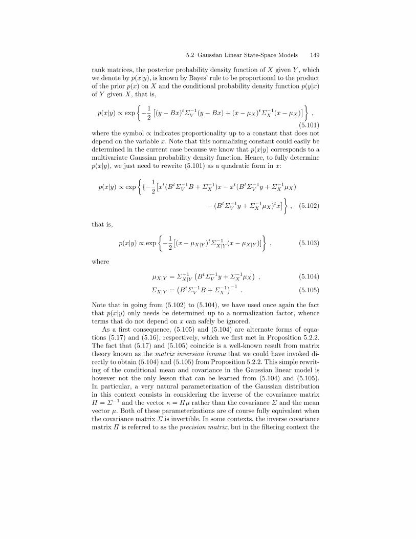
5.2 Gaussian Linear State-Space Models 149

rank matrices, the posterior probability density function of X given Y , whichwe denote by p(x|y), is known by Bayes’ rule to be proportional to the productof the prior p(x) on X and the conditional probability density function p(y|x)of Y given X, that is,

p(x|y) ∝ exp−1

2[(y −Bx)tΣ−1

V (y −Bx) + (x− µX)tΣ−1X (x− µX)

],

(5.101)where the symbol ∝ indicates proportionality up to a constant that does notdepend on the variable x. Note that this normalizing constant could easily bedetermined in the current case because we know that p(x|y) corresponds to amultivariate Gaussian probability density function. Hence, to fully determinep(x|y), we just need to rewrite (5.101) as a quadratic form in x:

p(x|y) ∝ exp−1

2[xt(BtΣ−1

V B +Σ−1X )x− xt(BtΣ−1

V y +Σ−1X µX)

− (BtΣ−1V y +Σ−1

X µX)tx]

, (5.102)

that is,

p(x|y) ∝ exp−1

2[(x− µX|Y )tΣ−1

X|Y (x− µX|Y )], (5.103)

where

µX|Y = Σ−1X|Y

(BtΣ−1

V y +Σ−1X µX

), (5.104)

ΣX|Y =(BtΣ−1

V B +Σ−1X

)−1. (5.105)

Note that in going from (5.102) to (5.104), we have used once again the factthat p(x|y) only needs be determined up to a normalization factor, whenceterms that do not depend on x can safely be ignored.

As a first consequence, (5.105) and (5.104) are alternate forms of equa-tions (5.17) and (5.16), respectively, which we first met in Proposition 5.2.2.The fact that (5.17) and (5.105) coincide is a well-known result from matrixtheory known as the matrix inversion lemma that we could have invoked di-rectly to obtain (5.104) and (5.105) from Proposition 5.2.2. This simple rewrit-ing of the conditional mean and covariance in the Gaussian linear model ishowever not the only lesson that can be learned from (5.104) and (5.105).In particular, a very natural parameterization of the Gaussian distributionin this context consists in considering the inverse of the covariance matrixΠ = Σ−1 and the vector κ = Πµ rather than the covariance Σ and the meanvector µ. Both of these parameterizations are of course fully equivalent whenthe covariance matrix Σ is invertible. In some contexts, the inverse covariancematrix Π is referred to as the precision matrix, but in the filtering context the

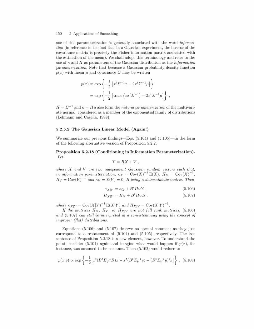
150 5 Applications of Smoothing

use of this parameterization is generally associated with the word informa-tion (in reference to the fact that in a Gaussian experiment, the inverse of thecovariance matrix is precisely the Fisher information matrix associated withthe estimation of the mean). We shall adopt this terminology and refer to theuse of κ and Π as parameters of the Gaussian distribution as the informationparameterization. Note that because a Gaussian probability density functionp(x) with mean µ and covariance Σ may be written

p(x) ∝ exp−1

2[xtΣ−1x− 2xtΣ−1µ

]= exp

−1

2[trace

(xxtΣ−1

)− 2xtΣ−1µ

],

Π = Σ−1 and κ = Πµ also form the natural parameterization of the multivari-ate normal, considered as a member of the exponential family of distributions(Lehmann and Casella, 1998).

5.2.5.2 The Gaussian Linear Model (Again!)

We summarize our previous findings—Eqs. (5.104) and (5.105)—in the formof the following alternative version of Proposition 5.2.2,

Proposition 5.2.18 (Conditioning in Information Parameterization).Let

Y = BX + V ,

where X and V are two independent Gaussian random vectors such that,in information parameterization, κX = Cov(X)−1 E(X), ΠX = Cov(X)−1,ΠV = Cov(V )−1 and κV = E(V ) = 0, B being a deterministic matrix. Then

κX|Y = κX +BtΠV Y , (5.106)

ΠX|Y = ΠX +BtΠVB , (5.107)

where κX|Y = Cov(X|Y )−1 E(X|Y ) and ΠX|Y = Cov(X|Y )−1.If the matrices ΠX , ΠV , or ΠX|Y are not full rank matrices, (5.106)

and (5.107) can still be interpreted in a consistent way using the concept ofimproper (flat) distributions.

Equations (5.106) and (5.107) deserve no special comment as they justcorrespond to a restatement of (5.104) and (5.105), respectively. The lastsentence of Proposition 5.2.18 is a new element, however. To understand thepoint, consider (5.101) again and imagine what would happen if p(x), forinstance, was assumed to be constant. Then (5.102) would reduce to

p(x|y) ∝ exp−1

2[xt(BtΣ−1

V B)x− xt(BtΣ−1V y)− (BtΣ−1

V y)tx]

, (5.108)

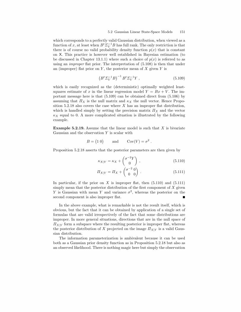
5.2 Gaussian Linear State-Space Models 151

which corresponds to a perfectly valid Gaussian distribution, when viewed as afunction of x, at least when BtΣ−1

V B has full rank. The only restriction is thatthere is of course no valid probability density function p(x) that is constanton X. This practice is however well established in Bayesian estimation (tobe discussed in Chapter 13.1.1) where such a choice of p(x) is referred to asusing an improper flat prior. The interpretation of (5.108) is then that underan (improper) flat prior on Y , the posterior mean of X given Y is(

BtΣ−1V B

)−1BtΣ−1

V Y , (5.109)

which is easily recognized as the (deterministic) optimally weighted least-squares estimate of x in the linear regression model Y = Bx + V . The im-portant message here is that (5.109) can be obtained direct from (5.106) byassuming that ΠX is the null matrix and κX the null vector. Hence Propo-sition 5.2.18 also covers the case where X has an improper flat distribution,which is handled simply by setting the precision matrix ΠX and the vectorκX equal to 0. A more complicated situation is illustrated by the followingexample.

Example 5.2.19. Assume that the linear model is such that X is bivariateGaussian and the observation Y is scalar with

B =(1 0)

and Cov(V ) = σ2 .

Proposition 5.2.18 asserts that the posterior parameters are then given by

κX|Y = κX +(σ−2Y

0

), (5.110)

ΠX|Y = ΠX +(σ−2 0

0 0

). (5.111)

In particular, if the prior on X is improper flat, then (5.110) and (5.111)simply mean that the posterior distribution of the first component of X givenY is Gaussian with mean Y and variance σ2, whereas the posterior on thesecond component is also improper flat.

In the above example, what is remarkable is not the result itself, which isobvious, but the fact that it can be obtained by application of a single set offormulas that are valid irrespectively of the fact that some distributions areimproper. In more general situations, directions that are in the null space ofΠX|Y form a subspace where the resulting posterior is improper flat, whereasthe posterior distribution of X projected on the image ΠX|Y is a valid Gaus-sian distribution.

The information parameterization is ambivalent because it can be usedboth as a Gaussian prior density function as in Proposition 5.2.18 but also asan observed likelihood. There is nothing magic here but simply the observation

152 5 Applications of Smoothing

that as we (i) allow for improper distributions and (ii) omit the normalizationfactors, Gaussian priors and likelihood are equivalent. The following lemmais a complement to Proposition 5.2.18, which will be needed below.

Lemma 5.2.20. Up to terms that do not depend on x,∫exp

−1

2[(y −Bx)tΣ−1(y −Bx)

]exp

−1

2[(ytΠy − 2ytκ

)]dy

∝ exp−1

2[xtBt(I +ΠΣ)−1ΠBx− 2xtBt(I +ΠΣ)−1κ

], (5.112)

where I denotes the identity matrix of suitable dimension.

Proof. The left-hand side of (5.112), which we denote by p(x), may be rewrit-ten as

p(x) = exp−1

2xBtΣ−1Bx

×∫

exp−12[yt(Π +Σ−1)y − 2yt(κ+Σ−1Bx)

]dy . (5.113)

Completing the square, the bracketed term in the integrand of (5.113) maybe written

y − (Π +Σ−1)−1(κ+Σ−1Bx)t

(Π +Σ−1)

×y − (Π +Σ−1)−1(κ+Σ−1Bx)

− (κ+Σ−1Bx)t(Π +Σ−1)−1(κ+Σ−1Bx) . (5.114)

The exponent of −1/2 times the first two lines of (5.114) integrates to aconstant (or, rather, a number not depending on x), as it is recognized as aGaussian probability density function. Thus

p(x) ∝ exp−12

[−2xtBtΣ−1(Π +Σ−1)−1κ

+ xtBt(Σ−1 −Σ−1(Π +Σ−1)−1Σ−1

)Bx

, (5.115)

where terms that do not depend on x have been dropped. Equation (5.112)follows from the equalities Σ−1(Π +Σ−1)−1 = (I +ΠΣ)−1 and

Σ−1 −Σ−1(Π +Σ−1)−1Σ−1

= Σ−1(Π +Σ−1)−1[(Π +Σ−1)−Σ−1

]= (I +ΠΣ)−1Π .

Note that the last identity is the matrix inversion lemma that we already met,as (I +ΠΣ)−1Π = (Π−1 +Σ)−1. Using this last form however is not a goodidea in general, however, as it obviously does not apply in cases where Π isnon-invertible. ut

5.2 Gaussian Linear State-Space Models 153

5.2.5.3 The Backward Recursion

The question now is, what is the link between our original problem, which con-sists in implementing the backward recursion in Gaussian linear state-spacemodels, and the information parameterization discussed in the previous sec-tion? The connection is the fact that the backward functions defined by (3.16)do not correspond to probability measures. More precisely, βk|n(Xk) definedby (3.16) is the conditional density of the “future” observations Yk+1, . . . , Yngiven Xk. For Gaussian linear models, we know from Proposition 5.2.18 thatthis density is Gaussian and hence that βk|n(x) has the form of a Gaussianlikelihood,

p(y|x) ∝ exp−12[(y −Mx)tΣ−1(y −Mx)

],

for some M and Σ given by (5.16) and (5.17). Proceeding as previously, thisequation can be put in the same form as (5.108) (replacing B and ΣV byM and Σ, respectively). Hence, a possible interpretation of βk|n(x) is thatit corresponds to the posterior distribution of Xk given Yk+1, . . . , Yn in thepseudo-model where Xk is assumed to have an improper flat prior distribution.According to the previous discussion, βk|n(x) itself may not correspond toa valid Gaussian distribution unless one can guarantee that M tΣ−1M is afull rank matrix. In particular, recall from Section 3.2.1 that the backwardrecursion is initialized by setting βn|n(x) = 1, and hence βn|n never is a validGaussian distribution.

The route from now on is clear: in order to implement the backward re-cursion, one needs to define a set of information parameters corresponding toβk|n and derive (backward) recursions for these parameters based on Propo-sition 5.2.18. We will denote by κk|n and Πk|n the information parameters(precision matrix times mean and precision matrix) corresponding to βk|n fork = n down to 0 where, by definition, κn|n = 0 and Πn|n = 0. It is importantto keep in mind that κk|n and Πk|n define the backward function βk|n onlyup to an unknown constant. The best we can hope to determine is

βk|n(x)∫βk|n(x) dx

,

by computing the Gaussian normalization factor in situations where Πk|n isa full rank matrix. But this normalization is not more legitimate or practicalthan other ones, and it is preferable to consider that βk|n will be determined upto a constant only. In most situations, this will be a minor concern, as formulasthat take into account this possible lack of normalization, such as (3.21), areavailable.

Proposition 5.2.21 (Backward Information Recursion). Consider theGaussian linear state-space model (5.11)–(5.12) and assume that SkStk hasfull rank for all k ≥ 0. The information parameters κk|n and Πk|n, whichdetermine βk|n (up to a constant), may be computed by the following recursion.

154 5 Applications of Smoothing

Initialization: Set κn|n = 0 and Πn|n = 0.Backward Recursion: For k = n− 1 down to 0,

κk+1|n = Btk+1

(Sk+1S

tk+1

)−1Yk+1 + κk+1|n , (5.116)

Πk+1|n = Btk+1

(Sk+1S

tk+1

)−1Bk+1 +Πk+1|n , (5.117)

κk|n = Atk

(I + Πk+1|nRkR

tk

)−1

κk+1|n , (5.118)

Πk|n = Atk

(I + Πk+1|nRkR

tk

)−1

Πk+1|nAk . (5.119)

Proof. The initialization of Proposition 5.2.21 has already been discussed andwe just need to check that (5.116)–(5.119) correspond to an implementationof the general backward recursion (Proposition 3.2.1).

We split this update in two parts and first consider computing

βk+1|n(x) ∝ gk+1(x)βk+1|n(x) (5.120)

from βk+1|n. Equation (5.120) may be interpreted as the posterior distribu-tion of X in the pseudo-model in which X has a (possibly improper) priordistribution βk+1|n (with information parameters κk+1|n and Πk+1|n) and

Y = Bk+1X + Sk+1V

is observed, where V is independent of X. Equations(5.116)–(5.117) thuscorrespond to the information parameterization of βk+1|n by application ofProposition 5.2.18.

From (3.19) we then have

βk|n(x) =∫Qk(x, dx′)βk+1|n(x′) , (5.121)

where we use the notation Qk rather than Q to emphasize that we are deal-ing with possibly non-homogeneous models. Given that Qk is a Gaussiantransition density function corresponding to (5.12), (5.121) may be computedexplicitly by application of Lemma 5.2.20 which gives (5.118) and (5.119). ut

While carrying out the backward recursion according to Proposition 5.2.21,it is also possible to simultaneously compute the marginal smoothing distri-bution by use of (3.21).

Algorithm 5.2.22 (Forward-Backward Smoothing).

Forward Recursion: Perform Kalman filtering according to Algorithm 5.2.13 andstore the values of Xk|k and Σk|k.

Backward Recursion: Compute the backward recursion, obtaining for each k themean and covariance matrix of the smoothed estimate as

Xk|n = Xk|k +Σk|k(I +Πk|nΣk|k

)−1 (κk|n −Πk|nXk|k) , (5.122)

Σk|n = Σk|k −Σk|k(I +Πk|nΣk|k

)−1Πk|nΣk|k . (5.123)

5.2 Gaussian Linear State-Space Models 155

Proof. These two equations can be obtained exactly as in the proof ofLemma 5.2.20, replacing (y − Bx)tΣ−1(y − Bx) by (x − µ)tΣ−1(x − µ) andapplying the result with µ = Xk|k, Σ = Σk|k, κ = κk|n and Π = Πk|n. IfΠk|n is invertible, (5.122) and (5.123) are easily recognized as the applicationof Proposition 5.2.2 with B = I, Cov(V ) = Π−1

k|n, and an equivalent observedvalue of Y = Π−1

k|nκk|n. ut

Remark 5.2.23. In the original work by Mayne (1966), the backward infor-mation recursion is carried out on the parameters of βk|n, as defined by (5.120),rather than on βk|n. It is easily checked using (5.116)–(5.119) that, except forthis difference of focus, Proposition 5.2.21 is equivalent to the Mayne (1966)formulas—see also Kailath et al. (2000, Section 10.4) on this point. Of course,in the work of Mayne (1966), βk|n has to be combined with the predictivedistribution φk|k−1 rather than with the filtering distribution φk, as βk|n al-ready incorporates the knowledge of the observation Yk. Proposition 5.2.21and Algorithm 5.2.22 are here stated in a form that is compatible with ourgeneral definition of the forward-backward decomposition in Section 3.2.

5.2.6 Application to Marginal Filtering and Smoothing inCGLSSMs

The algorithms previously derived for linear state-space models also haveimportant implications for conditionally Gaussian linear state-space models(CGLSSMs). According to Definition 2.2.6, a CGLSSM is such that condi-tionally on Ckk≥0,

Wk+1 = A(Ck+1)Wk +R(Ck+1)Uk , W0 ∼ N(µν , Σν) ,Yk = B(Ck)Wk + S(Ck)Vk ,

where the indicator process Ckk≥0 is a Markov chain on a finite set X, withsome transition matrix QC .

We follow the general principle outlined in Section 4.2.3 and consider thecomputation of the posterior distribution of the indicator variables C0:k giventhe observations Y0:k, marginalizing with respect to the continuous compo-nent of the state W0:k. The key remark—see (4.11)—is that one may evaluatethe conditional distribution of Wk given the observations Y0:k−1 and the indi-cator variables C0:k. For CGLSSMs, this distribution is Gaussian with meanWk|k−1(C0:k) and covariance Σk|k−1(C0:k)—the dependence on the measure-ment, here Y0:k−1, is implicit and we emphasize only the dependence withrespect to the indicator variables in the following. Both of these quantitiesmay be evaluated using the Kalman filter recursion (Algorithm 5.2.13), whichwe briefly recall here.

Given Wk−1|k−1(C0:k−1) and Σk−1|k−1(C0:k−1), the filtered partial stateestimator and the filtered partial state error covariance at time k−1, evaluate

156 5 Applications of Smoothing

the predicted partial state and the associated predicted partial state errorcovariance as

Wk|k−1(C0:k) = A(Ck)Wk−1|k−1(C0:k−1) , (5.124)

Σk|k−1(C0:k) = A(Ck)Σk−1|k−1(C0:k−1)At(Ck) +R(Ck)Rt(Ck) .

From these quantities, determine in a second step the innovation and thecovariance of the innovation given the indicator variables,

εk(C0:k) = Yk −B(Ck)Wk|k−1(C0:k) , (5.125)

Γk(C0:k) = B(Ck)Σk|k−1(C0:k)Bt(Ck) + S(Ck)St(Ck) .

In a third and last step, evaluate the filtered partial state estimation andfiltered partial state error covariance from the innovation and the innovationcovariance,

Kk(C0:k) = Σk|k−1(C0:k)B(Ck)Γ−1k (C0:k) , (5.126)

Wk|k(C0:k) = Wk|k−1(C0:k) +Kk(C0:k)εk(C0:k) ,Σk|k(C0:k) = I −Kk(C0:k)B(Ck) Σk|k−1(C0:k) .

As a by-product of the above recursion, one may also determine the condi-tional probability of Ck given the history of the indicator process C0:k−1 andthe observations Y0:k up to index k. Indeed, by Bayes’ rule,

Pν(Ck = c |C0:k−1, Y0:k)Pν(Ck = c′ |C0:k−1, Y0:k)

=

Lν(Y0:k |C0:k−1, Ck = c)QC(Ck−1, c)Lν(Y0:k |C0:k−1, Ck = c′)QC(Ck−1, c′)

, (5.127)

where Lν denotes the conditional likelihood of the observations given the in-dicator variables. Both the numerator and the denominator can be evaluated,following Remark (5.2.10), by applying the Kalman recursions (5.125)–(5.126)for the two values Ck = c and Ck = c′. Using (5.62) and (5.127) then yields

Pν(Ck = c |C0:k−1, Y0:k) ∝ |Γk(C0:k−1, c)|−1/2×

exp−1

2εtk(C0:k−1, c)Γ−1

k (C0:k−1, c)εk(C0:k−1, c)QC(Ck−1, c) , (5.128)

where the normalization factor may be evaluated by summation of (5.128)over all c ∈ C. At the expense of computing r times (5.125)–(5.126), wherer is the cardinality of C, it is thus possible to evaluate the conditional dis-tribution of Ck given the history of the indicator process C0:k−1, where thecontinuous variables W0:k have been fully marginalized out. To be applicablehowever, (5.128) implies that the history of the indicator process before in-dex k be exactly known. This is hardly conceivable except in simulation-based

5.2 Gaussian Linear State-Space Models 157

smoothing approximations where one imputes values of the unknown sequenceof indicators Ckk≥0. The application of (5.125)–(5.126) and (5.128) for thispurpose will be fully described in Chapter 8.

A similar remark holds regarding the computation of the conditional distri-bution of Ck given both the history C0:k−1 and future Ck+1:n of the indicatorsequence and the corresponding observations Y0:n. The principle that we followhere is an instance of the generalized forward-backward decomposition (4.13)which, in the case of CGLSSMs, amounts to adapting Algorithm 5.2.22 asfollows.

1. Use the backward information recursion of Proposition 5.2.21 to computeκk|n(Ck+1:n) and Πk|n(Ck+1:n)2.

2. Use the filtering recursion of Algorithm 5.2.13—restated above as (5.124)–(5.126)—to compute Wk−1|k−1(C0:k−1) and Σk−1|k−1(C0:k−1).

3. For all values of c ∈ C, evaluate εk(C0:k−1, c), Γk(C0:k−1, c), as wellas Wk|k(C0:k−1, c), Σk|k(C0:k−1, c) using one step of Algorithm 5.2.13.Then apply (5.122) and (5.123) to obtain Wk|n(C0:k−1, c, Ck+1:n) andΣk|n(C0:k−1, c, Ck+1:n).

The most difficult aspect then consists in computing the likelihood of theobservations Y0:n given the indicator sequence, where all indicators variablesbut ck are fixed and ck takes all possible values in C. The lemma below providesa simple formula for this task.

Lemma 5.2.24. Assume that εk(ck), Γk(ck), Wk|k(ck), Σk|k(ck), Wk|n(ck),and Σk|n(ck) are available, where we omit dependence with respect to the in-dicator variables cl for l 6= k, which is implicit in the following.

The likelihood of the observations Y0:n given the indicator sequence C0:n =c0:n is then proportional to the quantity

1|Γk(ck)|1/2

exp[−1

2εtk(ck)Γ−1

k (ck)εk(ck)]

× 1|Σk|k(ck)|1/2

exp[−1

2W tk|k(ck)Σ−1

k|k(ck)Wk|k(ck))]

×

1|Σk|n(ck)|1/2

exp[−1

2W tk|n(ck)Σ−1

k|n(ck)Wk|n(ck))]−1

, (5.129)

where the proportionality constant does not depend on the value of ck.

Before actually proving this identity, we give a hint of the fundamentalargument behind (5.129). If X and Y are jointly Gaussian variables (withnon-singular covariance matrices), Bayes’ rule implies that

2We do not repeat Proposition 5.2.21 with the notations appropriate forCGLSSMs as we did for (5.124)–(5.126).

158 5 Applications of Smoothing

p(x|y) =p(y|x)p(x)∫p(y|x′)p(x′) dx′

.

In particular, the denominator on the right-hand side equals p(y|x)p(x)/p(x|y)for any value of x. For instance, in the linear model of Proposition 5.2.2,applying this identity for x = 0 yields∫

p(Y |x)p(x) dx ∝ 1|ΣV |1/2

exp[−1

2Y tΣ−1

V Y

]× 1|ΣX |1/2

exp[−1

2µtXΣ

−1X µX

]×

1|ΣX|Y |1/2

exp[−1

2µtX|YΣX|Y µX|Y

]−1

, (5.130)

where µX|Ydef= E(X|Y ) and ΣX|Y

def= Cov(X|Y ) and constants have beenomitted. It is tedious but straightforward to check from (5.16) and (5.17)using the matrix inversion lemma that (5.130) indeed coincides with what weknow to be the correct result:∫

p(Y |x)p(x) dx = p(Y ) ∝

1|ΣV +BΣXBt|1/2

exp[−1

2(Y −BµX)t(ΣV +BΣXB

t)−1(Y −BµX)].

Equation (5.130) is certainly not the most efficient way of computing p(Y )but it is one that does not necessitate any other knowledge than that of theprior p(x), the conditional p(y|x), and the posterior p(x|y). Lemma 5.2.24 willnow be proved by applying the same principle to the conditional smoothingdistribution in a CGLSSM.

Proof (Conditional Smoothing Lemma). The forward-backward decomposi-tion provides a simple general expression for the likelihood of the observationsY0:n in the form

Ln =∫αk(dw)βk|n(w) (5.131)

for any k = 0, . . . , n. Recall that our focus is on the likelihood of the obser-vations conditional on a given sequence of indicator variables C0:n = c0:n,and more precisely on the evaluation of the likelihood for all values of ck inC, the other indicator variables cl, l 6= k, being held fixed. In the following,every expression should be understood as being conditional on C0:n = c0:n,where only the dependence with respect to ck is of interest (terms that do notdepend on the value of ck will cancel out by normalization). This being said,(5.131) may be rewritten as

L(ck)n =

∫∫αk−1(dwk−1)Q(ck)(wk−1, dwk)g(ck)

k (wk)βk|n(wk) (5.132)

5.2 Gaussian Linear State-Space Models 159

using the forward recursion (3.17), where the superscript (ck) is used to high-light quantities that depend on this variable. Because the first term of theintegrand does not depend on ck, it may be replaced by its normalized ver-sion φk−1 to obtain

L(ck)n ∝

∫∫φk−1(dwk−1)Q(ck)(wk−1, dwk)g(ck)

k (wk)βk|n(wk) , (5.133)

where the proportionality constant does not depend on ck. Now, using theprediction and filtering relations (see Proposition 3.2.5 and Remark 3.2.6),the right-hand side of (5.133) may be rewritten as the product∫

φ(ck)k|k−1(dw)g(ck)

k (w)×∫φ

(ck)k (dw)βk|n(w) . (5.134)

Finally note that in the case of conditionally Gaussian linear state-space mod-els: (i) the first integral in (5.134) may be computed from the innovation εk asthe first line of (5.129)—a remark that was already used in obtaining (5.128);(ii) φ(ck)

k is a Gaussian probability density function with parameters Wk|k(ck)and Σk|k(ck); (iii) βk|n is a Gaussian likelihood defined, up to a constant, bythe information parameters κk|n and Πk|n;

(iv) φ(ck)k|n (dw) =

φ(ck)k (dw)βk|n(w)∫φ

(ck)k (dw′)βk|n(w′)

is the Gaussian distribution with parameters Xk|n and Σk|n given by (5.122)and (5.123), respectively. The last two factors of (5.129) are now easily recog-nized as an instance of (5.130) applied to the second integral term in (5.134),where the factor βk|n(0) has been ignored because it does not depend on thevalue of ck. Note that as a consequence, the fact that κk|n and Πk|n defineβk|n up to an unknown constant only is not detrimental. ut

Once again, the context in which Lemma 5.2.24 will be useful is not en-tirely obvious at this point and will be fully discussed in Section 6.3.2 whenreviewing Monte Carlo methods. From the proof of this result, it should beclear however that (5.129) is deeply connected to the smoothing approachdiscussed in Section 5.2.5 above.

6

Monte Carlo Methods

This chapter takes a different path to the study of hidden Markov models inthat it abandons the pursuit of closed-form formulas and exact algorithms tocover instead simulation-based techniques. This change of perspective allowsfor a much broader coverage of HMMs, which is not restricted to the specificcases discussed in Chapter 5. In this chapter, we consider sampling the un-known sequence of states X0, . . . , Xn conditionally on the observed sequenceY0, . . . Yn. In subsequent chapters, we will also use simulation to do inferenceabout the parameters of HMMs, either using simulation-based stochastic algo-rithms that optimize the likelihood (Chapter 11) or in the context of Bayesianjoint inference on the states and parameters (Chapter 13). But even the solesimulation of the missing states may prove itself a considerable challenge incomplex settings like continuous state-space HMMs. Therefore, and althoughthese different tasks are presented in separate chapters, simulating hiddenstates in a model whose parameters are assumed to be known is certainlynot disconnected from parameter estimation to be discussed in Chapters 11and 13.

6.1 Basic Monte Carlo Methods

Although we will not go into a complete description of simulation methodsin this book, the reader must be aware that recent developments of thesemethods have offered new opportunities for inference in complex models likehidden Markov models and their generalizations. For a more in-depth coveringof these simulation methods and their implications see, for instance, the booksby Chen and Shao (2000), Evans and Swartz (2000), Liu (2001), and Robertand Casella (2004).

162 6 Monte Carlo Methods

6.1.1 Monte Carlo Integration

Integration, in general, is most useful for computing probabilities and expec-tations. Of course, when given an expectation to compute, the first thing isto try to compute the integral analytically. When analytic evaluation is im-possible, numerical integration is an option. However, especially when thedimension of the space is large, numerical integration can become numericallyinvolved: the number of function evaluations required to achieve some degreeof approximation increases exponentially in the dimension of the problem (thisis often called the curse of dimensionality).

Thus it is useful to consider other methods for evaluating integrals. For-tunately, there are methods that do not suffer so directly from the curse ofdimensionality, and Monte Carlo methods belong to this group. In particular,recall that, by the strong law of large numbers, if ξ1, ξ2, . . . is a sequence ofi.i.d. X-valued random variables with common probability distribution π, thenthe estimator

πMCN (f) = N−1

N∑i=1

f(ξi)

converges almost surely to π(f) for all π-integrable functions f . Obviouslythis Monte Carlo estimate of the expectation is not exact, but generating asufficiently large number of random variables can render this approximationerror arbitrarily small, in a suitable probabilistic sense. It is even possible toassess the size of this error. If

π(|f |2) =∫|f(x)|2 π(dx) <∞ ,

the central limit theorem shows that√N[πMCN (f)− π(f)

]has an asymptotic

normal distribution, which can be used to construct asymptotic confidenceregions for π(f). For instance, if f is real-valued, a confidence interval withasymptotic probability of coverage α is given by[

πMCN (f)− cαN−1/2σN (π, f), πMC

N (f) + cαN−1/2σN (π, f)

], (6.1)

where

σ2N (π, f) def= N−1

N∑i=1

[f(ξi)− πMC

N (f)]2

and cα is the α/2 quantile of the standard Gaussian distribution. If generatinga sequence of i.i.d. samples from π is practicable, one can make the confidenceinterval as small as desired by increasing the sample size N . When comparedto univariate numerical integration and quasi-Monte Carlo methods (Nieder-reiter, 1992), the convergence rate is not fast. In practical terms, (6.1) impliesthat an extra digit of accuracy on the approximation requires 100 times asmany replications, where the rate 1/

√N cannot be improved. On the other

6.1 Basic Monte Carlo Methods 163

hand, it is possible to derive methods to reduce the asymptotic variance of theMonte Carlo estimate by allowing a certain amount of dependence among therandom variables ξ1, ξ2, . . . Such methods include antithetic variables, controlvariates, stratified sampling, etc. These techniques are not discussed here (seefor instance Robert and Casella, 2004, Chapter 4). A remarkable fact howeveris that the rate of convergence of 1/

√N in (6.1) remains the same whatever

the dimension of the space X is, which leaves some hope of effectively usingthe Monte Carlo approach in large-dimensional settings.

6.1.2 Monte Carlo Simulation for HMM State Inference

6.1.2.1 General Markovian Simulation Principle

We now turn to the specific task of simulating the unobserved sequence ofstates in a hidden Markov model, given some observations. The main re-sult has already been discussed in Section 3.3: given some observations, theunobserved sequence of states constitutes a non-homogeneous Markov chainwhose transition kernels may be evaluated, either from the backward func-tions for the forward chain (with indices increasing as usual) or from theforward measures—or equivalently filtering distributions—for the backwardchain (with indices in reverse order). Schematically, both available optionsare rather straightforward to implement.

Backward Recursion/Forward Sampling: First compute (and store) the back-ward functions βk|n by backward recursion, for k = n, n − 1 down to 0(Proposition 3.2.1). Then, simulate Xk+1 given Xk from the forward tran-sition kernels Fk|n specified in Definition 3.3.1.

Forward Recursion/Backward Sampling: First compute and store the forwardmeasures αν,k by forward recursion, according to Proposition 3.2.1. As analternative, one may evaluate the normalized versions of the forward mea-sures, which coincide with the filtering distributions φν,k, following Propo-sition 3.2.5. Then Xk is simulated conditionally on Xk+1 (starting fromXn) according to the backward transition kernel Bν,k defined by (3.38).

Despite its beautiful simplicity, the method above will obviously be of no helpin cases where an exact implementation of the forward-backward recursion isnot available.

6.1.2.2 Models with Finite State Space

In the case where the state space X is finite, the implementation of the forward-backward recursions is feasible and has been fully described in Section 5.1.The second method described above is a by-product of Algorithm 5.1.3.

Algorithm 6.1.1 (Markovian Backward Sampling). Given the stored val-ues of φ0, . . . , φn computed by forward recursion according to Algorithm 5.1.1,do the following.

164 6 Monte Carlo Methods

Final State: Simulate Xn from φn.

Backward Simulation: For k = n−1 down to 0, compute the backward transitionkernel according to (5.7) and simulate Xk from Bk(Xk+1, ·).

The numerical complexity of this sampling algorithm is thus equivalent tothat of Algorithm 5.1.3, whose computational cost depends most importantlyon the cardinal r of X and on the difficulty of evaluating the function g(x, Yk)for all x ∈ X and k = 0, . . . , n (see Section 5.1). The backward simulationpass in Algorithm 6.1.1 is simpler than its smoothing counterpart in Algo-rithm 5.1.3, as one only needs to evaluate Bk(Xk+1, ·) for the simulated valueof Xk+1 rather than Bk(i, j) for all (i, j) ∈ 1, . . . , r2.

6.1.2.3 Gaussian Linear State-Space Models

As discussed in Section 5.2, Rauch-Tung-Striebel smoothing (Algorithm 5.2.4)is the exact counterpart of Algorithm 5.1.3 in the case of Gaussian linear state-space models. Not surprisingly, to obtain the smoothing means and covariancematrices in Algorithm 5.2.4, we explicitly constructed the backward Gaussiantransition density, whose mean and covariance are given by (5.23) and (5.24),respectively. We simply reformulate this observation in the form of an algo-rithm as follows.

Algorithm 6.1.2 (Gaussian Backward Markovian State Sampling).Assume that the filtering moments Xk|k and Σk|k have been computed usingProposition 5.2.3. Then do the following.

Final State: SimulateXn ∼ N(Xn|n, Σn|n).

Backward Simulation: For k = n − 1 down to 0, simulate Xk from a Gaussiandistribution with mean and covariance matrix given by (5.23) and (5.24),respectively.

The limitations discussed in the beginning of Section 5.2.2 concerning RTSsmoothing (Algorithm 5.2.4) also apply here. In some models, Algorithm 6.1.2is far from being computationally efficient (Fruhwirth-Schnatter, 1994; Carterand Kohn, 1994). With these limitations in mind, De Jong and Shephard(1995) described a sampling algorithm inspired by disturbance (or Bryson-Frazier) smoothing (Algorithm 5.2.15) rather than by RTS smoothing. Themethod of De Jong and Shephard (1995) is very close to Algorithm 5.2.15and proceeds by sampling the disturbance vectors Uk backwards (for k =n− 1, . . . , 0) and then the initial state X0, from which the complete sequenceX0:n may be obtained by repeated applications of the dynamic equation (5.11).Because the sequence of disturbance vectors Ukk=n−1,...,0 does not howeverhave a backward Markovian structure, the method of De Jong and Shephard(1995) is not a simple by-product of disturbance smoothing (as was the case

6.1 Basic Monte Carlo Methods 165

for Algorithms 5.2.4 and 6.1.2). Durbin and Koopman (2002) described anapproach that is conceptually simpler and usually about as efficient as thedisturbance sampling method of De Jong and Shephard (1995).

The basic remark is that if X and Y are jointly Gaussian variables, theconditional distribution of X given Y is Gaussian with mean vector E [X |Y ]and covariance matrix Cov(X |Y ), where Cov(X |Y ) equals Cov(X−E[X |Y ])and, in addition, does not depend on Y (Proposition 5.2.2). In particular, if(X∗, Y ∗) is another independent pair of Gaussian distributed random vectorswith the same (joint) distribution, X−E[X |Y ] and X∗−E[X∗ |Y ∗] are inde-pendent and both are N (0,Cov(X |Y )) distributed. In summary, to simulateξ from the distribution of X given Y , one may

1. Simulate an independent pair of Gaussian variables (X∗, Y ∗) with thesame distribution as (X,Y ) and compute X∗ − E[X∗ |Y ∗];

2. Given Y , compute E[X |Y ], and set

ξ = E[X |Y ] +X∗ − E[X∗ |Y ∗] .

This simulation approach only requires the ability to compute conditionalexpectations and to simulate from the prior joint distribution of X and Y .When applied to the particular case of Gaussian linear state-space models,this general principle yields the following algorithm.

Algorithm 6.1.3 (Sampling with Dual Smoothing). Given a Gaussianlinear state-space model following (5.11)–(5.12) and observations Y0, . . . , Yn, dothe following.

1. Simulate a fictitious independent sequence X∗k , Y ∗k k=0,...,n of both statesand observations using the model equations.

2. Compute Xk|nk=0,...,n and X∗k|nk=0,...,n using Algorithm 5.2.15 for the

two sequences Ykk=0,...,n and Y ∗k k=0,...,n.

Then Xk|n + X∗k − X∗k|nk=0,...,n is distributed according to the posterior dis-tribution of the states given Y0, . . . , Yn.

Durbin and Koopman (2002) list a number of computational simplifica-tions that are needed to make the above algorithm competitive with the distur-bance sampling approach. As already noted in Remark 5.2.16, the backwardrecursion of Algorithm 5.2.15 may be greatly simplified when only the bestlinear estimates (and not their covariances) are to be computed. During theforward Kalman prediction recursion, it is also possible to save on computa-tions by noting that all covariance matrices (state prediction error, innovation)will be common for the two sequences Yk and Y ∗k , as these matrices donot depend on the observations but only on the model. The same remarkshould be used when the purpose is not only to simulate one sequence but Nsequences of states conditional on the same observations, which will be thestandard situation in a Monte Carlo approach. Further improvement can be

166 6 Monte Carlo Methods

gained by carrying out simultaneously the simulation and Kalman predictiontasks, as both of them are implemented recursively (Durbin and Koopman,2002).

6.2 A Markov Chain Monte Carlo Primer

As we have seen above, the general task of simulating the unobserved X0:n

given observations Y0:n is non-trivial except when X in finite or the model is aGaussian linear state-space model. In fact, in such models, analytic integrationwith respect to (low-dimensional marginals of) the conditional distributionof X0:n given observations is most often feasible, whence there is generallyno true need for simulation of the unobserved Markov chain. The importantand more difficult challenge is rather to explore methods to carry out thistask in greater generality, and this is the object of the current section. Westart by describing the accept-reject algorithm, which is a general approachto simulation of i.i.d. samples from a prescribed distribution, and then turnto so-called Markov chain Monte Carlo methods, which are generally moresuccessful in large-dimensional settings.

6.2.1 The Accept-Reject Algorithm

For specific distributions such as the Gaussian, Poisson, or Gamma distribu-tions, there are efficient tailor-made simulation procedures; however, we shallnot discuss here the most basic (but nonetheless essential) aspects of randomvariate generation for which we refer, for instance, to the books by Devroye(1986), Ripley (1987), or Gentle (1998). We are rather concerned with meth-ods that can provide i.i.d. samples from any pre-specified distribution π, notjust for specific choices of this distribution. It turns out that there are onlya limited number of options for this task, which include the accept-reject al-gorithm discussed here and the sampling importance resampling approach tobe discussed in Section 7.1 (although the latter only provides an approximatei.i.d. sample).

The accept-reject algorithm, first described by von Neumann, is importantboth for its direct applications and also because its principle is at the coreof many of the more advanced methods to be discussed in the following (forgeneral references on the accept-reject method, see Devroye, 1986, Chapter 2,Ripley, 1987, p. 60–62, or Robert and Casella, 2004, Chapter 2). It is easierto introduce the key concepts using probability densities, and we assume thatπ has a density with respect to a measure λ; because this assumption willbe adopted all through this section, we shall indeed use the notation π forthis density as well. The key requirement of the method is the availability ofanother probability density function (with respect to λ) r whose functionalform is known and from which i.i.d. sampling is readily feasible. We also

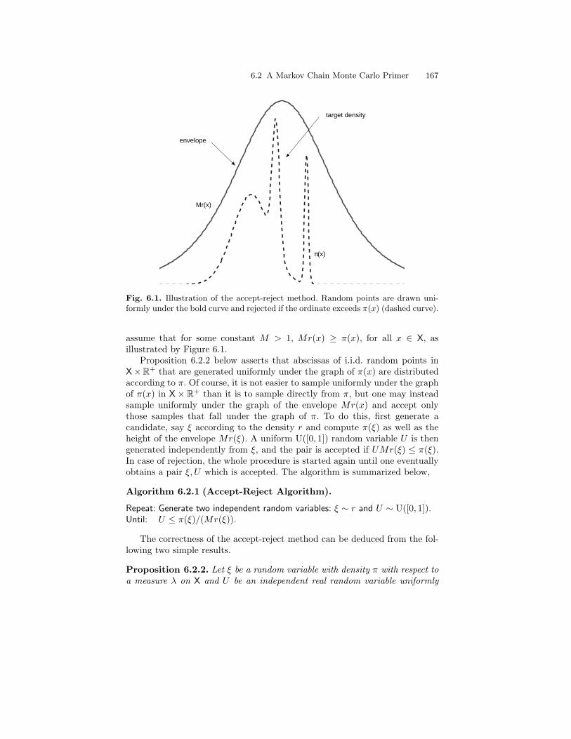
6.2 A Markov Chain Monte Carlo Primer 167

envelope

Mr(x)

target density

π(x)

Fig. 6.1. Illustration of the accept-reject method. Random points are drawn uni-formly under the bold curve and rejected if the ordinate exceeds π(x) (dashed curve).

assume that for some constant M > 1, Mr(x) ≥ π(x), for all x ∈ X, asillustrated by Figure 6.1.

Proposition 6.2.2 below asserts that abscissas of i.i.d. random points inX×R+ that are generated uniformly under the graph of π(x) are distributedaccording to π. Of course, it is not easier to sample uniformly under the graphof π(x) in X × R+ than it is to sample directly from π, but one may insteadsample uniformly under the graph of the envelope Mr(x) and accept onlythose samples that fall under the graph of π. To do this, first generate acandidate, say ξ according to the density r and compute π(ξ) as well as theheight of the envelope Mr(ξ). A uniform U([0, 1]) random variable U is thengenerated independently from ξ, and the pair is accepted if UMr(ξ) ≤ π(ξ).In case of rejection, the whole procedure is started again until one eventuallyobtains a pair ξ, U which is accepted. The algorithm is summarized below,

Algorithm 6.2.1 (Accept-Reject Algorithm).

Repeat: Generate two independent random variables: ξ ∼ r and U ∼ U([0, 1]).Until: U ≤ π(ξ)/(Mr(ξ)).

The correctness of the accept-reject method can be deduced from the fol-lowing two simple results.

Proposition 6.2.2. Let ξ be a random variable with density π with respect toa measure λ on X and U be an independent real random variable uniformly

168 6 Monte Carlo Methods

distributed on the interval [0,M ]. Then the pair (ξ, Uπ(ξ)) of random variablesis uniformly distributed on

Sπ,M =

(x, u) ∈ X× R+ : 0 < u < Mπ(x),

with respect to λ⊗ λLeb, where λLeb denotes Lebesgue measure.Conversely, if a random vector (ξ, U) of X × R+ is uniformly distributed

on Sπ,M , then ξ admits π as marginal probability density function.

Proof. Obviously, if Proposition 6.2.2 is to be true for some value of M0, thenboth claims also hold for all values of M > 0 simply by scaling the ordinateby M/M0. In the following, we thus consider the case where M equals one.For the first statement, take a measurable subset B ⊆ Sπ,1 and let Bx denotethe section of B in x, that is, Bx = u : (x, u) ∈ B. Then

P (ξ, Uπ(ξ)) ∈ B =∫x∈X

∫u∈Bx

1π(x)

λLeb(du)π(x)λ(dx) =∫∫

B

λLeb(du)λ(dx) .

For the second statement, consider a measurable subset A ⊆ X and set A =(x, u) ∈ A× R+ : 0 ≤ u ≤ π(x). Then

P(ξ ∈ A) = P((ξ, U) ∈ A

)=

∫∫AλLeb(du)λ(dx)∫∫

Sπ,1λLeb(du)λ(dx)

=∫A

π(x)λ(dx) .

ut

Lemma 6.2.3. Let V1, V2, . . . be a sequence of i.i.d. random variables takingvalues in a measurable space (V,V) and B ∈ V a set such that P(V1 ∈ B) =p > 0.

The integer-valued random variable σ = inf k ≥ 1, Vk ∈ B (with the con-vention that inf ∅ =∞) is geometrically distributed with parameter p, i.e., forall i ≥ 0,

P(σ = i) = (1− p)i−1p . (6.2)

The random variable V = Vσ1σ<∞ is distributed according to

P(V ∈ A) =P(V ∈ A ∩B)

p. (6.3)

Proof. First note that

P(σ = i) = P(V1 6∈ B, . . . , Vi−1 6∈ B, Vi ∈ B) = (1− p)i−1p ,

showing (6.2), which implies in particular that the waiting time σ is finitewith probability one. For A ∈ V,

6.2 A Markov Chain Monte Carlo Primer 169

P(V ∈ A) =∞∑i=1

P(V1 6∈ B, . . . , Vi−1 6∈ B, Vi ∈ A ∩B)

=∞∑i=1

(1− p)i−1 P(V1 ∈ A ∩B)

= P(V1 ∈ A ∩B)1

1− (1− p).

ut

Hence by Proposition 6.2.2, the intermediate pairs (ξi, Ui) generated inAlgorithm 6.2.1 are such that (ξi,MUir(ξi)) are uniformly distributed underthe graph of Mr(x). By Lemma 6.2.3, the accepted pair (ξ, U) is then uni-formly distributed under the graph of π(x) and, using Proposition 6.2.2, ξis marginally distributed according to π. The probability p of acceptance isequal to

PU1 ≤

π(ξ1)Mr(ξ1)

= P (ξ1,MU1r(ξ1)) ∈ Sπ,M =

∫Xπ(x)λ(dx)∫

XMr(x)λ(dx)

=1M

.

Remark 6.2.4. The same algorithm can be applied also in cases where thedensities π or r are known only up to a constant. In that case, denote byCπ =

∫π(x)λ(dx) and Cr =

∫r(x)λ(dx) the normalizing constants. The con-

dition π(x) ≤ Mr(x) can be equivalently written as π(x) ≤ M(Cr/Cπ)r(x),where π(x) = π(x)/Cπ and r(x) = r(x)/Cr denote the actual probability den-sity functions. Because the two stopping conditions π(x) ≤ M(Cr/Cπ)r(x)and π(x) ≤ Mr(x) are equivalent, using the accept-reject algorithm with π,r, and M amounts to using it with π, r and MCr/Cπ. Therefore, the knowl-edge of the normalizing constants Cπ and Cr is not required. Note howeverthat when either Cπ or Cr differs from one, it is not possible anymore tointerpret 1/M as the acceptance probability, and the actual acceptance prob-ability Cπ/(CrM) is basically unknown. In that case, the complexity of theaccept-reject algorithm (typically how many intermediate draws are requiredon average before accepting a single one) cannot be determined in advanceand may only be estimated empirically.

Of course, the assumption π(x) ≤ Mr(x) puts some stringent constraintson the choice of the density r from which samples are drawn. The density rshould have both heavier tails and sharper infinite peaks than π. The efficiencyof the algorithm is the ratio of the areas under the two graphs of π(x) andMr(x), which equals 1/M . Therefore, it is essential to keep M as close to oneas possible. The optimal choice of M for a given r is Mr = supx∈X π(x)/r(x),as it maximizes the acceptance probability and therefore minimizes the av-erage required computational effort. Determining a proposal density r suchthat Mr is small and evaluating Mr (or a tight upper bound for it) are the

170 6 Monte Carlo Methods

two key ingredients for practical application of the accept-reject method. Inmany situations, and especially in multi-dimensional settings, both of thesetasks are often equally difficult (see Robert and Casella, 2004, for examples).

6.2.2 Markov Chain Monte Carlo

The remarks above highlight that although accept-reject is often a viableapproach in low-dimensional problems, it has serious drawbacks in large-dimensional ones. Most fortunately, there exists a class of alternatives thatallow us to handle arbitrary distributions, on large-dimensional sets, withouta detailed study of them. This class of simulation methods is called Markovchain Monte Carlo (or MCMC) methods, as they rely on Markov-dependentsimulations. It should be stressed at this point that the “Markov” in “Markovchain Monte Carlo” has nothing to do with the “Markov” in “hidden Markovmodels”. These MCMC methods are generic/universal and, while they natu-rally apply in HMM settings, they are by no means restricted to those.

The original MCMC algorithm was introduced by Metropolis et al. (1953)for the purpose of optimization on a discrete state space, in connection withstatistical physics: the paper was actually published in the Journal of ChemicalPhysics. The Metropolis algorithm was later generalized by Hastings (1970)and Peskun (1973, 1981) to statistical simulation. Despite several other papersthat highlighted its usefulness in specific settings (see, for example, Gemanand Geman, 1984; Tanner and Wong, 1987; Besag, 1989), the starting pointfor an intensive use of MCMC methods by the statistical community can betraced to the presentation of the Gibbs sampler by Gelfand and Smith (1990).The MCMC approach is now well-known in many scientific domains, whichinclude physics and statistics but also biology, engineering, etc.

Returning for a while to the general case where π is a distribution, thetenet of MCMC methods is the remark that simulating an i.i.d. sequenceξ1, . . . , ξn with common probability distribution π is not the only way to ap-proximate π in the sense of being able to approximate the expectation of anyπ-integrable function f . In particular, one may consider Markov-dependent se-quences ξii≥1 rather than i.i.d. sequences. The ergodic theorem for Markovchains asserts that, under suitable conditions (discussed in Section 14.2.6 ofChapter 14),

πMCMCN (f) =

1N

N∑i=1

f(ξi) (6.4)

is a reasonable estimate of the expectation of f under the stationary distribu-tion of the chain ξii≥1, for all integrable functions f . In addition, the rate ofconvergence is identical to that of standard (independent) Monte Carlo, thatis, 1/

√N . To make this idea practicable however requires simulation schemes

that guarantee

(i) that simulating the chain ξii≥1 given an arbitrary initial value ξ1 is aneasily implementable process;

6.2 A Markov Chain Monte Carlo Primer 171

(ii) that the stationary distribution of ξii≥1 indeed coincides with the de-sired distribution π;

(iii) that the chain ξii≥1 satisfies conditions needed to guarantee the con-vergence towards π, irrespectively of the initial value ξ1.

We will introduce below two major classes of such algorithms, and we referthe reader to Robert and Casella (2004) and Roberts and Tweedie (2005) foran appropriate detailed coverage of these MCMC methods.

In this context, the specific distribution of interest is generally referred toas the target distribution. To keep the presentation simple, we will also assumethat all distributions and conditional distributions arising are dominated by acommon measure λ. The target distribution in particular is assumed to havea probability density function, as above denoted by π, with respect to λ.

6.2.3 Metropolis-Hastings

The (very limited) assumption underlying the Metropolis-Hastings algorithm,besides the availability of π, is that one can simulate from a transition densityfunction r (with respect to the same measure λ), called the proposal distribu-tion, whose functional form is also known.

Algorithm 6.2.5 (The Metropolis-Hastings Algorithm). Simulate asequence of values ξii≥1, which forms a Markov chain on X, with the followingmechanism: given ξi,

1. Generate ξ ∼ r(ξi, ·);2. Set

ξi+1 =

ξ with probability α(ξi, ξ) def=π(ξ) r(ξ, ξi)π(ξi) r(ξi, ξ)

∧ 1

ξi otherwise(6.5)

The initial value ξ1 may be chosen arbitrarily.

In practice, (6.5) is carried out by drawing an independent U([0, 1]) vari-able U and accepting ξ only if U ≤ A(ξi, ξ), where

A(ξi, ξ) =π(ξ) r(ξ, ξi)π(ξi) r(ξi, ξ)

,

is generally referred to as the Metropolis-Hastings acceptance ratio.The reason for this specific choice of acceptance probability in (6.5), whose

name follows from Metropolis et al. (1953) and Hastings (1970), is that theassociated Markov chain ξt satisfies the detailed balance equation (2.12)discussed in Chapter 2.

Proposition 6.2.6 (Reversibility of the Metropolis-Hastings Kernel).The chain ξii≥1 generated by Algorithm 6.2.5 is reversible and π is its

stationary probability density function.

172 6 Monte Carlo Methods

Proof. The transition kernel K associated with Algorithm 6.2.5 is such thatfor a function f ∈ Fb (X),

K(x, f) =∫f(x′) [α(x, x′)r(x, x′)λ(dx′) + pR(x) δx(dx′)] ,

where pR(x) is the probability of remaining in the state x, given by

pR(x) = 1−∫α(x, x′)r(x, x′)λ(dx′) .

Hence∫∫f1(x)f2(x′)π(x)λ(dx)K(x, dx′) =∫∫

f1(x)f2(x′)π(x)α(x, x′)r(x, x′)λ(dx)λ(dx′)

+∫f1(x)f2(x)π(x)pR(x)λ(dx) (6.6)

for all functions f1, f2 ∈ Fb (X). According to (6.5),

π(x)α(x, x′)r(x, x′) = π(x′)r(x′, x) ∧ π(x)r(x, x′) ,

which is symmetric in x and x′, and thus K satisfies the detailed balancecondition (2.12), as we may swap the functions f1 and f2 in both terms onthe right-hand side of (6.6). This implies in particular that π is a stationarydensity for the kernel K. ut

The previous result is rather weak as there is no guarantee that the chainξii≥1 indeed converges in distribution to π, whatever the choice of the ini-tialization ξ1. We postpone the study of such questions until Chapter 14,where we show that such results can be obtained under weak additional con-ditions (see for instance Theorem 14.2.37). We refer to the books by Robertand Casella (2004) and Roberts and Tweedie (2005) for further discussionof convergence issues and focus, in the following, on the practical aspects ofMCMC.

Remark 6.2.7. An important feature of the Metropolis-Hastings algorithmis that it can be applied also when π or r is known only through the ratioπ(x′)/π(x) or r(x′, x)/r(x, x′). This allows the algorithm to be used withoutknowing the normalizing constants: evaluating π and/or r only up to a con-stant scale factor, or even the ratio π/r, is sufficient to apply Algorithm 6.2.5.This fact is instrumental when the algorithm is to be used to simulate fromposterior distributions in Bayesian models (see Chapter 13 for examples), asthese distributions are most often defined though Bayes theorem as the prod-uct of the likelihood and the prior density, where the normalization is notcomputable (or else one would not consider using MCMC...).

6.2 A Markov Chain Monte Carlo Primer 173

In hidden Markov models, this feature is very useful for simulating fromthe posterior distribution of an unobservable sequence of states X0:n given thecorresponding observations Y0:n. Indeed, the functional form of the conditionaldistribution of X0:n given Y0:n is given in (3.13), which is fully explicit exceptfor the normalization factor Lν,n. For MCMC approaches, there is no point intrying to evaluate this normalization factor Lν,n, and it suffices to know thatthe desired joint target distribution is proportional to

φ0:n|n(x0:n) ∝ ν(x0)g0(x0)n∏k=1

q(xk−1, xk)gk(xk) , (6.7)

where we assume that the model is fully dominated in the sense of Defini-tion (2.2.3) and hence that ν and q denote, respectively, a probability densityfunction and a transition density function (with respect to λ). The targetdistribution φ0:n|n defined by (6.7) is thus perfectly suitable for MCMC sim-ulation.

We now consider two important classes of Metropolis-Hastings algorithms.

6.2.3.1 Independent Metropolis-Hastings

A first option for the choice of the proposal transition density function r(x, ·)is to select a fixed—that is, independent of x—distribution over X, like theuniform distribution if X is compact, or more likely some other distributionthat is related to π. This method, as first proposed by Hastings (1970), appearsto be an alternative to importance sampling and the accept-reject algorithms1.To stress this special case, we denote the independent proposal density byrind(x). The Metropolis-Hastings acceptance probability then reduces to

α(x, x′) =π(x′)/rind(x′)π(x)/rind(x)

∧ 1 .

In particular, in the case of a uniform proposal rind, the acceptance probabilityis nothing but the ratio π(x′)/π(x) (a feature shared with the random walkMetropolis-Hastings algorithm below). Intuitively, the transition from Xn = xto Xn+1 = x′ is accomplished by generating an independent sample from aproposal distribution rind and then thinning it down based on a comparisonof the corresponding importance ratios π(x)/rind(x) and π(x′)/rind(x′).

One can notice the connection with the importance sampling method(see Section 7.1.1) in that the Metropolis-Hastings acceptance probabilityis also based on the importance weight π(ξ′)/rind(ξ′). A major difference is

1The importance sampling algorithm is conceptually simpler than MCMC meth-ods. For coherence reasons however, the former will be discussed later in the book,when considering sequential Monte Carlo methods. Readers not familiar with theconcept of importance sampling may want to go through Section 7.1.1 at this point.

174 6 Monte Carlo Methods

that importance sampling preserves all the simulations while the independentMetropolis-Hastings algorithm only accepts moving to new values ξ′ with suf-ficiently large importance ratio. It can thus be seen as an approximation tosampling importance resampling of Section 7.1.2 in that it also replicates thepoints with the highest importance weights.

As reported in Mengersen and Tweedie (1996), the performance of anindependent Metropolis-Hastings algorithm will vary widely, depending on, inparticular, whether or not the importance ratio π(ξ)/rind(ξ) is bounded (whichis also the condition required for applying the accept-reject algorithm). InMengersen and Tweedie (1996, Theorem 2.1), it is proved that the algorithmis uniformly ergodic (see definition 4.3.15) if there exists β > 0 such that

π

x ∈ X :

rind(x)π(x)

≥ β

= 1 , (6.8)

and then, for any x ∈ X,

‖Kn(x, ·)− π‖TV ≤ (1− β)n .

Conversely, if for every β > 0 the set on which (6.8) fails has positive π-measure, then the algorithm is not even geometrically ergodic. The practicalimplication is that the chain may tend to “get stuck” in regions with lowvalues of π. This happens when the proposal has lighter tails than the targetdistribution. To ensure robust performance, it is thus advisable to let rind bea relatively heavy-tailed distribution (such as the t-distribution for example).

Example 6.2.8 (Squared and Noisy Autoregression). Consider the fol-lowing model where the hidden Markov chain is from a regular AR(1) model,

Xk+1 = φXk + Uk

with Uk ∼ N(0, τ2), and where the observable is

Yk = X2k + Vk

with Vk ∼ N(0, σ2). The conditional distribution of Xk given Xk−1, Xk+1 andY0:n is, by Remark 6.2.7, equal to the conditional distribution of Xk givenXk−1, Xk+1 and Yk, with density proportional to

exp[− 1

2τ2

(xk − φxk−1)2 + (xk+1 − φxk)2 +

τ2

σ2(yk − x2

k)2

]. (6.9)

Obviously, the difficulty with this distribution is the (yk − x2k)2 term in the

exponential. A naive resolution of this difficulty is to ignore the term in theproposal distribution, which is then a N(µk, ρ2

k) distribution with

µk = φxk−1 + xk+1

1 + φ2and ρ2

k =τ2

1 + φ2.

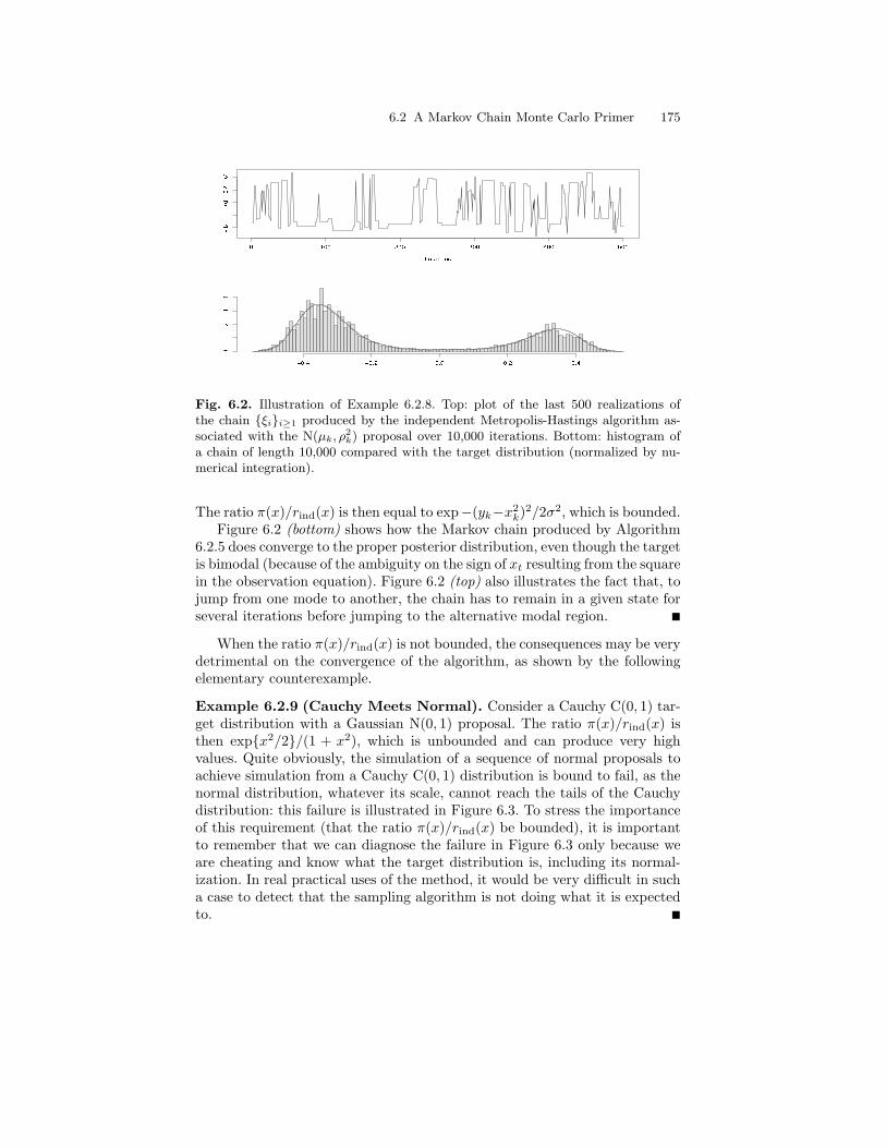
6.2 A Markov Chain Monte Carlo Primer 175

Fig. 6.2. Illustration of Example 6.2.8. Top: plot of the last 500 realizations ofthe chain ξii≥1 produced by the independent Metropolis-Hastings algorithm as-sociated with the N(µk, ρ

2k) proposal over 10,000 iterations. Bottom: histogram of

a chain of length 10,000 compared with the target distribution (normalized by nu-merical integration).

The ratio π(x)/rind(x) is then equal to exp−(yk−x2k)2/2σ2, which is bounded.

Figure 6.2 (bottom) shows how the Markov chain produced by Algorithm6.2.5 does converge to the proper posterior distribution, even though the targetis bimodal (because of the ambiguity on the sign of xt resulting from the squarein the observation equation). Figure 6.2 (top) also illustrates the fact that, tojump from one mode to another, the chain has to remain in a given state forseveral iterations before jumping to the alternative modal region.

When the ratio π(x)/rind(x) is not bounded, the consequences may be verydetrimental on the convergence of the algorithm, as shown by the followingelementary counterexample.

Example 6.2.9 (Cauchy Meets Normal). Consider a Cauchy C(0, 1) tar-get distribution with a Gaussian N(0, 1) proposal. The ratio π(x)/rind(x) isthen expx2/2/(1 + x2), which is unbounded and can produce very highvalues. Quite obviously, the simulation of a sequence of normal proposals toachieve simulation from a Cauchy C(0, 1) distribution is bound to fail, as thenormal distribution, whatever its scale, cannot reach the tails of the Cauchydistribution: this failure is illustrated in Figure 6.3. To stress the importanceof this requirement (that the ratio π(x)/rind(x) be bounded), it is importantto remember that we can diagnose the failure in Figure 6.3 only because weare cheating and know what the target distribution is, including its normal-ization. In real practical uses of the method, it would be very difficult in sucha case to detect that the sampling algorithm is not doing what it is expectedto.

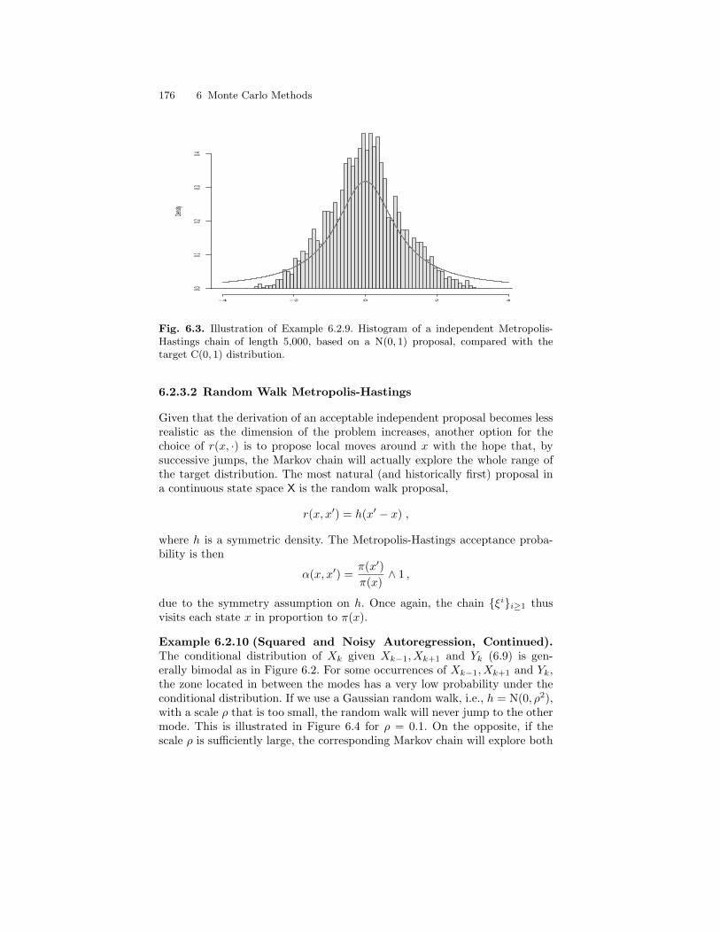
176 6 Monte Carlo Methods

Density

−4 −2 0 2 4

0.00.1

0.20.3

0.4

Fig. 6.3. Illustration of Example 6.2.9. Histogram of a independent Metropolis-Hastings chain of length 5,000, based on a N(0, 1) proposal, compared with thetarget C(0, 1) distribution.

6.2.3.2 Random Walk Metropolis-Hastings

Given that the derivation of an acceptable independent proposal becomes lessrealistic as the dimension of the problem increases, another option for thechoice of r(x, ·) is to propose local moves around x with the hope that, bysuccessive jumps, the Markov chain will actually explore the whole range ofthe target distribution. The most natural (and historically first) proposal ina continuous state space X is the random walk proposal,

r(x, x′) = h(x′ − x) ,

where h is a symmetric density. The Metropolis-Hastings acceptance proba-bility is then

α(x, x′) =π(x′)π(x)

∧ 1 ,

due to the symmetry assumption on h. Once again, the chain ξii≥1 thusvisits each state x in proportion to π(x).

Example 6.2.10 (Squared and Noisy Autoregression, Continued).The conditional distribution of Xk given Xk−1, Xk+1 and Yk (6.9) is gen-erally bimodal as in Figure 6.2. For some occurrences of Xk−1, Xk+1 and Yk,the zone located in between the modes has a very low probability under theconditional distribution. If we use a Gaussian random walk, i.e., h = N(0, ρ2),with a scale ρ that is too small, the random walk will never jump to the othermode. This is illustrated in Figure 6.4 for ρ = 0.1. On the opposite, if thescale ρ is sufficiently large, the corresponding Markov chain will explore both

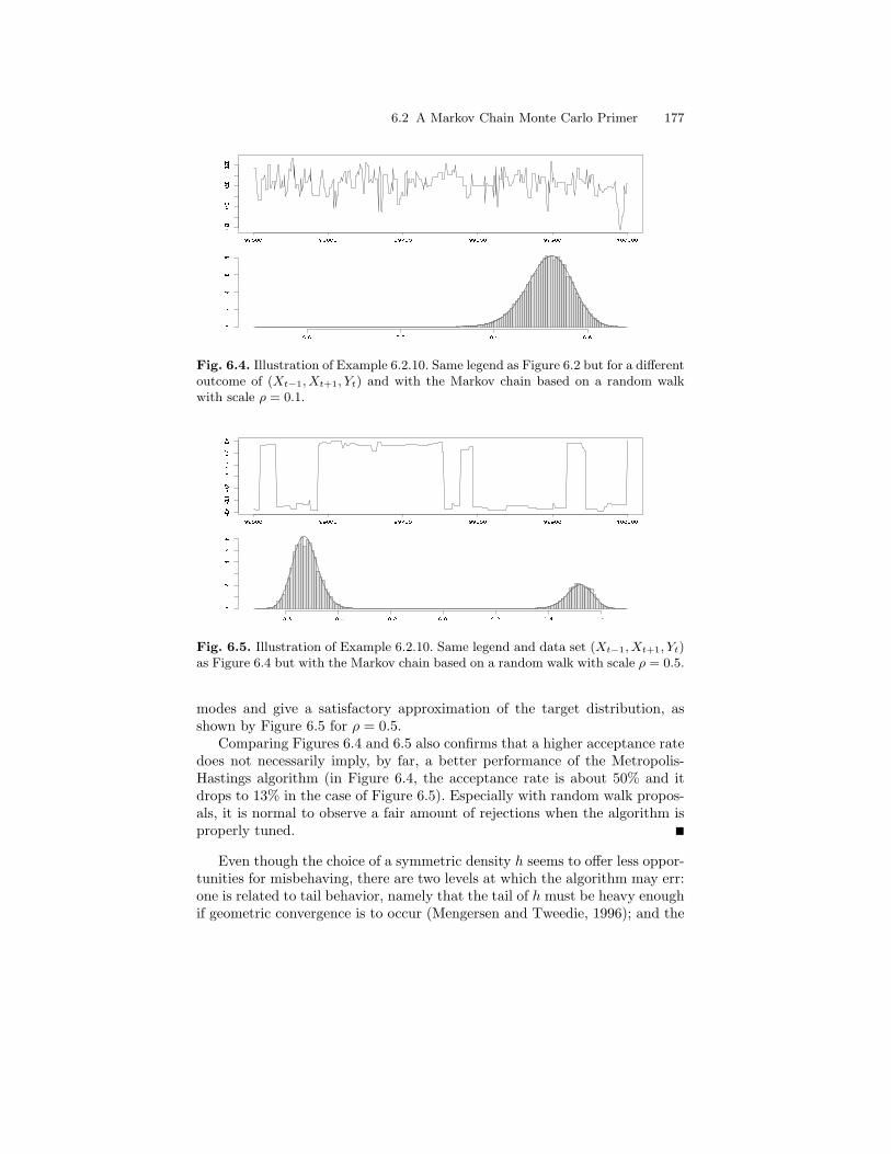
6.2 A Markov Chain Monte Carlo Primer 177

Fig. 6.4. Illustration of Example 6.2.10. Same legend as Figure 6.2 but for a differentoutcome of (Xt−1, Xt+1, Yt) and with the Markov chain based on a random walkwith scale ρ = 0.1.

Fig. 6.5. Illustration of Example 6.2.10. Same legend and data set (Xt−1, Xt+1, Yt)as Figure 6.4 but with the Markov chain based on a random walk with scale ρ = 0.5.

modes and give a satisfactory approximation of the target distribution, asshown by Figure 6.5 for ρ = 0.5.

Comparing Figures 6.4 and 6.5 also confirms that a higher acceptance ratedoes not necessarily imply, by far, a better performance of the Metropolis-Hastings algorithm (in Figure 6.4, the acceptance rate is about 50% and itdrops to 13% in the case of Figure 6.5). Especially with random walk propos-als, it is normal to observe a fair amount of rejections when the algorithm isproperly tuned.

Even though the choice of a symmetric density h seems to offer less oppor-tunities for misbehaving, there are two levels at which the algorithm may err:one is related to tail behavior, namely that the tail of h must be heavy enoughif geometric convergence is to occur (Mengersen and Tweedie, 1996); and the

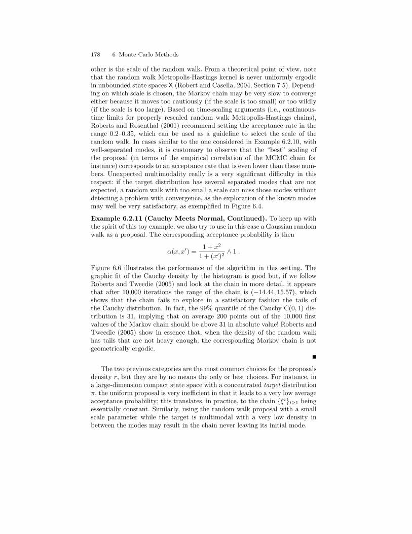
178 6 Monte Carlo Methods

other is the scale of the random walk. From a theoretical point of view, notethat the random walk Metropolis-Hastings kernel is never uniformly ergodicin unbounded state spaces X (Robert and Casella, 2004, Section 7.5). Depend-ing on which scale is chosen, the Markov chain may be very slow to convergeeither because it moves too cautiously (if the scale is too small) or too wildly(if the scale is too large). Based on time-scaling arguments (i.e., continuous-time limits for properly rescaled random walk Metropolis-Hastings chains),Roberts and Rosenthal (2001) recommend setting the acceptance rate in therange 0.2–0.35, which can be used as a guideline to select the scale of therandom walk. In cases similar to the one considered in Example 6.2.10, withwell-separated modes, it is customary to observe that the “best” scaling ofthe proposal (in terms of the empirical correlation of the MCMC chain forinstance) corresponds to an acceptance rate that is even lower than these num-bers. Unexpected multimodality really is a very significant difficulty in thisrespect: if the target distribution has several separated modes that are notexpected, a random walk with too small a scale can miss those modes withoutdetecting a problem with convergence, as the exploration of the known modesmay well be very satisfactory, as exemplified in Figure 6.4.

Example 6.2.11 (Cauchy Meets Normal, Continued). To keep up withthe spirit of this toy example, we also try to use in this case a Gaussian randomwalk as a proposal. The corresponding acceptance probability is then

α(x, x′) =1 + x2

1 + (x′)2∧ 1 .

Figure 6.6 illustrates the performance of the algorithm in this setting. Thegraphic fit of the Cauchy density by the histogram is good but, if we followRoberts and Tweedie (2005) and look at the chain in more detail, it appearsthat after 10,000 iterations the range of the chain is (−14.44, 15.57), whichshows that the chain fails to explore in a satisfactory fashion the tails ofthe Cauchy distribution. In fact, the 99% quantile of the Cauchy C(0, 1) dis-tribution is 31, implying that on average 200 points out of the 10,000 firstvalues of the Markov chain should be above 31 in absolute value! Roberts andTweedie (2005) show in essence that, when the density of the random walkhas tails that are not heavy enough, the corresponding Markov chain is notgeometrically ergodic.

The two previous categories are the most common choices for the proposalsdensity r, but they are by no means the only or best choices. For instance, ina large-dimension compact state space with a concentrated target distributionπ, the uniform proposal is very inefficient in that it leads to a very low averageacceptance probability; this translates, in practice, to the chain ξii≥1 beingessentially constant. Similarly, using the random walk proposal with a smallscale parameter while the target is multimodal with a very low density inbetween the modes may result in the chain never leaving its initial mode.

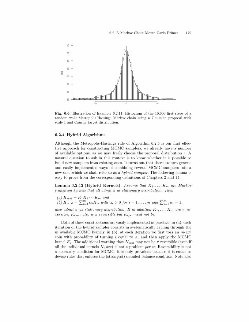
6.2 A Markov Chain Monte Carlo Primer 179

Density

−5 0 5

0.000.05

0.100.15

0.200.25

0.300.35

Fig. 6.6. Illustration of Example 6.2.11. Histogram of the 10,000 first steps of arandom walk Metropolis-Hastings Markov chain using a Gaussian proposal withscale 1 and Cauchy target distribution.

6.2.4 Hybrid Algorithms

Although the Metropolis-Hastings rule of Algorithm 6.2.5 is our first effec-tive approach for constructing MCMC samplers, we already have a numberof available options, as we may freely choose the proposal distribution r. Anatural question to ask in this context is to know whether it is possible tobuild new samplers from existing ones. It turns out that there are two genericand easily implemented ways of combining several MCMC samplers into anew one, which we shall refer to as a hybrid sampler. The following lemma iseasy to prove from the corresponding definitions of Chapters 2 and 14.

Lemma 6.2.12 (Hybrid Kernels). Assume that K1, . . . ,Km are Markovtransition kernels that all admit π as stationary distribution. Then

(a) Ksyst = K1K2 · · ·Km and(b) Krand =

∑mi=1 αiKi, with αi > 0 for i = 1, . . . ,m and

∑mi=1 αi = 1,

also admit π as stationary distribution. If in addition K1, . . . ,Km are π re-versible, Krand also is π reversible but Ksyst need not be.

Both of these constructions are easily implemented in practice: in (a), eachiteration of the hybrid sampler consists in systematically cycling through them available MCMC kernels; in (b), at each iteration we first toss an m-arycoin with probability of turning i equal to αi and then apply the MCMCkernel Ki. The additional warning that Ksyst may not be π reversible (even ifall the individual kernels Ki are) is not a problem per se. Reversibility is nota necessary condition for MCMC, it is only prevalent because it is easier todevise rules that enforce the (strongest) detailed balance condition. Note also

180 6 Monte Carlo Methods

that it is always possible to induce reversibility by appropriate modificationsof the cycling strategy. For instance, the symmetric combination KsystKrev

with Krev = KmKm−1 · · ·K1 is easily checked to be π reversible. In practice,it means that the cycle through the various available MCMC kernels Ki hasto be done in descending and then ascending order.

Regarding irreducibility, it is clear that the random scan kernel Krand

is guaranteed to be phi-irreducible if at least one of the kernels Ki is. Forthe systematic scan strategy, the situation is more complex and Ksyst mayfail to be phi-irreducible even in cases where all the individual kernels Ki

are phi-irreducible (with common irreducibility measure φ). A more usefulremark is that if K1, . . . ,Km all admit π as stationary distribution but are notphi-irreducible—meaning that they do not yet correspond to fully functionalconverging MCMC algorithms—there are cases where both Ksyst and Krand

are phi-irreducible. It is thus possible to build viable sampling strategies fromindividual MCMC transitions that are not in themselves fully functional. Themain application of this remark is to break large-dimensional problems intosmaller ones by modifying only one part of the state at a time.

6.2.5 Gibbs Sampling

When the distribution of interest is multivariate, it may be the case thatfor each particular variable, its conditional distribution given all remainingvariables has a simple form. This is in particular the case for models specifiedusing conditional independence relations like HMMs and more general latentvariable models. In this case, a natural MCMC algorithm is the so-called Gibbssampler, which we now describe. Its name somehow inappropriately stemsfrom its use for the simulation of Gibbs Markov random fields by Geman andGeman (1984).

6.2.5.1 A Generic Conditional Algorithm

Suppose we are given a joint distribution with probability density functionπ on a space X such that x ∈ X may be decomposed into m componentsx = (x1, . . . , xm), where xk ∈ Xk. If k is an index in 1, . . . ,m, we shalldenote by xk the kth component of x and by x−k = xll 6=k the collectionof remaining components. We further denote by πk(·|x−k) the conditionalprobability density function of Xk given Xll 6=k and assume that simulationfrom this conditional distribution is feasible (for k = 1, . . . ,m). Note that xkis not necessarily scalar but may be itself vector-valued.

Algorithm 6.2.13 (Gibbs Sampler). Starting from an initial arbitrary stateξ1, update the current state ξi = (ξi1, . . . , ξ

im) to a new state ξi+1 as follows.

For k = 1, 2, . . . ,m: Simulate ξi+1k from πi(·|ξi+1

1 , . . . , ξi+1k−1, ξ

ik+1, . . . , ξ

im).

6.2 A Markov Chain Monte Carlo Primer 181

In other words, in the kth round of the cycle needed to simulate ξi+1,the kth component is updated by simulation from its conditional distributiongiven all other components (which remain fixed). This new value then super-sedes the old one and is used in the subsequent simulation steps. A completeround of m conditional simulations is usually referred to as a sweep of thealgorithm. Another representation of the Gibbs sampler is to break the com-plete cycle as a combination of m individual MCMC steps where only one ofthe m components is modified according to the corresponding conditional dis-tribution. This approach is easily recognized as the combination of type (a)—systematic cycling—in Lemma 6.2.12. Hence we know from Lemma 6.2.12that the correct behavior of the complete cycle can be inferred from that ofthe individual updates. The next result is a first step in this direction.

Proposition 6.2.14 (Reversibility of Individual Gibbs Steps). Each ofthe m individual steps of the Gibbs sampler (Algorithm 6.2.13) is π reversibleand thus admits π as a stationary probability density function.

Proof. Consider the step that updates the kth component and denote by Kk

the corresponding transition kernel. We can always write λ = λk⊗λ−k whereλk and λ−k are measures on Xk and X−k, respectively, such that λk dominatesπk(·|x−k) for all values of xk ∈ Xk. With these notations,

Kk(x, dx′) = δx−k(dx′−k)πk(x′k|x−k)λk(dx′k) .

Hence, for any functions f1, f2 ∈ Fb (X),∫∫f1(x)f2(x′)π(x)λ(dx)K(x, dx′) =∫ f1(x)π(x)λk(dxk)

∫f2(x′k, x−k)πk(x′k|x−k)λk(dx′k)

λ−k(dx−k) ,

where (x′k, x−k) refers to the element u of X such that uk = x′k and u−k = x−k.Because π(xk, x−k)πk(x′k|x−k) = πk(xk|x−k)π(x′k, x−k), we may also write∫∫

f1(x)f2(x′)π(x)λ(dx)K(x, dx′) =∫ f2(x′k, x−k)π(x′k, x−k)λk(dx′k)

×∫f1(xk, x−k)πk(xk|x−k)λk(dxk)

λ−k(dx−k) ,

which is the same expression as before where the roles of f1 and f2 have beenexchanged, thus showing that the detailed balance condition (2.12) holds. ut

An insightful interpretation of Proposition 6.2.14 is that each step corre-sponds to a very special type of Metropolis-Hastings move where the accep-tance probability is uniformly equal to 1, due to choice of πk as the proposal

182 6 Monte Carlo Methods

distribution. However, Proposition 6.2.14 does not suffice to establish properconvergence of the Gibbs sampler, as none of the individual steps produces aphi-irreducible chain. Only the combination of the m moves in the completecycle has a chance of producing a chain with the ability to visit the wholespace X from any starting point. Of course, one can also adopt the combina-tion of type (b) in Lemma 6.2.12 to obtain the random scan Gibbs sampler asopposed to the systematic scan Gibbs sampler, which corresponds to the solu-tion exposed in Algorithm 6.2.13. We refer to (Robert and Casella, 2004) and(Roberts and Tweedie, 2005) for more precise convergence results pertainingto these variants of the Gibbs sampler.

One perspective that is somehow unique to Gibbs sampling is Rao-Blackwellization, named after the Rao-Blackwell theorem used in classicalstatistics (Lehmann and Casella, 1998) and recalled as Proposition A.2.5. Itis in essence a variance reduction technique (see Robert and Casella, 2004,Chapter 4) that takes advantage of the conditioning abilities of the Gibbssampler. If only a part of the vector x is of interest (as is often the case inlatent variable models), say xk, Rao-Blackwellization consists in replacing theempirical average

πMCMCN (f) =

1N

N∑i=1

f(ξik) with πRBN (f) =

1N

N∑i=1

Eπ[f(ξk) | ξi−k] ,

where ξii≥1 denotes the chain produced by Algorithm 6.2.13. This is ofcourse only feasible in cases where the integral of the function of interestf under πk(·|x−k) may be easily evaluated for all x ∈ X. In i.i.d. settings,πMCMCN (f) would be more variable than πRB

N (f) by Proposition A.2.5. ForMarkov chain simulations ξii≥1, this is not necessarily the case, and it isonly in specific situations (see Robert and Casella, 2004, Sections 9.3 and10.4.3) that the latter estimate can be shown to be less variable. Anothersubstantial benefit of Rao-Blackwellization is to provide an elegant method forthe approximation of probability density functions of the different componentsof x. Indeed,

1N

N∑i=1

πk(·∣∣ξi−k )

is unbiased and converges to the marginal density of kth component, underthe target distribution. If the conditional probability density functions areavailable in closed form, it is unnecessary (and inefficient) to use nonparamet-ric density estimation methods such as kernel methods for postprocessing theoutput of Gibbs sampling.

We now discuss a clever use of the Gibbs sampling principle, known as theslice sampler, which is of interest in its own right.

6.2 A Markov Chain Monte Carlo Primer 183

6.2.5.2 The Slice Sampler

Proposition 6.2.2 asserts that the bivariate random variable (X,U) whosedistribution is uniform on

Sπ =

(x, u) ∈ X× R+ : 0 ≤ u ≤ π(x),

is such that the marginal distribution of X is π. This observation is at thecore of the accept-reject algorithm discussed in Section 6.2.1. We will usethe letter U to denote uniform distributions on sets, writing, for instance,(X,U) ∼ U (Sπ).

From the perspective of MCMC algorithms, we can consider using a ran-dom walk on Sπ to produce a Markov chain with stationary distribution equalto this uniform distribution on Sπ. There are many ways of implementing arandom walk on this set, but a natural solution is to go one direction at atime, that is, to move iteratively along the u-axis and then along the x-axis.Furthermore, we can use uniform moves in both directions; that is, startingfrom a point (x, u) in Sπ, the move along the u-axis will correspond to theconditional distribution

U (u : u ≤ π(ξ)) , (6.10)

resulting in a change from point (x, u) to point (x, u′), still in Sπ, and thenthe move along the ξ-axis to the conditional distribution

U (x : π(x) ≥ u′) , (6.11)

resulting in a change from point (x, u′) to point (x′, u′). This set of proposalsis the basis chosen for the original slice sampler of Damien and Walker (1996),Neal (1997) (published as Neal, 2003), and Damien et al. (1999).

Algorithm 6.2.15 (Slice Sampler). Starting from an arbitrary point (ξ1, U1)in Sπ, simulate for i ≥ 1,

1. U i+1 ∼ U([0, π(ξi)]

);

2. ξi+1 ∼ U(S(U i+1)

), with S(u) = x : π(x) ≥ u.

The important point here is that Algorithm 6.2.15 is validated as a Gibbssampling method, as steps 1 and 2 in the above are simply the conditionaldistributions of U and ξ associated with the joint distribution U (Sπ).

Obviously, this does not make the slice sampler a universal generator:in many settings, resolving the simulation from the uniform U (S(u)) is justas hard (and impossible) as to generate directly from π, and extensions areoften necessary (Robert and Casella, 2004, Chapter 8). Still, this potentialuniversality shows that Gibbs sampling does not only pertain to a specialcategory of hierarchical models.

Example 6.2.16 (Single Site Conditional Distribution in StochasticVolatility Model). To illustrate the slice sampler, we consider the stochastic

184 6 Monte Carlo Methods

volatility model discussed in Example 1.3.13 whose state-space form is asfollows:

Xk+1 = φXk + σUk ,

Yk = β exp(Xk/2)Vk ,

where Ukk≥0 and Vkk≥0 are independent standard Gaussian white noiseprocesses. In this model, β2 exp(Xk) is referred to as the volatility, and itsestimation is one of the purposes of the analysis (see Example 1.3.13 fordetails). As in Example 6.2.8 above, we consider the conditional distribution ofXk givenXk−1, Xk+1 and Yk, whose transition density function πk(x|xk−1, xk)is proportional to

exp[−

(xk+1 − φx)2

2σ2+

(x− φxk−1)2

2σ2

]1

β exp(x/2)exp

[− y2

k

2β2 exp(x)

],

(6.12)ignoring constants. In fact, terms that do not depend on x can be ignored aswell, and we may complete the square (in x) to obtain

πk(x|xk−1, xk) ∝ exp[−1 + φ2

2σ2

(x− µk)2 +

y2kσ

2

(1 + φ2)β2exp(−x)

],

where

µk =φ(xk+1 + xk−1)− σ2/2

1 + φ2. (6.13)

Defining

αk =y2kσ

2 exp(−µk)(1 + φ2)β2

and ρ =1 + φ2

2σ2, (6.14)

πk(x|xk−1, xk) is thus proportional to

exp[−ρ

(x− µk)2 + αk exp[−(x− µk)]]

.

The parameter µk corresponds to a simple shift that poses no simulation prob-lem. Hence, the general form of the conditional probability density functionfrom which simulation is required is exp[−ρx2 +α exp(−x)] for positive val-ues of ρ and α. Shephard and Pitt (1997) (among others) discuss an approachbased on accept-reject ideas for carrying out this conditional simulation, butwe may also use the slice sampler for this purpose. The second step of Al-gorithm 6.2.15 then requires simulation from the uniform distribution on theset

S(u) =x : exp[−ρx2 + α exp(−x)] ≥ u

=x : x2 + α exp(−x) ≤ ω

,

setting ω = −(1/ρ) log u. Now, while the inversion of x2 + α exp(−x) = ω isnot possible analytically, the fact that this function is convex (for α > 0) andthat the previous value of x belongs to the set S(u) help in solving this equa-tion by numerical trial-and-error or more elaborate zero-finding algorithms.

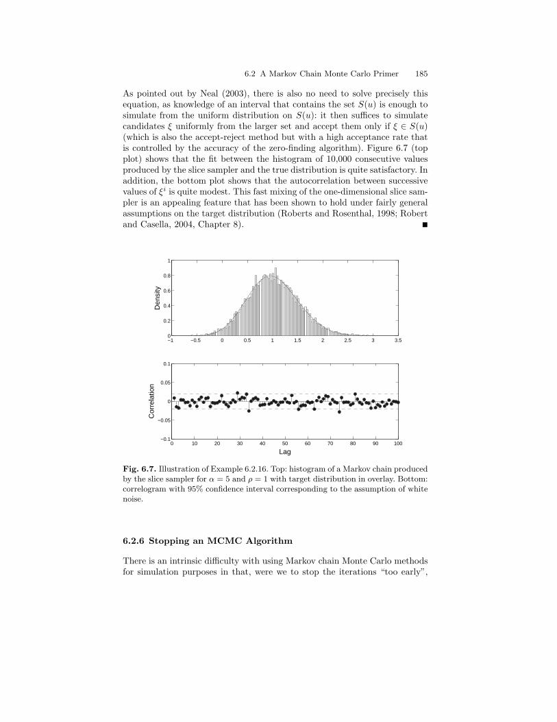
6.2 A Markov Chain Monte Carlo Primer 185

As pointed out by Neal (2003), there is also no need to solve precisely thisequation, as knowledge of an interval that contains the set S(u) is enough tosimulate from the uniform distribution on S(u): it then suffices to simulatecandidates ξ uniformly from the larger set and accept them only if ξ ∈ S(u)(which is also the accept-reject method but with a high acceptance rate thatis controlled by the accuracy of the zero-finding algorithm). Figure 6.7 (topplot) shows that the fit between the histogram of 10,000 consecutive valuesproduced by the slice sampler and the true distribution is quite satisfactory. Inaddition, the bottom plot shows that the autocorrelation between successivevalues of ξi is quite modest. This fast mixing of the one-dimensional slice sam-pler is an appealing feature that has been shown to hold under fairly generalassumptions on the target distribution (Roberts and Rosenthal, 1998; Robertand Casella, 2004, Chapter 8).

0 10 20 30 40 50 60 70 80 90 100−0.1

−0.05

0

0.05

0.1

Lag

Cor

rela

tion

−1 −0.5 0 0.5 1 1.5 2 2.5 3 3.50

0.2

0.4

0.6

0.8

1

Den

sity

Fig. 6.7. Illustration of Example 6.2.16. Top: histogram of a Markov chain producedby the slice sampler for α = 5 and ρ = 1 with target distribution in overlay. Bottom:correlogram with 95% confidence interval corresponding to the assumption of whitenoise.

6.2.6 Stopping an MCMC Algorithm

There is an intrinsic difficulty with using Markov chain Monte Carlo methodsfor simulation purposes in that, were we to stop the iterations “too early”,

186 6 Monte Carlo Methods

we would still be influenced by the (arbitrary) starting value of the chain,and were we to stop the iteration “too late”, we would be wasting simula-tion time. In contrast with what happens for independent Monte Carlo where(6.1) may be used to obtain confidence intervals, it is fairly difficult to esti-mate the accuracy of estimates derived from the MCMC sample because ofthe unknown correlation structure of the simulated ξi. Apart for often usefulgraphic diagnostics (trace of the samples, correlograms, comparison of his-tograms obtained with different starting points...), there exist (more or less)empirical rules that provide hints on when an MCMC sampler should bestopped. A branch of MCMC, known as perfect sampling, corresponds to arefinement of these rules in which the aim is to guarantee that the Markovchain, when observed at appropriate times, is exactly distributed from thestationary distribution. Not surprisingly, these methods are very difficult todevise and equally costly to implement. Another direction, generally referredto as computable bounds, consists in obtaining bounds on the convergencespeed of MCMC-generated Markov chains. When available, such results arevery powerful, as they do not require any empirical estimation, and the num-ber of required MCMC simulations may be calibrated beforehand. Of course,the drawback here is that for complex samplers, typically hybrid samplers thatincorporate several different MCMC sampling steps, such results are simplynot available (Robert and Casella, 2004).

6.3 Applications to Hidden Markov Models

This section describes methods that may be used to simulate the unobservablesequence of states X0:n given the corresponding observations Y0:n in HMMs forwhich the direct (independent) Monte Carlo simulations methods discussedin Section 6.1.2 are not applicable.

We start from the most generic and easily implementable approaches inwhich each individual hidden state Xk is simulated conditionally on all Xl

except itself. We then move to a more specific sampling technique that takesprofit of the structure found in conditionally Gaussian linear state-space mod-els (see, in particular, Definition 2.2.6 and Sections 4.2.3 and 5.2.6).

6.3.1 Generic Sampling Strategies

6.3.1.1 Single Site Sampling

We now formalize an argument that was underlying in Examples 6.2.8and 6.2.16. Starting from the joint conditional distribution of X0:n given Y0:n

defined (up to a proportionality constant) by (6.7), the conditional probabilitydensity function of a single variable in the hidden chain, Xk say, given Y0:n

and its two neighbors Xk−1 and Xk+1 is such that

6.3 Applications to Hidden Markov Models 187

φk−1:k+1|n(xk|xk−1, xk+1) ∝ φk−1:k+1|n(xk−1, xk, xk+1)∝ q(xk−1, xk)q(xk, xk+1)gk(xk) . (6.15)

At the two endpoints k = 0 and k = n, we have the obvious corrections

φ0:1|n(x0|x1) ∝ ν(x0)q(x0, x1)

andφn−1:n|n(xn|xn−1) ∝ q(xn−1, xn)gn(xn) .

Therefore, if we aim at simulating the whole vector X0:n by the most ba-sic Gibbs sampler that simulates one component of the vector at a time,φk−1:k+1|n(xk|xk−1, xk+1) is given by (6.15) in a simple closed-form expres-sion. Remember that the expression looks simple only because knowledge ofthe normalization factor is not required for performing MCMC simulations.

In the case where X is finite, the simulation of X0:n by this Gibbs samplingapproach is rather straightforward, as the only operations that are requested(for k = 0, . . . , n) are

• computing q(xk−1, x)q(x, xk+1)gk(x) for all values of x ∈ X and normaliz-ing them to form a probability vector πk;

• simulating a value of the state according to πk.

It is interesting to contrast this Gibbs sampling algorithm with the simplerMonte Carlo approach of Algorithm 6.1.1. A complete sweep of the Gibbssampler is simpler to implement, as each Gibbs simulation step requires thatr products be computed (where r is the cardinality of X). Hence, the completeGibbs sweep requires O (r(n+ 1)) operations compared to O

(r2(n+ 1)

)for

Algorithm 6.1.1 due to the necessity of computing all the filtering distribu-tions by Algorithm 5.1.1. On the other hand, the Monte Carlo simulationsobtained by Algorithm 6.1.1 are independent, which is not the case for thoseproduced by Gibbs sampling. For a comparable computational effort, we maythus perform r times as many simulations by Gibbs sampling than by inde-pendent Monte Carlo. This does not necessarily correspond to a gain though,as the variance of MCMC estimates is most often larger than that of MonteCarlo ones due to the Markov dependence between successive samples. It re-mains that if the number of possible values of Xk is very large (a case usuallyfound in related models used in applications such as image processing), it maybe the case that implementing Monte Carlo simulation is overwhelming whilethe Gibbs sampler is still feasible.

It is generally true that, apart from this case (finite but very large statespace), there are very few examples of hidden Markov models where theGibbs sampling approach is applicable and the general Monte Carlo ap-proach of Section 6.1.2.1 is not. This has to do with the fact that determiningφk−1:k+1|n(·|xk−1, xk+1) exactly, not only up to a constant, involves exactlythe same type of marginalization operation involved in the implementation

188 6 Monte Carlo Methods

of the filtering recursion. An important point to stress here is that replac-ing an exact simulation by a Metropolis-Hastings step in a general MCMCalgorithm does not jeopardize its validity as long as the Metropolis-Hastingsstep is associated with the correct stationary distribution. Hence, the mostnatural alternative to the Gibbs sampler in cases where sampling from the fullconditional distribution is not directly feasible is the one-at-a-time Metropolis-Hastings algorithm that combines successive Metropolis-Hastings steps thatupdate only one of the variables. For k = 0, . . . , n, we thus update the kthcomponent xik of the current simulated sequence of states xi by proposing anew candidate for xi+1

k and accepting it according to (6.5), using (6.15) as thetarget.

Example 6.3.1 (Single Site Conditional Distribution in StochasticVolatility Model, Continued). We return to the stochastic volatility modelalready examined in Example 6.2.16 but with the aim of simulating completesequences under the posterior distribution rather than just individual states.From the preceding discussion, we may use the algorithm described in Exam-ple 6.2.16 for each index (k = 0, . . . , n) in the sequence of states to simulate.Although the algorithm itself applies to all indices, the expression of µk, αkand ρ in (6.13)–(6.14) need to be modified for the two endpoints as follows.

For k = 0, the first term in (6.12) should be replaced by

exp−

(x1 − φx)2

2σ2+

(1− φ2)x2

2σ2

, (6.16)

as it is sensible to assume that the initial state X0 is a priori distributed asthe stationary distribution of the AR(1) process, that is, N

(0, σ2/(1− φ2)

).

Hence for k = 0, (6.13) and (6.14) should be replaced byµ0 = φx1 − σ2/2 ,α0 = Y 2

0 σ2 exp(−µ0)/β2 ,

ρ0 = 1/(2σ2) .(6.17)

For k = n, the first term in (6.12) reduces to

exp−

(x− xn−1)2

2σ2

, (6.18)

and thus µn = φxn−1 − σ2/2 ,αn = Y 2

n σ2 exp(−µn)/β2 ,

ρn = 1/(2σ2) ,(6.19)

replace (6.13) and (6.14).An iteration of the complete algorithm thus proceeds by computing, for

each index k = 0, . . . , n in turn, µk, αk and ρ according to (6.13) and (6.14),or (6.17) or (6.19) if k = 0 or n. Then one iteration of the slice samplingalgorithm discussed in Example 6.2.16 is applied.

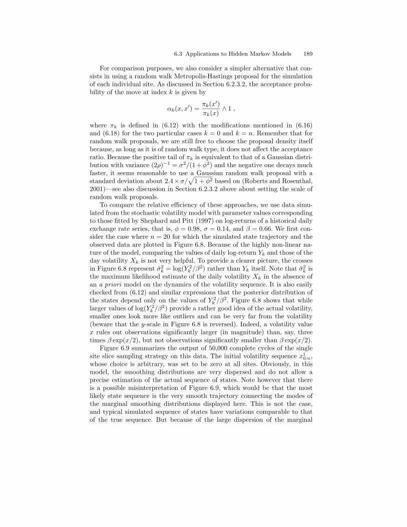
6.3 Applications to Hidden Markov Models 189

For comparison purposes, we also consider a simpler alternative that con-sists in using a random walk Metropolis-Hastings proposal for the simulationof each individual site. As discussed in Section 6.2.3.2, the acceptance proba-bility of the move at index k is given by

αk(x, x′) =πk(x′)πk(x)

∧ 1 ,

where πk is defined in (6.12) with the modifications mentioned in (6.16)and (6.18) for the two particular cases k = 0 and k = n. Remember that forrandom walk proposals, we are still free to choose the proposal density itselfbecause, as long as it is of random walk type, it does not affect the acceptanceratio. Because the positive tail of πk is equivalent to that of a Gaussian distri-bution with variance (2ρ)−1 = σ2/(1 +φ2) and the negative one decays muchfaster, it seems reasonable to use a Gaussian random walk proposal with astandard deviation about 2.4×σ/

√1 + φ2 based on (Roberts and Rosenthal,

2001)—see also discussion in Section 6.2.3.2 above about setting the scale ofrandom walk proposals.

To compare the relative efficiency of these approaches, we use data simu-lated from the stochastic volatility model with parameter values correspondingto those fitted by Shephard and Pitt (1997) on log-returns of a historical dailyexchange rate series, that is, φ = 0.98, σ = 0.14, and β = 0.66. We first con-sider the case where n = 20 for which the simulated state trajectory and theobserved data are plotted in Figure 6.8. Because of the highly non-linear na-ture of the model, comparing the values of daily log-return Yk and those of theday volatility Xk is not very helpful. To provide a clearer picture, the crossesin Figure 6.8 represent σ2

k = log(Y 2k /β

2) rather than Yk itself. Note that σ2k is

the maximum likelihood estimate of the daily volatility Xk in the absence ofan a priori model on the dynamics of the volatility sequence. It is also easilychecked from (6.12) and similar expressions that the posterior distribution ofthe states depend only on the values of Y 2

k /β2. Figure 6.8 shows that while

larger values of log(Y 2k /β

2) provide a rather good idea of the actual volatility,smaller ones look more like outliers and can be very far from the volatility(beware that the y-scale in Figure 6.8 is reversed). Indeed, a volatility valuex rules out observations significantly larger (in magnitude) than, say, threetimes β exp(x/2), but not observations significantly smaller than β exp(x/2).

Figure 6.9 summarizes the output of 50,000 complete cycles of the singlesite slice sampling strategy on this data. The initial volatility sequence x1

0:n,whose choice is arbitrary, was set to be zero at all sites. Obviously, in thismodel, the smoothing distributions are very dispersed and do not allow aprecise estimation of the actual sequence of states. Note however that thereis a possible misinterpretation of Figure 6.9, which would be that the mostlikely state sequence is the very smooth trajectory connecting the modes ofthe marginal smoothing distributions displayed here. This is not the case,and typical simulated sequence of states have variations comparable to thatof the true sequence. But because of the large dispersion of the marginal

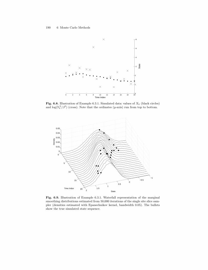
190 6 Monte Carlo Methods

0 2 4 6 8 10 12 14 16 18 20

−8

−6

−4

−2

0

2

4

Sta

te

Time Index

Fig. 6.8. Illustration of Example 6.3.1. Simulated data: values of Xk (black circles)and log(Y 2

k /β2) (cross). Note that the ordinates (y-axis) run from top to bottom.

−1−0.5

00.5

11.5

2

0

5

10

15

20

0

0.01

0.02

0.03

0.04

0.05

State

Time Index

Den

sity

Fig. 6.9. Illustration of Example 6.3.1. Waterfall representation of the marginalsmoothing distributions estimated from 50,000 iterations of the single site slice sam-pler (densities estimated with Epanechnikov kernel, bandwidth 0.05). The bulletsshow the true simulated state sequence.

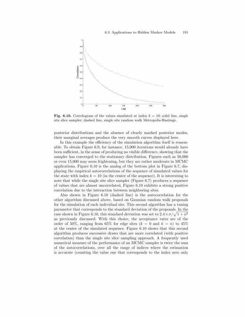
6.3 Applications to Hidden Markov Models 191

Slice SamplerRandom Walk M−H

0 50 100 150 200 250 3000

0.1

0.2

0.3

0.4

0.5

0.6

0.7

0.8

0.9

1

Lag

Cor

rela

tion

Fig. 6.10. Correlogram of the values simulated at index k = 10: solid line, singlesite slice sampler; dashed line, single site random walk Metropolis-Hastings.

posterior distributions and the absence of clearly marked posterior modes,their marginal averages produce the very smooth curves displayed here.

In this example the efficiency of the simulation algorithm itself is reason-able. To obtain Figure 6.9, for instance, 15,000 iterations would already havebeen sufficient, in the sense of producing no visible difference, showing that thesampler has converged to the stationary distribution. Figures such as 50,000or even 15,000 may seem frightening, but they are rather moderate in MCMCapplications. Figure 6.10 is the analog of the bottom plot in Figure 6.7, dis-playing the empirical autocorrelations of the sequence of simulated values forthe state with index k = 10 (in the center of the sequence). It is interesting tonote that while the single site slice sampler (Figure 6.7) produces a sequenceof values that are almost uncorrelated, Figure 6.10 exhibits a strong positivecorrelation due to the interaction between neighboring sites.

Also shown in Figure 6.10 (dashed line) is the autocorrelation for theother algorithm discussed above, based on Gaussian random walk proposalsfor the simulation of each individual site. This second algorithm has a tuningparameter that corresponds to the standard deviation of the proposals. In thecase shown in Figure 6.10, this standard deviation was set to 2.4×σ/

√1 + φ2

as previously discussed. With this choice, the acceptance rates are of theorder of 50%, ranging from 65% for edge sites (k = 0 and k = n) to 45%at the center of the simulated sequence. Figure 6.10 shows that this secondalgorithm produces successive draws that are more correlated (with positivecorrelation) than the single site slice sampling approach. A frequently usednumerical measure of the performance of an MCMC sampler is twice the sumof the autocorrelations, over all the range of indices where the estimationis accurate (counting the value one that corresponds to the index zero only

192 6 Monte Carlo Methods

once). This number is equal to the ratio of the asymptotic variance of thesample mean of the simulated values, say 1/N

∑Ni=1 x

i10 in our case, to the

corresponding Monte Carlo variance for independent simulations under thetarget distribution (Meyn and Tweedie, 1993, Theorem 17.5.3; Robert andCasella, 2004, Theorem 6.65). Thus this ratio, which is sometimes referred toas the integrated autocorrelation time, may be interpreted as the price to pay(in terms of extra simulations) for using correlated draws. For the approachbased on slice sampling this factor is equal to 120, whereas it is about 440when using random walk proposals. Hence the method based on random walkis about four times less efficient, or more appropriately requires about fourtimes as many iterations to obtain comparable results in terms of variance ofthe estimates. Note that this measure should not be over-interpreted, as theasymptotic variance of estimates of the form 1/N

∑Ni=1 f(xi0:n) will obviously

depend on the function f as well. In addition, each iteration of the randomwalk sampler runs faster than for the sampler based on slice sampling.

It is important to understand that the performance of a sampler dependscrucially on the characteristics of the target distribution. More specifically,in our example it depends on the values of the parameters of the model, (σ,φ, β), but also on the particular observed sequence Y0:n under consideration.This is a serious concern in contexts such as those of Chapters 11 and 13,where it is required to simulate sequences of states under widely varying, andsometimes very unlikely, choices of the parameters. To illustrate this point, wereplaced Y10 by the value β exp(5/2), which corresponds to a rather significantpositive (and hence very informative) outlier in Figure 6.8. Figure 6.11 showsthe effect of this modification on the marginal smoothing distributions. Forthis particular data set, the integrated autocorrelation time at index k = 10increases only slightly (140 versus 120 above) for the sampler based on singlesite slice sampling but more significantly (450 versus 220) for the sampler thatuses random walk proposals.

In Figures 6.9 and 6.11, the length of the sequence to simulate was indeedquite short (n = 20). An important issue in many applications is to knowwhether or not the efficiency of the sampler will deteriorate significantly whenmoving to longer sequences. Loosely speaking the answer is “no, in general”for HMMs due to the forgetting properties of the posterior distribution. Whenthe conditions discussed in Section 4.3 hold, the posterior correlation betweendistant sites is indeed low and thus single site sampling does not really be-come worse as the overall length of the sequence increases. Figure 6.12 forinstance shows the results obtained for n = 200 with the same number ofMCMC iterations. For the slice sampling based approach, the integrated au-tocorrelation time at index k = 100 is about 90, that is, comparable to whatwas observed for the shorter observation sequence2 (see also Figure 8.6 andrelated comments for further discussion of this issue).

2It is indeed even slightly lower due to the fact that mixing is somewhat betterfar from the edges of the sequence to be simulated. The value measured at index

6.3 Applications to Hidden Markov Models 193

00.5

11.5

22.5

3

0

5

10

15

20

0

0.02

0.04

0.06

State

Time Index

Den

sity

Fig. 6.11. Same plot as Figure 6.9 where Y10 has been replaced by a positive outlier.

Sta

te

Time Index0 20 40 60 80 100 120 140 160 180 200

−1.5

−1

−0.5

0

0.5

1

1.5

Fig. 6.12. Illustration of Example 6.3.1. Grey level representation of the smoothingdistributions estimated from 50,000 iterations of the single site slice sampler (densi-ties estimated with Epanechnikov kernel, bandwidth 0.05). The bold line shows thetrue simulated state sequence.

194 6 Monte Carlo Methods

We conclude this example by noting that slice sampling is obviously notthe only available approach to tackle posterior simulation in this model andwe do not claim that it is necessary the best one either. Because of its practicalimportance in econometric applications, MCMC approaches suitable for thismodel have been considered by several authors including Jacquier et al. (1994),Shephard and Pitt (1997) and Kim et al. (1998).

6.3.1.2 Block Sampling Strategies

In some cases, single site updating can be painfully slow. It is thus of interest totry to speed up the simulation by breaking some of the dependence involved insingle site updating. A natural solution is to propose a joint update of a groupof Xk, as this induces more variability in the simulated values. This strategyhas been shown to be successful in some particular models (Liu et al., 1994).The drawback of this approach however is that when the size of the blocksincreases, it is sometimes difficult to imagine efficient proposal strategies inlarger dimensional spaces. For the stochastic volatility model discussed abovefor instance, Shephard and Pitt (1997) discuss the use of approximations basedon Gaussian expansions.

There are no general rules here, however, and the eventual improvementsin mixing speed have to be gauged at the light of the extra computationalefforts required to simulate larger blocks. In the case of multivariate Gaussiandistributions for instance, simulating in blocks of size m involves computingthe Cholevski factorization of m by m matrices, an operation whose cost is oforder m3. Hence moving to block simulations will be most valuable in caseswhere single site sampling is pathologically slow.

6.3.2 Gibbs Sampling in CGLSSMs

For the stochastic volatility model, Kim et al. (1998) (among others) advocatethe use of a specific technique that consists in approximating the behaviorof the model by a conditionally Gaussian linear state-space structure. Thismakes sense as there are simulation techniques specific to CGLSSMs that areusually more efficient than generic simulation methods. This is also the mainreason why CGLSSMs are often preferred to less structured (but perhaps moreaccurate) alternative models in a variety of situations such as “heavy tailed”noise or outliers as in Examples 1.3.11 and 1.3.10, non-Gaussian observationnoise (Kim et al., 1998), or signals (Cappe et al., 1999). Not surprisingly,efficient simulation in CGLSSMs is a topic that has been considered by manyauthors, including Carter and Kohn (1994), De Jong and Shephard (1995),Carter and Kohn (1996), and Doucet and Andrieu (2001).

k = 10 is equal to 110, that is, similar to what was observed for the shorter (n = 20)sequence.

6.3 Applications to Hidden Markov Models 195

In this context, the most natural approach to simulation consists in ade-quately combining the two specific Monte Carlo techniques discussed in Sec-tion 6.1.2 (for the finite state space case and Gaussian linear state-spacemodels). Indeed, if we assume knowledge of the indicator sequence C0:n, thecontinuous component of the state, Wk0≤k≤n, follows a non-homogeneousGaussian linear state-space model from which one can sample (block-wise) byAlgorithms 6.1.2 or 6.1.3. If we now assume that W0:n is known, Figure 1.6clearly corresponds to a (non-homogeneous) finite state space hidden Markovmodel for which we may use Algorithm 6.1.1. To illustrate this conditionaltwo-step block simulation approach, we consider an illustrative example.

Example 6.3.2 (Non-Gaussian Autoregressive Process Observed inNoise). Example 1.3.8 dealt with the case of a Gaussian autoregressive pro-cess observed in noise. When the state and/or observation noises are non-Gaussian, a possible solution is to represent the corresponding distributionsby mixtures of Gaussians. The model then becomes a CGLSSM according to

Wk+1 = AWk +

R(Ck+1)︷ ︸︸ ︷ρ(Ck+1)

0...0

Uk , (6.20)

Yk =[1 0 · · · 0

]Wk + S(Ck)Vk , (6.21)

where the matrix A is the companion matrix defined in (1.11), which is suchthat Wk+1(1) (the first coordinate of Wk+1) is the regression

∑pi=1 φiWk(i),

whereas the rest of the vector Wk+1 is simply a copy of the first p − 1 coor-dinates of Wk.

By allowing ρ and S to depend on the indicator sequence Ck, either thestate or the observation noise (or both) can be represented as finite scalemixtures of Gaussians. We will assume in the following that Ckk≥0 is aMarkov chain taking values in the finite set 1, . . . , r; the initial distributionis denoted by νC , and the transition matrix by QC . In addition, we will assumethat W0 is N(0, ΣW0) distributed where ΣW0 does not depend on the indicatorC0.

The simulation of the continuous component of the state Wk for k =0, . . . , n, conditionally on C0:n, is straightforward: for a specified sequence ofindicators, (6.20) and (6.21) are particular instances of a non-homogeneousGaussian linear state-space model for which Algorithm 6.1.3 applies directly.Recall that due to the particular structure of the matrix A in (6.20), thenoisy AR model is typically an example for which the disturbance smoothing(Algorithm 5.2.15) will be more efficient.

For the simulation of the indicator variables given the disturbances U0:n−1,two different situations can be distinguished.

196 6 Monte Carlo Methods

Indicators in the Observation Equation: If ρ is constant (does not depend onCk), only the terms related to the observation equation (6.21) contributeto the posterior joint distribution of the indicators C0:n whose generalexpression is given in (4.10). Hence the joint posterior distribution of theindicators satisfies

ψ0:n|n(c0:n|w0:n, y0:n) ∝

νC(c0)

n−1∏k=0

QC(ck, ck+1)

n∏k=0

1S(ck)

exp[− (yk − wk)2

2S2(ck)

], (6.22)

where factors that do not depend on the indicator variables have beenomitted. Equation (6.22) clearly has the same structure as the joint dis-tribution of the states in an HMM given by (3.13). Because Ck is finite-valued, we may use Algorithm 5.1.1 for filtering and then Algorithm 6.1.1for sampling granted that the function gk be defined as

gk(c) =1

S(c)exp

[− (yk − wk)2

2S2(c)

]. (6.23)

Indicators in the Dynamic Equation: In the opposite case, S is constant butρ is a function of the indicator variables. The joint distribution of theindicators C0:n given W0:n and Y0:n depends on the quantities definingthe dynamic equation (6.20) only, according to

ψ0:n|n(c0:n|w0:n, y0:n) ∝

νC(c0)

n−1∏k=0

QC(ck, ck+1)

n∏k=1

1ρ(ck)

exp[−

u2k−1

2ρ2(ck)

], (6.24)

where ukdef= wk+1 − Awk. Algorithms 5.1.1 and 6.1.1 once again apply

with gk defined as

gk(c) =1ρ(c)

exp[−u2k−1

2ρ2(c)

](6.25)

for k = 1, . . . , n and g0 = 1. Note that in this second case, we do notneed to condition on the sequence of states W0:n, and knowledge of thedisturbances U0:n−1 is sufficient. In particular, when using Algorithm 6.1.3(conditionally given C0:n), one can omit the last two steps to keep trackonly of the simulated disturbance sequence

Uk|n + U∗k − U∗k|n (for k = 0, . . . , n− 1) ,

using the notations introduced in Algorithm 6.1.3.

6.3 Applications to Hidden Markov Models 197

Of course, in cases where the indicator variables modify the variances of boththe state noise and the observation noise, the two cases considered aboveshould be merged, which involves in particular that the functions gk be definedas the product of the expressions given in (6.23) and (6.25), respectively.

In general, the algorithm described above is reasonably successful. How-ever, the rate of convergence of the MCMC sampler typically depends on thevalues of the parameters and the particular data under consideration: it canbe slow in adverse situations, making it difficult to reach general conclusions.There are however a number of cases of practical importance where the algo-rithm fails. This has to do with the fact that in some situations, there is a veryclose association between the admissible values of the continuous componentWkk≥0 and the indicator variables Ckk≥0 leading to a very slow explo-ration of the space by the MCMC simulations. This happens in particularwhen using so-called Bernoulli-Gaussian noises (Kormylo and Mendel, 1982;Lavielle, 1993; Doucet and Andrieu, 2001). In the model of Example 6.3.2for instance, if we just want to model outlying values—a model of interest inaudio restoration applications (O Ruanaidh and Fitzgerald, 1996; Godsill andRayner, 1998)—we could set S = 0 in the absence of outliers (say if Ck = 1)and S = σ, where σ2 is large compared to the variance of Wkk≥0, in theopposite case (Ck = 2). In this case, however, it is easily seen from (6.23)that Ck = 1 is only possible if Wk = Yk and, conversely, Wk = Yk has zeroprobability (remember that it is a continuous variable) unless Ck = 1. Hencethe above algorithm would be fully stuck in that case. Not surprisingly, ifS2(1) is not exactly equal to 0 but still very small (compared to the varianceof Wkk≥0), the Gibbs sampling approach, which simulates W0:n and thenC0:n conditionally on each other, both block-wise, is not very efficient. Weillustrate this situation with a very simple instance of Example 6.3.2.

Example 6.3.3 (Gaussian AR Process with Outliers). We consideragain (6.20) and (6.21) in the AR(1) case, that is, when all variables in themodels are scalar. For the state equation, the parameters are set as

Adef= φ = 0.98 and R =

√1− φ2 ,

so that the stationary distribution of Wkk≥0 is Gaussian with unit variance.We first assume that S = 3 in the presence of outliers and 0.2 otherwise,corresponding to a moderately noisy signal in the absence of outliers. Byconvention, Ck = 2 will correspond to the presence of an outlier at index kand we set Ck = 1 otherwise.

The light curve in the top plot of Figure 6.13 displays the correspondingsimulated observations, where outliers have been generated at (arbitrarily se-lected) indices 25, 50, and 75. For modeling purposes, we assume that outliersoccur independently of each other and with probability 0.95. The alternat-ing block sampling algorithm discussed above is applied by initially settingC1k = 1 for k = 0, . . . , n, thus assuming that there are no outliers. Then W i

0:n

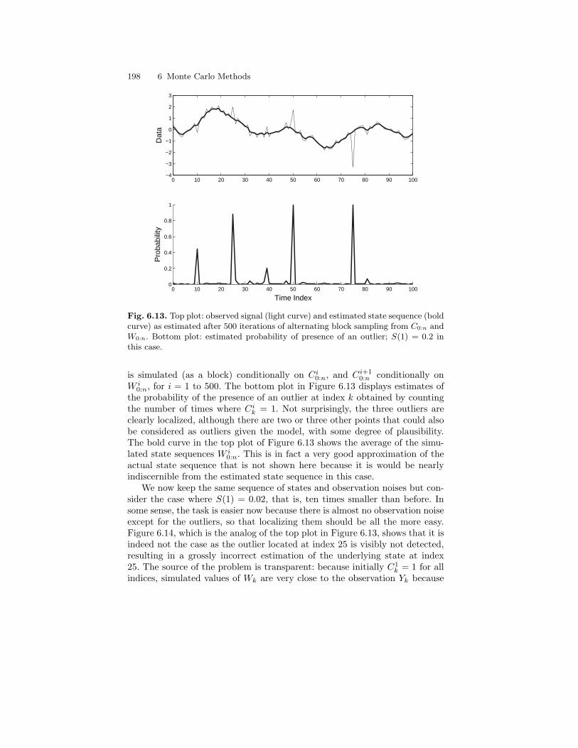
198 6 Monte Carlo Methods

0 10 20 30 40 50 60 70 80 90 1000

0.2

0.4

0.6

0.8

1

Time Index

Pro

babi

lity

0 10 20 30 40 50 60 70 80 90 100−4

−3

−2

−1

0

1

2

3

Dat

a

Fig. 6.13. Top plot: observed signal (light curve) and estimated state sequence (boldcurve) as estimated after 500 iterations of alternating block sampling from C0:n andW0:n. Bottom plot: estimated probability of presence of an outlier; S(1) = 0.2 inthis case.

is simulated (as a block) conditionally on Ci0:n, and Ci+10:n conditionally on

W i0:n, for i = 1 to 500. The bottom plot in Figure 6.13 displays estimates of

the probability of the presence of an outlier at index k obtained by countingthe number of times where Cik = 1. Not surprisingly, the three outliers areclearly localized, although there are two or three other points that could alsobe considered as outliers given the model, with some degree of plausibility.The bold curve in the top plot of Figure 6.13 shows the average of the simu-lated state sequences W i

0:n. This is in fact a very good approximation of theactual state sequence that is not shown here because it is would be nearlyindiscernible from the estimated state sequence in this case.

We now keep the same sequence of states and observation noises but con-sider the case where S(1) = 0.02, that is, ten times smaller than before. Insome sense, the task is easier now because there is almost no observation noiseexcept for the outliers, so that localizing them should be all the more easy.Figure 6.14, which is the analog of the top plot in Figure 6.13, shows that it isindeed not the case as the outlier located at index 25 is visibly not detected,resulting in a grossly incorrect estimation of the underlying state at index25. The source of the problem is transparent: because initially C1

k = 1 for allindices, simulated values of Wk are very close to the observation Yk because

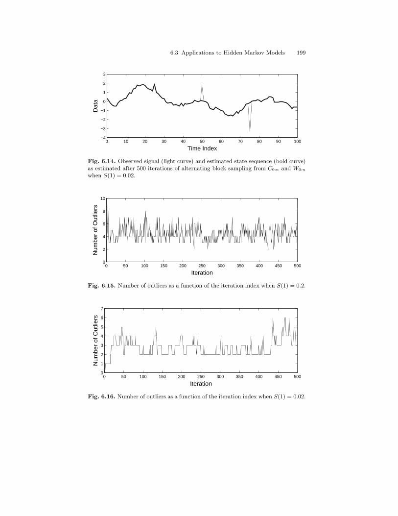
6.3 Applications to Hidden Markov Models 199

0 10 20 30 40 50 60 70 80 90 100−4

−3

−2

−1

0

1

2

3

Dat

a

Time Index

Fig. 6.14. Observed signal (light curve) and estimated state sequence (bold curve)as estimated after 500 iterations of alternating block sampling from C0:n and W0:n

when S(1) = 0.02.

0 50 100 150 200 250 300 350 400 450 5000

2

4

6

8

10

Iteration

Num

ber

of O

utlie

rs

Fig. 6.15. Number of outliers as a function of the iteration index when S(1) = 0.2.

0 50 100 150 200 250 300 350 400 450 5000

1

2

3

4

5

6

7

Iteration

Num

ber

of O

utlie

rs

Fig. 6.16. Number of outliers as a function of the iteration index when S(1) = 0.02.

200 6 Monte Carlo Methods

S(1) is very small, in turn making it very difficult to reach configurations withCk = 2.

This lack of convergence when S(1) = 0.02 is also patent when comparingFigures 6.15 and 6.16: both figures show the simulated number of outliers, thatis, the number of indices k for which Cik = 2, as a function of the iterationindex i. In Figure 6.15, this number directly jumps from 0 initially to reachthe most likely values (between 3 and 6) and move very quickly in subsequentiterations. In contrast, in Figure 6.16 the estimated number of outliers variesonly very slowly with very long steady period. A closer examination of theoutput reveals that in the second case, it is only after 444 iterations that C26

is finally simulated as 2, which explains why the estimated sequence of statesis still grossly wrong after 500 simulations.

The moral of Example 6.3.3 is by no means that the case where S(1) = 0.02is desperate. Running the simulation for much longer than 500 iterations—andonce again, 500 is not considered as a big number in the MCMC world—doesproduce the expected results. On the other hand, the observation that thesame sampling algorithm performs significantly worse in a task that is ar-guably easier is not something that can easily be swept under the carpet. Atthe risk of frightening newcomers to the field, it is important to underlinethat this is not an entirely lonely observation, as it is often difficult to sampleefficiently from very concentrated distributions. In Example 6.3.3, the subsetsof (C ×W)n+1 that have non-negligible probability under the posterior dis-tribution are very narrow (in some suitable sense) and thus hard to explorewith generic MCMC approaches.

To overcome the limits of the method used so far, we can however takeprofit of the remark that in CGLSSMs, the conditional distribution of thecontinuous component of the state, W0:n, given both the observations Y0:n

and the sequence of indicators C0:n, is multivariate Gaussian and can be fullycharacterized using the algorithms discussed in Section 5.2. Hence the ideato devise MCMC algorithms that target the conditional distribution of C0:n

given Y0:n, where the continuous part W0:n is marginalized out, rather thanthe joint distribution of C0:n and W0:n. This is the principle of the approachesproposed by Carter and Kohn (1996) and Doucet and Andrieu (2001). Thespecific contribution of Doucet and Andrieu (2001) was to remark that us-ing the information form of the backward smoothing recursion (discussed inSection 5.2.5) is preferable because it is more generally applicable.

The main tool here is Lemma 5.2.24, which makes it possible to evaluatethe likelihood of the observations, marginalizing with respect to the contin-uous part of the state sequence, where all indicators except one are fixed.Combined with the information provided by the prior distribution of the se-quence of indicators, this is all we need for sampling an indicator given allits neighbors, which is the Gibbs sampling strategy discussed in full gener-ality in Section 6.2.5. There is however one important detail concerning theapplication Lemma 5.2.24 that needs to be clarified. To apply Lemma 5.2.24

6.3 Applications to Hidden Markov Models 201

at index k, it is required that the results of both the filtering recursion forindex k − 1, Wk−1|k−1(C0:k−1), Σk−1|k−1(C0:k−1), as well as those of thebackward information recursion at index k, κk|n(Ck+1:n), Πk|n(Ck+1:n), beavailable. None of these two recursions is particularly simple as each step ofeach recursion involves in particular the inversion of a square matrix whosedimension is that of the continuous component of the state. The importantpoint noted by Carter and Kohn (1996) and Doucet and Andrieu (2001) isthat because the forward quantities at index k depend on indicators Cl forl ≤ k only and, conversely, the backward quantities depend on indicatorsCl such that l > k only, it is advantageous to use a systematic scan Gibbssampler that simulates Ck given its neighbors for k = 0, . . . , n (or in reverseorder) so as to avoid multiple evaluation of identical quantities. This how-ever makes the overall algorithm somewhat harder to describe because it isnecessary to carry out the Gibbs simulations and the forward (or backward)recursion simultaneously. The overall computational complexity of a completesweep of the Gibbs sampler is then only of the order of what it takes to im-plement Algorithm 5.2.13 or Proposition 5.2.21 for all indices k between 0and n, times the number r of possible values of the indicator, as these needto be enumerated exhaustively at each index. We now describe the version ofthe systematic scan Gibbs sampler that uses the result previously obtained inSection 5.2.6.

Algorithm 6.3.4 (Gibbs Sampler for Indicators in Conditional Gaus-sian Linear State-Space Model). Consider a conditionally Gaussian linearstate-space model (Definition 2.2.6) with indicator-dependent matrices A, R, B,and S for which the covariance of the initial state Σν may depend on C0 anddenote by νC and QC , respectively, the initial distribution and transition matrixof Ckk≥0.

Assuming that a current simulated sequence of indicators Ci0:n is available,draw Ci+1

0:n as follows.

Backward Recursion: Apply Proposition 5.2.21 for k = n down to 0 with Ak =A(Cik+1), Rk = R(Cik+1), Bk = B(Cik), and Sk = S(Cik). Store the com-puted quantities κk|n and Πk|n for k = n down to 0.

Initial State: For c = 1, . . . , r, compute

ε0 = Y0 ,

Γ0(c) = B(c)Σν(c)Bt(c) + S(c)St(c) ,

W0|0(c) = Σν(c)Bt(c)Γ−10 (c)ε0 ,

Σ0|0(c) = Σν(c)−Σν(c)Bt(c)Γ−10 (c)Bt(c)Σν(c) ,

`0(c) = −[log |Γ0(c)|+ εt0Γ

−10 (c)ε0

]/2

W0|n(c) = W0|0(c) +Σ0|0(c)[I +Π0|nΣ0|0(c)

]−1[κ0|n −Π0|nW0|0(c)

],

Σ0|n(c) = Σ0|0(c)−Σ0|0(c)[I +Π0|nΣ0|0(c)

]−1Π0|nΣ0|0(c) ,

202 6 Monte Carlo Methods

m0(c) = −[log |Σ0|0(c)|+ W t

0|0(c)Σ−10|0(c)W0|0(c)

]/2

+[log |Σ0|n(c)|+ W t

0|n(c)Σ−10|n(c)W0|n(c)

]/2 ,

p0(c) = exp [`0(c) +m0(c)] νC(c)QC(c, Ci1) .

Normalize the vector p0 by computing p0(c) = p0(c)/∑rc′=1 p0(c′) for

c = 1, . . . , r and sample Ci+10 from the probability distribution p0 on

1, . . . , r. Then store the Kalman filter variables corresponding to c = Ci+10

(W0|0(Ci+10 ) and Σ0|0(Ci+1

0 ), that is) for the next iteration.

For k = 1, . . . , n: for c = 1, . . . , r, compute

Wk|k−1(c) = A(c)Wk−1|k−1(Ci+1k−1) ,

Σk|k−1(c) = A(c)Σk−1|k−1(Ci+1k−1)At(c) +R(c)Rt(c) ,

εk(c) = Yk −B(c)Wk|k−1(c) ,

Γk(c) = B(c)Σk|k−1(c)Bt(c) + S(c)St(c) ,

Wk|k(c) = Wk|k−1(c) +Σk|k−1(c)Bt(c)Γ−1k (c)εk(c) ,

Σk|k(c) = Σk|k−1(c)−Σk|k−1(c)Bt(c)Γ−1k (c)Bt(c)Σk|k−1(c) ,

`k(c) = −[log |Γk(c)|+ εtkΓ

−1k (c)εk

]/2 ,

Wk|n(c) = Wk|k(c) +Σk|k(c)[I +Πk|nΣk|k(c)

]−1[κk|n −Πk|nWk|k(c)

],

Σk|n(c) = Σk|k(c)−Σk|k(c)[I +Πk|nΣk|k(c)

]−1Πk|nΣk|k(c) ,

mk(c) = −[log |Σk|k(c)|+ W t

k|k(c)Σ−1k|k(c)Wk|k(c)

]/2

+[log |Σk|n(c)|+ W t

k|n(c)Σ−1k|n(c)Wk|n(c)

]/2 ,

pk(c) =

exp [`k(c) +mk(c)]QC(Ci+1k−1, c)QC(c, Cik+1) for k < n

exp [`n(c) +mn(c)]QC(Ci+1n−1, c) for k = n

.

Set pk(c) = pk(c)/∑rc′=1 pk(c′) (for c = 1, . . . , r) and sample Ci+1

k from

pk. If k < n, the corresponding Kalman filter variables Wk|k(Ci+1k ) and

Σk|k(Ci+1k ) are stored for the next iteration.

Despite the fact that it is perhaps the most complex algorithm that isto be met in this book, Algorithm 6.3.4 deserves no special comment asit simply combines the results obtained in Chapter 5 (Algorithms 5.2.13and 5.2.22, Lemma 5.2.24) with the principle of the Gibbs sampler exposedin Section 6.2.5 and the clever remark that using a systematic scanning orderof the simulation sites (here in ascending order) greatly reduces the compu-tation load. Algorithm 6.3.4 is similar to the method described by Doucetand Andrieu (2001), but here the expression used for evaluating mk(c) hasbeen made more transparent by use of the smoothing moments Wk|n(c) andΣk|n(c).

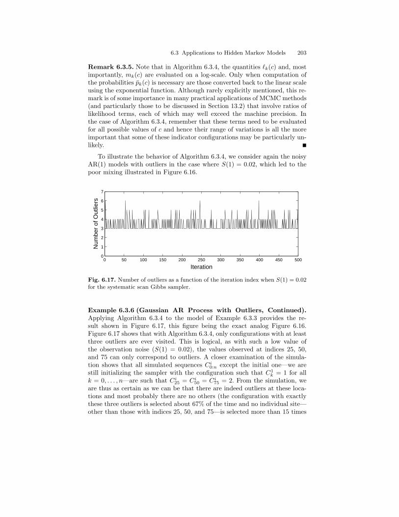
6.3 Applications to Hidden Markov Models 203

Remark 6.3.5. Note that in Algorithm 6.3.4, the quantities `k(c) and, mostimportantly, mk(c) are evaluated on a log-scale. Only when computation ofthe probabilities pk(c) is necessary are those converted back to the linear scaleusing the exponential function. Although rarely explicitly mentioned, this re-mark is of some importance in many practical applications of MCMC methods(and particularly those to be discussed in Section 13.2) that involve ratios oflikelihood terms, each of which may well exceed the machine precision. Inthe case of Algorithm 6.3.4, remember that these terms need to be evaluatedfor all possible values of c and hence their range of variations is all the moreimportant that some of these indicator configurations may be particularly un-likely.

To illustrate the behavior of Algorithm 6.3.4, we consider again the noisyAR(1) models with outliers in the case where S(1) = 0.02, which led to thepoor mixing illustrated in Figure 6.16.

0 50 100 150 200 250 300 350 400 450 5000

1

2

3

4

5

6

7

Iteration

Num

ber

of O

utlie

rs

Fig. 6.17. Number of outliers as a function of the iteration index when S(1) = 0.02for the systematic scan Gibbs sampler.

Example 6.3.6 (Gaussian AR Process with Outliers, Continued).Applying Algorithm 6.3.4 to the model of Example 6.3.3 provides the re-sult shown in Figure 6.17, this figure being the exact analog Figure 6.16.Figure 6.17 shows that with Algorithm 6.3.4, only configurations with at leastthree outliers are ever visited. This is logical, as with such a low value ofthe observation noise (S(1) = 0.02), the values observed at indices 25, 50,and 75 can only correspond to outliers. A closer examination of the simula-tion shows that all simulated sequences Ci0:n except the initial one—we arestill initializing the sampler with the configuration such that C1

k = 1 for allk = 0, . . . , n—are such that Ci25 = Ci50 = Ci75 = 2. From the simulation, weare thus as certain as we can be that there are indeed outliers at these loca-tions and most probably there are no others (the configuration with exactlythese three outliers is selected about 67% of the time and no individual site—other than those with indices 25, 50, and 75—is selected more than 15 times

204 6 Monte Carlo Methods

out of the 500 iterations). Figure 6.17 also shows that the other configurationsthat are explored are visited rather rapidly rather than with long idle periodsas in Figure 6.16, which also suggests good mixing properties of the Gibbssampling algorithm.

To conclude this section with a more realistic example of the use ofCGLSSMs and MCMC techniques, we consider the change point model andthe well-log data already discussed in Example 1.3.10.

Example 6.3.7 (Gibbs Sampler for the Well-Log Data). To analyzethe well-log data shown in Figure 1.7, we consider the conditionally Gaussianstate-space model

Wk+1 = A(Ck+1,1)Wk +R(Ck+1,1)Uk , Uk ∼ N(0, 1) ,Yk = µY (Ck,2) +B(Ck,2)Wk + S(Ck,2)Vk , Vk ∼ N(0, 1) ,

where Ck,1 ∈ 1, 2 and Ck,2 ∈ 1, 2 are indicator variables indicating, re-spectively, the presence of a jump in the level of the underlying signal and thatof an outlier in the measurement noise, as discussed in Examples 1.3.10 and1.3.11. For comparison purposes, we use exactly the same model specificationas the one advocated by Fearnhead and Clifford (2003).

• The data shown in Figure 1.7 is first centered (approximately) by sub-tracting µ = 115, 000 from each observation; in the following, Yk refers tothe data with this average level µ subtracted.

• When Ck,1 = 1 the underlying signal level is constant and we set A(1) = 1and R(1) = 0. When Ck,1 = 2, the occurrence of a jump is modeledby A(2) = 0, R(2) = 10,000, which is an informative prior on the sizeof the jump. Though as explained in the introduction this is presumablyan oversimplified assumption, we assume a constant probability for thepresence of a jump, or, equivalently, that Ck,1k≥0 is an i.i.d. sequenceof Bernoulli random variables with constant probability of success p. Thejump positions then form a discrete renewal sequence whose incrementdistribution is geometric with expectation 1/p. Because there are about16 jumps in a sequence of 4,000 samples, the average of the incrementdistribution is about 250, suggesting p = 1/250.

• When Ck,2 = 1, the observation is modeled as the true state corruptedby additive noise, so that B(1) = 1, where S(1) is set to 2,500 basedon the empirical standard deviation of the median filter residual shownin the right plot of Figure 1.7. When Ck,2 = 2, the occurrence of anoutlier is modeled by a Gaussian random variable whose parameters areindependent of the true state, so that B(2) = 0, and the outlier is assumedto have mean µY (2) = -30,000 and standard deviation S(2) = 12,500.The outliers appear to be clustered in time, with a typical cluster sizeof four samples. Visual inspection shows that there are about 16 clustersof noise, which suggests to model the sequence Ck,2k≥0 as a Markov

6.3 Applications to Hidden Markov Models 205

chain with transition probabilities P(Ck,2 = 2 |Ck,2 = 1) = 1/250 andP(Ck,2 = 1 |Ck,2 = 2) = 1/4. The initial C0,2 is assumed to be distributedaccording to the stationary distribution of this chain, which is P(C0,2 =1) = 125/127.

• The initial distribution of W0 is assumed to have zero mean with a verylarge variance, which corresponds to an approximation of the so-calleddiffuse (or improper flat, following the terminology of Section 5.2.5) prior.Note that because B(C0) may be null (when C0 = 2), using a truly diffuseprior (with “infinite” covariance matrix) cannot be done in this case bysimply computing W0|0 as in (5.109), which is customary. In the case underconsideration, however, the prior on W0 is non-essential because the initialstate is very clearly identified from the data anyway.

Note that in the model above, the presence of outliers induces non-zero meansin the observation equation. As discussed in Remark 5.2.14, however, thisdoes not necessitate significant modifications, and we just need to applyAlgorithm 6.3.4 using as “observation” Yk − µY (ck) rather than Yk, whereµY (1) = 0 and µY (2) = -30,000.

Because R(1) = 0 implies that the continuous component of the state Wk

stays exactly constant between two jump points, this model belongs to thecategory discussed earlier for which the alternating block sampling algorithmcannot be applied at all. We thus consider the result of the Gibbs samplerthat operates on the indicator variables only. Figure 6.18 displays the resultsobtained by application of Algorithm 6.3.4 after 5,000 iterations, one itera-tion referring to a complete cycle of the Gibbs sampler through all the n+ 1sites. Initially, C1

k,1 and C1k,2 are both set to 1 for all sites k = 0, . . . , n, which

corresponds to the (very improbable) configuration in which there are neitherjumps nor outliers. Clearly, after 5,000 iterations both the jump and outlierpositions are located very clearly. There is however a marked difference, whichis that whereas the outliers (middle plot) are located with posterior probabil-ities very close to 1, the jumps are only located with probabilities between 0.3and 0.6. There are two reasons for this behavior, the second being more fun-damental. First, the model for the distribution of outliers is more precise andincorporate in particular the fact that outliers systematically induce a down-ward bias. The second reason is a slightly deficient modeling of the occurrenceof jumps. For the outliers, the selected Markov transition kernel implies thatoutlier periods are infrequent (occurring 2/127 of the time on average) buthave durations that are exponential with average duration 4. This is a crucialfeature, as a closer examination of the data reveals that some of these periodsof outliers last for 10 or even 20 consecutive samples. In contrast, our model forjumps implies that jumps are infrequent (occurring in one sample out of 250on average) and isolated. For instance, a sequence of four consecutive jumpsis, a priori, judged as being 6.2× 107 times less probable than the occurrenceof just one jump in one of these four positions. The real data however, cf.Figure 6.19, shows that the actual jumps are not abrupt and involve at least

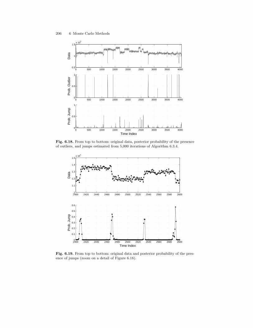
206 6 Monte Carlo Methods

0 500 1000 1500 2000 2500 3000 3500 40000

0.5

1

Pro

b. J

ump

Time Index

0 500 1000 1500 2000 2500 3000 3500 40000

0.5

1

Pro

b. O

utlie

r0 500 1000 1500 2000 2500 3000 3500 4000

0.5

1

1.5x 10

5

Dat

a

Fig. 6.18. From top to bottom: original data, posterior probability of the presenceof outliers, and jumps estimated from 5,000 iterations of Algorithm 6.3.4.

2400 2420 2440 2460 2480 2500 2520 2540 2560 2580 26000

0.1

0.2

0.3

0.4

0.5

0.6

Pro

b. J

ump

Time Index

2400 2420 2440 2460 2480 2500 2520 2540 2560 2580 26001

1.1

1.2

1.3

1.4

1.5x 10

5

Dat

a

Fig. 6.19. From top to bottom: original data and posterior probability of the pres-ence of jumps (zoom on a detail of Figure 6.18).

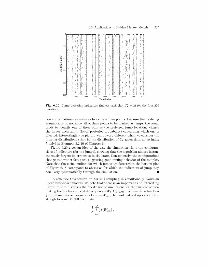
6.3 Applications to Hidden Markov Models 207

0 500 1000 1500 2000 2500 3000 3500 4000

0

50

100

150

200

250

Time Index

Sim

ulat

ion

Inde

x

Fig. 6.20. Jump detection indicators (indices such that Cik = 2) for the first 250

iterations.

two and sometimes as many as five consecutive points. Because the modelingassumptions do not allow all of these points to be marked as jumps, the resulttends to identify one of these only as the preferred jump location, whencethe larger uncertainty (lower posterior probability) concerning which one isselected. Interestingly, the picture will be very different when we consider thefiltering distributions (that is, the distribution of Ck given data up to indexk only) in Example 8.2.10 of Chapter 8.

Figure 6.20 gives an idea of the way the simulation visits the configura-tions of indicators (for the jumps), showing that the algorithm almost instan-taneously forgets its erroneous initial state. Consequently, the configurationschange at a rather fast pace, suggesting good mixing behavior of the sampler.Note that those time indices for which jumps are detected in the bottom plotof Figure 6.18 correspond to abscissas for which the indicators of jump stay“on” very systematically through the simulation.

To conclude this section on MCMC sampling in conditionally Gaussianlinear state-space models, we note that there is an important and interestingliterature that discusses the “best” use of simulations for the purpose of esti-mating the unobservable state sequence Wk, Ckk≥0. To estimate a functionf of the unobserved sequence of states W0:n, the most natural options are thestraightforward MCMC estimate

1N

N∑i=1

f(W i0:n) ,

208 6 Monte Carlo Methods

directly available with alternating block sampling (as in Example 6.3.3), orits Rao-Blackwellized version

1N

N∑i=1

E[f(W0:n) |Ci0:n] ,

which can easily be computed when using Algorithm 6.3.4, at least for linearand quadratic functions f , as the smoothing moments Wk|n(Ci+1

0:k , Cik+1:n) and

Σk|n(Ci+10:k , C

ik+1:n) are evaluated at each iteration i and for all sites k. But

both of these alternatives are estimates of E[f(W0:n) |Y0:n], which, in someapplications, is perhaps not what is regarded as the “best” estimate of thestates. In the change point application discussed in Example 6.3.7 in particu-lar, E [f(W0:n) |Y0:n] does not correspond to a piecewise constant trajectory,especially if some jump locations are only detected with some ambiguity. Ifone really believes that the model is correct, it may thus make more senseto estimate first the best sequence of indicators c0:n, that is, the one thatmaximizes P(C0:n = c0:n |Y0:n), and then use E[f(W0:n) |Y0:n, C0:n = c0:n]as the estimate of the continuous part of the state sequence. In the changepoint model, this third way of proceeding is guaranteed to return a piecewiseconstant sequence. This is not an easy task, however, because finding the in-dicator sequence c0:n that maximizes the posterior probability is a difficultcombinatorial optimization problem, especially given the fact that we can-not evaluate P(C0:n = c0:n |Y0:n) directly. We refer to Lavielle and Lebarbier(2001), Doucet and Andrieu (2001), and references therein for further readingon this issue.

7

Sequential Monte Carlo Methods

The use of Monte Carlo methods for non-linear filtering can be traced back tothe pioneering contributions of Handschin and Mayne (1969) and Handschin(1970). These early attempts were based on sequential versions of the impor-tance sampling paradigm, a technique that amounts to simulating samplesunder an instrumental distribution and then approximating the target distri-butions by weighting these samples using appropriately defined importanceweights. In the non-linear filtering context, importance sampling algorithmscan be implemented sequentially in the sense that, by defining carefully asequence of instrumental distributions, it is not needed to regenerate the pop-ulation of samples from scratch upon the arrival of each new observation. Thisalgorithm is called sequential importance sampling, often abbreviated SIS. Al-though the SIS algorithm has been known since the early 1970s, its use innon-linear filtering problems was rather limited at that time. Most likely, theavailable computational power was then too limited to allow convincing appli-cations of these methods. Another less obvious reason is that the SIS algorithmsuffers from a major drawback that was not clearly identified and properlycured until the seminal paper by Gordon et al. (1993). As the number of it-erations increases, the importance weights tend to degenerate, a phenomenonknown as sample impoverishment or weight degeneracy. Basically, in the longrun most of the samples have very small normalized importance weights andthus do not significantly contribute to the approximation of the target distri-bution. The solution proposed by Gordon et al. (1993) is to allow rejuvenationof the set of samples by duplicating the samples with high importance weightsand, on the contrary, removing samples with low weights.

The particle filter of Gordon et al. (1993) was the first successful applica-tion of sequential Monte Carlo techniques to the field of non-linear filtering.Since then, sequential Monte Carlo (or SMC) methods have been applied inmany different fields including computer vision, signal processing, control,econometrics, finance, robotics, and statistics (Doucet et al., 2001a; Risticet al., 2004). This chapter reviews the basic building blocks that are neededto implement a sequential Monte Carlo algorithm, starting with concepts re-

210 7 Sequential Monte Carlo Methods

lated to the importance sampling approach. More specific aspects of sequentialMonte Carlo techniques will be further discussed in Chapter 8, while conver-gence issues will be dealt with in Chapter 9.

7.1 Importance Sampling and Resampling

7.1.1 Importance Sampling

Importance sampling is a method that dates back to, at least, Hammersley andHandscomb (1965) and that is commonly used in several fields (for generalreferences on importance sampling, see Glynn and Iglehart, 1989, Geweke,1989, Evans and Swartz, 1995, or Robert and Casella, 2004.)

Throughout this section, µ will denote a probability measure of intereston a measurable space (X,X ), which we shall refer to as the target distri-bution. As in Chapter 6, the aim is to approximate integrals of the formµ(f) =

∫Xf(x)µ(dx) for real-valued measurable functions f . The Monte Carlo

approach exposed in Section 6.1 consists in drawing an i.i.d. sample ξ1, . . . ,ξN from the probability measure µ and then evaluating the sample meanN−1

∑Ni=1 f(ξi). Of course, this technique is applicable only when it is possi-

ble (and reasonably simple) to sample from the target distribution µ.Importance sampling is based on the idea that in certain situations it is

more appropriate to sample from an instrumental distribution ν, and then toapply a change-of-measure formula to account for the fact that the instru-mental distribution is different from the target distribution. More formally,assume that the target probability measure µ is absolutely continuous withrespect to an instrumental probability measure ν from which sampling is easilyfeasible. Denote by dµ/dν the Radon-Nikodym derivative of µ with respectto ν. Then for any µ-integrable function f ,

µ(f) =∫f(x)µ(dx) =

∫f(x)

dµ

dν(x) ν(dx) . (7.1)

In particular, if ξ1, ξ2, . . . is an i.i.d. sample from ν, (7.1) suggests the followingestimator of µ(f):

µISν,N (f) = N−1

N∑i=1

f(ξi)dµ

dν(ξi) . (7.2)

Because this estimator is the sample mean of independent random variables,there is a range of results to assess the quality of µIS

ν,N (f) as an estimatorof µ(f). First of all, the strong law of large number implies that µIS

ν,N (f)converges to µ(f) almost surely as N tends to infinity. In addition, the cen-tral limit theorem for i.i.d. variables (or deviation inequalities) may serve asa guidance for selecting the proposal distribution ν, beyond the obvious re-quirement that it should dominate the target distribution µ. We postpone this

7.1 Importance Sampling and Resampling 211

issue and, more generally, considerations that pertain to the behavior of theapproximation for large values of N to Chapter 9.

In many situations, the target probability measure µ or the instrumentalprobability measure ν is known only up to a normalizing factor. As alreadydiscussed in Remark 6.2.7, this is particularly true when applying impor-tance sampling ideas to HMMs and, more generally, in Bayesian statistics.The Radon-Nikodym derivative dµ/dν is then known up to a (constant) scal-ing factor only. It is however still possible to use the importance samplingparadigm in that case, by adopting the self-normalized form of the impor-tance sampling estimator,

µISν,N (f) =

∑Ni=1 f(ξi)dµdν (ξi)∑N

i=1dµdν (ξi)

. (7.3)

This quantity is obviously free from any scale factor in dµ/dν. The self-normalized importance sampling estimator µIS

ν,N (f) is defined as a ratio of thesample means of the functions f1 = f × (dµ/dν) and f2 = dµ/dν. The stronglaw of large numbers thus implies that N−1

∑Ni=1 f1(ξi) and N−1

∑Ni=1 f2(ξi)

converge almost surely, to µ(f1) and ν(dµ/dν) = 1, respectively, showing thatµISν,N (f) is a consistent estimator of µ(f). Again, more precise results on the

behavior of this estimator will be given in Chapter 9. In the following, theterm importance sampling usually refers to the self-normalized form (7.3) ofthe importance sampling estimate.

7.1.2 Sampling Importance Resampling

Although importance sampling is primarily intended to overcome difficul-ties with direct sampling from µ when approximating integrals of the formµ(f), it can also be used for (approximate) sampling from the distribution µ.The latter can be achieved by the sampling importance resampling (or SIR)method due to Rubin (1987, 1988). Sampling importance resampling is a two-stage procedure in which importance sampling as discussed below is followedby an additional random sampling step. In the first stage, an i.i.d. sample(ξ1, . . . , ξM ) is drawn from the instrumental distribution ν, and one computesthe normalized version of the importance weights,

ωi =dµdν (ξi)∑Mi=1

dµdν (ξi)

, i = 1, . . . ,M . (7.4)

In the second stage, the resampling stage, a sample of size N denoted byξ1, . . . , ξN is drawn from the intermediate set of points ξ1, . . . , ξM , takinginto account the weights computed in (7.4). The rationale is that points ξi forwhich ωi in (7.4) is large are most likely under the target distribution µ andshould thus be selected with higher probability during the resampling than

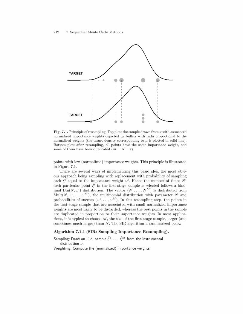
212 7 Sequential Monte Carlo Methods

TARGET

TARGET

Fig. 7.1. Principle of resampling. Top plot: the sample drawn from ν with associatednormalized importance weights depicted by bullets with radii proportional to thenormalized weights (the target density corresponding to µ is plotted in solid line).Bottom plot: after resampling, all points have the same importance weight, andsome of them have been duplicated (M = N = 7).

points with low (normalized) importance weights. This principle is illustratedin Figure 7.1.

There are several ways of implementing this basic idea, the most obvi-ous approach being sampling with replacement with probability of samplingeach ξi equal to the importance weight ωi. Hence the number of times N i

each particular point ξi in the first-stage sample is selected follows a bino-mial Bin(N,ωi) distribution. The vector (N1, . . . , NM ) is distributed fromMult(N,ω1, . . . , ωM ), the multinomial distribution with parameter N andprobabilities of success (ω1, . . . , ωM ). In this resampling step, the points inthe first-stage sample that are associated with small normalized importanceweights are most likely to be discarded, whereas the best points in the sampleare duplicated in proportion to their importance weights. In most applica-tions, it is typical to choose M , the size of the first-stage sample, larger (andsometimes much larger) than N . The SIR algorithm is summarized below.

Algorithm 7.1.1 (SIR: Sampling Importance Resampling).

Sampling: Draw an i.i.d. sample ξ1, . . . , ξM from the instrumentaldistribution ν.

Weighting: Compute the (normalized) importance weights

7.1 Importance Sampling and Resampling 213

ωi =dµdν (ξi)∑Mj=1

dµdν (ξj)

for i = 1, . . . ,M .

Resampling:• Draw, conditionally independently given (ξ1, . . . , ξM ), N discrete random

variables (I1, . . . , IN ) taking values in the set 1, . . . ,M with probabil-ities (ω1, . . . , ωM ), i.e.,

P(I1 = j) = ωj , j = 1, . . . ,M . (7.5)

• Set, for i = 1, . . . , N , ξi = ξIi

.

The set (I1, . . . , IN ) is thus a multinomial trial process. Hence, this methodof selection is known as the multinomial resampling scheme.

At this point, it may not be obvious that the sample ξ1, . . . , ξN obtainedfrom Algorithm 7.1.1 is indeed (approximately) i.i.d. from µ in any suitablesense. In Chapter 9, it will be shown that the sample mean of the drawsobtained using the SIR algorithm,

µSIRν,M,N (f) =

1N

N∑i=1

f(ξi) , (7.6)

is a consistent estimator of µ(f) for all functions f satisfying µ(|f |) <∞. Theresampling step might thus be seen as a means to transform the weightedimportance sampling estimate µIS

ν,M (f) defined by (7.3) into an unweightedsample average. Recall that N i is the number of times that the element ξi isresampled. Rewriting

µSIRν,M,N (f) =

1N

N∑i=1

f(ξi) =M∑i=1

N i

Nf(ξi) ,

it is easily seen that the sample mean µSIRν,M,N (f) of the SIR sample is, condi-

tionally on the first-stage sample (ξ1, . . . , ξM ), equal to the importance sam-pling estimator µIS

ν,M (f) defined in (7.3),

E[µSIRν,M,N (f)

∣∣ ξ1, . . . , ξM]

= µISν,M (f) .

As a consequence, the SIR estimator µSIRν,M,N (f) is an unbiased estimate of

µ(f), but its mean squared error is always larger than that of the importancesampling estimator (7.3) due to the well-known variance decomposition

E[(µSIRν,M,N (f)− µ(f)

)2]= E

[(µSIRν,M,N (f)− µIS

ν,M (f))2]

+ E[(µISν,M (f)− µ(f)

)2].

214 7 Sequential Monte Carlo Methods

The variance E[(µSIRν,M,N (f) − µIS

ν,M (f))2] may be interpreted as the priceto pay for converting the weighted importance sampling estimate into anunweighted approximation.

Showing that the SIR estimate (7.6) is a consistent and asymptoticallynormal estimator of µ(f) is not a trivial task, as ξ1, . . . , ξN are no moreindependent due to the normalization of the weights followed by resampling.As such, the elementary i.i.d. convergence results that underlie the theory ofthe importance sampling estimator are of no use, and we refer to Section 9.2for the corresponding proofs.

Remark 7.1.2. A closer examination of the numerical complexity of Algo-rithm 7.1.1 reveals that whereas all steps of the algorithm have a complexitythat grows in proportion to M and N , this is not quite true for the multi-nomial sampling step whose numerical complexity is, a priori, growing fasterthan N (about N log2M—see Section 7.4.1 below for details). This is veryunfortunate, as we know from elementary arguments discussed in Section 6.1that Monte Carlo methods are most useful when N is large (or more appro-priately that the quality of the approximation improves rather slowly as Ngrows).

A clever use of elementary probabilistic results however makes it possibleto devise methods for sampling N times from a multinomial distribution withM possible outcomes using a number of operations that grows only linearlywith the maximum of N and M . In order not to interrupt our exposition ofsequential Monte Carlo, the corresponding algorithms are discussed in Sec-tion 7.4.1 at the end of this chapter. Note that we are here only discussing im-plementations issues. There are however different motivations, also discussedin Section 7.4.2, for adopting sampling schemes other than multinomial sam-pling.

7.2 Sequential Importance Sampling

7.2.1 Sequential Implementation for HMMs

We now specialize the sampling techniques considered above to hidden Markovmodels. As in previous chapters, we adopt the hidden Markov model as spec-ified by Definition 2.2.2 where Q denotes the Markov transition kernel of thehidden chain, ν is the distribution of the initial state X0, and g(x, y) (forx ∈ X, y ∈ Y) denotes the transition density function of the observation giventhe state, with respect to the measure µ on (Y,Y). To simplify the mathe-matical expressions, we will also use the shorthand notation gk(·) = g(·, Yk)introduced in Section 3.1.4. We denote the joint smoothing distribution byφ0:k|k, omitting the dependence with respect to the initial distribution ν,which does not play an important role here. According to (4.1), the joint

7.2 Sequential Importance Sampling 215

smoothing distribution may be updated recursively in time according to therelations

φ0(f) =∫f(x0) g0(x0) ν(dx0)∫

g0(x0) ν(dx0)for all f ∈ Fb (X) ,

φ0:k+1|k+1(fk+1) =∫· · ·∫fk+1(x0:k+1) φ0:k|k(dx0:k)T u

k (xk, dxk+1)

for all fk+1 ∈ Fb

(Xk+2

), (7.7)

where T uk is the transition kernel on (X,X ) defined by

T uk (x, f) =

(Lk+1

Lk

)−1 ∫f(x′)Q(x, dx′)gk+1(x′)

for all x ∈ X, f ∈ Fb (X) . (7.8)

The superscript “u” (for “unnormalized”) in the notation T uk is meant to high-

light the fact that T uk is not a probability transition kernel. This distinction is

important here because the normalized version Tk = T uk /T

uk (1) of the kernel

will play an important role in the following. Note that except in some spe-cial cases discussed in Chapter 5, the likelihood ratio Lk+1/Lk can generallynot be computed in closed form, rendering analytic evaluation of T u

k or φ0:k|khopeless. The rest of this section reviews importance sampling methods thatmake it possible to approximate φ0:k|k recursively in k.

First, because importance sampling can be used when the target distri-bution is known only up to a scaling factor, the presence of non-computableconstants such as Lk+1/Lk does not preclude the use of the algorithm. Next, itis convenient to choose the instrumental distribution as the probability mea-sure associated with a possibly non-homogeneous Markov chain on X. As seenbelow, this will make it possible to derive a sequential version of the impor-tance sampling technique. Let Rkk≥0 denote a family of Markov transitionkernels on (X,X ) and let ρ0 denote a probability measure on (X,X ). Furtherdenote by ρ0:kk≥0 the family of probability measures associated with the in-homogeneous Markov chain with initial distribution ρ0 and transition kernelsRkk≥0,

ρ0:k(fk) def=∫· · ·∫fk(x0:k) ρ0(dx0)

k−1∏l=0

Rl(xl, dxl+1) .

In this context, the kernels Rk will be referred to as the instrumental kernels.The term importance kernel is also used. The following assumptions will beadopted in the sequel.

216 7 Sequential Monte Carlo Methods

Assumption 7.2.1 (Sequential Importance Sampling).

1. The target distribution φ0 is absolutely continuous with respect to the in-strumental distribution ρ0.

2. For all k ≥ 0 and all x ∈ X, the measure T uk (x, ·) is absolutely continuous

with respect to Rk(x, ·).

Then for any k ≥ 0 and any function fk ∈ Fb

(Xk+1

),

φ0:k|k(fk) =∫· · ·∫fk(x0:k)

dφ0

dρ0(x0)

k−1∏l=0

dT ul (xl, ·)

dRl(xl, ·)(xl+1)

ρ0:k(dx0:k) ,

(7.9)which implies that the target distribution φ0:k|k is absolutely continuous withrespect to the instrumental distribution ρ0:k with Radon-Nikodym derivativegiven by

dφ0:k|k

dρ0:k(x0:k) =

dφ0

dρ0(x0)

k−1∏l=0

dT ul (xl, ·)

dRi(xl, ·)(xl+1) . (7.10)

It is thus legitimate to use ρ0:k as an instrumental distribution to computeimportance sampling estimates for integrals with respect to φ0:k|k. Denotingby ξ1

0:k, . . . , ξN0:k N i.i.d. random sequences with common distribution ρ0:k, the

importance sampling estimate of φ0:k|k(fk) for fk ∈ Fb

(Xk+1

)is defined as

φIS0:k|k(fk) =

∑Ni=1 ω

ikfk(ξi0:k)∑Ni=1 ω

ik

, (7.11)

where ωik are the unnormalized importance weights defined recursively by

ωi0 =dφ0

dρ0(ξi0) for i = 1, . . . , N , (7.12)

and, for k ≥ 0,

ωik+1 = ωikdT u

k (ξik, ·)dRk(ξik, ·)

(ξik+1) for i = 1, . . . , N . (7.13)

The multiplicative decomposition of the (unnormalized) importance weightsin (7.13) implies that these weights may be computed recursively in time assuccessive observations become available. In the sequential Monte Carlo lit-erature, the update factor dT u

k /dRk is often called the incremental weight.As discussed previously in Section 7.1.1, the estimator in (7.11) is left un-modified if the weights, or equivalently the incremental weights, are evaluatedup to a constant only. In particular, one may omit the problematic scalingfactor Lk+1/Lk that we met in the definition of T u

k in (7.8). The practicalimplementation of sequential importance sampling thus goes as follows.

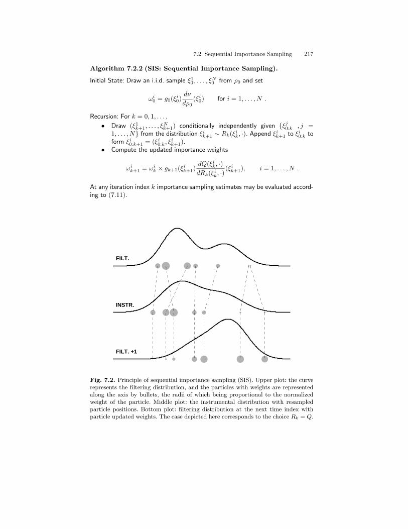
7.2 Sequential Importance Sampling 217

Algorithm 7.2.2 (SIS: Sequential Importance Sampling).

Initial State: Draw an i.i.d. sample ξ10 , . . . , ξ

N0 from ρ0 and set

ωi0 = g0(ξi0)dν

dρ0(ξi0) for i = 1, . . . , N .

Recursion: For k = 0, 1, . . . ,• Draw (ξ1

k+1, . . . , ξNk+1) conditionally independently given ξj0:k , j =

1, . . . , N from the distribution ξik+1 ∼ Rk(ξik, ·). Append ξik+1 to ξi0:k toform ξi0:k+1 = (ξi0:k, ξ

ik+1).

• Compute the updated importance weights

ωik+1 = ωik × gk+1(ξik+1)dQ(ξik, ·)dRk(ξik, ·)

(ξik+1), i = 1, . . . , N .

At any iteration index k importance sampling estimates may be evaluated accord-ing to (7.11).

FILT.

INSTR.

FILT. +1

Fig. 7.2. Principle of sequential importance sampling (SIS). Upper plot: the curverepresents the filtering distribution, and the particles with weights are representedalong the axis by bullets, the radii of which being proportional to the normalizedweight of the particle. Middle plot: the instrumental distribution with resampledparticle positions. Bottom plot: filtering distribution at the next time index withparticle updated weights. The case depicted here corresponds to the choice Rk = Q.

218 7 Sequential Monte Carlo Methods

An important feature of Algorithm 7.2.2, which corresponds to the methodoriginally proposed in Handschin and Mayne (1969) and Handschin (1970),is that the N trajectories ξ1

0:k, . . . , ξN0:k are independent and identically dis-

tributed for all time indices k. Following the terminology in use in the non-linear filtering community, we shall refer to the sample at time index k,ξ1k, . . . , ξ

Nk , as the population (or system) of particles and to ξi0:k for a specific

value of the particle index i as the history (or trajectory) of the ith particle.The principle of the method is illustrated in Figure 7.2.

7.2.2 Choice of the Instrumental Kernel

Before discussing in Section 7.3 a serious drawback of Algorithm 7.2.2 thatneeds to be fixed in order for the method to be applied to any problem of prac-tical interest, we examine strategies that may be helpful in selecting properinstrumental kernels Rk in several models (or families of models) of interest.

7.2.2.1 Prior Kernel

The first obvious and often very simple choice of instrumental kernel Rk is thatof setting Rk = Q (irrespectively of k). In that case, the instrumental kernelsimply corresponds to the prior distribution of the new state in the absenceof the corresponding observation. The incremental weight then simplifies to

dT uk (x, ·)

dQ(x, ·)(x′) =

LkLk+1

gk+1(x′) ∝ gk+1(x′) for all (x, x′) ∈ X2 . (7.14)

A distinctive feature of the prior kernel is that the incremental weight in (7.14)does not depend on x, that is, on the previous position. The use of the priorkernel Rk = Q is popular because sampling from the prior kernel Q is oftenstraightforward, and computing the incremental weight simply amounts toevaluating the conditional likelihood of the new observation given the currentparticle position. The prior kernel also satisfies the minimal requirement ofimportance sampling as stated in Assumption 7.2.1. In addition, because theimportance function reduces to gk+1, it is upper-bounded as soon as one canassume that supx∈X,y∈Y g(x, y) is finite, which (often) is a very mild condi-tion (see also Section 9.1). Despite these appealing properties, the use of theprior kernel can sometimes lead to poor performance, often manifesting it-self as a lack of robustness with respect to the values taken by the observedsequence Ykk≥0. The following example illustrates this problem in a verysimple situation.

Example 7.2.3 (Noisy AR(1) Model). To illustrate the potential prob-lems associated with the use of the prior kernel, Pitt and Shephard (1999)consider the simple model where the observations arise from a first-order lin-ear autoregression observed in noise,

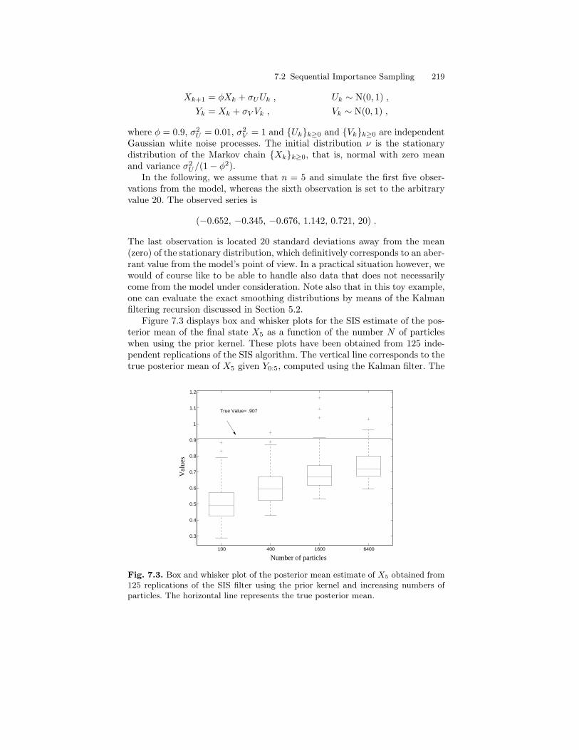
7.2 Sequential Importance Sampling 219

Xk+1 = φXk + σUUk , Uk ∼ N(0, 1) ,Yk = Xk + σV Vk , Vk ∼ N(0, 1) ,

where φ = 0.9, σ2U = 0.01, σ2

V = 1 and Ukk≥0 and Vkk≥0 are independentGaussian white noise processes. The initial distribution ν is the stationarydistribution of the Markov chain Xkk≥0, that is, normal with zero meanand variance σ2

U/(1− φ2).In the following, we assume that n = 5 and simulate the first five obser-

vations from the model, whereas the sixth observation is set to the arbitraryvalue 20. The observed series is

(−0.652, −0.345, −0.676, 1.142, 0.721, 20) .

The last observation is located 20 standard deviations away from the mean(zero) of the stationary distribution, which definitively corresponds to an aber-rant value from the model’s point of view. In a practical situation however, wewould of course like to be able to handle also data that does not necessarilycome from the model under consideration. Note also that in this toy example,one can evaluate the exact smoothing distributions by means of the Kalmanfiltering recursion discussed in Section 5.2.

Figure 7.3 displays box and whisker plots for the SIS estimate of the pos-terior mean of the final state X5 as a function of the number N of particleswhen using the prior kernel. These plots have been obtained from 125 inde-pendent replications of the SIS algorithm. The vertical line corresponds to thetrue posterior mean of X5 given Y0:5, computed using the Kalman filter. The

100 400 1600 6400

0.3

0.4

0.5

0.6

0.7

0.8

0.9

1

1.1

1.2

Val

ues

Number of particles

True Value= .907

Fig. 7.3. Box and whisker plot of the posterior mean estimate of X5 obtained from125 replications of the SIS filter using the prior kernel and increasing numbers ofparticles. The horizontal line represents the true posterior mean.

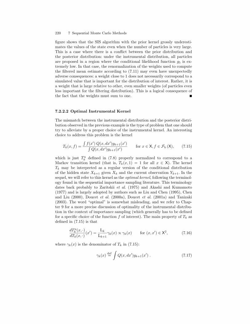
220 7 Sequential Monte Carlo Methods

figure shows that the SIS algorithm with the prior kernel grossly underesti-mates the values of the state even when the number of particles is very large.This is a case where there is a conflict between the prior distribution andthe posterior distribution: under the instrumental distribution, all particlesare proposed in a region where the conditional likelihood function g5 is ex-tremely low. In that case, the renormalization of the weights used to computethe filtered mean estimate according to (7.11) may even have unexpectedlyadverse consequences: a weight close to 1 does not necessarily correspond to asimulated value that is important for the distribution of interest. Rather, it isa weight that is large relative to other, even smaller weights (of particles evenless important for the filtering distribution). This is a logical consequence ofthe fact that the weights must sum to one.

7.2.2.2 Optimal Instrumental Kernel

The mismatch between the instrumental distribution and the posterior distri-bution observed in the previous example is the type of problem that one shouldtry to alleviate by a proper choice of the instrumental kernel. An interestingchoice to address this problem is the kernel

Tk(x, f) =∫f(x′)Q(x, dx′)gk+1(x′)∫Q(x, dx′)gk+1(x′)

for x ∈ X, f ∈ Fb (X), (7.15)

which is just T uk defined in (7.8) properly normalized to correspond to a

Markov transition kernel (that is, Tk(x, 1) = 1 for all x ∈ X). The kernelTk may be interpreted as a regular version of the conditional distributionof the hidden state Xk+1 given Xk and the current observation Yk+1. In thesequel, we will refer to this kernel as the optimal kernel, following the terminol-ogy found in the sequential importance sampling literature. This terminologydates back probably to Zaritskii et al. (1975) and Akashi and Kumamoto(1977) and is largely adopted by authors such as Liu and Chen (1995), Chenand Liu (2000), Doucet et al. (2000a), Doucet et al. (2001a) and Tanizaki(2003). The word “optimal” is somewhat misleading, and we refer to Chap-ter 9 for a more precise discussion of optimality of the instrumental distribu-tion in the context of importance sampling (which generally has to be definedfor a specific choice of the function f of interest). The main property of Tk asdefined in (7.15) is that

dT uk (x, ·)

dTk(x, ·)(x′) =

LkLk+1

γk(x) ∝ γk(x) for (x, x′) ∈ X2, (7.16)

where γk(x) is the denominator of Tk in (7.15):

γk(x) def=∫Q(x, dx′)gk+1(x′) . (7.17)

7.2 Sequential Importance Sampling 221

Equation (7.16) means that the incremental weight in (7.13) now dependson the previous position of the particle only (and not on the new positionproposed at index k+ 1). This is the exact opposite of the situation observedpreviously for the prior kernel. The optimal kernel (7.15) is attractive becauseit incorporates information both on the state dynamics and on the currentobservation: the particles move “blindly” with the prior kernel, whereas theytend to cluster into regions where the current local likelihood gk+1 is largewhen using the optimal kernel. There are however two problems with usingTk in practice. First, drawing from this kernel is usually not directly feasible.Second, calculation of the incremental importance weight γk in (7.17) maybe analytically intractable. Of course, the optimal kernel takes a simple formwith easy simulation and explicit evaluation of (7.17) in the particular casesdiscussed in Chapter 5. It turns out that it can also be evaluated for a slightlylarger class of non-linear Gaussian state-space models, as soon as the observa-tion equation is linear (Zaritskii et al., 1975). Indeed, consider the state-spacemodel with non-linear state evolution equation

Xk+1 = A(Xk) +R(Xk)Uk , Uk ∼ N(0, I) , (7.18)Yk = BXk + SVk , Vk ∼ N(0, I) , (7.19)

where A and R are matrix-valued functions of appropriate dimensions. Byapplication of Proposition 5.2.2, the conditional distribution of the state vectorXk+1 given Xk = x and Yk+1 is multivariate Gaussian with mean mk+1(x)and covariance matrix Σk+1(x), given by

Kk+1(x) = R(x)Rt(x)Bt[BR(x)Rt(x)Bt + SSt

]−1,

mk+1(x) = A(x) +Kk+1(x) [Yk+1 −BA(x)] ,

Σk+1(x) = [I −Kk+1(x)B]R(x)Rt(x) .

Hence new particles ξik+1 need to be simulated from the distribution

N(mk+1(ξik), Σk+1(ξik)

), (7.20)

and the incremental weight for the optimal kernel is proportional to

γk(x) =∫q(x, x′)gk+1(x′) dx′ ∝

|Γk+1(x)|−1/2 exp−1

2[Yk+1 −BA(x)]t Γ−1

k+1(x) [Yk+1 −BA(x)]

whereΓk+1(x) = BR(x)Rt(x)Bt + SSt .

In other situations, sampling from the kernel Tk and/or computing the nor-malizing constant γk is a difficult task. There is no general recipe to solve thisproblem, but rather a set of possible solutions that should be considered.

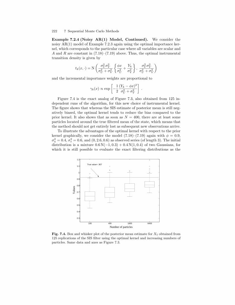
222 7 Sequential Monte Carlo Methods

Example 7.2.4 (Noisy AR(1) Model, Continued). We consider thenoisy AR(1) model of Example 7.2.3 again using the optimal importance ker-nel, which corresponds to the particular case where all variables are scalar andA and R are constant in (7.18)–(7.19) above. Thus, the optimal instrumentaltransition density is given by

tk(x, ·) = N(

σ2Uσ

2V

σ2U + σ2

V

φx

σ2U

+Ykσ2V

,

σ2Uσ

2V

σ2U + σ2

V

)and the incremental importance weights are proportional to

γk(x) ∝ exp[−1

2(Yk − φx)2

σ2U + σ2

V

].

Figure 7.4 is the exact analog of Figure 7.3, also obtained from 125 in-dependent runs of the algorithm, for this new choice of instrumental kernel.The figure shows that whereas the SIS estimate of posterior mean is still neg-atively biased, the optimal kernel tends to reduce the bias compared to theprior kernel. It also shows that as soon as N = 400, there are at least someparticles located around the true filtered mean of the state, which means thatthe method should not get entirely lost as subsequent new observations arrive.

To illustrate the advantages of the optimal kernel with respect to the priorkernel graphically, we consider the model (7.18)–(7.19) again with φ = 0.9,σ2u = 0.4, σ2

v = 0.6, and (0, 2.6, 0.6) as observed series (of length 3). The initialdistribution is a mixture 0.6 N(−1, 0.3) + 0.4 N(1, 0.4) of two Gaussians, forwhich it is still possible to evaluate the exact filtering distributions as the

100 400 1600 6400

0.3

0.4

0.5

0.6

0.7

0.8

0.9

1

1.1

1.2

Val

ues

Number of particles

True value= .907

Fig. 7.4. Box and whisker plot of the posterior mean estimate for X5 obtained from125 replications of the SIS filter using the optimal kernel and increasing numbers ofparticles. Same data and axes as Figure 7.3.

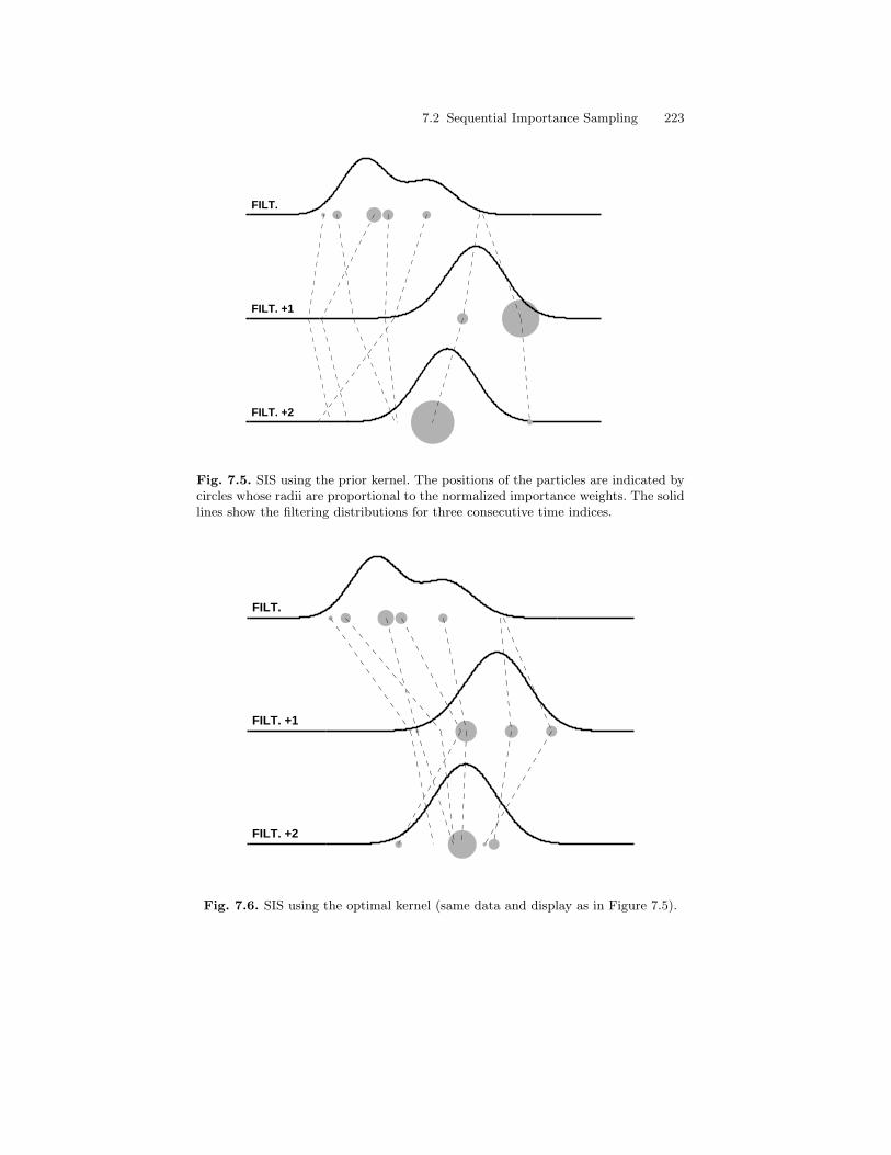
7.2 Sequential Importance Sampling 223

FILT.

FILT. +1

FILT. +2

Fig. 7.5. SIS using the prior kernel. The positions of the particles are indicated bycircles whose radii are proportional to the normalized importance weights. The solidlines show the filtering distributions for three consecutive time indices.

FILT.

FILT. +1

FILT. +2

Fig. 7.6. SIS using the optimal kernel (same data and display as in Figure 7.5).

224 7 Sequential Monte Carlo Methods

mixture of two Kalman filters using, respectively, N(−1, 0.3) and N(1, 0.4) asthe initial distribution of X0. We use only seven particles to allow for an in-terpretable graphical representation. Figures 7.5 and 7.6 show the positions ofthe particles propagated using the prior kernel and the optimal kernel, respec-tively. At time 1, there is a conflict between the prior and the posterior as theobservation does not agree with the particle approximation of the predictivedistribution. With the prior kernel (Figure 7.5), the mass becomes concen-trated on a single particle with several particles lost out in the left tail ofthe distribution with negligible weights. In contrast, in Figure 7.6 most of theparticles stay in high probability regions through the iterations with severaldistinct particles having non-negligible weights. This is precisely because theoptimal kernel “pulls” particles toward regions where the current local likeli-hood gk+1(x) = gk+1(x, Yk) is large, whereas the prior kernel does not.

7.2.2.3 Accept-Reject Algorithm

Because drawing from the optimal kernel Tk is most often not feasible, a firstnatural idea consists in trying the accept-reject method (Algorithm 6.2.1),which is a versatile approach to sampling from general distributions. To sam-ple from the optimal importance kernel Tk(x, ·) defined by (7.15), one needsan instrumental kernel Rk(x, ·) from which it is easy to sample and such thatthere exists M satisfying dQ(x,·)

dRk(x,·) (x′)gk(x′) ≤ M (for all x ∈ X). Note thatbecause it is generally impossible to evaluate the normalizing constant γk ofTk, we must resort here to the unnormalized version of the accept-reject algo-rithm (see Remark 6.2.4). The algorithm consists in generating pairs (ξ, U) ofindependent random variables with ξ ∼ Rk(x, ·) and U uniformly distributedon [0, 1] and accepting ξ if

U ≤ 1M

dQ(x, ·)dRk(x, ·)

(ξ)gk(ξ) .

Recall that the distribution of the number of simulations required is geometricwith parameter

p(x) =∫Q(x, dx′)gk(x′)

M.

The strength of the accept-reject technique is that, using any instrumentalkernel Rk satisfying the domination condition, one can obtain independentsamples from the optimal importance kernel Tk. When the conditional like-lihood of the observation gk(x)—viewed as a function of x—is bounded, onecan for example use the prior kernel Q as the instrumental distribution. Inthat case

dTk(x, ·)dQ(x, ·)

(x′) =gk(x′)∫

gk(u)Q(x, du)≤

supx′∈X gk(x′)∫gk(u)Q(x, du)

.

7.2 Sequential Importance Sampling 225

The algorithm then consists in drawing ξ from the prior kernel Q(x, ·), Uuniformly on [0, 1] and accepting the draw if U ≤ gk(ξ)/ supx∈X gk(x). Theacceptance rate of this algorithm is then given by

p(x) =

∫XQ(x, dx′)gk(x′)

supx′∈X gk(x′).

Unfortunately, it is not always possible to design an importance kernel Rk(x, ·)that is easy to sample from, for which the bound M is indeed finite, and suchthat the acceptance rate p(x) is reasonably large.

7.2.2.4 Local Approximation of the Optimal Importance Kernel

A different option consists in trying to approximate the optimal kernel Tk by asimpler proposal kernel Rk that is handy for simulating. Ideally, Rk should besuch that Rk(x, ·) both has heavier tails than Tk(x, ·) and is close to Tk(x, ·)around its modes, with the aim of keeping the ratio dTk(x,·)

dRk(x,·) (x′) as small aspossible. To do so, authors such as Pitt and Shephard (1999) and Doucetet al. (2000a) suggest to first locate the high-density regions of the optimaldistribution Tk(x, ·) and then use an over-dispersed (that is, with sufficientlyheavy tails) approximation of Tk(x, ·). The first part of this program mostlyapplies to the case where the distribution Tk(x, ·) is known to be unimodalwith a mode that can be located in some way. The overall procedure will needto be repeated N times with x corresponding in turn to each of the currentparticles. Hence the method used to construct the approximation should bereasonably simple if the potential advantages of using a “good” proposal kernelare not to be offset by an unbearable increase in computational cost.

A first remark of interest is that there is a large class of state-space modelsfor which the distribution Tk(x, ·) can effectively be shown to be unimodalusing convexity arguments. In the remainder of this section, we assume thatX = Rd and that the hidden Markov model is fully dominated (in the senseof Definition 2.2.3), denoting by q the transition density function associatedwith the hidden chain. Recall that for a certain form of non-linear state-spacemodels given by (7.18)–(7.19), we were able to derive the optimal kernel andits normalization constant explicitly. Now consider the case where the stateevolves according to (7.18), so that

q(x, x′) ∝ exp[−1

2(x′ −A(x))t

R(c)Rt(x)

−1 (x′ −A(x))],

and g(x, y) is simply constrained to be a log-concave function of its x ar-gument. This of course includes the linear Gaussian observation model con-sidered previously in (7.19) but also many other cases like the non-linearobservation considered below in Example 7.2.5. Then the optimal transitiondensity tuk(x, x′) = (Lk+1/Lk)−1q(x, x′)gk(x′) is also a log-concave function of

226 7 Sequential Monte Carlo Methods

its x′ argument, as its logarithm is the sum of two concave functions (and aconstant term). This implies in particular that x′ 7→ tuk(x, x′) is unimodal andthat its mode may be located using computationally efficient techniques suchas Newton iterations.

The instrumental transition density function is usually chosen from aparametric family rθθ∈Θ of densities indexed by a finite-dimensional pa-rameter θ. An obvious choice is the multivariate Gaussian distribution withmean m and covariance matrix Γ , in which case θ = (µ, Γ ). A better choiceis a multivariate t-distribution with η-degrees of freedom, location m, andscale matrix Γ . Recall that the density of this distribution is proportional torθ(x) ∝ [η+ (x−m)tΓ−1(x−m)](−η+d)/2. The choice η = 1 corresponds to aCauchy distribution. This is a conservative choice that ensures over-dispersion,but if X is high-dimensional, most draws from a multivariate Cauchy mightbe too far away from the mode to reasonably approximate the target distribu-tion. In most situations, values such as η = 4 (three finite moments) are morereasonable, especially if the underlying model does not feature heavy-taileddistributions. Recall also that simulation from the multivariate t-distributionwith η degrees of freedom, location m, and scale Σ can easily be achievedby first drawing from a multivariate Gaussian distribution with mean m andcovariance Γ and then dividing the outcome by the square root of an inde-pendent chi-square draw with η degrees of freedom divided by η.

To choose the parameter θ of the instrumental distribution rθ, one shouldtry to minimize the supremum of the importance function,

minθ∈Θ

supx′∈X

q(x, x′)gk(x′)rθ(x′)

. (7.21)

This is a minimax guarantee by which θ is chosen to minimize an upper boundon the importance weights. Note that if rθ was to be used for sampling fromtk(x, ·) by the accept-reject algorithm, the value of θ for which the minimum isachieved in (7.21) is also the one that would make the acceptance probabilitymaximal (see Section 6.2.1). In practice, solving the optimization problemin (7.21) is often too demanding, and a more generic strategy consists inlocating the mode of x′ 7→ tk(x, x′) by an iterative algorithm and evaluatingthe Hessian of its logarithm at the mode. The parameter θ is then selected inthe following way.

Multivariate normal: fit the mean of the normal distribution to the modeof tk(x, ·) and fit the covariance to minus the inverse of the Hessian oflog t(x, ·) at the mode.

Multivariate t-distribution: fit the location and scale parameters as the meanand covariance parameters in the normal case; the number of degrees offreedom is usually set arbitrarily (and independently of x) based on thearguments discussed above.

We discuss below an important model for which this strategy is successful.

7.2 Sequential Importance Sampling 227

Example 7.2.5 (Stochastic Volatility Model). We return to the stoch-astic volatility model introduced as Example 1.3.13 and considered previouslyin the context of MCMC methods as Example 6.2.16. From the state-spaceequations that define the model,

Xk+1 = φXk + σUk ,

Yk = β exp(Xk/2)Vk ,

we directly obtain

q(x, x′) =1√

2πσ2exp

[− (x′ − φx)2

2σ2

],

gk(x′) =1√

2πβ2exp

[− Y

2k

2β2exp(−x′)− 1

2x′].

Simulating from the optimal transition kernel tk(x, x′) is difficult, but thefunction x′ 7→ log(q(x, x′)gk(x′)) is indeed (strictly) concave. The mode mk(x)of x′ 7→ tk(x, x′) is the unique solution of the non-linear equation

− 1σ2

(x′ − φx) +Y 2k

2β2exp(−x′)− 1

2= 0 , (7.22)

which can be found using Newton iterations. Once at the mode, the (squared)scale σ2

k(x) is set as minus the inverse of the second-order derivative of x′ 7→(log q(x, x′)gk(x′)) evaluated at the mode mk(x). The result is

σ2k(x) =

1σ2

+Y 2k

2β2exp [−mk(x)]

−1

. (7.23)

In this example, a t-distribution with η = 5 degrees of freedom was used, withlocation mk(x) and scale σk(x) obtained as above. The incremental impor-tance weight is then given by

exp[− (x′−φx)2

2σ2 − Y 2k

2β2 exp(−x′)− x′

2

]σ−1k (x)

η + [x′−mk(x)]2

σ2k(x)

−(η+1)/2.

As in the case of Example 6.2.16, the first time index (k = 0) is particular,and it is easily checked that m0(x) is the solution of

−1− φ2

σ2x− 1

2+Y 2

0

2β2exp(−x) = 0 ,

and σ0(x) is given by

σ20(x) =

[1− φ2

σ2+Y 2

0

2β2exp(−m0)

]−1

.

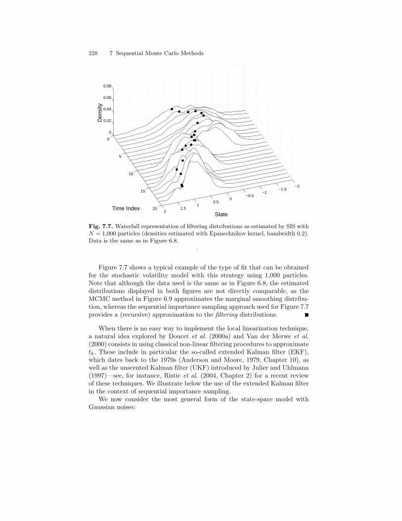
228 7 Sequential Monte Carlo Methods

−2−1.5

−1−0.5

00.5

11.5

2

0

5

10

15

20

0

0.02

0.04

0.06

0.08

StateTime Index

Den

sity

Fig. 7.7. Waterfall representation of filtering distributions as estimated by SIS withN = 1,000 particles (densities estimated with Epanechnikov kernel, bandwidth 0.2).Data is the same as in Figure 6.8.

.

Figure 7.7 shows a typical example of the type of fit that can be obtainedfor the stochastic volatility model with this strategy using 1,000 particles.Note that although the data used is the same as in Figure 6.8, the estimateddistributions displayed in both figures are not directly comparable, as theMCMC method in Figure 6.9 approximates the marginal smoothing distribu-tion, whereas the sequential importance sampling approach used for Figure 7.7provides a (recursive) approximation to the filtering distributions.

When there is no easy way to implement the local linearization technique,a natural idea explored by Doucet et al. (2000a) and Van der Merwe et al.(2000) consists in using classical non-linear filtering procedures to approximatetk. These include in particular the so-called extended Kalman filter (EKF),which dates back to the 1970s (Anderson and Moore, 1979, Chapter 10), aswell as the unscented Kalman filter (UKF) introduced by Julier and Uhlmann(1997)—see, for instance, Ristic et al. (2004, Chapter 2) for a recent reviewof these techniques. We illustrate below the use of the extended Kalman filterin the context of sequential importance sampling.

We now consider the most general form of the state-space model withGaussian noises:

7.2 Sequential Importance Sampling 229

Xk+1 = a(Xk, Uk) , Uk ∼ N(0, I) , (7.24)Yk = b(Xk, Vk) , Vk ∼ N(0, I) , (7.25)

where a, b are vector-valued measurable functions. It is assumed that Ukk≥0

and Vkk≥0 are independent white Gaussian noises. As usual, X0 is as-sumed to be N(0, Σν) distributed and independent of Uk and Vk. Theextended Kalman filter proceeds by approximating the non-linear state-spaceequations (7.24)–(7.25) by a non-linear Gaussian state-space model with linearmeasurement equation. We are then back to a model of the form (7.18)–(7.19)for which the optimal kernel may be determined exactly using Gaussian for-mulas. We will adopt the approximation

Xk ≈ a(Xk−1, 0) +R(Xk−1)Uk−1 , (7.26)Yk ≈ b [a(Xk−1, 0), 0] +B(Xk−1) [Xk − a(Xk−1, 0)] + S(Xk−1)Vk , (7.27)

where

• R(x) is the dx × du matrix of partial derivatives of a(x, u) with respect tou and evaluated at (x, 0),

[R(x)]i,jdef=

∂ [a(x, 0)]i∂uj

for i = 1, . . . , dx and j = 1, . . . , du ;

• B(x) and S(x) are the dy × dx and dy × dv matrices of partial derivativesof b(x, v) with respect to x and v respectively and evaluated at (a(x, 0), 0),

[B(x)]i,j =∂ b [a(x, 0), 0]i

∂xjfor i = 1, . . . , dy and j = 1, . . . , dx ,

[S(x)]i,j =∂ b [a(x, 0), 0]i

∂vjfor i = 1, . . . , dy and j = 1, . . . , dv .

It should be stressed that the measurement equation in (7.27) differsfrom (7.19) in that it depends both on the current state Xk and on the previ-ous one Xk−1. The approximate model specified by (7.26)–(7.27) thus departsfrom the HMM assumptions. On the other hand, when conditioning on thevalue of Xk−1, the structure of both models, (7.18)–(7.19) and (7.26)–(7.27),are exactly similar. Hence the posterior distribution of the state Xk givenXk−1 = x and Yk is a Gaussian distribution with mean mk(x) and covariancematrix Γk(x), which can be evaluated according to

Kk(x) = R(x)Rt(x)Bt(x)[B(x)R(x)Rt(x)Bt(x) + S(x)St(x)

]−1,

mk(x) = a(x, 0) +Kk(x) Yk − b [a(x, 0), 0] ,Γ (x) = [I −Kk(x)B(x)]R(x)Rt(x) .

The Gaussian distribution with mean mk(x) and covariance Γk(x) may thenbe used as a proxy for the optimal transition kernel Tk(x, ·). To improve

230 7 Sequential Monte Carlo Methods

the robustness of the method, it is safe to increase the variance, that is, touse cΓk(x) as the simulation variance, where c is a scalar larger than one. Aperhaps more recommendable option consists in using as previously a proposaldistribution with tails heavier than the Gaussian, for instance, a multivariatet-distribution with location mk(x), scale Γk(x), and four or five degrees offreedom.

Example 7.2.6 (Growth Model). We consider the univariate growthmodel discussed by Kitagawa (1987) and Polson et al. (1992) given, in state-space form, by

Xk = ak−1(Xk−1) + σuUk−1 , Uk ∼ N(0, 1) , (7.28)

Yk = bX2k + σvVk , Vk ∼ N(0, 1) , (7.29)

where Ukk≥0 and Vkk≥0 are independent white Gaussian noise processesand

ak−1(x) = α0x+ α1x

1 + x2+ α2 cos [1.2(k − 1)] (7.30)

with α0 = 0.5, α1 = 25, α2 = 8, b = 0.05, and σ2v = 1 (the value of σ2

u willbe discussed below). The initial state is known deterministically and set toX0 = 0.1. This model is non-linear both in the state and in the measurementequation. Note that the form of the likelihood adds an interesting twist to theproblem: whenever Yk ≤ 0, the conditional likelihood function

gk(x) def= g(x;Yk) ∝ exp[− b2

2σ2v

(x2 − Yk/b

)2]is unimodal and symmetric about 0; when Yk > 0 however, the likelihood gkis symmetric about 0 with two modes located at ±(Yk/b)1/2.

The EKF approximation to the optimal transition kernel is a Gaussiandistribution with mean mk(x) and variance Γk(x) given by

Kk(x) = 2σ2ubak−1(x)

[4σ2

ub2a2k−1(x) + σ2

v

]−1,

mk(x) = ak−1(x) +Kk(x)[Yk − ba2

k−1(x)],

Γk(x) =σ2vσ

2u

4σ2ub

2a2k−1(x) + σ2

v

.

In Figure 7.8, the optimal kernel, the EKF approximation to the optimalkernel, and the prior kernel for two different values of the state variance arecompared. This figure corresponds to the time index one, and Y1 is set to 6(recall that the initial state X0 is equal to 0.1). In the case where σ2

u = 1 (leftplot in Figure 7.8), the prior distribution of the state, N(a0(X0), σ2

u), turnsout to be more informative (more peaky, less diffuse) than the conditionallikelihood g1. In other words, the observed Y1 does not carry a lot of informa-tion about the state X1, compared to the information provided by X0; this

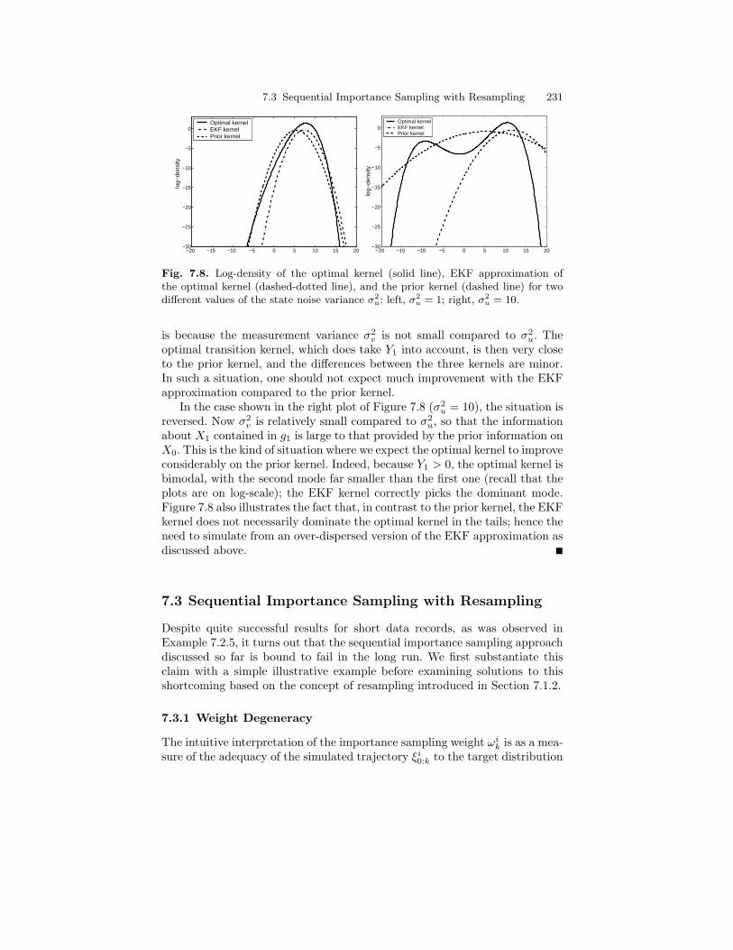
7.3 Sequential Importance Sampling with Resampling 231

−20 −15 −10 −5 0 5 10 15 20−30

−25

−20

−15

−10

−5

0Optimal kernelEKF kernelPrior kernel

log−

dens

ity

−20 −15 −10 −5 0 5 10 15 20−30

−25

−20

−15

−10

−5

0

log−

dens

ity

Optimal kernelEKF kernelPrior kernel

Fig. 7.8. Log-density of the optimal kernel (solid line), EKF approximation ofthe optimal kernel (dashed-dotted line), and the prior kernel (dashed line) for twodifferent values of the state noise variance σ2

u: left, σ2u = 1; right, σ2

u = 10.

is because the measurement variance σ2v is not small compared to σ2

u. Theoptimal transition kernel, which does take Y1 into account, is then very closeto the prior kernel, and the differences between the three kernels are minor.In such a situation, one should not expect much improvement with the EKFapproximation compared to the prior kernel.

In the case shown in the right plot of Figure 7.8 (σ2u = 10), the situation is

reversed. Now σ2v is relatively small compared to σ2

u, so that the informationabout X1 contained in g1 is large to that provided by the prior information onX0. This is the kind of situation where we expect the optimal kernel to improveconsiderably on the prior kernel. Indeed, because Y1 > 0, the optimal kernel isbimodal, with the second mode far smaller than the first one (recall that theplots are on log-scale); the EKF kernel correctly picks the dominant mode.Figure 7.8 also illustrates the fact that, in contrast to the prior kernel, the EKFkernel does not necessarily dominate the optimal kernel in the tails; hence theneed to simulate from an over-dispersed version of the EKF approximation asdiscussed above.

7.3 Sequential Importance Sampling with Resampling

Despite quite successful results for short data records, as was observed inExample 7.2.5, it turns out that the sequential importance sampling approachdiscussed so far is bound to fail in the long run. We first substantiate thisclaim with a simple illustrative example before examining solutions to thisshortcoming based on the concept of resampling introduced in Section 7.1.2.

7.3.1 Weight Degeneracy

The intuitive interpretation of the importance sampling weight ωik is as a mea-sure of the adequacy of the simulated trajectory ξi0:k to the target distribution

232 7 Sequential Monte Carlo Methods

φ0:k|n. A small importance weight implies that the trajectory is drawn far fromthe main body of the posterior distribution φ0:k|n and will contribute onlymoderately to the importance sampling estimates of the form (7.11). Indeed,a particle such that the associated weight ωik is orders of magnitude smallerthan the sum

∑Ni=1 ω

ik is practically ineffective. If there are too many inef-

fective particles, the particle approximation becomes both computationallyand statistically inefficient: most of the computing effort is put on updatingparticles and weights that do not contribute significantly to the estimator;the variance of the resulting estimator will not reflect the large number ofterms in the sum but only the small number of particles with non-negligiblenormalized weights.

Unfortunately, the situation described above is the rule rather than theexception, as the importance weights will (almost always) degenerate as thetime index k increases, with most of the normalized importance weightsωik/

∑Nj=1 ω

jk close to 0 except for a few ones. We consider below the case

of i.i.d. models for which it is possible to show using simple arguments thatthe large sample variance of the importance sampling estimate can only in-crease with the time index k.

Example 7.3.1 (Weight Degeneracy in the I.I.D. Case). The simplestcase of application of the sequential importance sampling technique is when µis a probability distribution on (X,X ) and the sequence of target distributionscorresponds to the product distributions, that is, the sequence of distributionson (Xk+1,X⊗(k+1)) defined recursively by µ0 = µ and µk = µk−1 ⊗ µ, fork ≥ 1. Let ν be another probability distribution on (X,X ) and assume that µis absolutely continuous with respect to ν and that∫ [

dµ

dν(x)]2

ν(dx) <∞ . (7.31)

Finally, let f be a bounded measurable function that is not (µ-a.s.) constantsuch that its variance under µ, µ(f2)− µ2(f), is strictly positive.

Consider the sequential importance sampling estimate given by

µISk,N (f) =

N∑i=1

f(ξik)∏kl=0

dµdν (ξik)∑N

j=1

∏kl=0

dµdν (ξjk)

, (7.32)

where the random variables ξjl , l = 1, . . . , k, j = 1, . . . , N are i.i.d. with com-mon distribution ν. As discussed in Section 7.2, the unnormalized importanceweights may be computed recursively and hence (7.32) really corresponds toan estimator of the form (7.11) in the particular case of a function fk thatdepends on the last component only. This is of course a rather convoluted andvery inefficient way of constructing an estimate of µ(f) but still constitutesa valid instance of the sequential importance sampling approach (in a veryparticular case).

7.3 Sequential Importance Sampling with Resampling 233

Now let k be fixed and write

N1/2µISk,N (f)− µ(f)

=N−1/2

∑Ni=1

∏kl=0

f(ξik)− µ(f)

dµdν (ξil )

N−1∑Ni=1

∏kl=0

dµdν (ξil )

.

(7.33)Because

E

[k∏l=0

dµ

dν(ξil )

]= 1 ,

the weak law of large numbers implies that the denominator of the right-handside of (7.33) converges to 1 in probability as N increases. Likewise, under(7.31), the central limit theorem shows that the numerator of the right-handside of (7.33) converges in distribution to the normal N(0, σ2

k(f)) distribution,where

σ2k(f) = E

k∏l=0

[f(ξ1

k)− µ(f)]2 dµdν

(ξ1l )

2 (7.34)

=

[∫ (dµ

dν(x))2

ν(dx)

]k ∫ [dµ

dν(x)]2

[f(x)− µ(f)]2 ν(dx) .

Slutsky’s lemma then implies that (7.33) also converges in distribution to thesame N(0, σ2

k(f)) limit as N grows. Now Jensen’s inequality implies that

1 =[∫

dµ

dν(x)ν(dx)

]2

≤∫ [

dµ

dν(x)]2

ν(dx) ,

with equality if and only if µ = ν. Therefore, if µ 6= ν, the asymptotic varianceσ2k(f) grows exponentially with the iteration index k for all functions f such

that∫ [dµ

dν(x)]2

[f(x)− µ(f)]2 ν(dx) =∫dµ

dν(x) [f(x)− µ(f)]2 µ(dx) 6= 0 .

Because µ is absolutely continuous with respect to ν, µx ∈ X : dµ/dν(x) =0 = 0 and the last integral is null if and only if f has zero variance under µ.

Thus in the i.i.d. case, the asymptotic variance of the importance samplingestimate (7.32) increases exponentially with the time index k as soon as theproposal and target differ (except for constant functions).

It is more difficult to characterize the degeneracy of the weights for gen-eral target and instrumental distributions. There have been some limited at-tempts to study more formally this phenomenon in some specific scenarios.In particular, Del Moral and Jacod (2001) have shown the degeneracy of thesequential importance sampling estimator of the posterior mean in Gaussianlinear models when the instrumental kernel is the prior kernel. Such results

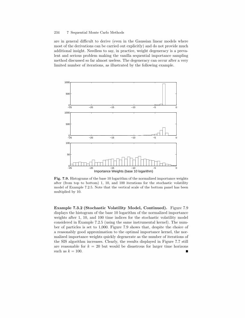
234 7 Sequential Monte Carlo Methods

are in general difficult to derive (even in the Gaussian linear models wheremost of the derivations can be carried out explicitly) and do not provide muchadditional insight. Needless to say, in practice, weight degeneracy is a preva-lent and serious problem making the vanilla sequential importance samplingmethod discussed so far almost useless. The degeneracy can occur after a verylimited number of iterations, as illustrated by the following example.

−25 −20 −15 −10 −5 00

500

1000

−25 −20 −15 −10 −5 00

500

1000

−25 −20 −15 −10 −5 00

50

100

Importance Weights (base 10 logarithm)

Fig. 7.9. Histograms of the base 10 logarithm of the normalized importance weightsafter (from top to bottom) 1, 10, and 100 iterations for the stochastic volatilitymodel of Example 7.2.5. Note that the vertical scale of the bottom panel has beenmultiplied by 10.

Example 7.3.2 (Stochastic Volatility Model, Continued). Figure 7.9displays the histogram of the base 10 logarithm of the normalized importanceweights after 1, 10, and 100 time indices for the stochastic volatility modelconsidered in Example 7.2.5 (using the same instrumental kernel). The num-ber of particles is set to 1,000. Figure 7.9 shows that, despite the choice ofa reasonably good approximation to the optimal importance kernel, the nor-malized importance weights quickly degenerate as the number of iterations ofthe SIS algorithm increases. Clearly, the results displayed in Figure 7.7 stillare reasonable for k = 20 but would be disastrous for larger time horizonssuch as k = 100.

7.3 Sequential Importance Sampling with Resampling 235

Because the weight degeneracy phenomenon is so detrimental, it is of greatpractical significance to set up tests that can detect this phenomenon. A simplecriterion is the coefficient of variation of the normalized weights used by Konget al. (1994), which is defined by

CVN =

1N

N∑i=1

(N

ωi∑Nj=1 ω

j− 1

)21/2

. (7.35)

The coefficient of variation is minimal when the normalized weights are allequal to 1/N , and then CVN = 0. The maximal value of CVN is

√N − 1,

which corresponds to one of the normalized weights being one and all othersbeing null. Therefore, the coefficient of variation is often interpreted as ameasure of the number of ineffective particles (those that do not significantlycontribute to the estimate). A related criterion with a simpler interpretationis the so-called effective sample size Neff (Liu, 1996), defined as

Neff =

N∑i=1

(ωi∑Nj=1 ω

j

)2−1

, (7.36)

which varies between 1 (all weights null but one) and N (equal weights). It isstraightforward to verify the relation

Neff =N

1 + CV2N

.

Some additional insights and heuristics about the coefficient of variation aregiven by Liu and Chen (1995).

Yet another possible measure of the weight imbalance is the Shannon en-tropy of the importance weights,

Ent = −N∑i=1

ωi∑Nj=1 ω

jlog2

(ωi∑Nj=1 ω

j

). (7.37)

When all the normalized importance weights are null except for one of them,the entropy is null. On the contrary, if all the weights are equal to 1/N , thenthe entropy is maximal and equal to log2N .

Example 7.3.3 (Stochastic Volatility Model, Continued). Figure 7.10displays the coefficient of variation (left) and Shannon entropy (right) as afunction of the time index k under the same conditions as for Figure 7.9,that is, for the stochastic volatility model of 7.2.5. The figure shows that thedistribution of the weights steadily degenerates: the coefficient of variationincreases and the entropy of the importance weights decreases. After 100 iter-ations, there are less than 50 particles (out 1,000) significantly contributing to

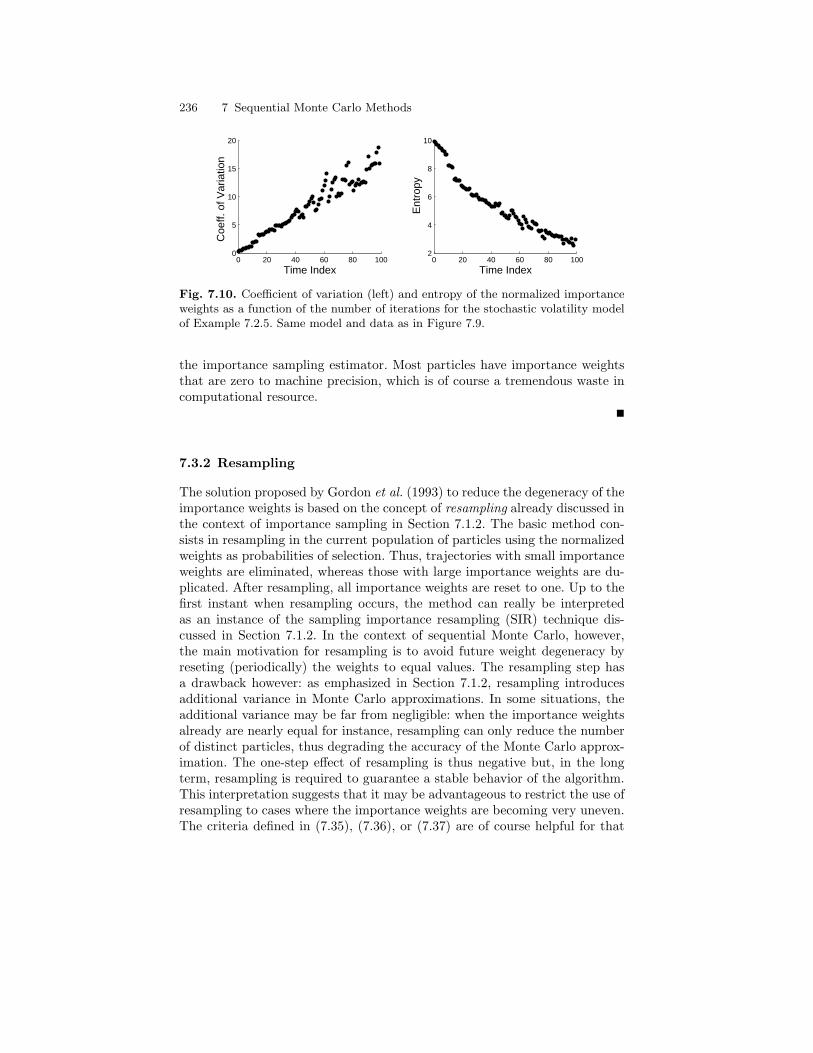
236 7 Sequential Monte Carlo Methods

0 20 40 60 80 1000

5

10

15

20

Time Index

Coe

ff. o

f Var

iatio

n

0 20 40 60 80 1002

4

6

8

10

Time Index

Ent

ropy

Fig. 7.10. Coefficient of variation (left) and entropy of the normalized importanceweights as a function of the number of iterations for the stochastic volatility modelof Example 7.2.5. Same model and data as in Figure 7.9.

the importance sampling estimator. Most particles have importance weightsthat are zero to machine precision, which is of course a tremendous waste incomputational resource.

7.3.2 Resampling

The solution proposed by Gordon et al. (1993) to reduce the degeneracy of theimportance weights is based on the concept of resampling already discussed inthe context of importance sampling in Section 7.1.2. The basic method con-sists in resampling in the current population of particles using the normalizedweights as probabilities of selection. Thus, trajectories with small importanceweights are eliminated, whereas those with large importance weights are du-plicated. After resampling, all importance weights are reset to one. Up to thefirst instant when resampling occurs, the method can really be interpretedas an instance of the sampling importance resampling (SIR) technique dis-cussed in Section 7.1.2. In the context of sequential Monte Carlo, however,the main motivation for resampling is to avoid future weight degeneracy byreseting (periodically) the weights to equal values. The resampling step hasa drawback however: as emphasized in Section 7.1.2, resampling introducesadditional variance in Monte Carlo approximations. In some situations, theadditional variance may be far from negligible: when the importance weightsalready are nearly equal for instance, resampling can only reduce the numberof distinct particles, thus degrading the accuracy of the Monte Carlo approx-imation. The one-step effect of resampling is thus negative but, in the longterm, resampling is required to guarantee a stable behavior of the algorithm.This interpretation suggests that it may be advantageous to restrict the use ofresampling to cases where the importance weights are becoming very uneven.The criteria defined in (7.35), (7.36), or (7.37) are of course helpful for that

7.3 Sequential Importance Sampling with Resampling 237

purpose. The resulting algorithm, which is generally known under the name ofsequential importance sampling with resampling (SISR), is summarized below.

Algorithm 7.3.4 (SISR: Sequential Importance Sampling with Re-sampling). Initialize the particles as in Algorithm 7.2.2, optionally applying theresampling step below. For subsequent time indices k ≥ 0, do the following.

Sampling:• Draw (ξ1

k+1, . . . , ξNk+1) conditionally independently given ξj0:k , j =

1, . . . , N from the instrumental kernel: ξik+1 ∼ Rk(ξik, ·), i = 1, . . . , N .• Compute the updated importance weights

ωik+1 = ωikgk+1(ξik+1)dQ(ξik, ·)dRk(ξik, ·)

(ξik+1) , i = 1, . . . , N .

Resampling (Optional):• Draw, conditionally independently given (ξi0:k, ξ

jk+1), i, j = 1, . . . , N,

the multinomial trial (I1k+1, . . . I

Nk+1) with probabilities of success

ω1k+1∑N

j ωjk+1

, . . . ,ωNk+1∑Nj ω

jk+1

.

• Reset the importance weights ωik+1 to a constant value for i = 1, . . . , N .If resampling is not applied, set for i = 1, . . . , N , Iik+1 = i.

Trajectory update: for i = 1, . . . , N ,

ξi0:k+1 =(ξIik+10:k , ξ

Iik+1k+1

). (7.38)

As discussed previously the resampling step in the algorithm above maybe used systematically (for all indices k), but it is often preferable to performresampling from time to time only. Usually, resampling is either used system-atically but at a lower rate (for one index out of m, where m is fixed) or atrandom instants based on the values of the coefficient of variation or the en-tropy criteria defined in (7.35) and (7.37), respectively. Note that in additionto arguments based on the variance of the Monte Carlo approximation, thereis usually also a computational incentive for limiting the use of resampling;indeed, except in models where the evaluation of the incremental weights iscostly (think of large-dimensional multivariate observations for instance), thecomputational cost of the resampling step is not negligible. Both Sections 7.4.1and 7.4.2 discuss several implementations and variants of the resampling stepthat may render the latter argument less pregnant.

The term particle filter is often used to refer to Algorithm 7.3.4 althoughthe terminology SISR is preferable, as particle filtering is sometimes also usedmore generically for any sequential Monte Carlo method. Gordon et al. (1993)actually proposed a specific instance of Algorithm 7.3.4 in which resampling

238 7 Sequential Monte Carlo Methods

is done systematically at each step and the instrumental kernel is chosen asthe prior kernel Rk = Q. This particular algorithm, commonly known as thebootstrap filter , is most often very easy to implement because it only involvessimulating from the transition kernel Q of the hidden chain and evaluation ofthe conditional likelihood function g.

There is of course a whole range of variants and refinements of Algo-rithm 7.3.4, many of which will be covered in some detail in the next chapter.A simple remark though is that, as in the case of the simplest SIR methoddiscussed in Section 7.1.2, it is possible to resample N times from a larger pop-ulation of M intermediate samples. In practice, it means that Algorithm 7.3.4should be modified as follows at indices k for which resampling is to be applied.

SIS: For i = 1, . . . , N , draw α candidates ξi,1k+1, . . . , ξi,αk+1 from each proposal

distribution Rk(ξik, ·).Resampling: Draw (N1,1

k+1, . . . , N1,αk+1, . . . , NN,1

k+1, . . . , NN,αk+1 ) from the multi-

nomial distribution with parameter N and probabilities

ωi,jk+1∑Nl=1

∑αm=1 ω

l,mk+1

for i = 1, . . . , N , j = 1, . . . , α .

Hence, while this form of resampling keeps the number of particles fixed andequal to N after resampling, the intermediate population (before resampling)has size M = α × N . Although obviously heavier to implement, the use ofα larger than one may be advantageous in some models. In particular, wewill show in Chapter 9 that using α larger than one effectively reduces thevariance associated with the resampling operation in a proportion that maybe significant.

Remark 7.3.5 (Marginal Interpretation of SIS and SISR). Both Al-gorithms 7.2.2 and 7.3.4 have been introduced as methods to simulate wholetrajectories ξi0:k1≤i≤N that approximate the joint smoothing distributionφ0:k|k. This was done quite easily in the case of sequential importance sam-pling (Algorithm 7.2.2), as the trajectories are simply extended independentlyof one another as new samples arrive. When using resampling however, theprocess is more involved because it becomes necessary to duplicate or discardsome trajectories according to (7.38).

This presentation of the SIS and SISR methods has been adopted becauseit is the most natural way to introduce sequential Monte Carlo methods.It does not mean that, when implementing the SISR algorithm, storing thewhole trajectories is required. Neither do we claim that for large k, the ap-proximation of the complete joint distribution φ0:k|k provided by the particletrajectories ξi0:k1≤i≤N is accurate (this point will be discussed in detail inSection 8.3). Most often, Algorithm 7.3.4 is implemented storing only thecurrent generation of particles ξik1≤i≤N , and (7.38) simplifies to

ξik+1 = ξIik+1k+1 i = 1, . . . , N .

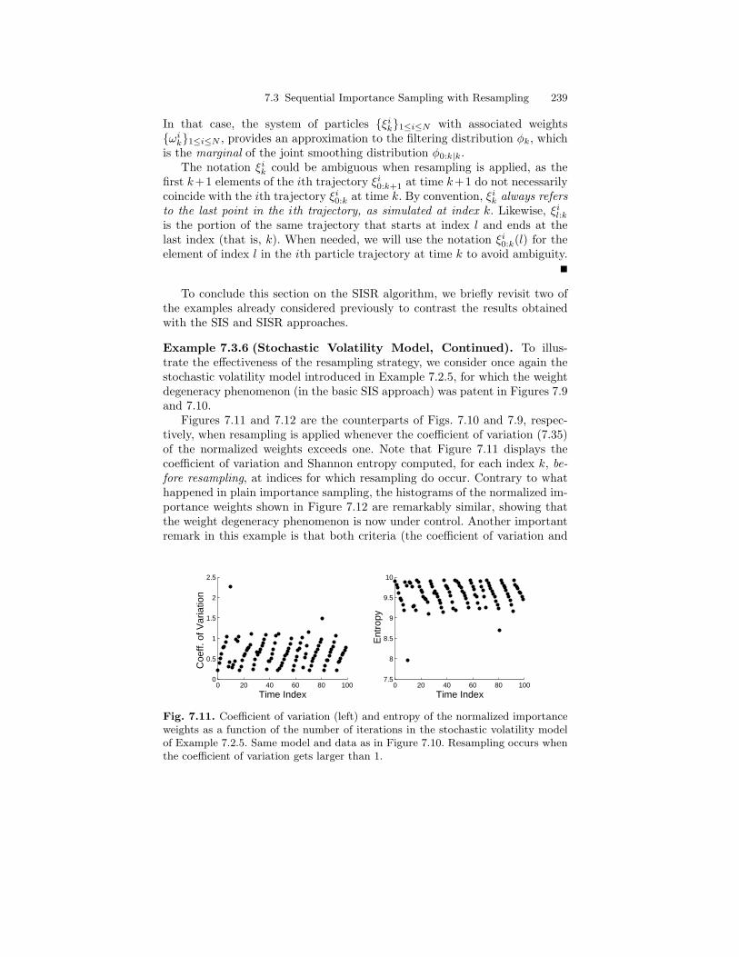
7.3 Sequential Importance Sampling with Resampling 239

In that case, the system of particles ξik1≤i≤N with associated weightsωik1≤i≤N , provides an approximation to the filtering distribution φk, whichis the marginal of the joint smoothing distribution φ0:k|k.

The notation ξik could be ambiguous when resampling is applied, as thefirst k+1 elements of the ith trajectory ξi0:k+1 at time k+1 do not necessarilycoincide with the ith trajectory ξi0:k at time k. By convention, ξik always refersto the last point in the ith trajectory, as simulated at index k. Likewise, ξil:kis the portion of the same trajectory that starts at index l and ends at thelast index (that is, k). When needed, we will use the notation ξi0:k(l) for theelement of index l in the ith particle trajectory at time k to avoid ambiguity.

To conclude this section on the SISR algorithm, we briefly revisit two ofthe examples already considered previously to contrast the results obtainedwith the SIS and SISR approaches.

Example 7.3.6 (Stochastic Volatility Model, Continued). To illus-trate the effectiveness of the resampling strategy, we consider once again thestochastic volatility model introduced in Example 7.2.5, for which the weightdegeneracy phenomenon (in the basic SIS approach) was patent in Figures 7.9and 7.10.

Figures 7.11 and 7.12 are the counterparts of Figs. 7.10 and 7.9, respec-tively, when resampling is applied whenever the coefficient of variation (7.35)of the normalized weights exceeds one. Note that Figure 7.11 displays thecoefficient of variation and Shannon entropy computed, for each index k, be-fore resampling, at indices for which resampling do occur. Contrary to whathappened in plain importance sampling, the histograms of the normalized im-portance weights shown in Figure 7.12 are remarkably similar, showing thatthe weight degeneracy phenomenon is now under control. Another importantremark in this example is that both criteria (the coefficient of variation and

0 20 40 60 80 1000

0.5

1

1.5

2

2.5

Time Index

Coe

ff. o

f Var

iatio

n

0 20 40 60 80 1007.5

8

8.5

9

9.5

10

Time Index

Ent

ropy

Fig. 7.11. Coefficient of variation (left) and entropy of the normalized importanceweights as a function of the number of iterations in the stochastic volatility modelof Example 7.2.5. Same model and data as in Figure 7.10. Resampling occurs whenthe coefficient of variation gets larger than 1.

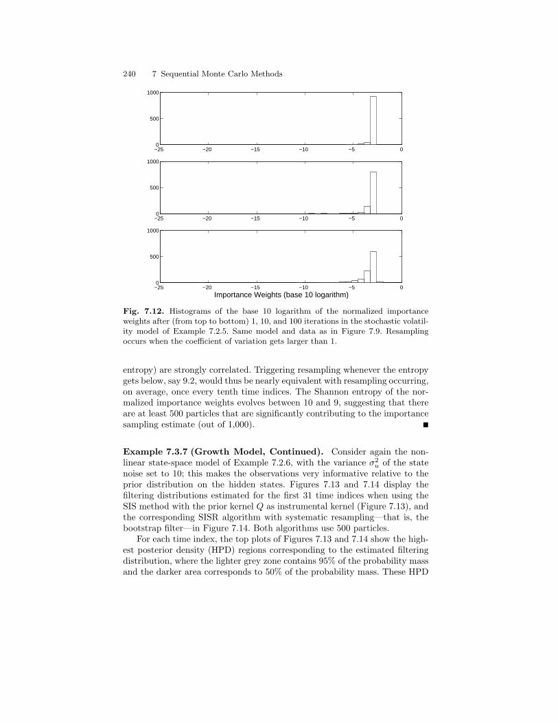
240 7 Sequential Monte Carlo Methods

−25 −20 −15 −10 −5 00

500

1000

−25 −20 −15 −10 −5 00

500

1000

−25 −20 −15 −10 −5 00

500

1000

Importance Weights (base 10 logarithm)

Fig. 7.12. Histograms of the base 10 logarithm of the normalized importanceweights after (from top to bottom) 1, 10, and 100 iterations in the stochastic volatil-ity model of Example 7.2.5. Same model and data as in Figure 7.9. Resamplingoccurs when the coefficient of variation gets larger than 1.

entropy) are strongly correlated. Triggering resampling whenever the entropygets below, say 9.2, would thus be nearly equivalent with resampling occurring,on average, once every tenth time indices. The Shannon entropy of the nor-malized importance weights evolves between 10 and 9, suggesting that thereare at least 500 particles that are significantly contributing to the importancesampling estimate (out of 1,000).

Example 7.3.7 (Growth Model, Continued). Consider again the non-linear state-space model of Example 7.2.6, with the variance σ2

u of the statenoise set to 10; this makes the observations very informative relative to theprior distribution on the hidden states. Figures 7.13 and 7.14 display thefiltering distributions estimated for the first 31 time indices when using theSIS method with the prior kernel Q as instrumental kernel (Figure 7.13), andthe corresponding SISR algorithm with systematic resampling—that is, thebootstrap filter—in Figure 7.14. Both algorithms use 500 particles.

For each time index, the top plots of Figures 7.13 and 7.14 show the high-est posterior density (HPD) regions corresponding to the estimated filteringdistribution, where the lighter grey zone contains 95% of the probability massand the darker area corresponds to 50% of the probability mass. These HPD

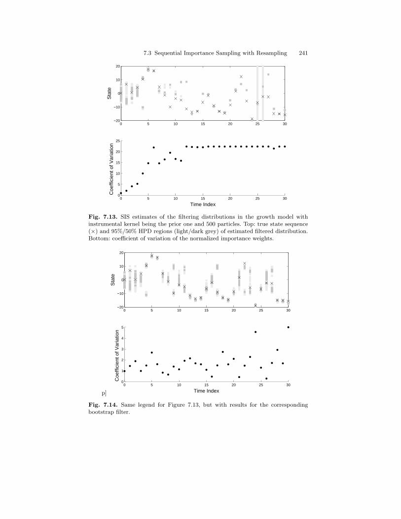
7.3 Sequential Importance Sampling with Resampling 241

0 5 10 15 20 25 300

5

10

15

20

25

Time Index

Coe

ffici

ent o

f Var

iatio

n

0 5 10 15 20 25 30−20

−10

0

10

20

Sta

te

Fig. 7.13. SIS estimates of the filtering distributions in the growth model withinstrumental kernel being the prior one and 500 particles. Top: true state sequence(×) and 95%/50% HPD regions (light/dark grey) of estimated filtered distribution.Bottom: coefficient of variation of the normalized importance weights.

p]

0 5 10 15 20 25 300

1

2

3

4

5

Time Index

Coe

ffici

ent o

f Var

iatio

n

0 5 10 15 20 25 30−20

−10

0

10

20

Sta

te

Fig. 7.14. Same legend for Figure 7.13, but with results for the correspondingbootstrap filter.

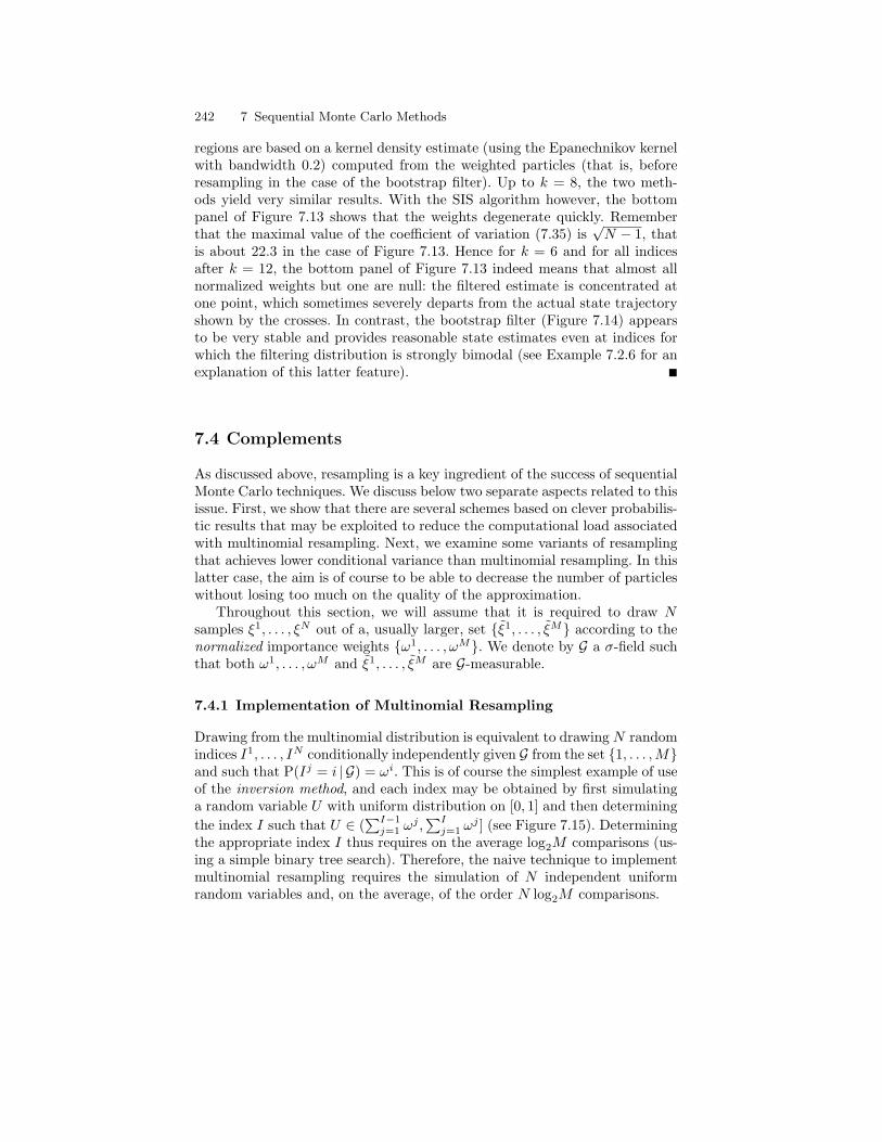
242 7 Sequential Monte Carlo Methods

regions are based on a kernel density estimate (using the Epanechnikov kernelwith bandwidth 0.2) computed from the weighted particles (that is, beforeresampling in the case of the bootstrap filter). Up to k = 8, the two meth-ods yield very similar results. With the SIS algorithm however, the bottompanel of Figure 7.13 shows that the weights degenerate quickly. Rememberthat the maximal value of the coefficient of variation (7.35) is

√N − 1, that

is about 22.3 in the case of Figure 7.13. Hence for k = 6 and for all indicesafter k = 12, the bottom panel of Figure 7.13 indeed means that almost allnormalized weights but one are null: the filtered estimate is concentrated atone point, which sometimes severely departs from the actual state trajectoryshown by the crosses. In contrast, the bootstrap filter (Figure 7.14) appearsto be very stable and provides reasonable state estimates even at indices forwhich the filtering distribution is strongly bimodal (see Example 7.2.6 for anexplanation of this latter feature).

7.4 Complements

As discussed above, resampling is a key ingredient of the success of sequentialMonte Carlo techniques. We discuss below two separate aspects related to thisissue. First, we show that there are several schemes based on clever probabilis-tic results that may be exploited to reduce the computational load associatedwith multinomial resampling. Next, we examine some variants of resamplingthat achieves lower conditional variance than multinomial resampling. In thislatter case, the aim is of course to be able to decrease the number of particleswithout losing too much on the quality of the approximation.

Throughout this section, we will assume that it is required to draw Nsamples ξ1, . . . , ξN out of a, usually larger, set ξ1, . . . , ξM according to thenormalized importance weights ω1, . . . , ωM. We denote by G a σ-field suchthat both ω1, . . . , ωM and ξ1, . . . , ξM are G-measurable.

7.4.1 Implementation of Multinomial Resampling

Drawing from the multinomial distribution is equivalent to drawing N randomindices I1, . . . , IN conditionally independently given G from the set 1, . . . ,Mand such that P(Ij = i | G) = ωi. This is of course the simplest example of useof the inversion method, and each index may be obtained by first simulatinga random variable U with uniform distribution on [0, 1] and then determiningthe index I such that U ∈ (

∑I−1j=1 ω

j ,∑Ij=1 ω

j ] (see Figure 7.15). Determiningthe appropriate index I thus requires on the average log2M comparisons (us-ing a simple binary tree search). Therefore, the naive technique to implementmultinomial resampling requires the simulation of N independent uniformrandom variables and, on the average, of the order N log2M comparisons.

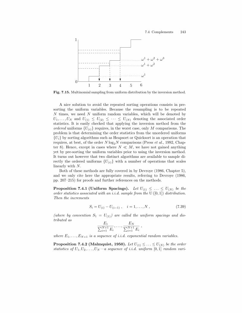
7.4 Complements 243

1

1 2 43 65

ω1

ω1 + ω

2

ω1 + ω

2 + ω3

0

Fig. 7.15. Multinomial sampling from uniform distribution by the inversion method.

A nice solution to avoid the repeated sorting operations consists in pre-sorting the uniform variables. Because the resampling is to be repeatedN times, we need N uniform random variables, which will be denoted byU1, . . . , UN and U(1) ≤ U(2) ≤ · · · ≤ U(N) denoting the associated orderstatistics. It is easily checked that applying the inversion method from theordered uniforms U(i) requires, in the worst case, only M comparisons. Theproblem is that determining the order statistics from the unordered uniformsUi by sorting algorithms such as Heapsort or Quicksort is an operation thatrequires, at best, of the order N log2N comparisons (Press et al., 1992, Chap-ter 8). Hence, except in cases where N M , we have not gained anythingyet by pre-sorting the uniform variables prior to using the inversion method.It turns out however that two distinct algorithms are available to sample di-rectly the ordered uniforms U(i) with a number of operations that scaleslinearly with N .

Both of these methods are fully covered in by Devroye (1986, Chapter 5),and we only cite here the appropriate results, referring to Devroye (1986,pp. 207–215) for proofs and further references on the methods.

Proposition 7.4.1 (Uniform Spacings). Let U(1) ≤ . . . ≤ U(N) be theorder statistics associated with an i.i.d. sample from the U ([0, 1]) distribution.Then the increments

Si = U(i) − U(i−1) , i = 1, . . . , N , (7.39)

(where by convention S1 = U(1)) are called the uniform spacings and dis-tributed as

E1∑N+1i=1 Ei

, . . . ,EN∑N+1i=1 Ei

,

where E1, . . . , EN+1 is a sequence of i.i.d. exponential random variables.

Proposition 7.4.2 (Malmquist, 1950). Let U(1) ≤ . . . ≤ U(N) be the orderstatistics of U1, U2, . . . , UN—a sequence of i.i.d. uniform [0, 1] random vari-

244 7 Sequential Monte Carlo Methods

ables. Then U1/NN , U1/N

N U1/(N−1)N−1 , . . . , U1/N

N U1/(N−1)N−1 · · ·U1/1

1 is distributedas U(N), . . . , U(1).

The two sampling algorithms associated with these probabilistic resultsmay be summarized as follows.

Algorithm 7.4.3 (After Proposition 7.4.1).

For i = 1, . . . , N + 1: Simulate Ui ∼ U ([0, 1]) and set Ei = − logUi.Set G =

∑N+1i=1 Ei and U(1) = E1/G.

For i = 2, . . . , n: U(i) = U(i−1) + Ei/G.

Algorithm 7.4.4 (After Proposition 7.4.2).

Generate VN ∼ U ([0, 1]) and set U(N) = V1/NN .

For i = N − 1 down to 1: Generate Vi ∼ U ([0, 1]) and set U(i) = V1/ii U(i+1).

Note that Devroye (1986) also discusses a third, slightly more complicatedalgorithm—the bucket sort method of Devroye and Klincsek (1981)—whichalso has an expected computation time of order N . Using any of these meth-ods, the computational cost of multinomial resampling scales only linearly inN and M , which makes the method practicable even when a large number ofparticles is used.

7.4.2 Alternatives to Multinomial Resampling

Instead of using the multinomial sampling scheme, it is also possible to use adifferent resampling (or reallocation) scheme. For i = 1, . . . ,M , denote by N i

the number of times the ith element ξi is selected. A resampling scheme willbe said to be unbiased with respect to G if

M∑i=1

N i = N , (7.40)

E[N i∣∣G] = Nωi, i = 1, . . . ,M . (7.41)

We focus here on resampling techniques that keep the number of particlesconstant (see for instance Crisan et al., 1999, for unbiased sampling with arandom number of particles). There are many different conditions under whicha resampling scheme is unbiased. The simplest unbiased scheme is multinomialresampling, for which (N1, . . . , NM ), conditionally on G, has the multinomi-mal distribution Mult(N,ω1, . . . , ωN ). Because I1, . . . , IM are conditionallyi.i.d. given G, it is easy to evaluate the conditional variance in the multino-mial resampling scheme:

7.4 Complements 245

Var

[1N

N∑i=1

f(ξIi

)

∣∣∣∣∣G]

=1N

M∑i=1

ωi

f(ξi)−M∑j=1

ωjf(ξj)

2

=1N

M∑i=1

ωif2(ξi)−

[M∑i=1

ωif(ξi)

]2 . (7.42)

A sensible objective is to try to construct resampling schemes for which theconditional variance Var(

∑Ni=1

Ni

N f(ξi) | G) is as small as possible and, in par-ticular, smaller than (7.42), preferably for any choice of the function f .

7.4.2.1 Residual Resampling

Residual resampling, or remainder resampling, is mentioned by Whitley (1994)(see also Liu and Chen, 1998) as a simple means to decrease the varianceincurred by the sampling step. In this scheme, for i = 1, . . . ,M we set

N i =⌊Nωi

⌋+ N i , (7.43)

where N1, . . . , NM are distributed, conditionally on G, according to the multi-nomial distribution Mult(N −R, ω1, . . . , ωN ) with R =

∑Mi=1bNωic and

ωi =Nωi − bNωic

N −R, i = 1, . . . ,M . (7.44)

This scheme is obviously unbiased with respect to G. Equivalently, for anymeasurable function f , the residual sampling estimator is

1N

N∑i=1

f(ξi) =M∑i=1

bNωicN

f(ξi) +1N

N−R∑i=1

f(ξJi

) , (7.45)

where J1, . . . , JN−R are conditionally independent given G with distributionP(J i = k | G) = ωk for i = 1, . . . , N−R and k = 1, . . . ,M . Because the residualresampling estimator is the sum of one term that, given G, is deterministicand one term that involves conditionally i.i.d. labels, the variance of residualresampling is given by

1N2

Var

[N−R∑i=1

f(ξJi

)

∣∣∣∣∣G]

=N −RN2

Var[f(ξJ

1)∣∣∣G] (7.46)

=(N −R)N2

M∑i=1

ωi

f(ξi)−M∑j=1

ωjf(ξj)

2

=1N

M∑i=1

ωif2(ξi)−M∑i=1

bNωicN2

f2(ξi)− N −RN2

M∑i=1

ωif(ξi)

2

.

246 7 Sequential Monte Carlo Methods

Residual sampling dominates multinomial sampling also in the sense of havingsmaller conditional variance. Indeed, first write

M∑i=1

ωif(ξi) =M∑i=1

bNωicN

f(ξi) +N −RN

M∑i=1

ωif(ξi) .

Then note that the sum of the M numbers bNωic/N plus (N −R)/N equalsone, whence this sequence of M + 1 numbers can be viewed as a probabilitydistribution. Thus Jensen’s inequality applied to the square of the right-handside of the above display yields

M∑i=1

ωif(ξi)

2

≤M∑i=1

bNωicN

f2(ξi) +N −RN

M∑i=1

ωif(ξi)

2

.

Combining with (7.46) and (7.42), this shows that the conditional variance ofresidual sampling is always smaller than that of multinomial sampling.

7.4.2.2 Stratified Resampling

The inversion method for sampling a multinomial sequence of trials mapsuniform (0, 1) random variables U1, . . . , UN into indices I1, . . . , IN through adeterministic function. For any function f ,

N∑i=1

f(ξIi

) =N∑i=1

Φf (U i) ,

where the function Φf (which depends on both f and ξi) is defined, for anyu ∈ (0, 1], by

Φf (u) def= f(ξI(u)), I(u) =M∑i=1

i1(∑i−1j=1 ω

j ,∑ij=1 ω

j ](u) . (7.47)

Note that, by construction,∫ 1

0Φf (u) du =

∑Mi=1 ω

if(ξi). To reduce the con-ditional variance of

∑Ni=1 f(ξI

i

), we may change the way in which the sampleU1, . . . , UN is drawn. A possible solution, commonly used in survey sampling,is based on stratification (see Kitagawa, 1996, and Fearnhead, 1998, Section5.3, for discussion of the method in the context of particle filtering). Theinterval (0, 1] is partitioned into different strata, assumed for simplicity tobe intervals (0, 1] = (0, 1/N ] ∪ (1/N, 2/N ] ∪ · · · ∪ (N − 1/N, 1]. More gen-eral partitions could have been considered as well; in particular, the numberof partitions does not have to equal N , and the interval lengths could bemade dependent on the ωi. One then draws a sample U1, . . . , UN condition-ally independently given G from the distribution U i ∼ U ((i− 1 /N, i/N ])

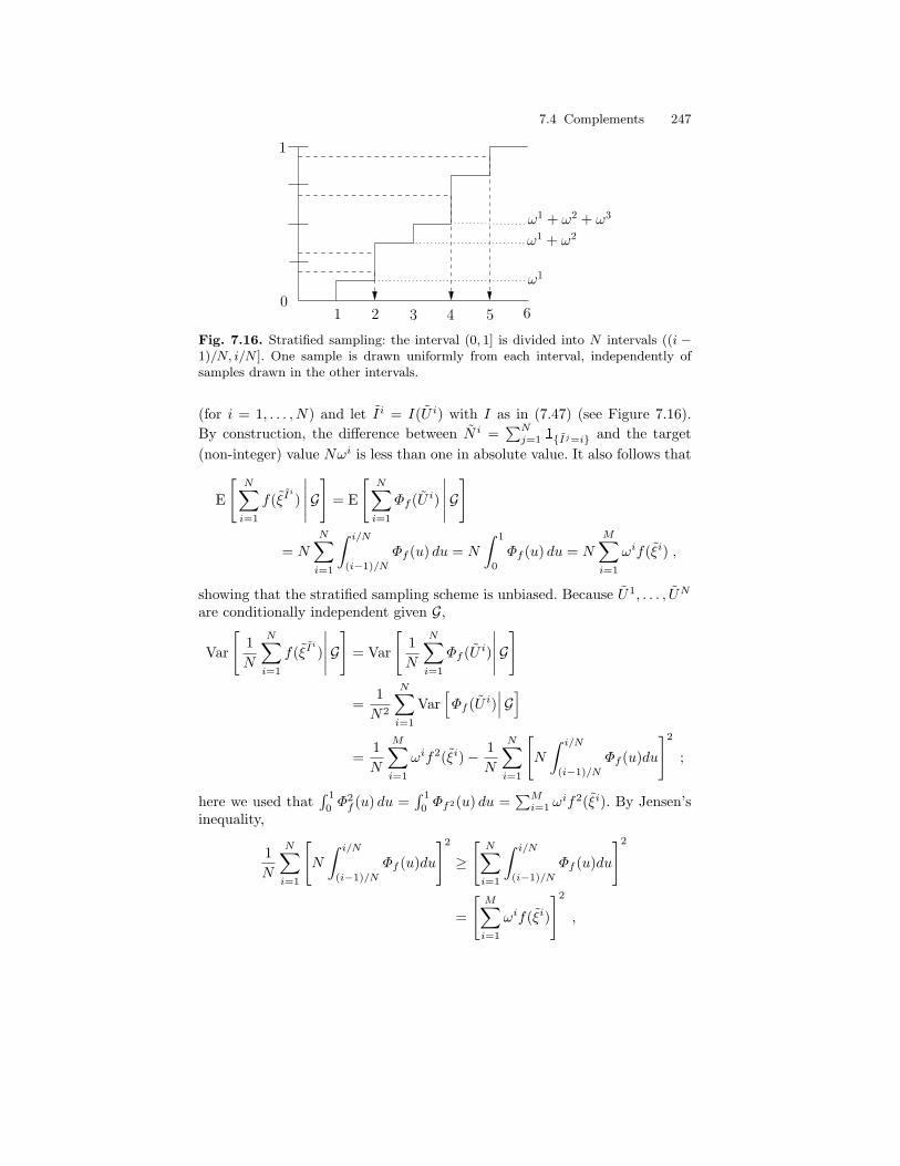
7.4 Complements 247

1

1 2 43 65

ω1

ω1 + ω

2

ω1 + ω

2 + ω3

0

Fig. 7.16. Stratified sampling: the interval (0, 1] is divided into N intervals ((i −1)/N, i/N ]. One sample is drawn uniformly from each interval, independently ofsamples drawn in the other intervals.

(for i = 1, . . . , N) and let Ii = I(U i) with I as in (7.47) (see Figure 7.16).By construction, the difference between N i =

∑Nj=1 1Ij=i and the target

(non-integer) value Nωi is less than one in absolute value. It also follows that

E

[N∑i=1

f(ξIi

)

∣∣∣∣∣G]

= E

[N∑i=1

Φf (U i)

∣∣∣∣∣G]

= N

N∑i=1

∫ i/N

(i−1)/N

Φf (u) du = N

∫ 1

0

Φf (u) du = N

M∑i=1

ωif(ξi) ,

showing that the stratified sampling scheme is unbiased. Because U1, . . . , UN

are conditionally independent given G,

Var

[1N

N∑i=1

f(ξIi

)

∣∣∣∣∣G]

= Var

[1N

N∑i=1

Φf (U i)

∣∣∣∣∣G]

=1N2

N∑i=1

Var[Φf (U i)

∣∣∣G]

=1N

M∑i=1

ωif2(ξi)− 1N

N∑i=1

[N

∫ i/N

(i−1)/N

Φf (u)du

]2

;

here we used that∫ 1

0Φ2f (u) du =

∫ 1

0Φf2(u) du =

∑Mi=1 ω

if2(ξi). By Jensen’sinequality,

1N

N∑i=1

[N

∫ i/N

(i−1)/N

Φf (u)du

]2

≥

[N∑i=1

∫ i/N

(i−1)/N

Φf (u)du

]2

=

[M∑i=1

ωif(ξi)

]2

,

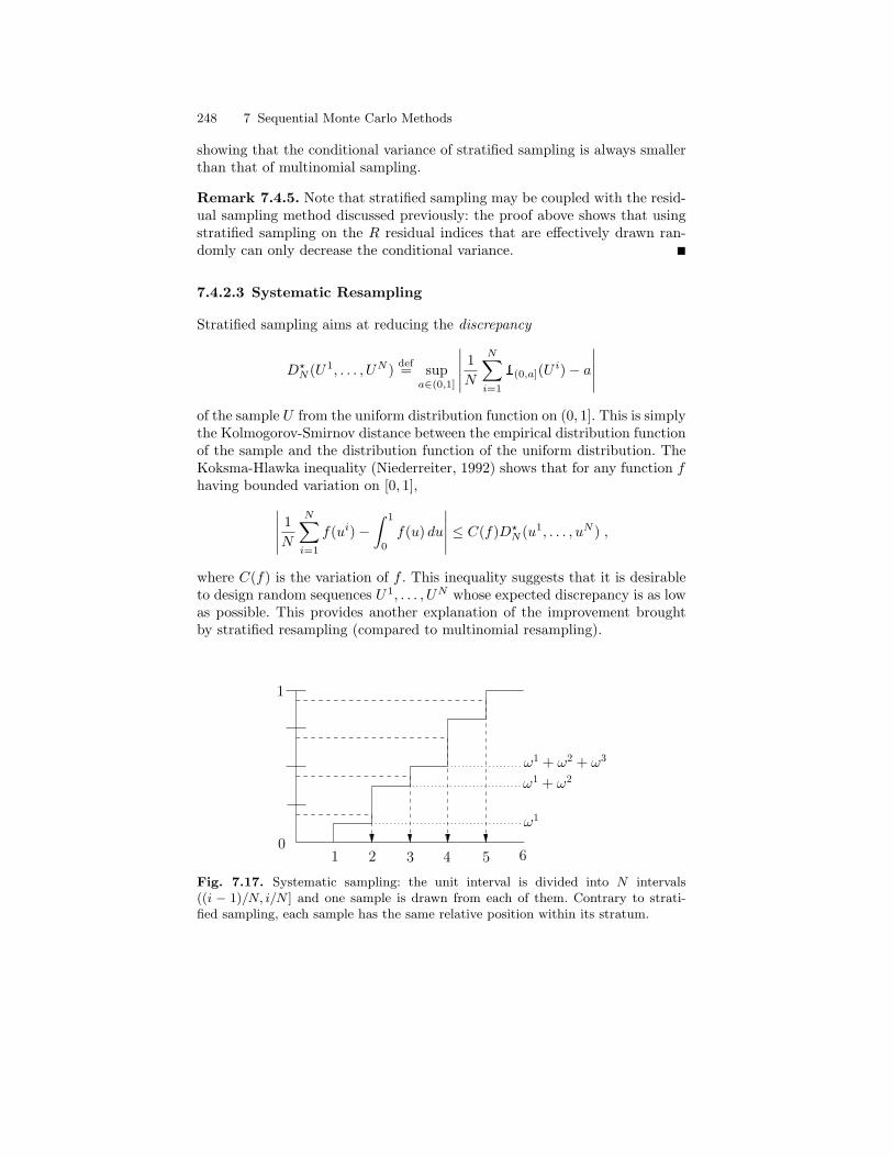
248 7 Sequential Monte Carlo Methods

showing that the conditional variance of stratified sampling is always smallerthan that of multinomial sampling.

Remark 7.4.5. Note that stratified sampling may be coupled with the resid-ual sampling method discussed previously: the proof above shows that usingstratified sampling on the R residual indices that are effectively drawn ran-domly can only decrease the conditional variance.

7.4.2.3 Systematic Resampling

Stratified sampling aims at reducing the discrepancy

D?N (U1, . . . , UN ) def= sup

a∈(0,1]

∣∣∣∣∣ 1N

N∑i=1

1(0,a](U i)− a

∣∣∣∣∣of the sample U from the uniform distribution function on (0, 1]. This is simplythe Kolmogorov-Smirnov distance between the empirical distribution functionof the sample and the distribution function of the uniform distribution. TheKoksma-Hlawka inequality (Niederreiter, 1992) shows that for any function fhaving bounded variation on [0, 1],∣∣∣∣∣ 1

N

N∑i=1

f(ui)−∫ 1

0

f(u) du

∣∣∣∣∣ ≤ C(f)D?N (u1, . . . , uN ) ,

where C(f) is the variation of f . This inequality suggests that it is desirableto design random sequences U1, . . . , UN whose expected discrepancy is as lowas possible. This provides another explanation of the improvement broughtby stratified resampling (compared to multinomial resampling).

1

1 2 43 65

ω1

ω1 + ω

2

ω1 + ω

2 + ω3

0

Fig. 7.17. Systematic sampling: the unit interval is divided into N intervals((i − 1)/N, i/N ] and one sample is drawn from each of them. Contrary to strati-fied sampling, each sample has the same relative position within its stratum.

7.4 Complements 249

Pursuing in this direction, it makes sense to look for sequences with evensmaller average discrepancy. One such sequence is U i = U + (i− 1)/N , whereU is drawn from a uniform U((0, 1/N ]) distribution. In survey sampling, thismethod is known as systematic sampling. It was introduced in the particlefilter literature by Carpenter et al. (1999) but is mentioned by Whitley (1994)under the name of universal sampling. The interval (0, 1] is still divided intoN sub-intervals (i− 1/N, i/N ] and one sample is taken from each of them,as in stratified sampling. However, the samples are no longer independent, asthey have the same relative position within each stratum (see Figure 7.17).This sampling scheme is obviously still unbiased. Because the samples are nottaken independently across strata, it is however not possible to obtain simpleformulas for the conditional variance (Kunsch, 2003). It is often conjecturedthat the conditional variance of systematic resampling is always lower thanthat of multinomial resampling. This is not correct, as demonstrated by thefollowing example.

Example 7.4.6. Consider the case where the initial population of particlesξi1≤i≤N is composed of the interleaved repetition of only two distinct valuesx0 and x1, with identical multiplicities (assuming N to be even). In otherwords,

ξi1≤i≤N = x0, x1, x0, x1, . . . , x0, x1 .

We denote by 2ω/N the common value of the normalized weight ωi associatedto the N/2 particles ξi that satisfy ξi = x1, so that the remaining ones (whichare such that ξi = x0) share a common weight of 2(1 − ω)/N . Without lossof generality, we assume that 1/2 ≤ ω < 1 and that the function of interest fis such that f(x0) = 0 and f(x1) = F .

Under multinomial resampling, (7.42) shows that the conditional varianceof the estimate N−1

∑Ni=1 f(ξi) is given by

Var

[1N

N∑i=1

f(ξimult)

∣∣∣∣∣G]

=1N

(1− ω)ωF 2 . (7.48)

Because the value 2ω/N is assumed to be larger than 1/N , it is easilychecked that systematic resampling deterministically sets N/2 of the ξi to beequal to x1. Depending on the draw of the initial shift, all the N/2 remainingparticles are either set to x1, with probability 2ω−1, or to x0, with probability2(1−ω). Hence the variance is that of a single Bernoulli draw scaled by N/2,that is,

Var

[1N

N∑i=1

f(ξisyst)

∣∣∣∣∣G]

= (ω − 1/2)(1− ω)F 2 .

Note that in this case, the conditional variance of systematic resampling is notonly larger than (7.48) for most values of ω (except when ω is very close to1/2), but it does not even decrease to zero as N grows! Clearly, this observa-tion is very dependent on the order in which the initial population of particles

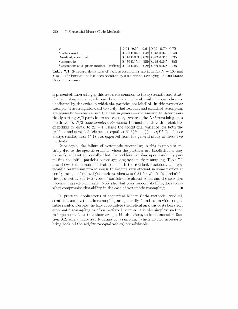
250 7 Sequential Monte Carlo Methods

ω 0.51 0.55 0.6 0.65 0.70 0.75

Multinomial 0.050 0.049 0.049 0.048 0.046 0.043Residual, stratified 0.010 0.021 0.028 0.032 0.035 0.035Systematic 0.070 0.150 0.200 0.229 0.245 0.250Systematic with prior random shuffling 0.023 0.030 0.029 0.029 0.028 0.025

Table 7.1. Standard deviations of various resampling methods for N = 100 andF = 1. The bottom line has been obtained by simulations, averaging 100,000 MonteCarlo replications.

is presented. Interestingly, this feature is common to the systematic and strat-ified sampling schemes, whereas the multinomial and residual approaches areunaffected by the order in which the particles are labelled. In this particularexample, it is straightforward to verify that residual and stratified resamplingare equivalent—which is not the case in general—and amount to determinis-tically setting N/2 particles to the value x1, whereas the N/2 remaining onesare drawn by N/2 conditionally independent Bernoulli trials with probabilityof picking x1 equal to 2ω − 1. Hence the conditional variance, for both theresidual and stratified schemes, is equal to N−1(2ω− 1)(1−ω)F 2. It is hencealways smaller than (7.48), as expected from the general study of these twomethods.

Once again, the failure of systematic resampling in this example is en-tirely due to the specific order in which the particles are labelled: it is easyto verify, at least empirically, that the problem vanishes upon randomly per-muting the initial particles before applying systematic resampling. Table 7.1also shows that a common feature of both the residual, stratified, and sys-tematic resampling procedures is to become very efficient in some particularconfigurations of the weights such as when ω = 0.51 for which the probabili-ties of selecting the two types of particles are almost equal and the selectionbecomes quasi-deterministic. Note also that prior random shuffling does some-what compromise this ability in the case of systematic resampling.

In practical applications of sequential Monte Carlo methods, residual,stratified, and systematic resampling are generally found to provide compa-rable results. Despite the lack of complete theoretical analysis of its behavior,systematic resampling is often preferred because it is the simplest methodto implement. Note that there are specific situations, to be discussed in Sec-tion 8.2, where more subtle forms of resampling (which do not necessarilybring back all the weights to equal values) are advisable.

8

Advanced Topics in Sequential Monte Carlo

This chapter deals with three disconnected topics that correspond to variantsand extensions of the sequential Monte Carlo framework introduced in theprevious chapter. Remember that we have already examined in Section 7.2a first and very important degree of freedom in the application of sequentialMonte Carlo methods, namely the choice of the instrumental kernel Rk usedto simulate the trajectories of the particles. We now consider solutions thatdepart, more or less significantly, from the sequential importance samplingwith resampling (SISR) method of Algorithm 7.3.4.

The first section covers a far-reaching revision of the principles behind theSISR algorithm in which sequential Monte Carlo is interpreted as a repeatedsampling task. This reinterpretation suggests several other sequential MonteCarlo schemes that differ, sometimes significantly, from the SISR approach.Section 8.2 reviews methods that exploit the specific hierarchical structurefound in some hidden Markov models, and in particular in conditionally Gaus-sian linear state-space models (CGLSSMs). The algorithms to be consideredthere combine the sequential simulation approach presented in the previouschapter with the Kalman filtering recursion discussed in Chapter 5. Finally,Section 8.3 discusses the use of sequential Monte Carlo methods for approxi-mating smoothed quantities of the form introduced in Section 4.1.

8.1 Alternatives to SISR

We first present a reinterpretation of the objectives of the sequential impor-tance sampling with resampling (SISR) algorithm in Section 7.3. This newinterpretation suggests a whole range of different approaches that combinesmore closely the sampling (trajectory update) and resampling (weight reset)operators involved in the SISR algorithm.

In the basic SISR approach (Algorithm 7.3.4), we expect that after a re-sampling step, say at index k, the particle trajectories ξ1

0:k, . . . , ξN0:k approx-

imately form an i.i.d. sample of size N from the distribution φ0:k|k. We will

252 8 Advanced Topics in SMC

discuss more precisely in Chapter 9 the degree to which this assertion is cor-rect but assume for the moment that the general intuition is justifiable. Evenin the absence of resampling at index k, in which case the weights ω1

k, . . . , ωNk

are not identical, the expectation of any function fk ∈ Fb

(Xk+1

)under φ0:k|k

may be approximated, following (7.11), by

N∑i=1

ωik∑Nj=1 ω

jk

fk(ξi0:k) .

This behavior may indeed be adopted as a general principle for sequentialMonte Carlo techniques, considering that a valid algorithm is such that it isrecursive and guarantees that the weighted empirical distribution,

φ0:k|k =N∑i=1

ωik∑Nj=1 ω

jk

δξi0:k, (8.1)

is a consistent approximation to φ0:k|k, in some suitable sense, as the numberN of particles increases (the symbol δ denotes Dirac measures).

The particular feature of the sequence of target distributions encounteredin the HMM filtering application is the relatively simple recursive form recalledby (7.7):

φ0:k+1|k+1(fk+1) =∫· · ·∫fk+1(x0:k+1)φ0:k|k(dx0:k)T u

k (xk, dxk+1) ,

for all functions fk+1 ∈ Fb

(Xk+2

), where T u

k is the (unnormalized) kerneldefined in (7.8). This relation may be rewritten replacing T u

k by its normalizedversion Tk defined in (7.15), the so-called optimal importance kernel, to obtain

φ0:k+1|k+1(fk+1) =∫· · ·∫fk+1(x0:k+1)φ0:k|k(dx0:k)

× LkLk+1

γk(xk)Tk(xk, dxk+1) , (8.2)

where γk is the normalizing function defined in (7.17). Because the likelihoodsLk and Lk+1 are precisely the type of quantities that are non-evaluable incontexts where sequential Monte Carlo is useful, it is preferable to rewrite (8.2)in the equivalent auto-normalized form

φ0:k+1|k+1(fk+1) =

∫·· ·∫fk+1(x0:k+1)φ0:k|k(dx0:k)γk(xk)Tk(xk, dxk+1)∫

·· ·∫φ0:k|k(dx0:k)γk(xk)

.

(8.3)A natural idea in the context of sequential Monte Carlo is to plug the

approximate empirical distribution defined in (8.1) into the recursive updateformula (8.3), which yields

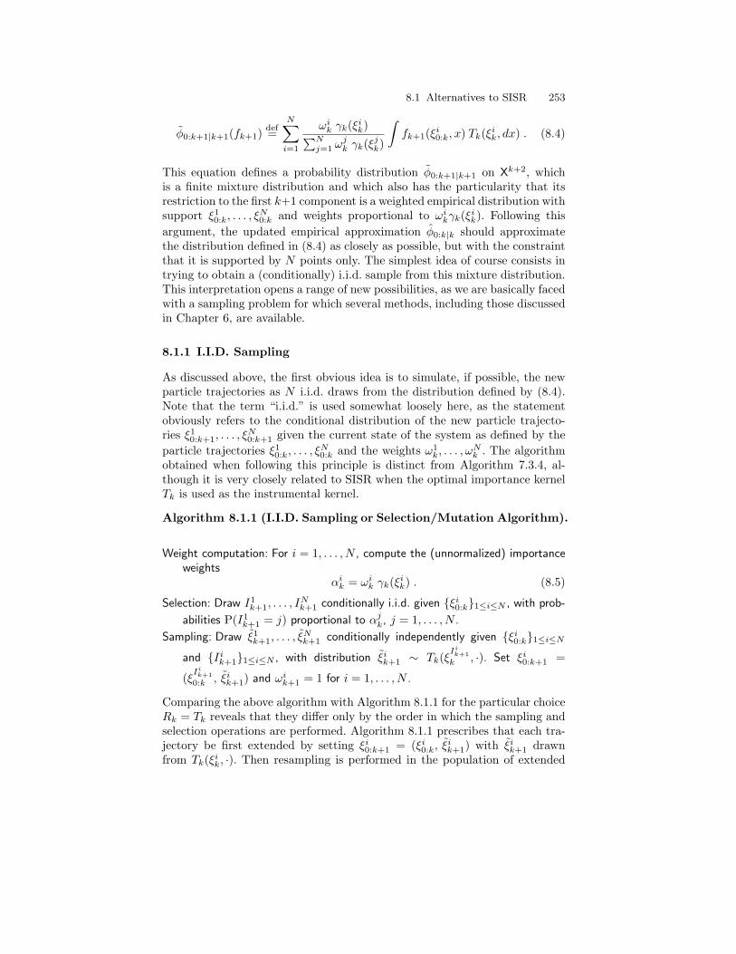
8.1 Alternatives to SISR 253

φ0:k+1|k+1(fk+1) def=N∑i=1

ωik γk(ξik)∑Nj=1 ω

jk γk(ξjk)

∫fk+1(ξi0:k, x) Tk(ξik, dx) . (8.4)

This equation defines a probability distribution φ0:k+1|k+1 on Xk+2, whichis a finite mixture distribution and which also has the particularity that itsrestriction to the first k+1 component is a weighted empirical distribution withsupport ξ1

0:k, . . . , ξN0:k and weights proportional to ωikγk(ξik). Following this

argument, the updated empirical approximation φ0:k|k should approximatethe distribution defined in (8.4) as closely as possible, but with the constraintthat it is supported by N points only. The simplest idea of course consists intrying to obtain a (conditionally) i.i.d. sample from this mixture distribution.This interpretation opens a range of new possibilities, as we are basically facedwith a sampling problem for which several methods, including those discussedin Chapter 6, are available.

8.1.1 I.I.D. Sampling

As discussed above, the first obvious idea is to simulate, if possible, the newparticle trajectories as N i.i.d. draws from the distribution defined by (8.4).Note that the term “i.i.d.” is used somewhat loosely here, as the statementobviously refers to the conditional distribution of the new particle trajecto-ries ξ1

0:k+1, . . . , ξN0:k+1 given the current state of the system as defined by the

particle trajectories ξ10:k, . . . , ξ

N0:k and the weights ω1

k, . . . , ωNk . The algorithm

obtained when following this principle is distinct from Algorithm 7.3.4, al-though it is very closely related to SISR when the optimal importance kernelTk is used as the instrumental kernel.

Algorithm 8.1.1 (I.I.D. Sampling or Selection/Mutation Algorithm).

Weight computation: For i = 1, . . . , N , compute the (unnormalized) importanceweights

αik = ωik γk(ξik) . (8.5)

Selection: Draw I1k+1, . . . , I

Nk+1 conditionally i.i.d. given ξi0:k1≤i≤N , with prob-

abilities P(I1k+1 = j) proportional to αjk, j = 1, . . . , N .

Sampling: Draw ξ1k+1, . . . , ξ

Nk+1 conditionally independently given ξi0:k1≤i≤N

and Iik+11≤i≤N , with distribution ξik+1 ∼ Tk(ξIik+1k , ·). Set ξi0:k+1 =

(ξIik+10:k , ξik+1) and ωik+1 = 1 for i = 1, . . . , N .

Comparing the above algorithm with Algorithm 8.1.1 for the particular choiceRk = Tk reveals that they differ only by the order in which the sampling andselection operations are performed. Algorithm 8.1.1 prescribes that each tra-jectory be first extended by setting ξi0:k+1 = (ξi0:k, ξ

ik+1) with ξik+1 drawn

from Tk(ξik, ·). Then resampling is performed in the population of extended

254 8 Advanced Topics in SMC

trajectories, based on weights given by (8.5) when Rk = Tk. In contrast, Algo-rithm 8.1.1 first selects the trajectories based on the weights αik and then sim-ulates an independent extension for each selected trajectory. This is of coursepossible only because the optimal importance kernel Tk is used as instrumen-tal kernel, rendering the incremental weights independent of the position ofthe particle at index k + 1 and thus allowing for early selection. Intuitively,Algorithm 8.1.1 is preferable because it does not simply duplicate trajectorieswith high weights but rather selects the most promising trajectories at indexk using independent extensions (at index k + 1) for each selected trajectory.Following the terminology in use in genetic algorithms1, Algorithm 8.1.1 is aselection/mutation algorithm, whereas the SISR approach is based on muta-tion/selection. Recall that the latter is more general, as it does not require thatthe optimal kernel Tk be used, although we shall see later, in Section 8.1.2,that the i.i.d. sampling approach can be modified to allow for general instru-mental kernels.

Remark 8.1.2. In Chapter 7 as well as in the exposition above, we consid-ered that the quantity of interest is the joint smoothing measure φ0:k|k. Itis important however to understand that this focus on the joint smoothingmeasure φ0:k|k is unessential as all the algorithms presented so far only relyon the recursive structure observed in (8.4). Of course, in the case of thejoint smoothing measure φ0:k|k, the kernel Tk and the function γk that appearin (8.4) have a specific form given by (7.15) and (7.17):∫

f(x′) γk(x)Tk(x, dx′) =∫f(x′) gk+1(x′)Q(x, dx′) (8.6)

for functions f ∈ Fb (X), where γk(x) equals the above expression evaluatedfor f = 1. However, any of the sequential Monte Carlo algorithms discussed sofar can be used for generic choices of the kernel Tk and the function γk providedthe expression for the incremental weights is suitably modified. The core ofSMC techniques is thus the structure observed in (8.4), whose connection withthe methods exposed here is worked out in detail in the recent book by DelMoral (2004).

As an example, recall from Chapter 3 that the distribution φ0:k|k−1 differsfrom φ0:k−1|k−1 only by an application of the prior (or state transition) kernelQ and hence satisfies a recursion similar to (8.4) with the kernel Tk and thefunction γk replaced by Q and gk, respectively:

φ0:k+1|k(fk+1) =

∫·· ·∫fk+1(x0:k+1)φ0:k|k−1(dx0:k)gk(xk)Q(xk, dxk+1)∫

·· ·∫φ0:k|k−1(dx0:k)gk(xk)

,

(8.7)1Genetic algorithms (see, e.g., Whitley, 1994) have much in common with se-

quential Monte Carlo methods. Their purpose is different however, with an emphasison optimization rather than, as for SMC, simulation. Both fields do share a lot ofcommon terminology.

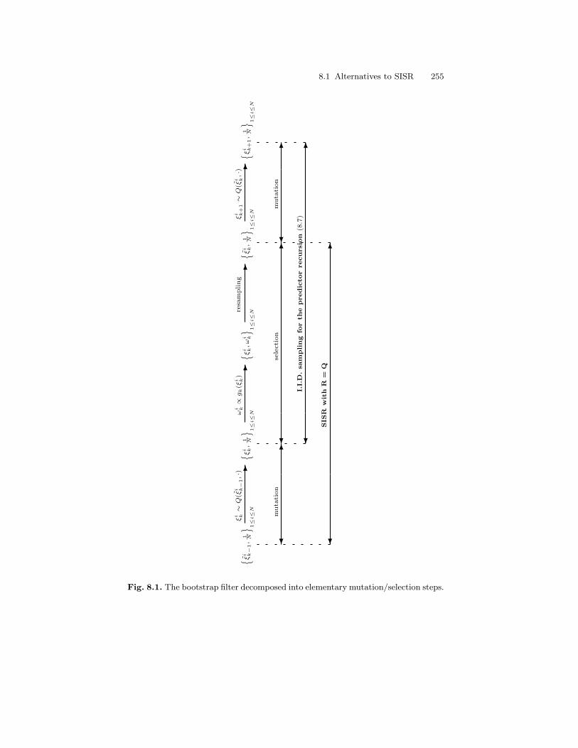
8.1 Alternatives to SISR 255

ξi k−1,

1 N

1≤i≤N

-ξi k∼Q

(ξi k−

1,·)

ξi k,

1 N

1≤i≤N

-ωi k∝gk(ξi k)

ξi k,ωi k

1≤i≤N

-re

sam

pling

ξi k,

1 N

1≤i≤N

-ξi k+

1∼Q

(ξi k,·)

ξi k+1,

1 N

1≤i≤N

-

muta

tion

-

sele

cti

on

-

muta

tion

-

I.I.D

.sam

pling

for

the

predic

tor

recursio

n(8

.7)

-

SIS

Rw

ith

R=

Q

Fig. 8.1. The bootstrap filter decomposed into elementary mutation/selection steps.

256 8 Advanced Topics in SMC

where the denominator could be written more compactly as φk|k−1(gk). Therecursive update formula obtained for the (joint) predictive distribution ismuch simpler than (8.4), as (8.7) features the prior kernel Q—from whichwe generally assume that sampling is feasible—and the conditional likeli-hood function gk—whose analytical expression is known. In particular, it isstraightforward to apply Algorithm 8.1.1 in this case by selecting with weightsgk(ξ1

k), . . . , gk(ξNk ) and mutating the selected particles using the kernel Q. Thisis obviously equivalent to the bootstrap filter (Algorithm 7.3.4 with Q as theinstrumental kernel) viewed at a different stage: just after the selection stepfor Algorithm 7.3.4 and just after the mutation step for Algorithm 8.1.1 ap-plied to the predictive distribution (see Figure 8.1 for an illustration). Theprevious interpretation however suggests that the bootstrap filter operatesvery differently on the filtering and predictive approximations, either accord-ing to Algorithm 7.3.4 or to Algorithm 8.1.1. We shall see in the next chapter(Section 9.4) that this observation has important implications when it comesto evaluating the asymptotic (for large N) performance of the method.

Coming back to the joint smoothing distribution φ0:k|k, Algorithm 8.1.1 isgenerally not applicable directly as it involves sampling from Tk and evaluationof the normalization function γk (see also the discussion in Section 7.2.2 onthis point). In the remainder of this section, we will examine a number of morepracticable options that keep up with the general objective of sampling fromthe distribution defined in (8.4). The first section below presents a methodthat is generally known under the name auxiliary particle filter after Pittand Shephard (1999) (see also Liu and Chen, 1998). The way it is presentedhere however differs notably from the exposition of Pitt and Shephard (1999),whose original argument will be discussed in Section 8.1.3.

8.1.2 Two-Stage Sampling

We now consider using the sampling importance resampling method intro-duced in Section 7.1.2 to sample approximately from φ0:k+1|k+1. Recall thatSIR sampling proceeds in two steps: in a first step, a new population is drawnaccording to an instrumental distribution, say ρ0:k+1; then, in a second step,the points are selected with probabilities proportional to the importance ratiobetween the target (here φ0:k+1|k+1) and the instrumental distribution ρ0:k+1.

Our aim is to find an instrumental distribution ρ0:k+1 that is as close aspossible to φ0:k+1|k+1 as defined in (8.4), yet easy to sample from. A sensibleoption is provided by mixture distributions such that for all functions fk+1 ∈Fb

(Xk+2

),

ρ0:k+1(fk+1) =N∑i=1

ωik τik∑N

j=1 ωjk τ

jk

∫fk+1(ξi0:k, x)Rk(ξik, dx) . (8.8)

Here, τ1k+1, . . . , τ

Nk+1 are positive numbers, called adjustment multiplier weights

by Pitt and Shephard (1999), and Rk is a transition kernel on X. Both the

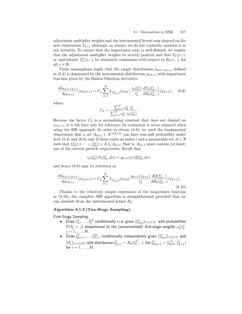
8.1 Alternatives to SISR 257

adjustment multiplier weights and the instrumental kernel may depend on thenew observation Yk+1 although, as always, we do not explicitly mention it inour notation. To ensure that the importance ratio is well-defined, we requirethat the adjustment multiplier weights be strictly positive and that Tk(x, ·),or equivalently T u

k (x, ·), be absolutely continuous with respect to Rk(x, ·), forall x ∈ X.

These assumptions imply that the target distribution φ0:k+1|k+1 definedin (8.4) is dominated by the instrumental distribution ρ0:k+1 with importancefunction given by the Radon-Nikodym derivative

dφ0:k+1|k+1

dρ0:k+1(x0:k+1) = Ck

N∑i=1

1ξi0:k(x0:k)γk(ξik)τ ik

dTk(ξik, ·)dRk(ξik, ·)

(xk+1) , (8.9)

where

Ck =∑Ni=1 ω

ik τ

ik∑N

i=1 ωik γk(ξik)

.

Because the factor Ck is a normalizing constant that does not depend onx0:k+1, it is left here only for reference; its evaluation is never required whenusing the SIR approach. In order to obtain (8.9), we used the fundamentalobservation that a set Ak+1 ∈ X⊗(k+2) can have non-null probability underboth (8.4) and (8.8) only if there exists an index i and a measurable set A ⊆ Xsuch that ξi0× · · · × ξik×A ⊆ Ak+1, that is, Ak+1 must contain (at least)one of the current particle trajectories. Recall that

γk(ξik)Tk(ξik, dx) = gk+1(x)Q(ξik, dx) ,

and hence (8.9) may be rewritten as

dφ0:k+1|k+1

dρ0:k+1(x0:k+1) = Ck

N∑i=1

1ξi0:k(x0:k)gk+1(xk+1)

τ ik

dQ(ξik, ·)dRk(ξik, ·)

(xk+1) ,

(8.10)Thanks to the relatively simple expression of the importance function

in (8.10), the complete SIR algorithm is straightforward provided that wecan simulate from the instrumental kernel Rk.

Algorithm 8.1.3 (Two-Stage Sampling).

First-Stage Sampling:• Draw I1

k , . . . , IMk conditionally i.i.d. given ξi0:k1≤i≤N , with probabilities

P(Iik = j) proportional to the (unnormalized) first-stage weights ωjkτjk ,

j = 1, . . . ,M .• Draw ξ1

k+1, . . . , ξMk+1 conditionally independently given ξl0:k1≤l≤N and

Iik1≤i≤M , with distribution ξik+1 ∼ Rk(ξIik

k , ·). Set ξi0:k+1 = (ξIik

0:k, ξik+1)

for i = 1, . . . ,M .

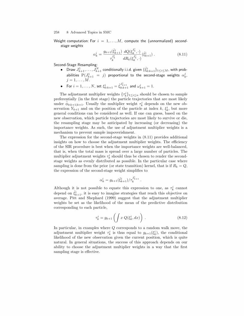
258 8 Advanced Topics in SMC

Weight computation: For i = 1, . . . ,M , compute the (unnormalized) second-stage weights

αik =gk+1(ξik+1)

τIikk

dQ(ξIik

k , ·)

dRk(ξIik

k , ·)(ξik+1) . (8.11)

Second-Stage Resampling:• Draw J1

k+1, . . . , JNk+1 conditionally i.i.d. given ξi0:k+11≤i≤M , with prob-

abilities P(J1k+1 = j) proportional to the second-stage weights αjk,

j = 1, . . . ,M .

• For i = 1, . . . , N , set ξi0:k+1 = ξJik+10:k+1 and ωik+1 = 1.

The adjustment multiplier weights τ ik1≤i≤n should be chosen to samplepreferentially (in the first stage) the particle trajectories that are most likelyunder φ0:k+1|k+1. Usually the multiplier weight τ ik depends on the new ob-servation Yk+1 and on the position of the particle at index k, ξik, but moregeneral conditions can be considered as well. If one can guess, based on thenew observation, which particle trajectories are most likely to survive or die,the resampling stage may be anticipated by increasing (or decreasing) theimportance weights. As such, the use of adjustment multiplier weights is amechanism to prevent sample impoverishment.

The expression for the second-stage weights in (8.11) provides additionalinsights on how to choose the adjustment multiplier weights. The efficiencyof the SIR procedure is best when the importance weights are well-balanced,that is, when the total mass is spread over a large number of particles. Themultiplier adjustment weights τ ik should thus be chosen to render the second-stage weights as evenly distributed as possible. In the particular case wheresampling is done from the prior (or state transition) kernel, that is if Rk = Q,the expression of the second-stage weight simplifies to

αik = gk+1(ξik+1)/τIik+1k .

Although it is not possible to equate this expression to one, as τ ik cannotdepend on ξik+1, it is easy to imagine strategies that reach this objective onaverage. Pitt and Shephard (1999) suggest that the adjustment multiplierweights be set as the likelihood of the mean of the predictive distributioncorresponding to each particle,

τ ik = gk+1

(∫x Q(ξik, dx)

). (8.12)

In particular, in examples where Q corresponds to a random walk move, theadjustment multiplier weight τ ik is thus equal to gk+1(ξik), the conditionallikelihood of the new observation given the current position, which is quitenatural. In general situations, the success of this approach depends on ourability to choose the adjustment multiplier weights in a way that the firstsampling stage is effective.

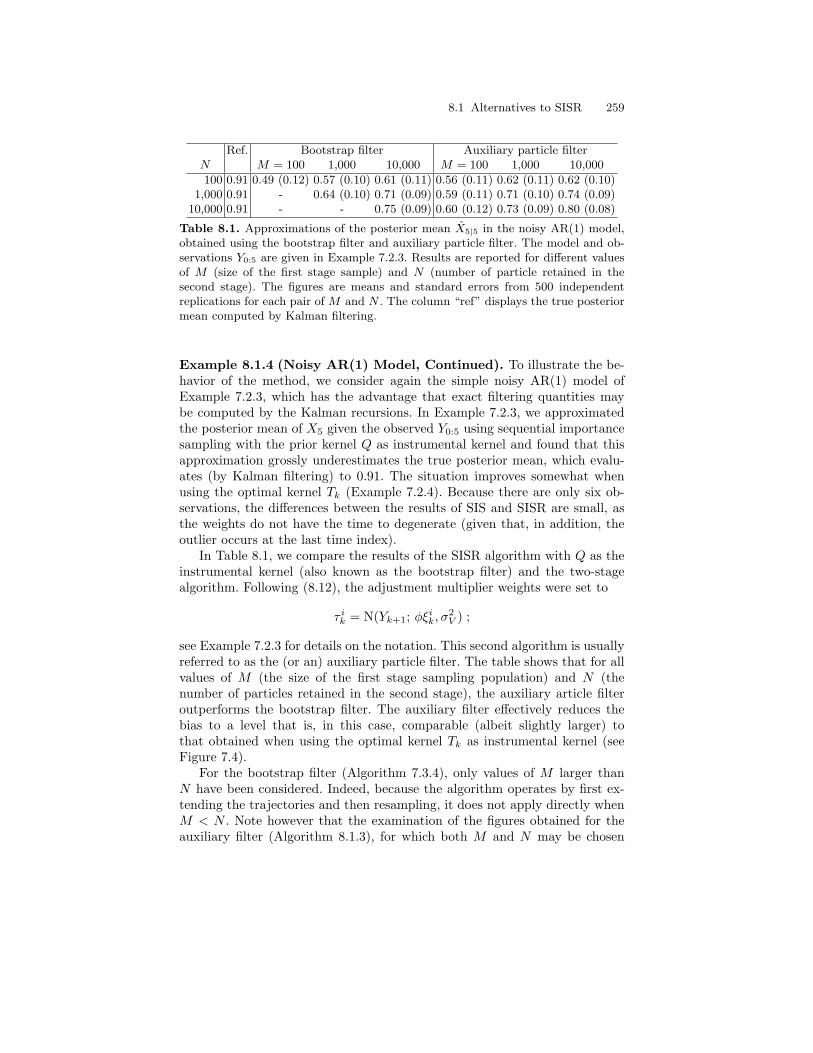
8.1 Alternatives to SISR 259

Ref. Bootstrap filter Auxiliary particle filterN M = 100 1,000 10,000 M = 100 1,000 10,000

100 0.91 0.49 (0.12) 0.57 (0.10) 0.61 (0.11) 0.56 (0.11) 0.62 (0.11) 0.62 (0.10)1,000 0.91 - 0.64 (0.10) 0.71 (0.09) 0.59 (0.11) 0.71 (0.10) 0.74 (0.09)

10,000 0.91 - - 0.75 (0.09) 0.60 (0.12) 0.73 (0.09) 0.80 (0.08)

Table 8.1. Approximations of the posterior mean X5|5 in the noisy AR(1) model,obtained using the bootstrap filter and auxiliary particle filter. The model and ob-servations Y0:5 are given in Example 7.2.3. Results are reported for different valuesof M (size of the first stage sample) and N (number of particle retained in thesecond stage). The figures are means and standard errors from 500 independentreplications for each pair of M and N . The column “ref” displays the true posteriormean computed by Kalman filtering.

Example 8.1.4 (Noisy AR(1) Model, Continued). To illustrate the be-havior of the method, we consider again the simple noisy AR(1) model ofExample 7.2.3, which has the advantage that exact filtering quantities maybe computed by the Kalman recursions. In Example 7.2.3, we approximatedthe posterior mean of X5 given the observed Y0:5 using sequential importancesampling with the prior kernel Q as instrumental kernel and found that thisapproximation grossly underestimates the true posterior mean, which evalu-ates (by Kalman filtering) to 0.91. The situation improves somewhat whenusing the optimal kernel Tk (Example 7.2.4). Because there are only six ob-servations, the differences between the results of SIS and SISR are small, asthe weights do not have the time to degenerate (given that, in addition, theoutlier occurs at the last time index).

In Table 8.1, we compare the results of the SISR algorithm with Q as theinstrumental kernel (also known as the bootstrap filter) and the two-stagealgorithm. Following (8.12), the adjustment multiplier weights were set to

τ ik = N(Yk+1; φξik, σ2V ) ;

see Example 7.2.3 for details on the notation. This second algorithm is usuallyreferred to as the (or an) auxiliary particle filter. The table shows that for allvalues of M (the size of the first stage sampling population) and N (thenumber of particles retained in the second stage), the auxiliary article filteroutperforms the bootstrap filter. The auxiliary filter effectively reduces thebias to a level that is, in this case, comparable (albeit slightly larger) tothat obtained when using the optimal kernel Tk as instrumental kernel (seeFigure 7.4).

For the bootstrap filter (Algorithm 7.3.4), only values of M larger thanN have been considered. Indeed, because the algorithm operates by first ex-tending the trajectories and then resampling, it does not apply directly whenM < N . Note however that the examination of the figures obtained for theauxiliary filter (Algorithm 8.1.3), for which both M and N may be chosen

260 8 Advanced Topics in SMC

freely, suggests that it is more efficient to use M larger than N than the con-verse. The payoff for using M larger than N , compared to the base situationwhere M = N , is also much more significant in the case of the bootstrapfilter—whose baseline performance is worse—than for the auxiliary particlefilter.

8.1.3 Interpretation with Auxiliary Variables

We now discuss another interpretation of Algorithm 8.1.3, which is more inthe spirit of (Pitt and Shephard, 1999). This alternative perspective on Algo-rithm 8.1.3 is based on the observation that although we generally consider ourtarget distributions to be the joint smoothing distribution φ0:k|k, the obtainedalgorithms are directly applicable for approximating the filtering distributionφk simply by dropping the history of the particles (Remark 7.3.5).

In particular, if we now consider that only the current system of particlesξik1≤i≤N , with associated weights ωik1≤i≤N is available, (8.3) should bereplaced by the marginal relation

φk+1(f) def=N∑i=1

ωik γk(ξik)∑Nj=1 ω

jk γk(ξjk)

∫f(x) Tk(ξik, dx) , f ∈ Fb (X) , (8.13)

which thus defines our target distribution for updating the system of particles.For the same reason as above, it makes sense to select a proposal distri-

bution (this time on X) closely related to (8.13). Indeed, we consider the Ncomponent mixture

ρk+1(f) =N∑i=1

ωikτik∑N

j=1 ωjkτjk

∫f(x)Rk(ξik, dx) . (8.14)

Proceeding as in (8.9)–(8.10), the Radon-Nikodym derivative is now givenby

dφν,k+1

dρk+1(x) = Ck

d∑N

i=1 ωik Tk(ξik, ·)

d∑N

i=1 ωikτjk Rk(ξik, ·)

(x) . (8.15)

Compared to (8.10), this marginal importance ratio would be costly to eval-uate as such, as both its numerator and its denominator involve summingover N terms. This difficulty can be overcome by data augmentation, intro-ducing an auxiliary variable that corresponds to the mixture component thatis selected when drawing the new particle position. Consider the followingdistribution φaux

k+1 on the product space 1, . . . , N × X:

φauxk+1(i ×A) =

ωik∫Agk+1(x)Q(ξik, dx)∑Nj=1 ω

jkγk(ξjk)

, A ∈ X , i = 1, . . . , N . (8.16)

8.1 Alternatives to SISR 261

Because

φauxk+1(1, . . . , N ×A) =

N∑i=1

φauxk+1(i ×A) = φk+1(A) , A ∈ X ,

φk+1 is the marginal distribution of φauxk+1 and we may sample from φk+1 by

sampling from φauxk+1 and discarding the auxiliary index. To sample from φaux

k+1

using the SIR method, we can then use the following instrumental distributionon the product space 1, . . . , N × X:

ρauxk+1(i ×A) =

ωik τik∑N

j=1 ωjk τ

jk

Rk(ξik, A) , A ∈ X . (8.17)

This distribution may be interpreted as the joint distribution of the selectionindex Iik and the proposed new particle position ξik+1 in Algorithm 8.1.3. Thistime, the importance function is very simple and similar to (8.10),

dφauxk+1

dρauxk+1

(i, x) = Ckgk+1(x)τ ik

dQ(ξik, ·)dRk(ξik, ·)

(x) , i = 1, . . . , N, x ∈ X , (8.18)

Hence Algorithm 8.1.3 may also be understood in terms of auxiliary sampling.

8.1.4 Auxiliary Accept-Reject Sampling

Rather than using the SIR method, simulating from (8.17) and using the im-portance ratio defined in (8.18), we may consider other methods for simulatingdirectly from (8.16). An option, already discussed in the context of sequen-tial importance sampling in Section 7.2.2, consists in using the accept-rejectmethod (defined in Section 6.2.1).

The accept-reject method may be used to generate a truly i.i.d. samplefrom the target distribution. The price to pay compared to the SIR algorithmis a typically higher computational cost, especially when the acceptance prob-ability is low. In addition, the number of simulations needed is itself randomand the computation time cannot be predicted beforehand, especially whenthere are unknown normalizing constants (Remark 6.2.4). The method hasnonetheless been studied for sequential simulation by several authors includ-ing Tanizaki (1996), Tanizaki and Mariano (1998), and Hurzeler and Kunsch(1998) (see also Pitt and Shephard, 1999, and Liu and Chen, 1998).

In auxiliary accept-reject the idea is to find an instrumental distributionρauxk+1 that dominates the target φaux

k+1 and is such that the Radon-Nikodymderivative dφaux

k+1/dρauxk+1 is bounded. Indeed, proposals of the form given

in (8.8) still constitute an appropriate choice granted that we strengthen some-what the assumptions that were needed for applying the SIR method.

Assumption 8.1.5. For any k ≥ 0 and x ∈ X,

supx′∈X

gk+1(x′)dQ(x, ·)dRk(x, ·)

(x′) <∞ . (8.19)

262 8 Advanced Topics in SMC

Because the index i runs over a finite set 1, . . . , N, we may define

Mk = max1≤i≤N

Aikτ ik

, where Aik ≥ supx∈X

gk+1(x)dQ(ξik, ·)dRk(ξik, ·)

(x) . (8.20)

With these definitions, the Radon-Nikodym derivative dφauxk+1/dρ

auxk+1 given

by (8.18) is bounded by

dφauxk+1

dρauxk+1

(i, x) ≤Mk

∑Ni=1 ω

ik τ

ik∑N

i=1 ωik γk(ξik)

, (8.21)

and hence the use of the accept-reject algorithm is valid. The complete algo-rithm proceeds as follows.

Algorithm 8.1.6 (Auxiliary Accept-Reject). For i = 1, . . . , N ,

Repeat:• Draw an index Iik ∈ 1, . . . , N with probabilities proportional to the

first-stage weights ω1kτ

1k , . . . , ω

Nk τ

Nk .

• Conditionally on Iik, draw a proposal ξik+1 from the instrumental transition

kernel Rk(ξIik

k , ·) and U i from a uniform distribution on [0, 1].Until:

U i ≤ 1Mk

gk+1(ξik+1)

τIikk

dQ(ξIik

k , ·)

dRk(ξIik

k , ·)(ξik+1) .

Update: Set ξik+1 = ξik+1.

When done, reset all weights ωik+11≤i≤N to a (common) constant value.

Because the joint distribution of the accepted pairs is φauxk+1, as defined

by (8.16), the marginal distribution of the accepted draws (forgetting aboutthe index) is (8.13) as required. One should typically try to increase the ac-ceptance rate by proper choices of the adjustment multiplier weights τ ik and,whenever possible, by also choosing the instrumental kernel Rk in an appro-priate fashion. The user should also determine the upper bounds Aik in (8.20)as tightly as possible. The following lemma, due to Kunsch (2003), gives someindications on how the multiplier weights should be chosen to maximize theacceptance ratio.

Lemma 8.1.7. For a given choice of instrumental kernels Rk and upperbounds Aik, the average acceptance probability is maximal when the incremen-tal adjustment weights τ ik are proportional to Aik for i = 1, . . . , N .

Proof. Recall from Remark 6.2.4 that because of the presence of unknown nor-malization constants, the acceptance probability of the accept-reject methodis not 1/Mk but rather the inverse of the upper bound on the importancefunction, that is, the right-hand side of (8.21). Because

8.1 Alternatives to SISR 263

∑Ni=1 ω

ik τ

ik∑N

i=1 ωik γk(ξik)

Mk ≥

∑Ni=1 ω

ik τ

ikAikτ ik∑N

i=1 ωik γk(ξik)

=∑Ni=1 ω

ik A

ik∑N

i=1 ωik γk(ξik)

,

the acceptance probability is bounded by∑Ni=1 ω

ik γk(ξik)∑N

i=1 ωik A

ik

. (8.22)

The bound is attained when Aik/τik = Mk for all i. ut

Tanizaki and Mariano (1998) and Hurzeler and Kunsch (1998) both con-sider the particular choice Rk = Q. Lemma 8.1.7 shows that the optimaladjustment multiplier weights are then constant, τ ik = 1 for all i. This issomewhat surprising in light of the discussion in Section 8.1.2, as one couldconjecture heuristically that it is more appropriate to favor particles that agreewith the next observations. Lemma 8.1.7 however shows that the only meansto improve the acceptance rate is, whenever possible, to properly optimize theinstrumental kernel.

8.1.5 Markov Chain Monte Carlo Auxiliary Sampling

Rather than using the accept-reject algorithm to sample exactly from (8.16),Berzuini et al. (1997) suggest that a few iterations of a Markov chain MonteCarlo sampler with target distribution (8.16) be used. The algorithm proposedby Berzuini et al. (1997) is based on the independent Metropolis-Hastingssampler discussed in Section 6.2.3.1. Once again, we use a distribution ρaux

k+1

of the form defined in (8.8) as the proposal, but this time the chain movesfrom (i, x) to (i′, x′) with a probability given by A[(i, x), (i′, x′)] ∧ 1 where

A [(i, x), (i′, x′)] =[gk+1(x′)τ i′k

dQ(ξik, ·)dRk(ξik, ·)

(x′)] [

gk+1(x)τ ik

dQ(ξik, ·)dRk(ξik, ·)

(x)]−1

.

(8.23)In case of rejection, the chain stays in (i, x). This update step is then repeatedindependently N times.

Algorithm 8.1.8 (Auxiliary MCMC). For i = 1, . . . , N ,

Initialization: Draw an index Ii,1k ∈ 1, . . . , N with probabilities proportional

to the first-stage weights ω1kτ

1k , . . . , ω

Nk τ

Nk , and ξi,1k+1 from the instrumental

transition kernel Rk(ξIi,1k

k , ·). Set ξik+1 = ξi,1k+1 and Iik = Ii,1k .

For j = 2 to Jmax: Draw an index Ii,jk ∈ 1, . . . , N with probabilities propor-

tional to the first-stage weights ω1kτ

1k , . . . , ω

Nk τ

Nk , draw ξi,jk+1 from the instru-

mental transition kernel Rk(ξIi,jk

k , ·) and a U([0, 1]) variable U j . If

U j ≤ A[(Iik, ξik+1), (Ii,jk , ξi,jk+1)] ,

set ξik+1 = ξi,jk+1 and Iik = Ii,jk .

264 8 Advanced Topics in SMC

When done, all weights ωik+11≤i≤N are reset to a constant value.

In the above algorithm, ρauxk+1 is used both as proposal distribution for

the independent Metropolis-Hastings sampler and for generating the initialvalues Ii,1k and ξi,1k+1. Compared to the accept-reject approach of the previoussection, Algorithm 8.1.8 is appealing, as it is associated with a deterministiccomputation time that scales like the product of N and Jmax. On the otherhand, the method can only be useful if Jmax is “small” which in turn islegitimate only if the independent Metropolis-Hastings chain is fast mixing.As discussed in Section 6.2.3.1, the mixing of each individual chain is governedby the behavior of the quantity

M ik = sup

x∈X

gk+1(x)τ ik

dQ(ξik, ·)dRk(ξik, ·)

(x) ,

and the chain is uniformly (geometrically) ergodic, at rate (1 − 1/M ik), only

if M ik is finite. Not surprisingly, this approach thus shares many common fea-

tures and properties with the accept-reject algorithm discussed in the previoussection. It is of course possible to combine both methods (Tanizaki, 2003) orto resort to other type of MCMC samplers. We refer to Berzuini and Gilks(2001) for a full discussion of this approach together with some exampleswhere it is particularly useful.

8.2 Sequential Monte Carlo in Hierarchical HMMs

In Section 4.2, we examined a general class of HMMs, referred to as hierarchi-cal HMMs, for which the state can be partitioned into two components, oneof which can be analytically integrated out—or marginalized—conditionallyon the other component. When marginalization is feasible, one may derivecomputationally efficient sampling procedures that focus their full attentionon a state space whose dimension is smaller—and in most applications, muchsmaller—than the original one. As a result, when marginalization is feasible,it usually significantly improves the performance of particle filtering, allowingin particular a drastic reduction of the number of particles needed to achieve agiven level of accuracy of the estimates (Akashi and Kumamoto, 1977; Liu andChen, 1998; MacEachern et al., 1999; Doucet et al., 2000a,b). One should how-ever keep in mind that marginalization requires the use of rather sophisticatedalgorithms, and that the computations necessary to update each marginal par-ticle can be much more demanding than for an unstructured particle that livesin the complete state space.

Marginalizing out some of the variables is an example of a classical tech-nique in computational statistics referred to as the Rao-Blackwellization, be-cause it is related to the Rao-Blackwell risk reduction principle in statistics.Rao-Blackwellization is an important ingredient of simulation-based methodsthat we already met in the context of MCMC methods in Chapter 6.

8.2 Sequential Monte Carlo in Hierarchical HMMs 265

In the hierarchical hidden Markov model introduced in Section 1.3.4, thestate variable Xk can be decomposed in two parts (Ck,Wk), where Ck is calledthe indicator variable or the regime and Wk is the partial state, which can bemarginalized out conditionally on the regime. We will focus on the special casewhere the indicator variables are discrete and finite. Although it is possible touse the marginalization principle in a more general setting (see, e.g., Doucetet al., 2001b, or Andrieu et al., 2003), the case of discrete indicator variablesremains the most important in practical applications.

8.2.1 Sequential Importance Sampling and Global Sampling

Assume that the indicator variables take their values in the finite set C =1, . . . , r. We consider here, as previously, that the goal is to simulate fromthe sequence of joint probability measures ψ0:k|kk≥0 of C0:k given Y0:k. Forthe moment, the details of the structure of ψ0:k|k do not matter and we simplyassume that there exists an (unnormalized) transition kernel T u

k : Ck+1×C→R+ such that

ψ0:k+1|k+1(c0:k+1) = ψ0:k|k(c0:k)T uk (ck, ck+1) . (8.24)

Note that as usual for probabilities on discrete spaces, we use the notationψ0:k|k(c0:k) rather than ψ0:k|k(c0:k). This definition should be compared to(7.8). Indeed, T u

k is an unnormalized kernel similar to that which appears in(7.8), although it does not depend—as a function of c0:k—on ck only. Thismodification is due to the fact that the structure of the joint smoothing distri-bution in hierarchical HMMs, when marginalizing with respect to the interme-diate component Wk, is more complex than in the models that we have metso far in this chapter (see Section 4.2.3). Once again, these considerations arenot important for the moment, and the reader should consider (8.24) as thedefinition of a (generic) sequence of probability distributions over increasingspaces.

8.2.1.1 Sequential Importance Sampling

In the sequential importance sampling framework, the target distributionat time k is approximated by independent path particles denoted, as pre-viously, by ξ1

0:k, . . . , ξN0:k, associated with non-negative (normalized) weights(

ω1k, . . . , ω

Nk

)such that

ψ0:k|k(c0:k) =N∑i=1

ωik1ξi0:k(c0:k) . (8.25)

These particles and weights are updated sequentially by drawing from aninstrumental distribution over sequences in CN defined by an initial probability

266 8 Advanced Topics in SMC

distribution ρ0:0 on C and a family of transition kernels Rk : Ck+1×C→ R+,for k ≥ 0, such that

ρ0:k+1(c0:k+1) = ρ0:k(c0:k)Rk(c0:k, ck+1) , (8.26)

where ρ0:k denotes the joint distribution of ξ10:k. It is assumed that for each k,

the instrumental kernel Rk dominates the transition T uk in the sense that

for any c0:k and any c = 1, . . . , r, the condition T uk (c0:k, c) > 0 implies

Rk(c0:k, c) > 0. In words, all transitions that are permitted (have positiveprobability) under the model are permitted also under the instrumental ker-nel. In the sequential importance sampling procedure, one draws exactly onesuccessor for each path particle ξi0:k, i = 1, . . . , N . More precisely, an N -upletI1k+1, . . . , I

Nk+1 is drawn conditionally independently given the past and with

probabilities proportional to the weights

Rk(ξi0:k, 1), . . . , Rk(ξi0:k, r) .

The particle system is then updated according to ξi0:k+1 = (ξi0:k, Iik+1). If

ξ10 , . . . , ξ

N0 are drawn independently from a probability distribution ρ0:0, the

particle system ξ10:k, . . . , ξ

N0:k consists of N independent draws from the instru-

mental distribution ρ0:k. As in (7.13), the associated (unnormalized) impor-tance weights can be written as a product of incremental weights

ωik+1 = ωikT uk (ξi0:k, I

ik+1)

Rk(ξi0:k, Iik+1)

. (8.27)

The instrumental transition kernel that minimizes the variance of the im-portance weights conditionally on the history of the particle system will bedenoted by Tk and is given by the analog of (7.15):

Tk(c0:k, c) =T uk (c0:k, c)

T uk (c0:k,C)

, c0:k ∈ Ck+1, c ∈ C . (8.28)

This kernel is referred to as the optimal instrumental kernel. The importanceweights (8.27) associated with this kernel are updated according to

ωik+1 = ωikTuk (ξi0:k,C) . (8.29)

As before, these incremental importance weights do not depend on the de-scendant of the particle. The SIS algorithm using the optimal importancekernel is equivalent to the random sampling algorithm of Akashi and Ku-mamoto (1977). In this scheme, resampling is stochastic with precisely onedescendant of each particle at time k being kept. For each particle, a de-scendant is chosen with probabilities proportional to the descendant’s weightsT uk (ξi0:k, 1), . . . , T u

k (ξi0:k, r). The weight of the chosen particle is set to the prod-uct of its parent’s weight and the sum

∑rc=1 T

uk (ξi0:k, c).

8.2 Sequential Monte Carlo in Hierarchical HMMs 267

8.2.1.2 Global Sampling

As in the previous chapter, the particle system produced by sequential im-portance sampling degenerates, and the way to fight this degeneracy is re-sampling. Because the state space is finite however, we now can probe thewhole state space because each particle has a finite number (r) of possible de-scendants. The sampling and resampling steps may then be combined into asingle random draw. Recall that a natural estimator of the target distributionψ0:k|k at time k is the empirical distribution of the particles defined in (8.25).Equation (8.24) suggests to estimate the probability distribution Πk+1 by

ψ0:k+1|k+1(c0:k+1) =

∑Ni=1 ω

ikδξi0:k

(c0:k)T uk (ξi0:k, ck+1)∑N

i=1 ωikT

uk (ξi0:k,C)

. (8.30)

This equation corresponds to (8.4) in the current discrete setting. The sup-port of this distribution is included in the set of all the possible descendantsof the current system of particles. Each particle has at most r possible de-scendants and thus the support of this distribution has at most N × r points.A straightforward solution (see for instance Fearnhead and Clifford, 2003) tosample from this distribution is as follows.

Algorithm 8.2.1 (Global Sampling).

Weighting: For i = 1, . . . , N and j = 1, . . . , r, compute the (normalized) weights

ωi,jk+1 =ωikT

uk (ξi0:k, j)∑N

l=1

∑rc=1 ω

lkT

uk (ξi0:k, c)

. (8.31)

Sampling : Conditionally independently from the particle system history, draw Nidentically distributed pairs (Iik, J

ik+1) ∈ 1, . . . , N × 1, . . . , r, for i =

1, . . . N , such that P[(I1k , J

1k+1) = (i, j) | Gk] = ωi,jk+1, where Gk is the σ-field

generated by the history of the particle system up to time k.

Update: Set ξi0:k+1 = (ξIik

0:k, Jik+1) and ωik+1 = 1/N for i = 1, . . . , N .

Remark 8.2.2. There are several closely related algorithms that have ap-peared in the literature, in particular the detection estimation algorithm ofTugnait (1984). In this algorithm, the resampling stage is deterministic, withthe N particles having largest weights being kept. The application of suchideas has been especially investigated in digital communication applicationsand is discussed, for instance, by Punskaya et al. (2002) and Bertozzi et al.(2003).

8.2.2 Optimal Sampling

As stressed in Section 7.4.2, there are other options to draw the reallocationvariables such as residual, stratified, or systematic resampling. Although these

268 8 Advanced Topics in SMC

can certainly be useful in this context, the discrete nature of the state space hasan unexpected consequence that is not addressed properly by the resamplingtechniques discussed so far. For problems in which the state space is continu-ous, having multiple copies of particles is not detrimental. After resampling,each copy of a given duplicated particle will evolve independently from theothers. Therefore, a particle with a large importance weight that is replicatedmany times in the resampling stage may, in the future, have a large number ofdistinct descendants. When the state space is finite however, each particle canprobe all its possible descendants (ξi0:k, j) such that T u

k (ξi0:k, j) > 0. Hence,if the resampling procedure replicates a particle at time k, the replications ofthis particle will probe exactly the same configurations in the future. Havingmultiple copies of the same path particle in finite state space models is thusparticularly wasteful.

A possible solution to this problem has been suggested by Fearnhead andClifford (2003) under the name optimal sampling. Instead of drawing realloca-tion variables (Iik, J ik+1)1≤i≤N , we sample non-negative importance weightsW i,j

k+1 satisfying the constraints

N∑i=1

r∑j=1

1W i,jk+1>0 ≤ N (8.32)

E[W i,jk+1 | Gk] = ωi,jk+1, i = 1, . . . , N, j = 1, . . . , r, (8.33)

where the weights ωi,jk+1 are defined in (8.31). The first constraint is thatthere are at most N particles with non-zero weights. The second constraint isthat the importance weights be unbiased—in the terminology of Liu and Chen(1998) or Liu et al. (2001), the new sample is the said to be properly weighted.A word of caution is needed here: despite the fact that the unbiasednesscondition is very sensible in the context of resampling, it does not, in itself,guarantee a proper behavior of the algorithm (more on this will be said inChapter 9). Conversely, exact unbiasedness is not absolutely necessary, and itis perfectly possible to consider algorithms that exhibit a low, and controllable,bias. The problem reduces to that of approximating a probability distributionhaving M = N × r points of support by a random probability distributionhaving at most N points of support. Resampling is equivalent to assigninga new, random weight to each of the M = N × r particles. If the weight iszero the particle is removed, whereas if the weight is non-zero the particle iskept; the non-zero random variables W i,j

k+1 represent the new weights of thedescendants of the particle system.

In a more general perspective, the problem can be formulated as follows.Let ω be a discrete probability distribution with M points of support

ω = (ω1, . . . , ωM ), ωi ≥ 0,M∑i=1

ωi = 1 . (8.34)

8.2 Sequential Monte Carlo in Hierarchical HMMs 269

We want to find a random probability distribution W = (W1, . . . ,WM ) on1, . . . ,M with at most N ≤M points of support,

Wi ≥ 0 ,M∑i=1

Wi = 1 ,M∑i=1

1Wi>0 ≤ N , (8.35)

satisfyingE[Wi] = ωi, i = 1, . . . ,M . (8.36)

There are of course a number of different ways to achieve (8.35) and(8.36). In particular, all the resampling methods discussed in Section 7.4.2(as well as multinomial resampling) draw integer counts Ni, which are suchthat Wi = Ni/N satisfy the above requirements, with equality for the lastcondition in (8.35). The “optimal” solution is the one that guarantees thatthe random distribution W is close, in some suitable sense, to the target dis-tribution ω. We follow the suggestion of Fearnhead and Clifford (2003) anduse the average L2 distance. The problem then becomes equivalent to findinga random probability distribution W = (W1, . . . ,WM ) that minimizes

M∑i=1

E(Wi − ωi)2 (8.37)

subject to (8.35) and (8.36). To compute the solution we rely on two lemmas.

Lemma 8.2.3. Let ω ≥ 0 and p ∈ (0, 1]. If W is a non-negative randomvariable satisfying

E[W ] = ω and P(W > 0) = p , (8.38)

thenE(W − ω)2 ≥ 1− p

pω2 . (8.39)

The lower bound is attained by any random variable W such that W equalsω/p on the subset of the sample space where W > 0.

Proof. By decomposing the sample space into W > 0 and W = 0, weobtain

ω = E[W ] = E[W |W > 0] P(W > 0) = E[W |W > 0]p , (8.40)

and by a similar decomposition,

E(W − ω)2 = E[(W − ω)2 |W > 0]p+ ω2(1− p) . (8.41)

A bias-variance decomposition of E[(W − ω)2 |W > 0] then gives

270 8 Advanced Topics in SMC

E[(W − ω)2 |W > 0]

= E[(W − E[W |W > 0])2 |W > 0] + (E[W |W > 0]− ω)2

= E[(W − E[W |W > 0])2 |W > 0] + ω2 (1− p)2

p2,

where we used (8.40) to obtain the second equality. The right-hand side of thisdisplay is bounded from below by ω2(1 − p)2/p2, and inserting this into theright-hand side of (8.41) we obtain (8.39). Using the last display once again, wealso see that the bound is attained if and only if W equals E[W |W > 0] = ω/pon the set where W > 0. ut

Lemma 8.2.4. Let N < M be integers and let β1, . . . , βM be non-negativenumbers. Consider the problem

minimizeM∑j=1

βjpj

subject toM∑j=1

pj ≤ N ,

0 ≤ pj ≤ 1, j = 1, . . . ,M .

This problem has a unique solution given by

pj = µ√βj ∧ 1, j = 1, . . . ,M , (8.42)

where the constant µ is the unique solution of the equation

M∑i=1

µ√βj ∧ 1 = N . (8.43)

Proof. Denote by λ and λi the Lagrange multipliers associated respectivelywith the inequality constraints

∑Mi=1 pi ≤ N and pi ≤ 1, i = 1, . . . ,M . The

Karush-Kuhn-Tucker conditions (see Boyd and Vandenberghe, 2004) for theprimal p1, . . . , pM and dual λ, λ1, . . . , λM optimal points are given by

M∑i=1

pi ≤ N, pi ≤ 1, i = 1, . . . ,M , (8.44)

λ ≥ 0, λi ≥ 0, i = 1, . . . ,M , (8.45)

λ

(M∑i=1

pi −N

)= 0, λi(pi − 1) = 0, i = 1, . . . ,M , (8.46)

− βip2i

+ λ+ λi = 0, i = 1, . . . ,M . (8.47)

8.2 Sequential Monte Carlo in Hierarchical HMMs 271

The complementary slackness condition (8.46) implies that for all indices isuch that pi < 1, the corresponding multiplier λi is zero. Hence, using (8.47),

pi =

√βiλ∧ 1, i = 1, . . . ,M . (8.48)

From this we see that if λ = 0, then pi = 1 for all i and (8.44) cannot be satis-fied. Thus λ > 0, and the complementary slackness condition (8.46) thereforeimplies that

∑Mi=1 pi = N . Plugging (8.48) into this equation determines the

multiplier λ by solving for λ in the equation∑M

1

√βi/λ ∧ 1 = N . ut

By combining these two lemmas, we readily obtain a characterization ofthe random distribution achieving the minimal average divergence (8.37) sub-ject to the support constraint

∑Mi=1 P(Wi > 0) ≤ N and the unbiasedness

constraint (8.36).

Proposition 8.2.5. Let W = (W1, . . . ,WM ) be a random vector with non-negative entries. This vector is a solution to the problem

minimizeM∑i=1

E(Wi − ωi)2

subject toM∑i=1

P(Wi > 0) ≤ N ,

E[Wi] = ωi, i = 1, . . . ,M ,

if and only if for any i = 1, . . . ,M ,

Wi =

ωi/pi with probability pi

def= µωi ∧ 1 ,0 otherwise ,

(8.49)

where µ is the unique solution of the equation

M∑i=1

µωi ∧ 1 = N . (8.50)

Proof. Put pi = P(Wi > 0). By Lemma 8.2.3,

M∑i=1

E(Wi − ωi)2 ≥M∑i=1

ω2i

pi−

M∑i=1

ω2i . (8.51)

The proof follows from Lemma 8.2.4. ut

Remark 8.2.6. Note that if µωi ≥ 1, then pi = 1 and ωi/pi = ωi. Thus (8.49)implies that weights exceeding a given threshold (depending on the weights

272 8 Advanced Topics in SMC

themselves) are left unchanged. For a particle i whose weight falls below thisthreshold, the algorithm proceeds as follows. With probability 1− pi > 0, theweight is set to zero; otherwise it is set (and thus increased) to ωi/pi = 1/µin order to satisfy the unbiasedness condition. The algorithm is related tothe procedure proposed in Liu et al. (2001) under the name partial rejectioncontrol.

The above proposition describes the marginal distribution of the Wi thatsolves (8.37). The following result proposes a simple way to draw randomweights (W1, . . . ,WM ) that satisfy (8.49) with

∑Mi=1 1Wi>0 = N .

Proposition 8.2.7. Let µ be the solution of (8.50),

Sdef= i ∈ 1, . . . ,M : µωi ≥ 1 (8.52)

and pi = µωi ∧ 1. Let U be a uniform random variable on (0, 1) and set

Ni =⌊∑

j 6∈S, j≤i pj + U⌋−⌊∑

j 6∈S, j<i pj + U⌋, i = 1, . . . ,M ,

with b·c being the integer part. Define the random vector W = (W1, . . . ,WM )by

Wi =

ωi if i ∈ S ,

1/µ if i 6∈ S and Ni > 0 ,0 if i 6∈ S and Ni = 0 .

(8.53)

Then W satisfies (8.49) and

M∑i=1

1Wi>0 = N , (8.54)

M∑i=1

Wi = 1 . (8.55)

Proof. We first show that P(Wi > 0) = pi. For i ∈ S this is immediate, withpi = 1. Thus pick i 6∈ S. Then

Ni ≤ supx≥0

(bx+ pic − bxc) ≤ 1 .

Therefore Ni = 1Wi>0, which implies P(Wi > 0) = P(Ni > 0) = E[Ni]. Itis straightforward to check that the expectation of Ni is the difference of thetwo sums involved in its definition, whence E[Ni] = pi. Thus P(Wi > 0) = pi,showing that (8.49) is satisfied.

Next observe that∑M

1 1Wi>0 = |S| +∑i 6∈SNi. The sum of Ni over all

i 6∈ S is a telescoping one, whence

8.2 Sequential Monte Carlo in Hierarchical HMMs 273

M∑i=1

1Wi>0 = |S|+⌊∑

i 6∈S pi + U⌋− bUc

= |S|+ bN − |S|+ Uc − bUc = |S| − (N − |S|) = N ,

where we used∑i 6∈S pi =

∑M1 pi−

∑i∈S pi = N − |S| for the second equality.

Thus we have (8.54).Finally,

M∑i=1

Wi =∑i∈S

ωi +∑i∈S

Ni/µ .

From the above, we know that the second sum on the right-hand side equals(N − |S|)/c. Because, by definition, ωi/pi = 1/µ for i 6∈ S, the first sum is∑

i∈S

ωi = 1−∑i6∈S

ωi = 1− µ−1∑i 6∈S

pi = 1− N − |S|µ

.

We conclude that∑M

1 Wi = 1, that is, (8.55) holds. utBack to our original problem, Proposition 8.2.7 suggests the following sam-

pling algorithm.

Algorithm 8.2.8 (Optimal Sampling).

Weighting : For i = 1, . . . , N and j = 1, . . . , r, compute the weights

ωi,jk+1 =ωikT

uk (ξi0:k, j)∑N

l=1

∑rc=1 ω

lkT

uk (ξi0:k, c)

. (8.56)

Sampling:• Determine the solution µk+1 of the equation

N∑i=1

r∑j=1

µk+1ωi,jk+1 ∧ 1 = N .

• Draw U ∼ U([0, 1]) and set S = 0.• For i = 1, . . . , N and j = 1, . . . , r,

– If µk+1ωi,jk+1 ≥ 1, then set W i,j

k+1 = ωi,jk+1.

– If µk+1ωi,jk+1 < 1, then set

W i,jk+1 =

µ−1k+1 if bµk+1(S + ωi,jk+1) + Uc − bµk+1S + Uc > 0 ,0 otherwise ,

and set S = S + ωi,jk+1.

Update: For i = 1, . . . , N and j = 1, . . . , r, if W i,jk+1 > 0 set

ξI(i,j)0:k+1 = (ξi0:k, j) ,

ωI(i,j)k+1 = W i,j

k+1 , where I(i, j) =i∑l=1

j−1∑c=1

1W l,ck+1>0 .

274 8 Advanced Topics in SMC

8.2.3 Application to CGLSSMs

In this section, we consider conditionally Gaussian linear state-space models(CGLSSMs), introduced in Section 1.3.4 and formally defined in Section 2.2.3.Recall that a CGLSSM is such that

Wk+1 = A(Ck+1)Wk +R(Ck+1)Uk , (8.57)Yk = B(Ck)Wk + S(Ck)Vk ,

where

• Ckk≥0 is a Markov chain on the finite set C = 1, . . . , r, with transitionkernel QC and initial distribution νC ;

• the state noise Ukk≥0 and measurement noise Vkk≥0 are independentmultivariate Gaussian white noises with zero mean and identity covariancematrices;

• the initial partial state W0 is assumed to be independently N(µν , Σν)distributed;

• A, B, R, and S are known matrix-valued functions of appropriate dimen-sions.

Efficient recursive procedures, presented in Section 5.2.6, are available tocompute the filtered or predicted estimate of the partial state and the as-sociated error covariance matrix conditionally on the indicator variables andobservations. By embedding these algorithms in the sequential importancesampling resampling framework, it is possible to derive computationally ef-ficient sampling procedures that operate in the space of indicator variables(Doucet et al., 2000a; Chen and Liu, 2000). Recall in particular that the ker-nel T u

k in (8.24) has an expression given by (4.11), which we repeat below.

T uk (c0:k, ck+1) =

(Lk+1

Lk

)−1

QC(ck, ck+1)×∫W

gk+1(ck+1, wk+1)ϕk+1|k(c0:k+1, wk+1) dwk+1 , (8.58)

for c0:k+1 ∈ Ck+2, where

• Lk is the likelihood of the observations up to time k;• gk+1(ck+1, wk+1) = g [(ck+1, wk+1), Yk+1] is the value of the transition

density function of the observation Yk+1 given the state and indicatorvariables, that is,

gk+1(ck+1, wk+1) = N(Yk+1;B(ck+1)wk+1, S(ck+1)St(ck+1)) , (8.59)

with N(·;µ,Σ) being the density of the Gaussian multivariate distributionwith mean µ and covariance matrix Σ;

8.2 Sequential Monte Carlo in Hierarchical HMMs 275

• ϕk+1|k(c0:k+1, wk+1) is the density of the predictive distribution of thepartial state Wk+1 given the observations up to time k and the indicatorvariables up to time k + 1:

ϕk+1|k(c0:k+1, wk+1) = N(wk+1; Wk+1|k(c0:k+1), Σk+1|k(c0:k+1)

),

(8.60)where Wk+1|k(c0:k+1) and Σk+1|k(c0:k+1) denote respectively the condi-tional mean and error covariance matrix of the prediction of the par-tial state Wk+1 in terms of the observations Y0:k and indicator variablesC0:k+1 = c0:k+1—these quantities can be computed recursively using theKalman one-step prediction/correction formula (see Section 5.2.3).

As discussed in Section 4.2.3, the distribution of the partial stateWn condi-tional on the observations up to time n is a mixture of rn+1 components—here,Gaussian components—with weights given by ψ0:n|n. In the particle approx-imation, each particle ξi0:n relates to a single term in this mixture. Particleapproximation of the filtering distribution ϕn|n of the partial state Wn thusconsists in recursively choosing N components out of a growing mixture ofrn+1 components and adjusting accordingly the weights of the componentswhich are kept; hence the name mixture Kalman filter proposed by Chen andLiu (2000) to describe this approach.

Algorithm 8.2.9 (Mixture Kalman Filter).

Initialization: For i = 1, . . . , r, compute

ξi0 = i ,

ωi0 = N(Y0;B(i)µν , B(i)ΣνBt(i) + S(i)St(i)) νC(c0) ,

K0(ξi0) = Bt(i)Σν[B(i)ΣνBt(i) + S(i)St(i)

]−1,

W0|0(ξi0) = µν +K0(ξi0) [Y0 −B(i)µν ] ,

Σ0|0(ξi0) = Σν −K0(ξi0)B(i)Σν .

Recursion:Computation of weights: For i = 1, . . . , N and j = 1, . . . , r, compute

Wk+1|k(ξi0:k, j) = A(j)Wk|k(ξi0:k) ,

Σk+1|k(ξi0:k, j) = A(j)Σk|k(ξi0:k)At(j) +R(j)Rt(j) ,

Yk+1|k(ξi0:k, j) = B(j)Wk+1|k(ξi0:k, j) ,

Γk+1(ξi0:k, j) = B(j)Σk+1|k(ξi0:k, j)Bt(j) + S(j)St(j) ,

ωi,jk+1 = ωik N(Yk+1 ; Yk+1|k(ξi0:k, j), Γk+1(ξi0:k, j))QC(ξik, j) .

(First Option) Importance Sampling Step: For i = 1, . . . , N , draw J ik+1 in

1, . . . , r with probabilities proportional to ωi,1k , . . . , ωi,rk , conditionallyindependently of the particle history, and set

276 8 Advanced Topics in SMC

ξi0:k+1 = (ξi0:k, Jik+1) ,

ωik+1 =r∑j=1

ωi,jk+1

/N∑i=1

r∑j=1

ωi,jk+1 ,

Kk+1(ξi0:k+1) = Σk+1|k(ξi0:k, Jik+1)Bt(J ik+1)Γ−1

k+1(ξi0:k+1, Jik+1) ,

Wk+1|k+1(ξi0:k+1) = Wk+1|k(ξi0:k, Jik+1)

+Kk+1(ξi0:k+1)[Yk+1 − Yk+1|k(ξi0:k, J

ik+1)

],

Σk+1|k+1(ξi0:k+1) =[I −Kk+1(ξi0:k+1)B(Jk+1)

]Σk+1|k(ξi0:k, J

ik+1) .

(Second Option) Optimal Sampling Step:• Draw importance weights W i,j

k for i = 1, . . . , N and j = 1, . . . , rusing Algorithm 8.2.8.

• Set I = 0. For i = 1, . . . , N and j = 1, . . . , r, if W i,jk+1 > 0 then

ξI0:k+1 = (ξi0:k, j) ,

ωIk+1 = W i,j

k+1 ,

Kk+1(ξI0:k+1) = Σk+1|k(ξi0:k, j)B

t(j)Γ−1k+1(ξi0:k, j) ,

Wk+1|k+1(ξI0:k+1) = Wk+1|k(ξi0:k, j)

+Kk+1(ξI0:k+1)

[Yk+1 − Yk+1|k(ξi0:k, j)

],

Σk+1|k+1(ξI0:k+1) =

[I −Kk+1(ξI

0:k+1)B(j)]Σk+1|k(ξi0:k, j) ,

I = I + 1 .

Note that in the algorithm above, W i,jk are the weights drawn according

to Algorithm 8.2.8. These have nothing to do with the state variable Wk

and should not be mistaken with the corresponding predictor denoted byWk+1|k(ξi0:k, j). The first option corresponds to the basic importance samplingstrategy—without resampling—and is thus analogous to the SIS approachof Algorithm (7.2.2). As usual, after several steps without resampling, theparticle system quickly degenerates into a situation where the discrepancybetween the weights ωik1≤i≤N is more and more pronounced as k grows.The second option corresponds to a resampling step based on Algorithm 8.2.8,which avoids particle duplication in the situation where Ck is finite-valued.

Example 8.2.10. To illustrate the previous algorithm, we consider once morethe well-log data of Example 1.3.10 using the same modeling assumptionsas in Example 6.3.7. In contrast to Example 6.3.7 however, we now considersequential approximation of the filtering (or fixed-lag smoothing) distributionsof the jump and outlier indicators rather than the block (non-sequential)approximation of the joint smoothing distributions of these variables.

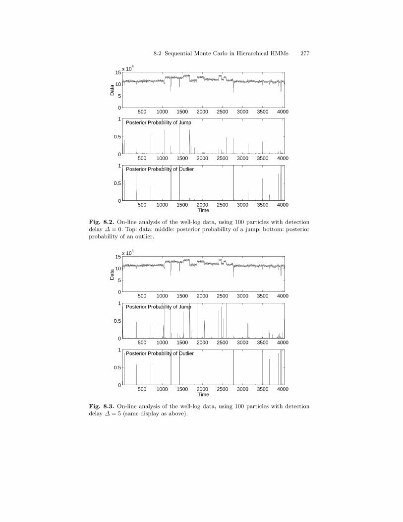
8.2 Sequential Monte Carlo in Hierarchical HMMs 277

500 1000 1500 2000 2500 3000 3500 40000

5

10

15x 10

4

Dat

a

500 1000 1500 2000 2500 3000 3500 40000

0.5

1Posterior Probability of Jump

500 1000 1500 2000 2500 3000 3500 40000

0.5

1

Time

Posterior Probability of Outlier

Fig. 8.2. On-line analysis of the well-log data, using 100 particles with detectiondelay ∆ = 0. Top: data; middle: posterior probability of a jump; bottom: posteriorprobability of an outlier.

500 1000 1500 2000 2500 3000 3500 40000

5

10

15x 10

4

Dat

a

500 1000 1500 2000 2500 3000 3500 40000

0.5

1Posterior Probability of Jump

500 1000 1500 2000 2500 3000 3500 40000

0.5

1

Time

Posterior Probability of Outlier

Fig. 8.3. On-line analysis of the well-log data, using 100 particles with detectiondelay ∆ = 5 (same display as above).

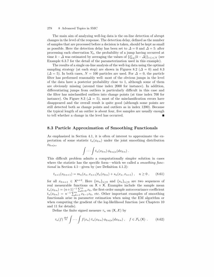
278 8 Advanced Topics in SMC

The main aim of analyzing well-log data is the on-line detection of abruptchanges in the level of the response. The detection delay, defined as the numberof samples that are processed before a decision is taken, should be kept as smallas possible. Here the detection delay has been set to ∆ = 0 and ∆ = 5: afterprocessing each observation Yk, the probability of a jump having occurred attime k−∆ was estimated by averaging the values of ξi0:k(k−∆)1≤i≤N (seeExample 6.3.7 for the detail of the parameterization used in this example).

The results of a single on-line analysis of the well-log data using the optimalsampling strategy (at each step) are shown in Figures 8.2 (∆ = 0) and 8.3(∆ = 5). In both cases, N = 100 particles are used. For ∆ = 0, the particlefilter has performed reasonably well: most of the obvious jumps in the levelof the data have a posterior probability close to 1, although some of themare obviously missing (around time index 2000 for instance). In addition,differentiating jumps from outliers is particularly difficult in this case andthe filter has misclassified outliers into change points (at time index 700 forinstance). On Figure 8.3 (∆ = 5), most of the misclassification errors havedisappeared and the overall result is quite good (although some points arestill detected both as change points and outliers as in index 1200). Becausethe typical length of an outlier is about four, five samples are usually enoughto tell whether a change in the level has occurred.

8.3 Particle Approximation of Smoothing Functionals

As emphasized in Section 4.1, it is often of interest to approximate the ex-pectation of some statistic tn(x0:n) under the joint smoothing distributionφ0:n|n, ∫

· · ·∫tn(x0:n)φ0:n|n(dx0:n) .

This difficult problem admits a computationally simpler solution in caseswhere the statistic has the specific form—which we called a smoothing func-tional in Section 4.1—given by (see Definition 4.1.2):

tn+1(x0:n+1) = mn(xn, xn+1)tn(x0:n) + sn(xn, xn+1) , n ≥ 0 , (8.61)

for all x0:n+1 ∈ Xn+2. Here mnn≥0 and snn≥0 are two sequences ofreal measurable functions on X × X. Examples include the sample meantn(x0:n) = (n+1)−1

∑nk=0 xk, the first-order sample autocovariance coefficient

tn(x0:n) = n−1∑nk=1 xk−1xk, etc. Other important examples of smoothing

functionals arise in parameter estimation when using the EM algorithm orwhen computing the gradient of the log-likelihood function (see Chapters 10and 11 for details).

Define the finite signed measure τn on (X,X ) by

τn(f) def=∫· · ·∫f(xn) tn(x0:n)φ0:n|n(dx0:n) , f ∈ Fb (X) . (8.62)

8.3 Particle Approximation of Smoothing Functionals 279

Note that by construction, τn(X) = φ0:n|n(tn), that is, the quantity of inter-est. By Proposition 4.1.3, the measures τnn≥0 may be updated recursivelyaccording to

τ0(f) = ν(g0)−1∫f(x0) t0(x0)g0(x0) ν(dx0)

and

τn+1(f) = c−1n+1

∫∫f(xn+1)

[τn(dxn)Q(xn, dxn+1)gn+1(xn+1)mn(xn, xn+1)

+ φn(dxn)Q(xn, dxn+1)gn+1(xn+1)sn(xn, xn+1)], (8.63)

where the normalizing constant cn+1 is given by (3.22) as cn+1 = φnQgn+1.It is easily seen that τn is absolutely continuous with respect to the filteringmeasure φn. Hence (8.63) may be rewritten as

τn+1(f) =∫∫

f(xn+1)×dτndφn

(xn)mn(xn, xn+1) + sn(xn, xn+1)φn:n+1|n+1(dxn:n+1) . (8.64)

In SISR algorithms, the joint smoothing distribution φ0:n+1|n+1 at time n+1 isapproximated by a set ξi0:n+11≤i≤N of particles with associated importanceweights ωin+11≤i≤N . Due to the sequential update of the particle trajecto-ries, there exist indices I1

n+1, . . . , INn+1 (see Algorithm 7.3.4) such that

ξi0:n+1 = (ξIin+10:n , ξin+1) ,

meaning that the first n + 1 coordinates of the path are simply copied fromthe previous generation of particles. Because τn is absolutely continuous withrespect to φn for any n, it seems reasonable to approximate τn using the samesystem of particles as that used to approximate φn. That is, for any n weapproximate τn by

τn =N∑i=1

ωin∑Nj=1 ω

jn

γinδξin , (8.65)

where γin, i = 1, . . . , N , are signed weights. Such approximations have beenconsidered in different settings by Cappe (2001a), Cerou et al. (2001), Doucetand Tadic (2003), and Fichou et al. (2004). This approximation of τn yieldsthe following estimator of φ0:n|n(tn) = τn(X):

φ0:n|n(tn) =N∑i=1

ωin∑Nj=1 ω

jn

γin . (8.66)

280 8 Advanced Topics in SMC

The two measures τn and φn have the same support, which implies thatτn is absolutely continuous with respect to φn; in addition, for any x ∈ξ1n, . . . , ξ

Nn ,

dτn

dφn(x) =

∑j∈In(x) ω

jnγ

jn∑

j∈In(x) ωjn

, (8.67)

where In(x) def= j = 1, . . . , N : ξjn = x. In cases where there are no ties (allparticle locations are distinct), we simply have

dτn

dφn(ξin) = γin . (8.68)

To derive a recursive approximation of τn, it is only needed to derive up-date equations for the signed weights γin. Plugging the particle approximationφn:n+1|n+1 ∝

∑Ni=1 ω

in+1δξin:n+1

of the retrospective smoothing distributionφn:n+1|n+1 into the update equation (8.64) yields the following approxima-tion of the measure τn+1:

N∑i=1

ωin+1∑Nj=1 ω

jn+1

dτndφn

(ξIin+1n )mn(ξ

Iin+1n , ξin+1) + sn(ξ

Iin+1n , ξin+1)

δξin+1

.

(8.69)Using the approximation (8.68) of dτn

dφn(ξjn), the latter relation suggests the

following recursion for the weights γin1≤i≤N :

γi0 = t0(ξi0) , (8.70)

γin+1 = γIin+1n mn(ξ

Iin+1n , ξin+1) + sn(ξ

Iin+1n , ξin+1) . (8.71)

This relation, originally derived by Cappe (2001a)2, is computationally at-tractive because the approximation uses the same set particles and weightsas those used to approximate the filtering distribution; only the incrementalsigned weights need to be computed recursively. Also, it mimics the exactrecursion for τn and therefore seems like a good way to approximate thissequence of measures.

To get a better understanding of the behavior of the algorithm, wewill derive the recursion (8.71) from a different (admittedly more elemen-tary) perspective. The sequential importance sampling approximation of thejoint smoothing distribution φ0:n|n amounts to approximate, for any statistictn(x0:n), φ0:n|n(tn) by

φ0:n|n(tn) =N∑i=1

ωin∑Nj=1 ω

jn

tn(ξi0:n) . (8.72)

2The recursion obtained by Cerou et al. (2001) is based on a very differentargument but turns out to be equivalent in the case where the functional of interestcorresponds to the gradient of the log-likelihood function (see Section 10.2.4 fordetails).

8.3 Particle Approximation of Smoothing Functionals 281

If the statistic tn is a smoothing functional as defined in (8.61), this quan-tity can be evaluated sequentially so that storing the whole particle paths isavoided. Denote by tin1≤i≤N the current value of the smoothing functionaltn along the particle path ξi0:n: tin = tn(ξi0:n). This quantity may be updatedaccording to the recursion ti0 = t0(ξi0) and

tin+1 = tIin+1n mn(ξ

Iin+1n , ξin+1) + sn(ξ

Iin+1n , ξin+1), i = 1, . . . , N . (8.73)

Perhaps surprisingly, because the two approximations have been derivedfrom two different perspectives, (8.73) and (8.71) are identical. This meansthat both equations are recursive ways to compute the approximation (8.72)of expectations with respect to the joint smoothing distribution. The sec-ond reasoning, which led to recursion (8.73), however, raises some concernabout the practical use of this approximation. Because the path particles(ξi0:n, ω

in)1≤i≤N are targeted to approximate a probability distribution over

the space Xn+1, whose dimension grows with n, it is to be expected that thecurse of dimensionality can only be fought by increasing the number N of pathparticles as n increases (Del Moral, 2004). A worst case analysis suggests thatthe number N of path particles should grow exponentially with n, which isof course unrealistic. This assertion should however be taken with some carebecause we are in general interested only in low-dimensional statistical sum-maries of the particle paths. Hence, the situation usually is more contrasted,as illustrated below on an example.

Example 8.3.1. We consider here the stochastic volatility model of Exam-ple 7.2.5:

Xk+1 = φXk + σUk , Uk ∼ N(0, 1) ,Yk = β exp(Xk/2)Vk , Vk ∼ N(0, 1) .

Here the observations Ykk≥0 are the log-returns, Xkk≥0 is the log-volatility, and Ukk≥0 and Vkk≥0 are independent sequences of standardwhite Gaussian noise. We use the SISR algorithm with systematic resamplingand instrumental kernel being a t-distribution with 5 degrees of freedom andmode and scale adjusted to the mode and curvature of the optimal instru-mental kernel (see Example 7.2.5). We consider the daily log-returns, thatis, the difference of the log of the series, on the British pound/US dollar ex-change rate from October, 1 1981, to June, 28 1985 (the data is scaled by100 and mean-corrected—see Kim et al., 1998, and Shephard and Pitt, 1997for details). The number of samples is n = 945, and we used the stochasticvolatility model with parameters φ = 0.975, β = 0.63, and σ = 0.16; theseare the maximum likelihood estimates reported by Sandmann and Koopman(1998) on this data set.

The path particles after 70 iterations are plotted in Figure 8.4. The figureclearly shows that the selection mechanism implies that for any given timeindex k ≤ n, the number of ancestors, at that time, of the particle trajectories

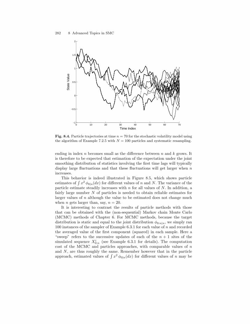
282 8 Advanced Topics in SMC

0 10 20 30 40 50 60 70−1

−0.5

0

0.5

1

1.5

2

Time Index

Sta

te V

alue

Fig. 8.4. Particle trajectories at time n = 70 for the stochastic volatility model usingthe algorithm of Example 7.2.5 with N = 100 particles and systematic resampling.

ending in index n becomes small as the difference between n and k grows. Itis therefore to be expected that estimation of the expectation under the jointsmoothing distribution of statistics involving the first time lags will typicallydisplay large fluctuations and that these fluctuations will get larger when nincreases.

This behavior is indeed illustrated in Figure 8.5, which shows particleestimates of

∫x2 φ0|n(dx) for different values of n and N . The variance of the

particle estimate steadily increases with n for all values of N . In addition, afairly large number N of particles is needed to obtain reliable estimates forlarger values of n although the value to be estimated does not change muchwhen n gets larger than, say, n = 20.

It is interesting to contrast the results of particle methods with thosethat can be obtained with the (non-sequential) Markov chain Monte Carlo(MCMC) methods of Chapter 6. For MCMC methods, because the targetdistribution is static and equal to the joint distribution φ0:n|n, we simply ran100 instances of the sampler of Example 6.3.1 for each value of n and recordedthe averaged value of the first component (squared) in each sample. Here a“sweep” refers to the successive updates of each of the n + 1 sites of thesimulated sequence Xi

0:n (see Example 6.3.1 for details). The computationcost of the MCMC and particles approaches, with comparable values of nand N , are thus roughly the same. Remember however that in the particleapproach, estimated values of

∫x2 φ0|n(dx) for different values of n may be

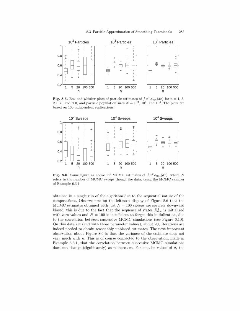
8.3 Particle Approximation of Smoothing Functionals 283

1 5 20 100 5000.2

0.4

0.6

0.8

1102 Particles

n 1 5 20 100 500

103 Particles

n 1 5 20 100 500

104 Particles

n

Fig. 8.5. Box and whisker plots of particle estimates of∫x2 φ0|n(dx) for n = 1, 5,

20, 30, and 500, and particle population sizes N = 102, 103, and 104. The plots arebased on 100 independent replications.

1 5 20 100 5000.2

0.4

0.6

0.8

1102 Sweeps

n 1 5 20 100 500

103 Sweeps

n 1 5 20 100 500

104 Sweeps

n

Fig. 8.6. Same figure as above for MCMC estimates of∫x2 φ0|n(dx), where N

refers to the number of MCMC sweeps though the data, using the MCMC samplerof Example 6.3.1.

obtained in a single run of the algorithm due to the sequential nature of thecomputations. Observe first on the leftmost display of Figure 8.6 that theMCMC estimates obtained with just N = 100 sweeps are severely downwardbiased: this is due to the fact that the sequence of states X1

0:n is initializedwith zero values and N = 100 is insufficient to forget this initialization, dueto the correlation between successive MCMC simulations (see Figure 6.10).On this data set (and with those parameter values), about 200 iterations areindeed needed to obtain reasonably unbiased estimates. The next importantobservation about Figure 8.6 is that the variance of the estimate does notvary much with n. This is of course connected to the observation, made inExample 6.3.1, that the correlation between successive MCMC simulationsdoes not change (significantly) as n increases. For smaller values of n, the

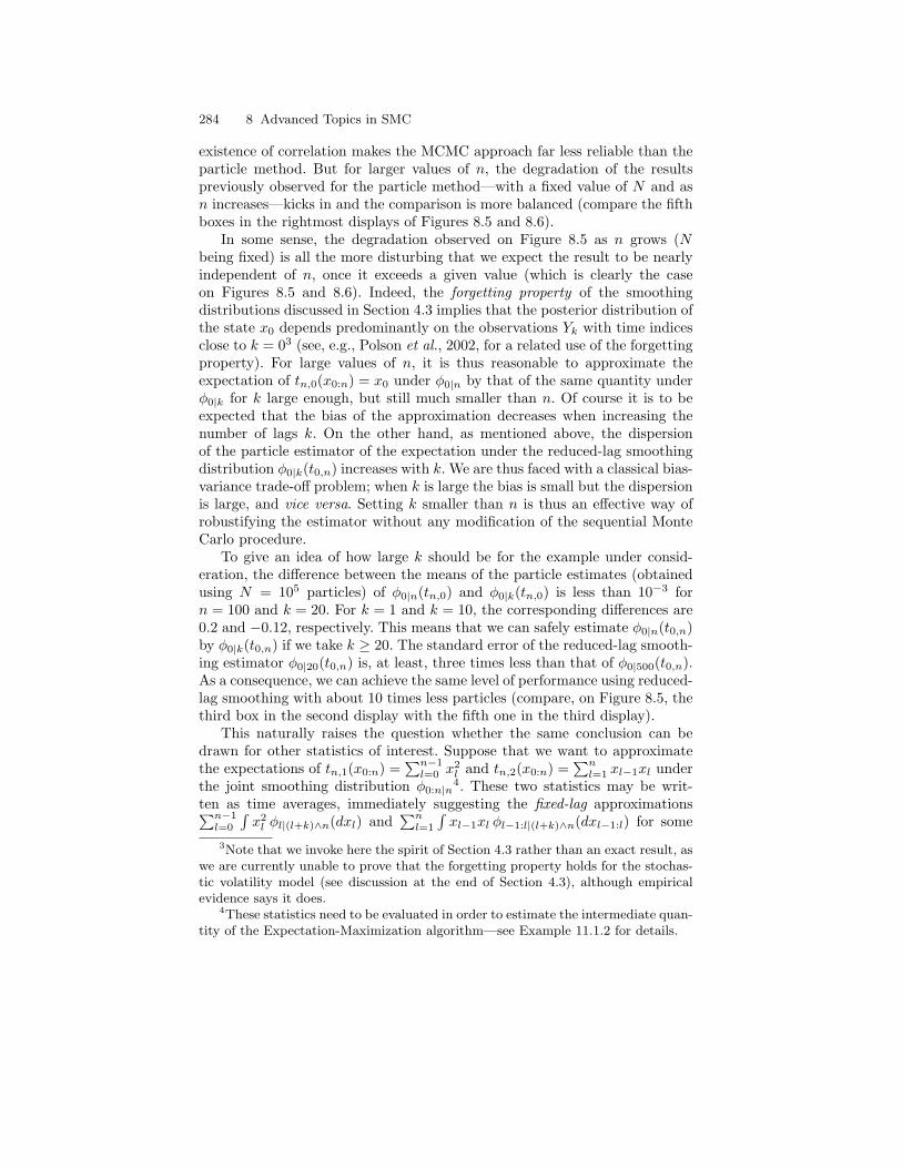
284 8 Advanced Topics in SMC

existence of correlation makes the MCMC approach far less reliable than theparticle method. But for larger values of n, the degradation of the resultspreviously observed for the particle method—with a fixed value of N and asn increases—kicks in and the comparison is more balanced (compare the fifthboxes in the rightmost displays of Figures 8.5 and 8.6).

In some sense, the degradation observed on Figure 8.5 as n grows (Nbeing fixed) is all the more disturbing that we expect the result to be nearlyindependent of n, once it exceeds a given value (which is clearly the caseon Figures 8.5 and 8.6). Indeed, the forgetting property of the smoothingdistributions discussed in Section 4.3 implies that the posterior distribution ofthe state x0 depends predominantly on the observations Yk with time indicesclose to k = 03 (see, e.g., Polson et al., 2002, for a related use of the forgettingproperty). For large values of n, it is thus reasonable to approximate theexpectation of tn,0(x0:n) = x0 under φ0|n by that of the same quantity underφ0|k for k large enough, but still much smaller than n. Of course it is to beexpected that the bias of the approximation decreases when increasing thenumber of lags k. On the other hand, as mentioned above, the dispersionof the particle estimator of the expectation under the reduced-lag smoothingdistribution φ0|k(t0,n) increases with k. We are thus faced with a classical bias-variance trade-off problem; when k is large the bias is small but the dispersionis large, and vice versa. Setting k smaller than n is thus an effective way ofrobustifying the estimator without any modification of the sequential MonteCarlo procedure.

To give an idea of how large k should be for the example under consid-eration, the difference between the means of the particle estimates (obtainedusing N = 105 particles) of φ0|n(tn,0) and φ0|k(tn,0) is less than 10−3 forn = 100 and k = 20. For k = 1 and k = 10, the corresponding differences are0.2 and −0.12, respectively. This means that we can safely estimate φ0|n(t0,n)by φ0|k(t0,n) if we take k ≥ 20. The standard error of the reduced-lag smooth-ing estimator φ0|20(t0,n) is, at least, three times less than that of φ0|500(t0,n).As a consequence, we can achieve the same level of performance using reduced-lag smoothing with about 10 times less particles (compare, on Figure 8.5, thethird box in the second display with the fifth one in the third display).

This naturally raises the question whether the same conclusion can bedrawn for other statistics of interest. Suppose that we want to approximatethe expectations of tn,1(x0:n) =

∑n−1l=0 x

2l and tn,2(x0:n) =

∑nl=1 xl−1xl under

the joint smoothing distribution φ0:n|n4. These two statistics may be writ-

ten as time averages, immediately suggesting the fixed-lag approximations∑n−1l=0

∫x2l φl|(l+k)∧n(dxl) and

∑nl=1

∫xl−1xl φl−1:l|(l+k)∧n(dxl−1:l) for some

3Note that we invoke here the spirit of Section 4.3 rather than an exact result, aswe are currently unable to prove that the forgetting property holds for the stochas-tic volatility model (see discussion at the end of Section 4.3), although empiricalevidence says it does.

4These statistics need to be evaluated in order to estimate the intermediate quan-tity of the Expectation-Maximization algorithm—see Example 11.1.2 for details.

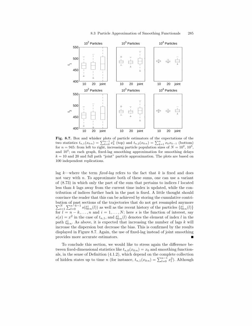
8.3 Particle Approximation of Smoothing Functionals 285

10 20 joint400

450

500

550102 Particles

t 1

10 20 joint

103 Particles

10 20 joint

104 Particles

10 20 joint400

450

500

550102 Particles

t 2

10 20 joint

103 Particles

10 20 joint

104 Particles

Fig. 8.7. Box and whisker plots of particle estimators of the expectations of thetwo statistics tn,1(x0:n) =

∑n−1k=0 x

2k (top) and tn,2(x0:n) =

∑nk=1 xkxk−1 (bottom)

for n = 945: from left to right, increasing particle population sizes of N = 102, 103,and 104; on each graph, fixed-lag smoothing approximation for smoothing delaysk = 10 and 20 and full path “joint” particle approximation. The plots are based on100 independent replications.

lag k—where the term fixed-lag refers to the fact that k is fixed and doesnot vary with n. To approximate both of these sums, one can use a variantof (8.73) in which only the part of the sum that pertains to indices l locatedless than k lags away from the current time index is updated, while the con-tribution of indices further back in the past is fixed. A little thought shouldconvince the reader that this can be achieved by storing the cumulative contri-bution of past sections of the trajectories that do not get resampled anymore∑Ni=1

∑n−k−1l=0 s(ξi0:n(l)) as well as the recent history of the particles ξi0:n(l)

for l = n − k, . . . , n and i = 1, . . . , N ; here s is the function of interest, says(x) = x2 in the case of tn,1, and ξi0:n(l) denotes the element of index l in thepath ξi0:n. As above, it is expected that increasing the number of lags k willincrease the dispersion but decrease the bias. This is confirmed by the resultsdisplayed in Figure 8.7. Again, the use of fixed-lag instead of joint smoothingprovides more accurate estimators.

To conclude this section, we would like to stress again the difference be-tween fixed-dimensional statistics like tn,0(x0:n) = x0 and smoothing function-als, in the sense of Definition (4.1.2), which depend on the complete collectionof hidden states up to time n (for instance, tn,1(x0:n) =

∑n−1l=0 x

2l ). Although

286 8 Advanced Topics in SMC

the latter case does seem to be more challenging, the averaging effect due ton should not be underestimated: even crude approximations of the individualterms, say

∫x2l φl|n(dxl) in the case of tn,1, may add up to provide a reliable

approximation of the conditional expectation of tn,1. In our experience, thestrategy discussed above is usually successful with rather moderate values ofthe lag k and the number N of particles, as will be illustrated in Chapter 11.In the case of fixed-dimensional statistics, more elaborate smoothing algo-rithms may be more recommendable, particularly in situations where relyingon forgetting properties might be questionable (Kitagawa, 1996; Fong et al.,2002; Briers et al., 2004).

9

Analysis of Sequential Monte Carlo Methods

The previous chapters have described many algorithms to approximate pre-diction, filtering, and smoothing distributions. The development of these al-gorithms was motivated mainly on heuristic grounds, and the validity of theseapproximations is of course a question of central interest. In this chapter, weanalyze these methods, mainly from an asymptotic perspective. That is, westudy the behavior of the estimators in situations where the number of par-ticles gets large. Asymptotic analysis provides approximations that in manycircumstances have proved to be relatively robust. Most importantly, asymp-totic arguments provide insights in the sampling methodology by verifyingthat the procedures are sensible, providing a framework for comparing com-peting procedures, and providing understanding of the impact of differentoptions (choice of importance kernel, etc.) on the overall performance of thesamplers.

9.1 Importance Sampling

9.1.1 Unnormalized Importance Sampling

Let (X,X ) be a measurable space. Define on (X,X ) two probability distribu-tions: the target distribution µ and the instrumental distribution ν.

Assumption 9.1.1. The target distribution µ is absolutely continuous withrespect to the instrumental distribution ν, µ ν, and dµ/dν > 0 ν-a.s.

Let f be a real-valued measurable function on X such that µ(|f |) =∫|f | dµ <

∞. Denote by ξ1, ξ2, . . . an i.i.d. sample from ν and consider the estimator

µISν,N (f) =

1N

N∑i=1

f(ξi)dµ

dν(ξi) . (9.1)

288 9 Analysis of SMC Methods

Because this estimator is the sample average of independent random vari-ables, there is a range of results to assess the accuracy of µIS

ν,N (f) as anestimator of µ(f). Some of these results are asymptotic in nature, like thelaw of large numbers (LLN) and the central limit theorem (CLT). It is alsopossible to derive non-asymptotic bounds like Berry-Esseen bounds, boundson error moments E |µIS

ν,N (f)−µ(f)|p for some p > 0 or on the tail probabilityP(|µISν,N (f)− µ(f)| ≥ ε

). Instead of covering the full scale of results that can

be derived, we establish for the different algorithms presented in the previouschapter a law of large numbers, a central limit theorem, and deviation bounds.

A direct application of the LLN and of the CLT yields the following result.

Theorem 9.1.2. Let f be a real measurable function such that µ(|f |) < ∞and |f |µ |f |ν, and let ξ1, ξ2, . . . be a sequence of i.i.d. random variablesfrom ν. Then the unnormalized importance sampling estimator µIS

ν,N (f) givenby (9.1) is strongly consistent, limN→∞ µIS

ν,N (f) = µ(f) a.s.Assume in addition that∫

f2

[dµ

dν

]2

dν <∞ . (9.2)

Then µISν,N (f) is asymptotically Gaussian,

√N(µIS

ν,N (f)− µ(f)) D−→ N(

0,Varν

(fdµ

dν

))as N →∞ ,

where Varν(f dµdν

)is given by

Varν

(fdµ

dν

)=∫ [

fdµ

dν− µ(f)

]2

dν .

Obviously, while the importance sampling construction (9.1) is universal,the performance of the importance sampling estimator depends heavily onthe relation between the target distribution µ, the instrumental distributionν, and the function f . It is also worthwhile to note that for a given functionf , it is most often possible to find a distribution ν that yields an estimatewith a lower variance than when using the Monte Carlo method, that is,taking ν = µ. In some situations the improvements can be striking: this is inparticular the case where the function f is non-zero only for values that arein the tails of the target distribution µ, a situation that occurs for instancewhen estimating the probability of rare events. The basic idea is to choose theimportance distribution ν so that it generates values that are in the regionwhere the integrand f dµdν is large, as this region is where the most importantcontributions are made to the value of the integral.

Notice that

Varν

(fdµ

dν

)= [µ(f)]2 ν

[(|f |dµ/dνµ(|f |)

− 1)2],

9.1 Importance Sampling 289

where the second factor on the right-hand side is the chi-square distancebetween the densities 1 and |f |dµdν /µ(|f |) under ν. This factor is of coursein general unknown, but may be estimated consistently by computing the(squared) coefficient of variation CV2

N , see (7.35), of the importance weightsωi = |f(ξi)|dµdν (ξi), i = 1, . . . , N .

Poor selection of the instrumental distribution can induce large variationsin the importance weights dµ/dν and thus unreliable approximations of µ(f).In many settings, an inappropriate choice of the instrumental distributionmight lead to an estimator (9.1) whose variance is infinite (and which thereforedoes not satisfy the assumptions of the CLT). Here is a simple example of thisbehavior.

Example 9.1.3 (Importance Sampling with Cauchy and GaussianVariables). In this example, the target µ = C(0, 1) is a standard Cauchydistribution, and the instrumental distribution ν = N(0, 1) is a standard Gaus-sian distribution. The importance weight function, given by

dµ

dν(x) =

√2π

exp(x2/2)π (1 + x2)

,

is obviously badly behaved. In particular

1√2π

∫ ∞−∞

[dµ

dν(x)]2

exp(−x2/2) dx =∞ .

Figure 9.1 illustrates the poor performance of the associated importance sam-pling estimator for the function f(x) = exp(−|x|). We have displayed thequantile-quantile plot of the sample quantiles of the unnormalized IS estimatorµISν,N (f), obtained from m = 500 independent Monte Carlo experiments, ver-

sus the quantiles of a standard normal distribution. In the left panel N =100and in the right panel N =1,000. The quantile-quantile plot shows deviationsfrom the normal distribution in both the lower and the upper tail for bothN =100 and N =1,000, indicating that the distribution of µIS

ν,N (f) does notconverge in the limit to a Gaussian distribution.

Example 9.1.4. We now switch the roles of the target and instrumental dis-tributions, taking µ = N(0, 1) and ν = C(0, 1). The importance weight isbounded by

√2π/e, and this time Theorem 9.1.2 can be applied. Quantile-

quantile plots of the sample quantiles of the unnormalized IS estimatorµISν,N (f) are shown in Figure 9.2. The fit is good, even when the sample size

is small (N = 100). It is worthwhile to investigate the impact of the choiceof the scale of the Cauchy distribution. Assume now that ν = C(0, σ) whereσ > 0 is the scale parameter. The importance weight function is bounded by

√2πeσ eσ

2/2 , σ <√

2 ,

σ√π/2 , σ ≥

√2 .

(9.3)

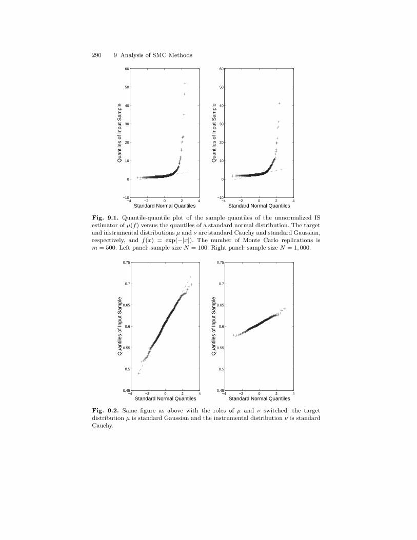
290 9 Analysis of SMC Methods

−4 −2 0 2 4−10

0

10

20

30

40

50

60

Standard Normal Quantiles

Qua

ntile

s of

Inpu

t Sam

ple

−4 −2 0 2 4−10

0

10

20

30

40

50

60

Standard Normal Quantiles

Qua

ntile

s of

Inpu

t Sam

ple

Fig. 9.1. Quantile-quantile plot of the sample quantiles of the unnormalized ISestimator of µ(f) versus the quantiles of a standard normal distribution. The targetand instrumental distributions µ and ν are standard Cauchy and standard Gaussian,respectively, and f(x) = exp(−|x|). The number of Monte Carlo replications ism = 500. Left panel: sample size N = 100. Right panel: sample size N = 1, 000.

−4 −2 0 2 40.45

0.5

0.55

0.6

0.65

0.7

0.75

Standard Normal Quantiles

Qua

ntile

s of

Inpu

t Sam

ple

−4 −2 0 2 40.45

0.5

0.55

0.6

0.65

0.7

0.75

Standard Normal Quantiles

Qua

ntile

s of

Inpu

t Sam

ple

Fig. 9.2. Same figure as above with the roles of µ and ν switched: the targetdistribution µ is standard Gaussian and the instrumental distribution ν is standardCauchy.

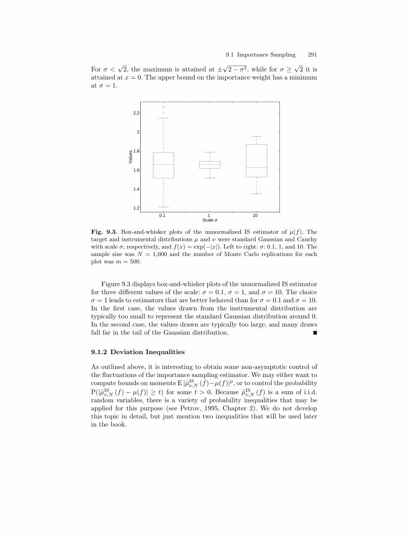
9.1 Importance Sampling 291

For σ <√

2, the maximum is attained at ±√

2− σ2, while for σ ≥√

2 it isattained at x = 0. The upper bound on the importance weight has a minimumat σ = 1.

0.1 1 10

1.2

1.4

1.6

1.8

2

2.2

Val

ues

Scale σ

Fig. 9.3. Box-and-whisker plots of the unnormalized IS estimator of µ(f). Thetarget and instrumental distributions µ and ν were standard Gaussian and Cauchywith scale σ, respectively, and f(x) = exp(−|x|). Left to right: σ: 0.1, 1, and 10. Thesample size was N = 1,000 and the number of Monte Carlo replications for eachplot was m = 500.

Figure 9.3 displays box-and-whisker plots of the unnormalized IS estimatorfor three different values of the scale: σ = 0.1, σ = 1, and σ = 10. The choiceσ = 1 leads to estimators that are better behaved than for σ = 0.1 and σ = 10.In the first case, the values drawn from the instrumental distribution aretypically too small to represent the standard Gaussian distribution around 0.In the second case, the values drawn are typically too large, and many drawsfall far in the tail of the Gaussian distribution.

9.1.2 Deviation Inequalities

As outlined above, it is interesting to obtain some non-asymptotic control ofthe fluctuations of the importance sampling estimator. We may either want tocompute bounds on moments E |µIS

ν,N (f)−µ(f)|p, or to control the probabilityP(|µIS

ν,N (f) − µ(f)| ≥ t) for some t > 0. Because µISν,N (f) is a sum of i.i.d.

random variables, there is a variety of probability inequalities that may beapplied for this purpose (see Petrov, 1995, Chapter 2). We do not developthis topic in detail, but just mention two inequalities that will be used laterin the book.

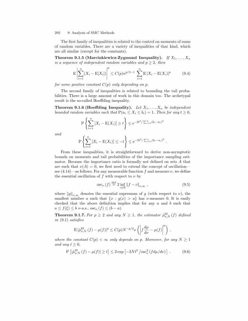
292 9 Analysis of SMC Methods

The first family of inequalities is related to the control on moments of sumsof random variables. There are a variety of inequalities of that kind, whichare all similar (except for the constants).

Theorem 9.1.5 (Marcinkiewicz-Zygmund Inequality). If X1, . . . , Xn

is a sequence of independent random variables and p ≥ 2, then

E

∣∣∣∣∣n∑i=1

(Xi − E[Xi])

∣∣∣∣∣p

≤ C(p)np/2−1n∑i=1

E |Xi − E(Xi)|p (9.4)

for some positive constant C(p) only depending on p.

The second family of inequalities is related to bounding the tail proba-bilities. There is a large amount of work in this domain too. The archetypalresult is the so-called Hoeffding inequality.

Theorem 9.1.6 (Hoeffding Inequality). Let X1, . . . , Xn be independentbounded random variables such that P(ai ≤ Xi ≤ bi) = 1. Then for any t ≥ 0,

P

n∑i=1

[Xi − E(Xi)] ≥ t

≤ e−2t2/

∑ni=1(bi−ai)2

and

P

n∑i=1

[Xi − E(Xi)] ≤ −t

≤ e−2t2/

∑ni=1(bi−ai)2

.

From these inequalities, it is straightforward to derive non-asymptoticbounds on moments and tail probabilities of the importance sampling esti-mator. Because the importance ratio is formally not defined on sets A thatare such that ν(A) = 0, we first need to extend the concept of oscillation—see (4.14)—as follows. For any measurable function f and measure ν, we definethe essential oscillation of f with respect to ν by

oscν (f) def= 2 infc∈R‖f − c‖ν,∞ , (9.5)

where ‖g‖ν,∞ denotes the essential supremum of g (with respect to ν), thesmallest number a such that x : g(x) > a has ν-measure 0. It is easilychecked that the above definition implies that for any a and b such thata ≤ f(ξ) ≤ b ν-a.s., oscν (f) ≤ (b− a).

Theorem 9.1.7. For p ≥ 2 and any N ≥ 1, the estimator µISν,N (f) defined

in (9.1) satisfies

E |µISν,N (f)− µ(f)|p ≤ C(p)N−p/2ν

(∣∣∣∣f dµdν − µ(f)∣∣∣∣p) ,

where the constant C(p) < ∞ only depends on p. Moreover, for any N ≥ 1and any t ≥ 0,

P[|µISν,N (f)− µ(f)| ≥ t

]≤ 2 exp

[−2Nt2

/osc2

ν (fdµ/dν)]. (9.6)

9.1 Importance Sampling 293

9.1.3 Self-normalized Importance Sampling Estimator

When the normalizing constant of the target distribution µ is unknown, it iscustomary to use the self-normalized form of the importance sampling esti-mator,

µISν,N (f) =

∑Ni=1 f(ξi)dµdν (ξi)∑N

i=1dµdν (ξi)

. (9.7)

This quantity is obviously free from any scale factor in dµ/dν. The propertiesof this estimator are of course closely related to those of the unnormalizedimportance sampling estimator.

9.1.3.1 Consistency and Asymptotic Normality

Theorem 9.1.8. Let f be a measurable function such that µ(|f |) < ∞. As-sume that µ ν and let ξ1, ξ2, . . . , be an i.i.d. sequence with distribution ν.Then

µISν,N (f) a.s.−→ µ(f) as N →∞ .

Assume in addition that f satisfies∫[1 + f2]

[dµ

dν

]2

dν <∞ . (9.8)

Then the sequence of estimators µISν,N (f) is asymptotically Gaussian,

√N[µISν,N (f)− µ(f)

] D−→ N(0, σ2(ν, f)

)as N →∞ ,

where

σ2(ν, f) =∫ [

dµ

dν

]2

[f − µ(f)]2dν . (9.9)

Proof. Strong consistency follows from

N−1N∑i=1

f(ξi)dµ

dν(ξi) a.s.−→ µ(f) and N−1

N∑i=1

dµ

dν(ξi) a.s.−→ 1 .

Write

√N[µISν,N (f)− µ(f)

]=N−1/2

∑Ni=1

dµdν (ξi)

[f(ξi)− µ(f)

]N−1

∑Ni=1

dµdν (ξi)

.

By the central limit theorem, the numerator of the right-hand side aboveconverges weakly to N(0, σ2(ν, f)) as N → ∞, with σ2(ν, f) given by (9.9),and as noted above the corresponding denominator converges a.s. to 1. Thesecond part of the theorem then follows by Slutsky’s theorem (Billingsley,1995). ut

294 9 Analysis of SMC Methods

9.1.3.2 Deviation Inequalities

Assessing deviance bounds for (9.7) is not a trivial task, because both thenumerator and the denominator of µIS

ν,N (f) are random. The following ele-mentary lemma plays a key role in deriving such bounds.

Lemma 9.1.9. Let f be a measurable function and assume that µ ν. Letc be a real constant and define f = f − c. Then

∣∣µISν,N (f)− µ(f)

∣∣ ≤ ∣∣∣∣∣ 1N

N∑i=1

[dµ

dν(ξi)f(ξi)− µ(f)

]∣∣∣∣∣+∥∥f∥∥

ν,∞

∣∣∣∣∣ 1N

N∑i=1

[dµ

dν(ξi)− 1

]∣∣∣∣∣ ν-a.s. (9.10)

Proof. First note that µISν,N (f) − µ(f) = µIS

ν,N

(f)− µ(f). Next consider the

decomposition

µISν,N

(f)− µ(f) =

1N

N∑i=1

[dµ

dν(ξi)(f(ξi)− µ(f))

]

+∑Ni=1

dµdν (ξi)f(ξi)∑N

i=1dµdν (ξi)

[1− 1

N

N∑i=1

dµ

dν(ξi)

].

Finally, use the triangle inequality and maximize over f(ξi) in the secondterm. ut

From this result we may obtain moment bounds using the Marcinkiewicz-Zygmund inequality or, under more stringent conditions, exponential boundson tail probabilities.

Theorem 9.1.10. Assume that ν [(dµ/dν)p] <∞ for some p ≥ 2. Then thereexists a constant C <∞ such that for any N ≥ 1 and measurable function f ,

E |µISν,N (f)− µ(f)|p ≤ CN−p/2 oscpν (f) . (9.11)

In addition, for any t ≥ 0,

P[|µISν,N (f)− µ(f)| ≥ t

]≤ 4 exp

[−8Nt2

/9 ‖dµ/dν‖2ν,∞ osc2

ν (f)]. (9.12)

Proof. The bound (9.11) is a direct consequence of Lemma 9.1.9 and theMarcinkiewicz-Zygmund inequality (Theorem 9.1.5). Note that by minimiz-ing over c in the right-hand side of (9.10), we may replace

∥∥f∥∥ν,∞ by

(1/2) oscν (f), which is done here.For the second part pick b ∈ (0, 1) and write, using Lemma 9.1.9,

9.2 Sampling Importance Resampling 295

P[|µISν,N (f)− µ(f)| ≥ t

]≤ P

[∣∣∣∣∣N∑i=1

(dµ

dν(ξi)f(ξi)− µ(f)

)∣∣∣∣∣ ≥ Nbt]

+ P

[∣∣∣∣∣N∑i=1

(dµ

dν(ξi)− 1

)∣∣∣∣∣ ≥ N(1− b)t/∥∥f∥∥

ν,∞

].

Next apply Hoeffding’s inequality (Theorem 9.1.6) to both terms on the right-hand side to obtain

P[|µISν,N (f)− µ(f)| ≥ t

]≤ 2 exp

−2Nb2t2

/osc2

ν

[(dµ/dν)f

]+ 2 exp

[−2N(1− b)2t2

/‖dµ/dν‖2ν,∞

∥∥f∥∥2

ν,∞

], (9.13)

where the fact that oscν (dµ/dν) ≤ ‖dµ/dν‖ν,∞ (as dµ/dν is positive) hasbeen used. Now note that when f is such that

∥∥f∥∥ν,∞ = (1/2) oscν (f),

oscν[(dµ/dν)f

]≤ ‖dµ/dν‖ν,∞ oscν (f). Hence to equate both terms on the

right-hand side of (9.13) we set b = 2/3 which gives (9.12). ut

9.2 Sampling Importance Resampling

9.2.1 The Algorithm

In this section, we study the sampling importance resampling (SIR) technique,introduced by Rubin (1987, 1988). It enables drawing an asymptotically inde-pendent sample ξ1, . . . , ξN from a target distribution µ. The method requiresthat we know an instrumental distribution ν satisfying µ ν and such thatthe Radon-Nikodym derivative dµ/dν is known up to a normalizing factor.Therefore either µ or ν, or both, may be known up to a normalizing constantonly. A tacit assumption is that sampling from the instrumental distributionν is doable.

The SIR method proceeds in two steps. In the sampling stage, we drawan i.i.d. sample ξ1, . . . , ξM from the instrumental distribution ν. The sizeM of this intermediate sample is usually taken to be larger, and sometimesmuch larger, than the size M of the final sample. In the resampling stage, wedraw a sample ξ1, . . . , ξM of size M from the instrumental sample ξ1, . . . , ξM .There are several ways of implementing this basic idea, the most obviousapproach being to sample with replacement with a probability of picking eachξi, i = 1, . . . ,M , that is proportional to its importance weight dµ

dν (ξi). Thatis, ξi = ξI

i

for i = 1, . . . , M , where I1, . . . , IM are conditionally independentgiven the instrumental sample and with distribution

P(I1 = i | ξ1, . . . , ξM ) =dµdν (ξi)∑Mj=1

dµdν (ξj)

.

296 9 Analysis of SMC Methods

For any measurable real-valued function f , we may associate to this samplean estimator µSIR

ν,M(f) of µ(f), defined as the Monte Carlo estimator of µ(f)

associated to the resampled particles ξ1, . . . , ξM ,

µSIRν,M

(f) =1M

M∑i=1

f(ξi) =1M

M∑i=1

N if(ξi) . (9.14)

HereN i is the total number of times that ξi was selected from the instrumentalsample. Thus (N1, . . . , NM ) have a multinomial distribution with

E[N i | ξ1, . . . , ξM ] = Mdµdν (ξi)∑Mj=1

dµdν (ξi)

, i = 1, . . . ,M .

The conditional expectation of the SIR estimate with respect to the instru-mental sample equals the (self-normalized) importance sampling estimatorprovided by this sample,

E[µSIRν,M

(f) | ξ1, . . . , ξM ] =M∑i=1

dµdν (ξi)∑Mi=1

dµdν (ξi)

f(ξi) .

The asymptotic analysis of the SIR estimator involves more sophisti-cated arguments however, because ξ1, . . . , ξM is not an i.i.d. sample fromµ. Nevertheless, for any measurable bounded real-valued function f on X andj = 1, . . . , M ,

E[f(ξj) | ξ1, . . . , ξM ] =M∑i=1

dµdν (ξi)∑Mj=1

dµdν (ξj)

f(ξi) P−→ µ(f) ,

where the convergence follows from Theorem 9.1.8. Because the conditionalexpectation on the left-hand side is bounded by ‖f‖∞, we can take expec-tations of both sides and appeal to dominated convergence to conclude thatE[f(ξj)]→ µ(f) as M →∞. This shows that, whereas marginally the ξi arenot distributed according to µ, the distribution of any ξi is asymptoticallycorrect in the sense that for any i, the marginal distribution of ξi convergesto the target distribution µ as M → ∞. In the same way, for any i 6= j andf, g ∈ Fb (X) we have

E[f(ξi)g(ξj)] = E[E[f(ξi)g(ξj) | ξ1, . . . , ξM ]]

= E[E[f(ξi) | ξ1, . . . , ξM ] E[g(ξj) | ξ1, . . . , ξM ]]

= E[µISν,M (f) µIS

ν,M (g)] .

Repeating the argument above shows that E[f(ξi)g(ξj)] → µ(f)µ(g). Thus,whereas the random variables ξi and ξj for i 6= j are not independent for any

9.2 Sampling Importance Resampling 297

given sample size M , they are asymptotically independent as the sample sizeM goes to infinity.

The estimation error µSIRν,M (f)− µ(f) can be decomposed into two terms,

µSIRν,M

(f)− µ(f) = µSIRν,M

(f)− µISν,M (f) + µIS

ν,M (f)− µ(f) . (9.15)

The first term on the right-hand side is the error associated with the approxi-mation of the importance sampling estimator µIS

ν,M (f) by its sampled versionµSIRν,M

(f). The second term is the error associated to the importance samplingestimator. To obtain asymptotic results, we now assume that the instrumen-tal and final sample sizes are non-decreasing sequences of integers, denoted byMN and MN, respectively, both diverging to infinity. As shown in Theo-rem 9.2.15, when µ(|f |) <∞, these two error terms go to zero and thereforeµSIRν,MN

(f) is a consistent estimator of µ(f).The next question to answer in the elementary asymptotic theory devel-

oped in this chapter is to find conditions upon which aNµSIRν,MN

(f) − µ(f)is asymptotically normal; here aN, the rate sequence, is a non-decreasingsequence of positive reals. Again we use the decomposition (9.15). First aconditional central limit theorem shows that, for any f ∈ L2(X, µ),

M1/2N

[µSIRν,MN

(f)− µISν,MN

(f)]

= M−1/2N

MN∑i=1

f(ξi)− E[f(ξi) | ξ1, . . . , ξMN ]

D−→ N (0,Varµ(f)) .

Note that N(0,Varµ(f)) is the limiting distribution of the plain Monte Carloestimator of µ(f) from an i.i.d. sample from µ. Theorem 9.1.8 shows that if(1 + f2)(dµ/dν)2 is ν-integrable, then

M1/2N

µISν,MN

(f)− µ(f) D−→ N

(0,Varν

dµ

dν[f − µ(f)]

).

The key result, shown in Theorem 9.2.15, is that M1/2N µSIR

ν,MN(f)−µIS

ν,MN(f)

and M1/2N µIS

ν,MN(f)− µ(f) are asymptotically independent.

In many circumstances, and in particular when studying the resamplingstep in sequential or iterative applications of the SIR algorithm (such as inthe sequential Monte Carlo framework), it is convenient to relax the condi-tions on the instrumental sample ξ1, . . . , ξM . In addition, it is of interest toconsider weighted samples (ξ1, ω1), . . . , (ξM , ωM ), where ωi are non-negative(importance) weights. We now proceed by introducing precise definitions andnotations and then present the main results.

9.2.2 Definitions and Notations

Let MNN≥0 be a sequence of positive integers. Throughout this section, weuse the word triangular array to refer to a system UN,i1≤i≤MN

of random

298 9 Analysis of SMC Methods

variables defined on a common probability space (Ω,F ,P) and organized asfollows:

U1,1 U1,2 . . . U1,M1

U2,1 U2,2 . . . . . . U2,M2

U3,1 U3,2 . . . . . . . . . U3,M3

......

......

.... . .

The row index N ranges over 1, 2, 3, . . . while the column index i ranges from 1to MN , where MN is a sequence of integers satisfying limN→∞MN

=∞. It willusually be the case that M1 < M2 < . . . ; hence the term triangular. It is notnecessary to assume this, however. It is not assumed that the random variableswithin each row are independent nor that they are identically distributed. Weassume nothing about the relation between the random variables on differentrows.

Let GNN≥0 be a sequence of sub-σ-fields of F . We say that a triangulararray UN,i1≤i≤MN

is measurable with respect to this sequence if for any Nthe random variables UN,1, . . . , UN,MN are GN -measurable. We say that thetriangular array UN,i1≤i≤MN

is conditionally independent given GN if forany N the random variables UN,1, . . . , UN,MN are conditionally independentgiven GN . The term conditionally i.i.d. given GN is defined in an entirelysimilar manner.

In the sequel, we will need a number of technical results regarding trian-gular arrays. To improve readability of the text, however, these results aregathered at the end of the chapter, in Section 9.5.1.

Definition 9.2.1 (Weighted Sample). A triangular array of random vari-ables (ξN,i, ωN,i)1≤i≤MN

is said to be a weighted sample if for any N ≥ 1,ωN,i ≥ 0 for i = 1, . . . ,MN and

∑MN

i=1 ωN,i > 0 a.s.

Let us now consider specifically the case when the variables ξN,i take val-ues in the space X. Assume that the weighted sample (ξN,i, ωN,i)1≤i≤MN

approximates the instrumental distribution ν in the sense that for any fin an appropriately defined class of functions, W−1

N

∑MN

i=1 ωN,if(ξN,i), with

WN =∑MN

i=1 ωN,i being the normalization factor, converges in an appropri-

ately defined sense to ν(f) as N tends to infinity. The most elementary wayto assess this convergence consists in requiring that W−1

N

∑MN

i=1 ωN,if(ξN,i)

converges to ν(f) in probability for functions f in some class C of real-valuedfunctions on X.

Definition 9.2.2 (Consistent Weighted Sample). The weighted sample(ξN,i, ωN,i)1≤i≤MN

is said to be a consistent for the probability measure νand the set C ⊆ L1(X, ν) if for any f ∈ C,

MN∑i=1

ωN,i∑MN

j=1 ωN,j

f(ξN,i

) P−→ ν(f) as N →∞ .

9.2 Sampling Importance Resampling 299

In order to obtain sensible results, we restrict our attention to classes of setsthat are sufficiently rich.

Definition 9.2.3 (Proper Set). A set C of real-valued measurable functionson X is said to be proper if the following conditions are satisfied.

(i) C is a linear space: for any f and g in C and reals α and β, αf+βg ∈ C.(ii) If |g| ∈ C and f is measurable with |f | ≤ |g|, then |f | ∈ C .

For any function f , define the positive and negative parts of it by

f+ def= f ∨ 0 and f−def= (−f) ∨ 0 ,

and note that f+ and f− are both dominated by |f |. Thus, if |f | ∈ C, thenf+ and f− both belong to C and so does f = f+ − f−. It is easily seen thatfor any p ≥ 0 and any measure µ on (X,X ), the set Lp(X, µ) is proper.

There are many different ways to obtain a consistent weighted sample.An i.i.d. sample ξN,i1≤i≤MN

with common distribution ν is consistent for(ν, L1(X, ν)

), and (ξN,i, dµdν (ξN,i)1≤i≤MN

is consistent for (µ,L1(X, µ)). Ofcourse, when dealing with such elementary situations, the use of triangulararrays can be avoided. Triangular arrays come naturally into play when consid-ering iterated applications of the SIR algorithm, as in sequential importancesampling techniques. In this case, the weighted sample (ξN,i, ωN,i1≤i≤MN

is the result of iterated applications of importance sampling, resampling, andpropagation steps. We study several examples of such situations later in thischapter.

The notion of sample consistency is weak but is in practice only moder-ately helpful, because it does not indicate the rate at which the estimatorW−1N

∑Ni=1 ω

N,if(ξN,i) converges to ν(f). In particular, this definition doesnot provide a way to construct an asymptotic confidence interval for ν(f). Anatural way to strengthen it is to consider distributional convergence of thenormalized difference aN

∑MN

i=1ωN,i

WNf(ξN,i)− ν(f).

Definition 9.2.4 (Asymptotically Normal Weighted Sample). Let A bea class of real-valued measurable functions on X, let σ be a real non-negativefunction on A, and let aN be a non-decreasing real sequence diverging toinfinity. We say that the weighted sample (ξN,i, ωN,i)1≤i≤MN

is asymp-totically normal for (ν,A, σ, aN) if for any function f ∈ A it holds thatν(|f |) <∞, σ2(f) <∞ and

aN

MN∑i=1

ωN,i∑MN

j=1 ωN,j

[f(ξN,i)− ν(f)

] D−→ N(0, σ2(f)) as N →∞ .

Of course, if (ξN,i, ωN,i)1≤i≤MNis asymptotically normal for (ν,A,

σ, aN), then it is also consistent for (ν,A). If ξN,i1≤i≤MNare i.i.d. with

300 9 Analysis of SMC Methods

common distribution ν then for any function f ∈ L2(X, ν) and any non-decreasing sequence MN such that limN→∞MN =∞,

1√MN

MN∑i=1

[f(ξN,i)− ν(f)

] D−→ N(0, ν

[f − ν(f)]2

).

Therefore (ξN,i, 1)1≤i≤MNis an asymptotically normal weighted sample

for(ν, L2(X, ν), σ,

√MN

)with σ2(f) = ν

(f − ν(f)2

). In the context

of importance sampling, for each N we draw ξN,i1≤i≤MNindependently

from the instrumental distribution ν and assign it weights dµdν (ξN,i)1≤i≤MN.

Using an argument as in the proof of Theorem 9.1.8, it also follows that(ξN,i, dµdν (ξN,i))1≤i≤MN

is an asymptotically normal weighted sample for(µ,A, σ,

√MN), with

A =

f ∈ L2(X, µ) : ν

(dµ

dν[f − µ(f)]

2)<∞

and

σ2(f) = ν

(dµ

dν[f − µ(f)]

2), f ∈ A .

When the SIR algorithm is applied sequentially, the rate aN can be dif-ferent from

√MN because of the dependence among the random variables

ξN,i1≤i≤MNintroduced by the resampling procedure.

9.2.3 Weighting and Resampling

Assume that (ξN,i, 1)1≤i≤MNis an i.i.d. sample from the instrumental dis-

tribution ν. In the first stage of the SIR procedure, we assign to these samplesimportance weights dµ

dν (ξN,i), i = 1, . . . ,MN , where µ is the target distribu-tion, assumed to be absolutely continuous with respect to ν. We then draw,conditionally independently given FN = σ(ξN,1, . . . , ξN,MN ), random vari-ables IN,1, . . . , IN,MN with distribution P(IN,k = ξN,i | FN ) = dµ

dν (ξN,i) andlet ξN,i = ξN,I

N,i

for i = 1, . . . , MN . Proceeding this way, we thus definea weighted sample (ξN,i, 1)1≤i≤MN

. As outlined in the discussion above,we know that (ξN,i, 1)1≤i≤MN

is consistent for (ν, L1(X, ν)). We have al-ready mentioned that (ξN,i, dµdν (ξN,i))1≤MN

is consistent for (µ,L1(X, µ));therefore the weighting operation transforms a weighted sample consistentfor (ν, L1(X, ν)) into a weighted sample consistent for (µ,L1(X, µ)). Similarly,in the second step, the resampling operation transforms a weighted sample(ξN,i, dµdν (ξN,i))1≤i≤MN

into another one (ξN,i, 1)1≤i≤MN. It is a natural

question to ask whether the latter one is consistent for µ and, if so, whatan appropriately defined class of functions on X might be. Of course, in thisdiscussion it is also sensible to strengthen the requirement of consistency into

9.2 Sampling Importance Resampling 301

asymptotic normality and again prove that the weighting and resampling op-erations transform an asymptotically normal weighted sample for ν into anasymptotically normal sample for µ (for appropriately defined class of func-tions, normalizing factors, etc.)

The main purpose of this section is to establish such results. Because weapply these results in a sequential context, we start from a weighted sam-ple (ξN,i, ωN,i1≤i≤MN

, with weights ωN,i that are not necessarily identical.Also, we do not assume that ξN,i1≤i≤MN

are conditionally i.i.d. with dis-tribution ν. In addition, we denote by GN a sequence of sub-σ-fields of F .When studying the single-stage SIR estimator, one may simply set, for anyN ≥ 0, GN equal to the trivial σ-field ∅, Ω. Indeed, the use of GNN≥0

is a provision for situations in which the SIR algorithm is applied sequen-tially; GNN≥0 handles the history of the particle system up to the currentiteration.

Algorithm 9.2.5 (Weighting and Resampling).

Resampling: Draw random variables IN,1, . . . , IN,MN conditionally indepen-dently given

FN = GN ∨ σ

(ξN,1, ωN,1), . . . , (ξN,MN , ωN,MN ), (9.16)

with probabilities proportional to ωN,1 dµdν (ξN,1), . . . , ωN,MN dµdν (ξN,MN ). In

other words, for k = 1, . . . , MN ,

P(IN,k = i | FN ) =ωN,i dµdν (ξN,i)∑MN

j=1 ωN,j dµ

dν (ξN,j), i = 1, . . . ,MN .

Assignment: For i = 1, . . . , MN , set

ξN,i = ξN,IN,i

. (9.17)

We now study in which sense the weighted sample (ξN,i, 1)1≤i≤MNap-

proximates the target distribution µ. Consider the following assumption.

Assumption 9.2.6. (ξN,i, ωN,i)1≤i≤MNis consistent for (ν,C), where C is

a proper set of functions. In addition, dµ/dν ∈ C.

The following theorem is an elementary extension of Theorem 9.1.8. Itshows that the if the original weighted sample of Algorithm 9.2.5 is consistentfor ν, then the reweighted sample is consistent for µ.

Theorem 9.2.7. Assume 9.1.1 and 9.2.6. Then

Cdef=f ∈ L1(X, µ) : |f |dµ

dν∈ C

(9.18)

is a proper set of functions and (ξN,i, ωN,i dµdν (ξN,i))1≤i≤MNis consistent

for (µ, C).

302 9 Analysis of SMC Methods

Proof. It is easy to check that C is proper. Because (ξN,i, ωN,i)1≤i≤MNis

consistent for (ν,C), for any function h ∈ C it holds that

MN∑i=1

ωN,i∑MN

j=1 ωN,j

h(ξN,i

) P−→ ν(h) .

By construction hdµdν ∈ C for any h ∈ C. Therefore

MN∑i=1

ωN,i∑MN

j=1 ωN,j

dµ

dν(ξN,i)h(ξN,i) P−→ ν

(hdµ

dν

)= µ(h) . (9.19)

The proof is concluded by applying (9.19) with h ≡ 1 and h = f . ut

The next step is to show that the sample ξN,i, which is the result of theresampling operation, is consistent for µ as well. The key result to provingthis is the following theorem, which establishes a conditional weak law of largenumbers for conditionally independent random variables under easily verifiedtechnical conditions.

Theorem 9.2.8. Let µ be a probability distribution on (X,X ) and let f bein L1(X, µ). Assume that the triangular array ξN,i1≤i≤MN

is conditionallyindependent given FN and that for any non-negative C,

1MN

MN∑i=1

E[|f |(ξN,i)1|f |(ξN,i)≥C

∣∣ FN] P−→ µ(|f |1|f |≥C

). (9.20)

Then1MN

MN∑i=1

(f(ξN,i)− E

[f(ξN,i)

∣∣ FN]) P−→ 0 . (9.21)

Proof. We have to check conditions (ii)–(iii) of Proposition 9.5.7. Set VN,i =M−1N f(ξN,i) for any N and i = 1, . . . ,MN , By construction, the triangular

array VN,i is conditionally independent given FN and E[|VN,i | FN ] <∞.Equation (9.20) with C = 0 shows that

MN∑i=1

E[|VN,i| | FN

]≤M−1

N

MN∑i=1

E[|f(ξN,i)|

∣∣ FN ] P−→ µ(|f |) <∞ ,

whence the sequence ∑MN

i=1 E[|VN,i| | FNN≥0 is bounded in probability [con-dition (ii)]. Next, for any positive ε and C we have for sufficiently large N ,

9.2 Sampling Importance Resampling 303

MN∑i=1

E[|VN,i|1|VN,i|≥ε

∣∣ FN]=

1MN

MN∑i=1

E[|f(ξN,i)|1|f |(ξN,i)≥εMN

∣∣ FN]≤ M−1

N

MN∑i=1

E[|f(ξN,i)|1|f |(ξN,i)≥C

∣∣ FN] P−→ µ(|f |1|f |≥C) .

By dominated convergence, the right-hand side of this display tends to zeroas C →∞. Thus, the left-hand side of the display converges to zero in prob-ability, which is condition (iii). ut

We can now prove that the resampled particles are consistent for µ.

Theorem 9.2.9. Let (ξN,i, 1)1≤i≤MNbe as in Algorithm 9.2.5 and let C be

as in (9.18). Then under Assumptions 9.1.1, and 9.2.6, (ξN,i, 1)1≤i≤MNis

consistent for (µ, C).

Proof. We will apply Theorem 9.2.8 and thus need to verify its assumptions.By construction, ξN,i1≤i≤MN

is conditionally independent given FN . Pickf in C. Because C is proper, |f |1|f |≥C ∈ C for any C ≥ 0. Therefore

1MN

MN∑i=1

E[|f |(ξN,i)1|f |(ξN,i)≥C

∣∣∣ FN]=

MN∑i=1

ωN,i dµdν (ξN,i)∑MN

j=1 ωN,j dµ

dν (ξN,j)|f |(ξN,i)1|f |(ξN,i)≥C

P−→ µ(|f |1|f |≥C) ,

where the convergence follows from Theorem 9.2.7. Thus Theorem 9.2.8 ap-plies, and taking C = 0, it allows us to conclude that M−1

N

∑MN

1 f(ξN,i)converges to µ(f) in probability for any non-negative f . By dividing a generalf in C into its positive and negative parts, we see that the same conclusionholds true for such f . ut

Our next objective is to establish asymptotic normality of the resampledparticles (ξN,i, 1). Consider the following assumption.

Assumption 9.2.10. The weighted sample (ξN,i, ωN,i)1≤i≤MNis asymp-

totically normal for (ν, A, σ, aN), where A is a proper set of functions, σis a non-negative function on A, and aN is a non-decreasing sequence ofpositive constants diverging to infinity. In addition, dµ

dν ∈ A.

We proceed in two steps. In a first step, we strengthen the conclusions of The-orem 9.1.8 to show that the reweighted sample (ξN,i, ωN,i dµdν (ξN,i))1≤i≤MN

is asymptotically normal. Then we show that the sampling operation preservesasymptotic normality.

304 9 Analysis of SMC Methods

Theorem 9.2.11. Assume 9.1.1, 9.2.6, and 9.2.10 and define

Adef=f ∈ L2(X, µ) : |f |dµ

dν∈ A

.

Then A is a proper set and the weighted sample (ξN,i, ωN,i dµdν (ξN,i))1≤i≤MN

is asymptotically normal for (µ, A, σ, aN) with

σ2(f) = σ2

dµ

dν[f − µ(f)]

.

Proof. Once again it is easy to see that A is proper. Pick f in A. Under thestated assumptions, dµ

dν ∈ A and f dµdν ∈ A. Therefore µ(|f |) = ν(|f |dµdν ) < ∞,showing that f ∈ L1(X, µ). In addition, again as A is a proper, h = dµ

dν f −µ(f) ∈ A. By construction, ν(h) = 0. Write

aN

MN∑i=1

ωN,i dµdν (ξN,i)∑MN

j=1 ωN,j dµ

dν (ξN,j)

[f(ξN,i)− µ(f)

]=aN∑MN

i=1 ωN,ih(ξN,i)∑N

i=1 ωN,i dµ

dν (ξN,i).

Because the weighted sample (ξN,i, ωN,i1≤i≤MNis asymptotically normal

for (ν,A, σ, aN), h ∈ A, and ν(h) = 0, we conclude that

aN

MN∑i=1

ωN,i∑MN

j=1 ωN,j

h(ξN,i) D−→ N(0, σ2(h)

)and note that σ2(h) = σ2(f). Moreover, because the same weighted sample isconsistent for ν,

MN∑i=1

ωN,i∑Nj=1 ω

N,j

dµ

dν(ξN,i) P−→ ν

(dµ

dν

)= 1 .

The proof now follows by Slutsky’s theorem (Billingsley, 1995). ut

In order to proceed to asymptotic normality after resampling, we needsome preparatory results. The following proposition establishes a conditionalCLT for triangular arrays of conditionally independent random variables. Itis an almost direct application of Theorem 9.5.13, which is stated and provedin Section 9.5.1.

Proposition 9.2.12. Assume 9.1.1 and 9.2.6. Then for any u ∈ R and anyfunction f such that f2 dµ

dν ∈ C,

E

exp

iu M−1/2N

MN∑i=1

f(ξN,i)− E[f(ξN,i) | FN ]

∣∣∣∣∣∣ FN

P−→ exp(−(u2/2) Varµ(f)

), (9.22)

where FN and ξN,i1≤i≤MNare defined in (9.16) and (9.17), respectively.

9.2 Sampling Importance Resampling 305

Corollary 9.2.13. Assume 9.1.1 and 9.2.6. Then

M−1/2N

MN∑i=1

f(ξN,i)− E[f(ξN,i) | FN ] D−→ N(0,Varµ(f)) . (9.23)

Proof (of Proposition 9.2.12). We will appeal to Theorem 9.5.13 and henceneed to check that its conditions (ii) and (iii) are satisfied. First,

Var[f(ξN,1) | FN ] =

MN∑i=1

ωN,i dµdν (ξN,i)∑MN

j=1 ωN,j dµ

dν (ξN,j)f2(ξN,i)−

MN∑i=1

ωN,i dµdν (ξN,i)∑MN

j=1 ωN,j dµ

dν (ξN,j)f(ξN,i)

2

.

The assumptions say that (ξN,i, ωN,i)1≤i≤MNis consistent for (ν,C). Be-

cause dµdν ∈ C and f2 dµ

dν ∈ C, the inequality |f |dµdν ≤ 1|f |≤1dµdν + f2 dµ

dν showsthat |f |dµdν ∈ C. Theorem 9.2.7 then implies that

Var[f(ξN,1) | FN ] P−→ µ(f2)− µ(f)2 = Varµ(f) .

Condition (ii) follows. Moreover, for any positive constant C,

M−1N

MN∑i=1

E[f2(ξN,i)1|f |(ξN,i)≥C | FN ]

=MN∑i=1

ωN,i dµdν (ξN,i)∑MN

j=1 ωN,j dµ

dν (ξN,j)f2(ξN,i)1|f |(ξN,i)≥C .

Because f2 dµdν belongs to the proper set C, we have f2

1|f |≥Cdµdν ∈ C. This

implies that the right-hand side of the above display converges in probabilityto µ(f2

1|f |≥C). Hence condition (iii) also holds. ut

Applying successively Theorem 9.2.11 and Proposition 9.2.12 yields thefollowing result, showing that the resampling preserves asymptotic normality.

Theorem 9.2.14. Assume 9.1.1, 9.2.6, and 9.2.10, and that a2N/MN has a

limit, α say, possibly infinite. Define

Adef=f ∈ L2(X, µ) : |f |dµ

dν∈ A, f2 dµ

dν∈ C

, (9.24)

where A and C are as in Assumptions 9.2.10 and 9.2.6, respectively. ThenA is a proper set and the following holds true for the resampled system(ξN,i, 1)1≤i≤MN

defined as in Algorithm 9.2.5.

306 9 Analysis of SMC Methods

(i) If α < 1, then (ξN,i, 1) is asymptotically normal for (µ, A, σ, aN)with

σ2(f) = αVarµ(f) + σ2

(dµ

dνf − µ(f)

), f ∈ A . (9.25)

(ii) If α ≥ 1, then (ξN,i, 1) is asymptotically normal for (µ, A, σ, M1/2N )

with

σ2(f) = Varµ(f) + α−1σ2

(dµ

dνf − µ(f)

), f ∈ A . (9.26)

Thus, we see that if MN increases much slower than aN , so that α = ∞,then the rate of convergence is M1/2

N and the limiting variance is the basicMonte Carlo variance Varµ(f). This means that aN is so large comparedto MN that the weighted sample (ξN,i, ωN,i dµdν (ξN,i)) approximates µ withnegligible error, and the resampled particles can effectively be thought of asan i.i.d. sample from µ. On the other hand, when MN increases much fasterthan aN , so that α = 0, then the rate of convergence is aN and the limitingvariance is that associated with the weighted sample (ξN,i, ωN,i dµdν (ξN,i))alone (see Theorem 9.2.11). This means that the size of the resample is solarge that the error associated with this part of the overall procedure can bedisregarded.

Proof (Theorem 9.2.14). Pick f ∈ A and write M−1N

∑MN

i=1 f(ξN,i) − µ(f) =AN +BN with

AN =MN∑i=1

ωN,i dµdν (ξN,i)∑MN

j=1 ωN,j dµ

dν (ξN,j)f(ξN,i)− µ(f) ,

BN = M−1N

MN∑i=1

f(ξN,i)− E[f(ξN,i) | FN ] .

Under the stated assumptions, Proposition 9.2.11 shows that

aNAND−→ N

(0, σ2

dµ

dν[f − µ(f)]

).

Combining this with Proposition 9.2.12, we find that for any real numbers uand v,

E[exp(i(uM1/2

N BN + vaNAN )]

= E[E[

exp(iuM1/2N BN )

∣∣∣ FN] exp(ivaNAN )]

→ exp[−(u2/2) Varµ(f)

]exp

(−(v2/2)σ2

dµ

dν[f − µ(f)]

).

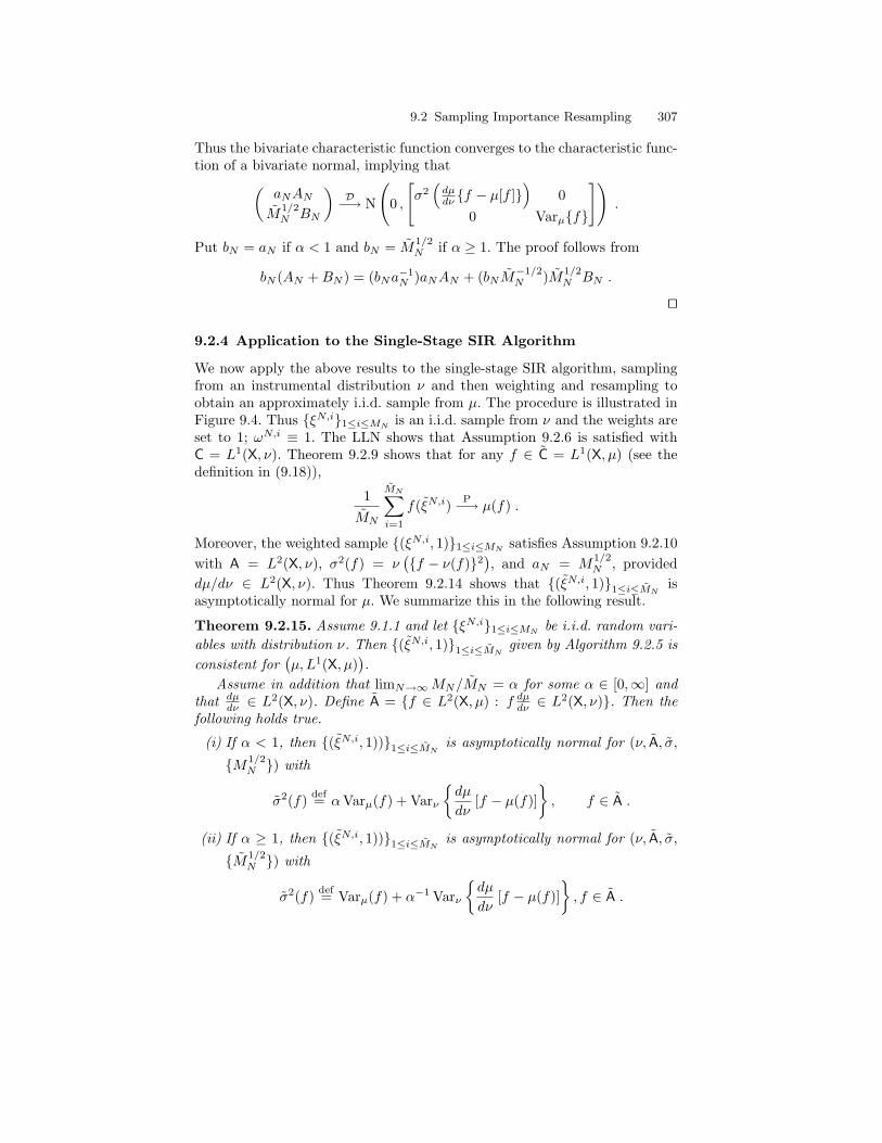
9.2 Sampling Importance Resampling 307

Thus the bivariate characteristic function converges to the characteristic func-tion of a bivariate normal, implying that(

aNAN

M1/2N BN

)D−→ N

(0 ,

[σ2(dµdν f − µ[f ]

)0

0 Varµf

]).

Put bN = aN if α < 1 and bN = M1/2N if α ≥ 1. The proof follows from

bN (AN +BN ) = (bNa−1N )aNAN + (bNM

−1/2N )M1/2

N BN .

ut

9.2.4 Application to the Single-Stage SIR Algorithm

We now apply the above results to the single-stage SIR algorithm, samplingfrom an instrumental distribution ν and then weighting and resampling toobtain an approximately i.i.d. sample from µ. The procedure is illustrated inFigure 9.4. Thus ξN,i1≤i≤MN

is an i.i.d. sample from ν and the weights areset to 1; ωN,i ≡ 1. The LLN shows that Assumption 9.2.6 is satisfied withC = L1(X, ν). Theorem 9.2.9 shows that for any f ∈ C = L1(X, µ) (see thedefinition in (9.18)),

1MN

MN∑i=1

f(ξN,i) P−→ µ(f) .

Moreover, the weighted sample (ξN,i, 1)1≤i≤MNsatisfies Assumption 9.2.10

with A = L2(X, ν), σ2(f) = ν(f − ν(f)2

), and aN = M

1/2N , provided

dµ/dν ∈ L2(X, ν). Thus Theorem 9.2.14 shows that (ξN,i, 1)1≤i≤MNis

asymptotically normal for µ. We summarize this in the following result.

Theorem 9.2.15. Assume 9.1.1 and let ξN,i1≤i≤MNbe i.i.d. random vari-

ables with distribution ν. Then (ξN,i, 1)1≤i≤MNgiven by Algorithm 9.2.5 is

consistent for(µ,L1(X, µ)

).

Assume in addition that limN→∞MN/MN = α for some α ∈ [0,∞] andthat dµ

dν ∈ L2(X, ν). Define A = f ∈ L2(X, µ) : f dµdν ∈ L

2(X, ν). Then thefollowing holds true.

(i) If α < 1, then (ξN,i, 1))1≤i≤MNis asymptotically normal for (ν, A, σ,

M1/2N ) with

σ2(f) def= αVarµ(f) + Varν

dµ

dν[f − µ(f)]

, f ∈ A .

(ii) If α ≥ 1, then (ξN,i, 1))1≤i≤MNis asymptotically normal for (ν, A, σ,

M1/2N ) with

σ2(f) def= Varµ(f) + α−1 Varν

dµ

dν[f − µ(f)]

, f ∈ A .

308 9 Analysis of SMC Methods

! !" "#$ $% % &' ( () ) * *+ , ,- ..// 0 00 0112 23 4567 8 89

:;<= >?@A

B B B B B B B B B B B B B B B B BC C C C C C C C C C C C C C C C C

D D D D D D D D D D D D D D D D D DE E E E E E E E E E E E E E E E E E

Instrumental distribution

Target distribution

F FG G

ν

dµdν

(ξN,MN )dµdν

(ξN,1)

ξN,1 ξN,MN

µ

ξN,1 ξN,MN

µ

Fig. 9.4. The single-stage SIR algorithm.

Without loss of generality, we may assume here that MN = N . To obtaina rate

√N asymptotically normal sample for the target distribution µ, the

cardinality MN of the instrumental sample should grow at least as fast as N ,limN→∞MN/N > 0. If limN→∞MN/N =∞, then

√N [µSIR

ν,N (f)− µ(f)] D−→ N(0,Varµ(f)) ,

that is, the SIR estimator and the plain Monte Carlo estimator µMCN (f)

of µ(f) (the estimator of µ(f) obtained by computing the sample averageN−1

∑Ni=1 f(ξi) with ξi being an i.i.d. sample from the target distribution

µ) have the same limiting Gaussian distribution. In practice, this means thatlarge values for the instrumental sample should be used when one is askingfor a sample that behaves as an i.i.d. sample from µ.

We conclude this section with some elementary deviations inequalities.These inequalities are non-asymptotic and allow evaluating the performanceof the SIR estimator for finite sample sizes.

Theorem 9.2.16. Assume 9.1.1 and let ξN,i1≤i≤MNbe i.i.d. random vari-

ables with distribution ν. Then for any t > 0, f ∈ Fb (X), a ∈ (0, 1), andN ≥ 0,

9.2 Sampling Importance Resampling 309

P

[∣∣∣∣∣M−1N

MN∑i=1

f(ξN,i)− µ(f)

∣∣∣∣∣ ≥ t]

≤ 2 exp[−2MNa

2t2/

osc2(f)]

+ 4 exp[−8MN (1− a)2t2

/9 osc2(f) ‖dµ/dν‖2ν,∞

].

Proof. Decompose M−1N

∑MN

i=1 f(ξN,i)−µ(f) as a sum AN +BN of the twoterms

AN (f) = M−1N

MN∑i=1

f(ξN,i)− E[f(ξN,i) | ξN,1, . . . , ξN,MN ] ,

BN (f) = M−1N

MN∑i=1

E[f(ξN,i) | ξN,1, . . . , ξN,MN ]− µ(f)

=∑MN

i=1dµdν (ξN,i)f(ξN,i)∑MN

i=1dµdν (ξN,i)

−ν(dµdν f

)ν(dµdν

) .

Hoeffding’s inequality implies that

P(|AN (f)| ≥ at

∣∣ ξN,1, . . . , ξN,MN)≤ 2 exp

[−2MNa

2t2/

osc2(f)].

The result also holds unconditionally by taking the expectation of the left-hand side. For P(|BN (f)| ≥ (1−a)t), use the bound (9.12) of Theorem 9.1.10.

ut

Example 9.2.17 (Importance Sampling with Cauchy and GaussianVariables, Continued). In this continuation of Example 9.1.3, the targetdistribution µ is standard Gaussian and the instrumental distribution ν isstandard Cauchy. In this case dµ/dν is bounded by some finite M , so that

ν

[f2

(dµ

dν

)2]≤M ν

(f2 dµ

dν

)≤M µ(f2) .

Hence Theorem 9.2.15 applies to functions f that are square integrable withrespect to the standard Gaussian distribution. This condition is also requiredto establish asymptotic normality of the importance sampling estimator. Weset N =1,000 and investigate the impact of the size M of the instrumentalsample on the accuracy of the SIR estimator for f(x) = exp(−x). Figure 9.5displays the box-and-whisker plot obtained from 500 independent Monte Carloreplications of the IS and SIR estimators of µ(f), for instrumental samplesizes M =100, 1,000, 10,000, and 100,000. As expected, the fluctuations ofthe SIR estimate decrease as the ratio M/N increases. Not surprisingly, when

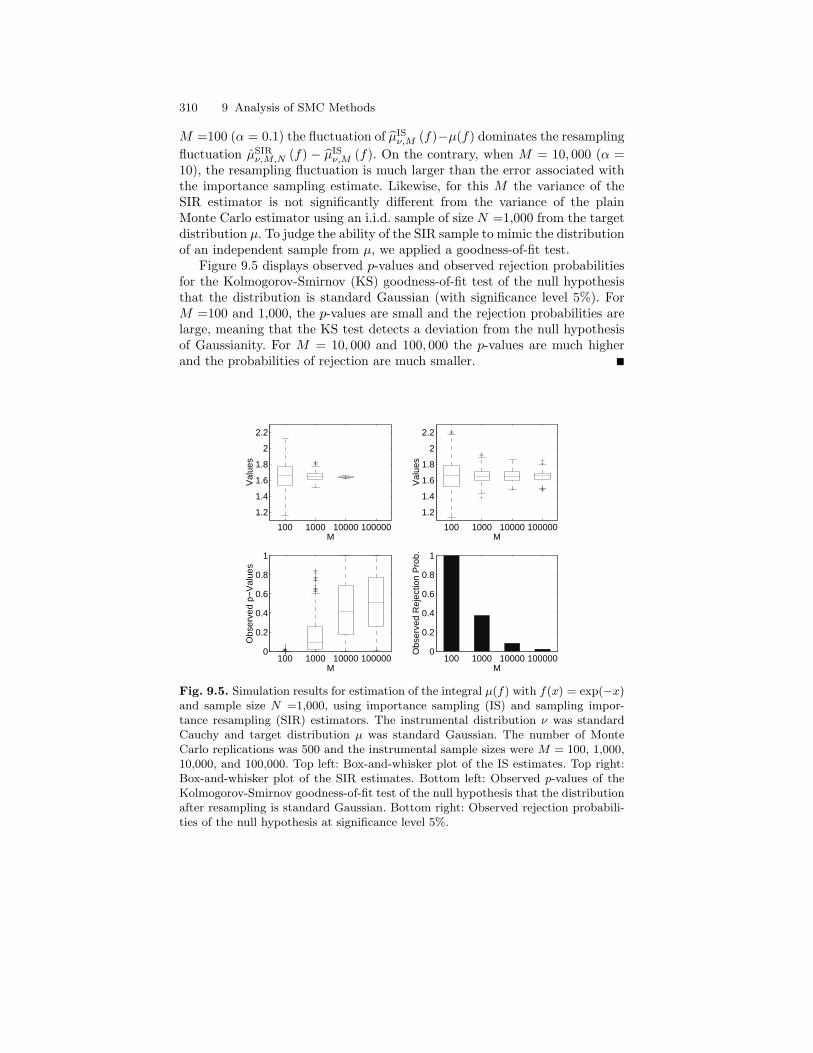
310 9 Analysis of SMC Methods

M =100 (α = 0.1) the fluctuation of µISν,M (f)−µ(f) dominates the resampling

fluctuation µSIRν,M,N (f) − µIS

ν,M (f). On the contrary, when M = 10, 000 (α =10), the resampling fluctuation is much larger than the error associated withthe importance sampling estimate. Likewise, for this M the variance of theSIR estimator is not significantly different from the variance of the plainMonte Carlo estimator using an i.i.d. sample of size N =1,000 from the targetdistribution µ. To judge the ability of the SIR sample to mimic the distributionof an independent sample from µ, we applied a goodness-of-fit test.

Figure 9.5 displays observed p-values and observed rejection probabilitiesfor the Kolmogorov-Smirnov (KS) goodness-of-fit test of the null hypothesisthat the distribution is standard Gaussian (with significance level 5%). ForM =100 and 1,000, the p-values are small and the rejection probabilities arelarge, meaning that the KS test detects a deviation from the null hypothesisof Gaussianity. For M = 10, 000 and 100, 000 the p-values are much higherand the probabilities of rejection are much smaller.

100 1000 10000 100000

1.2

1.4

1.6

1.8

2

2.2

Val

ues

M100 1000 10000 100000

1.2

1.4

1.6

1.8

2

2.2

Val

ues

M

100 1000 10000 1000000

0.2

0.4

0.6

0.8

1

Obs

erve

d p−

Val

ues

M100 1000 10000 100000

0

0.2

0.4

0.6

0.8

1

M

Obs

erve

d R

ejec

tion

Pro

b.

Fig. 9.5. Simulation results for estimation of the integral µ(f) with f(x) = exp(−x)and sample size N =1,000, using importance sampling (IS) and sampling impor-tance resampling (SIR) estimators. The instrumental distribution ν was standardCauchy and target distribution µ was standard Gaussian. The number of MonteCarlo replications was 500 and the instrumental sample sizes were M = 100, 1,000,10,000, and 100,000. Top left: Box-and-whisker plot of the IS estimates. Top right:Box-and-whisker plot of the SIR estimates. Bottom left: Observed p-values of theKolmogorov-Smirnov goodness-of-fit test of the null hypothesis that the distributionafter resampling is standard Gaussian. Bottom right: Observed rejection probabili-ties of the null hypothesis at significance level 5%.

9.3 Single-Step Analysis of SMC Methods 311

9.3 Single-Step Analysis of SMC Methods

We now carry the analysis one step forward to encompass elementary stepsof (some of) the sequential Monte Carlo methods discussed in the previouschapters. To do that, we need to consider transformations of the weightedsample that are more sophisticated than weighting and sampling. As outlinedin the previous chapter, many different actions might be considered, and it isout of the scope of this chapter to investigate all possible variants. We focus inthe following on the SISR approach (Algorithm 7.3.4) and on the variant thatwe called i.i.d. sampling (Algorithm 8.1.1). As discussed in Section 8.1.1, eachiteration of both of these algorithms is composed of two simple procedures—selection and mutation—which we consider separately below.

9.3.1 Mutation Step

To study SISR algorithms, we need first to show that when moving the parti-cles using a Markov transition kernel and then assigning them appropriatelydefined importance weights, we transform a weighted sample consistent (orasymptotically normal) for one distribution into a weighted sample consistent(or asymptotically normal) for another appropriately defined distribution. Asbefore, we let ν be a probability measure on (X,X ), L be a finite transitionkernel on (X,X ), and R be a probability kernel on (X,X ). Define the proba-bility measure µ on (X,X ) by

µ(A) =

∫Xν(dx)L(x,A)∫

Xν(dx)L(x,X)

. (9.27)

We then wish to construct a sample consistent for µ, given a weighted sample(ξN,i, 1)1≤i≤MN

from ν. To do so, we move the particles using R as aninstrumental kernel and then assign them suitable importance weights. Beforewriting down the algorithm, we introduce some assumptions.

Assumption 9.3.1. νL(X) =∫Xν(dx)L(x,X) is positive and finite.

Assumption 9.3.2. (ξN,i, 1)1≤i≤MNis consistent for (ν,C), where C is a

proper set. In addition, the function x 7→ L(x,X) belongs to C.

Assumption 9.3.3. For any x ∈ X, L(x, ·) is absolutely continuous with re-spect to R(x, ·) and there exists a (strictly) positive version of dL(x, ·)/dR(x, ·).

Now let αN be a sequence of integers and put MN = αNMN . Considerthe following algorithm.

Algorithm 9.3.4 (Mutation). Draw ξN,1, . . . , ξN,MN conditionally indepen-dently given FN = GN∨ σ(ξN,1, . . . , ξN,MN ) with distribution

P(ξN,j ∈ A | FN ) = R(ξN,i, A)

312 9 Analysis of SMC Methods

for i = 1, . . . ,MN , j = αN (i− 1) + 1, . . . , αN i, and A ∈ X , and assign ξN,j theweight

ωN,j =dL(ξN,i, ·)dR(ξN,i, ·)

(ξN,j).

Thus each particle gives birth to αN offspring. In many cases, we setαN = 1; then each particle is propagated forward only once. Increasing thenumber αN of offspring increases the particle diversity before the resamplingstep and is thus a practical means for contending particle degeneracy. This ofcourse increases the computational complexity of the algorithm.

Theorem 9.3.5. Assume 9.3.1, 9.3.2 and 9.3.3, and define

Cdef= f ∈ L1(X, µ) : x 7→ L(x, |f |) ∈ C , (9.28)

where µ is given by (9.27). Then C is a proper set and (ξN,i, ωN,i)1≤i≤MN

defined by Algorithm 9.3.4 is consistent for (µ, C).

Proof. Checking that C is proper is straightforward, so we turn to the consis-tency. We prove this by showing that for any f ∈ C,

1MN

MN∑j=1

ωN,jf(ξN,j) P−→ νL(f) . (9.29)

Under the assumptions made, the function x 7→ L(x,X) belongs to C, implyingthat the constant function 1 belongs to C; hence M−1

N

∑MN

j=1 ωN,j converges to

νL(X) in probability. Then for any f ∈ C, the ratio of the two sample meansconsidered tends to νL(f)/νL(X) = µ(f) in probability. This is consistency.

To prove (9.29), pick f in C and note that E[ωN,jf(ξN,j) | FN ] = L(ξN,i, f)for j and i as in Algorithm 9.3.4. Hence

M−1N

MN∑j=1

E[ωN,jf(ξN,j) | FN ] = M−1N

MN∑i=1

L(ξN,i, f) P−→ νL(f) ,

so that it is sufficient to show that

M−1N

MN∑j=1

ωN,jf(ξN,j)− M−1N

MN∑j=1

E[ωN,jf(ξN,j) | FN ] P−→ 0 . (9.30)

For that purpose, we put VN,j = M−1N ωN,jf(ξN,j) and appeal to Propo-

sition 9.5.7; we need to check its conditions (i)–(iii). The triangular arrayVN,j1≤j≤MN

is conditionally independent given FN; this is condition (i).Next, just as above,

9.3 Single-Step Analysis of SMC Methods 313

MN∑j=1

E[|VN,j | | FN ] = M−1N

MN∑i=1

L(ξN,i, |f |) P−→ νL(|f |) ,

showing condition (ii). We finally need to show that for any positive C,

AN =MN∑j=1

E[|VN,j |1|VN,j |≥C | FN ] P−→ 0 .

Put h(x, x′) = dL(x,·)dR(x,·) (x′)|f |(x′). For any positive C, we then have∫

R(x, dx′)h(x, x′)1h(x,x′)≥C ≤∫R(x, dx′)h(x, x′) = L(x, |f |) .

Because the function x 7→ L(x, |f |) ∈ C and the set C is proper, this showsthat the left-hand side of the above display is in C. Hence for large enough N ,

AN ≤M−1N

MN∑i=1

∫R(ξN,i, dx′)h(ξN,i, x′)1h(ξN,i,x′)≥C

P−→∫∫

ν(dx)R(x, dx′)h(x, x′)1h(x,x′)≥C .

The right-hand side of this inequality is bounded by νL(|f |) <∞ (cf. above),so that, by dominated convergence, the right-hand side can be made arbitrarilysmall by letting C → ∞. This shows that AN tends to zero in probability,which is condition (iii). Thus Proposition 9.5.7 applies, (9.30) holds, and theproof is complete. ut

To establish asymptotic normality of the estimators, we must strengthenAssumption 9.3.2 as follows.

Assumption 9.3.6. The weighted sample (ξN,i, 1)1≤i≤MNis asymptoti-

cally normal for (ν,A, σ, M1/2N ), where A is a proper set and σ is a non-

negative function on A.

Theorem 9.3.7. Assume 9.3.1, 9.3.2, 9.3.3, and 9.3.6, and that αN has alimit α, possibly infinite. Define

Adef=f ∈ L2(X, µ) : x 7→ L(x, f) ∈ A and

x 7→∫

X

R(x, dx′)[dL(x, ·)dR(x, ·)

(x′)f(x′)]2

∈ C

. (9.31)

Then A is a proper set and (ξN,i, ωN,i)1≤i≤MNgiven by Algorithm 9.3.4 is

asymptotically normal for (µ, A, σ, M1/2N ) with

314 9 Analysis of SMC Methods

σ2(f) def=σ2 L[f − µ(f)]+ α−1η2[f − µ(f)]

[νL(X)]2, f ∈ A , (9.32)

and η2 defined by

η2(f) def=∫∫

ν(dx)R(x, dx′)[dL(x, ·)dR(x, ·)

(x′)f(x′)]2

−∫ν(dx) [L(x, f)]2 .

(9.33)

Proof. First we note that by definition, α is necessarily at least 1. Checkingthat A is proper is straightforward, so we turn to the asymptotic normality.Pick f ∈ A and assume, without loss of generality, that µ(f) = 0. Write

MN∑i=1

ωN,i∑MN

j=1 ωN,j

f(ξN,i) =MN∑MN

j=1 ωN,j

(AN +BN ) ,

with

AN = M−1N

MN∑i=1

E[ωN,if(ξN,i) | FN ] = M−1N

MN∑i=1

L(ξN,i, f) ,

BN = M−1N

MN∑i=1

ωN,if(ξN,i)− E[ωN,if(ξN,i) | FN ] .

Because MN/∑MN

i=1 ωN,i converges to 1/νL(X) in probability (cf. the proof of

Theorem 9.3.5), the conclusion of the theorem follows from Slutsky’s theoremif we prove that M1/2

N (AN+BN ) converges weakly to N(0, σ2(Lf)+α−1η2(f)).In order to do that, we first note that as the function x 7→ L(x, f) belongs

to A and (ξN,i, 1)1≤i≤MNis asymptotically normal for (ν,A, σ, M1/2

N ),

M1/2N AN

D−→ N(0, σ2(Lf)) .

Next we prove that for any real u,

E[

exp(iuM1/2N BN )

∣∣∣ FN] P−→ exp[−(u2/2)η2(f)

].

For that purpose, we use Proposition 9.5.12, and we thus need to checkits conditions (i)–(iii). Set VN,i = M

−1/2N ωN,if(ξN,i). The triangular array

VN,i1≤i≤MNis conditionally independent given FN [condition (i)]. More-

over, the function x 7→∫R(x, dx′)h2(x, x′) with h(x, x′) = dL(x,·)

dR(x,·) (x′)f(x′)belongs to C. Therefore

MN∑i=1

E[V 2N,i | FN ] P−→

∫∫ν(dx)R(x, dx′)h2(x, x′) ,

9.3 Single-Step Analysis of SMC Methods 315

MN∑i=1

(E[VN,i | FN ])2 P−→∫ν(dx)

[∫R(x, dx′)h(x, x′)

]2

.

These displays imply that condition (ii) holds.It remains to verify (iii), the Lindeberg condition. For any positive C, the

inequality∫X

R(x, dx′)h2(x, x′)1|h(x,x′)|≥C ≤∫

X

R(x, dx′)h2(x, x′)

shows that the function x 7→∫XR(x, dx′)h2(x, x′)1|h(x,x′)|≥C belongs to C.

This yields

M−1N

MN∑i=1

∫R(ξN,i, dx′)h2(ξN,i, x′)1h(ξN,i,x′)≥C

P−→∫∫

ν(dx)R(x, dx′)h2(x, x′)1h(x,x′)≥C .

Because∫∫

ν(dx)R(x, dx′)h2(x′) <∞, the right-hand side of this display canbe made arbitrarily small by letting C →∞. Therefore

MN∑i=1

E[V 2N,i1|VN,i|≥ε | F

N ] P−→ 0 ,

and this is condition (iii).Thus Proposition 9.5.12 applies, and just as in the proof of Theorem 9.2.14

it follows that (M

1/2N AN

M1/2N BN

)D−→ N

(0 ,[σ2(Lf) 0

0 η2(f)

]).

The proof is now concluded upon writing M1/2N (AN + BN ) = M

1/2N AN +

α−1/2N M

1/2N BN . ut

9.3.2 Description of Algorithms

It is now time to combine the mutation step and the resampling step. This canbe done in two different orders, mutation first or selection first, leading to twodifferent algorithms that we call mutation/selection and selection/mutation,respectively. In the mutation/selection algorithm, we first apply the muta-tion algorithm, 9.3.4, to obtain a weighted sample (ξN,i, ωN,i)1≤i≤MN

, andthen resample according to the importance weights. The selection/mutationalgorithm on the other hand is based on a particular decomposition of µ,namely

316 9 Analysis of SMC Methods

µ(A) =∫ν(dx)L(x,A)νL(X)

=∫µ(dx)

L(x,A)L(x,X)

, (9.34)

where

µ(A) def=

∫Aν(dx)L(x,X)νL(X)

, A ∈ X . (9.35)

From a sample (ξN,i, ωN,i)1≤i≤MN, we compute importance weights as

L(ξN,i,X), resample, and finally mutate the resampled system using theMarkov kernel (x,A) 7→ L(x,A)/L(x,X). We now describe the algorithmsformally.

Let αN be a sequence of integers and set MN = αNMN .

Algorithm 9.3.8 (Mutation/Selection).

Mutation: Draw ξN,1, . . . , ξN,MN conditionally independently given FN = GN∨σ(ξN,1, . . . , ξN,MN ), with distribution P(ξN,j ∈ · | FN ) = R(ξN,i, ·) for i =1, . . . ,MN and j = αN (i− 1) + 1, . . . , αN i. Assign ξN,j the weight ωN,j =dL(ξN,i,·)dR(ξN,i,·) (ξN,j).

Sampling: Draw MN random variables IN,1, . . . , IN,MN conditionally indepen-

dently given FN = FN ∨ σ(ξN,1, . . . , ξN,MN ), with the probability of out-

come j, 1 ≤ j ≤ MN , being proportional to ωN,j . Set ξN,i = ξN,IN,i

fori = 1, . . . ,MN .

To avoid notational explosion, it is assumed here that the sample size afterthe resampling stage is identical to the size of the initial sample. Extensionsto general sample sizes are straightforward. The algorithm is illustrated inFigure 9.6.

For the selection/mutation algorithm, we have to strengthen the assump-tion on the transition kernel L.

Assumption 9.3.9. For any x ∈ X, L(x,X) > 0.

Algorithm 9.3.10 (Selection/Mutation).

Selection: Draw random variables IN,1, . . . , IN,MN conditionally independentlygiven FN = GN ∨ σ(ξN,1, . . . , ξN,MN ), with the probability of outcome

j, 1 ≤ j ≤ MN , being proportional to L(ξN,j ,X). Set ξN,i = ξN,IN,i

fori = 1, . . . ,MN .

Mutation: Draw ξN,1, . . . , ξN,MN conditionally independently given FN = FN∨σ(IN,1, . . . , IN,MN ), with distribution P(ξN,i ∈ · | FN ) = L(ξN,i,·)

L(ξN,i,X).

The algorithm is illustrated in Figure 9.7. As described above, the selec-tion/mutation algorithm requires evaluation of, for any x ∈ X, the normal-izing constant L(x,X), and then sampling from the Markov transition kernelL(x, ·)/L(x,X). As emphasized in Chapter 7, these steps are not always easyto carry out. In this sense, this algorithm is in general less widely applicable

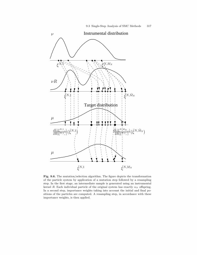
9.3 Single-Step Analysis of SMC Methods 317

! ! "#

$%&'

()*+

,-./ 012 23

4 45 5

67

8 89

:;

<=

>?

@A

BC

D DE E

FG

HI JK LMNO PQ

R RS S

T T T T T T T T T T T T T T T T TU U U U U U U U U U U U U U U U U

Instrumental distribution

Target distribution

V VW

ν

νR

ξN,1 ξN,MN

ξN,1 ξN,MN

ξN,1 ξN,MN

µ

dL(ξN,1,·)dR(ξN,1,·)(ξ

N,1) dL(ξN,MN ,·)dR(ξN,1,·) (ξN,MN)

µ

Fig. 9.6. The mutation/selection algorithm. The figure depicts the transformationof the particle system by application of a mutation step followed by a resamplingstep. In the first stage, an intermediate sample is generated using an instrumentalkernel R. Each individual particle of the original system has exactly αN offspring.In a second step, importance weights taking into account the initial and final po-sitions of the particles are computed. A resampling step, in accordance with theseimportance weights, is then applied.

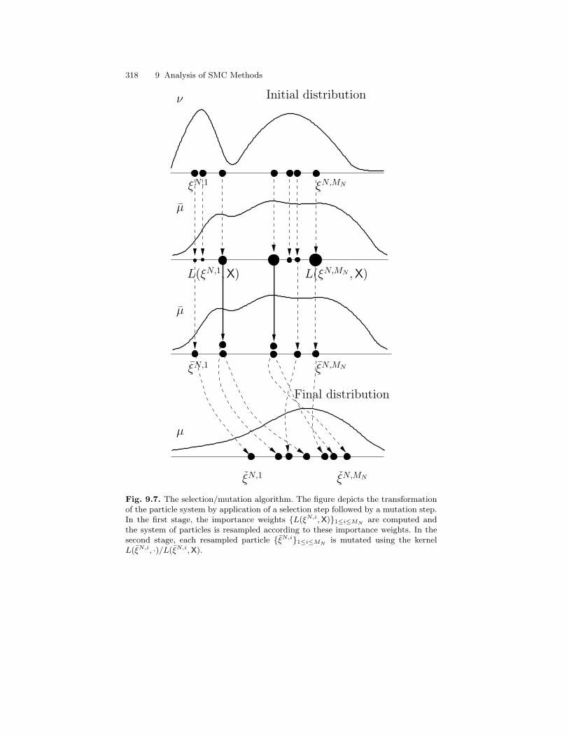
318 9 Analysis of SMC Methods

ξN,MNξN,1

ν

ξN,1 ξN,MN

µ

Initial distribution

µ

µ

L(ξN,1, X) L(ξN,MN , X)

Final distribution

ξN,1 ξN,MN

Fig. 9.7. The selection/mutation algorithm. The figure depicts the transformationof the particle system by application of a selection step followed by a mutation step.In the first stage, the importance weights L(ξN,i,X)1≤i≤MN are computed andthe system of particles is resampled according to these importance weights. In thesecond stage, each resampled particle ξN,i1≤i≤MN is mutated using the kernelL(ξN,i, ·)/L(ξN,i,X).

9.3 Single-Step Analysis of SMC Methods 319

than mutation/selection. However, it is worthwhile to note that the randomvariables ξN,1, . . . , ξN,MN are conditionally independent given FN and dis-tributed according to the mixture of probability kernels

MN∑i=1

L(ξN,i,X)∑MN

j=1 L(ξN,j ,X)

L(ξN,i, A)L(ξN,i,X)

.

As pointed out in Section 8.1.4, it is possible to draw from this distributionwithout having to follow the selection/mutation steps.

9.3.3 Analysis of the Mutation/Selection Algorithm

Using the tools derived above we establish the consistency and asymptoticnormality of the mutation/selection algorithm, 9.3.8. A direct application ofTheorems 9.3.5 and 9.2.9 yields the following result.

Theorem 9.3.11. Assume 9.3.1, 9.3.2, and 9.3.3, and define

Cdef= f ∈ L1(X, µ) : x 7→ L(x, |f |) ∈ C . (9.36)

where µ is given by (9.27). Then C is a proper set and

(i) (ξN,i, ωN,i)1≤i≤MNgiven by Algorithm 9.3.8 is consistent for (µ, C);

(ii) (ξN,i, 1)1≤i≤MNgiven by Algorithm 9.3.8 is consistent for (µ, C).

Moreover, Theorems 9.3.7 and 9.2.14 imply the following.

Theorem 9.3.12. Assume 9.3.1, 9.3.2, 9.3.3, and 9.3.6, and that αN hasa limit, possibly infinite. Define

Adef=f ∈ L2(X, µ) : x 7→ L(x, |f |) ∈ A and

x 7→∫R(x, dx′)

[dL(x, ·)dR(x, ·)

(x′)f(x′)]2

∈ C

.

Then A is a proper set and

(i) (ξN,i, ωN,i)1≤i≤MNgiven by Algorithm 9.3.8 is asymptotically normal

for (µ, A, σ, M1/2N ) with

σ2(f) def=σ2L[f − µ(f)]+ α−1η2[f − µ(f)]

[νL(X)]2, f ∈ A ,

and η2 being defined in (9.33);(ii) (ξN,i, 1)1≤i≤MN

given by Algorithm 9.3.8 is asymptotically normal for(µ, A, σ, M1/2

N ) with σ2(f) = Varµ(f) + σ2(f) for f ∈ A.

320 9 Analysis of SMC Methods

9.3.4 Analysis of the Selection/Mutation Algorithm

We now analyze the selection/mutation algorithm, 9.3.10.

Theorem 9.3.13. Assume 9.3.2 and 9.3.9. Then

(i) (ξN,i, L(ξN,i,X))1≤i≤MNgiven by Algorithm 9.3.10 is consistent for

(µ, C), where µ is defined in (9.35) and

Cdef= f ∈ L1(X, µ) : x 7→ |f(x)|L(x,X) ∈ C ;

(ii) (ξN,i, 1)1≤i≤MNgiven by Algorithm 9.3.10 is consistent for (µ, C),

where

C = f ∈ L1(X, µ) : x 7→ L(x, |f |) ∈ C .

Proof. By construction, µ is absolutely continuous with respect to ν and

dµ

dν(x) =

L(x,X)νL(X)

, x ∈ X . (9.37)

The first assertion follows from Theorem 9.2.7. Theorem 9.2.9 shows that theweighted sample (ξN,i, 1)1≤i≤MN

is consistent for (µ, C). Assertion (ii) thenfollows from the representation (9.34) of µ and Theorem 9.3.5. ut

We may similarly formulate conditions under which the selection/mutationscheme transforms an asymptotically normal sample from the distribution νinto an asymptotically normal sample from µ.

Assumption 9.3.14. (ξN,i, 1)1≤i≤MNis asymptotically normal for (ν,A,

σ, M1/2N ), where A is a proper set and σ is a non-negative function on A.

In addition the function x 7→ L(x,X) belongs to A.

Theorem 9.2.11, Theorem 9.2.14, and Theorem 9.3.7 lead to the followingresult.

Theorem 9.3.15. Assume 9.3.2, 9.3.9, and 9.3.14. Then

(i) (ξN,i, L(ξN,i,X))1≤i≤MNgiven by Algorithm 9.3.10 is asymptotically

normal for (µ, A, σ, M1/2N ), where µ is defined in (9.35),

A = f ∈ L2(X, µ) : x 7→ |f(x)|L(x,X) ∈ A

and

σ2(f) =σ2 L(·,X)[f − µ(f)]

[νL(X)]2, f ∈ A ;

(ii)

(ξN,i, 1)

1≤i≤MNgiven by Algorithm 9.3.10 is asymptotically normal

for (µ, A, σ, M1/2N ), where

A = f ∈ L2(X, µ) : x 7→ L(x, |f |) ∈ A and x 7→ L(x, f2) ∈ C

and

σ2(f) = Varµ(f) +σ2 L[f − µ(f)]

[νL(X)]2, f ∈ A .

9.4 Sequential Monte Carlo Methods 321

9.4 Sequential Monte Carlo Methods

We are now ready to evaluate the performance of repeated applications of thebasic procedures studied in the previous section. We begin with the muta-tion/selection or SISR variant.

9.4.1 SISR

Sequential importance sampling with resampling amounts to successively ap-plying the mutation/selection procedure in order to construct a sample ap-proximating the marginal filtering distribution. In this case, the initial andfinal probability distributions are the marginal filtering distributions φν,k attwo successive time instants. As discussed in Chapter 7, these two distribu-tions are related by (7.8), which we recall here:

φν,0(A) =

∫Aν(dx′) g0(x′)∫

Xν(dx′) g0(x′)

, A ∈ X , (9.38)

φν,k+1(A) =

∫Xφν,k(dx)T u

k (x,A)∫Xφν,k(dx)T u

k (x,X), A ∈ X , k ≥ 0 , (9.39)

T uk (x,A) =

∫A

Q(x, dx′) gk+1(x′) , A ∈ X , (9.40)

where, as usual, Q stands for the transition kernel of the hidden chain and gkfor the likelihood of the current observation, gk(x) = g(x, Yk)1.

The instrumental distributions are defined by a sequence Rkk≥0 of in-strumental transition kernels on (X,X ) and a probability distribution ρ0 on(X,X ). In addition, let αN denote a sequence of positive integers that con-trol the size of the intermediate populations of particles (see below). We re-quire the following assumptions.

Assumption 9.4.1.

(i) ν(g0) > 0.(ii)

∫XQ(x, dx′)gk(x′) > 0 for all x ∈ X and k ≥ 0.

(iii) supx∈X gk(x) <∞ for all k ≥ 0.

Assumption 9.4.2. The instrumental distribution ρ0 for the initial statedominates the filtering distribution φν,0, φν,0 ρ0.

Assumption 9.4.3. For any k ≥ 0 and all x ∈ X, the instrumental kernelRk(x, ·) dominates T u

k (x, ·), T uk (x, ·) Rk(x, ·). In addition, for any x there

exists a version of the Radon-Nikodym derivative dTuk (x,·)

dRk(x,·) that is (strictly)

positive and such that sup(x,x′)∈X×XdTuk (x,·)

dRk(x,·) (x′) <∞.

1Note that in Chapter 7 we defined T uk with a different scale factor—see (7.8).

As mentioned several times, however, this scale factor plays no role in approachesbased on (self-normalized) importance sampling and SIR. For notational simplicity,we thus ignore this scale factor here.

322 9 Analysis of SMC Methods

These conditions are not minimal but are most often satisfied in practice. Thefirst assumption, 9.4.1, implies that for any positive integer k,

0 <∫· · ·∫ν(dx0) g0(x0)

k∏i=1

Q(xi−1, dxi) gi(xi) ≤k∏i=0

supx∈X

gi(x) <∞ ,

so that in particular0 < φν,kT

uk (X) <∞ . (9.41)

The SISR approach under study has already been described in Algo-rithm 7.3.4, which we rephrase below in a more mathematical fashion tounderline the conditioning arguments to be used in the following.

Algorithm 9.4.4 (SISR).

Mutation: Draw ξN,ik+11≤i≤MNconditionally independently given FNk , with dis-

tributionP(ξN,jk+1 ∈ A | F

Nk ) = Rk(ξN,ik , A)

for i = 1, . . . ,MN , j = αN (i − 1) + 1, . . . , αN i and A ∈ X , andcompute the importance weights

ωN,jk+1 = gk+1(ξN,jk+1)dQ(ξN,ik , ·)dRk(ξN,ik , ·)

(ξN,jk+1)

for j and i as above.Selection: Draw IN,1k+1, . . . , I

N,MN

k+1 conditionally independently given FNk = FNk ∨σ(ξN,1k+1, . . . , ξ

N,MN

k+1 ), with distribution

P(IN,ik+1 = j | FNk ) =ωN,jk+1∑MN

j=1 ωN,jk+1

,

and set ξN,ik+1 = ξN,IN,ik+1k+1 and FNk+1 = FNk ∨ σ(ξN,1k+1, . . . , ξ

N,MN

k+1 ).

Two choices, among many others, of the instrumental kernel are the fol-lowing.

Prior kernel: Rk = Q. For any (x, x′) ∈ X × X, [dT uk (x, ·)/dQ(x, ·)](x′) =

gk+1(x′), showing that the importance weights ωN,jk+1 = gk+1(ξN,jk+1) only de-pend on the mutated particle positions. Provided Assumption 9.4.1 holdstrue, so does Assumption 9.4.3 as soon as gk+1(x) > 0 for all x ∈ X. Notethat for the prior kernel, (ξN,ik+1, 1)1≤i≤MN

is a sample approximatingthe marginal predictive distribution φk+1|k = φkQ.

Optimal kernel: Rk = Tk, defined by

Tk(x,A) =T uk (x,A)T uk (x,X)

.

9.4 Sequential Monte Carlo Methods 323

For all (x, x′) ∈ X× X, [dT uk (x, ·)/dTk(x, ·)](x′) = T u

k (x,X), which impliesthat the importance weights ωN,jk+1 = T u

k (ξN,i,X), with j and i as above,only depend on the current particle positions. Provided Assumption 9.4.1holds true, so does Assumption 9.4.3 because, for all (x, x′) ∈ X × X,[dT u

k (x, ·)/dTk(x, ·)] > 0 and

sup(x,x′)∈X×X

dT uk (x, ·)

dTk(x, ·)(x′) = sup

x∈X

∫X

Q(x, dx′) gk+1(x′) ≤ supx∈X

gk+1(x) <∞ .

For all other instrumental kernels, the importance weights depend on theinitial and final positions of the particles.

Theorem 9.4.5. Assume 9.4.1, 9.4.2, and 9.4.3. Then the following holdstrue.

(i) If (ξN,i0 , 1)1≤i≤MNis consistent for (φν,0, L1(X, φν,0)) then for any k >

0, (ξN,ik , 1)1≤i≤MNis consistent for (φν,k, L1(X, φν,k)).

(ii) If in addition (ξN,i0 , 1)1≤i≤MNis asymptotically normal for (φν,0,

L2(X, φν,0), σ0, M1/2N ) then for any k > 0, (ξN,ik , 1)1≤i≤MN

is asymp-totically normal for (φν,k, L2(X, φν,k), σk, M1/2

N ), where the sequenceσk of functions is defined recursively, for f ∈ L2(X, φν,k), by

σ2k+1(f) = Varφν,k+1(f)

+σ2k(T u

k f − φν,k+1(f)) + α−1η2k(f − φν,k+1(f)2)

(φν,kT uk (X))2

with

η2k(f) =

∫∫φν,k(dx)Rk(x, dx′)

dT u

k (x, ·)dRk(x, ·)

(x′)f(x′)2

−∫∫

φν,k(dx)T uk (x, f)2 .

Proof. The proof is by induction over k. Starting with (i), we hence assumethat for some k ≥ 0, (ξN,i, 1)1≤i≤MN

is consistent for (φν,k, L1(X, φν,k)). Toprove that consistency then holds for k + 1 as well, we shall employ Theo-rem 9.3.11 and hence need to verify its underlying assumptions with ν = φν,kand L = T u

k . To start with, Assumption 9.3.1 is (9.41) and Assumption 9.3.3is implied by Assumption 9.4.3. Assumption 9.3.2 follows from the inductionhypothesis plus the bound T u

k (x,X) ≤ ‖gk+1‖∞ < ∞ for all x. Finally, tocheck that consistency applies over L1(X, φν,k+1), we need to verify that forany f ∈ L1(X, φν,k+1) the function x 7→ T u

k (x, |f |) belongs to L1(X, φν,k). Thisis indeed true, as

324 9 Analysis of SMC Methods

(φν,kT uk )(|f |) = (φν,kT u

k )(X)× φν,k+1(|f |).

Assertion (i) now follows from Theorem 9.3.11 and induction.We proceed to part (ii), modify the induction hypothesis accordingly, and

use Theorem 9.3.12 to propagate it from k to k+1. The additional assumptionwe then need to verify is Assumption 9.3.6, which is the induction hypothesis.Finally, we need to check that asymptotic normality applies over L2(X, φν,k+1).Pick f ∈ L2(X, φν,k+1). Then by Jensen’s inequality,

φν,k[(T uk |f |)2

]= φν,k

([Q(gk+1|f |)]2

)≤ φν,kQ(g2

k+1f2)

= (φν,kT uk )(X)φν,k+1(gk+1f

2)≤ (φν,kT u

k )(X) ‖gk+1‖∞ φν,k+1(f2) <∞ ,

saying that T uk (|f |) is in L2(X, φν,k). Similarly

∫X

φν,k(dx)∫

X

Rk(x, dx′)[dT u

k (x, ·)dRk(x, ·)

(x′)f(x′)]2

≤ sup(x,x′)∈X×X

dT uk (x, ·)

dRk(x, ·)(x′) (φν,kT u

k )(X)φν,k+1(f2) <∞ ,

so that the function that φν,k is acting on in the left-hand side belongs toL1(X, φν,k). Assertion (ii) now follows from Theorem 9.3.12 and induction.

ut

9.4.2 I.I.D. Sampling

We now consider successive applications of the selection/mutation procedure.The resulting algorithm, referred to as i.i.d. sampling in Section 8.1.1, is re-called below. Because the mathematical analysis of this algorithm is somewhatsimpler, we consider below two additional types of results: uniform (in time)convergence results under appropriate forgetting conditions (as discussed inSection 4.3) and exponential tail inequalities. Recall that although the empha-sis is here put on filtering estimates, the selection/mutation algorithm mayalso be applied to approximate the predictive distributions, in which case it isknown as the bootstrap filter (Figure 8.1). Hence all results below also applyto the analysis of the predictive estimates produced by the bootstrap filter,with only minor adjustments.

Algorithm 9.4.6 (I.I.D. Sampling).

Selection: Assign to the particle ξN,ik the importance weight

ωN,ik+1 = T uk (ξN,ik ,X) =

∫X

Q(ξN,ik , dx′) gk+1(x′) .

9.4 Sequential Monte Carlo Methods 325

Draw IN,1k+1, . . . , IN,MN

k+1 conditionally independently given FNk , with distribu-tion

P(IN,ik+1 = j | FNk ) =ωN,jk∑MN

j=1 ωN,jk

, i, j = 1, . . . ,MN ,

and set ξN,ik = ξN,IN,ik+1k .

Mutation: Draw ξN,1k+1, . . . , ξN,MN

k+1 conditionally independently given FNk = FNk ∨σ(IN,1k+1, . . . , I

N,MN

k+1 ), with distribution

P(ξN,ik+1 ∈ A | FNk ) =

T uk (ξN,ik , A)

T uk (ξN,ik ,X)

=

∫AQ(ξN,ik , dx′) gk+1(x′)∫

XQ(ξN,ik , dx′) gk+1(x′)

.

9.4.2.1 Consistency and Asymptotic Normality

Theorem 9.4.7. Assume 9.4.1, 9.4.2, and 9.4.3. Then the following holdstrue.

(i) If (ξN,i0 , 1)1≤i≤MNis consistent for (φν,0, L1(X, φν,0)) then for any k >

0, (ξN,ik , 1)1≤i≤MNis consistent for (φν,k, L1(X, φν,k)).

(ii) If (ξN,i0 , 1)1≤i≤MNis asymptotically normal for (φν,0, L2(X, φν,0), σ0,

M1/2N ), then for any k > 0, (ξN,ik , 1)1≤i≤MN

is asymptotically normalfor (φν,k, L2(X, φν,k), σk, M1/2

N ), where the sequence σk of functionsis defined recursively by

σ2k+1(f) = Varφν,k+1(f) +

σ2k T u

k [f − φν,k+1(f)][φν,kT u

k (X)]2, f ∈ L2(X, φν,k+1) .

(9.42)

Proof. Again the proof is by induction. Hence assume that for some k ≥ 0,(ξN,ik , 1)1≤i≤MN

is consistent for (φν,k, L1(X, φν,k)). To carry the inductionhypothesis from k to k + 1, we shall employ Theorem 9.3.13 and thus needto check its underlying assumptions. Assumption 9.3.2 was verified in theproof of Theorem 9.4.5, and (9.3.9) is Assumption 9.4.1(ii). What remains tocheck is that consistency holds over the whole of L1(X, φν,k+1), and for thatwe must verify that for every f in this space, the function T u

k (|f |) belongs toL1(X, φν,k). This was also done in the proof of Theorem 9.4.5. Hence assertion(i) follows from Theorem 9.3.13 and induction.

We proceed to part (ii), modify the induction hypothesis accordingly, anduse Theorem 9.3.15 to propagate it from k to k+1. The additional assumptionwe then need to verify is Assumption 9.3.14, which follows from the inductionhypothesis and the bound T u

k (x,X) ≤ ‖gk+1‖∞. Finally, we establish thatasymptotic normality applies over L2(X, φν,k+1), which amounts to verifyingthat for any f ∈ L2(X, φν,k+1), the function T u

k (|f |) belongs to L2(X, φν,k) andthe function T u

k (f2) belongs to L1(X, φν,k+1). The first of these requirements

326 9 Analysis of SMC Methods

is part of the proof of Theorem 9.4.5, and the proof of the second requirementis entirely analogous. Assertion (ii) now follows from Theorem 9.3.15 andinduction. ut

It is worthwhile to note that the asymptotic variance of the i.i.d. samplingalgorithm is always lower than that of SISR, whatever choice of instrumentalkernel for the latter. This indicates that whenever possible, i.i.d. samplingshould be preferred. By iterating (9.42), one can obtain an analytic expressionfor the asymptotic variance.

Proposition 9.4.8. Assume 9.4.1 and 9.4.3 and that (ξN,i0 , 1)1≤i≤MNis

asymptotically normal for (φν,0, L2(X, φν,0), σ0, M1/2N ). Then for any k ≥ 0

and f ∈ L2(X, φν,k),

σ2k(f) =

k∑l=1

Varφν,lT ul · · ·T u

k−1[f − φν,k(f)][

φν,lT ul · · ·T u

k−1(X)]2

+σ2

0

T u

0 · · ·T uk−1[f − φν,k(f)]

[φν,0T u

0 · · ·T uk−1(X)

]2 ,

where, by convention T ui · · ·T u

j (x,A) is the identity transition kernel δx(A)for i > j.

Proof. The proof is by induction on k. The result holds true for k = 0. Assumenow that the result holds true for some k ≥ 0. We evaluate the right-handside of (9.42) with the claimed formula for σ2

k. Doing this, we first note thatT uk [f−φν,k+1(f)]−φν,kT u

k [f−φν,k+1(f)] = T uk [f−φν,k+1(f)], because φν,kT u

k

equals φν,k+1 up to a multiplicative constant. Thus the right-hand side of(9.42) evaluates to

Varφν,k+1(f) +k∑l=1

Varφν,l T ul · · ·T u

k [f − φν,k+1(f)][φν,lT u

l · · ·T uk−1(X)

]2 [φν,kT uk (X)]2

+σ2

0 T u0 · · ·T u

k [f − φν,k(f)][φν,0T u

0 · · ·T uk−1(X)

]2 [φν,kT uk (X)]2

.

Comparing this with the claimed expression for σ2k+1(f), we see that what

remains to verify is that the denominators of the above ratios equal the squareof φν,lT u

l · · ·T uk (X).

To do that, we observe that the definition of the filtering distribution—seefor instance (3.13)—shows that for any l ≤ k − 1,

9.4 Sequential Monte Carlo Methods 327

φν,k(h) = L−1ν,k

∫· · ·∫ν(dx0) g0(x0)

k∏i=1

Q(xi−1, dxi) gi(xi)h(xk)

= Lν,lL−1ν,k

∫· · ·∫φν,l(dxl)

k∏i=l+1

Q(xi−1, dxi) gi(xi)h(xk)

=φν,lT

ul · · ·T u

k−1f

φν,lT ul · · ·T u

k−1(X).

Setting h = T uk (X) yields [φν,kT u

k (X)]φν,lT ul · · ·T u

k−1(X) = φν,lTul · · ·T u

k (X).The proof now follows by induction. ut

The expression for the asymptotic variance is rather involved, and it is dif-ficult in general to make simple statements on this quantity. There is howevera situation in which some interesting conclusions can be drawn. Consider thefollowing assumption (cf. Lemma 4.3.25).

Assumption 9.4.9. There exist positive constants σ− and σ+ and a proba-bility distribution λ such that 0 < σ−λ(A) ≤ Q(x,A) ≤ σ+λ(A) < ∞ for allx ∈ X and A ∈ X .

Also recall the notation ρdef= 1− σ−/σ+.

Under this condition, it has been shown that the posterior chain is uni-formly geometrically mixing, that is, it forgets its initial condition uniformlyand at a geometric (or exponential) rate. Exponential forgetting allows usto prove that the asymptotic variance of the selection/mutation algorithmremains bounded.

Proposition 9.4.10. Assume 9.4.1, 9.4.3, and 9.4.9. Then for any f ∈Fb (X), it holds that supk≥0 σ

2k(f) <∞, where σ2

k is defined in (9.42).

Proof. Consider the numerators of the ratios of the expression for σk in Propo-sition 9.4.8. Proposition 3.3.2 shows that for any integers l < k,

T ul · · ·T u

k−1(x,A) = βl|k(x)Fl|k · · ·Fk−1|k(x,A) , x ∈ X, A ∈ X ,

where the Fl|k are forward smoothing kernels (see Definition 3.3.1) and βl|kis the backward function (see Definition 3.1.6). Therefore

T ul · · ·T u

k−1f(x)− T ul · · ·T u

k−1(x,X)φν,k(f)

= βl|k(x)[Fl|k · · ·Fk−1|kf(x)− φν,k(f)

]. (9.43)

Next we consider the denominators of the expression for σk. We haveφν,lT

ul · · ·T u

k−1(X) = φν,l(βl|k) =∏kj=l+1 cν,j , where the first equality follows

from the above and the second one from Proposition 3.2.5, and where theconstants cν,j are defined recursively in (3.22). Moreover, by (3.26) Lν,k =∏kj=0 cν,j , and hence

328 9 Analysis of SMC Methods

φν,lTul · · ·T u

k−1(X) =Lν,kLν,l

. (9.44)

Combining (9.43) and (9.44) yields for any integers l ≤ k,

Varφν,lT ul · · ·T u

k−1[f − φν,k(f)][

φν,lT ul · · ·T u

k−1(X)]2

= Varφν,l

(βl|k

Lν,lLν,kFl|k · · ·Fk−1|kf − φν,k(f)

). (9.45)

In order to bound this variance, we first notice that Lemma 4.3.22(ii) showsthat

βl|k(x)Lν,lLν,k

=

∫Q(x, dx′) gl+1(x′)βl+1|k(x′)∫∫

φν,l(dx)Q(x, dx′) gl+1(x′)βl+1|k(x′)≤ σ+

σ−=

11− ρ

.

(9.46)Next, Proposition 3.3.4 shows that φν,k(f) = φν,l|kFl|k · · ·Fk−1|kf , whereφν,l|k is a smoothing distribution. In addition, by Lemma 4.3.22 again, forany probability measures ξ and ξ′ on (X,X ),∥∥ξFl|k · · ·Fk−1|k − ξ′Fl|k · · ·Fk−1|k

∥∥TV≤ ρk−l ‖ξ − ξ′‖TV .

Applying this bound with ξ = δx and ξ′ = φν,l|k shows that

|Fl|k · · ·Fk−1|k(x, f)− φν,l|k(f)| ≤ 2ρk−l ‖f‖∞ .

Finally, combining with (9.45) and (9.46) shows that

Varφν,lT ul · · ·T u

k−1[f − φν,k(f)][

φν,lT ul · · ·T u

k−1(X)]2 ≤ 4(1− ρ)−2ρ2(k−l) ‖f‖2∞ .

This bound together with Proposition 9.4.8 completes the proof. ut

9.4.2.2 Exponential Inequalities

The induction argument previously used for the central limit theorem mayalso be used to derive exponential inequalities for the tail probabilities.

Theorem 9.4.11. Assume 9.4.1 and that there exist some constants a(0) andb(0) such that for any t ≥ 0 and f ∈ Fb (X),

P

[∣∣∣∣∣M−1N

MN∑i=1

f(ξN,i0 )− φν,0(f)

∣∣∣∣∣ ≥ t]≤ a(0) exp

[− 2MN t

2

b(0)2 osc2(f)

]. (9.47)

Then for any k > 0, t > 0 and f ∈ Fb (X),

9.4 Sequential Monte Carlo Methods 329

P

[∣∣∣∣∣M−1N

MN∑i=1

f(ξN,ik )− φν,k(f)

∣∣∣∣∣ ≥ t]≤ a(k) exp

[− 2MN t

2

b(k)2 osc2(f)

], (9.48)

where the constants a(k) and b(k) are defined recursively through

a(k + 1) = 2 (1 + a(k)) ,

b(k + 1) =(3/2) ‖gk+1‖∞ b(k) + φν,kT

uk (X)

φν,kT uk (X)

.

Proof. The proof is by induction; assume that the claim is true for some k ≥ 0.Decompose M−1

N

∑MN

k=1 f(ξN,ik+1)−φν,k+1(f) in two terms ANk+1(f) +BNk+1(f),where

ANk+1(f) = M−1N

MN∑i=1

(f(ξN,ik+1)− E[f(ξN,ik+1) | FNk ])

BNk+1(f) = M−1N

MN∑i=1

E[f(ξN,ik+1) | FNk ]− φν,k+1(f)

=∑MN

k=1 Tuk f(ξN,ik )∑MN

k=1 Tuk (ξN,ik ,X)

− φν,kTuk f

φν,kT uk (X)

.

Proceeding like in Theorem 9.2.16, for any a ∈ (0, 1) and t ≥ 0,

P(|ANk+1(f)| ≥ at) ≤ 2 exp[−2a2t2MN/ osc2(f)

]. (9.49)

We now bound BNk+1(f). First note first for any constant c, BNk+1(f) =BNk+1(f − c). We choose c in such a way that ‖f − c‖∞ = (1/2) osc (f) andset f = f − c. Writing

BNk+1(f) =M−1N

∑Mn

i=1T uk f(ξN,ik )− φν,kT u

k fφν,kT u

k (X)

−∑MN

i=1 Tuk f(ξN,ik )∑MN

i=1 Tuk (ξN,ik ,X)

M−1N

∑MN

i=1 T uk (ξN,ik ,X)− φν,kT u

k (X)φν,kT u

k (X)(9.50)

and using the induction assumption, it holds that for any b ∈ (0, 1),

P[|BNk+1(f)| ≥ (1− a)t

]≤ a(k) exp

−2MN (1− a)2b2t2[φν,kT u

k (X)]2

b2(k) osc2(T uk f)

+ a(k) exp

−2MN (1− a)2(1− b)2t2[φν,kT u

k (X)]2

b2(k)∥∥f∥∥2

∞ osc2(T uk 1)

.

By Lemma 4.3.4, for any (x, x′) ∈ X× X,

330 9 Analysis of SMC Methods

|T uk f(x)− T u

k f(x′)| = |Q(x, gk+1f)−Q(x′, gk+1f)|≤ (1/2) ‖Q(x, ·)−Q(x′, ·)‖TV osc

(gk+1f

)≤ ‖gk+1‖∞ osc (f) ,

and similarly,

|T uk (x,X)− T u

k (x′,X)| = |Q(x, gk+1)−Q(x′, gk+1)| ≤ ‖gk+1‖∞ .

Thus, osc(T uk f)

and osc (T uk 1) are bounded by ‖gk+1‖∞ osc (f) and ‖gk+1‖∞,

respectively. The result follows by choosing b = 2/3 as in the proof of Theo-rem 9.1.10 and then setting a to equate the bounds on ANk+1(f) and BNk+1(f).

ut

The bound is still of Hoeffding type, but at each iteration the constantsa(k) and b(k) increase. Hence, the obtained bound is almost useless in practicefor large k, except when the number of iterations is small or the number ofparticles is large (compared to the iteration index). It would of course bemore appropriate to derive an exponential bound with constants that do notdepend on the iteration index. Such results hold true when Q satisfies thestrong mixing condition.

Theorem 9.4.12. Assume 9.4.1, 9.4.9, and (9.47). Then there exist con-stants a and b such that for any n ≥ 0, t ≥ 0 and f ∈ Fb (X),

P

[∣∣∣∣∣M−1N

MN∑i=1

f(ξN,in )− φν,n(f)

∣∣∣∣∣ ≥ t]≤ a exp

[− 2MN t

2

b2 osc2(f)

].

Proof. Define φNk = M−1N

∑MN

i=1 δξN,ik. The difference φNn (f)− φν,n(f) may be

expressed as the telescoping sum

φNn (f)− φν,n(f) =φN0 T

u0 · · ·T u

n−1f

φN0 Tu0 · · ·T u

n−1(X)− φν,n(f)+

n∑k=1

φNk T

uk · · ·T u

n−1f

φNk Tuk · · ·T u

n−1(X)−

φNk−1Tuk−1 · · ·T u

n−1f

φNk−1Tuk−1 · · ·T u

n−1(X)

, (9.51)

with the convention that T uk · · ·T u

n−1 is the identity mapping when k = n. Weshall show that the tail probabilities of each of the terms on the right-handside of (9.51) are exponentially small. Put

ANn (f) =φN0 T

u0 · · ·T u

n−1f

φN0 Tu0 · · ·T u

n−1(X)− φν,n(f) (9.52)

=∑MN

i=1 β0|n(ξN,i0 )F0|n · · ·Fn−1|nf(ξN,i0 )− φν,n(f)∑MN

i=1 β0|n(ξN,i0 ), (9.53)

9.4 Sequential Monte Carlo Methods 331

where φν,n(f) could also be rewritten as φν,0T u0 · · ·T u

n−1(f) (see Section 3.3.1).Thus by Lemma 4.3.4 and Proposition 4.3.23(i),∥∥F0|n · · ·Fn−1|n(·, f)− φν,n(f)

∥∥∞ ≤ ρ

n osc (f) (9.54)

andosc(F0|n · · ·Fn−1|n(·, f)

)≤ ρn osc (f) . (9.55)

In additionφν,0(β0|n)

osc(β0|n(·)

) ≥ φν,0(β0|n)2∥∥β0|n(·)

∥∥∞≥ σ−

σ+= 1− ρ , (9.56)

where Lemma 4.3.22(ii) was used for the second inequality. Writing

ANn (f) = M−1N

∑MN

i=1 β0|n(ξN,i0 )F0|n · · ·Fn−1|nf(ξN,i0 )− φν,n(f)φν,0(β0|n)

+∑MN

i=1 β0|n(ξN,i0 )F0|n · · ·Fn−1|nf(ξN,i0 )− φν,n(f)∑MN

i=1 β0|n(ξN,i0 )

×

[1−M−1

N

∑MN

i=1 β0|n(ξN,i0 )φν,0(β0|n)

]

we have, using (9.54) and the triangle inequality,

ANn (f) ≤M−1N

∣∣∣∣∣∑MN

i=1 β0|n(ξN,i0 )F0|n · · ·Fn−1|nf(ξN,i0 )− φν,n(f)φν,0(β0|n)

∣∣∣∣∣+ ρn osc (f)M−1

N

∣∣∣∣∣∑MN

i=1 β0|n(ξN,i0 )− φν,0(β0|n)φν,0(β0|n)

∣∣∣∣∣ .Using (9.56) as well as (9.47) twice (for the functions F0|n · · ·Fn−1|nf andβ0|n) shows that for any t ≥ 0,

P[|ANn (f)| ≥ t

]≤ 2a(0) exp

[− MN t

2(1− ρ)2

2b2(0) osc2(f) ρ2n

]. (9.57)

For 1 ≤ k ≤ n, put

∆Nk,n(f) =

φNk Tuk · · ·T u

n−1f

φNk Tuk · · ·T u

n−1(X)−

φNk−1Tuk−1 · · ·T u

n−1f

φNk−1Tuk−1 · · ·T u

n−1(X). (9.58)

Proposition 3.3.2 shows that T uk · · ·T u

n−1(x,A) = βk|n(x)Fk|n · · ·Fn−1|n(x,A).Pick x0 ∈ X. Then

φNk Tuk · · ·T u

n−1f

φNk Tuk · · ·T u

n−1(X)− Fk|n · · ·Fn−1|n(x0) =

βk|n(ξN,ik )ψk|n(ξN,ik )∑MN

i=1 βk|n(ξN,ik ), (9.59)

332 9 Analysis of SMC Methods

where ψk|n(x) = Fk|n · · ·Fk−1|nf(x)− Fk|n · · ·Fk−1|nf(x0). Set

φNk =φNk−1T

uk−1

φNk−1Tuk−1(X)

and µNk|n(A) =

∫AφNk (dx)βk|n(x)∫

XφNk (dx)βk|n(x)

.

Then µNk|n φNk , with Radon-Nikodym derivative

dµNk|n

dφNk(x) =

βk|n(x)

φNk (βk|n).

Using these notations,

φNk−1Tuk−1 · · ·T u

n−1f

φNk−1Tuk−1 · · ·T u

n−1(X)− Fk|n · · ·Fn−1|nf(x0) =

φNk[βk|nFk|n · · ·Fn−1|nf − Fk|n · · ·Fn−1|nf(x0)

]φNk (βk|n)

= µNk|n(ψk|n) . (9.60)

Combining (9.59) and (9.60), we may express ∆Nk,n(f) as

∆Nk,n(f) =

∑MN

i=1

dµNk|n

dφNk(ξN,ik )ψk|n(ξN,ik )∑MN

i=1

dµNk|n

dφNk(ξN,ik )

− µNk|n(ψk|n) .

Because ξN,ik 1≤i≤MNare conditionally i.i.d. given FNk−1 with common

distribution φNk , the first term in the above expression may be seen as an im-portance sampling estimator of µNk|n(ψk|n). By Lemma 4.3.22(ii), the Radon-

Nikodym derivative dµNk|n/dφNk (x) is bounded uniformly in k, N and x as

dµNk|n

dφNk(x) ≤ σ+

σ−=

11− ρ

.

Proceeding as above, the Hoeffding inequality implies that for any t ≥ 0,

P[∣∣∆N

k,n(f)∣∣ ≥ t] ≤ 2 exp

[− MN t

2(1− ρ)2

2 osc2(f) ρ2(n−k)

].

Hence the probability that the sum on the right-hand side of (9.51) is (inabsolute value) at least t is bounded by

2n−1∑k=0

exp[−MN t

2(1− ρ)2b2k2 osc2(f) ρ2k

](9.61)

for any sequence bk0≤k≤n−1 of positive numbers summing to one. To obtaina bound that does not depend on n, take bk = θk(1−θ)/(1−θn) with ρ < θ < 1.This choice proves that (9.61) is bounded by

9.5 Complements 333

a exp[−MN t

2(1− ρ)2(1− θ2)2 osc2(f)

],

where a is a constant that depends only on θ and ρ. ut

9.5 Complements

9.5.1 Weak Limits Theorems for Triangular Array

This section summarizes various basic results on the asymptotics of triangulararrays that are used in the proofs of this chapter.

9.5.1.1 Law of Large Numbers

Throughout this section, MNN≥0 denotes a sequence of integers. All randomvariables are assumed to be defined on a common probability space (Ω,F ,P).

Proposition 9.5.1. Let UN,i1≤i≤MNbe a triangular array of random vari-

ables and let FNN≥0 be a sequence of sub-σ-fields of F . Assume that thefollowing conditions hold true.

(i) The triangular array is conditionally independent given FN and forany N and i = 1, . . . ,MN , E[|UN,i| | FN ] <∞ and E[UN,i | FN ] = 0.

(ii) For some positive ε,

MN∑i=1

E[U2N,i1|UN,i|<ε | F

N ] P−→ 0 , (9.62)

MN∑i=1

E[|UN,i|1|UN,i|≥ε | FN ] P−→ 0 . (9.63)

ThenMN∑i=1

UN,iP−→ 0 .

Proof. Consider the truncated random variable UN,i = UN,i1|UN,i|<ε. Using(9.63) and E[UN,i | FN ] = 0, we find that

MN∑i=1

E[UN,i | FN ] P−→ 0 . (9.64)

By Chebyshev’s inequality, it follows that for any δ > 0,

334 9 Analysis of SMC Methods

AN (δ) = P

(∣∣∣∣∣MN∑i=1

UN,i −MN∑i=1

E[UN,i | FN ]

∣∣∣∣∣ ≥ δ∣∣∣∣∣ FN

)

≤ δ−2 Var

(MN∑i=1

UN,i

∣∣∣∣∣ FN),

and hence (9.62) shows that AN (δ) → 0 in probability. Because AN (δ) isobviously bounded, we also have E[AN (δ)]→ 0, that is,

MN∑i=1

UN,i −MN∑i=1

E[UN,i | FN ] P−→ 0 . (9.65)

Moreover, for any δ > 0,

P

(∣∣∣∣∣MN∑i=1

UN,i −MN∑i=1

UN,i

∣∣∣∣∣ ≥ δ∣∣∣∣∣FN

)≤ P

(MN∑i=1

|UN,i|1|UN,i|≥ε ≥ δ

∣∣∣∣∣FN)

≤ δ−1MN∑i=1

E[|UN,i|1|UN,i|≥ε | FN ] P−→ 0 .

Thus,∑MN

i=1 UN,i−∑MN

i=1 UN,i → 0 in probability. Combining with (9.64) and(9.65), the proof is complete. ut

Definition 9.5.2 (Bounded in Probability). A sequence ZNN≥0 ofrandom variables is said to be bounded in probability if

limC→∞

supN≥0

P(|ZN | ≥ C) = 0.

Often the term tight, or asymptotically tight, is used instead of “bounded inprobability”. We recall without proof the following elementary properties.

Lemma 9.5.3.

1. Let UNN≥0 and U be random variables. If UND−→ U , then UN is

bounded in probability.2. Let UNN≥0 and VNN≥0 be two sequences of random variables. If VN

is bounded in probability and |UN | ≤ |VN | for any N , then UN is boundedin probability.

3. Let UNN≥0 and VNN≥0 be two sequences of random variables. IfUNN≥0 is bounded in probability and VN → 0 in probability, thenUNVN → 0 in probability.

4. Let UNN≥0 be a sequence of random variables and let MNN≥0 bea non-decreasing deterministic sequence diverging to infinity. If UN isbounded in probability, then 1UN≥MN → 0 in probability.

9.5 Complements 335

The following elementary lemma is repeatedly used in the sequel.

Lemma 9.5.4. Let UNN≥0 and VNN≥0 be two sequences of random vari-ables such that VN is bounded in probability. Assume that for any posi-tive η there exists a sequence WN (η)N≥0 of random variables such that

WN (η) P−→ 0 as N →∞ and

|UN | ≤ ηVN +WN (η) .

Then UNP−→ 0.

Proof. For any δ > 0,

P(|UN | ≥ δ) ≤ P[VN ≥ δ/(2η)] + P[WN (η) ≥ δ/2] .

This implies that for any η > 0,

lim supN→∞

P(|UN | ≥ δ) ≤ supN≥0

P[VN ≥ δ/(2η)] .

Because the right-hand side can be made arbitrarily small by letting η → 0,the result follows. ut

Proposition 9.5.5. Let UN,i1≤i≤MNbe a triangular array of random vari-

ables and let FNN≥0 be a sequence of sub-σ-fields of F . Assume that thefollowing conditions hold true.

(i) The triangular array is conditionally independent given FN and forany N and i = 1, . . . ,MN , E[|UN,i| | FN ] <∞ and E[UN,i | FN ] = 0.

(ii) The sequence of random variablesMN∑i=1

E[|UN,i| | FN ]

N≥0

(9.66)

is bounded in probability.(iii) For any positive η,

MN∑i=1

E[|UN,i|1|UN,i|≥η | FN ] P−→ 0 . (9.67)

ThenMN∑i=1

UN,iP−→ 0 .

Proof. We employ Proposition 9.5.1 and then need to check its condition (ii).The current condition (iii) is (9.63), so it suffices to prove that (9.62) holdsfor some (arbitrary) ε > 0. To do that, note that for any η ∈ (0, ε),

336 9 Analysis of SMC Methods

MN∑i=1

E[U2N,i1|UN,i|<ε | F

N ]

≤MN∑i=1

E[U2N,i1|UN,i|<η | F

N ] +MN∑i=1

E[U2N,i1η≤|UN,i|<ε | F

N ]

≤ ηMN∑i=1

E[|UN,i| | FN ] + ε

MN∑i=1

E[|UN,i|1|UN,i|≥η | FN ] .

Now (9.62) follows from Lemma 9.5.4. ut

In the special case where the random variables UN,i1≤i≤MN, for any

N , are conditionally i.i.d. given FN, Proposition 9.5.5 admits a simplerformulation.

Corollary 9.5.6. Let VN,i1≤i≤MNbe a triangular array of random vari-

ables and let FNN≥0 be a sequence of sub-σ-fields of F . Assume that thefollowing conditions hold true.

(i) The triangular array is conditionally i.i.d. given FN and for any N ,E[|VN,1| | FN ] <∞ and E[VN,1 | FN ] = 0.

(ii) The sequence E[|VN,1| | FN ]N≥0 is bounded in probability.(iii) For any positive η, E[|VN,1|1|VN,1|≥ηMN | FN ]→ 0 in probability.

Then

M−1N

MN∑i=1

VN,iP−→ 0 .

Proposition 9.5.7. Let VN,i1≤i≤MNbe a triangular array of random vari-

ables and let FN be a sequence of sub-σ-fields of F . Assume that the fol-lowing conditions hold true.

(i) The triangular array is conditionally independent given FN and forany N and i = 1, . . . ,MN , E[|VN,i| | FN ] <∞.

(ii) The sequence ∑MN

i=1 E[|VN,i| | FN ]N≥0 is bounded in probability,(iii) For any positive ε,

MN∑i=1

E[|VN,i|1|VN,i|≥ε | FN ] P−→ 0 . (9.68)

ThenMN∑i=1

VN,i − E[VN,i | FN ] P−→ 0 .

Proof. We check that the triangular array UN,i = VN,i−E[VN,i | FN ] satisfiesconditions (i)–(iii) of Proposition 9.5.5. This triangular array is conditionally

9.5 Complements 337

independent given FN , and for any N and any i = 1, . . . ,MN , E[|UN,i| | FN ] ≤2 E[|VN,i| | FN ] <∞ and E[UN,i | FN ] = 0, showing condition (i). In addition

MN∑i=1

E[|UN,i| | FN ] ≤ 2MN∑i=1

E[|VN,i| | FN ] ,

showing that the sequence ∑MN

i=1 E[|UN,i| | FN ]N≥0 is bounded in probabil-ity. Hence condition (ii) holds.

We now turn to the final condition of Proposition 9.5.5, (9.67). Withthe bounds |UN,i| ≤ |VN,i| + E[|VN,i| | FN ] and 1|UN,i|≥ε ≤ 1|VN,i|≥ε/2 +1E[|VN,i| | FN ]≥ε/2 and in view of the assumed condition (iii), it suffices toprove that for any positive ε,

AN =MN∑i=1

E[|VN,i| | FN ] P(|VN,i| ≥ ε | FN ) P−→ 0 , (9.69)

BN =MN∑i=1

E[|VN,i| | FN ]1E[|VN,i| | FN ]≥εP−→ 0 . (9.70)

Bound AN as

AN ≤ P(

max1≤i≤MN

|VN,i| ≥ ε∣∣∣∣ FN)MN∑

i=1

E[|VN,i| | FN ] .

Considering the assumed condition (ii), it is sufficient to prove that the con-ditional probability of the display tends to zero in probability. To do that,notice that

max1≤i≤MN

|VN,i| ≤ ε/2 +MN∑i=1

|VN,i|1|VN,i|≥ε/2 ,

whence, using condition (iii),

P(

max1≤i≤MN

|VN,i| ≥ ε∣∣∣∣ FN) ≤ P

(MN∑i=1

|VN,i|1|VN,i|≥ε/2 ≥ ε/2

∣∣∣∣∣ FN)

≤ (2/ε)MN∑i=1

E[|VN,i|1|VN,i|≥ε/2 | FN ] P−→ 0 .

Thus (9.69) holds. Now bound BN as

BN ≤ 1max1≤i≤MN E[ |VN,i| | FN ]≥ε

MN∑i=1

E[|VN,i| | FN ] .

To show that BN → 0 in probability, it is again sufficient to prove that sodoes the first factor. In a similar fashion as above we have

338 9 Analysis of SMC Methods

1

max

1≤i≤MN

E[|VN,i| | FN ] ≥ ε

≤ 1

MN∑i=1

E[|VN,i|1|VN,i|≥ε/2 | FN ] ≥ ε/2

≤ (2/ε)MN∑i=1

E[|VN,i|1|VN,i|≥ε/2 | FN ] P−→ 0 .

Thus (9.70) holds. By combining (9.68), (9.69), and (9.70) we find that (9.67)holds, concluding the proof. ut

9.5.1.2 Central Limit Theorems

Lemma 9.5.8. Let z1, . . . , zm and z′1, . . . , z′m be complex numbers of modulus

at most 1. Then

|z1 · · · zm − z′1 · · · z′m| ≤m∑i=1

|zi − z′i| .

Proof. This follows by induction from

z1 · · · zm − z′1 · · · z′m = (z1 − z′1)z2 · · · zm + z′1(z2 · · · zm − z′1 · · · z′m) .

ut

In the investigation of the central limit theorem for triangular arrays, theso-called Lindeberg condition plays a fundamental role.

Proposition 9.5.9. Let UN,i1≤i≤MNbe a triangular array of random vari-

ables and let FNN≥0 be a sequence of sub-σ-fields of F . Assume that thefollowing conditions hold true.

(i) The triangular array is conditionally independent given FN and forany N and i = 1, . . . ,MN , E[U2

N,i | FN ] <∞, and E[UN,i | FN ] = 0.(ii) There exists a positive constant σ2 such that with σ2

N,i = E[U2N,i | FN ],

MN∑i=1

σ2N,i

P−→ σ2 . (9.71)

(iii) For all ε > 0,MN∑i=1

E[U2N,i1|UN,i|≥ε | F

N ] P−→ 0. (9.72)

9.5 Complements 339

Then for any real u,

E

[exp

(iuMN∑i=1

UN,i

)∣∣∣∣∣ FN]

P−→ exp(−σ2u2/2

). (9.73)

Remark 9.5.10. The condition (9.72) is often referred to as the Lindebergcondition. If this condition is satisfied, then the triangular array also satisfiesthe uniform smallness condition, max1≤i≤MN

E[U2N,i | FN ]→ 0 in probability.

Indeed, for any ε > 0,

σ2N,i = E[U2

N,i1|UN,i|<ε | FN ] + E[U2

N,i1|UN,i|≥ε | FN ]

≤ ε2 + E[U2N,i1|UN,i|≥ε | F

N ] ,

which implies that

max1≤i≤MN

E[U2N,i | FN ] ≤ ε2 +

MN∑i=1

E[U2N,i1|UN,i|≥ε | F

N ] .

Because ε is arbitrary, the uniform smallness condition is satisfied. The Linde-berg condition guarantees that large values (of the same order as the squareroot of the variance of the sum) have a negligible influence in the central limittheorem. Such extremely large values have a small influence both on the vari-ance and on the distribution of the sum we investigate.

Proof (of Proposition 9.5.9). The proof is adapted from Billingsley (1995,Theorem 27.1). Because

∑Ni=1 σ

2N,i

P−→ σ2,

exp

(−(u2/2)

MN∑i=1

σ2N,i

)P−→ exp

(−σ2u2/2

).

Thus it suffices to prove that

E

[exp

(iuMN∑i=1

UN,i

)∣∣∣∣∣ FN]− exp

(−u

2

2

MN∑i=1

σ2N,i

)P−→ 0 . (9.74)

To start with, using the conditional independence of the triangular array andLemma 9.5.8, it follows that the left-hand side of this display is bounded by

MN∑i=1

∣∣E[exp (iuUN,i) | FN ]− exp(−u2σ2N,i/2)

∣∣ .From here we proceed in two steps, showing that both

AN =MN∑i=1

∣∣E[exp (iuUN,i) | FN ]− (1− u2σ2N,i/2)

∣∣ P−→ 0

340 9 Analysis of SMC Methods

and

BN =MN∑i=1

∣∣exp(−u2σ2N,i/2)− (1− u2σ2

N,i/2)∣∣ P−→ 0 .

These two result suffice to finish the proof.Now, by Taylor’s inequality,∣∣∣∣eitx −

(1 + itx− 1

2t2x2

)∣∣∣∣ ≤ min|tx|2, |tx|3

,

so that the characteristic function of UN,i satisfies∣∣E[exp(iuUN,i) | FN ]− (1− u2σ2N,i/2)

∣∣ ≤ E[min(|uUN,i|2, |uUN,i|3) | FN ] .

Note that this expectation is finite. For positive ε, the right-hand side of theinequality is at most

E[|uUN,i|3 1|UN,i|<ε | FN ] + E[|uUN,i|2 1|UN,i|≥ε | F

N ]

≤ ε|u|3σ2N,i + u2 E[|UN,i|2 1|UN,i|≥ε | F

N ] .

Summing up the right-hand side over 1 ≤ i ≤MN , using the assumed condi-tions (ii) and (iii) and recalling that ε was arbitrary, we find that AN → 0 inprobability. We now turn to BN . For positive x, |e−x − 1 + x| ≤ x2/2. Thus

BN ≤u4

8

MN∑i=1

σ4N,i ≤

u4

8max

1≤i≤MN

σ2N,i

MN∑i=1

σ2N,i .

Here the sum on the right-hand side converges in probability and, as remarkedabove, the maximum tends to zero in probability (the uniform smallness con-dition). Thus BN → 0 in probability and the proof is complete. ut

In the special case where the random variables UN,i1≤i≤MN, for any

N , are conditionally i.i.d. given FN, Proposition 9.5.9 admits a simplerformulation.

Corollary 9.5.11. Let VN,i1≤i≤MNbe a triangular array of random vari-

ables and let FNN≥0 be a sequence of sub-σ-fields of F . Assume that thefollowing conditions hold true.

(i) The triangular array is conditionally i.i.d. given FN and for any N ,E[V 2

N,1 | FN ] <∞ and E[VN,1 | FN ] = 0.

(ii) There exists a positive constant σ2 such that E[V 2N,1 | FN ] P−→ σ2.

(iii) For any positive ε, E[V 2N,11|VN,1|≥εMN | FN ] P−→ 0.

Then for any real u,

E

[exp

(iuM−1/2

N

MN∑i=1

VN,i

)∣∣∣∣∣ FN]

P−→ exp(−σ2u2/2) . (9.75)

9.5 Complements 341

Proposition 9.5.12. Let VN,i1≤i≤MNbe a triangular array of random vari-

ables and let FNN≥0 be a sequence of sub-σ-fields of F . Assume that thefollowing conditions hold true.

(i) The triangular array is conditionally independent given FN and forany N and i = 1, . . . ,MN , E[V 2

N,i | FN ] <∞.(ii) There exists a constant σ2 > 0 such that

MN∑i=1

E[V 2N,i | FN ]− (E[VN,i | FN ])2 P−→ σ2 .

(iii) For all ε > 0,MN∑i=1

E[V 2N,i1|VN,i|≥ε | F

N ] P−→ 0 .

Then for any real u,

E

[exp

(iuMN∑i=1

VN,i − E[VN,i | FN ]

)∣∣∣∣∣ FN]

P−→ exp(−(u2/2)σ2) .

Proof. We check that the triangular array UN,i = VN,i − E[VN,i | FN ] satis-fies conditions (i)–(iii) of Proposition 9.5.9. This triangular array is condi-tionally independent given FN and by construction E[UN,i | FN ] = 0 andE[U2

N,i | FN ] = E[V 2N,i | FN ] − E[VN,i | FN ]2. Therefore, conditions (i) and

(ii) are fulfilled. It remains to check that for any ε > 0, (9.72) holds true. ByJensen’s inequality,

U2N,i ≤ 2(V 2

N,i + E[V 2N,i | FN ]) ,

1|UN,i|≥ε ≤ 1V 2N,i≥ε2/4 + 1E[V 2

N,i | FN ]≥ε2/4 ,

so that the left-hand side of (9.72) is bounded by

2MN∑i=1

E[V 2N,i1V 2

N,i≥ε2/4 | FN ] + 2

MN∑i=1

E[V 2N,i | FN ] P(V 2

N,i ≥ ε2/4 | FN )

+ 4MN∑i=1

E[V 2N,i | FN ]1E[V 2

N,i | FN ]≥ε2/4 .

The proof is concluded using the same arguments as in the proof of Proposi-tion 9.5.7. ut

Theorem 9.5.13. Let ξN,i1≤i≤MNbe a triangular array of X-valued ran-

dom variables, let FNN≥0 be a sequence of sub-σ-fields of F , and let f bea real-valued function on X. Assume that the following conditions hold true.

(i) The triangular array is conditionally independent given FN and forany N and i = 1, . . . ,MN , E[f2(ξN,i) | FN ] <∞,

342 9 Analysis of SMC Methods

(ii) There exists a constant σ2 > 0 such that

M−1N

MN∑i=1

E[f2(ξN,i) | FN ]− (E[f(ξN,i) | FN ])2 P−→ σ2 .

(iii) There exists a probability measure µ on (X,X ) such that f ∈ L2(X, µ)and for any positive C,

M−1N

MN∑i=1

E[f2(ξN,i)1|f(ξN,i)|≥C | FN ] P−→ µ(f21|f |≥C) .

Then for any real u,

E

[exp

(iuM−1/2

N

MN∑i=1

f(ξN,i)− E[f(ξN,i) | FN ]

) ∣∣∣∣∣ FN]

P−→ exp(−σ2u2/2) . (9.76)

Proof. Set VN,i = M−1/2N f(ξN,i). We prove the theorem by checking con-

ditions (i)–(iii) of Proposition 9.5.12. Of these conditions, the first two areimmediate, so it remains to verify the Lindeberg condition (iii). Pick ε > 0.Then for any positive C

MN∑i=1

E[V 2N,i1|VN,i|≥ε | F

N ]

≤M−1N

MN∑i=1

E[f2(ξN,i)1|f(ξN,i)|≥C | FN ] P−→ µ(f21|f |≥C) ,

where the inequality holds for sufficiently large N . Because f ∈ L2(X, µ) theright-hand side of this display tends to zero as C →∞, so that the Lindebergcondition is satisfied. ut

9.5.2 Bibliographic Notes

Convergence of interacting particle systems has been considered by many au-thors in the last decade, triggered by the seminal papers of Del Moral (1996,1998). Most of the results presented in this chapter have already appeared inthe literature, perhaps in a slightly different form. We have focused here onthe most elementary convergence properties, the law of large numbers, andthe central limit theorem. More sophisticated convergence results are avail-able, covering for instance large deviations (Del Moral and Guionnet, 1998),empirical processes (Del Moral and Ledoux, 2000), propagation of chaos (Del

9.5 Complements 343

Moral and Miclo, 2001), and rate of convergence in the central limit theorem.The ultimate reference for convergence analysis of interacting particle systemsis Del Moral (2004), which summarizes most of these efforts. An elementarybut concise survey of available results is given in Crisan and Doucet (2002).The approach developed here has been inspired by Kunsch (2003).

Part II

Parameter Inference

10

Maximum Likelihood Inference, Part I:Optimization Through Exact Smoothing

In previous chapters, we have focused on structural results and methods forHMMs, considering in particular that the models under consideration werealways perfectly known. In most situations, however, the model cannot be fullyspecified beforehand, and some of its parameters need to be calibrated basedon observed data. Except for very simplistic instances of HMMs, the structureof the model is sufficiently complex to prevent the use of direct estimators suchas those provided by moment or least squares methods. We thus focus in thefollowing on computation of the maximum likelihood estimator.

Given the specific structure of the likelihood function in HMMs, it turnsout that the key ingredient of any optimization method applicable in thiscontext is the ability to compute smoothed functionals of the unobservedsequence of states. Hence the methods discussed in the second part of the bookfor evaluating smoothed quantities are instrumental in devising parameterestimation strategies.

This chapter only covers the class of HMMs discussed in Chapter 5, forwhich the smoothing recursions described in Chapters 3 and 4 may effectivelybe implemented on computers. For such models, the likelihood function iscomputable, and hence our main task will be to optimize a possibly complexbut entirely known function. The topic of this chapter thus relates to themore general field of numerical optimization. For models that do not allow forexact numerical computation of smoothing distributions, this chapter providesa framework from which numerical approximations can be built. Those willbe discussed in Chapter 11.

10.1 Likelihood Optimization in Incomplete Data Models

To describe the methods as concisely as possible, we adopt a very general view-point in which we only assume that the likelihood function of interest maybe written as the marginal of a higher dimensional function. In the terminol-ogy introduced by Dempster et al. (1977), this higher dimensional function is

348 10 Maximum Likelihood Inference, Part I

described as the complete data likelihood; in this framework, the term incom-plete data refers to the actual observed data while the complete data is a (notfully observable) higher dimensional random variable. In Section 10.2, we willexploit the specific structure of the HMM, and in particular the fact that itcorresponds to a missing data model in which the observations simply are asubset of the complete data. We ignore these specifics for the moment howeverand consider the general likelihood optimization problem in incomplete datamodels.

10.1.1 Problem Statement and Notations

Given a σ-finite measure λ on (X,X ), we consider a family f(·; θ)θ∈Θ of non-negative λ-integrable functions on X. This family is indexed by a parameterθ ∈ Θ, where Θ is a subset of Rdθ (for some integer dθ). The task underconsideration is the maximization of the integral

L(θ) def=∫f(x ; θ)λ(dx) (10.1)

with respect to the parameter θ. The function f(· ; θ) may be thought ofas an unnormalized probability density with respect to λ. Thus L(θ) is thenormalizing constant for f(· ; θ). In typical examples, f(· ; θ) is a relativelysimple function of θ. In contrast, the quantity L(θ) usually involves high-dimensional integration and is therefore sufficiently complex to prevent the useof simple maximization approaches; even the direct evaluation of the functionmight turn out to be non-feasible.

In Section 10.2, we shall consider more specifically the case where f isthe joint probability density function of two random variables X and Y , thelatter being observed while the former is not. Then X is referred to as themissing data, f is the complete data likelihood, and L is the density of Y alone,that is, the likelihood available for estimating θ. Note however that thus far,the dependence on Y is not made explicit in the notation; this is reminiscentof the implicit conditioning convention discussed in Section 3.1.4 in that theobservations do not appear explicitly. Having sketched these statistical ideas,we stress that we feel it is actually easier to understand the basic mecha-nisms at work without relying on the probabilistic interpretation of the abovequantities. In particular, it is not required that L be a likelihood, as any func-tion satisfying (10.1) is a valid candidate for the methods discussed here (cf.Remark 10.2.1).

In the following, we will assume that L(θ) is positive, and thus maximizingL(θ) is equivalent to maximizing

`(θ) def= log L(θ) . (10.2)

In a statistical setting, ` is the log-likelihood. We also associate to each functionf(· ; θ) the probability density function p(· ; θ) (with respect to the dominatingmeasure λ) defined by

10.1 Likelihood Optimization in Incomplete Data Models 349

p(x ; θ) def= f(x ; θ)/L(θ) . (10.3)

In the statistical setting sketched above, p(x; θ) is the conditional density ofX given Y .

10.1.2 The Expectation-Maximization Algorithm

The most popular method for solving the general optimization problem out-lined above is the EM (for expectation-maximization) algorithm introduced,in its full generality, by Dempster et al. (1977) in their landmark paper. Giventhe literature available on the topic, our aim is not to provide a comprehensivereview of all the results related to the EM algorithm but rather to highlightsome of its key features and properties in the context of hidden Markov mod-els.

10.1.2.1 The Intermediate Quantity of EM

The central concept in the framework introduced by Dempster et al. (1977)is an auxiliary function (or, more precisely, a family of auxiliary functions)known as the intermediate quantity of EM.

Definition 10.1.1 (Intermediate Quantity of EM). The intermediatequantity of EM is the family Q(· ; θ′)θ′∈Θ of real-valued functions on Θ,indexed by θ′ and defined by

Q(θ ; θ′) def=∫

log f(x ; θ)p(x ; θ′)λ(dx) . (10.4)

Remark 10.1.2. To ensure that Q(θ ; θ′) is indeed well-defined for all valuesof the pair (θ, θ′), one needs regularity conditions on the family of functionsf(· ; θ)θ∈Θ, which will be stated below (Assumption 10.1.3). To avoid trivialcases however, we use the convention 0 log 0 = 0 in (10.4) and in similarrelations below. In more formal terms, for every measurable set N such thatboth f(x ; θ) and p(x ; θ′) vanish λ-a.e. on N , set∫

N

log f(x ; θ)p(x ; θ′)λ(dx) def= 0 .

With this convention, Q(θ ; θ′) stays well-defined in cases where there exists anon-empty set N such that both f(x ; θ) and f(x ; θ′) vanish λ-a.e. on N .

The intermediate quantity Q(θ ; θ′) of EM may be interpreted as the ex-pectation of the function log f(X ; θ) when X is distributed according to theprobability density function p(· ; θ′) indexed by a, possibly different, value θ′

of the parameter. Using (10.2) and (10.3), one may rewrite the intermediatequantity of EM in (10.4) as

350 10 Maximum Likelihood Inference, Part I

Q(θ ; θ′) = `(θ)−H(θ ; θ′) , (10.5)

whereH(θ ; θ′) def= −

∫log p(x ; θ)p(x ; θ′)λ(dx) . (10.6)

Equation (10.5) states that the intermediate quantity Q(θ ; θ′) of EM differsfrom (the log of) the objective function `(θ) by a quantity that has a familiarform. Indeed, H(θ′ ; θ′) is recognized as the entropy of the probability densityfunction p(· ; θ′) (see for instance Cover and Thomas, 1991). More importantly,the increment of H(θ ; θ′),

H(θ ; θ′)−H(θ′ ; θ′) = −∫

logp(x ; θ)p(x ; θ′)

p(x ; θ′)λ(dx) , (10.7)

is recognized as the Kullback-Leibler divergence (or relative entropy) betweenthe probability density functions p indexed by θ and θ′, respectively.

The last piece of notation needed is the following: the gradient and Hessianof a function, say L, at θ′ will be denoted by ∇θL(θ′) and ∇2

θL(θ′), respec-tively. To avoid ambiguities, the gradient of H(· ; θ′) with respect to its firstargument, evaluated at θ′′, will be denoted by ∇θH(θ ; θ′)|θ=θ′′ (where thesame convention will also be used, if needed, for the Hessian).

We conclude this introductory section by stating a minimal set of as-sumptions that guarantee that all quantities introduced so far are indeedwell-defined.

Assumption 10.1.3.

(i) The parameter set Θ is an open subset of Rdθ (for some integer dθ).(ii) For any θ ∈ Θ, L(θ) is positive and finite.

(iii) For any (θ, θ′) ∈ Θ ×Θ,∫|∇θ log p(x ; θ)|p(x ; θ′)λ(dx) is finite.

.

Assumption 10.1.3(iii) implies in particular that the probability distribu-tions in the family p(· ; θ) dλθ∈Θ are all absolutely continuous with respectto one another. Any individual distribution p(· ; θ) dλ can only vanish on setsthat are assigned null probability by all other probability distributions in thefamily. Thus both H(θ ; θ′) and Q(θ ; θ′) are well-defined for all pairs of pa-rameters.

10.1.2.2 The Fundamental Inequality of EM

We are now ready to state the fundamental result that justifies the standardconstruction of the EM algorithm.

Proposition 10.1.4. Under Assumption 10.1.3, for any (θ, θ′) ∈ Θ ×Θ,

`(θ)− `(θ′) ≥ Q(θ ; θ′)−Q(θ′ ; θ′) , (10.8)

where the inequality is strict unless p(· ; θ) and p(· ; θ′) are equal λ-a.e.Assume in addition that

10.1 Likelihood Optimization in Incomplete Data Models 351

(a) θ 7→ L(θ) is continuously differentiable on Θ;(b) for any θ′ ∈ Θ, θ 7→ H(θ ; θ′) is continuously differentiable on Θ.

Then for any θ′ ∈ Θ, θ 7→ Q(θ ; θ′) is continuously differentiable on Θ and

∇θ`(θ′) = ∇θQ(θ ; θ′)|θ=θ′ . (10.9)

Proof. The difference between the left-hand side and the right-hand sideof (10.8) is the quantity defined in (10.7), which we already recognized asa Kullback-Leibler distance. Under Assumption 10.1.3(iii), this latter termis well-defined and known to be strictly positive (by direct application ofJensen’s inequality) unless p(· ; θ) and p(· ; θ′) are equal λ-a.e. (Cover andThomas, 1991; Lehmann and Casella, 1998).

For (10.9), first note that Q(θ ; θ′) is a differentiable function of θ, as itis the difference of two functions that are differentiable under the additionalassumptions (a) and (b). Next, the previous discussion implies that H(θ ; θ′)is minimal for θ = θ′, although this may not be the only point where theminimum is achieved. Thus its gradient vanishes at θ′, which proves (10.9).

ut

10.1.2.3 The EM Algorithm

The essence of the EM algorithm, which is suggested by (10.5), is that Q(θ ; θ′)may be used as a surrogate for `(θ). Both functions are not necessarily com-parable but, in view of (10.8), any value of θ such that Q(θ ; θ′) is increasedover its baseline Q(θ′ ; θ′) corresponds to an increase of ` (relative to `(θ′))that is at least as large.

The EM algorithm as proposed by Dempster et al. (1977) consists in it-eratively building a sequence θii≥1 of parameter estimates given an initialguess θ0. Each iteration is classically broken into two steps as follows.

E-Step: Determine Q(θ ; θi);M-Step: Choose θi+1 to be the (or any, if there are several) value of θ ∈ Θ

that maximizes Q(θ ; θi).

It is certainly not obvious at this point that the M-step may be in practiceeasier to perform than the direct maximization of the function of interest `itself. We shall return to this point in Section 10.1.2.4 below.

Proposition 10.1.4 provides the two decisive arguments behind the EMalgorithm. First, an immediate consequence of (10.8) is that, by the verydefinition of the sequence θi, the sequence `(θi)i≥0 of log-likelihood valuesis non-decreasing. Hence EM is a monotone optimization algorithm. Second,if the iterations ever stop at a point θ?, then Q(θ ; θ?) has to be maximal atθ? (otherwise it would still be possible to improve over θ?), and hence θ? issuch that ∇θL(θ?) = 0, that is, this is a stationary point of the likelihood.

Although this picture is largely correct, there is a slight flaw in the secondhalf of the above intuitive reasoning in that the if part (if the iterations ever

352 10 Maximum Likelihood Inference, Part I

stop at a point) may indeed never happen. Stronger conditions are required toensure that the sequence of parameter estimates produced by EM from anystarting point indeed converges to a limit θ? ∈ Θ. However, it is actually truethat when convergence to a point takes place, the limit has to be a stationarypoint of the likelihood. In order not to interrupt our presentation of the EMframework, convergence results pertaining to the EM algorithm are deferredto Section 10.5 at the end of this chapter; see in particular Theorems 10.5.3and 10.5.4.

10.1.2.4 EM in Exponential Families

The EM algorithm defined in the previous section will only be helpful insituations where the following general conditions hold.

E-Step: It is possible to compute, at reasonable computational cost, the in-termediate quantity Q(θ ; θ′) given a value of θ′.

M-Step: Q(θ ; θ′), considered as a function of its first argument θ, is sufficientlysimple to allow closed-form maximization.

A rather general context in which both of these requirements are satisfied,or at least are equivalent to easily interpretable necessary conditions, is whenthe functions f(· ; θ) belong to an exponential family.

Definition 10.1.5 (Exponential Family). The family f(· ; θ)θ∈Θ definesan exponential family of positive functions on X if

f(x ; θ) = expψ(θ)tS(x)− c(θ)h(x) , (10.10)

where S and ψ are vector-valued functions (of the same dimension) on Xand Θ respectively, c is a real-valued function on Θ and h is a non-negativereal-valued function on X.

Here S(x) is known as the vector of natural sufficient statistics, and η =ψ(θ) is the natural parameterization. If f(· ; θ)θ∈Θ is an exponential familyand if

∫|S(x)|f(x ; θ)λ(dx) is finite for any θ ∈ Θ, the intermediate quantity

of EM reduces to

Q(θ ; θ′) = ψ(θ)t[∫

S(x)p(x ; θ′)λ(dx)]− c(θ) +

∫p(x ; θ′) log h(x)λ(dx) .

(10.11)Note that the right-most term does not depend on θ and thus plays no rolein the maximization. It may as well be ignored, and in practice it is notrequired to compute it. Except for this term, the right-hand side of (10.11)has an explicit form as soon as it is possible to evaluate the expectationof the vector of sufficient statistics S under p(· ; θ′). The other importantfeature of (10.11), ignoring the rightmost term, is that Q(θ ; θ′), viewed as afunction of θ, is similar to the logarithm of (10.10) for the particular valueSθ′ =

∫S(x)p(x ; θ′)λ(dx) of the sufficient statistic.

10.1 Likelihood Optimization in Incomplete Data Models 353

In summary, if f(· ; θ)θ∈Θ is an exponential family, the two above gen-eral conditions needed for the EM algorithm to be practicable reduce to thefollowing.

E-Step: The expectation of the vector of sufficient statistics S(X) underp(· ; θ′) must be computable.

M-Step: Maximization of ψ(θ)ts−c(θ) with respect to θ ∈ Θ must be feasiblein closed form for any s in the convex hull of S(X) (that is, for anyvalid value of the expected vector of sufficient statistics).

For the sake of completeness, it should be mentioned that there are variantsof the EM algorithm that are handy in cases where the maximization requiredin the M-step is not directly feasible (see Section 10.5.3 and further referencesin Section 10.5.4). In the context of HMMs, the main limitation of the EMalgorithm rather appears in cases where the E-step is not feasible. This lattersituation is the rule rather than the exception in models for which the statespace X is not finite. For such cases, approaches that build on the EM conceptsintroduced in the current chapter will be fully discussed in Chapter 11.

10.1.3 Gradient-based Methods

A frequently ignored observation is that in any model where the EM strategymay be applied, it is also possible to evaluate derivatives of the objective func-tion `(θ) with respect to the parameter θ. This is obvious from (10.9), and wewill expand on this matter below. As a consequence, instead of resorting to aspecific algorithm such as EM, one may borrow tools from the (comprehensiveand well-documented) toolbox of gradient-based optimization methods.

10.1.3.1 Computing Derivatives in Incomplete Data Models

A first remark is that in cases where the EM algorithm is applicable, the ob-jective function `(θ) is actually computable: because the EM requires the com-putation of expectations under the conditional density p(· ; θ), it is restrictedto cases where the normalizing constant L(θ)—and hence `(θ) = log L(θ)—isavailable. The two equalities below show that it is indeed also the case for thefirst- and second-order derivatives of `(θ).

Proposition 10.1.6 (Fisher’s and Louis’ Identities). Assume 10.1.3 andthat the following conditions hold.

(a) θ 7→ L(θ) is twice continuously differentiable on Θ.(b) For any θ′ ∈ Θ, θ 7→ H(θ ; θ′) is twice continuously differentiable on Θ.

In addition,∫|∇kθ log p(x ; θ)|p(x ; θ′)λ(dx) is finite for k = 1, 2 and any

(θ, θ′) ∈ Θ ×Θ, and

∇kθ∫

log p(x ; θ)p(x ; θ′)λ(dx) =∫∇kθ log p(x ; θ)p(x ; θ′)λ(dx) .

354 10 Maximum Likelihood Inference, Part I

Then the following identities hold:

∇θ`(θ′) =∫∇θ log f(x ; θ)|θ=θ′ p(x ; θ′)λ(dx) , (10.12)

−∇2θ`(θ

′) = −∫∇2θ log f(x ; θ)

∣∣θ=θ′

p(x ; θ′)λ(dx)

+∫∇2θ log p(x ; θ)

∣∣θ=θ′

p(x ; θ′)λ(dx) . (10.13)

The second equality may be rewritten in the equivalent form

∇2θ`(θ

′) + ∇θ`(θ′) ∇θ`(θ′)t =

∫ [∇2θ log f(x ; θ)

∣∣θ=θ′

+ ∇θ log f(x ; θ)|θ=θ′ ∇θ log f(x ; θ)|θ=θ′t

]p(x ; θ′)λ(dx) . (10.14)

Equation (10.12) is sometimes referred to as Fisher’s identity (see thecomment by B. Efron in the discussion of Dempster et al., 1977, p. 29). Incases where the function L may be interpreted as the likelihood associatedwith some statistical model, the left-hand side of (10.12) is the score function(gradient of the log-likelihood). Equation (10.12) shows that the score functionmay be evaluated by computing the expectation, under p(· ; θ′), of the function∇θ log f(X ; θ)|θ=θ′ . This latter quantity, in turn, is referred to as the completescore function in a statistical context, as log f(x ; θ) is the joint log-likelihoodof the complete data (X,Y ); again we remark that at this stage, Y is notexplicit in the notation.

Equation (10.13) is usually called the missing information principle af-ter Louis (1982) who first named it this way, although it was mentioned pre-viously in a slightly different form by Orchard and Woodbury (1972) andimplicitly used in Dempster et al. (1977). In cases where L is a likelihood,the left-hand side of (10.13) is the associated observed information matrix,and the second term on the right-hand side is easily recognized as the (nega-tive of the) Fisher information matrix associated with the probability densityfunction p(· ; θ′).

Finally (10.14), which is here written in a form that highlights its sym-metry, was also proved by Louis (1982) and is thus known as Louis’ identity.Together with (10.12), it shows that the first- and second-order derivativesof ` may be evaluated by computing expectations under p(· ; θ′) of quantitiesderived from f(· ; θ). We now prove these three identities.

Proof (of Proposition 10.1.6). Equations (10.12) and (10.13) are just (10.5)where the right-hand side is differentiated once, using (10.9), and then twiceunder the integral sign.

To prove (10.14), we start from (10.13) and note that the second term onits right-hand side is the negative of an information matrix for the parameter

10.1 Likelihood Optimization in Incomplete Data Models 355

θ associated with the probability density function p(· ; θ) and evaluated at θ′.We rewrite this second term using the well-known information matrix identity∫

∇2θ log p(x ; θ)

∣∣θ=θ′

p(x ; θ′)λ(dx)

= −∫∇θ log p(x ; θ)|θ=θ′ ∇θ log p(x ; θ)|θ=θ′

tp(x ; θ′)λ(dx) .

This is again a consequence of assumption (b) and the fact that p(· ; θ) is aprobability density function for all values of θ, implying that∫

∇θ log p(x ; θ)|θ=θ′ p(x ; θ′)λ(dx) = 0 .

Now use the identity log p(x ; θ) = log f(x ; θ) − `(θ) and (10.12) to concludethat∫

∇θ log p(x ; θ)|θ=θ′ ∇θ log p(x ; θ)|θ=θ′tp(x ; θ′)λ(dx)

=∫∇θ log f(x ; θ)|θ=θ′ ∇θ log f(x ; θ)|θ=θ′

tp(x ; θ′)λ(dx)

− ∇θ`(θ′) ∇θ`(θ′)t,

which completes the proof. ut

Remark 10.1.7. As was the case for the intermediate quantity of EM,Fisher’s and Louis’ identities only involve expectations under p(· ; θ′) of quan-tities derived from f(· ; θ). In particular, when the functions f(· ; θ) belong toan exponential family (see Definition 10.1.5), Fisher’s identity, for instance,may be rewritten as

∇θ`(θ′) = ∇θψ(θ′)t(∫

S(x)p(x ; θ′)λ(dx))−∇θc(θ′) ,

with the convention that ∇θψ(θ′) is the dθ × dθ matrix containing the partialderivatives [∇θψ(θ′)]ij = ∂ψi(θ′)/∂θj . As a consequence, the only practicalrequirement for using Fisher’s and Louis’ identities is the ability to computeexpectations of the sufficient statistic S(x) under p(· ; θ) for any θ ∈ Θ.

10.1.3.2 The Steepest Ascent Algorithm

We briefly discuss the main features of gradient-based iterative optimizationalgorithms, starting with the simplest, but certainly not most efficient, ap-proach. We restrict ourselves to the case where the optimization problem isunconstrained in the sense that Θ = Rdθ , so that any parameter value pro-duced by the algorithms below is valid. For an in-depth coverage of the subject,we recommend the monographs by Luenberger (1984) and Fletcher (1987).

356 10 Maximum Likelihood Inference, Part I

The simplest method is the steepest ascent algorithm in which the cur-rent value of the estimate θi is updated by adding a multiple of the gradient∇θ`(θi), referred to as the search direction:

θi+1 = θi + γi∇θ`(θi) . (10.15)

Here the multiplier γi is a non-negative scalar that needs to be adjusted at eachiteration to ensure, a minima, that the sequence `(θi) is non-decreasing—aswas the case for EM. The most sensible approach consists in choosing γi asto maximize the objective function in the search direction:

γi = arg maxγ≥0 `[θi + γ∇θ`(θi)] . (10.16)

It can be shown (Luenberger, 1984, Chapter 7) that under mild assumptions,the steepest ascent method with multipliers (10.16) is globally convergent,with a set of limit points corresponding to the stationary points of ` (seeSection 10.5 for precise definitions of these terms and a proof that this propertyholds for the EM algorithm).

It remains that the use of the steepest ascent algorithm is not recom-mended, particularly in large-dimensional parameter spaces. The reason forthis is that its speed of convergence linear in the sense that if the sequenceθii≥0 converges to a point θ? such that the Hessian ∇2

θ`(θ?) is negativedefinite (see Section 10.5.2), then

limi→∞

∣∣θi+1(k)− θ?(k)∣∣

|θi(k)− θ?(k)|= ρk < 1 ; (10.17)

here θ(k) denotes the kth coordinate of the parameter vector. For large-dimensional problems it frequently occurs that, at least for some componentsk, the factor ρk is close to one, resulting in very slow convergence of thealgorithm. It should be stressed however that the same is true for the EMalgorithm, which also exhibits speed of convergence that is linear, and oftenvery poor (Dempster et al., 1977; Jamshidian and Jennrich, 1997; Meng, 1994;Lange, 1995; Meng and Van Dyk, 1997). For gradient-based methods however,there exists a whole range of approaches, based on the second-order propertiesof the objective function, to guarantee faster convergence.

10.1.3.3 Newton and Second-order Methods

The prototype of second-order methods is the Newton, or Newton-Raphson,algorithm:

θi+1 = θi −H−1(θi)∇θ`(θi) , (10.18)

where H(θi) = ∇2θ`(θ

i) is the Hessian of the objective function. The Newtoniteration is based on the second-order approximation

`(θ) ≈ `(θ′) +∇`(θ′) (θ − θ′) +12

(θ − θ′)tH(θ′) (θ − θ′) .

10.1 Likelihood Optimization in Incomplete Data Models 357

If the sequence θii≥0 produced by the algorithm converges to a point θ? atwhich the Hessian is negative definite, the convergence is, at least, quadraticin the sense that for sufficiently large i there exists a positive constant β suchthat ‖θi+1− θ?‖ ≤ β‖θi− θ?‖2. Therefore the procedure can be very efficient.

The practical use of the Newton algorithm is however hindered by twoserious difficulties. The first is analogous to the problem already encounteredfor the steepest ascent method: there is no guarantee that the algorithm meetsthe minimal requirement to provide a final parameter estimate that is at leastas good as the starting point θ0. To overcome this difficulty, one may proceedas for the steepest ascent method and introduce a multiplier γi controlling thestep-length in the search direction, so that the method takes the form

θi+1 = θi − γiH−1(θi)∇θ`(θi) . (10.19)

Again, γi may be set to maximize `(θi+1). In practice, it is most often impossi-ble to obtain the exact maximum point called for by the ideal line-search, andone uses approximate directional maximization procedures. Generally speak-ing, a line-search algorithm is an algorithm to find a reasonable multiplier γiin a step of the form (10.19). A frequently used algorithm consists in deter-mining the (approximate) maximum based on a polynomial interpolation of`(θ) along the line-segment between the current point θi and the proposedupdate given by (10.18).

A more serious problem is that except in the particular case where thefunction `(θ) is strictly concave, the direct implementation of (10.18) is proneto numerical instabilities: there may well be whole regions of the parameterspace where the Hessian H(θ) is either non-invertible (or at least very badlyconditioned) or not negative semi-definite (in which case −H−1(θi)∇θ`(θi) isnot necessarily an ascent direction). To combat this difficulty, Quasi-Newtonmethods1 use the modified recursion

θi+1 = θi + γiWi∇`(θi) ; (10.20)

here W i is a weight matrix that may be tuned at each iteration, just like themultiplier γi. The rationale is that if W i becomes close to −H−1(θi) whenconvergence occurs, the modified algorithm will share the favorable conver-gence properties of the Newton algorithm. On the other hand, by using aweight matrix W i different from −H−1(θi), numerical issues associated withthe matrix inversion may be avoided. We again refer to Luenberger (1984)and Fletcher (1987) for a more precise discussion of the available approachesand simply mention here the fact that usually the methods only take profitof gradient information to construct W i, for instance using finite differencecalculations, without requiring the direct evaluation of the Hessian H(θ).

In some contexts, it may be possible to build explicit strategies that arenot as good as the Newton algorithm—failing in particular to reach quadratic

1Conjugate gradient methods are another alternative approach that we do notdiscuss here.

358 10 Maximum Likelihood Inference, Part I

convergence rates—but yet significantly faster at converging than the basicsteepest ascent approach. For incomplete data models, Lange (1995) suggestedto use in (10.20) a weight matrix I−1

c (θi) given by

Ic(θ′) = −∫∇2θ log f(x ; θ)

∣∣θ=θ′

p(x ; θ′)λ(dx) . (10.21)

This is the first term on the right-hand side of (10.13). In many models ofinterest, this matrix is positive definite for all θ′ ∈ Θ, and thus its inversionis not subject to numerical instabilities. Based on (10.13), it is also to beexpected that in some circumstances, Ic(θ′) is a reasonable approximation tothe Hessian ∇2

θ`(θ′) and hence that the weighted gradient algorithm converges

faster than the steepest ascent or EM algorithms (see Lange, 1995, for furtherresults and examples). In a statistical context, where f(x ; θ) is the joint den-sity of two random variables X and Y , Ic(θ′) is the conditional expectationgiven Y of the observed information matrix of associated with this pair.

10.1.4 Pros and Cons of Gradient-based Methods

A quick search through the literature shows that for HMMs in particular andincomplete data models in general, the EM algorithm is much more popularthan are gradient-based alternatives. A first obvious reason for this is that theEM approach is more generally known than its gradient-based counterparts.We list below a number of additional significant differences between bothapproaches, giving first the arguments in favor of the EM algorithm.

• The EM algorithm is usually very simple to implement from scratch. This isnot the case for gradient-based methods, which require several specializedroutines, for Hessian approximation, line-search, etc. This argument ishowever made less pregnant by the wide availability of generic numericaloptimization code, so that implementing a gradient-based method usuallyonly requires the computation of the objective function ` and its gradient.In most situations, this is not more complicated than is implementing EM.

• The EM algorithm often deals with parameter constraints implicitly. Itis generally the case that the M-step equations are so simple that theycan be solved even for parameters that are subject to constraints (see thecase of normal HMMs in Section 10.3 for an example). For gradient-basedmethods this is not the case, and parameter constraints have to be dealtwith explicitly, either through reparameterization (see Example 10.3.2) orusing constrained optimization routines.

• The EM algorithm is parameterization independent. Because the M-stepis defined by a maximization operation, it is independent of the way theparameters are represented, as is the maximum likelihood estimator forinstance. Thus any (invertible) transformation of the parameter vector θleaves the EM recursion unchanged. This is obviously not the case forgradient-based methods for which reparameterization will change the gra-dient and Hessian, and hence the convergence behavior of the algorithm.

10.2 Application to HMMs 359

In contrast, gradient-based methods may be preferred for the following rea-sons.

• Gradient-based methods do not require the M-step. Thus they may be ap-plied to models for which the M-step does not lead to simple closed-formsolutions.

• Gradient-based methods converge faster. As discussed above, gradient-based methods can reach quadratic convergence whereas EM usually con-verges only linearly, following (10.17)—see Example 10.3.2 for an illustra-tion and further discussion of this aspect.

10.2 Application to HMMs

We now return to our primary focus and discuss the application of the previousmethods to the specific case of hidden Markov models.

10.2.1 Hidden Markov Models as Missing Data Models

HMMs correspond to a sub-category of incomplete data models known asmissing data models. In missing data models, the observed data Y is a subsetof some not fully observable complete data (X,Y ). We here assume that thejoint distribution of X and Y , for a given parameter value θ, admits a jointprobability density function f(x, y ; θ) with respect to the product measureλ ⊗ µ. As mentioned in Section 10.1.1, the function f is sometimes referredto as the complete data likelihood. It is important to understand that f is aprobability density function only when considered as a function of both x andy. For a fixed value of y and considered as a function of x only, f is a positiveintegrable function. Indeed, the actual likelihood of the observation, which isdefined as the probability density function of Y with respect to µ, is obtainedby marginalization as

L(y ; θ) =∫f(x, y ; θ)λ(dx) . (10.22)

For a given value of y this is of course a particular case of (10.1), which servedas the basis for developing the EM framework in Section 10.1.2. In missingdata models, the family of probability density functions p(· ; θ)θ∈Θ definedin (10.3) may thus be interpreted as

p(x|y ; θ) =f(x, y ; θ)∫

f(x, y ; θ)λ(dx), (10.23)

the conditional probability density function of X given Y .In the last paragraph, slightly modified versions of the notations intro-

duced in (10.1) and (10.3) were used to reflect the fact that the quanti-ties of interest now depend on the observed variable Y . This is obviously

360 10 Maximum Likelihood Inference, Part I

mostly a change regarding terminology, with no impact on the contents ofSection 10.1.2, except that we may now think of integrating with respect top(· ; θ) dλ as taking the conditional expectation with respect to the missingdata X, given the observed data Y , in the model indexed by the parametervalue θ.

Remark 10.2.1. Applying the EM algorithm defined in Section 10.1.2 in thecase of (10.22) yields a sequence of parameter values θii≥0 whose likelihoodsL(y ; θi) cannot decrease with the iteration index i. Obviously, this connects tomaximum likelihood estimation. Another frequent use of the EM algorithm isfor maximum a posteriori (MAP) estimation, in which the objective functionto be maximized is a Bayesian posterior (Dempster et al., 1977). Indeed, wemay replace (10.22) by

L(y ; θ) = π(θ)∫f(x, y ; θ)λ(dx) , (10.24)

where π is a positive function on Θ. In the Bayesian framework (see Sec-tion 13.1 for a brief presentation of the Bayesian approach), π is usually se-lected to be a probability density function (with respect to some measureon Θ) and (10.24) is then interpreted as being proportional, up to a factorthat depends on y only, to the posterior probability density function of theunknown parameter θ, conditional on the observation Y . In that case, π isreferred to as a prior density on the parameter θ. But π in (10.24) may alsobe thought of as a regularization functional (sometimes also called a penalty)that may not have a probabilistic interpretation (Green, 1990).

Whether L is defined according to (10.22) or to (10.24) does not modifythe definition of p(· ; θ) in (10.23), as the factor π(θ) cancels out in the renor-malization. Thus the E-step in the EM algorithm is left unchanged and onlythe M-step depends on the precise choice of π.

10.2.2 EM in HMMs

We now consider more specifically hidden Markov models using the notationsintroduced in Section 2.2, assuming that observations Y0 to Yn (or, in short,Y0:n) are available. Because we only consider HMMs that are fully dominatedin the sense of Definition 2.2.3, we will use the notations ν and φk|n to referto the probability density functions of these distributions (of X0 and of Xk

given Y0:n) with respect to the dominating measure λ. The joint probabilitydensity function of the hidden states X0:n and associated observations Y0:n,with respect to the product measure λ⊗(n+1) ⊗ µ⊗(n+1), is given by

fn(x0:n, y0:n ; θ) = ν(x0 ; θ)g(x0, y0 ; θ)q(x0, x1 ; θ)g(x1, y1 ; θ)· · · q(xn−1, xn ; θ)g(xn, yn ; θ) , (10.25)

where we used the same convention as above to indicate dependence withrespect to the parameter θ.

10.2 Application to HMMs 361

Because we mainly consider estimation of the HMM parameter vector θfrom a single sequence of observations, it does not make much sense to considerν as an independent parameter. There is no hope to estimate ν consistently,as there is only one random variable X0 (that is not even observed!) drawnfrom this density. In the following, we shall thus consider that ν is either fixed(and known) or fully determined by the parameter θ that appears in q and g.A typical example of the latter consists in assuming that ν is the stationarydistribution associated with the transition function q(·, · ; θ) (if it exists). Thisoption is generally practicable only in very simple models (see Example 10.3.3below for an example) because of the lack of analytical expressions relatingthe stationary distribution of q(·, · ; θ) to θ for general parameterized hiddenchains. Irrespective of whether ν is fixed or determined by θ, it is convenientto omit dependence with respect to ν in our notations, writing, for instance,Eθ for expectations under the model parameterized by (θ, ν).

Note that for left-to-right HMMs (discussed Section 1.4), the case is ratherdifferent as the model is trained from several independent sequences and theinitial distribution is often a key parameter. Handling the case of multipletraining sequences is straightforward as the quantities corresponding to dif-ferent sequences simply need to be added together due to the independenceassumption (see Section 10.3.2 below for the details in the normal HMM case).

The likelihood of the observations Ln(y0:n ; θ) is obtained by integrat-ing (10.25) with respect to the x (state) variables under the measure λ⊗(n+1).Note that here we use yet another slight modification of the notations adoptedin Section 10.1 to acknowledge that both the observations and the hiddenstates are indeed sequences with indices ranging from 0 to n (hence the sub-script n). Upon taking the logarithm in (10.25),

log fn(x0:n, y0:n ; θ) = log ν(x0 ; θ) +n−1∑k=0

log q(xk, xk+1 ; θ)

+n∑k=0

log g(xk, yk ; θ) ,

and hence the intermediate quantity of EM has the additive structure

Q(θ ; θ′) = Eθ′ [log ν(X0 ; θ) |Y0:n] +n−1∑k=0

Eθ′ [log q(Xk, Xk+1 ; θ) |Y0:n]

+n∑k=0

Eθ′ [log g(Xk, Yk ; θ) |Y0:n] .

In the following, we will adopt the “implicit conditioning” convention that wehave used extensively from Section 3.1.4 and onwards, writing gk(x ; θ) insteadof g(x, Yk ; θ). With this notation, the intermediate quantity of EM may berewritten as

362 10 Maximum Likelihood Inference, Part I

Q(θ ; θ′) = Eθ′ [log ν(X0 ; θ) |Y0:n] +n∑k=0

Eθ′ [log gk(Xk ; θ) |Y0:n]

+n−1∑k=0

Eθ′ [log q(Xk, Xk+1 ; θ) |Y0:n] . (10.26)

Equation (10.26) shows that in great generality, evaluating the intermedi-ate quantity of EM only requires the computation of expectations underthe marginal φk|n(· ; θ′) and bivariate φk:k+1|n(· ; θ′) smoothing distributions,given the parameter vector θ′. The required expectations may thus be com-puted using either any of the variants of the forward-backward approach pre-sented in Chapter 3 or the recursive smoothing approach discussed in Sec-tion 4.1. To make the connection with the recursive smoothing approach ofSection 4.1, we simply rewrite (10.26) as Eθ′ [tn(X0:n ; θ) |Y0:n], where

t0(x0 ; θ) = log ν(x0 ; θ) + log g0(x0 ; θ) (10.27)

and

tk+1(x0:k+1 ; θ) = tk(x0:k ; θ) + log q(xk, xk+1 ; θ) + log gk+1(xk+1 ; θ) .(10.28)

Proposition 4.1.3 may then be applied directly to obtained the smoothedexpectation of the sum functional tn.

Although the exact form taken by the M-step will obviously depend on theway g and q depend on θ, the EM update equations follow a very systematicscheme that does not change much with the exact model under consideration.For instance, all discrete state space models for which the transition matrixq is parameterized by its r × r elements and such that g and q do not sharecommon parameters (or parameter constraints) give rise to the same updateequations for q, given in (10.43) below. Several examples of the EM updateequations will be reviewed in Sections 10.3 and 10.4.

10.2.3 Computing Derivatives

Recall that the Fisher identity—(10.12)—provides an expression for the gradi-ent of the log-likelihood `n(θ) with respect to the parameter vector θ, closelyrelated to the intermediate quantity of EM. In the HMM context, (10.12)reduces to

∇θ`n(θ) = Eθ[∇θ log ν(X0 ; θ) |Y0:n] +n∑k=0

Eθ[∇θ log gk(Xk ; θ) |Y0:n]

+n−1∑k=0

Eθ[∇θ log q(Xk, Xk+1 ; θ) |Y0:n] . (10.29)

10.2 Application to HMMs 363

Hence the gradient of the log-likelihood may also be evaluated using eitherthe forward-backward approach or the recursive technique discussed in Chap-ter 4. For the latter, we only need to redefine the functional of interest, re-placing (10.27) and (10.28) by their gradients with respect to θ.

Louis’ identity (10.14) gives rise to more complicated expressions, and weonly consider here the case where g does depend on θ, whereas the statetransition density q and the initial distribution ν are assumed to be fixedand known (the opposite situation is covered in detail in a particular case inSection 10.3.4). In this case, (10.14) may be rewritten as

∇2θ`n(θ) + ∇θ`n(θ) ∇θ`n(θ)t (10.30)

=n∑k=0

Eθ[∇2θ log gk(Xk ; θ)

∣∣ Y0:n]

+n∑k=0

n∑j=0

Eθ[∇θ log gk(Xk ; θ) ∇θ log gj(Xj ; θ)t

∣∣∣ Y0:n

].

The first term on the right-hand side of (10.30) is obviously an expression thatcan be computed proceeding as for (10.29), replacing first- by second-orderderivatives. The second term is however more tricky because it (seemingly)requires the evaluation of the joint distribution of Xk and Xj given the ob-servations Y0:n for all pairs of indices k and j, which is not obtainable by thesmoothing approaches based on some form of the forward-backward decompo-sition. The rightmost term of (10.30) is however easily recognized as a squaredsum functional similar to (4.4), which can thus be evaluated recursively (inn) proceeding as in Example 4.1.4. Recall that the trick consists in observingthat if

τn,1(x0:n ; θ) def=n∑k=0

∇θ log gk(xk ; θ) ,

τn,2(x0:n ; θ) def=

n∑k=0

∇θ log gk(xk ; θ)

n∑k=0

∇θ log gk(xk ; θ)

t,

then

τn,2(x0:n ; θ) = τn−1,2(x0:n−1 ; θ) + ∇θ log gn(xn ; θ) ∇θ log gn(xn ; θ)t

+ τn−1,1(x0:n−1 ; θ) ∇θ log gn(xn ; θ)t

+∇θ log gn(xn ; θ) τn−1,1(x0:n−1 ; θ)t .

This last expression is of the general form given in Definition 4.1.2, and henceProposition 4.1.3 may be applied to update recursively in n

Eθ[τn,1(X0:n ; θ) |Y0:n] and Eθ[τn,2(X0:n ; θ) |Y0:n] .

To make this approach more concrete, we will describe below, in Section 10.3.4,its application to a very simple finite state space HMM.

364 10 Maximum Likelihood Inference, Part I

10.2.4 Connection with the Sensitivity Equation Approach

The method outlined above for evaluating the gradient of the likelihood iscoherent with the general approach of Section 4.1. There is however a (seem-ingly) distinct approach for evaluating the same quantity, which does notrequire the use of Fisher’s identity, and has been used for a very long time inthe particular case of Gaussian linear state-space models. The method, knownunder the name of sensitivity equations (see for instance Gupta and Mehra,1974), postulates that since the log-likelihood can be computed recursivelybased on the Kalman prediction recursion, its derivatives can also be com-puted by a recursion—the so-called sensitivity equations—which is obtainedby differentiating the Kalman relations with respect to the model parameters.For such models, the remark that the gradient of the log-likelihood may alsobe obtained using Fisher’s identity was made by Segal and Weinstein (1989);see also Weinstein et al. (1994).

The sensitivity equations approach is in no way limited to Gaussian linearstate-space models but may be applied to HMMs in general. This remark, putforward by Campillo and Le Gland (1989) and Le Gland and Mevel (1997),has been subsequently used for finite state-space HMMs (Cappe et al., 1998;Collings and Ryden, 1998) as well as for general HMMs (Cerou et al., 2001;Doucet and Tadic, 2003). In the latter case, it is necessary to resort to someform of sequential Monte Carlo approach discussed in Chapter 7 because exactfiltering is not available. It is interesting that the sequential Monte Carloapproximation method used by both Cerou et al. (2001) and Doucet and Tadic(2003) has also been derived by Cappe (2001a) using Fisher’s identity and thesmoothing framework discussed in Section 4.1. Indeed, we show below thatthe sensitivity equation approach is exactly equivalent to the use of Fisher’sidentity.

Recall that the log-likelihood may be written according to (3.29) as a sumof terms that only involve the prediction density,

`n(θ) =n∑k=0

log∫φk|k−1(xk ; θ)gk(xk ; θ)λ(dxk)︸ ︷︷ ︸

ck(θ)

, (10.31)

where the integral is also the normalizing constant that appears in the predic-tion and filtering recursion (Remark 3.2.6), which we denoted by ck(θ). Thefiltering recursion as given by (3.27) implies that

φk+1(xk+1 ; θ) = c−1k+1(θ)

∫φk(xk ; θ)q(xk, xk+1 ; θ)gk+1(xk+1 ; θ)λ(dxk) .

(10.32)To differentiate (10.32) with respect to θ, we assume that ck+1(θ) does notvanish and we use the obvious identity

∇θu(θ)v(θ)

= v−1(θ)∇θu(θ)− u(θ)v(θ)

∇θ log v(θ)

10.2 Application to HMMs 365

to obtain

∇θφk+1(xk+1 ; θ) = ρk+1(xk+1 ; θ)− φk+1(xk+1 ; θ)∇θ log ck+1(θ) , (10.33)

where

ρk+1(xk+1 ; θ) def= c−1k+1(θ)∇θ

∫φk(xk ; θ)q(xk, xk+1 ; θ)gk+1(xk+1 ; θ)λ(dxk) .

(10.34)We further assume that as in Proposition 10.1.6, we may interchange in-tegration with respect to λ and differentiation with respect to θ. Becauseφk+1(· ; θ) is a probability density function,

∫φk+1(xk+1 ; θ)λ(dxk+1) = 1 and

∇θ∫φk+1(xk+1 ; θ)λ(dxk+1) =

∫∇θφk+1(xk+1 ; θ)λ(dxk+1) = 0. Therefore,

integration of both sides of (10.33) with respect to λ(dxk+1) yields

0 =∫ρk+1(xk+1 ; θ)λ(dxk+1)−∇θ log ck+1(θ) .

Hence, we may evaluate the gradient of the incremental log-likelihood in termsof ρk+1 according to

∇θ log ck+1(θ) def= ∇θ(`k+1(θ)− `k(θ)) =∫ρk+1(xk+1 ; θ)λ(dxk+1) . (10.35)

Now we evaluate the derivative in (10.34) assuming also that q and gk arenon-zero to obtain

ρk+1(xk+1 ; θ) = c−1k+1(θ)

∫ [∇θ log q(xk, xk+1 ; θ) +∇θ log gk+1(xk+1 ; θ)]

× φk(xk ; θ) +∇θφk(xk ; θ)q(xk, xk+1 ; θ)gk+1(xk+1 ; θ)λ(dxk) .

Plugging (10.33) into the above equation yields an update formula for ρk+1,

ρk+1(xk+1 ; θ) = c−1k+1(θ)

∫ [∇θ log q(xk, xk+1 ; θ) +∇θ log gk+1(xk+1 ; θ)]

× φk(xk ; θ) + ρk(xk ; θ)q(xk, xk+1 ; θ)gk+1(xk+1 ; θ)λ(dxk)

− φk+1(xk+1 ; θ)∇θ log ck(θ) , (10.36)

where (10.32) has been used for the last term on the right-hand side. Wecollect these results in the form of the algorithm below.

Algorithm 10.2.2 (Sensitivity Equations). In addition to the usual filteringrecursions, do:

Initialization: Compute

ρ(x0) = [∇θ log ν(x0 ; θ) +∇θ log q0(x0 ; θ)]φ0(x0 ; θ)

and ∇θ`0(θ) =∫ρ(x0)λ(dx0).

366 10 Maximum Likelihood Inference, Part I

Recursion: For k = 0, 1 . . . , use (10.36) to compute ρk+1 and (10.35) to evaluate∇θ`k+1(θ)−∇θ`k(θ).

Algorithm 10.2.2 updates the intermediate function ρk(· ; θ), defined in(10.34), whose integral is the quantity of interest ∇θ log ck(θ). Obviously, onecan equivalently use as intermediate quantity the derivative of the filteringprobability density function ∇θφk(· ; θ), which is directly related to ρk(· ; θ)by (10.33). The quantity ∇θφk(· ; θ), which is referred to as the tangent filterby Le Gland and Mevel (1997), is also known as the filter sensitivity and maybe of interest in its own right. Using ∇θφk(· ; θ) instead of ρk(· ; θ) does nothowever modify the nature of algorithm, except for slightly more involvedmathematical expressions.

It is interesting to contrast Algorithm 10.2.2 with the smoothing approachbased on Fisher’s identity (10.29). Recall from Section 4.1 that in order toevaluate (10.29), we recursively define a sequence of functions by

t0(x0) = ∇θ log ν(x0 ; θ) +∇θ log g0(x0 ; θ) ,

and

tk+1(x0:k+1) = tk(x0:k) +∇θ log q(xk, xk+1 ; θ) +∇θ log gk+1(xk ; θ)

for k ≥ 0.Proposition 4.1.3 asserts that Eθ [tk(X0:k) |Y0:k] =

∫τk(xk ; θ)λ(dxk),

where τk may be updated according to the recursion

τk+1(xk+1 ; θ) = c−1k+1(θ)

∫ [∇θ log q(xk, xk+1 ; θ) +∇θ log gk+1(xk+1 ; θ)]

× φk(xk ; θ) + τk(xk ; θ)q(xk, xk+1 ; θ)gk+1(xk+1 ; θ)λ(dxk) (10.37)

for k ≥ 0, where τ0(x0 ; θ) = c0(θ)−1ν(x0)t0(x0)g0(x0).Comparing (10.37) and (10.36), it is easily established by recurrence on k

that ρ0(· ; θ) = τ0(· ; θ) and

ρk(· ; θ) = τk(· ; θ)−

(k−1∑l=0

∇θ log cl(θ)

)φk(· ; θ) (10.38)

for k ≥ 1. Hence, whereas∫τk(xk ; θ)λ(dxk) gives access to ∇θ`k(θ), the

gradient of the log-likelihood up to index k,∫ρk(xk ; θ)λ(dxk) equals the

gradient of the increment `k(θ)−`k−1(θ), where the second term is decomposedinto the telescoping sum `k−1(θ) =

∑k−1l=0 ∇θ log cl(θ) of increments.

The sensitivity equations and the use of Fisher’s identity combined withthe recursive smoothing algorithm of Proposition 4.1.3 are thus completelyequivalent. The fundamental reason for this rather surprising observation isthat whereas the log-likelihood may be written, according to (10.31), as a

10.3 The Example of Normal Hidden Markov Models 367

sum of integrals under the successive prediction distributions, the same isno more true when differentiating with respect to θ. To compute the gradientof (10.31), one needs to evaluate ρk(· ; θ)—or, equivalently, ∇θφk(· ; θ)—whichdepends on all the previous values of cl(θ) through the sum

∑k−1l=0 ∇θ log cl(θ).

To conclude this section, let us stress again that there are only two differentoptions for computing the gradient of the log-likelihood.

Forward-backward algorithm: based on Fisher’s identity (10.29) and forward-backward smoothing.

Recursive algorithm: which can be equivalently derived either through thesensitivity equations or as an application of Proposition 4.1.3 startingfrom Fisher’s identity. Both arguments give rise to the same algorithm.

These two options only differ in the way the computations are organized, asboth evaluate exactly the sum of terms appearing in (10.29). In consideringseveral examples below, we shall observe that the former solution is generallymore efficient from the computational point of view.

10.3 The Example of Normal Hidden Markov Models

In order to make the general principles outlined in the previous section moreconcrete, we now work out the details on selected examples of HMMs. We be-gin with the case where the state space is finite and the observation transitionfunction g corresponds to a (univariate) Gaussian distribution. Only the moststandard case where the parameter vector is split into two sub-componentsthat parameterize, respectively, g and q, is considered.

10.3.1 EM Parameter Update Formulas

In the widely used normal HMM discussed in Section 1.3.2, X is a finite set,identified with 1, . . . , r, Y = R, and g is a Gaussian probability densityfunction (with respect to Lebesgue measure) given by

g(x, y ; θ) =1√

2πυxexp

− (y − µx)2

2υx

.

By definition, gk(x ; θ) is equal to g(x, Yk ; θ). We first assume that the initialdistribution ν is known and fixed, before examining the opposite case briefly inSection 10.3.2 below. The parameter vector θ thus encompasses the transitionprobabilities qij for i, j = 1, . . . , r as well as the means µi and variancesυi for i = 1, . . . , r. Note that in this section, because we will often needto differentiate with respect to υi, it is simpler to use the variances υi =σ2i rather than the standard deviations σi as parameters. The means and

variances are unconstrained, except for the positivity of the latter, but thetransition probabilities are subject to the equality constraints

∑rj=1 qij = 1

368 10 Maximum Likelihood Inference, Part I

for i = 1, . . . , r (in addition to the obvious constraint that qij should benon-negative). When considering the parameter vector denoted by θ′, we willdenote by µ′i, υ

′i, and q′ij its various elements.

For the model under consideration, (10.26) may be rewritten as

Q(θ ; θ′) = Cst − 12

n∑k=0

Eθ′

[r∑i=1

1Xk = i(

log υi +(Yk − µi)2

υi

) ∣∣∣∣∣ Y0:n

]

+n∑k=1

Eθ′

r∑i=1

r∑j=1

1(Xk−1, Xk) = (i, j) log qij

∣∣∣∣∣∣ Y0:n

,

where the leading term does not depend on θ. Using the notations introducedin Section 3.1 for the smoothing distributions, we may write

Q(θ ; θ′) = Cst − 12

n∑k=0

r∑i=1

φk|n(i ; θ′)[log υi +

(Yk − µi)2

υi

]

+n∑k=1

r∑i=1

r∑j=1

φk−1:k|n(i, j ; θ′) log qij . (10.39)

In the above expression, we use the same convention as in Chapter 5 and de-note the smoothing probability Pθ′(Xk = i |Y0:n) by φk|n(i ; θ′) rather than byφk|n(i ; θ′). The variable θ′ is there to recall the dependence of the smoothingprobability on the unknown parameters.

Now, given the initial distribution ν and parameter θ′, the smoothing dis-tributions appearing in (10.39) can be evaluated by any of the variants offorward-backward smoothing discussed in Chapter 3. As already explainedabove, the E-step of EM thus reduces to solving the smoothing problem. TheM-step is specific and depends on the model parameterization: the task con-sists in finding a global optimum of Q(θ ; θ′) that satisfies the constraints men-tioned above. For this, simply introduce the Lagrange multipliers λ1, . . . , λrthat correspond to the equality constraints

∑rj=1 qij = 1 for i = 1, . . . , r

(Luenberger, 1984, Chapter 10). The first-order partial derivatives of the La-grangian

L(θ, λ ; θ′) = Q(θ ; θ′) +r∑i=1

λi

1−r∑j=1

qij

are given by

∂

∂µiL(θ, λ ; θ′) =

1υi

n∑k=0

φk|n(i ; θ′)(Yk − µi) ,

∂

∂υiL(θ, λ ; θ′) = −1

2

n∑k=0

φk|n(i ; θ′)[

1υi− (Yk − µi)2

υ2i

],

10.3 The Example of Normal Hidden Markov Models 369

∂

∂qijL(θ, λ ; θ′) =

n∑k=1

φk−1:k|n(i, j ; θ′)qij

− λi ,

∂

∂λiL(θ, λ ; θ′) = 1−

r∑j=1

qij . (10.40)

Equating all expressions in (10.40) to zero yields the parameter vector

θ∗ =[(µ∗i )i=1,...,r, (υ∗i )i=1,...,r, (q∗ij)i,j=1,...,r

]which achieves the maximum of Q(θ ; θ′) under the applicable parameter con-straints:

µ∗i =∑nk=0 φk|n(i ; θ′)Yk∑nk=0 φk|n(i ; θ′)

, (10.41)

υ∗i =∑nk=0 φk|n(i ; θ′)(Yk − µ∗i )2∑n

k=0 φk|n(i ; θ′), (10.42)

q∗ij =∑nk=1 φk−1:k|n(i, j ; θ′)∑n

k=1

∑rl=1 φk−1:k|n(i, l ; θ′)

(10.43)

for i, j = 1, . . . , r, where the last equation may be rewritten more concisely as

q∗ij =∑nk=1 φk−1:k|n(i, j ; θ′)∑nk=1 φk−1|n(i ; θ′)

. (10.44)

Equations (10.41)–(10.43) are emblematic of the intuitive form taken by theparameter update formulas derived though the EM strategy. These equationsare simply the maximum likelihood equations for the complete model in whichboth Xk0≤k≤n and Yk0≤k≤n would be observed, except that the func-tions 1Xk = i and 1Xk−1 = i,Xk = j are replaced by their conditionalexpectations, φk|n(i ; θ′) and φk−1:k|n(i, j ; θ′), given the actual observationsY0:n and the available parameter estimate θ′. As discussed in Section 10.1.2.4,this behavior is fundamentally due to the fact that the probability densityfunctions associated with the complete model form an exponential family. Asa consequence, the same remark holds more generally for all discrete HMMsfor which the conditional probability density functions g(i, · ; θ) belong to anexponential family. A final word of warning about the way in which (10.42) iswritten: in order to obtain a concise and intuitively interpretable expression,(10.42) features the value of µ∗i as given by (10.41). It is of course possibleto rewrite (10.42) in a way that only contains the current parameter value θ′

and the observations Y0:n by combining (10.41) and (10.42) to obtain

υ∗i =∑nk=0 φk|n(i ; θ′)Y 2

k∑nk=0 φk|n(i ; θ′)

−[∑n

k=0 φk|n(i ; θ′)Yk∑nk=0 φk|n(i ; θ′)

]2

. (10.45)

For normal HMMs, the M-step thus reduces to computing averages andratios of simple expressions that involve the marginal and bivariate smoothing

370 10 Maximum Likelihood Inference, Part I

probabilities evaluated during the E-step. The number of operations associ-ated with the implementation of these expressions scales with respect to r andn like r2×n, which is similar to the complexity of forward-backward smooth-ing (see Chapter 5). In practice however, the M-step is usually faster than theE-step because operations such as sums, products, or squares are carried outfaster than the exponential (recall that forward-backward smoothing requiresthe computation of gθ′(i, yk) for all i = 1, . . . , r and k = 0, . . . , n). Althoughthe difference may not be very significant for scalar models, it becomes moreand more important for high-dimensional multivariate generalizations of thenormal HMM, such as those used in speech recognition.

10.3.2 Estimation of the Initial Distribution

As mentioned above, in this chapter we generally assume that the initialdistribution ν, that is, the distribution of X0, is fixed and known. Thereare cases when one wants to treat this as an unknown parameter however,and we briefly discuss below this issue in connection with the EM algorithmfor the normal HMM. We shall assume that ν = (νi)1≤i≤r is an unknownprobability vector (that is, with non-negative entries summing to unity), whichwe accommodate within the parameter vector θ. The complete log-likelihoodwill then be as above, where the initial term

log νX0 =r∑i=1

1X0 = i log νi

goes into Q(θ ; θ′) as well, giving the additive contributionr∑i=1

φ0|n(i ; θ′) log νi

to (10.39). This sum is indeed part of (10.39) already, but hidden within Cst

when ν is not a parameter to be estimated. Using Lagrange multipliers asabove, it is straightforward to show that the M-step update of ν is ν∗i =φ0|n(i ; θ′).

It was also mentioned above that sometimes it is desirable to link ν to qθas being the stationary distribution of qθ. Then there is an additive contribu-tion to Q(θ ; θ′) as above, with the difference that ν can now not be chosenfreely but is a function of qθ. As there is no simple formula for the stationarydistribution of qθ, the M-step is no longer explicit. However, once the sums(over k) in (10.39) have been computed for all i and j, we are left with anoptimization problem over the qij for which we have an excellent initial guess,namely the standard update (ignoring ν) (10.43). A few steps of a standardnumerical optimization routine (optimizing over the qij) is then often enoughto find the maximum of Q(· ; θ′) under the stationarity assumption. Variantsof the basic EM strategy, to be discussed in Section 10.5.3, may also be usefulin this situation.

10.3 The Example of Normal Hidden Markov Models 371

10.3.3 Recursive Implementation of E-Step

An important observation about (10.41)–(10.43) is that all expressions are ra-tios in which both the numerator and the denominator may be interpreted assmoothed expectations of simple additive functionals. As a consequence, therecursive smoothing techniques discussed in Chapter 4 may be used to eval-uate separately the numerator and denominator of each expression. The im-portant point here is that to implement the E-step of EM, forward-backwardsmoothing is not strictly required and it may be replaced by a purely recursiveevaluation of the quantities involved in the M-step update.

As an example, consider the case of the first update equation (10.41) thatpertains to the means µi. For each pre-specified state i, say i = i0, one candevise a recursive filter to compute the quantities needed to update µi0 asfollows. First define the two functionals

tn,1(X0:n) =n∑k=0

1Xk = i0Yk ,

tn,2(X0:n) =n∑k=0

1Xk = i0 . (10.46)

Comparing with the general form considered in Chapter 4, the two func-tionals above are clearly of additive type. Hence the multiplicative functionsmk0≤k≤n that appear in Definition 4.1.2 are constant and equal to onein this case. Proceeding as in Chapter 4, we associate with the functionalsdefined in (10.46) the sequence of signed measures

τn,1(i ; θ′) = Eθ′ [1Xn = itn,1(X0:n) |Y0:n] ,τn,2(i ; θ′) = Eθ′ [1Xn = itn,2(X0:n) |Y0:n] , (10.47)

for i = 1, . . . , r. Note that we adopt here the same convention as for thesmoothing distributions, writing τn,1(i ; θ′) rather than τn,1(i ; θ′). In thiscontext, the expression “signed measure” is also somewhat pompous becausethe state space X is finite and τn,1 and τn,2 can safely be identified with vectorsin Rr. The numerator and denominator of (10.41) for the state i = i0 are givenby, respectively,

r∑i=1

τn,1(i ; θ′) andr∑i=1

τn,2(i ; θ′) ,

which can also be checked directly from (10.47), as∑ri=1 1Xn = i is iden-

tically equal to one. Recall from Chapter 4 that τn,1 and τn,2 are indeedquantities that may be recursively updated following the general principle ofProposition 4.1.3. Algorithm 10.3.1 below is a restatement of Proposition 4.1.3in the context of the finite normal hidden Markov model.

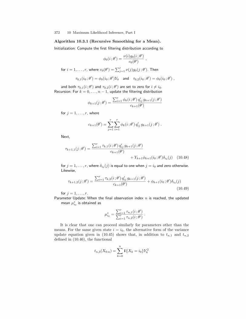
372 10 Maximum Likelihood Inference, Part I

Algorithm 10.3.1 (Recursive Smoothing for a Mean).

Initialization: Compute the first filtering distribution according to

φ0(i ; θ′) =ν(i)g0(i ; θ′)

c0(θ′),

for i = 1, . . . , r, where c0(θ′) =∑rj=1 ν(j)g0(j ; θ′). Then

τ0,1(i0 ; θ′) = φ0(i0 ; θ′)Y0 and τ0,2(i0 ; θ′) = φ0(i0 ; θ′) ,

and both τ0,1(i ; θ′) and τ0,2(i ; θ′) are set to zero for i 6= i0.Recursion: For k = 0, . . . , n− 1, update the filtering distribution

φk+1(j ; θ′) =

∑ri=1 φk(i ; θ′) q′ij gk+1(j ; θ′)

ck+1(θ′)

for j = 1, . . . , r, where

ck+1(θ′) =r∑j=1

r∑i=1

φk(i ; θ′) q′ij gk+1(j ; θ′) .

Next,

τk+1,1(j ; θ′) =

∑ri=1 τk,1(i ; θ′) q′ij gk+1(j ; θ′)

ck+1(θ′)+ Yk+1φk+1(i0 ; θ′)δi0(j) (10.48)

for j = 1, . . . , r, where δi0(j) is equal to one when j = i0 and zero otherwise.Likewise,

τk+1,2(j ; θ′) =

∑ri=1 τk,2(i ; θ′) q′ij gk+1(j ; θ′)

ck+1(θ′)+ φk+1(i0 ; θ′)δi0(j)

(10.49)for j = 1, . . . , r.

Parameter Update: When the final observation index n is reached, the updatedmean µ∗i0 is obtained as

µ∗i0 =∑ri=1 τn,1(i ; θ′)∑ri=1 τn,2(i ; θ′)

.

It is clear that one can proceed similarly for parameters other than themeans. For the same given state i = i0, the alternative form of the varianceupdate equation given in (10.45) shows that, in addition to tn,1 and tn,2defined in (10.46), the functional

tn,3(X0:n) =n∑k=0

1Xk = i0Y 2k

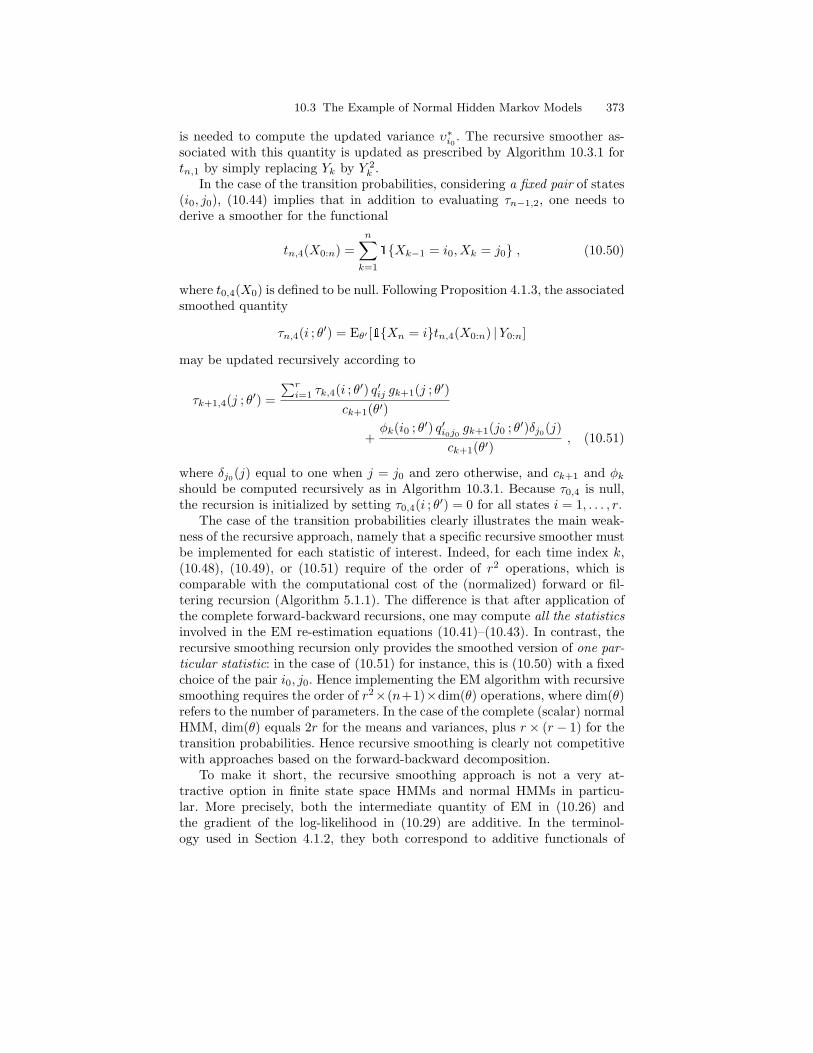
10.3 The Example of Normal Hidden Markov Models 373

is needed to compute the updated variance υ∗i0 . The recursive smoother as-sociated with this quantity is updated as prescribed by Algorithm 10.3.1 fortn,1 by simply replacing Yk by Y 2

k .In the case of the transition probabilities, considering a fixed pair of states

(i0, j0), (10.44) implies that in addition to evaluating τn−1,2, one needs toderive a smoother for the functional

tn,4(X0:n) =n∑k=1

1Xk−1 = i0, Xk = j0 , (10.50)

where t0,4(X0) is defined to be null. Following Proposition 4.1.3, the associatedsmoothed quantity

τn,4(i ; θ′) = Eθ′ [1Xn = itn,4(X0:n) |Y0:n]

may be updated recursively according to

τk+1,4(j ; θ′) =

∑ri=1 τk,4(i ; θ′) q′ij gk+1(j ; θ′)

ck+1(θ′)

+φk(i0 ; θ′) q′i0j0 gk+1(j0 ; θ′)δj0(j)

ck+1(θ′), (10.51)

where δj0(j) equal to one when j = j0 and zero otherwise, and ck+1 and φkshould be computed recursively as in Algorithm 10.3.1. Because τ0,4 is null,the recursion is initialized by setting τ0,4(i ; θ′) = 0 for all states i = 1, . . . , r.

The case of the transition probabilities clearly illustrates the main weak-ness of the recursive approach, namely that a specific recursive smoother mustbe implemented for each statistic of interest. Indeed, for each time index k,(10.48), (10.49), or (10.51) require of the order of r2 operations, which iscomparable with the computational cost of the (normalized) forward or fil-tering recursion (Algorithm 5.1.1). The difference is that after application ofthe complete forward-backward recursions, one may compute all the statisticsinvolved in the EM re-estimation equations (10.41)–(10.43). In contrast, therecursive smoothing recursion only provides the smoothed version of one par-ticular statistic: in the case of (10.51) for instance, this is (10.50) with a fixedchoice of the pair i0, j0. Hence implementing the EM algorithm with recursivesmoothing requires the order of r2×(n+1)×dim(θ) operations, where dim(θ)refers to the number of parameters. In the case of the complete (scalar) normalHMM, dim(θ) equals 2r for the means and variances, plus r × (r − 1) for thetransition probabilities. Hence recursive smoothing is clearly not competitivewith approaches based on the forward-backward decomposition.

To make it short, the recursive smoothing approach is not a very at-tractive option in finite state space HMMs and normal HMMs in particu-lar. More precisely, both the intermediate quantity of EM in (10.26) andthe gradient of the log-likelihood in (10.29) are additive. In the terminol-ogy used in Section 4.1.2, they both correspond to additive functionals of

374 10 Maximum Likelihood Inference, Part I

the form tn+1(x0:n+1) = tn(x0:n) + sn(xn, xn+1). In such cases, smooth-ing approaches based on the forward-backward decompositions such as Al-gorithms 5.1.2 or 5.1.3 that evaluate the bivariate smoothing distributionsφk:k+1|n for k = 0, . . . , n − 1 are more efficient because they do not requirethat the functions skk=0,...,n−1 be specified. There are however some situa-tions in which the recursive smoothing approach developed in Section 4.1 andillustrated above in the case of normal HMMs may be useful.

• First, because it is recursive, it does not require that the intermediatecomputation results be stored, which is in sharp contrast with the othersmoothing approaches where either the forward or backward variables needto be stored. This is of course of interest when processing very large datasets.

• When the functional whose conditional expectation is to be evaluated isnot of the additive type, approaches based on the evaluation of bivariatesmoothing distributions are not applicable anymore. In contrast, recursivesmoothing stays feasible as long as the functional follows the general pat-tern of Definition 4.1.2. The most significant functional of practical interestthat is not additive is the second-order derivative of the log-likelihood func-tion. The use of recursive smoothing for this purpose will be illustrated ona simple example in Section 10.3.4.

Finally, another different motivation for computing either the intermediatequantity of EM or the gradient of the log-likelihood recursively has to dowith recursive estimation. As noted by several authors, including Le Glandand Mevel (1997), Collings and Ryden (1998), and Krishnamurthy and Yin(2002), being able to compute recursively the intermediate quantity of EM orthe gradient of the log-likelihood is a key step toward efficient recursive (alsocalled on-line or adaptive) parameter estimation approaches. It is importanthowever to understand that recursive computation procedures do not neces-sarily directly translate into recursive estimation approaches. Algorithm 10.3.1for instance describes how to compute the EM update of the mean µi givensome observations Y0, . . . , Yn and a fixed current parameter value θ = θ′. Inrecursive estimation on the other hand, once a new observation Yk is collected,the parameter estimate, θk say, needs to be updated. Using the equations ofAlgorithm 10.3.1 with θk substituted for θ′ is of course a natural idea, butnot one that is guaranteed to produce the desired result. This is precisely theobjective of works such as Le Gland and Mevel (1997) and Krishnamurthyand Yin (2002), to study if and when such recursive approaches do produceexpected results. It is fair to say that, as of today, this remains a largely openissue.

10.3.4 Computation of the Score and Observed Information

For reasons discussed above, computing the gradient of the log-likelihood isnot a difficult task in finite state space HMMs and should preferably be done

10.3 The Example of Normal Hidden Markov Models 375

using smoothing algorithms based on the forward-backward decomposition.The only new requirement is to evaluate the derivatives with respect to θthat appear in (10.29). In the case of the normal HMM, we already met theappropriate expressions in (10.40), as Fisher’s identity (10.12) implies thatthe gradient of the intermediate quantity at the current parameter estimatecoincides with the gradient of the log-likelihood. Hence

∂

∂µi`n(θ) =

1υi

n∑k=0

φk|n(i ; θ)(Yk − µi) ,

∂

∂υi`n(θ) = −1

2

n∑k=0

φk|n(i ; θ)[

1υi− (Yk − µi)2

υ2i

],

∂

∂qij`n(θ) =

n∑k=1

φk−1:k|n(i, j ; θ)qij

.

Recall also that the log-likelihood itself is directly available from the filteringrecursion, following (5.4).

Before considering the computation of the Hessian, we first illustrate theperformance of the optimization methods introduced in Section 10.1.3, whichonly require the evaluation of the log-likelihood and its gradient.

Example 10.3.2 (Binary Deconvolution Model). We consider the sim-ple binary deconvolution model of Cappe et al. (1999), which is somewhatrelated to the channel coding situation described in Example 1.3.2, exceptthat the channel is unknown. This model is of interest in digital communi-cations (see for instance Krishnamurthy and White, 1992; Kaleh and Vallet,1994; Fonollosa et al., 1997). It is given by

Yk =p∑i=0

hiBk−i +Nk , (10.52)

where Ykk≥0 is the observed sequence, Nkk≥0 is a stationary sequenceof white Gaussian noise with zero mean and variance υ, and Bkk≥0 is asequence of transmitted symbols. For simplicity, we assume that Bkk≥0 is abinary, i.e., Bk ∈ −1, 1, sequence of i.i.d. fair Bernoulli draws. We considerbelow that p = 1, so that to cast the model into the HMM framework, weonly need to define the state as the vector Xk = (Bk, Bk−1)t, which takes oneof the four possible values

s1def=(−1−1

), s2

def=(−1

1

), s3

def=(

1−1

), s4

def=(

11

).

Hence, upon defining the vector h def= (h0 h1)t of filter coefficients, we mayview (10.52) as a four-states normal HMM such that µi = stih and υi = υ fori = 1, . . . , 4. The transition matrix Q is entirely fixed by our assumption thatthe binary symbols are equiprobable, and is given by

376 10 Maximum Likelihood Inference, Part I

Q =

1/2 0 1/2 01/2 0 1/2 00 1/2 0 1/20 1/2 0 1/2

.

The model parameters to be estimated are thus the vector h of filter co-efficients and the common variance υ. For simplicity, we assume that thedistribution of the initial state X0 is known.

To make the connection with the general (unconstrained) normal hiddenMarkov model discussed previously, we need only take into account the factsthat ∇hµi = si and ∂υi/∂υ = 1, as all variances are equal. Hence, using thechain rule, the gradient of the intermediate quantity of EM may be evaluatedfrom (10.40) as

∇hQ(θ ; θ′) =4∑i=1

∂

∂µiQ(θ ; θ′)∇hµi

=1υ

4∑i=1

n∑k=0

φk|n(i ; θ′)(Yksi − sistih) (10.53)

and

∂

∂υQ(θ ; θ′) =

4∑i=1

∂

∂υiQ(θ ; θ′)

∂υi∂υ

= −12

[n

υ−

4∑i=1

n∑k=0

φk|n(i ; θ′)(Yk − stih)2

υ2

]. (10.54)

The M-step update equations (10.41) and (10.42) of the EM algorithm shouldthus be replaced by

h∗ =

[4∑i=1

n∑k=0

φk|n(i ; θ′)sisti

]−1 [ 4∑i=1

n∑k=0

φk|n(i ; θ′)Yksi

],

υ∗ =1n

4∑i=1

n∑k=0

φk|n(i ; θ′)(Yk − stih∗)2

=1n

n∑k=0

Y 2k −

[4∑i=1

n∑k=0

φk|n(i ; θ′)Yksi

]th∗

.

For computing the log-likelihood gradient, we may resort to Fisher’s iden-tity, setting θ = θ′ in (10.53) and (10.54) to obtain ∇h`n(θ′) and ∂

∂υ `n(θ′) ,respectively.

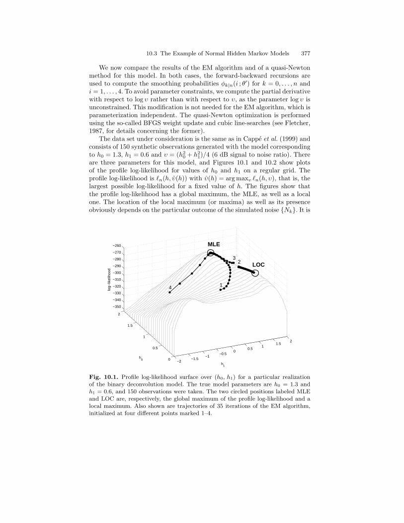
10.3 The Example of Normal Hidden Markov Models 377

We now compare the results of the EM algorithm and of a quasi-Newtonmethod for this model. In both cases, the forward-backward recursions areused to compute the smoothing probabilities φk|n(i ; θ′) for k = 0, . . . , n andi = 1, . . . , 4. To avoid parameter constraints, we compute the partial derivativewith respect to log υ rather than with respect to υ, as the parameter log υ isunconstrained. This modification is not needed for the EM algorithm, which isparameterization independent. The quasi-Newton optimization is performedusing the so-called BFGS weight update and cubic line-searches (see Fletcher,1987, for details concerning the former).

The data set under consideration is the same as in Cappe et al. (1999) andconsists of 150 synthetic observations generated with the model correspondingto h0 = 1.3, h1 = 0.6 and υ = (h2

0 + h21)/4 (6 dB signal to noise ratio). There

are three parameters for this model, and Figures 10.1 and 10.2 show plotsof the profile log-likelihood for values of h0 and h1 on a regular grid. Theprofile log-likelihood is `n(h, υ(h)) with υ(h) = arg maxv `n(h, υ), that is, thelargest possible log-likelihood for a fixed value of h. The figures show thatthe profile log-likelihood has a global maximum, the MLE, as well as a localone. The location of the local maximum (or maxima) as well as its presenceobviously depends on the particular outcome of the simulated noise Nk. It is

−2−1.5

−1−0.5

00.5

11.5

2

0

0.5

1

1.5

2

−350

−340

−330

−320

−310

−300

−290

−280

−270

−260

LOC23

h1

1

MLE

4

h0

log−

likel

ihoo

d

Fig. 10.1. Profile log-likelihood surface over (h0, h1) for a particular realizationof the binary deconvolution model. The true model parameters are h0 = 1.3 andh1 = 0.6, and 150 observations were taken. The two circled positions labeled MLEand LOC are, respectively, the global maximum of the profile log-likelihood and alocal maximum. Also shown are trajectories of 35 iterations of the EM algorithm,initialized at four different points marked 1–4.

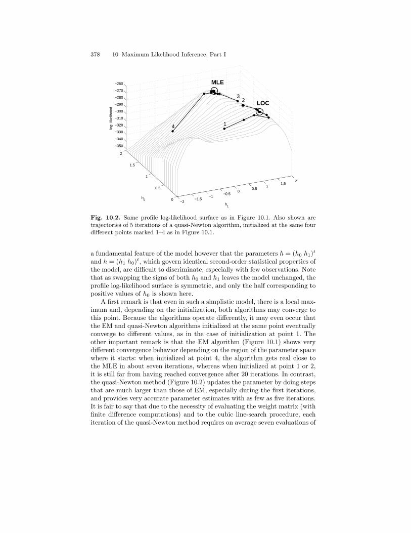
378 10 Maximum Likelihood Inference, Part I

−2−1.5

−1−0.5

00.5

11.5

2

0

0.5

1

1.5

2

−350

−340

−330

−320

−310

−300

−290

−280

−270

−260

LOC23

h1

1

MLE

4

h0

log−

likel

ihoo

d

Fig. 10.2. Same profile log-likelihood surface as in Figure 10.1. Also shown aretrajectories of 5 iterations of a quasi-Newton algorithm, initialized at the same fourdifferent points marked 1–4 as in Figure 10.1.

a fundamental feature of the model however that the parameters h = (h0 h1)t

and h = (h1 h0)t, which govern identical second-order statistical properties ofthe model, are difficult to discriminate, especially with few observations. Notethat as swapping the signs of both h0 and h1 leaves the model unchanged, theprofile log-likelihood surface is symmetric, and only the half corresponding topositive values of h0 is shown here.

A first remark is that even in such a simplistic model, there is a local max-imum and, depending on the initialization, both algorithms may converge tothis point. Because the algorithms operate differently, it may even occur thatthe EM and quasi-Newton algorithms initialized at the same point eventuallyconverge to different values, as in the case of initialization at point 1. Theother important remark is that the EM algorithm (Figure 10.1) shows verydifferent convergence behavior depending on the region of the parameter spacewhere it starts: when initialized at point 4, the algorithm gets real close tothe MLE in about seven iterations, whereas when initialized at point 1 or 2,it is still far from having reached convergence after 20 iterations. In contrast,the quasi-Newton method (Figure 10.2) updates the parameter by doing stepsthat are much larger than those of EM, especially during the first iterations,and provides very accurate parameter estimates with as few as five iterations.It is fair to say that due to the necessity of evaluating the weight matrix (withfinite difference computations) and to the cubic line-search procedure, eachiteration of the quasi-Newton method requires on average seven evaluations of

10.3 The Example of Normal Hidden Markov Models 379

the log-likelihood and its gradient, which means in particular seven instancesof the forward-backward procedure. From a computational point of view, thetime needed to run the 5 iterations of the quasi-Newton method in this ex-ample is thus roughly equivalent to that required for 35 iterations of the EMalgorithm.

As discussed earlier, computing the observed information in HMMs is moreinvolved, as the only computationally feasible option consists in adopting therecursive smoothing framework of Proposition 4.1.3. Rather than embarkinginto the general normal HMM case, we consider another simpler illustrativeexample where the parameter of interest is scalar.

Example 10.3.3. Consider a simplified version of the ion channel model (Ex-ample 1.3.5) in which the state space X is composed of two states that are (byconvention) labeled 0 and 1, and g(0, y) and g(1, y) respectively correspondto the N(0, υ) and N(1, υ) distributions. This model may also be interpretedas a state space model in which

Yk = Xk + Vk ,

where Vk is an i.i.d. N(0, υ)-distributed sequence, independent of theMarkov chain Xk, which takes its values in the set 0, 1. The transitionmatrix Q of Xk is parameterized in the form

Q =(

ρ0 1− ρ0

1− ρ1 ρ1

).

It is also most logical in this case to assume that the initial distribution νof X0 coincides with the stationary distribution associated with Q, that is,ν(0) = ρ0/(ρ0 + ρ1) and ν(1) = ρ1/(ρ0 + ρ1). In this model, the distributionsof holding times (number of consecutive steps k for which Xk stays constant)have geometric distributions with expectations (1− ρ0)−1 and (1− ρ1)−1 forstates 0 and 1, respectively.

We now focus on the computation of the derivatives of the log-likelihoodin the model of Example 10.3.3 with respect to the transition parameters ρ0

and ρ1. As they play a symmetric role, it is sufficient to consider, say, ρ0 only.The variance υ is considered as fixed so that the only quantities that dependon the parameter ρ0 are the initial distribution ν and the transition matrixQ. We will, as usual, use the simplified notation gk(x) rather than g(x, Yk)to denote the Gaussian density function (2πυ)−1/2 exp−(Yk − x)2/(2υ) forx ∈ 0, 1. Furthermore, in order to simplify the expressions below, we alsoomit to indicate explicitly the dependence with respect to ρ0 in the rest ofthis section. Fisher’s identity (10.12) reduces to

∂

∂ρ0`n = E

[∂

∂ρ0log ν(X0) +

n−1∑k=0

∂

∂ρ0log qXkXk+1

∣∣∣∣∣ Y0:n

],

380 10 Maximum Likelihood Inference, Part I

where the notation qij refers to the element in the (1+i)-th row and (1+j)-thcolumn of the matrix Q (in particular, q00 and q11 are alternative notationsfor ρ0 and ρ1). We are thus in the framework of Proposition 4.1.3 with asmoothing functional tn,1 defined by

t0,1(x) =∂

∂ρ0log ν(x) ,

sk,1(x, x′) =∂

∂ρ0log qxx′ for k ≥ 0 ,

where the multiplicative functions mk,1k≥0 are equal to 1. Straightforwardcalculations yield

t0,1(x) = (ρ0 + ρ1)−1

[ρ1

ρ0δ0(x)− δ1(x)

],

sk,1(x, x′) =1ρ0δ(0,0)(x, x′)−

11− ρ0

δ(0,1)(x, x′) .

Hence a first recursion, following Proposition 4.1.3.

Algorithm 10.3.4 (Computation of the Score in Example 10.3.3).

Initialization: Compute c0 =∑1i=0 ν(i)g0(i) and, for i = 0, 1,

φk(i) = c−10 ν(i)g0(i) ,

τ0,1(i) = t0,1(i)φ0(i) .

Recursion: For k = 0, 1, . . . , compute ck+1 =∑1i=0

∑1j=0 φk(i)qijgk(j) and, for

j = 0, 1,

φk+1(j) = c−1k+1

1∑i=0

φk(i)qijgk(j) ,

τk+1,1(j) = c−1k+1

1∑i=0

τk,1(i)qijgk+1(j)

+ φk(0)gk+1(0)δ0(j)− φk(0)gk+1(1)δ1(j).

At each index k, the log-likelihood is available via `k =∑kl=0 log cl, and its

derivative with respect to ρ0 may be evaluated as

∂

∂ρ0`k =

1∑i=0

τk,1(i) .

10.3 The Example of Normal Hidden Markov Models 381

For the second derivative, Louis’ identity (10.14) shows that

∂2

∂ρ20

`n +

∂

∂ρ0`n

2

= E

[∂2

∂ρ20

log ν(X0) +n−1∑k=0

∂2

∂ρ20

log qXkXk+1

∣∣∣∣∣ Y0:n

]

+ E

( ∂

∂ρ0log ν(X0) +

n−1∑k=0

∂

∂ρ0log qXkXk+1

)2∣∣∣∣∣∣ Y0:n

. (10.55)

The first term on the right-hand side of (10.55) is very similar to the caseof τn,1 considered above, except that we now need to differentiate the func-tions twice, replacing t0,1 and sk,1 by ∂

∂ρ0t0,1 and ∂

∂ρ0sk,1, respectively. The

corresponding smoothing functional tn,2 is thus now defined by

t0,2(x) = −ρ1(2ρ0 + ρ1)ρ2

0(ρ0 + ρ1)2δ0(x) +

1(ρ0 + ρ1)2

δ1(x) ,

sk,2(x, x′) = − 1ρ2

0

δ(0,0)(x, x′)−1

(1− ρ0)2δ(0,1)(x, x′) .

The second term on the right-hand side of (10.55) is more difficult, and weneed to proceed as in Example 4.1.4: the quantity of interest may be rewrittenas the conditional expectation of

tn,3(x0:n) =

[t0,1(x0) +

n−1∑k=0

sk,1(xk, xk+1)

]2

.

Expanding the square in this equation yields the update formula

tk+1,3(x0:k+1) = tk,3(x0:k) + s2k,1(xk, xk+1) + 2tk,1(x0:k)sk,1(xk, xk+1) .

Hence tk,1 and tk,3 jointly are of the form prescribed by Definition 4.1.2 withincremental additive functions sk,3(x, x′) = s2

k,1(x, x′) and multiplicative up-dates mk,3(x, x′) = 2sk,1(x, x′). As a consequence, the following smoothingrecursion holds.

Algorithm 10.3.5 (Computation of the Observed Information in Ex-ample 10.3.3).

Initialization: For i = 0, 1,

τ0,2(i) = t0,2(i)φ0(i) .

τ0,3(i) = t20,1(i)φ0(i) .

Recursion: For k = 0, 1, . . . , compute for j = 0, 1,

382 10 Maximum Likelihood Inference, Part I

τk+1,2(j) = c−1k+1

1∑i=0

τk,2(i)qijgk+1(j)

− 1ρ0φk(0)gk+1(0)δ0(j)− 1

(1− ρ0)φk(0)gk+1(1)δ1(j)

,

τ0,3(j) = c−1k+1

1∑i=0

τk,3(i)qijgk+1(j)

+ 2 [τk,1(0)gk+1(0)δ0(j)− τk,1(0)gk+1(1)δ1(j)]

+1ρ0φk(0)gk+1(0)δ0(j) +

1(1− ρ0)

φk(0)gk+1(1)δ1(j)

.

At each index k, the second derivative of the log-likelihood satisfies

∂2

∂ρ20

`k +(

∂

∂ρ0`k

)2

=1∑i=0

τk,2(i) +1∑i=0

τk,3(i) ,

where the second term on the left-hand side may be evaluated in the same recur-sion, following Algorithm 10.3.4.

To illustrate the results obtained with Algorithms 10.3.4–10.3.5, we con-sider the model with parameters ρ0 = 0.95, ρ1 = 0.8, and υ = 0.1 (usingthe notations introduced in Example 10.3.3). Figure 10.3 displays the typi-cal aspect of two sequences of length 200 simulated under slightly differentvalues of ρ0. One possible use of the output of Algorithms 10.3.4–10.3.5 con-sists in testing for changes in the parameter values. Indeed, under conditionsto be detailed in Chapter 12 (and which hold here), the normalized scoren−1/2 ∂

∂ρ0`n satisfies a central limit theorem with variance given by the limit

of the normalized information −n−1(∂2/∂ρ20)`n. Hence it is expected that

Rn =∂∂ρ0

`n√− ∂2

∂ρ20`n

be asymptotically N(0, 1)-distributed under the null hypothesis that ρ0 isindeed equal to the value used for computing the score and information re-cursively with Algorithms 10.3.4–10.3.5.

Figure 10.4 displays the empirical quantiles of Rn against normal quantilesfor n = 200 and n =1,000. For the longer sequences (n =1,000), the resultis clearly as expected with a very close fit to the normal quantiles. Whenn = 200, asymptotic normality is not yet reached and there is a significantbias toward high values of Rn. Looking back at Figure 10.3, even if υ was equalto zero—or in other words, if we were able to identify without ambiguity the0 and 1 states from the data—there would not be much information aboutρ0 to be gained from runs of length 200: when ρ0 = 0.95 and ρ1 = 0.8, the

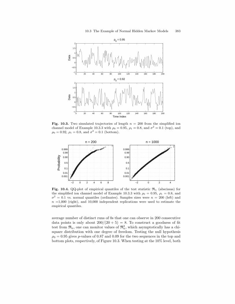
10.3 The Example of Normal Hidden Markov Models 383

0 20 40 60 80 100 120 140 160 180 200−1

−0.5

0

0.5

1

1.5

2

ρ0 = 0.92

Time Index

Dat

a

0 20 40 60 80 100 120 140 160 180 200−1

−0.5

0

0.5

1

1.5

2

ρ0 = 0.95

Dat

a

Fig. 10.3. Two simulated trajectories of length n = 200 from the simplified ionchannel model of Example 10.3.3 with ρ0 = 0.95, ρ1 = 0.8, and σ2 = 0.1 (top), andρ0 = 0.92, ρ1 = 0.8, and σ2 = 0.1 (bottom).

−2 0 2 4

0.001 0.01

0.1

0.5

0.90

0.990.999

n = 1000

−2 0 2 4 6 8

0.001 0.01

0.1

0.5

0.90

0.990.999

Pro

babi

lity

n = 200

Fig. 10.4. QQ-plot of empirical quantiles of the test statistic Rn (abscissas) forthe simplified ion channel model of Example 10.3.3 with ρ0 = 0.95, ρ1 = 0.8, andσ2 = 0.1 vs. normal quantiles (ordinates). Samples sizes were n = 200 (left) andn =1,000 (right), and 10,000 independent replications were used to estimate theempirical quantiles.

average number of distinct runs of 0s that one can observe in 200 consecutivedata points is only about 200/(20 + 5) = 8. To construct a goodness of fittest from Rn, one can monitor values of R2

n, which asymptotically has a chi-square distribution with one degree of freedom. Testing the null hypothesisρ0 = 0.95 gives p-values of 0.87 and 0.09 for the two sequences in the top andbottom plots, respectively, of Figure 10.3. When testing at the 10% level, both

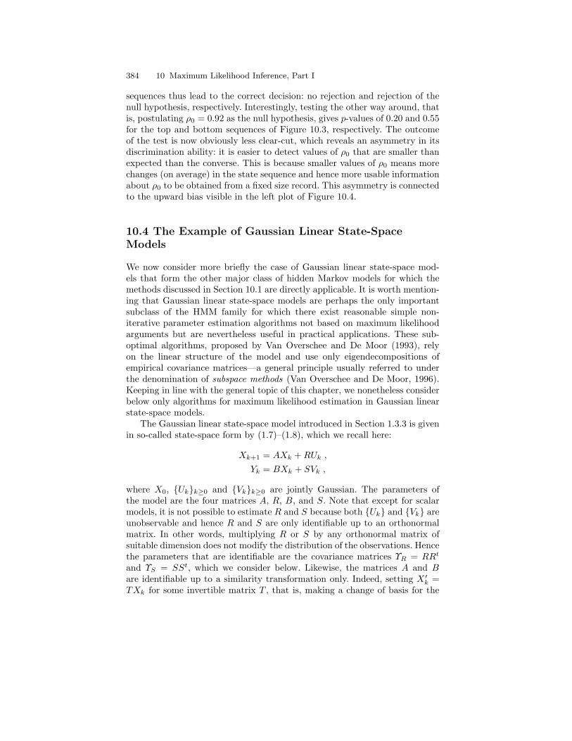
384 10 Maximum Likelihood Inference, Part I

sequences thus lead to the correct decision: no rejection and rejection of thenull hypothesis, respectively. Interestingly, testing the other way around, thatis, postulating ρ0 = 0.92 as the null hypothesis, gives p-values of 0.20 and 0.55for the top and bottom sequences of Figure 10.3, respectively. The outcomeof the test is now obviously less clear-cut, which reveals an asymmetry in itsdiscrimination ability: it is easier to detect values of ρ0 that are smaller thanexpected than the converse. This is because smaller values of ρ0 means morechanges (on average) in the state sequence and hence more usable informationabout ρ0 to be obtained from a fixed size record. This asymmetry is connectedto the upward bias visible in the left plot of Figure 10.4.

10.4 The Example of Gaussian Linear State-SpaceModels

We now consider more briefly the case of Gaussian linear state-space mod-els that form the other major class of hidden Markov models for which themethods discussed in Section 10.1 are directly applicable. It is worth mention-ing that Gaussian linear state-space models are perhaps the only importantsubclass of the HMM family for which there exist reasonable simple non-iterative parameter estimation algorithms not based on maximum likelihoodarguments but are nevertheless useful in practical applications. These sub-optimal algorithms, proposed by Van Overschee and De Moor (1993), relyon the linear structure of the model and use only eigendecompositions ofempirical covariance matrices—a general principle usually referred to underthe denomination of subspace methods (Van Overschee and De Moor, 1996).Keeping in line with the general topic of this chapter, we nonetheless considerbelow only algorithms for maximum likelihood estimation in Gaussian linearstate-space models.

The Gaussian linear state-space model introduced in Section 1.3.3 is givenin so-called state-space form by (1.7)–(1.8), which we recall here:

Xk+1 = AXk +RUk ,

Yk = BXk + SVk ,

where X0, Ukk≥0 and Vkk≥0 are jointly Gaussian. The parameters ofthe model are the four matrices A, R, B, and S. Note that except for scalarmodels, it is not possible to estimate R and S because both Uk and Vk areunobservable and hence R and S are only identifiable up to an orthonormalmatrix. In other words, multiplying R or S by any orthonormal matrix ofsuitable dimension does not modify the distribution of the observations. Hencethe parameters that are identifiable are the covariance matrices ΥR = RRt

and ΥS = SSt, which we consider below. Likewise, the matrices A and Bare identifiable up to a similarity transformation only. Indeed, setting X ′k =TXk for some invertible matrix T , that is, making a change of basis for the

10.4 The Example of Gaussian Linear State-Space Models 385

state process, it is straightforward to check that the joint process (X ′k, Yk)satisfies the model assumptions with TAT−1, BT−1, and TR replacing A, B,and R, respectively. Nevertheless, we work with A and B in the algorithmbelow. If a unique representation is desired, one may use, for instance, thecompanion form of A given its eigenvalues; this matrix may contain complexentries though. As in the case of finite state space HMMs (Section 10.2.2), itis not sensible to consider the initial covariance matrix Σν as an independentparameter when using a single observed sequence. On the other hand, for suchmodels it is very natural to assume that Σν is associated with the stationarydistribution of Xk. Except for the particular case of the scalar AR(1) modelhowever (to be discussed in Example 11.1.2), this option typically renders theEM update equations non-explicit and it is thus standard practice to treatΣν as a fixed matrix unrelated to the parameters (Ghosh, 1989). We shallalso assume that both ΥR and ΥS are full rank covariance matrices so thatall Gaussian distributions admit densities with respect to (multi-dimensional)Lebesgue measure.

10.4.1 The Intermediate Quantity of EM

With the previous notations, the intermediate quantity Q(θ ; θ′) of EM, de-fined in (10.26), may be expressed as

− 12

Eθ′

[n log |ΥR|+

n−1∑k=0

(Xk+1 −AXk)tΥ−1R (Xk+1 −AXk)

∣∣∣∣∣ Y0:n

]

− 12

Eθ′

[(n+ 1) log |ΥS |+

n∑k=0

(Yk −BXk)tΥ−1S (Yk −BXk)

∣∣∣∣∣ Y0:n

],

(10.56)

up to terms that do not depend on the parameters. In order to elicit the M-stepequations or to compute the score, we differentiate (10.56) using elementaryperturbation calculus as well as the identity∇C log |C| = C−t for an invertiblematrix C—which is a consequence of the adjoint representation of the inverse(Horn and Johnson, 1985, Section 0.8.2):

∇AQ(θ ; θ′) = −Υ−1R Eθ′

[n−1∑k=0

(AXkXtk −Xk+1X

tk)

∣∣∣∣∣ Y0:n

], (10.57)

∇Υ−1RQ(θ ; θ′) = −1

2

−nΥR (10.58)

+ Eθ′

[n−1∑k=0

(Xk+1 −AXk)(Xk+1 −AXk)t∣∣∣∣∣ Y0:n

],

∇BQ(θ ; θ′) = −Υ−1S Eθ′

[n∑k=0

(BXkXtk − YkXt

k)

∣∣∣∣∣ Y0:n

], (10.59)

386 10 Maximum Likelihood Inference, Part I

∇Υ−1SQ(θ ; θ′) = −1

2

−(n+ 1)ΥS (10.60)

+ Eθ′

[n∑k=0

(Yk −BXk)(Yk −BXk)t∣∣∣∣∣ Y0:n

].

Note that in the expressions above, we differentiate with respect to the inversesof ΥR and ΥS rather than with respect to the covariance matrices themselves,which is equivalent, because we assume both of the covariance matrices to bepositive definite, but yields simpler formulas. Equating all derivatives simul-taneously to zero defines the EM update of the parameters. We will denotethese updates by A∗, B∗, Υ ∗R, and Υ ∗S , respectively. To write them down, wewill use the notations introduced in Chapter 5: Xk|n(θ′) = Eθ′ [Xk |Y0:n] andΣk|n(θ′) = Eθ′ [XkX

′k |Y0:n]− Xk|n(θ′)Xt

k|n(θ′), where we now indicate explic-itly that these first two smoothing moments indeed depend on the currentestimates of the model parameters (they also depend on the initial covariancematrix Σν , but we ignore this fact here because this quantity is considered asbeing fixed). We also need to evaluate the conditional covariances

Ck,k+1|n(θ′) def= Covθ′ [Xk, Xk+1 |Y0:n]

= Eθ′ [XkXtk+1 |Y0:n]− Xk|n(θ′)Xt

k+1|n(θ′) .

For Gaussian models, the latter expression coincides with the definition givenin (5.99), and hence one may use expression (5.100) to evaluate Ck,k+1|n(θ′)during the final forward recursion of Algorithm 5.2.15.

With these notations, the EM update equations are given by

A∗ =

[n−1∑k=0

Ck,k+1|n(θ′) + Xk|n(θ′)Xtk+1|n(θ′)

]t(10.61)

[n−1∑k=0

Σk|n(θ′) + Xk|n(θ′)Xtk|n(θ′)

]−1

,

Υ ∗R =1n

n−1∑k=0

[Σk+1|n(θ′) + Xk+1|n(θ′)Xt

k+1|n(θ′)]

(10.62)

−A∗[Ck,k+1|n(θ′) + Xk|n(θ′)Xt

k+1|n(θ′)]

,

B∗ =

[n∑k=0

Xk|n(θ′)Y tk

]t(10.63)

[n∑k=0

Σk|n(θ′) + Xk|n(θ′)Xtk|n(θ′)

]−1

,

10.4 The Example of Gaussian Linear State-Space Models 387

Υ ∗S =1

n+ 1

n∑k=0

[YkY

tk −B∗Xk|n(θ′)Y tk

]. (10.64)

In obtaining the covariance update, we used the same remark that made itpossible to rewrite, in the case of normal HMMs, (10.42) as (10.45).

10.4.2 Recursive Implementation

As in the case of finite state space HMMs, it is possible to implement the pa-rameter update equations (10.61)–(10.64) or to compute the gradient (10.57)–(10.60) of the log-likelihood recursively in n. Here we only sketch the generalprinciples and refer to the paper by Elliott and Krishnamurthy (1999) inwhich the details of the EM re-estimation equations are worked out. Proceed-ing as in Section 4.1, it is clear that all expressions under consideration maybe rewritten term by term as the expectation2 E[tn(X0:n) |Y0:n] of well chosenadditive functionals tn. More precisely, the functionals of interest are of theform tn(x0:n) = t0(x0) +

∑n−1k=0 sk(xk, xk+1), where the individual terms in

the sum are of one of the types

sk−1,1(xk) = htkxk , (10.65)

sk−1,2(xk) = xtkMkxk , (10.66)

sk−1,3(xk−1, xk) = xtk−1Tk−1xk , (10.67)

and hkk≥0, Mkk≥0, and Tkk≥0, respectively, denote sequences of vectorsand matrices with dimension that of the state vectors (dx) and which maydepend on the model parameters or on the observations.

For illustration purposes, we focus on the example of (10.63): the firstfactor on the right-hand side of (10.63) is a matrix whose ij elements (ithrow, jth column) corresponds to E[

∑nk=0 h

tkXk |Y0:n] for the particular choice

hk =(

0 . . . 0 Yk(i) 0 . . . 0)t

.1 . . . j − 1 j j + 1 . . . dx

(10.68)

Likewise, the ij element of the second factor on the right-hand side of (10.63)—before inverting the matrix—corresponds to the expectation of a functionalof the second of the three types above with Mk being a matrix of zeros exceptfor a unit entry at position ij.

Let τn,1 denote the expectation E[∑nk=0 h

tkXk |Y0:n] for an additive func-

tional of the first type given in (10.65). To derive a recursion for τn,1, we usethe innovation decomposition (Section 5.2.2) to obtain

2Note that in this section, we omit to indicate explicitly the dependence withrespect to the model parameters to alleviate the notations.

388 10 Maximum Likelihood Inference, Part I

τn+1,1def= Eθ′

[n+1∑k=0

htkXk

∣∣∣∣∣Y0:n+1

]= htn+1Xn+1|n+1

+n∑k=0

htk

(Xk|n + E[Xkε

tn+1]Γ−1

n+1εn+1

)= htn+1Xn+1|n+1 + E

[n∑k=0

htkXk

∣∣∣∣∣Y0:n

]

+

(n∑k=0

htkΣk|k−1Λtk Λ

tk+1 . . . Λtn

)︸ ︷︷ ︸

rn+1

BtΓ−1n+1εn+1 ,

where (5.93) was used to obtain the last expression, which also features thenotation Λk = A −HkB with Hk being the Kalman (prediction) gain intro-duced in the statement of Algorithm 5.2.15. The term that we denoted byrn+1 is an intermediate quantity that has some similarities with the variablepk (or more precisely p0) that is instrumental in the disturbance smoothingalgorithm (Algorithm 5.2.15). The same key remark applies here as rn can becomputed recursively (in n) according to the equations

r0 = 0 ,

rn+1 =(rn + hnΣn|n−1

)Λtn for n ≥ 0 .

Hence the following recursive smoothing algorithm, which collects all neces-sary steps.

Algorithm 10.4.1 (Recursive Smoothing for a Linear Sum Func-tional).

Initialization: Apply the Kalman filtering recursion for k = 0 (Algorithm 5.2.13)and set

r0 = 0 ,

τ0 = E[ht0X0 |Y0] = ht0X0|0 .

Recursion: For n = 1, 2, . . . , run one step of the Kalman filtering and predictionrecursions (Algorithms 5.2.9 and 5.2.13) and compute

rn =(rn−1 + hn−1Σn−1|n−2

)Λtn−1 ,

τn = E

[n∑k=0

htkXk

∣∣∣∣∣Y0:n

]= htnXn|n + τn−1 + rnB

tΓ−1n εn .

10.5 Complements 389

Algorithm 10.4.1 illustrates the fact that as in the case of finite state spacemodels, recursive computation is in general less efficient than is forward-backward smoothing from a computational point of view: although Algo-rithm 10.4.1 capitalizes on a common framework formed by the Kalman filter-ing and prediction recursions, it does however require the update of a quantity(rn) that is specific to the choice of the sequence of vectors hkk≥0. To com-pute the first factor on the right-hand side of (10.63) for instance, one needsto apply the recursion of Algorithm 10.4.1 for the dy × dx possible choices ofhkk≥0 given by (10.68). Thus, except for low-dimensional models or partic-ular cases in which the system matrices A, ΥR, B, and ΥS are very sparse,recursive computation is usually not the method of choice for Gaussian linearstate-space models (see Elliott and Krishnamurthy, 1999, for a discussion ofthe complexity of the complete set of equations required to carry out the EMparameter update).

10.5 Complements

To conclude this chapter, we briefly return to an issue mentioned in Sec-tion 10.1.2 regarding the conditions that ensure that the EM iterations indeedconverge to stationary points of the likelihood.

10.5.1 Global Convergence of the EM Algorithm

As a consequence of Proposition 10.1.4, the EM algorithm described in Sec-tion 10.1.2 has the property that the log-likelihood function ` can never de-crease in an iteration. Indeed,

`(θi+1)− `(θi) ≥ Q(θi+1 ; θi)−Q(θi ; θi) ≥ 0 .

This class of algorithms, sometimes referred to as ascent algorithms (Luen-berger, 1984, Chapter 6), can be treated in a unified manner following a theorydeveloped mostly by Zangwill (1969). Wu (1983) showed that this general the-ory applies to the EM algorithm as defined above, as well as to some of itsvariants that he calls generalized EM (or GEM). The main result is a strongstability guarantee known as global convergence, which we discuss below.

We first need a mathematical formalism that describes the EM algorithm.This is done by identifying any homogeneous (in the iterations) iterative al-gorithm with a specific choice of a mapping M that associates θi+1 to θi.In the theory of Zangwill (1969), one indeed considers families of algorithmsby allowing for point-to-set maps M that associate a set M(θ′) ⊆ Θ to eachparameter value θ′ ∈ Θ. A specific algorithm in the family is such that θi+1

is selected in M(θi). In the example of EM, we may define M as

M(θ′) =θ ∈ Θ : Q(θ ; θ′) ≥ Q(θ ; θ′) for all θ ∈ Θ

, (10.69)

390 10 Maximum Likelihood Inference, Part I

that is, M(θ′) is the set of values θ that maximize Q(θ ; θ′) over Θ. UsuallyM(θ′) reduces to a singleton, and the mapping M is then simply a point-to-point map (a usual function from Θ to Θ). But the use of point-to-set mapsmakes it possible to deal also with cases where the intermediate quantity ofEM may have several global maxima, without going into the details of whatis done in such cases. We next need the following definition before stating themain convergence theorem.

Definition 10.5.1 (Closed Mapping). A map T from points of Θ to subsetsof Θ is said to be closed on a set S ⊆ Θ if for any converging sequences θii≥0

and θii≥0, the conditions

(a) θi → θ ∈ S,(b) θi → θ with θi ∈ T (θi) for all i ≥ 0,

imply that θ ∈ T (θ).

Note that for point-to-point maps, that is, if T (θ) is a singleton for all θ,the definition above is equivalent to the requirement that T be continuous onS. Definition 10.5.1 is thus a generalization of continuity for general (point-to-set) maps. We are now ready to state the main result, which is provedin Zangwill (1969, p. 91) or Luenberger (1984, p. 187).

Theorem 10.5.2 (Global Convergence Theorem). Let Θ be a subset ofRdθ and let θii≥0 be a sequence generated by θi+1 ∈ T (θi) where T is apoint-to-set map on Θ. Let S ⊆ Θ be a given “solution” set and suppose that

(1) the sequence θii≥0 is contained in a compact subset of Θ;(2) T is closed over Θ \ S (the complement of S);(3) there is a continuous “ascent” function s on Θ such that s(θ) ≥ s(θ′) for

all θ ∈ T (θ′), with strict inequality for points θ′ that are not in S.

Then the limit of any convergent subsequence of θi is in the solution set S. Inaddition, the sequence of values of the ascent function, s(θi)i≥0, convergesmonotonically to s(θ?) for some θ? ∈ S.

The final statement of Theorem 10.5.2 should not be misinterpreted: thats(θi) converges to a value that is the image of a point in S is a simpleconsequence of the first and third assumptions. It does however not implythat the sequence of parameters θi is itself convergent in the usual sense,but only that the limit points of θi have to be in the solution set S. Animportant property however is that because s(θi(l))l≥0 converges to s(θ?)for any convergent subsequence θi(l), all limit points of θi must be inthe set S? = θ ∈ Θ : s(θ) = s(θ?) (in addition to being in S). This latterstatement means that the sequence of iterates θi will ultimately approacha set of points that are “equivalent” as measured by the ascent function s.

The following general convergence theorem following the proof by Wu(1983) is a direct application of the previous theory to the case of EM.

10.5 Complements 391

Theorem 10.5.3. Suppose that in addition to the hypotheses of Proposi-tion 10.1.4 (Assumptions 10.1.3 as well as parts (a) and (b) of Proposi-tion 10.1.4), the following hold.

(i) H(θ ; θ′) is continuous in its second argument, θ′, on Θ.(ii) For any θ0, the level set Θ0 =

θ ∈ Θ : `(θ) ≥ `(θ0)

is compact and

contained in the interior of Θ.

Then all limit points of any instance θii≥0 of an EM algorithm initializedat θ0 are in L0 = θ ∈ Θ0 : ∇θ`(θ) = 0, the set of stationary points of ` withlog-likelihood larger than that of θ0. The sequence `(θi) of log-likelihoodsconverges monotonically to `? = `(θ?) for some θ? ∈ L0.

Proof. This is a direct application of Theorem 10.5.2 using L0 as the solu-tion set and ` as the ascent function. The first hypothesis of Theorem 10.5.2follows from (ii) and the third one from Proposition 10.1.4. The closednessassumption (2) follows from Proposition 10.1.4 and (i): for the EM mappingM defined in (10.69), θi ∈M(θi) amounts to the condition

Q(θi ; θi) ≥ Q(θ ; θi) for all θ ∈ Θ ,

which is also satisfied by the limits of the sequences θi and θi (if theseconverge) by continuity of the intermediate quantity Q, which follows fromthat of ` and H (note that it is here important that H be continuous withrespect to both arguments). Hence the EM mapping is indeed closed on Θ asa whole and Theorem 10.5.3 follows. ut

The assumptions of Proposition 10.1.4 as well as item (i) above are indeedvery mild in typical situations. Assumption (ii) however may be restrictive,even for models in which the EM algorithm is routinely used (such as thenormal HMMs introduced in Section 1.3.2, for which this assumption doesnot hold if the variances υi are allowed to be arbitrarily small). The practicalimplication of (ii) being violated is that the EM algorithm may fail to convergeto the stationary points of the likelihood for some particularly badly choseninitial points θ0.

Most importantly, the fact that θi+1 maximizes the intermediate quantityQ(· ; θi) of EM does in no way imply that, ultimately, `? is the global maximumof ` over Θ. There is even no guarantee that `? is a local maximum of the log-likelihood: it may well only be a saddle point (Wu, 1983, Section 2.1). Also,the convergence of the sequence `(θi) to `? does not automatically imply theconvergence of θi to a point θ?.

Pointwise convergence of the EM algorithm requires more stringent as-sumptions that are difficult to verify in practice. As an example, a simplecorollary of the global convergence theorem states that if the solution set Sin Theorem 10.5.2 is a single point, θ? say, then the sequence θi indeedconverges to θ? (Luenberger, 1984, p. 188). The sketch of the proof of thiscorollary is that every subsequence of θi has a convergent further subse-quence because of the compactness assumption (1), but such a subsequence

392 10 Maximum Likelihood Inference, Part I

admits s as an ascent function and thus converges to θ? by Theorem 10.5.2itself. In cases where the solution set is composed of several points, furtherconditions are needed to ensure that the sequence of iterates indeed convergesand does not cycle through different solution points.

In the case of EM, pointwise convergence of the EM sequence may beguaranteed under an additional condition given by Wu (1983) (see also Boyles,1983, for an equivalent result), stated in the following theorem.

Theorem 10.5.4. Under the hypotheses of Theorem 10.5.3, if

(iii) ‖θi+1 − θi‖ → 0 as i→∞,

then all limit points of θi are in a connected and compact subset of L? =θ ∈ Θ : `(θ) = `?, where `? is the limit of the log-likelihood sequence `(θi).

In particular, if the connected components of L? are singletons, then θiconverges to some θ? in L?.

Proof. The set of limit points of a bounded sequence θi with ‖θi+1−θi‖ → 0is connected and compact (Ostrowski, 1966, Theorem 28.1). The proof followsbecause under Theorem 10.5.2, the limit points of θi must belong to L?. ut

10.5.2 Rate of Convergence of EM

Even if one can guarantee that the EM sequence θi converges to some pointθ?, this limiting point can be either a local maximum, a saddle point, oreven a local minimum. The proposition below states conditions under whichthe stable stationary points of EM coincide with local maxima only (see alsoLange, 1995, Proposition 1, for a similar statement). We here consider thatthe EM mapping M is a point-to-point map, that is, that the maximizer inthe M-step is unique.

To understand the meaning of the term “stable”, consider the followingapproximation to the limit behavior of the EM sequence: it is sensible toexpect that if the EM mapping M is sufficiently regular in a neighborhood ofthe limiting fixed point θ?, the asymptotic behavior of the EM sequence θifollows the tangent linear dynamical system

(θi+1 − θ?) = M(θi)−M(θ?) ≈ ∇θM(θ?)(θi − θ?) . (10.70)

Here ∇θM(θ?) is called the rate matrix (see for instance Meng and Rubin,1991). A fixed point θ? is said to be stable if the spectral radius of ∇θM(θ?)is less than 1. In this case, the tangent linear system is asymptotically stablein the sense that the sequence ζi defined recursively by ζi+1 = ∇θM(θ?)ζi

tends to zero as n tends to infinity (for any choice of ζ0). The linear rateof convergence of EM is defined as the largest moduli of the eigenvalues of∇θM(θ?). This rate is an upper bound on the factors ρk that appear in (10.17).

10.5 Complements 393

Proposition 10.5.5. Under the assumptions of Theorem 10.1.6, assume thatQ(· ; θ) has a unique maximizer for all θ ∈ Θ and that, in addition,

H(θ?) = −∫∇2θ log f(x ; θ)

∣∣θ=θ?

p(x ; θ?)λ(dx) (10.71)

andG(θ?) = −

∫∇2θ log p(x ; θ)

∣∣θ=θ?

p(x ; θ?)λ(dx) (10.72)

are positive definite matrices for all stationary points of EM (i.e., such thatM(θ?) = θ?). Then for all such points, the following hold true.

(i) ∇θM(θ?) is diagonalizable and its eigenvalues are positive real numbers.(ii) The point θ? is stable for the mapping M if and only if it is a proper

maximizer of `(θ) in the sense that all eigenvalues of ∇2θ`(θ?) are nega-

tive.

Proof. The EM mapping is defined implicitly through the fact that M(θ′)maximizes Q(· ; θ′), which implies that∫

∇θ log f(x ; θ)|θ=M(θ′) p(x ; θ′)λ(dx) = 0 ,

using assumption (b) of Theorem 10.1.6. Careful differentiation of this relationat a point θ′ = θ?, which is such that M(θ?) = θ? and hence ∇θ `(θ)|θ=θ? = 0,gives (Dempster et al., 1977; Lange, 1995, see also)

∇θM(θ?) = [H(θ?)]−1[H(θ?) +∇2

θ`(θ?)],

where H(θ?) is defined in (10.71). The missing information principle—orLouis’ formula (see Proposition 10.1.6)—implies that G(θ?) = H(θ?)+∇2

θ`(θ?)is positive definite under our assumptions.

Thus ∇θM(θ?) is diagonalizable with positive eigenvalues that are thesame (counting multiplicities) as those of the matrix A? = I+B?, where B? =[H(θ?)]−1/2∇2

θ`(θ?)[H(θ?)]−1/2. Thus ∇θM(θ?) is stable if and only if B? hasnegative eigenvalues only. The Sylvester law of inertia (see for instance Hornand Johnson, 1985) shows that B? has the same inertia (number of positive,negative, and zero eigenvalues) as ∇2

θ`(θ?). Thus all of B?’s eigenvalues arenegative if and only if the same is true for ∇2

θ`(θ?), that is, if θ? is a propermaximizer of `. ut

The proof above implies that when θ? is stable, the eigenvalues of M(θ?) liein the interval (0, 1).

10.5.3 Generalized EM Algorithms

As discussed above, the type of convergence guaranteed by Theorem 10.5.3is rather weak but, on the other hand, this result is remarkable as it indeed

394 10 Maximum Likelihood Inference, Part I

covers not only the original EM algorithm proposed by Dempster et al. (1977)but a whole class of variants of the EM approach. One of the most usefulextensions of EM is the ECM (for expectation conditional maximization) byMeng and Rubin (1993), which addresses situations where direct maximizationof the intermediate quantity of EM is intractable. Assume for instance that theparameter vector θ consists of two sub-components θ1 and θ2, which are suchthat maximization of Q((θ1, θ2) ; θ′) with respect to θ1 or θ2 only (the othersub-component being fixed) is easy, whereas joint maximization with respectto θ = (θ1, θ2) is problematic. One may then use the following algorithm forupdating the parameter estimate at iteration i.

E-step: Compute Q((θ1, θ2) ; (θi1, θi2));

CM-step: Determine

θi+11 = arg max

θ1Q((θ1, θ

i2) ; (θi1, θ

i2)) ,

and thenθi+1

2 = arg maxθ2Q((θi+1

1 , θ2) ; (θi1, θi2)) .

It is easily checked that for this algorithm, (10.8) is still verified and thus `is an ascent function; this implies that Theorem 10.5.3 holds under the sameset of assumptions.

The example above is only the simplest case where the ECM approach maybe applied, and further extensions are discussed by Meng and Rubin (1993)as well as by Fessler and Hero (1995) and Meng and Van Dyk (1997).

10.5.4 Bibliographic Notes

The EM algorithm was popularized by the celebrated article of Dempster et al.(1977). It is generally admitted however that several published works predatedthis landmark paper by describing applications of the EM principle to somespecific cases (Meng and Van Dyk, 1997). Interestingly, the earliest example ofa complete EM strategy, which also includes convergence proofs (in additionto describing the forward-backward smoothing algorithm discussed in Chap-ter 3), is indeed the work by Baum et al. (1970) on finite state space HMMs,generalizing the idea put forward by Baum and Eagon (1967). This pioneer-ing contribution has been extended by authors such as Liporace (1982), whoshowed that the same procedure could be applied to other types of HMMs.The generality of the approach however was not fully recognized until Demp-ster et al. (1977) and Wu (1983) (who made the connection with the theoryof global convergence) showed that the convergence of the EM approach (andits generalizations) is guaranteed in great generality.

The fact that the EM algorithm may also be used, with minor modifi-cations, for MAP estimation was first mentioned by Dempster et al. (1977).Green (1990) illustrates a number of practical applications where this option

10.5 Complements 395

plays an important role. Perhaps the most significant of these is speech pro-cessing where MAP estimation, as first described by Gauvain and Lee (1994),is commonly used for the model adaptation task (that is, re-retraining fromsparse data of some previously trained models).

The ECM algorithm of Meng and Rubin (1993) (discussed Section 10.5.3)was also studied independently by Fessler and Hero (1995) under the nameSAGE (space-alternating generalized EM). Fessler and Hero (1995) also intro-duced the idea that in some settings it is advantageous to use different waysof augmenting the data, that is, different ways of writing the likelihood asin (10.1) depending on the parameter subset that one is trying to re-estimate;see also Meng and Van Dyk (1997) for further developments of this idea.

11

Maximum Likelihood Inference, Part II:Monte Carlo Optimization

This chapter deals with maximum likelihood parameter estimation for modelsin which the smoothing recursions of Chapter 3 cannot be implemented. Thetask is then considerably more difficult, as it is not even possible to evaluatethe likelihood to be maximized. Most of the methods applicable in such casesare reminiscent of the iterative optimization procedures (EM and gradientmethods) discussed in the previous chapter but rely on approximate smooth-ing computations based on some form of Monte Carlo simulation. In thiscontext, the methods covered in Chapters 6 and 7 for simulating the unob-servable sequence of states conditionally on the observations play a prominentrole.

It is important to distinguish the topic of this chapter with a distinct—although not entirely disconnected—problem. The methods discussed in theprevious chapters were all based on local exploration (also called hill-climbingstrategies) of the likelihood function. Such methods are typically unable toguarantee that the point reached at convergence is a global maximum of thefunction; indeed, it may well be a local maximum only or even a saddle point—see Section 10.5 for details regarding the EM algorithm. Many techniques havebeen proposed to overcome this significant difficulty, and most of them belongto a class of methods that Geyer (1996) describes as random search optimiza-tion. Typical examples are the so-called genetic and simulated annealing al-gorithms that both involve simulating random moves in the parameter space(see also Section 13.3, which describes a technique related to simulated an-nealing). In these approaches, the main motivation for using simulations (inparameter space and/or hidden variable space) is the hope to design morerobust optimization rules that can avoid local maxima.

The focus of the current chapter is different, however, as we examine belowmethods that can be considered as simulation-based extensions of approachesintroduced in the previous chapter. The primary objective is here to providetools for maximum likelihood inference also for the class of HMMs in whichexact smoothing is not available.

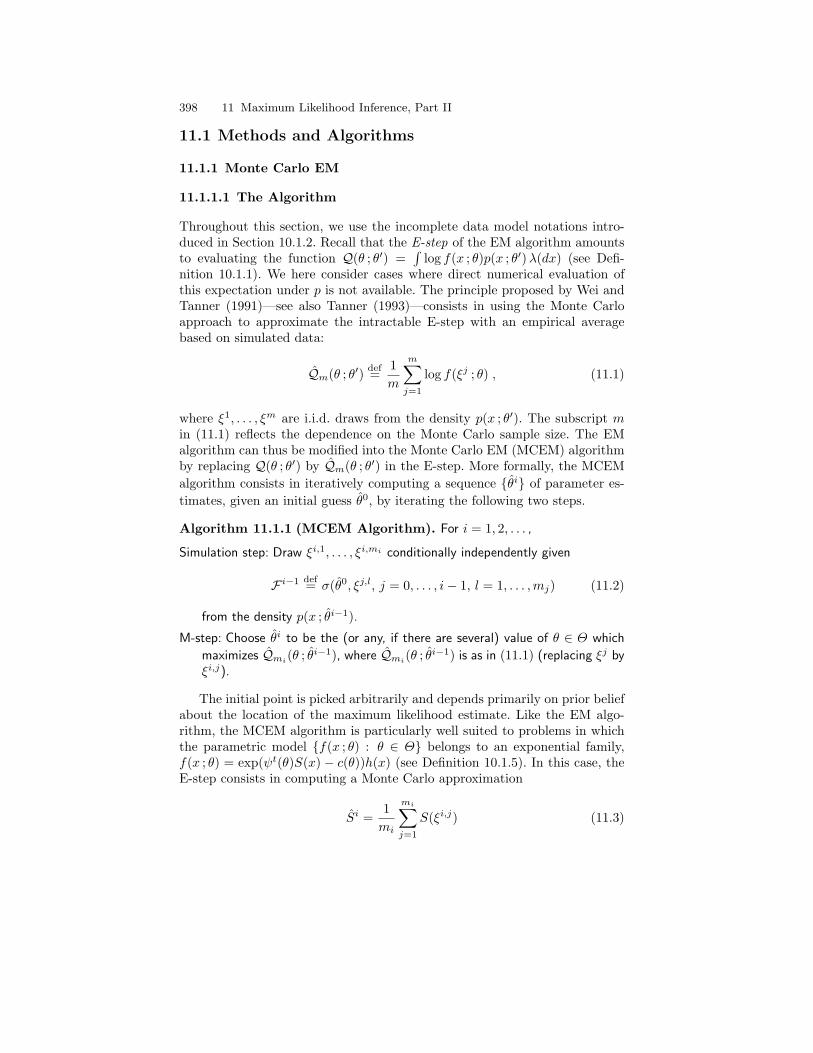
398 11 Maximum Likelihood Inference, Part II

11.1 Methods and Algorithms

11.1.1 Monte Carlo EM

11.1.1.1 The Algorithm

Throughout this section, we use the incomplete data model notations intro-duced in Section 10.1.2. Recall that the E-step of the EM algorithm amountsto evaluating the function Q(θ ; θ′) =

∫log f(x ; θ)p(x ; θ′)λ(dx) (see Defi-

nition 10.1.1). We here consider cases where direct numerical evaluation ofthis expectation under p is not available. The principle proposed by Wei andTanner (1991)—see also Tanner (1993)—consists in using the Monte Carloapproach to approximate the intractable E-step with an empirical averagebased on simulated data:

Qm(θ ; θ′) def=1m

m∑j=1

log f(ξj ; θ) , (11.1)

where ξ1, . . . , ξm are i.i.d. draws from the density p(x ; θ′). The subscript min (11.1) reflects the dependence on the Monte Carlo sample size. The EMalgorithm can thus be modified into the Monte Carlo EM (MCEM) algorithmby replacing Q(θ ; θ′) by Qm(θ ; θ′) in the E-step. More formally, the MCEMalgorithm consists in iteratively computing a sequence θi of parameter es-timates, given an initial guess θ0, by iterating the following two steps.

Algorithm 11.1.1 (MCEM Algorithm). For i = 1, 2, . . . ,

Simulation step: Draw ξi,1, . . . , ξi,mi conditionally independently given

F i−1 def= σ(θ0, ξj,l, j = 0, . . . , i− 1, l = 1, . . . ,mj) (11.2)

from the density p(x ; θi−1).

M-step: Choose θi to be the (or any, if there are several) value of θ ∈ Θ which

maximizes Qmi(θ ; θi−1), where Qmi(θ ; θi−1) is as in (11.1) (replacing ξj byξi,j).

The initial point is picked arbitrarily and depends primarily on prior beliefabout the location of the maximum likelihood estimate. Like the EM algo-rithm, the MCEM algorithm is particularly well suited to problems in whichthe parametric model f(x ; θ) : θ ∈ Θ belongs to an exponential family,f(x ; θ) = exp(ψt(θ)S(x)− c(θ))h(x) (see Definition 10.1.5). In this case, theE-step consists in computing a Monte Carlo approximation

Si =1mi

mi∑j=1

S(ξi,j) (11.3)

11.1 Methods and Algorithms 399

of the expectation∫S(x)p(x ; θi−1)λ(dx). The M-step then consists in op-

timizing the function θ 7→ ψt(θ)Si − c(θ). In many models, this function isconvex, and the maximization can be achieved in closed form.

In many situations, the simulation of an i.i.d. sample from the densityp(x ; θi−1) may turn out difficult. One may then use Markov chain Monte Carlotechniques, in which case ξi,1, . . . , ξi,mi is a sequence generated by an ergodicMarkov chain whose stationary distribution is p(x ; θi−1) (see Chapter 6).More precisely,

ξi,j | F i,j−1 ∼ Πθi−1(ξi,j−1, ·), j = 2, . . . ,mi,

where, for any θ ∈ Θ, Πθ is a Markov transition kernel admitting p(x ; θ) asits stationary distribution and F i,j = F i−1∨σ(ξi,1, . . . , ξi,j−1). Using MCMCcomplicates the control of the MCEM algorithm because of the nested struc-ture of the iterations: an iterative sampling procedure (MCMC) is used in theinner loop of an iterative optimization procedure (MCEM).

Compared to i.i.d. Monte Carlo simulations, MCMC introduces two ad-ditional sources of errors. First, for any i and j = 1, . . . ,mi, the distributionof ξi,j is only approximately equal to the density p(x ; θi−1), thus inducing abias in the estimate. To obtain a reasonably accurate sample, it is customaryto include a burn-in period, whose length should ideally depend on the rateat which the MCMC sampler actually mixes, during which the MCMC sam-ples are not used for computing (11.3). The implementation of such procedurestypically requires more or less sophisticated schemes to check for convergence.Second, the successive realizations ξi,1, . . . , ξi,mi of the missing data are notindependent. This makes the choice of sample size more involved, because thedependence complicates the estimation of the Monte Carlo error.

11.1.1.2 MCEM for HMMs

The applications of the MCEM algorithm to HMMs is straightforward. Weuse the same notations and assumptions as in Section 10.2.2. In this context,Ln(Y0:n ; θ) is the likelihood of the observations, log f(x0:n ; θ) is the so-calledcomplete data likelihood (10.25), and p(x0:n ; θ) is the conditional density ofthe state sequence X0:n given the observations Y0:n.

In this context, MCEM is (at least conceptually) straightforward to imple-ment: one first simulates mi trajectories of the hidden states X0:n condition-ally on the observations Y0:n and given the current parameter estimate θi−1;(11.1) is then computed using the expression of the intermediate quantity ofEM given in (10.26). As discussed above, the M-step is usually straightfor-ward at least in exponential families of distributions. To illustrate the method,we consider the following example, which will serve for illustration purposesthroughout this section.

Example 11.1.2 (MCEM in Stochastic Volatility Model). We con-sider maximum likelihood estimation in the stochastic volatility model of Ex-ample 1.3.13,

400 11 Maximum Likelihood Inference, Part II

Xk+1 = φXk + σUk , Uk ∼ N(0, 1) ,Yk = β exp(Xk/2)Vk , Vk ∼ N(0, 1) ,

where the observations Ykk≥0 are the log-returns, Xkk≥0 is the log-volatility, and Ukk≥0 and Vkk≥0 are independent sequences of white Gaus-sian noise with zero mean and unit variance. We analyze daily log-returns,that is, differences of the log of the series, on the British pound/US dollarexchange rate historical series (from 1 October 1981 to 28 June 1985) alreadyconsidered in Example 8.3.1. The number of observations is equal to 945.

In our analysis, we will assume that the log-volatility process Xk isstationary (|φ| < 1) so that the initial distribution ν is given by X0 ∼N(0, σ2/(1−φ2)). For this very simple model, the M-step equations are reason-ably simple both for the “exact” likelihood—assuming that the initial stateis distributed under the stationary distribution—and for the “conditional”likelihood—assuming that the distribution of X0 does not depend on theparameters. We use the former approach for illustration purposes, althoughthe results obtained on this data set with both methods are equivalent. Thestochastic volatility model can naturally be cast into the framework of expo-nential families. Define S(X0:n) = (Si(X0:n))0≤i≤4 by

S0(x0:n) = x20 , S1(x0:n) =

n−1∑k=0

x2k , S2(x0:n) =

n∑k=1

x2k ,

S3(x0:n) =n∑k=1

xkxk−1 , S4(x0:n) =n∑k=0

Y 2k exp(−xk) . (11.4)

With these notations, the complete data likelihood may be expressed, up toterms not depending on the parameters, as

log f(X0:n ;β, φ, σ) = F (S(X0:n) ;β, φ, σ) ,

where the function s = (si)0≤i≤4 7→ F (s ;β, φ, σ) is given by

F (s ;β, φ, σ) = −n+ 12

log β2 − 12β2

s4 −n+ 1

2log σ2 +

12

log(1− φ2)

− (1− φ2)s0

2σ2− 1

2σ2

(s2 − 2φs3 + φ2s1

).

Maximization with respect to β yields the update

β∗ =√

s4

n+ 1. (11.5)

Computing the partial derivative of F (s ;β, φ, σ) with respect to σ2 yields therelation

11.1 Methods and Algorithms 401

σ2(s ;φ) =1

n+ 1

(1− φ2)s0 + s2 − 2φs3 + φ2s1

=

1n+ 1

(s0 + s2)− 2φs3 + φ2(s1 − s0)

. (11.6)

Plugging this value into the partial derivative of F (s ;β, φ, σ) with respect toφ yields an estimation equation for φ:

− φ

1− φ2+

φs0

σ2(s ;φ)+s3 − φs1

σ2(s ;φ)= 0 .

The solution of this equation amounts to solving the cubic

φ3[n(s1 − s0)] + φ2[−(n− 1)s3]+ φ[−s2 + ns0 − (n+ 1)s1] + (n+ 1)s3 = 0 . (11.7)

Hence the M-step implies the following computations: find φ∗ as the rootof (11.7), selecting the one that is, in absolute value, smaller than one; deter-mine (σ∗)2 using (11.6); β∗ is given by (11.5).

To implement the MCEM algorithm, we sampled from the joint smooth-ing distribution of X0:n parameterized by θi−1 using the single-site Gibbssampler with embedded slice sampler, as described in Example 6.2.16. Ini-tially, the sampler was initialized by setting all Xk = 0, and a burn-in periodof 200 sweeps (by a sweep we mean updating every hidden state Xk oncein a linear order from X0 to Xn) was performed before the computation ofthe samples averages involved in the statistics Sl (for l = 0, . . . , 4) was ini-tialized. Later E-steps did not reset the state variables like this, but ratherstarted with the final realization Xi−1,mi−1

0:n of the previous E-step (thus donewith different parameters). The statistics Sl(X0:n) (for l = 0, . . . , 4) were ap-proximated by averaging over the sampled trajectories letting, for instance,Si3 = 1

mi

∑mij=1

∑nk=1X

i,jk Xi,j

k−1. The M-step was carried out as discussedabove.

Figure 11.1 shows 400 iterations of the MCEM algorithm with 25,000MCMC sweeps in each step, started from the parameter values β = 0.8,φ = 0.9, and σ = 0.3. Because the number of sweeps at each step is quitelarge, the MCEM parameter trajectory can be seen as a proxy for the EMtrajectory. It should be noted that the convergence of the EM algorithm isin this case quite slow because the eigenvalues of the rate matrix definedin (10.70) are close to one. The final estimates are β = 0.641, φ = 0.975,and σ = 0.165, which agrees with figures given by Sandmann and Koopman(1998) up to the second decimal.

A key issue, to be discussed in the following, is whether or not such a largenumber of MCMC simulation is really needed to obtain the results shownon Figure 11.1. In Section 11.1.2, we will see that by a proper choice of thesimulation schedule, that is, of the sequence mii≥1, it is possible to obtainequivalent results with far less computational effort.

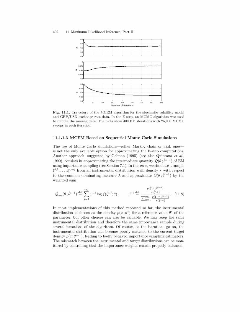
402 11 Maximum Likelihood Inference, Part II

0.4

0.5

0.6

0.7

0.8

β0.9

0.925

0.95

0.975

1

φ

0 50 100 150 200 250 300 350 400 0.1

0.15

0.2

0.25

0.3

σ

Number of Iterations

Fig. 11.1. Trajectory of the MCEM algorithm for the stochastic volatility modeland GBP/USD exchange rate data. In the E-step, an MCMC algorithm was usedto impute the missing data. The plots show 400 EM iterations with 25,000 MCMCsweeps in each iteration.

11.1.1.3 MCEM Based on Sequential Monte Carlo Simulations

The use of Monte Carlo simulations—either Markov chain or i.i.d. ones—is not the only available option for approximating the E-step computations.Another approach, suggested by Gelman (1995) (see also Quintana et al.,1999), consists in approximating the intermediate quantity Q(θ ; θi−1) of EMusing importance sampling (see Section 7.1). In this case, we simulate a sampleξi,1, . . . , ξi,mi from an instrumental distribution with density r with respectto the common dominating measure λ and approximate Q(θ ; θi−1) by theweighted sum

Qmi(θ ; θi−1) def=mi∑j=1

ωi,j log f(ξi,j ; θ) , ωi,jdef=

p(ξi,j ;θi−1)

r(ξi,j)∑mik=1

p(ξi,k ;θi−1)

r(ξi,k)

. (11.8)

In most implementations of this method reported so far, the instrumentaldistribution is chosen as the density p(x ; θ?) for a reference value θ? of theparameter, but other choices can also be valuable. We may keep the sameinstrumental distribution and therefore the same importance sample duringseveral iterations of the algorithm. Of course, as the iterations go on, theinstrumental distribution can become poorly matched to the current targetdensity p(x; θi−1), leading to badly behaved importance sampling estimators.The mismatch between the instrumental and target distributions can be mon-itored by controlling that the importance weights remain properly balanced.

11.1 Methods and Algorithms 403

For HMMs, importance sampling is seldom a sensible choice unless thenumber of observations is small (see Section 7.3.1). Natural candidates inthis context are the sequential Monte Carlo methods based on resamplingideas discussed in Chapters 7 and 8. In Section 8.3, we considered the generalproblem of estimating quantities of the form E(tn(X0:n)|Y0:n ; θ), when thefunction tn complies with Definition 4.1.2, based on sequential Monte Carlosimulations. As discussed in Section 10.2.2, the intermediate quantity of EM isprecisely of this form with an additive structure given by (10.26). Recall thatthe same remark also holds for the gradient of the log-likelihood with respectto the parameter vector θ (Section 10.2.3). For both of these, an approximationof the smoothed expectation can be computed recursively and without storingthe complete particle trajectories (see Section 8.3).

For the model of Example 11.1.2, the function tn is fully determined by thefour statistics defined in (11.4). Recursive particle smoothing for the statis-tics S0, S1, and S3 has already been considered in Example 8.3.1 (see Fig-ures 8.5 and 8.7). The case of the remaining two statistics is entirely sim-ilar. Recall from Example 8.3.1 that it is indeed possible to robustify theestimation of such smoothed sum functionals by using fixed-lag approxima-tions. The simple method proposed in Example 8.3.1 consists in replacing thesmoothing distributions φl|n by the fixed lag-smoothing distribution φl|l+k∧nfor a suitably chosen value of the delay k. The particle approximation to∑nl=0

∫s(x)lφl|l+k∧n(dxl) can be computed recursively using an algorithm

that is only marginally more complex than that used for∑nl=0

∫s(x)lφl|n(dxl).

Results obtained following this approach will be discussed in Example 11.1.3below.

11.1.2 Simulation Schedules

Although the MCEM algorithm provides a solution to intractable E-step, italso raises difficult implementation issues. Intelligent usage of the Monte Carlosimulations is necessary because MCEM can place a huge burden on the user’scomputational resources.

Heuristically there is no need to use a large number of simulations dur-ing the initial stage of the optimization. Even rather crude estimation ofQ(θ ; θi−1) might suffice to drive the parameters toward the region of interest.As the EM iterations go on, the number of simulations should be increasedhowever to avoid “zig-zagging” when the algorithm approaches convergence.Thus, in making the trade-off between improving accuracy and reducing thecomputational cost associated with a large sample size, one should favor in-creasing the sample size mi as θi approaches its limit. Determining exactlyhow this increase should be accomplished to produce the “best” possible re-sult is a topic that still attracts much research interest (Booth and Hobert,1999; Levine and Casella, 2001; Levine and Fan, 2004).

Example 11.1.3 (MCEM with Increasing Simulation Schedule). Re-sults comparable to those of the “brute force” version of the MCEM algorithm

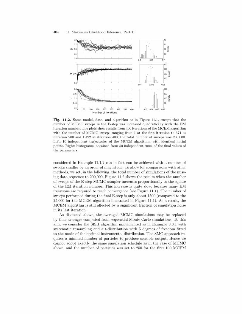
404 11 Maximum Likelihood Inference, Part II

0.4

0.5

0.6

0.7

0.8

β

0.6 0.65 0.7

10

20

30

40

Den

sity

0.9

0.95

1

φ

0.97 0.975 0.98

100

200

300

400

Den

sity

0 50 100 150 200 250 300 350 4000.1

0.15

0.2

0.25

0.3

σ

Number of Iterations0.15 0.16 0.17 0.18

50

100

150

200

Den

sity

Fig. 11.2. Same model, data, and algorithm as in Figure 11.1, except that thenumber of MCMC sweeps in the E-step was increased quadratically with the EMiteration number. The plots show results from 400 iterations of the MCEM algorithmwith the number of MCMC sweeps ranging from 1 at the first iteration to 374 atiteration 200 and 1,492 at iteration 400; the total number of sweeps was 200,000.Left: 10 independent trajectories of the MCEM algorithm, with identical initialpoints. Right: histograms, obtained from 50 independent runs, of the final values ofthe parameters.

considered in Example 11.1.2 can in fact can be achieved with a number ofsweeps smaller by an order of magnitude. To allow for comparisons with othermethods, we set, in the following, the total number of simulations of the miss-ing data sequence to 200,000. Figure 11.2 shows the results when the numberof sweeps of the E-step MCMC sampler increases proportionally to the squareof the EM iteration number. This increase is quite slow, because many EMiterations are required to reach convergence (see Figure 11.1). The number ofsweeps performed during the final E-step is only about 1500 (compared to the25,000 for the MCEM algorithm illustrated in Figure 11.1). As a result, theMCEM algorithm is still affected by a significant fraction of simulation noisein its last iteration.

As discussed above, the averaged MCMC simulations may be replacedby time-averages computed from sequential Monte Carlo simulations. To thisaim, we consider the SISR algorithm implemented as in Example 8.3.1 withsystematic resampling and a t-distribution with 5 degrees of freedom fittedto the mode of the optimal instrumental distribution. The SMC approach re-quires a minimal number of particles to produce sensible output. Hence wecannot adopt exactly the same simulation schedule as in the case of MCMCabove, and the number of particles was set to 250 for the first 100 MCEM

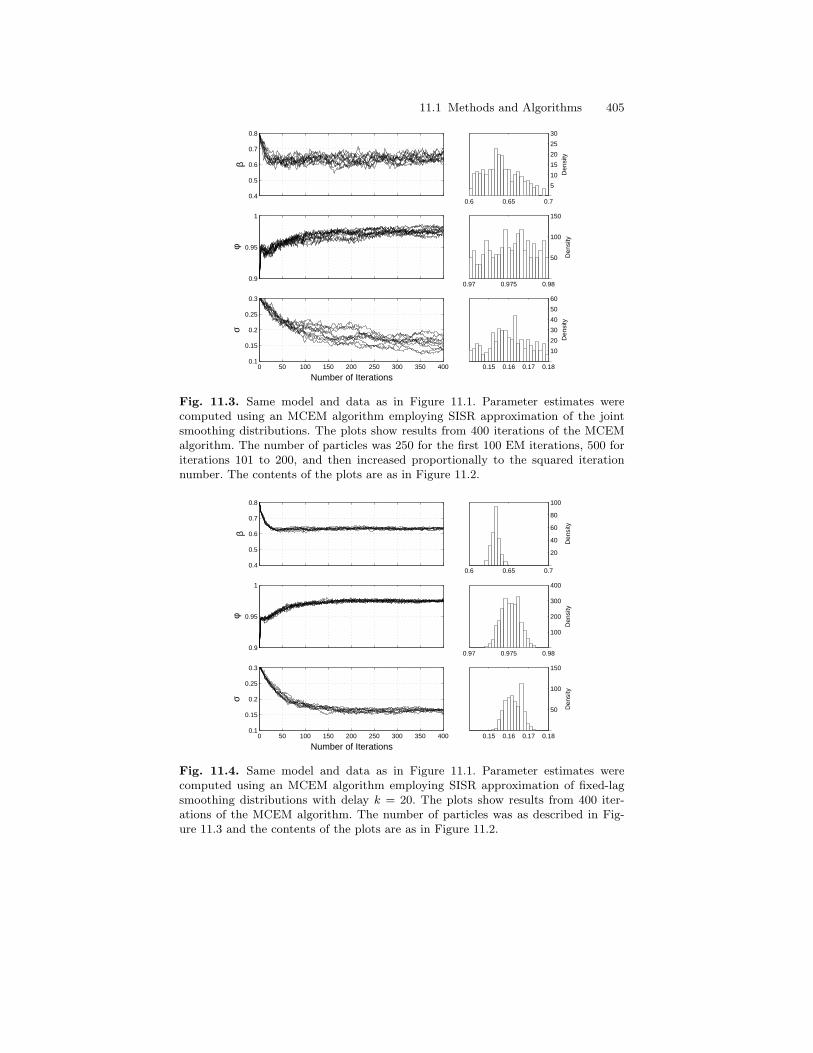
11.1 Methods and Algorithms 405

0.4

0.5

0.6

0.7

0.8

β

0.6 0.65 0.7

5

10

15

20

25

30

Den

sity

0.9

0.95

1

φ

0.97 0.975 0.98

50

100

150

Den

sity

0 50 100 150 200 250 300 350 4000.1

0.15

0.2

0.25

0.3

σ

Number of Iterations0.15 0.16 0.17 0.18

10

20

30

40

50

60

Den

sity

Fig. 11.3. Same model and data as in Figure 11.1. Parameter estimates werecomputed using an MCEM algorithm employing SISR approximation of the jointsmoothing distributions. The plots show results from 400 iterations of the MCEMalgorithm. The number of particles was 250 for the first 100 EM iterations, 500 foriterations 101 to 200, and then increased proportionally to the squared iterationnumber. The contents of the plots are as in Figure 11.2.

0.4

0.5

0.6

0.7

0.8

β

0.6 0.65 0.7

20

40

60

80

100

Den

sity

0.9

0.95

1

φ

0.97 0.975 0.98

100

200

300

400

Den

sity

0 50 100 150 200 250 300 350 4000.1

0.15

0.2

0.25

0.3

σ

Number of Iterations0.15 0.16 0.17 0.18

50

100

150

Den

sity

Fig. 11.4. Same model and data as in Figure 11.1. Parameter estimates werecomputed using an MCEM algorithm employing SISR approximation of fixed-lagsmoothing distributions with delay k = 20. The plots show results from 400 iter-ations of the MCEM algorithm. The number of particles was as described in Fig-ure 11.3 and the contents of the plots are as in Figure 11.2.

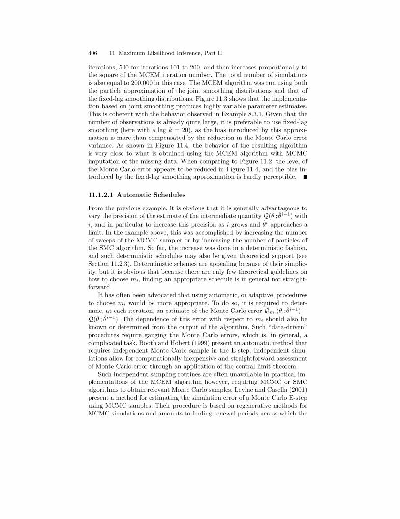
406 11 Maximum Likelihood Inference, Part II

iterations, 500 for iterations 101 to 200, and then increases proportionally tothe square of the MCEM iteration number. The total number of simulationsis also equal to 200,000 in this case. The MCEM algorithm was run using boththe particle approximation of the joint smoothing distributions and that ofthe fixed-lag smoothing distributions. Figure 11.3 shows that the implementa-tion based on joint smoothing produces highly variable parameter estimates.This is coherent with the behavior observed in Example 8.3.1. Given that thenumber of observations is already quite large, it is preferable to use fixed-lagsmoothing (here with a lag k = 20), as the bias introduced by this approxi-mation is more than compensated by the reduction in the Monte Carlo errorvariance. As shown in Figure 11.4, the behavior of the resulting algorithmis very close to what is obtained using the MCEM algorithm with MCMCimputation of the missing data. When comparing to Figure 11.2, the level ofthe Monte Carlo error appears to be reduced in Figure 11.4, and the bias in-troduced by the fixed-lag smoothing approximation is hardly perceptible.

11.1.2.1 Automatic Schedules

From the previous example, it is obvious that it is generally advantageous tovary the precision of the estimate of the intermediate quantity Q(θ ; θi−1) withi, and in particular to increase this precision as i grows and θi approaches alimit. In the example above, this was accomplished by increasing the numberof sweeps of the MCMC sampler or by increasing the number of particles ofthe SMC algorithm. So far, the increase was done in a deterministic fashion,and such deterministic schedules may also be given theoretical support (seeSection 11.2.3). Deterministic schemes are appealing because of their simplic-ity, but it is obvious that because there are only few theoretical guidelines onhow to choose mi, finding an appropriate schedule is in general not straight-forward.

It has often been advocated that using automatic, or adaptive, proceduresto choose mi would be more appropriate. To do so, it is required to deter-mine, at each iteration, an estimate of the Monte Carlo error Qmi(θ ; θi−1)−Q(θ ; θi−1). The dependence of this error with respect to mi should also beknown or determined from the output of the algorithm. Such “data-driven”procedures require gauging the Monte Carlo errors, which is, in general, acomplicated task. Booth and Hobert (1999) present an automatic method thatrequires independent Monte Carlo sample in the E-step. Independent simu-lations allow for computationally inexpensive and straightforward assessmentof Monte Carlo error through an application of the central limit theorem.

Such independent sampling routines are often unavailable in practical im-plementations of the MCEM algorithm however, requiring MCMC or SMCalgorithms to obtain relevant Monte Carlo samples. Levine and Casella (2001)present a method for estimating the simulation error of a Monte Carlo E-stepusing MCMC samples. Their procedure is based on regenerative methods forMCMC simulations and amounts to finding renewal periods across which the

11.1 Methods and Algorithms 407

MCMC trajectories are independent (see for instance Hobert et al., 2002). Bysubsampling the chain between regeneration times, Monte Carlo error may beassessed through the CLT for independent outcomes in a manner analogousto Booth and Hobert (1999). For phi-irreducible Markov chains, such renewalperiods can be obtained using the splitting procedure, which requires deter-mining small sets (see Section 14.2 for definitions of the concepts mentionedhere). A drawback of this approach is that it may be difficult, if not impos-sible, to establish the minorization condition necessary for implementing theregenerative simulation procedure. Once such a minorization condition hasbeen established however, implementing the procedure is nearly trivial.

Both of the automatic procedures mentioned above are able to decidewhen to increase the Monte Carlo sample size, but the choice of sample sizeat each such instance is arbitrary. Levine and Fan (2004) present a methodthat overcomes the limitations of the previous algorithm. The Monte Carloerror is gauged directly using a subsampling technique, and the authors useasymptotic results to construct an adaptive rule for updating the Monte Carlosample size.

Despite their obvious appeal, automatic methods suffer from some draw-backs. First, the estimation of the Monte Carlo error induces a computationaloverhead that might be non-negligible. Second, because the number of simu-lations at each iteration is random, the total amount of computation cannotbe fixed beforehand; this may be inconvenient. Finally, the convergence ofthe proposed schemes are based on heuristic arguments and have not beenestablished on firm grounds.

11.1.2.2 Averaging

There is an alternative to automatic selection of the Monte Carlo sample size,developed by Fort and Moulines (2003), which is straightforward to implementand most often useful. This method is inspired by the averaging procedureoriginally proposed by Polyak (1990) to improve the rate of convergence ofstochastic approximation procedures.

To motivate the construction of the averaging procedure, note that pro-vided that the sequence θi converges to a limit θ?, each value of θi may itselfbe considered as an estimator of the associated limit θ?. Theorem 11.2.14 as-serts that the variance of θi − θ? is of order 1/mi. Thus, in the idealizedsituation where the random perturbations θi− θ? would also be uncorrelated,it is well-known that it is possible to obtain an improved estimator of θ? bycombining the individual estimates θi in proportion of the inverse of theirvariance (this is the minimum variance estimate of θ?). This optimal linearcombination has a variance that decreases as 1/

∑imi, that is, the total num-

ber of simulations rather than the final number of simulations. Although theMCEM perturbations θi − θ? are not uncorrelated, even when using i.i.d.Monte Carlo simulation, due to the dependence with respect to θ, Fort andMoulines (2003) suggested using the averaged MCEM estimator

408 11 Maximum Likelihood Inference, Part II

θidef=

i∑j=i0

mj∑ij=i0

mj

θj , for i ≥ i0, (11.9)

where i0 is the iteration index at which computation of the average is started.In general, it is not recommended to start averaging too early, when thealgorithm is still in its transient phase.

Example 11.1.4 (Averaging). In Example 11.1.3, the number of sweeps isincreased quite slowly and the number of sweeps during the final EM iter-ations is not large (about 1500). This scheme is advantageous in situationswhen the EM algorithm is slow, because a large number of iterations can beperformed while keeping the total of number of simulations moderate. Theproblem is rather that the simulation noise at convergence is still significant(see Figure 11.2). This is a typical situation in which averaging can prove tobe very helpful. As seen in Figure 11.5, averaging reduces the noise when theparameters are in the neighborhood of their limits. Averaging is also benefi-cial when the EM statistics are estimated using sequential Monte Carlo (seeFigure 11.6).

11.1.3 Gradient-based Algorithms

As discussed in Section 10.2.3, computation of the gradient of the log-likelihood is very much related to the E-step of EM as a consequence of Fisher’sidentity (Proposition 10.1.6). It is thus rather straightforward to derive MonteCarlo versions of the gradient algorithms introduced in Section 10.1.3. Atthe ith iteration, one may for example approximate the gradient of the log-likelihood ∇θ`(θi−1), where θi−1 denotes the current parameter estimate, by

∇θ`mi(θi−1) =

1mi

mi∑j=1

∇θ log f(ξi,j ; θi−1) , (11.10)

where ξi,1, . . . , ξi,mi is an i.i.d. sample from the density p(x ; θi−1) or a re-alization of an ergodic Markov chain admitting p(x ; θi−1) as its stationarydensity. It is also possible to use importance sampling; if ξi,1, . . . , ξi,mi is asample from the instrumental distribution r, then the IS estimate of∇θ`(θi−1)is

∇θ`m(θi−1) =mi∑j=1

ωi,j∇θ log f(ξi,j ; θi−1), ωi,j =

p(ξi,j ;θi−1)

r(ξi,j)∑mik=1

p(ξi,k;θi−1)

r(ξi,k)

(11.11)As in the case of MCEM, it is likely that for HMMs, importance samplingstrategies become unreliable when the number of observations increases. Tocircumvent the problem, one may use sequential Monte Carlo methods such

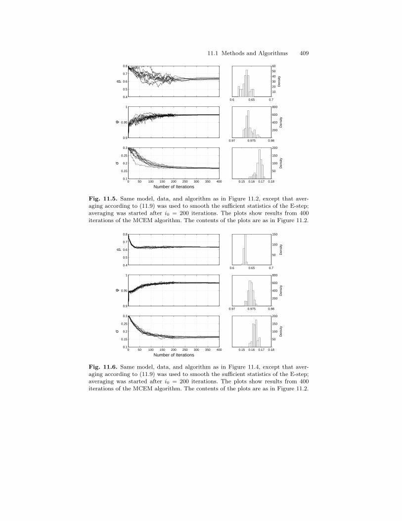
11.1 Methods and Algorithms 409

0.4

0.5

0.6

0.7

0.8

β

0.6 0.65 0.7

10

20

30

40

50

60

Den

sity

0.9

0.95

1

φ

0.97 0.975 0.98

200

400

600

800

Den

sity

0 50 100 150 200 250 300 350 4000.1

0.15

0.2

0.25

0.3

σ

Number of Iterations0.15 0.16 0.17 0.18

50

100

150

200

Den

sity

Fig. 11.5. Same model, data, and algorithm as in Figure 11.2, except that aver-aging according to (11.9) was used to smooth the sufficient statistics of the E-step;averaging was started after i0 = 200 iterations. The plots show results from 400iterations of the MCEM algorithm. The contents of the plots are as in Figure 11.2.

0.4

0.5

0.6

0.7

0.8

β

0.6 0.65 0.7

50

100

150

Den

sity

0.9

0.95

1

φ

0.97 0.975 0.98

200

400

600

800

Den

sity

0 50 100 150 200 250 300 350 4000.1

0.15

0.2

0.25

0.3

σ

Number of Iterations0.15 0.16 0.17 0.18

50

100

150

200

Den

sity

Fig. 11.6. Same model, data, and algorithm as in Figure 11.4, except that aver-aging according to (11.9) was used to smooth the sufficient statistics of the E-step;averaging was started after i0 = 200 iterations. The plots show results from 400iterations of the MCEM algorithm. The contents of the plots are as in Figure 11.2.

410 11 Maximum Likelihood Inference, Part II

as SISR where (11.11) is not computed directly but rather constructed re-cursively (in time) following the approach discussed in Section 8.3 and usedin the case of MCEM above. Details are omitted because the gradient of thelog-likelihood (10.29) and the intermediate quantity of EM (10.26) are verysimilar. For models that belong to exponential families, the only quantitiesthat need to be computed in both cases are the smoothed expectation of thesufficient statistics, and hence both computations are exactly equivalent.

Louis’s identity (see Proposition 10.1.6) suggests an approximation of theHessian of `(θ) at θi−1 of the form

Jmi(θi−1) =

1mi

mi∑j=1

∇2θ log f(ξi,j ; θi−1) +

1mi

mi∑j=1

[∇θ log f(ξi,j ; θi−1)

]⊗2

−[∇θ`mi(θ

i−1)]⊗2

,

where ξi,1, . . . , ξi,mi are as above, for a vector a we have used the notationa⊗2 = aat, and the estimate of the gradient in the final term on the right-hand side may be chosen, for instance, as in (11.10). Using this approxima-tion of the Hessian, it is possible to formulate a Monte Carlo version of theNewton-Raphson procedure. This algorithm was first proposed by Geyer andThompson (1992) in an exponential family setting and then generalized byGelfand and Carlin (1993). Gelman (1995) proposed a similar algorithm inwhich importance sampling is used as the Monte Carlo method.

Now assume that we have, with the help of a Monte Carlo approximationof the gradient and possibly also the Hessian, selected a search direction. Thenext step is then to determine an appropriate value of the step size γ (seeSection 10.1.3). This is not a simple task, because the objective function `(θ)cannot be evaluated analytically, and therefore it is not possible to implementa line search—at least not in an immediate way. A simple option consists inusing a step size that is small but fixed (see Dupuis and Simha, 1991), and tolet mi →∞ as sufficiently fast as i→∞.

If we want to optimize the step size, we have to approximate the objec-tive function in the search direction. We may for example follow the methodproposed by Geyer and Thompson (1992), which consists in approximating(locally) the ratio L(θ)/L(θi−1) by

mi∑j=1

f(ξi,j ; θ)

f(ξi,j ; θi−1),

where ξi,j are the samples from p(x ; θi−1) used to determine the searchdirection. Under standard assumptions, the sum of this display converges inprobability as mi →∞ to∫

f(x ; θ)

f(x ; θi−1)p(x ; θi)λ(dx) =

L(θ)

L(θi−1).

11.1 Methods and Algorithms 411

This suggests approximating the difference `(θ) − `(θi−1) in a neighborhoodof θi−1 by

log

1mi

mi∑j=1

f(ξi,j ; θ)

f(ξi,j ; θi−1)

. (11.12)

This type of approximation nevertheless needs to be considered with somecare because the search direction is not necessarily an ascent direction for thisapproximation of the objective function due to the Monte Carlo errors. To thebest of our knowledge, this type of approximation has not been thoroughlyinvestigated in practice.

As for the MCEM algorithm, it is not necessary to estimate the objectivefunction and its gradient with high accuracy during the initial optimizationsteps. Therefore, the Monte Carlo sample sizes should not be taken large atthe beginning of the procedure but should be increased when the algorithmapproaches convergence. Procedures to adapt the sample size mi at each it-eration are discussed and analyzed by Sakalauskas (2000, 2002) for gradientalgorithms using a (small enough) fixed step size. The suggestion of this au-thor is to increase mi proportionally to the inverse of the squared norm of the(estimated) gradient at the current parameter estimate. If this proportional-ity factor is carefully adjusted, it may be shown, under a set of restrictiveconditions, that the Monte Carlo steepest ascent algorithm converges almostsurely to a stationary point of the objective function.

It is fair to say that in the case of general state space HMMs, gradient-based methods as less popular than their counterparts based on the EMparadigm. An important advantage of EM based methods in this contextis that they are parameterization independent (see Section 10.1.4 for furtherdiscussion). This property means that the issue of selecting a proper step sizeγ—which is problematic in simulation-based approaches as discussed above—has no counterpart for EM-based methods, which are scale-free. Rememberthat it is also precisely the reason why the EM approach sometimes convergesmuch more slowly than gradient-based methods.

11.1.4 Interlude: Stochastic Approximation and theRobbins-Monro Approach

Stochastic approximation is a general term for methods that recursively searchfor an optimum or zero of a function that can only be observed disturbedby some noise. The original work in the stochastic approximation literaturewas by Robbins and Monro (1951), who developed and analyzed a recursiveprocedure for finding the root(s) of the equation h(θ) = 0. If the function hwas known, a simple procedure to find a root consists in using the elementaryalgorithm

θi = θi−1 + γih(θi−1) , (11.13)

412 11 Maximum Likelihood Inference, Part II

where γi is a sequence of positive step sizes. In many applications, theevaluation of h(θ) cannot be performed, either because it is computationallyprohibitive or analytical formulas are simply not available, but noise-corruptedobservations of the function can be obtained for any value of the parameterθ ∈ Θ ⊆ Rdθ . One could then, for instance, consider using the procedure(11.13) but with h(θ) replaced by an accurate estimate of its value obtainedby averaging many noisy observations of the function.

It was recognized by Robbins and Monro (1951) that averaging a largenumber of observations of the function at θi−1 is not always the most efficientsolution. Indeed, the value of the function h(θi−1) is only of interest in so farthat it leads us in the right direction, and it is not unreasonable to expectthat this happens, at least on the average, even if the estimate is not veryaccurate. Robbins and Monro (1951) rather proposed the algorithm

θi = θi−1 + γiYi , (11.14)

where γi is a deterministic sequence satisfying

γi > 0, limi→∞

γi = 0,∑i

γi =∞ ,

and Y i is a noisy observation of h(θi−1). Although the analysis of the methodis certainly simpler when the noise sequence Y i−h(θi−1)i≥1 is i.i.d., in manypractical applications the noise Y i − h(θi−1) depends on θi−1 and sometimeson past values of θj and Y j , for j ≤ i− 1 (see for instance Benveniste et al.,1990; Kushner and Yin, 2003). Using a decreasing step size implies that theparameter sequence θi moves slower as i goes to infinity; the basic idea isthat decreasing step sizes provides an averaging of the random errors com-mitted when evaluating the function h.

Ever since the introduction of the now classic Robbins-Monro algorithm,stochastic approximation has been successfully used in many applications andhas received wide attention in the literature. The convergence of the stochas-tic approximation scheme is also a question of importance that has been ad-dressed under a variety of conditions, which cover most of the applications (seefor instance Benveniste et al., 1990; Duflo, 1997; Kushner and Yin, 2003).

11.1.5 Stochastic Gradient Algorithms

We now come back to the generic incomplete data model, considering severalways in which the stochastic approximation approach may be put in use. Thefirst obvious option is to apply the Robbins-Monro algorithm to determinethe roots of the equations ∇θ`(θ) = 0, yielding the following recursions

θi = θi−1 + γi∇θ log f(ξi ; θi−1) , (11.15)

where ξi is a sample from the density p(x ; θi−1). That is, defining the filtrationF i such that F i−1 = σ(θ0, ξ0, . . . , ξi−1),

11.1 Methods and Algorithms 413

ξi | F i−1 ∼ p(·; θi−1) .

Thus Y i = ∇θ log f(ξi ; θi−1) can be considered as a noisy measurement of∇θ`(θi−1) because of the Fisher identity, E[Y i | F i−1] = ∇θ`(θi−1). Hence wecan write Y i = ∇θ`(θi−1) + ζi, with

ζi = ∇θ log f(ξi ; θi−1)− E[∇θ log f(ξi) ; θi−1 | F i−1] ;

obviously ζi is an F i-adapted martingale difference sequence.Often it is not possible to sample directly from the density p(x ; θi−1).

One can then replace this draw by iterations from a Markov chain admittingp(x ; θi−1) as its stationary density. Then E[Y i | F i−1] does no longer equal∇θ`(θi−1), but rather

ξi | F i−1 ∼ Πθi−1(ξi−1, ·) , (11.16)

where for any θ ∈ Θ, Πθ is a transition kernel of an ergodic Markov chainwith stationary density p(x ; θ). Such algorithms were considered by Younes(1988, 1989) for maximum likelihood estimation in partially observed Gibbsfields. They were later extended by Gu and Kong (1998) to maximum likeli-hood estimation in general incomplete data problems by (see also Gu and Li,1998; Delyon et al., 1999, Section 8). In this case, the noise structure is morecomplicated and analysis and control of the convergence of such algorithmsbecome intricate (see Andrieu et al., 2005, for results in this direction).

Several improvements can be brought to this scheme. First, it is sometimesrecommendable to run a certain number, saym, of simulations before updatingthe value of the parameter. That is,

θi = θi−1 + γi

1m

m∑j=1

∇θ log f(ξi,j ; θi−1)

, (11.17)

where ξi,1, . . . , ξi,m are draws from p(x ; θi−1). Choosing m > 1 is generallybeneficial in that it makes the procedure more stable and saves computationaltime. The downside is that there are few theoretical guidelines on how to setthis number. The above algorithm is very close to the Monte Carlo versionof the steepest ascent method. Another possible improvement, much in thespirit of quasi-Newton algorithms, is to modify the search direction by letting

θi = θi−1 + γiWi

1m

m∑j=1

∇θ log f(ξi,j ; θi−1)

, (11.18)

where W i is a properly chosen weight matrix (see for instance Gu and Li,1998; Gu and Kong, 1998).

One of the main appeals of stochastic approximation is that, at least inprinciple, the only decision that has to be made is the choice of the step size

414 11 Maximum Likelihood Inference, Part II

schedule. Although in theory the method converges for a wide variety of stepsizes (see Section 11.3), in practice the choice of step sizes influences the actualnumber of simulations needed to take the parameter estimate into the neigh-borhood of the solution (transient regime) and its fluctuations around the so-lution (misadjustment near convergence). Large step sizes generally speed upconvergence to a neighborhood of the solution but fail to mitigate simulationnoise. Small step sizes reduce noise but cause slow convergence. Heuristically,it is appropriate to use large step sizes until the algorithm reaches a neighbor-hood of the solution and then to switch to smaller step sizes (see for instanceGu and Zhu, 2001, for applications to the stochastic gradient algorithm).

A way to alleviate the step size selection problem is to use averaging asin Section 11.1.2. Polyak (1990) (see also Polyak and Juditsky, 1992) showedthat if the sequence of step sizes γi tends to zero slower than 1/i, yet fastenough to ensure convergence at a given rate, then the running average

θidef= (i− i0 + 1)−1

i∑j=i0

θj , i ≥ i0 , (11.19)

converges at an optimal rate. Here i0 is an index at which averaging starts,so as to discard the very first steps. This result implies that one should adoptstep sizes larger than usual but in conjunction with averaging (to control theincreased noise due to use of the larger step sizes). The practical value ofaveraging has been reported in many different contexts—see (Kushner andYin, 2003, Chapter 11) for a thorough investigation averaging, as well as(Delyon et al., 1999).

11.1.6 Stochastic Approximation EM

We now consider a variant of the MCEM algorithm that may also be inter-preted as a stochastic approximation procedure. Compared to the stochasticgradient approach discussed in the previous section, this algorithm is scale-freein the sense that the step sizes are positive numbers restricted to the inter-val [0, 1]. Compared to the MCEM approach, the E-step involves a weightedaverage of the approximations of the intermediate quantity of EM obtainedin the current as well as in the previous iterations. Hence there is no need toincrease the number of replications of the missing data as in MCEM.

Algorithm 11.1.5 (Stochastic Approximation EM). Given an initial pa-

rameter estimate θ0 and a decreasing sequence of positive step sizes γii≥1 suchthat γ1 = 1, do, for i = 1, 2 . . . ,

Simulation: Draw ξi,1, . . . , ξi,m from the conditional density p(x ; θi−1).

Maximization: Compute θi as the maximum of the function Qi(θ) over the feasibleset Θ, where

11.1 Methods and Algorithms 415

Qi(θ) = Qi−1(θ) + γi

1m

m∑j=1

log f(ξi,j ; θ)− Qi−1(θ)

. (11.20)

This algorithm, called the stochastic approximation EM (SAEM) algorithm,was proposed by Cardoso et al. (1995) and further analyzed by Delyon et al.(1999) and Kuhn and Lavielle (2004). To understand why this algorithm canbe cast into the Robbins-Monro framework, consider the simple case wherethe complete data likelihood is from an exponential family of distributions.In this case, the SAEM algorithm consists in updating, at each iteration, thecurrent estimates (Si, θi) of the complete data sufficient statistic and of theparameter. Each iteration of the algorithm is divided into two steps. In a firststep, we draw ξi,1, . . . , ξi,m from the conditional density p(x ; θi−1) and updateSi according to

Si = Si−1 + γi

1m

m∑j=1

S(ξi,j)− Si−1

. (11.21)

In a second step, we compute θi as the maximum of the function ψt(θ)Si−c(θ).Assume that the function ψt(θ)s − c(θ) has a single global maximum,

denoted θ(s) for all feasible values of Si. The difference m−1∑mj=1 S(ξi,j) −

Si−1 can then be considered as a noisy observation of a function h(Si−1),where

h(s) =∫S(x)p(x ; θ(s))λ(dx)− s . (11.22)

Thus (11.21) fits into the Robbins-Monro when considering the sufficientstatistic s rather than the associated parameter θ(s). This Robbins-Monroprocedure searches for the roots of h(s) = 0, that is, the values of s satisfying∫

S(x)p(x ; θ(s))λ(dx) = s .

Assume that this equation has a solution s? and put θ? = θ(s?). Now notethat

Q(θ ; θ?) = ψt(θ)∫S(x)p(x ; θ?)λ(dx)− c(θ) = ψt(θ)s? − c(θ) ,

and by definition the maximum of the right-hand side of this display is ob-tained at θ?. Therefore, an iteration of the EM algorithm started at θ? willstay at θ?, and we find that each root s? is associated to a fixed point θ? ofthe EM algorithm.

The SAEM algorithm is simple to implement and has proved to be rea-sonably successful in different applications. Compared to the stochastic gradi-ent procedure, SAEM inherits from the expectation-maximization algorithm

416 11 Maximum Likelihood Inference, Part II

most of the properties that made the success of the EM approach (for in-stance, the simplicity with which it deals with parameter constraints). Oneof these properties is invariance with respect to the parameterization. Withthe SAEM algorithm, the scale of the step sizes γi is fixed irrespectivelyof the parameterization as γ1 equals 1. As in the case of the stochastic gra-dient, however, the rate of decrease of the step sizes strongly influences thepractical performance of the algorithm. In particular, if the convergence rateof the EM algorithm is already slow, it is unwise to choose fast decreasingstep sizes, thereby even further slowing down the method. In contrast, if EMconverges fast, then large step sizes introduce an unnecessary amount of extranoise, which should be avoided. Here again, the use of averaging is helpful inreducing the impact of the choice of the rate of decrease of the step sizes.

Example 11.1.6. We implemented the SAEM algorithm for the stochasticvolatility model and data described in Example 11.1.2, and the results aredisplayed in Figure 11.7. In each iteration of the algorithm, a single realiza-tion of the missing data was obtained using a sweep of the Gibbs sampler.This draw was used to update the stochastic approximation estimate of thecomplete data sufficient statistics, which were then used to update the pa-rameter estimate. The only tuning parameter is the sequence of step size γn.Here again the theory of stochastic approximation does not tell much aboutthe “optimal” way to choose this sequence. In view of the above discussion,we used slowly decreasing step sizes (γn = n−0.6) to speed up convergence to-ward the region of interest. As seen in Figure 11.7, the parameters estimatesobtained using this implementation of SAEM are rather noisy. In order toreduce the fluctuations, we performed averaging, computing

θi = (i− i0 + 1)−1i∑

j=i0

θi , i ≥ i0 , (11.23)

where i0 was set to 100,000. Averaging is useful only when the parameterapproaches convergence and should be turned off during the initial steps ofthe algorithm. Figure 11.8 shows results for the SAEM algorithm with aver-aging. Figures 11.7 and 11.8 should be compared with Figures 11.2 and 11.5,respectively, which involve the same sampler and the same overall number ofsimulations but were obtained using the MCEM strategy. Both procedures(SAEM and MCEM) provides comparable results.

11.1.7 Stochastic EM

The stochastic EM (SEM) algorithm is a method that shares many similar-ities with the stochastic approximation EM algorithm. The SEM algorithmwas initially proposed as a means to estimate parameters of mixtures dis-tributions (Celeux and Diebolt, 1985, 1990), but the concept can easily begeneralized to cover more general incomplete data models. The basic idea is

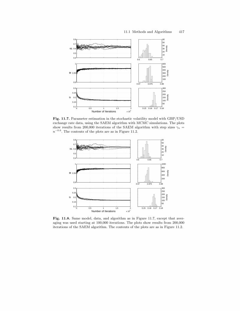
11.1 Methods and Algorithms 417

0.4

0.5

0.6

0.7

0.8

β

0.6 0.65 0.7

10

20

30

40

50

60

Den

sity

0.9

0.95

1

φ

0.97 0.975 0.98

100

200

300

400

500

600

Den

sity

0 0.5 1 1.5 2

x 105

0.1

0.15

0.2

0.25

0.3

σ

Number of Iterations0.15 0.16 0.17 0.18

50

100

150

200

250

300

Den

sity

Fig. 11.7. Parameter estimation in the stochastic volatility model with GBP/USDexchange rate data, using the SAEM algorithm with MCMC simulations. The plotsshow results from 200,000 iterations of the SAEM algorithm with step sizes γn =n−0.6. The contents of the plots are as in Figure 11.2.

0.4

0.5

0.6

0.7

0.8

β

0.6 0.65 0.7

10

20

30

40

50

60

Den

sity

0.9

0.95

1

φ

0.97 0.975 0.98

200

400

600

800

1000

Den

sity

0 0.5 1 1.5 2

x 105

0.1

0.15

0.2

0.25

0.3

σ

Number of Iterations0.15 0.16 0.17 0.18

50

100

150

200

250

300

Den

sity

Fig. 11.8. Same model, data, and algorithm as in Figure 11.7, except that aver-aging was used starting at 100,000 iterations. The plots show results from 200,000iterations of the SAEM algorithm. The contents of the plots are as in Figure 11.2.

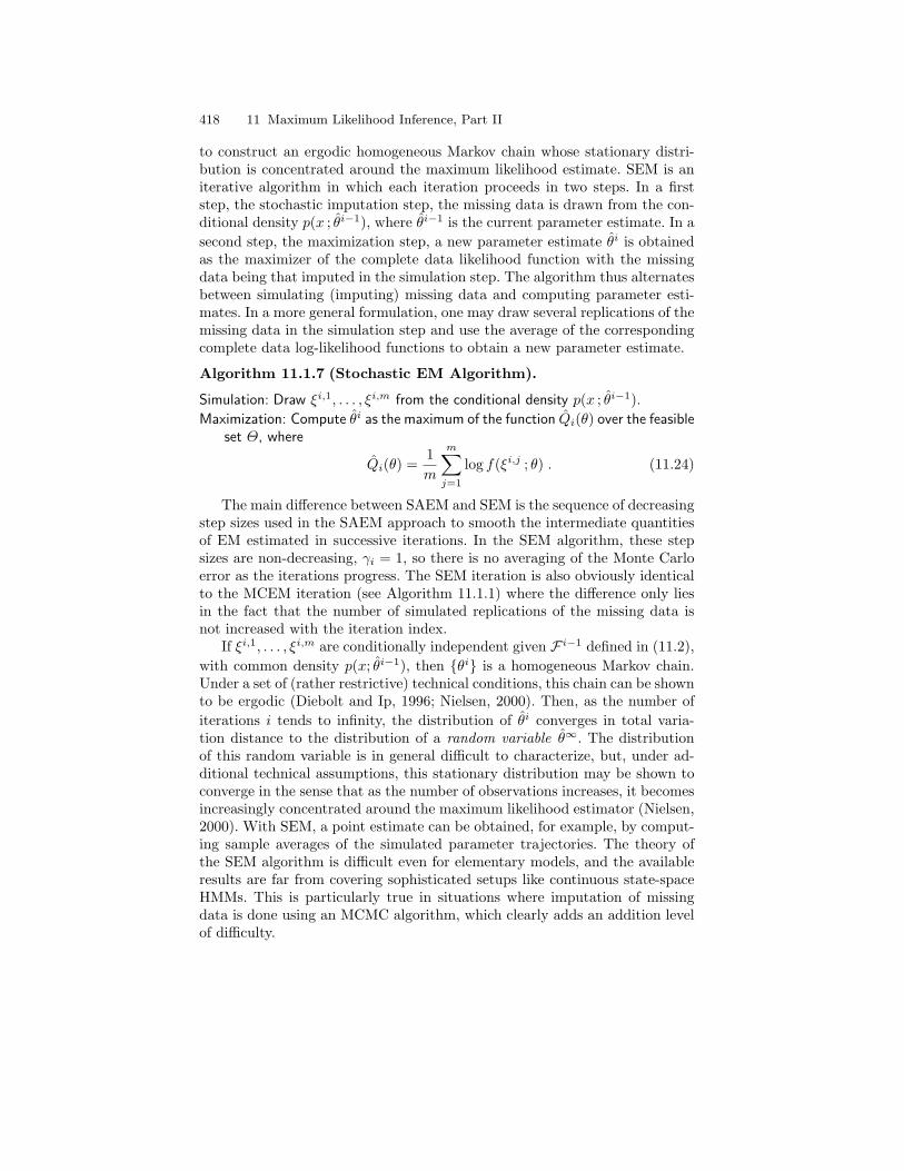
418 11 Maximum Likelihood Inference, Part II

to construct an ergodic homogeneous Markov chain whose stationary distri-bution is concentrated around the maximum likelihood estimate. SEM is aniterative algorithm in which each iteration proceeds in two steps. In a firststep, the stochastic imputation step, the missing data is drawn from the con-ditional density p(x ; θi−1), where θi−1 is the current parameter estimate. In asecond step, the maximization step, a new parameter estimate θi is obtainedas the maximizer of the complete data likelihood function with the missingdata being that imputed in the simulation step. The algorithm thus alternatesbetween simulating (imputing) missing data and computing parameter esti-mates. In a more general formulation, one may draw several replications of themissing data in the simulation step and use the average of the correspondingcomplete data log-likelihood functions to obtain a new parameter estimate.

Algorithm 11.1.7 (Stochastic EM Algorithm).

Simulation: Draw ξi,1, . . . , ξi,m from the conditional density p(x ; θi−1).

Maximization: Compute θi as the maximum of the function Qi(θ) over the feasibleset Θ, where

Qi(θ) =1m

m∑j=1

log f(ξi,j ; θ) . (11.24)

The main difference between SAEM and SEM is the sequence of decreasingstep sizes used in the SAEM approach to smooth the intermediate quantitiesof EM estimated in successive iterations. In the SEM algorithm, these stepsizes are non-decreasing, γi = 1, so there is no averaging of the Monte Carloerror as the iterations progress. The SEM iteration is also obviously identicalto the MCEM iteration (see Algorithm 11.1.1) where the difference only liesin the fact that the number of simulated replications of the missing data isnot increased with the iteration index.

If ξi,1, . . . , ξi,m are conditionally independent given F i−1 defined in (11.2),with common density p(x; θi−1), then θi is a homogeneous Markov chain.Under a set of (rather restrictive) technical conditions, this chain can be shownto be ergodic (Diebolt and Ip, 1996; Nielsen, 2000). Then, as the number ofiterations i tends to infinity, the distribution of θi converges in total varia-tion distance to the distribution of a random variable θ∞. The distributionof this random variable is in general difficult to characterize, but, under ad-ditional technical assumptions, this stationary distribution may be shown toconverge in the sense that as the number of observations increases, it becomesincreasingly concentrated around the maximum likelihood estimator (Nielsen,2000). With SEM, a point estimate can be obtained, for example, by comput-ing sample averages of the simulated parameter trajectories. The theory ofthe SEM algorithm is difficult even for elementary models, and the availableresults are far from covering sophisticated setups like continuous state-spaceHMMs. This is particularly true in situations where imputation of missingdata is done using an MCMC algorithm, which clearly adds an addition levelof difficulty.

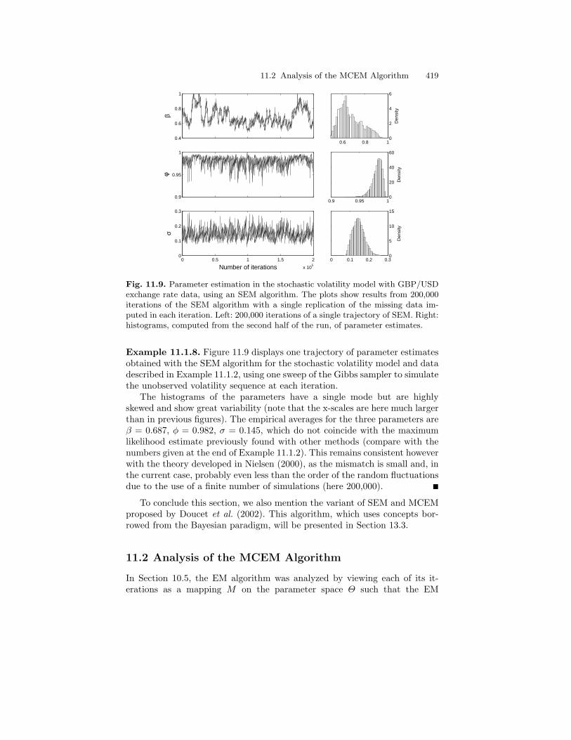
11.2 Analysis of the MCEM Algorithm 419

0.4

0.6

0.8

1

β

0.6 0.8 10

2

4

6

Den

sity

0.9

0.95

1

φ

0.9 0.95 10

20

40

60

Den

sity

0 0.5 1 1.5 2

x 105

0

0.1

0.2

0.3

σ

Number of iterations0 0.1 0.2 0.3

0

5

10

15

Den

sity

Fig. 11.9. Parameter estimation in the stochastic volatility model with GBP/USDexchange rate data, using an SEM algorithm. The plots show results from 200,000iterations of the SEM algorithm with a single replication of the missing data im-puted in each iteration. Left: 200,000 iterations of a single trajectory of SEM. Right:histograms, computed from the second half of the run, of parameter estimates.

Example 11.1.8. Figure 11.9 displays one trajectory of parameter estimatesobtained with the SEM algorithm for the stochastic volatility model and datadescribed in Example 11.1.2, using one sweep of the Gibbs sampler to simulatethe unobserved volatility sequence at each iteration.

The histograms of the parameters have a single mode but are highlyskewed and show great variability (note that the x-scales are here much largerthan in previous figures). The empirical averages for the three parameters areβ = 0.687, φ = 0.982, σ = 0.145, which do not coincide with the maximumlikelihood estimate previously found with other methods (compare with thenumbers given at the end of Example 11.1.2). This remains consistent howeverwith the theory developed in Nielsen (2000), as the mismatch is small and, inthe current case, probably even less than the order of the random fluctuationsdue to the use of a finite number of simulations (here 200,000).

To conclude this section, we also mention the variant of SEM and MCEMproposed by Doucet et al. (2002). This algorithm, which uses concepts bor-rowed from the Bayesian paradigm, will be presented in Section 13.3.

11.2 Analysis of the MCEM Algorithm

In Section 10.5, the EM algorithm was analyzed by viewing each of its it-erations as a mapping M on the parameter space Θ such that the EM

420 11 Maximum Likelihood Inference, Part II

sequence of estimates is given by the iterates θi+1 = M(θi). Under mildconditions, the EM sequence eventually converges to the set of fixed points,L = θ ∈ Θ : θ = M(θ), of this mapping. EM is an ascent algorithm as eachiteration of M increases the observed log-likelihood `, that is, ` M(θ) ≥ `(θ)for any θ ∈ Θ with equality if and only if θ ∈ L. This ascent property is essen-tial in showing that the algorithm converges: it guarantees that the sequence`(θi) is non-decreasing and, hence, convergent if it is bounded.

The MCEM algorithm is an approximation of the EM algorithm. Eachiteration of the MCEM algorithm is a perturbed version of an EM iteration,where the “typical size” of the perturbation is controlled by the Monte Carloerror and thus by the number of simulations. The MCEM sequence may thusbe written under the form θi+1 = M(θi) + ζi+1, where ζi+1 is the pertur-bation due to the Monte Carlo approximation. Provided that the number ofsimulations is increased as the algorithm approaches convergence, the pertur-bation ζi vanishes as i→∞. Note that the MCEM algorithm is not an ascentalgorithm, which prevents us from using the general convergence results ofSection 10.5. It is sensible however to expect that the behavior of the MCEMalgorithm closely follows that of the EM algorithm, at least for large i, as therandom perturbations vanish in the limit.

To prove that this intuition is correct, we first establish in Section 11.2.1a stability result for deterministically perturbed dynamical systems and thenuse this result in Section 11.2.2 to deduce a set of conditions implying almostsure convergence of the MCEM algorithm. To avoid entering into too manytechnicalities, we study convergence under elementary assumptions that donot cover all possible applications of MCEM to maximum likelihood estima-tion in partially observed models. We feel however that a first exposure tothis theory should not be obscured by too many distracting details that willalmost inevitably arise when trying to cover more sophisticated cases.

Remark 11.2.1 (Stability in Stochastic Algorithms). One topic of im-portance that we entirely avoid here is the stability issue. We always assumethat it can be independently guaranteed that the sequence of estimates pro-duced by the algorithm deterministically stays in a compact set. Althoughthis will obviously be the case where the parameter space Θ is compact, thisassumption may fail to hold in more general settings where the algorithms un-der study can generate sequences of parameters that either diverge erraticallyor converge toward the boundary of the parameter space. To circumvent thisproblem, from both practical and theoretical points of view, it is necessaryto modify the elementary recursion of the algorithm, for instance using re-projections (Kushner and Yin, 2003; Fort and Moulines, 2003; Andrieu et al.,2005).

11.2.1 Convergence of Perturbed Dynamical Systems

Let T : Θ → Θ be a (point-to-point) map on Θ. We study in this sectionthe convergence of the Θ-valued discrete time dynamical system θi+1 = T (θi)

11.2 Analysis of the MCEM Algorithm 421

and the perturbed dynamical system θi+1 = T (θi) + ζi+1, where ζi is adeterministic sequence converging to zero. The study of such perturbed dy-namical systems was initiated by Kesten (1972), and these results have laterbeen extended by Pierre-Loti-Viaud (1995), Brandiere (1998), and Bonnansand Shapiro (1998).

To study the convergence, it is useful to introduce Lyapunov functionsassociated with the mapping T . A Lyapunov function, as defined below, isequivalent to the concept of ascent function that we met in Section 10.5 whendiscussing the convergence of EM. The terminology “Lyapunov function” ishowever more standard, except in numerical optimization texts. Note thatLyapunov functions are traditionally defined as descent functions rather thanascent functions. We reverse this convention to be consistent with the factthat the MLE estimator is defined as the maximum of the (log-)likelihoodfunction.

Definition 11.2.2 (Lyapunov Function). T : Θ → Θ be a map as aboveand let

L def= θ ∈ Θ : θ = T (θ) (11.25)

be the set of fixed points of this map. A function W : Θ → R is said to be aLyapunov function relative to (T,Θ) if W is continuous and W T (θ) ≥W (θ)for all θ ∈ Θ, with equality if and only if θ ∈ L.

In other words, the map T is an ascent algorithm for the function W .

Theorem 11.2.3. Let Θ be an open subset of Rdθ and let T : Θ → Θ be acontinuous map with set L of fixed points. Assume that there exists a Lyapunovfunction W relative to (T,Θ) such that W (L) is a finite set of points. Let Kbe a compact set and θi a K-valued sequence satisfying

limi→∞

|W (θi+1)−W T (θi)| = 0 . (11.26)

Then the set L ∩ K is non-empty, the sequence W (θi) converges to a pointw? ∈W (L∩K), and the sequence θi converges to the set Lw? = θ ∈ L∩K :W (θ) = w?.

The proof of the theorem is based on the following result.

Lemma 11.2.4. Let ε > 0 be a real constant, let n ≥ 1 be an integer, and let−∞ < a1 < b1 < . . . < an < bn < ∞ be real numbers. Let wj and ej betwo sequences such that lim supj→∞ wj <∞, limj→∞ ej = 0 and

wj+1 ≥ wj + ε1Ac(wj) + ej , where Adef=

n⋃i=1

[ai, bi] . (11.27)

Then there exists an index k? ∈ 1, . . . , n such that ak? ≤ lim inf wj ≤lim supwj ≤ bk? .

422 11 Maximum Likelihood Inference, Part II

Proof. First note that (11.27) implies that the sequence wj is infinitely oftenin the set A (otherwise it would tend to infinity, contradicting the assump-tions). Thus it visits infinitely often at least one of the intervals [ak, bk] forsome k. Choose η < ε ∧ inf1≤i≤n−1(ai+1 − bi)/2 and set j0 such that |ej | ≤ ηfor j ≥ j0. Let p ≥ j0 such that wp ∈ [ak, bk]. We will show that

for any j ≥ p , wj ≥ ak − η . (11.28)

The property is obviously true for j = p. Assume now that the property holdstrue for some j ≥ p. If wj ≥ ak, then (11.27) shows that wj+1 ≥ ak − η.If ak − η ≤ wj < ak, then wj+1 ≥ wj + ε − η ≥ ak − η. Therefore wj+1 ≥ak − η, and (11.28) follows by induction. Because η was arbitrary, we findthat lim inf wj ≥ ak. Using a similar induction argument, one may show thatlim supwj ≤ bk, which concludes the proof. ut

Proof (of Theorem 11.2.3). If L ∩ K was empty, then minθ∈ KW T (θ) −W (θ) > 0, which would contradict (11.26). Hence L ∩ K is non-empty. Forsimplicity, we assume in the following that L ⊆ K, if not, simply replace L byL ∩ K.

For any α > 0, let [W (L)]αdef= x ∈ R : infy∈W (L) |x− y| < α. Because

W (L) is bounded, the set [W (L)]α is a finite union of disjoint bounded openintervals of length at least equal to 2α. Thus there exists an integer nα ≥ 0and real numbers aα(1) < bα(1) < . . . < aα(nα) < bα(nα) such that

[W (L)]α =nα⋃k=1

(aα(k), bα(k)) . (11.29)

Note that W−1([W (L)]α) is an open neighborhood of L, and define

εdef= infθ∈K\W−1([W (L)]α)

W T (θ)−W (θ) > 0 . (11.30)

Write

W (θi+1)−W (θi) =W T (θi)−W (θi)

+W (θi+1)−W T (θi)

.

(11.31)Because W (θi) 6∈ [W (L)]α implies θi 6∈W−1([W (L)]α), we obtain

W (θi+1) ≥W (θi) + ε1[W (L)]cα

(W (θi)

)+W (θi+1)−W T (θi)

. (11.32)

By (11.26), W (θi+1) − W T (θi) → 0 as i → ∞. Thus by Lemma 11.2.4,the set of limit points of the sequence W (θi) belongs to one of the intervals[aα(k), bα(k)]. Because W (L) =

⋂α>0[W (L)]α and W (L) is a finite set, the

sequence W (θi) must be convergent with a limit that belongs to W (L).Using (11.31) and (11.26) again, this implies that W T (θi)−W (θi)→ 0 asi → ∞, showing that all limit points of the sequence θi belongs to L. Theproof of Theorem 11.2.3 follows. ut

11.2 Analysis of the MCEM Algorithm 423

11.2.2 Convergence of the MCEM Algorithm

Throughout this section, we focus on the case where the complete data like-lihood is from an exponential family of distributions. To keep the discussionshort, we also consider only the simplest mechanism to draw the missing data,that is conditionally i.i.d. simulations. Many of the assumptions below can berelaxed, but the proof of convergence then becomes more cumbersome andtechnical (Fort and Moulines, 2003; Kuhn and Lavielle, 2004).

We recall the notations f(x; θ) for the complete data likelihood, L(θ) =∫f(x; θ)λ(dx) for the likelihood, and p(x; θ) = f(x; θ)/L(θ) for the condi-

tional density of the missing data. We will also need the function

S(θ) def=∫S(x)p(x ; θ)λ(dx) , (11.33)

where S(x) is the (vector of) sufficient statistic(s) defined below.

Assumption 11.2.5.

(i) Θ is an open subset of Rdθ and f(·; θ)θ∈Θ defines an exponential familyof positive functions on X, that is,

f(x ; θ) = exp[ψt(θ)S(x)− c(θ)]h(x) (11.34)

for some functions ψ : Rdθ → Rds , S : X → Rds , c : Θ → R, andh : X→ R+.

(ii) The function L is positive and continuous on Θ.(iii) For any θ ∈ Θ,

∫|S(x)|p(x ; θ)λ(dx) <∞, and the function S is contin-

uous on Θ.(iv) There exists a closed subset S ⊆ Rds that contains the convex hull of

S(X) and is such that for any s ∈ S, the function θ 7→ ψt(θ)s − c(θ)has a unique global maximum θ(s) ∈ Θ. In addition, the function θ(s) iscontinuous on S.

Under the assumptions and definitions given above, the EM and theMCEM recursions may be expressed as

EM: θi+1 def= T (θi) = θ S(θi) , MCEM: θi+1 = θ(Si+1) , (11.35)

where Si are the estimates of the complete data sufficient statistics given,for instance, by (11.3) or by an importance sampling estimate of the samequantity.

Assumption 11.2.6. With

L def= θ ∈ Θ : θ S(θ) = θ (11.36)

being the set of fixed points of the EM algorithm, the image by the function Lof this set L is a finite set of points.

424 11 Maximum Likelihood Inference, Part II

Recall that if the function L is continuously differentiable, then L coincideswith the set of stationary points of the log-likelihood. That is, L = θ ∈ Θ :∇θL(θ) = 0 (see in particular Theorem 10.5.3).

To study the MCEM algorithm, we now state conditions that specify howSi+1 approximates S(θi).

Assumption 11.2.7. L[θ(Si+1)]− L[θ S(θi)]→ 0 a.s. as i→∞.

Theorem 11.2.8. Assume 11.2.5, 11.2.6, and 11.2.7. Assume in additionthat, almost surely, the closure of the set θi is a compact subset of Θ.Then, almost surely, the sequence θi converges to the set L and the sequenceL(θi) has a limit.

Proof. From Proposition 10.1.4, each iteration of the EM algorithm increasesthe log-likelihood, L(θ S(θ)) ≥ L(θ), with equality if and only if θ ∈ L (see(11.36)). Thus L is a Lyapunov function for T = θ S on Θ. Because T iscontinuous by assumption, the proof follows from Theorem 11.2.3. ut

Assumption 11.2.7 is not a “‘low-level” assumption. It may be expresseddifferently, using the conditional version of the Borel-Cantelli Lemma.

Lemma 11.2.9 (Conditional Borel-Cantelli Lemma). Let Gk be a fil-tration and let ζk be an Gk-adapted sequence of random variables. As-sume that there exists a constant C such that for any k, 0 ≤ ζk ≤ C. Then if∑∞k=1 E[ζk | Gk−1] <∞ a.s., it holds that

∑∞k=1 ζk <∞ a.s.

Proof. Set Mn =∑nk=1ζk − E[ζk | Gk−1]. Then Mn is a square-integrable

Gn-adapted martingale. The angle-bracket process of this martingale (seeDacunha-Castelle and Duflo, 1986, Section 2.6) is bounded by

〈M〉ndef=

n∑k=1

E[M2k | Gk−1]−M2

k−1 =n∑k=1

E[(ζk − E[ζk | Gk−1])2 | Gk−1]

≤ Cn∑k=1

E[ζk | Gk−1] <∞ P-a.s.

The proof is concluded by applying Proposition 2.6.29 of Dacunha-Castelleand Duflo (1986), which shows that Mn converges a.s. to an a.s. finiterandom variable. ut

We may use the conditional Borel-Cantelli lemma to show that Assump-tion 11.2.7 is implied by the following sufficient condition, which turns out tobe more convenient to check.

Lemma 11.2.10. Assume 11.2.5 and that the following conditions hold.

(i) The closure of the set θi is, almost surely, a compact subset of Θ.

11.2 Analysis of the MCEM Algorithm 425

(ii) For any ε > 0 and any compact set K ⊆ Θ,

∞∑i=1

P|Si − S(θi−1)| ≥ ε | F i−11K(θi−1) <∞ a.s. , (11.37)

where F j def= σ(θ0, S1, . . . , Sj).

Then Assumption 11.2.7 is satisfied.

Note that the indicator random variable is F i−1-measurable, as θi−1 is a deter-ministic function (the M-step) of the previous estimate Si−1 of the sufficientstatistic.

Proof. We first prove that for any ε > 0 and any compact set K ⊆ Θ,

∞∑i=1

P|L[θ(Si)]− L[θ S(θi−1)]| ≥ ε | F i−11K(θi−1) <∞ a.s. (11.38)

In order to do so, note that for any δ > 0 and ε > 0,

P|L[θ(Si)]− L[θ S(θi−1)]| ≥ ε | F i−1 ≤ P|Si − S(θi−1)| ≥ δ | F i−1

+ P|L[θ(Si)]− L[θ S(θi−1)]| ≥ ε, |Si − S(θi−1)| ≤ δ | F i−1 .

In particular, this inequality holds true on the event θi−1 ∈ K. Now definethe set T = S ∩ |s| ≤ supθ∈K ‖S(θ)‖+ δ. Because S is assumed continuousthis set is compact, and therefore the function L θ is uniformly continuouson T . Hence we can find an η > 0 such that |L θ(s)− L θ(s′)| ≤ ε for any(s, s′) ∈ T × T such that |s − s′| ≤ η. We thus see that on the on the eventθi−1 ∈ K,

P|L[θ(Si)]− L[θ S(θi−1)]| ≥ ε, |Si − S(θi−1)| ≤ δ | F i−1

≤ P|Si − S(θi−1)| ≥ η | F i−1 .

In view of assumption (ii), (11.38) follows.Combining (11.38) with Lemma 11.2.9 shows that for any compact set

K ⊆ Θ,limi→∞

|L[θ(Si)]− L[θ S(θi−1)]|1K(θi−1) = 0 a.s.

The proof is concluded by noting that there exists an increasing sequenceK1 ⊂ K2 ⊂ · · · of compact subsets of Θ such that Θ =

⋃∞n=0Kn. ut

As discussed previously, there are many different ways to approximateS(θ). To simplify the discussion, we concentrate below on the simple situationof plain Monte Carlo approximation, assuming that

426 11 Maximum Likelihood Inference, Part II

Si = m−1i

mi∑j=1

S(ξi,j) , i ≥ 1 , (11.39)

where mi is the number of replications in the ith iteration and ξi,1, . . . , ξi,mi

are conditionally i.i.d. given the σ-field F i−1 with common density p(x; θi−1).

Lemma 11.2.11. Assume 11.2.5 and that the closure of the set θi is, al-most surely, a compact subset of Θ. Assume in addition that

∑∞i=1m

−r/2i <∞

for some r ≥ 2 and that supθ∈K∫|S(x)|rp(x ; θ)λ(dx) < ∞ for any compact

set K ⊆ Θ. Then the MCEM sequence θi based on the estimators Si ofthe sufficient statistics given by (11.39) satisfies Assumption 11.2.7.

Proof. The Markov and the Marcinkiewicz-Zygmund (Theorem 9.1.5) inequal-ities state that for any r ≥ 2 and any ε > 0,

∞∑i=1

P|Si − S(θi−1)| ≥ ε | F i−11K(θi−1)

≤ ε−r∞∑i=1

E[|Si − S(θi−1)|r | F i−1]1K(θi−1)

≤ C(r)ε−r∞∑i=1

m−r/2i

∫|S(x)|rp(x ; θi−1)λ(dx) 1K(θi−1)

≤ C(r)ε−r supθ∈K

∫|S(x)|rp(x ; θ)λ(dx)

∞∑i=1

m−r/2i ,

where C(r) is a universal constant. The right-hand side is finite by assumption,so that the conditions of Lemma 11.2.10 are satisfied. ut

The situation is slightly more complicated when instead of drawing i.i.d.random variables from the density p(x ; θi−1), we run an ergodic Markov chainwith stationary density p(x ; θi−1). We then need a version of Marcinkiewicz-Zygmund inequality for ergodic Markov chains (see for instance Fort andMoulines, 2003, Section 6). We will not develop further the theory in thisdirection. All we need to know at this point is that Assumption 11.2.7 stillholds true in this case under reasonable conditions.

11.2.3 Rate of Convergence of MCEM

Recall from Section 10.5.2 that the asymptotic behavior of an EM sequenceθi that converges to a local maximum θ? may be (approximately) describedby the linear dynamical system

(θi+1 − θ?) = M(θi)−M(θ?) ≈ ∇θM(θ?)(θi − θ?) , (11.40)

where the eigenvalues of∇θM(θ?) lie in the interval (0, 1) (Proposition 10.5.5).To use this decomposition, we require some additional regularity assumptions.

11.2 Analysis of the MCEM Algorithm 427

Assumption 11.2.12.

(i) The functions ψ and c of the exponential family characterization, S and`, are twice continuously differentiable on Θ.

(ii) θ is twice continuously differentiable on the interior of S.(iii) The set L of stationary points of ` is reduced to a single point θ?, which

is a proper maximizer of ` and such that s? = S(θ?) lies in the interiorof S; the matrices H(θ?) and G(θ?) defined by (10.71) and (10.72) arepositive definite.

Note that in exponential families, the form taken by `(θ) (see Defini-tion 10.1.5) and the first assumption above imply that the technical condition(b) in Proposition 10.1.6 holds so that Proposition 10.5.5 applies and θ? isa stable stationary point of the EM mapping. The third condition above isoverly restrictive and is adopted only to allow for simpler statements. It ispossible to obtain similar results assuming only that L consists of isolatedpoints by properly conditioning on the events |θi − θ?| < ε for θ? ∈ L andarbitrary values of ε > 0 (see Fort and Moulines, 2003, for details).

It is useful in the following to consider the EM algorithm not directly inthe parameter space Θ but in the space S of the complete data sufficientstatistic. In this space, the EM recursion may be written as

Si+1 def= S θ(Si) = G(Si), θi+1 = θ(Si+1) . (11.41)

If θ? is a fixed point of M , then s?def= S(θ?) is a fixed point of G, that

is, s? = G(s?) = S θ(s?). In addition, ∇θM(θ?) = ∇sθ(s?)∇θS(θ?) and∇sG(s?) = ∇θS(θ?)∇sθ(s?), so that ∇sG(s?) and ∇θM(θ?) have the sameeigenvalues (counting multiplicities).

We now apply this principle to the MCEM algorithm, letting again Si

be the estimate of the sufficient statistic at the ith iteration. The differenceSi − s?, where s? = S(θ?), may be expressed as

Si − s? = [G(Si−1)−G(s?)] + [Si −G(Si−1)]= ∇sG(s?)(Si−1 − s?) + (Si − E[Si | F i−1]) +Qi ,

where F i−1 is as in Lemma 11.2.10 and Qi is a remainder term. For con-ditionally i.i.d. simulations, Si is given by (11.39) and hence E(Si | F i−1) =∫S(x)p(x ; θ(Si−1))λ(dx) = G(Si−1). Thus the remainder term Qi is equal

to the difference between G(Si−1) − G(s?) and its first-order approximation∇sG(s?)(Si−1 − s?), which we expect to be small for large values of the iter-ation index i when Si converges to s?.

For technical reasons, we consider instead the equivalent error decomposi-tion Si − s? = M i + Ri, where M i obeys a linear difference equation drivenby the martingale difference,

M0 = 0 and M i = ∇sG(s?)M i−1 + (Si − E[Si | F i−1])1C(θi−1) , (11.42)

428 11 Maximum Likelihood Inference, Part II

C ⊂ Θ being a compact neighborhood of θ? = θ(s?) and Ri is the remainderterm. Because the stationary point s? is stable, all eigenvalues of ∇sG(s?)have modulus less than 1, implying that the linear difference equation (11.42)is stable. To go further, we need to strengthen the assumption on the MonteCarlo perturbation.

Assumption 11.2.13.∑m−r/2i < ∞ for some r ≥ 2 and for any compact

set K ⊂ Θ, lim supi→∞m1/2i (E |Si − E[Si | F i−1]|r1K(θi−1))1/r <∞.

This condition implies that

∞∑j=1

E[|Si − ESi | F i−1|r | F i−1]1K(θi−1) <∞ a.s.

Hence by Markov inequality and Lemma 11.2.10, Assumption 11.2.13 impliesAssumption 11.2.7.

The following result (adapted from Fort and Moulines, 2003, Theorem 6),which we state without proof, establishes the rate of convergence of M i andRi.

Theorem 11.2.14. Assume 11.2.5, 11.2.7, 11.2.12, 11.2.13, and that Si →s? a.s. Assume in addition that 1 ≤ limimi+1/mi < |λmax(∇sG(s?))|−2. Thenthere exists a constant C such that (E ‖M i‖r)1/r ≤ Cm

−1/2i and m

1/2i (Si −

s? −M i)→ 0 a.s., where M i is as in (11.42).

To understand the impact of the schedule mi on the dispersion of theMCEM estimate, it is appropriate to evaluate the rate of convergence as afunction of the total number of simulations. For any sequence ai, we definethe interpolated sequence ai = aφ(i), where for any integer i, φ(i) is the largestinteger such that

φ(i)∑k=0

mk < i ≤φ(i)+1∑k=0

mk .

Hence ai is the original sequence reindexed by simulation number rather thanby iteration number. In particular, θi denotes the fit of the parameter afterthe ith simulation while, as usual, θi is the fit of the parameter after the ithiteration. Assume first that the number of simulations increases at a poly-nomial rate, mi ∝ iα, for some α > 0. Then φ(i) ∝ [(1 + α)i]1/(1+α) andθi = θ? + OP (i−

α2(1+α) ). Whatever the value of α, the rate of convergence is

slower than i−1/2. It is worthwhile to note that the rate improves by choos-ing large values of α; on the simulation scale, the dispersion of the estimatordecreases when increasing α. Assume now that the schedule is exponential,mi ∝ ρi for some ρ > 1. This choice has been advocated by Chan and Ledolter(1995) and in several earlier works on the subject. We obtain similarly thatθi = θ? + OP (i−1/2) whenever 1 < ρ < |λmax[∇sG(s?)]|−2. This analysis

11.3 Analysis of Stochastic Approximation Algorithms 429

suggests that the optimal schedule is exponential, yet the choice of ρ is notobvious as λmax[∇sG(s?)] is in general unknown.

We now study the averaged algorithm based on the use of (11.9). ThenSi− s? may be decomposed as Si− s? = Mi + Ri, where the leading term M i

is given by

Midef=

i∑j=0

mj

−1i∑

k=0

i−k∑j=0

mj+k∇sG(s?)j

(Sk − E[Sk | Fk−1]) .

Fort and Moulines (2003, Theorem 8) shows that the following result holdstrue.

Theorem 11.2.15. Assume 11.2.5, 11.2.7, 11.2.12, 11.2.13, and that Si →s? a.s. Assume in addition that the following conditions hold true.

(i) 1 ≤ limimi+1/mi < |λmax[∇sG(s?)]|−2.(ii) limi→∞ i(

∑ij=0mj)−1/2 = 0.

Then there is a constant C such that

(E |Mi|r)1/r ≤ C

i∑j=0

mj

−1/2

,

and i∑j=0

mj

1/2

(Si − s? − Mi)→ 0 a.s.

The Lr-norm of the leading term Mi of the error Si − s? thus decreasesas the inverse square root of the total number of simulations up to iterationi, both for subexponential and exponential schedules. This implies that theestimator θi = θ(Si) converges to θ? at a rate inversely proportional to thesquare root of the total number of simulations up to iteration i. When ex-pressed on the simulation timescale, the previous result shows that the rateof convergence of the interpolated sequence θi is proportional to i−1/2, thetotal number of simulations up to time i. Hence the averaging procedure im-proves the rate of convergence and makes the choice of the sequence mi lesssensitive.

11.3 Analysis of Stochastic Approximation Algorithms

11.3.1 Basic Results for Stochastic Approximation Algorithms

Since the early work by Kushner and Clark (1978), convergence of stochas-tic approximation procedures has been thoroughly studied under various sets

430 11 Maximum Likelihood Inference, Part II

of assumptions. For a good summary of available results, we recommend inparticular the books by Benveniste et al. (1990), Duflo (1997), and Kushnerand Yin (2003). In the following, we follow the approach recently proposedby Andrieu et al. (2005), which is of interest here because it parallels themethod adopted in the previous section for the MCEM algorithm. The anal-ysis again consists in decomposing the study of the convergence of stochasticapproximation algorithms in two distinct steps.

In the first step, we establish deterministic conditions on a noise sequenceζi and a step size sequence γi under which a deterministic sequence θidefined as

θ0 ∈ Θ , θi+1 = θi + γi+1(h(θi) + ζi+1) , i ≥ 0 , (11.43)

converges to the set of stationary points of h. This first result (Theorem 11.3.2below) is the analogy of Theorem 11.2.3, which was instrumental in analyzingthe convergence of the MCEM algorithm. Because the proof of Theorem 11.3.2is more technical, however, it is postponed to Section 11.4 and may be omittedin a first reading.

In a second step, which is probabilistic in nature and depends on thedistribution of the process ζi, we check that these conditions are satisfiedwith probability one.

In order to state Theorem 11.3.2, we first need to adopt a strengthenedversion of Definition (11.2.2).

Definition 11.3.1 (Differential Lyapunov Function). Let Θ be a subsetof Rdθ , let w be a real function on Θ, and let h : Θ → Rdθ be a vector-valuedfunction. The function w is said to be a Lyapunov function relative to (h,Θ)if w is continuously differentiable on Θ and 〈∇θw(θ), h(θ)〉 ≥ 0 for any θ ∈ Θ,with equality if and only if θ is such that h(θ) = 0.

In this context, the function h is usually referred to as the mean field andthe points θ such that h(θ) = 0 are called stationary points (of the meanfield). We will denote by L the set of such points, that is,

L def= θ ∈ Θ : h(θ) = 0 . (11.44)

To make the connection with Definition (11.2.2), note that if W is a Lya-punov function relative to T in the sense of Definition (11.2.2) and that bothfunctions are continuously differentiable on Θ, then W also is a (differential)Lyapunov function in the sense of Definition 11.3.1 relative to the gradient fieldh = ∇θT . Recall that we adopt in this chapter a definition that is compati-ble with maximization tasks, whereas the tradition is to consider Lyapunovfunctions as descent functions (hence replacing ≥ by ≤ in Definition 11.3.1).

Theorem 11.3.2. Assume that Θ is an open subset of Rdθ and let h : Θ →Rdθ be continuous. Let γi be a positive sequence such that γi → 0 and

∑γi =

11.3 Analysis of Stochastic Approximation Algorithms 431

∞, and let ζi be a sequence in Rdθ satisfying limk→∞ supl≥k |∑li=k γiζ

i| =0. Assume that there exists a Lyapunov function w relative to (h,Θ) such thatw(L) is finite, where L is as in (11.44). Finally, assume that the sequenceθii≥0 given by

θi = θi−1 + γih(θi−1) + γiζi

is such that θi ⊆ K for some compact subset K of Θ satisfying L ⊆ K.Then the sequence w(θi) converges to some w? in w(L) and the sequence

θi converges to the set Lw? = θ ∈ L : w(θ) = w?.

11.3.2 Convergence of the Stochastic Gradient Algorithm

We consider the stochastic gradient algorithm defined by (11.17). For simplic-ity, we set the number of simulations m in each iteration to one, bringing usback to the basic form (11.15). This recursion may be rewritten in Robbins-Monro form θi = θi−1 + γih(θi−1) + γiζ

i, where

h(θ) = ∇θ`(θ) , ζi = ∇θ log f(ξi ; θi−1)− h(θi−1) . (11.45)

Because the mean field h is a gradient, the function w = ` is a Lyapunovfunction relative to (Θ, h). To proceed, one needs to specify how the missingdata is simulated. We consider the following simple assumption.

Assumption 11.3.3. For any i ≥ 1, given F i−1 = σ(θ0, ξ1, . . . , ξi−1), thesimulated missing data ξi is drawn from the density p(x ; θi−1).

In addition, for some r > 2, the function∫|S(x)|rp(x ; θ)λ(dx) is finite

and continuous on Θ.

This assumption can be relaxed to allow for Markovian dependence, a situ-ation that is typical when MCMC methods are used for simulation of the miss-ing data (Andrieu et al., 2005). We may now formulate a general convergenceresult for the stochastic gradient algorithm under the assumption that thecomplete data likelihood is from an exponential family of distributions. Notethat in the latter case, the representation f(x ; θ) = exp[ψt(θ)S(x)− c(θ)]h(x)implies that the perturbation ζi defined in (11.45) may be rewritten asζi = [∇θψ(θi−1)]t(Si − E[Si | F i−1]), where ∇θψ(θ) is the Jacobian matrixof ψ and Si = S(ξi) is a simulation of the complete data sufficient statisticsunder the density p(x ; θi−1).

Theorem 11.3.4. Assume 11.2.5, 11.2.6, and 11.3.3. Assume in additionthat `(θ) is a continuously differentiable function of θ, that

γk ≥ 0 ,∑

γk =∞ and∑

γ2k <∞ ,

and that the closure of the set θi is a compact subset of Θ. Then, almostsurely, the sequence θi given by (11.15) satisfies limk→∞∇θ`(θk) = 0.

432 11 Maximum Likelihood Inference, Part II

Proof. Put M i =∑ij=1 γjζ

j . The result will follow from Theorem 11.3.2provided M i has a finite limit a.s., so this is what we will prove.

Using the form of ζi given above, we see that the sequence M i is anF i-martingale satisfying

∞∑i=1

E[|M i+1 −M i|2 | F i] ≤∞∑i=1

γ2i ‖∇θψ(θi−1)‖2

∫|S(x)|2p(x; θi−1)λ(dx) .

Under the stated assumptions the sequence θi a.s. belongs to a compactsubset of Θ. Therefore, by Assumption 11.3.3, the right-hand side of theabove display is finite a.s., and Dacunha-Castelle and Duflo (1986, Propo-sition 2.6.29) then shows that M i has a finite limit almost surely. ut

11.3.3 Rate of Convergence of the Stochastic Gradient Algorithm

The results above are of little help in selecting the step size sequence, becausethey do not tell much about the behavior of the sequence θi when thealgorithm approaches convergence. This section is concerned with the rate ofconvergence, assuming that convergence occurs. To simplify the discussion itis assumed here that, as in Section 11.2.3, θi → θ?, which is a stable stationarypoint. That is, a point θ? in Θ satisfying the following conditions: (i) h(θ?) =0, (ii) h is twice differentiable in a neighborhood of θ? and (iii) J(θ?), theJacobian matrix of h, or, in other words, the Hessian of `(θ?), is negativedefinite. All this is guaranteed by Assumption 11.2.12, under which θ? is aproper maximizer of `.

Write the difference θi − θ? as

θi − θ? = (θi−1 − θ?) + γi[h(θi−1)− h(θ?)] + γiζi

= (θi−1 − θ?) + γiJ(θ?)(θi−1 − θ?) + γiζi + γiQ

i ,

where Qi = [h(θi−1)− h(θ?)]− J(θ?)(θi−1 − θ?) is the remainder term. Thissuggests the error decomposition θi− θ? = M i +Ri, where M i obeys a lineardifference equation driven (under Assumption 11.3.3) by a martingale differ-ence; M0 = 0 and, for i ≥ 1,

M i = [I + γiJ(θ?)]M i−1 + γiζi =

i∑j=0

γj

i∏l=j+1

[I + γlJ(θ?)]ζj . (11.46)

The following result is adapted from Delyon et al. (1999, Lemma 6) (see alsoKushner and Yin, 2003, Chapter 10).

Theorem 11.3.5. Assume 11.2.5, 11.2.12, 11.3.3, and that θi → θ? a.s. As-sume in addition that

∑∞i=0 γi = ∞,

∑∞i=0 γ

2i < ∞ and that γ−1

i+1 − γ−1i →

0. Then there exists a constant C such that (E[‖M i‖r])1/r ≤ Cγi andγ−1/2i (θi − θ? −M i)→ 0 a.s., where M i is as in (11.46).

11.3 Analysis of Stochastic Approximation Algorithms 433

Hence M i is the leading term of the error and Ai is a remainder term. Be-cause the variance of the leading term M i is proportional to the step size γi,this result suggests taking the smallest possible step size compatible with theassumptions. Using “small” step sizes is however clearly not a recommendablepractice. Indeed, if the step sizes are not sufficient, it is likely that the algo-rithm will get stuck at an early stage, failing to come close to the target point.In addition, it is difficult to detect that the step size is converging too quicklyto zero, or that it is too small, and therefore there is a substantial ambiguityon how to select an appropriate sequence of step sizes. This difficulty has longbeen considered as a serious handicap for practical applications of stochasticapproximation procedures.

Note that it is possible to carry out a different analysis of stochastic ap-proximation procedures in which the error θi−θ? is normalized by the squareroot of the inverse of the step size γi. One may for example prove conver-gence in distribution of the centered and normalized iterate γ−1/2

i (θi − θ?),with the variance of the limiting distribution taken as a measure of how fastconvergence occurs (Benveniste et al., 1990; Duflo, 1997). It is also possible toanalyze scenarios in which the step sizes are essentially constant but assumedsufficiently small (Kushner and Yin, 2003) or to use approaches based on largedeviations (Dupuis and Ellis, 1997).

As in the case of MCEM, the averaging procedure partly raises the diffi-culty discussed above: for the averaged sequence θi defined in (11.19), thefollowing result, adapted from Delyon et al. (1999, Theorem 4), holds.

Theorem 11.3.6. Under the assumptions of Theorem 11.3.5,√i(θi − θ?)

D−→ N(0, H(θ?)−1Σ?H(θ?)−1) , (11.47)

where

Σ? = ψt(θ∗)∫

[S(x)− S(θ?)][S(x)− S(θ?)]tp(x ; θ?)λ(dx) ψ(θ?) .

As shown by Poznyak and Chikin (1984) and Chikin (1988), the rate 1/√i

and the asymptotic variance of (11.47) are optimal. This performance may alsobe achieved using a Gauss-Newton type stochastic approximation algorithm.Such an algorithm would however require knowledge, or estimates of H(θ?),whereas averaging circumvents such difficulties. This result suggests a ratherdifferent philosophy for setting the step sizes: because the optimal rate of 1/

√i

can be achieved by averaging, the step sizes γi should decrease as slowly aspermitted by the assumptions of Theorem 11.3.5 to ensure fast convergencetoward the region of interest (hence the choice of a rate n−0.6 adopted inExample 11.1.6).

11.3.4 Convergence of the SAEM Algorithm

We consider the stochastic approximation EM (SAEM) algorithm (11.21) andagain, for simplicity, with m = 1 replication of the missing data in each

434 11 Maximum Likelihood Inference, Part II

iteration. In Robbins-Monro form, this algorithm is defined as Si = Si−1 +γih(Si−1) +γiζ

i, where the mean field h and the perturbation ζi are given by

h(s) = S θ(s)− s , ζi = S(ξi)− S θ(Si−1) . (11.48)

The log-likelihood function `(θ) is increased at each iteration of the EMalgorithm. We show in the following lemma that this property, in the domainof complete data sufficient statistics, implies that ` θ is a Lyapunov functionfor the mean field h.

Lemma 11.3.7. Assume 11.2.5, items (i) and (ii) of 11.2.12 and set w def=` θ. Then 〈∇sw(s), h(s)〉 ≥ 0 for any s ∈ S, where h is the mean field of(11.48). Moreover,

s ∈ S : 〈∇sw(s), h(s)〉 = 0 = s ∈ S : ∇sw(s) = 0 , (11.49)θ(s ∈ S : 〈∇sw(s), h(s)〉 = 0) = θ ∈ Θ : ∇θ`(θ) = 0 . (11.50)

Proof. We start by working out an expression for the gradient of w. UnderAssumption 11.2.12, the function S is continuously differentiable on Θ andthe function θ is continuously differentiable on S. Hence h is continuouslydifferentiable on S, so that h is bounded on every compact subset of S. Byconstruction for any s ∈ S, the function θ satisfies

−∇θc[θ(s)] + st∇θψ[θ(s)] = 0 . (11.51)

Put F (s, θ) = ψt(θ)s − c(θ), so that this relation reads ∇θF [s ; θ(s)] = 0.Under the assumptions made, we may differentiate this relation with respectto s to obtain

∇2θF [s ; θ(s)]∇sθ(s) = −∇θψ[θ(s)] . (11.52)

On the other hand, the Fisher identity implies that for any θ,

∇θ`(θ) = −∇θc(θ) + S(θ)t∇θψ(θ) .

Evaluating this equality at θ(s) and using (11.51) yields

∇θ`[θ(s)] = −s+ S[θ(s)]t∇θψ[θ(s)]= h(s)t∇θψ[θ(s)] = −h(s)t∇sθ(s)t∇2

θF [s ; θ(s)] , (11.53)

whence

∇s` θ(s) = −h(s)t∇sθ(s)t∇2θF [s ; θ(s)]∇sθ(s) . (11.54)

Because the F (s; θ) as a unique proper maximizer in θ = θ(s), ∇2θF [s ; θ(s)]

is negative definite implying that

〈∇sw(s), h(s)〉 = −h(s)t∇sθ(s)t∇2θF [s ; θ(s)]∇sθ(s)h(s) ≥ 0 . (11.55)

This is the first claim of the lemma.

11.4 Complements 435

Now pick s? ∈ S to be such that 〈∇w(s?), h(s?)〉 = 0. Under Assump-tion 11.2.12, the matrix ∇2

θF [s? ; θ(s?)] is negative definite, whence (11.55)shows that ∇sθ(s?)h(s?) = 0. Inserting this into (11.54) yields ∇sw(s?) = 0,so that

s ∈ S : 〈∇sw(s), h(s)〉 = 0 ⊆ s ∈ S : ∇sw(s) = 0 .

The reverse inclusion is trivial, and the second claim of the lemma follows.For the final claim, use a similar argument and (11.53) as well as the fact thatif ∇θ`(θ?) = 0 then h(s?) = S θ(s?)− s? = 0 (for the point s? = S(θ?)). ut

We may now formulate a result that is the stochastic counterpart of thegeneral convergence theorem for the EM sequence.

Theorem 11.3.8. Let θi and Si be sequences of parameters and com-plete sufficient statistics, respectively, of the SAEM algorithm (11.21). As-sume 11.2.5, 11.2.6, and items (i) and (ii) of 11.2.12 and 11.3.3. Assume inaddition that

γk ≥ 0 ,∑

γk =∞ and∑

γ2k <∞ ,

and that the closure of the set Si is a compact subset of S. Then, almostsurely, limi→∞ h(Si) = 0 and limi→∞∇θ`(θi) = 0.

The proof is similar to the one of Theorem 11.3.4 and is omitted.

11.4 Complements

We give below the proof of Theorem 11.3.2, which was omitted in Section 11.3.We first need three lemmas for which the assumptions of Theorem 11.3.2 areassumed to hold.

Lemma 11.4.1. Let J ⊂ Θ be a compact subset of Θ such that 0 <infθ∈J 〈∇θw(θ), h(θ)〉. Then, for any 0 < δ < infθ∈J 〈∇θw(θ), h(θ)〉, thereexist constants λ > 0 and β > 0, such that, for any γ, 0 ≤ γ ≤ λ, ζ, |ζ| ≤ β,and θ ∈ J ,

w[θ + γh(θ) + γζ] ≥ w(θ) + γδ .

Proof. For any 0 < δ < infθ∈J 〈∇θw, h〉, there exist λ > 0 and β > 0 suchthat for all γ, 0 ≤ γ ≤ λ, ζ, |ζ| ≤ β and t, 0 ≤ t ≤ 1, we have for all θ ∈ J ,θ + γth(θ) + γtζ ∈ Θ and

|〈∇θw(θ), h(θ)〉 − 〈∇θw[θ + γth(θ) + γtζ], h(θ) + ζ〉| ≤ infθ∈Rdθ\W

〈∇θw, h〉 − δ.

Then, for any γ, 0 ≤ γ ≤ λ and ζ, |ζ| ≤ β,

436 11 Maximum Likelihood Inference, Part II

w(θ + γh(θ) + γζ)− w(θ) = γ〈∇θw(θ), h(θ)〉

+γ∫ 1

0

〈∇θw[θ + tγh(θ) + tγζ], h(θ) + ζ〉 − 〈∇θw(θ), h(θ)〉 dt

≥ γ infθ∈Rdθ\W

〈∇θw, h〉 − γ(

infθ∈Rdθ\W

|〈∇θw, h〉| − δ)

= γδ .

ut

Lemma 11.4.2. Let N ⊂ Θ be an open neighborhood of L. There exist pos-itive constants δ, C, ε, and λ (depending only on the sets N and K), suchthat for any δ′, 0 < δ′ ≤ δ, λ′, 0 < λ′ ≤ λ, one can find an integer N and asequence θjj≥N satisfying θj ∈ Θ for any j ≥ N and

supj≥N|θj − θj | ≤ δ′ , sup

j≥Nγj ≤ λ′ , and sup

j≥N|w(θj)− w(θj)| ≤ η ,

(11.56)

w(θj) ≥ w(θj−1) + γjε 1N c(θj−1)− γjC 1N (θj−1) for j ≥ N + 1.(11.57)

Proof. Let us choose δ0 > 0 small enough so that

Kδ0def= θ ∈ Θ, inf

θ′∈K|θ − θ′| ≤ δ0 ⊂ Θ .

The set Kδ0 \ N is compact and infKδ0\N 〈∇w, h〉 > 0. By Lemma 11.4.1, forany ε, 0 < ε < infθ∈Kδ0\N 〈∇w(θ), h(θ)〉, one may choose λ > 0 and β > 0small enough so that for any γ, 0 ≤ γ ≤ λ, ζ, |ζ| ≤ β and θ ∈ Kδ0 \ N ,θ + γh(θ) + γζ ∈ Θ and

w[θ + γh(θ) + γζ] ≥ w(θ) + γε . (11.58)

Because the function h is continuous on Θ, it is uniformly continuous oneach compact subset of Θ, i.e., for any η > 0 one may choose δ, 0 < δ ≤λ ‖h1K‖∞ ∧ δ0 so that for all (θ, θ) ∈ Kδ0 ×Kδ0 satisfying |θ − θ| ≤ δ,

|h(θ)− h(θ)| ≤ β and |w(θ)− w(θ)| ≤ η . (11.59)

Under the stated conditions for any δ′, 0 < δ′ ≤ δ and λ′, 0 < λ′ ≤ λ thereexists an integer N such that for any j ≥ N +1, γj ≤ λ′ and

∣∣∣∑ji=N+1 γiζ

i∣∣∣ ≤

δ′. Define recursively for j ≥ N the sequence θjj≥N as follows: θN = θN

and for j ≥ N + 1,θj = θj−1 + γjh(θj−1) . (11.60)

By construction, for j ≥ N + 1, θj − θj =∑ji=N+1 γiζ

i, which implies thatsupj≥N |θj−θj | ≤ δ′ and thus, for all j ≥ N , θj ∈ Kδ0 and |w(θj)−w(θj)| ≤ η.On the other hand, for j ≥ N + 1,

11.4 Complements 437

θj = θj−1 + γjh(θj−1) + γj [h(θj−1)− h(θj−1)] , (11.61)

and because |θj−1−θj−1| ≤ δ′ ≤ δ, (11.59) shows that |h(θj−1)−h(θj−1)| ≤ β.Thus, (11.58) implies that, whenever θj−1 ∈ Kδ0 \N , w(θj) ≥ w(θj−1) + γjε.Now (11.59) and (11.60) imply that, for any j ≥ N ,

|w(θj)− w(θj−1)| ≤ γj ‖∇θw1K‖∞ ‖h1K‖∞ .

ut

Lemma 11.4.3. Let ε and C be real constants, n be an integer and let −∞ <a1 < b1 < · · · < an < bn < ∞ be real numbers. Let uj be a sequence suchthat lim supuj <∞ and, for any j,

uj ≥ uj−1 + γjε1Ac(uj−1)− γjC1A(uj−1) A =n⋃i=1

[ai, bi] . (11.62)

Then, the limit points of the sequence uj are included in A.

Proof. As lim supuj < ∞ is bounded, uj is infinitely often in the set Aand thus in at least one of the intervals [ak, bk], k = 1, . . . , n. Choose η,0 < η < inf1≤i≤n−1(ai+1 − bi)/2 and let J be sufficiently large so that, for allj ≥ J , γjC ≤ η. Assume that ui is infinitely often in the interval [ak, bk],for some k = 1, . . . , n. Let p ≥ J be such that up ∈ [ak, bk]. We will show byinduction that,

for any j ≥ p , uj ≥ ak − η . (11.63)

The property is obviously true for j = p. Assume now that the property holdstrue for some j ≥ p. If uj ≥ ak, then, uj+1 ≥ ak − η. If ak − η ≤ uj ≤ ak,then uj+1 ≥ uj + γjε ≥ ak − η, showing (11.63). Because η is arbitrary,lim inf uj ≥ ak, showing that the sequence uj is infinitely often in only oneof the intervals. Hence, there exists an index j0 such that, for any j ≥ j0,uj < ak+1 (with the convention that an+1 = ∞), which is possible only if,for any j ≥ j0, uj < bk. As a consequence, there cannot be an accumulationpoint in an interval other than [ak, bk]. ut

Proof (Theorem 11.3.2). We first prove that limj→∞ w(θj) exists. For anyα > 0, define the set [w(L)]α = x ∈ R : infy∈w(L) |x − y| < α. Because‖w1L‖∞ <∞, [w(L)]α is a finite union of disjoint intervals of length at leastequal to 2α. By applying Lemma 11.4.2 with N = w−1([w(L)]α), there existpositive constants C, δ, ε, λ, such that for any δ′, 0 < δ′ ≤ δ, λ′, 0 < λ′ ≤ λand η > 0, one may find an integer N and a sequence θjj≥N such that,

supj≥N|θj − θj | ≤ δ′ , sup

j≥Nγj ≤ λ′ and sup

j≥N|w(θj)− w(θj)| ≤ η

and, for any j ≥ N + 1,

438 11 Maximum Likelihood Inference, Part II

w(θj) ≥ w(θj−1) + γjε1[w(L)]cα[w(θj−1)]− γjC1[w(L)]α [w(θj−1)] ,

By Lemma 11.4.3, the limit points of the sequence w(θj) are in [w(L)]α andbecause supj≥N |w(θj)−w(θj)| ≤ η, the limit points of the sequence w(θj)belong to [w(L)]α+η. Because α and η are arbitrary, this implies that the limitpoints of the sequence w(θj) are included in

⋂α>0[w(L)]α. Because w(L) is

finite, w(L) =⋂α>0[w(L)]α showing that the limit points of w(θj) belong

to the set w(L).On the other hand, lim supj→∞ |w(θj)−w(θj−1)| = 0, which implies that

the set of limit points of w(θj) is an interval. Because w(L) is finite, theonly intervals included in w(L) are isolated points, which shows that the limitlimj→∞ w(θj) exists.

We now proceed to proving that all the limit points of the sequence θjbelong to L. Let N be an arbitrary neighborhood of L. From Lemma 11.4.2,there exist constants C, δ > 0, ε > 0, λ > 0 such that for any δ′, 0 < δ′ ≤ δ,λ′, 0 < λ′ ≤ λ, and η > 0, one may find an integer N and a sequence θjj≥Nsuch that

supj≥N|θj − θj | ≤ δ′, sup

j≥Nγj ≤ λ′ and sup

j≥N|w(θj)− w(θj)| ≤ η

and, for any j ≥ N + 1,

w(θj) ≥ w(θj−1) + γjε1N c(θj−1)− γjC1N (θj−1) .

For j ≥ N , define τ(j) = infk ≥ 0, θk+j ∈ N

. For any integer p, define

τp(j) def= τ(j) ∧ p, where a ∧ b = min(a, b).

w(θj+τp(j))− w(θj) =

j+τp(j)∑i=j+1

[w(θi)− w(θi−1)] ≥ εj+τp(j)∑i=j+1

γi, (11.64)

with the convention that, for any sequence ai and any integer l,∑li=l+1 ai =

0. Therefore,

w(θj+τp(j))− w(θj) = w(θj+τ

p(j))− w(θj+τp(j))+

w(θj+τp(j))− w(θj) + w(θj)− w(θj) ≥ −2η + ε

j+τp(j)∑i=j+1

γi.

Because w(θj) converges, there exists N ′ > N such that, for all j ≥ N ′,

η ≥ w(θj+τp(j))− w(θj) ≥ −2η + ε

j+τp(j)∑i=j+1

γi .

This implies that, for all j ≥ N ′ and all integer p ≥ 0,

11.4 Complements 439

j+τp(j)∑i=j+1

γi ≤ 3η/ε . (11.65)

Because∑j+τ(j)i=j+1 γi = limp→∞

∑j+τp(j)i=j+1 γi and

∑∞i=1 γi = ∞, the previous

relation implies that, for all j ≥ N ′, τ(j) < ∞ and∑j+τ(j)i=j+1 γi ≤ 3η/ε. For

any integer p, θj+p−θj =∑j+pi=j+1 γih(θi−1)+

∑j+pi=j+1 γiζ

i, which implies that

∣∣θj+p − θj∣∣ ≤ ‖h1K‖∞ j+p∑i=j+1

γi +

∣∣∣∣∣∣j+p∑i=j+1

γiζi

∣∣∣∣∣∣ .Applying this inequality for j ≥ N ′ and p = τ(j) and using that, by definition,θj+τ(j) ∈ N ,∣∣∣θj − θj+τ(j)

∣∣∣ ≤ |θj+τ(j) − θj+τ(j)|+ |θj+τ(j) − θj |

≤ δ′ + ‖h1K‖∞ 3η/ε+

∣∣∣∣∣∣j+τ(j)∑i=j+1

γiζi

∣∣∣∣∣∣ .Because η, δ′, and ε′ can be arbitrarily small, and supl≥k |

∑li=k γiζ

i| tendsto zero, the latter inequality shows that all limit points of the sequence θjbelong to N . Because N is arbitrary, all limit points of θj belong to L. ut

12

Statistical Properties of the MaximumLikelihood Estimator

The maximum likelihood estimator (MLE) is one of the backbones of statis-tics, and as we have seen in previous chapters, it is very much appropriatealso for HMMs, even though numerical approximations are required when thestate space is not finite. A standard result in statistics says that, except for“atypical cases”, the MLE is consistent, asymptotically normal with asymp-totic (scaled) variance equal to the inverse Fisher information matrix, andefficient. The purpose of the current chapter is to show that these proper-ties are indeed true for HMMs as well, provided some conditions of ratherstandard nature hold. We will also employ the asymptotic results obtained toverify the validity of certain likelihood-based tests.

Recall that the distribution (law) P of Ykk≥0 depends on a parameter θthat lies in a parameter space Θ, which we assume is a subset of Rdθ for somedθ. Commonly, θ is a vector containing some components that parameterizethe transition kernel of the hidden Markov chain—such as the transition prob-abilities if the state space X is finite—and other components that parameterizethe conditional distributions of the observations given the states. Throughoutthe chapter, it is assumed that the HMM model is, for all θ, fully dominated inthe sense of Definition 2.2.3 and that the underlying Markov chain is positive(see Definition 14.2.26).

Assumption 12.0.1.(i) There exists a probability measure λ on (X,X ) such that for any x ∈

X and any θ ∈ Θ, Qθ(x, ·) λ with transition density qθ. That is,Qθ(x,A) =

∫qθ(x, x′)λ(dx′) for A ∈ X .

(ii) There exists a probability measure µ on (Y,Y) such that for any x ∈ Xand any θ ∈ Θ, Gθ(x, ·) µ with transition density function gθ. Thatis, Gθ(x,A) =

∫gθ(x, y)µ(dy) for A ∈ Y.

(iii) For any θ ∈ Θ, Qθ is positive, that is, Qθ is phi-irreducible and admitsa (necessarily unique) invariant distribution denoted by πθ.

442 12 Statistical Properties of the MLE

In this chapter, we will generally assume that Θ is compact. Furthermore,θ? is used to denote the true parameter, that is, the parameter correspondingto the data that we actually observe.

12.1 A Primer on MLE Asymptotics

The standard asymptotic properties of the MLE hinge on three basic results:a law of large numbers for the log-likelihood, a central limit theorem for thescore function, and a law of large of numbers for the observed information.More precisely,

(i) for all θ ∈ Θ, n−1`n(θ) → `(θ) Pθ? -a.s. uniformly over compact subsetsof Θ, where `n(θ) is the log-likelihood of the parameter θ given the firstn observations and `(θ) is a continuous deterministic function with aunique global maximum at θ?;

(ii) n−1/2∇θ`n(θ?) → N(0,J (θ?)) Pθ? -weakly, where J (θ) is the Fisher in-formation matrix at θ (we do not provide a more detailed definition atthe moment);

(iii) limδ→0 limn→∞ sup|θ−θ?|≤δ ‖ − n−1∇2

θ`n(θ)− J (θ?)‖ = 0 Pθ? -a.s.

The function ` in (i) is sometimes referred to as the contrast function. We notethat −n−1∇2

θ`n(θ) in (iii) is the observed information matrix, so that (iii) saysthat the observed information should converge to the Fisher information ina certain uniform sense. This uniformity may be replaced by conditions onthe third derivatives of the log-likelihood, which is common in statistical text-books, but as we shall see, it is cumbersome enough even to deal with secondderivatives of the log-likelihood for HMMs, whence avoiding third derivativesis preferable.

Condition (i) assures strong consistency of the MLE, which can be shownusing an argument that goes back to Wald (1949). The idea of the argumentis as follows. Denote by θn the maximum the ML estimator; `n(θn) ≥ `n(θ)for any θ ∈ Θ. Because ` has a unique global maximum at θ?, `(θ?)− `(θ) ≥ 0for any θ ∈ Θ and, in particular, `(θ?) − `(θn) ≥ 0. We now combine thesetwo inequalities to obtain

0 ≤ `(θ?)− `(θn)

≤ `(θ?)− n−1`n(θ?) + n−1`n(θ?)− n−1`n(θn) + n−1`n(θn)− `(θn)

≤ 2 supθ∈Θ|`(θ)− n−1`n(θ)| .

Therefore, by taking the compact subset in (i) above as Θ itself, `(θn)→ `(θ?)Pθ? -a.s. as n → ∞, which in turn implies, as ` is continuous with a uniqueglobal maximum at θ?, that the MLE converges to θ? Pθ? -a.s.. In other words,the MLE is strongly consistent.

12.2 Stationary Approximations 443

Provided strong consistency holds, properties (ii) and (iii) above yieldasymptotic normality of the MLE. In fact, we must also assume that θ? isan interior point of Θ and that the Fisher information matrix J (θ?) is non-singular. Then we can for sufficiently large n make a Taylor expansion aroundθ?, noting that the gradient of `n vanishes at the MLE θn because θ? ismaximal there,

0 = ∇θ`n(θn) = ∇θ`n(θ?) +∫ 1

0

∇2θ`n[θ? + t(θn − θ?)] dt

(θn − θ?) .

From this expansion we obtain

n1/2(θn − θ?) =−n−1

∫ 1

0

∇2θ`n[θ? + t(θn − θ?)] dt

−1

n−1/2∇θ`n(θ?) .

Now θn converges to θ? Pθ? -a.s. and so, using (iii), the first factor on the right-hand side tends to J (θ?)−1 Pθ? -a.s. The second factor converges weakly toN(0,J (θ?)); this is (ii). Cramer-Slutsky’s theorem hence tells us that n1/2(θn−θ?) tends Pθ? -weakly to N(0,J−1(θ?)), and this is the standard result onasymptotic normality of the MLE.

In an entirely similar way properties (ii) and (iii) also show that for anyu ∈ Rdθ (recall that Θ is a subset of Rdθ ),

`n(θ?+n−1/2u)−`n(θ?) = n−1/2uT∇θ`n(θ?)+12uT [−n−1∇2

θ`n(θ?)]u+Rn(u) ,

where n−1/2∇θ`n(θ?) and −n−1∇2θ`n(θ?) converge as described above, and

where Rn(u) tends to zero Pθ? -a.s. Such an expansion is known as local asymp-totic normality (LAN) of the model, cf. Ibragimov and Hasminskii (1981,Definition II.2.1). Under this condition, it is known that so-called regular es-timators (a property possessed by all “sensible” estimators) cannot have anasymptotic covariance matrix smaller than J−1(θ?) (Ibragimov and Hasmin-skii, 1981, p. 161). Because this limit is obtained by the MLE, this estimatoris efficient.

Later on in this chapter, we will also exploit properties (i)–(iii) to deriveasymptotic properties of likelihood ratio and other tests for lower dimensionalhypotheses regarding θ.

12.2 Stationary Approximations

In this section, we will introduce a way of obtaining properties (i)–(iii) forHMMs; more detailed descriptions are given in subsequent sections.

Before proceeding, we will be precise on the likelihood we shall analyze. Inthis chapter, we generally make the assumption that the sequence Xkk≥0 isstationary; then Xk, Ykk≥0 is stationary as well. Then there is obviously a

444 12 Statistical Properties of the MLE

corresponding likelihood. However, it is sometimes convenient to work with alikelihood Lx0,n(θ) that is conditional on an initial state x0,

Lx0,n(θ) =∫gθ(x0, Y0)

n∏i=1

qθ(xi−1, xi)gθ(xi, Yi)λ(dxi) . (12.1)

We could also want to replace the fixed initial state by an initial distributionν on (X,X ), giving

Lν,n(θ) =∫

X

Lx0,n(θ) ν(dx0) .

The stationary likelihood is then Lπθ,n(θ), which we will simply denote byLn(θ). The advantage of working with the stationary likelihood is of coursethat it is the correct likelihood for the model and may hence be expectedto provide better finite-sample performance. The advantage of assuming afixed initial state x0—and hence adopting the likelihood Lx0,n(θ)—is thatthe stationary distribution πθ is not always available in closed form whenX is not finite. It is however important that gθ(x0, Y0) is positive Pθ? -a.s.;otherwise the log-likelihood may not be well-defined. In fact, we shall requirethat gθ(x0, Y0) is, Pθ? -a.s., bounded away from zero. In the following, wealways assume that this condition is fulfilled. A further advantage of Lx0,n(θ)is that the methods described in the current chapter may be extended toMarkov-switching autoregressions (Douc et al., 2004), and then the stationarylikelihood is almost never computable, not even when X is finite. Throughoutthe rest of this chapter, we will work with Lx0,n(θ) unless noticed, wherex0 ∈ X is chosen to satisfy the above positivity assumption but otherwisearbitrarily. The MLE arising from this likelihood has the same asymptoticproperties as has the MLE arising from Ln(θ), provided the initial stationarydistribution πθ has smooth second-order derivatives (cf. Bickel et al., 1998),whence from an asymptotic point of view there is no loss in using the incorrectlikelihood Lx0,n(θ).

We now return to the analysis of log-likelihood and items (i)–(iii) above.In the setting of i.i.d. observations, the log-likelihood `n(θ) is a sum of i.i.d.terms, and so (i) and (iii) follow from uniform versions of the strong law oflarge numbers and (ii) is a consequence of the simplest central limit theorem.In the case of HMMs, we can write `x0,n(θ) as a sum as well:

`x0,n(θ) =n∑k=0

log[∫

gθ(xk, Yk)φx0,k|k−1[Y0:k−1](dxk ; θ)]

(12.2)

=n∑k=0

log[∫

gθ(xk, Yk) Pθ(Xk ∈ dxk |Y0:k−1, X0 = x0)], (12.3)

where φx0,k|k−1[Y0:k−1](· ; θ) is the predictive distribution of the state Xk giventhe observations Y0:k−1 and X0 = x0. These terms do not form a station-ary sequence however, so the law of large numbers—or rather the ergodic

12.2 Stationary Approximations 445

theorem—does not apply directly. Instead we must first approximate `x0,n(θ)by the partial sum of a stationary sequence.

When the joint Markov chain Xk, Yk has an invariant distribution, thischain is stationary provided it is started from its invariant distribution. In thiscase, we can (and will!) extend it to a stationary sequence Xk, Yk−∞<k<∞with doubly infinite time, as we can do with any stationary sequence. Havingdone this extension, we can imagine a predictive distribution of the stateXk given the infinite past Y−∞:k−1 of observations. A key feature of thesevariables is that they now form a stationary sequence, whence the ergodictheorem applies. Furthermore we can approximate `x0,n(θ) by

`sn(θ) =n∑k=0

log[∫

gθ(xk, Yk) Pθ(Xk ∈ dxk |Y−∞:k−1)], (12.4)

where superindex s stands for “stationary”. Heuristically, one would expectthis approximation to be good, as observations far in the past do not providemuch information about the current one, at least not if the hidden Markovchain enjoys good mixing properties. What we must do is thus to give a pre-cise definition of the predictive distribution Pθ(Xk ∈ · |Y−∞:k−1) given theinfinite past, and then show that it approximates the predictive distributionφx0,k|k−1(· ; θ) well enough that the two sums (12.2) and (12.4), after nor-malization by n, have the same asymptotic behavior. We can treat the scorefunction similarly by defining a sequence that forms a stationary martingaleincrement sequence; for sums of such sequences there is a central limit theo-rem.

The cornerstone in this analysis is the result on conditional mixing statedin Section 4.3. We will rephrase it here, but before doing so we state a firstassumption. It is really a variation of Assumption 4.3.24, adapted to the dom-inated setting and uniform in θ.

Assumption 12.2.1.(i) The transition density qθ(x, x′) of Xk satisfies 0 < σ− ≤ qθ(x, x′) ≤

σ+ <∞ for all x, x′ ∈ X and all θ ∈ Θ, and the measure λ is a probabilitymeasure.

(ii) For all y ∈ Y, the integral∫Xgθ(x, y)λ(dx) is bounded away from 0 and

∞ on Θ.

Part (i) of this assumption often, but not always holds when the state spaceX is finite or compact. Note that Assumption 12.2.1 says that for all θ ∈ Θ,the whole state space X is a 1-small set for the transition kernel Qθ, which im-plies that for all θ ∈ Θ, the chain is phi-irreducible and strongly aperiodic (seeSection 14.2 for definitions). It also ensures that there exists a stationary dis-tribution πθ for Qθ. In addition, the chain is uniformly geometrically ergodicin the sense that for any x ∈ X and n ≥ 0, ‖Qnθ (x, ·)− πθ‖TV ≤ (1 − σ−)n.Under Assumption 12.0.1, it holds that πθ λ, and we use the same notation

446 12 Statistical Properties of the MLE

for this distribution and its density with respect to the dominating measureλ.

Using the results of Section 14.3, we conclude that the state space X×Y is1-small for the joint chain Xk, Yk. Thus the joint chain is also phi-irreducibleand strongly aperiodic, and it admits a stationary distribution with densityπθ(x)gθ(x, y) with respect to the product measure λ ⊗ µ on (X × Y,X ⊗ Y)The joint chain also is uniformly geometrically ergodic.

Put ρ = 1 − σ−/σ+; then 0 ≤ ρ < 1. The important consequence ofAssumption 12.2.1 that we need in the current chapter is Proposition 4.3.26.It says that if Assumption 12.2.1 holds true, then for all k ≥ 1, all y0:n andall initial distributions ν and ν′ on (X,X ),∥∥∥∥∫

X

Pθ(Xk ∈ · |X0 = x, Y0:n = y0:n) [ν(dx)− ν′(dx)]∥∥∥∥

TV

≤ ρk . (12.5)

12.3 Consistency

12.3.1 Construction of the Stationary Conditional Log-likelihood

We shall now construct Pθ(Xk ∈ dxk |Y−∞:k−1) and∫gθ(xk, Yk) Pθ(Xk ∈

dxk |Y−∞:k−1). The latter variable will be defined as the limit of

Hk,m,x(θ) def=∫gθ(xk, Yk) Pθ(Xk ∈ dxk |Y−m+1:k−1, X−m = x) (12.6)

as m → ∞. Note that Hk,m,x(θ) is the conditional density of Yk givenY−m+1:k−1 and X−m = x, under the law Pθ. Put

hk,m,x(θ) def= log Hk,m,x(θ) (12.7)

and consider the following assumption.

Assumption 12.3.1. b+ = supθ supx,y gθ(x, y) < ∞ and Eθ? |log b−(Y0)| <∞, where b−(y) = infθ

∫Xgθ(x, y)λ(dx).

Lemma 12.3.2. The following assertions hold true Pθ?-a.s. for all indices k,m and m′ such that k > −(m ∧m′):

supθ∈Θ

supx,x′∈X

|hk,m,x(θ)− hk,m′,x′(θ)| ≤ρk+(m∧m′)−1

1− ρ, (12.8)

supθ∈Θ

supm≥−(k−1)

supx∈X|hk,m,x(θ)| ≤ |log b+| ∨ |log(σ−b−(Yk))| . (12.9)

12.3 Consistency 447

Proof. Assume that m′ ≥ m and write

Hk,m,x(θ) =∫∫ [∫

gθ(xk, Yk)qθ(xk−1, xk)λ(dxk)]

× Pθ(Xk−1 ∈ dxk−1 |Y−m+1:k−1, X−m = x−m) δx(dx−m) , (12.10)

Hk,m′,x′(θ) =∫∫ [∫

gθ(xk, Yk)qθ(xk−1, xk)λ(dxk)]

× Pθ(Xk−1 ∈ dxk−1 |Y−m+1:k−1, X−m = x−m)× Pθ(X−m ∈ dx−m |Y−m′+1:k−1, X−m′ = x′) , (12.11)

and invoke (12.5) to see that

|Hk,m,x(θ)−Hk,m′,x′(θ)| ≤ ρk+m−1 supxk−1

∫gθ(xk, Yk)qθ(xk−1, xk)λ(dxk)

≤ ρk+m−1σ+

∫gθ(xk, Yk)λ(dxk) . (12.12)

Note that the step from the total variation bound to the bound on the differ-ence between the integrals does not need a factor “2”, because the integrandsare non-negative. Also note that (12.5) is stated for m = m′ = 0, but its initialtime index is of course arbitrary. The integral in (12.10) can be bounded frombelow as

Hk,m,x(θ) ≥ σ−∫gθ(xk, Yk)λ(dxk) , (12.13)

and the same lower bound holds for (12.11). Combining (12.12) with theselower bounds and the inequality |log x− log y| ≤ |x− y|/(x ∧ y) shows that

|hk,m,x(θ)− hk,m′,x′(θ)| ≤σ+

σ−ρk+m−1 =

ρk+m−1

1− ρ,

which is the first assertion of the lemma. Furthermore note that (12.10) and(12.13) yield

σ−b−(Yk) ≤ Hk,m,x(θ) ≤ b+ , (12.14)

which implies the second assertion. ut

Equation (12.8) shows that for any given k and x, hk,m,x(θ)m≥−(k−1)

is a uniform (in θ) Cauchy sequence as m → ∞, Pθ? -a.s., whence thereis a Pθ? -a.s. limit. Moreover, again by (12.8), this limit does not dependon x, so we denote it by hk,∞(θ). Our interpretation of this limit is aslog Eθ [gθ(Xk, Yk) | Y−∞:k−1]. Furthermore (12.9) shows that provided As-sumption 12.3.1 holds, hk,m,x(θ)m≥−(k−1) is uniformly bounded in L1(Pθ?),so that hk,∞(θ) is in L1(Pθ?) and, by the dominated convergence theorem, thelimit holds in this mode as well. Finally, by its definition hk,∞(θ)k≥0 is astationary process, and it is ergodic because Yk−∞<k<∞ is. We summarizethese findings.

448 12 Statistical Properties of the MLE

Proposition 12.3.3. Assume 12.0.1, 12.2.1, and 12.3.1 hold. Then for eachθ ∈ Θ and x ∈ X, the sequence hk,m,x(θ)m≥−(k−1) has, Pθ?-a.s., a limithk,∞(θ) as m → ∞. This limit does not depend on x. In addition, for anyθ ∈ Θ, hk,∞(θ) belongs to L1(Pθ?), and hk,m,x(θ)m≥−(k−1) also convergesto hk,∞(θ) in L1(Pθ?) uniformly over θ ∈ Θ and x ∈ X.

Having come thus far, we can quantify the approximation of the log-likelihood `x0,n(θ) by `sn(θ).

Proposition 12.3.4. For all n ≥ 0 and θ ∈ Θ,

|`x0,n(θ)− `sn(θ)| ≤ |log gθ(x0, Y0)|+ h0,∞(θ) +1

(1− ρ)2Pθ?-a.s.

Proof. Letting m′ →∞ in (12.8) we obtain |hk,0,x0(θ)−hk,∞(θ)| ≤ ρk−1/(1−ρ) for k ≥ 1. Therefore, Pθ? -a.s.,

|`x0,n(θ)− `sn(θ)| =

∣∣∣∣∣n∑k=0

hk,0,x0(θ)−n∑k=0

hk,∞(θ)

∣∣∣∣∣≤ |log gθ(x0, Y0)|+ h0,∞(θ) +

n∑k=1

ρk−1

1− ρ.

ut

12.3.2 The Contrast Function and Its Properties

Because hk,∞(θ) is in L1(Pθ?) under the assumptions made above, we can

define the real-valued function `(θ) def= Eθ? [hk,∞(θ)]. It does not depend onk, by stationarity. This is the contrast function `(θ) referred to above. Bythe ergodic theorem n−1`sn(θ) → `(θ) Pθ? -a.s., and by Proposition 12.3.4,n−1`x0,n(θ)→ `(θ) Pθ? -a.s. as well. As noted above, however, we require thisconvergence to be uniform in θ, which is not guaranteed so far. In addition,we require `(θ) to be continuous and possess a unique global maximum at θ?;the latter is an identifiability condition. In the rest of this section, we addresscontinuity and convergence; identifiability is addressed in the next one.

To ensure continuity we need a natural assumption on continuity of thebuilding blocks of the likelihood.

Assumption 12.3.5. For all (x, x′) ∈ X × X and y ∈ Y, the functions θ 7→qθ(x, x′) and θ 7→ gθ(x, y) are continuous.

The following result shows that hk,∞(θ) is then continuous in L1(Pθ?).

Proposition 12.3.6. Assume 12.0.1, 12.2.1, 12.3.1, and 12.3.5. Then forany θ ∈ Θ,

12.3 Consistency 449

Eθ?

[sup

θ′∈Θ: |θ′−θ|≤δ|h0,∞(θ′)− h0,∞(θ)|

]→ 0 as δ → 0 ,

and θ 7→ `(θ) is continuous on Θ.

Proof. Recall that h0,∞(θ) is the limit of h0,m,x(θ) as m→∞. We first provethat for any x ∈ X and any m > 0, the latter quantity is continuous in θand then use this to show continuity of the limit. Recall the interpretation ofH0,m,x(θ) as a conditional density and write

H0,m,x(θ) =∫·· ·∫ ∏0

i=−m+1 qθ(xi−1, xi)gθ(xi, Yi)λ(dx−m+1) · · ·λ(dx0)∫·· ·∫ ∏−1

i=−m+1 qθ(xi−1, xi)gθ(xi, Yi)λ(dx−m+1) · · ·λ(dx−1)(12.15)

The integrand in the numerator is, by assumption, continuous and bounded by(σ+b+)m, whence dominated convergence shows that the numerator is contin-uous with respect to θ (recall that λ is assumed finite). Likewise the denomina-tor is continuous, and it is bounded from below by (σ−)m−1

∏−1−m+1 b

−(Yi) >0 Pθ? -a.s. Thus H0,m,x(θ) and h0,m,x(θ) are continuous as well. Becauseh0,m,x(θ) converges to h0,∞(θ) uniformly in θ as m → ∞, Pθ? -a.s., h0,∞(θ)is continuous Pθ? -a.s. The uniform bound (12.9) assures that we can invokedominated convergence to obtain the first part of the proposition.

The second part is a corollary of the first one, as

supθ′: |θ′−θ|≤δ

|`(θ′)− `(θ)| = supθ′: |θ′−θ|≤δ

|Eθ? [h0,∞(θ′)− h0,∞(θ)]|

≤ Eθ?

[sup

θ′: |θ′−θ|≤δ|h0,∞(θ′)− h0,∞(θ)|

].

ut

We can now proceed to show uniform convergence of n−1`x0,n(θ) to `(θ).

Proposition 12.3.7. Assume 12.0.1, 12.2.1, 12.3.1, and 12.3.5. Then

supθ∈Θ|n−1`x0,n(θ)− `(θ)| → 0 Pθ?-a.s. as n→∞.

Proof. First note that because Θ is compact, it is sufficient to prove that forall θ ∈ Θ,

lim supδ→0

lim supn→∞

supθ′: |θ′−θ|≤δ

|n−1`x0,n(θ′)− `(θ)| = 0 Pθ? -a.s.

Now write

450 12 Statistical Properties of the MLE

lim supδ→0

lim supn→∞

supθ′: |θ′−θ|≤δ

|n−1`x0,n(θ′)− `(θ)|

= lim supδ→0

lim supn→∞

supθ′: |θ′−θ|≤δ

|n−1`x0,n(θ′)− n−1`sn(θ)|

≤ lim supδ→0

lim supn→∞

supθ′: |θ′−θ|≤δ

n−1|`x0,n(θ′)− `sn(θ′)|

+ lim supδ→0

lim supn→∞

supθ′: |θ′−θ|≤δ

n−1|`sn(θ′)− `sn(θ)| .

The first term on the right-hand side vanishes by Proposition 12.3.4 (notethat Lemma 12.3.2 shows that supθ′ |h0,∞(θ′)| is in L1(Pθ?) and hence finitePθ? -a.s.). The second term is bounded by

lim supδ→0

lim supn→∞

supθ′: |θ′−θ|≤δ

n−1

∣∣∣∣∣n∑k=0

(hk,∞(θ′)− hk,∞(θ))

∣∣∣∣∣≤ lim sup

δ→0lim supn→∞

n−1n∑k=0

supθ′: |θ′−θ|≤δ

|hk,∞(θ′)− hk,∞(θ)|

= lim supδ→0

Eθ?

[sup

θ′: |θ′−θ|≤δ|h0,∞(θ′)− h0,∞(θ)|

]= 0 ,

with convergence Pθ? -a.s. The two final steps follow by the ergodic theoremand Proposition 12.3.6 respectively. The proof is complete. ut

At this point, we thus know that n−1`x0,n converges uniformly to `. Thesame conclusion holds when other initial distributions ν are put on X0, pro-vided supθ |log

∫gθ(x, Y0) ν(dx)| is finite Pθ? -a.s. When ν is the stationary

distribution πθ, uniform convergence can in fact be proved without this extraregularity assumption by conditioning on the previous state X−1 to get rid ofthe first two terms in the bound of Proposition 12.3.4; cf. Douc et al. (2004).

The uniform convergence of n−1`x0,n(θ) to `(θ) can be used—with anargument entirely similar to the one of Wald outlined in Section 12.1—toshow that the MLE converges a.s. to the set, Θ? say, of global maxima of `.Because ` is continuous, we know that Θ? is closed and hence also compact.More precisely, for any (open) neighborhood of Θ?, the MLE will be in thatneighborhood for large n, Pθ? -a.s. We say that the MLE converges to Θ? in thequotient topology. This way of describing convergence was used, in the contextof HMMs, by Leroux (1992). The purpose of the identifiability constraint, that`(θ) has a unique global maximum at θ?, is thus to ensure that Θ? consists ofthe single point θ? so that the MLE indeed converges to the point θ?.

12.4 Identifiability

As became obvious in the previous section, the set of global maxima of ` isof intrinsic importance, as this set constitutes the possible limit points of the

12.4 Identifiability 451

MLE. The definition of `(θ) as a limit is however usually not suitable forextracting relevant information about the set of maxima, and the purpose ofthis section is to derive a different characterization of the set of global maximaof `.

12.4.1 Equivalence of Parameters

We now introduce the notion of equivalence of parameters.

Definition 12.4.1. Two points θ, θ′ ∈ Θ are said to be equivalent if theygovern identical laws for the process Ykk≥0, that is, if Pθ = Pθ′ .

We note that, by virtue of Kolmogorov’s extension theorem, θ and θ′ areequivalent if and only if the finite-dimensional distributions Pθ(Y1 ∈ ·, Y2 ∈·, . . . , Yn ∈ ·) and Pθ′(Y1 ∈ ·, Y2 ∈ ·, . . . , Yn ∈ ·) agree for all n ≥ 1.

We will show that a parameter θ ∈ Θ is a global maximum point of ` ifand only if θ is equivalent to θ?. This implies that the limit points of the MLEare those points θ that govern the same law for Ykk≥0 as does θ?. This isthe best we can hope for because there is no way—even with an infinitelylarge sample of Y s!—to distinguish between the true parameter θ? and adifferent but equivalent parameter θ. Naturally we would like to concludethat no parameter other than θ? itself is equivalent to θ?. This is not alwaysthe case however, in particular when X is finite and we can number the statesarbitrarily. We will discuss this matter further after proving the followingresult.

Theorem 12.4.2. Assume 12.0.1, 12.2.1, and 12.3.1. Then a parameter θ ∈Θ is a global maximum of ` if and only if θ is equivalent to θ?.

An immediate implication of this result is that θ? is a global maximum of `.

Proof. By the definition of `(θ) and Proposition 12.3.3,

`(θ?)− `(θ) = Eθ?[

limm→∞

h1,m,x(θ?)]− Eθ?

[limm→∞

h1,m,x(θ)]

= limm→∞

Eθ? [h1,m,x(θ?)]− limm→∞

Eθ? [h1,m,x(θ)]

= limm→∞

Eθ? [h1,m,x(θ?)− h1,m,x(θ)] ,

where hk,m,x(θ) is given in (12.7). Next, write

Eθ? [h1,m,x(θ?)− h1,m,x(θ)]

= Eθ?

Eθ?

[log

H1,m,x(θ?)H1,m,x(θ)

∣∣∣∣ Y−m+1:0, X−m = x

],

where Hk,m,x(θ) is given in (12.6). Recalling that H1,m,x(θ) is the conditionaldensity of Y1 given Y−m+1:0 and X−m = x, we see that the inner (conditional)

452 12 Statistical Properties of the MLE

expectation on the right-hand side is a Kullback-Leibler divergence and hencenon-negative. Thus the outer expectation and the limit `(θ?)− `(θ) are non-negative as well, so that θ? is a global mode of `.

Now pick θ ∈ Θ such that `(θ) = `(θ?). Throughout the remainder of theproof, we will use the letter p to denote (possibly conditional) densities ofrandom variables, with the arguments of the density indicating which randomvariables are referred to. For any k ≥ 1,

Eθ? [log pθ(Y1:k|Y−m+1:0, X−m = x)]

=k∑i=1

Eθ? [log pθ(Yi|Y−m+1:i−1, X−m = x)]

=k∑i=1

Eθ? [hi,m,x(θ)]

so that, employing stationarity,

limm→∞

Eθ? [log pθ(Y1:k|Y−m+1:0, X−m = x)] = k`(θ) .

Thus for any positive integer n < k,

0 = k(`(θ?)− `(θ))

= limm→∞

Eθ?

[log

pθ?(Y1:k|Y−m+1:0, X−m = x)pθ(Y1:k|Y−m+1:0, X−m = x)

]= lim

m→∞

Eθ?

[log

pθ?(Yk−n+1:k|Y−m+1:0, X−m = x)pθ(Yk−n+1:k|Y−m+1:0, X−m = x)

]+ Eθ?

[log

pθ?(Y1:k−n|Yk−n+1:k, Y−m+1:0, X−m = x)pθ(Y1:k−n|Yk−n+1:k, Y−m+1:0, X−m = x)

]≥ lim sup

m→∞Eθ?

[log

pθ?(Y1:n|Yn−k−m+1:n−k, Xn−k−m = x)pθ(Y1:n|Yn−k−m+1:n−k, Xn−k−m = x)

],

where the inequality follows by using stationarity for the first term and notingthat the second term is non-negative as an expectation of a (conditional)Kullback-Leibler divergence as above. Hence we have inserted a gap betweenthe variables Y1:n whose density we examine and the variables Yn−k−m+1:n−kand Xn−k−m that appear as a condition. The idea is now to let this gap tendto infinity and to show that in the limit the condition has no effect. Next weshall thus show that

limk→∞

supm≥k

∣∣∣∣Eθ? [logpθ?(Y1:n|Y−m+1:−k, X−m = x)pθ(Y1:n|Y−m+1:−k, X−m = x)

]− Eθ?

[log

pθ?(Y1:n)pθ(Y1:n)

]∣∣∣∣ = 0 . (12.16)

Combining (12.16) with the previous inequality, it is clear that if `(θ) = `(θ?),then Eθ?log[pθ?(Y1:n)/pθ(Y1:n)] = 0, that is, the Kullback-Leibler divergence

12.4 Identifiability 453

between the n-dimensional densities pθ?(y1:n) and pθ(y1:n) vanishes. This im-plies, by the information inequality, that these densities coincide except ona set with µ⊗n-measure zero, so that the n-dimensional laws of Pθ? and Pθagree. Because n was arbitrary, we find that θ? and θ are equivalent.

What remains to do is thus to prove (12.16). To that end, put Uk,m(θ) =log pθ(Y1:n|Y−m+1:−k, X−m = x) and U(θ) = log pθ(Y1:n). Obviously, it isenough to prove that for all θ ∈ Θ,

limk→∞

Eθ?

[supm≥k|Uk,m(θ)− U(θ)|

]= 0 . (12.17)

To do that we write

pθ(Y1:n|Y−m+1:−k, X−m = x) =∫∫

pθ(Y1:n|X0 = x0)Qkθ(x−k, dx0)

×Pθ(X−k ∈ dx−k |Y−m+1:−k, X−m = x)

andpθ(Y1:n) =

∫∫pθ(Y1:n|X0 = x0)Qkθ(x−k, dx0)πθ(dx−k) ,

where πθ is the stationary distribution of Xk. Realizing that pθ(Y1:n|X0 =x0) is bounded from above by (b+)n (condition on X1:n!) and that the transi-tion kernelQθ satisfies the Doeblin condition (see Definition 4.3.12) and is thusuniformly geometrically ergodic (see Definition 4.3.15 and Lemma 4.3.13), weobtain

supm≥k|pθ(Y1:n|Y−m+1:−k, X−m = x)− pθ(Y1:n)| ≤ (b+)n(1− σ−)k (12.18)

Pθ? -a.s.. Moreover, the bound

pθ(Y1:n|X0 = x0) =∫· · ·∫ n∏

i=1

qθ(xi−1, xi)gθ(xi, Yi)λ(dxi)

≥ (σ−)nn∏i=1

b−(Yi)

implies that pθ(Y1:n|Y−m+1:−k, X−m = x) and pθ(Y1:n) both obey the samelower bound. Combined with the observation b−(Yi) > 0 Pθ? -a.s., which fol-lows from Assumption 12.3.1, and the bound |log(x)− log(y)| ≤ |x− y|/x∧ y,(12.18) shows that

limk→∞

supm≥k|Uk,m(θ)− U(θ)| → 0 Pθ? -a.s.

Now (12.17) follows from dominated convergence provided

Eθ

[supk

supm≥k

Uk,m(θ)]<∞ .

454 12 Statistical Properties of the MLE

Using the aforementioned bounds, we conclude that this expectation is indeedfinite. ut

We remark that the basic structure of the proof is potentially applicable alsoto models other than HMMs. Indeed, using the notation of the proof, we maydefine ` as `(θ) = limm→∞ Eθ? [log pθ(Y1|Y−m:1)], a definition that does notexploit the HMM structure. Then the first part of the proof, up to (12.16),does not use the HMM structure either, so that all that is needed, in a moregeneral framework, is to verify (12.16) (or, more precisely, a version thereofnot containing X−m). For particular other processes, this could presumablybe carried out using, for instance, suitable mixing properties.

The above theorem shows that the points of global maxima of `—formingthe set of possible limit points of the MLE—are those that are statisticallyequivalent to θ?. This result, although natural and important (but not triv-ial!), is however yet of a somewhat “high level” character, that is, not verifiablein terms of “low level” conditions. We would like to provide some conditions,expressed directly in terms of the Markov chain and the conditional distribu-tions gθ(x, y), that give information about parameters that are equivalent toθ? and, in particular, when there is no other such parameter than θ?. We willdo this using the framework of mixtures of distributions.

12.4.2 Identifiability of Mixture Densities

We first define what is meant by a mixture density.

Definition 12.4.3. Let fφ(y) be a parametric family of densities on Y withrespect to a common dominating measure µ and parameter φ in some set Φ.If π is a probability measure on Φ, then the density

fπ(y) =∫Φ

fφ(y)π(dφ)

is called a mixture density; the distribution π is called the mixing distribution.We say that the class of (all) mixtures of (fφ) is identifiable if fπ = fπ′

µ-a.e. if and only if π = π′.Furthermore we say that the class of finite mixtures of (fφ) is identifiable

if for all probability measures π and π′ with finite support, fπ = fπ′ µ-a.e. ifand only if π = π′.

In other words, the class of all mixtures of (fφ) is identifiable if the twodistributions with densities fπ and fπ′ respectively agree only when π = π′.Yet another way to put this property is to say that identifiability means thatthe mapping π 7→ fπ is one-to-one (injective). A way, slightly Bayesian, ofthinking of a mixture distribution that is often intuitive and fruitful is thefollowing. Draw φ ∈ Φ with distribution π and then Y from the density fφ.Then, Y has density fπ.

Many important and commonly used parametric classes of densities areidentifiable. We mention the following examples.

12.4 Identifiability 455

(i) The Poisson family (Feller, 1943). In this case, Y = Z+, Φ = R+, φ isthe mean of the Poisson distribution, µ is counting measure, and fφ(y) =φye−φ/y!.

(ii) The Gamma family (Teicher, 1961), with the mixture being either on thescale parameter (with a fixed form parameter) or on the form parameter(with a fixed scale parameter). The class of joint mixtures over both pa-rameters is not identifiable however, but the class of joint finite mixturesis identifiable.

(iii) The normal family (Teicher, 1960), with the mixture being either on themean (with fixed variance) or on the variance (with fixed mean). Theclass of joint mixtures over both mean and variance is not identifiablehowever, but the class of joint finite mixtures is identifiable.

(iv) The Binomial family Bin(N, p) (Teicher, 1963), with the mixture beingon the probability p. The class of finite mixtures is identifiable, providedthe number of components k of the mixture satisfies 2k − 1 ≤ N .

Further reading on identifiability of mixtures is found, for instance, in Titter-ington et al. (1985, Section 3.1).

A very useful result on mixtures, taking identifiability in one dimensioninto several dimensions, is the following.

Theorem 12.4.4 (Teicher, 1967). Assume that the class of all mixturesof the family (fφ) of densities on Y with parameter φ ∈ Φ is identifiable.Then the class of all mixtures of the n-fold product densities f

(n)φ (y) =

fφ1(y1) · · · fφn(yn) on y ∈ Yn with parameter φ ∈ Φn is identifiable. The sameconclusion holds true when “all mixtures” is replaced by “finite mixtures”.

12.4.3 Application of Mixture Identifiability to Hidden MarkovModels

Let us now explain how identifiability of mixture densities applies to HMMs.Assume that Xk, Yk is an HMM such that the conditional densities gθ(x, y)all belong to a single parametric family. Then given Xk = x, Yk has conditionaldensity gφ(x) say, where φ(x) is a function mapping the current state x intothe parameter space Φ of the parametric family of densities. Now assumethat the class of all mixtures of this family of densities is identifiable, andthat we are given a true parameter θ? of the model as well as an equivalentother parameter θ. Associated with these two parameters are two mappingsφ?(x) and φ(x), respectively, as above. As θ? and θ are equivalent, the n-dimensional restrictions of Pθ? and Pθ coincide; that is, Pθ?(Y1:n ∈ ·) andPθ(Y1:n ∈ ·) agree. Because the class of all mixtures of (gφ) is identifiable,Theorem 12.4.4 tells us that the n-dimensional distributions of the processesφ?(Xk) and φ(Xk) agree. That is, for all subsets A ⊆ Φn,

Pθ?(φ?(X1), φ?(X2), . . . , φ?(Xn)) ∈ A= Pθ(φ(X1), φ(X2), . . . , φ(Xn)) ∈ A .

456 12 Statistical Properties of the MLE

This condition is often informative for concluding θ = θ?.

Example 12.4.5 (Normal HMM). Assume that X is finite, say X =1, 2, . . . , r, and that Yk|Xk = i ∼ N(µi, σ2). The parameters of the modelare the transition probabilities qij of Xk, the µi and σ2. We thus identifyφ(x) = µx. If θ? and θ are two equivalent parameters, the laws of the pro-cesses µ?Xk and µXk are thus the same, and in addition σ2

? = σ2. Hereµ?i denotes the µi-component of θ?, etc. Assuming the µ?i to be distinct, thiscan only happen if the sets µ?1, . . . , µ?r and µ1, . . . , µr are identical. Wemay thus conclude that the sets of means must be the same for both param-eters, but they need not be enumerated in the same order. Thus there is apermutation c(1), c(2), . . . , c(r) of 1, 2, . . . , r such that µc(i) = µ?i for alli ∈ X. Now because the laws of µ?Xk under Pθ? and µc(Xk) under Pθcoincide with the µis being distinct, we conclude that the laws of Xk underPθ? and of c(Xk) under Pθ also agree, which in turn implies q?ij = qc(i),c(j)for all i, j ∈ X.

Hence any parameter θ that is equivalent to θ? is in fact identical, up to apermutation of state indices. Sometimes the parameter space is restricted by,for instance, requiring the means µi to be sorted: µ1 < µ2 < . . . < µr, whichremoves the ambiguity. Such a restriction is not always desirable though; forexample, in a Bayesian framework, it destroys exchangeability of the param-eter in the posterior distribution (see Chapter 13).

In the current example, we could also have allowed the variance σ2 todepend on the state, Yk|Xk = i ∼ N(µi, σ2

i ), reaching the same conclusion.The assumption of conditional normality is of course not crucial either; anyfamily of distributions for which finite mixtures are identifiable would do.

Example 12.4.6 (General Stochastic Volatility). In this example, weconsider a stochastic volatility model of the form Yk|Xk = x ∈ N(0, σ2(x)),where σ2(x) is a mapping from X to R+. Thus, we identify φ(x) = σ2(x). Againassume that we are given a true parameter θ? as well as another parameter θ,which is equivalent to θ?. Because all variance mixtures of normal distributionsare identifiable, the laws of σ2

?(Xk) under Pθ? and of σ2(Xk) under Pθagree. Assuming for instance that σ2

?(x) = σ2(x) = x (and hence also X ⊆R+), we conclude that the laws of Xk under Pθ? and Pθ, respectively, agree.For particular models of the transition kernel Q of Xk, such as the finitecase of the previous example, we may then be able to show that θ = θ?,possibly up to a permutation of state indices.

Example 12.4.7. Sometimes a model with finite state space is identifiableeven though the conditional densities g(x, ·) are identical for several x. Forinstance, consider a model on the state space X = 0, 1, 2 with Yk|Xk = i ∼N(µi, σ2), the constraints µ0 = µ1 < µ2, and transition probability matrix

Q =

q00 q01 0q10 q11 q12

0 q21 q22

.

12.5 Asymptotics of the Score and Observed Information 457

The Markov chain Xk is thus a (discrete-time) birth-and-death process inthe sense that it can change its state index by at most one in each step. Thismodel is similar to models used in modeling ion channel dynamics (cf. Fredkinand Rice, 1992). Because µ1 < µ2, we could then think of states 0 and 1 as“closed” and of state 2 as “open”.

Now assume that θ is equivalent to θ?. Just as in Example 12.4.5, we maythen conclude that the law of µ?Xk under Pθ? and that of µXk underPθ agree, and hence, because of the constraints on the µs, that the laws of1(Xk ∈ 0, 1) + 1(Xk = 2) under Pθ? and Pθ agree. In other words,after lumping states 0 and 1 of the Markov chain we obtain processes withidentical laws. This in particular implies that the distributions under Pθ? andPθ of the sojourn times in the state aggregate 0, 1 coincide. The probabilityof such a sojourn having length 1 is q12, whence q12 = q?12 must hold. Forlength 2, the corresponding probability is q11q12, whence q11 = q?11 followsand then also q10 = q?10 as rows of Q sum up to unity. For length 3, theprobability is q2

11q12 + q10q01q12, so that finally q01 = q?01 and q00 = q?00. Wemay thus conclude that θ = θ?, that is, the model is identifiable. The reasonthat identifiability holds despite the means µi being non-distinct is the specialstructure of Q. For further reading on identifiability of lumped Markov chains,see Ito et al. (1992).

12.5 Asymptotic Normality of the Score andConvergence of the Observed Information

We now turn to asymptotic properties of the score function and the observedinformation. The score function will be discussed in some detail, whereas forthe information matrix we will just state the results.

12.5.1 The Score Function and Invoking the Fisher Identity

Define the score function

∇θ`x0,n(θ) =n∑k=0

∇θ log[∫

gθ(xk, Yk) Pθ(Xk ∈ dxk |Y0:k−1, X0 = x0)].

(12.19)To make sure that this gradient indeed exists and is well-behaved enough forour purposes, we make the following assumptions.

Assumption 12.5.1. There exists an open neighborhood U = θ : |θ − θ?| <δ of θ? such that the following hold.

(i) For all (x, x′) ∈ X × X and all y ∈ Y, the functions θ 7→ qθ(x, x′) andθ 7→ gθ(x, y) are twice continuously differentiable on U .

458 12 Statistical Properties of the MLE

(ii)supθ∈U

supx,x′‖∇θ log qθ(x, x′)‖ <∞

andsupθ∈U

supx,x′‖∇2

θ log qθ(x, x′)‖ <∞ .

(iii)

Eθ?

[supθ∈U

supx‖∇θ log gθ(x, Y1)‖2

]<∞

and

Eθ?

[supθ∈U

supx‖∇2

θ log gθ(x, Y1)‖]<∞ .

(iv) For µ-almost all y ∈ Y, there exists a function fy : X → R+ in L1(λ)such that supθ∈U gθ(x, y) ≤ fy(x).

(v) For λ-almost all x ∈ X, there exist functions f1x : Y → R+ and f2

x : Y →R+ in L1(µ) such that ‖∇θgθ(x, y)‖ ≤ f1

x(y) and ‖∇2θgθ(x, y)‖ ≤ f2

x(y)for all θ ∈ U .

These assumptions assure that the log-likelihood is twice continuously differ-entiable, and also that the score function and observed information have finitemoments of order two and one, respectively, under Pθ? . The assumptions arenatural extensions of standard assumptions that are used to prove asymptoticnormality of the MLE for i.i.d. observations. The asymptotic results to be de-rived below are valid also for likelihoods obtained using a distribution νθ forX0 (such as the stationary one), provided this distribution satisfies conditionssimilar to the above ones: for all x ∈ X, θ 7→ νθ(x) is twice continuouslydifferentiable on U , and the first and second derivatives of θ 7→ log νθ(x) arebounded uniformly over θ ∈ U and x ∈ X.

We shall now study the score function and its asymptotics in detail. Eventhough the log-likelihood is differentiable, one must take some care to arriveat an expression for the score function that is useful. A tool that is oftenuseful in the context of models with incompletely observed data is the so-called Fisher identity , which we encountered in Section 10.1.3. Invoking thisidentity, which holds in a neighborhood of θ? under Assumption 12.5.1, wefind that (cf. (10.29))

∇θ`x0,n(θ) = ∇θ log gθ(x0, Y0) + Eθ

[n∑k=1

φθ(Xk−1, Xk, Yk)

∣∣∣∣∣ Y0:n, X0 = x0

],

(12.20)where φθ(x, x′, y′) = ∇θ log[qθ(x, x′)gθ(x′, y′)]. However, just as when we ob-tained a law of large numbers for the normalized log-likelihood, we want toexpress the score function as a sum of increments, conditional scores. For thatpurpose we write

12.5 Asymptotics of the Score and Observed Information 459

∇θ`x0,n(θ) = ∇θ`x0,0(θ) +n∑k=1

∇θ`x0,k(θ)−∇θ`x0,k−1(θ) =n∑k=0

hk,0,x0(θ) ,

(12.21)where h0,0,x0 = ∇θ log gθ(x0, Y0) and, for k ≥ 1,

hk,0,x(θ) = Eθ

[k∑i=1

φθ(Xi−1, Xi, Yi)

∣∣∣∣∣ Y0:k, X0 = x

]

−Eθ

[k−1∑i=1

φθ(Xi−1, Xi, Yi)

∣∣∣∣∣ Y0:k−1, X0 = x

].

Note that hk,0,x(θ) is the gradient with respect to θ of the conditional log-likelihood hk,0,x(θ) as defined in (12.7). It is a matter of straightforward al-gebra to check that (12.20) and (12.21) agree.

12.5.2 Construction of the Stationary Conditional Score

We can extend, for any integers k ≥ 1 and m ≥ 0, the definition of hk,0,x(θ)to

hk,m,x(θ) = Eθ

[k∑

i=−m+1

φθ(Xi−1, Xi, Yi)

∣∣∣∣∣ Y−m+1:k, X−m = x

]

−Eθ

[k−1∑

i=−m+1

φθ(Xi−1, Xi, Yi)

∣∣∣∣∣ Y−m+1:k−1, X−m = x

]

with the aim, just as before, to let m → ∞. This will yield a definition ofhk,∞(θ); the dependence on x will vanish in the limit. Note however that theconstruction below does not show that this quantity is in fact the gradient ofhk,∞(θ), although one can indeed prove that this is the case.

As noted in Section 12.1, we want to prove a central limit theorem (CLT)for the score function evaluated at the true parameter. A quite general wayto do that is to recognize that the corresponding score increments form, un-der reasonable assumptions, a martingale increment sequence with respect tothe filtration generated by the observations. This sequence is not stationarythough, so one must either use a general martingale CLT or first approximatethe sequence by a stationary martingale increment sequence. We will take thelatter approach, and our approximating sequence is nothing but hk,∞(θ?).

We now proceed to the construction of hk,∞(θ). First write hk,m,x(θ) as

hk,m,x(θ) = Eθ[φθ(Xk−1, Xk, Yk) |Y−m+1:k, X−m = x]

+k−1∑

i=−m+1

(Eθ[φθ(Xi−1, Xi, Yi) |Y−m+1:k, X−m = x]

−Eθ[φθ(Xi−1, Xi, Yi) |Y−m+1:k−1, X−m = x]) . (12.22)

460 12 Statistical Properties of the MLE

The following result shows that it makes sense to take the limit as m→∞ inthe previous display.

Proposition 12.5.2. Assume 12.0.1, 12.2.1, and 12.5.1 hold. Then for anyintegers 1 ≤ i ≤ k, the sequence Eθ[φθ(Xi−1, Xi, Yi) |Y−m+1:k, X−m =x]m≥0 converges Pθ?-a.s. and in L2(Pθ?), uniformly with respect to θ ∈ Uand x ∈ X, as m→∞. The limit does not depend on x.

We interpret and write this limit as Eθ[φθ(Xi−1, Xi, Yi) |Y−∞:k].

Proof. The proof is entirely similar to that of Proposition 12.3.3. For any(x, x′) ∈ X× X and non-negative integers m′ ≥ m,∣∣Eθ[φθ(Xi−1, Xi, Yi) |Y−m+1:k, X−m = x]

− Eθ[φθ(Xi−1, Xi, Yi) |Y−m′+1:k, X−m′ = x′]∣∣

=

∣∣∣∣∣∫∫∫

φθ(xi−1, xi, Yi)Qθ(xi−1, dxi)

× Pθ(Xi−1 ∈ dxi−1 |Y−m+1:k, X−m = x−m)

× [δx(dx−m)− Pθ(X−m ∈ dx−m |Y−m′+1:k, X−m′ = x′)]

∣∣∣∣∣≤ 2 sup

x,x′‖φθ(x, x′, Yi)‖ρ(i−1)+m , (12.23)

where the inequality stems from (12.5). Setting x = x′ in this display showsthat Eθ[φθ(Xi−1, Xi, Yi) |Y−m+1:k, X−m = x]m≥0 is a Cauchy sequence,thus converging Pθ? -a.s. The inequality also shows that the limit does notdepend on x. Moreover, because for any non-negative integer m, x ∈ X andθ ∈ U ,

‖Eθ[φθ(Xi−1, Xi, Yi) |Y−m+1:k, X−m = x]‖ ≤ supx,x′‖φθ(x, x′, Yi)‖

with the right-hand side belonging to L2(Pθ?). The inequality (12.23) thusalso shows that Eθ[φθ(Xi−1, Xi, Yi) |Y−m+1:k, X−m = x]m≥0 is a Cauchysequence in L2(Pθ?) and hence converges in L2(Pθ?). ut

With the sums arranged as in (12.22), we can let m → ∞ and define, fork ≥ 1,

hk,∞(θ) = Eθ[φθ(Xk−1, Xk, Yk) |Y−∞:k]

+k−1∑i=−∞

(Eθ[φθ(Xi−1, Xi, Yi) |Y−∞:k]− Eθ[φθ(Xi−1, Xi, Yi) |Y−∞:k−1]) .

The following result gives an L2-bound on the difference between hk,m,x(θ)and hk,∞(θ).

12.5 Asymptotics of the Score and Observed Information 461

Lemma 12.5.3. Assume 12.0.1, 12.2.1, 12.3.1, and 12.5.1 hold. Then fork ≥ 1,

(Eθ ‖hk,m,x(θ)− hk,∞(θ)‖2)1/2

≤ 12

(Eθ

[supx,x′∈X

‖φθ(x, x′, Y1)‖2])1/2

ρ(k+m)/2−1

1− ρ.

Proof. The idea of the proof is to match, for each index i of the sums express-ing hk,m,x(θ) and hk,∞(θ), pairs of terms that are close. To be more precise,we match

1. The first terms of hk,m,x(θ) and hk,∞(θ);2. For i close to k,

Eθ[φθ(Xi−1, Xi, Yi) |Y−m+1:k, X−m = x]

andEθ[φθ(Xi−1, Xi, Yi) |Y−∞:k] ,

and similarly for the corresponding terms conditioned on Y−m+1:k−1 andY−∞:k−1, respectively;

3. For i far from k,

Eθ[φθ(Xi−1, Xi, Yi) |Y−m+1:k, X−m = x]

andEθ[φθ(Xi−1, Xi, Yi) |Y−m+1:k−1, X−m = x] ,

and similarly for the corresponding terms conditioned on Y−∞:k andY−∞:k−1, respectively.

We start with the second kind of matches (of which the first terms are aspecial case). Taking the limit in m′ →∞ in (12.23), we see that

‖Eθ[φθ(Xi−1, Xi, Yi) |Y−m+1:k, X−m = x]− Eθ[φθ(Xi−1, Xi, Yi) |Y−∞:k]‖≤ 2 sup

x,x′∈X‖φθ(x, x′, Yi)‖ρ(i−1)+m .

This bound remains the same if k is replaced by k − 1. Obviously, it is smallif i is far away from m, that is, close to k.

For the third kind of matches, we need a total variation bound that works“backwards in time”. Such a bound reads

‖Pθ(Xi ∈ · |Y−m+1:k, X−m = x)

−Pθ(Xi ∈ · |Y−m+1:k−1, X−m = x)‖TV ≤ ρk−1−i .

The proof of this bound is similar to that of Proposition 4.3.23 and uses thetime-reversed process. We postpone the proof to the end of this section. We

462 12 Statistical Properties of the MLE

may also let m → ∞ and omit the condition on X−m without affecting thebound. As a result of these bounds, we have

‖Eθ[φθ(Xi−1, Xi, Yi) |Y−m+1:k, X−m = x]−Eθ[φθ(Xi−1, Xi, Yi) |Y−m+1:k−1, X−m = x]‖

≤ 2 supx,x′∈X

‖φθ(x, x′, Yi)‖ρk−1−i ,

with the same bound being valid if the conditioning is on Y−∞:k and Y−∞:k−1,respectively. This bound is small if i is far away from k.

Combining these two kinds of bounds and using Minkowski’s inequalityfor the L2-norm, we find that (Eθ ‖hk,m,x(θ)− hk,∞(θ)‖2)1/2 is bounded by

2ρk+m−1 + 2× 2k−1∑

i=−m+1

(ρk−i−1 ∧ ρi+m−1) + 2−m∑i=−∞

ρk−i−1

≤ 4ρk+m−1

1− ρ+ 4

∑−∞<i≤(k−m)/2

ρk−i−1 + 4∑

(k−m)/2≤i<∞

ρi+m−1

≤ 12ρ(k+m)/2−1

1− ρ

up to the factor (Eθ supx,x′∈X ‖φθ(x, x′, Yi)‖2)1/2. The proof is complete. ut

We now establish the “backwards in time” uniform forgetting property,which played a key role in the above proof.

Proposition 12.5.4. Assume 12.0.1, 12.2.1, and 12.3.1 hold. Then for anyintegers i, k, and m such that m ≥ 0 and −m < i < k, any x−m ∈ X,y−m+1:k ∈ Yk+m, and θ ∈ U ,

‖Pθ(Xi ∈ · |Y−m+1:k = y−m+1:k, X−m = x−m)

− Pθ(Xi ∈ · |Y−m+1:k−1 = y−m+1:k−1, X−m = x−m)‖TV ≤ ρk−1−i .

Proof. The cornerstone of the proof is the observation that conditional onY−m+1:k and X−m, the time-reversed process X with indices from k downto −m is a non-homogeneous Markov chain satisfying a uniform mixing con-dition. We shall indeed use a slight variant of the backward decompositiondeveloped in Section 3.3.2. For any j = −m+ 1, . . . , k− 1, we thus define thebackward kernel (cf. (3.39)) by

Bx−m,j [y−m+1:j ](x, f) =∫·· ·∫ ∏j

u=−m+1 q(xu−1, xu)g(xu, yu)λ(dxu) f(xj)q(xj , x)∫·· ·∫ ∏j

u=−m+1 q(xu−1, xu)g(xu, yu)λ(dxu) q(xj , x)(12.24)

12.5 Asymptotics of the Score and Observed Information 463

for any f ∈ Fb (X). For brevity, we do not indicate the dependence of thequantities involved on θ. We note that the integral of the denominator of thisdisplay is bounded from below by (σ−)m+j

∏j−m+1

∫gθ(xu, yu)λ(dxu), and is

hence positive Pθ? -a.s. under Assumption 12.3.1.It is trivial that for any x ∈ X,∫· · ·∫ j∏

u=−m+1

q(xu−1, xu)g(xu, yu)λ(dxu) f(xj)q(xj , x) =

∫· · ·∫ j∏

u=−m+1

q(xu−1, xu)g(xu, yu)λ(dxu)q(xj , x)Bx−m,j [y−m+1:j ](x, f) ,

which implies that

Eθ[f(Xj) |Xj+1:k, Y−m+1:k = y−m+1:k,X−m = x]= Bx−m,j [y−m+1:j ](Xj+1, f) .

This is the desired Markov property referred to above.Along the same lines as in the proof of Proposition 4.3.26, we can show

that the backward kernels satisfy a Doeblin condition,

σ−

σ+νx−m,j [y−m+1:j ] ≤ Bx−m,j [y−m+1:j ](x, ·) ≤

σ+

σ−νx−m,j [y−m+1:j ] ,

where for any f ∈ Fb (X),

νx−m,j [y−m+1:j ](f) =

∫·· ·∫ ∏j

u=−m+1 qθ(xu−1, xu)gθ(xu, yu)λ(dxu) f(xj)∫·· ·∫ ∏j

u=−m+1 qθ(xu−1, xu)gθ(xu, yu)λ(dxu).

Thus Lemma 4.3.13 shows that the Dobrushin coefficient of each backwardkernel is bounded by ρ = 1− σ−/σ+.

Finally

Pθ(Xi ∈ · |Y−m+1:k−1 = y−m+1:k−1, X−m = x−m)

=∫

Pθ(Xi ∈ · |Y−m+1:k−1 = y−m+1:k−1, X−m = x−m, Xk−1 = xk−1)

×Pθ(Xk−1 ∈ dxk−1 |Y−m+1:k−1 = y−m+1:k−1, X−m = x−m)

and

Pθ(Xi ∈ · |Y−m+1:k = y−m+1:k, X−m = x−m)

=∫

Pθ(Xi ∈ · |Y−m+1:k−1 = y−m+1:k−1, X−m = x−m, Xk−1 = xk−1)

×Pθ(Xk−1 ∈ dxk−1 |Y−m+1:k = y−m+1:k, X−m = x−m) ,

so that the two distributions on the left-hand sides can be considered as theresult of running the above-described reversed conditional Markov chain fromindex k − 1 down to index i, using two different initial conditions. Therefore,by Proposition 4.3.10, they differ by at most ρk−1−i in total variation distance.The proof is complete. ut

464 12 Statistical Properties of the MLE

12.5.3 Weak Convergence of the Normalized Score

We now return to the question of a weak limit of the normalized scoren−1/2

∑nk=0 hk,0,x0(θ?). Using Lemma 12.5.3 and Minkowski’s inequality, we

see thatEθ?

∥∥∥∥∥n−1/2n∑k=0

(hk,0,x0(θ?)− hk,∞(θ?))

∥∥∥∥∥21/2

≤ n−1/2n∑k=0

[Eθ? ‖hk,0,x0(θ?)− hk,∞(θ?)‖2

]1/2→ 0 as n→∞ ,

whence the limiting behavior of the normalized score agrees with that ofn−1/2

∑nk=0 hk,∞(θ?). Now define the filtration F by Fk = σ(Yi, −∞ < i ≤ k)

for all integer k. By conditional dominated convergence,

Eθ?

[k−1∑i=−∞

(Eθ? [φθ?(Xi−1, Xi, Yi) |Y−∞:k]

− Eθ? [φθ?(Xi−1, Xi, Yi) |Y−∞:k−1]) | Fk−1] = 0 ,

and Assumption 12.5.1 implies that

Eθ? [φθ?(Xk−1, Xk, Yk) |Y−∞:k−1]= Eθ? [Eθ? [φθ?(Xk−1, Xk, Yk) |Y−∞:k−1, Xk−1] | Fk−1] = 0 .

It is also immediate that hk,∞(θ?) is Fk-measurable. Hence the sequencehk,∞(θ?)k≥0 is a Pθ? -martingale increment sequence with respect to thefiltration Fkk≥0 in L2(Pθ?). Moreover, this sequence is stationary be-cause Yk−∞<k<∞ is. Any stationary martingale increment sequence inL2(Pθ?) satisfies a CLT (Durrett, 1996, p. 418), that is, n−1/2

∑n0 hk,∞(θ?)→

N(0,J (θ?)) Pθ? -weakly, where

J (θ?)def= Eθ? [h1,∞(θ?)ht1,∞(θ?)] (12.25)

is the limiting Fisher information.Because the normalized score function has the same limiting behavior, the

following result is immediate.

Theorem 12.5.5. Under Assumptions 12.0.1, 12.2.1, 12.3.1, and 12.5.1,

n−1/2∇θ`x0,n(θ?)→ N(0,J (θ?)) Pθ?-weakly

for all x0 ∈ X, where J (θ?) is the limiting Fisher information as definedabove.

We remark that above, we have normalized sums with indices from 0 ton, that is, with n+ 1 terms, by n1/2 rather than by (n+ 1)1/2. This of coursedoes not affect the asymptotics. However, if J (θ?) is estimated for the purposeof making a confidence interval for instance, then one may well normalize itusing the number n+ 1 of observed data.

12.5 Asymptotics of the Score and Observed Information 465

12.5.4 Convergence of the Normalized Observed Information

We shall now very briefly discuss the asymptotics of the observed informa-tion matrix, −∇2

θ`x0,n(θ). To handle this matrix, one can employ the so-calledmissing information principle (see Section 10.1.3 and (10.30)). Because thecomplete information matrix, just as the complete score, has a relatively sim-ple form, this principle allows us to study the asymptotics of the observedinformation in a fashion similar to what was done above for the score func-tion. The analysis becomes more difficult however, as covariance terms, arisingfrom the conditional variance of the complete score, also need to be accountedfor. In addition, we need the convergence to be uniform in a certain sense. Westate the following theorem, whose proof can be found in Douc et al. (2004).

Theorem 12.5.6. Under Assumptions 12.0.1, 12.2.1, 12.3.1, and 12.5.1,

limδ→0

limn→∞

sup|θ−θ?|≤δ

‖(−n−1∇2θ`x0,n(θ))− J (θ?)‖ = 0 Pθ?-a.s.

for all x0 ∈ X.

12.5.5 Asymptotics of the Maximum Likelihood Estimator

The general arguments in Section 12.1 and the theorems above prove thefollowing result.

Theorem 12.5.7. Assume 12.0.1, 12.2.1, 12.3.1, 12.3.5, and 12.5.1, and thatθ? is identifiable, that is, θ is equivalent to θ? only if θ = θ? (possibly up to apermutation of states if X is finite). Then the following hold true.

(i) The MLE θn = θx0,n is strongly consistent: θn → θ? Pθ?-a.s. as n→∞.

(ii) If the Fisher information matrix J (θ?) defined above is non-singular andθ? is an interior point of Θ, then the MLE is asymptotically normal:

n1/2(θn − θ?)→ N(0,J (θ?)−1) Pθ?-weakly as n→∞

for all x0 ∈ X.(iii) The normalized observed information at the MLE is a strongly consistent

estimator of J (θ?):

−n−1∇2θ`x0,n(θn)→ J (θ?) Pθ?-a.s. as n→∞.

As indicated above, the MLE θn depends on the initial state x0, but thatdependence will generally not be included in the notation.

The last part of the result is important, as is says that confidence intervalsor regions and hypothesis tests based on the estimate −(n+1)−1∇2

θ`x0,n(θn) ofJ (θ?) will asymptotically be of correct size. In general, there is no closed-form

466 12 Statistical Properties of the MLE

expression for J (θ?), so that it needs to be estimated in one way or another.The observed information is obviously one way to do that, while another oneis to simulate data Y ∗1:N from the HMM, using the MLE, and then computing−(N+1)−1∇2

θ`x0,N (θn) for this set of simulated data and some x0. An advan-tage of this approach is that N can be chosen arbitrarily large. Yet another ap-proach, motivated by (12.25), is to estimate the Fisher information by the em-pirical covariance matrix of the conditional scores of (12.19) at the MLE, thatis, by (n+1)−1

∑n0 [Sk|k−1(θn)− S(θn)][Sk|k−1(θn)− S(θn)]t with Sk|k−1(θ) =

∇θ log∫gθ(x, Yk)φx0,k|k−1[Y0:k−1](dx ; θ) and S(θ) = (n+1)−1

∑n0 Sk|k−1(θ).

This estimate can of course also be computed from estimated data, then us-ing an arbitrary sample size. The conditional scores may be computed asSk|k−1(θ) = ∇θ`x0,k(θ)−∇θ`x0,k−1(θ), where the scores are computed usingany of the methods of Section 10.2.3.

12.6 Applications to Likelihood-based Tests

The asymptotic properties of the score function and observed informationhave immediate implications for the asymptotics of the MLE, as has beendescribed in previous sections. However, there are also other conclusions thatcan be drawn from these convergence results.

One such application is the validity of some classical procedures for testingwhether θ? lies in some subset, Θ0 say, of the parameter space Θ. Supposethat Θ0 is an (dθ − s)-dimensional subset that may be expressed in terms ofconstraints Ri(θ) = 0, i = 1, 2, . . . , s, and that there is an equivalent formula-tion θi = bi(γ), i = 1, 2, . . . , dθ, where γ is the “constrained parameter” lyingin a subset Γ of Rdθ−s. We also let γ? be a point such that θ? = b(γ?). Eachfunction Ri and bi is assumed to be continuously differentiable and such thatthe matrices

Cθ =(∂Ri∂θj

)s×dθ

and Dγ =(∂bi∂γj

)dθ×(dθ−s)

have full rank (s and dθ − s respectively) in a neighborhood of θ? and γ?,respectively.

Perhaps the simplest example is when we want to test a simple (point)null hypothesis θ? = θ0 versus the alternative θ? 6= θ0. Then, we take Ri(θ) =θi − θ0i and bi(γ) = θi0 for i = 1, 2, . . . , dθ. In this case, γ is void as s = dθand hence dθ − s = 0. Furthermore, C is the identity matrix and D is void.

Now suppose that we want to test the equality θi = θi0 only for i in a subsetK of the dθ coordinates of θ, where K has cardinality s. The constraints weemploy are then Ri(θ) = θi − θ0i for i ∈ K; furthermore, γ comprises θi fori 6∈ K and, using the dθ − s indices not in K for γ, bi(γ) = θ0i for i ∈ K andbi(γ) = γi otherwise. Again it is easy to check that C and D are constant andof full rank.

12.6 Applications to Likelihood-based Tests 467

Example 12.6.1 (Normal HMM). A slightly more involved example con-cerns the Gaussian hidden Markov model with finite state space 1, 2, . . . , rand conditional distributions Yk|Xk = i ∼ N(µi, σ2

i ). Suppose that we wantto test for equality of all of the r component-wise conditional variances σ2

i :σ2

1 = σ22 = . . . = σ2

r . Then, the R-functions are for instance σ2i − σ2

r fori = 1, 2, . . . , r−1. The parameter γ is obtained by removing from θ all σ2

i andthen adding a common conditional variance σ2; those b-functions referring toany of the σ2

i evaluate to σ2. The matrices C and D are again constant andof full rank.

A further application, to test the structure of conditional covariance matri-ces in a conditionally Gaussian HMM with multivariate output, can be foundin Giudici et al. (2000).

There are many different tests available for testing the null hypothesisθ? ∈ Θ0 versus the alternative θ? ∈ Θ \ Θ0. One is the generalized likelihoodratio test, which uses the test statistic

λn = 2

supθ∈Θ

`x0,n(θ)− supθ∈Θ0

`x0,n(θ).

Another one is the Wald test, which uses the test statistic

Wn = nR(θn)t[CθnJn(θn)−1Ctθn

]−1R(θn) ,

where R(θ) is the s × 1 vector of R-functions evaluated at θ, and Jn(θ) =−n−1∇2

θ`x0,n(θ) is the observed information evaluated at θ. Yet another testis based on the Rao statistic, defined as

Vn = n−1Sn(θ0n)Jn(θ0

n)−1Sn(θ0n)t ,

where θ0n is the MLE over Θ0, that is, the point where `x0,n(θ) is maximized

subject to the constraint Ri(θ) = 0, 1 ≤ i ≤ s, and Sn(θ) = ∇θ`x0,n(θ) is thescore function at θ. This test is also known under the names efficient scoretest and Lagrange multiplier test. The Wald and Rao test statistics are usuallydefined using the true Fisher information J (θ) rather than the observed one,but as J (θ) is generally infeasible to compute for HMMs, we replace it by theobserved counterpart.

Statistical theory for i.i.d. data suggests that the likelihood ratio, Waldand Rao test statistics should all converge weakly to a χ2 distribution withs degrees of freedom provided θ? ∈ Θ0 holds true, so that an approximatep-value of the test of this null hypothesis can be computed by evaluating thecomplementary distribution function of the χ2

s distribution at the point λn,Wn, or Vn, whichever is preferred. We now state formally that this procedureis indeed correct.

Theorem 12.6.2. Assume 12.0.1, 12.2.1, 12.3.1, 12.3.5, and 12.5.1 as wellas the conditions stated on the functions Ri and bi above. Also assume that

468 12 Statistical Properties of the MLE

θ? is identifiable, that is, θ is equivalent to θ? only if θ = θ? (possibly up toa permutation of states if X is finite), that J (θ?) is non-singular, and thatθ? and γ? are interior points of Θ and Γ , respectively. Then if θ? ∈ Θ0 holdstrue, each of the test statistics λn, Wn, and Vn converges Pθ?-weakly to theχ2s distribution as n→∞.

The proof of this result follows, for instance, Serfling (1980, Section 4.4).The important observation is that the validity of the proof does not hinge onindependence of the data but on asymptotic properties of the score functionand the observed information, properties that have been established for HMMsin this chapter.

It is important to realize that a key assumption for Theorem 12.6.2 tohold is that θ? is identifiable, so that θn converges to a unique point θ?. Asa result, the theorem does not apply to the problem of testing the numberof components of a finite state HMM. In the normal HMM for instance, withYk|Xk = i ∼ N(µi, σ2

i ), one can indeed effectively remove one component byinvoking the constraints µ1−µ2 = 0 and σ2

1 −σ22 = 0, say. In this way, within

Θ0, components 1 and 2 collapse into a single one. However, any θ ∈ Θ0 isthen non-identifiable as the transition probabilities q12 and q21, among others,can be chosen arbitrarily without changing the dynamics of the model. HenceTheorem 12.6.2 does not apply, and in fact we know from Chapter 15 thatthe limiting distribution of the likelihood ratio test statistic for selecting thenumber of components in a finite state HMM is much more complex than a χ2

distribution. The reason that Theorem 12.6.2 fails is that its proof cruciallydepends on a unique point θ? to which θn converges and around which log-likelihoods can be Taylor-expanded.

12.7 Complements

The theoretical statistical aspects of HMMs and related models have essen-tially been developed since 1990. The exception is the seminal paper Baumand Petrie (1966) and the follow-up Petrie (1969), which both consider HMMsfor which X and Y are finite. Such HMMs can be viewed as a process obtainedby lumping states of a Markov chain living on a larger set X × Y, and thisidea lies behind much of the analysis in these early papers. Yet Baum andPetrie (1966) contains the basic idea used in the current chapter, namelythat of defining log-likelihoods, score functions, etc., conditional on the “in-finite past”, and bounds that quantify how far these variables are from theircounterparts conditional on a finite past. Baum and Petrie (1966) establishedconsistency and asymptotic normality of the MLE, while Petrie (1969) tooka closer look at identifiability, and in fact a lot more, which was not studiedin detail in the first paper.

Leroux (1992) was the first to carry out some analysis on more generalHMMs, with finite X but general Y. He proved consistency of the MLE by an

12.7 Complements 469

approach based on Kingman’s subadditive ergodic theorem and did also pro-vide a very useful discussion on identifiability on which much of the above one(Section 12.4) is based. Leroux’s approach was thus not based on conditioningon the “infinite past”; the subadditive ergodic approach however has the draw-back that it applies to analysis of the log-likelihood only and not to the scorefunction or observed information. A few years later, Bickel and Ritov (1996)took the first steps toward an analysis of the MLE for models of the kindstudied by Leroux. Their results imply so-called local asymptotic normality(LAN) of the log-likelihood, but not asymptotic normality of the MLE with-out some extra assumptions. This result was instead obtained by Bickel et al.(1998), who based their analysis on the “infinite past” approach almost en-tirely, employing bounds on conditional mixing rates similar to those of Baumand Petrie (1966). This analysis was generalized to models with compact X byJensen and Petersen (1999). Finally, as mentioned above, Douc et al. (2004)took this approach to the point where autoregression is also allowed, usingthe mixing rate bound of Proposition 4.3.23. Neither Bickel et al. (1998) norJensen and Petersen (1999) used uniform forgetting to derive their bounds,but both of them can easily be stated in such terms. Higher order derivativesof the log-likelihood are studied in Bickel et al. (2002).

A quite different approach to studying likelihood asymptotics is to expressthe log-likelihood through the predictor,

`x0,n(θ) =n∑k=1

log∫

X

gθ(x, Yk)φx0,k|k−1(dx; θ) ,

cf. Chapter 3, and then differentiating the recursive formula (3.27) for φx0,k|k−1

with respect to θ to obtain recursive expressions for the score function andobserved information. This approach is technically more involved than thatusing the “infinite past” but does allow for analysis of recursive estimatorssuch as recursive maximum likelihood. Le Gland and Mevel (2000) studied therecursive approach for HMMs with finite state space, and Douc and Matias(2002) extended the results to HMMs on compact state spaces.

As good as all of the results above can be extended to Markov-switchingautoregressions; see Douc et al. (2004). Under Assumption 12.2.1, the con-ditional chain then still satisfies the same favorable mixing properties as inSection 4.3. The log-likelihood, score function, and observed observation canbe analyzed using the ideas exposed in this chapter; we just need to replacesome of the assumptions by analogs including regressors (lagged Y s). Otherpapers that examine asymptotics of estimators in Markov-switching autore-gressions include Francq and Roussignol (1997), Krishnamurthy and Ryden(1998), and Francq and Roussignol (1998). Markov-switching GARCH modelswere studied by Francq et al. (2001).

13

Fully Bayesian Approaches

Some previous chapters have already mentioned MCMC and conditional (orposterior) distributions, especially in the set-up of posterior state estimationand simulation. The spirit of this chapter is obviously different in that it coversthe fully Bayesian processing of HMMs, which means that, besides the hiddenstates and their conditional (or parameterized) distributions, the model pa-rameters are assigned probability distributions, called prior distributions, andthe inference on these parameters is of Bayesian nature, that is, conditional onthe observations (or the data). Because more advanced Markov chain MonteCarlo methodology is also needed for this fully Bayesian processing, additionalcovering of MCMC methods, like reversible jump techniques, will be given inthis chapter (Section 13.2). The emphasis is put on HMMs with finite statespace (X is finite), but some facts are general and the case of continuous statespace is addressed at some points.

13.1 Parameter Estimation

13.1.1 Bayesian Inference

Although the whole apparatus of modern Bayesian inference cannot be dis-cussed here (we refer the reader to, e.g., Robert, 2001, or Gelman et al., 1995),we briefly recall the basics of a Bayesian analysis of a statistical model, andwe also introduce some notation not used in earlier chapters.

Given a general parameterized model

Y ∼ p(y|θ), θ ∈ Θ ,

where p(y|θ) thus denotes a parameterized density, the idea at the core ofBayesian analysis is to provide an inferential assessment (on θ) conditionalon the realized value of Y , which we denote (as usual) by y. Obviously, togive a proper probabilistic meaning to this conditioning, θ itself must be em-bedded with a probability distribution called the prior distribution, which

472 13 Fully Bayesian Approaches

is denoted by π(dθ). The choice of this prior distribution is often decidedon practicality grounds rather than strong subjective belief or overwhelmingprior information, but there also exist less disturbing (or subjective) choicescalled non-informative priors, as we will discuss below.

Definition 13.1.1 (Bayesian Model). A Bayesian model is given by thecompletion of a statistical model

Y ∼ p(y|θ), θ ∈ Θ ,

with a probability distribution π(dθ), called the prior distribution, on the pa-rameter space Θ.

The associated posterior distribution is given by Bayes’ theorem as theconditional distribution of θ given the observation y,

π(dθ|y) =p(y|θ)π(dθ)∫Θp(y|ξ)π(dξ)

. (13.1)

The density p(y|θ) is the likelihood of the model and will also be denoted byL(y|θ) as in previous chapters. Note that in this chapter, we always assumethat both the prior and the posterior distributions admits densities that wedenote by π(θ) and π(θ|y), respectively. For the sake of notational simplicity,the dominating measure for both of these densities, whose exact specificationis not important here, is denoted by dθ.

Once the prior distribution is selected, Bayesian inference is, in principle,“over”, that is, completely determined, as the estimation, testing, and evalua-tion procedures are provided by the prior and the associated loss function. Forinstance, if the loss function for the evaluation of estimators is the quadraticloss function

loss(θ, θ) = ‖θ − θ‖2 ,

the corresponding Bayes procedure is the expected value of θ, either under theprior distribution (when no observation is available), or under the posteriordistribution,

θ =∫θ π(dθ|y) =

∫θ p(y|θ)π(dθ)∫p(y|θ)π(dθ)

.

When no specific loss function is available, this estimator is often used as thedefault estimator, although alternatives also are available.

A specific alternative is the maximum marginal posterior estimator, de-fined as

θi = arg maxθi πi(θi|y)

for each component θi of the vector θ. A difficulty with this estimator is thatthe marginal posteriors

πi(θi|y) =∫π(θ|y) dθ−i ,

13.1 Parameter Estimation 473

where θ−i = θj , j 6= i, are often intractable, especially in the setting oflatent variable models like HMMs.

Another alternative, not to be confused with the previous one, is the max-imum a posteriori estimator (MAP),

θ = arg maxθ π(θ|y) = arg maxθ π(θ)p(y|θ) , (13.2)

which is thus in principle easier to compute because the function to maximizeis usually provided in closed form. However, numerical problems make theoptimization involved in finding the MAP far from trivial. Note also herethe similarity of (13.2) with the maximum likelihood estimator: the influenceof the prior distribution π(θ) progressively disappears with the number ofobservations and the MAP estimator recovers the asymptotic properties ofthe MLE. This is, of course, only true if the support of the distribution πcontains the true value, and if latent variables like the hidden states of theHMM—the number of which grows linearly with n—are not adjoined to theparameter vector θ. See Schervish (1995) for more details on the asymptoticsof Bayesian estimators.

We will discuss in more detail the important issue of selection of the priordistribution for HMMs in Section 13.1.2, but at this point we note that whenthe model is from an exponential family of distributions, in so-called nat-ural parameterization (which corresponds to the case ψ(θ) = θ in Defini-tion 10.1.5),

p(y|θ) = expθtS(y)− c(θ)

h(y) ,

there exists a generic class of priors called the class of conjugate priors,

π(θ|ξ, λ) ∝ expθtξ − λc(θ)

,

which are parameterized by a positive real value λ and a vector ξ of thesame dimension as the sufficient statistic S(y). These parameterized priordistributions on θ are thus such that the posterior distribution can be writtenas

π(θ|ξ, λ, y) = π[θ|ξ′(y), λ′(y)] . (13.3)

Equation (13.3) simply says that the conjugate prior is such that the priorand posterior densities belong to the same parametric family of densities, butwith different parameters. Indeed, the parameters of the posterior density are“updated”, using the observations, relative to the prior parameters. To avoidconfusion, the parameters involved in the prior distribution on the modelparameter are usually called hyperparameters.

Example 13.1.2 (Normal Distribution). Consider a normal N(µ, σ2) dis-tribution for Y and assume we have i.i.d. observations y0, y1, . . . , yn. Assumingµ is to be estimated, the conjugate prior associated with this distribution is,again, normal N(α, β), as then

474 13 Fully Bayesian Approaches

π(µ|y0:n) ∝ exp−(µ− α)2/2βn∏k=0

exp−(yk − µ)2/2σ2

∝ exp−1

2

[µ2

(1β

+n+ 1σ2

)− 2µ

(α

β+

S

σ2

)],

where S is the sum of the yk. Inspecting the right-hand side shows that it isproportional (in µ) to the density of a normal distribution with mean (S +ασ2/β)/[(n+ 1) + σ2/β] and variance σ2/[(n+ 1) + σ2/β].

In the case where σ2 is to be estimated and µ is known, the conjugateprior is instead the inverse Gamma distribution IG(κ, γ), with density

π(σ2|γ, κ) =γκ

Γ (κ)(σ2)κ+1e−γ/σ

2.

Indeed, with this prior,

π(σ2|y1:n) ∝ (σ2)−(κ+1)e−γ/σ2

n∏k=0

1√σ2

exp−(yk − µ)2/2σ2

= (σ2)−[(n+1)/2+κ+1] exp−(S(2)/2 + γ)/σ2 ,

where S(2) =∑nk=0(yk − µ)2. Hence, the posterior distribution of σ2 is the

inverse gamma distribution IG((n+ 1)/2 + κ, S(2)/2 + γ).

As argued in Robert (2001), there is no compelling reason to choose thesepriors, except for their simplicity, but the restrictive aspect of conjugate priorscan be attenuated by using hyperpriors on the hyperparameters. Those hy-perpriors can be chosen amongst so-called non-informative (or vague) priorsto attenuate the impact on the resulting inference. As an aside related to thispoint, let us recall that the introduction of vague priors within the Bayesianframework allows for a “closure” of this framework, in the sense that limitsof Bayes procedures are also Bayes procedures for non-informative priors.

Example 13.1.3 (Normal Distribution, Continued). A limiting case ofthe conjugate N(α, β) prior is obtained when letting β go to infinity. In thiscase, the posterior π(θ|y) is the same as the posterior obtained with the “flat”prior π(θ) = 1, which is not the density of a probability distribution butsimply the density of Lebesgue measure!

Although this sounds like an invalid extension of the probabilistic frame-work, it is quite correct to define posterior distributions associated with pos-itive σ-finite measures π, then viewing (13.1) as a formal expression valid aslong as the integral in the denominator is finite (almost surely). More detailedaccounts are provided in Hartigan (1983), Berger (1985), or Robert (2001, Sec-tion 1.5) about this possibility of using σ-finite measures (sometimes calledimproper priors) in settings where true probability prior distributions are too

13.1 Parameter Estimation 475

difficult to come up with or too subjective to be accepted by all. Let us con-clude this aside with the remark that location models

y ∼ p(y − θ)

are usually associated with flat priors π(θ) = 1, whereas scale models

y ∼ 1θf

(1θ

)are usually associated with the log-transform of a flat prior, that is,

π(θ) =1θ.

13.1.2 Prior Distributions for HMMs

In the specific set-up of HMMs, there are typically two separate entities ofthe parameter vector θ. That is, θ can be decomposed as

θ = (η, ζ) ,

where η parameterizes the transition pdf q(·, ·) = qη(·, ·) and ζ parameterizesthe conditional distribution of Y0:n given X0:n, with marginal conditional pdfg(·, ·) = gζ(·, ·). The reason for this decomposition should be clear from Chap-ter 10 on the EM framework: when conditioned on the (latent) chain X0:n,the parameter ζ is estimated as in a regular (non-latent) model, whereas theparameter η only depends on the chain X0:n. A particular issue is the dis-tribution ν of the initial state X0. In general, it is assumed either that X0

is fixed and known (ν is then degenerate); or that X0 is random, unknown,and ν is parameterized by a separate parameter; or that X0 is random, un-known, and with ν being parameterized by η. In the latter case, a standardsetting is that Xkk≥0 is assumed stationary—so that the HMM as a whole isstationary—and ν is then the stationary distribution of the transition kernelQ = Qη. A particular instance of the second case is to assume that ν is fixed,for example uniform on X. We remark that if ν is parameterized by a separateparameter, for instance the probabilities (ν1, . . . , νr) themselves, there is ofcourse no hope of being able to estimate this parameter consistently, as thereis only one variable X0—that we do not even observe!—whose distribution isgiven by ν.

The above is formalized in the following separation lemma about θ.

Lemma 13.1.4. Assume that the prior distribution π(θ) is such that

π(θ) = πη(η)πζ(ζ) (13.4)

and that the distribution of X0 depends on η or on another separate parameter.Then, given x0:n and y0:n, η and ζ are conditionally independent, and theconditional posterior distribution of η does not depend on the observationsy0:n.

476 13 Fully Bayesian Approaches

Proof. The proof is straightforward: given that the posterior distributionπ(θ|x0:n, y0:n) factorizes as

πη(η)πζ(ζ)νη(x0)n∏k=1

qη(xk−1, xk)n∏k=0

gζ(xk, yk)

= πη(η)νη(x0)n∏k=1

qη(xk−1, xk)× πζ(ζ)n∏k=0

gζ(xk, yk) (13.5)

up to a normalizing constant, the two subvectors η and ζ are indeed condi-tionally independent. Independence of the conditional distribution of η fromy0:n is obvious from (13.5). ut

A practical consequence of Lemma 13.1.4 is therefore that we can conductBayesian inference about η and ζ separately, conditional on the (latent) chainX0:n (and of course on the observables Y0:n). Conditional inference is of inter-est because of its relation with the Gibbs sampler (see Chapter 6) associatedwith this model, as will be made clearer in Section 13.1.4.

In the case where the latent variables are finite, that is, when X is fi-nite, a reparameterization of X into 1, . . . , r allows for use of the “classi-cal” conjugate Dirichlet prior on the transition probability matrix q = (qij),Dirr(δ1, . . . , δr). These priors generalize the Beta (of type one) distribution aspriors on the simplex of Rr.

Definition 13.1.5 (Dirichlet Distribution). A Dirichlet Dirr(δ1, . . . , δr)distribution is a distribution on the subset q1 + . . . + qr = 1 of Rr, given bythe density

π(q1, . . . , qr) =Γ (δ1 + . . .+ δr)Γ (δ1) · · ·Γ (δr)

qδ1−11 · · · qδr−1

r 1q1 + . . .+ qr = 1 ,

where all δi > 0.

We remark that the above density is with respect to Lebesgue measure onthe subset that supports the distribution. Of particular interest is the choiceδi = 1 for all i, in which case the density is constant and hence the distributionuniform.

Under the assumption that ν is known or with a distribution parameterizedby a separate parameter, we then have the following conjugacy result.

Lemma 13.1.6. The Dirichlet prior is a conjugate distribution for the tran-sition probability matrix Q of the Markov chain X1:n in the following sense.Assume that each row of Q has a prior distribution that is Dirichlet,

(qi1, . . . , qir) ∼ Dirr(δ1, . . . , δr) ,

with the rows being a priori independent, and that the distribution ν of X0 iseither fixed or parameterized by a separate parameter. Then, given the Markovchain, the rows of Q are conditionally independent and

13.1 Parameter Estimation 477

(qi1, . . . , qir)|x1:n ∼ Dirr(δ1 + ni1, . . . , δr + nir) ,

where nij denotes the number of transitions from i to j in the sequence x0:n.

Proof. Given that the parameters of Q only depend on X0:n, we have

π(Q|x0:n) ∝ π(Q)n∏k=1

qxk−1xk ∝∏i,j

qδj+nij−1ij .

ut

We remark that in the case where the distribution ν of X0 is the sta-tionary distribution of Q, there is no conjugate distribution because of thenon-exponential relation between this stationary distribution and Q. Thisdoes not mean that Bayesian inference is not possible, but simulation fromthe posterior distribution of Q is less straightforward in this case.

Simulation from a Dirichlet distribution is easy: if ξ1, . . . , ξr are indepen-dent with ξi having a Ga(δi, 1) distribution, then the r-tuple(

ξ1∑ri=1 ξi

,ξ2∑ri=1 ξi

, · · · , ξr∑ri=1 ξi

)has a Dirr(δ1, . . . , δr) distribution.

Example 13.1.7 (Normal HMM). Assume that Xkk≥0 is a finiteMarkov chain on X = 1, . . . , r and that, conditional on Xk = i, Yk hasa N(µi, σ2

i ) distribution.A typical prior for this model may look as follows. On the transition prob-

ability matrix Q we put a Dirr(δ1, . . . , δr) distribution on each row, withindependence between rows. A standard choice is to set the δj equal; oftenδj = 1. The means and variances of the normal distributions are assumed apriori independent and with conjugate priors, that is, a N(α, β) prior for eachmean µi and a IG(κ, γ) prior for each variance σ2

i (cf. Example 13.1.2).The joint prior thus becomes

π(θ) = π(Q,µ1, . . . , µr, σ21 , . . . , σ

2r)

=r∏i=1

Γ (δ1 + . . .+ δr)Γ (δ1) · · ·Γ (δr)

r∏j=1

qδj−1ij

×r∏i=1

1√2πβ

e−(µi−α)2/2β

×r∏i=1

γκ(σ2)−(κ+1)

Γ (κ)e−γ/σ

2.

It is often appropriate to consider one or several of α, β, κ, and γ as unknownrandom quantities themselves, and hence put hyperpriors on them. These

478 13 Fully Bayesian Approaches

quantities are then adjoined to θ, and their prior densities are adjoined tothe above prior. Richardson and Green (1997) and Robert et al. (2000), forinstance, contain such examples.

In the above example, the initial distribution ν was not mentioned. In-deed, it was tacitly assumed that the initial distribution ν is given by Q, forexample as the stationary distribution. From a simulation point of view thisis inconvenient however, as the posterior distributions of the rows of Q arethen no longer Dirichlet; cf. the remark below Lemma 13.1.6. A different as-sumption, more appealing from this simulation point of view, is to assumethat ν is fixed, typically uniform on 1, . . . , r. We may also assume that ν isunknown and equip it with a Dir(δ′1, . . . , δ

′r) prior, usually with all δ′i equal.

Then ν is adjoined to θ and the Dirichlet density goes into the prior. Finally,we may also assume that X0 is fixed and known, equal to 1, say. This impliesthat the prior is not exchangeable though, and the structure of the impliednon-exchangeability is difficult to describe (see below). Therefore, in practicethe two alternatives of setting ν as the uniform distribution or assigning it aDirichlet prior are the most appealing. In the latter case, as remarked aboveLemma 13.1.4, ν cannot be estimated consistently.

13.1.3 Non-identifiability and Label Switching

An issue of particular interest for the choice of the loss function or, correspond-ingly, of the Bayes estimator, is non-identifiability. This is a problem that pri-marily arises in the case of finite state space X. Hence, assume X = 1, . . . , r.

To start with, we will make assumptions about the parameterization of theHMM. We assume that θ decomposes into (η, ζ) as in (13.4), that η simplycomprises the transition probabilities qij themselves, and that ζ further de-composes as ζ = (ζ1, . . . , ζr), where ζi parameterizes the conditional densityg(i, ·) in a way that is identical for each i. Hence, all g(i, ·) belong to the sameparametric family. A typical example is to take, as in the above example, theg(i, ·) as normal distributions N(µi, σ2

i ), in which case ζi = (µi, σ2i ). The ini-

tial distribution ν is assumed to be the stationary distribution of Q, or to befixed and uniform on X, or to be given by a separate set (ν1, . . . , νr) of prob-abilities. Under these conditions, the likelihood L(y0:n|θ) is invariant underpermutation of state indices. More precisely, if (s1, . . . , sr) is a permutationof 1, . . . , r, then

L[y0:n|(νi), (qij), (ζi)] = L[y0:n|(νsi), (qsi,sj ), (ζsi)] .

This equality simply says that if we renumber the states in X and permutethe parameter indices accordingly, the likelihood remains unchanged.

We now turn to a second set of assumptions. A density on Rr is said tobe exchangeable if it is invariant under permutations of the components. Wewill assume that the joint prior for (q(i, j)), (ζi), and (νi) is exchangeable,

13.1 Parameter Estimation 479

π[(νi), (qij), (ζi)] = π[(νsi), (qsi,sj ), (ζsi)] .

This exchangeability condition is very often occurring in practice. It holds,for instance, if the three entities involved are a priori independent with anindependent Dirichlet Dirr(δ, . . . , δ) prior on each row of the transition prob-ability matrix, independent identical priors on the ζi and, when applicable, aDirichlet Dirr(δ′, . . . , δ′) prior on (νi).

Under the above two sets of assumptions, because π(θ|y0:n) is proportionalto π(θ)L(y0:n|θ) in θ, the posterior will also be exchangeable,

π[(νi), (q(i, j)), (ζi)|y0:n] = π[(νsi), (q(si, sj)), (ζsi)|y0:n] .

This non-identifiability feature has the serious consequence that, from aBayesian point of view, within each block of parameters all marginals arethe same! Indeed, for example,

π(ζ1, . . . , ζr|y0:n) = π(ζs1 , . . . , ζsr |y0:n) . (13.6)

Thus, for 1 ≤ i ≤ r, the density πζi defined as

πζi(ζi|y0:n) =∫π(ζ1, . . . , ζr|y0:n) dζ−i ,

is independent of i. Therefore, both the posterior mean and the maximummarginal posterior estimators are ruled out in exchangeable settings, as theyonly depend on the marginals.

A practical consequence of this lack of identifiability is so-called labelswitching, illustrated in Figure 13.1. This figure provides an MCMC sequencefor both the standard deviations σi and the stationary probabilities of Q for anHMM with three Gaussian components N(0, σ2

i ). The details will be discussedbelow, but the essential feature of this graph is the continuous shift betweenthe three levels of each component σi, which translates the equivalence be-tween (σ1, σ2, σ3) and any of its permutations for the posterior distribution.As discussed by Celeux et al. (2000), this behavior does not always occurin a regular MCMC implementation. In the current case, it is induced bythe underlying reversible jump algorithm (see Section 13.2.3). We stress thatlabel switching as such is not a result of exploring the posterior surface bysimulation but is rather an intrinsic property of the model and its prior.

Lack of identifiability also creates a difficulty with the maximum a poste-riori estimator in that the exchangeability property implies that there are amultiple of r! (local and global) modes of the posterior surface, given (13.6). Itis therefore difficult to devise efficient algorithms that can escape a particularmode to provide a fair picture of the overall, multimodal posterior surface.For instance, Celeux et al. (2000) had to resort to simulated tempering, a sortof inverted simulated annealing, to achieve a proper exploration.

A common approach to combat problems caused by lack of identifiabil-ity is to put constraints on the prior, in that certain parameters are re-quired to appear in ascending or descending order. For instance, in the above

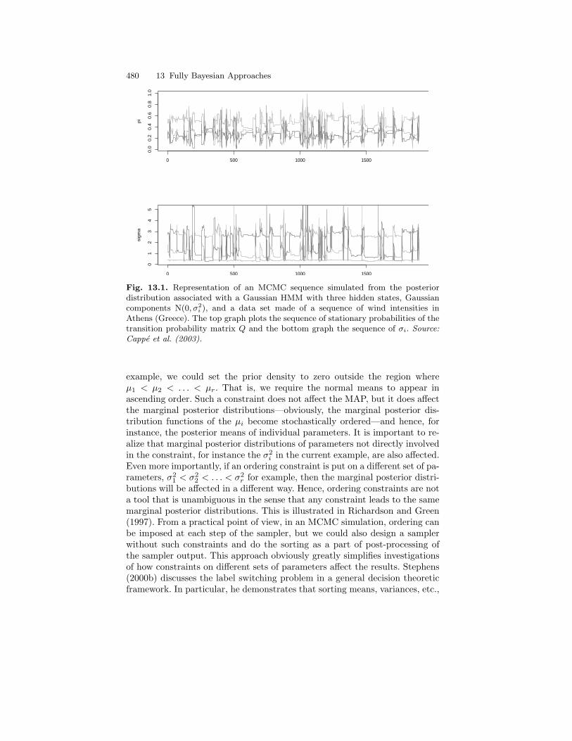
480 13 Fully Bayesian Approaches

0 500 1000 1500

0.0

0.2

0.4

0.6

0.8

1.0

pi

0 500 1000 1500

01

23

45

sigm

a

Fig. 13.1. Representation of an MCMC sequence simulated from the posteriordistribution associated with a Gaussian HMM with three hidden states, Gaussiancomponents N(0, σ2

i ), and a data set made of a sequence of wind intensities inAthens (Greece). The top graph plots the sequence of stationary probabilities of thetransition probability matrix Q and the bottom graph the sequence of σi. Source:Cappe et al. (2003).

example, we could set the prior density to zero outside the region whereµ1 < µ2 < . . . < µr. That is, we require the normal means to appear inascending order. Such a constraint does not affect the MAP, but it does affectthe marginal posterior distributions—obviously, the marginal posterior dis-tribution functions of the µi become stochastically ordered—and hence, forinstance, the posterior means of individual parameters. It is important to re-alize that marginal posterior distributions of parameters not directly involvedin the constraint, for instance the σ2

i in the current example, are also affected.Even more importantly, if an ordering constraint is put on a different set of pa-rameters, σ2

1 < σ22 < . . . < σ2

r for example, then the marginal posterior distri-butions will be affected in a different way. Hence, ordering constraints are nota tool that is unambiguous in the sense that any constraint leads to the samemarginal posterior distributions. This is illustrated in Richardson and Green(1997). From a practical point of view, in an MCMC simulation, ordering canbe imposed at each step of the sampler, but we could also design a samplerwithout such constraints and do the sorting as a part of post-processing ofthe sampler output. This approach obviously greatly simplifies investigationsof how constraints on different sets of parameters affect the results. Stephens(2000b) discusses the label switching problem in a general decision theoreticframework. In particular, he demonstrates that sorting means, variances, etc.,

13.1 Parameter Estimation 481

sometimes gives results that are difficult to interpret, and he suggests, in thecontexts of i.i.d. observations from a finite mixture, a relabeling algorithmbased on probabilities of the each observation belonging to a certain mixturecomponent.

If we put a sorting constraint on the parameters, we implicitly construct anew prior that is zero in regions where the constraint does not hold. Moreover,because a parameter can be permuted in r! different ways, the new prior isequal to the original prior multiplied by r! in the region where the constraintdoes hold, in order to make it integrate to unity (over the constrained space).A similar but slightly different view, suggested by Stephens (2000a), is tothink of the r! permutations of a given parameter as a single element of anequivalence class of parameters; the effective parameter space is then the spaceof such equivalence classes. Again, because a parameter of order r can bepermuted in r! different ways, each element of the equivalence class [θ] has aprior that is r! times the prior π(θ) of any of its particular representations θ.This distinction between a parameter and its corresponding equivalence classand the factor r! are not important when r is fixed, but it becomes importantwhen r is variable, and we attempt to estimate it, as discussed in Section 13.2.

Lack of identifiability can also be circumvented by using a loss functionthat is impervious to label switching, that is, invariant under permutation ofthe label indices. For instance, in the case of mixtures, Celeux et al. (2000)employed a loss function for the estimation of the parameter θ may based onthe Kullback-Leibler divergence,

loss(θ, θ) =∫

logp(y0:n|θ)p(y0:n|θ)

p(y0:n|θ) dy0:n .

13.1.4 MCMC Methods for Bayesian Inference

Analytic computation of Bayesian estimates like the posterior mean or poste-rior mode is most generally infeasible for HMMs, except for the simplest mod-els. We now review simulation-based methods that follow the general MCMCscheme introduced in Chapter 6 and provide Monte Carlo approximations ofthe posterior distribution of the parameters θ given the observable Y0:n. Asnoted in Chapter 6, the distribution of X0:n given both Y0:n and θ is oftenmanageable (when X is finite notably). Likewise, the conditional distributionof the parameters given Y0:n and X0:n is usually simple enough in HMMs, es-pecially when conjugate priors are used (as in Example 13.1.7). What remainsto be exposed here is how to bridge the gap between these two conditionals.

The realization that for HMMs, the distribution of interest involves twoseparate entities, θ and X0:n, for which the two conditional distributionsπ(θ|x0:n, y0:n) and π(x0:n|θ, y0:n) are available or may be sampled from, sug-gests the use of a two stage Gibbs sampling strategy as defined in Chapter 6(see Algorithm 6.2.13). The simplest version of the Gibbs sampler, which willbe referred to as global updating of the hidden chain, goes as follows.

482 13 Fully Bayesian Approaches

Algorithm 13.1.8. Iterate:

1. Simulate θ from π(θ|x1:n, y0:n).2. Simulate X0:n from π(x0:n|θ, y0:n).

This means that, if we can simulate the parameters based on the completedmodel (and this is usually the case, see Example 13.1.10 for instance) and themissing states X0:n conditionally on the parameters and Y0:n (see Chapter 6),we can implement this two-stage Gibbs sampler, also called data augmentationby Tanner and Wong (1987). We note that θ typically is multivariate, and itis then often broken down into several components; accordingly, the first stepabove then breaks down into several sub-steps. Similar comments apply ifthere are hyperparameters with their own priors in the model; we can viewthem as part of θ even though they are often updated separately.

By global updating we mean that the trajectory of the hidden chainis updated as a whole from its joint conditional distribution given the pa-rameter θ and the data Y0:n. This corresponds to the partitioning (θ,X0:n)of the state space of the Gibbs sampler. Another possible partitioning is(θ,X0, X1, . . . , Xn), which leads to an earlier and more “rudimentary” ver-sion of the Gibbs sampler (Robert et al., 1993). In this algorithm, only onehidden variable Xk is updated at a time, and we refer to this scheme as localupdating of the hidden chain. The algorithm thus looks as follows.

Algorithm 13.1.9. Iterate:

1. Simulate θ from π(θ|x1:n, y1:n).2. For k = 0, 1, . . . , n, simulate Xk from π(xk|θ, y1:n, x1:k−1, xk+1:n).

This algorithm only updates one state at a time, and, because

π(xk|θ, y0:n, x0:k−1, xk+1:n)

reduces to

π(xk|θ, yk, xk−1, xk+1) ∝ qθ(xk−1, xk)qθ(xk, xk+1)gθ(xk, yk)

where the first factor on the right-hand side is replaced by νθ(x0) for k = 0and the second factor is replaced by unity for k = n; this means that each Xk

is updated conditional upon its neighbors, as seen in Chapter 6.In the above algorithm, the Xk are updated in a fixed linear order, but

there is nothing that prevents us from using a different order or from pick-ing the variable Xk to be updated at random. Of course there are schemesintermediate between the extremes global and local updating. We might, forexample, update blocks of Xk; like for local updating, these blocks may beof fixed size and updated in a specific order, but size and order may also bechosen at random as in (Shephard and Pitt, 1997).

13.1 Parameter Estimation 483

Example 13.1.10 (Normal HMM, Continued). Let us return to theHMM and prior given in Example 13.1.7. To compute the respective full con-ditionals in the Gibbs sampler, we note again that each such distribution, ordensity, is proportional (in the component to be updated) to the product ofthe prior and the likelihood. For example,

π(µ1, . . . , µr|Q, σ21 , . . . , σ

2r , x1:n, y0:n)

∝ π(Q,µ1, . . . , µr, σ21 , . . . , σ

2r)

×p(x0:n|Q)L(y0:n|x0:n, µ1, . . . , µr, σ21 , . . . , σ

2r)

= π(Q)π(µ1) · · ·π(µr)π(σ21) · · ·π(σ2

r)p(x0:n|Q)n∏k=0

g(µ,σ)(xk, yk) .

By picking out the factors on the right-hand side that contain the appropriatevariables, we can find their full conditional. We now detail this process for eachof the variables involved.

The conditional pdf of µ1, . . . , µr is proportional to

r∏i=1

exp−(µi − α)2/2β

n∏k=0

exp−(yk − µxk)/2σ2

xk

∝

r∏i=1

exp−1

2[µ2i (β−1 + niσ

−2i )− 2µi(αβ−1 + Siσ

−2i )]

,

where ni is the number of xk with xk = i and Si is the sum of the corre-sponding yk; Si =

∑k: xk=i yk. We can conclude that the full conditional

distribution of µ1, . . . , µr is such that these variables are conditionally inde-pendent and

µi |Q, σ21 , . . . , σ

2r , x0:n, y0:n ∼ N

(ασ2

i /β + Siσ2i /β + ni

,1

1/β + ni/σ2i

). (13.7)

This can also be understood in the following way: given X0:n all the obser-vations are independent, and to obtain the posterior for µi we only need toconsider observations governed by this regime. As the µi are a priori inde-pendent, they will be so a posteriori as well. The above formula is then astandard result of Bayesian statistics (cf. Example 13.1.2).

In a similar fashion, one finds that

π(σ21 , . . . , σ

2r |Q,µ1, . . . , µr, x0:n, y0:n)

∝r∏i=1

(σ2i )−(κ+ni/2+1) exp

−(γ + S

(2)i /2)/σ2

i

,

where S(2)i =

∑k: xk=i(yk − µi)2. Hence, the full conditional distribution of

σ21 , . . . , σ

21 is such that these variables are conditionally independent, and

484 13 Fully Bayesian Approaches

σ2i |Q,µ1, . . . , µr, x0:n, y0:n ∼ IG(κ+ ni/2, (γ + S

(2)i /2)) . (13.8)

This result is indeed also an immediate consequence of Example 13.1.2.The full conditional distribution of the transition matrix Q was essentially

derived in Lemma 13.1.6; the rows are conditionally independent with the ithrow following a Dirichlet distribution Dirr(δ1 + nij , . . . , δr + nir). Here nij isthe number of transitions from state i to j, that is, nij = #0 ≤ k ≤ n− 1 :xk = i, xk+1 = j.

Several types of MCMC moves are typically put together in what is oftencalled a sweep of the algorithm. Thus, one sweep of the Gibbs sampler withlocal updating for the present model looks as follows.

Algorithm 13.1.11.

1. Simulate the µi independently according to (13.7).2. Simulate the σ2

i independently according to (13.8).3. Simulate the rows of Q independently, with the ith row from Dirr(δ1 +ni1, . . . , δr + nir).

4. For k = 0, 1, . . . , n, simulate Xk with unnormalized probabilities

P(Xk = i | θ, yk, xk−1, xk+1) ∝ q(xk−1, i)q(i, xk+1)1σi

e−(yk−µi)2/2σ2i ;

for k = 0 the first factor is replaced by ν(x0), and for k = n the factorq(i, xk+1) is replaced by unity.

If ν is the stationary distribution of Q, simulation of Q requires aMetropolis-Hastings step; a sensible proposal is then the same Dirichlet asabove. If ν is rather a separate parameter, Q is updated as above and, pro-vided the prior on (ν1, . . . , νr) is a Dirichlet as in Example 13.1.7, this vectoris updated with full conditional distribution Dirr(δ′1 + t1, . . . , δ

′r + tr) with

ti = 1x0 = i. Of course, global updating of X0:n could have been used aswell, which would modify step 4 of the algorithm only.

The Gibbs sampler with local updating should mix and explore the poste-rior surface much more slowly than when global updating is used. It must beconsidered, however, that the simulation of the whole vector of states, X1:n,is more time-consuming in that it requires the use of the forward or backwardformulas (Section 6.1.2). A numerical comparison of the two approaches byRobert et al. (1999), using several specially designed convergence monitoringtools, did not exhibit an overwhelming advantage in favor of global updating,even without taking into account the additional O(n2) computational time re-quired by this approach. On the other hand, Scott (2002) provided an exampleshowing a significant advantage for global updating in terms of autocovariancedecay. It is thus difficult to make a firm recommendation on which updatingscheme to use. One may start by running local updating, and if its mixingbehavior is poor, try global updating as well. We do remark, however, thatwhen the state space X is continuous, there is seldom any alternative to local

13.1 Parameter Estimation 485

updating. In addition, with continuous X, local updating must in general becarried out by a Metropolis-Hastings step, as the full conditional distributionseldom lends itself to direct simulation (see Section 6.3). The next exampledemonstrates a somewhat more complicated use of the single site Gibbs sam-pling strategy.

Example 13.1.12 (Capture-Recapture, Continued). Let us now con-sider Gibbs simulation from the posterior distribution of the parameters in thecapture-recapture model of Example 1.3.4. The parameters are divided into(a) the capture probabilities pk(i), indexed by the capture zone i (i = 1, 2, 3),and (b) the movement probabilities qk(i, j) (i, j = 1, 2, 3, †), which are theprobabilities that the lizard is in zone j at time k + 1 given that it is in zonei at time k. For instance, the probability qk(†, †) is equal to 1, because of theabsorbing nature of †. We also denote by ϕk(i) the survival probability at timek in zone i, that is,

ϕk(i) = 1− qk(i, †) ,

and by ψk(i, j) the effective probability of movement for the animals remainingin the system, that is,

ψk(i, j) = qk(i, j)/ϕk(i) .

If we denote ψk(i) = (ψk(i, 1), ψk(i, 2), ψk(i, 3)), the prior distributions arechosen to be

pk(i) ∼ Be(a, b), ϕk(i) ∼ Be(α, β), ψk(i) ∼ Dir3(γ1, γ2, γ3) ,

where the hyperparameters a, b, γ1, γ2, γ3 are known.The probabilities of capture pk(i) depend on the zone of capture i and

the missing data structure of the model, which must be taken into account.Slightly modifying the notations of Example 1.3.4, we let y∗km be the positionof animal m at time k and xkm its capture indicator, the observations canbe written in the form ykm = xkmy

∗km, where ykm = 0 corresponds to a

missing observation. The sequence of y∗km for a given m then correspondsto a non-homogeneous Markov chain, with transition matrix Qk = (qk(i, j)).Conditionally on y∗km, the Xkm then are Bernoulli variables with probabilityof success pk(y∗km).

The Gibbs sampler associated with this model has the following steps.

Algorithm 13.1.13.

1. Simulate y∗km for sites such that xkm = 0.2. Generate (0 ≤ k ≤ n)

pk(i) ∼ Be(a+ uk(i), b+ vk(i)) ,ϕk(m) ∼ Be(α+ wk(i), β + wk(i, †)) ,ψk(i) ∼ Dir3(γ1 + wk(i, 1), γ2 + wk(i, 2), γ3 + wk(i, 3)) ,

486 13 Fully Bayesian Approaches

where uk(i) denotes the number of captures in i at time k, vk(i) the numberof animals unobserved at time i for which the simulated ykm is equal to i,wk(i, j) the number of passages (observed or simulated) from i to j, wk(i, †)the number of (simulated) passages from i to †, and

wk(i) = wk(i, 1) + wk(i, 2) + wk(i, 3) .

Step 1. must be decomposed into conditional sub-steps to account for theMarkovian nature of the observations; in a full Gibbs strategy, y∗km can besimulated conditionally on y∗(k−1)m and y∗(k+1)k when xkm = 0. If k 6= n, themissing data are simulated according to

P(y∗km = j | y∗(k−1)m = i, y∗(k+1)m = `, xkm = 0) ∝ qk−1(i, j)(1− pk(j))qk(j, `)

andP(y∗nm = j | y∗(n−1)m = i, xnm = 0) ∝ qn−1(i, j)(1− pn(j)) .

So far, we have dealt with MCMC algorithms for which the state space ofthe sampler consists of the parameter θ and the hidden chain X0:n; both arerandom, unobserved quantities—θ because we are in a Bayesian frameworkand X0:n because of its role in the model as a latent variable. However, it isquite possible to devise MCMC algorithms for which the sampler state spacecomprises θ alone and not the hidden chain. In particular, when the state spaceX of the hidden chain is finite, we know that the likelihood may be computedexactly. In such a case the completion step, that is, the simulation of X0:n,does not appear as a necessity any longer, and alternative Metropolis-Hastingssteps can be used instead.

Example 13.1.14 (Normal HMM, Continued). In Cappe et al. (2003),the simulation of the parameters of the normal components, as well as ofthe parameters of the transition probability matrix, was done through simplerandom walk proposals: for the means µj the proposed move is

µ′j = µj + εi ,

where εi ∼ N(0, τµ) and τµ is a parameter that may be adjusted to optimizeperformance of the sampler. Because the proposal is symmetric, the accep-tance ratio is simple; it is

π(θ′)L(y0:n|θ′)π(θ)L(y0:n|θ)

,

where L is the likelihood computed via the forward algorithm (Section 5.1.1).For the variances σ2

j , the proposed move is a multiplicative random walk

log σ′j = log σj + εj ,

where εj ∼ N(0, τσ), with acceptance ratio

13.1 Parameter Estimation 487

π(θ′)L(y0:n|θ′)π(θ)L(y0:n|θ)

∏j

σ′jσj

,

the last term being the ratio of the Jacobians incurred by working on the log-scale. To describe the above proposal, we also sometimes say that σ′j followsa log-normal LN(log σj , τσ) distribution.

In the case of the transition probability matrix, Q, the move is slightlymore involved due to the constraint on the sums of the rows, Q being astochastic matrix. Cappe et al. (2003) solved this difficulty by reparameteriz-ing each row (qi1, . . . , qir) as

qij =ωij∑` ωi`

, ωij > 0 ,

so that the summation constraint on the qij does not hinder the random walk.Obviously the ωij are not identifiable, but as we are only interested in the qij ,this is not a true difficulty. On the opposite, using overparameterized represen-tations often helps with the mixing of the corresponding MCMC algorithms,as they are less constrained by the data set or the likelihood. The proposedmove on the ωij is

logω′ij = logωij + εij ,

where εij ∼ N(0, τω), with acceptance ratio

π(θ′)L(y0:n|θ′)π(θ)L(y0:n|θ)

∏i,j

ω′ijωij

.

Note that this reparameterization of the model forces us to select a priordistribution on the ωij rather than on the qij . The choice ωij ∼ Ga(δj , 1) isnatural in that it gives a Dirr(δ1, . . . , δr) distribution on the corresponding(qi1, . . . , qir). We also note that it is not difficult to show that if (ωi1, . . . , ωir) isreparameterized into Si =

∑r1 ωij and (qi1, . . . , qir), then, given x0:n, Si and

(qi1, . . . , qir) are conditionally independent and distributed as Ga(∑r

1 δj , 1)and Dirr(δ1+ni1, . . . , δr+nir) respectively. This proves that the ω-parameter-ization does nothing but introduce a new parameter for each row, the sumSi, that is independent of everything else and hence totally irrelevant for theinference. The point of introducing this extra variable is only to simplify thedesign of Metropolis-Hastings moves. If the initial distribution ν is also aparameter of the model, it can be recast in a similar fashion.

Figure 13.1 provides an illustration of this simulation scheme in the specialcase of a Gaussian HMM with zero means. Over the 2,000 MCMC iterationsrepresented on both graphs, there are periods where the value of the σi orof the stationary probabilities of Q do not change: these periods correspondto sequences of proposed values that are rejected at the Metropolis-Hastingsstage. Note that the rejection periods are not the same for the σi and thestationary probabilities. This is due to the fact that there is a Metropolis-Hastings stage for each group of parameters.

488 13 Fully Bayesian Approaches

Another alternative stands at the opposite end of the range of possibilities:the parameters of the model can be integrated out when conjugate priors areused, as demonstrated by Liu (1994), Chen and Liu (1996), and Casella et al.(2000) in the case of mixture and switching regression models. In such schemes,each site Xk is typically sampled conditionally on all the other sites, with themodel parameters fully integrated out.

13.2 Reversible Jump Methods

So far we have not touched upon the topic of the unknown number of statesin an HMM and of the estimation of this number via Bayesian procedures.After a short presentation of variable dimension models and of their meaning,we introduce the adequate MCMC methodology to deal with this additionallevel of complexity.

13.2.1 Variable Dimension Models

In general, a variable dimension model is, to quote Peter Green, a “modelwhere one of the things you do not know is the number of things you do notknow”. In other words, this pertains to a statistical model where the dimensionof the parameter space is not “known”. This is not a formal enough definition,obviously, and we need to provide a more rigorous perspective.

Definition 13.2.1 (Variable Dimension Model). A variable dimensionmodel is defined as a collection of models (or parameter spaces),

Θr, r = 1, . . . , R ,

associated with a collection of priors on these spaces,

πr(θr), r = 1, . . . , R ,

and a prior distribution on (the indices of) these spaces,

%(r), r = 1, . . . , R .

In the following, we shall consider that a variable dimension model isassociated with a probability distribution on the space

Θ =R⋃r=1

r ×Θr , (13.9)

where the union is of course one of disjoint sets. An element θ of Θ may thusalways be written as θ = (r, θr), where θr is an element of Θr. Obviously, thisconvention is somewhat redundant, as we generally know by looking at the

13.2 Reversible Jump Methods 489

second component of θ to which of the sets in (13.9) θ belongs, but it willgreatly simplify matters from a notational point of view. The target densitywill be denoted by

π(θ) = π(r, θr) = %(r)πr(θr) .

In order to avoid tedious (but straightforward) constructions, we do not fullyspecify the dominating measure used for defining the above density, and wewill also, when needed and unambiguous from the context, use the notationπ(dθ) to refer to the probability measure itself. On the individual parameterspaces Θr, we denote the dominating measure by dθr as previously.

For HMMs, the space Θr is in general that of parameters for HMMs withr states for the hidden Markov chain. We remark that strictly speaking, amodel is not identical to a parameter space, as the parameter space alonedoes not tell anything about the model structure. Two completely differentmodels could well have identical parameter spaces. In the development below,this distinction between model and parameter space is not important however,and we will work with the parameter spaces only.

In the Bayesian framework exposed above, the dimension r of the modelis treated as a usual parameter. The aim is to address the two problemsof testing—deciding which model is best—and estimation—determining theparameters of the best fitting model—simultaneously. Conceptually, a variabledimension model is more complicated only because the prior and posteriordistributions live in the space Θ defined in (13.9), whose structure is quitecomplex. Interestingly, by integrating out the index part of the model, wesimply end up with mixture representations both for the distribution of thedata,

R∑r=1

%(r)p(y) ,

and for the predictive distribution (given observations yobs)

R∑r=1

%(r|yobs)∫p(y|θr)πr(θr|yobs) dθr .

This mixture representation, called model averaging in the Bayesian literature,is interesting because it suggests the use of predictors that are not obtainedby selecting a particular model from the R possible ones but rather consist intaking all the options into account simultaneously, weighting them by theirposterior odds %(r|yobs). The variability due to the selection of the model isthus accounted for.

Note also that in defining the variable dimension model, we have chosena completely new set of parameters for each model Θr and set the parameterspace as the union of the model parameter spaces Θr, even though someparameters may have a similar meaning in two different models. For instance,when comparing an AR(p) and an AR(p+ 1) model, it could be posited that

490 13 Fully Bayesian Approaches

the first p autoregressive coefficients would remain the same for the AR(p) andAR(p + 1) models, i.e., that an AR(p) model is simply an AR(p + 1) modelwith an extra zero coefficient. We argue on the opposite that they should bedistinguished as entities because the models are different and also because,for instance, the best fitting AR(p + 1) model is not necessarily a straightmodification of the best fitting AR(p) model by adding an extra term whilekeeping the other ones fixed. Similarly, even though the variance σ2 has thesame formal meaning for all values of p in the autoregressive case, we insiston using a different variance parameter for each value of p.

This is not the only possible perspective on this problem however, andmany prefer to use some parameters common to all models in order to re-duce model and computational complexity. In some sense, the reversible jumptechnique to be discussed in Section 13.2.3 is based on this assumption ofexchangeable parameters between models, using proposal distributions thatmodify only a part of the parameter vector to move between models.

Given a variable dimension model, there is an additional computationaldifficulty in representing, or simulating from, the posterior distribution in thata sampler must move both within and between models Θr. Although the formerpertains to previous developments (Section 13.1.4), the latter requires a soundmeasure-theoretic basis to lead to correct MCMC moves, that is, to movesthat validate π(θ|y0:n) as the stationary distribution of the simulated Markovchain. There have been several earlier approaches in the literature, using forinstance birth-and-death processes (Geyer and Møller, 1994) or pseudo-priors(Carlin and Chib, 1995), but the general formalization of this problem hasbeen realized by Green (1995).

13.2.2 Green’s Reversible Jump Algorithm

Green’s (1995) algorithm is basically of Metropolis-Hastings type with spe-cific trans-dimensional proposals carefully designed to move between differentmodels in a way that is consistent with the desired stationary distribution ofthe MCMC algorithm. We discuss here only the simplest, and more common,application of Green’s ideas in which the moves from higher to lower dimen-sional models are deterministic and refer to Green (1995) or Richardson andGreen (1997) for more involved proposals.

We describe below the structure of moves between two different modelsΘs and Θl, where Θl say is of larger dimension than is Θs (“s” is for smalland “l” for large). If the Markov chain is currently in state θs ∈ Θs, Green’salgorithm uses an auxiliary random variable, which we denote by v, and afunction m that maps the pair (θs, v) into a proposed new state θl ∈ Θl. Theonly requirement is that m be differentiable with an inverse mapping m−1

that is also differentiable. If (θs, v) is the point that corresponds to θl troughm−1, we will use the notations

θs = m−1param(θl) and v = m−1

aux(θl)

13.2 Reversible Jump Methods 491

for the associated projections of m−1(θl). The reverse move from Θl to Θsis deterministic and simply consists in jumping back to the point θs =m−1

param(θl). Obviously, this dimension-changing move alone may fail to ex-plore the whole space, and it is necessary to propose usual fixed dimensionmoves as well as these trans-dimensional moves. For the moment we can ig-nore this fact however, as we are going to show that the trans-dimensionalmove alone is π reversible. We shall assume that when in state θs ∈ Θs, themove to Θl is attempted with probability Ps,l and that the auxiliary variablev has a density p. Conversely, when in Θl, the move to Θs is attempted withprobability Pl,s. The moves are then accepted with probability α(θs, θl) in thefirst case and α(θl, θs) in the second one, where it is understood that the chainstays in its current state in case of rejection.

To determine the correct form of the acceptance probability α, we willcheck that the transition kernel corresponding to the mechanism describedabove does satisfy the detailed balance condition (2.12) for the target π. Afirst remark is that given the structure of the state space Θ, which is a unionof disjoint sets, one can fully specify probability distributions on Θ by theiroperation on test functions fq of the form

fq(θ) = fq(r, θr) =

0 if r 6= q ,fr(θr) otherwise , (13.10)

for some q = 1, . . . , R and fq ∈ Fb (Θq). For such a test function,

Eπ(fq) = %(q)∫Θq

fq(θq)πq(θq) dθq .

The second important remark is that when examining the proof of the re-versibility of the usual Metropolis-Hastings algorithm (Proposition 6.2.6), itis seen that the form of the acceptance probability α is entirely determined bywhat happens when the chain really moves. The part that concerns rejectionis fully determined by the fact that the transition kernel must be a probabilitykernel, that is, integrate to unity. Hence, in the case under consideration, wemay check the detailed balance condition for test functions of the form givenin (13.10) only, with q = s and q = l. We will denote these functions by fsand fl respectively (with associated functions fs ∈ Fb (Θs) and fl ∈ Fb (Θl)).

Denoting by K the transition kernel associated with the move between Θsand Θl described above, we have∫∫

fs(θ)π(dθ)×K(θ, dθ′)fl(θ′) =∫%(s)πs(θs)fs(θs)

∫Ps,l α[θs,m(θs, v)]p(v)fl[m(θs, v)] dv

dθs .

Now apply the change of variables formula to replace the pair (θs, v) by θl.This yields

492 13 Fully Bayesian Approaches∫∫fs(θ)π(dθ)×K(θ, dθ′)fl(θ′) =∫fs[m−1

param(θl)]fl(θl)%(s)πs(m−1param(θl))

Ps,lα(θs, θl)p[m−1aux(θl)]

Js,l(θl)dθl ,

(13.11)

where Js,l(θl) is the absolute value of the determinant of the Jacobian matrixassociated with the mapping m. It may be evaluated either as

Js,l(θl) =∣∣∣∣∂m(θs, v)∂(θs, v)

∣∣∣∣(θs,v)=m−1(θl)

or

Js,l(θl) =∣∣∣∣∂m−1(θl)

∂θl

∣∣∣∣−1

.

Because the reverse move is deterministic, the opposite case is much simplerand∫∫

fl(θ)π(dθ)×K(θ, dθ′)fs(θ′) =∫%(l)πl(θl)fl(θl)

Pl,sα[θl,m−1

param(θl)]fs[m−1param(θl)]

dθl . (13.12)

To ensure that (13.11) and (13.12) coincide for all choices of the functions fsand fl, the acceptance probability must satisfy

%(s)πs(θs)Ps,lp(v)Js,l(θl)

α(θs, θl) = %(l)πl(θl)Pl,sα(θl, θs) , (13.13)

where it is understood that θs, θl and v satisfy θl = m(θs, v). By analogy withthe case of the usual Metropolis-Hastings algorithm, it is possible to find asolution to the above equation of the form

α(θs, θl) = A(θs, θl) ∧ 1 and α(θl, θs) = A−1(θs, θl) ∧ 1

by setting

A(θs, θl) =%(l)πl(θl)Pl,s

%(s)πs(θs)Ps,lp(v)Js,l(θl) . (13.14)

Indeed, with this choice both sides of (13.13) evaluate to

%(l)πl(θl)Pl,s ∧%(s)πs(θs)Ps,lp(v)

Js,l(θl).

Thus (13.14) defines the applicable acceptance ratio to be used withGreen’s reversible jump move. At this level the formulation of Green’s al-gorithm is rather abstract, but we hope it will be more clear after studyingthe following example.

13.2 Reversible Jump Methods 493

Example 13.2.2 (Normal HMM, Continued). We shall extend Exam-ple 13.1.14 to allow for moving between HMMs of different orders usingreversible jump MCMC. We will discuss two different kinds of dimension-changing moves, or, rather, pair of moves: birth/death and split/combine. Ina birth move, the order of the Markov chain is increased by one by adding anew state, and the death move works in the reverse way by deleting an exist-ing state. The split move takes an existing state and splits it in two, whereasthe combine (also called merge) move takes a pair of states and tries to com-bine them into one. We will now in detail describe these moves and how theiracceptance ratios are computed.

We start with the birth move. Suppose that the current MCMC state is(r, θr), and that we attempt to add a new state, that we denote by i0, to theHMM. We first draw the random variables

µi0 ∼ N(α, β), σ2i0∼ IG(κ, γ),

ωi0,j ∼ Ga(δj , 1) for j = 1, . . . , r, ωi,i0 ∼ Ga(δi0 , 1) for i = 1, . . . , r,

ωi0,i0 ∼ Ga(δi0 , 1),

all independently. In other words, the parameters that go with the new stateare drawn from their respective priors. These parameters correspond to theauxiliary variable vbirth for the birth move. The remaining parameters, thatis, the components of θr, are simply copied to the proposed new state θr+1.Therefore, the corresponding mapping mbirth is simply the identity; no par-ticular transformation is required to obtain the proposed new state in Θr+1.In the death move, the attempted move is to delete a state, denoted by i0,that is chosen at random. The auxiliary variables µi0 , etc., of the associatedbirth move are trivially recovered; they are just components of the state i0that is proposed to be deleted!

Next in turn is the computation of the acceptance ratio, which is in factquite simple in this particular case. Because the mapping mbirth is the iden-tity mapping, its Jacobian is the identity matrix, with determinant one. Theremaining factors of (13.14) become

%(r + 1)πr+1(θr+1)L(y0:n|θr+1)(r + 1)!%(r)πr(θr)L(y0:n|θr)r!

× Pd(r + 1)/(r + 1)Pb(r)

× 1pµ(µi0)pσ2(σ2

i0)∏ri=1 pω(ωi,i0)

∏rj=1 pω(ωi0,j)pω(ωi0,i0)

. (13.15)

This ratio deserves some further comments. The first factor is the ratio ofposterior densities. The factorials arise from the fact that, as the prior isexchangeable—the prior as well as the posterior are invariant under permu-tations of states—we cannot distinguish between parameters that are identi-cal up to such permutations. Thus our effective parameter space for r-orderHMMs is that of equivalence classes of parameters that are identical up to

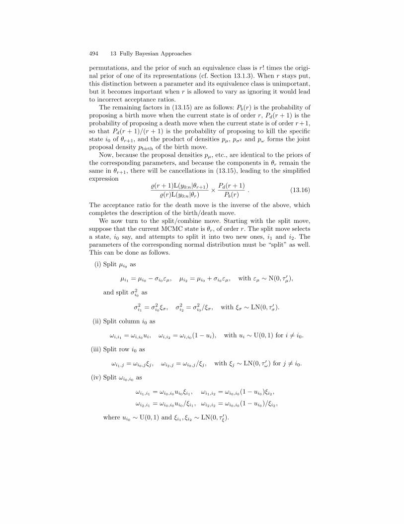
494 13 Fully Bayesian Approaches

permutations, and the prior of such an equivalence class is r! times the origi-nal prior of one of its representations (cf. Section 13.1.3). When r stays put,this distinction between a parameter and its equivalence class is unimportant,but it becomes important when r is allowed to vary as ignoring it would leadto incorrect acceptance ratios.

The remaining factors in (13.15) are as follows: Pb(r) is the probability ofproposing a birth move when the current state is of order r, Pd(r + 1) is theprobability of proposing a death move when the current state is of order r+1,so that Pd(r + 1)/(r + 1) is the probability of proposing to kill the specificstate i0 of θr+1, and the product of densities pµ, pσ2 and pω forms the jointproposal density pbirth of the birth move.

Now, because the proposal densities pµ, etc., are identical to the priors ofthe corresponding parameters, and because the components in θr remain thesame in θr+1, there will be cancellations in (13.15), leading to the simplifiedexpression

%(r + 1)L(y0:n|θr+1)%(r)L(y0:n|θr)

× Pd(r + 1)Pb(r)

. (13.16)

The acceptance ratio for the death move is the inverse of the above, whichcompletes the description of the birth/death move.

We now turn to the split/combine move. Starting with the split move,suppose that the current MCMC state is θr, of order r. The split move selectsa state, i0 say, and attempts to split it into two new ones, i1 and i2. Theparameters of the corresponding normal distribution must be “split” as well.This can be done as follows.

(i) Split µi0 as

µi1 = µi0 − σi0εµ, µi2 = µi0 + σi0εµ, with εµ ∼ N(0, τ ′µ),

and split σ2i0

as

σ2i1 = σ2

i0ξσ, σ2i2 = σ2

i0/ξσ, with ξσ ∼ LN(0, τ ′σ).

(ii) Split column i0 as

ωi,i1 = ωi,i0ui, ωi,i2 = ωi,i0(1− ui), with ui ∼ U(0, 1) for i 6= i0.

(iii) Split row i0 as

ωi1,j = ωi0,jξj , ωi2,j = ωi0,j/ξj , with ξj ∼ LN(0, τ ′ω) for j 6= i0.

(iv) Split ωi0,i0 as

ωi1,i1 = ωi0,i0ui0ξi1 , ωi1,i2 = ωi0,i0(1− ui0)ξi2 ,

ωi2,i1 = ωi0,i0ui0/ξi1 , ωi2,i2 = ωi0,i0(1− ui0)/ξi2 ,

where ui0 ∼ U(0, 1) and ξi1 , ξi2 ∼ LN(0, τ ′ξ).

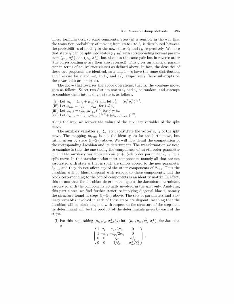
13.2 Reversible Jump Methods 495

These formulas deserve some comments. Step (ii) is sensible in the way thatthe transition probability of moving from state i to i0 is distributed betweenthe probabilities of moving to the new states i1 and i2, respectively. We notethat state i0 can be split into states (i1, i2) with corresponding normal param-eters (µi1 , σ

2i1

) and (µi2 , σ2i2

), but also into the same pair but in reverse order(the corresponding ω are then also reversed). This gives an identical param-eter in terms of equivalence classes as defined above. In fact, the densities ofthese two proposals are identical, as u and 1− u have the same distribution,and likewise for ε and −ε, and ξ and 1/ξ, respectively (here subscripts onthese variables are omitted).

The move that reverses the above operations, that is, the combine move,goes as follows. Select two distinct states i1 and i2 at random, and attemptto combine them into a single state i0 as follows.

(i’) Let µi0 = (µi1 + µi2)/2 and let σ2i0

= (σ2i1σ2i2

)1/2.(ii’) Let ωi,i0 = ωi,i1 + ωi,i2 for i 6= i0.(iii’) Let ωi0,j = (ωi1,jωi2,j)

1/2 for j 6= i0.(iv’) Let ωi0,i0 = (ωi1,i1ωi2,i1)1/2 + (ωi1,i2ωi2,i2)1/2.

Along the way, we recover the values of the auxiliary variables of the splitmove.

The auxiliary variables εµ, ξσ, etc., constitute the vector vsplit of the splitmove. The mapping msplit is not the identity, as for the birth move, butrather given by steps (i)–(iv) above. We will now detail the computation ofthe corresponding Jacobian and its determinant. The transformation we needto examine is thus the one taking the components of an rth order parameterθr and the auxiliary variables into an (r + 1)-th order parameter θr+1 by asplit move. In this transformation most components, namely all that are notassociated with state i0 that is split, are simply copied to the new parameterθr+1, and they do not affect any of the other components of θr+1. Thus theJacobian will be block diagonal with respect to these components, and theblock corresponding to the copied components is an identity matrix. In effect,this means that the Jacobian determinant equals the Jacobian determinantassociated with the components actually involved in the split only. Analyzingthis part closer, we find further structure implying diagonal blocks, namelythe structure found in steps (i)–(iv) above. The sets of parameters and aux-iliary variables involved in each of these steps are disjoint, meaning that theJacobian will be block diagonal with respect to the structure of the steps andits determinant will be the product of the determinants given by each of thesteps.

(i) For this step, taking (µi0 , εµ, σ2i0, ξσ) into (µi1 , µi2 , σ

2i1, σ2i1

), the Jacobianis

1 σi0 εµ/2σi0 01 −σi0 −εµ/2σi0 00 0 ξσ σ2

i00 0 1/ξσ −σ2

i0/ξ2σ

,

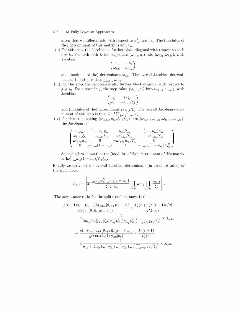
496 13 Fully Bayesian Approaches

given that we differentiate with respect to σ2i0

, not σi0 . The (modulus ofthe) determinant of this matrix is 4σ3

i0/ξσ.

(ii) For this step, the Jacobian is further block diagonal with respect to eachi 6= i0. For each such i, the step takes (ωi,i0 , ui) into (ωi,i1 , ωi,i2), withJacobian (

ui 1− uiωi,i0 −ωi,i0

)and (modulus of the) determinant ωi,i0 . The overall Jacobian determi-nant of this step is thus

∏i6=i0 ωi,i0 .

(iii) For this step, the Jacobian is also further block diagonal with respect toj 6= i0. For a specific j, the step takes (ωi0,j , ξj) into (ωi1,j , ωi2,j), withJacobian (

ξj 1/ξjωi0,j −ωi0,j/ξ2

j

)and (modulus of the) determinant 2ωi0,j/ξj . The overall Jacobian deter-minant of this step is thus 2r−1

∏j 6=i0 ωi0,j/ξj .

(iv) For this step, taking (ωi0,i0 , ui0 , ξi1 , ξi2) into (ωi1,i1 , ωi1,i2 , ωi2,i1 , ωi2,i2),the Jacobian is

ui0ξi1 (1− ui0)ξi2 ui0/ξi1 (1− ui0)/ξi1ωi0,i0ξi1 −ωi0,i0ξi2 ωi0,i0/ξi1 −ωi0,i0/ξi2ωi0,i0ui0 0 −ωi0,i0ui0/ξ2

i10

0 ωi0,i0(1− ui0) 0 −ωi0,i0(1− ui0)/ξ2i2

.

Some algebra shows that the (modulus of the) determinant of this matrixis 4ω3

i0,i0ui0(1− ui0)/ξi1ξi2 .

Finally we arrive at the overall Jacobian determinant (in absolute value) ofthe split move,

Jsplit =

∣∣∣∣∣∣2r+3σ3i0ω3i0,i0

ui0(1− ui0)ξσξi1ξi2

∏i 6=i0

ωi,i0∏j 6=i0

ωi0,jξj

∣∣∣∣∣∣ .The acceptance ratio for the split/combine move is thus

%(r + 1)πr+1(θr+1)L(y0:n|θr+1)(r + 1)!%(r)πr(θr)L(y0:n|θr)r!

× Pc(r + 1)/[(r + 1)r/2]Ps(r)/r

× 12pεµ(εµ)pξσ (ξσ)pξi1 (ξi1)pξi2 (ξi2)

∏j 6=i0 pξj (ξj)

× Jsplit

=%(r + 1)πr+1(θr+1)L(y0:n|θr+1)

%(r)πr(θr)L(y0:n|θr)× Pc(r + 1)

Ps(r)

× 1pεµ(εµ)pξσ (ξσ)pξi1 (ξi1)pξi2 (ξi2)

∏j 6=i0 pξj (ξj)

× Jsplit .

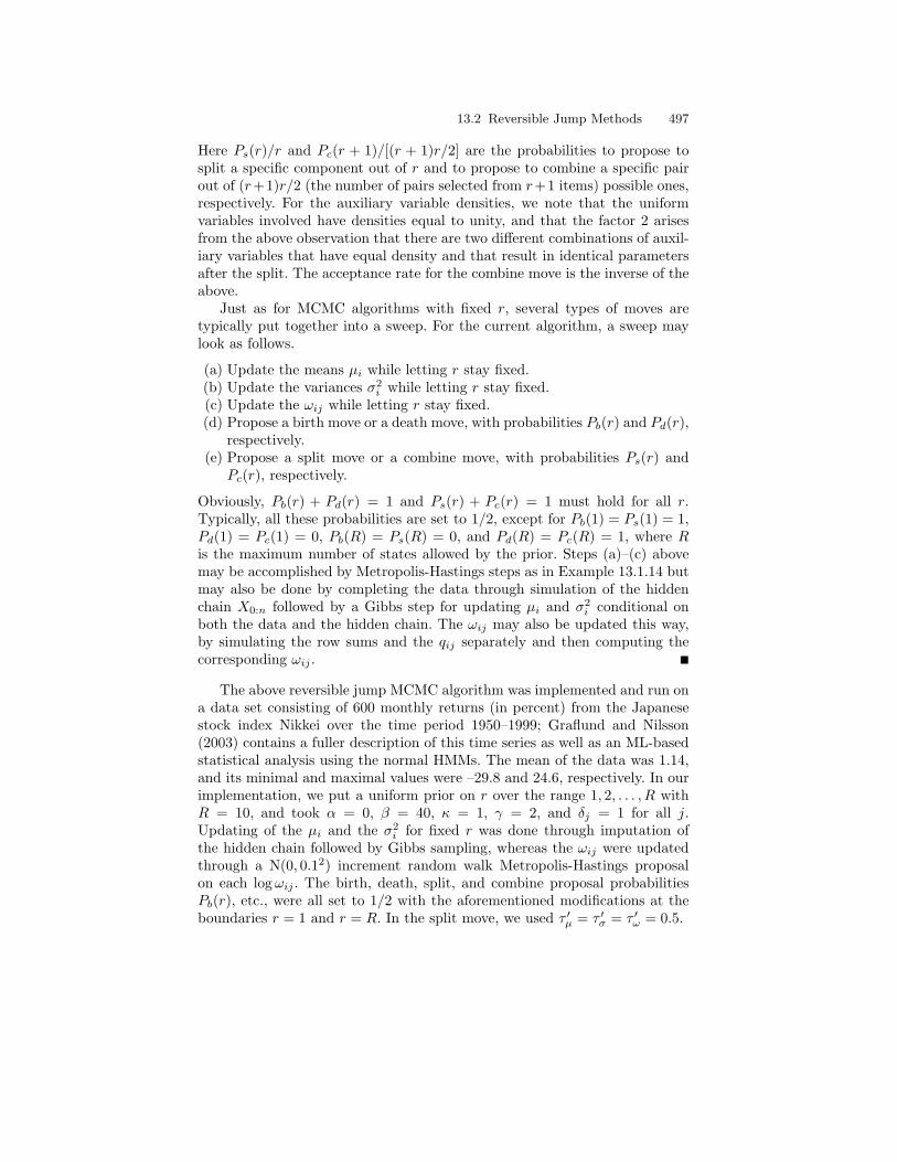
13.2 Reversible Jump Methods 497

Here Ps(r)/r and Pc(r + 1)/[(r + 1)r/2] are the probabilities to propose tosplit a specific component out of r and to propose to combine a specific pairout of (r+1)r/2 (the number of pairs selected from r+1 items) possible ones,respectively. For the auxiliary variable densities, we note that the uniformvariables involved have densities equal to unity, and that the factor 2 arisesfrom the above observation that there are two different combinations of auxil-iary variables that have equal density and that result in identical parametersafter the split. The acceptance rate for the combine move is the inverse of theabove.

Just as for MCMC algorithms with fixed r, several types of moves aretypically put together into a sweep. For the current algorithm, a sweep maylook as follows.

(a) Update the means µi while letting r stay fixed.(b) Update the variances σ2

i while letting r stay fixed.(c) Update the ωij while letting r stay fixed.(d) Propose a birth move or a death move, with probabilities Pb(r) and Pd(r),

respectively.(e) Propose a split move or a combine move, with probabilities Ps(r) and

Pc(r), respectively.

Obviously, Pb(r) + Pd(r) = 1 and Ps(r) + Pc(r) = 1 must hold for all r.Typically, all these probabilities are set to 1/2, except for Pb(1) = Ps(1) = 1,Pd(1) = Pc(1) = 0, Pb(R) = Ps(R) = 0, and Pd(R) = Pc(R) = 1, where Ris the maximum number of states allowed by the prior. Steps (a)–(c) abovemay be accomplished by Metropolis-Hastings steps as in Example 13.1.14 butmay also be done by completing the data through simulation of the hiddenchain X0:n followed by a Gibbs step for updating µi and σ2

i conditional onboth the data and the hidden chain. The ωij may also be updated this way,by simulating the row sums and the qij separately and then computing thecorresponding ωij .

The above reversible jump MCMC algorithm was implemented and run ona data set consisting of 600 monthly returns (in percent) from the Japanesestock index Nikkei over the time period 1950–1999; Graflund and Nilsson(2003) contains a fuller description of this time series as well as an ML-basedstatistical analysis using the normal HMMs. The mean of the data was 1.14,and its minimal and maximal values were –29.8 and 24.6, respectively. In ourimplementation, we put a uniform prior on r over the range 1, 2, . . . , R withR = 10, and took α = 0, β = 40, κ = 1, γ = 2, and δj = 1 for all j.Updating of the µi and the σ2

i for fixed r was done through imputation ofthe hidden chain followed by Gibbs sampling, whereas the ωij were updatedthrough a N(0, 0.12) increment random walk Metropolis-Hastings proposalon each logωij . The birth, death, split, and combine proposal probabilitiesPb(r), etc., were all set to 1/2 with the aforementioned modifications at theboundaries r = 1 and r = R. In the split move, we used τ ′µ = τ ′σ = τ ′ω = 0.5.

498 13 Fully Bayesian Approaches

The algorithm was run for 100,000 burn-in sweeps and then for another2,000,000 sweeps during which its output was monitored. The acceptance ratefor the update-ωij move, the split/combine move, and the birth/death movewas about 34%, 1.8%, and 1.4%, respectively. A higher rate for the dimension-changing moves would indeed be desirable, and this could perhaps be achievedwith modified moves. We did some experimentation with other values for κ,γ, and the τ ′, but without obtaining much variation in the acceptance rates.

The estimated posterior probabilities for r were 0.000, 0.307, 0.500, 0.156,0.029, 0.006, and 0.001 for r = 1, 2, . . . , 7 and below 0.001 for larger r. Graflundand Nilsson (2003) estimated the same kind of HMM from the data but usingML implemented through simulated annealing, arriving at the estimated p-value 0.60 for testing r = 2 vs. r = 3. They thus adopted r = 2 as their orderestimate, whereas the reversible jump MCMC analysis above gives the largestposterior probability for r = 3. However, our particular choice of prior mayhave a substantial effect on the posterior for r, and a Bayes factor analysis,which we did not carry out, may also give a different conclusion. Indeed,hierarchical priors are often used to attenuate the effect of the prior on theposterior (Richardson and Green, 1997; Robert et al., 2000). We stress that thealgorithm outlined above should be viewed as an example of a reversible jumpMCMC algorithm that may be modified and tuned for different applications,rather than as a “ready-to-use” algorithm that suits every need. As anotherexample of posterior analysis, we extracted the MCMC samples with r = 2components, permuted the component indices for each such sample to makethe means µi sorted (there was label switching in the MCMC output), andcomputed the posterior means: µ1 = 0.755 and µ2 = 1.568. This is to becompared to the MLEs µ1 = 0.847 and µ2 = 1.531 reported by Graflund andNilsson (2003). The credibility intervals we obtained were quite wide; the 95%intervals for µ1 and µ2 (after sorting) read (−0.213, 1.460) and (1.102, 2.074)respectively, both covering the respective MLE.

13.2.3 Alternative Sampler Designs

Reversible jump MCMC algorithms have in common with more conventionalMetropolis-Hastings algorithms that they generally contain some parametersthat need to be “fine tuned” in order to optimize their performance. In theexample above, these parameters are τ ′µ, τ ′σ and τ ′ω. Often the only way todo this fine tuning is through a set of pilot runs during which acceptanceprobabilities and other statistics related to the mixing of the algorithm aremonitored.

For any particular variable-dimension statistical model, there is an infinitenumber of ways of designing reversible jump algorithms. The above example isonly one of them for the normal HMM. Other structures of the split/combinemove, for instance, may prove more efficient with certain combinations ofpriors and/or data. Designing a reversible jump algorithm is by no means anautomated procedure but needs to be guided by experimentation and, when

13.2 Reversible Jump Methods 499

available, experience. The recent paper by Brooks et al. (2003) does outline,however, some general ideas about how to construct efficient reversible jumpalgorithms by setting up rules to calibrate the jump proposals.

Above, we motivated the factorial r! that is adjoined to the posterior den-sity by an argument based on equivalence classes of parameters. Richardsonand Green (1997) motivated them by saying that the actual parameter spaceis the one only containing parameters such that the normal means, for in-stance, appear in ascending order: µ1 < µ2 < . . . < µr, cf. Section 13.1.3. Wenote that sorting of this kind may become necessary even without restrictionson the prior, as we have seen that with an exchangeable prior, the marginalposterior densities of the means, for example, are generally identical. We pre-fer to view such sorting as a part of the post-processing of the MCMC sampleroutput, however, rather than as an intrinsic property of the algorithm itself.Sorting afterwards simplifies, for example, examination of how sorting withrespect to different sets of parameters (means or variances, for example) affectthe inference.

As a consequence of the assumption of sorted means, Richardson andGreen (1997) also restrict the split move, disallowing it to separate the nor-mal means so far apart that the ordering is violated, and the combine move isrestricted accordingly in that it may only attempt to combine states with ad-jacent normal means. We make some comments on this approach. The first isthat this restriction on the split/combine move is by no means necessary; if asplit move violates the ordering, we can view that parameter as the equivalentone obtained upon sorting the means followed by a corresponding permutationof the remaining coordinates. The combine move is then allowed to attemptmerging any pair of states. A second comment is that the above restriction onthe split and combine moves may prove useful, even when we do not make anyrestrictions on the prior. With r states, there are r(r− 1)/2 different pairs tocombine, and one can imagine that pairs with means (or variances) far apartare less likely to generate a successful combine move. Therefore, restrictingthe combine move to consider states with adjacent means (or variances) onlymay lead to an increased acceptance probability for this move. If this strategyis adopted, the split move must be restricted accordingly, as the split/combinepair (as all other pairs) must be reversible: what one move may do the otherone must be able to undo.

We also mention the option to include the hidden chain Xkk≥0 in theMCMC state space, that is, adjoining it to the parameter θ. This choice wasmade by Richardson and Green (1997) in the setting of mixtures, and followedup for HMMs by Robert et al. (2000). These papers also provide suggestionsfor other designs of split/combine moves. In addition, the latter paper containsa lot of fine tuning done in the process of increasing acceptance rates. Includingthe hidden chain in the MCMC sampler simplifies the computation of theposterior density, as the likelihood involved is then L(y0:n|x0:n, θr) rather thanL(y0:n|θr), and the former is simply a product of scalars. On the other hand,in the birth move the new state i0 must be assigned to some Xk and, similarly,

500 13 Fully Bayesian Approaches

in the split move each Xk equal to i0 must be relabeled either i1 or i2. Thesimulation mechanisms for doing so may be quite complex, cf. (Robert et al.,2000), and computationally demanding.

13.2.4 Alternatives to Reversible Jump MCMC

Reversible jump MCMC has had a vast impact on variable-dimension Bayesianinference, but there certainly are some other approaches that deserve to bediscussed.

Brooks et al. (2003) reassess the reversible jump methodology through aglobal saturation scheme. They consider a series of models Θr (r = 1, . . . , R)such that maxr dim(Θr) = rmax < ∞. The parameter θr ∈ Θr is then com-pleted with an auxiliary variable Ur such that

dim(θr, ur) = rmax

and Ur ∼ qr(ur). Brooks et al. (2003) define in addition a vector ωr of di-mension rmax with i.i.d. components, distributed from ψ(ωr), and assign thefollowing joint prior to a parameter in Θr,

π(r, θr) qr(ur)rmax∏i=1

ψ(ωi) .

Within this augmented (or saturated) framework, there is no varying dimen-sion anymore because, for all models, the whole vector (θr, ur, ω) is of fixeddimension. Therefore, moves between models can be defined just as freely asmoves between points of each model—see also (Godsill, 2001) for a similardevelopment. Brooks et al. (2003) propose a three stage MCMC update.

Algorithm 13.2.3.

1. Update the current value of the parameter, θr.2. Update ur and ω conditional on θr.3. Update the model index r into r′ using the bijection.

(θr′ , ur′) = m(θr, ur) .

Note that, for specific models, saturation schemes appear rather naturally.For instance, the case of a noisily observed time series with abrupt changescorresponds to a variable dimension model, when considered in continuoustime (Green, 1995; Hodgson, 1998). Its discrete time counterpart howevermay be reparameterized by using indicators Xk that a change occurs at indexk (for all indices) rather than the indices of change points (Chib, 1998; Lavielleand Lebarbier, 2001). The resulting model is then a fixed dimension model,whatever the number of change points in the series.

Petris and Tardella (2003) devised an approach that is close to a saturationscheme in the sense that it constructs a density on the subspace of largest

13.3 Multiple Imputations Methods and Maximum a Posteriori 501

dimension. However, it does not construct the extra variables uk explicitly butrather embeds the densities on lower dimensional subspaces into a function onthe subspace of largest dimension that effectively incorporates all densities.This approach has not yet been tested on HMMs.

Reversible jump algorithms operate in discrete time, but similar algorithmsmay be formulated in continuous time. Stephens (2000a) suggested such an al-gorithm, built on birth/death moves only, for mixture distribution, and Cappeet al. (2003) extended the framework to allow for other kinds of dimension-changing moves like split/combine. In this continuous time approach, there areno acceptance probabilities and birth moves are always accepted, but modelparameters that are unlikely, in the sense of having low posterior density, areassigned large death rates and are hence abandoned quickly. Similar remarksapply to split/combine moves. Moves that update model parameters withoutchanging its dimension may also be incorporated. Cappe et al. (2003) alsocompared the discrete and continuous time approaches and concluded thatthe differences between them are very minor, but with the continuous timeapproach generally requiring more computing time.

13.3 Multiple Imputations Methods and Maximum aPosteriori

We consider in this last section a class of methods, which methods are arguablyless directly connected with the Bayesian framework and which may also beenvisioned as extensions or variants of the approaches discussed in Chapter 11.Rather than simulating from the posterior distribution of the parameters, wenow consider maximizing it to determine the so-called maximum a posteriori(or MAP) point estimate. In contrast to the methods of Chapters 10–11,which could also be used in this context (Remark 10.2.1), the techniques tobe discussed below explicitly use parameter simulation in addition to hiddenstate simulation. The primary objective of these techniques is not (only) tocompensate for the lack of exact smoothing computations in many modelsof interest, but also to perform some form of random search optimization—see discussion in the introduction of Chapter 11—which is (hopefully) morerobust to the presence of local maxima in the function to be optimized.

We already mentioned, in conjunction with identifiability issues, the diffi-culties in using, in a Bayesian context, marginal posterior means as parameterestimates in HMMs. Identifiability can be forced upon the parameter θ byimposing some artificial identifying constraint such as ascending means, asmentioned above, or as in Robert and Titterington (1998) for instance. Evenin that case, the posterior mean is a poor candidate for Bayesian inference,given that it heavily depends on the identifying constraints (see Celeux et al.,2000, for an illustration in the setting of mixtures). Therefore in many cases,the remaining candidate is the MAP estimate,

502 13 Fully Bayesian Approaches

θMAP = arg maxθ

∫π(θ, x0:n|y0:n)π(θ, x0:n) dx0:n

= arg maxθ π(θ|y) . (13.17)

As previously discussed, the methods of either Chapter 10 or 11 may be usedto determine the MAP estimator, depending on whether or not the marginal-ization in (13.17) can be performed exactly. The structure of (13.17) alsosuggests a specific class of optimization algorithms which implement the sim-ulated annealing principle originally proposed by Metropolis et al. (1953).

13.3.1 Simulated Annealing

Simulated annealing methods are a non-homogeneous variant of MCMC al-gorithms used to perform global optimization. The word “global” is used toemphasize that the ultimate goal is convergence to the actual maxima of thefunction of interest—the so-called global maxima—whether or not the func-tion does possess local maxima. The terminology is borrowed from metallurgywhere a slow decrease of the temperature of a metal—the annealing process—is used to obtain a minimum energy crystalline structure. By analogy, sim-ulated annealing is a random search technique that explores the parameterspace Θ, using a non-homogeneous Markov chain θii≥0 whose transitionkernels Ki are tailored to have invariant probability density functions

πMi(θ|y0:n) ∝ πMi(θ|y0:n) , (13.18)

Mii≥1 being a positive increasing sequence tending to infinity. The intuitionbehind simulated annealing is that as Mi tends to infinity, πMi(θ|y) concen-trates itself upon the set of global modes of the posterior distribution. It hasbeen shown under various assumptions that convergence to the set of globalmaxima is indeed ensured for sequences Mii≥1 growing at a logarithmicrate (Laarhoven and Arts, 1987). Using the metallurgic analogy again, thesequence Mii≥1 is often called a cooling schedule, and the reciprocal of Mi

is known as the temperature.In simple situations where the posterior π(θ|Y0:n) is known (up to a con-

stant), sampling from a kernel Ki that has (13.18) as invariant density may bedone using the Metropolis-Hastings algorithm (see Section 6.2.3). For HMMshowever, this situation is the exception rather than the rule, and the posterioris only available in closed form in models where exact smoothing is feasible,such as normal HMMs with finite state space. To overcome this difficulty,Doucet et al. (2002) developed a novel approach named SAME (for state aug-mentation for marginal estimation), also studied by Gaetan and Yao (2003)under the name MEM (described as multiple-inputed Metropolis version ofthe EM algorithm). We adopt here the terminology proposed by Doucet et al.(2002).

13.3 Multiple Imputations Methods and Maximum a Posteriori 503

13.3.2 The SAME Algorithm

The key argument behind SAME is that upon restricting theMi to be integers,the probability density function πMi

in (13.18) may be viewed as the marginalposterior in an artificially augmented probability model. Hence one may usestandard MCMC techniques to draw from this augmented probability model,and therefore the simulated annealing strategy is feasible for general missingdata models. The concentrated distribution πMi is obtained by artificiallyreplicating the latent variables in the model, in our case the hidden statesX0:n.

To make the argument more precise, denote by M the current value ofMi and consider M artificial copies of the hidden state sequence, denoted byX0:n(1), . . . , X0:n(M). The fictitious probability model postulates that thesesequences are a priori independent with common parameter θ and observedsequence Y0:n, leading to a posterior joint density defined by

πM [θ, x0:n(1), . . . , x0:n(M)|y0:n] ∝M∏m=1

π[θ, x0:n(m)|y0:n] (13.19)

∝

M∏m=1

p[x0:n(m)|y0:n, θ]

π(θ)M ,

where π(·|y0:n) is the joint posterior distribution corresponding to the model,p(·|y0:n, θ) the likelihood, and π is the prior. This distribution does not corre-spond to a real phenomenon but it is a properly defined density in that it ispositive, and the right-hand side can be normalized so that (13.19) integratesto unity.

Now the marginal distribution of θ in (13.19), obtained by integration overall replications of X0:n, is

πM (θ|y0:n)

=∫· · ·∫πM [θ, x0:n(1), . . . , x0:n(M)|y0:n] dx0:n(1) · · · dx0:n(M)

∝∫· · ·∫ M∏

m=1

π[θ, x0:n(m)|y0:n] dx0:n(1) · · · dx0:n(M)

= πM (θ|y0:n) .

Hence an MCMC algorithm in the augmented space, with invariant distribu-tion πM [θ, x0:n(1), . . . , x0:n(M)|y0:n], is such that the simulated sequence ofparameter θii≥0 marginally admits πM in (13.18) as invariant distribution.

An important point here is that when an MCMC sampler is available forthe density π(θ, x0:n|y0:n), it is usually easy to construct an MCMC sam-pler with target density (13.19) as the replications of X0:n are statisticallyindependent conditional on θ in this fictitious model, that is,

504 13 Fully Bayesian Approaches

πM [x0:n(1), . . . , x0:n(M)|y0:n, θ] =M∏m=1

π[x0:n(m)|y0:n, θ] , (13.20)

and for θ, the full conditional distribution satisfies

πM [θ|y0:n, x0:n(1), . . . , x0:n(M)] ∝M∏m=1

π[θ|y0:n, x0:n(m)] . (13.21)

According to (13.20), the sampling step for x0:n(k) is identical to its coun-terpart in a standard data augmentation sampler with target distributionπ[θ, x0:n(k)|y0:n], whereas the sampling step for θ involves a draw from (13.21).If π(θ|y0:n, x0:n) belongs to an exponential family of densities, then samplingfrom (13.21) is straightforward, as the product of conditionals in (13.21) is alsoa member of this exponential family. In other cases, (13.21) can be simulatedusing a Metropolis-Hastings step—Gaetan and Yao (2003) for instance usedrandom walk Metropolis-Hastings proposals. For normal HMMs, the SAMEalgorithm may be implemented as follows.

Example 13.3.1 (SAME for Normal HMMs). Assume that the statespace X is 1, . . . , r and that the conditional distributions are normal,Yk|Xk = j ∼ N(µj , σ2

j ). Conjugate priors are assumed, that is, µj ∼ N(α, β),σ2j ∼ IG(κ, γ) and qj,· ∼ Dirr(δ, . . . , δ) with independence between the µj , theσ2j , and the rows of Q. We assume (for simplicity) that the initial distributionν is fixed and known. To avoid confusion with simulation indices (which areindicated by superscripts), we will use the notation υj rather than σ2

j for thecomponents’ variances.

Examining Example 13.1.10, we find that the full conditional distributionof the means µj is such that they are conditionally independent with

µj | υj , x0:n(1), . . . , x0:n(M), y0:n (13.22)

∼ N

(Mαυj/β +

∑Mm=1 Sj(m)

Mυj/β +∑Mm=1 nj(m)

,1

M/β +∑Mm=1 nj(m)/υj

),

where Sj(m) =∑

0≤k≤n: xk(m)=j yk is the sum statistic associated with themth replication of X0:n and state j and, similarly, nj(m) = #0 ≤ k ≤ n :xk(m) = j is the number of xk(m) with xk(m) = j.

In an analogous way, we find that the full conditional distribution of thevariances υj is such that they are conditionally independent with

υj |µj , x0:n(1), . . . , x0:n(M), y0:n (13.23)

∼ IG

(M(κ+ 1)− 1 +

12

M∑m=1

nj(m),Mγ +12

M∑m=1

S(2)j (m)

),

where S(2)j (m) =

∑0≤k≤n: xk(m)=j(yk − µj)2, and that the full conditional

distribution of Q is such that the rows are conditionally independent with

13.3 Multiple Imputations Methods and Maximum a Posteriori 505

(qj1, . . . , qjr) |x0:n(1), . . . , x0:n(M) (13.24)

∼ Dirr

(M(δ − 1) + 1 +

M∑m=1

nj1(m), . . . ,M(δ − 1) + 1 +M∑m=1

njr(m)

),

where njl(m) = #0 ≤ k ≤ n− 1 : xk(m) = j, xk+1(m) = l is the number oftransitions from state j to l in the mth replication. Hence the SAME algorithmlooks as follows.

Algorithm 13.3.2. Initialize the algorithm with θ0 =µ0

j , υ0j j=1,...,r, Q

0

and select a schedule Mii≥0. Then for i ≥ 1,

• Simulate the Mi missing data replications Xi0:n(1), . . . , Xi

0:n(Mi) indepen-dently under the common distribution π(x0:n|θi−1);

• Simulate µi1, . . . , µir independently from the normal distributions (13.22);

• Simulate υi1, . . . , υir independently from the inverse Gamma distributions

(13.23), using the newly simulated µij to evaluate S(2)j (m) for j = 1, . . . , r

and m = 1, . . . ,M ;• Simulate the rows of Qi independently from the Dirichlet distributions (13.24).

The simulation of the replications Xi0:n(m) can be carried out using the for-

ward filtering-backward sampling recursion developed in Section 6.1.2.

It should be clear from the above example that the SAME approach isstrikingly close to the SEM and MCEM methods discussed in Sections 11.1.7and 11.1.1, respectively. Indeed, taking the log, (13.19) may be rewritten as

log πM [θ, x0:n(1), . . . , x0:n(M)|y0:n] = Cst

+M

[1M

M∑m=1

log p(x0:n(m)|y0:n, θ)

]+ log π(θ)

, (13.25)

where the constant does not depend on the parameter θ. The term in bracesin (13.25) is recognized as a Monte Carlo approximation of the intermediatequantity of EM for this problem, with the addition of the prior term (seeRemark 10.2.1). Hence replacing the parameter simulation step in the SAMEalgorithm by a maximization step lead us back to the MCEM approach. In theexample of Algorithm 13.3.2, the MCEM update can be obtained by settingthe new values of the parameter to the modes of (13.22)–(13.24), that is,

µ∗j =αυj/β +M−1

∑Mm=1 Sj(m)

υj/β +M−1∑Mm=1 nj(m)

,

υ∗j =γ + (1/2)M−1

∑Mm=1 S

(2)j (m)

(κ+ 1) + (1/2)M−1∑Mm=1 nj(m)

,

q∗jl =(δ − 1) +M−1

∑Mm=1 njl(m)

r(δ − 1) +M−1∑rl=1

∑Mm=1 njl(m)

.

506 13 Fully Bayesian Approaches

These equations can also be obtained from the M-step update equations(10.41)–(10.43) of the EM algorithm for the normal HMM, taking into accountthe prior terms and replacing the posterior expectations by their Monte Carloapproximation. It is also of interest that the distributions (13.22)–(13.24),from which simulation is done in the SAME approach, have variances thatdecrease proportionally to 1/M ; hence the distributions get more and moreconcentrated around the modes given above as the number of replicationsincreases.

The interest of SAME, however, is that it exactly implements the simu-lated annealing principle for which a number of convergence results have beenobtained in the literature. In particular, both Doucet and Robert (2002) andGaetan and Yao (2003) provide some conditions under which the distributionof the ith parameter estimate θi converges to a measure that is concentratedon the set of global maxima of the marginal posterior. Although very ap-pealing, these results do imply restrictive conditions on the model, requiringin particular that the likelihood be bounded from above and below. In ad-dition, those results apply only for very slow logarithmic rates of increase ofMii≥1, with appropriate choice of multiplicative constants. Many authors,among which are Doucet et al. (2002), recommend using faster schedules inpractice, reporting for instance good results with sequences Mii≥1 that growlinearly. We conclude this brief exposition with an example that illustrates theimportance of the choice of a proper schedule—see Doucet et al. (2002), Gae-tan and Yao (2003), and Jacquier et al. (2004) for further applications of themethod.

Example 13.3.3 (Binary Deconvolution Model, Continued). We con-sider again the noisy binary deconvolution model of Example 10.3.2, whichserved for illustrating the EM and quasi-Newton methods. Recall that thismodel is a four-state normal HMM for which the transition parameters areknown, the variances υj are constrained to equal a common value that wedenote by υ, the means are given by µj = stjh where h is a two-dimensionalvector of unknown filter coefficients, and s1 to s4 are fixed two-dimensionalvectors.

For easier comparison with the results discussed in Example 10.3.2, weselect improper priors for the parameters, which amounts to setting α =0 and β = ∞ in (13.22) and κ = −1 and γ = 0 in (13.23). Hence theSAME algorithm will directly maximize the likelihood. Taking into accountthe constraints mentioned above, the posteriors in (13.22) and (13.23) shouldthen be replaced by

h | υ, x0:n(1), . . . , x0:n(M), y0:n

∼ N

(Π[x0:n(1 :M)]

M∑m=1

n∑k=0

ykxk(m), Π[x0:n(1 :M)]

),

where

13.3 Multiple Imputations Methods and Maximum a Posteriori 507

Π[x0:n(1 :M)] =

[M∑m=1

n∑k=0

xk(m)xk(m)t]−1

,

and

υ |h, x0:n(1), . . . , x0:n(M), y0:n

∼ IG

(M(n+ 1)

2− 1 ,

12

M∑m=1

n∑k=0

[yk − xk(m)xk(m)t]2).

Note that for this discrete-state space model, the likelihood is indeed com-putable exactly for all values of the parameters h and υ. Hence we couldalso imagine implementing the simulated annealing approach directly, with-out resorting to the SAME completion mechanism. This example nonethelessconstitutes a realistic testbed for the SAME algorithm with the advantagethat the likelihood can be plotted exactly and its maximum determined withhigh precision by the deterministic methods discussed in Example 10.3.2.

The data is the same as in Example 10.3.2, leading to the profile likelihoodsurface shown in Figure 10.1. Recall that for the sake of clarity, we onlyconsider the estimated values of h although the variance υ is also treatedas a parameter. For this problem, we fixed the total number of simulationsof the missing state trajectories X0:n to 10,000 and then evaluated differentschedules of the form Mi = 1 + baic for various values of a and such thatthe overall number of simulations,

∑imaxi=1 Mi, equals 10,000. Hence imax is

not fixed and varies depending on the cooling schedule. These choices will bediscussed below, but we can already note that 10,000 is a rather large numberof simulations for this problem. Recall for instance from Figure 10.1 that theconvergence of EM is quite fast in this problem (compared with the modelof Example 11.1.2 for instance), although it sometimes converges to a localmode that, as we will see below, is very unlikely compared to the MLE.

Table 13.1 summarizes the results obtained over 100 independent repli-cations of the SAME trajectories started from the first two starting pointsconsidered in Figure 10.1. The first column shows that the simple MCMCsimulation without cooling schedule (Mi = 1) is indeed very efficient at find-ing the global mode of the likelihood. Indeed, once in its steady-state, theMCMC simulations spend about 640 times more time in the vicinity of theglobal mode than in the local mode. This finding is coherent with the log-likelihood difference between the two points (labeled “MLE” and “LOC”,respectively) in Figure 10.1, which corresponds to a factor 937 once convertedback to a linear scale. Hence the likelihood indeed has a local mode but onethat is very unlikely compared to the MLE. Letting a simple MCMC chainrun long enough is thus sufficient to end up in the vicinity of the global modewith high probability (640/641). Because of the correlation between successivevalues of the parameters however, this phenomenon does not manifest itself asfast as expected and 210 iterations are necessary to ensure that 95% out of the

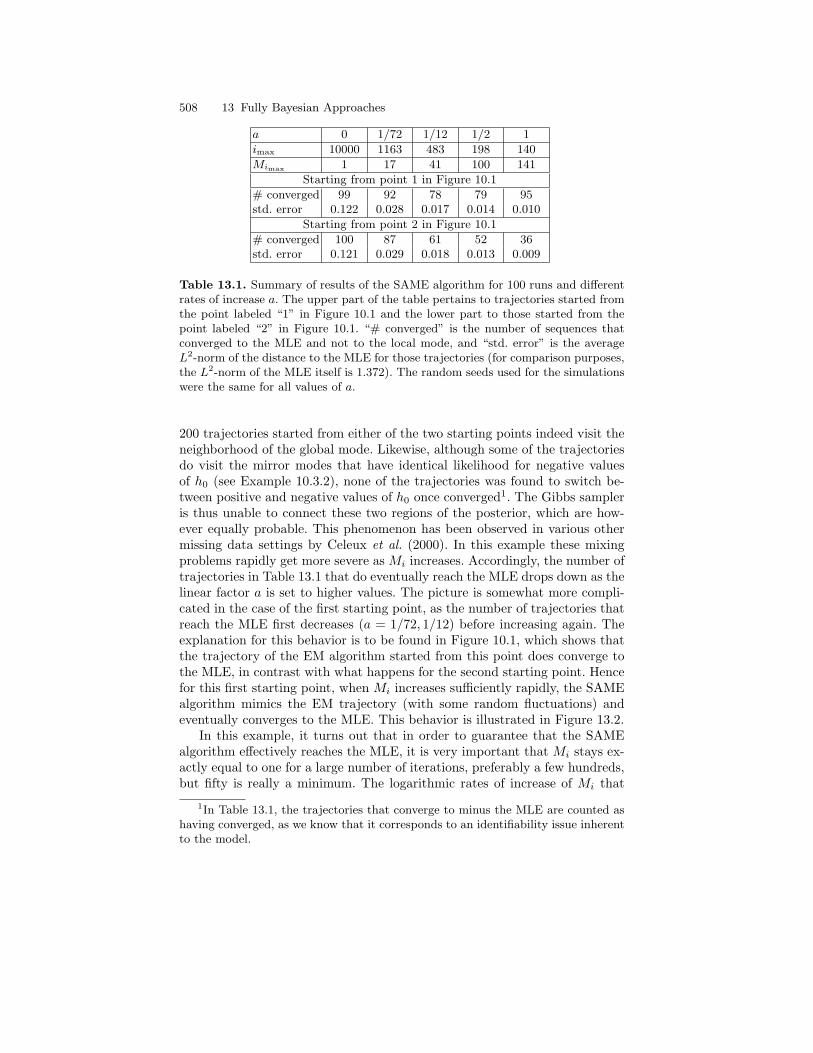
508 13 Fully Bayesian Approaches

a 0 1/72 1/12 1/2 1

imax 10000 1163 483 198 140

Mimax 1 17 41 100 141

Starting from point 1 in Figure 10.1

# converged 99 92 78 79 95std. error 0.122 0.028 0.017 0.014 0.010

Starting from point 2 in Figure 10.1

# converged 100 87 61 52 36std. error 0.121 0.029 0.018 0.013 0.009

Table 13.1. Summary of results of the SAME algorithm for 100 runs and differentrates of increase a. The upper part of the table pertains to trajectories started fromthe point labeled “1” in Figure 10.1 and the lower part to those started from thepoint labeled “2” in Figure 10.1. “# converged” is the number of sequences thatconverged to the MLE and not to the local mode, and “std. error” is the averageL2-norm of the distance to the MLE for those trajectories (for comparison purposes,the L2-norm of the MLE itself is 1.372). The random seeds used for the simulationswere the same for all values of a.

200 trajectories started from either of the two starting points indeed visit theneighborhood of the global mode. Likewise, although some of the trajectoriesdo visit the mirror modes that have identical likelihood for negative valuesof h0 (see Example 10.3.2), none of the trajectories was found to switch be-tween positive and negative values of h0 once converged1. The Gibbs sampleris thus unable to connect these two regions of the posterior, which are how-ever equally probable. This phenomenon has been observed in various othermissing data settings by Celeux et al. (2000). In this example these mixingproblems rapidly get more severe as Mi increases. Accordingly, the number oftrajectories in Table 13.1 that do eventually reach the MLE drops down as thelinear factor a is set to higher values. The picture is somewhat more compli-cated in the case of the first starting point, as the number of trajectories thatreach the MLE first decreases (a = 1/72, 1/12) before increasing again. Theexplanation for this behavior is to be found in Figure 10.1, which shows thatthe trajectory of the EM algorithm started from this point does converge tothe MLE, in contrast with what happens for the second starting point. Hencefor this first starting point, when Mi increases sufficiently rapidly, the SAMEalgorithm mimics the EM trajectory (with some random fluctuations) andeventually converges to the MLE. This behavior is illustrated in Figure 13.2.

In this example, it turns out that in order to guarantee that the SAMEalgorithm effectively reaches the MLE, it is very important that Mi stays ex-actly equal to one for a large number of iterations, preferably a few hundreds,but fifty is really a minimum. The logarithmic rates of increase of Mi that

1In Table 13.1, the trajectories that converge to minus the MLE are counted ashaving converged, as we know that it corresponds to an identifiability issue inherentto the model.

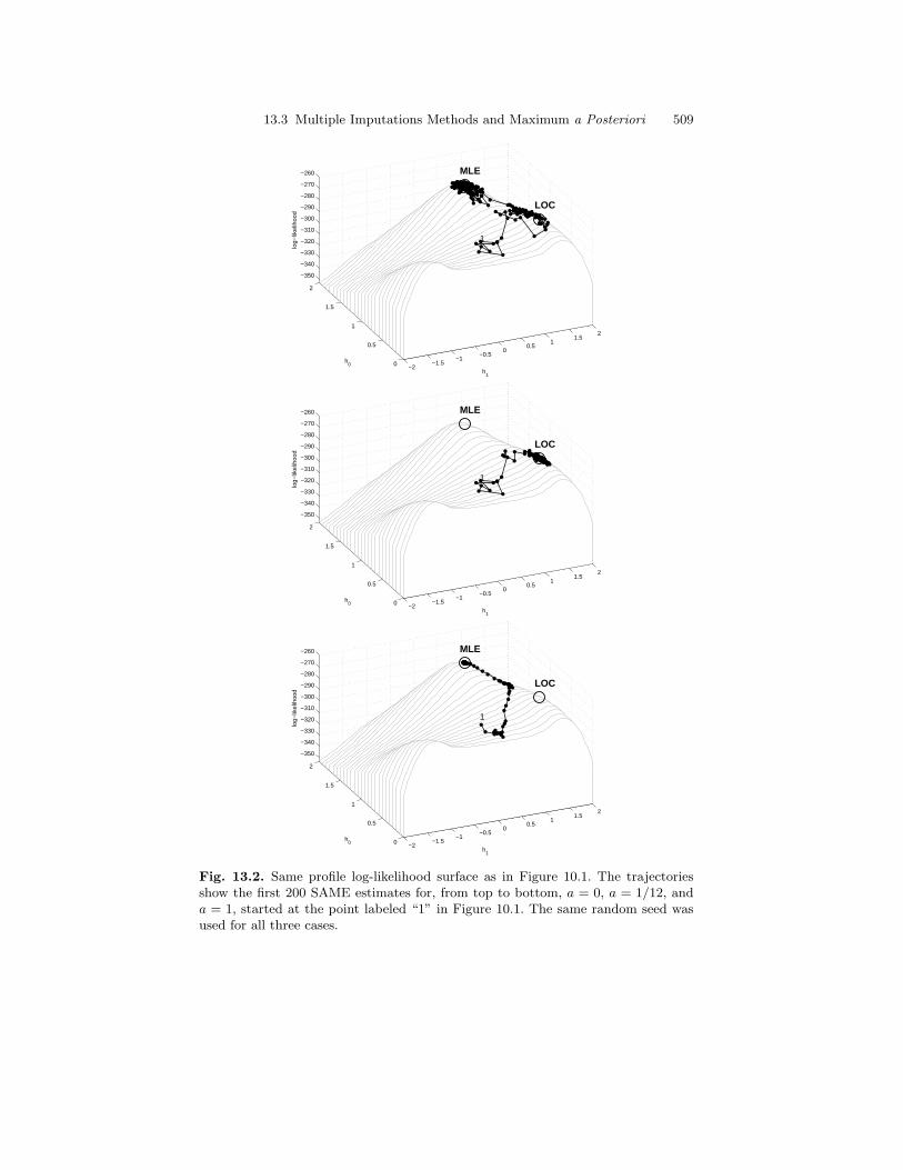
13.3 Multiple Imputations Methods and Maximum a Posteriori 509

−2−1.5

−1−0.5

00.5

11.5

2

0

0.5

1

1.5

2

−350

−340

−330

−320

−310

−300

−290

−280

−270

−260

LOC

h1

1

MLE

h0

log−

likel

ihoo

d

−2−1.5

−1−0.5

00.5

11.5

2

0

0.5

1

1.5

2

−350

−340

−330

−320

−310

−300

−290

−280

−270

−260

LOC

h1

1

MLE

h0

log−

likel

ihoo

d

−2−1.5

−1−0.5

00.5

11.5

2

0

0.5

1

1.5

2

−350

−340

−330

−320

−310

−300

−290

−280

−270

−260

LOC

h1

1

MLE

h0

log−

likel

ihoo

d

Fig. 13.2. Same profile log-likelihood surface as in Figure 10.1. The trajectoriesshow the first 200 SAME estimates for, from top to bottom, a = 0, a = 1/12, anda = 1, started at the point labeled “1” in Figure 10.1. The same random seed wasused for all three cases.

510 13 Fully Bayesian Approaches

are compatible with this constraint and with the objective of using an overallnumber of simulations equal to 10,000 typically end up with Mimax being ofthe order three and are thus roughly equivalent to the MCMC run (a = 0)in Table 13.1. Note that the error obtained with this simple scheme is notthat bad, being about ten times smaller than the L2 norm of the MLE. Thefactor a = 1/72, which gives a reasonable probability of convergence to theMLE from both points, provides an error that is further reduced by a factorof ten.

We would like to point out that—especially when the answer is knownas in this toy example!—it is usually possible to find out by trial-and-errorcooling schedules that are efficient for the problem (data and model) at hand.In the case of Example 13.3.3, setting Mi = 1 for the first 280 iterations andletting Mi = 4, 16, 36, 64, 100 for the last five iterations (500 simulations intotal) is very successful with 98 (resp. 96) trajectories converging to the MLEand an average error of 0.018 (resp. 0.020) when started from the two initialpoints under consideration. The last five iterations in this cooling schedulefollow a square progression that was used for the MCEM algorithm in Exam-ple 11.1.3. Note that rather than freezing the parameter by abruptly increasingMi, one could use instead the averaging strategy (see Section 11.1.2) advo-cated by Gaetan and Yao (2003). Clearly, one-size-fits-all cooling schedulessuch as linear or logarithmic rates of increase may be hard to adjust to a par-ticular problem, at least when the overall number of simulations is limited toa reasonable amount. This observation contrasts with the behavior observedfor the MCEM and SAEM algorithms in Chapter 11, which are more robustin this respect, particularly for the latter. Remember however that we are heretackling a much harder problem in trying not only to avoid all local maximabut also to ensure that the parameter estimate eventually gets reasonablyclose to the actual global maximum.

There is no doubt that simulated annealing strategies in general, andSAME in particular, are very powerful tools for global maximization of thelikelihood or marginal posterior in HMMs. Their usefulness in practical sit-uations however depends crucially on the ability to select proper finite-effortcooling schedules, which may itself be a difficult issue.

Part III

Background and Complements

14

Elements of Markov Chain Theory

14.1 Chains on Countable State Spaces

We review the key elements of the mathematical theory developed for study-ing the limiting behavior of Markov chains. In this first section, we restrictourselves to the case where the state space X is countable, which is conceptu-ally simpler. On our way, we will also meet a number of important conceptsto be used in the next section when dealing with Markov chains on generalstate spaces.

14.1.1 Irreducibility

Let Xkk≥0 be a Markov chain on a countable state space X with transitionmatrix Q. For any x ∈ X, we define the first hitting time σx on x and thereturn time τx to x respectively as

σx = infn ≥ 0 : Xn = x , (14.1)τx = infn ≥ 1 : Xn = x , (14.2)

where, by convention, inf ∅ = +∞. The successive hitting times σ(n)x and

return times τ (n)x , n ≥ 0, are defined inductively by

σ(0)x = 0, σ(1)

x = σx, σ(n+1)x = infk > σ(n)

x : Xk = x ,τ (0)x = 0, τ (1)

x = τx, τ(n+1)x = infk > τ (n)

x : Xk = x .

For two states x and y, we say that state x leads to state y, which we writex→ y, if Px(σy <∞) > 0. In words, x leads to y if the state y can be reachedfrom x. An alternative, equivalent definition is that there exists some integern ≥ 0 such that the n-step transition probability Qn(x, y) > 0. If both x leadsto y and y leads to x, then we say that the x and y communicate, which wewrite x↔ y.

514 14 Elements of Markov Chain Theory

Theorem 14.1.1. The relation “↔” is an equivalence relation on X.

Proof. We need to prove that the relation ↔ is reflexive, symmetric, andtransitive. The first two properties are immediate because, by definition, forall x, y ∈ X, x↔ x (reflexivity), and x↔ y if and only if y ↔ x (symmetry).

For any pairwise distinct x, y, z ∈ X, σy + σz θσy < ∞ ⊂ σz < ∞(if the chain reaches y at some time and later z, it certainly reaches z). Thestrong Markov property (Theorem 2.1.6) implies that

Px(σz <∞) ≥ Px(σy + σz θσy <∞) = Ex[1σy<∞1σz<∞ θσy ]

= Ex[1σy<∞ PXσy (σz <∞)] = Px(σy <∞) Py(σz <∞) .

In words, if the chain can reach y from x and z from y, it can reach z from xby going through y. Hence if x→ y and y → z, then x→ z (transitivity). ut

For x ∈ X, we denote the equivalence class of x with respect to the relation“↔” by C(x). Because “↔” is an equivalence relation, there exists a collectionxi of states, which may be finite or infinite, such that the classes C(xi)form a partition of the state space X.

Definition 14.1.2 (Irreducibility). If C(x) = X for some x ∈ X (and thenfor all x ∈ X), the Markov chain is called irreducible.

14.1.2 Recurrence and Transience

When a state is visited by the Markov chain, it is natural to ask how oftenthe state is visited in the long-run. Define the occupation time of the state xas

ηxdef=

∞∑n=0

1x(Xn) =∞∑j=1

1σ(j)x <∞ .

If the expected number of visits to x starting from x is finite, that is, ifEx[ηx] <∞, then the state x is called transient. Otherwise, if Ex[ηx] =∞, xis said to be recurrent. When X is countable, the recurrence or transience ofa state x can be expressed in terms of the probability Px(τx < ∞) that thechain started in x ever returns to x.

Proposition 14.1.3. For any x ∈ X the following hold true,

(i) If x is recurrent, then Px(ηx =∞) = 1 and Px(τx <∞) = 1.(ii) If x is transient, then Px(ηx <∞) = 1 and Px(τx <∞) < 1.

(iii) Ex[ηx] = 1/[1− Px(τx <∞)], with 1/0 =∞.

Proof. By construction,

Ex[ηx] =∞∑k=1

Px(ηx ≥ k) =∞∑k=1

Px(σ(k)x <∞) .

14.1 Chains on Countable State Spaces 515

Applying strong Markov property (Theorem 2.1.6) for n > 1, we obtain

Px(σ(n)x <∞) = Px(σ(n−1)

x <∞, τx θσ(n−1)x <∞)

= Ex[1σ(n−1)x <∞ PX

σ(n−1)x

(τx <∞)] .

If σ(n−1)x <∞, then X

σ(n−1)x

= x Px-a.s., so that

Px(σ(n)x <∞) = Px(τx <∞) Px(σ(n−1)

x <∞) .

By definition Px(σx < ∞) = 1, whence Px(σ(n)x < ∞) = [Px(τx < ∞)]n−1

and

Ex[ηx] =∞∑n=1

[Px(τx <∞)]n−1 .

This proves part (iii).Now assume x is recurrent. Then by definition Ex[ηx] = ∞, and hence

Px(τx <∞) = 1 and Px(τ (n)x <∞) = 1 for all n ≥ 1. Thus ηx =∞ Px-a.s.

If x is transient then Ex[ηx] <∞, which implies Px(τx <∞) < 1. ut

For a recurrent state x, the occupation time of x is infinite with probabilityone under Px; essentially, once the chain started from x returns to x withprobability one, it returns a second time with probability one, and so on.Thus the occupation time of a state has a remarkable property, not sharedby all random variables: if the expectation of the occupation time is infinite,then the actual number of returns is infinite with probability one. The meanof the occupation time of a state obeys the so-called maximum principle.

Proposition 14.1.4. For all x and y in X,

Ex[ηy] = Px(σy <∞) Ey[ηy] , (14.3)

with the convention 0×∞ = 0.

Proof. It follows from the definition that ηy1σy=∞ = 0 and ηy1σy<∞ =ηy θσy1σy<∞. Thus, applying the strong Markov property,

Ex[ηy] = Ex[1σy<∞ηy] = Ex[1σy<∞ ηy θσy ]

= Ex[1σy<∞ EXσy [ηy]] = Px(σy <∞) Ey[ηy] .

ut

Corollary 14.1.5. If Ex[ηy] = ∞ for some x, then y is recurrent. If X isfinite, then there exists at least one recurrent state.

Proof. By Proposition 14.1.4, Ey[ηy] ≥ Ex[ηy], so that Ex[ηy] = ∞ impliesthat Ey[ηy] =∞, that is, y is recurrent.

Next, obviously∑y∈X ηy = ∞ and thus for all x ∈ X,

∑y∈X Ex[ηy] = ∞.

Hence if X is finite, given x ∈ X there necessarily exists at least one y ∈ Xsuch that Ex[ηy] =∞, which implies that y is recurrent. ut

516 14 Elements of Markov Chain Theory

Our next result shows that a recurrent state can only lead to anotherrecurrent state.

Proposition 14.1.6. Let x be a recurrent state. Then for y ∈ X, either of thefollowing two statements holds true.

(i) x leads to y, Ex[ηy] = ∞, y is recurrent and leads to x, and Px(τy <∞) = Py(τx <∞) = 1;

(ii) x does not lead to y and Ex[ηy] = 0.

Proof. Assume that x leads to y. Then there exists an integer k such thatQk(x, y) > 0. Applying the Chapman-Kolmogorov equations, we obtainQn+k(x, y) ≥ Qn(x, x)Qk(x, y) for all n. Hence

Ex[ηy] ≥∞∑n=1

Qn+k(x, y) ≥∞∑n=1

Qn(x, x)Qk(x, y) = Ex[ηx]Qk(x, y) =∞ .

Thus y is also recurrent by Corollary 14.1.5. Because x is recurrent, the strongMarkov property implies that

0 = Px(τx =∞) ≥ Px(τy <∞, τx =∞)= Px(τy <∞, τx θτy =∞) = Px(τy <∞) Py(τx =∞) .

Because x leads to y, Px(τy <∞) > 0, whence Py(τx =∞) = 0. Thus y leadsto x and moreover Py(τx <∞) = 1. By symmetry, Px(τy <∞) = 1.

If x does not lead to y then Proposition 14.1.4 shows that Ex[ηy] = 0. ut

For a recurrent state x, the equivalence class C(x) (with respect to therelation of communication defined in Section 14.1.1) may thus be equivalentlydefined as

C(x) = y ∈ X : Ex[ηy] =∞ = y ∈ X : Px(τy <∞) = 1 . (14.4)

If y 6∈ C(x), then Px(ηy = 0) = 1, which implies that Px(Xn ∈ C(x) for alln ≥ 0) = 1. In words, the chain started from the recurrent state x foreverstays in C(x) and visits each state of C(x) infinitely many times.

The behavior of a Markov chain can thus be described as follows. If achain is not irreducible, there may exist several equivalence classes of com-munication. Some of them contain only transient states, and some containonly recurrent states. The latter are then called recurrence classes. If a chainstarts from a recurrent state, then it remains in its recurrence class forever.If it starts from a transient state, then either it stays in the class of transientstates forever, which implies that there exist infinitely many transient states,or it reaches a recurrent state and then remains in its recurrence class forever.

In contrast, if the chain is irreducible, then all the states are either transientor recurrent. This is called the solidarity property of an irreducible chain. Wenow summarize the previous results.

14.1 Chains on Countable State Spaces 517

Theorem 14.1.7. Consider an irreducible Markov chain on a countable statespace X. Then every state is either transient, and the chain is called transient,or every state is recurrent, and the chain is called recurrent. Moreover, eitherof the following two statements holds true for all x and y in X.

(i) Px(τy <∞) = 1, Ex[ηy] =∞ and the chain is recurrent.(ii) Px(τx <∞) < 1, Ex[ηy] <∞ and the chain is transient.

Remark 14.1.8. Note that in the transient case, we do not necessarily havePx(τy <∞) < 1 for all x and y in X. For instance, if Q is a transition matrixon N such that Q(n, n+ 1) = 1 for all n, then Pk(τn <∞) = 1 for all k < n.Nevertheless all states are obviously transient because Xn = X0 + n.

14.1.3 Invariant Measures and Stationarity

For many purposes, we might want the marginal distribution of Xk not todepend on k. If this is the case, then by the Markov property it follows thatthe finite-dimensional distributions of Xk are invariant under translation intime, and Xk is thus a stationary process. Such considerations lead us toinvariant distributions. A non-negative vector π(x)x∈X with the property

π(y) =∑x∈X

π(x)Q(x, y) , y ∈ X ,

will be called invariant. If the invariant vector π is summable, then we assumeit is a probability distribution, that is, it sums to one. Such distributions arealso called stationary distributions or stationary probability measures. The keyresult concerning the existence of invariant vectors is the following.

Theorem 14.1.9. Consider an irreducible recurrent Markov chain Xkk≥0

on a countable state space X. Then there exists a unique (up to a scalingfactor) invariant measure π. Moreover 0 < π(x) < ∞ for all x ∈ X. Thismeasure is summable if and only if there exists a state x such that

Ex[τx] <∞ . (14.5)

In this case, Ey[τy] < ∞ for all y ∈ X and the unique invariant probabilitymeasure is given by

π(x) = 1/Ex[τx] , x ∈ X . (14.6)

Proof. Let Q be the transition matrix of the chain. Pick an arbitrary statex ∈ X and define the measure λx by

λx(y) = Ex

[τx−1∑k=0

1y(Xk)

]= Ex

[τx∑k=1

1y(Xk)

]. (14.7)

518 14 Elements of Markov Chain Theory

That is, λx(y) is the expected number of visits to the state y before the firstreturn to x, given that the chain starts in x. Let f be a non-negative functionon X. Then

λx(f) = Ex

[τx−1∑k=0

f(Xk)

]=∞∑k=0

Ex[1τx>kf(Xk)

].

Using this identity and the fact that Qf(Xk) = Ex[f(Xk+1) | FXk ] Px-a.s. forall k ≥ 1, we find that

λx(Qf) =∞∑k=0

Ex[1τx>kQf(Xk)] =∞∑k=0

Ex1τx>k Ex[f(Xk+1) | FXk ]

=∞∑k=0

Ex[1τx>kf(Xk+1)] = Ex

[τx∑k=1

f(Xk)

],

showing that λx(Qf) = λx(f) − f(x) + Ex[f(Xτx)] = λx(f). Because f wasarbitrary, we see that λxQ = λx; the measure λx is invariant. For any otherstate y, the chain may reach y before returning to x when starting in x,as it is irreducible. This proves that λx(y) > 0. Moreover, again by irre-ducibility, we can pick an m > 0 such that Qm(y, x) > 0. By invarianceλx(x) =

∑z∈X λx(z)Qm(z, x) ≥ λx(y)Qm(y, x), and as λx(x) = 1, we see that

λx(y) <∞We now prove that the invariant measure is unique up to a scaling factor.

The first step consists in proving that if π is an invariant measure such thatπ(x) = 1, then π ≥ λx. It suffices to show that, for any y ∈ X and any integern,

π(y) ≥n∑k=1

Ex[1y(Xk)1τx≥k] . (14.8)

The proof is by induction. The inequality is immediate for n = 1. Assumethat (14.8) holds for some n ≥ 1. Then

π(y) = Q(x, y) +∑z 6=x

π(z)Q(z, y)

≥ Q(x, y) +n∑k=1

Ex[Q(Xk, y)1xc(Xk)1τx≥k]

≥ Q(x, y) +n∑k=1

Ex[1y(Xk+1)1τx≥k+1]

=n+1∑k=1

Ex[1y(Xk)1τx≥k] ,

showing the induction. We will now show that π = λx. The proof is by con-tradiction. Assume that π(z) > λx(z) for some z ∈ X. Then

14.1 Chains on Countable State Spaces 519

1 = π(x) = πQ(x) =∑z∈X

π(z)Q(z, x) >∑z∈X

λx(z)Q(z, x) = λx(x) = 1 ,

which cannot be true.The measure λx is summable if and only if

∞ >∑y∈X

λx(y) =∑y∈X

Ex

[τx−1∑k=0

1Xk=y

]= Ex[τx] .

Thus the unique invariant measure is summable if and only if a state xsatisfying this relation exists. On the other hand, if such a state x existsthen, by uniqueness of the invariant measure, Ey[τy] < ∞ must hold forall states y. In this case, the invariant probability measure, π say, satisfiesπ(x) = λx(x)/λx(X) = 1/Ex[τx]. Because the reference state x was in factarbitrary, we find that π(y) = 1/Ex[τy] for all states y. ut

It is natural to ask what can be inferred from the knowledge that a chainpossesses an invariant probability measure. The next proposition gives a par-tial answer.

Proposition 14.1.10. Let Q be a transition matrix and π an invariant prob-ability measure. Then every state x such that π(x) > 0 is recurrent. If Q isirreducible, then it is recurrent.

Proof. Let y ∈ X. If π(y) > 0 then∑∞n=0 πQ

n(y) =∑∞n=0 π(y) =∞. On the

other hand, by Proposition 14.1.4,

∞∑n=0

πQn(y) =∑x∈X

π(x)∞∑n=0

Qn(x, y)

=∑x∈X

π(x) Ex[ηy] ≤ Ey[ηy]∑x∈X

π(x) = Ey[ηy] . (14.9)

Thus π(y) > 0 implies Ey[ηy] =∞, that is, y is recurrent. ut

Let Xk be an irreducible Markov chain. If there exists an invariantprobability measure, the chain is called positive recurrent ; otherwise it is callednull. Note that null chains can be either null recurrent or transient. Transientchains are always null, though they may admit an invariant measure.

14.1.4 Ergodicity

A key result for positive recurrent irreducible chains is that the transition lawsconverge, in a suitable sense, to the invariant vector π. The classical result isthe following.

520 14 Elements of Markov Chain Theory

Proposition 14.1.11. Consider an irreducible and positive recurrent Markovchain on a countable state space. Then for any states x and y,

n−1n∑i=1

Qn(x, y)→ π(y) as n→∞ . (14.10)

The use of the Cesaro limit can be avoided if the chain is aperiodic. Thesimplest definition of aperiodicity is that a state x is aperiodic if Qk(x, x) > 0for all k sufficiently large or, equivalently, that the period of the state x isone. The period of x is defined as the greatest common divisor of the setI(x) = n > 0 : Qn(x, x) > 0. For irreducible chains, the following resultholds true.

Proposition 14.1.12. If the chain is irreducible, then all states have thesame period. If the transition matrix Q is irreducible and aperiodic, then forall x and y in X, there exists n(x, y) ∈ N such that Qk(x, y) > 0 for allk ≥ n(x, y).

Thus, an irreducible chain can be said to be aperiodic if the common periodof all states is one.

The traditional pointwise convergence (14.10) of transition probabilitieshas been replaced in more recent research by convergence in total variation(see Definition 4.3.1). The convergence result may then be formulated as fol-lows.

Theorem 14.1.13. Consider an irreducible and aperiodic positive recurrentMarkov chain on a countable state space X with transition matrix Q and in-variant probability distribution π. Then for all initial distributions ξ and ξ′

on X,‖ξQn − ξ′Qn‖TV → 0 as n→∞ . (14.11)

In particular, for any x ∈ X we may set ξ = δx and ξ′ = π to obtain

‖Qn(x, ·)− π‖TV → 0 as n→∞ . (14.12)

The proof of this result, and indeed the focus on convergence in total variation,follows using of the coupling technique. We postpone the presentation of thistechnique to Section 14.2.4 because essentially the same ideas can be appliedto Markov chains on general state spaces.

14.2 Chains on General State Spaces

In this section, we extend the concepts and results pertaining to countablestate spaces to general ones. In the following, X is an arbitrary set, and wejust require that it is equipped with a countably generated σ-field X . ByXkk≥0 we denote an X-valued Markov chain with transition kernel Q. It

14.2 Chains on General State Spaces 521

is defined on a probability space (Ω,F ,P), and FX = FXk k≥0 denotes thenatural filtration of Xk.

For any set A ∈ X , we define the first hitting time σA and return time τArespectively by

σA = infn ≥ 0 : Xn ∈ A , (14.13)τA = infn ≥ 1 : Xn ∈ A , (14.14)

where, by convention, inf ∅ = +∞. The successive hitting times σ(n)A and

return times τ (n)A , n ≥ 0, are defined inductively by

σ(0)A = 0, σ(1)

A = σA, σ(n+1)A = infk > σ

(n)A : Xk ∈ A ,

τ(0)A = 0, τ (1)

A = τA, τ(n+1)A = infk > τ

(n)A : Xk ∈ A .

We again define the occupation time ηA as the number of visits by Xk toA,

ηAdef=

∞∑k=0

1A(Xk) . (14.15)

14.2.1 Irreducibility

The first step to develop a theory on general state spaces is to define a suitableconcept of irreducibility. The definition of irreducibility adopted for countablestate spaces does not extend to general ones, as the probability of reachingsingle point x in the state space is typically zero.

Definition 14.2.1 (Phi-irreducibility). The transition kernel Q, or theMarkov chain Xkk≥0 with transition kernel Q, is said to be phi-irreducibleif there exists a measure φ on (X,X ) such that for any A ∈ X with φ(A) > 0,Px(τA < ∞) > 0 for all x ∈ X. Such a measure is called an irreducibilitymeasure for Q.

Phi-irreducibility is a weaker property than irreducibility of a transition kernelon a countable state space. If a transition kernel on a countable state spaceis irreducible, then it is phi-irreducible, and any measure is an irreducibilitymeasure. The converse is not true. For instance, the transition kernel

Q =(

0 10 1

)on 0, 1 is phi-irreducible (δ1 is an irreducibility measure for Q) but notirreducible.

In general, there are infinitely many irreducibility measures, and two ir-reducibility measures are not necessarily equivalent. For instance, if φ is anirreducibility measure and φ is absolutely continuous with respect to φ, then

522 14 Elements of Markov Chain Theory

φ is also an irreducibility measure. Nevertheless, as shown in the next re-sult, there exist maximal irreducibility measures ψ, which are such that anyirreducibility measure φ is absolutely continuous with respect to ψ.

Theorem 14.2.2. Let Q be a phi-irreducible transition kernel on (X,X ).Then there exists an irreducibility measure ψ such that all irreducibility mea-sures are absolutely continuous with respect to ψ and for all A ∈ X ,

ψ(A) > 0 ⇔ Px(τA <∞) > 0 for all x ∈ X . (14.16)

Proof. Let φ be an irreducibility measure and ε ∈ (0, 1). Let φε be the measuredefined by φε = φKε, where Kε is the resolvent kernel defined by

Kε(x,A) def= (1− ε)∑k≥0

εkQk(x,A) , x ∈ X, A ∈ X . (14.17)

We will first show that φε is an irreducibility measure. Let A ∈ X be suchthat φε(A) > 0 and define

A = x ∈ X : Px(σA <∞) > 0 = x ∈ X : Kε(x,A) > 0 . (14.18)

By definition, φε(A) > 0 implies that φ(A) > 0. Define Am = x ∈ X :Px(σA < ∞) ≥ 1/m. By construction, A =

⋃m>0 Am, and because φ(A) >

0, there exists m such that φ(Am) > 0. Because φ is an irreducibility measure,Px(τAm <∞) > 0 for all x ∈ X. Hence by the strong Markov property, for allx ∈ X,

Px(τA <∞) ≥ Px(τAm + σA θτAm <∞ , τAm <∞)

= Ex[1τAm<∞ PXτAm (σA <∞)] ≥ 1m

Px(τAm <∞) > 0 ,

showing that φε is an irreducibility measure.Now for m ≥ 0 the Chapman-Kolmogorov equations imply∫

X

φε(dx) εmQm(x,A) = (1− ε)∫

X

∞∑n=m

εnQn(x,A)φ(dx) ≤ φε(A) .

Therefore, if φε(A) = 0 then φεKε(A) = 0, which in turn implies φε(A) = 0.Summarizing the results above, for any A ∈ X ,

φε(A) > 0⇔ φε (x ∈ X : Px(σA <∞) > 0) > 0 . (14.19)

This proves (14.16)To conclude we must show that all irreducibility measures are absolutely

continuous with respect to φε. Let φ be an irreducibility measure and let C ∈X be such that φ(C) > 0. Then φε (x ∈ X : Px(σC <∞) > 0) = φε(X) >0, which, by (14.19), implies that φε(C) > 0 . This exactly says that φ isabsolutely continuous with respect to φε. ut

14.2 Chains on General State Spaces 523

A set A ∈ X is said to be accessible for the kernel Q (or Q-accessible,or simply accessible if there is no risk of confusion) if Px(τA < ∞) > 0 forall x ∈ X. The family of accessible sets is denoted X+. If ψ is a maximalirreducibility measure the set A is accessible if and only if ψ(A) > 0.

Example 14.2.3 (Autoregressive Model). The first-order autoregressivemodel on R is defined iteratively by Xn = φXn−1 + Un, where φ is a realnumber and Un is an i.i.d. sequence. If Γ is the probability distributionof the noise sequence Un, the transition kernel of this chain is given byQ(x,A) = Γ (A − φx). The autoregressive model is phi-irreducible providedthat the noise distribution has an everywhere positive density with respect toLebesgue measure λLeb. If we take φ = λLeb, it is easy to see that wheneverλLeb(A) > 0, we have Γ (A − φx) > 0 for any x, and so Q(x,A) > 0 in justone step.

Example 14.2.4. The Metropolis-Hastings algorithm, introduced in Chap-ter 6, provides another typical example of a general state-space Markov chain.For simplicity, we assume here that X = Rd, which we equip with the Borelσ-field X = B(Rd). Assume that we are given a probability density functionπ on with respect to Lebesgue measure λLeb. Let r be a transition densitykernel. Starting from Xn = x, a candidate transition x′ is generated fromr(x, ·) and accepted with probability

α(x, x′) =π(x′) r(x′, x)π(x) r(x, x′)

∧ 1 . (14.20)

The transition kernel of the Metropolis-Hastings chain is given by

Q(x,A) =∫A

α(x, x′)r(x, x′)λLeb(dx′)

+ 1x(A)∫

[1− α(x, x′)]r(x, x′)λLeb(dx′) . (14.21)

There are various sufficient conditions for the Metropolis-Hastings algorithmto be phi-irreducible (Roberts and Tweedie, 1996; Mengersen and Tweedie,1996). For the Metropolis-Hastings chain, it is simple to check that the chainis phi-irreducible if for λLeb-almost all x′ ∈ X, the condition π(x′) > 0 impliesthat r(x, x′) > 0 for any x ∈ X.

14.2.2 Recurrence and Transience

In view of the discussion above, it is not sensible to define recurrence andtransience in terms of the expectation of the occupation measure of a state, butfor phi-irreducible chains it makes sense to consider the occupation measureof accessible sets.

524 14 Elements of Markov Chain Theory

Definition 14.2.5 (Uniform Transience and Recurrence). A set A ∈ Xis called uniformly transient if supx∈A Ex[ηA] < ∞. A set A ∈ X is calledrecurrent if Ex[ηA] = +∞ for all x ∈ A.

Obviously, if supx∈X Ex[ηA] < ∞, then A is uniformly transient. In fact thereverse implication holds true too, because if the chain is started outside A itcannot hit Amore times, on average, than if it is started at “the most favorablelocation” in A. Thus an alternative definition of a uniformly transient set issupx∈X Ex[ηA] <∞.

The main result on phi-irreducible transition kernels is the following re-currence/transience dichotomy, which parallels Theorem 14.1.7 for countablestate-space Markov chains.

Theorem 14.2.6. Let Q be a phi-irreducible transition kernel (or Markovchain). Then either of the following two statements holds true.

(i) Every accessible set is recurrent, in which case we call Q recurrent.(ii) There is a countable cover of X with uniformly transient sets, in which

case we call Q transient.

In the next section, we will prove Theorem 14.2.6 in the particular casewhere the chain possesses an accessible atom (see Definition 14.2.7); the proofis then very similar to that for countable state space. In the general case,the proof is more involved. It is necessary to introduce small sets and the so-called splitting construction, which relates the chain to one that does possessan accessible atom.

14.2.2.1 Transience and Recurrence for Chains Possessing anAccessible Atom

Definition 14.2.7 (Atom). A set α ∈ X is called an atom if there exists aprobability measure ν on (X,X ) such that Q(x,A) = ν(A) for all x ∈ α andA ∈ X .

Atoms behave the same way as do individual states in the countable statespace case. Although any singleton x is an atom, it is not necessarily ac-cessible, so that Markov chain theory on general state spaces differs from thetheory of countable state space chains.

If α is an atom for Q, then for any m ≥ 1 it is an atom for Qm. Thereforewe denote by Qm(α, ·) the common value of Qm(x, ·) for all x ∈ α. Thisimplies that if the chain starts from within the atom, the distribution of thewhole chain does not depend on the precise starting point. Therefore we willalso use the notation Pα instead of Px for any x ∈ α.

Example 14.2.8 (Random Walk on the Half-Line). The random walkon the half-line (RWHL) is defined by an initial condition X0 ≥ 0 and therecursion

14.2 Chains on General State Spaces 525

Xk+1 = (Xk +Wk+1)+ , k ≥ 0 , (14.22)

where Wkk≥1 is an i.i.d. sequence of random variables, independent of X0,with distribution function Γ on R. This process is a Markov chain with tran-sition kernel Q defined by

Q(x,A) = Γ (A− x) + Γ ((−∞ ,−x])1A(0) , x ∈ R+, A ∈ B(R+) ,

where A− x = y− x : y ∈ A. The set 0 is an atom, and it is accessible ifand only if Γ ((−∞ , 0]) > 0.

We now prove Theorem 14.2.6 when there exists an accessible atom.

Proposition 14.2.9. Let Xkk≥0 be a Markov chain that possesses an ac-cessible atom α, with associated probability measure ν. Then the chain is phi-irreducible, ν is an irreducibility measure, and a set A ∈ X is accessible if andonly if Pα(τA <∞) > 0.

Moreover, α is recurrent if and only if Pα(τα < ∞) = 1 and (uniformly)transient otherwise, and the chain is recurrent if α is recurrent and transientotherwise.

Proof. For all A ∈ X and x ∈ X, the strong Markov property yields

Px(τA <∞) ≥ Px(τα + τA θτα <∞, τα <∞)= Ex[PXτα (τA <∞)1τα<∞]= Pα(τA <∞) Px(τα <∞)≥ ν(A) Px(τα <∞) .

Because α is accessible, Px(τα < ∞) > 0 for all x ∈ X. Thus for any A ∈ Xsatisfying ν(A) > 0, it holds that Px(τA < ∞) > 0 for all x ∈ X, showingthat ν is an irreducibility measure. The above display also shows that A isaccessible if and only if Pα(τA <∞).

Now let σ(n)α be the successive hitting times of α (see (14.13)). The strong

Markov property implies that for any n > 1,

Pα(σ(n)α <∞) = Pα(τα <∞) Pα(σ(n−1)

α <∞) .

Hence, as for discrete state spaces, Pα(σ(n)α < ∞) = [Pα(τα < ∞)]n−1 and

Eα[ηα] = 1/[1 − Pα(τα < ∞)]. This proves that α is recurrent if and only ifPα(τα <∞) = 1.

Assume that α is recurrent. Because the atom α is accessible, for anyx ∈ X, there exists r such that Qr(x, α) > 0. If A ∈ X+ there exists s suchthat Qs(α,A) > 0. By the Chapman-Kolmogorov equations,

∑n≥1

Qr+s+n(x,A) ≥ Qr(x, α)

∑n≥1

Qn(α, α)

Qs(α,A) =∞ .

526 14 Elements of Markov Chain Theory

Hence Ex[ηA] = ∞ for all x ∈ X and A is recurrent. Because A was anarbitrary accessible set, the chain is recurrent.

Assume now that α is transient, in which case Eα(ηα) < ∞. Then, fol-lowing the same line of reasoning as in the discrete state space case (proof ofProposition 14.1.4), we obtain that for all x ∈ X,

Ex[ηα] = Px(τα <∞) Eα[ηα] ≤ Eα[ηα] . (14.23)

Define Bj = x :∑jn=1Q

n(x, α) ≥ 1/j. Then ∪∞j=1Bj = X because α is ac-cessible. Applying the definition of the sets Bj and the Chapman-Kolmogorovequations, we find that

∞∑k=1

Qk(x,Bj) ≤∞∑k=1

Qk(x,Bj) infy∈Bj

j

j∑`=1

Q`(y, α)

≤ j∞∑k=1

j∑`=1

∫Bj

Qk(x, dy)Q`(y, α) ≤ j2∞∑k=1

Qk(x, α) = j2 Ex[ηα] <∞ .

The sets Bj are thus uniformly transient. The proof is complete. ut

14.2.2.2 Small Sets and the Splitting Construction

We now return to the general phi-irreducible case. In order to prove Theo-rem 14.2.6, we need to introduce the splitting technique. To do so, we needto define a class of sets (containing accessible sets) that behave the same wayin many respects as do atoms. We shall see this in many of the results below,which exactly mimic the atomic case results they generalize. These sets arecalled small sets.

Definition 14.2.10 (Small Set). Let Q and ν be a transition kernel and aprobability measure, respectively, on (X,X ), let m be a positive integer andε ∈ (0, 1]. A set C ∈ X is called a (m, ε, ν)-small set for Q, or simply a smallset, if ν(C) > 0 and for all x ∈ C and A ∈ X ,

Qm(x,A) ≥ εν(A) .

If ε = 1 then C is an atom for the kernel Qm.

Trivially, any individual point is a small set, but small sets that are notaccessible are of limited interest. If the state space is countable and Q isirreducible, then every finite set is small. The minorization measure associatedto an accessible small set provides an irreducibility measure.

Proposition 14.2.11. Let C be an accessible (m, ε, ν)-small set for the tran-sition kernel Q on (X,X ). Then ν is an irreducibility measure.

14.2 Chains on General State Spaces 527

Proof. Let A ∈ X be such that ν(A) > 0. The strong Markov property yields

Px(τA <∞) ≥ Px(τC <∞, τA θτC <∞) = Ex[1τC<∞ PXτC (τA <∞)] .

Because C is a small set, for all y ∈ C it holds that

Py(τA <∞) ≥ Py(Xm ∈ A) = Qm(y,A) ≥ εν(A) .

Because C is accessible and ν(A) > 0, for all x ∈ X it holds that

Px(τA <∞) ≥ εν(A) Px(τC <∞) > 0 .

Thus A is accessible, whence ν is an irreducibility measure. ut

An important result due to Jain and Jamison (1967) states that if thetransition kernel is phi-irreducible, then small sets do exist. For a proof seeNummelin (1984, p. 16) or Meyn and Tweedie (1993, Theorem 5.2.2).

Proposition 14.2.12. If the transition kernel Q on (X,X ) is phi-irreducible,then every accessible set contains an accessible small set.

Given the existence of just one small set from Proposition 14.2.12, we mayshow that it is possible to cover X with a countable number of small sets inthe phi-irreducible case.

Proposition 14.2.13. Let Q be a phi-irreducible transition kernel on (X,X ).

(i) If C ∈ X is an (m, ε, ν)-small set and for any x ∈ D we have Qn(x,C) ≥δ, then D is (m+ n, δε, ν)-small set.

(ii) If Q is phi-irreducible then there exists a countable collection of smallsets Ci such that X =

⋃i Ci.

Proof. Using the Chapman-Kolmogorov equations, we find that for any x ∈ D,

Qn+m(x,A) ≥∫C

Qn(x, dy)Qm(y,A) ≥ εQn(x,C)ν(A) ≥ εδν(A) ,

showing part (i). Because Q is phi-irreducible, by Proposition 14.2.12 thereexists an accessible (m, ε, ν)-small set C. Moreover, by the definition of phi-irreducibility, the sets C(n,m) = x : Qn(x,C) ≥ 1/m cover X and, bypart (i), each C(n,m) is small. ut

Proposition 14.2.14. If Q is phi-irreducible and transient, then every acces-sible small set is uniformly transient.

Proof. Let C be an accessible (m, ε, ν)-small set. If Q is transient, there ex-ists at least one A ∈ X+ that is uniformly transient. For δ ∈ (0, 1), by theChapman-Kolmogorov equations,

528 14 Elements of Markov Chain Theory

Ex[ηA] =∞∑k=0

Qk(x,A) ≥ (1− δ)∞∑p=0

δp∞∑k=0

Qk+m+p(x,A)

≥ (1− δ)∞∑p=0

δp∞∑k=0

∫C

Qk(x, dx′)∫Qm(x′, dx′′)Qp(x′′, A)

≥ ε∞∑k=0

Qk(x,C)× (1− δ)∞∑p=0

δpνQp(A) = εEx[ηC ] νKδ(A) ,

where Kδ is the resolvent kernel (14.17). Because C is an accessible smallset, Proposition 14.2.11 shows that ν is an irreducibility measure. By The-orem 14.2.2, νKδ is a maximal irreducibility measure, so that νKδ(A) > 0.Thus supx∈X Ex[ηC ] <∞ and we conclude that C is uniformly transient (seethe remark following Definition 14.2.5). ut

Example 14.2.15 (Autoregressive Process, Continued). Suppose thatthe noise distribution in Example 14.2.3 has an everywhere positive continuousdensity γ with respect to Lebesgue measure λLeb. If C = [−M,M ] and ε =inf |x|≤(1+φ)M γ(u), then for A ⊆ C,

Q(x,A) =∫A

γ(x′ − φx) dx′ ≥ ελLeb(A) .

Hence the compact set C is small. Obviously R is covered by a countable col-lection of small sets and every accessible set (here sets with non-zero Lebesguemeasure) contains a small set.

Example 14.2.16 (Metropolis-Hastings Algorithm, Continued). Sim-ilar results hold for the Metropolis-Hastings algorithm of Example 14.2.4 ifπ(x) and r(x, x′) are positive and continuous for all (x, x′) ∈ X × X. Sup-pose that C is compact with λLeb(C) > 0. By positivity and continuity, wethen have d = supx∈C π(x) < ∞ and ε = inf(x,x′)∈C×C q(x, x′) > 0. For anyA ⊆ C, define

Rx(A) def=x′ ∈ A :

π(x′)q(x′, x)π(x)q(x, x′)

< 1,

the region of possible rejection. Then for any x ∈ C,

Q(x,A) ≥∫A

q(x, x′)α(x, x′) dx′

≥∫Rx(A)

q(x′, x)π(x)

π(x′) dx′ +∫A\Rx(A)

q(x, x′) dx′

≥ ε

d

∫Rx(A)

π(x′) dx′ +ε

d

∫A\Rx(A)

π(x′) dx′

=ε

d

∫A

π(x′) dx′ .

14.2 Chains on General State Spaces 529

Thus C is small and, again, X can be covered by a countable collection ofsmall sets.

We now show that it is possible to define a Markov chain with an atom,the so-called split chain, whose properties are directly related to those of theoriginal chain. This technique was introduced by Nummelin (1978) (Athreyaand Ney, 1978, introduced, independently, a virtually identical concept) andallows extending results valid for Markov chain possessing an accessible atomto irreducible Markov chains that only possess small sets. The basic idea isas follows. Suppose the chain admits a (1, ε, ν)-small set C. Then as long asthe chain does not enter C, the transition kernel Q is used to generate thetrajectory. However, as soon as the chain hits C, say Xn ∈ C, a zero-onerandom variable dn is drawn, independent of everything else. The probabilitythat dn = 1 is ε, and hence dn = 0 with probability 1− ε. Then if dn = 1, thenext value Xn+1 is drawn from ν; otherwise Xn+1 is drawn from the kernel

R(x,A) = [1− ε1C(x)]−1[Q(x,A)− ε1C(x)ν(A)] ,

with x = Xn. It is immediate that εν(A) + (1 − ε)R(x,A) = Q(x,A) for allx ∈ C, so Xn+1 is indeed drawn from the correct (conditional) distribution.Note also that R(x, ·) = Q(x, ·) for x 6∈ C. So, what is gained by this approach?What is gained is that whenever Xn ∈ C and dn = 1, the next value of thechain will be independent of Xn (because it is drawn from ν). This is oftencalled a regeneration time, as the joint chain (Xk, dk) in a sense “restarts”and forgets its history. In technical terms, the state C × 1 in the extendedstate space is as atom, and it will be accessible provided C is.

We now make this formal. Thus we define the so-called extended state spaceas X = X × 0, 1 and let X be the associated product σ-field. We associateto every measure µ on (X,X ) the split measure µ? on (X, X ) as the uniquemeasure satisfying, for A ∈ X ,

µ?(A× 0) = (1− ε)µ(A ∩ C) + µ(A ∩ Cc) ,µ?(A× 1) = εµ(A ∩ C) .

If Q is a transition kernel on (X,X ), we define the kernel Q? on X × X byQ?(x, A) = [Q(x, ·)]?(A) for x ∈ X and A ∈ X .

Assume now that Q is a phi-irreducible transition kernel and let C be a(1, ε, ν)-small set. We define the split transition kernel Q on X×X as follows.For any x ∈ X and A ∈ X ,

Q((x, 0), A) = R?(x, A) , (14.24)

Q((x, 1), A) = ν?(A) . (14.25)

Examining the above technicalities, we find that transitions into Cc×1have zero probability from everywhere, so that dn = 1 can only occur ifXn ∈ C. Because dn = 1 indicates a regeneration time, from within C, this is

530 14 Elements of Markov Chain Theory

logical. Likewise we find that given a transition to some y ∈ C, the conditionalprobability that dn = 1 is ε, wherever the transition took place from. Thus theabove split transition kernel corresponds to the following simulation schemefor (Xk, dk). Assume (Xk, dk) are given. If Xk 6∈ C, then draw Xk+1 fromQ(Xk, ·). If Xk ∈ C and dn = 1, then draw Xk+1 from ν, otherwise fromR(Xk, ·). If the realized Xk+1 is not in C, then set dk+1 = 0; if Xk+1 is in C,then set dk+1 = 1 with probability ε, and otherwise set dk+1 = 0.

Split measures operate on the split kernel in the following way. For anymeasure µ on (X,X ),

µ?Q = (µQ)?. (14.26)

For any probability measure µ on X , we denote by Pµ and Eµ, respectively, theprobability distribution and the expectation on the canonical space (XN, X⊗N)such that the coordinate process, denoted (Xk, dk)k≥0, is a Markov chainwith initial probability measure µ and transition kernel Q. We also denote byFkk≥0 the natural filtration of this chain and, as usual, by FXk k≥0 thenatural filtration of Xkk≥0.

Proposition 14.2.17. Let Q be a phi-irreducible transition kernel on (X,X ),let C be an accessible (1, ε, ν)-small set for Q and let µ be a probability measureon (X,X ). Then for any bounded X -measurable function f and any k ≥ 1,

Eµ? [f(Xk) | FXk−1] = Qf(Xk−1) Pµ?-a.s. (14.27)

Before giving the proof, we discuss the implications of this result. It impliesthat under Pµ? , Xkk≥0 is a Markov chain (with respect to its natural filtra-tion) with transition kernel Q and initial distribution µ. By abuse of notation,we can identify Xk with the coordinate process associated to the canoni-cal space XN. Denote by Pµ the probability measure on (XN,X⊗N) such thatXkk≥0 is a Markov chain with transition kernel Q and initial distributionµ (see Section 2.1.2.1) and denote by Eµ the associated expectation opera-tor. Then Proposition 14.2.17 yields the following identity. For any boundedFX∞-measurable random variable Y ,

Eµ? [Y ] = Eµ[Y ] . (14.28)

Proof (of Proposition 14.2.17). We have, µ?-a.s.,

Eµ? [f(Xk) | Fk−1] = 1dk−1=1ν(f) + 1dk−1=0Rf(Xk−1) .

Because Pµ(dk−1 = 1 | FXk−1) = ε1C(Xk−1) Pµ? -a.s., it holds that

Eµ? [f(Xk) | FXk−1] = Eµ?E[f(Xk) | Fk−1] | FXk−1= ε1C(Xk−1)ν(f) + [1− ε1C(Xk−1)]Rf(Xk−1)= Qf(Xk−1) .

ut

14.2 Chains on General State Spaces 531

Corollary 14.2.18. Under the assumptions of Proposition 14.2.17, X × 1is an accessible atom and ν? is an irreducibility measure for the split kernelQ. More generally, if B ∈ X is accessible for Q, then B × 0, 1 is accessiblefor the split kernel.

Proof. Because α = X × 1 is an atom for the split kernel Q, Proposi-tion 14.2.9 shows that ν? is an irreducibility measure if α is accessible. Ap-plying (14.28) we obtain for x ∈ X,

P(x,1)(τα <∞) = P(x,1)(dn = 1 for some n ≥ 1)

≥ P(x,1)(d1 = 1) = εν(C) > 0 ,

P(x,0)(τα <∞) = P(x,0)((Xn, dn) ∈ C × 1 for some n ≥ 1)

≥ P(x,0)(τC×0,1 <∞ , dτC×0,1 = 1) = εPx(τC <∞) > 0 .

Thus α is accessible and ν? is an irreducibility measure for Q. This implies, byTheorem 14.2.2, that for all η ∈ (0, 1), ν?Kη is a maximal irreducibility mea-sure for the split kernel Q; here Kη is the resolvent kernel (14.17) associatedto Q. By straightforward applications of the definitions, it is easy to checkthat ν?Kη = (νKη)?. Moreover, ν is an irreducibility measure for Q, and νKη

is a maximal irreducibility measure for Q (still by Proposition 14.2.11 andTheorem 14.2.2). If B is accessible, then νKη(B) > 0 and

ν?Kη(B × 0, 1) = (νKη)?(B × 0, 1) = νKη(B) > 0.

Thus B × 0, 1 is accessible for Q. ut

14.2.2.3 Transience/Recurrence Dichotomy for GeneralPhi-irreducible Chains

Using the splitting construction, we are now able to prove Theorem 14.2.6 forchains not possessing accessible atoms. We first consider the simple case inwhich the chain possesses a 1-small set.

Proposition 14.2.19. Let Q be a phi-irreducible transition kernel that admitsan accessible (1, ε, ν)-small set C. Then Q is either recurrent or transient. Itis recurrent if and only if the small set C is recurrent.

Proof. Because the split chain possesses an accessible atom, by Proposi-tion 14.2.9 the split chain is phi-irreducible and either recurrent or transient.Applying (14.28) we can write

Eδ?x [ηB×0,1] = Ex[ηB ] . (14.29)

Assume first that the split chain is recurrent. Let B be an accessible set forQ. By Proposition 14.2.17, B × 0, 1 is accessible for the split chain. Hence

532 14 Elements of Markov Chain Theory

Eδ?x [ηB×0,1] = ∞ for all x ∈ B, so that, by (14.29), Ex[ηB ] = ∞ for allx ∈ B.

Conversely, if the split chain is transient, then by Proposition 14.2.9 theatom α is transient. For j ≥ 1, define Bj = x :

∑jl=1 Q

l((x, 0), α) ≥ 1/j.Because α is accessible, ∪∞j=1Bj = X. By the same argument as in the proofof Proposition 14.2.9, the sets Bj ×0, 1 are uniformly transient for the splitchain. Hence, by (14.29), the sets Bj are uniformly transient for Q.

It remains to prove that if the small set C is recurrent, then the chain isrecurrent. We have just proved that Q is recurrent if and only if Q is recurrentand, by Proposition 14.2.9, this is true if and only if the atom α is recurrent.Thus we only need to prove that if C is recurrent then α is recurrent. If C isrecurrent, then (14.29) yields for all x ∈ C,

Eδ?x [ηα] ≥ εEδ?x [ηC×0,1] = εEx[ηC ] =∞ .

Using the definition of δ?x, this implies that there exists x ∈ X such thatEx[ηα] = ∞. This observation and (14.23) imply that Eα[ηα] = ∞, that is,the atom is recurrent. ut

Using the resolvent kernel, the previous results can be extended to thegeneral case where an accessible small set exists, but not necessarily a 1-smallone.

Proposition 14.2.20. Let Q be transition kernel.

(i) If Q is phi-irreducible and admits an accessible (m, ε, ν)-small set C, thenfor any η ∈ (0, 1), C is an accessible (1, ε′, ν)-small set for the resolventkernel Kη = (1− η)

∑∞k=0 η

kQk with ε′ = (1− η)ηmε.(ii) A set is recurrent (resp. uniformly transient) for Q if and only if it is

recurrent (resp. uniformly transient) for Kη for some (hence for all)η ∈ (0, 1).

(iii) Q is recurrent (resp. transient) if and only if Kη is recurrent (resp. tran-sient) for some (hence for all) η ∈ (0, 1).

Proof. For any η > 0, x ∈ C, and A ∈ X ,

Kη(x,A) ≥ (1− η)ηmQm(x,A) ≥ (1− η)ηmεν(A) = ε′ν(A) .

Thus C is a (1, ε′, ν)-small set for Kη, showing part (i). The remaining claimsfollow from the identity ∑

n≥1

Knη =

1− ηη

∑n≥0

Qn .

ut

14.2 Chains on General State Spaces 533

14.2.2.4 Harris Recurrence

As for countable state spaces, it is sometimes useful to consider stronger recur-rence properties, expressed in terms of return probabilities rather than meanoccupation times.

Definition 14.2.21 (Harris Recurrence). A set A ∈ X is said to be Harrisrecurrent if Px(τA < ∞) = 1 for any x ∈ X. A phi-irreducible Markov chainis said to be Harris (recurrent) if any accessible set is Harris recurrent.

It is intuitively obvious that, as for countable state spaces, Harris recur-rence implies recurrence.

Proposition 14.2.22. A Harris recurrent set is recurrent.

Proof. Let A be a Harris recurrent set. Because for j ≥ 1, σ(j+1)A = τA θσ

(j)A

on the set σ(j)A <∞, the strong Markov property implies that for any x ∈ A,

Px(σ(j+1)A <∞) = Ex

[PX

σ(j)A

(τA <∞)1σ(j)A <∞

]= Px(σ(j)

A <∞) .

Because Px(σ(1)A < ∞) = 1 for x ∈ A, we obtain that for all x ∈ A and all

j ≥ 1, Px(σ(j)A = 1) and Ex[ηA] =

∑∞j=1 Px(σ(j)

A <∞) =∞. ut

Even though all transition kernels may not be Harris recurrent, the fol-lowing theorem provides a very useful decomposition of the state space of arecurrent phi-irreducible transition kernel. For a proof of this result, see Meynand Tweedie (1993, Theorem 9.1.5)

Theorem 14.2.23. Let Q be a phi-irreducible recurrent transition kernel ona state space X and let ψ be a maximal irreducibility measure. Then X = N∪H,where N is covered by a countable family of uniformly transient sets, ψ(N) = 0and every accessible subset of H is Harris recurrent.

As a consequence, if A is an accessible set of a recurrent phi-irreducible chain,then there exists a set A′ ⊆ A such that ψ(A \ A′) = 0 for any maximalirreducibility measure ψ, and Px(τA′ <∞) = 1 for all x ∈ A′.

Example 14.2.24. To understand why a recurrent Markov chain can fail tobe Harris, consider the following elementary example of a chain on X = N. Letthe transition kernel Q be given by Q(0, 0) = 1 and for x ≥ 1, Q(x, x+1) = 1−1/x2 and Q(x, 0) = 1/x2. Thus the state 0 is absorbing. Because Q(x, 0) > 0for any x ∈ X, δ0 is an irreducibility measure. In fact, by application ofTheorem 14.2.2, this measure is maximal. The set 0 is an atom and becauseP0(τ0 <∞) = 1, the chain is recurrent by Proposition 14.2.9.

The chain is not Harris recurrent, however. Indeed, for any x ≥ 1 we have

534 14 Elements of Markov Chain Theory

Px(τ0 ≥ k) = Px(X1 6= 0, . . . , Xk−1 6= 0) =x+k−1∏j=x

(1− 1/j2) .

Because∏∞j=2(1− 1/j2) > 0, we obtain that Px(τ0 =∞) = limk→∞ Px(τ0 ≥

k) > 0 for any x ≥ 2, so that the accessible state 0 is not certainly reachedfrom such an initial state. Comparing to Theorem 14.2.23, we see that thedecomposition of the state space is given by H = 0 and N = 1, 2, . . ..

14.2.3 Invariant Measures and Stationarity

On general state spaces, we again further classify chains using invariant mea-sures. A σ-finite measure µ is called Q-sub-invariant if µ ≥ µQ and Q-invariant if µ = µQ.

Theorem 14.2.25. A phi-irreducible recurrent transition kernel (or Markovchain) admits a unique (up to a multiplicative constant) invariant measurewhich is also a maximal irreducibility measure.

This result leads us to define the following classes of chains.

Definition 14.2.26 (Positive and Null Chains). A phi-irreducible tran-sition kernel (or Markov chain) is called positive if it admits an invariantprobability measure; otherwise it is called null.

We now prove the existence of an invariant measure when the chain admitsan accessible atom. The invariant measure is defined as for countable statespaces, by replacing an individual state by the atom. Thus define the measureµα on X by

µα(A) = Eα

[τα∑n=1

1A(Xn)

], A ∈ X . (14.30)

Proposition 14.2.27. Let α be an accessible atom for the transition kernelQ. Then µα is Q-sub-invariant. It is invariant if and only if the atom α isrecurrent. In that case, any Q-invariant measure µ is proportional to µα, andµα is a maximal irreducibility measure.

Proof. By the definition of µα and the strong Markov property,

µαQ(A) = Eα

[τα∑k=1

Q(Xk, A)

]= Eα

[τα+1∑k=2

1A(Xk)

]= µα(A)− Pα(X1 ∈ A) + Eα[1A(Xτα+1)1τα<∞] .

Applying the strong Markov property once again yields

14.2 Chains on General State Spaces 535

Eα[1A(Xτα+1)1τα<∞] = EαEα[1A(X1) θτα | FXτα ]1τα<∞= Eα[PXτα (X1 ∈ A)1τα<∞] = Pα(X1 ∈ A) Pα(τα <∞) .

Thus µαQ(A) = µα(A)− Pα(X1 ∈ A)[1− Pα(τα <∞)]. This proves that µαis sub-invariant, and invariant if and only if Pα(τα <∞) = 1.

Now let µ be an invariant non-trivial measure and let A be an accessible setsuch that µ(A) <∞. Then there exists an integer n such that Qn(α,A) > 0.Because µ is invariant, it holds that µ = µQn, so that

∞ > µ(A) = µQn(A) ≥ µ(α)Qn(α,A) .

This implies that µ(α) <∞. Without loss of generality, we can assume µ(α) >0; otherwise we replace µ by µ+µα. Assuming µ(α) > 0, there is then no lossof generality in assuming µ(α) = 1.

The next step is to prove that if µ is an invariant measure such thatµ(α) = 1, then µ ≥ µα. To prove this it suffices to prove that for all n ≥ 1,

µ(A) ≥n∑k=1

Pα(Xk ∈ A, τα ≥ k) .

We prove this inequality by induction. For n = 1 we can write

µ(A) = µQ(A) ≥ µ(α)Q(α,A) = Q(α,A) = Pα(X1 ∈ A) .

Now assume now that the inequality holds for some n ≥ 1. Then

µ(A) = Q(α,A) +∫αcµ(dy)Q(y,A)

≥ Q(α,A) +n∑k=1

Eα[Q(Xk, A)1τα≥k1Xk /∈α]

≥ Q(α,A) +n∑k=1

Eα[Q(Xk, A)1τα≥k+1] .

Because τα ≥ k + 1 ∈ FXk , the Markov property yields

Eα[Q(Xk, A)1τα≥k+1] = Pα(Xk+1 ∈ A, τα ≥ k + 1) ,

whence

µ(A) ≥ Q(α,A) +n+1∑k=2

Pα(Xk ∈ A, τα ≥ k) =n+1∑k=1

Pα(Xk ∈ A, τα ≥ k) .

This completes the induction, and we conclude that µ ≥ µα.Assume that there exists a set A such that µ(A) > µα(A). It is straight-

forward that µ and µα are both invariant for the resolvent kernel Kδ (see

536 14 Elements of Markov Chain Theory

(14.17)), for any δ ∈ (0, 1). Because α is accessible, Kδ(x, α) > 0 for all x ∈ X.Hence

∫Aµ(dx)Q(x, α) >

∫Aµα(dx)Q(x, α), which implies that

1 = µ(α) = µKδ(α) =∫A

µ(dx)Kδ(x, α) +∫Acµ(dx)Kδ(x, α)

>

∫A

µα(dx)Kδ(x, α) +∫Acµα(dx)Kδ(x, α) = µαKδ(α) = µα(α) = 1.

This contradiction shows that µ = µα.We finally prove that µα is a maximal irreducibility measure. Let ψ be a

maximal irreducibility measure and assume that ψ(A) = 0. Then Px(τA <∞) = 0 for ψ-almost all x ∈ X. This obviously implies that Px(τA < ∞) = 0for ψ-almost all x ∈ α. Because Px(τA < ∞) is constant over α, we findthat Px(τA < ∞) = 0 for all x ∈ α, and this yields µα(A) = 0. Thus µαis absolutely continuous with respect to ψ, hence an irreducibility measure.Let again Kδ be the resolvent kernel. By Theorem 14.2.2, µαKδ is a maximalirreducibility measure. But, as noted above, µαKε = µα, and therefore µα isa maximal irreducibility measure. ut

Proposition 14.2.28. Let Q be a recurrent phi-irreducible transition kernelthat admits an accessible (1, ε, ν)-small set C. Then it admits a non-trivialinvariant measure, unique up to multiplication by a constant and such that 0 <π(C) <∞, and any invariant measure is a maximal irreducibility measure.

Proof. By (14.26), (µQ)? = µ?Q, so that µ is Q-invariant if and only if µ? isQ-invariant. Let µ be a Q-invariant measure and define

µ =∫C×0

µ(dx)R(x, ·) +∫Cc×0

µ(dx)Q(x, ·) + µ(X× 1)ν .

By application of the definition of the split kernel and measures, it can bechecked that µQ = µ?. Hence µ? = µQ = µ. We thus see that µ? is Q-invariant, which, as noted above, implies that µ is Q-invariant. Hence we haveshown that there exists a Q-invariant measure if and only if there exists aQ-invariant one.

If Q is recurrent then C is recurrent, and as appears in the proof of Propo-sition 14.2.28 this implies that the atom α is recurrent for the split chainQ. Thus, by Proposition 14.2.9 the kernel Q is recurrent, and by Proposi-tion 14.2.27 it admits an invariant measure that is unique up to a scalingfactor. Hence Q also admits an invariant measure, unique up to a scalingfactor and such that 0 < π(C) <∞.

Let µ be Q-invariant. Then µ? is Q-invariant and hence, by Proposi-tion 14.2.27, a maximal irreducibility measure. If µ(A) > 0, then µ?(A ×0, 1) = µ(A) > 0. Thus A × 0, 1 is accessible, and this implies that A isaccessible. We conclude that µ is an irreducibility measure, and it is maximalbecause it is Kη-invariant. ut

14.2 Chains on General State Spaces 537

If the kernelQ is phi-irreducible and admits an accessible (m, ε, ν)-small setC, then, by Proposition 14.2.20, for any η ∈ (0, 1) the set C is an accessible(1, ε′, ν)-small set for the resolvent kernel Kη. If C is recurrent for Q, it isalso recurrent for Kη and therefore, by Proposition 14.2.19, Kη has a uniqueinvariant probability measure. The following result shows that this probabilitymeasure is invariant also for Q.

Lemma 14.2.29. A measure µ on (X,X ) is Q-invariant if and only if µ isKη-invariant for some (hence for all) η ∈ (0, 1).

Proof. If µQ = µ, then obviously µQn = µ for all n ≥ 0, so that µKη = µ.Conversely, assume that µKη = µ. Because Kη = ηQKη + (1 − η)Q0 andQKη = KηQ, it holds that

µ = µKη = ηµQKη + (1− η)µ = ηµKηQ+ (1− η)µ = ηµQ+ (1− η)µ .

Hence ηµQ = ηµ, which concludes the proof. ut

14.2.3.1 Drift Conditions

We first give a sufficient condition for a chain to be positive, based on theexpectation of the return time to an accessible small set.

Proposition 14.2.30. Let Q be a transition kernel that admits an accessiblesmall set C such that

supx∈C

Ex[τC ] <∞ . (14.31)

Then the chain is positive and the invariant probability measure π satisfies,for all A ∈ X ,

π(A) =∫C

π(dy) Ey

[τC−1∑k=0

1A(Xk)

]=∫C

π(dy) Ey

[τC∑k=1

1A(Xk)

]. (14.32)

If f is a non-negative measurable function such that

supx∈C

Ex

[τC−1∑k=0

f(Xk)

]<∞ , (14.33)

then f is integrable with respect to π and

π(f) =∫C

π(dy) Ey

[τC−1∑k=0

f(Xk)

]=∫C

π(dy) Ey

[τC∑k=1

f(Xk)

].

538 14 Elements of Markov Chain Theory

Proof. First note that by Proposition 14.2.11, Q is phi-irreducible. Equa-tion (14.31) implies that for all Px(τC <∞) = 1 x ∈ C, that is, C is Harris re-current. By Proposition 14.2.22, C is recurrent, and so, by Proposition 14.2.19,Q is recurrent. Let π be an invariant measure such that 0 < π(C) < ∞, theexistence of which is given by Proposition 14.2.28. Then define a measure µCon X by

µC(A) def=∫C

π(dy) Ey

[τC∑k=1

1A(Xk)

].

Because τC < ∞ Py-a.s. for all y ∈ C, it holds that µC(C) = π(C). Thenwe can show that µC(A) = π(A) for all A ∈ X . The proof is along the samelines as the proof of Proposition 14.2.27 and is therefore omitted. Thus, µC isinvariant. In addition, we obtain that for any measurable set A,∫

C

π(dy) Ey [1A(X0)] = π(A ∩ C) = µC(A ∩ C) =∫C

π(dy) Ey [1A(XτC )] ,

and this yields

µC(A) =∫C

π(dy) Ey

[τC∑k=1

1A(Xk)

]=∫C

π(dy) Ey

[τC−1∑k=0

1A(Xk)

].

We thus obtain the following equivalent expressions for µC :

µC(A) =∫C

π(dy) Ey

[τC−1∑k=0

1A(Xk)

]=∫C

µC(dy) Ey

[τC−1∑k=0

1A(Xk)

]

=∫C

µC(dy) Ey

[τC∑k=1

1A(Xk)

]=∫C

π(dy) Ey

[τC∑k=1

1A(Xk)

]= π(A) .

Hence

π(X) =∫C

π(dy) Ey

[τC−1∑k=0

1X(Xk)

]≤ π(C) sup

y∈CEy[τC ] <∞ ,

so that any invariant measure is finite and the chain is positive. Finally, under(14.33) we obtain that

π(f) =∫C

π(dy) Ey

[τC−1∑k=0

f(Xk)

]≤ π(C) sup

y∈CEy

[τC−1∑k=1

f(Xk)

]<∞ .

ut

Except in specific examples (where, for example, the invariant distributionis known in advance), it may be difficult to decide if a chain is positive or null.To check such properties, it is convenient to use drift conditions.

14.2 Chains on General State Spaces 539

Proposition 14.2.31. Assume that there exists a set C ∈ X , two measurablefunctions 1 ≤ f ≤ V , and a constant b > 0 such that

QV ≤ V − f + b1C . (14.34)

Then

Ex[τC ] ≤ V (x) + b1C(x) , (14.35)

Ex [V (XτC )] + Ex

[τC−1∑k=0

f(Xk)

]≤ V (x) + b1C(x) . (14.36)

If C is an accessible small set and V is bounded on C, then the chain ispositive recurrent and π(f) <∞.

Proof. Set for n ≥ 1,

Mn =

[V (Xn) +

n−1∑k=0

f(Xk)

]1τC≥n .

Then

E[Mn+1 | Fn] =

[QV (Xn) +

n∑k=0

f(Xk)

]1τC≥n+1

≤

[V (Xn)− f(Xn) + b1C(Xn) +

n∑k=0

f(Xk)

]1τC≥n+1

=

[V (Xn) +

n−1∑k=0

f(Xk)

]1τC≥n+1 ≤Mn ,

as 1C(Xn)1τC≥n+1 = 0. Hence Mnn≥1 is a non-negative super-martingale.For any integer n, τC ∧ n is a bounded stopping time, and Doob’s optionalstopping theorem shows that for any x ∈ X,

Ex [MτC∧n] ≤ Ex [M1] ≤ V (x) + b1C(x) . (14.37)

Applying this relation with f ≡ 1 yields for any x ∈ X and n ≥ 0,

Ex [τC ∧ n] ≤ V (x) + b1C(x) ,

and (14.35) follows using monotone convergence. This implies in particularthat Px(τC < ∞) = 1 for any x ∈ X. The proof of (14.36) follows similarlyfrom (14.37) by the letting n→∞ and π(f) is finite by (14.33). ut

Example 14.2.32 (Random Walk on the Half-Line, Continued). Con-sider again the model of Example 14.2.8. Previously we have seen that sets ofthe form [0, c] are small. If Γ ((−∞ ,−c]) > 0, then for x ∈ [0, c],

540 14 Elements of Markov Chain Theory

Q(x,A) ≥ Γ ((−∞ ,−c])1A(0) ;

otherwise there exists an integer m such that Γ ∗m((−∞ ,−c]) > 0, whence

Qm(x,A) ≥ Γ ∗m((−∞ ,−c])1A(0) .

To prove recurrence for µ < 0, we apply Proposition 14.2.31. Becauseµ < 0, there exists c > 0 such that

∫∞−c wΓ (dw) ≤ µ/2 < 0. Thus taking

V (x) = x for x > c,

QV (x)− V (x) =∫ ∞−∞

[(x+ w)+ − x]Γ (dw)

= −xΓ ((−∞ ,−x]) +∫ ∞−x

wΓ (dw) ≤ µ/2 .

Hence the chain is positive recurrent.Consider now the case µ > 0. In view of Proposition 14.2.9, we have to

show that the atom 0 is transient. For any n, Xn ≥ X0 +∑ni=1Wi. Define

Cn =∣∣n−1

∑ni=1Wi − µ

∣∣ ≥ µ/2 and write Dn for Xn = 0. The stronglaw of large numbers implies that P0(Dn i.o.) ≤ P0(Cn i.o.) = 0. Hence theatom 0 is transient, and so is the chain.

When µ = 0, additional assumptions on Γ are needed to prove the recur-rence of the RWHL (see for instance Meyn and Tweedie, 1993, Lemma 8.5.2).

Example 14.2.33 (Autoregressive Model, Continued). Consider againthe model of Example 14.2.3 and assume that the noise process has zero meanand finite variance. Choosing V (x) = x2 we have

PV (x) = E[(φx+ U1)2] = φ2V (x) + E[U21 ] ,

so that (14.34) holds when C = [−M,M ] for some large enough M , provided|φ| < 1. Because we know that every compact set is small if the noise processhas an everywhere continuous positive density, Proposition 14.2.31 shows thatthe chain is positive recurrent. Note that this approach provides an existenceresult but does not help us to determine π. If Uk are Gaussian with zeromean and variance σ2, then one can check that the invariant distribution alsois Gaussian with zero mean and variance σ2/(1− φ2).

Theorem 14.2.25 shows that if a chain is phi-irreducible and recurrentthen the chain is positive, that is, it admits a unique invariant probabilitymeasure π. In certain situations, and in particular when dealing with MCMCprocedures, it is known that Q admits an invariant probability measure, but itis not known, a priori, that the chain is recurrent. The following result showsthat positivity implies recurrence.

Proposition 14.2.34. If the Markov kernel Q is positive, then it is recurrent.

14.2 Chains on General State Spaces 541

Proof. Suppose that the chain is positive and let π be an invariant probabilitymeasure. If Q is transient, the state space X is covered by a countable familyAj of uniformly transient subsets (see Theorem 14.2.6). For any j and k,

kπ(Aj) =k∑

n=1

πQn(Aj) ≤∫π(dx) Ex[ηAj ] ≤ sup

x∈XEx[ηAj ] . (14.38)

The strong Markov property implies that

Ex[ηAj ] = Ex[ηAj1σAj<∞]

≤ Ex1σAj<∞ EXσAj [ηAj ] ≤ supx∈Aj

Ex[ηAj ] Px(σAj <∞) .

Thus, the left-hand side of (14.38) is bounded as k → ∞. This implies thatπ(Aj) = 0, and hence π(X) = 0. This is a contradiction so the chain cannotbe transient. ut

14.2.4 Ergodicity

In this section, we study the convergence of iterates Qn of the transitionkernel to the invariant distribution. As for discrete state spaces case, we firstneed to avoid periodic behavior that prevents the iterates to converge. Inthe discrete case, the period of a state x is defined as the greatest commondivisor of the set of time points n ≥ 0 : Qn(x, x) > 0. Of course thisnotion does not extend to general state spaces, but for phi-irreducible chainswe may define the period of accessible small sets. More precisely, let Q be aphi-irreducible transition kernel with maximal irreducibility measure ψ. ByTheorem 14.2.11, there exists an accessible (m, ε, ψ)-small set C. Because ψis a maximal irreducibility measure, ψ(C) > 0, so that when the chain startsfrom C there is a positive probability that the it will return to C at time m.Let

ECdef= n ≥ 1 : the set C is (n, εn, ψ)-small for some εn > 0 (14.39)

be the set of time points for which C is small with minorizing measure ψ.Note that for n and m in EC , B ∈ X+ and x ∈ C,

Qn+m(x,B) ≥∫C

Qm(x, dx′)Qn(x′, B) ≥ εmεnψ(C)ψ(B) > 0 ,

showing that EC is closed under addition. There is thus a natural period forEC , given by the greatest common divisor. Similar to the discrete case (seeProposition 14.1.12), this period d may be shown to be independent of theparticular choice of the small set C (see for instance Meyn and Tweedie, 1993,Theorem 5.4.4).

542 14 Elements of Markov Chain Theory

Proposition 14.2.35. Suppose that Q is phi-irreducible with maximal irre-ducibility measure ψ. Let C be an accessible (m, ε, ψ)-small set and let d be thegreatest common divisor of the set EC , defined in (14.39). Then there existdisjoint sets D1, . . . , Dd (a d-cycle) such that

(i) for x ∈ Di, Q(x,Di+1) = 1, i = 0, . . . , d− 1 (mod d);(ii) the set N = (∪di=1Di)c is ψ-null.

The d-cycle is maximal in the sense if D′1, . . . , D′d′ is a d′-cycle, then d′ divides

d, and if d = d′, then up to a permutation of indices D′i and Di are ψ-almostequal.

It is obvious from the this theorem that the period d does not dependon the choice of the small set C and that any small set must be contained(up to ψ-null sets) inside one specific member of a d-cycle. This in particularimplies that if there exists an accessible (1, ε, ψ)-small set C, then d = 1. Thissuggests the following definition

Definition 14.2.36 (Aperiodicity). Suppose that Q is a phi-irreducibletransition kernel with maximal irreducibility measure ψ. The largest d forwhich a d-cycle exists is called the period of Q. When d = 1, the chain iscalled aperiodic. When there exists a (1, ε, ψ)-small set C, the chain is calledstrongly aperiodic.

In all the examples considered above, we have shown the existence of a1-small set; therefore all these Markov chains are strongly aperiodic.

Now we can state the main convergence result, formulated and proved byAthreya et al. (1996). It parallels Theorem 14.1.13.

Theorem 14.2.37. Let Q be a phi-irreducible positive aperiodic transitionkernel. Then for π-almost all x,

limn→∞

‖Qn(x, ·)− π‖TV = 0 . (14.40)

If Q is Harris recurrent, the convergence occurs for all x ∈ X.

Although this result does not provide information on the rate of conver-gence to the invariant distribution, its assumptions are quite minimal. In fact,it may be shown that these assumptions are essentially necessary and suf-ficient. If ‖Qn(x, ·)− π‖TV → 0 for any x ∈ X, then by Nummelin (1984,Proposition 6.3), the chain is π-irreducible, aperiodic, positive Harris, and πis an invariant distribution. This form of the ergodicity theorem is of particu-lar interest in cases where the invariant distribution is explicitly known, as inMarkov chain Monte Carlo. It provides conditions that are simple and easyto verify, and under which an MCMC algorithm converges to its stationarydistribution.

Of course the exceptional null set for non-Harris recurrent chain is a nui-sance. The example below however shows that there is no way of getting ridof it.

14.2 Chains on General State Spaces 543

Example 14.2.38. In the model of Example 14.2.24, π = δ0 is an invari-ant probability measure. Because Qn(x, 0) = Px(τ0 ≤ n) for any n ≥ 0,limn→∞Qn(x, 0) = Px(τ0 <∞). We have previously shown that Px(τ0 <∞) = 1 − Px(τ0 = ∞) < 1 for x ≥ 2, whence lim sup ‖Qn(x, ·)− π‖TV 6= 0for such x.

Fortunately, in many cases it is not hard to show that a chain is Harris.A proof of Theorem 14.2.37 from first principles is given by Athreya et al.

(1996). We give here a proof due to Rosenthal (1995), based on pathwisecoupling (see Rosenthal, 2001; Roberts and Rosenthal, 2004). The same con-struction is used to compute bounds on ‖Qn(x, ·)− π‖TV. Before provingthe theorem, we briefly introduce the pathwise coupling construction for phi-irreducible Markov chains and present the associated Lindvall inequalities.

14.2.4.1 Pathwise Coupling and Coupling Inequalities

Suppose that we have two probability measures ξ and ξ′ on (X,X ) that aresuch that 1

2 ‖ξ − ξ′‖TV ≤ 1− ε for some ε ∈ (0, 1] or, equivalently (see (4.19)),

that there exists a probability measure ν such that εν ≤ ξ∧ ξ′. Because ξ andξ′ are probability measures, we may construct a probability space (Ω,F ,P)and X-valued random variables X and X ′ such that P(X ∈ ·) = ξ(·) andP(X ′ ∈ ·) = ξ′, respectively. By definition, for any A ∈ X ,

|ξ(A)− ξ′(A)| = |P(X ∈ A)− P(X ′ ∈ A)| = |E[1A(X)− 1A(X ′)]| (14.41)= |E[(1A(X)− 1A(X ′))1X 6=X′]| ≤ P(X 6= X ′) , (14.42)

so that the total variation distance between the laws of two random elements isbounded by the probability that they are unequal. Of course, this inequalityis not in general sharp, but we can construct on an appropriately definedprobability space (Ω, F , P) two X-valued random variables X and X ′ withlaws ξ and ξ′ such that P(X = X ′) ≥ 1− ε. The construction goes as follows.We draw a Bernoulli random variable d with probability of success ε. If d = 0,we then draw X and X ′ independently from the distributions (1−ε)−1 (ξ − εν)and (1 − ε)−1 (ξ′ − εν), respectively. If d = 1, we draw X from ν and setX = X ′. Note that for any A ∈ X ,

P(X ∈ A) = P(X ∈ A | d = 0)P(d = 0) + P(X ∈ A | d = 1)P(d = 1)

= (1− ε)(1− ε)−1[ξ(A)− εν(A)] = ξ(A)

and, similarly, P(X ′ ∈ A) = ξ′(A). Thus, marginally the random variablesX and X ′ are distributed according to ξ and ξ′. By construction, P(X =X ′) ≥ P(d = 1) ≥ ε, showing that X and X ′ are equal with probability atleast ε. Therefore the coupling bound (14.41) can be made sharp by using anappropriate construction. Note that this construction may be used to derivebounds on distances between probability measures that generalize the totalvariation; we will consider in the sequel the V -total variation.

544 14 Elements of Markov Chain Theory

Definition 14.2.39 (V-Total Variation). Let V : X→ [1,∞) be a measur-able function. The V -total variation distance between two probability measuresξ and ξ′ on (X,X ) is

‖ξ − ξ′‖Vdef= sup|f |≤V

|ξ(f)− ξ′(f)| .

If V ≡ 1, ‖ · ‖1 is the total variation distance.

When applied to Markov chains, the whole idea of coupling is to constructon an appropriately defined probability space two Markov chains Xk andX ′k with transition kernel Q and initial distributions ξ and ξ′, respectively,in such a way that Xn = X ′n for all indices n after a random time T , referredto as the coupling time. The coupling procedure attempts to couple the twoMarkov chains when they simultaneously enter a coupling set.

Definition 14.2.40 (Coupling Set). Let C ⊆ X × X, ε ∈ (0, 1] and letν = νx,x′ , x, x′ ∈ X be transition kernels from C (endowed with the traceσ-field) to (X,X ). The set C is a (1, ε,ν)-coupling set if for all (x, x′) ∈ Cand all A ∈ X ,

Q(x,A) ∧Q(x′, A) ≥ ε νx,x′(A) . (14.43)

By applying Lemma 4.3.5, this condition can be stated equivalently as:there exists ε ∈ (0, 1] such that for all (x, x′) ∈ C,

12‖Q(x, ·)−Q(x′, ·)‖TV ≤ 1− ε . (14.44)

For simplicity, only one-step minorization is considered in this chapter.Adaptations to m-step minorization (replacing Q by Qm in (14.43)) can becarried out as in Rosenthal (1995). Condition (14.43) is often satisfied bysetting C = C × C for a (1, ε, ν)-small set C. Indeed, in that case, for all(x, x′) ∈ C × C and A ∈ X ,

Q(x,A) ∧Q(x′, A) ≥ εν(A) .

The case ε = 1 needs some consideration. If there exists an atom, sayα, i.e., there exists a probability measure ν such that for all x ∈ α andA ∈ X , Q(x,A) = ν(A), then C = α × α is a (1, 1,ν)-coupling set withνx,x′ = ν for all (x, x′) ∈ C. Conversely, assume that C is a (1, 1,ν)-couplingset. The alternative characterization (14.44) shows that Q(x, ·) = Q(x′, ·) forall (x, x′) ∈ C, that is, C is an atom. This also implies that the set C containsa set α1 × α2, where α1 and α2 are atoms for Q.

We now introduce the coupling construction. Let C be a (1, ε,ν)-couplingset. Define X = X×X and X = X ⊗X . Let Q be a transition kernel on (X, X )given for all A and A′ in X by

14.2 Chains on General State Spaces 545

Q(x, x′;A×A′) = Q(x,A)Q(x′, A′)1Cc(x, x′)+

(1− ε)−2[Q(x,A)− ενx,x′(A)][Q(x′, A′)− ενx,x′(A′)]1C(x, x′) (14.45)

if ε < 1 and Q = Q ⊗ Q if ε = 1. For any probability measure µ on (X, X ),let Pµ be the probability measure on the canonical space (XN, XN) such thatthe coordinate process Xk is a Markov chain with respect to its naturalfiltration and with initial distribution µ and transition kernel Q. As usual,denote the associated expectation operator by Eµ.

We now define a transition kernel Q on the space X def= X × X × 0, 1endowed with the product σ-field X by, for any x, x′ ∈ X and A,A′ ∈ X ,

Q ((x, x′, 0), A×A′ × 0) = [1− ε1C(x, x′)]Q((x, x′), A×A′) , (14.46)

Q ((x, x′, 0), A×A′ × 1) = ε1C(x, x′)νx,x′(A ∩A′) , (14.47)

Q ((x, x′, 1), A×A′ × 1) = Q(x,A ∩A′) . (14.48)

For any probability measure µ on (X, X ), let Pµ be the probability measureon the canonical space (XN, X⊗N) such that the coordinate process Xk is aMarkov chain with transition kernel Q and initial distribution µ. The corre-sponding expectation operator is denoted by Eµ.

The transition kernel Q can be described algorithmically. Given X0 =(X0, X

′0, d0) = (x, x′, d), X1 = (X1, X

′1, d1) is obtained as follows.

• If d = 1, then draw X1 from Q(x, ·) and set X ′1 = X1, d1 = 1.• If d = 0 and (x, x′) ∈ C, flip a coin with probability of heads ε.

– If the coin comes up heads, draw X1 from νx,x′ and set X ′1 = X1 andd1 = 1.

– If the coin comes up tails, draw (X1, X′1) from Q(x, x′; ·) and set d1 = 0.

• If d = 0 and (x, x′) 6∈ C, draw (X1, X′1) from Q(x, x′; ·) and set d1 = 0.

The variable dn is called the bell variable; it indicates whether coupling hasoccurred by time n (dn = 1) or not (dn = 0). The first index n at whichdn = 1 is the coupling time;

T = infk ≥ 1 : dk = 1.

If dn = 1, then Xk = X ′k for all k ≥ n. The coupling construction is carriedout in such a way that under Pξ⊗ξ′⊗δ0 , Xk and X ′k are Markov chainswith transition kernel Q with initial distributions ξ and ξ′, respectively.

The coupling construction allows deriving quantitative bounds on the(V -)total variation distance in terms of the tail probability of the couplingtime.

Proposition 14.2.41. Assume that the transition kernel Q admits a (1, ε,ν)-coupling set. Then for any probability measures ξ and ξ′ on (X,X ) and anymeasurable function V : X→ [1,∞),

546 14 Elements of Markov Chain Theory

‖ξQn − ξ′Qn‖TV ≤ 2Pξ⊗ξ′⊗δ0(T > n) , (14.49)

‖ξQn − ξ′Qn‖V ≤ 2Eξ⊗ξ′⊗δ0 [V (Xn, X′n)1T>n] , (14.50)

where V : X× X→ [1,∞) is defined by V (x, x′) = V (x) + V (x′)/2.

Proof. We only need to prove (14.50) because (14.49) is obtained by set-ting V ≡ 1. Pick a function f such that |f | ≤ V and note that [f(Xn) −f(X ′n)]1dn=1 = 0. Hence

|ξQnf − ξ′Qnf | = |Eξ⊗ξ′⊗δ0 [f(Xn)− f(X ′n)]|= |Eξ⊗ξ′⊗δ0 [(f(Xn)− f(X ′n))1dn=0]|≤ 2Eξ⊗ξ′⊗δ0 [V (Xn, X

′n)1dn=0] .

utWe now provide an alternative expression of the coupling inequality that

only involves the process Xk. Let σC be the hitting time on the couplingset C by this process, define K0(ε) = 1, and for all n ≥ 1,

Kn(ε) =

1σC≥n if ε = 1 ;∏n−1j=0 [1− ε1C(Xj)] if ε ∈ (0, 1) .

(14.51)

Proposition 14.2.42. Assume that the transition kernel Q admits a (1, ε,ν)-coupling set. Let ξ and ξ′ be probability measures on (X,X ) and let V : X →[1,∞) be a measurable function. Then

‖ξQn − ξ′Qn‖V ≤ 2Eξ⊗ξ′ [V (Xn, X′n)Kn(ε)] , (14.52)

with V (x, x′) = [V (x) + V (x′)]/2.

Proof. We show that for any probability measure µ on (X, X ),

Eµ⊗δ0 [V (Xn, X′n)1T>n] = Eµ[V (Xn, X

′n)Kn(ε)] .

To do this, we shall prove by induction that for any n ≥ 0 and any boundedX -measurable functions fjj≥0,

Eµ⊗δ0

n∏j=0

fj(Xj , X′j)1T>n

= Eµ

n∏j=0

fj(Xj , Xj)Kn(ε)

. (14.53)

This is obviously true for n = 0. For n ≥ 0, put χn =∏nj=0 fj(Xj , X

′j). The

induction assumption and the identity T > n+ 1 = dn+1 = 0 yield

Eµ⊗δ0 [χn+11T>n+1] = Eµ⊗δ0 [χn fn+1(Xn+1, X′n+1)1dn+1=0]

= Eµ⊗δ0χn E[fn+1(Xn+1, X′n+1)1dn+1=0 | Fn]1dn=0

= Eµ⊗δ0χn[1− ε1C(Xn, X′n)]Qfn+1(Xn, X

′n)1dn=0

= Eµ[χnQfn+1(Xn)Kn+1(ε)] = Eµ[χn+1Kn+1(ε)] .

This concludes the induction and the proof. ut

14.2 Chains on General State Spaces 547

14.2.4.2 Proof of Theorem 14.2.37

We preface the proof of Theorem 14.2.37 by two technical lemmas that estab-lish some elementary properties of a chain on the product space with transitionkernel Q⊗Q.

Lemma 14.2.43. Suppose that Q is a phi-irreducible aperiodic transition ker-nel. Then for any n, Qn is phi-irreducible and aperiodic.

Proof. Propositions 14.2.11 and 14.2.12 show that there exists an accessible(m, ε, ν)-small set C and that ν is an irreducibility measure. Because Q isaperiodic, there exists a sequence εk of positive numbers and an integer nCsuch that for all n ≥ nC , x ∈ C, and A ∈ X , Qn(x,A) ≥ εnν(A). In addition,because C is accessible, there exists p such that Qp(x,C) > 0 for any x ∈ X.Therefore for any n ≥ nC and any A ∈ X such that ν(A) > 0,

Qn+p(x,A) ≥∫C

Qp(x, dx′)Qn(x′, A) ≥ εnν(A)Qp(x,C) > 0 . (14.54)

ut

Lemma 14.2.44. Let Q be an aperiodic positive transition kernel with in-variant probability measure π. Then Q⊗Q is phi-irreducible, π⊗ π is Q⊗Q-invariant, and Q ⊗ Q is positive. If C is an accessible (m, ε, ν)-small set forQ, then C × C is an accessible (m, ε2, ν ⊗ ν)-small set for Q⊗Q.

Proof. Because Q is phi-irreducible and admits π as an invariant probabilitymeasure, π is a maximal irreducibility measure for Q. Let C be an accessible(m, ε, ν)-small set for Q. Then for (x, x′) ∈ C × C and A ∈ X ⊗ X ,

(Q⊗Q)m(x, x′;A) =∫∫

A

Qm(x, dy)Qm(x′, dy′) ≥ ε2ν ⊗ ν(A) .

Because ν⊗ ν(C ×C) = [ν(C)]2 > 0, this shows that C ×C is a (1, ε2, ν⊗ ν)-small set for Q ⊗ Q. By (14.54) there exists an integer nx such that for anyn ≥ nx, Qn(x,C) > 0. This implies that for any (x, x′) ∈ X × X and anyn ≥ nx ∨ nx′ ,

(Q⊗Q)n(x, x′ ;C × C) = Qn(x,C)Qn(x′, C) > 0 ,

showing that C × C is accessible. Because C × C is a small set, Proposi-tion 14.2.11 shows that Q⊗Q is phi-irreducible. In addition, π⊗π is invariantfor Q ⊗ Q, so that π ⊗ π is a maximal irreducibility measure and Q ⊗ Q ispositive. ut

We have now all the necessary ingredients to prove Theorem 14.2.37.

548 14 Elements of Markov Chain Theory

Proof (of Theorem 14.2.37). By Lemma 14.2.43, Qm is phi-irreducible for anyinteger m. By Proposition 14.2.12, there exists an accessible (m, ε, ν)-small setC with ν(C) > 0. Lemma 4.3.8 shows that for all integers n,

‖Qn(x, ·)−Qn(x′, ·)‖TV ≤ ‖Qm[n/m](x, ·)−Qm[n/m](x′, ·)‖TV .

Hence it suffices to prove that (14.40) holds for Qm and we may thus withoutloss of generality assume that m = 1.

For any probability measure µ on (X×X,X ⊗X ), let P?µ denote the prob-ability measure on the canonical space ((X × X)N, (X ⊗ X )⊗N) such that thecanonical process (Xk, X

′k)k≥0 is a Markov chain with transition kernel

Q ⊗ Q and initial distribution µ. By Lemma 14.2.44, Q ⊗ Q is positive, andit is recurrent by Proposition 14.2.34.

Because π ⊗ π(C × C) = π2(C) > 0, by Theorem 14.2.23 there exist twomeasurable sets C ⊆ C ×C and H ⊆ X× X such that π ⊗ π(C ×C \ C) = 0,π × π(H) = 1, and for all (x, x′) ∈ H, P?x,x′(τC < ∞) = 1. Moreover, the setC is a (1, ε,ν)-coupling set with νx,x′ = ν for all (x, x′) ∈ C.

Let the transition kernel Q be defined by (14.45) if ε < 1 and by Q =Q ⊗ Q if ε = 1. For ε = 1, Px,x′ = P?x,x′ . Now assume that ε ∈ (0, 1). For(x, x′) 6∈ C, Px,x′(τC = ∞) = P?x,x′(τC = ∞). For (x, x′) ∈ C, noting thatQ(x, x′, A) ≤ (1− ε)−2Q⊗Q(x, x′, A) we obtain

Px,x′(τC =∞) = Px,x′(τC =∞| (X1, X′1) /∈ C × C) Q(x, x′, Cc)

≤ (1− ε)−2Q⊗Q(x, x′, Cc) P?x,x′(τC =∞| X1 /∈ C)

= (1− ε)−2 P?x,x′(τC =∞) = 0 .

Thus, for all ε ∈ (0, 1] the set C is Harris-recurrent for the kernel Q. Thisimplies that limn→∞ Ex,x′ [Kn(ε)] = 0 for all (x, x′) ∈ H and, using Proposi-tion 14.2.42, we conclude that (14.40) is true. ut

14.2.5 Geometric Ergodicity and Foster-Lyapunov Conditions

Theorem 14.2.37 implies forgetting of the initial distribution and convergenceto stationarity but does not provide us with rates of convergence. In thissection, we show how to adapt the construction above to derive explicit boundson ‖ξQn−ξ′Qn‖V . We focus on conditions that imply geometric convergence.

Definition 14.2.45 (Geometric Ergodicity). A positive aperiodic transi-tion kernel Q with invariant probability measure π is said to be V -geometricallyergodic if there exist constants ρ ∈ (0, 1) and M <∞ such that

‖Qn(x, ·)− π‖V ≤MV (x)ρn for π-almost all x. (14.55)

We now present conditions that ensure geometric ergodicity.

14.2 Chains on General State Spaces 549

Definition 14.2.46 (Foster-Lyapunov Drift Condition). A transitionkernel Q is said to satisfy a Foster-Lyapunov drift condition outside a setC ∈ X if there exists a measurable function V : X → [1,∞], bounded on C,and non-negative constants λ < 1 and b <∞ such that

QV ≤ λV + b1C . (14.56)

If Q is phi-irreducible and satisfies a Foster-Lyapunov condition outsidea small set C, then C is accessible and, writing QV ≤ V − (1 − λ)V + b1C ,Proposition 14.2.31 shows that Q is positive and π(V ) <∞.

Example 14.2.47 (Random Walk on the Half-Line, Continued). As-sume that for the model of Example 14.2.8 there exists z > 0 such thatE[ezW1 ] <∞. Then because µ < 0, there exists z > 0 such that E[ezW1 ] < 1.Define z0 = arg minz>0 E[ezW1 ] and V (x) = ez0x, and choose x0 > 0 such thatλ = E[ez0W1 ] + P(W1 < −x0) < 1. Then for x > x0,

QV (x) = E[ez0(x+W1)+ ] = P(W1 ≤ −x) + ez0x E[ez0W11W1>−x] ≤ λV (x) .

Hence the Foster-Lyapunov drift condition holds outside the small set [0, x0],and the RWHL is geometrically ergodic. For a sharper choice of the constantsz0 and λ, see Scott and Tweedie (1996, Theorem 4.1).

Example 14.2.48 (Metropolis-Hastings Algorithm, Continued). Con-sider the Metropolis-Hastings algorithm of Example 14.2.4 with random walkproposal kernel r(x, x′) = r(|x− x′|). Geometric ergodicity of the Metropolis-Hastings algorithm on Rd is largely a property of the tails of the stationarydistribution π. Conditions for geometric ergodicity can be shown to be, es-sentially, that the tails are exponential or lighter (Mengersen and Tweedie,1996) and that in higher dimensions the contours of π are regular near∞ (seefor instance Jarner and Hansen, 2000). To understand how the tail conditionscome into play, consider the case where π is a probability density on X = R+.We suppose that π is log-concave in the upper tail, that is, that there existsα > 0 and M such that for all x′ ≥ x ≥M ,

log π(x)− log π(x′) ≥ α(x′ − x) . (14.57)

To simplify the proof, we assume that π is non-increasing, but this assumptionis unnecessary. Define Ax = x′ ∈ R+ : π(x′) ≤ π(x) and Rx = x′ ∈R+, π(x) > π(x′), the acceptance and (possible) rejection regions for thechain started from x. Because π is non-increasing, these sets are simple: Ax =[0, x] and Rx = (x,∞) ∪ (−∞, 0). If we relax the monotonicity conditions,the acceptance and rejection regions become more involved, but because π islog-concave and thus in particular monotone in the upper tail, Ax and Rx areessentially intervals when x is sufficiently large.

For any function V : R+ → [1,+∞) and x ∈ R+,

550 14 Elements of Markov Chain Theory

QV (x)V (x)

= 1 +∫Ax

r(x′ − x)[V (x′)V (x)

− 1]dx′

+∫Rx

r(x′ − x)π(x′)π(x)

[V (x′)V (x)

− 1]dx′ .

We set V (x) = esx for some s ∈ (0, α). Because π is log-concave, π(x′)/π(x) ≤e−α(x′−x) when x′ ≥ x ≥ M . For x ≥ M , it follows from elementary calcula-tions that

lim supx→∞

QV (x)V (x)

≤ 1−∫ ∞

0

r(u)(1− e−su)[1− e−(α−s)u] du < 1 ,

showing that the random walk Metropolis-Hastings algorithm on the positivereal line satisfies the Foster-Lyapunov condition when π is monotone and log-concave in the upper tail.

The main result guaranteeing geometric ergodicity is the following.

Theorem 14.2.49. Let Q be a phi-irreducible aperiodic positive transitionkernel with invariant distribution π. Also assume that Q satisfies a Foster-Lyapunov drift condition outside a small set C with drift function V . Thenπ(V ) is finite and Q is V -geometrically ergodic.

In fact, it follows from Meyn and Tweedie (1993, Theorems 15.0.1 and 16.0.1)that the converse is also true: if a phi-irreducible aperiodic kernel is V -geometrically ergodic, then there exists an accessible small set C such that Vis a drift function outside C.

For the sake of brevity and simplicity, we now prove Theorem 14.2.49 un-der the additional assumption that the level sets of V are all (1, ε, ν)-small.In that case, it is possible to define a coupling set C and a transition ker-nel Q that satisfies a (bivariate) Foster-Lyapunov drift condition outside C.The geometric ergodicity of the transition kernel Q is then proved under thisassumption. This is the purpose of the following propositions.

Proposition 14.2.50. Let Q be a kernel that satisfies the Foster-Lyapunovdrift condition (14.56) with respect to a (1, ε, ν)-small set C and a function Vwhose level sets are (1, ε, ν)-small. Then for any d > 1, the set C ′ = C ∪x ∈X : V (x) ≤ d is small, C ′ × C ′ is a (1, ε, ν)-coupling set, and the kernel Q,defined as in (14.45), satisfies the drift condition (14.58) with C = C ′ × C ′,V (x, x′) = (1/2)[V (x) + V (x′)], and λ = λ+ b/(1 + d) provided λ < 1.

Proof. For (x, x′) 6∈ C we have (1 + d)/2 ≤ V (x, x′). Therefore

QV (x, x′) ≤ λV (x, x′) +b

2≤(λ+

b

1 + d

)V (x, x′) ,

and for (x, x′) ∈ C it holds that

14.2 Chains on General State Spaces 551

QV (x, x′) =1

2(1− ε)[QV (x) +QV (x′)− 2εν(V )]

≤ λ

(1− ε)V (x, x′) +

b− εν(V )1− ε

.

ut

Proposition 14.2.51. Assume that Q admits a (1, ε,ν)-coupling set C andthat there exists a choice of the kernel Q for which there is a measurablefunction V : X→ [1,∞), λ ∈ (0, 1) and b > 0 such that

QV ≤ λV + b1C . (14.58)

Let W : X → [1,∞) be a measurable function such that W (x) + W (x′) ≤2V (x, x′) for all (x, x′) ∈ X × X. Then there exist ρ ∈ (0, 1) and c > 0 suchthat for all (x, x′) ∈ X× X,

‖Qn(x, ·)−Qn(x′, ·)‖W ≤ cV (x, x′)ρn . (14.59)

Proof. By Proposition 14.2.41, proving (14.59) amounts to proving the re-quested bound for Ex,x′ [V (Xn)Kn(ε)]. We only consider the case ε ∈ (0, 1),the case ε = 1 being easier. Write x = (x, x′). By induction, the drift condi-tion (14.58) implies that

Ex[V (Xn)] = QnV (x) ≤ λnV (x) + b

n−1∑j=0

λj ≤ V (x) + b/(1− λ) . (14.60)

Recall that Kn(ε) = (1− ε)ηn(C) for ε ∈ (0, 1), where ηn(C) =∑n−1

0 1C(Xj)is the number of visits to the coupling set C before time n. Hence Kn(ε) isFn−1-measurable. Let j ≤ n+ 1 be an arbitrary positive integer to be chosenlater. Then (14.60) yields

Ex[V (Xn)Kn(ε)1ηn(C)≥j] ≤ (1− ε)jEx[V (Xn)]1j≤n≤ [V (x) + b/(1− λ)](1− ε)j1j≤n . (14.61)

Put M = supx∈C QV (x)/V (x) and B = 1 ∨ [M(1 − ε)/λ]. For k = 0, . . . , n,define Zk = λ−k[(1 − ε)/B]ηk(C)V (Xk). Because ηn(C) is Fn−1-measurable,we obtain

Ex[Zn | Fn−1] = λ−nQV (Xn−1)[(1− ε)/B]ηn(C)

≤ λ−n+1V (Xn−1)[(1− ε)/B]ηn(C)1Cc(Xn−1)

+ λ−nMV (Xn−1)[(1− ε)/B]ηn(C)1C(Xn−1) .

Using the relations ηn(C) = ηn−1(C) + 1C(Xn−1) and M(1 − ε) ≤ Bλ, wefind that Ex[Zn | Fn−1] ≤ Zn−1 and, by induction, Ex[Zn] ≤ Ex[Z0] = V (x).Hence, as B ≥ 1,

552 14 Elements of Markov Chain Theory

Ex[V (Xn)Kn(ε)1ηn(C)<j] ≤ λnBjEx[Zn] ≤ λnBj V (x) . (14.62)

Gathering (14.61) and (14.62) yields

Ex[V (Xn)Kn(ε)] ≤ [V (x) + b/(1− λ)] [(1− ε)j1j≤n + λnBj ] .

If B = 1, choosing j = n+ 1 yields (14.59) with ρ = λ, and if B > 1 then setj = [αn] with α ∈ (0, 1) such that log(λ) + α log(B) < 0; this choice yields(14.59) with ρ = (1− ε)α ∨ (λBα) < 1. ut

Example 14.2.52 (Autoregressive Model, Continued). In the model ofExample 14.2.3, we have verified that V (x) = 1 + x2 satisfies (14.56) whenthe noise variance is finite. We can deduce from Theorem 14.2.49 a variety ofresults: the stationary distribution has finite variance and the iterates Qn(x, ·)of the transition kernel converge to the stationary distribution π geometricallyfast in V -total variation distance. Thus there exist constants C and ρ < 1 suchthat for any x ∈ X, ‖Qn(x, ·)−π‖V ≤ C(1 +x2)ρn. This implies in particularthat for any x ∈ X and any function f such that supx∈X(1+x2)−1|f(x)| <∞,Ex[f(Xn)] converges to the limiting value

Eπ[f(Xn)] =

√1− φ2

2πσ2

∫exp

[− (1− φ2)x2

2σ2

]f(x) dx

geometrically fast. This applies for the mean, f(x) = x, and the second mo-ment, f(x) = x2 (though in this case convergence can be derived directly fromthe autoregression).

14.2.6 Limit Theorems

One of the most important problems in probability theory is the investigationof limit theorems for appropriately normalized sums of random variables. Thecase of independent random variables is fairly well understood, but less isknown about dependent random variables such as Markov chains. The purposeof this section is to study several basic limit theorems for additive functionalsof Markov chains.

14.2.6.1 Law of Large Numbers

Suppose that Xk is a Markov chain with transition kernel Q and initialdistribution ν. Assume that Q is phi-irreducible and aperiodic and has astationary distribution π. Let f be a π-integrable function; π(|f |) < ∞. Wesay that the sequence f(Xk) satisfies a law of large numbers (LLN) if for anyinitial distribution ν on (X,X ), the sample mean n−1

∑nk=1 f(Xk) converges

to π(f) Pν-a.s.For i.i.d. samples, classical theory shows that the LLN holds provided

π(|f |) < ∞. The following theorem shows that the LLN holds for ergodicMarkov chains; it does not require any conditions on the rate of convergenceto the stationary distribution.

14.2 Chains on General State Spaces 553

Theorem 14.2.53. Let Q be a positive Harris recurrent transition kernel withinvariant distribution π. Then for any real π-integrable function f on X andany initial distribution ν on (X,X ),

limn→∞

n−1n∑k=1

f(Xk) = π(f) Pν-a.s. (14.63)

The LLN can be obtained from general ergodic theorems for stationaryprocesses. An elementary proof can be given when the chain possesses anaccessible atom. The basic technique is then the regeneration method, whichconsists in dividing the chain into blocks between the chain’s successive returnsto the atom. These blocks are independent (see Lemma 14.2.54 below) andstandard limit theorems for i.i.d. random variables yield the desired result.When the chain has no atom, one may still employ this technique by replacingthe atom by a suitably chosen small set and using the splitting technique (seefor instance Meyn and Tweedie, 1993, Chapter 17).

Lemma 14.2.54. Let Q be a positive Harris recurrent transition kernel thatadmits an accessible atom α. Define for any measurable function f ,

sj(f) =

(τα∑k=1

f(Xk)

) θτ

(j−1)α , j ≥ 1 . (14.64)

Then for any initial distribution ν on (X,X ), k ≥ 0 and functions Ψj inFb (R),

Eν

k∏j=1

Ψj(sj(f))

= Eν [Ψ1(s1(f))]k∏j=2

Eα [Ψj(sj(f))] .

Proof. Because the atom α is accessible and the chain is Harris recurrent,Px(τ (k)

α < ∞) = 1 for any x ∈ X. By the strong Markov property, for anyinteger k,

Eν [Ψ1(s1(f)) · · ·Ψk(sk(f))]= Eν [Ψ1(s1(f)) · · ·Ψk−1(sk−1(f)) Eα[Ψk(sk(f)) | F

τ(k−1)α

]1τ(k−1)α <∞]

= Eν [Ψ1(s1(f)) · · ·Ψk−1(sk−1(f))] Eα[Ψk(s1(f))] .

The desired result in then obtained by induction. ut

Proof (of Theorem 14.2.53 when there is an accessible atom). First assumethat f is non-negative. Denote the accessible atom by α and define

ηn =n∑k=1

1α(Xk) , (14.65)

554 14 Elements of Markov Chain Theory

the occupation time of the atom α up to time n. We now split the sum∑nk=1 f(Xk) into sums over the excursions between successive visits to α,

n∑k=1

f(Xk) =ηn∑j=1

sj(f) +n∑

k=τ(ηn)α +1

f(Xk) .

This decomposition shows that

ηn∑j=1

sj(f) ≤n∑k=1

f(Xk) ≤ηn+1∑j=1

sj(f) . (14.66)

Because Q is Harris recurrent and α is accessible, ηn →∞ Pν-a.s. as n→∞.Hence s1(f)/ηn → 0 and (ηn − 1)/ηn → 1 Pν-a.s. By Lemma 14.2.54 thevariables sj(f)j≥2 are i.i.d. under Pν . In addition Eν [sj(f)] = µα(f) forj ≥ 2 with µα, defined in (14.30), being an invariant measure. Because allinvariant measures are constant multiples of µα and π(|f |) <∞, Eα[sj(f)] isfinite. Writing

1η n

ηn∑j=1

sj(f) =s1(f)ηn

+ηn − 1ηn

1ηn − 1

ηn∑j=2

sj(f) ,

the LLN for i.i.d. random variables shows that

limn→∞

1η n

ηn∑j=1

sj(f) = µα(f) Pν-a.s. ,

whence, by (14.66), the same limit holds for η−1n

∑n1 f(Xk). Because π(1) = 1,

µα(1) is finite too. Applying the above result with f ≡ 1 yields n/ηn → µα(1),so that n−1

∑n1 f(Xk) → µα(f)/µα(1) = π(f) Pν-a.s. This is the desired

result when f ≥ 0. The general case is is handled by splitting f into itspositive and negative parts. ut

14.2.6.2 Central Limit Theorems

We say that f(Xk) satisfies a central limit theorem (CLT) if there is a con-stant σ2(f) ≥ 0 such that the normalized sum n−1/2

∑nk=1f(Xk) − π(f)

converges Pν-weakly to a Gaussian distribution with zero mean and varianceσ2(f) (we allow for the special case σ2(f) = 0 corresponding to weak con-vergence to the constant 0). CLTs are essential for understanding the erroroccurring when approximating π(f) by the sample mean n−1

∑nk=1 f(Xk) and

are thus a topic of considerable importance.For i.i.d. samples, classical theory guarantees a CLT as soon as π(|f |2) <

∞. This is not true in general for Markov chains; the CLTs that are availabledo require some additional assumptions on the rate of convergence and/or theexistence of higher order moments of f under the stationary distribution.

14.2 Chains on General State Spaces 555

Theorem 14.2.55. Let Q be a phi-irreducible aperiodic positive Harris re-current transition kernel with invariant distribution π. Let f be a measurablefunction and assume that there exists an accessible small set C satisfying∫

x∈Cπ(dx) Ex

( τC∑k=1

|f |(Xk)

)2 <∞ and

∫C

π(dx) Ex[τ2C ] <∞ .

(14.67)Then π(f2) <∞ and f(Xk) satisfies a CLT.

Proof. To start with, it follows from the expression (14.32) for the stationarydistribution that

π(f2) =∫C

π(dx) Ex

[τC∑k=1

f2(Xk)

]≤∫C

π(dx) Ex

( τC∑k=1

|f(Xk)|

)2 <∞ .

We now prove the CLT under the additional assumption that the chainadmits an accessible atom α. The proof in the general phi-irreducible case canbe obtained using the splitting construction. The proof is along the same linesas for the LLN. Put f = f −π(f). By decomposing the sum

∑nk=1 f(Xk) into

excursions between successive visits to the atom α, we obtain

n−1/2

∣∣∣∣∣∣n∑k=1

f(Xk)−ηn∑j=2

sj(f)

∣∣∣∣∣∣ ≤ n−1/2s1(|f |) + n−1/2sηn+1(|f |) , (14.68)

where ηn and sj(f) are defined in (14.65) and (14.64). It is clear that thefirst term on the right-hand side of this display vanishes (in Pν-probability)as n→∞. For the second one, the strong LLN (Theorem 14.2.53) shows thatn−1

∑n1 s

2j (|f |) has an Pν-a.s. finite limit, whence, Pν-a.s.,

lim supn→∞

s2n(|f |)n

= lim supn→∞

1n

n∑j=1

s2j (|f |)−

n+ 1n

1n+ 1

n+1∑j=1

s2j (|f |)

= 0 .

The strong LLN with f = 1α also shows that ηn/n → π(α) Pν-a.s., so thats2ηn(|f |)/ηn → 0 and n−1/2sηn+1(|f |)→ 0 Pν-a.s.

Thus n−1/2∑n

1 f(Xk) and n−1/2∑ηn

2 sj(f) have the same limiting be-havior. By Lemma 14.2.54, the blocks s2

j (|f |)j≥2 are i.i.d. under Pν . Thus,by the CLT for i.i.d. random variables, n−1/2

∑n2 sj(f) converges Pν-weakly

to a Gaussian law with zero mean and some variance σ2 < ∞; that thevariance is indeed finite follows as above with the small set C being theaccessible atom α. The so-called Ascombe’s theorem (see for instance Gut,1988, Theorem 3.1) then implies that η−1/2

n∑ηn

2 f(Xk) converges Pν-weaklyto the same Gaussian law. Thus we may conclude that n−1/2

∑ηn2 f(Xk) =

(ηn/n)1/2η−1/2n

∑ηn2 f(Xk) converges Pν-weakly to a Gaussian law with zero

mean and variance π(α)σ2. By (14.68), so does n−1/2∑n

1 f(Xk). ut

556 14 Elements of Markov Chain Theory

The condition (14.67) is stated in terms of the second moment of the ex-cursion between two successive visits to a small set and appears rather difficultto verify directly. More explicit conditions can be obtained, in particular if weassume that the chain is V -geometrically ergodic.

Proposition 14.2.56. Let Q be a phi-irreducible, aperiodic, positive Harrisreccurrent kernel that Q satisfies a Foster-Lyapunov drift condition (see Defi-nition 14.2.46) outside an accessible small set C, with drift function V . Thenany measurable function f such that |f |2 ≤ V satisfies a CLT.

Proof. Minkovski’s inequality implies that

Ex

(τC−1∑k=0

|f(Xk)|

)2 ≤ ∞∑

k=0

√Ex[f2(Xk)1τC>k]

1/2

≤

∞∑k=0

√Ex[V (Xk)1τC>k]

1/2

.

Put Mk = λ−kV (Xk)1τC≥k, where λ is as in (14.56). Then for k ≥ 1,

E[Mk+1 | Fk] ≤ λ−(k+1) E[V (Xk+1) | Fk]1τC≥k+1

≤ λ−kV (Xk)1τC≥k+1 ≤Mk ,

showing that Mk is a super-martingale. Thus Ex[Mk] ≤ Ex[M1] for anyx ∈ C, which implies that for k ≥ 1,

supx∈C

Ex[V (Xk)1τC≥k] ≤ λk

[supx∈C

V (x) + b

].

ut

14.3 Applications to Hidden Markov Models

As discussed in Section 2.2, an HMM is best defined as a Markov chainXk, Ykk≥0 on the product space (X × Y,X ⊗ Y). The transition kernelof this joint chain has a simple structure reflecting the conditional indepen-dence assumptions that are imposed. Let Q and G denote, respectively, aMarkov transition kernel on (X,X ) and a transition kernel from (X,X ) to(Y,Y). The transition kernel of the joint chain Xk, Ykk≥0 is given by, forany (x, y) ∈ X× Y,

T [(x, y), C] =∫∫C

Q(x, dx′)G(x′, dy) , (x, y) ∈ X× Y, C ∈ X ⊗ Y .

(14.69)

14.3 Applications to Hidden Markov Models 557

This chain is said to be hidden because only a component (here Ykk≥0) isobserved. Of course, the process Yk is not a Markov chain, but neverthelessmost of the properties of this process are inherited from stability propertiesof the hidden chain. In this section, we establish stability properties of thekernel T of the joint chain.

14.3.1 Phi-irreducibility

Phi-irreducibility of the joint chain T is inherited from irreducibility of thehidden chain, and the maximal irreducibility measures of the joint and hiddenchains are related in a simple way. Before stating the precise result, we recall(see Section 2.1.1) that if φ is a measure on (X,X ), we define the measureφ⊗G on (X× Y,X ⊗ Y) by

φ⊗G(A) def=∫∫

A

µ(dx)G(x, dy) , A ∈ X ⊗ Y .

Proposition 14.3.1. Assume that Q is phi-irreducible, and let φ be an irre-ducibility measure for Q. Then φ⊗G is an irreducibility measure for T . If ψ isa maximal irreducibility measure for Q, then ψ⊗G is a maximal irreducibilitymeasure for T .

Proof. Let A ∈ X ⊗ Y be a set such that φ ⊗ G(A) > 0. Denote by ΨA thefunction ΨA(x) =

∫YG(x, dy)1A(x, y) for x ∈ X. By Fubini’s theorem,

φ⊗G(A) =∫∫

φ(dx)G(x, dy)1A(x, y) =∫φ(dx)ΨA(x) ,

and the condition φ ⊗ G(A) > 0 implies that φ (ΨA > 0) > 0. BecauseΨA > 0 =

⋃∞m=0 ΨA ≥ 1/m, we have φ (ΨA ≥ 1/m) > 0 for some integer

m. Because φ is an irreducibility measure, for any x ∈ X there exists an integerk ≥ 0 such that Qk (x, ΨA ≥ 1/m) > 0. Therefore for any y ∈ Y,

T k [(x, y), A] =∫∫

Qk(x, dx′)G(x′, dy′)1A(x′, y′) =∫Qk(x, dx′)ΨA(x′)

≥∫ΨA≥1/m

Qk(x, dx′)ΨA(x′) ≥ 1mQk (x, ΨA ≥ 1/m) > 0 ,

showing that φ⊗G is an irreducibility measure for T .Morever, using Theorem 14.2.2, we see that a maximal irreducibility mea-

sure ψT for T is given by, for any δ ∈ (0, 1) and A ∈ X ⊗ Y,

ψT (A) =∫∫

φ(dx)G(x, dy) (1− δ)∞∑m=0

δmTm [(x, y), A]

=∫∫

(1− δ)∞∑m=0

δm∫φ(dx)Qm(x, dx′)G(x′, dy′)1A(x′, y′)

=∫∫

ψ(dx′)G(x′, dy′)1A(x′, y′) = ψ ⊗G(A) ,

558 14 Elements of Markov Chain Theory

where

ψ(B) =∫φ(dx) (1− δ)

∞∑m=0

δmQm(x,B) , B ∈ X .

By Theorem 14.2.2, ψ is a maximal irreducibility measure for Q. In addition,if ψ is a maximal irreducibility measure for Q, then ψ is equivalent to ψ.Because for any A ∈ X ⊗ Y,

ψ⊗G(A) =∫∫

ψ(dx)G(x, dy)1A(x, y) =∫∫

ψ⊗G(dx, dy)dψ

dψ(x)1A(x, y) ,

ψ ⊗ G(A) = 0 whenever ψ ⊗ G(A) = 0. Thus ψ ⊗ G ψ ⊗ G. Exchangingψ and ψ shows that ψ⊗G and ψ⊗G are indeed equivalent, which concludesthe proof. ut

Example 14.3.2 (Normal HMM). Consider a normal HMM (see Sec-tion 1.3.2). In this case, the state space X of the hidden chain is finite,X = 1, 2, . . . , r and Y = R. The hidden chain is governed by a transition ma-trix Q = [Q(x, y)]1≤x,y≤r. Conditionally on the state x ∈ X, the distributionof the observation is Gaussian with mean µx and variance σ2

x. Hence the tran-sition kernel T for the joint Markov chain is given by, for any (x, y) ∈ X× Yand A ∈ B(R),

T [(x, y), x′ ×A] = Q(x, x′)∫A

1√2πσ2

x′

exp[−1

2(y′ − µx′)2

σ2x′

]dy′ .

If the transition matrix Q is irreducible (all states in X communicate), thenQ is positive. For any x ∈ X, δx is an irreducibility measure for Q and T isphi-irreducible with irreducibility measure δx ⊗ G. Denote by π the uniqueinvariant probability measure for Q. Then π is also a maximal irreducibilitymeasure, whence π ⊗G is a maximal irreducibility measure for T .

Example 14.3.3 (Stochastic Volatility Model). The canonical stochasticvolatility model (see Example 1.3.13) is given by

Xk+1 = φXk + σUk , Uk ∼ N(0, 1) ,Yk = β exp(Xk/2)Vk , Vk ∼ N(0, 1) ,

We have established (see Example 14.2.3) that because Uk has a positivedensity on R+, the chain Xk is phi-irreducible and λLeb is an irreducibilitymeasure. Therefore Xk, Yk is also phi-irreducible and λLeb⊗λLeb is a max-imal irreducibility measure.

14.3.2 Atoms and Small Sets

It is possible to relate atoms and small sets of the joint chain to those ofthe hidden chain. Examples of HMMs possessing accessible atoms are numer-ous, even when the state space of the joint chain is general. They include inparticular the Markov chains whose hidden state space X is finite.

14.3 Applications to Hidden Markov Models 559

Example 14.3.4 (Normal HMM, Continued). For the normal HMM (seeExample 14.3.2), it holds that T [(x, y), ·] = T [(x, y′), ·] for any (y, y′) ∈ R×R.Hence x × R is an atom for T .

When accessible atoms do not exist, it is important to determine smallsets. Here again the small sets of the joint chain can easily be related to thoseof the hidden chain.

Lemma 14.3.5. Let m be a positive integer, ε > 0 and let η be a probabilitymeasure on (X,X ). Let C ∈ X be an (m, ε, η)-small set for the transitionkernel Q, that is, Qm(x,A) ≥ ε1C(x)η(A) for all x ∈ X and A ∈ X . ThenC×Y is an (m, ε, η⊗G)-small set for the transition kernel T defined in (2.14),that is,

Tm[(x, y), A] ≥ ε1C(x) η ⊗G(A) , (x, y) ∈ X× Y, A ∈ X ⊗ Y .

Proof. Pick (x, y) ∈ C × Y. Then

Tm[(x, y), A] =∫∫

Qm(x, dx′)G(x′, dy′)1A(x′, y′)

≥ ε

∫∫η(dx′)G(x′, dy′)1A(x′, y′) .

ut

If the Markov transition kernel Q on (X,X ) is phi-irreducible (with max-imal irreducibility measure ψ), then we know from Proposition 14.2.12 thatthere exists an accessible small set C. That is, there exists a set C ∈ X withPx(τC < ∞) > 0 for all x ∈ X and such that C is (m, ε, η)-small for sometriple (m, ε, η) with η(C) > 0. Then Lemma 14.3.5 shows that C × Y is an(m, ε, η ⊗G)-small set for the transition kernel T .

Example 14.3.6 (Stochastic Volatility Model, Continued). We haveshown in Example 14.2.3 that any compact set K ⊂ R is small for the first-order autoregression constituting the hidden chain of the stochastic volatilitymodel of Example 14.3.3. Therefore any set K×R, where K a compact subsetof R, is small for the joint chain Xk, Yk.

The simple relations between the small sets of the joint chain and thoseof the hidden chain immediately imply that T and Q have the same period.

Proposition 14.3.7. Suppose that Q is phi-irreducible and has period d.Then T is phi-irreducible and has the same period d. In particular, if Q isaperiodic, then so is T .

Proof. Let C be an accessible (m, ε, η)-small set for Q with η(C) > 0. DefineEC as the set of time indices for which C is a small set with minorizingprobability measure η,

560 14 Elements of Markov Chain Theory

ECdef= n ≥ 0 : C is (n, ε, η)-small for some ε > 0 .

The period of the set C is given by the greatest common divisor of EC .Proposition 14.2.35 shows that this value is in fact common to the chain assuch and does not depend on the particular small set chosen. Lemma 14.3.5shows that C×Y is an (m, ε, η⊗G)-small set for the joint Markov chain withtransition kernel T , and that η⊗G(C×Y) = η(C) > 0. The set EC×Y of timeindices for which C × Y is a small set for T with minorizing measure η ⊗ Gis thus, using Lemma 14.3.5 again, equal to EC . Thus the period of the set Cis also the period of the set C × Y. Because the period of T does not dependon the choice of the small set C × Y, it follows that the periods of Q and Tcoincide. ut

14.3.3 Recurrence and Positive Recurrence

As the following result shows, recurrence and transience of the joint chainfollows directly from the corresponding properties of the hidden chain.

Proposition 14.3.8. Assume that the hidden chain is phi-irreducible. Thenthe following statements hold true.

(i) The joint chain is transient (recurrent) if and only if the hidden chain istransient (recurrent).

(ii) The joint chain is positive if and only if the hidden chain is positive. Inaddition, if the hidden chain is positive with stationary distribution π,then π ⊗G is the stationary distribution of the joint chain.

Proof. First assume that the transition kernel Q is transient, that is, thatthere is a countable cover X = ∪iAi of X with uniformly transient sets,

supx∈Ai

Ex

[ ∞∑n=1

1Ai(Xn)

]<∞ .

Then the sets Ai×Yi≥1 form a countable cover of X×Y, and these sets areuniformly transient because

Ex

[ ∞∑n=1

1Ai×Y(Xn, Yn)

]= Ex

[ ∞∑n=1

1Ai(Xn)

]. (14.70)

Thus the joint chain is transient.Conversely, assume that the joint chain is transient. Because the hidden

chain is phi-irreducible, Proposition 14.2.13 shows that there is a countablecover X = ∪iAi of X with sets that are small for Q. At least one of these,say A1, is accessible for Q. By Lemma 14.3.5, the sets Ai × Y are small. ByProposition 14.3.1, A1 × Y is accessible and, because T is transient, Proposi-tion 14.2.14 shows that A1 × Y is uniformly transient. Equation (14.70) then

14.3 Applications to Hidden Markov Models 561

shows that A1 is uniformly transient, and because A1 is accessible, we con-clude that Q is transient.

Thus the hidden chain is transient if and only if the joint chain is so.The transience/recurrence dichotomy (Theorem 14.2.6) then implies that thehidden chain is recurrent if and only if the joint chain is so, which completesthe proof of (i).

We now turn to (ii). First assume that the hidden chain is positive re-current, that is, that there exists a unique stationary probability measure πsatisfying πQ = π. Then the probability measure π ⊗G is stationary for thetransition kernel T of the joint chain, because

(π ⊗G)T (A) =∫· · ·∫π(dx)G(x, dy)Q(x, dx′)G(x′, dy′)1A(x′, y′)

=∫∫∫

π(dx)Q(x, dx′)G(x′, dy′)1A(x′, y′)

=∫∫

π(dx′)G(x′, dy′)1A(x′, y′) = π ⊗G(A) .

Because the joint chain admits a stationary distribution it is positive, and byProposition 14.2.34 it is recurrent.

Conversely, assume that the joint chain is positive. Denote by π the(unique) stationary probability measure of T . Thus for any A ∈ X ⊗ Y, wehave∫∫

π(dx, dy)Q(x, dx′)G(x′, dy′)1A(x′, y′)

=∫∫

π(dx,Y)Q(x, dx′)G(x′, dy′)1A(x′, y′) = π(A) .

Setting A = A× Y for A ∈ X , this display implies that∫π(dx,Y)Q(x,A) = π(A× Y) .

This shows that π(A) = π(A× Y) is a stationary distribution for the hiddenchain. Hence the hidden chain is positive and recurrent. ut

When the joint (or hidden) chain is positive, it is natural to study the rateat which it converges to stationarity.

Proposition 14.3.9. Assume that the hidden chain satisfies a uniform Doe-blin condition, that is, there exists a positive integer m, ε > 0 and a familyηx,x′ , (x, x′) ∈ X× X of probability measures such that

Qm(x,A) ∧Qm(x′, A) ≥ εηx,x′(A), A ∈ X , (x, x′) ∈ X× X .

Then the joint chain also satisfies a uniform Doeblin condition. Indeed, forall (x, y) and (x′, y′) in X× Y and all A ∈ X ⊗ Y,

562 14 Elements of Markov Chain Theory

Tm[(x, y), A] ∧ Tm[(x′, y′), A] ≥ εηx,x′(A) ,

whereηx,x′(A) =

∫ηx,x′(dx)G(x, dy)1A(x, y) .

The proof is along the same lines as the proof of Lemma 14.3.5 and is omitted.This proposition in particular implies that the ergodicity coefficients for thekernels Tm and Qm coincide; δ(Tm) = δ(Qm). A straightforward but usefulapplication of this result is when the hidden Markov chain is defined on a finitestate space. If the transition matrix Q of this chain is primitive, that is, thereexists a positive integer m such that Qm(x, x′) > 0 for all (x, x′) ∈ X×X (or,equivalently, if the chain Q is irreducible and aperiodic), then the joint Markovchain satisfies a uniform Doeblin condition and the ergodicity coefficient ofthe joint chain is bounded as δ(Tm) ≤ 1− ε with

ε = inf(x,x′)∈X×X

supx′′∈X

[Qm(x, x′′) ∧Qm(x′, x′′)] .

A similar result holds when the hidden chain satisfies a Foster-Lyapunovdrift condition instead of a uniform Doeblin condition. This result is of par-ticular interest when dealing with hidden Markov models on state spaces thatare not finite or bounded.

Proposition 14.3.10. Assume that Q is phi-irreducible, aperiodic, and sat-isfies a Foster-Lyapunov drift condition (Definition 14.2.46) with drift func-tion V outside a set C. Then the transition kernel T also satisfies a Foster-Lyapunov drift condition with drift function V outside the set C × Y,

T [(x, y), V ] ≤ λV (x) + b1C×Y(x, y) .

Here on the left-hand side, we wrote V also for a function on X × Y definedby V (x, y) = V (x).

The proof is straightforward. Proposition 14.2.50 yields an explicit bound onthe rate of convergence of the iterates of the Markov chain to the stationarydistribution. This result has a lot of interesting consequences.

Proposition 14.3.11. Suppose that Q is phi-irreducible, aperiodic, and sat-isfies a Foster-Lyapunov drift condition with drift function V outside a smallset C. Then the transition kernel T is positive and aperiodic with invariantdistribution π⊗G, where π is the invariant distribution of Q. In addition, forany measurable function f : X× Y → R, the following statements hold true.

(i) If supx∈X[V (x)]−1∫G(x, dy) |f(x, y)| < ∞, then there exist ρ ∈ (0, 1)

and K < ∞ (not depending on f) such that for any n ≥ 0 and (x, y) ∈X× Y,

|Tnf(x, y)− π ⊗G(f)| ≤ KρnV (x) supx′∈X

[V (x′)]−1 intG(x′, dy) |f(x′, y)| .

14.3 Applications to Hidden Markov Models 563

(ii) If supx∈X[V (x)]−1∫G(x, dy) f2(x, y) < ∞, then Eπ⊗G[f2(X0, Y0)] < ∞

and there exist ρ ∈ (0, 1) and K <∞ (not depending on f) such that forany n ≥ 0,

|Covπ[f(Xn, Yn), f(X0, Y0)]|

≤ Kρnπ(V )

supx∈X

[V (x)]−1/2

∫G(x, dy) |f(x, y)|

2

.

Proof. First note that

|Tnf(x, y)− π ⊗G(f)| =∣∣∣∣∫∫ [Qn(x, dx′)− π(dx′)]G(x′, dy′) f(x′, y′)

∣∣∣∣≤ ‖Qn(x, ·)− π‖V sup

x′∈X[V (x′)]−1

∫G(x′, dy) |f(x′, y)| .

Now part (i) follows from the geometric ergodicity of Q (Theorem 14.2.49).Next, because π(V ) <∞,

Eπ⊗G[f2(X0, Y0)] =∫∫

π(dx)G(x, dy) f2(x, y)

≤ π(V ) supx∈X

[V (x)]−1

∫G(x, dy) f2(x, y) <∞ ,

implying that |Covπ[|f(Xn, Yn)|, |f(X0, Y0)|]| ≤ Varπ[f(X0, Y0)] <∞. In ad-dition

Covπ[f(Xn, Yn), f(X0, Y0)]= EπE[f(Xn, Yn)− π ⊗G(f) | F0]f(X0, Y0)

=∫∫

π ⊗G(dx, dy) f(x, y)∫∫

[Qn(x, dx′)− π(dx′)]G(x′, dy′) f(x′, y′) .

(14.71)

By Jensen’s inequality∫G(x, dy) |f(x, y)| ≤ [

∫G(x, dy) f2(x, y)]1/2 and

QV 1/2(x) ≤ [QV (x)]1/2 ≤ [λV (x) + b1C(x)]1/2 ≤ λ1/2V 1/2(x) + b1/21C(x) ,

showing that Q also satisfies a Foster-Lyapunov condition outside C with driftfunction V 1/2. By Theorem 14.2.49, there exists ρ ∈ (0, 1) and a constant Ksuch that∣∣∣∣∫∫ [Qn(x, dx′)− π(dx)]G(x′, dy′) f(x′, y′)

∣∣∣∣≤ ‖Qn(x, ·)− π‖V 1/2 sup

x′∈XV −1/2(x)

∫G(x′, dy) |f(x′, y)|

≤ KρnV 1/2(x) supx′∈X

V −1/2(x′)∫G(x′, dy) |f(x′, y)| .

Part (ii) follows by plugging this bound into (14.71). ut

564 14 Elements of Markov Chain Theory

Example 14.3.12 (Stochastic Volatility Model, Continued). In themodel of Example 14.3.3, we set V (x) = ex

2/2δ2for δ > σU . It is easily

shown that

QV (x) =ρ

σUexp

[x2

2δ2

φ2(ρ2 + δ2)δ2

],

where ρ2 = σ2Uδ

2/(δ2 − σ2U ). We may choose δ large enough that φ2(ρ2 +

δ2)/δ2 < 1. Then lim sup|x|→∞QV (x)/V (x) = 0 so that Q satisfies a Foster-Lyapunov condition with drift function V (x) = ex

2/2δ2outside a compact set

[−M,+M ]. Because every compact set is small, the assumptions of Propo-sition 14.3.11 are satisfied, showing that the joint chain is positive. Setf(x, y) = |y|. Then

∫G(x, dy) |y| = βex/2

√2/π. Proposition 14.3.11(ii) shows

that Varπ(Y0) < ∞ and that the autocovariance function Cov(|Yn|, |Y0|) de-creases to zero exponentially fast.

15

An Information-Theoretic Perspective onOrder Estimation

Statistical inference in hidden Markov models with finite state space X has toface a serious problem: order identification. The order of an HMM Ykk≥1

over Y (in this chapter, we let indices start at 1) is the minimum size of thehidden state space X of an HMM over (X,Y) that can generate Ykk≥1. Inmany real-life applications of HMM modeling, no hints about this order areavailable. As order misspecification is an impediment to parameter estimation,consistent order identification is a prerequisite to HMM parameter estimation.

Furthermore, HMM order identification is a distinguished representative ofa family of related problems that includes Markov order identification. In allthose problems, a nested family of models is given, and the goal is to identifythe smallest model that contains the distribution that has generated the data.Those problems differ in an essential way according to whether identifiabilitydoes or does not depend on correct order specification.

Order identification problems are related to composite hypothesis testing.As the performance of generalized likelihood ratio testing in this framework isstill a matter of debate, order identification problems constitute benchmarksfor which the performance of generalized likelihood ratio testing can be in-vestigated (see Zeitouni et al., 1992). As a matter of fact, analyzing orderidentification issues boils down to understanding the simultaneous behaviorof (possibly infinitely) many maximum likelihood estimators. When identi-fiability depends on correct order specification, universal coding argumentshave proved to provide very valuable insights into the behavior of likelihoodratios. This is the main reason why source coding concepts and techniqueshave become a standard tool in the area.

This chapter presents four kinds of results: first, in a Bayesian setting, ageneral consistency result provides hints about the ideal penalties that couldbe used in penalized maximum likelihood order estimation. Then universalcoding arguments are shown to provide a general construction of stronglyconsistent order estimators. Afterwards, a general framework for analyzingthe Bahadur efficiency of order estimation procedures is presented, followingthe lines of Gassiat and Boucheron (2003). Consistency and efficiency results

566 15 Order Estimation

hold for HMMs. As explained below, refining those consistency and efficiencyresults requires a precise understanding of the behavior of likelihood ratios.As of writing this text, in the HMM setting, this precise picture is beyond ourunderstanding. But such a work has been carried recently out for Markov orderestimation. In order to give a flavor of what remains to be done concerningHMMs, this chapter reports in detail the recent tour de force by Csiszar andShields (2000) who show that the Bayesian information criterion provides astrongly consistent Markov order estimator.

15.1 Model Order Identification: What Is It About?

In preceding chapters, we have been concerned with inference problems inHMMs for which the hidden state space is known in advance: it might beeither finite with known cardinality or compact under restrictive conditions;see the assumptions on the transition kernel of the hidden chain to ensureconsistency of the MLE in Chapter 12. In this chapter, we focus on HMMswith finite state space of unknown cardinality. Moreover, the set Y in whichthe observations Ykk≥1 take values is assumed to be finite and fixed. LetMr denote the set of distributions of Y-valued processes Ykk≥1 that can begenerated by an HMM with hidden state space X of cardinality r.

The parameter space associated with Mr is Θr. Note that even if allfinite-dimensional distributions of Ykk≥1 are known, deciding whether thedistribution of Ykk≥1 belongs toMr or even to ∪rMr is not trivial (Finesso,1991, Chapter 1). Elementary arguments show that Mr ⊆ Mr+1; furtherreflection verifies that this inclusion is strict. Hence for a fixed observation setY, the sequence (Mr)r≥1 defines a nested sequence of models. We may nowdefine the main topic of this chapter: the order of an HMM.

Definition 15.1.1. The order of an HMM Ykk≥1 over Y is the smallestinteger r such that the distribution of Ykk≥1 belongs to Mr.

Henceforth, when dealing with an HMM Ykk≥1, its order will be denotedby r?, and θ? will denote a parameterization of this distribution in Θr? . Thedistribution of the process will be denoted by P? .

Assume for a moment that we are given an infinite sequence of observationsof an HMM Ykk≥1: y1, . . . , yk, . . ., that we are told that the order of Ykk≥1

is at most some r0, and that we are asked to estimate a parameterization of thedistribution of Ykk≥1. It might seem that the MLE in Θr0 would performwell in such a situation. Unfortunately, if the order of Ykk≥1 is strictlysmaller than r0, maximum likelihood estimation will run into trouble. As amatter of fact, if r? < r0, then θ? is not identifiable in Θr0 . Hence, whenconfronted with such an estimation problem, it is highly reasonable to firstestimate r? and then to proceed to maximum likelihood estimation of θ?.

The order estimation question is then the following: given an outcome y1:n

of the process Ykk≥1 with distribution in ∪rMr, can we identify r??

15.2 Order Estimation in Perspective 567

Definition 15.1.2. An order estimation procedure is a sequence of estima-tors r1, . . . , rn, . . . that, given input sequences of length 1, . . . n, . . ., outputsestimates rn(y1:n) of r?.

A sequence of estimators is strongly consistent if the sequence r1, . . . rn, . . .converges to r? P?-a.s.

15.2 Order Estimation in Perspective

The ambition of this chapter is not only to provide a state-of-the-art expo-sition of order estimation in HMMs but also to provide a perspective. Thereare actually many other order estimation problems in the statistical or theinformation-theoretical literature. All pertain to the estimation of the dimen-sion of a model. We may quote for example the following.

• Estimating the order of a Markov process. In that case, the order shouldbe understood as the Markov order of the process (Finesso, 1991; Finessoet al., 1996; Csiszar and Shields, 2000; Csiszar, 2002). See Section 15.8 forprecise definitions and recent advances on this topic.

• Estimating the order of semi-Markov models, which have proved to bevaluable tools in telecommunication engineering.

• Estimating the order in stochastic context-free grammars, which are cur-rently considered in genomics (Durbin et al., 1998).

• Estimating the number of populations in a mixture (Dacunha-Castelle andGassiat, 1997a,b, 1999; Gassiat, 2002).

• Estimating the number of change points in detection problems.• Estimating the order of ARMA models (Azencott and Dacunha-Castelle,

1984; Dacunha-Castelle and Gassiat, 1999; Boucheron and Gassiat, 2004).

Hence, HMM order estimation is both interesting per se and as a paradigmof a rich family of statistical problems for which the general setting is thefollowing. Let Mrr≥1 be a nested sequence of models (sets of probabilitydistributions) for sequences Ykk≥1 on a set Y. For any P in ∪rMr, theorder is the smallest integer r such that P belongs to Mr. Our two technicalquestions will be the following.

(i) Does there exist (strongly) consistent order estimators? Is it possible todesign generic order estimation procedures?

(ii) How efficient are the putative consistent order estimators?

The analysis of order estimation problems is currently influenced by thetheory of universal coding from information theory and by the theory of com-posite hypothesis testing from plain old statistics. The first perspective pro-vides a convenient framework for designing consistent order estimators, andthe second provides guidelines in the analysis of the performance of orderestimators. As a matter of fact, code-based order estimators turn out to beanalyzed as penalized maximum likelihood estimators.

568 15 Order Estimation

Definition 15.2.1. Let pen(n, r)n,r denote a family of non-negative num-bers. A penalized maximum likelihood (PML) order estimator is defined by

rndef= arg maxr

[sup

P∈Mr

log P(y1:n)− pen(n, r)].

The main point now becomes the choice of the penalty pen(n, r). To ensureconsistency and/or efficiency,

supP∈Mr

log P(y1:n)− supP∈Mr?

log P(y1:n) (15.1)

has to be compared with

pen(n, r)− pen(n, r?) .

In case r < r?, this is related to Shannon-McMillan-Breiman theorems (seeSection 15.4.2), and if the penalty grows slower than n, PML order estimatorsdo not underestimate the order (see Lemma 15.6.2). Moreover the probabilityof underestimating the order decreases exponentially with rate proportionalto n, and the better the constant is, the more efficient is the estimation.Asymptotic behavior of this error thus comes from a large deviations analysisof the likelihood process (see Theorem 15.7.2 and 15.7.7).

The analysis of the overestimation error follows different considerations.A first simple remark is that it depends on whether the parameter describingthe distribution of the observations is or is not identifiable as an element of amodel of larger order. When the parameter is still identifiable in larger models,stochastic behavior of the maximum likelihood statistic is well understood andcan be cast into the old framework created by Wilks, Wald, and Chernoff. Inthis case, weak consistency of PML order estimators is achieved as soon as thepenalties go to infinity with n and the set of possible orders is bounded. Whenthe parameter is no longer identifiable in larger models, stochastic descriptionof the maximum likelihood statistic has to be investigated on an ad hoc basis.Indeed, for general HMMs, the likelihood ratio statistic is stochastically un-bounded even for bounded parameters (see Keribin and Gassiat, 2000), and weare not even aware of a candidate for penalties warranting weak consistencyof PML order estimators. Note that one can however use marginal likelihoodsto build weakly consistent order estimators (see Gassiat, 2002).

From now on, we will mainly focus on finite sets Y. In this case, ideasand results from information theory may be used to build consistent orderestimators, without assuming any a priori upper bound on the order (seeLemma 15.6.3). Though the likelihood ratio (15.1) may be unbounded forr > r?, its rate of growth is smaller than n. The asymptotic characterizationof the decay of the overestimation error should thus resort to a moderatedeviations analysis of the likelihood process.

Consistency and efficiency theorems are stated in Sections 15.6 and 15.7.Although they apply to HMMs, in order to outline the key ingredients of the

15.3 Order Estimation and Composite Hypothesis Testing 569

proofs, those theorems are stated and derived in a general setting, Though theresults might seem satisfactory, they fall short of closing the story. Indeed, forexample, lower bounds on penalties warranting strongly consistent order iden-tification for HMMs has only received very partial (and far too conservative)answers . In practice, the question is important when underestimation has tobe avoided at (almost) any price. The theoretical counterpart is also fascinat-ing, as it is connected to non-asymptotic evaluation of stochastic deviationsof likelihoods (in the range of large and moderate deviations). This is why weshall also consider in more detail the problem of Markov order estimation. Aprocess Ykk≥1 with distribution P? is said to be Markov of order r if forevery y1:n+1 ∈ Yn+1,

P?(yn+1 | y1:n) = P?(yn+1 | yn−r+1:n) .

For Markov models, whatever the value of r, the maximum likelihood estima-tor is uniquely defined and it can be computed easily from a (r-dependent)finite-dimensional sufficient statistic. Martingale tools may be used to ob-tain non-asymptotic tail inequalities for maximum likelihoods. Section 15.8reports a recent tour de force by Csiszar and Shields (2000), who show thatthe Bayesian information criterion provides a strongly consistent Markov or-der estimator. Of course, though this order estimation problem is apparentlyvery similar to the HMM order estimation problem, this similarity should betaken cautiously. Indeed, maximum likelihood estimators in an HMM may notbe computed directly using finite-dimensional statistics. However, we believethat our current understanding of Markov order estimation will provide in-sights into the HMM order estimation problem. Moreover, designing the rightnon-asymptotic deviation inequalities has become a standard approach in theanalysis of model selection procedures (see Barron et al., 1999). This workstill has to be done for HMMs.

We will start the technical exposition by describing the relationship be-tween order estimation and hypothesis testing.

15.3 Order Estimation and Composite HypothesisTesting

If we have a consistent order estimation procedure, we should be able to manu-facture a sequence of consistent tests for the following questions: is the trueorder larger than 1, . . . , r, . . .? We may indeed phrase the following compositehypothesis testing problem:

H0: The source belongs to Mr0 ;H1: The source belongs to (∪rMr) \Mr0 .

To put things in perspective, in this paragraph we will focus on testingwhether some probability distribution P belongs to some subset M0 (H0) of

570 15 Order Estimation

some set M of distributions over Y∞. Hypothesis H1 corresponds to P ∈M1 =M \M0.

A test on samples of length n is a function Tn that maps Yn on 0, 1. IfTn(y1:n) = 1, the test rejects H0 in favor of H1, otherwise the test does notreject. The region Kn on which the test rejects H0 is called the critical region.The power function πn of the test maps distributions P to the probability ofthe critical region,

πn(P) def= P(Y1:n ∈ Kn) .

If πn(P) ≤ α for all P ∈ M0, the test Tn is said to be of level α. The goal oftest design is to achieve high power at low level. In many settings of interest,the determination of the highest achievable power at a given level for a givensample size n is beyond our capabilities. This motivates asymptotic analysis.A sequence of tests Tn is asymptotically of level α if for all P ∈M0,

lim supn→∞

P(Kn) ≤ α .

A sequence of tests Tn with power functions πn is consistent at level α if allbut finitely many Tn have level α, and if πn(P)→ 1 for all P ∈M1.

When comparing two simple hypotheses, the question is solved by theNeyman-Pearson lemma. This result asserts that it is enough to comparethe ratio of likelihoods of observations according to the two hypotheses witha threshold. When dealing with composite hypotheses, things turn out to bemore difficult. In the context of nested models, the generalized likelihood ratiotest is defined in the following way.

Definition 15.3.1. Let M0 and M denote two sets of distributions on Y∞,with M0 ⊆ M. Then the nth likelihood ratio test between M0 and M \M0

has critical region

Kndef=y1:n : sup

P∈M0log P(y1:n) ≤ sup

P∈Mlog P(y1:n)− pen(n)

,

where the penalty pen(n) defines an n-dependent threshold.

Increasing the penalty shrinks the critical region and tends to diminishthe level of the test. As a matter of fact, in order to get a non-trivial level,pen(n) should be positive. The definition of the generalized likelihood ratiotest raises two questions.

1. How should pen(n) be chosen to warrant strong consistency?2. Is generalized likelihood ratio testing the best way to design a consistent

test?

It turns out that the answers to these two questions depend on the propertiesof maximum likelihood in the models M0 and M. Moreover, the way to getthe answers depends on the models under consideration. In order to answerthe first question, we need to understand the behavior of

15.4 Code-based Identification 571

supP∈M

log P(Y1:n)− supP∈M0

log P(Y1:n)

under the two hypotheses.LetM0 denote Markov chains of order r and letM denote Markov chains

of order r+1. If P? defines a Markov chain of order r, then as n tends to infinity,2[supP∈M log P(Y1:n)− supP∈M0 log P(Y1:n)] converges in distribution to a χ2

random variable with |Y|r(|Y| − 1)2 degrees of freedom. As a consequence ofthe law of the iterated logarithm, P?-a.s., it should be of order log log n as ntends to infinity (see Finesso, 1991, and Section 15.8). Hence in such a case, agood understanding of the behavior of maximum likelihood estimates provideshints for designing consistent testing procedures. As already pointed out sucha knowledge is not available for HMMs. As of this writing the best and mostuseful insights into the behavior of supP∈M log P(Y1:n)− supP∈M0 log P(Y1:n)when M denotes HMMs of order r and M0 denotes HMMs of order r′ < r,can be found in the universal coding literature.

15.4 Code-based Identification

15.4.1 Definitions

The pervasive influence of concepts originating from universal coding theoryin the literature dedicated to Markov order or HMM order estimation shouldnot be a surprise. Recall that by the Kraft-McMillan inequality (Cover andThomas, 1991), a uniquely decodable code on Yn defines a (sub)-probabilityon Yn, and conversely, for any probability distribution P on Yn, there ex-ists a uniquely decodable code for Yn such that the length of the codewordassociated with y1:n is upper-bounded by dlog Py1:ne + 1. Henceforth, theprobability associated with a code will be called the coding probability, and thelogarithm of the coding probability will represent the ideal codeword lengthassociated with the coding probability.

For each n, let Rn denote a coding probability for Yn. The family (Rn)is not necessarily compatible—in other words it is not necessarily the nthdimensional marginal of a distribution on Y∞. We shall denote by subscriptsthe marginals: for a probability P on Y∞, Pn is the marginal distribution ofY1:n.

The redundancy of Rn with respect to P ∈ M is defined as the Kullbackdivergence between Pn and Rn, denoted by

D(Pn |Rn) .

The family (Rn) of coding probabilities is a universal coding probability formodel M if and only if

supP∈M

limnn−1D(Pn |Rn) = 0 .

572 15 Order Estimation

The quantity supP∈M D(Pn |Rn) is called the redundancy rate of the family(Rn) with respect to M.

The following coding probability has played a distinguished role in theareas of universal coding and prediction of individual sequences.

Definition 15.4.1. Given a model M of probability distributions over Yn,the normalized maximum likelihood (NML) coding probability induced by Mon Yn is defined by

NMLn(y1:n) =supP∈M P(y1:n)

Cn,

whereCn

def=∑

y1:n∈Yn

supP∈M

P(y1:n) .

The maximum point-wise regret of a coding probability Rn with respect tothe model M is defined as

maxy1:n∈Yn

supP∈M

logP(y1:n)

Rn(y1:n).

Note that NMLn achieves the same regret log Cn over all strings from Yn. Nocoding probability can achieve a smaller maximum point-wise regret. This iswhy NML coders are said to achieve minimax point-wise regret over M.

During the last two decades, precise bounds on Cn have been determinedfor different kinds of models, notably for the class of product distributions(memoryless sources), for the class of Markov chains of order r (Markovsources), and for the class of hidden Markov sources of order r.

The relevance of bounds on Cn to our problem is immediate. Let Cn bedefined with respect to M and let P? denote the true distribution, which isassumed to belong to M. Then

supP∈M

log P(y1:n)− log P?(y1:n) = log NMLn(y1:n)− log P?(y1:n) + log Cn .

On the right-hand side of this inequality, the two quantities that show uprefer to two fixed probabilities. After exponentiation, those two quantitiesmay take part into summations over y1:n as will be seen for example whenproving consistency of penalized maximum likelihood order estimators (seeLemma 15.6.3). One possible (conservative) choice of the penalty term will bemade by comparison with normalizing constants Cn

The NML coding probability is one among many universal coding prob-abilities that have been investigated in the literature. For models like HMMswith fixed order r, the parameter space Θr can be endowed with a probabilityspace structure. A prior probability ω can be defined on Θr, and under mildmeasurability assumptions this in turn defines a probability distribution P onY∞,

15.4 Code-based Identification 573

P =∫Θr

Pθ ω(dθ) , (15.2)

where Pθ is the probability distribution on Y∞ of the HMM with parameterθ. Such coding probabilities are called mixture coders. Historically, severalprior probabilities on Θ have been considered. Uniform (or Laplace) priorswere considered first, but Dirichlet distributions soon gained much attention.

Definition 15.4.2. A Dirichlet-(α1, . . . , αr) distribution is a distribution onthe simplex of Rr given by the density

ω(q1, . . . , qr|α1, . . . , αr) =Γ (α1 + . . .+ αr)Γ (α1) · · ·Γ (αr)

qα1−11 · · · qαr−1

r 1q1+...+qr=1 ,

where the αi are all positive.

Though the Dirichlet prior has a venerable history in Bayesian inference, inthis chapter we will stick to the information-theoretical tradition and call theresulting coding probability the Krichevsky-Trofimov mixture.

Definition 15.4.3. The Krichevsky-Trofimov mixture (KT) is defined by pro-viding Θr with a product of Dirichlet-(1/2, . . . 1/2) distributions. More pre-cisely, such a distribution is assigned to νθ(·) in the simplex of Rr, to eachrow Gθ(i, ·), in the simplex of Rs where s = |Y|, and to each row Qθ(i, ·) inthe simplex of Rr,

ωKT (dθ) def=

[Γ(r2

)Γ(

12

)r r∏i=1

νθ(i)−1/2

]

×r∏i=1

Γ ( r2)Γ(

12

)r r∏j=1

Qθ(i, j)−1/2

× Γ (d2)Γ(

12

)d d∏j=1

Gθ(i, j)−1/2

. (15.3)

Krichevsky-Trofimov mixtures define a compatible family of probability dis-tributions over Yn for n ≥ 1. This is in sharp contrast with NML distributionsand is part of the reason why KT mixtures became so popular in source codingtheory.

Resorting to coding-theoretical concepts provides a framework for definingan order estimation procedure known as minimum description length (MDL)order estimation. MDL was introduced and popularized by J. Rissanen in thelate 1970s. Although MDL has often been promoted by borrowing materialfrom medieval philosophy, we will see later that it can be justified using somenon-trivial mathematics for Markov order estimation.

Definition 15.4.4. Assume that µ is a probability distribution on the set ofpossible orders and that for each order r and n ≥ 1, Rnr defines a coding prob-ability for Yn with respect to Mr. Then the MDL order estimator is definedby

rdef= arg maxr[log Rnr (y1:n) + log µ(r)] .

574 15 Order Estimation

Note that if the coding probability BBrnr turns out to be the normalizedmaximum likelihood distribution, the MDL order estimator is a special kindof penalized maximum likelihood (PML) order estimator.

The Bayesian information criterion (BIC) order estimator is nothing butanother distinguished member of the family of penalized maximum likelihoodorder estimators. It is closely related to but different from the MDL orderestimator derived from the NML coding probability.

Definition 15.4.5. Let dim(r) be the dimension of the parameter space Θr

in Mr. Then the BIC order estimator is defined by

rdef= arg maxr

[sup

P∈Mr

log P(y1:n)− dim(r)2

log n].

Schwarz introduced the BIC in the late 1970s using Bayesian reasoning, andusing Laplace’s trick to simplify high-dimensional integrals. The validity ofthis trick and the relevance of Bayesian reasoning to the minimax frameworkhas to be checked on an ad hoc basis.

15.4.2 Information Divergence Rates

The order estimators we have in mind (MDL, BIC, PML) are related to gen-eralized likelihood ratio testing. In order to prove their consistency, we needstrong laws of large numbers concerning logarithms of likelihood ratios. Inthe stationary independent case, those laws of large numbers reduce to theclassical laws of large numbers for sums of independent random variables.Such strong laws have proved to be fundamental tools both in statistics andin information theory. In general (that is, not necessarily i.i.d. settings), thelaws of large numbers we are looking for have been called asymptotic equipar-tition principles for information in information theory or Shannon-McMillan-Breiman (SMB) theorems in ergodic theory (Barron, 1985).

Before formulating SMB theorems in a convenient form, let us recall somebasic facts about likelihood ratios. Let P and P′ denote two probabilities overY∞ such that for every n, P′n is absolutely continuous with respect to Pn .Then under P, the ratio P′n /Pn is a martingale with expectation less than orequal than 1. By monotonicity and concavity of the logarithm, log P′n /Pn isa super-martingale with non-positive expectation. It follows from a theoremdue to Doob that this super-martingale converges a.s. to an integrable ran-dom variable. If the expectation of the latter random variable is infinite, P issingular with respect to P′ . In such a setting, the rate of growth of log P′n /Pnis a matter of concern. If the two distributions are product probabilities, thelog-likelihood ratio is a sum of independent random variables and grows lin-early with n if the factors are identical. Moreover, the strong law of largenumbers tells us that n−1 log P′n /Pn converges a.s. to a fixed value, which iscalled the information divergence rate between the two distributions.

How robust is this observation? This is precisely the topic of SMB theo-rems.

15.4 Code-based Identification 575

Definition 15.4.6. A set M of process laws over Y is said to satisfy a gen-eralized AEP if the following holds.

(i) For every pair of laws P and P′ from M, the relative entropy rate (in-formation divergence rate) between P and P′,

limn→∞

1nD(Pn | P′n) ,

exists. It is denoted by D∞(P | P′).(ii) Furthermore, if P and P′ are stationary ergodic, then

limn→∞

1n

logP(Y1:n)P′(Y1:n)

= D∞(P | P′) P-a.s.

Remark 15.4.7. In the i.i.d. setting, the AEP boils down to the usual stronglaw of large numbers.

The cases of Markov models and hidden Markov models can be dealt withusing Barron’s generalized Shannon-McMillan-Breiman theorem, which westate here.

Theorem 15.4.8. Let Y be a standard Borel space and let Ykk≥1 be a Y-valued stochastic ergodic process distributed according to P . Let P′ denote adistribution over Y∞, which is assumed to be Markovian of order r, and suchthat for each n, Pn has a density with respect to P′n. Then

n−1 logdPdP′

(Y1:n)

converges P-a.s. to the relative entropy rate between the two distributions,

D∞(P | P′) = limnn−1D(Pn | P′n) = sup

nn−1D(Pn | P′n) .

From Barron’s theorem, it is immediate that the collection of Markov modelssatisfies the generalized AEP. The status of HMMs is less straightforward.There are actually several proofs that HMMs satisfy the generalized AEP (seeFinesso, 1991). The argument we present here simply resorts to the extendedchain device.

Theorem 15.4.9. The collection of HMMs over some finite observation al-phabet Y satisfies the generalized AEP.

Proof. Let P and P′ denote two HMMs over some finite observation alphabetY. Let φn and φ′n denote the associated prediction filters. Then under P andP′ the sequence Yn, φn, φ′n is a Markov chain over Y×Rr ×Rr′ , which maybe regarded as a standard Borel space. Moreover

log P(y1:n) = log P(y1:n, φ1:n, φ′1:n) .

Applying Theorem 15.4.8 to the sequence Yn, φn, φ′n finishes the proof. ut

576 15 Order Estimation

Knowing that some collection of models satisfies the generalized AEP al-lows us to test between two elements picked from the collection. When per-forming order estimation, we need more than that. If ML estimation is con-sistent, we need to have for every P? ∈Mr? \Mr?−1,

lim supn

supP∈Mr?−1

n−1 logP(Y1:n)P?(Y1:n)

< 0 P?-a.s.

If the collection of models satisfies the generalized AEP, this should at leastimply that

infP∈Mr?−1

D∞(P? | P) > 0 .

We recall here some results concerning divergence rates of stationaryHMMs that may be found in Gassiat and Boucheron (2003). Here Mr isthe set of stationary HMMs of order at most r.

Lemma 15.4.10. D∞(· | ·) is lower semi-continuous on ∪rMr × ∪rMr.

Lemma 15.4.11. If P is a stationary but not necessarily ergodic HMM oforder r, it can be represented as a mixture of ergodic HMMs (Pi)i≤i(r) havingdisjoint supports on X× Y,

P =d∑i=1

λi Pi ,

where∑i λi = 1, λi ≥ 0 and i(r) depends on r only. If P′ is a stationary

ergodic HMM then

D∞(P | P′) =∑i

λiD∞(Pi | P′) ,

D∞(P′ | P) = infiD∞(P′ | Pi) .

Lemma 15.4.12. If P? is a stationary ergodic HMM of order r? and r < r?,then

infP∈Mr

D∞(P | P?) > 0 and infP∈Mr

D∞(P? | P) > 0 .

15.5 MDL Order Estimators in Bayesian Settings

Under mild but non-trivial conditions on universal redundancy rates, theabove-described order estimators are strongly consistent in a minimax setting.In this section, we will present a result that might seem to be a definitive one.

Recall that two probability distributions Q and Q′ are orthogonal or mu-tually singular if there exists a set A such that Q(A) = 1 = Q′(Ac).

15.6 Strongly Consistent Penalized Maximum Likelihood Estimators 577

Theorem 15.5.1. Let Θrr≥1 denote a collection of models and let Qr de-note coding probabilities defined by (15.2) with prior probabilities ωr. Let L(r)denote the length of a prefix binary encoding of the integer r. Assume that theprobabilities Qr are mutually singular on the asymptotic σ-field. If the orderestimator is defined as

rndef= arg minr

[− log2 Qr(y1:n) + L(r)

],

then for all r? and ωr?-almost all θ, rn converges to r? a.s.

Proof. Define Q? as the double mixture

Q? = C∑r 6=r?

2−L(r)Qr ,

where C ≥ 1 is a normalization factor. Under the assumptions of the theoremQ? and Qr? are mutually singular on the asymptotic σ-field. Moreover for ally1:n,

Q?(y1:n) ≥ C supr 6=r?

[2−L(r)Qr(y1:n)

],

which is equivalent to

− log2 Q?(y1:n) ≤ − log2 C + infr 6=r?

[L(r)− log2 Qr(y1:n)] .

On the other hand, a standard martingale argument tells us that Qr? -a.s.,

log2

Qr?(y1:n)Q?(y1:n)

converges to a limit, and the fact that Qr? and Q? are mutually singular entailsthat this limit is infinite Qr? -a.s. Hence Qr? -a.s., for all sufficiently large n

− log2 Qr?(y1:n) + L(r?) < infr 6=r?

[L(r)− log2 Qr(y1:n)] .

This implies that Qr? -a.s., for all sufficiently large n, rn = r?, which is thedesired result. ut

Remark 15.5.2. Theorem 15.5.1 should not be misinterpreted. It does notprevent the fact that for some θ in a set with null ωr? probability, the orderestimator might be inconsistent. Neither does the theorem give a way to iden-tify those θ for which the order estimator is consistent.

15.6 Strongly Consistent Penalized Maximum LikelihoodEstimators for HMM Order Estimation

In this section, we give general results concerning order estimation in theframework of nested sequences of models, and we then state their applicationto stationary HMMs. We shall consider penalized ML estimators rn.

578 15 Order Estimation

Assumption 15.6.1.(i) The sequence of models satisfies the generalized AEP (Definition 15.4.6).

(ii) Whenever P? is stationary ergodic of order r? and r < r?,

infP∈Mr

D∞(P? | P) > 0 .

(iii) For any ε > 0 and any r, there exists a sieve (Pi)i∈Irε , that is, a finiteset Irε such that Pi ∈ Mr with all Pi being stationary ergodic, and a nrεsuch that for all P ∈Mr there is an i ∈ Irε such that

n−1| log P(y1:n)− log Pi(y1:n)| ≤ ε

for all n ≥ nrε and all y1:n.

Non-trivial upper bounds on point-wise minimax regret for the differentmodels at hand will enable us to build strongly consistent code-based orderestimators.

Lemma 15.6.2. Let the penalty function pen(n, r) be non-decreasing in rand such that pen(n, r)/n → 0. Let rn denote the sequence of penalizedmaximum likelihood order estimators defined by pen(). Then under Assump-tion 15.6.1, P?-a.s., rn ≥ r? eventually.

Proof. Throughout “infinitely often” will be abbreviated “i.o.” Write

rn < r? i.o. =⋃r<r?

rn = r i.o.

and note that

rn = r i.o. ⊆

supP∈Mr

log P(y1:n) ≥ log P?(y1:n)− pen(n, r?) i.o.

⊆

maxi∈Irε

log Pi(y1:n) ≥ log P?(y1:n)− nε− pen(n, r?) i.o.

⊆⋃i∈Irε

lim supn−1[log Pi(y1:n)− log P?(y1:n)] ≥ −ε

,

where (Pi)i∈Irε is the sieve for Mr given by Assumption 15.6.1(iii). Now,by Assumption 15.6.1(i), n−1[log Pi(y1:n)− log P?(y1:n)] converges P?-a.s. to−D∞(P? | Pi), and by Assumption 15.6.1(ii), as soon as

ε < minr<r?

infP∈Mr

D∞(P? | P) ,

one obtains P?(r < r i.o.) = 0. ut

A possibly very conservative way of choosing penalties may be justifiedin a straightforward way by universal coding arguments. Let Crn denote thenormalizing constant in the definition of the NML coding probability inducedby Mr on Yn.

15.6 Strongly Consistent Penalized Maximum Likelihood Estimators 579

Lemma 15.6.3. Let the penalty function be pen(n, r) =∑rr′=0(log Cr′n +

2 log n) and let rn denote the sequence of penalized maximum likelihoodorder estimators defined by pen(). Then P?-a.s., rn ≤ r? eventually.

Proof. Let r denote an integer larger than r?. Then

P?(rn = r)

≤ P?

log P?(Y1:n) ≤ supP∈Mr

log P(Y1:n)− pen(n, r) + pen(n, r?)

≤ P?

log P?(Y1:n) ≤ log NMLrn(Y1:n)−r−1∑

r′=r?+1

log Cr′

n − 2(r − r?) log n

≤∑y1:n

exp[log P?(y1:n)]

×1log P?(y1:n)≤log NMLrn(y1:n)−∑r−1r′=r?+1

log Cr′n −2(r−r?) logn

≤∑y1:n

NMLrn(y1:n) exp

[−

r−1∑r′=r?+1

log Cr′

n − 2(r − r?) log n

]

≤ exp

[−

r−1∑r′=r?+1

log Cr′

n − 2(r − r?) log n

]≤ n−2(r−r?) ,

because∑r−1r′=r?+1 log Cr′n = 0 for r = r? + 1.

By the union bound,

P?(rn > r?) =∑r>r?

P?(rn = r) ≤ n−2

1− n−2,

whence ∑n

P?(rn > r?) ≤∑n

1 ∧ n−2

1− n−2<∞ .

Applying the Borel-Cantelli lemma, we may now conclude that P?-a.s., orderover-estimation occurs only finitely many times. ut

In order to show the existence of strongly consistent order estimators forHMMs, it remains to check that Assumption 15.6.1 holds and that the penal-ties used in the statement of Lemma 15.6.3 satisfy the conditions stated inLemma 15.6.2, that is, for all r ≥ 1,

limn

1n

∑r′≤r

(log Cr

′

n + 2 log n)

= 0 .

This last point follows immediately from the following result from universalcoding theory.

580 15 Order Estimation

Lemma 15.6.4. For all r, all n > r and all y1:n,

log Crn = logsupP∈Mr P(y1:n)

NMLrn(y1:n)≤ r(r + d− 2)

2log n+ cr,d(n),

where for n ≥ 4, cr,d(n) may be chosen as

cr,d(n) = log r + r

(− log

Γ(r2

)Γ(d2

)Γ(

12

)Γ(

12

) +r2 + d2

4n+

16n

).

Concerning Assumption 15.6.1, part (i) is Theorem 15.4.9 and part(ii) isLemma 15.4.12. Now for any positive δ, let us denote by Θrδ the set of HMMparameters in Θr such that each coordinate is lower-bounded by δ.

For any θ ∈ Θr, there exists θδ ∈ Θrδ such that for any n and any y1:n,

n−1| log Pθ(y1:n)− log Pθδ(y1:n)| ≤ r2 + d2

2δ .

A glimpse at the proof of this fact in Liu and Narayan (1994) reveals that thisstatement still holds when θδ is constrained to lie in a sieve for Θrδ , defined asa finite subset (θi)i∈I such that for all θ ∈ Θr, at least one θi in the sieve iswithin L∞-distance smaller than δ away from θ.

This may be summarized in the following way.

Corollary 15.6.5. Let P? be an HMM of order r? and let rn be the sequenceof penalized ML order estimators defined in Lemma 15.6.3. Then P?-a.s.,rn = r? eventually.

Remark 15.6.6. Resorting to universal coding arguments to cope with ourpoor understanding of the maximum likelihood in misspecified HMMs pro-vides us with a Janus-faced result: on one hand it allows us to describe afamily of strongly consistent order estimators that will prove to be optimal asfar as under-estimation is concerned; on the other hand the question raisedby Kieffer (1993) about the consistency of BIC and MDL for HMM orderestimation remains open.

15.7 Efficiency Issues

How efficient are the aforementioned order estimation procedures? The no-tions of efficiency that have been considered in the order estimation literaturehave been shaped on the testing theory setting. As a matter of fact, theclassical efficiency notions have emerged from the analysis of the simple hy-potheses testing problem. Determining how those notions could be tailored tothe nested composite hypothesis testing problem is still a subject of debate.

Among the various notions of efficiency, or even of asymptotic relativeefficiency that are regarded as relevant in testing theory, Pitman’s efficiency

15.7 Efficiency Issues 581

focuses on the minimal sample size that is required to achieve simultaneouslya given level and a given power at alternatives. Up to our knowledge, Pitman’sefficiency for Markov order or HMM order estimation related problems has notbeen investigated. This is due to the lack of non-asymptotic results concerningestimation procedures for HMM and Markov chains.

The notion of efficiency that has been assessed in the order estimation lit-erature is rather called Bahadur relative efficiency in the statistical literatureand error exponents in the information-theoretical literature. When testing asimple hypothesis against another simple hypothesis in the memoryless set-ting, a classical result by Chernoff tells us that comparing likelihood ratiosto a fixed threshold, both level and power may decay exponentially fast withrespect to the number of observations. In that setting, Bahadur-efficient test-ing procedures are those that achieve the largest exponents. Viewing that setof circumstances, there have been several attempts to generalize those resultsto the composite hypothesis setting. Part of the difficulty lies in stating theproper questions.

Although consistency issues concerning the BIC and MDL criteria forHMM order estimation have not yet been clarified, our understanding of effi-ciency issues concerning HMM order identification recently underwent signif-icant progress. In this section, we give general results concerning efficiency oforder estimation in the framework of nested sequences of models; these resultsapply to stationary HMMs.

15.7.1 Variations on Stein’s Lemma

The next theorems are extensions of Stein’s lemma to the order estimationproblem. Theorem 15.7.2 aims at determining the best underestimation ex-ponent for a class of order estimators that ultimately overestimate the orderwith a probability bounded away from 1. Theorem 15.7.4 aims at proving thatthe best overestimation exponent should be trivial in most cases of interest.

Assumption 15.7.1.(i) The sequence of models satisfies the general AEP (Definition 15.4.6).

(ii) For any r, there exists Mr0 ⊆ Mr such that any P in Mr

0 is stationaryergodic and has true order at most r, and such that for any P? ∈Mr?

0 ,

infP∈Mr

D∞(P | P?) = infP∈Mr

0

D∞(P | P?) .

Versions of the following theorem have been proved iby Finesso et al. (1996)for Markov chains and by Gassiat and Boucheron (2003) for HMMs.

Theorem 15.7.2. Let the sequence Mrr≥1 of nested models satisfy As-sumption 15.7.1. Let rnn≥1 denote a sequence of order estimators such thatfor some α < 1, all r? and all P? ∈Mr?

0 ,

P?(rn(Y1:n) > r?) ≤ α

582 15 Order Estimation

for n ≥ T1(P?, α, r?). Then for all r? and all P? ∈Mr?0 ,

lim infn→∞

n−1 log P?(rn(Y1:n) < r?) ≥ − minr′<r?

infP∈Mr′

D∞(P | P?) .

Proof. Fix P? ∈Mr?0 . Let P′ ∈Mr′

0 with r′ < r? and define

An(P′) def= y1:n : rn(y1:n) ≤ r′ ,

Bn(P′) def= y1:n : n−1 logP′(y1:n)P?(y1:n)

≤ D∞(P′ | P?) + ε .

For n > T1(P′, α, r′),P′(An(P′)) > 1− α ,

and as ∪rMr is assumed to satisfy the generalized AEP, for all n >T3(ε,P′,P?) it holds that

P′(Bn(P′)) > 1− ε . (15.4)

If n > T2(α, ε,P′) = max[T1(α, r′), T3(ε,P′,P?)], then

P?(rn(Y1:n) < r?) = EP? [1rn<r?]is an equality if P? and P′ have the samesupport set for finite marginals

≥ EP′

[P?(Y1:n)P′(Y1:n)

1rn<r?

]as r′ < r?

≥ EP′

[P?(Y1:n)P′(Y1:n)

1An(P′)

]from the definition of Bn(P′)

≥ EP′

[1An(P′)1Bn(P′)e−n[D(P′ | P?)+ε]

]≥ EP′

[1An(P′)1Bn(P′)

]e−n[D(P′ | P?)+ε]

from the union bound, and by the AEP≥ (1− α− ε)e−n[D(P′ | P?)+ε] .

Now optimizing with respect to θ′ and r′ and letting ε tend to zero, thetheorem follows. ut

Remark 15.7.3. Assessing that the upper bound on underestimation expo-nent is positive amounts to checking properties of relative entropy rates.

Theorem 15.7.2 holds for stationary HMMs. Assumption 15.7.1(i) is The-orem 15.4.9, and part (ii) is verified by taking Mr

0 as the distributions of

15.7 Efficiency Issues 583

stationary ergodic HMMs with order at most r. Then Theorem 15.7.2 followsusing Lemmas 15.4.10 and 15.4.11.

Another Stein-like argument provides an even more clear-cut statementconcerning possible overestimation exponents. Such a statement seems to bea hallmark of a family of embedded composite testing problems. It showsthat in many circumstances of interest, we cannot hope to achieve both non-trivial under- and overestimation exponents. Versions of this theorem havebeen proved by Finesso et al. (1996) for Markov chains and by Gassiat andBoucheron (2003) for HMMs.

Theorem 15.7.4. Let the sequence Mrr≥1 of nested models satisfy As-sumption 15.7.1. Assume also that for P ∈Mr

0 ⊆Mr there exists a sequencePmm of elements in Mr+1

0 \Mr such that

limm→∞

D∞(Pm | P) = 0 .

Assume that rnn is a consistent order estimation procedure. Then for allP ∈Mr?

0 having order r?,

lim infn→∞

1n

log P(rn > r?) = 0 .

The change of measure argument that proved effective in the proof of Theo-rem 15.7.2 can now be applied for each P ∈Mr

0.

Proof. Let P denote a distribution in Mr?0 having order r? and let Pm de-

note a sequence as above. Let ε denote a small positive real. Fix m sufficientlylarge that D∞(Pm | P) ≤ ε and then n sufficiently large that

Pm(n−1 log

dPm

dP(Y1:n) ≥ D∞(Pm | P) + ε

)≤ ε

whilePmn (rn = r? + 1) ≥ 1− ε .

We may now lower bound the overestimation probability as

P(rn > r?) ≥ P(rn = r? + 1)

≥ EPm

[dPdPn

1rn=r?+1

]≥ EPm

[dPndPmn

1rn=r?+1

]≥ EPm

[exp

(− log

dPmndPn

)1rn=r?+1

]≥ e−2nε(1− 2ε) .

Hence lim infn n−1 log Pn(rn > r?) ≥ −2ε . As ε may be arbitrarily small, thisfinishes the proof. ut

584 15 Order Estimation

This theorem holds for stationary HMMs; see Gassiat and Boucheron(2003).

The message of this section is rather straightforward: in order estimationproblems like HMM order estimation, underestimation corresponds to largedeviations of the likelihood process, whereas overestimation corresponds tomoderate deviations of the likelihood process. In the Markov order estimationproblem, the large-scale typicality theorem of Csiszar and Shields allows usto assign a quantitative meaning to this statement.

15.7.2 Achieving Optimal Error Exponents

Stein-like theorems (Theorems 15.7.2 and 15.7.4) provide a strong incentive toinvestigate underestimation exponents of the consistent order estimators thathave been described in Section 15.6. As those estimators turn out to be penal-ized maximum likelihood estimators, what is at stake here is the (asymptotic)optimality of generalized likelihood ratio testing. In some situations, general-ized likelihood ratio testing fails to be optimal. We will show that this is notthe case in the order estimation problems we have in mind.

As will become clear from the proof, as soon as the NML normalizingconstant log Crn/n tends to 0 as n tends to infinity, NML code-based orderestimators exhibit the same property.

Assumption 15.7.5.(i) The sequence of models satisfies the AEP.

(ii) Each modelMr can be endowed with a topology under which it is sequen-tially compact.

(iii) Relative entropy rates satisfy the semi-continuity property: if Pm andP′,m are stationary ergodic and converge respectively to P and P′, thenD∞(P | P′) ≤ lim infmD∞(Pm | P′,m).

(iv) For any ε > 0 and any r, there exists a sieve (Pi)i∈Irε , that is, a finiteset Irε such that Pi ∈Mr with all Pi ergodic and such that the followinghold true.

(a) Assumption 15.6.1(iii) is satisfied.(b) For each stationary ergodic distribution P? ∈ ∪rMr with order

r? and for every finite subset P of the union ∪εPi : i ∈ Irε ⊆ Mr?

of all sieves, the log-likelihood process log P(Y1:n)P∈P satisfies a largedeviation principle with good rate function JP and rate n.Moreover, any sample path u(P)P∈P of the log-likelihood process in-dexed by P that satisfies JP(u) < ∞ enjoys the representation propertythat there exists a distribution Pu ∈Mr? such that

u(P) = limnn−1 EPu [log P(Y1:n)] , P ∈ P ,

JP(u) ≥ D∞(Pu | P?) .

(v) For any r1 < r2, if P1 ∈ Mr1 and P2 ∈ Mr2 satisfy D∞(P2 | P1) = 0,then P2 = P1 ∈Mr1 .

15.7 Efficiency Issues 585

(vi) If P ∈ Mr? is not stationary ergodic, it can be represented as a finitemixture of ergodic components (Pi)i≤i(r?) (where i(r?) depends only onr?) in Mr? ,

∑i λi Pi = P, and for all ergodic P′ in M,

D∞(P | P′) =∑

i≤i(r?)

λiD∞(Pi | P′) .

Remark 15.7.6. Assumption 15.7.5 holds for HMMs. This is not obvious atall and follows from available LDPs for additive functionals of Markov chains,the extended chain device, and ad hoc considerations. The interested readermay find complete proofs and relevant information in Gassiat and Boucheron(2003).

Theorem 15.7.7. Assume that the sequence of nested models (Mr) satisfiesAssumptions 15.7.1 and 15.7.5. If pen(n, r) is non-negative and for each r,pen(n, r)/n → 0 as n → ∞, the penalized maximum likelihood order estima-tors achieve the optimal underestimation exponent,

minr<r?

infP∈Mr

D∞(P | P?) .

The optimality of this exponent comes from Theorem 15.7.2, which holds un-der Assumption 15.7.1. Hence the proof of Theorem 15.7.7 consists in provingthat the exponent is achievable.

Proof. An application of the union bound entails that

lim supn−1 log P?(rn < r?) ≤ maxr<r?

lim supn−1 log P?(rn = r) .

Hence the problem reduces to checking that for each r < r?,

lim sup1n

log P?(rn = r) ≤ − infP∈Mr

D∞(P | P?) .

Fix r < r?. The proof will be organized in two steps. First, we will checkthat for each ε > 0 we can find some Pε ∈ Irε and some Pε such that

D∞(Pε | Pε) ≤ 3ε ,lim sup

nn−1 log P?(rn = r) ≤ −D∞(Pε | P?) .

In the second step, we let ε tend to 0 to check that there exists some P inMr

such thatlimnn−1 log P?(rn = r) ≤ −D∞(P | P?) .

Let us choose ε > 0 and nε large enough that pen(n, r?) ≤ εn for n ≥ nε.Under Assumption 15.7.5(iv)(a), we get for n ≥ nε ∨ nrε ,

586 15 Order Estimation

log P?(rn = r)

≤ log P?(

supP∈Mr

log P(Y1:n)− supP∈Mr?

log P(Y1:n) ≥ pen(n, r)− pen(n, r?))

≤ log P?(

maxi∈Irε

n−1 log Pi(Y1:n)− maxi∈Ir?ε

n−1 log P(Y1:n) ≥ −2ε).

We may divide by n, take the lim sup of the two expressions as n tends toinfinity, and use Assumption 15.7.5(iv)(b) to obtain

lim supn−1 log P?(rn = r) ≤ − infJP(u) : sup

i∈Irεu(Pi)− sup

i∈Ir?εu(Pi) ≥ −2ε

with

P = Pi : i ∈ Irε ∪ Pi : i ∈ Ir?ε .

The infimum on the right-hand side of the inequality is attained at some pathuε. Hence, using again Assumption 15.7.5(iv)(b),

lim supn−1 log P?(rn = r) ≤ −D∞(Pε | P?) , (15.5)

where Pε ∈Mr? ,

uε(P) = limn−1 EPε [log P(Y1:n)] , P ∈ P , (15.6)

andsupi∈Irε

uε(Pi)− supi∈Ir?ε

uε(Pi) ≥ −2ε . (15.7)

Pick Pε ∈ Pii∈Ir?ε such that for n ≥ nr?ε ,

n−1| log Pε(y1:n)− log Pε(y1:n)| ≤ ε

and Pε such thatsupi∈Irε

uε(Pri ) = uε(Pε) . (15.8)

Then

lim supn−1 EPε [log Pε(Y1:n)] ≤ lim supn−1 EPε [log Pε(Y1:n)] + ε

= uε(Pε) + ε

≤ uε(Pε) + 3ε

= limn−1 EPε [log Pε(Y1:n)] + 3ε .

Here we used (15.6) for the second step, then (15.8) and (15.7), and finally(15.6) again. Using Assumption 15.7.5(i) we thus finally obtain

D∞(Pε | Pε) ≤ 3ε .

15.8 Consistency of BIC for Markov Order Estimation 587

Let us now proceed to the second step. It remains to check that if we letε tend to 0, the sequence (Pε)ε obtained in (15.5) has an accumulation pointin Mr.

Note that Pε is ergodic and let∑i λi,ε Pi,ε denote the ergodic decomposi-

tion of Pε . Then

D∞(Pε | Pε) =∑i

λi,εD∞(Pi,ε | Pε) .

Extract a subsequence of (λi,ε) and (Pi,ε) converging to λi and Pi, respectively,and such that P =

∑i λi Pi, while P is the corresponding accumulation point

of the sequence Pε. We may then apply the semi-continuity property to obtain∑i

λiD∞(Pi | P) = 0 .

This leads, using Assumption 15.7.5(v) and (vi), to∑i λi Pi = P, that is,

P = P ∈Mr. Using the semi-continuity property again we find that

limεD∞(Pε | P?) = lim

ε

∑i

λi,εD∞(Pi,ε | P?) ≥ D∞(P | P?) ,

whencelim supn−1 P?(rn = r) ≤ − inf

P∈MrD∞(P | P?) .

ut

15.8 Consistency of the BIC Estimator in the MarkovOrder Estimation Problem

Though consistency of the BIC estimator for HMM order is still far from beingestablished, recent progress concerning the Markov order estimation problemraises great expectations. As a matter of fact, the following was establishedby Csiszar and Shields and recently refined by Csiszar (Csiszar and Shields,2000; Csiszar, 2002).

Theorem 15.8.1. For any stationary irreducible Markov process with dis-tribution P? over the finite set Y and of order r?, the BIC order estimatorconverges to r? P?-a.s.

The proof of this remarkable theorem follows from a series of technicallemmas concerning the behavior of maximum likelihood estimators in modelsMr for r ≥ r?. In the Markov order estimation problem, such precise resultscan be obtained at a reasonable price, thanks to the fact that maximumlikelihood estimates coincide with simple functions of empirical measures. Herewe follow the argument presented by Csiszar (2002).

588 15 Order Estimation

First note that underestimation issues are dealt with using Lemma 15.6.2.Theorem 15.8.1 actually follows almost directly from the following result. LetPr

denote the MLE of the probability distribution inMr on the sample y1:n.

Theorem 15.8.2. For any stationary irreducible Markov process with distri-bution P? of order r? over the finite set Y,

supr≥r?

1|Sr|

1log n

[log P

r(y1:n)− log P?(y1:n)

]→ 0 P?-a.s.

Here Sr denotes the subset of patterns from |Y|r that have non-zero stationaryprobability. To emphasize the power of this theorem, let us first use it to deriveTheorem 15.8.1.

Proof (of Theorem 15.8.1). The event rn > r? i.o. equals the event

∃r > r? : log Pr(y1:n)− log P

r?(y1:n) ≥ pen(n, r)− pen(n, r?) i.o. ,

which is included in

∃r > r? : log Pr(y1:n)− log P?(y1:n) ≥ pen(n, r)− pen(n, r?) i.o. .

By Theorem 15.8.2, it follows that for any η > 0, P?-a.s.,

supr≥r?

1|Sr|

1log n

log P

r(y1:n)− log P?(y1:n)

< η .

Finally, for large n, for the BIC criterion, pen(n, r) ≥ (1/2)|Sr|×(|Y|−1) log n.ut

Remark 15.8.3. Viewing the proof of strong consistency of the BIC Markovorder estimator, one may wonder whether an analogous result holds for MDLorder estimators derived from NML coding probabilities or KT coding prob-abilities. If no a priori restriction on the order is enforced, the answer is neg-ative: there exists at least one stationary ergodic Markov chain (the uniformmemoryless source) for which unrestricted MDL order estimators overestimatethe order infinitely often with probability one.

But if the search for r in maxr− log Qn,r(y1:n) − logµ(r) is restrictedto some finite range 0, . . . , α log n where α is small enough (depending onthe unknown P?) and does not depend on n, then the MDL order estima-tor derived by taking NMLn,r as the rth coding probability turns out to bestrongly consistent. The reason why this holds is that in order to prove strongconsistency, we need to control

log Crn −|Sr+1| − |Sr|

2log n

over a large range of values of r for all sufficiently large n. Sharp estimatesof the minimax point-wise regret of NML for Markov sources of order r haverecently been obtained. It is not clear whether such precise estimates can beobtained for models like HMMs where maximum likelihood is not as well-behaved as in the Markov chain setting.

15.8 Consistency of BIC for Markov Order Estimation 589

Throughout this section, P? denotes the distribution of a stationary irre-ducible Markov chain of order r? over Y. For all r and all a1:r ∈ Yr,

Nn(a1:r)def=

n+1−r∑i=1

1∩rj=1Yi+j−1=aj

is the number of times the pattern a1:r occurs in the sequence y1:n. The MLEof the conditional distribution in Mr (r-transitions) is

Pr(ar+1 | a1:r) =

Nn(a1:r+1)Nn−1(a1:r)

for all a1:r+1 ∈ Yr+1, whenever Nn−1(a1:r) > 0.The proof of Theorem 15.8.2 is decomposed into two main parts. The

easiest part relates log Pr(y1:n)− log P?(y1:n) and a χ2 distance between the

empirical transition kernel Pr

n and P?, under conditions that aver to be almostsurely satisfied by sample paths of irreducible Markov chains. This relation-ship (Lemma 15.8.4) is a quantitative version of the asymptotic equivalencebetween relative entropy and χ2 distance (see Csiszar, 1990, for more infor-mation on this topic). The most original part actually proves that the almostsure convergence of P

rto P? is uniform over r ≥ r?.

Lemma 15.8.4. Let P and P ′ be two probability distributions on 1, . . . ,m.If P ′(i)/2 ≤ P (i) ≤ 2P ′(i) for all i then D(P |P ′) ≤ χ2(P, P ′), whereχ2(P, P ′) =

∑mi=1P (i)− P ′(i)2/P ′(i).

A simple corollary of this lemma is the following.

Corollary 15.8.5. Let r be an integer such that r ≥ r?. If y1:n is such thatfor all a1:r+1 ∈ Sr+1,

12

P?(ar+1 | a1:r) ≤Nn(a1:r+1)Nn−1(a1:r)

≤ 2 P?(ar+1 | a1:r) ,

then

log Pr(y1:n)− log P?(y1:n) ≤

∑a1:r∈Sr

Nn(a1:r)χ2(Pr(· | a1:r),P?(· | a1:r)) .

15.8.1 Some Martingale Tools

The proof of Theorem 15.8.2 relies on martingale arguments. The basic toolsof martingale theory we need are gathered here.

In the sequel, φ denotes the convex function φ(x) def= exp(x)−x−1 and φ?

its convex dual, φ?(y) = supx(yx− φ(x)) = (y + 1) log(y + 1)− y for y ≥ −1and ∞ otherwise. We will use repeatedly the classical inequality

590 15 Order Estimation

φ?(x) ≥ x2

1 + x/3, x ≥ 0 .

The following lemma is usually considered as an extension of the Bennettinequality to martingales with bounded increments. Various proofs may befound in textbooks on probability theory such as Neveu (1975) or Dacunha-Castelle and Duflo (1986).

Lemma 15.8.6. Let Fnn≥1 denote a filtration and let Znn≥1 denote acentered square-integrable martingale with respect to this filtration, with incre-ments bounded by 1. Let 〈Z〉n

def=∑ns=1 E[(Zs − Zs−1)2 | Fs−1] be its bracket.

Then for all λ, the random variables

exp[λZn − φ(λ)〈Z〉n]

form an Fn-adapted super-martingale.

Let us now recall Doob’s maximal inequality and the optional samplingprinciple. Doob’s maximal inequality asserts that if Zn is a a super-martingale, then for all n0 and all x > 0,

P(

supn≥n0

Zn ≥ x)≤ E[(Zn0)+]

x. (15.9)

Recall that a random variable T is a stopping time with respect to a filtrationFn if for each n the event T ≤ n is Fn-measurable.

The optional sampling theorem asserts that if T1, T2, . . . , Tk, . . . form anincreasing sequence of stopping times with respect to Fn, then the sequenceZTi is a FTi-adapted super-martingale.

Considering a stopping time T and the increasing sequence T ∨ n ofstopping times, it follows from Lemma 15.8.6, Doob’s maximal inequality, andthe optional sampling theorem that if Zn is a martingale with incrementsbounded by 1, then for any stopping time T ,

P(∃n ≥ T : |Zn| >

φ(λ)λ〈Zn〉+ α

)≤ 2 exp(−αλ) . (15.10)

Let B1 ≤ B2 be two numbers. If the stopping times T1 and T2 are definedby T1 = infn : 〈Z〉n ≥ B1 and T2 = infn : 〈Z〉n ≥ B2, (15.10) entailsthat for any x > 0,

P(∃n ∈ T1, . . . T2 : |Zn| > x

)≤ 2 exp

−B2 sup

λ

[λx

B2− φ(λ)

]= 2 exp

−B2φ

?( x

B2

)≤ 2 exp

− x2

2(B2 + x/3

) . (15.11)

This inequality will aver to be the workhorse in the proof of Theorem 15.8.2.

15.8 Consistency of BIC for Markov Order Estimation 591

15.8.2 The Martingale Approach

The following observation has proved to be crucial in the developments thatstarted with Finesso (1991) and culminated in Csiszar (2002). For each r > r?and a1:r ∈ Yr, the random variables Zn(a1:r) defined by

Zn(a1:r)def= Nn(a1:r)−Nn−1(a1:r−1)× P?(ar | a1:r−1)

form an Fn-adapted martingale. Moreover, this martingale has incrementsbounded by 1, and the associated bracket has the form

〈Z(a1:r)〉n = Nn−1(a1:r−1) P?(ar | a1:r−1)[1− P?(ar | a1:r−1)] . (15.12)

Note that |Zn(a1:r)| < x implies that

|Pr−1

(ar | a1:r−1)− P?(ar | a1:r−1)| < x

Nn−1(a1:r−1).

Hence bounds on the deviations of the martingales Zn(a1:r) for a1:r ∈ Sr ⊆ Yr

are of immediate relevance to the characterization of Pr−1

.The following lemma will be the fundamental bridging block in the proof

of the large scale typicality Theorem 15.8.1.

Lemma 15.8.7. Let ξ and η be two positive reals, r > r?, a1:r ∈ Sr and letZn denote the martingale associated with a1:r. Then for any θ > 1 and anyinteger m ≥ 0,

P?∃n : θm ≤ 〈Z〉n ≤ θm+1, |Zn| ≥

√〈Z〉n max[ξr, η log log(〈Z〉n)]

≤ 2 exp

(− max[ξr, η log log(θm)]

2θ1 + (1/3)√

max[ξr, η log log(θm)]/θm+2

). (15.13)

Proof. Let the stopping time Tm be defined as the first instant n such that〈Z〉n ≥ θm. Note that 〈Z〉n ≥ θm for n between Tm and Tm+1, and we maytake x =

√θm max[ξr, η log log θm] and B2 = θm+1 in (15.11). ut

Remark 15.8.8. If a1:r ∈ Sr, ergodicity implies that P?-a.s., 〈Z(a1:r)〉n con-verges to infinity. Choosing ξ = 0 and taking η = 2θ(1 + α) with α > 0, theprevious lemma asserts that

P?∃n : θm ≤ 〈Z〉n ≤ θm+1, |Zn| ≥

√2θ(1 + α)〈Z〉n log log(〈Z〉n)

≤ 2 exp

(1 + α) log log θm

1 + 13

√2(1+α) log log θm

θm+1

.

592 15 Order Estimation

The sum over m of the right-hand side is finite. Thus by the Borel-Cantellilemma, P?-a.s., the event on the left-hand side only occurs for finitely manym. Combining these two observations and letting θ tend to 1 and α tend to 0completes the proof that P?-a.s.,

lim supn

|Zn|√2〈Z〉n log log〈Z〉n

≤ 1 . (15.14)

Note that by Corollary 15.8.5 this entails that for some fixed r > r?, P?-a.s.,eventually for all a1:r ∈ Sr,

Nn−1(a1:r)|Y|

χ2[Pr(· | a1:r),P?(· | a1:r)] ≤ 2 log logNn−1(a1:r)

and1

|Y||Sr|[log P

r(a1:r)− log P?(a1:r)] ≤ 2 log log n .

If we were ready to assume that r? is smaller than some given upper boundon the true order, this would be enough to ensure almost sure consistency ofpenalized maximum likelihood order estimators by taking

pen(n, r) = 2|Y|r+1 log log n .

15.8.3 The Union Bound Meets Martingale Inequalities

The following lemma will allow us to control supr:r?≤r≤α lognlog Pr−log P?.

Lemma 15.8.9. For every δ > 0 there exists α > 0 (depending on P?) suchthat eventually almost surely as n → ∞, for all a1:r in Sr with r? < r ≤α log n,

|Zn(a1:r)| ≤√δ〈Z(a1:r)〉n log〈Z(a1:r)〉n .

Let the event Dξ,c,ηn (a1:r) be defined by

Dξ,c,ηn (a1:r)

def=y1:n : 〈Z(a1:r)〉n > cr,

|Zn(a1:r)| ≥√〈Z(a1:r)〉n max[ξr, η log log(〈Z(a1:r)〉n)]

.

Lemma 15.8.10. Let ξ, η and c be chosen in a way that there exists θ > 1such that

ξ > 2 log |Y|[θ +√ξ

3max(c−1/2, 1

)](15.15)

andη >

ξξ

2[θ+√ξ/3 max(c−1/2,1)]

− log |Y|. (15.16)

15.8 Consistency of BIC for Markov Order Estimation 593

Thenlim sup

n

∑r≥r?

∑a1:r∈Sr

1Dξ,c,ηn (a1:r) = 0 P?-a.s.

Proof. Fix θ > 1 in such a way that (15.15) and (15.16) are satisfied. For eachinteger m, let the event Eξ,c,ηm (a1:r) be defined by

Eξ,c,ηm (a1:r)def=y1:∞ : θm > cr, ∃a1:r, ∃n ∈ Tm(a1:r), . . . , Tm+1(a1:r) ,

|Zn(a1:r)| ≥√〈Z(a1:r)〉n max[ξr, η log log(〈Z(a1:r)〉n)]

.

The lemma will be proved in two steps. We will first check that P?-a.s.,only finitely many events Eξ,c,ηm (a1:r) occur. Then we will check that on a setof sample paths that has probability 1, this entails that only finitely manyevents Dξ,c,η

n (a1:r) occur.Note that

max[ξr, η log log(θm)] =

ξr if r ≥ η

ξ log log θm ,

η log log(θm) otherwise .

To alleviate notations, let µ be defined as

µ =ξ

2[θ +

√ξ

3 max(c−1/2, 1)] − log |Y| .

Then

E[∑m

∑r

∑a1:r

1Eξ,c,ηm (a1:r)

]

≤∑m

∑ηξ log log θm≤r≤θm/c

|Y|r exp

− ξr

2(θ + 1

3

√ξrθm

)

+∑

r?<r≤ ηξ log log θm

|Y|r exp

− η log log θmξr

2(1 + 1

3

√η log log θm

θm

)

≤∑m

exp(− µη

ξlog log θm

)×[ 1|Y| − 1

+1

1− exp(−µ)

].

Note that as µη > ξ, by (15.15), the last sum is finite. This shows that ourfirst goal is attained.

Now as P? is assumed to be ergodic, P?-a.s., for all r > r? and all a1:r ∈Sr, 〈Z(a1:r)〉n tends to infinity. Let us consider such a sample path. Then ifinfinitely many events of the form Dξ,c,η

n (a1:r) occur for a fixed pattern a1:r,also infinitely many events of the form Eξ,c,ηm (a1:r) occur for the same fixedpattern.

594 15 Order Estimation

If there exists an infinite sequence a1:rn of patterns such that the eventsDξ,c,ηn (a1:rn) occur for infinitely many n, then infinitely many events of the

form Eξ,c,ηmn (a1:rn) also occur. ut

In order to prove Lemma 15.8.9, we will need lower bounds on P?a1:rfor r ≤ rn and a1:r ∈ Sr. As P has Markov order r? we have

P?(a1:r) = P?(a1:r?)r∏

j=r?+1

P?(aj | aj−1:j−r?) .

Now let γ = mina1:r?∈Sr? P?(a1:r?) and κ = mina1:r?+1∈Sr?+1 P?(ar?+1 | a1:r?).Then

mina1:r∈Sr

P?(a1:r) ≥ γκr−r? . (15.17)

Proof (of Lemma 15.8.9). We will rely on Lemma 15.8.10 and we thus fix η,ξ and c to satisfy the conditions of this lemma. The challenge will consist inchecking that for every δ > 0 we can find some α > 0 such that

(i) P?-a.s. all the “clocks” associated with patterns in ∪r∈r?,...,α lognSrmove sufficiently fast, that is, for all sufficiently large n,

〈Z(a1:r)〉n > r for all a1:r ∈ ∪r∈r?,...,α lognSr ;

(ii) For all sufficiently large n,

max[ξr, η log log〈Z(a1:r)〉n] ≤ δ log n for all a1:r ∈ ∪r∈r?,...,α lognSr .

Let us first make a few observations. If 1− εr−1 < |Nn−1(a1:r−1)/(n− r+1) P?(a1:r−1)| < 1 + εr−1 and

|Zn(a1:r)| <√〈Z(a1:r)〉n max[ξr, η log log〈Z(a1:r)〉n] ,

then

Nn(a1:r)> Nn−1(a1:r−1) P?(ar | a1:r−1)

−√〈Z(a1:r)〉n max[ξr, η log log〈Z(a1:r)〉n]

> (n− r + 1) P?(a1:r)×1− εr−1 −

√(1 + εr−1) max[ξr, η log log(2(n− r + 1)) P?(a1:r−1)]√

(n− r + 1) P?(a1:r)

> (n− r + 1) P?(a1:r)

1− εr−1 −

2√

max[ξr, η log log(2n)]√nγκr−r?

and

15.8 Consistency of BIC for Markov Order Estimation 595

Nn(a1:r) < Nn−1(a1:r−1) P?(a1:r−1)

+√〈Z(a1:r)〉n max[ξr, η log log〈Z(a1:r)〉n]

< (n− r + 1) P?(a1:r)

1 + εr−1 +

2√

max[ξr, η log log(2n)]√nγκr−r?

.

Now P?-a.s., for n large enough and all a1:r? ∈ Sr? ,

1− εr? < |Nn(a1:r?)/(n− r + 1) P?(a1:r?)| < 1 + εr? .

Let α be such that α < 1/ log(1/κ). Then for r < (η/ξ) log log n, we maychoose εr(n) in such a way that

εr(n) ≤ εr?(n) +η

ξlog log(2n)

2√η log log 2n√

nγκ(η/ξ) log log(2n)+ 2α log n

√ξα log nn1/4√γ

for all r ≤ α log n. Hence for sufficiently large n, we have εr(n) ≤ 1/2 for allr ≤ α log n.

This however implies that P?-a.s. for all sufficiently large n, all r ≤ α log nand all a1:r ∈ Sr,

〈Z(a1:r)〉n ≥12

(n− r + 1)γκr > cr .

By Lemma 15.8.10, this renders that P?-a.s., for all sufficiently large n, allr ≤ α log n and all a1:r ∈ Sr,

|Zn(a1:r)| ≤√〈Z(a1:r)〉n max[ξr, η log log〈Z(a1:r)〉n] .

If α is sufficiently small, the right-hand side of this display is smaller than√δ〈Z(a1:r)〉n log〈Z(a1:r)〉n in the range of r considered. ut

The next lemma will prove crucial when checking the most delicate partof the BIC consistency theorem. It will allow us to rule out (almost surely)the possibility that the BIC order estimator jitters around log n for infinitelymany values of n.

For any ξ > 0, any c > 0 and any a1:r, define the event Bξ,cn (a1:r) by

Bξ,cn (a1:r)def=y1:n : 〈Z(a1:r)〉n > cr and

|Zn(a1:r)| ≥√〈Z(a1:r)〉n max[ξr, 4 log log〈Z(a1:r)〉n]

.

Lemma 15.8.11. Let ξ > 0 and c > 0 be such that√ξ < 3/2. Then

lim supn

supr>r?

1|Sr|

∑a1:r∈Sr

1Bξ,cn (a1:r) = 0 P?-a.s.

596 15 Order Estimation

Proof. Choose θ > 1 such that θ(1 + 13

√ξ) ≤ 3/2 . In the sequel, we only

consider those m such that θ(1 + 1

3

√4 log log θm

θm+2

)≤ 3/2. Put

Cξ,cm (a1:r)def=y1:∞ : ∃n : θm ≤ 〈Z(a1:r)〉n ≤ θm+1, θm > cr

and |Zn(a1:r)| ≥√〈Z(a1:r)〉n max[ξr, 4 log log〈Z(a1:r)〉n]

.

The proof is carried in two steps:

(i) Proving that P?-a.s.,

lim supM

∑m>M

∑r>r?

1|Sr|

∑a1:r∈Sr

1Cξ,cm (a1:r) = 0 ; (15.18)

(ii) Proving that this entails

lim supn

supr>r?

1|Sr|

∑a1:r∈Sr

1Bξ,cn (a1:r) = 0 . (15.19)

Note that when dealing with |Sr|−1∑a1:r∈Sr 1Cξ,cm (a1:r), we adapt the time-

scale at which we analyze Zn(a1:r) to the pattern. This allows us to formulatea rather strong statement: not only does

um =∑r>r?

1|Sr|

∑a1:r∈Sr

1Cξ,cm (a1:r)

tend to 0 as m tends to infinity, but the series∑m um is convergent.

Let us start with the first step. Thanks to our assumptions on the valuesof ξ and m,

E[ ∑r>r?

1|Sr|

∑a1:r∈Sr

1Cξ,cm (a1:r)

]

≤∑

4ξ log log θm<r< θm

c

exp

[− ξr

2θ(1 +

√ξ

3

)]

+∑

r< 4ξ log log θm

exp

− 4 log log θm

2θ(1 + 1

3

√4 log log θm

θm+2

)

≤ exp(− 4

3log log θm

)[ 11− exp(−1/3)

+4ξ

log log θm].

Hence ∑m>M

E[ ∑r>r?

1|Sr|

∑a1:r∈Sr

1Cξ,cm (a1:r)

]<∞ ,

15.8 Consistency of BIC for Markov Order Estimation 597

which shows that (15.18) holds P?-a.s.Let us now proceed to the second step. As P? is assumed ergodic, it is

enough to consider sequences y1:∞ such that 〈Z(a1:r)〉n tends to infinity forall a1:r.

Assume that there exists a sequence rn such that for some α > 0, forinfinitely many n,

1|Srn |

∑a1:rn∈Srn

1Bξ,cn (a1:rn ) > α .

If the sequence rn has an accumulation point r, then there exists some a1:r

such that Bξ,cn (a1:rn) occurs for infinitely many n. This however implies thatinfinitely many events Cξ,cm (a1:r) occur, which means that whatever M ,∑

m>M

1|Sr|

1Cξ,rm (a1:r) =∞ .

If the sequence rn is increasing then for each n such that

1|Srn |

∑a1:rn∈Srn

1Bξ,cn (a1:rn ) > α

holds, also1|Srn |

∑a1:rn

∑m>logθ(crn)

1Cξ,rm (a1:rn ) > α .

Hence, whatever M ,∑m>M

∑r>θm/c

1|Sr|

∑a1:r∈Sr

1Cξ,cm (a1:r) > α .

ut

Remark 15.8.12. Lemmas 15.8.10 and 15.8.11 are proved in a very sim-ilar way, they have a similar form, but convey a different message. InLemma 15.8.10, the constant η may be taken rather close to 2 and the con-stants in the lemma may be considered as trade-offs between the constantsthat show up in the law of the iterated logarithm and the constants that maybe obtained if the union bound has to be used repeatedly. Note that if theconditions of Lemma 15.8.10 are to be met, for a given ξ we cannot look forarbitrarily small c.

This is sharp contrast with the setting of Lemma 15.8.11. There the con-stant η was deliberately set to 4, and the freedom allowed by this convention,as well as by the normalizing factors 1/|Sr|, allows us to consider arbitrarilysmall c.

Proof (of Theorem 15.8.2). First note that if |Sr| does not grow exponentiallyfast in r, then the Markov chain has zero entropy rate, it is a deterministic

598 15 Order Estimation

process and the likelihood ratios of interest are equal to 1. Thus there isnothing to do.

Let us hence thus assume that there exists some h > 0 such that for allsufficiently large r, log |Sr| ≥ hr. Then

1|Sr|

1log n

[log Pr(y1:n)− log P?(y1:n)] ≤ e−hr log

1γκn

.

Hence for r ≥ (C/h) log n with C > − log κ, the quantity tends to 0 as n tendsto infinity. It thus remains to prove that for every δ > 0,

supr?≤r≤Ch logn

1|Sr|

1log n

[log Pr(y1:n)− log P?(y1:n)] ≥ δ

occurs only finitely many times.Assume δ < 1/4. Then by Lemma 15.8.9 there exists some α > 0 depending

on P? and δ such that for all sufficiently large n, all r such that r? < r < α log nand all a1:r ∈ Sr,

|Zn(a1:r)| <√δ〈Z(a1:r)〉n log〈Z(a1:r)〉n . (15.20)

But this inequality shows that

|Pr(ar | a1:r−1)− P?(ar | a1:r−1)| ≤

√δ

P?(ar | a1:r−1) logNn−1(a1:r−1)Nn−1(a1:r−1)

.

Hence P?-a.s., for all sufficiently large n and all r? < r < α log n,

Nn−1(a1:r−1)|Y|

χ2[Pr(· | a1:r−1),P?(· | a1:r−1)] ≤ δ log n . (15.21)

On the other hand, notice that if

|Zn(a1:r)| ≤12〈Z(a1:r)〉n ,

then|Pr

n(ar | a1:r−1)− P?(ar | a1:r−1)| ≤ 12

P?(ar | a1:r−1) .

Hence by Corollary 15.8.5, as δ log u < u/4, P?-a.s., for all sufficiently large nand all r? < r < α log n,

1|Sr| log n

[log Pr

n(y1:n)− log P?(y1:n)] ≤ δ .

Thus P?-a.s., for sufficiently large n,

supr<r?<α logn

1|Sr| log n

[log Pr

n(y1:n)− log P?(y1:n)] ≤ δ .

15.8 Consistency of BIC for Markov Order Estimation 599

Let us now consider those r such that α log n ≤ r ≤ (C/h) log n. Choose ξ2and c2 such that for some (irrelevant) η > 2, the conditions of Lemma 15.8.10are satisfied. Note that for n sufficiently large, for all r such that α log n ≤r ≤ (C/h) log n, max(ξ2r, η log log n) = ξ2r.

Let ξ1 > 0 and c1 > 0 be chosen in such a way that c1 + ξ1 < hδ/C. Wewill use Lemma 15.8.11 with those constants. Recall that c1 and ξ1 may bechosen arbitrarily close to 0 (see Remark 15.8.12).

Let Gr,n1 , Gr,n2 , Gr,n3 and Gr,n4 be defined by

Gr,n1 = a1:r−1 : Nn−1(a1:r−1) < c1r ∩ Sr−1 ,

Gr,n2 = a1:r−1 : c1r ≥ Nn−1(a1:r−1)

and for all a ∈ Y, |Zn(a1:r−1, a)| <√ξ1r〈Z(a1:r−1, a)〉n ,

Gr,n3 = a1:r−1 : c1r ≤ Nn−1(a1:r−1) < c2r

and for some a ∈ Y, |Zn(a1:r−1, a)| <√ξ1r〈Z(a1:r−1, a)〉n ,

Gr,n4 = a1:r−1 : c2r < Nn−1(a1:r−1)

and for all a ∈ Y, |Zn(a1:r−1, a)| <√ξ2r〈Z(a1:r−1, a)〉n

\Gr,n2 .

By Lemma 15.8.10, P?-a.s., for sufficiently large n and all r such thatα log n ≤ r ≤ (C/h) log n,

Gr,n1 ∪Gr,n2 ∪Gr,n3 ∪Gr,n4 = Sr−1 .

Moreover by Lemma 15.8.11, P?-a.s., for sufficiently large n and the same r,

|Gr,n3 |+ |Gr,n4 |

|Sr−1|< δ .

By the definition of Gr,n2 and Gr,n4 , we are in a position to use Corollary 15.8.5to obtain

Nn−1(a1:r−1)D(Pn(· | a1:r−1) | P?(· | a1:r−1)) ≤

ξ1r if a1:r−1 ∈ Gr,n2 ,

ξ2r if a1:r−1 ∈ Gr,n4 .

(15.22)

Thus P?-a.s., for sufficiently large n and all r such that α log n ≤ r ≤(C/h) log n,

log Pr(y1:n)− log P?(y1:n)

≤∑i∈Gr,ni

∑a1:r−1∈Gr,ni

Nn−1(a1:r−1)D(Pn(· | a1:r−1) | P?(· | a1:r−1))

≤ |Gr,n1 |c1r log1κ

+ |Gr,n2 |ξ1r + |Gr,n3 |c2r log1κ

+ |Gr,n4 |ξ2r .

Dividing both sides by |Sr| log n, we find for the range of r of interest that

600 15 Order Estimation

1|Sr| log n

[log Pr(y1:n)− log P?(y1:n)]

≤ C

h

[c1 + ξ1 + c2

|Gr,n3 ||Sr|

+|Gr,n4 ||Sr|

ξ2

].

As we may choose c1 + ξ1 ≤ hδ/C, P?-a.s., for sufficiently large n,

supr:α logn≤r≤Ch logn

1|Sr| log n

[log Pr(y1:n)− log P?(y1:n)] ≤ δ .

ut

15.9 Complements

The order estimation problem for HMMs and Markov processes became anactive topic in the information theory literature in the late 1980s. Early ref-erences can be found in Finesso (1991) and Ziv and Merhav (1992). Otherversions of the order estimation problem had been tackled even earlier, seeHaughton (1988). We refer to Chambaz (2003, Chapter 7) for a brief historyof order identification.

The definition of HMM order used in this chapter is classical. A generaldiscussion concerning HMM order and related notions like rank can be foundin Finesso (1991).

An early discussion of order estimation issues in ARMA modeling is pre-sented in Azencott and Dacunha-Castelle (1984). Finesso (1991) credits thelatter reference for major influence on his work on Markov order estimation.The connections between the performance of generalized likelihood ratio test-ing and the behavior of maximum likelihood ratios was outlined in Finesso(1991). Using the law of iterated logarithms for the empirical measure ofMarkov chains in order to identify small penalties warranting consistency inMarkov order estimation also goes back to Finesso (1991)

The connections between order estimation and hypothesis testing has beenemphasized in the work of Merhav and collaborators (Zeitouni and Gutman,1991; Zeitouni et al., 1992; Ziv and Merhav, 1992; Feder and Merhav, 2002).Those papers present various settings for composite hypothesis testing inwhich generalized likelihood ratio testing may or may not be asymptoticallyoptimal.

Though the use of universal coding arguments in order identification isalready present in Finesso (1991), Zeitouni and Gutman (1991), and Ziv andMerhav (1992), the paper by Kieffer (1993) provides the most striking expo-sition of the connections between order identification and universal coding.Versions of Lemmas 15.6.2 and 15.6.3 are at least serendipitous in Kieffer(1993). Results of Section 15.6 can be regarded as elaboration of ideas ex-posed by Kieffer.

15.9 Complements 601

The proof of the first inequality in Lemma 15.6.4 goes back to Shtarkov(1987). The proof of the second inequality for HMMs is due to Csiszar (1990).Variants of the result have been used by Finesso (1991) and Liu and Narayan(1994).

Section 15.8 is mainly borrowed from Csiszar (2002), although the re-sults presented here were already contained in Csiszar and Shields (2000)but justified with different proofs. The use of non-asymptotic tail inequalities(concentration inequalities) for the analysis of model selection procedure hasbecome a standard approach in modern statistics (see Bartlett et al., 2002,and references therein for more examples on this topic).

Section 15.7 is largely inspired by Gassiat and Boucheron (2003), and fur-ther results in this direction can be found in Chambaz (2003) and Boucheronand Gassiat (2004).

Part IV

Appendices

A

Conditioning

A.1 Probability and Topology Terminology and Notation

By a measurable space is meant a pair (X,X ) with X being a set and X beinga σ-field of subsets of X. The sets in the σ-field are called measurable sets. Wewill always assume that for any x ∈ X, the singleton set x is measurable.Typically, if X is a topological space, then X is the Borel σ-field, that is, theσ-field generated by the open subsets of X. If X is a discrete set (that is, finiteor countable), then X is the power set P(X), the collection of all subsets of X.

A positive measure on a measurable space (X,X )1 is a measure such thatµ(A) ≥ 0, for all A ∈ X , and µ(X) > 0. A probability measure is a positivemeasure with unit total mass, µ(X) = 1. All measures will be assumed to beσ-finite.

Let (Ω,F) and (X,X ) be two measurable spaces. A function X : Ω → Xis said to be measurable if the set X−1(A) ∈ F for all A ∈ X . If (X,X ) =(R,B(R)) where B(R) is the Borel σ-field, X is said to be real-valued randomvariable. By abuse of notation, but in accordance with well-established tra-ditions, the phrase “random variable” usually refers to a real-valued randomvariable. If X is not the real numbers R, we often write “X-valued randomvariable”.

A σ-field G on Ω such that G ⊆ F is called a sub-σ-field of F . If X is arandom variable (real-valued or not) such that X−1(A) ∈ G for all A ∈ Xfor such a sub-σ-field G, then X is said to be G-measurable. If X denotes anX-valued mapping on Ω, then the σ-field generated by X, denoted by σ(X),is the smallest σ-field on Ω that makes X measurable. It can be expressed asσ(X) = X−1(X ) = X−1(B) : B ∈ X. Typically it is assumed that X is arandom variable, that is, X is F-measurable, and then σ(X) is a sub-σ-field of

1In some situations, such as when X is a countable set, the σ-field under consid-eration is unambiguous and essentially unique and we may omit X for notationalsimplicity.

606 A Conditioning

F . If Z is a real-valued random variable that is σ(X)-measurable, then thereexists a measurable function g : X→ R such that Z = g X = g(X).

If (Ω,F) is a measurable space and P is a probability measure on F ,the triplet (Ω,F ,P) is called a probability space. We then write E[X] forthe expectation of a random variable X on (Ω,F), meaning the (Lebesgue)integral

∫ΩX dP. The image of P by X, denoted by PX , is the probability

measure defined by PX(B) = P(X−1(B)). As good as all random variables(real-valued or not) in this book are assumed to be defined on a probabilityspace denoted by (Ω,F ,P), and in most cases this probability space is notmentioned explicitly. The space Ω is sometimes called the sample space.

Finally, a few words on topological spaces. A topological space is a set Yequipped with a topology T . A topological space (Y, T ) is called metrizableif there exists a metric d : Y × Y → [0,∞] such that the topology inducedby d is T . If (Y, d) is a metric space, a Cauchy sequence in this space is asequence ynn≥0 in Y such that d(yn, ym)→ 0 as n,m→∞. A metric space(Y, d) is called complete if every Cauchy sequence in Y has a limit in Y. Atopological space (Y, T ) is called a Polish space if (Y, T ) is separable (i.e., itadmits a countable dense subset) and metrizable for some metric d such thatthe metric space (Y, d) is complete. As a trivial example, Rn equipped withthe Euclidean distance is the most elementary example of a Polish space.

A.2 Conditional Expectation

Let (Ω,F ,P) be a probability space. For p > 0 we denote by Lp(Ω,F ,P) thespace of random variables X such that E |X|p < ∞, and by L+(Ω,F ,P) thespace of random variables X such that X ≥ 0 P-a.s. If we identify randomvariables that are equal P-a.s., we get respectively the spaces Lp(Ω,F ,P) andL+(Ω,F ,P). We allow random variables to assume the values ±∞.

Lemma A.2.1. Let (Ω,F ,P) be a probability space, let X ∈ L+(Ω,F ,P),and let G be a sub-σ-field of F . Then there exists Y ∈ L+(Ω,G,P) such that

E[XZ] = E[Y Z] (A.1)

for all Z ∈ L+(Ω,G,P). If Y ′ ∈ L+(Ω,G,P) also satisfies (A.1), then Y = Y ′

P-a.s.

A random variable with the above properties is called a version of the con-ditional expectation of X given G, and we write Y = E[X | G]. Conditionalexpectations are thus defined up to P-almost sure equality. Hence, when writ-ing E[X | G] = Y for instance, we always mean that this relations holds P-a.s.,that is, Y is a version of the conditional expectation.

One can indeed extend the definition of the conditional expectation to ran-dom variables that do not belong to L+(Ω,F ,P). We follow here the approachoutlined in Shiryaev (1996, Section II.7).

A.2 Conditional Expectation 607

Definition A.2.2 (Conditional Expectation). Let (Ω,F ,P) be a proba-bility space, let X be a random variable and let G be a a sub-σ field of F .Define X+ def= max(X, 0) and X− def= −min(X, 0). If

minE[X+ | G],E[X− | G] <∞ P-a.s. ,

then (a version of) the conditional expectation of X given G is defined by

E[X | G] = E[X+ | G]− E[X− | G] ;

on the set of probability 0 of sample points where E[X+ | G] and E[X− | G] areboth infinite, the above difference is assigned an arbitrary value, for instance,zero.

In particular, if E[|X| | G] <∞ P-a.s., then E[X+ | G] <∞ and E[X− | G] <∞ P-a.s., and we may always define the conditional expectation in this con-text. Note that for X ∈ L1(Ω,F ,P), E[X+] < ∞ and E[X−] < ∞. Byapplying (A.1) with Z ≡ 1, E[E(X+ | G)] = E[X+] < ∞ and E[E(X− | G)] =E[X−] < ∞. Therefore, E[X+ | G] < ∞ and E[X− | G] < ∞, and thus theconditional expectation is always defined for X ∈ L1(Ω,F ,P).

Let Y be a random variable and let σ(X) be the sub-σ-field generatedby a random variable X. If E[Y |σ(X)] is well-defined, we write E[Y |X]rather than E[Y |σ(X)]. This is called the conditional expectation of Y givenX. By construction, E[Y |X] is a σ(X)-measurable random variable. Thus(cf. Section A.1), there exists a real measurable function g on X such thatE[Y |X] = g(X). The choice of g is unambiguous in the sense that any twofunctions g and g satisfying this equality must be equal PX -a.s. We sometimeswrite E[Y |X = x] for such a g(x).

Many of the useful properties of expectations extend to conditional expec-tations. We state below some these useful properties. In the following state-ments, all equalities and inequalities between random variables, and conver-gence of such, should be understood to hold P-a.s.

Proposition A.2.3 (Elementary Properties of Conditional Expecta-tion).

(a) If X ≤ Y and, either, X ≥ 0 and Y ≥ 0, or E[|X| | G] < ∞ andE[|Y | | G] <∞, then E[X | G] ≤ E[Y | G].

(b) If E[|X| | G] <∞, then |E[X | G]| ≤ E[|X| | G].(c) If X ≥ 0 and Y ≥ 0, then for any non-negative real numbers a and b,

E[aX + bY | G] = aE[X | G] + bE[Y | G] .

If E[|X| | G] <∞ and E[|Y | | G] <∞, the same equality holds for arbitraryreal numbers a and b.

(d) If G = ∅, Ω is the trivial σ-field and X ≥ 0 or E |X| < ∞, thenE[X | G] = E[X].

608 A Conditioning

(e) If H is a sub-σ-field of F such that G ⊆ H and X ≥ 0, then

E[E(X |H) | G] = E[X | G] . (A.2)

If E[|X| | G] <∞, then E[|X| |H] <∞ and (A.2) holds.(f) Assume that X is independent of G, in the sense that E[XY ] = E[X] E[Y ]

for all G-measurable random variables Y . If, in addition, either X ≥ 0or E |X| <∞, then

E[X | G] = E[X] . (A.3)

(g) If X is G-measurable, X ≥ 0, and Y ≥ 0, then

E[XY | G] = X E[Y | G] . (A.4)

The same conclusion holds if E[|XY | | G], |X|, and E[|Y | | G] are all finite.

Proof. (a): Assume that X and Y are non-negative. By (A.1), for any A ∈ G,

E[E(X | G)1A] = E[X1A] ≤ E[Y 1A] = E[E(Y | G)1A] .

Setting, for any M > 0, AM = E[X | G] − E[Y | G] ≥ 1/M, the aboverelation implies that P (AM ) = 0. Therefore, PE[X | G] − E[Y | G] > 0) = 0.For general X and Y , the condition X ≤ Y implies that X+ ≤ Y + andY − ≤ X−; therefore E[X+ | G] ≤ E[Y + | G] and E[Y − | G] ≤ E[X− | G], whichproves the desired result.

(b): This part follows from the preceding property, on observing that−|X| ≤ X ≤ |X|.

(c): Assume first that X, Y , a, and b are all non-negative, Then, for anyA ∈ G,

E[E(aX + bY | G)1A] = E[(aX + bY )1A] = aE[X1A] + bE[Y 1A]= aE[E(X | G)1A] + bE[E(Y | G)1A]= E [aE(X | G) + bE(Y | G)]1A ,

which establishes the first part of (c). For arbitrary reals a and b, and X andY such that E[|X| | G] < ∞ and E[|Y | | G] < ∞, (b) and the first part of (c)shows that

E[|aX + bY | | G] ≤ |a|E[|X| | G] + |b|E[|Y | | G] <∞ ,

whence E[(aX + bY ) | G] is well-defined. We will now show that, for two non-negative random variables U and V satisfying E[U | G] <∞ and E[V | G] <∞,

E[U − V | G] = E[U | G]− E[V | G] . (A.5)

Applying again the first part of (c) and noting that (U−V )+ = (U−V )1U≥V and (U − V )− = (V − U)1V≥U, we find that

A.2 Conditional Expectation 609

E[U − V | G] + E[V 1U≥V | G]− E[U1V >U | G]= E[(U − V )1U≥V | G] + E[V 1U≥V | G]−E[(V − U)1V≥U | G] + E[U1V >U | G]

= E[U1U≥V | G]− E[V 1V >U | G] .

Moving the two last terms on the left-hand side to the right-hand side estab-lishes (A.5). Finally, the second part of (c) follows by splitting aX and bYinto their positive and negative parts (aX)+ and (aX)− etc., and using theabove linearity.

(e): Suppose first that X ≥ 0, and pick A ∈ G. Then A is in H as well, sothat, using (A.1) repeatedly,

E (1A E [E(X |H)| G]) = E [1A E (X |H)] = E[1AX] = E [1A E (X | G)] .

This establishes (e) for non-negative random variables. Suppose now thatE[|X| | G] < ∞. For any integer M ≥ 0, put AM = E[X |H] > M, and putA = E[X |H] =∞. Then AM is in H, and so is A = ∩MAM . Moreover,

M E[1A | G] ≤ E[M1AM | G] ≤ E [E (|X| |H)1AM | G]≤ E [E (|X| |H) | G] = E[|X| | G] <∞ .

Because M is arbitrary in this display, E[1A | G] = 0, implying that E[1A] = 0.Hence, P (A) = 0, that is, E[X |H] < ∞. The second part of (e) now followsfrom (c) applied to E[X+ |H] and −E[X− |H].

(f): If X ≥ 0, then (A.1) implies that for any A ∈ G,

E[1A E(X | G)] = E[1AX] = E[1A E(X)] .

This proves the first part of (f). If E |X| <∞, then E[X+] <∞ and E[X−] <∞, and the proof follows by linearity.

(g): For X ≥ 0 and Y ≥ 0, (A.1) shows that, for any A ∈ G,

E[1A E(XY | G)] = E[1AXY ] = E[1AX E(Y | G)] .

Thus, the first part of (g) follows. For X and Y such that |X|, E[|Y | | G], andE[|XY | | G] are all finite, the random variables E[X+Y + | G], E[X+Y − | G],E[X−Y + | G], and E[X−Y − | G] are finite too. Therefore, applying (c),

E[XY | G] = E[X+Y + | G] + E[X−Y − | G]− E[X+Y − | G]− E[X−Y + | G] .

The preceding result shows that the four terms on the right-hand side equalX+ E[Y + | G], X− E[Y − | G], X+ E[Y − | G], and X− E[Y + | G], respectively.Because these four random variables are finite, the result follows. ut

Proposition A.2.4. Let Xnn≥0 be a sequence of random variables.

(i) If Xn ≥ 0 and Xn ↑ X, then E[Xn | G] ↑ E[X | G].

610 A Conditioning

(ii) If Xn ≤ Y , E[|Y | | G] < ∞, and Xn ↓ X with E[|X| | G] < ∞, thenE[Xn | G] ↓ E[X | G].

(iii) If |Xn| ≤ Z, E[Z | G] <∞, and Xn → X, then E[Xn | G]→ E[X | G] andE[|Xn −X| | G]→ 0.

Proof. (i): Proposition A.2.3(a) shows that E[Xn | G] ≤ E[Xn+1 | G]; hence,limn→∞ E[Xn | G] exists P-a.s. Because limn→∞ E[Xn | G] is a limit of G-measurable random variables, it is G-measurable. By (A.1) and the monotoneconvergence theorem, for any A ∈ G,

E[1A lim E(Xn | G)] = lim E[1A E(Xn | G)] = lim E[1AXn] = E[1AX] .

Because the latter relation holds for all A ∈ G, Lemma A.2.1 shows thatlim E(Xn | G) = E(X | G).

(ii): First note that, as Xn decreases to X, we have X ≤ Xn ≤ Y for alln. This implies |Xn| ≤ |X| + |Y |, and we conclude that E[|Xn| | G] < ∞ forall n. Now set Zn = Y −Xn. Then, Zn ≥ 0 and Zn ↑ Y −X. Therefore, using(i) and Proposition A.2.3(c),

E[Y | G]− E[Xn | G] = E[Zn | G] ↑ E[limZn | G]= E[Y −X | G] = E[Y | G]− E[X | G] .

(iii): Set Zn = supm≥n |Xm −X|. Because Xn → X, Zn ↓ 0. By Proposi-tion A.2.3(b) and (c),

|E(Xn | G)− E(X | G)| ≤ E[|Xn −X| | G] ≤ E[Zn | G] .

Because Zn ↓ 0 and Zn ≤ 2Z, (ii) shows that E[Zn | G] ↓ 0. ut

The following equality plays a key role in several parts of the book, andwe thus provide a simple proof of this result.

Proposition A.2.5 (Rao-Blackwell Inequality). Let (Ω,F ,P) be a prob-ability space, let X be a random variable such that E[X2] < ∞, and let G bea sub-σ-field of F . Then

Var[X] = Var[E(X | G)] + E[Var(X | G)] , (A.6)

where the conditional variance Var(X | G) is defined as

Var(X | G) def= E[(X − E[X | G])2 | G] . (A.7)

This implies in particular that Var[E(X | G)] ≤ Var[X], where the inequalityis strict unless X is G-measurable.

Proof. Without loss of generality, we may assume that E[X] = 0. Write

E[(X − E[X | G])2 | G] = E[X2 | G]− (E[X | G])2 .

Taking expectation on both sides and noting that E[E(X | G)] = E[X] = 0yields (A.6). ut

A.3 Conditional Distribution 611

A.3 Conditional Distribution

Definition A.3.1 (Version of Conditional Probability). Let (Ω,F ,P)be a probability space and let G be a sub-σ-field of F . For any event F ∈ F ,P(F | G) = E[1F | G] is called a version of the conditional probability of Fwith respect to G.

We might expect a version of the conditional probability F → P(F | G) tobe a probability measure on F . If Fnn≥0 is a sequence of disjoint subsets ofF , then Propositions A.2.3–(c) and A.2.4–(i) show that

P

( ∞⋃n=0

Fn

∣∣∣∣∣ G)

=∞∑n=0

P(Fn | G),

or, more precisely, that∑∞n=0 P(Fn | G) is a version of the conditional expecta-

tion of⋃∞n=0 Fn given G. This version is defined up to a P-null set. However,

this null set may depend on the sequence Fnn≥0. Because unless in veryspecific cases the σ-field F is not countable, there is no guarantee that itis possible to choose versions of the conditional distribution for each set Fthat are such that the sub-additive property holds for all sequences Fnn≥0

except on a P-null set. This leads to the need for and definition of regularconditional probabilities

Definition A.3.2 (Regular Conditional Probability). Let (Ω,F ,P) bea probability space and let G be a sub-σ-field of F . A regular version of theconditional probability of P given G is a function

PG : Ω ×F → [0, 1]

such that

(i) For all F ∈ F , ω 7→ PG(ω, F ) is G-measurable and is a version of theconditional probability of F given G, PG(·, F ) = P[F | G];

(ii) For P-almost every ω, the mapping F 7→ PG(ω, F ) is a probability mea-sure on F .

Closely related to regular conditional probabilities is the notion of regularconditional distribution.

Definition A.3.3 (Regular Conditional Distribution of Y Given G).Let (Ω,F ,P) be a probability space and let G be a sub-σ-field of F . Let (Y,Y)be a measurable space and let Y be an Y-valued random variable. A regularversion of the conditional distribution of Y given G is a function

PY |G : Ω × Y → [0, 1]

such that

612 A Conditioning

(i) For all E ∈ Y, ω 7→ PY |G(ω,E) is G-measurable and is a version of theconditional probability of PY given G, PY |G(·, E) = E[1E(Y ) | G];

(ii) For P-almost every ω, E 7→ PY |G(ω,E) is a probability measure on Y.

In the sequel, we will focus exclusively on regular conditional distributions.When a regular version of a conditional distribution of Y given G exists,conditional expectations can be written as integrals for each ω.

Theorem A.3.4. Let (Ω,F ,P) be a probability space and let G be a sub-σ-field of F . Let (Y,Y) be a measurable space, let Y be an Y-valued ran-dom variable and let PY |G be a regular version of the conditional expecta-tion of Y given G. Then for any real-valued measurable function g on Ysuch that E |g(Y )| < ∞, g is integrable with respect to PY |G(ω, ·), that is,∫Y|g(y)| PY |G(ω, dy) <∞, for P-almost every ω, and

E[g(Y ) | G] =∫g(y) PY |G(·, dy) . (A.8)

That is,∫g(y) PY |G(·, dy) is a version of the conditional expectation of g(Y )

given G.

The key question is now the existence of regular conditional probabilities.It is known that regular conditional probabilities exist under most conditionsencountered in practice, but we should keep in mind that they do not alwaysexist. This topic requires some care, because the existence of these regular ver-sions requires some additional assumptions on the topology of the probabilityspace (see Dudley, 2002, Chapter 10).

Here is a main theorem on existence and uniqueness of regular condi-tional probabilities. It is not stated under the weakest possible topologicalassumptions, but nevertheless the assumptions of this theorem are mild andare verified in all situations considered in this book.

Theorem A.3.5. Let (Ω,F ,P) be a probability space and let G be a sub-σ-field of F . Let Y be a Polish space, let Y be its Borel σ-field, and let Ybe an Y-valued random variable. Then there exists a regular version of theconditional distribution of Y given G, PY |G, and this version is unique in thesense that for any other regular version PY |G of this distribution, for P-almostevery ω it holds that

PY |G(ω, F ) = PY |G(ω, F ) for all F ∈ F .

For a proof, see Dudley (2002, Theorem 10.2.2).Finally ,it is of interest to define the regular conditional distribution of a

random variable Y given another random variable X.

Definition A.3.6 (Regular Conditional Distribution of Y Given X).Let (Ω,F ,P) be a probability space and let X and Y be random variables with

A.3 Conditional Distribution 613

values in the measurable spaces (X,X ) and (Y,Y), respectively. Then a regularversion of the conditional distribution of Y given σ(X) is a function

PY |X : X× Y → [0, 1]

such that

(i) For all E ∈ Y, x→ PY |X(x,E) is X -measurable and

PY |X(x,E) = E[1E(Y ) |X = x] ; (A.9)

(ii) For PX-almost every x ∈ X, E 7→ PY |X(x,E) is a probability measureon Y.

When a regular version of a conditional distribution of Y given X exists,conditional expectations can be written as integrals for each x.

Theorem A.3.7. Let (Ω,F ,P) be a probability space, let X and Y be randomvariables with values in the measurable spaces (Y,Y) and (X,X ), respectively,and let PY |X be a regular version of the conditional expectation of Y given X.

Then if for any real-valued measurable function g on Y such that E |g(Y )| <∞, g is integrable with respect to PY |X(x, ·) for PX-almost every x and

E[g(Y )|X = x] =∫g(y) PY |X(x, dy) . (A.10)

Moreover, for any a real-valued measurable function g on the measurable space(X×Y,X ⊗Y) such that E |g(X,Y )| <∞, g(x, ·) is integrable with respect toPY |X(x, ·) for Px-almost every x and

E[g(X,Y )] =∫ ∫

g(x, y) PY |X(x, dy)

PX(dx) , (A.11)

E[g(X,Y )|X = x] =∫g(x, y) PY |X(x, dy) . (A.12)

We conclude this section by stating conditions upon which there exists aregular conditional probability of Y given X.

Theorem A.3.8. Let (Ω,F ,P) be a probability space and let X and Y berandom variables with values in the measurable spaces (X,X ) and (Y,Y),respectively, with Y being Polish space and Y being its Borel σ-field. Thenthere exists a regular version PY |X of the conditional distribution of Y givenX and this version is unique.

614 A Conditioning

A.4 Conditional Independence

Concepts of conditional independence play an important role in hiddenMarkov models and, more generally, in all models involving complex depen-dence structures among sets of random variables. This section covers the gen-eral definition of conditional independence as well as some basic properties.Further readings on this topic include the seminal paper by Dawid (1980) aswell as more condensed expositions such as (Cowell et al., 1999, Chapter 5).

Definition A.4.1 (Conditional Independence). Let (Ω,F ,P) be a prob-ability space and let G and G1, . . . ,Gn be sub-σ-fields of F . Then G1, . . . ,Gnare said to be P-conditionally independent given G if for any bounded randomvariables X1, . . . , Xn measurable with respect to G1, . . . ,Gn, respectively,

E[X1 · · ·Xn | G] = E[X1 | G] · · ·E[Xn | G] .

If Y1, . . . , Yn and Z are random variables, then Y1, . . . , Yn are said to beconditionally independent given Z if the sub-σ-fields σ(Y1), . . . , σ(Yn) are P-conditionally independent given σ(Z).

Intuition suggests that if two random variables X and Y are independentgiven a third one, Z say, then the conditional distribution of X given Y andZ should be governed by the value of Z alone, further information about thevalue of Y being irrelevant. The following result shows that this intuition is notonly correct but could in fact serve as an alternative definition of conditionalindependence of two variables given a third one.

Proposition A.4.2. Let (Ω,F ,P) be a probability space and let A, B, and Cbe sub-σ-fields of F . Then A and B are P-conditionally independent given Cif and only if for any bounded A-measurable random variable X,

E[X | B ∨ C) = E[X | C] , (A.13)

where B ∨ C denotes the σ-field generated by B ∪ C.

Proposition A.4.2 is sometimes used as an alternative definition of condi-tional independence: it is said that A and B are P-conditionally independentgiven C if for all A-measurable non-negative random variables X there ex-ists a version of the conditional expectation E[X | B ∨ C] that is C-measurable(Dawid, 1980, Definition 5.1).

Following the suggestion of Dawid (1980), the notation

A ⊥⊥ B | C [P]

is used to denote that the sub-σ-fields A and B are conditionally independentgiven C, under the probability P. In the case where A = σ(X), B = σ(Y ), andC = σ(Z) with X, Y , and Z being random variables, the simplified notation

A.4 Conditional Independence 615

X ⊥⊥ Y |Z [P] will be used. In accordance with Definition A.4.1, we shallthen say that X and Y are conditionally independent given Z under P.

The following proposition states a number of useful properties of condi-tional independence.

Proposition A.4.3. Let (Ω,F ,P) be a probability space and let A, B, C andD be sub-σ-fields of F . Then the following properties hold true.

1. (Symmetry) If A ⊥⊥ B | C [P], then B ⊥⊥ A | C [P].2. (Decomposition) If A ⊥⊥ (B ∨ C) | D [P], then A ⊥⊥ B |D [P] and A ⊥⊥C |D [P].

3. (Weak Union) If A ⊥⊥ (B ∨ D) | C [P], then A ⊥⊥ D |B ∨ C [P].4. (Contraction) If A ⊥⊥ D |B ∨ C [P] and A ⊥⊥ B | C [P], then A ⊥⊥B ∨ D | C [P].

In the theory of Bayesian networks (also called graphical models), as in-troduced by Pearl (1988), these four properties are referred to as the semi-graphoid inference axioms (Cowell et al., 1999).

B

Linear Prediction

This appendix provides a brief introduction to the theory of linear predictionof random variables. Further reading includes Brockwell and Davis (1991,Chapter 2), which provides a proof of the projection theorem (Theorem B.2.4below), as well as Williams (1991) or Jacod and Protter (2000, Chapter 22).The results below are used in Chapter 5 to derive the particular form takenby the filtering and smoothing recursions in linear state-space models.

B.1 Hilbert Spaces

Definition B.1.1 (Inner Product Space). A real linear space H is said tobe an inner product space if for each pair of elements x and y in H there isa real number 〈x, y〉, called the inner product (or, scalar product) of x and y,such that

(a) 〈x, y〉 = 〈y, x〉,(b) 〈αx+ βy, z〉 = α〈x, z〉+ β〈y, z〉 for z in H and real α and β,(c) 〈x, x〉 ≥ 0 and 〈x, x〉 = 0 if and only if x = 0.

Two elements x and y such that 〈x, y〉 = 0 are said to be orthogonal.The norm ‖x‖ of an element x of an inner product space is defined as

‖x‖ =√〈x, x〉. (B.1)

The norm satisfies

(a) ‖x+ y‖ ≤ ‖x‖+ ‖y‖ (triangle inequality),(b) ‖αx‖ = |α|‖x‖ for real α,(c) ‖x‖ ≥ 0 and ‖x‖ = 0 if and only if x = 0.

These properties justify the use of the terminology “norm” for ‖·‖. In addition,the Cauchy-Schwarz inequality |〈x, y〉| ≤ ‖x‖ ‖y‖ holds, with equality if andonly if y = αx for some real α.

618 B Linear Prediction

Definition B.1.2 (Convergence in Norm). A sequence xkk≥0 of ele-ments of an inner product space H is said to converge in norm to x ∈ H if‖xn − x‖ → 0 as n→∞.

It is readily verified that a sequence xkk≥0 that converges in norm tosome element x satisfies lim supn≥0 supm≥n ‖xm − xn‖ = 0. Any sequence,convergent or not, with this property is said to be a Cauchy sequence. Thusany convergent sequence is a Cauchy sequence. If the reverse implication holdstrue as well, that any Cauchy sequence is convergent (in norm), then the spaceis said to be complete. A complete inner product space is called a Hilbert space.

Definition B.1.3 (Hilbert Space). A Hilbert space H is an inner productspace that is complete, that is, an inner product space in which every Cauchysequence converges in norm to some element in H.

It is well-known that Rk equipped with the inner product 〈x, y〉 =∑ki=1 xiyi, where x = (x1, . . . , xk) and y = (y1, . . . , yk), is a Hilbert space.

A more sophisticated example is the space of square integrable random vari-ables. Let (Ω,F ,P) be a probability space and let L2(Ω,F ,P) be the spaceof square integrable random variables on (Ω,F ,P). For any two elements Xand Y in L2(Ω,F ,P) we define

〈X,Y 〉 = E(XY ) . (B.2)

It is easy to check that 〈X,Y 〉 satisfies all the properties of an inner productexcept for the last one: if 〈X,Y 〉 = 0, then it does not follow that X(ω) = 0for all ω ∈ Ω, but only that Pω ∈ Ω : X(ω) = 0 = 1. This difficulty iscircumvented by saying that the random variables X and Y are equivalent ifP(X = Y ) = 1. This equivalence relation partitions L2(Ω,F ,P) into classesof random variables such that any two random variables in the same classare equal with probability one. The space L2(Ω,F ,P) is the set of theseequivalence classes with inner product still defined by (B.2). Because eachclass is uniquely determined by specifying any one of the random variablesin it, we shall continue to use the notation X and Y for the elements in L2

and to call them random variables, although it is sometimes important thatX stands for an equivalence class of random variables. A well-known result infunctional analysis is the following.

Proposition B.1.4. The space H = L2(Ω,F ,P) equipped with the innerproduct (B.2) is a Hilbert space.

Norm convergence of a sequence Xn in L2(Ω,F ,P) to a limit X meansthat

‖Xn −X‖2 = E |Xn −X|2 → 0 as n→∞.

Norm convergence of Xn to X in an L2-space is often called mean squareconvergence.

B.2 The Projection Theorem 619

B.2 The Projection Theorem

Before introducing the notion of projection in Hilbert spaces in general andin L2-spaces in particular, some definitions are needed.

Definition B.2.1 (Closed Subspace). A linear subspace M of a Hilbertspace H is said to be closed if M contains all its limit points. That is, if xnis a sequence in M converging to some element x ∈ H, then x ∈M.

The lemma below is a direct consequence of the fact that the inner productis continuous mapping from H to R.

Lemma B.2.2 (Closedness of Finite Spans). If y1, . . . , yn is a finite fam-ily of elements of H, then the linear subspace spanned by y1, . . . , yn,

span(y1, . . . , yn) def=

x ∈ H : x =

n∑i=1

αiyi, for some α1, . . . , αn ∈ R

,

is a closed subspace of H.

Definition B.2.3 (Orthogonal Complement). The orthogonal comple-ment M⊥ of a subset M of H is the set of all elements of H that are or-thogonal to every element of M: x ∈ M⊥ if and only if 〈x, y〉 = 0 for everyy ∈M.

Theorem B.2.4 (The Projection Theorem). Let M be a closed linearsubspace of a Hilbert space H and let x ∈ H. Then the following hold true.

(i) There exists a unique element x ∈M such that

‖x− x‖ = infy∈M

‖x− y‖ .

(ii) x is the unique element of M such that

(x− x) ∈M⊥ .

The element x is referred to as the projection of x onto M.

Corollary B.2.5 (The Projection Mapping). IfM is a closed linear sub-space of the Hilbert space H and I is the identity mapping on H, then there is aunique mapping from H onto M, denoted proj(·|M), such that I −proj(·|M)maps H onto M⊥. proj(·|M) is called the projection mapping onto M.

The following properties of the projection mapping can be readily obtainedfrom Theorem B.2.4.

Proposition B.2.6 (Properties of the Projection Mapping). Let H bea Hilbert space and let proj(·|M) denote the projection mapping onto a closedlinear subspace M. Then the following properties hold true.

620 B Linear Prediction

(i) For all x, y in H and real α, β,

proj(αx+ βy|M) = α proj(x|M) + β proj(y|M) .

(ii) x = proj(x|M) + proj(x|M⊥).(iii) ‖x‖2 = ‖ proj(x|M)‖2 + ‖ proj(x|M⊥)‖2.(iv) x 7→ proj(x|M) is continuous.(v) x ∈ M if and only if proj(x|M) = x and x ∈ M⊥ if and only if

proj(x|M⊥) = 0.(vi) If M1 and M2 are two closed linear subspaces of H, then M1 ⊆ M2 if

and only if for all x ∈ H,

proj(proj(x|M2) |M1) = proj(x|M1) .

When the space H is an L2-space, the following terminology is often pre-ferred.

Definition B.2.7 (Best Linear Prediction). If M is a closed subspaceof L2(Ω,F ,P) and X ∈ L2(Ω,F ,P), then the best linear predictor (alsocalled minimum mean square error linear predictor) of X inM is the elementX ∈M such that

‖X − X‖2 def= E(X − X)2 ≤ E(X − Y )2 for all Y ∈M .

The “best linear predictor” is clearly just an alternative denomination forproj(X|M), taking the probabilistic context into account. Interestingly, theprojection theorem implies that X is also the unique element inM such that

〈X − X, Y 〉 def= E[(X − X)Y ] = 0 for all Y ∈M .

An immediate consequence of Proposition B.2.6(iii) is that the mean squareprediction error ‖X − X‖2 may be written in two other equivalent and oftenuseful ways, namely

‖X − X‖2 def= E[(X − X)2] = E[X(X − X)] = E[X2]− E[X2] .

C

Notations

C.1 Mathematical

i imaginary unit, i2 = −1e base of natural logarithm, e = 2.7182818 . . .bxc largest integer less than or equal to x (integer part)dxe smallest integer larger than or equal to xx ∧ y minimum of x and yx ∨ y maximum of x and y〈u, v〉 scalar product of vectors u and vzk:l collection zk, zk+1, . . . , zlAt transpose of matrix A|S| cardinality of (finite) set S1A indicator function of set A‖f‖∞ supremum of function fosc (f) oscillation (global modulus of continuity) of ff derivative of (real-valued) f∇θf(θ′) or ∇θ f(θ)|θ=θ′ gradient of f at θ′

∇2θf(θ′) or ∇2

θ f(θ)|θ=θ′ Hessian of f at θ′

(Z,Z) measurable spaceFb (Z) bounded measurable functions on (Z,Z)G ∨ F minimal σ-field generated by σ-fields G and Fµ⊗ ν, µ⊗2 product measuresG⊗n product σ-field‖ξ‖TV total variation norm of signed measure ξ‖f‖ν,∞ essential supremum of a measurable function f

(with respect to the measure ν)oscν (f) essential oscillation semi-norm

622 C Notations

C.2 Probability

P,E probability, expectationD−→ convergence in distributionP−→ convergence in probability

a.s.−→ almost sure convergenceL1, L2 integrable and square integrable functions‖X‖p Lp norm of X ([E |X|p]1/p)span(X1, X2) linear span in Hilbert space, usually L2(Ω,F ,P)proj(X|M) projection onto a linear subspaceX ⊥⊥ Y |Z [P] X and Y are conditionally independent given Z

(with respect to the probability P)N Gaussian distribution, N(µ, σ2)LN log-normal distribution, LN(log(µ), σ2)Dir Dirichlet distribution, Dirr(α1, . . . , αr)Ga gamma distribution, Ga(α, β)IG inverse gamma distributionU uniform distribution, U([a, b])Bin binomial distribution, Bin(n, p)Be beta distribution, Be(α, β)Mult multinomial distribution, Mult(n, (ω1, . . . , ωN ))

C.3 Hidden Markov Models

Xkk≥0 hidden states(X,X ) state space of the hidden statesQ(x, dx′) transition kernel of the hidden chainq(x, x′)λ(dx′) idem, in fully dominated modelsν initial distribution (probability density function

with respect to λ in fully dominated models)π stationary distribution of Xkk≥0 (if any)r |X| in finite HMMsYkk≥0 observations(Y,Y) observation spaceG(x, dy) conditional likelihood kernelg(x, y)µ(dy) idem, in partially dominated modelsgk(x) g(x, Yk)—“implicit conditioning convention”Pν ,Eν probability, expectation under the model,

assuming initial distribution ν

C.3 Hidden Markov Models 623

Smoothing

φν,k or φν,k|k filtering distributionφν,k|k−1 predictive distributioncν,k normalization constant for the filterLν,n likelihood`ν,n log-likelihoodφν,k|n, φν,k:l|n marginal of joint smoothing distributionαν,k forward measureβk|n backward functionαν,k normalized forward measureβk|n normalized backward functionFk|n forward smoothing kernelBν,n backward smoothing kernelτν,n recursive smoother

In several chapters, explicit dependence with respect to the initial distributionν is omitted; in a few others, the above notations are followed by an expres-sion of the form [Yk:l] to highlight dependence with respect to the relevantobservations.

Parametric HMMs

θ parameter vectordθ dimension of the parameterθ? actual (true) value of parameterJ (θ) Fisher information matrix`sn(θ) stationary version of the log-likelihood`(θ) limiting contrast [of n−1`ν,n(θ)]Q(θ ; θ′) intermediate quantity of EMS complete-data sufficient statistic in

exponential familyds dimension of S

State-Space Models

Xk+1 = AkXk +RkUk state (dynamic) equationYk = BkXk + SkVk observation equationdx, du, dy, dv dimensions of Xk, Uk, Yk and VkXk|k, Σk|k filtered momentsXk|k−1, Σk|k−1 predicted momentsXk|n, Σk|n smoothed momentsκk|n, Πk|n idem in information parameterizationεk, Γk innovation and associated covariance matrixHk Kalman gain (prediction)Kk Kalman gain (filtering)

624 C Notations

Hierarchical HMMs

Ckk≥0 hierarchic component of the states(usually indicator variables)

(C, C) space of hierarchic componentQC transition kernel of Ckk≥0

νC distribution of C0

Wkk≥0 intermediate component of the states(W,W) space of intermediate componentQW [(w, c), w′)] conditional transition kernel of Wkk≥0 given Ckk≥0

ψν,k:l|n distribution of Ck:l given Y0:n

ϕk+1|k predictive distribution of Wk+1 given Y0:n and C0:k+1

C.4 Sequential Monte Carlo

µMCN (f) Monte Carlo estimate of µ(f) (from N i.i.d. draws)µISν,N (f) unnormalized importance sampling estimate

(using ν as instrumental distribution)µISν,N (f) importance sampling estimateµSIRν,N (f) sampling importance resampling estimateT uk (x, dx′) (Lk+1/Lk)−1Q(x, dx′) gk+1(x′) ∝ Q(x, dx′) gk+1(x′)Tk “optimal” instrumental kernel (T u

k normalized)γk normalization function of T u

k

ξiki=1,...,N population of particles at time index kωiki=1,...,N associated importance weights (usually unnormalized)ξi0:k, ξ

i0:k(l) path particle and lth element in the trajectory

[by convention ξik = ξi0:k(k)]

References

Akashi, H. and Kumamoto, H. (1977) Random sampling approach to stateestimation in switching environment. Automatica, 13, 429–434.

Anderson, B. D. O. and Moore, J. B. (1979) Optimal Filtering. Prentice-Hall.Andrews, D. F. and Mallows, C. L. (1974) Scale mixtures of normal distribu-

tions. J. Roy. Statist. Soc. Ser. B, 36, 99–102.Andrieu, C., Davy, M. and Doucet, A. (2003) Efficient particle filtering for

jump Markov systems. Application to time-varying autoregressions. IEEETrans. Signal Process., 51, 1762–1770.

Andrieu, C., Moulines, E. and Priouret, P. (2005) Stability of stochastic ap-proximation under verifiable conditions. SIAM J. Control Optim. To ap-pear.

Askar, M. and Derin, H. (1981) A recursive algorithm for the Bayes solutionof the smoothing problem. IEEE Trans. Automat. Control, 26, 558–561.

Atar, R. and Zeitouni, O. (1997) Exponential stability for nonlinear filtering.Ann. Inst. H. Poincare Probab. Statist., 33, 697–725.

Athreya, K. B., Doss, H. and Sethuraman, J. (1996) On the convergence ofthe Markov chain simulation method. Ann. Statist., 24, 69–100.

Athreya, K. B. and Ney, P. (1978) A new approach to the limit theory ofrecurrent Markov chains. Trans. Am. Math. Soc., 245, 493–501.

Azencott, R. and Dacunha-Castelle, D. (1984) Series d’observations irre-gulieres. Masson.

Bahl, L., Cocke, J., Jelinek, F. and Raviv, J. (1974) Optimal decoding of linearcodes for minimizing symbol error rate. IEEE Trans. Inform. Theory, 20,284–287.

Baldi, P. and Brunak, S. (2001) Bioinformatics. The Machine Learning Ap-proach. MIT Press.

Ball, F. G., Cai, Y., Kadane, J. B. and O’Hagan, A. (1999) Bayesian inferencefor ion channel gating mechanisms directly from single channel recordings,using Markov chain Monte Carlo. Proc. Roy. Soc. London A, 455, 2879–2932.

626 References

Ball, F. G. and Rice, J. H. (1992) Stochastic models for ion channels: Intro-duction and bibliography. Math. Biosci., 112, 189–206.

Barron, A. (1985) The strong ergodic theorem for densities; generalizedShannon-McMillan-Breiman theorem. Ann. Probab., 13, 1292–1303.

Barron, A., Birge, L. and Massart, P. (1999) Risk bounds for model selectionvia penalization. Probab. Theory Related Fields, 113, 301–413.

Bartlett, P., Boucheron, S. and Lugosi, G. (2002) Model selection and errorestimation. Machine Learning, 48, 85–113.

Baum, L. E. and Eagon, J. A. (1967) An inequality with applications tostatistical estimation for probalistic functions of Markov processes and toa model for ecology. Bull. Am. Math. Soc., 73, 360–363.

Baum, L. E. and Petrie, T. P. (1966) Statistical inference for probabilisticfunctions of finite state Markov chains. Ann. Math. Statist., 37, 1554–1563.

Baum, L. E., Petrie, T. P., Soules, G. and Weiss, N. (1970) A maximizationtechnique occurring in the statistical analysis of probabilistic functions ofMarkov chains. Ann. Math. Statist., 41, 164–171.

Benveniste, A., Metivier, M. and Priouret, P. (1990) Adaptive Algorithms andStochastic Approximations, vol. 22. Springer. Translated from the Frenchby Stephen S. S. Wilson.

Berger, J. O. (1985) Statistical Decision Theory and Bayesian Analysis.Springer, 2nd ed.

Bertozzi, T., Le Ruyet, D., Rigal, G. and Han, V.-T. (2003) Trellis-basedsearch of the maximum a posteriori sequence using particle filtering. InProc. IEEE Int. Conf. Acoust., Speech, Signal Process., vol. 6, 693–696.

Berzuini, C., Best, N., Gilks, W. R. and Larizza, C. (1997) Dynamic condi-tional independence models and Markov Chain Monte Carlo methods. J.Am. Statist. Assoc., 92, 1403–1412.

Berzuini, C. and Gilks, W. R. (2001) Resample-move filtering with cross-model jumps. In Sequential Monte Carlo Methods in Practice (eds.A. Doucet, N. De Freitas and N. Gordon). Springer.

Besag, J. (1989) Towards Bayesian image analysis. J. Applied Statistics, 16,395–407.

Bickel, P. J. and Doksum, K. A. (1977) Mathematical Statistics. Prentice-Hall.Bickel, P. J. and Ritov, Y. (1996) Inference in hidden Markov models I. Local

asymptotic normality in the stationary case. Bernoulli, 2, 199–228.Bickel, P. J., Ritov, Y. and Ryden, T. (1998) Asymptotic normality of the

maximum likelihood estimator for general hidden Markov models. Ann.Statist., 26, 1614–1635.

— (2002) Hidden Markov model likelihoods and their derivatives behave likei.i.d. ones. Ann. Inst. H. Poincare Probab. Statist., 38, 825–846.

Billingsley, P. (1995) Probability and Measure. Wiley, 3rd ed.Bollerslev, T., Engle, R. F. and Nelson, D. (1994) ARCH models. In Handbook

of Econometrics (eds. R. F. Engle and D. McFadden). North-Holland.Bonnans, J. F. and Shapiro, A. (1998) Optimization problems with perturba-

tions: a guided tour. SIAM Rev., 40, 228–264.

References 627

Booth, J. and Hobert, J. (1999) Maximizing generalized linear mixed modellikelihoods with an automated monte carlo EM algorithm. J. Roy. Statist.Soc. Ser. B, 61, 265–285.

Borovkov, A. A. (1998) Ergodicity and Stability of Stochastic Systems. Wiley.Boucheron, S. and Gassiat, E. (2004) Error exponents in AR order testing.

Preprint.Boyd, S. and Vandenberghe, L. (2004) Convex Optimization. Cambridge Uni-

versity Press.Boyles, R. (1983) On the convergence of the EM algorithm. J. Roy. Statist.

Soc. Ser. B, 45, 47–50.Brandiere, O. (1998) The dynamic system method and the traps. Adv. Appl.

Probab., 30, 137–151.Briers, M., Doucet, A. and Maskell, S. (2004) Smoothing algorithms for state-

space models. Tech. Rep., University of Cambridge, Department of Engi-neering.

Brockwell, P. J. and Davis, R. A. (1991) Time Series: Theory and Methods.Springer, 2nd ed.

Brooks, S. P., Giudici, P. and Roberts, G. O. (2003) Efficient construction ofreversible jump Markov chain Monte Carlo proposal distributions. J. Roy.Statist. Soc. Ser. B, 65, 1–37.

Bryson, A. and Frazier, M. (1963) Smoothing for linear and nonlinear dynamicsystems. Tech. Rep., Aero. Sys. Div. Wrigth-Patterson Air Force Base.

Budhiraja, A. and Ocone, D. (1997) Exponential stability of discrete-timefilters for bounded observation noise. Systems Control Lett., 30, 185–193.

Bunke, H. and Caelli, T. (eds.) (2001) Hidden Markov Models: Applicationsin Computer Vision. World Scientific.

Burges, C. and Karlin, S. (1997) Prediction of complete gene structures inhuman genomic dna. J. Mol. Biol., 268, 78–94.

Caines, P. E. (1988) Linear Stochastic Systems. Wiley.Campillo, F. and Le Gland, F. (1989) MLE for patially observed diffusions:

Direct maximization vs. the EM algorithm. Stoch. Proc. App., 33, 245–274.Cappe, O. (2001a) Recursive computation of smoothed functionals of hidden

Markovian processes using a particle approximation. Monte Carlo MethodsAppl., 7, 81–92.

— (2001b) Ten years of hmms (online bibliography 1989–2000). URLhttp://www.tsi.enst.fr/~cappe/docs/hmmbib.html.

Cappe, O., Buchoux, V. and Moulines, E. (1998) Quasi-Newton method formaximum likelihood estimation of hidden Markov models. In Proc. IEEEInt. Conf. Acoust., Speech, Signal Process., vol. 4, 2265–2268.

Cappe, O., Doucet, A., Lavielle, M. and Moulines, E. (1999) Simulation-basedmethods for blind maximum-likelihood filter identification. Signal Process.,73, 3–25.

Cappe, O., Robert, C. P. and Ryden, T. (2003) Reversible jump, birth-and-death and more general continuous time Markov chain Monte Carlo sam-plers. J. Roy. Statist. Soc. Ser. B, 65, 679–700.

628 References

Cardoso, J.-F., Lavielle, M. and Moulines, E. (1995) Un algorithme d’identi-fication par maximum de vraisemblance pour des donnees incompletes. C.R. Acad. Sci. Paris Serie I Statistique, 320, 363–368.

Carlin, B. P. and Chib, S. (1995) Bayesian model choice via Markov chainMonte Carlo. J. Roy. Statist. Soc. Ser. B, 57, 473–484.

Carpenter, J., Clifford, P. and Fearnhead, P. (1999) An improved particle filterfor non-linear problems. IEE Proc., Radar Sonar Navigation, 146, 2–7.

Carter, C. K. and Kohn, R. (1994) On Gibbs sampling for state space models.Biometrika, 81, 541–553.

— (1996) Markov chain Monte Carlo in conditionnaly Gaussian state spacemodels. Biometrika, 83, 589–601.

Casella, G., Robert, C. P. and Wells, M. T. (2000) Mixture models, latent vari-ables and partitioned importance sampling. Tech. Rep., CREST, INSEE,Paris.

Castledine, B. (1981) A Bayesian analysis of multiple-recapture sampling fora closed population. Biometrika, 67, 197–210.

Celeux, G. and Diebolt, J. (1985) The SEM algorithm: a probabilistic teacheralgorithm derived from the EM algorithm for the mixture problem. Comput.Statist., 2, 73–82.

— (1990) Une version de type recuit simule de l’algorithme EM. C. R. Acad.Sci. Paris Ser. I Math., 310, 119–124.

Celeux, G., Hurn, M. and Robert, C. P. (2000) Computational and inferentialdifficulties with mixture posterior distributions. J. Am. Statist. Assoc., 95,957–979.

Cerou, F., Le Gland, F. and Newton, N. (2001) Stochastic particle methodsfor linear tangent filtering equations. In Optimal Control and PDE’s - Inno-vations and Applications, in Honor of Alain Bensoussan’s 60th Anniversary(eds. J.-L. Menaldi, E. Rofman and A. Sulem), 231–240. IOS Press.

Chambaz, A. (2003) Segmentation spatiale et selection de modele. Ph.D. the-sis, Universite Paris-Sud.

Chan, K. S. and Ledolter, J. (1995) Monte carlo EM estimation for time seriesmodels involving counts. J. Am. Statist. Assoc., 90, 242–252.

Chang, R. and Hancock, J. (1966) On receiver structures for channels havingmemory. IEEE Trans. Inform. Theory, 12, 463–468.

Chen, M. H. and Shao, Q. M. (2000) Monte Carlo Methods in Bayesian Com-putation. Springer.

Chen, R. and Liu, J. S. (1996) Predictive updating method and Bayesianclassification. J. Roy. Statist. Soc. Ser. B, 58, 397–415.

— (2000) Mixture Kalman filter. J. Roy. Statist. Soc. Ser. B, 62, 493–508.Chib, S. (1998) Estimation and comparison of multiple change point models.

J. Econometrics, 86, 221–241.Chigansky, P. and Lipster, R. (2004) Stability of nonlinear filters in nonmixing

case. Ann. Appl. Probab., 14, 2038–2056.Chikin, D. O. (1988) Convergence of stochastic approximation procedures in

the presence of dependent noise. Autom. Remote Control, 1, 50–61.

References 629

Churchill, G. (1992) Hidden Markov chains and the analysis of genome struc-ture. Computers & Chemistry, 16, 107–115.

Collings, I. B. and Ryden, T. (1998) A new maximum likelihood gradientalgorithm for on-line hidden Markov model identification. In Proc. IEEEInt. Conf. Acoust., Speech, Signal Process., vol. 4, 2261–2264.

Cover, T. M. and Thomas, J. A. (1991) Elements of Information Theory.Wiley.

Cowell, R. G., Dawid, A. P., Lauritzen, S. L. and Spiegelhalter, D. J. (1999)Probabilistic Networks and Expert Systems. Springer.

Crisan, D., Del Moral, P. and Lyons, T. (1999) Discrete filtering using branch-ing and interacting particle systems. Markov Process. Related Fields, 5,293–318.

Crisan, D. and Doucet, A. (2002) A survey of convergence results on particlefiltering methods for practitioners. IEEE Trans. Signal Process., 50, 736–746.

Csiszar, I. (1990) Class notes on information theory and statistics. Universityof Maryland.

— (2002) Large-scale typicality of Markov sample paths and consistency ofMDL order estimators. IEEE Trans. Inform. Theory, 48, 1616–1628.

Csiszar, I. and Shields, P. (2000) The consistency of the BIC Markov orderestimator. Ann. Statist., 28, 1601–1619.

Dacunha-Castelle, D. and Duflo, M. (1986) Probability and Statistics. Vol. II.Springer. Translated from the French by D. McHale.

Dacunha-Castelle, D. and Gassiat, E. (1997a) The estimation of the order ofa mixture model. Bernoulli, 3, 279–299.

— (1997b) Testing in locally conic models and application to mixture models.ESAIM Probab. Statist., 1, 285–317.

— (1999) Testing the order of a model using locally conic parametrization:population mixtures and stationary arma processes. Ann. Statist., 27, 1178–1209.

Damien, P., Wakefield, J. and Walker, S. (1999) Gibbs sampling for Bayesiannon-conjugate and hierarchical models by using auxiliary variables. J. Roy.Statist. Soc. Ser. B, 61, 331–344.

Damien, P. and Walker, S. (1996) Sampling probability densities via uniformrandom variables and a Gibbs sampler. Tech. Rep., Business School, Uni-versity of Michigan.

Dawid, A. P. (1980) Conditional independence for statistical operations. Ann.Statist., 8, 598–617.

Del Moral, P. (1996) Nonlinear filtering: interacting particle solution. MarkovProcess. Related Fields, 2, 555–579.

— (1998) Measure-valued processes and interacting particle systems. Appli-cation to nonlinear filtering problems. Ann. Appl. Probab., 8, 69–95.

— (2004) Feynman-Kac Formulae. Genealogical and Interacting Particle Sys-tems with Applications. Springer.

630 References

Del Moral, P. and Guionnet, A. (1998) Large deviations for interacting particlesystems: applications to non-linear filtering. Stoch. Proc. App., 78, 69–95.

Del Moral, P. and Jacod, J. (2001) Interacting particle filtering with discrete-time observations: Asymptotic behaviour in the Gaussian case. In Stochas-tics in Finite and Infinite Dimensions: In Honor of Gopinath Kallianpur(eds. T. Hida, R. L. Karandikar, H. Kunita, B. S. Rajput, S. Watanabe andJ. Xiong), 101–122. Birkhauser.

Del Moral, P. and Ledoux, M. (2000) Convergence of empirical processes forinteracting particle systems with applications to nonlinear filtering. J. The-oret. Probab., 13, 225–257.

Del Moral, P., Ledoux, M. and Miclo, L. (2003) On contraction properties ofMarkov kernels. Probab. Theory Related Fields, 126, 395–420.

Del Moral, P. and Miclo, L. (2001) Genealogies and increasing propagation ofchaos for feynman-kac and genetic models. Ann. Appl. Probab., 11, 1166–1198.

Delyon, B., Lavielle, M. and Moulines, E. (1999) On a stochastic approxima-tion version of the EM algorithm. Ann. Statist., 27.

Dempster, A. P., Laird, N. M. and Rubin, D. B. (1977) Maximum likelihoodfrom incomplete data via the EM algorithm. J. Roy. Statist. Soc. Ser. B,39, 1–38 (with discussion).

Devroye, L. (1986) Non-Uniform Random Variate Generation. Springer. URLhttp://cgm.cs.mcgill.ca/~luc/rnbookindex.html.

Devroye, L. and Klincsek, T. (1981) Average time behavior of distributivesorting algorithms. Computing, 26, 1–7.

Diaconis, P. and Freedman, D. (1999) Iterated random functions. SIAM Rev.,47, 45–76.

Diebolt, J. and Ip, E. H. S. (1996) Stochastic EM: method and application.In Markov Chain Monte Carlo in Practice (eds. W. R. Gilks, S. Richardsonand D. J. Spiegelhalter), 259–273. Chapman.

Dobrushin, R. (1956) Central limit theorem for non-stationary Markov chains.I. Teor. Veroyatnost. i Primenen., 1, 72–89.

Doob, J. L. (1953) Stochastic Processes. Wiley.Douc, R. and Matias, C. (2002) Asymptotics of the maximum likelihood es-

timator for general hidden Markov models. Bernoulli.Douc, R., Moulines, E. and Ryden, T. (2004) Asymptotic properties of

the maximum likelihood estimator in autoregressive models with Markovregime. Ann. Statist., 32, 2254–2304.

Doucet, A. and Andrieu, C. (2001) Iterative algorithms for state estimation ofjump Markov linear systems. IEEE Trans. Signal Process., 49, 1216–1227.

Doucet, A., De Freitas, N. and Gordon, N. (eds.) (2001a) Sequential MonteCarlo Methods in Practice. Springer.

Doucet, A., Godsill, S. and Andrieu, C. (2000a) On sequential Monte-Carlosampling methods for Bayesian filtering. Stat. Comput., 10, 197–208.

References 631

Doucet, A., Godsill, S. and Robert, C. P. (2002) Marginal maximum a pos-teriori estimation using Markov chain Monte Carlo. Stat. Comput., 12,77–84.

Doucet, A., Gordon, N. and Krishnamurthy, V. (2001b) Particle filters forstate estimation of jump Markov linear systems. IEEE Trans. Signal Pro-cess., 49, 613–624.

Doucet, A., Logothetis, A. and Krishnamurthy, V. (2000b) Stochastic sam-pling algorithms for state estimation of jump Markov linear systems. IEEETrans. Automat. Control, 45, 188–202.

Doucet, A. and Robert, C. P. (2002) Marginal maximum a posteriori estima-tion for hidden Markov models. Tech. Rep., CEREMADE, Universite ParisDauphine.

Doucet, A. and Tadic, V. B. (2003) Parameter estimation in general state-space models using particle methods. Ann. Inst. Statist. Math., 55, 409–422.

Dudley, R. M. (2002) Real Analysis and Probability. Cambridge UniversityPress.

Duflo, M. (1997) Random Iterative Models, vol. 34. Springer. Translated fromthe 1990 French original by S. S. Wilson and revised by the author.

Dupuis, J. A. (1995) Bayesian estimation of movement probabilities in openpopulations using hidden Markov chains. Biometrika, 82, 761–772.

Dupuis, P. and Ellis, R. S. (1997) A Weak Convergence Approach to the Theoryof Large Deviations. Wiley.

Dupuis, P. and Simha, R. (1991) On sampling controlled stochastic approxi-mation. IEEE Trans. Automat. Control, 36, 915–924.

Durbin, J. and Koopman, S. J. (2000) Time series analysis of non-Gaussianobservations based on state space models from both classical and Bayesianperspectives. J. Roy. Statist. Soc. Ser. B, 62, 3–29.

— (2002) A simple and efficient simulation smoother for state space timeseries analysis. Biometrika, 89, 603–616.

Durbin, R., Eddy, S., Krogh, A. and Mitchison, G. (1998) Biological SequenceAnalysis: Probabilistic Models of Proteins and Nucleic Acids. CambridgeUniversity Press.

Durrett, R. (1996) Probability: Theory and Examples. Duxbury Press, 2nd ed.Elliott, E. O. (1963) Estimates of error rates for codes on burst-noise channels.

Bell System Tech. J., 1977–1997.Elliott, R. J. (1993) New finite dimensional filters and smoothers for Markov

chains observed in Gaussian noise. IEEE Trans. Signal Process., 39, 265–271.

Elliott, R. J., Aggoun, L. and Moore, J. B. (1995) Hidden Markov Models:Estimation and Control. Springer.

Elliott, R. J. and Krishnamurthy, V. (1999) New finite-dimensional filters forparameter estimation of discrete-time linear Gaussian models. IEEE Trans.Automat. Control, 44.

632 References

Engle, R. F. (1982) Autoregressive conditional heteroscedasticity with esti-mates of the variance of united kingdom inflation. Econometrica, 50, 987–1007.

Ephraim, Y. and Merhav, N. (2002) Hidden Markov processes. IEEE Trans.Inform. Theory, 48, 1518–1569.

Evans, M. and Swartz, T. (1995) Methods for approximating integrals inStatistics with special emphasis on Bayesian integration problems. Statist.Sci., 10, 254–272.

— (2000) Approximating Integrals via Monte Carlo and Deterministic Meth-ods. Oxford University Press.

Fearnhead, P. (1998) Sequential Monte Carlo methods in filter theory. Ph.D.thesis, University of Oxford.

Fearnhead, P. and Clifford, P. (2003) On-line inference for hidden Markovmodels via particle filters. J. Roy. Statist. Soc. Ser. B, 65, 887–899.

Feder, M. and Merhav, N. (2002) Universal composite hypothesis testing: acompetitive minimax and its applications. IEEE Trans. Inform. Theory,48, 1504–1517.

Feller, W. (1943) On a general class of “contagious” distributions. Ann. Math.Statist., 14, 389–399.

— (1971) An Introduction to Probability Theory and its Applications. Wiley.Fessler, J. A. and Hero, A. O. (1995) Penalized maximum-likelihood image

reconstruction using space-alternating generalized em algorithms. IEEETrans. Image Process., 4, 1417–29.

Fichou, J., Le Gland, F. and Mevel, L. (2004) Particle based methods forparameter estimation and tracking: Numerical experiments. Tech. Rep.,INRIA.

Finesso, L. (1991) Consistent estimation of the order for Markov and hiddenMarkov Chains. Ph.D. thesis, Maryland University.

Finesso, L., Liu, C. and Narayan, P. (1996) The optimal error exponent forMarkov order estimation. IEEE Trans. Inform. Theory, 42, 1488–1497.

Fletcher, R. (1987) Practical Methods of Optimization. Wiley.Fong, W., Godsill, S., Doucet, A. and West, M. (2002) Monte carlo smoothing

with application to audio signal enhancement. IEEE Trans. Signal Process.,50, 438–449.

Fonollosa, J. A. R., Anton-Haro, C. and Fonollosa, J. R. (1997) Blind channelestimation and data detection using hidden Markov models. IEEE Trans.Signal Process., 45, 241–246.

Fort, G. and Moulines, E. (2003) Convergence of the Monte Carlo expectationmaximization for curved exponential families. Ann. Statist., 31, 1220–1259.

Francq, C. and Roussignol, M. (1997) On white noises driven by hiddenMarkov chains. J. Time Ser. Anal., 18, 553–578.

— (1998) Ergodicity of autoregressive processes with Markov-switching andconsistency of the maximum-likelihood estimator. Statistics, 32, 151–173.

References 633

Francq, C., Roussignol, M. and Zakoian, J.-M. (2001) Conditional het-eroskedasticity driven by hidden Markov chains. J. Time Ser. Anal., 2,197–220.

Fraser, D. and Potter, J. (1969) The optimum linear smoother as a combi-nation of two optimum linear filters. IEEE Trans. Automat. Control, 4,387–390.

Fredkin, D. R. and Rice, J. A. (1992) Maximum-likelihood-estimation andidentification directly from single-channel recordings. Proc. Roy. Soc. Lon-don Ser. B, 249, 125–132.

Frey, B. J. (1998) Graphical Models for Machine Learning and Digital Com-munication. MIT Press.

Fruhwirth-Schnatter, S. (1994) Data augmentation and dynamic linear mod-els. J. Time Ser. Anal., 15.

Gaetan, C. and Yao, J.-F. (2003) A multiple-imputation Metropolis versionof the EM algorithm. Biometrika, 90, 643–654.

Gassiat, E. (2002) Likelihood ratio inequalities with applications to variousmixtures. Ann. Inst. H. Poincare Probab. Statist., 38, 887–906.

Gassiat, E. and Boucheron, S. (2003) Optimal error exponents in hiddenMarkov models order estimation. IEEE Trans. Inform. Theory, 49, 964–980.

Gauvain, J.-L. and Lee, C.-H. (1994) Maximum a posteriori estimation formultivariate Gaussian mixture observations of Markov chains. IEEE Trans.Speech Audio Process., 2, 291–298.

Gelfand, A. E. and Carlin, B. P. (1993) Maximum-likelihood estimation forconstrained or missing-data models. Can. J. Statist., 21, 303–311.

Gelfand, A. E. and Smith, A. F. M. (1990) Sampling based approaches tocalculating marginal densities. J. Am. Statist. Assoc., 85, 398–409.

Gelman, A. (1995) Methods of moments using monte-carlo simulation. J.Comput. Graph. Statist., 4, 36–54.

Gelman, A., Carlin, J. B., Stern, H. S. and Rubin, D. B. (1995) BayesianData Analysis. Chapman.

Geman, S. and Geman, D. (1984) Stochastic relaxation, Gibbs distributionsand the Bayesian restoration of images. IEEE Trans. Pattern Anal. Mach.Intell., 6, 721–741.

Gentle, J. E. (1998) Random Number Generation and Monte Carlo Methods.Springer.

Geweke, J. (1989) Bayesian inference in econometric models using Monte-Carlo integration. Econometrica, 57, 1317–1339.

Geyer, C. J. (1996) Estimation and optimization of functions. In MarkovChain Monte Carlo in Practice (eds. W. R. Gilks, S. Richardson and D. J.Spiegelhalter). Chapman.

Geyer, C. J. and Møller, J. (1994) Simulation procedures and likelihood in-ference for spatial point processes. Scand. J. Statist., 21, 359–373.

Geyer, C. J. and Thompson, E. A. (1992) Constrained Monte Carlo maximumlikelihood for dependent data. J. Roy. Statist. Soc. Ser. B, 54, 657–699.

634 References

Ghosh, D. (1989) Maximum likelihood estimation of the dynamic shock-errormodel. J. Econometrics, 41.

Gilbert, E. N. (1960) Capacity of a burst-noise channel. Bell System Tech. J.,1253–1265.

Giudici, P., Ryden, T. and Vandekerkhove, P. (2000) Likelihood-ratio testsfor hidden Markov models. Biometrics, 56, 742–747.

Glynn, P. W. and Iglehart, D. (1989) Importance sampling for stochasticsimulations. Management Science, 35, 1367–1392.

Godsill, S. J. (2001) On the relationship between MCMC methods for modeluncertainty. J. Comput. Graph. Statist., 10, 230–248.

Godsill, S. J. and Rayner, P. J. W. (1998) Digital Audio Restoration: A Sta-tistical Model-Based Approach. Springer.

Gordon, N., Salmond, D. and Smith, A. F. (1993) Novel approach tononlinear/non-Gaussian Bayesian state estimation. IEE Proc. F, RadarSignal Process., 140, 107–113.

Graflund, A. and Nilsson, B. (2003) Dynamic portfolio selection: the relevanceof switching regimes and investment horizon. Eur. Financial Management,9, 47–68.

Green, P. J. (1990) On use of the EM algorithm for penalized likelihood esti-mation. J. Roy. Statist. Soc. Ser. B, 52, 443–452.

— (1995) Reversible jump Markov chain Monte Carlo computation andBayesian model determination. Biometrika, 82, 711–732.

Gu, M. G. and Kong, F. H. (1998) A stochastic approximation algorithmwith Markov chain Monte-Carlo method for incomplete data estimationproblems. Proc. Natl. Acad. Sci. USA, 95, 7270–7274.

Gu, M. G. and Li, S. (1998) A stochastic approximation algorithm formaximum-likelihood estimation with incomplete data. Can. J. Statist., 26,567–582.

Gu, M. G. and Zhu, H.-T. (2001) Maximum likelihood estimation for spatialmodels by Markov chain Monte Carlo stochastic approximation. J. Roy.Statist. Soc. Ser. B, 63, 339–355.

Gupta, N. and Mehra, R. (1974) Computational aspects of maximum likeli-hood estimation and reduction in sensitivity function calculations. IEEETrans. Automat. Control, 19, 774–783.

Gut, A. (1988) Stopped Random Walks. Springer.Hamilton, J. and Susmel, R. (1994) Autoregressive conditional heteroskedas-

ticity and changes of regime. J. Econometrics, 64, 307–333.Hamilton, J. D. (1989) A new approach to the economic analysis of nonsta-

tionary time series and the business cycle. Econometrica, 57, 357–384.— (1994) Time Series Analysis. Princeton University Press.Hamilton, J. D. and Raj, B. (eds.) (2003) Advances in Markov-Switching Mod-

els: Applications in Business Cycle Research and Finance (Studies in Em-pirical Economics). Springer.

Hammersley, J. M. and Handscomb, D. C. (1965) Monte Carlo Methods.Methuen & Co.

References 635

Handschin, J. (1970) Monte Carlo techniques for prediction and filtering ofnon-linear stochastic processes. Automatica, 6, 555–563.

Handschin, J. and Mayne, D. (1969) Monte Carlo techniques to estimate theconditionnal expectation in multi-stage non-linear filtering. In Int. J. Con-trol, vol. 9, 547–559.

Hartigan, J. A. (1983) Bayes Theory. Springer.Hastings, W. K. (1970) Monte Carlo sampling methods using Markov chains

and their application. Biometrika, 57, 97–109.Haughton, D. M. (1988) On the choice of a model to fit data from an expo-

nential family. Ann. Statist., 16, 342–355.Ho, Y. C. and Lee, R. C. K. (1964) A Bayesian approach to problems in

stochastic estimation and control. IEEE Trans. Automat. Control, 9, 333–339.

Hobert, J. P., Jones, G. L., Presnell, B. and Rosenthal, J. S. (2002) Onthe applicability of regenerative simulation in Markov chain Monte Carlo.Biometrika, 89, 731–743.

Hodgson, M. E. A. (1998) Reversible jump Markov chain Monte Carlo andinference for ion channel data. Ph.D. thesis, University of Bristol.

Horn, R. A. and Johnson, C. R. (1985) Matrix Analysis. Cambridge UniversityPress.

Hull, J. and White, A. (1987) The pricing of options on assets with stochasticvolatilities. J. Finance, 42, 281–300.

Hurzeler, M. and Kunsch, H. R. (1998) Monte Carlo approximations for gen-eral state-space models. J. Comput. Graph. Statist., 7, 175–193.

Ibragimov, I. A. and Hasminskii, R. Z. (1981) Statistical Estimation. Asymp-totic Theory. Springer.

Ito, H., Amari, S. I. and Kobayashi, K. (1992) Identifiability of hidden Markovinformation sources and their minimum degrees of freedom. IEEE Trans.Inform. Theory, 38, 324–333.

Jacod, J. and Protter, P. (2000) Probability Essentials. Springer.Jacquier, E., Johannes, M. and Polson, N. G. (2004) MCMC maximum like-

lihood for latent state models. Tech. Rep., Columbia University.Jacquier, E., Polson, N. G. and Rossi, P. E. (1994) Bayesian analysis of

stochastic volatility models (with discussion). J. Bus. Econom. Statist.,12, 371–417.

Jain, N. and Jamison, B. (1967) Contributions to Doeblin’s theory of Markovprocesses. Z. Wahrsch. Verw. Geb., 8, 19–40.

Jamshidian, M. and Jennrich, R. J. (1997) Acceleration of the EM algorithmusing quasi-Newton methods. J. Roy. Statist. Soc. Ser. B, 59, 569–587.

Jarner, H., larsen, T. S., Krogh, A., Saxild, H. H., Brunak, S. and Knud-sen, S. (2001) Sigma A recognition sites in the Bacilius subtilis genome.Microbiology, 147, 2417–2424.

Jarner, S. and Hansen, E. (2000) Geometric ergodicity of Metropolis algo-rithms. Stoch. Proc. App., 85, 341–361.

Jelinek, F. (1997) Statistical Methods for Speech Recognition. MIT Press.

636 References

Jensen, F. V. (1996) An Introduction to Bayesian Networks. UCL Press.Jensen, J. L. and Petersen, N. V. (1999) Asymptotic normality of the maxi-

mum likelihood estimator in state space models. Ann. Statist., 27, 514–535.De Jong, P. (1988) A cross validation filter for time series models. Biometrika,

75, 594–600.De Jong, P. and Shephard, N. (1995) The simulation smoother for time series

models. Biometrika, 82, 339–350.Jordan, M. I. (ed.) (1999) Learning in Graphical Models. MIT Press.Jordan, M. I. (2004) Graphical models. Statist. Sci., 19, 140–155.Julier, S. J. and Uhlmann, J. K. (1997) A new extension of the Kalman filter

to nonlinear systems. In AeroSense: The 11th International Symposium onAerospace/Defense Sensing, Simulation and Controls.

Kaijser, T. (1975) A limit theorem for partially observed Markov chains. Ann.Probab., 3, 677–696.

Kailath, T. and Frost, P. A. (1968) An innovations approach to least-squaresestimation–Part II: Linear smoothing in additive white noise. IEEE Trans.Automat. Control, 13, 655–660.

Kailath, T., Sayed, A. and Hassibi, B. (2000) Linear Estimation. Prentice-Hall.

Kaleh, G. K. and Vallet, R. (1994) Joint parameter estimation and symboldetection for linear or nonlinear unknown channels. IEEE Trans. Commun.,42, 2406–2413.

Kalman, R. E. and Bucy, R. (1961) New results in linear filtering and predic-tion theory. J. Basic Eng., Trans. ASME, Series D, 83, 95–108.

Keribin, C. and Gassiat, E. (2000) The likelihood ratio test for the number ofcomponents in a mixture with Markov regime. ESAIM Probab. Statist., 4,25–52.

Kesten, H. (1972) Limit theorems for stochastic growth models. I, II. Adv.Appl. Probab., 4, 193–232.

Kieffer, J. C. (1993) Strongly consistent code-based identification and orderestimation for constrained finite-state model classes. IEEE Trans. Inform.Theory, 39, 893–902.

Kim, C. and Nelson, C. (1999) State-Space Models with Regime Switching:Classical and Gibbs-Sampling Approaches with Applications. MIT Press.

Kim, S., Shephard, N. and Chib, S. (1998) Stochastic volatility: Likelihoodinference and comparison with ARCH models. Rev. Econom. Stud., 65,361–394.

Kitagawa, G. (1987) Non-Gaussian state space modeling of nonstationary timeseries. J. Am. Statist. Assoc., 82, 1023–1063.

— (1996) Monte-Carlo filter and smoother for non-Gaussian nonlinear statespace models. J. Comput. Graph. Statist., 1, 1–25.

Kohn, R. and Ansley, C. F. (1989) A fast algorithm for signal extraction,influence and cross-validation in state space models. Biometrika, 76, 65–79.

References 637

Kong, A., Liu, J. S. and Wong, W. (1994) Sequential imputation and Bayesianmissing data problems. J. Am. Statist. Assoc., 89.

Koopman, S. J. (1993) Disturbance smoother for state space models. Bio-metrika, 80, 117–126.

Kormylo, J. and Mendel, J. M. (1982) Maximum-likelihood detection andestimation of Bernoulli-Gaussian processes. IEEE Trans. Inform. Theory,28, 482488.

Koski, T. (2001) Hidden Markov Models for Bioinformatics. Kluwer.Krishnamurthy, V. and Ryden, T. (1998) Consistent estimation of linear and

non-linear autoregressive models with Markov regime. J. Time Ser. Anal.,19, 291–307.

Krishnamurthy, V. and White, L. B. (1992) Blind equalization of FIR channelswith Markov inputs. In Proc. IFAC Int. Conf. Adapt. Systems ControlSignal Process.

Krishnamurthy, V. and Yin, G. G. (2002) Recursive algorithms for estimationof hidden Markov models and autoregressive models with Markov regime.IEEE Trans. Inform. Theory, 48, 458–476.

Krogh, A., Mian, I. S. and Haussler, D. (1994) A hidden Markov model thatfinds genes in E. coli DNA. Nucleic Acids Res., 22, 4768–4778.

Krolzig, H.-M. (1997) Markov-switching Vector Autoregressions. Modelling,Statistical Inference, and Application to Business Cycle Analysis. Springer.

Kuhn, E. and Lavielle, M. (2004) Coupling a stochastic approximation versionof EM with an MCMC procedure. ESAIM Probab. Statist., 8, 115–131.

Kukashin, A. V. and Borodovsky, M. (1998) GeneMark.hmm: new solutionsfor gene finding. Nucleic Acids Res., 26, 1107–1115.

Kunsch, H. R. (2000) State space and hidden Markov models. In ComplexStochastic Systems (eds. O. E. Barndorff-Nielsen, D. R. Cox and C. Klup-pelberg). CRC Press.

— (2003) Recursive Monte-Carlo filters: algorithms and theoretical analysis.Preprint ETHZ, seminar fur statistics.

Kushner, H. J. and Clark, D. S. (1978) Stochastic Approximation Methods forConstrained and Unconstrained Systems. Springer.

Kushner, H. J. and Yin, G. G. (2003) Stochastic Approximation and RecursiveAlgorithms and Applications. Springer, 2nd ed.

Laarhoven, P. J. V. and Arts, E. H. L. (1987) Simulated Annealing: Theoryand Applications. Reidel Publisher.

Lange, K. (1995) A gradient algorithm locally equivalent to the EM algorithm.J. Roy. Statist. Soc. Ser. B, 57, 425–437.

Lauritzen, S. L. (1996) Graphical Models. Oxford University Press.Lavielle, M. (1993) Bayesian deconvolution of Bernoulli-Gaussian processes.

Signal Process., 33, 67–79.Lavielle, M. and Lebarbier, E. (2001) An application of MCMC methods to

the multiple change-points problem. Signal Process., 81, 39–53.Le Gland, F. and Mevel, L. (1997) Recursive estimation in HMMs. In Proc.

IEEE Conf. Decis. Control, 3468–3473.

638 References

— (2000) Exponential forgetting and geometric ergodicity in hidden Markovmodels. Math. Control Signals Systems, 13, 63–93.

Le Gland, F. and Oudjane, N. (2004) Stability and uniform approximation ofnonlinear filters using the hilbert metric and application to particle filters.Ann. Appl. Probab., 14, 144–187.

Lehmann, E. L. and Casella, G. (1998) Theory of Point Estimation. Springer,2nd ed.

Leroux, B. G. (1992) Maximum-likelihood estimation for hidden Markov mod-els. Stoch. Proc. Appl., 40, 127–143.

Levine, R. A. and Casella, G. (2001) Implementations of the Monte Carlo EMalgorithm. J. Comput. Graph. Statist., 10, 422–439.

Levine, R. A. and Fan, J. (2004) An automated (Markov chain) Monte CarloEM algorithm. J. Stat. Comput. Simul., 74, 349–359.

Levinson, S. E., Rabiner, L. R. and Sondhi, M. M. (1983) An introduction tothe application of the theory of probabilistic functions of a Markov processto automatic speech recognition. Bell System Tech. J., 62, 1035–1074.

Liporace, L. A. (1982) Maximum likelihood estimation of multivariate obser-vations of Markov sources. IEEE Trans. Inform. Theory, 28, 729–734.

Lipster, R. S. and Shiryaev, A. N. (2001) Statistics of Random Processes: I.General theory. Springer, 2nd ed.

Liu, C. and Narayan, P. (1994) Order estimation and sequential universal datacompression of a hidden Markov source by the method of mixtures. IEEETrans. Inform. Theory, 40, 1167–1180.

Liu, J. and Chen, R. (1995) Blind deconvolution via sequential imputations.J. Am. Statist. Assoc., 430, 567–576.

— (1998) Sequential Monte-Carlo methods for dynamic systems. J. Am.Statist. Assoc., 93, 1032–1044.

Liu, J., Chen, R. and Logvinenko, T. (2001) A theoretical framework for se-quential importance sampling and resampling. In Sequential Monte CarloMethods in Practice (eds. A. Doucet, N. De Freitas and N. Gordon).Springer.

Liu, J., Wong, W. and Kong, A. (1994) Covariance structure of the Gibbs sam-pler with applications to the comparisons of estimators and augmentationschemes. Biometrika, 81, 27–40.

Liu, J. S. (1994) The collapsed Gibbs sampler with applications to a generegulation problem. J. Am. Statist. Assoc., 89, 958–966.

— (1996) Metropolized independent sampling with comparisons to rejectionsampling and importance sampling. Stat. Comput., 6, 113–119.

— (2001) Monte Carlo Strategies in Scientific Computing. Springer.Louis, T. A. (1982) Finding the observed information matrix when using the

EM algorithm. J. Roy. Statist. Soc. Ser. B, 44, 226–233.Luenberger, D. G. (1984) Linear and Nonlinear Programming. Addison-

Wesley, 2nd ed.MacDonald, I. and Zucchini, W. (1997) Hidden Markov and Other Models for

Discrete-Valued Time Series. Chapman.

References 639

MacEachern, S. N., Clyde, M. and Liu, J. (1999) Sequential importance sam-pling for nonparametric bayes models: The next generation. Can. J. Statist.,27, 251–267.

Mayne, D. Q. (1966) A solution of the smoothing problem for linear dynamicsystems. Automatica, 4, 73–92.

Meng, X.-L. (1994) On the rate of convergence of the ECM algorithm. Ann.Statist., 22, 326–339.

Meng, X.-L. and Rubin, D. B. (1991) Using EM to obtain asymptotic variance-covariance matrices: The SEM algorithm. J. Am. Statist. Assoc., 86, 899–909.

— (1993) Maximum likelihood estimation via the ECM algorithm: A generalframework. Biometrika, 80, 267–278.

Meng, X.-L. and Van Dyk, D. (1997) The EM algorithm–an old folk song sungto a fast new tune. J. Roy. Statist. Soc. Ser. B, 59, 511–567.

Mengersen, K. and Tweedie, R. L. (1996) Rates of convergence of the Hastingsand Metropolis algorithms. Ann. Statist., 24, 101–121.

Metropolis, N., Rosenbluth, A. W., Rosenbluth, M. N., Teller, A. H. andTeller, E. (1953) Equations of state calculations by fast computing ma-chines. J. Chem. Phys., 21, 1087–1092.

Meyn, S. P. and Tweedie, R. L. (1993) Markov Chains and Stochastic Stability.Springer.

Neal, R. M. (1997) Markov chain Monte Carlo methods based on ‘slicing’ thedensity function. Tech. Rep., University of Toronto.

— (2003) Slice sampling (with discussion). Ann. Statist., 31, 705–767.Neveu, J. (1975) Discrete-Time Martingales. North-Holland.Niederreiter, H. (1992) Random Number Generation and Quasi-Monte Carlo

Methods. SIAM.Nielsen, S. F. (2000) The stochastic EM algorithm: estimation and asymptotic

results. Bernoulli, 6, 457–489.Nummelin, E. (1978) A splitting technique for Harris recurrent Markov chains.

Z. Wahrscheinlichkeitstheorie und Verw. Gebiete, 4, 309–318.— (1984) General Irreducible Markov Chains and Non-Negative Operators.

Cambridge University Press.Orchard, T. and Woodbury, M. A. (1972) A missing information principle:

Theory and applications. In Proceedings of the 6th Berkeley Symposium onMathematical Statistics, vol. 1, 697–715.

O Ruanaidh, J. J. K. and Fitzgerald, W. J. (1996) Numerical Bayesian Meth-ods Applied to Signal Processing. Springer.

Ostrowski, A. M. (1966) Solution of Equations and Systems of Equations.Academic Press, 2nd ed.

Pearl, J. (1988) Probabilistic Reasoning in Intelligent Systems: Networks ofPlausible Inference. Morgan Kaufmann.

Peskun, P. H. (1973) Optimum Monte Carlo sampling using Markov chains.Biometrika, 60, 607–612.

640 References

— (1981) Guidelines for chosing the transition matrix in Monte Carlo methodsusing Markov chains. J. Comput. Phys., 40, 327–344.

Petrie, T. (1969) Probabilistic functions of finite state Markov chains. Ann.Math. Statist., 40, 97–115.

Petris, G. and Tardella, L. (2003) A geometric approach to transdimensionalMarkov chain Monte Carlo. Can. J. Statist., 31, 469–482.

Petrov, V. V. (1995) Limit Theorems of Probability Theory. Oxford UniversityPress.

Pierre-Loti-Viaud, D. (1995) Random perturbations of recursive sequenceswith an application to an epidemic model. J. Appl. Probab., 32, 559–578.

Pitt, M. K. and Shephard, N. (1999) Filtering via simulation: Auxiliary par-ticle filters. J. Am. Statist. Assoc., 94, 590–599.

Polson, N. G., Carlin, B. P. and Stoffer, D. S. (1992) A Monte Carlo approachto nonnormal and nonlinear state-space modeling. J. Am. Statist. Assoc.,87, 493–500.

Polson, N. G., Stroud, J. R. and Muller, P. (2002) Practical filtering withsequential parameter learning. Tech. Rep., University of Chicago.

Polyak, B. T. (1990) A new method of stochastic approximation type. Autom.Remote Control, 51, 98–107.

Polyak, B. T. and Juditsky, A. B. (1992) Acceleration of stochastic approxi-mation by averaging. SIAM J. Control Optim., 30, 838–855.

Poznyak, A. S. and Chikin, D. O. (1984) Asymptotic properties of proceduresof stochastic approximation with dependent noise. Autom. Remote Control,1, 78–93.

Press, W., Teukolsky, S., Vetterling, W. and Flannery, B. (1992) NumericalRecipes in C: The Art of Scientific Computing. Cambridge University Press,2nd ed. URL http://www.numerical-recipes.com/.

Proakis, J. G. (1995) Digital Communications. McGraw-Hill.Punskaya, E., Doucet, A. and Fitzgerald, W. (2002) On the use and misuse of

particle filtering in digital communications. In Proc. Eur. Signal Process.Conf., vol. 2, 173–176.

Quintana, F. A., Liu, J. and del Pino, G. (1999) Monte-Carlo EM with impor-tance reweighting and its applications in random effects models. Comput.Statist. Data Anal., 29, 429–444.

Rabiner, L. R. (1989) A tutorial on hidden Markov models and selected ap-plications in speech recognition. Proc. IEEE, 77, 257–285.

Rabiner, L. R. and Juang, B.-H. (1993) Fundamentals of Speech Recognition.Prentice-Hall.

Raj, B. (2002) Asymmetry of business cycles: the Markov-switching approach.In Handbook of Applied Econometrics and Statistical Inference (eds. A. Ul-lah, A. T. K. Wan and A. Chaturvedi), 687–710. Dekker.

Rauch, H., Tung, F. and Striebel, C. (1965) Maximum likelihood estimates oflinear dynamic systems. AIAA Journal, 3, 1445–1450.

References 641

Richardson, S. and Green, P. J. (1997) On Bayesian analysis of mixtures withan unknown number of components (with discussion). J. Roy. Statist. Soc.Ser. B, 59, 731–792.

Ripley, B. (1987) Stochastic Simulation. Wiley.Ristic, B., Arulampalam, M. and Gordon, A. (2004) Beyond Kalman Filters:

Particle Filters for Target Tracking. Artech House.Robbins, H. and Monro, S. (1951) A stochastic approximation method. Ann.

Math. Statist., 22, 400–407.Robert, C. P. (2001) The Bayesian Choice. Springer, 2nd ed.Robert, C. P. and Casella, G. (2004) Monte Carlo Statistical Methods.

Springer, 2nd ed.Robert, C. P., Celeux, G. and Diebolt, J. (1993) Bayesian estimation of hidden

Markov chains: A stochastic implementation. Statist. Probab. Lett., 16, 77–83.

Robert, C. P., Ryden, T. and Titterington, M. (1999) Convergence controls forMCMC algorithms, with applications to hidden Markov chains. J. Comput.Graph. Statist., 64, 327–355.

— (2000) Bayesian inference in hidden Markov models through reversiblejump Markov chain Monte Carlo. J. Roy. Statist. Soc. Ser. B, 62, 57–75.

Robert, C. P. and Titterington, M. (1998) Reparameterisation strategies forhidden Markov models and Bayesian approaches to maximum likelihoodestimation. Stat. Comput., 8, 145–158.

Roberts, G. O. and Rosenthal, J. S. (1998) Markov chain Monte Carlo: Somepractical implications of theoretical results. Canad. J. Statist., 26, 5–32.

— (2001) Optimal scaling for various Metropolis-Hastings algorithms. Statist.Sci., 16, 351–367.

— (2004) General state space Markov chains and MCMC algorithms. Probab.Surv., 1, 20–71.

Roberts, G. O. and Tweedie, R. L. (1996) Geometric convergence and centrallimit theorems for multidimensional Hastings and Metropolis algorithms.Biometrika, 83, 95–110.

— (2005) Understanding MCMC. In preparation.Rosenthal, J. S. (1995) Minorization conditions and convergence rates for

Markov chain Monte Carlo. J. Am. Statist. Assoc., 90, 558–566.— (2001) A review of asymptotic convergence for general state space Markov

chains. Far East J. Theor. Stat., 5, 37–50.Rubin, D. B. (1987) A noniterative sampling/importance resampling alter-

native to the data augmentation algorithm for creating a few imputationswhen the fraction of missing information is modest: the SIR algorithm (dis-cussion of Tanner and Wong). J. Am. Statist. Assoc., 82, 543–546.

— (1988) Using the SIR algorithm to simulate posterior distribution. InBayesian Statistics 3 (eds. J. M. Bernardo, M. H. DeGroot, D. Lindley andA. Smith), 395–402. Clarendon Press.

Sakalauskas, L. (2000) Nonlinear stochastic optimization by the Monte-Carlomethod. Informatica (Vilnius), 11, 455–468.

642 References

— (2002) Nonlinear stochastic programming by Monte-Carlo estimators. Eu-ropean J. Oper. Res., 137, 558–573.

Sandmann, G. and Koopman, S. J. (1998) Estimation of stochastic volatilitymodels via Monte Carlo maximum likelihood. J. Econometrics, 87, 271–301.

Schervish, M. J. (1995) Theory of Statistics. Springer.Schick, I. C. and Mitter, S. K. (1994) Robust recursive estimation in the

presence of heavy-tailed observation noise. Ann. Statist., 22, 1045–1080.Scott, D. J. and Tweedie, R. L. (1996) Explicit rates of convergence of stochas-

tically ordered Markov chains. In Athens Conference on Applied Probabilityand Time Series: Applied Probability in Honor of J. M. Gani, vol. 114 ofLecture Notes in Statistics. Springer.

Scott, S. L. (2002) Bayesian methods for hidden Markov models: recursivecomputing in the 21st century. J. Am. Statist. Assoc., 97, 337–351.

Seber, G. A. F. (1983) Capture-recapture methods. In Encyclopedia of Sta-tistical Science (eds. S. Kotz and N. Johnson). Wiley.

Segal, M. and Weinstein, E. (1989) A new method for evaluating the log-likelihood gradient, the Hessian, and the Fisher information matrix for lin-ear dynamic systems. IEEE Trans. Inform. Theory, 35, 682–687.

Serfling, R. J. (1980) Approximation Theorems of Mathematical Statistics.Wiley.

Shephard, N. and Pitt, M. (1997) Likelihood analysis of non-Gaussian mea-surement time series. Biometrika, 84, 653–667. Erratum in 91:249–250,2004.

Shiryaev, A. N. (1966) On stochastic equations in the theory of conditionalMarkov process. Theory Probab. Appl., 11, 179–184.

— (1996) Probability. Springer, 2nd ed.Shtarkov, Y. M. (1987) Universal sequential coding of messages. Probl. In-

form. Transmission, 23, 3–17.Shumway, R. and Stoffer, D. (1991) Dynamic linear models with switching.

J. Am. Statist. Assoc., 86, 763–769.Stephens, M. (2000a) Bayesian analysis of mixture models with an unknown

number of components - an alternative to reversible jump methods. Ann.Statist., 28, 40–74.

— (2000b) Dealing with label switching in mixture models. J. Roy. Statist.Soc. Ser. B, 62, 795–809.

Stratonovich, R. L. (1960) Conditional Markov processes. Theory Probab.Appl., 5, 156–178.

Tanizaki, H. (1996) Nonlinear Filters: Estimation and Applications. Springer.— (2003) Nonlinear and non-Gaussian state-space modeling with Monte-Carlo

techniques: a survey and comparative study. In Handbook of Statistics 21.Stochastic processes: Modelling and Simulation (eds. D. N. Shanbhag andC. R. Rao), 871–929. Elsevier.

Tanizaki, H. and Mariano, R. (1998) Nonlinear and non-Gaussian state-spacemodeling with Monte-Carlo simulations. J. Econometrics, 83, 263–290.

References 643

Tanner, M. and Wong, W. (1987) The calculation of posterior distributionsby data augmentation. J. Am. Statist. Assoc., 82, 528–550.

Tanner, M. A. (1993) Tools for Statistical Inference. Springer, 2nd ed.Teicher, H. (1960) On the mixture of distributions. Ann. Math. Statist., 31,

55–73.— (1961) Identifiability of mixtures. Ann. Math. Statist., 32, 244–248.— (1963) Identifiability of finite mixtures. Ann. Math. Statist., 34, 1265–1269.— (1967) Identifiability of mixtures of product measures. Ann. Math. Statist.,

38, 1300–1302.Titterington, D. M., Smith, A. F. M. and Makov, U. E. (1985) Statistical

Analysis of Finite Mixture Distributions. Wiley.Tugnait, J. (1984) Adaptive estimation and identification for discrete systems

with Markov jump parameters. IEEE Trans. Automat. Control, 27, 1054–1065.

Van der Merwe, R., Doucet, A., De Freitas, N. and Wan, E. (2000) The un-scented particle filter. In Adv. Neural Inf. Process. Syst. (eds. T. K. Leen,T. G. Dietterich and V. Tresp), vol. 13. MIT Press.

Van Overschee, P. and De Moor, B. (1993) Subspace algorithms for thestochastic identification problem. Automatica, 29, 649–660.

— (1996) Subspace Identification for Linear Systems. Theory, Implementa-tion, Applications. Kluwer.

Viterbi, A. J. (1967) Error bounds for convolutional codes and an asymp-totically optimal decoding algorithm. IEEE Trans. Inform. Theory, 13,260–269.

Wald, A. (1949) Note on the consistency of the maximum likelihood estimate.Ann. Math. Statist., 20, 595–601.

Wei, G. C. G. and Tanner, M. A. (1991) A Monte-Carlo implementation ofthe EM algorithm and the poor man’s Data Augmentation algorithms. J.Am. Statist. Assoc., 85, 699–704.

Weinstein, E., Oppenheim, A. V., Feder, M. and Buck, J. R. (1994) Iterativeand sequential algorithms for multisensor signal enhancement. IEEE Trans.Acoust., Speech, Signal Process., 42, 846–859.

Welch, L. R. (2003) Hidden Markov models and the Baum-Welch algorithm.IEEE Inf. Theory Soc. Newslett., 53.

West, M. and Harrison, J. (1989) Bayesian Forecasting and Dynamic Models.Springer.

Whitley, D. (1994) A genetic algorithm tutorial. Stat. Comput., 4, 65–85.Williams, D. (1991) Probability with Martingales. Cambridge University Press.Wonham, W. M. (1965) Some applications of stochastic differential equations

to optimal nonlinear filtering. SIAM J. Control, 2, 347–369.Wu, C. F. J. (1983) On the convergence properties of the EM algorithm. Ann.

Statist., 11, 95–103.Younes, L. (1988) Estimation and annealing for Gibbsian fields. Ann. Inst.

H. Poincare Probab. Statist., 24, 269–294.

644 References

— (1989) Parametric inference for imperfectly observed Gibbsian fields.Probab. Theory Related Fields, 82, 625–645.

Young, S. (1996) A review of large-vocabulary continuous-speech recognition.IEEE Signal Process. Mag., 13.

Zangwill, W. I. (1969) Nonlinear Programming: A Unified Approach. Prentice-Hall.

Zaritskii, V., Svetnik, V. and Shimelevich, L. (1975) Monte-Carlo techniquesin problems of optimal data processing. Autom. Remote Control, 12, 2015–2022.

Zeitouni, O. and Dembo, A. (1988) Exact filters for the estimation of the num-ber of transitions of finite-state continuous-time Markov processes. IEEETrans. Inform. Theory, 34.

Zeitouni, O. and Gutman, M. (1991) On universal hypothesis testing via largedeviations. IEEE Trans. Inform. Theory, 37, 285–290.

Zeitouni, O., Ziv, J. and Merhav, N. (1992) When is generalized likelihoodratio test optimal? IEEE Trans. Inform. Theory, 38, 1597–1602.

Ziv, J. and Merhav, N. (1992) Estimating the number of states of a finite-statesource. IEEE Trans. Inform. Theory, 38, 61–65.

Index

Absorbing state, 12Accept-reject algorithm, 166–169, 173

in sequential Monte Carlo, 224, 261Acceptance probability

in accept-reject, 169in Metropolis-Hastings, 171

Acceptance ratioin Metropolis-Hastings, 171in reversible jump MCMC, 486

Accessible set, 517AEP, see Asymptotic equipartition

propertyAsymptotic equipartition property,

see Shannon-McMillan-Breimantheorem, 568

Asymptotically tight, see Bounded inprobability

Atom, 518Auxiliary variable, 260

in sequential Monte Carlo, 256–264Averaging

in MCEM, 403, 424in SAEM, 411in stochastic approximation, 409, 429

Backward smoothingdecomposition, 70kernels, 70–71, 125, 130

Bahadur efficiency, 559Balance equations

detailed, 41global, 41local, 41

Baum-Welch, see Forward-backward

Bayesformula, 71operator, 102rule, 64, 157theorem, 172

Bayesiandecision procedure, 466estimation, 358, 465model, 71, 466network, see Graphical modelposterior, see Posteriorprior, see Prior

Bayesian information criterion, 560,563, 568

BCJR algorithm, 74Bearings-only tracking, 23–24Bennett inequality, 584Bernoulli-Gaussian model, 196BIC, see Bayesian information criterionBinary deconvolution model, 373

estimation using EM, 374estimation using quasi-Newton, 374estimation using SAME, 500

Binary symmetric channel, 7, 8Bootstrap filter, 238, 254–256, 259Bounded in probability, 334Bryson-Frazier, see SmoothingBurn-in, 395, 491

Canonical space, 38Capture-recapture model, 12, 479Cauchy sequence, 600CGLSSM, see State-space model

646 Index

Chapman-Kolmogorov equations, 36Coding probability, 565, 568

mixture, 567normalized maximum likelihood, 566universal, 566

Communicating states, 507Companion matrix, 16, 30Computable bounds, 185Conditional likelihood function, 218

log-concave, 225Contrast function, 436Coordinate process, 38Coupling

inequality, 536of Markov chains, 536–539set, 537

Critical region, 564

Darroch model, 12Data augmentation, 476Dirichlet distribution, 470, 567Disturbance noise, 127Dobrushin coefficient, 96Doeblin condition, 97

for hidden Markov model, 555Drift conditions

for hidden Markov model, 555for Markov chain, 531–534, 542–545Foster-Lyapunov, 542

ECM, see Expectation-maximizationEffective sample size, 235Efficiency, 574

Bahadur, 575Pitman, 574

Efficient score test, 461EKF, see Kalman, extended filterEM, see Expectation-maximizationEquivalent parameters, 445Error

exponent, 575overestimation, 562underestimation, 562

Exchangeable distribution, 472Expectation-maximization, 347–351

convergence of, 387–392ECM, 391for MAP estimation, 358for missing data models, 357

in exponential family, 350intermediate quantity of, 347SAGE, 392

Exponential family, 350natural parameterization, 467

of the Normal, 149Exponential forgetting, see Forgetting

Filtered space, 37Filtering, 54Filtration, 37

natural, 38Fisher identity, 352, 360, 452Forgetting, 100–120

exponential, 109, 440of time-reversed chain, 455

strong mixing condition, 105, 108uniform, 100, 105–110

Forward smoothingdecomposition, 66kernels, 66, 101, 327

Forward-backward, 56–66α, see forward variableβ, see backward variablebackward variable, 57Baum-Welch denomination, 74decomposition, 57forward variable, 57in finite state space HMM, 123–124in state-space model, 154scaling, 61, 74

Gaussian linear model, 128, 149Generalized likelihood ratio test, see

Likelihood ratio testGibbs sampler, 180–182

in CGLSSM, 194in hidden Markov model, 475–480random scan, 181sweep of, 180, 397, 478systematic scan, 181

Gilbert-Elliott channel, 6Global sampling, see Resampling, globalGlobal updating, see Updating of

hidden chainGram-Schmidt orthogonalization, 135Graphical model, 1, 4Growth model

comparison of SIS kernels, 230–231

Index 647

performance of bootstrap filter,240–242

Hahn-Jordan decomposition, 91Harris recurrent chain, see Markov

chain, Harris recurrentHarris recurrent set, 526Hidden Markov model, 1–5, 42–44

aperiodic, 553discrete, 43ergodic, 33finite, 6–12fully dominated, 43hierarchical, 46–47in biology, 10in ion channel modelling, 13in speech recognition, 13left-to-right, 33likelihood, 53log-likelihood, 53normal, see Normal hidden Markov

modelpartially dominated, 43phi-irreducible, 553positive, 553recurrent, 553transient, 553with finite state space, 121–126

Hilbert space, 612Hitting time, 507, 515HMM, see Hidden Markov modelHoeffding inequality, 292Homogeneous, see Markov chainHPD (highest posterior density) region,

240Hybrid MCMC algorithms, 179Hyperparameter, see PriorHypothesis testing

composite, 559, 561, 563, 575simple, 564

Ideal codeword length, 565Identifiability, 444–451, 462, 472, 559,

562in Gaussian linear state-space model,

382of finite mixtures, 448of mixtures, 448–449

Implicit conditioning convention, 58

Importance kernel, see Instrumentalkernel

Importance sampling, 173, 210–211,287–295

self-normalized, 211, 293–295asympotic normality, 293consistency, 293deviation bound, 294

sequential, see Sequential MonteCarlo

unnormalized, 210, 287–292asymptotic normality, 288consistency, 288deviation bound, 292

Importance weights, 173normalized, 211

coefficient of variation of, 235Shannon entropy of, 235

Incremental weight, 216Information divergence rate, 568Information matrix, 458

observed, 436convergence of, 459

Information parameterization, 148–149Initial distribution, 38Innovation sequence, 136Instrumental distribution, 210Instrumental kernel, 215

choice of, 218optimal, 220–224

local approximation of, 225–231prior kernel, 218

Integrated autocorrelation time, 191Invariant measure, 511, 527

sub-invariant measure, 527Inversion method, 242Irreducibility measure

maximal, 516of hidden Markov model, 550of Markov chain, 515

Jacobian, 480, 486, 489–490

Kalmanextended filter, 228filter, 141–142

gain, 141filtering with non-zero means, 142predictor, 137–139

648 Index

gain, 138unscented filter, 228

Kernel, see TransitionKraft-McMillan inequality, 565Krichevsky-Trofimov mixture, 567Kullback-Leibler divergence, 348

Label switching, 473Lagrange multiplier test, 461Large deviations, 578Latent variable model, 2Law of iterated logarithm, 565Level, 564

asymptotic, 564Likelihood, 53, 357, 437–439

conditional, 65, 66, 438in state-space model, 139

Likelihood ratio test, 460–462generalized, 461, 559, 564, 568, 578

Linear prediction, 131–136Local asymptotic normality, 437Local updating, see Updating of hidden

chainLog-likelihood, see LikelihoodLog-normal distribution, 480Louis identity, 352Lyapunov function, 417

differential, 426

MAP, see Maximum a posterioriMarcinkiewicz-Zygmund inequality, 292Markov chain

aperiodic, 514, 535canonical version, 39central limit theorem, 548, 549ergodic theorem, 514, 536geometrically ergodic, 542Harris recurrent, 526homogeneous, 2irreducible, 508law of large numbers, 546non-homogeneous, 40, 163null, 513, 528on countable space, 507–514on general space, 514–549phi-irreducible, 515positive, 528positive recurrent, 513recurrent, 511

reverse, 40reversible, 41solidarity property, 510strongly aperiodic, 535transient, 511

Markov chain Monte Carlo, 169–186Markov jump system, see Markov-

switching modelMarkov property, 39

strong, 40Markov-switching model, 4

maximum likelihood estimation, 463smoothing, 86

Matrix inversion lemma, 149, 152Maximum a posteriori, 358, 467,

495–504state estimation, 125, 208

Maximum likelihood estimator, 358, 435asymptotic normality, 437, 459asymptotics, 436–437consistency, 436, 440–444, 459convergence in quotient topology, 444efficiency, 437

Maximum marginal posterior estimator,466

in CGLSSM, 208MCEM, see Monte Carlo EMMCMC, see Markov chain Monte CarloMDL, see Minimum description lengthMean field in stochastic approximation,

426Mean square

convergence, 612error, 614prediction, 614

Measurablefunction, 599set, 599space, 599

Measurepositive, 599probability, 599

MEM algorithm, see SAME algorithmMetropolis-Hastings algorithm, 171

one-at-a-time, 187geometric ergodicity, 542independent, 173phi-irreducibility, 517random walk, 176

Index 649

Minimum description length, 567Missing information principle, 459Mixing distribution, 448Mixture density, 448Mixture Kalman filter, 275ML, MLE, see Maximum likelihood

estimatorModel averaging, 483Moderate deviations, 562, 578Monte Carlo

estimate, 162integration, 161

Monte Carlo EM, 394–395analysis of, 415–425averaging in, 403in hidden Markov model, 395rate of convergence, 422–425simulation schedule, 399–404with importance sampling, 398with sequential Monte Carlo, 398

Monte Carlo steepest ascent, 404

Neyman-Pearson lemma, 564NML, see Coding probabilityNoisy AR(1) model

SIS with optimal kernel, 221–224SIS with prior kernel, 218–220

Non-deterministic process, 136Normal hidden Markov model, 13–15

Gibbs sampling, 476identifiability, 450likelihood ratio testing in, 461Metropolis-Hastings sampling, 480prior for, 471reversible jump MCMC, 486SAME algorithm, 498

Normalizing constant, 211in accept-reject, 169in Metropolis-Hastings, 172–173

Occupation timeof set, 515of state, 508

Optional sampling, 584Order, 559

estimatorBIC, 581MDL, 570PML, 571

identification, 559Markov, 560, 561, 563, 581of hidden Markov model, 560, 561

Oscillation semi-norm, 92essential, 292

Particle filter, 209, 237Penalized maximum likelihood, 559,

562, 568Perfect sampling, 185Period

of irreducible Markov chain, 514of phi-irreducible HMM, 553of phi-irreducible Markov chain, 535of state in Markov chain, 514

PML, see Penalized maximumlikelihood

Polish space, 600Posterior, 65, 71, 358, 466Power, 564

function, 564Precision matrix, 149Prediction, 54Prior, 64, 71, 358

conjugate, 467diffuse, 148Dirichlet, 567distribution, 465flat, 150, 469for hidden Markov model, 469–472hyper-, 468hyperparameter, 467improper, 150, 468non-informative, 466, 468regularization, 358selection, 467subjective, 466

Probability space, 600filtered, 37

Projection theorem, 613Proper set, 299Properly weighted sample, 268

Radon-Nikodym derivative, 210Rao test, 461Rao-Blackwellization, 182Rauch-Tung-Striebel, see SmoothingRayleigh-fading channel, 18Recurrent

650 Index

set, 517state, 508

Recursive estimation, 372Regeneration time, 523Regret, 566Regularization, 358Reprojection, 416Resampling

asymptotic normality, 306consistency, 303global, 267in SMC, 236–242multinomial, 211–213

alternatives to, 244–250implementation of, 242–244

optimal, 267–273remainder, see residualresidual, 245–246stratified, 246–247systematic, 248–250unbiased, 244, 268

Resolvent kernel, see TransitionReturn time, 507, 515Reversibility, 41

in Gibbs sampler, 181of Metropolis-Hastings, 171of reversible jump MCMC, 485

Reversible jump MCMC, 482, 484acceptance ratio, 486birth move, 486combine move, 487–489death move, 487merge move, 487split move, 487–489

Riccati equation, 139algebraic, 141

Robbins-Monro, see Stochasticapproximation

RTS, see Smoothing

SAEM, see Stochastic approximationEM

SAGE, see Expectation-maximizationSAME algorithm, 496

for normal HMM, 498in binary deconvolution model, 500

Sample impoverishment, see Weightdegeneracy

Sampling importance resampling,211–214, 295–310

asymptotic normality, 307consistency, 307deviation bound, 308estimator, 213

mean squared error of, 213unbiasedness, 213

Score function, 451asymptotic normality, 451–458

SEM, see Stochastic EMSensitivity equations, 361–365Sequential Monte Carlo, 209, 214–231

i.i.d. sampling, 253, 324analysis of, 324–332asymptotic normality, 325asymptotic variance, 326consistency, 325deviation bound, 328, 330

for smoothing functionals, 278–286implementation in HMM, 214–218mutation step, 311–315

asymptotic normality, 313consistency, 312

mutation/selection, 255, 316analysis of, 319asymptotic normality, 319consistency, 319

optimal kernel, 322prior kernel, 322selection/mutation, 253, 255, 316

analysis of, 320asymptotic normality, 320consistency, 320

SISR, 322analysis of, 321–324asymptotical normality, 323consistency, 323

with resampling, 231–242Shannon-McMillan-Breiman theorem,

61, 562, 568, 569Shift operator, 39Sieve, 571Simulated annealing, 496

cooling schedule, 496SIR, see Sampling importance

resamplingSIS, see Importance samplingSISR, see Sequential Monte Carlo

Index 651

Slice sampler, 183

Small set

existence, 521

of hidden Markov model, 552

of Markov chain, 520

SMC, see Sequential Monte Carlo

Smoothing, 51, 54

Bryson-Frazier, 143

disturbance, 143–146

fixed-interval, 51, 59–76

fixed-point, 78–79

forward-backward, 59

functional, 278

in CGLSSM, 156–158

in hierarchical HMM, 87–89

in Markov-switching model, 86

Rauch-Tung-Striebel, 66, 130

recursive, 79–85

smoothing functional, 80

two-filter formula, 76, 147–154

with Markovian decomposition

backward, 70, 124, 130

forward, 66

Source coding, 559

Splitting construction, 522–524

split chain, 522

Stability in stochastic algorithms, 416

State space, 38

State-space model, 3

conditionally Gaussian linear, 17–22,46, 194–208, 273–278

Gaussian linear, 15–17, 126–154

Stationary distribution

of hidden Markov model, 553

of Markov chain, 511

Stein’s lemma, 575, 578

Stochastic approximation, 407

analysis of, 425–429

gradient algorithm, 408

rate of convergence, 428–429

Robbins-Monro form, 408

Stochastic approximation EM, 410

convergence of, 429–430

Stochastic EM, 412

Stochastic process, 37

adapted, 38

stationary, 41

Stochastic volatility model, 25–28

approximation of optimal kernel,227–228

EM algorithm, 395identifiability, 450one-at-a-time sampling, 187–192performance of SISR, 239–240single site sampling, 183–184smoothing with SMC, 281weight degeneracy, 234–236

Stopping time, 39Strong mixing condition, 105, 108Subspace methods, 382Sufficient statistic, 350Sweep, see Gibbs sampler

Tangent filter, 364Target distribution, 170Tight, see Bounded in probabilityTotal variation distance, 91, 93V -total variation, 537

Transientset (uniformly), 517state, 508

Transitiondensity function, 35kernel, 35

Markov, 35resolvent, 516reverse, 37unnormalized, 35

matrix, 35Triangular array, 297

central limit theorems, 338–342conditionally independent, 298conditionally i.i.d., 298laws of large numbers, 333–338

Two-filter formula, see Smoothing

UKF, see Kalman, unscented filterUniform spacings, 243Universal coding, 559, 561, 565Updating of hidden chain

global, 475local, 476

V -total variation distance, see Totalvariation distance

Variable dimension model, 482Viterbi algorithm, 125

652 Index

Wald test, 461Weight degeneracy, 209, 231–236Weighted sample, 298

asymptotic normality, 299, 304consistency, 298, 301

Weighting and resampling algorithm,301

Well-log data model, 20–21with Gibbs sampler, 203with mixture Kalman filter, 276