El uso de Sistemas de Información Geográfica (SIG) en arqueología ...

El uso de Sistemas de Información Geográfica (SIG) en arqueología sudamericana

Editado por

María José Figuerero Torres Andrés D. Izeta

BAR International Series 24972013

South American Archaeology Series No 18Edited by Andrés D. Izeta

Published by

ArchaeopressPublishers of British Archaeological ReportsGordon House276 Banbury RoadOxford OX2 [email protected]

BAR S2497South American Archaeology Series No 18 Edited by Andrés D. Izeta

El uso de Sistemas de Información Geográfica (SIG) en arqueología sudamericana

© Archaeopress and the individual authors 2013

ISBN 978 1 4073 1113 5

Printed in England by CMP (UK) Ltd

All BAR titles are available from:

Hadrian Books Ltd122 Banbury RoadOxfordOX2 7BPEnglandwww.hadrianbooks.co.uk

The current BAR catalogue with details of all titles in print, prices and means of payment is available free from Hadrian Books or may be downloaded from www.archaeopress.com

3

Abe, Yoshiko. Stony Brook University, USA

Aldenderfer, Mark. Department of Anthoropology, University of Arizona, USA.

Barceló, Joan Antón. Departamento de Prehistoria, Universitat Autónoma de Barcelona, España.

Bonomo, Mariano. CONICET, Departamento Científico de Arqueología, Museo de La Plata, Facultad de Ciencias Naturales y Museo, Universidad Nacional de La Plata, Argentina.

Bugliani, Maria Fabiana. CONICET, Museo Etnográfico, Facultad de Filosofía y Letras, Universidad de Buenos Aires, Argentina.

Cruzate, Gustavo. Instituto de Suelos, INTA, Argentina

De Barrio, Raúl. Instituto de Recursos Minerales, Universidad Nacional de La Plata, Argentina.

Ferella, Federico. Dirección de Estadística de la Provincia de Buenos Aires, Argentina.

Fernández, Mabel. Instituto de Estudios Socio-Historicos, Universidad Nacional de La Pampa, Argentina.

Gallardo, Francisco. Museo Chileno de Arte Precolombino, Chile

Imai, Nilton. Universidade Estadual Paulista, Brasil.

Martínez, Jorge. CONICET, Instituto Superior de Estudios Sociales e Instituto de Arqueología, Facultad de Ciencias Naturales e Instituto Miguel Lillo, Universidad Nacional de Tucumán, Argentina.

Larson, Mary Lou. Department of Anthropology, University of Wyoming, USA.

Loponte, Daniel. CONICET, Instituto Nacional de Antropología y Pensamiento Latinoamericano, Argentina.

Mondini, Mariana. CONICET, Museo de Antropología, Facultad de Filosofía y Humanidades, Universidad Nacional de Córdoba, Argentina.

Perillo, Gerardo. Instituto Argentino de Oceanografia, CONICET, Argentina.

Ratto, Norma. Museo Etnográfico, Facultad de Filosofía y Letras, Universidad de Buenos Aires, Argentina.

Santoro, Calogero. Universidad de Tarapacá, Chile.

Seelenfreund, Andrea. Escuela de Antropología, Universidad Academia de Humanismo Cristiano , Chile.

Senatore, Maria Ximena. CONICET- Instituto Multidisciplinario de Historia y Ciencias Humanas, Argentina.

Usunoff, Eduardo, Instituto de Hidrología de Llanura, CIC, Argentina. †

van Leusen, Martin. Rijksuniversiteit Groningen, Nederland.

Williams, Verónica. CONICET, Instituto de Arqueología, Facultad de Filosofía y Letras, Universidad de Buenos Aires, Argentina.

Yacobaccio, Hugo. CONICET, Instituto de Arqueología, Facultad de Filosofía y Letras, Universidad de Buenos Aires, Argentina.

Zarankin, Andrés. Universidade Federal de Minas Gerais, Brasil

y evaluadores anónimos.

EVALUADORES EXTERNOS DEL VOLUMEN

73

El uso de SIG en la Arqueología Sudamericana - Capítulo 5

ARCHAEOLOGICAL SURFACE VISIBILITY: A GIS MODEL FOR THE LAGO POSADAS BASIN, SANTA CRUZ PROVINCE, SOUTHERN PATAGONIA

Maria José Figuerero Torres*, Fernando X. Pereyra**, Chiara P. Movia*** and Leonor Cusato****

* Instituto de Arqueología, Facultad de Filosofía y Letras, Universidad de Buenos Aires; [email protected]** SEGEMAR; [email protected]*** Laboratorio de de Fotointerpretación, Facultad de Agronomía, Universidad de Buenos Aires; [email protected]**** Dirección de Conservación, Administración de Parques Nacionales; [email protected]

El uso de Sistemas de Información Geográfica en arqueología sudamericana. Figuerero Torres e Izeta (Ed.) 2013: 73-90

ABSTRACTDiscovery of archaeological materials is at the heart of archaeological reconnaissance and survey whether for research or the management of cultural resources. Ground visibility refers to the environmental conditions exposing archaeological materials yet there is a great diversity in the ways this is observed, measured and reported or correlated with other environmental variables. This has a bearing on how visibility is considered when evaluating the representativeness of the results or when making comparisons with other regions. But in Patagonia greater control and comparability has to be balanced with the need to survey large research areas. We present a GIS model based on landforms and vegetation that are sensitive to the main features of present day climate that were analyzed employing comparable scales of resolution. The surface visibility model represents the potentiality of detecting archaeological materials and thus can be used as a tool in planning coverage and selecting the best survey techniques as well as in interpreting survey results. This is relevant for Patagonia where large areas with both stratified occupations and artifact scatters must be surveyed and where the densities of artifact distributions are used in interpreting the intensity of land use.

RESUMENEl descubrimiento de materiales arqueológicos es medular a cualquier tarea de reconocimiento o prospección ya sea para la investigación o el manejo de recursos culturales. Aunque la visibilidad superficial se refiere a las condiciones ambientales que exponen a los materiales arqueológicos, hay una gran diversidad de maneras en que esta se puede observar, medir, informar o correlacionar con otras variables ambientales. En Patagonia un mayor control y grado de comparación debe ser balanceado con la necesidad de prospectar áreas de investigación de gran tamaño. Presentamos un modelo SIG construido sobre la base de procesos geomorfológicos y las unidades de vegetación sensibles a los componentes principales del clima actual que fueron analizados atendiendo escalas de resolución comparables. El modelo de visibilidad superficial representa la potencialidad con que contamos para detectar materiales arqueológicos y puede ser empleado tanto como una herramienta en la planificación de la cobertura y técnicas de relevamiento como en así en la interpretación de los resultados de una prospección. Esto es relevante para la región patagónica donde se relevan ocupaciones en estratigrafía y distribuciones superficiales en áreas de grandes dimensiones y donde las densidades de artefactos se emplean en la interpretación de la intensidad en el uso del espacio.

Discovery of archaeological materials is at the heart of archaeological reconnaissance and survey whether for research or the management of cultural resources. Landscape is a dynamic element that has a decisive influence on the visibility of the archaeological record by either generating the environmental conditions leading to its preservation or in determining the potentiality of detecting material remains on surveyed surfaces. Both are important considerations when interpreting survey results but at the same time they may operate quite differently on material remains. Ground visibility refers to the environmental conditions exposing archaeological materials at the moment of survey yet there is a great diversity in the ways this is observed, measured and reported and how it is correlated with other environmental variables. This has a bearing on how visibility is considered when evaluating the representativeness of the results and at the same time makes comparisons between regions difficult. But in Patagonia greater control and comparability has to be balanced with the need to survey large research areas. We present a GIS model for archaeological surface visibility based on geomorphic processes and vegetation units

sensitive to the main features of present day climate that were analyzed employing comparable scales of resolution. The surface visibility model represents the potentiality of detecting archaeological materials and thus can be used as a tool in planning coverage and in selecting the best survey techniques as well as in interpreting survey results. This is relevant for Patagonia where large areas with both stratified occupations and artifact scatters must be surveyed and where the densities of artifact distributions are used in interpreting the intensity of land use.

This presentation is structured in three main parts. In what follows we present an overview of current practice concerning surface visibility both on a global level and in Southern Patagonia dwelling on measures, temporality, and scales of analysis and single out research designs that potentially contribute to our case study. Model construction begins with an analysis of the present day climate and the main environmental features of local geomorphology and vegetation that leads to the archaeological surface visibility model. We end with a discussion of the model and apply

74

Figuerero Torres et al.

it in the evaluation of scatters of archaeological materials surveyed in the Lago Posadas basin, Santa Cruz Province, in Southern Patagonia.

SURFACE VISIBILITY

Visibility refers to the condition of the ground surface and the possibility of detecting archaeological materials and the values it may assume indicate to what degree environmental conditions conceal or hide archaeological artefacts (Banning 2002; Schiffer et al. 1978). Thus, excellent or good visibility means that the chances of finding archaeological materials, if present, are high, whereas poor or bad visibility conditions will obscure the target. This places visibility firmly within the context of discovery, whether during reconnaissance or intensive survey and, at the same time, ties it to the temporal and spatial scales that define the state and extent of the environment under examination (Fanning and Holdaway 2002; Schiffer et al. 1978). Both the design and methods used in discovery are under the control of the researcher and there is a wide range of options that may be implemented to suit the scope of the survey (e.g., Banning 2002; Bintliff et al. 2000). However, at the moment and place of discovery there might be transitory (e.g., cleansing rain, cloud cover, lighting conditions, summer vegetation, bush fires), short term (vegetation, ants nests, droughts, land use) or more prolonged conditions (e.g., soil formation, vegetation districts, valley formation) operating at different spatial scales and intensity some of which may be more influential than others in defining surface visibility (Fanning and Holdaway 2002; Spennemann 1995). Knowledge of the presence and scope of both short and long term processes can help construct a working definition of archaeological visibility best suited to a particular study area.

Archaeological visibility as used in this paper is not to be confused with cognitive visibility as analyzed through viewsheds or site intervisibility (Wheatly and Gillings 2000). Neither does it refer to how observable materials are on the ground surface because of intrinsic qualities, e.g., contrasting colours with the ground surface (Schiffer et al. 1978; Wandsnider and Camilli 1996), or the capabilities and training of the observer (Bintliff 1999; van Leusen 2002).

There are many factors contributing to the conditions defining ground visibility. A review of the global literature shows that vegetation cover is by far the most frequent, and often the only, criteria used to evaluate how free the ground is for viewing materials. It is in this sense that visibility is often used almost synonymously, or at least interchangeably, with ground or surface visibility (Thompson 2004). The great advantage is that vegetation cover can be quantified, usually in terms of the percentage of the surface of the unit under observation. Typically these values are recorded in the field and make their way only into unpublished survey or site reports. The final evaluation in the published results will usually refer to the overall condition of visibility including vegetation cover, therefore making research area or regional comparisons difficult. A review of the literature also shows that there is great variability in the ways of portraying vegetation and this potentially could have

an impact on the overall evaluation the landscape under scrutiny. Descriptions may be based on vegetation types, as in the case of grasses, brush, woods and even leaf litter, pine duff or needles and mulch. This can also be combined with the relative abundance of the vegetation, e.g., sparse, heavy, dense, and is more directly related to temporary or short term situations. The vegetation classes used may be environmental and related to topography and climate as when using types such as temperate rainforest or button grass plain that run for more than the short term. Again, the classes maybe ecological and therefore define temporary or short term conditions as when describing immature grass, summer vegetation growth, secondary succession or the understory. Therefore there is an underlying temporality in the class chosen and this is important to comprehend especially in view of what is under analysis, if it simply an evaluation, the discovery of objects or places or whether the aim is to analyze longer term processes, so that care should be taken in choosing a class that is concordant with analysis of the results.

Geological processes and features are also employed in defining ground visibility. The main processes selected are those related to erosion, burial or sedimentation as indicators of how free the ground is for observing archaeological remains (Fanning and Holdaway 2002). Active erosion is indicative of higher surface visibility whereas more sediment accumulation will lower ground visibility, e.g., alluvial burial, colluvial sedimentation or mass-wasting (e.g., Holdaway and Wandsnider 2006; Honeychurch et al. 2007; Witter 2004). The exposure of surfaces or erosion by water or deflation is considered as a good indicator for greater surface visibility, e.g., water gullies, or blow outs. The texture of the surface according to the amount of loose matter on the ground is also used for describing visibility, e.g., bare, loose sand, gravel patches, sediment islands (e.g., Attenbrow 2006; Holdaway et al. 2006; Witter 2004). Geomorphologic landforms can indicate either a high visibility, e.g., salt pans, lakebeds, or low because of higher sedimentation rates, e.g., flood plains (Cosgrove 1999; Terrenato and Ammerman 1996). It would seem that the differences in spatial scale when measuring visibility with geological indicators also involves differences in the temporality of the processes measured. Temporary or short term processes may be active when restricting the observation to a precise location as opposed to the longer term and multiple processes that characterise a geomorphologic landform.

Surface conditions originating from land use can also be contemplated but can act to either uncover or obscure the ground surface. More spatially constricted processes include tyre ruts, weeding, tillage or ploughing, paths and logging roads, field or regional overgrazing leading to higher surface visibility (e.g., Barton et al. 2002; Barton et al. 2004; Honeychurch et al. 2007; Rhodes et al. 2009; Torrence et al. 1999; Witter 2004). Present-day land use can also lower surface visibility as when there is a lot of agricultural activity especially of the industrial kind, ripe cereal fields, fallow or abandoned fields, disturbances from grazing cattle, building developments or road work (e.g., Barton et al. 2004; Burger

75


et al. 2004; Campana and Francovich 2007). Again, in all these cases there is a big difference in the temporality of the processes where some involve conditions that last only days or weeks while others may persist for months or years and yet others may operate for decades or centuries.

There are several options in establishing types of measurement for visibility. Qualitative measures are descriptive of features or categories, as in the case of terms such as excellent, extensive, poor, minor or thin vegetation cover, where there is no pre-established ordinal scale (e.g., Burger et al. 2004; Torrence et al. 1999). But qualitative variables may assume values that are ordered according to a hierarchical scale representing numeric, e.g. 1 to 3 or 1 to 10, or incremental categories, e.g. heavy / light vegetation cover, good / fair / poor land use (Barton et al. 2002; Terrenato and Ammerman 1996). Quantitative measures express qualities as continuous variables as when using percentages (%) or establishing a correspondence between ordinal intervals and numeric values, e.g., 0-20% = poor, 21-40% = bad, 41-80% = good, 81-100% = excellent ground visibility (Honeychurch et al. 2007; Rhodes et al. 2009; van Leusen 2002). Therefore, the main concern in choosing the appropriate measures would be to ensure comparability between variables used to assess ground visibility as well as between surveys and to reduce the level of subjectivity (van Leusen 2002). A step further would be to assess the incidence of surface visibility on survey accuracy and retrieval rate if there were a need for a high degree of control of survey conditions (Burger et al. 2004; van Leusen 2002) or statistically examine the correlation between artifacts discovered and areas of visibility (Bevan and Conolly 2004).

From this review it is clear there is a significant difference in the temporal and spatial dimensions of the measures currently employed in assessing the ground surface and potential for detecting archaeological materials. The spatial scale of the vegetation might be restricted to a few square meters yet the processes may reflect weeks, years or decades growth. Likewise when recording geological processes on the basis of observations on a small or reduced surface and not those of a landform. The problem becomes more apparent when trying to combine criteria that have a different grain or resolution as well as a different duration or inclusiveness when interpreting results at a regional scale (Ramenofsky and Steffen 1998). Often the reported degree of visibility assumes a post-hoc descriptive status because the explanation can only be extended to the locations where the archaeological materials were later found. In order for visibility to be an even better analytical tool then more consideration should be given to the compatibility in scale between data collection, analysis and interpretation (Holdaway and Wandsnider 2006; Lock and Molyneaux 2006). It follows that in order to derive meaningful interpretations the spatial and temporal scales of the criteria selected should be concordant and adjusted to the main environmental processes in operation in the survey area. In a sense this responds to what Wandsnider and Dooley (2004) have termed “geo-taphonomic approach” as a way of increasing general and specific knowledge about surface processes and their effects on cultural materials. But it

really responds to a place-use history approach where the ultimate concern is human land use over time and the need to understand the properties of the archaeological record in order to interpret deposits on a regional scale.

A relevant case is the model developed by Cashmere and Wandsnider (1997) of the potential visibility of archaeological materials in the Agate Fossil Beds National Monument, Nebraska. The model simultaneously combined vegetation, sedimentation and exposition of materials as applied to a large area. Though the indicators had different temporalities, including shorter (animal burrows) and longer term (vegetation classes, soils, sediment accumulation and slope) processes, by working with a GIS the authors were able to score and later combine the variables to produce a map that modeled regional ground visibility.

Taking into account the temporality of the processes involved in evaluating surface visibility and the potential for using GIS we reviewed known applications for Southern Patagonia.

Measuring ground visibility in Southern Patagonia

In southern Patagonia, archaeological occupations are usually located in caves or rock shelters and therefore more easily spotted given their obtrusiveness in the landscape. In hunter-gatherer contexts of the semi-arid environment of Patagonia artifacts and ecofacts are also found in the forms of either dispersed or concentrated surface scatters. Most of the reconnaissance carried out in Patagonia has been by pedestrian surveys in big research areas covering many square kilometers. A review of the literature in a recent volume with the proceedings of a tri-annual regional conference of the “Jornadas de Arqueología de la Patagonia” (Salemme et al. 2009) shows current practice as regards measuring and reporting visibility and how it is used in interpreting survey results. Descriptive and qualitative categories are employed (null, scarce, low, regular, medium, high, very good) and these nearly always based on vegetation cover at the point of observation, though references to the dominant vegetation units are also included in the regional description. Other variables are mentioned or listed conjointly or when describing the settings where observations took place and include mainly sediment type, landforms, active erosion, bioturbation (by roots, presence of animals burrows, cattle trampling), presence of guano, lava flows and present day land use. When specified, percentage of ground covered by vegetation is the most often employed measure and is divided into class intervals though these are not always coincident between researchers. Most often it is the relative ordering of descriptive categories that indicates the measures in the reported survey results.

Ercollano et al. (2000) carried out an ambitious design to characterize landscape utilization of the lower Gallegos River in southern Patagonia. What is pertinent for this study is that their GIS model is centered on the analysis of land units that are concordant with the large area covered (approx. 95 km x 40 km) and records ground visibility through vegetation, slope and sedimentation. However, since they

76


did not quantify the variables, surface visibility is presented as an attribute in the description of the landscape unit and therefore is used as a post-hoc explanation for the observed archaeological distributions.

Therefore, the challenge for this study was to construct a model that could be used both for planning surveys as well as used as a reference for evaluating results while at the same time employing variables that were similar in resolution and scale.

Archaeological research in the Lago Posadas Basin

Our own archaeological research in the Lago Posadas valley, in Northwestern Santa Cruz province, Argentina, centered on the excavation of Cerro de los Indios 1 a project that ran 1993-2003 (Figure 1). Cerro de los Indios is a large multi-component rockshelter encompassing occupations dated between 3800-900 yrs B.P. with extensive panels of rock art and petroglyphs (e.g., Aschero et al. 1999; De Nigris et al. 2004; Mengoni Goñalons and Yacobaccio 2000). Other research projects have been active in contiguous and nearby sectors of the valley (e.g., Aschero et al. 2009; Cassiodoro et al. 2004; Goñi et al. 2000-2002; Mena and Jackson 1991; Méndez and Velázquez 2005). Excavation results for Cerro de los Indios 1 (artefact and ecofact analyses, chronology, intrasite spatial structure) have been presented elsewhere (e.g., De Nigris and Catá 2005; Figuerero Torres 2004; Guráieb 2004; Mengoni Goñalons 1999) and we now include in this chapter as yet unpublished data on surveys undertaken at different stages while the project was still in operation.

Our principal aim has been to construct a tool for evaluating the representativeness of archaeological materials surveyed

in the valley of Lago Posadas by modeling expectations regarding the ground visibility on the basis of present day environmental features of the landscape. Given the concerns with using measures that are concordant in scale and with environmental processes the model construction was carried out in three steps.• An evaluation of the main environmental features and

their effect on the landscape based on regional climate and local conditions.

• A survey of geomorphologic and vegetation features in the landscape and developing ground visibility measures.

• Model construction in order to determine the relative conditions of surface visibility under which to expect the discovery of archaeological materials at a given spot in the research area using a pedestrian survey technique.

Field work for the geomorphologic and soil analysis and observation of active processes was carried out in the summer of 1998. While a plant census of the valley and specimens for a herbarium were collected in the summer of 2003 and after identified with the aid of a catalogued botanical reference collection (Herbario “Gaspar Xuarez” BAA, Facultad de Agronomía, UBA). Mapping of geological features was aided by digital and paper cartographic charts (IGN SIG250), overlapping black and white aerial photographs (1:20.000), Landsat satellite images and mosaics. All resulting maps were digitized and georeferenced and the subsequent analysis of vector and raster layers of information was executed with ArcView 3.2 GIS and Spatial Analyst 1.0.

SOUTHERN PATAGONIA: PRESENT DAY CLIMATE AND LANDSCAPE

Figure 1: a) The continental portion of Southern Patagonia relative to both ocean masses; b) The Southern central patago-nian region showing key locations mentioned in the text; c) Local settlement in the research area and the archaeological site Cerro de los Indios 1.

77


Our study area is centered at 47°34’S, 71°43’W in what was once an ancient glacial valley that contained a piedmont lobe of the vast mountain ice that covered the southernmost part of the Andes during the Late Pleistocene (Glasser and Jansson 2005; Hein et al. 2010; Hubbard et al. 2005; Rabassa 2008). It now holds the Posadas-Pueyrredón/Cochrane (Argentina and Chile) lake basin that drains out to the Pacific by the Baker River that runs through the gap between the NPI and SPI fields. The present day landscape has been largely shaped by past climatic processes many of which are still in operation.

The main factors that determine climate and environmental conditions in Patagonia are the dominant westerly winds and the North-South orientation of the Andes mountain range (Aravena 2007; Masiokas et al. 2008; Villalba et al. 2003). On a broad scale, wind patterns, rainfall and temperature are the variables most affected though they are also exposed to the influence of the dominant conditions in the Southern Atlantic and of Antarctica.

The wind figures prominently in the popular imagery for Patagonia which is no coincidence since few world climates are so under the influence of a single factor (Villalba et al. 2003). The Southern Hemispheric Westerlies (SHWs) dominate between 37-55°S in Patagonia, but are particularly persistent above 40-42°S and the most intense cyclonic winds are currently situated at 49-50°S (Villalba et al. 2003; Wagner et al. 2007). The main effect of the wind regime is to control the amount and distribution of rainfall in the Southernmost Patagonia, so precipitation increases progressively to the South (Gilli et al. 2005; Moy et al. 2008; Villalba et al. 2003). The Southern Andes range intercepts this wind belt head on forming an orographic obstacle that results in an extreme west-to-east gradient in precipitation. There may be up to 100-300% more precipitation on the Pacific side of the mountains compared to 100km further east of the continental divide (Aravena and Luckman 2009; Masiokas et al. 2008; Zolitschka et al. 2006). The temperatures in Patagonia are conditioned by the relationship between a reduced landmass at high latitudes near Antarctica that is surrounded by two oceans and lies within the belt of the Antarctic Circumpolar Current. On the continent itself, temperatures are influenced by changes in atmospheric circulation caused by global changes in ocean temperature (Villalba et al. 2003). At a more local level, temperatures are much under the influence of latitude and elevation above sea level (Villalba et al. 2003). The biggest mountain ice sheet in the Southern Hemisphere other than Antarctica is located at this latitude benefiting mostly from constant supply of abundant precipitation, low temperatures and a sharp local topography (Glasser et al. 2004; Rabassa 2008). It is divided into the smaller Northern Patagonian Ice Field, NPI (46°30’–47°30’S; 73°–74°W) and the larger Southern Patagonian Ice Field, SPI (48°30’–51°S; 73°–74°W) with outlet glaciers calving into the Pacific on the West and advancing on the Patagonian steppe to the East.

There are no instrumental weather records for the Posadas-Pueyrredón valley, but there is data captured by a Davis weather station recently (2006) set up in Los Antiguos,

on the shores of Lago Buenos Aires, another big glacial valley part of the same drainage basin located 160 km north. Annual precipitation is 220 mm and the mean annual temperature is 10°C while the daily averages are 30.6° and -7°C (Santa Cruz:AER Los Antiguos 2009). The elevation of both valley floors is similar, 220 m, yet the Lago Posadas-Pueyrredón basin is enclosed by steep valley walls that make it both warmer and drier than Lago Buenos Aires. The dry climate has been one of the reasons for the preservation of even very old glacial landforms in Patagonia (Rabassa 2008; Singer et al. 2004) yet, at a local level, both wind and water erosion are active in Lago Posadas compounded by mass wasting on the valley sides. Recent land use at lower elevations has also had an impact on these processes by overgrazing, mostly by sheep but also by cows, which has caused the proliferation of weeds and enhanced the mass wasting processes phenomena now widespread in Patagonia (del Valle 2003). There are only two main water courses in the valley, rivers Tarde and Pedregoso, that come down from the high altitude plateau that borders the Posadas valley on the south (>1000 m). The weather on the plateau is more extreme and by comparison is much colder and wetter with snow and ice with different vegetation and erosional processes. The dominant climatic factors in Patagonia as well as the variability brought about by local topography and geography all have a bearing on the surface visibility of the present day archaeological landscape.

Local geomorphology

The geomorphologic map of the area was based on field reconnaissance aided by the interpretation of black and white aerial photos and satellite images. The genesis and distribution of landforms and the geomorphologic units that were identified together with soils all have a bearing on the state and dynamics of the surface in the research area.

At least 4 main glaciations have been identified in this portion of South Central Patagonia (Glasser and Jansson 2005; Hubbard et al. 2005) and lakes Posadas-Pueyrredón-Cochrane, as well as lakes Salitroso and Ghio further east and north, are all contained in a great glacial basin lined by arcs of moraines up to 800 m high (Hein et al. 2010). The Meseta del Lago Buenos Aires (MLBA) to the north and the Meseta del Cerro Belgrano to the south are both thick flat basaltic plateaus. The eruptive landscape was formed by a series of pulses during the Andean Orogeny (Ramos 2002a, b) but was intensively modified during the Neogene by glacial activity. In both cases these plateaus are surrounded by expansive areas of slumps that have even impacted on the oldest moraines as well as lava flows on the eastern margin of the MLBA (Singer et al. 2004).

Landforms and Geomorphology

The present day landforms can be classified into three main groups (Table 1) on the basis of their genesis even though the processes that formed them may not be currently active.

Fluvial landforms cover the greater portion (62%) of the study area and are located mostly on the valley basin and

78


along the permanent streams that drain the Cerro Belgrano plateau (figure 2). Glacial landforms cover a much lesser surface (36%) and are found on the southern sides of the valley and to the East of the basin. The basaltic plateau is barely present (2%) in the study area and located above 750 m altitude.

There are both erosional and depositional features resulting from glacial processes in the basin. Located along the sides of the Lago Posadas valley are several levels of lateral moraines at intermediate altitudes between 750 y 200 m (figure 2). On the valley floor (<200 m) the glacial landscape includes basal moraines and smoothed rocky hillocks (or roches moutonnées) alternating with whalebacks partly covered by till. However, this landscape also contains volcanic rocks and Jurassic porfids. The western portion of the study area has several levels of glaciofluvial plains partly covered by small alluvial fans, colluvium and deposits resulting from gravitational processes on the southern side of the valley. The structural plateau is found at the highest altitude above 750 m (figure 2).

Lacustrine terraces and cordons are located at the northern and southern ends of the valley with sections that are usually waterlogged (figure 2). The main fluvial forms are active alluvial fans as well as terraced levels corresponding to old alluvial fans mostly along the Tarde and Pedregoso rivers. Many of the meanders of the Tarde river as well and the Pedregoso river drain into marshy lowlands in the valley or

small salt flats, though the main course of the Tarde river empties into Lago Posadas.

Soils

Regional soils, in general, are weakly developed and Entisols, those with no distinctive horizons, dominate due to year round water deficit and the active morphogenesis. These soils are present either as Torriorthents on the alluvial fans and moraines, or as Torripsamments located on landforms with a higher proportion of eolic sands on the surface, as in the case of glaci-fluvial terraces and glaci-lacustrine levels. The shallow desert Aridisols (Haplocalcids and Haplargids) are on the oldest and most stable landforms whereas incipient Mollisols (Lithic Haploxerolls), or dark coloured, base-rich steppe soils are found in the most humid sections to the west. There are more organic Histosols and Histic Endoaquolls in riparian meadows and Haplosalids are to be found in the more saline sections.

Surface visibility on geomorphological units

There are certain aspects of both content and soil composition that could influence the potential surface visibility of archaeological materials on each geomorphologic unit. Based on the ability to obscure or expose archaeological objects we selected the following variables:

· texture of sediments on landforms,

Fluvial–mass wasting

Alluvial fans Old alluvial fans Alluvial-colluvial slopes Fluvio-lacustrine plains and lowlands Slumps Terraces, plains and coastal ridges

Glacial Glaciofluvial and glaciolacustrine terraces Glacial landscape: erosional and depositional features Lateral moraines

Eruptive Basaltic plateaus Table 1: Present day landforms grouped according to genesis

Figure 2: Glacial, eruptive and mass-wasting geomorphologic landforms and survey transects.

79


· level of eolian or wind erosion,· extent of edaphic development of the dominant soils

in each unit,· amount of organic matter in surface of the soil

horizon, and· present rate of accumulation of fluvial deposits and

strength of gravitational processes (mainly creeping),

Finer sediments will tend to cover objects while a thicker grain will expose, and uneven or gravelly materials might partially cover objects. The type of surfaces exposed to wind erosion will reveal material depending on how they respond to the intensity of deflation. Edaphic development was judged by soil depth, the amount and degree of edaphic horizons present, the structure of edaphic horizons, the presence of diagnostic horizons and, taxonomic soil type. More developed soils will tend cover objects and have a lower surface visibility additionally the extent of edaphic development as well as morphodynamic activity is an indication of how old the landform might be. A greater edaphic development goes together with a greater geomorphological stability. A higher percentage of organic matter on the surface of a soil horizon will tend to obscure materials.

Having determined the conditions that would either obscure or expose archaeological materials we defined 3 classes of visibility: High, Medium and Low. Each of these was assigned a rating, with the most points going to the class

with the highest visibility.

Table 2 shows the visibility rating assigned to the attributes of each variable discussed above. Thus, sandy surfaces were accorded the highest archaeological visibility rating compared with gravelly and silty-clayey surfaces. Alternatively, a high incidence of mass wasting or fluvial deposits meant a low rating was allocated resulting in a potentially low archaeological visibility. The values from this table were then used to score the attributes of each geomorphological unit in the study area in order to rank them according to their overall potential archaeological visibility.

First, we evaluated the attributes independently within each geomorphological unit according to whether they afforded a high, medium or low visibility and assigned the scores set out in table 2. The surface texture of the basalt plateaus was given the highest visibility score because of the sandy dunes that completely cover the glacio-fluvial and glacio-lacustrine deposits. Second, we added up the individual scores per unit in order to obtain a final visibility score for the geomorphological unit (table 3).

The overall visibility (table 3, last column) takes into account the values for all the attributes simultaneously and shows how each variable is independent of each other. Table 3 also indicates that the condition of obscuring or exposing archaeological materials is not necessarily uniform within

Visibility Attributes High Medium Low Texture/particle size Sandy Gravel Silty-Clayey Wind deflation High Moderate Low Soil development Very low to null Low Moderate % Organic Matter Horizon A

Very low or absent Low Moderate

Fluvial deposits and Mass wasting

Low Moderate High

Score 3 2 1

Table 2: geomorphological visibility attributes classes and scores

Texture Wind deflation

Soil development

% Organic Matter Horizon A

Fluvial deposits and Mass wasting

Visibility

1-Alluvial fans 2 3 2 2 1 10 2-Old Alluvial fans 3 3 1 1 3 11 3- glaciofluvial and glaciolacustrine terraces

2 3 1 1 3 10

4-Glacial landscape (erosional and depositional features)

2 1 3 2 1 9

5- Alluvial-Colluvial slopes 2 1 3 3 1 10 6-Lateral moraines 1 2 1 1 2 7 7-Basalt Plateaus 3 3 1 1 3 11 8- Fluvio-lacustrine plains and lowlands

1 3 2 2 2 10

9- Slumps 2 1 3 3 1 10 10- Terraces, plains and coastal ridges

3 3 1 2 2 11

Table 3: Attributes and overall visibility scores of landforms.

80


the same landform but is variable in all cases. Basing a classification on a value assigned to just one attribute and extending this to the rest would mask all variability.The third step was to rank the units. According to table 2 (above) the landform with least visibility should have a score of 5. This is simply the sum of minimum scores (1) for each of the five attributes used to evaluate visibility. Likewise, the highest visibility should have a maximum score of 15. The following table (table 4) presents all the landforms according to their overall score on potential visibility measured in three classes: low (1-5), medium (6-10), high (11-15). The new ordering shows that none of the landforms have low scores, most have intermediate values and there are some with high visibility.

These values were the basis for mapping surface visibility on landforms to reflect the new grouping shown in table 4. The new map (figure 3) was then generated by converting to grid, or rasterizing, the original geomorphological map (vector) together with the values shown in table 4.

The landforms with the medium visibility cover the largest surface in the study area. These are the lateral moraines that are situated in the south at low to intermediate altitudes (200-800 m) as well as the erosional glacial landscape, alluvial fans, glacio-fluvial and lacustrine terraces, alluvial-colluvial slopes, slumps and lowlands at low to high altitudes (<200-1000 m) on the bottom of the basin and the valley sides.

The areas with the highest visibility are much smaller and interspersed on the landscape (old alluvial fans and basalt plateau) at both low (ca. 200 m) and high (>1000 m) altitudes. Therefore, from a geomorphological perspective the study area has an uneven surface visibility and it is mostly medium with a small percentage with high surface visibility unevenly distributed.

Vegetation

The Lago Posadas basin is well to the east (125 km) of the NPI and on the lee side of the Patagonian Andes and therefore towards the low end of the continental precipitation gradient. This, together with local topography, has a direct impact on plant distribution and the vegetation present belongs to the marginal Sub-Antarctic deciduous forest and, within the study area itself, mostly to the extra-Andean Patagonian steppe (León et al. 1998). Analysis of present day vegetation in the basin was carried by field survey and sampling (summer 2003), species identification and through aerial photos and satellite images.

Vegetation Zones

The geographical location of the study area places this basin within the Sub-Andean District according to Soriano (1956). However, it is in fact a vegetation ecotone between the Western and Sub-Andean Districts based on differences

Landforms Visibility 6 Lateral Moraines 7

Medium

4 Glacial landscape (erosional and depositional features) 9 10 Terraces, plains and coastal ridges 9 1 Alluvial fans 10 3 Glaciofluvial and glaciolacustrine terraces 10 5 Alluvial-Colluvial slopes 10 8 Fluvio-lacustrine plains and lowlands 10 9 Slumps 10 2 Old Alluvial fans 11 High 7 Basalt Plateaus 11

Table 4: Landforms ordered according to their relative ground visibility

Figure 3: Ground visibility on the landform surfaces

81


in temperature and humidity. The much colder and wetter Sub-Antarctic Province (Soriano 1956) is also present, again forming an ecotone with the Sub-Andean District.

The dry (140-200mm) and cold (8.3ºC) Western District, dominates further north in the state of Neuquén and extends to the southern limit of Chubut, only by then in the form of isolated patches. In our study area, there are still sections with this kind of vegetation due to a combination of local climate, topographical, geological and soil conditions. The sub-humid (350-400 mm) and similarly cold (<7ºC) Sub-Andean District, predominates in SW Santa Cruz and is present further south at lakes Belgrano and San Martín. However, it is also present in this locality by the intrusion of species from the more humid and colder southern region (e.g., Fabiana imbricata, Berberis darwinii, Alstroemeria aurantíaca, Mutisia spp., Loasa argentina, Senecio microcephalus, etc.) of the Sub-Antarctic Province. It appears in the deep and narrow valleys close by Lago Posadas and along the upper Ghio river further north, indicated by the presence of stands of Nothofagus beech forests in the ecotone with the Sub-Andean District.

Once again, the influence of local features in the micro-meso climate, evapotranspiration, wind direction, rock types, soil degradation processes, edaphic qualities such as textures, permeability, cohesion and texture of glacial deposits is responsible for the existence of an ecotone between the Sub-Antarctic Province and the Sub-Andean District. This transitional zone also enhances the vulnerability of a system that, after being subjected to mismanagement (Cibils and Borrelli 2005; Soriano 1958), has already been already classified as very serious at this location (del Valle 2003; Oliva 2006). Overgrazing is associated with the introduction of sheep farming, which dates from less than a century in this part of Patagonia (Barbería 1996; Brunswig de Bamberg 1995; Ivanoff Wellman 2002). To this we may add that for 20th century there is evidence that the increase in temperature and diminishing rainfall in Patagonia is unparalled compared to the record from the last 400 years (Masiokas et al. 2008; Villalba et al. 2003) and is especially marked in our area after 1960 (Aravena and Luckman 2009).

Vegetation Units

The distribution and grouping of the vegetation, i.e. its specific structure, is influenced by the same conditions that generate the ecotones. In general, the vegetation is a shrub-grass steppe with a mix of species characteristic of both the Sub-Andean and Western districts, such as, Stipa spp. (unpalatable coirón grasses), Festuca palescens (palatable coirón grass), Poa spp., Bromus, etc. These are accompanied by varying proportions of several shrub species of the same characteristics such as Berberis, Coliguaya, Schinus, Azorella, Mulinum, Junellia, Lycium, etc.

These vegetation units can be grouped into simple and complex units (table 5). Simple units generally coincide with more uniform ecological conditions associated with a defined feature of the ecosystem, usually meso-micro climate, relief or specific hydrological settings

that correspond to a dominant vegetation community. Complex units are combinations of different life forms into a mosaic as in, for example, the case of a unit from one District with inclusions of different proportions of units from another. Composite or mosaic units indicate complex and very heterogeneous ecological settings where there is no one dominant vegetation but a combination of several communities. The scale of this analysis was of low detail/resolution and so this did not require dividing these units further into more homogenous simple types.

In the Lago Posadas valley the simple units have clearly dominant forms that show no mixing with other units, hence their classification as simple units. These include the semi-desert where a xeric steppe on rocky surfaces can be distinguished from a saltgrass steppe. On rocky surfaces the shrubs and grasses are small and isolated and in the Saltgrass Semidesert the Distichlis spp. halophilic steppe is sparse. The shrub-grass steppe with the unpalatable grass Stipa, known as coirón amargo, can be subdivided according to the gradient on the valley slopes. On the low gradient surfaces there is an even proportion (50:50) of shrubs and grasses mostly composed of Stipa spp. and Poa spp. Whereas on surfaces with steeper gradients, these grasses dominate over shrubs (70:30). The palatable grass steppe of Festuca pallescens, coirón blanco or dulce, is scarce or in small patches and found at higher altitudes. Finally, the riparian meadow locally called vega or mallín, is a dense and humid area with mesic plant communities (Juncus, Scirpus, Trifolium repens, etc.) associated with permanent water sources.

The mosaic vegetation units are a complex mix of shrub and herbaceous species belonging to different Districts or vegetation communities, as in the case of the beach ridge vegetation. The grass-shrub steppe has a dominant vegetation with varying proportions of grasses (Stipa spp., Poa spp.) and shrubs (Schinus, Berberis spp., Coliguaya). The arid grass-shrub steppe has a high proportion of shrubs and patches of hygrophilous species on predominantly silty and fine to coarse sand sediments, alternating with large portions of bare ground. The set of hygrophilous, shrub and grass species is internally very heterogeneous, and

Table 5: vegetation units in the study area

Simple Vegetation Units 1 Rocky surface Semidesert 2a Shrub-grass steppe (Stipa) - Gentle slope 2b Shrub-grass steppe (Stipa) - Steep slope 3 Grass steppe (Festuca pallescens) 4 Saltgrass Semi-desert 5 Riparian Meadows Mosaic Vegetation Units 6 Grass-shrub steppe dominant vegetation

7 Dominant arid shrub steppe and wetland-riparian species

8 Complex of hydrophilic shrub and grass species from different districts

9 Shrub vegetation on beach ridges, dunes and sandy deposits

82


are interspersed with riparian meadows and gravel banks associated with the meandering courses of the Tarde river on the glacilacustrine plains. Finally, the shrub vegetation on the sandy coastal landforms and deposits around Lago Posadas is composed mainly by Chacaya, Berberis, Schinus, and Mulinum spinosum as well as grasses (Stipa spp., Poa spp.).

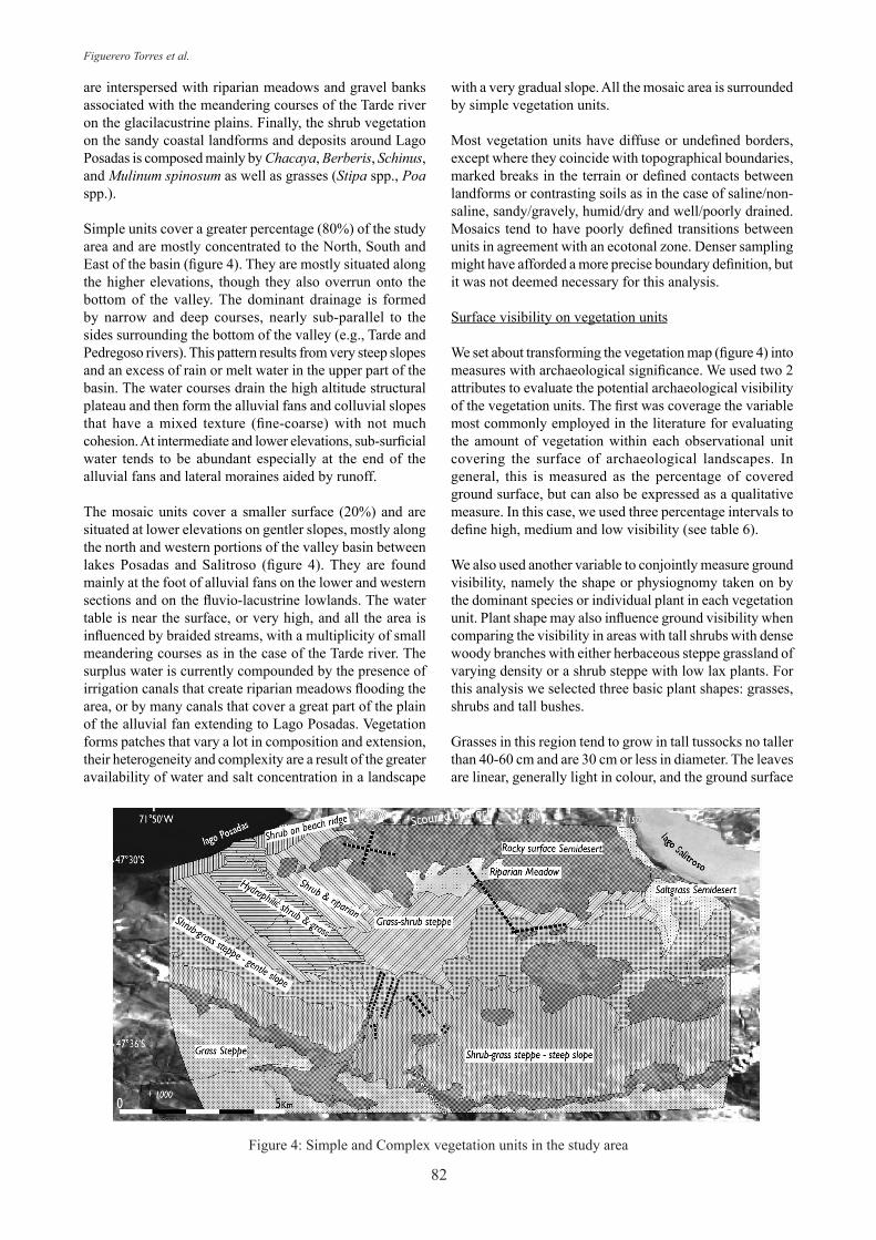
Simple units cover a greater percentage (80%) of the study area and are mostly concentrated to the North, South and East of the basin (figure 4). They are mostly situated along the higher elevations, though they also overrun onto the bottom of the valley. The dominant drainage is formed by narrow and deep courses, nearly sub-parallel to the sides surrounding the bottom of the valley (e.g., Tarde and Pedregoso rivers). This pattern results from very steep slopes and an excess of rain or melt water in the upper part of the basin. The water courses drain the high altitude structural plateau and then form the alluvial fans and colluvial slopes that have a mixed texture (fine-coarse) with not much cohesion. At intermediate and lower elevations, sub-surficial water tends to be abundant especially at the end of the alluvial fans and lateral moraines aided by runoff.

The mosaic units cover a smaller surface (20%) and are situated at lower elevations on gentler slopes, mostly along the north and western portions of the valley basin between lakes Posadas and Salitroso (figure 4). They are found mainly at the foot of alluvial fans on the lower and western sections and on the fluvio-lacustrine lowlands. The water table is near the surface, or very high, and all the area is influenced by braided streams, with a multiplicity of small meandering courses as in the case of the Tarde river. The surplus water is currently compounded by the presence of irrigation canals that create riparian meadows flooding the area, or by many canals that cover a great part of the plain of the alluvial fan extending to Lago Posadas. Vegetation forms patches that vary a lot in composition and extension, their heterogeneity and complexity are a result of the greater availability of water and salt concentration in a landscape

with a very gradual slope. All the mosaic area is surrounded by simple vegetation units.

Most vegetation units have diffuse or undefined borders, except where they coincide with topographical boundaries, marked breaks in the terrain or defined contacts between landforms or contrasting soils as in the case of saline/non-saline, sandy/gravely, humid/dry and well/poorly drained. Mosaics tend to have poorly defined transitions between units in agreement with an ecotonal zone. Denser sampling might have afforded a more precise boundary definition, but it was not deemed necessary for this analysis.

Surface visibility on vegetation units

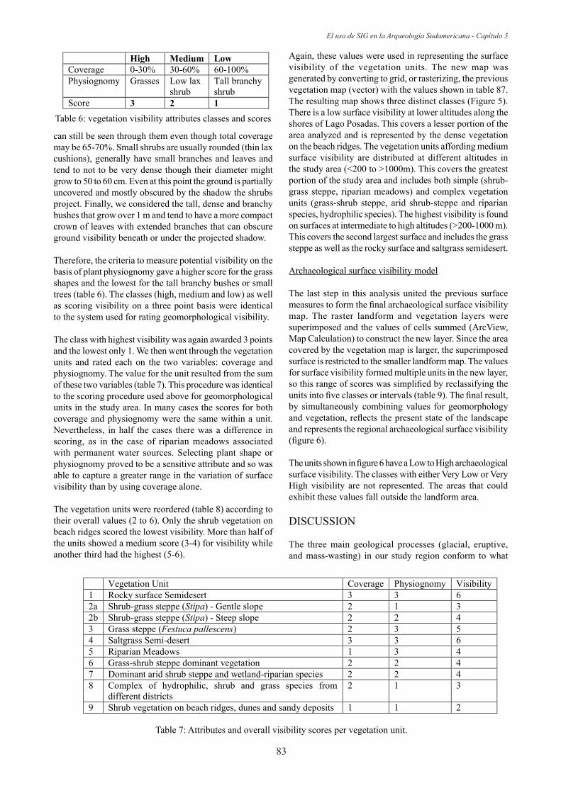
We set about transforming the vegetation map (figure 4) into measures with archaeological significance. We used two 2 attributes to evaluate the potential archaeological visibility of the vegetation units. The first was coverage the variable most commonly employed in the literature for evaluating the amount of vegetation within each observational unit covering the surface of archaeological landscapes. In general, this is measured as the percentage of covered ground surface, but can also be expressed as a qualitative measure. In this case, we used three percentage intervals to define high, medium and low visibility (see table 6).

We also used another variable to conjointly measure ground visibility, namely the shape or physiognomy taken on by the dominant species or individual plant in each vegetation unit. Plant shape may also influence ground visibility when comparing the visibility in areas with tall shrubs with dense woody branches with either herbaceous steppe grassland of varying density or a shrub steppe with low lax plants. For this analysis we selected three basic plant shapes: grasses, shrubs and tall bushes.

Grasses in this region tend to grow in tall tussocks no taller than 40-60 cm and are 30 cm or less in diameter. The leaves are linear, generally light in colour, and the ground surface

Figure 4: Simple and Complex vegetation units in the study area

83


can still be seen through them even though total coverage may be 65-70%. Small shrubs are usually rounded (thin lax cushions), generally have small branches and leaves and tend to not to be very dense though their diameter might grow to 50 to 60 cm. Even at this point the ground is partially uncovered and mostly obscured by the shadow the shrubs project. Finally, we considered the tall, dense and branchy bushes that grow over 1 m and tend to have a more compact crown of leaves with extended branches that can obscure ground visibility beneath or under the projected shadow.

Therefore, the criteria to measure potential visibility on the basis of plant physiognomy gave a higher score for the grass shapes and the lowest for the tall branchy bushes or small trees (table 6). The classes (high, medium and low) as well as scoring visibility on a three point basis were identical to the system used for rating geomorphological visibility.

The class with highest visibility was again awarded 3 points and the lowest only 1. We then went through the vegetation units and rated each on the two variables: coverage and physiognomy. The value for the unit resulted from the sum of these two variables (table 7). This procedure was identical to the scoring procedure used above for geomorphological units in the study area. In many cases the scores for both coverage and physiognomy were the same within a unit. Nevertheless, in half the cases there was a difference in scoring, as in the case of riparian meadows associated with permanent water sources. Selecting plant shape or physiognomy proved to be a sensitive attribute and so was able to capture a greater range in the variation of surface visibility than by using coverage alone.

The vegetation units were reordered (table 8) according to their overall values (2 to 6). Only the shrub vegetation on beach ridges scored the lowest visibility. More than half of the units showed a medium score (3-4) for visibility while another third had the highest (5-6).

Again, these values were used in representing the surface visibility of the vegetation units. The new map was generated by converting to grid, or rasterizing, the previous vegetation map (vector) with the values shown in table 87. The resulting map shows three distinct classes (Figure 5). There is a low surface visibility at lower altitudes along the shores of Lago Posadas. This covers a lesser portion of the area analyzed and is represented by the dense vegetation on the beach ridges. The vegetation units affording medium surface visibility are distributed at different altitudes in the study area (<200 to >1000m). This covers the greatest portion of the study area and includes both simple (shrub-grass steppe, riparian meadows) and complex vegetation units (grass-shrub steppe, arid shrub-steppe and riparian species, hydrophilic species). The highest visibility is found on surfaces at intermediate to high altitudes (>200-1000 m). This covers the second largest surface and includes the grass steppe as well as the rocky surface and saltgrass semidesert.

Archaeological surface visibility model

The last step in this analysis united the previous surface measures to form the final archaeological surface visibility map. The raster landform and vegetation layers were superimposed and the values of cells summed (ArcView, Map Calculation) to construct the new layer. Since the area covered by the vegetation map is larger, the superimposed surface is restricted to the smaller landform map. The values for surface visibility formed multiple units in the new layer, so this range of scores was simplified by reclassifying the units into five classes or intervals (table 9). The final result, by simultaneously combining values for geomorphology and vegetation, reflects the present state of the landscape and represents the regional archaeological surface visibility (figure 6).

The units shown in figure 6 have a Low to High archaeological surface visibility. The classes with either Very Low or Very High visibility are not represented. The areas that could exhibit these values fall outside the landform area.

DISCUSSION

The three main geological processes (glacial, eruptive, and mass-wasting) in our study region conform to what

High Medium Low Coverage 0-30% 30-60% 60-100% Physiognomy Grasses Low lax

shrub Tall branchy shrub

Score 3 2 1 Table 6: vegetation visibility attributes classes and scores

Vegetation Unit Coverage Physiognomy Visibility 1 Rocky surface Semidesert 3 3 6 2a Shrub-grass steppe (Stipa) - Gentle slope 2 1 3 2b Shrub-grass steppe (Stipa) - Steep slope 2 2 4 3 Grass steppe (Festuca pallescens) 2 3 5 4 Saltgrass Semi-desert 3 3 6 5 Riparian Meadows 1 3 4 6 Grass-shrub steppe dominant vegetation 2 2 4 7 Dominant arid shrub steppe and wetland-riparian species 2 2 4 8 Complex of hydrophilic, shrub and grass species from

different districts 2 1 3

9 Shrub vegetation on beach ridges, dunes and sandy deposits 1 1 2

Table 7: Attributes and overall visibility scores per vegetation unit.

84


is expected for the cordilleran region of Patagonia and their corresponding landforms are the minimum units in the landscape. The dominant feature of the climate is the year round water deficit compounded by the drying effect of the constant westerly winds and temperatures in this enclosed basin. This aridity has been more pronounced from AD 1960 onwards while at the same time there has been a sharp decrease in the intensive land use since the late 1980s. Therefore the variables we selected to evaluate the conditions that obscure or expose archaeological objects on the surface (texture, wind deflation, soil development, % organic matter Horizon A, fluvial deposits and mass wasting) were based on how the active processes on these landforms respond to the main factors of the local climate. In general, these coincide with many of the attributes employed when describing landforms in other areas of Patagonia (e.g. Ercollano et al 2000) though we additionally scored with a hierarchical quantitative measure.

Since our study area is a low lying basin located close to the NPI and the Andes mountains several biogeographical vegetation units (Western and Sub-Andean Districts and Sub-Antarctic Province) come into contact thus making it difficult to characterize the whole area for the purposes of our analysis. From these bigger divisions we focused on the smaller homogenous vegetation units that result from the active processes in the present day ecosystem climate. Again, water availability and temperature but also relief as well as the intensive land utilization for sheep farming

during the past 100 years are the most salient factors in shaping the minimum units identified on the basis of field censuses and aerial photographs. The attributes we selected and scored in this case were ground cover as well as plant physiognomy or shape.

One of our main concerns was in striving for a common scale of analysis in both local geology and vegetation. The scoring for visibility for landforms and vegetation was clearly established using hierarchical qualitative and quantitative values, allowing comparisons with other regions or surveys. What is relevant in this study is that the traditional measure for surface visibility (% ground cover) was established in regards to the vegetation unit. It therefore reflects the temporality of the processes shaping the unit and not the potentially short term or transitory conditions of a particular spot (e.g., 2-4 square meters) in the landscape. In this sense the measures used for vegetation and geomorphology share the same kind of temporality and are comparable in scale and resolution. This also means that vegetation was

Table 8: vegetation units ordered according to their relative ground visibility

Vegetation Visibility 9 Shrub vegetation on beach ridges, dunes and sandy deposits 2 2 a Shrub-grass steppe (Stipa) - Gentle slope 3 8 Complex of hydrophilic, shrub and grass species from different districts 3 2 b Shrub-grass steppe (Stipa) - Steep slope 4 5 Riparian Meadows 4 6 Grass-shrub steppe dominant vegetation 4 7 Dominant arid shrub steppe and wetland-riparian species 4 3 Grass steppe (Festuca pallescens) 5 4 Saltgrass Semi-desert 6 1 Rocky surface Semidesert 6

Figure 5: Ground visibility of the local vegetation

Scores Classes Visibility 7-9 1 Very Low 10-12 2 Low 13-15 3 Medium 16-18 4 High 19-21 5 Very High Table 9: regional archaeological surface visibility classes

85


rated independently and was not considered simply an attribute of a particular landform. Therefore, the shape and distribution of the units in the landform and vegetation maps are different. That is, they are not isomorphic because each responds differently to the environmental conditions though the water deficit and arid climate has a bearing in both cases.

The landform map covers the southern margin of the basin and has three main surface visibility scores (7-11) though the area with medium visibility (9-10) occupies a larger percentage of the mapped area. The areas with lower surface visibility correspond to moraines and are located towards the side of the valley at different heights (200-300 m, 400-500 m and 700-950 m). The vegetation map covers the entire valley floor and represents a bigger area than the geomorphic map. There is a broader range of surface values (2-6) since all are present in the area occupying the valley floor and sides, but the lowest surface visibility (2) is restricted to the beach ridges bordering the eastern end of Lago Posadas. Both maps then have greater portions with medium surface visibility values but the distribution of the areas is different. The combined values in the final map show a pattern of more continuous area with medium surface visibility mostly distributed on the bottom of the valley and other discontinuous areas with both lower and higher visibility situated on the valley sides.

This model then is a representation of the variations in the condition of the ground surface that is based exclusively on environmental features. The fact that it establishes the expected differences in ground visibility can be used in either of two ways. Firstly, to plan ahead the intensity and placement of observation units in pedestrian surveys for locating archaeological materials in order to ensure better coverage and choose the most appropriate survey techniques. Secondly, as a parameter for interpreting how representative are the archaeological materials in relation to what is potentially observable or for places already surveyed or in the literature. The coverage and resolution of the units used in constructing this model also make it suitable for approaches that contemplate continuous or discontinuously

distributed materials over the landscape. The way we have typified the degree of surface visibility could possibly be extended to the same landforms and vegetation in similarly located areas in Patagonia.

Archaeological materials in the Lago Posadas basin

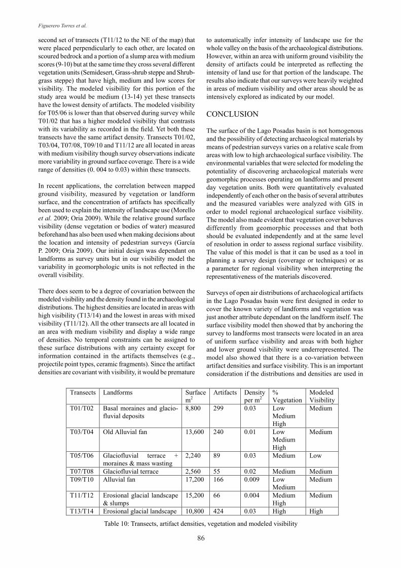
A survey of archaeological distributions in the Lago Posadas basin were carried out in the summer of 1999 while excavation of Cerro de los Indios 1 rockshelter was still underway. Transects were located in pairs on identified landforms in the valley and were 4 m wide though of varying length. All artifacts and ecofacts were continuously recorded within transects but at 200 m intervals (600 m on the longest transects) samples were collected (4x4m blocks) and more detailed observations made of the ground surface including vegetation cover. The list of transects together with artifact densities and vegetation are presented in the following table (table 10) and their location within the valley and associated landforms are indicated in figure 2.

Vegetation cover (%) was grouped into low, medium and high (see table 6) and table 10 lists all the classes observed in each pair of transects. What strikes us first is the variability of ground visibility within each landform as measured at the observation spots. However, using the frequency with which these classes occurred we would have described this area as somewhat uniform visibility, but without our being able to reach a regional assessment of the degree of this variability. Our concern at the time was focused on geomorphic processes which meant that vegetation cover was taken as descriptor of the corresponding landform and did not have an independent status or regional value. As a comparison in the last column of table 10 we have added the modeled visibility based on figure 6. Though four transects fall outside the visibility model, T13/14 in the NW of the area is located on scoured bedrock that is coincident with a vegetation unit (Semidesert) with a high visibility score. Therefore, this set of transects will have a high regional score, maybe even among the highest in the area we have surveyed and it also has the highest density of artifacts. The

Figure 6: Model of the regional archaeological surface visibility and the location of the archaeological survey transects

86


second set of transects (T11/12 to the NE of the map) that were placed perpendicularly to each other, are located on scoured bedrock and a portion of a slump area with medium scores (9-10) but at the same time they cross several different vegetation units (Semidesert, Grass-shrub steppe and Shrub-grass steppe) that have high, medium and low scores for visibility. The modeled visibility for this portion of the study area would be medium (13-14) yet these transects have the lowest density of artifacts. The modeled visibility for T05/06 is lower than that observed during survey while T01/02 that has a higher modeled visibility that contrasts with its variability as recorded in the field. Yet both these transects have the same artifact density. Transects T01/02, T03/04, T07/08, T09/10 and T11/12 are all located in areas with medium visibility though survey observations indicate more variability in ground surface coverage. There is a wide range of densities (0. 004 to 0.03) within these transects.

In recent applications, the correlation between mapped ground visibility, measured by vegetation or landform surface, and the concentration of artifacts has specifically been used to explain the intensity of landscape use (Morello et al. 2009; Oria 2009). While the relative ground surface visibility (dense vegetation or bodies of water) measured beforehand has also been used when making decisions about the location and intensity of pedestrian surveys (García P. 2009; Oria 2009). Our initial design was dependant on landforms as survey units but in our visibility model the variability in geomorphologic units is not reflected in the overall visibility.

There does seem to be a degree of covariation between the modeled visibility and the density found in the archaeological distributions. The highest densities are located in areas with high visibility (T13/14) and the lowest in areas with mixed visibility (T11/12). All the other transects are all located in an area with medium visibility and display a wide range of densities. No temporal constraints can be assigned to these surface distributions with any certainty except for information contained in the artifacts themselves (e.g., projectile point types, ceramic fragments). Since the artifact densities are covariant with visibility, it would be premature

to automatically infer intensity of landscape use for the whole valley on the basis of the archaeological distributions. However, within an area with uniform ground visibility the density of artifacts could be interpreted as reflecting the intensity of land use for that portion of the landscape. The results also indicate that our surveys were heavily weighted in areas of medium visibility and other areas should be as intensively explored as indicated by our model.

CONCLUSION

The surface of the Lago Posadas basin is not homogenous and the possibility of detecting archaeological materials by means of pedestrian surveys varies on a relative scale from areas with low to high archaeological surface visibility. The environmental variables that were selected for modeling the potentiality of discovering archaeological materials were geomorphic processes operating on landforms and present day vegetation units. Both were quantitatively evaluated independently of each other on the basis of several attributes and the measured variables were analyzed with GIS in order to model regional archaeological surface visibility. The model also made evident that vegetation cover behaves differently from geomorphic processes and that both should be evaluated independently and at the same level of resolution in order to assess regional surface visibility. The value of this model is that it can be used as a tool in planning a survey design (coverage or techniques) or as a parameter for regional visibility when interpreting the representativeness of the materials discovered.

Surveys of open air distributions of archaeological artifacts in the Lago Posadas basin were first designed in order to cover the known variety of landforms and vegetation was just another attribute dependant on the landform itself. The surface visibility model then showed that by anchoring the survey to landforms most transects were located in an area of uniform surface visibility and areas with both higher and lower ground visibility were underrepresented. The model also showed that there is a co-variation between artifact densities and surface visibility. This is an important consideration if the distributions and densities are used in

Transects Landforms Surface m2

Artifacts Density per m2

% Vegetation

Modeled Visibility

T01/T02 Basal moraines and glacio-fluvial deposits

8,800 299 0.03 Low Medium High

Medium

T03/T04 Old Alluvial fan 13,600 240 0.01 Low Medium High

Medium

T05/T06 Glaciofluvial terrace + moraines & mass wasting

2,240 89 0.03 Medium Low

T07/T08 Glaciofluvial terrace 2,560 55 0.02 Medium Medium T09/T10 Alluvial fan 17,200 166 0.009 Low

Medium Medium

T11/T12 Erosional glacial landscape & slumps

15,200 66 0.004 Medium High

Medium

T13/T14 Erosional glacial landscape 10,800 424 0.03 High High Table 10: Transects, artifact densities, vegetation and modeled visibility

87


inferring intensity of land use though a further step would be to precise the temporal constraints for these materials.

The consideration of temporal constraints and overall archaeological landscape distributions is relevant because of the noted increase in the amount of securely dated occupations in this region towards the end of the Holocene (Mengoni Goñalons et al. 2009) and the need to interpret its significance. Most of these occupations are in stratified sites (open air or rock shelters) but there are many open air scatters such as the distributions we have presented. The visibility model and the discussion we have put forward in this paper is a contribution on how to consider regional evidence without temporal constraints. The survey coverage and representativeness of archaeological distributions must be carefully examined before we can address the issues of persistence and intensity of occupations. Our proposal is that this starts with an evaluation of the overall surface visibility of the landscape under analysis. The design and construction of our surface visibility model can be used as a tool for either planning reconnaissance or in interpreting finds and allows more measured comparisons with results from other regions.

Acknowledgments

Field work for the archaeological (1999) and geomorphological (1998) surveys was financed with grants from the Universidad de Buenos Aires (UBACYT-TF97) and the Conicet (PIP 4628). Botanical field work, herbarium preparation and plant identification (2003-2004) as well as digitizing and SIG analysis was financed with grant UBACYT F617. Merrill Lyew, ESRI, and the late Eduardo Episcopo, Aeroterra, were instrumental in making the software accessible and in personally providing encouragement and support. The members of the Comisión de Fomento of Hipólito Yrigoyen gave us logistical support for setting up our camp headquarters. The local division of Gendarmeria Nacional, Sección Hipólito Yrigoyen, Escuadrón 39 Perito Moreno, generously lodged the whole team while the survey lasted. Alejandra Tejedo, Segemar, meticulously digitized the base maps. Norma Pérez-Reynoso designed and Ana Sánchez and Pamela Chávez collaborated in constructing the lab herbarium. Marcela Arrendondo, Carlos Aschero, María Páz Catá, Mariana De Nigris, Gabriela Ibañez, Alejandra Korstanje, Guillermo Mengoni Goñalons, Mariano Orcurto and Hugo Yacobaccio were part of the survey team during the 1999 field season, the company and friendship of them all is still much cherished.

REFERENCES

Aravena, J. C.2007 Reconstruction of climate variability from tree-ring records and glacier fluctuations in the southern Chilean Andes. Ph.D. University of Western Ontario, London-Ontario.

Aravena, J. C. and B. H. Luckman2009 Spatio-temporal rainfall patterns in Southern

South America. International Journal of Climatology 29 (14):2106-2120.

Aschero, C. A., M. T. Civalero, D. Bozzuto, M. De Nigris, A. Di Vruno, V. Dolce, N. Fernández, L. González and P. Limbruner2009 El registro arqueológico de la costa norte del lago Pueyrredón-Cochrane. In Arqueología de Patagonia: una mirada desde el último confín, edited by M. Salemme, F. Santiago, M. Álvarez, E. Piana, M. Vázquez and M. E. Mansur, pp. 919-926. vol. II. 2 vols. Editorial Utopías, Ushuaia.

Aschero, C. A., M. E. De Nigris, M. J. Figuerero Torres, A. G. Guráieb, G. L. Mengoni Goñalons and H. D. Yacobaccio1999 Excavaciones recientes en Cerro de los Indios 1, Lago Posadas (Santa Cruz): nuevas perspectivas. In. Soplando en el viento ... Actas de las Terceras Jornadas de Arqueología de la Patagonia, pp. 269-286. Universidad del Comahue, Neuquén.

Attenbrow, V.2006 What’s changing: population size or land-use patterns? The archaeology of Upper Mangrove Creek, Sydney Basin. Terra Australis 21:1-380.

Banning, E. B.2002 Archaeological Survey. Kluwer Academic / Plenum Publishers, New York.

Barbería, E. M.1996 Los dueños de la tierra en la patagonia austral 1880-1920. UNPA, Río Gallegos.

Barton, C. M., J. Bernabeu, J. E. Aura, O. Garcia and N. La Roca2002 Dynamic landscapes, artifact taphonomy, and landuse modeling in the western Mediterranean. Geoarchaeology 17 (2):155-190.

Barton, C. M., J. Bernabeu, J. E. Aura, O. Garcia, S. Schmich and L. Molina2004 Long-Term Socioecology and Contingent Landscapes. Journal of Archaeological Method and Theory 11 (3):253-295.

Bevan, A. and J. Conolly2004 GIS, Archaeological Survey, and Landscape Archaeology on the Island of Kythera, Greece. Journal of Field Archaeology 29 (1/2):123-138.

Bintliff, J.1999 The Hidden Landscape of Prehistoric Greece. Journal of Mediterranean Archaeology 12 (2):139-168.

Bintliff, J., M. Kuna and N. Venclova (editors)2000 The Future of Surface Artefact Survey in Europe. Sheffield Academic Press, Sheffield.

Brunswig de Bamberg, M.1995 Allá en la patagonia. la vida de una mujer en una

88


tierra inhóspita. Vergara, Buenos Aires.

Burger, O., L. C. Todd, P. Burnett, T. J. Stohlgren and D. Stephens2004 Multi-Scale and nested-intensity sampling techniques for archaeological survey. Journal of Field Archaeology 29 (3/4):409-423.

Campana, S. and R. Francovich2007 Understanding Archaeological Landscapes: Steps Towards an Improved Integration of Survey Methods in the Reconstruction of Subsurface Sites in South Tuscany. In Remote Sensing in Archaeology, edited by J. Wiseman and F. El-Baz, pp. 239-261. Interdisciplinary Contributions To Archaeology. Springer, New York.

Cashmere, C. and L. Wandsnider1997 GIS modelling of Archaeological Surface Visibility at Agate Fossil Beds. In Agate Fossil Beds Prehistoric Archaeological landscapes, 1994-1995. Report on 1994 and 1995 Archaeological activities by the department of Anthropology, University of Nebraska-Lincoln and the NPS Midwest Archaeological Center at Agate Fossil Beds National Monument, edited by L. Wandsnider and G. H. MacDonell, pp. 13-25. Midwest Archaeological Center, National Park Service, Lincoln.

Cassiodoro, G., A. G. Guráieb, A. Re and A. Tívoli 2004 Distribución de recursos líticos en el registro superficial de la cuenca de los lagos Pueyrredón-Posadas-Salitroso. In Contra viento y marea, edited by T. Civalero, P. Fernández and A. G. Guráieb, pp. 57-70. INAPL, Buenos Aires.

Cibils, A. F. and P. R. Borrelli2005 Grasslands of Patagonia. In Grasslands of the World, edited by J. M. Suttie, S. G. Reynolds and C. Batello, pp. 121-170. Plant Production and Protection Series No. 34. FAO, Rome.

Cosgrove, R.1999 Forty-Two Degrees South: The Archaeology of Late Pleistocene Tasmania. Journal of World Prehistory 13 (4):357-402.

De Nigris, M. E. and M. P. Catá2005 Cambios en los patrones de representación ósea del guanaco en Cerro de los Indios 1 (Lago Posadas, Santa Cruz). Intersecciones en Antropología 6:109-119.

De Nigris, M. E., M. J. Figuerero Torres, A. G. Guráieb and G. L. Mengoni Goñalons2004 Nuevos fechados radiocarbónicos de la localidad de Cerro de los Indios 1 (Santa Cruz) y su proyección areal. In Contra viento y marea. Arqueología de Patagonia, edited by T. Civalero, P. Fernández and A. G. Guráieb, pp. 537-544. INAPL, Buenos Aires.

del Valle, H. F.2003 Degradación de la tierra en la patagonia extrandina: Estrategias de la percepción remota. In Desertificación. Indicadores y puntos de referencia en America Latina

y El Caribe, edited by E. Abraham, D. Tomasini and P. Maccagno, pp. 131-144. Zeta Editores, Mendoza.

Ercolano, B., F. Carballo Marina and E. Mazzoni2000 El uso del espacio por parte de poblaciones cazadoras-recolectoras en la cuenca inferior del río Gallegos, extremo sur de Patagonia, Argentina. Anales del Instituto de la Patagonia (Serie Ciencias Sociales) 28:233-250.

Fanning, P. C. and S. J. Holdaway2002 Using geospatial technologies to understand prehistoric human/landscape interaction in arid Australia. Arid Lands Newsletter 51 (May/June).

Figuerero Torres, M. J.2004 La estructuración del espacio a través del tiempo en Cerro de los Indios 1 (Lago Posadas, Santa Cruz). In Contra viento y marea. Arqueología de Patagonia, edited by T. Civalero, P. Fernández and A. G. Guráieb, pp. 557-563. INAPL, Buenos Aires.

García P., C.2009 Cazadores recolectores en el área lacustre de la vertiente occidental andina (39°S): cronología, contextos y procesos. In Arqueología de Patagonia: una mirada desde el último confín, edited by M. Salemme, F. Santiago, M. Álvarez, E. Piana, M. Vázquez and M. E. Mansur, pp. 1011-1022. vol. II. Editorial Utopías, Ushuaia.

Gilli, A., D. Ariztegui, F. S. Anselmetti, J. A. McKenzie, V. Markgraf, I. Hajdas and R. D. McCulloch2005 Mid-Holocene strengthening of the Southern Westerlies in South America — sedimentological evidences from Lago Cardiel, Argentina (49°S). Global and Planetary Change Historical and Holocene glacier - climate variations 49:75–93.

Glasser, N. F., S. Harrison, V. Winchester and M. Aniya2004 Late Pleistocene and Holocene palaeoclimate and glacier fluctuations in Patagonia. Global and Planetary Change 43:79-101.

Glasser, N. F. and K. Jansson2005 Fast-flowing outlet glaciers of the Last Glacial Maximum Patagonian Icefield. Quaternary Research 63:206-211.

Goñi, R. A., G. Barrientos and G. Cassiodoro2000-2002 Condiciones previas a la extinción de las poblaciones humanas del sur de Patagonia: una discusión a partir del análisis del registro arqueológico de la cuenca del lago Salitroso. Cuadernos del Instituto Nacional de Antropología y Pensamiento Latinoamericano 19:249-266.

Guráieb, A. G.2004 Before and after the hiatus: lithic technology in Cerro de los Indios 1 rockshelter, south Patagonia, Argentina. Before Farming 2004/3 (1):1-19.

Hein, A. S., N. R. J. Hulton, T. J. Dunai, D. E. Sugden, M. R. Kaplan and S. Xu

89


2010 The chronology of the Last Glacial Maximum and deglacial events in central Argentine Patagonia. Quaternary Science Reviews 29 (9-10):1212-1227.

Holdaway, S. J., P. C. Fanning and J. Shiner2006 Geoarchaeological investigation of aboriginal landscape occupation in Paroo-Darling National Park, Western NSW, Australia. Research in Anthropology & Linguistics-E 1:1-82.

Holdaway, S. J. and L. Wandsnider2006 Temporal Scales and Archaeological landscapes from Eastern Desert of Australia and Intermontane North America. In Confronting Scale in Archaeology. Issues of Theory and Practice, edited by G. Lock and B. L. Molyneaux, pp. 183-202. Springer, New York.

Honeychurch, W., J. Wright and C. Amartuvshin2007 A nested approach to survey in the Egiin Gol Valley, Mongolia. Journal of Field Archaeology 32:339-352.

Hubbard, A., A. S. Hein, M. R. Kaplan, N. R. J. Hulton and N. Glasser2005 A modelling reconstruction of the last glacial maximum ice sheet and its deglaciation in the vicinity of the Northern Patagonian Icefield, South America. Geografiska Annaler, Series A: Physical Geography 87 (2):375-391.

Ivanoff Wellman, D.2002 La Guerra de Chile Chico o los sucesos del Lago Buenos Aires. 3 ra. ed. Ediciones Cruz del Sur de la Trapananda, Valparaíso.

León, R. J. C., D. Bran, M. Collantes, J. M. Paruelo and A. Soriano1998 Grandes unidades de vegetación de la patagonia extra andina. Ecología Austral 8:125-144.

Lock, G. and B. L. Molyneaux2006 Introduction: Confronting scale. In Confronting Scale in Archaeology. Issues of Theory and Practice, edited by G. Lock and B. L. Molyneaux, pp. 1-11. Springer, New York.

Masiokas, M. H., R. Villalba, B. H. Luckman, M. E. Lascano, S. Delgado and P. Stepanek2008 20th-century glacier recession and regional hydroclimatic changes in northwestern Patagonia. Global and Planetary Change Historical and Holocene glacier - climate variations 60 (1-2):85-100.

Mena L., F. and D. Jackson S.1991 Tecnología y subsistencia en Alero Entrada Baker Región de Aisen, Chile. Anales del Instituto de la Patagonia (Serie Ciencias Sociales) 20:169-203.

Méndez, C. and H. Velázquez2005 Tecnología y subsistencia en Alero Entrada Baker: una revisión a la luz de nuevos antecedentes. In Actas del XVI Congreso Nacional de Arqueología Chilena, pp. 593-602. Ediciones Escaparate, Concepción.

Mengoni Goñalons, G. L.1999 Cazadores de guanacos de la estepa patagónica. Colección Tesis Doctorales. Sociedad Argentina de Antropología, Buenos Aires.

Mengoni Goñalons, G. L., M. J. Figuerero Torres, P. V. Chávez and M. V. Fernández2009 Cronología de las ocupaciones arqueológicas del área Los Antiguos-Monte Zeballos y Paso Roballos (N.O. de Santa Cruz). In Tras la senda de los ancestros: arqueología de Patagonia, edited by P. F. Azar, E. M. Cúneo and S. N. Rodríguez de Torcigliani, pp. 1-11. EDUCO, Neuquén.

Mengoni Goñalons, G. L. and H. D. Yacobaccio2000 Arqueología de Cerro de los Indios y su entorno. Arqueología 10:193-201.

Morello, F., L. A. Borrero, J. Torres, M. Massone, M. Arroyo, R. McCulloch, E. Calas, M. Lucero, I. Martínez and G. Bahamonde2009 Evaluando el registro arqueológico de Tierra del Fuego durante el Holoceno temprano y medio. In Arqueología de Patagonia: una mirada desde el último confín, edited by M. Salemme, F. Santiago, M. Álvarez, E. Piana, M. Vázquez and M. E. Mansur, pp. 1075-1091. vol. II. Editorial Utopías, Ushuaia.

Moy, C. M., R. B. Dunbar, P. I. Moreno, J.-P. Francois, R. Villa-Martínez, D. M. Mucciarone, T. P. Guilderson and R. D. Garreaud2008 Isotopic evidence for hydrologic change related to the westerlies in SW Patagonia, Chile, during the last millennium. Quaternary Science Reviews 27 (13-14):1335-1349.

Oliva, G.2006 Perspectivas de control de la desertificación en la Patagonia luego de 15 años de esfuerzos. In Taller Grupo de Estudio Pastizales Patagonicos - FAO. Degradacion de Ecosistemas Pastoriles en la Patagonia. Serie Actas, edited by C. Hepp K., pp. 11-20. Instituto de Investigaciones Agropecuarias. Serie Actas 36, Coyhaique.

Oria, J.2009 Prospecciones en el interior de la estepa fueguina. In Arqueología de Patagonia: una mirada desde el último confín, edited by M. Salemme, F. Santiago, M. Álvarez, E. Piana, M. Vázquez and M. E. Mansur, pp. 1109-1125. Editorial Utopías, Ushuaia.

Rabassa, J.2008 Late Cenozoic Glaciations in Patagonia and Tierra del Fuego. In The Late Cenozoic of Patagonia and Tierra del Fuego, edited by J. Rabassa, pp. 151-204. Developments in Quaternary Sciences. vol. 11. Elsevier, Amsterdam-Boston-Oxford.

Ramenofsky, A. F. and A. Steffen1998 Units as Tools of Measurements. In Unit Issues in Archaeology: measuring time, space and material, edited by A. F. Ramenofsky and A. Steffen, pp. 3-17. University

90


of Utah Press, Salt Lake City.

Ramos, V.2002a El Magmatismo Neógeno de la Cordillera Patagónica. In Geología y Recursos Naturales de Santa Cruz, edited by M. J. Haller, pp. 1-13. vol. Relatorio I-12. XV Congreso Geológico Argentino, El Calafate.

2002b El Magmatismo Paleógeno de la Cordillera Patagónica. In Geología y Recursos Naturales de Santa Cruz, edited by M. J. Haller, pp. 1-10. vol. Relatorio I-10. XV Congreso Geológico Argentino, El Calafate.

Rhodes, E. J., P. C. Fanning, S. J. Holdaway and C. Bolton2009 Archaeological surfaces in western NSW: Stratigraphic contexts and preliminary OSL dating of hearths. In Archaeological Science Under a Microscope. Studies in Residue and Ancient DNA Analysis in Honour of Thomas H. Loy, edited by M. Haslam, G. Robertson, A. Crowther, S. Nugent and L. Kirkwood. Terra Australis 30:189-200.

Salemme, M., F. Santiago, M. Álvarez, E. Piana, M. Vázquez and M. E. Mansur2009 Arqueología de Patagonia: una mirada desde el último confín. Editorial Utopías, Ushuaia.

Santa Cruz:AER Los Antiguos2009 Reportes anuales. Agrometeorología http://www.inta.gov.ar/santacruz/met/reportes.htm (21 de Agosto, 2009).

Schiffer, M. B., A. P. Sullivan and T. C. Klinger1978 The design of archaeological surveys. World Archaeology 10 (1):1-28.

Singer, B. S., R. P. Ackert and H. Guillou2004 40Ar/39Ar and K-Ar chronology of Pleistocene glaciations in Patagonia. GSA Bulletin 116 (3/4):434-450.

Soriano, A.1956 La vegetación de la República Argentina. IV. Los distritos florísticos de la Provincia Patagónica. Revista de Investigaciones Agrícolas 10 (4):323-347.

1958 Los distritos florísticos de la Provincia Patagónica. Revista de Investigaciones Agrícolas 10 (4):323-347.

Spennemann, D. H. R.1995 Site visibility and site survey bias in cultural resource management. A preliminary analysis of the 1993 survey reports held by Aboriginal Affairs Victoria. Report Nº 19. The Johnstone Centre of Parks, Recreation and Heritage, Charles Sturt University, Albury.

Terrenato, N. and A. J. Ammerman1996 Visibility and Site Recovery in the Cecina Valley Survey, Italy. Journal of Field Archaeology 23 (1):91-109.

Thompson, S.2004 Side-by-Side and Back-to-Front: Exploring Intra-Regional Latitudinal and Longitudinal Comparability in

Survey Data. Three Case Studies from Metaponto, Southern Italy. In Side-By-Side Survey: Comparative Regional Studies in the Mediterranean World, edited by J. Cherry and S. E. Alcock, pp. 65-85. Oxbow Books, Oxford.

Torrence, R., J. Specht and B. Boyd1999 Archaeological Fieldwork on Numundo and Garu Plantations West New Britain, PNG. PNG National Museum and Art Gallery, Australia and Pacific Foundation, West New Britain Palm Oil, Ltd.

van Leusen, P. M.2002 Pattern to process: methodological investigations into the formation and interpretation of spatial patterns in archaeological landscapes. Ph.D. dissertation, Rijksuniversiteit Groningen, Groningen.

Villalba, R., A. Lara, J. Boninsegna, M. Masiokas, S. Delgado, J. C. Aravena, F. A. Roig, A. Schmelter, A. Wolodarsky and A. Ripalta2003 Large-Scale Temperature Changes across the Southern Andes: 20th-Century Variations in the Context of the Past 400 Years. Climatic Change 59 (1-2):177-232.

Wagner, S., M. Widmann, J. Jones, T. Haberzettl, A. Lucke, C. Mayr, C. Ohlendorf, F. Schabitz and B. Zolitschka2007 Transient simulations, empirical reconstructions and forcing mechanisms for the Mid-holocene hydrological climate in southern Patagonia. Climate Dynamics 29 (4):333-355

Wandsnider, L. and E. Camilli1996 The character of surface deposits and its influence on survey adequacy. Journal of Field Archaeology 19 (2):169-188.

Wandsnider, L. and M. A. Dooley2004 Landscape Approaches to Regional Archaeological Variation. Electronic Symposium: Survey Methodologies in Global Archaeological Contexts. Paper presented at the 69th Annual Meeting of the Society for American Archaeology, Montreal.

Wheatly, D. and M. Gillings2000 Vision, perception and GIS. In Beyond the map: archaeology and spatial technologies, edited by G. Lock, pp. 123-131. Archaeopress, Oxford.

Witter, D. C.2004 Regional variation of the archaeology in Western New South Wales. Rangelands Journal 26 (2):129-149.

Zolitschka, B., F. Schabitz, A. Lucke, H. Corbella, B. Ercolano, M. Fey, T. Haberzettl, S. Janssen, N. Maidana, C. Mayr, C. Ohlendorf, G. Oliva, M. M. Páez, G. H. Schleser, J. Soto, P. Tiberi and M. Wille2006 Crater lakes of the Pali Aike Volcanic Field as key sites for paleoclimatic and paleoecological reconstructions in southern Patagonia, Argentina. Journal of South American Earth Sciences 21:294–309.

Date post:	01-Jan-2017
Category:	Documents
Upload:	trinhbao
View:	215 times
Download:	0 times

El uso de Sistemas de Información Geográfica (SIG) en arqueología ...

Documents