16

Experimental Prediction of Heat Transfer Correlations in Heat Exchangers

Tomasz Sobota Cracow University of Technology

Poland

1. Introduction

Heat exchangers is a broad term related to devices designed for exchanging heat between

two or more fluids with different temperatures. In most cases, the fluids are separated by a

heat-transfer surface. Heat exchangers can be classified in a number of ways, depending on

their construction or on how the fluids move relative to each other through the device. The

use of heat exchangers covers the following areas: the air conditioning, process, power,

petroleum, transportation, refrigeration, cryogenic, heat recovery, and other industries

applications. Common examples of heat exchangers in everyday use are air preheaters and

conditioners, automobile radiators, condensers, evaporators, and coolers. (Kuppan, 2000).

Many factors enter into the design of heat exchangers, including thermal analysis, size,

weight, structural strength, pressure drop, and cost. Cost evaluation is obviously an

optimization process dependent upon the other design parameters (Pitts & Sissom, 1998).

Economics plays a key role in the design and selection of heat exchanger equipment, and the

engineer should bear this in mind when taking up any new heat transfer design problem.

The weight and size of heat exchangers are significant parameters in the overall application

and thus may still be considered as economic variables (Holman, 2009; Shokouhmand et al.,

2008; Rennie & Raghavan, 2006).

Calculations of heat exchangers can be divided into two categories, namely, thermo-

hydraulic and mechanical design calculations. The subject of thermal and hydraulic

calculations is to determine heat-transfer rates, heat transfer area and pressure drops needed

for equipment sizing. Mechanical design calculations are concerned with detailed

equipment specifications, including stress analyses.

Heat exchanger problems may also be considering as rating or design problems. In a rating

problem, should be determined whether particular exchanger will perform a given heat-

transfer duty adequately. It is of no importance whether the exchanger physically exists or

whether it is specified only on paper. In a design problem, one must determine the

specifications for a heat exchanger that will handle a given heat-transfer duty. A rating

problem also arises when it is desired to use an existing heat exchanger in a new or

modified application (Serth, 2007). A particular application will dictate the rules that one

must follow to obtain the best design commensurate with economic considerations, size,

weight, etc. They all must bee considered in practice (Holman, 2009; Shokouhmand et al.,

2008; Rennie & Raghavan, 2006).

www.intechopen.com

Developments in Heat Transfer

294

2. Thermal design of the heat exchangers

The suitable use of heat transfer knowledge in the design of practical heat transfer equipment

is an art. Designers must be constantly aware of the differences between the idealized

conditions under which the fundamental knowledge was obtained and the real conditions of

their design and its environment. The result must satisfy process and operational requirements

and do so cost-effectively. An important element of any design process is to consider and

compensate the consequences of error in the basic knowledge, in its subsequent incorporation

into a design method. Heat exchanger design is not a extremely accurate procedure under

the best of conditions (Shilling et al., 1999).

The design of a heat exchanger usually consists the subsequent steps:

1. Specification of the process conditions, e.g. flow compositions, flow rates, temperatures,

pressures.

2. Obtaining of the required physical properties over the temperature and pressure ranges

of interest obtained.

3. Choosing the type of heat exchanger that is going to be used.

4. An initial estimation of the size of the heat exchanger that is made, using a heat transfer

coefficient appropriate to the fluids, the process, and the equipment.

5. A first design is chosen, complete in all details necessary to carry out the design

calculations.

6. Evaluation of ability to perform the process specifications with respect to both heat

transfer and pressure drop as the design of heat exchanger is chosen.

7. Described in point above procedure can be repeated to new heat exchanger design if it

is necessary. The final design should meet process requirements within reasonable error

expectations.

The calculation of convective heat transfer coefficients constitutes a crucial issue in

designing and sizing any type of heat exchange device. Thus its correct determining permits

for the proper selection of heat transfer area during designing of heat exchangers and

calculation of the fluids outlet temperature. A lot efforts have been made during

experimental investigations of pressure drop and heat transfer in different types of heat

exchangers to obtain proper heat transfer correlation formulas.

2.1 The Wilson plot technique to determine heat transfer correlations in heat exchangers

One of the widely used methods for calculations of heat transfer coefficient is the Wilson

plot technique. This approach was developed by E.E. Wilson in 1915 in order to evaluate the

heat transfer coefficients in shell and tube condensers for the case of a vapour condensing

outside by means of a cooling liquid flow inside (Viegas et al., 1998; Kumar et al., 2001; Rose,

2004; Fernández-Seara et al., 2007). It is based on the separation of the overall thermal

resistance into the inside convective thermal resistance and the remaining thermal

resistances participating in the heat transfer process. The overall thermal resistance Roveral of

the condensation process in a shell-and-tubes heat exchanger can be expressed as the sum of

three constituent thermal resistances: Rin – the internal convection, Rwall – the tube wall and

Ro – the external convection, presented in Eq. (1).

total in wall oR R R R= + + . (1)

www.intechopen.com

Experimental Prediction of Heat Transfer Correlations in Heat Exchangers

295

The thermal resistances of the fouling in Eq. (1) was neglected. Employing the expressions for the thermal resistances in Eq. (1), the overall thermal resistance can be rewritten as follows:

ln1 1

2

o

intotal

in in wall wall o o

d

dR

h A L h Aπλ⎛ ⎞⎜ ⎟⎝ ⎠= + + . (2)

where hin and ho is the internal and outer heat transfer coefficients, din and do – the inner and

outer tube diameters, λwall is the tube material thermal conductivity, Lwall is the tube length and Ai and Ao are the inner and outer tube surface areas, respectively. On the other hand, the overall thermal resistance can be written as a function of the overall heat transfer coefficient referred to the inner or outer tube surfaces and the corresponding areas. Assuming this the overall thermal resistance is expressed as a function of the overall heat transfer coefficient referred to the inner or outer surface Uin/o and the inner or outer surface area Ain/o (Eq. 3)

1

totalin o in o

RU A

= . (3)

Taking into account the specific conditions of a shell and tube condenser Wilson assumed that if the mass flow of the cooling liquid was modified, then the change in the overall thermal resistance would be mainly due to the variation of the in-tube heat transfer coefficient, while the remaining thermal resistances remained nearly constant. Therefore, as specified in Eq. (4) the thermal resistances outside of the tubes and the tube wall could be regarded as constant:

1wall oR R C+ = . (4)

Wilson determined that for the case of fully developed turbulent flow inside a tube of circular cross-section, the heat transfer coefficient was proportional to a power of the reduced velocity wr which describes the variations of the fluid property and the tube diameter. Thus, the heat transfer coefficient could be written in form:

2n

in rh C w= , (5)

where C2 is a constant, wr – the reduced fluid velocity and n – velocity exponent. In this case the convective thermal resistance related to the inner tube flow is proportional to 1 n

rw . Inserting Eqs. (4) and (5) into Eq. (1), the overall thermal resistance becomes the linear function of 1 n

rw , where C1 is the intercept and ( )21 inC A is the slope of the straight line. The overall thermal resistance can be calculated using experimental data using the following formula:

o o lmQ U A T= Δ . (6)

Substituting Eq. (3) into Eq. (6), and assuming ( )1 1 1 1p outlet inletQ m c T T= −$ , where 1m$ is the mass flow rate of cooling liquid, cp1 – average specific heat of cooling liquid, and T1inlet, T1outlet, are inlet and outlet temperatures of cooling liquid, respectively, yields to

www.intechopen.com

Developments in Heat Transfer

296

( )1 1 1 1

lmtotal

p outlet inlet

TR

m c T T

Δ= −$. (7)

As the constants C1 and C2 are determined from straight–line approximation of measured data, to evaluation, for a given mass flow rate, the internal heat transfer coefficient can be used Eq. (5) and internal heat transfer coefficient Eq. (8):

( )1

1o

o wall

hA C R

= − . (8)

The original Wilson plot technique depends on the knowledge of the overall thermal resistance, that involves to remain of one fluid flow rate constant and varying flow rate of the another fluid. Approach of Wilson plot technique to determine constant in heat transfer correlation formula for helically coiled tube-in-tube heat exchanger is presented by Sobota (Sobota, 2011).

3. Experimental prediction of heat transfer correlations in heat exchangers

In this chapter, the experimental and numerical investigations of helically coiled tube-in-tube heat exchanger are presented. Calculations of unknown constants and exponents in correlations formula for Nusselt number have been performed with least squares method using Levenberg-Marquardt algorithm. Presented method allows for determining unknown values of constants and exponents in correlation formulas for Nusselt number. This method enables to obtain values of heat transfer coefficient on both sides of the barrier simultaneously without earlier indirect calculations of the overall heat transfer.

3.1 Mathematical formulation of the inverse problem The issue consisting of simultaneous determining of the heat transfer coefficient on the cooling and heating liquid is ranked among inverse heat transfer problems (IHCP) (Beck et al., 1985). In discussed methodology the knowledge of correlation formula form for heat transfer coefficient on the both sides of the heat transfer surface, for counter-flow and parallel-flow heat exchanger, was assumed to be known. An unknown value of the parameters in correlation formulas was hidden in equations for outlet temperature of the liquids (Nashchokin, 1980):

a) parallel-flow arrangement of heat exchanger

- heating liquid

( )1

2 1

1

1, 1, 1, 2,1

2

1 e

1

ck FW

W W

calc meas meas measT T T TW

W

⎛ ⎞ ⋅− + ⋅⎜ ⎟⎝ ⎠−′′ ′ ′ ′= − −+

(9)

- cooling liquid

( )1

2 1

1

12, 2, 1, 2,

12

2

1 e

1

ck FW

W W

calc meas meas meas

WT T T T

WWW

⎛ ⎞ ⋅− + ⋅⎜ ⎟⎝ ⎠−′′ ′ ′ ′= + − + (10)

www.intechopen.com

Experimental Prediction of Heat Transfer Correlations in Heat Exchangers

297

b) counterflow arrangement of heat exchanger

- heating liquid

( )1

2 1

1

2 1

1

1, 1, 1, 2 ,1

1

2

1 e

1 e

c

c

k FW

W W

calc meas meas meas k FW

W W

T T T T

W

W

⎛ ⎞ ⋅− − ⋅⎜ ⎟⎝ ⎠⎛ ⎞ ⋅− − ⋅⎜ ⎟⎝ ⎠

−′′ ′ ′ ′= − −−

(11)

- cooling liquid

( )1

2 1

1

2 1

1

12, 2, 1, 2,

121

2

1 e

1 e

c

c

k FW

W W

calc meas meas meas k FW

W W

WT T T T

WW

W

⎛ ⎞ ⋅− − ⋅⎜ ⎟⎝ ⎠⎛ ⎞ ⋅− − ⋅⎜ ⎟⎝ ⎠

−′′ ′ ′ ′= + −−

(12)

where 1,measT′ and 2,measT′ – measured temperature of the heating and cooling liquid at the

inlet of the helically coiled heat exchanger respectively, °C; 1,calcT′′ and 2,calcT′′ – calculated

temperature of the heating and cooling liquid at the outlet of the helically coiled heat

exchanger respectively, °C; and expression W = V⋅ρ⋅cv is called as water equivalent. The minimum of the square of the differences between measured and calculated from analytical formula temperatures of the hot fluid and differences between measured and calculated from analytical formula temperatures of the cold fluid at the outlet of heat exchanger was searching for:

( ) ( ) ( )2 2

1, 1, 2 , 2 ,1

minn

meas calc meas calci

S T T T T=⎡ ⎤′′ ′′ ′′ ′′= − + − →⎢ ⎥⎣ ⎦∑α . (13)

In analysed example the solution of the nonlinear least square problem was searching for. Determining the values of the constants, and indirectly the values of heat transfer coefficient, was carried out using least squares method with modified Levenberg-Marquardt algorithm (Visual Numerics, 2007; Press et al., 1996). In Levenberg-Marquardt algorithm unknown are formed an column vector x = (x1, x2, ..., xm)T, for which the sum becomes minimum

( ) ( ) 2

1

minn

ii

S r=

= ⎡ ⎤ →⎣ ⎦∑x x , (14)

where ( )i meas calcr T T′′ ′′= −x . The method performs the k-th iteration as

( ) ( ) ( )1k k k+ = +x x δ , (15)

where

( ) ( )( ) ( ) ( ) ( )( ) ( )1

, 0, 1, ...T T

k k k k km m n m kμ −⎡ ⎤= + ⎡ − ⎤ =⎢ ⎥ ⎣ ⎦⎣ ⎦δ J J I J f T x . (16)

www.intechopen.com

Developments in Heat Transfer

298

The symbols f and Tm(x) stand for vector of measured and vector of computed temperature, respectively. Jacobian determinant is described by formula

( ) ( )m i

m Tj

mxn

r

x

⎡ ⎤⎛ ⎞∂ ∂⎢ ⎥⎜ ⎟= = ⎜ ⎟∂∂ ⎢ ⎥⎝ ⎠⎣ ⎦r x x

Jx

, (17)

where i = 1, …, n, j = 1, …, m, D(k) denotes diagonal matrix with positive elements. Quite often D(k) = Im, where Im is identity matrix.

The value of the parameter μ(k) → 0 when x(k) → x*. In the proximity of minimum x* the iteration step in the Levenberg-Marquardt method is almost the same as in the Gauss-Newton method. The computation programs for solving the non-linear least square problem by the Levenberg-Marquardt method are described in (Lawson & Hanson, 1974) and in the IMSL Library (Visual Numerics, 2007).

3.2 Correlations for Nusselt number

Although curved pipes are used in a wide range of applications, flow in curved pipes is relatively less well known than that in straight ducts. A helical coil can be geometrically

described by the coil radius R, the pipe radius r, and the coil pitch 2πb (Fig. 1).

Fig. 1. Schematic representation of a helical pipe with its main geometrical parameters:

r – tube radius; R – coil radius; 2πb – coil pitch

The observations on the complexity of a flow in such a channels allowed to notice the effect of curvature on the fluid flow regime which occurs delaying the transition from laminar to transitional flow to a higher Reynolds number with respect to straight pipes (Ito, 1959; Schmidt, 1967). Using data from his own experiments as well as that from previous investigations, Ito developed the following empirical relation to determine the critical Reynolds number for the range of curvature ratios of 1/15 to 1/860:

( )0.32Re 20000crit

rR

= , (18)

whilst Schmidt suggested the form of critical Reynolds number listed below:

0.45

Re 2300 1 8.6crit

r

R

⎡ ⎤⎛ ⎞= ⋅ +⎢ ⎥⎜ ⎟⎝ ⎠⎢ ⎥⎣ ⎦. (19)

www.intechopen.com

Experimental Prediction of Heat Transfer Correlations in Heat Exchangers

299

For curvature ratios δ = r/R less than 1/860, the critical Reynolds number was found to correspond with that of a straight pipe. Equation for Nusselt number that are most commonly found in literature concerning heat transfer in curved or helical tubes can be assumed formula developed by Schmidt (Schmidt, 1967): - for laminar regime

0.194

10.9 0.5 0.2903

33.65 0.08 1 0.8 Re Pr

r

RrNu

R

⎡ ⎤⎛ ⎞+⎢ ⎥⎜ ⎟⎝ ⎠⎢ ⎥⎣ ⎦⎡ ⎤⎛ ⎞= + ⋅ + ⋅ ⋅⎢ ⎥⎜ ⎟⎝ ⎠⎢ ⎥⎣ ⎦ , (20)

where Reynolds number varies 100 < Re < Recrit, where Recrit is described by Eq. (19). - for turbulent flow

0.11

10.8 0.223

30.023 1 14.8 1 Re Pr

r

Rr rNu

R R

⎡ ⎤⎛ ⎞+ ⋅⎢ ⎥⎜ ⎟⎝ ⎠⎢ ⎥⎣ ⎦⎡ ⎤⎛ ⎞ ⎛ ⎞⎢ ⎥= ⋅ + ⋅ + ⋅ ⋅ ⋅⎜ ⎟ ⎜ ⎟⎢ ⎥⎝ ⎠ ⎝ ⎠⎢ ⎥⎣ ⎦

, Recrit < Re ≤ 22000, (21)

0.8

1 30.80.023 1 3.6 1 Re Prr r

NuR R

⎡ ⎤⎛ ⎞⎛ ⎞= ⋅ + ⋅ − ⋅ ⋅⎢ ⎥⎜ ⎟⎜ ⎟⎝ ⎠⎝ ⎠⎢ ⎥⎣ ⎦ , 22000< Re ≤ 150000. (22)

Another formulas for Nusselt number that is valid for turbulent flow was invented by Seban and McLaughlin (Seban & McLaughlin, 1963):

0.1

0.85 0.40.023 Re Prr

NuR

⎛ ⎞= ⋅ ⋅ ⋅⎜ ⎟⎝ ⎠ (23)

and Rogers and Mayhew (Rogers & Mayhew, 1964)

0.1

0.85 0.40.021 Re Prr

NuR

⎛ ⎞= ⋅ ⋅ ⋅⎜ ⎟⎝ ⎠ . (24)

Eqs. (23) and (24) have simple structure that makes them easy to use. Other widely used method is that of Seider and Tate, who recommended the following expression for applications with large property variations from the bulk flow to the wall temperature:

0.14

1 30.80.027 Re Pr bulk

wall

Nuμμ

⎛ ⎞= ⋅ ⋅ ⎜ ⎟⎝ ⎠ (25)

for 0.7 < Pr < 16000, Re > 10000 and L/D > 10. For more accurate calculations in fully developed turbulent flow it is recommended to use Petukhov heat transfer correlation that is valid for 0.5 < Pr < 2000 and 10000 < Re < 5000000:

( )( ) ( )

0.14

0.5 2 3

2 RePr

1.07 12.7 2 Pr 1

bulk

wall

fNu

f

μμ

⎛ ⎞= ⎜ ⎟+ − ⎝ ⎠ , (26)

www.intechopen.com

Developments in Heat Transfer

300

where friction factor f can be obtained from the Moody diagram or from Petukhov’s friction factor correlation that is valid for 3000 < Re < 5000000:

( )1

1.58ln Re 3.28f = − . (27)

Another heat transfer correlation commonly used is that of Gnielinski (Smith, 1997), which

extends the Petukhov correlation down into the transition regime:

( ) 0.14

0.14

0.5 23

PrRe 100 Pr2 Pr

1 12.7 Pr 12

w bulk

wall

f

Nuf

μμ

⎛ ⎞ ⎛ ⎞− ⎜ ⎟⎜ ⎟ ⎛ ⎞⎝ ⎠⎝ ⎠= ⎜ ⎟⎛ ⎞⎛ ⎞ ⎝ ⎠+ −⎜ ⎟ ⎜ ⎟⎝ ⎠ ⎝ ⎠, (28)

where

0.27

0.25

0.31640.03

Re

4

wall

bulkc

r

Rf

ηη⎛ ⎞+ ⋅ ⎜ ⎟⎝ ⎠= . (29)

Worth to be mentioned are the following heat transfer correlations:

- Mori and Nakayama (Manglik, 2003)

1 0.167 52.512 0.4 61 0.061 Re Pr Re

41.0

r r

R RNu

⎡ ⎤⎛ ⎞⎛ ⎞ ⎛ ⎞⎢ ⎥+ ⎜ ⎟⎜ ⎟ ⎜ ⎟⎜ ⎟⎢ ⎥⎝ ⎠ ⎝ ⎠⎝ ⎠⎣ ⎦= . (30)

- Jeschke, which is the oldest one (Rogers & Mayhew, 1964)

0.76 0.40.045 1 3.54 Re Prr

NuR

⎡ ⎤= ⋅ + ⋅ ⋅⎢ ⎥⎣ ⎦ . (31)

This correlation was developed as a result of transposition formula that was valid for air

flow through helical two loop heat exchanger into water.

- Kirpikov (Nashchokin, 1980)

0.21

0.76 0.40.0456 Re Prr

NuR

⎛ ⎞= ⋅ ⋅⎜ ⎟⎝ ⎠ , 10000< Re ≤ 45000 (32)

and Mikheev (Nashchokin, 1980)

0.85 0.430.021 1 1.77 Re Prr

NuR

⎡ ⎤⎛ ⎞= ⋅ + ⋅ ⋅ ⋅⎜ ⎟⎢ ⎥⎝ ⎠⎣ ⎦ . (33)

The discussed correlations can be helpful in selecting the form of the heat transfer

correlation in which certain coefficients and exponents are to be determined.

www.intechopen.com

Experimental Prediction of Heat Transfer Correlations in Heat Exchangers

301

3.3 Experimental setup

To determine the Nusselt number correlation for forced convection in helically coiled tube-in-tube heat exchanger an experimental setup was build. It consisted of copper made heat exchanger, electric heater and circulating pumps.

3.3.1 Heat exchanger

Helical coil heat exchangers are one of the most common equipment found in many industrial applications ranging from chemical and food industries, power production, electronics, environmental engineering, air-conditioning, waste heat recovery and cryogenic processes. Helical coils are extensively used as heat exchangers and reactors due to higher heat and mass transfer coefficients, narrow residence time distributions and compact structure. The modification of the flow in the helically coiled tubes is due to the centrifugal forces (Dean, 1927, Dean, 1928). The curvature of the tube produces a secondary flow field with a circulatory motion, which causes the fluid particles to move toward the core region of the tube. The secondary flow increases heat transfer rates as it reduces the temperature gradient across the cross-section of the tube. Thus there is an additional convective heat transfer mechanism, perpendicular to the main flow, which does not exist in conventional heat exchangers. An extensive review of fluid flow and heat transfer in helical pipes has been presented in the literature (Kumar et al. 2008; Shah & Joshi, 1987). The examined heat exchanger was constructed from copper tubing and typical connections were made of copper also and consisted of 6.5 loop. The outer tube of the heat exchanger had an outer diameter of 35 mm and a wall thickness of 1.5 mm. The inner tube had an outer diameter of 22 mm with wall thickness of 1 mm.

Fig. 2. Schematic of the examined heat exchanger with basic geometry

Coil had a radius of curvature, measured from the centre of the inner tube, of 137.5 mm. Its

thermal power Qn was equal to 14 kW, pressure drop Δp = 0.32 bar and volumetric flow V = 2.3 m3/h. Calculated heat transfer area Fc of the heat exchanger was 0.3952 m2. The heat exchanger was very carefully insulated with polyurethane foam to avoid heat losses to the surroundings.

www.intechopen.com

Developments in Heat Transfer

302

3.3.2 Experimental apparatus

The heat exchanger was tested in the setup presented in Fig. 3. This stand consisted of electrical heater (21.6 kW of thermal power) equipped with circulating pump and expansion vessel, hydraulic couple and examined helically coiled tube-in-tube heat exchanger (Fig. 2).

Fig. 3. Diagram of the experimental setup; 1 – helically coiled heat exchanger, 2 –water heater, 3 – hydraulic couple, 4 – circulating pump, 5 – coolant circulating pump, 6 – cold feed water tank, 7 – boiler circulating pump, FMH – hot water flowmeter, FMC – cooling water flowmeter, TI – temperature sensors

Hydraulic couple divided hydraulic system into two independent circuits – heater’s and heat sink’s. In heat sink circuit, which consisted of hydraulic couple and heat exchanger hot water flow was forced by circulating pump. Nominal volumetric flow of the hot water through the pump was equal to 1.8 m3/h and maximum head 2 m. Circulating pump of the same type was used to pump mains cold water through annular tube of heat exchanger. To provide steady flow of cooling water through the heat exchanger a compensation vessel was mounted on the wall at a height of 2 m. The inlet and outlet temperatures of the hot and cold water were measured using precalibrated K-type thermocouples with high accuracy. The flow of hot water in channel of circular cross-section was controlled by axial turbine flowmeter allowing flows to be measured between 2 and 40 l/min. The flow rate of cold water in annular cross-section channel was controlled by an identical flowmeter. All the fluids properties were assessed at the arithmetic mean temperature of the fluids (average of inlet and outlet temperatures). Temperature and flow data was recorded using a data acquisition system connected to a computer.

3.3.3 Experimental procedure

Volumetric flow rate of the cold water, in the annulus, was kept on constant level, while hot water volumetric flow, in the inner tube of circular cross-section, was varied. The range of hot water flow rates from 3.33 l/min to 20 l/min and cold water from 4 l/min to 8 l/min were used. All possible combinations of these flow rates in both the annulus and the inner tube were examined. These were done for both coils, and in parallel-flow and counter-flow configurations. Temperature data was recorded every one second. For further numerical calculations only results of measurements after the temperatures achieved steady values were taken. Next, experimental data were used for simultaneous calculations of constants

www.intechopen.com

Experimental Prediction of Heat Transfer Correlations in Heat Exchangers

303

and exponents in heat transfer correlation formulas for Nusselt number on both sides of heat transfer surface.

3.4 Results

Investigations of helically coiled tube-in-tube heat exchanger were conducted in steady state conditions for wide range of temperature and volumetric flow changes of working fluids. The hot fluid, in the channel with circular cross-section, flows in turbulent regime. It was assumed that in this case the dependence for Nusselt number formula will be described by equation shown below (Rogers & Mayhew, 1964; Hewitt, 1994):

0.8 0.33311 1 11 3.5 0.023Re Prind

NuD

⎛ ⎞= +⎜ ⎟⎝ ⎠ , (34)

where d1in – denotes inner diameter of the tube with circular cross-section, m; D = 2R – heat exchanger coil mean diameter, m. While in the case of laminar flow in annular channel the formula for Nusselt number has the following form (Schmidt, 1967):

0.8 0.331

2 2 22

1 3.5 3.66 1.2 1.6 Re Prh h

in

d ddNu

D d L

−⎡ ⎤⎛ ⎞⎛ ⎞ ⎛ ⎞⎢ ⎥= + ⋅ ⋅ + ⋅ + ⋅ ⋅ ⋅⎜ ⎟⎜ ⎟ ⎜ ⎟⎢ ⎥⎝ ⎠ ⎝ ⎠⎝ ⎠⎣ ⎦, (35)

where dh – denotes equivalent diameter of the annular channel, m; d1 – outer diameter of the tube with circular cross-section, m; d2in – inner diameter of the tube with annular cross-section, m; L – total length of the heat exchanger.

In Eqs. (34) and (35) components (1+3.5⋅(d1in/D)) and (1+3.5⋅(dh/D)) takes into account the

geometry of the helically coiled tube-in-tube heat exchanger. Expression (3.66+1.2⋅(d1/d2in)-0.8) is a correction for fluid flow in annular channel in examined heat exchanger. It was assumed that in the first stage of calculation the unknown parameters on the left side of the Reynolds number in equation (34) and (35) will be searched for. All calculations will be carried out on the both sides of the heat transfer surface simultaneously. After taking into consideration the unknown parameters the formulas mentioned above have the form:

0.8 0.3311 1 1 11 3.5 Re Prind

Nu AD

⎛ ⎞= + ⋅ ⋅ ⋅⎜ ⎟⎝ ⎠ (36)

and

0.8 0.331

2 2 2 22

1 3.5 3.66 1.2 Re Prh h

in

d ddNu A

D d L

−⎡ ⎤⎛ ⎞⎛ ⎞ ⎛ ⎞⎢ ⎥= + ⋅ ⋅ + ⋅ + ⋅ ⋅ ⋅⎜ ⎟⎜ ⎟ ⎜ ⎟⎢ ⎥⎝ ⎠ ⎝ ⎠⎝ ⎠⎣ ⎦. (37)

The values of unknown parameters A1 and A2 (Table 1) were obtained as a result of the performed calculations. And next were used for drawing distributions of the Nusselt number as a function of Reynolds number for hot and cold fluid in counter flow (Fig. 4a) and parallel flow (Fig. 4b). Changes of Nusselt number in circular channel, expressed by formula (34) and Eq. (35) are very much the same for both arrangement of helically coiled tube-in-tube heat exchanger as

www.intechopen.com

Developments in Heat Transfer

304

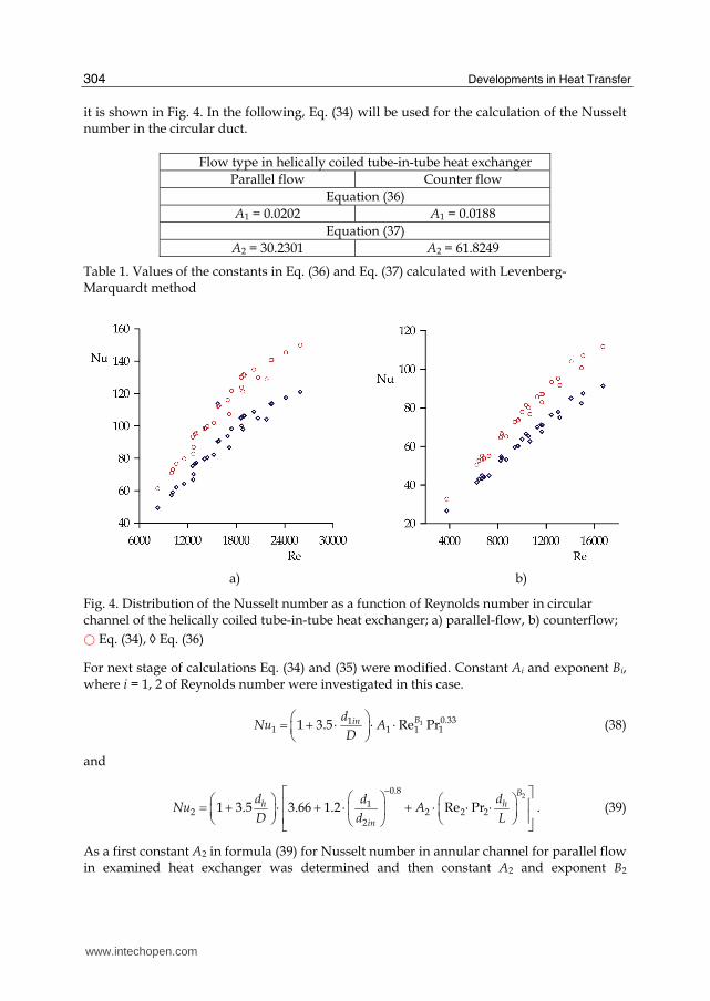
it is shown in Fig. 4. In the following, Eq. (34) will be used for the calculation of the Nusselt number in the circular duct.

Flow type in helically coiled tube-in-tube heat exchanger

Parallel flow Counter flow

Equation (36)

A1 = 0.0202 A1 = 0.0188

Equation (37)

A2 = 30.2301 A2 = 61.8249

Table 1. Values of the constants in Eq. (36) and Eq. (37) calculated with Levenberg-Marquardt method

a) b)

Fig. 4. Distribution of the Nusselt number as a function of Reynolds number in circular channel of the helically coiled tube-in-tube heat exchanger; a) parallel-flow, b) counterflow;

○ Eq. (34), ◊ Eq. (36)

For next stage of calculations Eq. (34) and (35) were modified. Constant Ai and exponent Bi, where i = 1, 2 of Reynolds number were investigated in this case.

1 0.3311 1 111 3.5 Re PrBind

Nu AD

⎛ ⎞= + ⋅ ⋅ ⋅⎜ ⎟⎝ ⎠ (38)

and

2

0.8

12 2 2 2

2

1 3.5 3.66 1.2 Re PrB

h h

in

d ddNu A

D d L

−⎡ ⎤⎛ ⎞⎛ ⎞ ⎛ ⎞⎢ ⎥= + ⋅ + ⋅ + ⋅ ⋅ ⋅⎜ ⎟⎜ ⎟ ⎜ ⎟⎢ ⎥⎝ ⎠ ⎝ ⎠⎝ ⎠⎣ ⎦. (39)

As a first constant A2 in formula (39) for Nusselt number in annular channel for parallel flow in examined heat exchanger was determined and then constant A2 and exponent B2

www.intechopen.com

Experimental Prediction of Heat Transfer Correlations in Heat Exchangers

305

simultaneously. During the calculations the flow in circular channel was described by formula (34). Identical calculations were carried out for Eq. (38), which was modified in order to adapt it to describe heat transfer in annular channel:

1 0.331 1 111 3.5 Re PrBhd

Nu AD

⎛ ⎞= + ⋅ ⋅ ⋅⎜ ⎟⎝ ⎠ . (40)

Also in this case as a first was calculated constant A1, and next constant A1 and exponent B1

in Eq. (40).

This procedure was to test, which of the equations will be better to map the set of

experimental data of the working fluid in annular channel – less complicated and correct in

case of turbulent flow – Eq. (34) or Eq. (35) describing the heat transfer for fluid flow in

laminar range.

( ) ( ) ( ) 20.82 1 2 2 2 21 3.5 3.66 1.2 Re Pr

Bh in hNu d D d d A d L

−⎡ ⎤= + ⋅ ⋅ + ⋅ + ⋅ ⋅ ⋅⎢ ⎥⎣ ⎦

A2 = 19.7433

A2 = 3.5754 B2 = 0.8229

( ) 1 0.331 1 111 3.5 Re PrB

hNu d D A= + ⋅ ⋅ ⋅

A1 = 0.0566

A1 = 0.0269 B1 = 0.8926

Table 2. Values of constant and exponents calculated with Levenberg-Marquardt for parallel flow in helically coiled tube-in-tube heat exchanger

a) b)

Fig. 5. Comparison of Nusselt number changes in annular channel (parallel flow) for Eqs. (39) and (40). Using Levenberg-Marquardt method was determined: a) one coefficient

and b) two coefficients , experimental points ◊

www.intechopen.com

Developments in Heat Transfer

306

In case when examined helically coiled tube-in-tube heat exchanger was working as a counter flow analogous calculations, using least squares method with modified Levenberg-Marquardt, were carried out to determine constants and exponents in correlation formulas for Nusselt number. Results are shown in Table 3 – forms of correlation formulas and determined values of the constants and exponents. Fig. 6. shows changes of two different formulas for Nusselt number as a function of Reynolds number in annular channel. Also in this case as a first was determined value of a constant, and as a second value of constant and exponent.

( ) ( ) ( ) 20.82 1 2 2 2 21 3.5 3.66 1.2 Re Pr

Bh in hNu d D d d A d L

−⎡ ⎤= + ⋅ ⋅ + ⋅ + ⋅ ⋅ ⋅⎢ ⎥⎣ ⎦

A2 = 25.397

A2 = 14.1959 B2 = 0.4997

( ) 1 0.331 1 111 3.5 Re PrB

hNu d D A= + ⋅ ⋅ ⋅

A1 = 0.0827

A1 = 0.3787 B1 = 0.6052

Table 3. Values of constant and exponents calculated with Levenberg-Marquardt for counter flow in helically coiled tube-in-tube heat exchanger

a) b)

Fig. 6. Comparison of Nusselt number changes in annular channel (counter flow) for Eqs. (38) and (39). Using Levenberg-Marquardt method was determined: a) one coefficient

and b) two coefficients , experimental points !

Analyzing changes of the Nusselt number in annular channel (hot fluid) shown on the Fig. 5a and Fig. 6a, drawn as dotted line, the best fit curves to experimental points can be noticed when the Levenberg-Marquardt method is used to determine values of two unknown parameters – constant and exponent in Eq. (39) than in case where only value of the one parameter was investigated.

www.intechopen.com

Experimental Prediction of Heat Transfer Correlations in Heat Exchangers

307

The differences between calculated values of constants and exponents in heat transfer correlation formulas for counterflow and parallel-flow configuration of the examined heat exchanger are result of the larger average temperature difference between the two fluids. Comparison of the Nusselt number changes with calculated one and two unknown parameters for turbulent (40) and laminar (39) form of the Nusselt formula leads to the conclusion that Eq. (40) better describes the kind of the fluid flows in annular channel for heat exchanger operating in parallel and counter flow.

4. Conclusion

In this paper methodology which allows for numerical determination unknown parameters in correlation formulas for Nusselt number and heat transfer coefficients on the hot and cold fluid side simultaneously was presented. Calculations were carried out on the basis of gathered experimental data for parallel and counter flow of working fluid in helically coiled tube-in-tube heat exchanger. The changes of Nusselt number in circular channel (turbulent flow) and annular channel (laminar flow) as a function of Reynolds number were presented also. Described methodology for determining constants and exponents in correlation formulas for Nusselt number can be used in designing of the different heat exchangers types and shapes of heat transfer surface.

5. References

Beck, J. V.; Blackwell, B.; Clair, Ch. R. St. (1985). Inverse Heat Conduction. Ill-posed Problems. John Wiley & Sons, ISBN 0-47-108319-4, New York, USA

Dean W.R. (1928). The Streamline Motion of Fluid in a Curved Pipe (second paper), Philos. Mag.,Vol. 7, pp. 673–695, ISSN 1941-5982

Dean, W.R. (1927). Note on the Motion of Fluid in a Curved Pipe, Philos. Mag., Vol. 4, pp. 208–223, ISSN 1941-5982

Fernández-Seara, J.; Uhía F.J.; Sieres, J.; Campo, A. (2007). A General Review of the Wilson Plot Method and its Modifications to Determine Convection Coefficients in Heat Exchange Devices. Applied Thermal Engineering, Vol.27, pp. 2745–2757, ISSN 1359-4311

Hewitt, G.F.; Shires, G.L.; Bott T.R. (1994). Process Heat Transfer. Begell House Publishers, ISBN 0-8493-9918-1, New York, USA

Holman, J.P. (2009). Heat Transfer. McGraw-Hill, ISBN 0-07-114320-3, New York, USA Ito, H. (1959). Friction factors for turbulent flow in curved pipes, Transactions of ASME D 81,

pp. 123-132, ISSN 0021-9223 Kumar, R.; Varma, H.K.; Agrawal, K.N.; Mohanty, B. (2001). A Comprehensive Study of

Modified Wilson Plot Technique to Determine the Heat Transfer Coefficient During Condensation of Steam and R-134a Over Single Horizontal Plain and Finned Tubes. Heat Transfer Engineering, Vol.22, pp.3–12, ISSN 0145-7632

Kumar, V.; Faizee, B.; Mridha, M.; Nigam, K.D.P. (2008). Numerical Studies of a Tube-in-Tube Helically Coiled Heat Exchanger. Chemical Engineering and Processing, Vol.47, pp. 2287–2295, ISSN 0255-2701

Kuppan, T. (2000). Heat Exchanger Design Handbook, Marcel Dekker, Inc, ISBN 0-8247-9787-6, New York, USA

Lawson, C.; Hanson R. (1995). Solving Least Squares Problems, ISBN 0-89871-356-0, Prentice Hall, Englewood Cliffs, USA

www.intechopen.com

Developments in Heat Transfer

308

Manglik, R.M. (2003). HeatTransfer Enhancement, In: Heat Transfer Textbook, A. Bejan and Kraus A.D., (Eds.), John Wiley & Sons, ISBN 0-471-39015-1, New York, USA

Nashchokin, V.V. (1980). Engineering Thermodynamics and Heat Transfer, Central Books Ltd, ISBN 0-71-471523-9, London, Great Britain

Pitts, D.R.; Sissom, L.E. (1998). Shaum’s Outline of Theory and Problems of Heat Transfer. McGraw-Hill, ISBN 0-07-050207-2, New York, USA

Press, W.H.; Teukolsky, S.A.; Vetterling W.T.; Flannery B.P. (1996). Numerical Recipes in Fortran 77: The Art of Scientific Computing. Cambridge University Press, ISBN 0-521-43064-X, New York, USA

Rennie, T.J.; Raghavan, V.G.S. (2006). Effect of Fuid Thermal Properties on the Heat Transfer Characteristics in a Double-Pipe Helical Heat Exchanger. International Journal of Thermal Sciences, Vol.45, pp. 1158–1165, ISSN 1290-0729

Rogers, G.F.C.; Mayhew Y. R. (1964). Heat Transfer And Pressure Loss In Helically Coiled Tubes With Turbulent Flow. International Journal of Heat Mass Transfer, Vol. 7, pp. 1207 – 1216, ISSN 0017-9310

Rose, J.W. (2004). Heat-Transfer Coefficients, Wilson Plots and Accuracy of Thermal Measurements. Experimental Thermal and Fluid Science, Vol.28, pp.77–86, ISSN 0894-1777

Schmidt, E.F. (1967). Wärmeübergang und Druckverlust in Rohrschlangen. Chemie Ingenieur - Technik, 39 Jahrgang, Heft 13, pp. 781 – 789, ISSN 0009-286X

Seban,. R.A.; McLaughlin, E.F. (1963). Heat Transfer in Tube Coils with Laminar and Turbulent Flow. International Journal of Heat Mass Transfer, Vol. 6, pp. 387 – 395, ISSN 0017-9310

Serth, R.W. (2007). Process Heat Transfer. Principles and Applications. Academic Press, ISBN 978-0-12-373588-1, Burlington, USA

Shah, R.K.; Joshi S.D. (1987). Convective Heat Transfer in Curved Ducts, In: Handbook of Single-Phase Convective Heat Transfer, S. Kakac, R.K. Shah and W. Aung (Eds.), ISBN 0-47-181702-3, John Wiley & Sons, New York, USA

Shilling, R.L; Bell, K.J.; Bernhagen, P.M.; Flynn, T.M.; Goldschmidt, V.M.; Hrnjak, P.S.; Standiford F.C.; Timmerhaus K.D. (1999). Heat-Transfer Equipment, In: Perry’s Chemical Engineers’ Handbook, R.H. Perry and Green D.W., (Eds.), McGraw-Hill, ISBN 0-07-049841-5, New York, USA

Shokouhmand, H.; Salimpour, M.R., Akhavan-Behabadi, M.A. (2008). Experimental Investigation of Shell and Coiled Tube Heat Exchangers Using Wilson Plots. International Communications in Heat and Mass Transfer, Vol.35, pp. 84–92, ISSN 0735-1933

Smith, E. M. (1997). Thermal Design of Heat Exchangers: A Numerical Approach: Direct Sizing and Stepwise Rating, and Transients, John Wiley & Sons, ISBN 0-47-001616-7, New York, USA

Sobota, T. (2011). Determinig of Convective Heat Transfer Coefficients in Heat Exchangers Using the Wilson Plot Technique, In: Thermal and Flow Proesses in Large Steam Boilers. Modeling and Monitoring, J. Taler, (Ed.), ISBN 978-83-01-16479-9, Warszawa, Poland (in Polish)

Viegas, R.M.C.M.; Rodríguez, M.; Luque, S.; Alvarez, J.R.; Coelhoso, I.M.; Crespo, J.P.S.G. (1998). Mass Transfer Correlations in Membrane Extraction: Analysis of Wilson-Plot Methodology. Journal of Membrane Science, Vol.145, pp.129-142, ISSN 0376-7388

Visual Numerics Inc. (2007). IMSL Fortran and C Application Development Tools, Vol. 1 and 2. Houston, Texas, USA

www.intechopen.com

Developments in Heat TransferEdited by Dr. Marco Aurelio Dos Santos Bernardes

ISBN 978-953-307-569-3Hard cover, 688 pagesPublisher InTechPublished online 15, September, 2011Published in print edition September, 2011

InTech EuropeUniversity Campus STeP Ri Slavka Krautzeka 83/A 51000 Rijeka, Croatia Phone: +385 (51) 770 447 Fax: +385 (51) 686 166www.intechopen.com

InTech ChinaUnit 405, Office Block, Hotel Equatorial Shanghai No.65, Yan An Road (West), Shanghai, 200040, China

Phone: +86-21-62489820 Fax: +86-21-62489821

This book comprises heat transfer fundamental concepts and modes (specifically conduction, convection andradiation), bioheat, entransy theory development, micro heat transfer, high temperature applications, turbulentshear flows, mass transfer, heat pipes, design optimization, medical therapies, fiber-optics, heat transfer insurfactant solutions, landmine detection, heat exchangers, radiant floor, packed bed thermal storage systems,inverse space marching method, heat transfer in short slot ducts, freezing an drying mechanisms, variableproperty effects in heat transfer, heat transfer in electronics and process industries, fission-trackthermochronology, combustion, heat transfer in liquid metal flows, human comfort in underground mining, heattransfer on electrical discharge machining and mixing convection. The experimental and theoreticalinvestigations, assessment and enhancement techniques illustrated here aspire to be useful for manyresearchers, scientists, engineers and graduate students.

How to referenceIn order to correctly reference this scholarly work, feel free to copy and paste the following:

Tomasz Sobota (2011). Experimental Prediction of Heat Transfer Correlations in Heat Exchangers,Developments in Heat Transfer, Dr. Marco Aurelio Dos Santos Bernardes (Ed.), ISBN: 978-953-307-569-3,InTech, Available from: http://www.intechopen.com/books/developments-in-heat-transfer/experimental-prediction-of-heat-transfer-correlations-in-heat-exchangers

© 2011 The Author(s). Licensee IntechOpen. This chapter is distributedunder the terms of the Creative Commons Attribution-NonCommercial-ShareAlike-3.0 License, which permits use, distribution and reproduction fornon-commercial purposes, provided the original is properly cited andderivative works building on this content are distributed under the samelicense.