Tampereen teknillinen yliopisto. Julkaisu XXX Tampere University of Technology. Publication XXX Toni Huovinen Independent Component Analysis in DS-CDMA Multiuser Detection and Interference Cancellation Preliminary Examination Edition Thesis for the degree of Doctor of Technology to be presented with due permission for public examination and criticism in Tietotalo Building, Auditorium TBXXX, at Tampere University of Technology, on the XX-th of xxxxxx 2008, at 12 noon. Tampereen teknillinen yliopisto - Tampere University of Technology Tampere 2008
Multiuser detection (MUD) and interference cancellation (IC) have emerged asimportant theoretical and practical problems among spread spectrum multipleaccess researchers during the last decades. Conventionally, MUD and IC meth-ods are based on second order statistics. They assumes low statistical correlationbetween desired signal components and interfering ones. One relative new ideais to use also higher order statistics (HOS) to improve the system performance.Especially, HOS based blind source separation (BSS) techniques are attractive,since they are able to separate signals from a mixture of original source signalsin a completely blind manner, i.e., without explicit knowledge of signals wave-forms. Consequently, many types of interference sources, for instance, internalinterferences due to multiple access and non-Gaussian external interference sig-nals, can be suppressed out. However, possible performance gains due to BSSor HOS processing, in general, compared to conventional second order methodsare not studied extensively in the literature – until this PhD dissertation.
In this dissertation, the main emphasis is on BSS assisted MUD and ICmethods and, especially, on those which employ an independent componentanalysis (ICA). Advanced MUD/IC strategies are considered and applied in di-rect sequence code division multiple access (DS-CDMA) uplink receivers. Inparticular, a new family of BSS/ICA assisted successive interference cancel-lation (SIC) schemes are introduced and performance of such a receivers areset against to conventional methods. The main emphasis is on the overcom-plete data which situation arises in challenging highly loaded systems. The newreceiver structures combine the main benefits of HOS signal processing and con-ventional non-linear MUD methods, that is, (i) inherent mitigation of varioustypes of interference sources by BSS/ICA, (ii) robustness against parameter es-timation errors due to BSS/ICA, (iii) greatly improved interference suppressioncapability due to novel combination of SIC ideology and BSS/ICA.
This dissertation consists of one journal article, nine conference articles and oneresearch repot listed in the following:
[P1] T. Huovinen and T. Ristaniemi. Comparison of nonlinear interferencecancellation and blind source separation techniques in the DS-CDMAuplink. In Proc. 14th IEEE Symposium on Personal, Indoor and MobileRadio Communications (PIMRC’03), pages 989–993, September 2003.
[P2] T. Huovinen and T. Ristaniemi. Effect of channel estimation and mul-tipath on interference cancellation employing blind source separation inthe DS-CDMA uplink. In Proc. 2004 IEEE 59th Vehicular TechnologyConference(VTC’04-Spring), pages 1494–1498, May 2004.
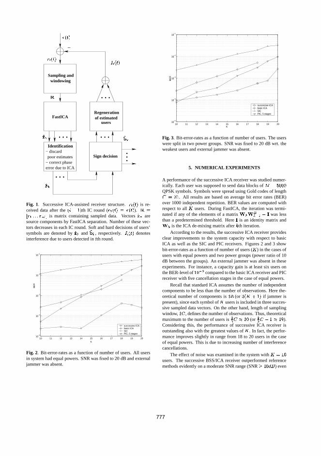
[P3] T. Huovinen and T. Ristaniemi. Blind source separation based successiveinterference cancellation in the DS-CDMA uplink. In Proc. 2004 IEEEFirst International Symposium on Control, Communications and SignalProcessing (ISCCSP’04), pages 775–778, March 2004.
[P4] T. Huovinen and T. Ristaniemi. DS-CDMA capacity enhancement usingblind source separation based group-wise successive interference cancella-tion. In Proc. 2004 IEEE 5th Workshop on Signal Processing Advancesin Wireless Communications (SPAWC’04), pages 184–188, July 2004.
[P5] T. Ristaniemi and T. Huovinen. Joint delay tracking and interferencecancellation in DS-CDMA using successive ICA for oversaturated data. InProc. 5th International Conference on Independent Component Analysisand Blind Signal Separation (ICA’04), pages 1173–1180, September 2004.
[P6] T. Huovinen and T. Ristaniemi. Independent component analysis us-ing successive interference cancellation for oversaturated data. EuropeanTransactions on Telecommunications, 17(5):577–589, 2006.
[P7] K. Raju, T. Huovinen, and T. Ristaniemi. Blind interference cancellationschemes for DS-CDMA systems. In Proc. 2005 IEEE/URSI InternationalSymposium on Antennas and Propagation, pages 73–76, July 2005. invitedpaper.
[P8] T. Ristaniemi and T. Huovinen. Joint multipath delay tracking and in-terference cancellation in DS-CDMA systems using successive ICA foroversaturated data. In Proc. 2006 IEEE 1st International Symposium onWireless Pervasive Computing (ISWPC’06), pages 1–5, January 2006.
[P9] T. Huovinen, A. Shahed hagh ghadam, and M. Valkama. Blind diver-sity reception and interference cancellation using ICA. In Proc. 2007IEEE International Conference on Acoustics, Speech and Signal Process-ing (ICASSP’07), pages 685–688, April 2007.
[P10] A. Shahed hagh ghadam, T. Huovinen, and M. Valkama. Dynamic off-set mitigation in diversity receivers using ICA. In Proc. 18th IEEESymposium on Personal, Indoor and Mobile Radio Communications(PIMRC’07), pages 1–5, September 2007.
[P11] T. Huovinen, A. Shahed hagh ghadam, and M. Valkama. Higher-orderblind estimation of generalized eigenfilters using ICA. Tampere Univer-sity of Technology. Department of Communication engineering. ResearchReport 2008:1, 1:1–14, 2008.
Other Publications of the Author
The author of this thesis has also published (or submitted) the following threearticles which are not included in this dissertation:
1. T. Huovinen, A. Shahed hagh ghadam and M. Valkama. “Higher-orderblind estimation of generalized eigenfilters using Independent ComponentAnalysis,” in Proc. IEEE/IARP CIP2008, 2008, submitted.
2. T. Huovinen, E. Pajala and T. Ristaniemi. “On the analytic perfor-mance of differential spread spectrum code acquisition,” in Proc. IEEEICCS2006, 2006.
3. E. Pajala, E. S. Lohan, Toni Huovinen and Markku Renfors. “Enhanceddifferential correlation method for the acquisition of galileo signals,” inProc IEEE ICCS2006, 2006.
:= Definition (left hand side is defined by right one)(·)† Pseudo inverse of a matrix(·)∗ Complex conjugate(·)T , (·)H Matrix transpose and Hermitian transpose| · | Absolute value‖ · ‖ Euclidean norm0, 0n Origin (n-dimensional vector of zeros)β = [b1, ..., bK ]T Vector of user symbolsδk, δkl Delay Estimation Error∆ = diag(a1, . . . , aK) Diagonal matrix of channel coefficientsΓ Code cross-correlation matrixη(t) Additive noise signalη Additive noise vectorη, η Noise in MF output(s)θ(k, k′) Correlation for user identificationΛ Eigenvalue matrix of ICA observations or received dataξk(·) Spreading code sequence of the k-th userρkl Cross-correlation between k-th and l-th userskl, kl, kl
Correlations between asynchronous users’ spreadingcodes
σ2 Noise varianceΣ Noise covariance matrixτk, τkl, τkl Delay of the k-th user’s l-th path and its estimate
Υk, Υk Multiaccess interference component and its estimate
Υext(t), Υext[m] External interference signalΨ(v) Update term of EASI algorithmΩK(·) Contrast function of jointly optimum MUDı Imaginary unitak, akl Path coefficient of k-th user’s l-th pathA ICA mixing matrixbk, bk[m] (m-th) symbol of k-th userb Vector containing “early”, “middle” and “late” symbols
of all users
B, B De-mixing matrix and its estimate(ci)
∞i=1 Binary chip sequence
C Number of chips per symbolCx Covariance matrix of ICA observationsCr Covariance matrix of received data vectorC Set of complex numbersen M-GEF vectorEs Principal eigenvector matrix of CE (·) Expected valuef : R→ R ICA nonlinearity (derivative of F )F : R→ R ICA contrast functiongk, gk One column of matrix G and its estimate
G, G Code matrix after propagation channel and its estimatehn Column of a mixing matrixI Identity matrixℑ· Imaginary part of complex numberJ Number of ICA observationsK Number of usersL Number of pathsM Number of symbol in one frame or blockN Number of ICA sourcesmk, mk LMMSE transformation of k-th (user) component and
its estimateM0 LMMSE matrixO(·) Order ofpTc
(t) Chip wave formP Number of PIC stagesP (·) Probability measure
Q(·) Q-function, i.e., a complementary cumulative distribu-tion function (CDF) of the unit variance normal randomvariable
r(t) Received signalr Received (stochastic) data vector of length 2Cr[m] m-th sample r (contains contributions m-th symbols)Rn Observation covariance of desired componentR′
n Observation covariance of interference and noiseR Set of real numbersℜ· Real part of complex numbers = [s1, s2, . . . , sN ]T ICA source component vectorsn ICA source componentsign(·) Sign-functionT Symbol durationTc = T/C Chip durationU Arbitrary unitary matrixV Whitening transformationz Whitened ICA observation vectorwi Whitened ICA basis vectorW Whitened ICA mixing matrixxi ICA observationx = [x1, x2, . . . , xM ]T ICA observation vectoryk, yk[m] Matched filter outputy = [y1, y2, . . . , yK ] Vector of matched filter outputsyDD Soft output of decorrelating detectoryLMMSE Soft output of LMMSE-detector
Abbreviations
AWGN Additive White Gaussian NoiseBEP Bit Error ProbabilityBER Bit Error RateBPSK Binary Phase Shift KeyingBSS Blind Source SeparationCDF Cumulative Distribution FunctionCDMA Code Division Multiple AccessDD Decorrelating DetectorDS Direct Sequence
Code division multiple access (CDMA) is a multiplexing technique, which en-ables multiple users to access simultaneously and asynchronously to a commonradio frequency (RF) channel by modulation and spreading of the information-bearing signals with a user-specific spreading sequences or spreading codes. Forexample, third generation’s mobile communication systems as well as manyother latest radio systems are based on the CDMA technology. In addition,CDMA or some of its variants are good candidates for multiplexing techniquealso in future commercial systems, since they fit well to increasing demand forhigher bit rates. Different ways to spread the signal over a wide and commonfrequency band results in different multiple access schemes. Direct sequence(DS) and frequency hopping (FH) (and hybrids of them) are examples of single-carrier modulation schemes, and have been under extensive research [89, 113].The WCDMA standard, for instance, is based on DS-modulation [42]. Also inthis dissertation, we study CDMA systems where spreading is carried out byDS-modulation.
An inherent capability to resist interference is the most important featureof spread spectrum communication – and, thus, also of CDMA. As a matterof fact, the concept of spread spectrum communication was originally intro-duced particularly for military communication and especially for antijammingpurposes [93]. Later, the spread spectrum techniques were harnessed to the
civilian use. For example, a possibility to use the spread spectrum system ontop of traditional narrowband systems without causing insuperable interferenceincrement is very fascinating in the commercial communication where RF bandhas become scarce resource [92]. Nevertheless, also CDMA systems – like anyradio communication systems – are interference limited. Furthermore, in prac-tise, also an internal multiple access interference (MAI) due to the non-idealcross-correlations between users’ spreading sequences limits the performance ofa CDMA system. Conventionally, this interference is considered as an additionalbackground noise which increases a total noise floor and, eventually, makes con-ventional detectors inadequate in highly loaded systems. Conventional detectionis also quite sensitive to external interference sources like adjacent channel in-terference or jamming which has lead to development of numerous interferencerejection techniques. An effective interference suppression or cancellation (IC)is a natural way to enhance system performance.
In CDMA literature (see, e.g., [89, 112, 113]), MAI reduction is often calledas multiuser detection (MUD). In it, the existence of the interfering users istaken into account when detecting the desired user(s), unlike in conventionalsingle-user detection. Conventional MUD/IC methods are typically based onsecond order statistical properties of data, hence, being founded on low statis-tical correlation assumption between desired signal components and interferingones. One relative new idea is to use higher order statistics (HOS), whichmakes the methods very robust against problems related to incomplete cross-correlation properties and also against a near-far problem (i.e., differences inreceived power) which is an another limiting factor for conventional detectionand IC. Especially, HOS based blind source separation (BSS) techniques [29,53]are attractive, since they are able to separate signals from a mixture of originalsource signals in a completely blind manner, i.e., without explicit knowledge ofwaveform structure (modulation) or mixing coefficients. Consequently, manytypes of interference sources, for instance, internal interferences due to multipleaccess and out-of-cell interferences (intentional and unintentional) due to cellu-lar network, can be mitigated in DS-CDMA systems. Here, our main emphasisis particularly in BSS assisted MUD. In addition, we also touch the externalinterference suppression briefly.
1.2 Scope of the Dissertation
In this dissertation work, the goal is to study possible benefits of using higherorder statistics in DS-CDMA multiuser detection and interference cancellation.
This is carried out study by developing new non-linear MUD/IC method whichemploy HOS based BSS and comparing their performance to existing MUDmethods. The main emphasis is on the asynchronous uplink (mobile-to-base)reception and, especially, on highly loaded systems which means in DS-CDMAthat the number of active connections or users is high compared to number ofchips per bit being used, that is, to a processing gain of the system. FromBSS’s point of view, the highly loaded system model appears to correspondto so called “more sources than sensors” -problem [53], which is considered achallenging problem in literature.
Novel successive interference cancellation (SIC) schemes obeying the fun-damental procedures of conventional SIC [43, 112], are proposed. That is tosay, (i) the estimation of interference, (ii) re-generation of interference and fi-nally (iii) subtraction of the re-generated interference from the original data.What makes the schemes advanced compared to conventional SIC is the wayof estimating the interference using HOS based BSS by means of independentcomponent analysis (ICA) [22, 53] and a sensitive selection of the interferencesources to be subtracted. The proposed receiver structures combine the mainbenefits of BSS/ICA and conventional SIC methods:
• inherent mitigation of various types of interference sources by BSS/ICA,
• robustness against parameter estimation errors due to BSS/ICA,
• greatly improved interference suppression capability in highly loaded sys-tems due to novel combination of SIC ideology and HOS signal processingof BSS/ICA.
Best of all, all the benefits are achieved using single receiver antenna only.Notice also that the last item in the list above can also be seen as a way tosomewhat circumvent the “more sources than sensors” -problem of BSS/ICA.
Noisy models have been an another challenge in BSS/ICA area [53]. Inmost of practical applications, nevertheless, the presence of an additive back-ground noise can not be neglected. Especially in telecommunications, somelevel of Gaussian noise is always interfering the reception. For this reason, thisdissertation study considers also the noisy ICA problem. It is shown that con-ceptually many basic ICA algorithms designed for noise-free ICA models, canactually provide the best linear source separation solution possible in terms ofinput-output signal-to-interference-and-noise (SINR) gain. This seems not tobe well-understood in the literature earlier. From CDMA reception perspec-tive, this founding means that the performance of BSS/ICA assisted receptionis indeed exceedingly competitive against any suboptimum MUD detector.
One should also recognize the fact that in interference subtractive receivers(in SIC, for example), a very precise channel state information is needed inthe interference subtraction to prevent interference enhancement. This is whyaccurate code acquisition and tracking is of great importance. However, an im-portant property of BSS/ICA is its inherent capability to cope with erroneoustiming estimates. This feature of BSS/ICA is exploited to refine tentative tim-ing estimates after the ICA processing, but before interference re-generation andsubstraction, such that also the timing refinement procedure takes advantageof interference suppression due to blind separation. Consequently, the require-ment of extremely precise code tracking can be relaxed in the proposed ICA-SICschemes. This kind of relaxation is not inherently possible in conventional in-terference subtractive receivers.
1.3 Outline and Organization
This PhD dissertation consists of two parts. The first part gives an introductionand background knowledge of the research area to which the topic of the dis-sertation work belongs. Also the earlier literature on the area is reviewed. Thesecond part is a compilation of eleven original research publications reportingthe novel scientific contributions of this dissertation work in detailed manner.In the first part, these publications are referred as [P1–P11].
Rest of the first part is organized as follows. In Chapter 2 we describe basicsof DS-CDMA systems starting with definitions of different system models andcontinuing with description of conventional single-user detection. In Chapter 3,we discuss the central signal processing method of this dissertation, indepen-dent component analysis (ICA). We give definition of ICA, reveal the connectionbetween ICA and DS-CDMA models and review the most well known ICA al-gorithms. In the end of the chapter, we discuss on performance of the ICAalgorithms. In Chapter 4, we deal with multiuser detection (MUD). We sum-marize the basics of optimum and suboptimum MUD as well as blind MUD.The former includes also the ICA assisted MUD. In Chapter 5, we discuss therejection of external interference. Finally, in Chapters 6 and 7, we give summaryof the publications and draw a conclusions of the work, respectively.
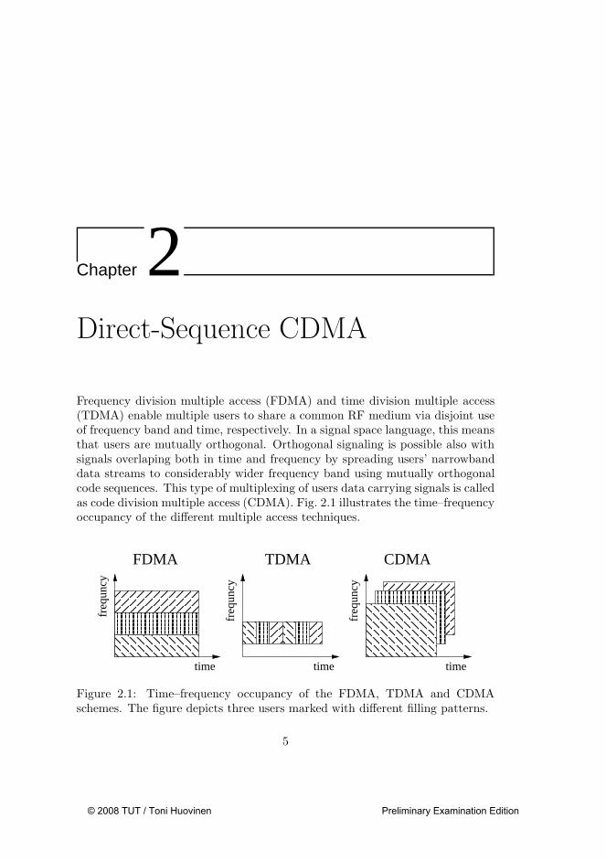
Frequency division multiple access (FDMA) and time division multiple access(TDMA) enable multiple users to share a common RF medium via disjoint useof frequency band and time, respectively. In a signal space language, this meansthat users are mutually orthogonal. Orthogonal signaling is possible also withsignals overlaping both in time and frequency by spreading users’ narrowbanddata streams to considerably wider frequency band using mutually orthogonalcode sequences. This type of multiplexing of users data carrying signals is calledas code division multiple access (CDMA). Fig. 2.1 illustrates the time–frequencyoccupancy of the different multiple access techniques.
freq
uncy
time time
freq
uncy
freq
uncy
time
FDMA TDMA CDMA
Figure 2.1: Time–frequency occupancy of the FDMA, TDMA and CDMAschemes. The figure depicts three users marked with different filling patterns.
Figure 2.2: DS-modulation of BPSK symbols (baseband). T and Tc denotessymbol and chip durations, respectively. Modulated data signal is point-wise(in time) product of the binary data and spreading sequence signals.
In Direct sequence (DS-) CDMA the spreading is carried out by direct modu-lation of the information bearing signals with a user-specific wideband signaturesequences or codes. The principle is shown for BPSK symbols (that is, sym-bols having values in −1, 1) in Fig. 2.2. The main benefit of the DS-CDMAis that the strict orthogonality between the signature sequences, and hence,also between users’ data bearing signals, can be relaxed. E.g., the performanceof the simple de-modulator is degraded in the presence of non-orthogonal in-terfering users, but the degradation can be kept in tolerable levels providedthat cross-correlations between users are moderate. Relaxing the orthogonalityrequirement makes DS-CDMA even more attractive as a multiple access tech-nique. For instance, users can access the system asynchronously and unlikein strictly orthogonal multiple access schemes (such as TDMA and FDMA), itis possible to trade off reception quality for increased capacity. However, dueto multiaccess interference, additional interference mitigation or multiuser de-tection (MUD) techniques are usually needed to improve system performance.These techniques are the main theme of this dissertation.
Rest of this chapter introduces the principle of DS-CDMA more in detail.First, in Section 2.1, we present the short-code DS-CDMA system model which
we then study in the rest of the dissertation. In Section 2.2, we introduce aprinciple of conventional single-user detection (SUD) which is based on spread-ing code matched filtering. In addition, we define a multiple access interferenceexperienced by conventional detector. Finally, in Section 2.3, we discuss shortlyon code synchronization.
2.1 Signal Model
Next, we present the complex-valued baseband model of the carrier modulatedshort-code DS-CDMA signal. This model is commonly used in literature andalso assumed in [P1–P8]. Let us assume that system has K active users allsending a symbol, bk, drawn randomly from some predetermined, unit-energy,complex-valued symbol constellation, over a radio-frequency channel with ad-ditive white Gaussian noise (AWGN). Then we write the received multiuserDS-CDMA signal, in its’ simplest form, as [112]
r(t) =
K∑
k=1
akbkξk(t) + η(t), t ∈ [0, T ) (2.1)
where T is a symbol duration, ak ∈ C is a complex path gain of the k-thuser and ξk(·) denotes the pseudo-random spreading code wave associated withthe k-th user. We adopt here the typical assumption made in the theoreticalliterature that the code waveforms are supported by the time interval [0, T ).Under this assumption the system characterized by the model (2.1) do not haveintersymbol interference. We also assume that the code waves have unit energy,
i.e.,∫ T
0 ξk(t)2dt = 1. In addition, η(t) denotes an additive white Gaussian noisesignal.
A proper selection of spreading codes has an important role in the elabora-tion of DS-CDMA systems. Properties of the codes affect directly on system’scapability to prevent active users from interfering one another too much, aswell as, to cope with multipath propagation. Basically, cross-correlations or aninnerproducts between pairs of code waves, that is,
ρkl := 〈ξk, ξl〉 =
∫ T
0
ξk(t)ξl(t)dt, (2.2)
measure system’s inherent multiaccess interference resistance. Ideally, ρkl ≈ 0for k 6= l. Correspondingly, an autocorrelation function of a code wave charac-terizes the ability to cope with multipaths. If the correlation between any two
different phases of any code is small (close to zero), the system is able to resistmultipath propagation inherently. [95, 112]
Usually the code wave is formed by modulating a so called chip wave, pTc,
antipodally with a binary code sequence (ci)∞i=1, i.e., [113]
ξ(t) =C∑
i=1
(−1)cipTc(t − (i − 1)Tc) (2.3)
where C is the spreading factor and Tc = T/C is the chip “duration”. Inpractice, the chip waves do not have to be strictly time-limited, but they arerequired to satisfy the condition
∫ ∞
−∞
pTc(t)pTc
(t − nTc)dt = 0, (2.4)
for all n ∈ 1, 2, . . .. Two theoretical examples of such waveforms are a rect-angular pulse,
pTc(t) =
1 , if 0 ≤ t < Tc
0 , otherwise, (2.5)
and sinc-pulse,
pTc(t) = sinc
(2t
Tc− 1
). (2.6)
These are examples of time-limited and bandwidth-limited waves, respectively.In practice, some compromise of these two are selected due to the achievedspectral efficiency. For example, raised cosine with parameter 0 ≤ β ≤ 1,
pβ(t) = sinc
(t
Tc
)cos (βπt/Tc)
1 − (2βt/Tc)2(2.7)
has a band-width (1 + β)/(2Tc) [95].The simple DS-CDMA model (2.1) is so called (symbol) synchronous model.
It means that wide-band symbols of each user are assumed to arrive to the re-ceiver exactly at the same time. Consequently, it is sufficient to consider onlythe reception of one symbol (per user) at a time. This approach is valid mainlyin the downlink communications where the base station transmits the signalsof all users in the system. Thus, the synchronization of transmissions is easyto implement. In the uplink, in turn, each active user sends its data indepen-dently and, in addition, they all have own, more or less random, propagationdelays. For this reason, we need also an asynchronous signal model. The model
must take into account a block or a frame of, say, M symbols, since due toasynchronism the demodulation of a particular users symbol is now affected bymore than one symbol of the other users. Hence, we write the asynchronousDS-CDMA model as [112]
r(t) =
K∑
k=1
M∑
m=1
akbk[m]ξk(t − mT − τk) + η(t). (2.8)
Here, τk ∈ [0, T ) defines a (relative) propagation delay and bk[m] the m-thsymbol for k-th user. We assume that the users are in ascending order withrespect to their delays, i.e., that τ1 ≤ τ2 ≤ . . . ≤ τK . This assumption simplifiessome following notations and has no effect on generality. Further, we actuallyassume in (2.8) that the reception of each user’s data block is beginning (as wellas ending) within one symbol duration T .
In practice, the receiver observes several reflections of the transmitted signal.They all have traveled different radio paths and, hence, have different path gainsand, especially, propagation delays [95,113]. In the case of L propagation paths,we write the asynchronous (multipath) DS-CDMA model as [113]
r(t) =
K∑
k=1
M∑
m=1
bk[m]
L∑
l=1
aklξk(t − mT − τkl) + η(t), (2.9)
where akl ∈ C and τkl are the complex path gain coefficient and the propagationdelay for the l-th path of the k-th user, respectively. The delays of each path isassumed to be within one symbol duration T . The model 2.9 is often referredas “fixed multipath” model.
2.2 Conventional Single-User Detection
Let us consider, first, a so called single-user channel model, [112, 113]
r(t) = abξ(t) + η(t), t ∈ [0, T ), (2.10)
that is, the model (2.1) with one user (K = 1). We define the (coherent)matched filter (MF) output as
is Gaussian random variable with zero mean and variance σ2. The MF output,y, is sufficient statistics to achieve the minimum probability of error when de-tecting the transmitted symbol b [95,112]. More precisely, the minimum distancedecision after MF results in the minimum bit error probability (BEP) amongall detectors given that noise realizations are not known. The error probabilityof such detector is given as [112]
BEP = Q
(|a|2
σ
), (2.13)
where Q(·) is a complementary CDF of the unit variance and zero mean Gaus-sian random variable. This sets the unified upper bound for the system perfor-mance of any DS-CDMA receiver, and is called as the single-user bound. TheMF detector is also called as the conventional single-user detector (SUD).
Let us turn our attention to the synchronous K-user channel model (2.1).The output of the k-th user matched filter is now, [112,113]
yk = a∗k〈ξk, r〉 = a∗
k
∫ T
0
ξk(t)r(t) dt (2.14)
= |ak|2bk + a∗
k
∑
j 6=k
ajbjρjk + ηk (2.15)
where ηk is the filtered Gaussian noise term defined analogously to (2.12), andρjk is the cross-correlation between the signature waveforms. The sum termin (2.15) is multiaccess interference (MAI) affecting on detection of k-th user.If signature waves, ξk, k = 1, . . . , K, are orthogonal, i.e., ρjk = 0 ∀j 6= k,the MAI term vanishes, and yk equals to single-user MF output for all users.Consequently, the MF detector is optimum (in the sense that it minimizes BEP)also in the orthogonal multiuser system. In general, the MAI term naturallydeteriorates the detection compared to single-user bound, and the MF output,yk, is not any more the sufficient statistics to minimize the bit error probability[112].
Multiaccess interference affecting on the conventional single-user receptiongets more complicated in asynchronous multiuser channel (2.1). Assuming weknow the propagation delay, τk, we define the MF output for k-user’s m-th
where Υk[m] is a MAI term. Before characterizing this term rigorously, we defineso called asynchronous cross-correlations between the signature waveforms asfollows:
kl :=
∫ ∞
−∞
ξl(t + T − τl)ξk(t − τk) dt, (2.17)
kl :=
∫ ∞
−∞
ξl(t − τl)ξk(t − τk) dt and (2.18)
kl
:=
∫ ∞
−∞
ξl(t − T − τl)ξk(t − τk) dt. (2.19)
These correlations in a sense determines how the current (e.g., m-th) symbol ofthe k-th user is affected, respectively, by the preceding ((m−1)-th), the current(m-th) and the succeeding ((m + 1)-th) symbols of the l-th user. Notice, that
kl = 0 when τl < τk and
kl
= 0 when τl > τk.(2.20)
Now, assuming τ1 ≤ τ2 . . . ≤ τK we can write the multiaccess interference termin (2.16) as
Υk[m] =∑
l<k
(albl[m]kl + albl[m + 1]
kl
)
+∑
l>k
(albl[m − 1]kl + albl[m]kl) .(2.21)
Not only the correlations kl, kl and kl
but also the complex path gaincoefficients ak, k = 1, 2, . . . , K, affect on the multiaccess interference, Υk[m],in (2.21). If the coefficients have clearly different moduli, the users with smallmoduli suffer from the effect of the multiaccess interference more than the userswith relatively large moduli [112]. This situation appears especially in DS-CDMA uplink due to the spatial diversity of transmitting users. If all userstransmit their signals with equal powers, then for example the users that are far
from the base station are received with weaker powers than the users close tothe base station. This negative effect of the path gain coefficients with differentmoduli, or in other words the users with different received powers, is called asnear-far problem.
Finally, we consider the conventional SUD in multipath channel (2.9). Inmany radio techniques multipath phenomenon and especially a fading phe-nomenon caused by it deteriorates the performance of the system [95]. However,as already discussed in the previous section, good autocorrelation properties ofusers’ spreading codes makes the DS-CDMA systems to resist distortion due tomultipath propagation. Basically, this means that low correlations between codephases pushes down the contribution due to interfering multipath componentsin MF output. Naturally, code autocorrelation can never be fully ideal (i.e., zeroautocorrelation between any miss-aligned code phases) in practice and, hence,existence of multipath interference increases the interference floor also in singleMF output. A RAKE receiver [113] is an extension of the conventional detectorwhich can take diversity advantage of the multipath environment. The RAKEreceiver of k-th user consists of several MF detectors that are matched to codephases of different paths. These MF branches are often called as fingers. RAKEreceiver combines finger outputs, say ykl[m], l = 1, . . . , L, e.g., according toprinciple of maximal ratio combining (MRC) [95], that is,
y′k[m] =
L∑
l=1
a∗klykl[m]. (2.22)
This improves a signal-to-noise(or interference)-ratio and, by this way, also thesystem performance.
2.3 On Code Synchronization
Conventional matched filter detection (and also most of the existing more anadvanced detection methods) requires accurate knowledge of users’ propagationdelays or, more precisely, (temporal) phase of the spreading sequences of decidedusers. We denoted this quantity earlier by τk (or τkl in the multipath context).Typically DS-CDMA receivers consist of two code synchronization or delay es-timation stages: acquisition stage and delay tracking stage [113]. The purposeof acquisition is to obtain a coarse pre-estimate of the delays in precision ofroughly a half chip duration. Code tracking then refines this pre-estimate andalso adapts to a possible slow fluctuation in delay after the acquisition stage.
Describing details of these two code synchronization stages is out of scopein this dissertation. However, we assume in the following that the acquisitionis performed, i.e., that receivers know coarse delay estimates for all desiredusers (and propagation paths), and denote the estimates by τk (or τkl), k =1 . . .K. In addition, we denote the delay estimation errors by δk := τk − τk (orδkl := τkl − τkl) and assume that |δk| (or |δkl|) < 1/2 for all k ∈ 1 . . .K (andl ∈ 1 . . . L).
Further, we can assume that acquisition is performed in discrete time (dig-ital) domain and that the received continuous time signal is, first, sampledby chip matched filter. Consequently, resolution of code acquisition is onechip duration and, thus, τk = dkTC (and τkl = dklTC) for some integer(s)dk (and dkl) ∈ 1, . . . , C.
Before moving to more advanced DS-CDMA reception principles, let us takea look at the central signal processing method of this thesis, namely at inde-pendent component analysis (ICA) [29, 52, 53]. ICA is a statistical method forsearching independent source random variables or signals from a set of observedlinear combinations of them. (In this dissertation we consider only linear ICA.)One of the main applications of ICA is blind source separation (BSS), which hasbecome an attractive field of research in statistical signal processing and neuralnetwork communities. ICA performs purely in a blind manner, i.e., without anyexplicit knowledge of original source variables or a mixing transformation. Itrelies on assumption of statistical independency of sources. Although indepen-dency is a very strong assumption from a theoretical point of view, it is oftenquite a realistic assumption in practice. Consequently, ICA has drawn a lot ofattention in various application fields lately.
The idea of ICA was first introduced in a neurophysiological setting in theearly 1980s by researchers (J. Herault, C. Jutten and B. Ans) who needed a blindmethod to separate the neural impulses coming from different parts of the humanbody [5,40,41]. Later on, ICA has been studied and applied in several very dif-ferent signal processing contexts like in audio and biomedical signal processing,feature extraction, finance, seismology, etc. Telecommunications related appli-cations of ICA have been found earlier, e.g., in MIMO systems [62,101,117,118],I/Q processing receivers [107], DS-CDMA blind multi-user detection [98] andDS-CDMA out-of-cell interference cancellation [9,96,97]. More inclusive review
of history of ICA and applications using ICA is given, e.g., in [53, 56, 57].
In this chapter, we first give a definition of linear ICA (Section 3.1). Next,in Section 3.2, we show that DS-CDMA model actually equals readily to ICAmodel. Then we continue by reviewing different algorithms briefly (Section 3.3)and, finally, discussing on performance issues of ICA algorithms (Section 3.4).
3.1 Definition
In this dissertation, we cover only, so called, linear independent componentanalysis, which we define in this section. Also other, extended, forms of ICAis known in literature (see, e.g., definitions of convolutive ICA and non-linearICA in [53]). In the following, we give definitions for the basic noise-free (linear)ICA, noisy (linear) ICA and (linear) ICA with overcomplete basis in Sections3.1.1, 3.1.2 and 3.1.3, respectively.
3.1.1 Basic Noise-Free ICA
Prior to giving the definition of basic independent component analysis, we needto introduce the generative ICA model. In literature, the ICA model was firstgiven for real-valued data and mixtures [22] and later on generalized straight-forwardly for the complex-valued case. Here, we present the complex-valuedmodel since it coincides with DS-CDMA data model defined earlier as will beseen in Section 3.2. Let s = [s1, s2, . . . , sN ]T be a random vector, such that com-ponents s1, s2, . . . and sN are mutually independent, non-Gaussian, complex-valued random variables – to be precise, one and only one of them is allowed tobe Gaussian. Further, let A = [h1 h2 . . .hN ] ∈ CJ×N be a constant complex-valued mixing matrix which we assume to have a full column rank. The columnvectors, h1 h2 . . .hN , are called as ICA basis vectors. Now, the basic noise-freeICA model is defined simply as linear model,
x = As, (3.1)
in which x = [x1, x2, . . . , xJ ]T is the observed J-dimensional random vector.The components of the vector s and x are called as independent components andICA observations, respectively. Notice, that we assume above that the numberof linear combinations xi is greater or equal than the number of independentcomponents si (J ≥ N). In other words, it means that there is at least as manyobservations as sources.
Now we define independent component analysis as estimating independentcomponents s1, s2, . . . , sN and mixing matrix A from model (3.1) while only thevector x is known. In other words, the goal is essentially to invert the model(3.1) blindly, that is, to find a de-mixing matrix B ∈ CN×J such that BA is asclose to identity as possible by using only the observations x.
Because of the blindness of the problem, the original sources sn can not berecovered fully uniquely. To see this, recall first that the source components canonly be determined up to some multiplicative constant, since for all complexconstants λn 6= 0
xj(t) =
(N∑
n=1
amnsn)
)
=
(N∑
n=1
(amn
λn)(λnsn)
),
(3.2)
where amn stand for (j, n)-th element of the mixing matrix. In other words,the sources and/or basis vectors can be estimated at most up to arbitrary scale.Another trivial indeterminacy of ICA is the order of the estimated indepen-dent components. Since a sum is independent from the order of summation,the source components sn can be directly estimated only up to some permuta-tion. Expect for these two indeterminacies, the ICA model (3.1) is unique andidentifiable [22, 32, 33]. Thus, with ICA it is possible to find a random vector
s′ = [λ1sp(1), λ2sp(2), . . . , λNsp(N)]T , (3.3)
in which λk, k = 1, 2, . . . , N , are some arbitrary non-zero complex numbers, p :1, 2, . . . , N → 1, 2, . . . , N is some permutation and s = [s1, s2, . . . , sN ]T isan original source vector. In other words, de-mixing matrix, B, can be estimatedunique only up to left multiplication by an arbitrary permutation and diagonalmatrices.
Due to the scale indeterminacy of ICA, we can assume without loss of gen-erality, that the source components, s1, s2, . . . and sN , have unit variance. Inaddition, the sources can be assumed to be zero mean, since otherwise thesources can be made zero mean by subtracting the observation mean from ob-servation (x = x−E (x)). This preprocessing task does not change the mixingmatrix (x = A(s −E (s))). Together with the independence assumption, theseassumptions imply that E (ssH
)= I.
In the literature of complex valued ICA (see, e.g., [11]), the complex val-ued sources are usually assumed also to be circularly symmetric at least up to
second-order. A complex valued random variable, say z, is said to be second-order circularly symmetric, if E (z2
)= 0 [91]. Circular symmetry of the source
components is assumed also here. This assumption yields (again together withindependency and zero mean assumptions) that E (ssT
)= 0.
3.1.2 Noisy ICA
Needless to say, the noise-free model (3.1) is unrealistic in most of the applica-tions, especially, in telecommunications. For this reason, also ICA models withnoise has been considered in literature [53]. Here, we define a noisy ICA modelsimply by adding an additive Gaussian noise term, η, to the basic model, thatis,
x = As + η. (3.4)
In addition, we assume that the noise term is statistically independent fromthe sources s. The identifiability of this model is treated in [23]. The mainconclusion of that paper is the mixing matrix A can be still determined blindlyup to the same indeterminacies as discussed in case of the noise free model.Nevertheless, the sources cannot fully be separated from noise in blind mannerdue to power or variance ambiguity between them.
3.1.3 ICA with Overcomplete Basis
A major drawback for standard ICA methods is the case where the numberof source signals is greater than the number of observations made (N > J),in which case standard ICA model does not hold anymore. This problem iscommonly known as a “more sources than sensors”-problem, or ICA with over-complete basis. Here, we say also that the data is over-saturated when the datahave an overcomplete basis. This terminology is also used in [P4–P8].
Separating source signals from over-saturated data is more a difficult task,since mixing model is not invertible anymore. In other words, estimation ofthe mixing matrix is not alone enough to recover the source components [53].In this respect, ICA with overcomplete basis is similar to noisy ICA. Conse-quently, typical ICA methods for over-saturated systems are computationallymore expensive compared to standard ICA. Identifiability and separability ofICA model with overcomplete basis is discussed in [32,33]. The main conclusionis that also this model is identifiable, i.e., the mixing matrix can be uniquelydetermined up to trivial ambiguities, if non of the source signals are Gaussian.Nevertheless, complete separation of the sources is not possible anymore.
In order to utilize ICA in DS-CDMA multiuser reception, we first need to re-veal ICA model in DS-CDMA context. One way to do this, is to use antennaarrays. In that case, signals transmitted by independent transmitters acts asindependent components and inputs of different antennas in antenna array asobservations. This is due to fact, that each antenna receives differently weightedcombination of transmitted signals (spatial diversity). Hence, signal by inde-pendent transmitters can be separated using ICA. In [97], the antenna arraydriven ICA is used for external interference cancellation in DS-CDMA down-link. Although ICA model can be generated as explained above basically inany telecommunication system, the disadvantage of this approach is the needfor more complex and also more expensive physical system layer. In addition,antenna array based ICA does not take into account possibly beneficial charac-teristics of the system in which it is applied.
Other – DS-CDMA specific – way to reveal ICA model assumes single an-tenna only and is based on linearity of the data model (2.9). Let us assume first,that continuous-time signal is sampled by chip-matched filter. Since we haveassumed that path delays of the users are within one symbol duration, usingprocessing window length of two symbols, that is, 2C chips, ensures that all con-tribution of (at least) one symbol of all users falls in that window. That is to say,we can collect the sampled data into vectors of length 2C as follows: [98], [10]
r[m] :=
K∑
k=1
L∑
l=1
akl(bk[m − 1]gkl
+ bk[m]gkl + bk[m + 1]gkl) + η[m] (3.5)
Here η[m] denotes noise vector and code vectors of length 2C are defined as
where dkl = τkl/TC ∈ 0, 1, . . . , C. Recall (from Section 2.3) that τkl is a delayestimate of k-th user’s l-th path which we assume to be an integer multiple ofchip duration and δkl = τkl − τkl is a delay estimation error. In addition,
In (3.6), we have modeled an effect of delay estimation error after chip matchedfiltering basically as linear interpolation between two subsequent phases of codesequences. This model assumes the use of rectangular chip wave form. Ingeneral, the interpolation is non-linear.
With a simple manipulation, we can get a compact representation for thedata,
r[m] = Gb[m] + η[m]. (3.8)
The 2C × 3K dimensional code matrix G contains the code vectors and pathstrengths, while the 3K-vector bm contains the symbols:
Notice that m-th symbols of each user are included in the three successivevectors b[m − 1], Bm and b[m + 1]. Hence, we say that these vectors are“early”, “middle” and “late” parts of the m-th symbols, respectively.
Next, we interpret r[m], Bm and η[m], m = 1, . . . , M , as ergodic samples ofsome underlying random vectors r, b and η that also follows the affine relation-ship,
r = Gb + η. (3.11)
It is natural to consider η as a jointly Gaussian (noise) vector with zero meanand covariance Σ = σ2I, since the original noise process η(t) is white Gaussianprocess. In addition, it is reasonable to assume that users’ symbols are mutuallyand temporally independent, and consequently, to consider random vector b tohave independent components.
The stochastic, matrix algebraic representation (3.11) of DS-CDMA signalmodel is readily a noisy ICA model (3.4) with 2C observations of 3K sourcecomponents provided that matrix G has full rank. The full rank requirement ofmixing matrix, that is the matrix G here, can be clearly met only if 2C ≥ 3Kor, equivalently, K ≤ 2
3C. In highly loaded system (i.e., K ≈ C) the model(3.11) equals the noisy ICA model with overcomplete basis. We assume themodel (3.11) in ICA assisted receiver structures proposed in this dissertation.
Basically, ICA algorithms can be characterized, in a few words, as optimizationalgorithms that search for extremum points of some suitable non-linear real-valued function depending on observed data [52,53]. These suitable functions –often called as contrast functions – are designed such that their extreme pointsequal to the ICA basis. In some of the ICA algorithms, the objective is to findthe de-mixing matrix, B. In that case, contrast functions are defined on CN×J
and, ideally, B is their (global) extremum point. We refer these algorithms asmulti-unit algorithms. Multi-unit contrast functions are based, e.g., on stochas-tic concepts of likelihood, entropy, mutual information, higher-order non-linearmoments, etc. An extensive survey on different multi-unit contrast function canbe found in [53]. One-unit algorithms, in turn, are meant to search for the basisvectors or independent components one by one. Their contrast functions aredefined on CJ . Basically, these contrast functions measure the non-Gaussianityof the inner product wHx for w ∈ CJ . Loosely speaking, the inner productthat equals to some independent source component, has locally the most non-Gaussian distribution thanks to the central limit theorem. One-unit contrastfunctions can be based, e.g., on negentropy, that is, difference between the dif-ferential entropies of a given random variable and a Gaussian random variablewith same variance. One popular class of one-unit contrast functions are basedon higher-order cumulants, like a kurtosis of random variable, or some non-lineargeneralizations of them. Again, [53] includes good review on these functions.
In the following, we discuss briefly on algorithms for solving the optimizationof ICA contrast functions. First, in Section 3.3.1, we introduce a pre-whiteningwhich is often performed prior to actual ICA optimization. Then we continuewith discussion of ICA algorithms for the basic, noisy and over-saturated modelin Sections 3.3.2, 3.3.3 and 3.3.4, respectively.
3.3.1 Pre-whitening the data
A whitening or a sphering is a common preprocessing task in ICA algorithms,since it simplifies the remaining separation procedure. It is a linear transformV which de-correlates the observed mixtures, and normalize the observationscomponents to have unit variances. Thus, the whitened data, z := Vx, satisfiesE (zzH
)= I. (3.12)
Such V exists always, but is not a unique transformation [53]. One way tofind such a whitening transformation is to use a principal component analysis
(PCA) [24], which gives the whitening transform as:
V = Λ−1/2EH , (3.13)
in which (unitary) matrix E have the principal eigenvectors of the observationcovariance matrix Cx := E (xxH
)as columns, and the diagonal matrix Λ con-
tains the corresponding eigenvalues on its diagonal. Clearly, all matrixes ofform UV, for any unitary matrix U and whitening matrix V, whiten the dataalso. Hence, we get a notionally effective whitening matrix by multiplying (3.13)from left by E. The resulting matrix is, actually, the inverse square root of thecovariance Cx, and it is denoted, in short, by Cx
−1/2 [53].Assuming the basic ICA model (3.1), the whitening (3.12) implies directly
that the new (whitened) mixing matrix, W := VA, is unitary, since
I = E (zzH)
= VAE (ssH)AHVH = WWH . (3.14)
(We have assumed that E (ssH)
= I.) In other words, the new (whitened) ICAbasis vectors, i.e., the columns of the matrix W are orthogonal vectors lyingin the unit sphere. For this reason, many ICA algorithms assume the observeddata to be first whitened and then constraint the search for ICA basis vectors(or de-mixing vectors) to the unit sphere and assume them to be mutuallyorthogonal.
3.3.2 Basic ICA algorithms
The basic (noise-free) ICA model has catch the most attention from researchersduring the past, partly because of it was the first model considered and, partly,because it is the simplest (yet adequate to many applications) model. Conse-quently, numerous algorithms based on different criteria have been developed.Here, we list the most important families of algorithms. More a comprehen-sive survey on algorithms can be found, e.g., in [16, 52, 53, 57]. In addition, wedescribe two algorithms – FastICA [11, 46] and Equivariant Adaptive SourceIdentifications (EASI) [17] – more in detail since they are used in the publica-tions compiled to this dissertation.
The Jutten–Herault algorithm [58] is considered as the ground-breaking ICAalgorithm. It is based on non-linear decorrelation, that is, canceling out certainnon-linear (higher-order) correlations. Further, more an advanced, algorithmsof this kind has proposed in [17,19,21]. An another family of algorithms worthto mention is based on maximization of network entropy, (also known as infomaxprinciple) [1, 2, 6, 7]. Closely related algorithms [36, 90] use the the maximum
likelihood (ML), which is actually equal to infomax principle under suitableconditions [15,80]. Higher-order cumulant tensor based algorithms are proposed,e.g., in [12–14, 18, 66]. The algorithm in [18] is well known as JADE algorithm(Joint Approximation Diagonalization Estimation). The algorithm in [66] isbased merely on HOS, that is to say, it do not use second order statistics byany means. Also neural computation principles has adopted in ICA field. Forinstance, a non-linear neural PCA algorithm [83] is capable for ICA separation[59, 81, 82]. Other neural network based ICA algorithms are proposed, e.g.,in [35, 37, 54, 55, 60, 74].
Most of the ICA algorithms consider the observed time signals as samplesof some underlying random variables. They do not pay attention to possibletemporal structure of data. However, there is also algorithms, for example theones given in [8, 76, 106], that are based, in particular, the temporal structureor time correlations in observations and source signals.
FastICA algorithm [11, 45, 46, 48] is a fixed-point algorithm which operateson a block of observed data samples. Basically, FastICA algorithm searches forextreme points of E (F (|wH
i z|2))
in unit sphere. Here, F : R→ R stand for anone-unit contrast function discussed above. In effect, the extreme points pointsare, thus, the ICA basis vectors. The FastICA algorithm converges faster thantypical stochastic gradient decent algorithms [53], hence the name. This is alsowhy FastICA has became popular in application field. A one-unit version ofthe algorithm recovers one ICA basis vector in an iterative or recursive manner.Assuming the pre-whitened observations (3.12), the recursion step is given as[11, 53]
wi+1 = E (z(wHi z)∗f(|wH
i z|2))−E (f(|wH
i z|2))
+ |wHi z|2f ′(|wH
i z|2)wi,(3.15)
in which f : R → R is derivative of a given contrast function F . In addition,wi+1 must be normalized to have unit norm before proceeding to the nextstep. Assuming a simple kurtosis based contrast function, F (y) = 1
2y2, we cansimplify (3.15) to [53, 98]
wi+1 = E (z(wHi z)∗|wH
i z|2)− γwi, (3.16)
where the scalar coefficient γ = 3 for real valued data and γ = 2 for complexvalued data. The iterations steps (3.15) or (3.16) are computed until a con-vergence, i.e., until |wH
i+1wi| is close enough to one. After the convergence,the corresponding independent component is wH
recursion. Several independent components are recovered by repeating the one-unit algorithm successively starting the iterations from different, e.g., randomlyselected initial points (w0). However without control, recursions can convergeto same basis vector for several times. This is prevented by making the vectorwi orthogonal to all basis vectors already estimated, between each iteration.Recall, that the basis vectors are orthonormal after the pre-whitening. Theorthogonalization can be accomplished, for instance, with Gram-Schmidt algo-rithm [38]. Repeating the one-unit algorithm successively is often referred asdeflation. An another way to estimate several ICA basis vectors is to use, socalled, symmetric FastICA [11,53]. This algorithm runs several, say K, one-unititerations in parallel manner and, between each iteration step, orthogonalizesthe vectors wi(k), k = 1 . . .K, using symmetric orthogonalization. The matrixWi = [wi(1) . . .wi(K)] can be orthogonalized symmetrically, e.g., as [53]
Wi = Wi(WHi Wi)
− 1
2 . (3.17)
EASI algorithm [17], on turn, is one of the algorithims based on non-lineardecorrelation mentioned above. To be more precise, it is a recursive onlinealgorithm which operates on individual samples of observed data. The explicitpre-whitening is not assumed in this algorithm. One recursion step of the EASIalgorithm, i.e., of searching the de-mixing matrix B ∈ CN×J , is given as
Bm+1 = Bm − µΨ(vm)Bm, (3.18)
in which µ is a scalar step size, vm = Bmx[m] and the update matrix, Ψ(vm) ∈CN×N , is defined as
Ψ(vm) = vmvHm − I + f(vm)vH
m − vmf(vm)H . (3.19)
Here, f : CN → CN is an arbitrary non-linear function. On right-hand sideof (3.19), two first terms tends to whiten the output vm, thus, the algorithmuses implicitly the orthogonality constraint discussed in the previous section.Since only the current sample is used in each step of the algorithm, the updatematrix (3.19) does not vanish asymptotically. Instead, a stationary point of thealgorithm is defined stochastically as follows: an N×J matrix B′ is a stationarypoint of the EASI algorithm if the expected value of the update term, Ψ(v), iszero, i.e., E (vvH − I + f(v)vH − vf(v)H
)= 0, (3.20)
for v = B′x [17]. The convergence of the EASI algorithm is given as stability ofthe stationary point [17]. In other words, at least local convergence is guaranteedin theory.
The selection which algorithm to use depends, in practice, largely on theapplications at hand. In theory, all the algorithms are, of course, equivalent atleast with respect to the outcome. They all recover the mixing transformationsand independent components. The practical validity of each algorithm may varya lot depending on system or model parameters as dimensionality of the data,available sample size, etc. In Publications [P1–P11], we selected the FastICAand EASI algorithm to represent ICA due to their popularity and relatively easyimplementations. In conceptual level, the validity of the proposed methods andshown results, should not be dependent on the choice of the algorithm.
3.3.3 Noisy ICA algorithms
Formally the noise-free (3.1) and noisy (3.4) ICA models do not seem to differthat much. In practise, however, the noisy ICA has turn out to be a challengingtask. Consequently, the number of ICA algorithms capable to recapture themixing matrix under the noisy model is comparatively small. Recall also, thatestimating the mixing (or de-mixing) matrix is not sufficient to separate sourcesfrom noise. The topic of noisy ICA is considered, e.g., in [20, 26, 47, 66, 77].
Basically, FastICA algorithm can be used also for the noisy ICA if the co-variance of noise, Σ := E (ηηH
), is known [50,51,53]. The only modification to
the basic algorithm is in pre-whitening stage, which is replaced with, so called,quasiwhitening. A quasiwhitening transformation or matrix is defined as
V := (Cx − Σ)−1/2, (3.21)
where Cx is the observation covariance. This matrix actually equals to thecovariance of noise-free part of the observation (x−η) and, in effect, whitens thatpart of the observation. The whole observation is not white after quasiwhitening.After the quasiwhitening, FastICA basically converges to the same solutionthan in corresponding noise-free model provided that the contrast function isnot affected by additive Gaussian noise. Such contrast functions are discussedin [51].
Since the basic noise-free ICA algorithms are clearly better known than thenoisy algorithms in literature, applications of ICA often assume a noisy lin-ear model, but exploit one of the basic ICA algorithms anyway. A presenceof reasonable level of additive noise is thought to cause “only” some feasibledistortion due to the model mismatch. Surprisingly, one finding of this disser-tation [P9,P11] is that applying noise-free ICA algorithms to noisy data can,actually, result in the best possible linear source recovery – clearly better what
can obtained by the conventional de-mixing transformation, that is, by the in-verse transformation of the mixing transformation. We discuss more on thisfinding in Section 3.4.
3.3.4 Algorithms for ICA with overcomplete basis
Also the ICA model with overcomplete basis has received some algorithm devel-opment. For instance, [3,70,71,84,85] cover this issue. From the computationalcomplexity point of view, a modification of a FastICA algorithm [49] is one ofthe most attractive ICA algorithm designed to operate in over-saturated sys-tems. The modification is based on concept of quasiorthogonality, which roughlyspeaking means that we now consider a set of nearly orthogonal basis for therepresentation of the data, thus enabling the increase in dimensionality com-pared to strictly orthogonal basis. Quasiorthogonalization of set of N basisvectors can be carried out by an iterative orthogonalization algorithm:
Wt+1 =3
2Wt −
1
2WtW
Ht Wt (3.22)
with W0 = W ∈ CJ×N . Here, W stands for the matrix of the estimatedbasis vectors. If W has a full rank (which, of course, is not the case whenN > J), this iterative algorithm converges to an orthogonal matrix. If N >J , the algorithm anyway makes the basis vectors closer to orthogonal in eachiteration step although the convergence to orthogonal matrix is impossible [53].Numerical experiments in [P4–P8] and, e.g., in [49] indicates that only a few(or even one) iteration steps are enough for the FastICA algorithm. Since onlychange to the standard FastICA algorithm is in orthogonalization, the modifiedalgorithm have the same computational complexity than the standard one.
3.4 Discussion on Performance Study of ICAAlgorithms
In principle, all the ICA algorithms are statistical estimation algorithms whosepurpose is to estimate elements of the mixing matrix or, equally, de-mixing ma-trix. Typically performance of ICA algorithms is studied by measuring asymp-totic difference of the original mixing matrix and its estimate. The difference canbe measured, for instance, as an asymptotic efficiency of an ICA estimator. Forexample, [64] introduces and analyzes the versions of FastICA algorithm that
produce an unbiased estimator of de-mixing matrix which attains the Cramer-Rao lower bound.
Also different performance or rejection indexes are used to measure the dif-ference in the literature. They indicate how well the matrix product betweenan estimated de-mixing matrix and the original mixing matrix (or vice versa)resembles the identity or permutation matrix which are the ideal cases. Forexample, [8] and [2] use indexes
I1 =∑
i6=j
E |κij |2
(3.23)
and
I2 =
N∑
i=1
N∑
j=1
|κij |
maxk |κik|− 1
+
N∑
j=1
(N∑
i=1
|κij |
maxk |κkj |− 1
), (3.24)
respectively. Here, κij := [BA]ij where A is the original mixing matrix and B
is an estimate of de-mixing matrix. The index (3.23) is a stochastic index which
measures the mean disparity between the product BA and the unity matrix.Recall, that the product is basically a random matrix since B can be taken asa random estimator of the de-mixing matrix. Hence, this type of index can beused in analytical performance studies. Typically, analytical evaluation of thistype of stochastic index is, nevertheless, difficult or impossible for higher orderICA methods and, for this reason, (3.23) is applicable mainly for second orderBSS/ICA algorithms. The index (3.24), in turn, measures the difference of the
product BA from arbitrary permutation matrix. It does not assume the productBA to be random, but rather takes B as output matrix of ICA algorithm.Consequently, this index is suitable for numerical performance analysis.
Assuming the noise free model (3.1), measuring the quality of the mixing orde-mixing matrix estimate is essentially equal to measuring the quality of cor-responding independent component estimates, since the noise free ICA modelis invertible. However, this is not the case in the noisy model (3.4), since trans-forming the observation vector by the de-mixing matrix can, naturally, causeuncontrolled noise amplification. Basically, the performance indexes (3.23) and(3.24) defines merely an output interference-to-signal-ratio (ISR) (or, strictlyspeaking, the sum of ISR’s wrt. to all independent components) given as theaverage power ratio between the contribution of one (desired) independent com-ponent and the total contribution of the other (interfering) components in the
de-mixed output that corresponds to the desired component. In many appli-cations, like in the ICA assisted CDMA detectors considered in this disserta-tion, the ultimate purpose is to recover the original independent componentsfrom noisy mixtures. For this reason, better performance indicator is an out-put interference-and-noise-to-signal ratio or, equivalently, an output signal-to-interference-and-noise ratio (SINR) which takes into account also the additivenoise.
To give a definition of SINR, let w ∈ CJ\0 be an arbitrary linear filterand yw = wHx the corresponding filtered output. In terms of ICA, wH can betaken as the row of an estimated de-mixing matrix which corresponds to, say,n-th source component. SINR wrt. this source component, at the output yw isthen defined as
SINRn(w) :=wHRnw
wHR′nw
, (3.25)
in which
Rn := E (hnsns∗nhHn
)= hnhH
n (3.26)
and
R′n := E∑
k 6=n
hksk + η
∑
k 6=n
hksk + η
H =
∑
k 6=n
hkhHk + σ2I. (3.27)
Since all eigenvalues of the Hermitian matrix R′n are greater than or equal
to σ2, the Hermitian form in the denominator of (3.25) is positive definite, i.e.,strictly positive for all w ∈ CJ\0, provided that σ2 > 0. Consequently, (3.25)is well-defined for all w ∈ CJ\0.
Now, as seen in (3.25), maximizing SINR among all linear transformationsof observed data, i.e., maximizing SINRn(w), equals to solving the generalizedeigenvalue problem [104] associated with matrix pair (Rn,R′
n). Hence,
maxw∈CJ\0
SINRn(w) = λn (3.28)
and
arg maxw∈CJ\0
SINRn(w) = en, (3.29)
in which λn stands for the greatest eigenvalue of the Hermitian matrix (R′n)−1Rn
and en for the corresponding eigenvector. To be specific, since SINRn(w) is scale
invariant, en can be any vector in one-dimensional eigensubspace correspondingto the eigenvalue λn.
Also the linear minimum mean square error (LMMSE) estimator of a sourcecan be shown to yield the maximum SINR among linear transformations. This isbasically stated in [116] and in references therein. The LMMSE transformationfor n-th source in the noisy ICA model (3.4) is given as [61]
mn = Cx−1hn, (3.30)
in which Cx = E (xxH)
is the observation covariance and hn stands for the n-th column of the mixing matrix in the model (3.4). This linear transformation,thus, gives an explicit solution to the generalized eigenvalue problem above,i.e., en = mn. Nevertheless, the solution assumes the knowledge of the mixingcoefficients and noise variance and, for this reason, is not a blind method assuch, but rather an appropriate reference method for ICA algorithms under thenoisy ICA model.
Naturally, a transformation that approximately maximizes the linear SINRcan be constructed blindly as the estimated LMMSE transformation after theidentification of the mixing matrix, A, given that the observation covariance,Cx, is also estimated. However, results in Publications [P9, P11] (and alsonumerical results in [63, 65]) suggest that some ICA algorithms developed fornoise-free models are able to provide directly input-output SINR gains veryclose to the best linear gain possible, in particular, the gains clearly betterthan with inverse transform of A. This can be explained by pre-whiteningthe observed signal x to whitened signal z, which actually also transforms theoriginal mixing matrix to the LMMSE matrix of z [P11]. Hence, after whitening,ICA algorithms using an optimization criterion that is invariant to additiveGaussian noise [53] actually estimate the LMMSE transformations directly. Thisseems not to be well-understood earlier in literature. For instance, authorsof [63, 65] do not give mathematical explanation why their ICA methods reachso close to performance of LMMSE in the papers. Above reasoning, however,explains also good performance of their algorithms.
Only problem in the most of the well known ICA algorithms is their assump-tion of orthogonality (or unitarity in in the complex valued case) of the mixingmatrix after whitening, which is valid, in general, only if the linear model isnoise-free. In the noisy model (3.4), this assumption is not true, or in otherwords, the whitened mixing matrix is not orthogonal (unitary) in general. Forthis reason, the algorithms using the orthogonality constraint can not attain theM-GEF (or LMMSE) solution exactly in theory. In Appendix A, we propose an
simply DS-CDMA specific modification of the FastICA algorithm that enablesrelaxation of the original orthogonality constraint and, consequently, providesvariant of the FastICA algorithm that attains the LMMSE solution exactly intheory.
Conventional way to detect all K users of the DS-CDMA system, e.g., in basestation, is to use K parallel single-user receivers, each receiving one user in-dependently [112]. Such a receiver structure is shown in Fig. 4.1. If spread-ing codes of users is chosen wisely such that cross-correlations between usersis low for all relative delays, acceptable performance can be maintained usingthe bank of conventional single-user detectors. Nevertheless, designing the ad-equate signature codes is very demanding when the number of users is highand, especially, in asynchronous systems (2.8) and (2.9). Moreover, the con-ventional reception is very sensitive to the near-far problem even under lowcross-correlation. This has led to developing of more sophisticated multiuserdetectors (MUD) that take into account the existence of interfering users and,consequently, provide performance improvements compared to the conventionalsingle-user detection [27, 109,111].
While the multiuser detection improves the system performance under mul-tiaccess interference (MAI), they also have some drawbacks. First, the receivershould know the spreading codes of each user in the system in order to detectany of the users. In the conventional receivers only the code of desired useris needed. Second, the multiuser detectors are computationally more complexthan the conventional receivers. The first drawback, however, is circumventedby blind MUD methods that take the existence of MAI into account implicitlyor, in other words, learn the information needed to suppress the effect of MAIby observing the data.
In this chapter, we review the most important MUD methods. We startwith optimum MUD in Section 4.1 and continue with linear and non-linearsuboptimum MUD in Sections 4.2 and 4.3, respectively. Finally, in Section 4.4,we consider different blind MUD receivers including those that are based on theindependent component analysis.
4.1 Optimum MUD
In [109], Verdu develops and analyzes an optimum multiuser detector, that is,the detector that minimizes the probability of error among all possible detec-tors. In other words, its objective is to maximize a posteriori probability oftransmitted symbol for all users, i.e., to find the value bk[m] from the symbolalphabet that maximizes the conditional probabilityP ( bk[m] | r(t), t ∈ [0,∞) ) , (4.1)
where bk[m] is the transmitted symbol (interpreted as a random variable) andr(t) is the received signal. This detection strategy is called the individuallyoptimum detection. In the synchronous system (2.1), observation of m-th sym-bol interval (t ∈ [(m − 1)T, mT ]) is sufficient for optimum detection. In theasynchronous system (2.8), in turn, reception of the entire frame of transmittedsymbols (t ∈ [0, MT ]) is needed.
An alternative detection strategy (also introduced by Verdu), jointly op-timum detection, maximizes the joint a posteriori probability which, for thesynchronous model, is given asP (β[m] | r(t), t ∈ [(m − 1)T, mT ) ) , (4.2)
where β[m] = [b1[m], b2[m], . . . , bK [m]]T is the vector of m-th transmitted sym-bols [112]. For asynchronous model, the jointly optimum detection is definedas maximization of the joint conditional probability of symbol vector βall con-taining a whole frame of symbols for each user given corresponding frame of thereceived signal, that is, P (βall | r(t), t ∈ [0, M) ) . (4.3)
The jointly optimum detection is not exactly equal to the individual one. How-ever, unless the SNR is very low, error probabilities of the two strategies areclose to each other. More precisely, the error probability of the jointly optimumstrategy converges to error probability of individually optimum one as noise goes
down [112]. Consequently, the joint detection is favored due to its lower com-plexity. Assuming equiprobable and independent symbols, we can write [112]the jointly optimum detection more explicitly as
β = arg maxβ
ΩK(β), (4.4)
where maximization is performed over all possible combinations of m-th symbols(synchronous case) or of symbols in whole frame (asynchronous case). In thesynchronous case, ΩK is defined for m-th symbols as
ΩK(β[m]) =
K∑
k=1
Akbk[m]yk[m] −
K∑
i,j=1
AiAjbi[m]bj [m]ρij . (4.5)
and in the asynchronous case, for entire frame of symbols as
ΩK(βall) =
K∑
k=1
M∑
m=−M
Akbk[m]yk[m]
−1
2
K∑
k=1
M∑
m=−M
[∑
j<k
AkAj(bk[m]bj [m]ρjk + bk[m]bj [m + 1]ρkj)
+∑
j>k
AkAj(bk[m]bj [m − 1]ρjk + bk[m]bj [m]ρkj)].
(4.6)
Above yk[m] is the matched filter output of the k-th user’s m-th symbol definedin Section 2.2.
The optimum multiuser detection gives a great improvement in performanceand is also more robust to the near-far problem compared with the conventionalsingle-user detector. However, the major drawback of the optimum detectionis its’ exponential complexity in the number of users due to the combinatorialnature of the involved optimization task [110]. To get rid of this disadvan-tage suboptimum multiuser detectors, which still outperforms the conventionalmultiuser detection but with a moderate level of increase in computational com-plexity, have been developed. In the next sections, we survey the most importantsuch detection methods.
4.2 Linear suboptimum MUD
As the name suggests, suboptimum multiuser detection (MUD) refers to meth-ods that take the existence of multiaccess interference into account – explicitly or
implicitly – to outperform the conventional single-user detection, but are relaxedfrom the computationally heavy requirement of optimal performance. In thissection, we introduce the two most well known linear suboptimum MUD princi-ples: decorrelating reception and linear minimum mean square error (LMMSE)reception. We adopt, here, the stochastic data model,
r = Gb + η, (4.7)
that we introduced in Section 3.2 (Eq. (3.11)).
4.2.1 Decorrelating detection
Let us assume that we know spreading code vectors, channel coefficients andpropagation delays for all active users in the system, then we have all the build-ing blocks to construct the matrix G in (4.7). Now, if G has full rank it haspseudo-inverse G†, and we have that
yDD := G†r = b + η, (4.8)
where η := G†η is a transformed Gaussian noise vector. Hence, the componentsof the vector yDD are entirely free of multiaccess interference. Nevertheless, sincethis transformation does not take into the account existence of the additive noise,it tends to enhance the noise floor.
In literature, the transformation by pseudo-inverse of G followed by theelement-wise minimum distance decision is known as decorrelating detection(DD) [112]. Given the synchronous multiuser data model (2.1), DD is often pre-sented using vector of MF outputs, y = [y1, y2, . . . , yK ] and a cross-correlationmatrix, Γ, of spreading waveforms whose elements are defined as
[Γ]kl := 〈ξk, ξl〉 = ρkl, k, l = 1, . . . , K. (4.9)
Namely, these two quantities, y and Γ, are related as
y = Γ∆β + η, (4.10)
in which ∆ = diag(a1, . . . , aK), β = [b1, . . . , bK ]T and η is the vector of matchedfiltered noise components. Provided that the square matrix Γ is invertible, wehave analogously to (4.8) that
Figure 4.2: Decorrelating detector (DD) is orthogonal to signal subspacespanned by interfering users (the dashed arrows). The solid unlabeled arrowdepicts the user of interest.
in which η denotes again a transformed noise vector. Recall, that the righthand sides of (4.8) and (4.11) are essentially equal – they both include currentsymbols of all users.
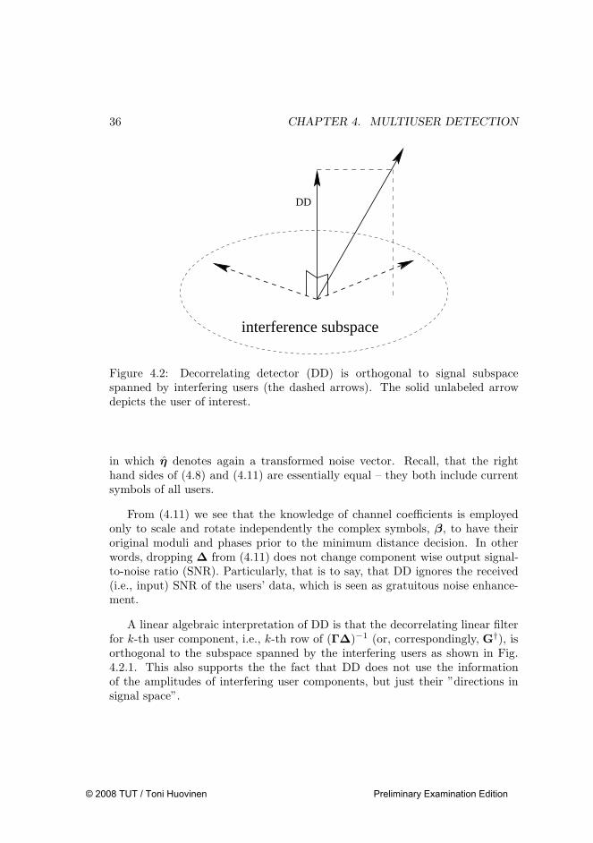
From (4.11) we see that the knowledge of channel coefficients is employedonly to scale and rotate independently the complex symbols, β, to have theiroriginal moduli and phases prior to the minimum distance decision. In otherwords, dropping ∆ from (4.11) does not change component wise output signal-to-noise ratio (SNR). Particularly, that is to say, that DD ignores the received(i.e., input) SNR of the users’ data, which is seen as gratuitous noise enhance-ment.
A linear algebraic interpretation of DD is that the decorrelating linear filterfor k-th user component, i.e., k-th row of (Γ∆)−1 (or, correspondingly, G†), isorthogonal to the subspace spanned by the interfering users as shown in Fig.4.2.1. This also supports the the fact that DD does not use the informationof the amplitudes of interfering user components, but just their ”directions insignal space”.
As discussed in the previous section, the decorrelating detector does not actuallyexploit the knowledge of users’ received amplitudes and noise level and, for thisreason, sufferers from performance degradation especially in low SNR scenarios.In this section, we explore how the performance of linear multiuser detectioncan be improved if we use that knowledge. The improvement must exist, sinceeven conventional single-user detection outperforms decorrelating detector whenSNR is sufficiently low [112].
A key to the performance improvement is the linear minimum mean squareerror (LMMSE) detection that maximizes the MSE function,
MSE(M) := E (‖b− MHr‖2)
(4.12)
with respect to the matrix variable M ∈ C2C×3K [112]. The matrix that maxi-mizes (4.12) is [61]
M0 = Cr−1G, (4.13)
in which Cr = E (rrH)
is covariance matrix of the received data (cf. LMMSEvector (3.30) in Section 3.4). Decision statistics of LMMSE detection is
yLMMSE := MH0 r. (4.14)
An important property of the LMMSE transformation (4.13), which we al-ready discussed also in Section 3.4, is that it maximizes the linear signal-to-interference-and-noise ratio (SINR). Or to be more precise, the k-th column ofM0, m0 = Cr
−1gk, maximizes the linear SINR, i.e., SINR wrt. the symbol bk
at the output yw = wHr among all linear filters w ∈ C2C . Recall that wegave the rigorous definition of SINR in (3.25) in Section 3.4. In other words,the components of the LMMSE output, yLMMSE, has maximum linear SINRwrt. the corresponding components of b. Of course, SINR is scale-invariantand, consequently, scaling columns of the matrix G in (4.13) does not changecomponent-wise SINR. However, the covariance matrix Cr in (4.13) includesimplicitly the information of users’ received amplitudes and noise level mak-ing the LMMSE detection more sophisticated compared to decorrelating one.We can think that LMMSE detection is optimal linear trade-off between thecomplete mitigation of multiaccess interference and the best noise reduction.This is strictly true only in the SINR sense. In the bit-error-probability sense,the optimality (among linear receivers) is not exactly attained by maximizingSINR unless the component-wise total interference after linear transformation
is Gaussian [112]. In practise, however, the interference is approximately Gaus-sian thanks to the well known central limit theorem provided that number ofactive users is relatively high.
4.3 Nonlinear suboptimum MUD
The decorrelating detection and LMMSE detection described in the previoussection are the most important examples of linear MUD methods. In this sec-tion, we consider non-linear MUD methods, that is, the methods that can notbe presented as a linear transformation of received data (followed by minimum-distance decision). Typically such methods have the interference subtractivenature meaning that the multiaccess interference or at least some portion of itis first estimated and then subtracted from received data prior to demodulationof the user’s symbols.
4.3.1 Successive interference cancellation (SIC)
Successive interference cancellation (SIC) is a non-linear suboptimum multiuserdetection method. The basic idea in SIC is to detect the symbols of interferingusers one by one. After detecting a symbol of one user the wave form carry-ing the symbol is recreated and subtracted from the remaining signal beforedetecting the next user’s symbol [112]. Recreation of the wave form (as wellas detection of symbols) is possible only if the spreading codes of all interfer-ing users are known by receiver. In addition, to be able to recreate the waveforms of the users, the delays and path gains of each user should have beenestimated [43].
The main principle of SIC detector is shown in Fig. 4.3. The signal rk(t), k =1, 2, . . . , K, which is used as received signal for detection of the k-th user cannow be formulated as [43, 112]
rk(t) =
r(t) , when k = 1 and
r(t) −∑k−1
l=1
∑Mm=1 albl[m]ξl(t − mT − τl) , otherwise,
(4.15)
where r(t) is the original received signal and ξl(·), al, τl and bl[m] are thespreading code, path gain coefficient, delay and estimate of the m-th symbol ofthe l-th user, respectively. Note that the symbols from the first to the (k−1)-thuser have already been estimated when the signal rk(t) is about to be generated.
Typically, the conventional single-user matched filter detector is used to obtainthe symbol estimates [112].
If the decision of user’s symbol is correct, the multiaccess interference (and ofcourse total interference also) decreases during every substraction. If the detec-tion is incorrect, subtraction actually enhances the interference. Consequently,the order in which users are demodulated and subtracted affects the reliability ofSIC. Thus, the user which is the most likely to be detected correctly or, in otherwords, has the best received SINR, should be processed first and so on [43,112].One way to proceed is use the decreasing order of received power estimates [43].This method is popular since it is simple to implement. However, it does nottake into account cross-correlations between users spreading codes. A betterway to order the user is to use, e.g., MF output of the user [112].
The performance of SIC is analyzed in [87,112]. SIC was found to outperformthe conventional detectors clearly. SIC increases both the system performancein a multipath fading environment and the robustness against near-far effect.Thus, the capacity of the system can also be increased with a SIC based receiver[87]. Compared to optimum MUD, SIC does not give quite as good performanceimprovement [112]. On the other hand, the number of cancellations made in SICis (at most) K − 1, where K is the number of users, and every cancellation hasa constant computational complexity in the number of user. So, the complexityof SIC is (almost) linear in the number of users [112] (the only non-linear partin SIC is ordering the users) whereas it is exponential for the optimum MUD.
4.3.2 Parallel interference cancellation (PIC)
Parallel interference cancellation (PIC) is another non-linear suboptimum mul-tiuser receiver structure. Like the successive interference cancellation, the PICis also based on the idea of estimating and subtracting the multiaccess interfer-
ence (MAI) from the received signal before processing it. Though, interferencecancellations are accomplished in parallel manner. We consider here only thedata detection methods using PIC, but the PIC ideology is also used for channelestimation and delay tracking (see, e.g., [67, 69]).
In the basic PIC [39,69], the received multiuser signal is first passed throughthe bank of K matched filter, where each filter is matched to spreading code ofone user. Then the MAI affecting the demodulation of each user is estimated andsubtracted from the matched filter outputs. In order to estimate the MAI, thechannel parameters should naturally be first estimated. Finally, the minimumdistance decision is used to obtain the hard estimates of users’ symbols.
The multistage algorithm by Varanasi and Aazhang is one of the PIC basedmethods for data detection [108]. The detection of users’ symbols is done inP stages (see Fig. 4.4). Before making the p-th, p = 1, 2, . . . , P , stage decisionof user’s symbol the MAI is estimated and subtracted from the received signal.The MAI estimation in the p-th stage is made using the symbol estimates ofthe (p − 1)-th stage. Hence, the p-th stage decision statistics of the k-th user’sthe m-th symbol can be written as [108]
ypk[m] = yk[m] − Υp−1
k [m] (4.16)
where yk[m] is the MF output and Υp−1k [m] is the (p − 1)-th state’s estimate
of MAI affecting on the m-th symbol of the k-th user. The p-th stage’s MAIestimate is defined more exactly as
Υpk[m] :=
K∑
l=k+1
albpl [m − 1]kl +
∑
l 6=k
albpl [m]kl +
K−1∑
l=1
albpl [m + 1]
kl, (4.17)
where al denotes a channel coefficient of the l-th user and bpl [m] an p-th stage’s
symbol estimate of l-th user’s m-th symbol. kl, kl and kl
are the asynchronouscorrelations between users’ spreading codes defined rigorously in Section 2.2.Recall, that the MAI affecting on yk[m] is characterized as
Υk[m] =
K∑
l=k+1
albl[m − 1] kl +∑
l 6=k
albl[m] kl +
k−1∑
l=1
albl[m + 1] kl
. (4.18)
Thus, the MAI is totally cancelled in the p-th stage if the symbol estimates ofthe (p−1)-th stage are correct (assuming ideal channel and timing estimations).In the first stage, the MAI estimation can be done using the symbol estimates
Figure 4.4: The multistage PIC detector. A bank of K matched filters which isfollowed by K P -stage processors. Each processor estimates the MAI affectingon the symbols of the corresponding user in each stage. The MAI estimated onthe (p − 1)-th stage is subtracted from the MF output before the estimation ofthe p-th stage.
Figure 4.5: Needed symbol estimates from each stage to obtain the estimates ofthe m-th symbols in the 2-stage PIC detector.
obtained directly from matched filter outputs. The symbol estimates obtainedin the last (P -th) stage is considered as the final decisions.
As seen in (4.17), the three successive symbol estimates from previous stagesfor each user is needed to obtain one, say m-th, symbol estimates for each userin current stage. Recursively, three symbol estimates from the stage (P −1), fivesymbol estimates from the stage (P −2), . . . and finally 1+2P symbol estimatesfrom the initial stage is needed to obtain the final (the P -th stage’s) estimatesof the m-th symbols [67, 108]. Figure 4.5 shows an example of the neededsymbol estimates in case of the 2-stage detector. Consequently, all needed sym-bol estimates should be stored until they are not needed anymore [108] and,hence, implementations should contain relatively large amount of memory. Inaddition, roughly half of the previous stages’ symbol estimates needed in thecurrent stage, are estimates of the subsequent symbols with respect to the sym-bol being processed. As a result, an additional processing delay is involved inmultistage algorithm [108].
The performance of the multistage PIC detector is experimented numeri-cally in [108]. A significant performance improvement was found compared tothe conventional single-user detector even with small number of cancellations
stages. Moreover, the improvement was getting even more outstanding whenthe number of stages was getting larger. Also the computational complexityof the multistage algorithm is dealt with in [108] and a conclusion is that thealgorithm is linear with respect to the number of users, i.e., the algorithm hasthe complexity of O(K). This is valid if only one user is detected. Hence, fordetection of all active users (which is usually the case in the uplink receivers),the PIC algorithm has the computational complexity of O(KK) = O(K2).
Some modifications to the basic multistage algorithm have also been done.The improved version of the multistage algorithm is derived by in [25]. Inthe original multistage algorithm, the whole estimated MAI is subtracted inevery stage. In the improved version, on the contrast, only a fraction of theestimated MAI is subtracted in the early stages such that the amount of MAIbeing subtracted is getting larger as the algorithm proceeds. Since the reliabilityof tentative decisions is relatively poor in the beginning of the algorithm andgets better towards the end, the use of gradually increasing weights for the MAIestimates reduces the influence of erroneous tentative decisions. This improvesthe performance of the multistage algorithm.
4.3.3 Comparison of SIC and PIC
The performance of the SIC and basic PIC based detectors is compared in[88]. The main findings are that, first, if all users are received with equalstrength, then the PIC based receiver outperforms the SIC based one. Secondly,in the case of inequal received powers SIC gives better performance than PIC.Recall that in the SIC method the users are first ordered such that in everysuccessive cancellation the user cancelled is the strongest one of the remainingusers. However, if all received users have nearly equal strength, this orderingcannot be done properly. This explains why SIC can provide relatively betterperformance if received powers are not equal. Thus, the SIC method was foundto resist the near-far problem more than PIC.
Nevertheless, only 1- and 2-stage PIC was considered in the experimentsin [88]. The multistage PIC also with more than two cancellation stages isconsidered as a reference method in [P1–P8]. An interesting finding is thatthe performance of the PIC receiver with more than three cancellation stagesseem to be dramatically different from the performance of the PIC receiverwith only one or two cancellation stages in the system with a severe near-far problem. In our experiments, the performance of the PIC receivers withmore than three cancellation stages was actually getting better while near-farproblem was getting worse. Moreover, the PIC receivers with more than three
cancellation stages outperform the SIC receiver clearly also in the cases of a badnear-far problem.
We shall also compare the complexity of SIC and PIC shortly. Like seenin Sections 4.3.1 and 4.3.2 the SIC method has linear and the multistage PICmethod quadratic computational complexity in the number of users. However,the processing delay is also linear in the number of users in the successive can-cellation [112]. Whereas, the multistage PIC can be implemented such that ithas a constant processing delay in the number of users and linear in the numberof cancellation stages [108]. Thus, if the number of stages used in the PIC isrelatively small and the number of users is relatively large, the PIC receiver canprovide shorter processing delay than the SIC receivers.
4.4 Blind MUD
As “blindness” has been a vogue concept in the signal processing society dur-ing the past years, the word ‘blind’ has been attached to names of numerousand quite different signal processing methods and algorithms. Accordingly, ameaning of the word varies from a context to another. Also this thesis treatswith two distinct concepts that are referred to blind in the literature, but wherethe notion has different meaning. In Chapter 3, we already discussed the blindsource separation (BSS), i.e., the signal processing concept aiming to recoversource variables or signals from their linear mixtures. One could say that BSSmethods are blind in the strict sense, since they are not allowed to use basi-cally any explicit knowledge of the sources (except maybe the number of them)and the mixing transformation. These methods rely only on some very generalidentifiability assumptions like bijectivity of the mixing transformation and, forexample, statistical independence of the sources.
The other concept referred as blind and considered here, is blind multiuserdetection [111, 112, 114, 115]. When detecting a DS-CDMA user, blind MUDreceivers assume the same knowledge as the conventional single-user receiver,that is, the spreading code and channel state information (including timing) ofthe user of interest only. In addition, they implicitly assume an existence of MAIfrom other users of the system and try to learn or mitigate it in the blind manner.Thus in this case, the notion of blindness is somewhat looser than in the formercase – from BSS’s point of view, blind MUD receivers use partial knowledge ofmixing transformations explicitly. The following subsection (Subsection 4.4.1)consider blind counterparts of the suboptimum MUD methods discussed in theprevious sections. Also BSS/ICA assisted MUD receiver structures (Subsection
4.4.2) can be seen as blind MUD methods, although some of them (in particular,receiver structures proposed in [P1–P8]) consist of two separate stages: a fullyblind separation stage and an non-blind identification stage following after theseparation. This type of structure is often referred as ‘semi-blind’.
In rest of this section, we use again the stochastic data model,
r = Gb + η, (4.19)
that we introduced in Section 3.2 (Eq. (3.11)). Recall also, that we have assumedthe additive noise term to have the covariance matrix E (ηηH
)= σ2I with σ2
being the noise variance.
4.4.1 Subspace decorrelating and LMMSE detection
The purpose of subspace detection methods [112,115] is to achieve a blind MUDreceiver in the sense described above. Thus, we assume here that receiver knowsonly one column of the matrix G in (4.19), the column corresponding to the(“middle” part) of the user of interest. That column vector – let us assume itis the k-th column and denote it by gk – consist, essentially, of the spreadingcode vector of the user with correct timing. The other columns of G, we assumeas unknown. In addition, we assume the noise variance σ2 to be known by thereceiver.
When deriving a blind variant of decorrelating detector (DD), the objectiveis to find the k-th row vector of the pseudo inverse G† by observing received datar and using the vector gk. This is equal to finding a vector orthogonal to thesignal subspace spanned by multiaccess interferers, that is, the other users thanthe one of interest. The row vector in question is found (blindly) by inspectingthe the covariance matrix of received data [112]. We can write the covariancematrix as
Cr := E[rrH ] = GGH + σ2I. (4.20)
Now, since the covariance matrix is hermitian and positive definite, it has aneigendecomposition of the form Cr = EΛEH with an unitary matrix E anda positive definite diagonal matrix Λ [104]. Consequently, we can write thecovariance matrix also as
Finally, we obtain the k-th row vector of G† from the most right hand side of(4.23) as
g†k := gH
k E(Λ− σ2I)−1EH . (4.24)
Since the covariance Cr can be learnt by observing received data, gk is suf-ficient information to construct the DD receiver of the desired user in (4.24)assuming that noise power is known or estimated. Especially, explicit informa-tion of MAI is not needed, thus, this variant of DD is a blind MUD method inthe sense described above. In practise, to be able to learn the covariance Cr
or its eigendecomposition adequately, receiver must observe received data fromlonger time period than just over the one symbol, which is enough in non-blindDD reception. In other words, the receiver is able to learn the signal subspace inwhich MAI lies by observing received data over a longer period period of time.
Similarly, we can construct subspace variant of LMMSE receiver straightfor-wardly from (4.13) as
mk = EΛ−1EHgk. (4.25)
This is, thus, the k-th column of LMMSE matrix represented in terms of signalsubspace formalism. Also other blind adaptive MUD algorithms with theoreticalperformance equal to LMMSE receiver, are proposed in the literature [34, 72,73, 112]. These are based on minimizing output energy of “canonical” matchedfilter output, that is essentially, minimizing
MOE(v) := E ((gk + v)Hr)2
, (4.26)
with respect to v ∈ C and subject to orthogonality constraint vHgk = 0. Itcan be shown that, the canonical form gk + v′ maximizes LMMSE for mini-mum point of (4.26) denoted by v′ [73]. This minimum output energy (MOE)formalism enables the adaptive gradient descent algorithms that need only thesame information than the conventional single-user detector.
Also a concept of blind multistage interference cancellation and blind suc-cessive cancellation are proposed in [99] and [100], respectively.
4.4.2 ICA assisted MUD
Recall from Section 3.2, that DS-CDMA model (4.19) is actually the noisyICA model. Therefore, extracting source components from received data, r,with ICA, is basically what is required of multiuser detector. Nevertheless,
due to ICA’s phase and permutation unambiguity, separation alone is not quiteenough for detection of users’ data – source components need to be identifiedafter separation or, alternatively, the unambiguities must be removed before it.This can be done if the receiver knows at least the spreading code(s) of theuser(s) of interest. In principle, ICA assisted receivers considered here use thesame information as needed in blind MUD methods, i.e., the column(s) of thematrix G corresponding to the desired user(s).
At this point, it is good time to set the question: “Why in earth wantssomeone use some considerably weighty blind statistical ICA algorithm if weanyway must know essentially all the information the algorithm can give us?”Fortunately enough, the answer is simply: in practice, the receiver does notknow the needed columns of G exactly. It only knows estimates of them thatare affected by channel and timing estimation errors. However, ICA algorithms,as being fully blind, are not affected by these errors. The ambiguity removaltask after the actual ICA separation, in turn, is not very sensitive to theseerrors [P1–P8]. Thus, the effect of erroneous knowledge of the matrix G can becompensated using ICA. In the following, we assume that the receiver knowsonly erroneous estimate of G or its k-th column and denote them by G and gk,respectively.
From performance point of view, ICA assisted MUD receivers are, concep-tually, closely related to decorrelating and LMMSE receivers. Namely the ob-jective of ICA algorithms is, essentially, to find (pseudo-)inverse of the matrixG or at least one row of it (cf. one-unit algorithms). In other words, the algo-rithms try to find the decorrelating detectors of the active users. Under noisymodel, this is strictly true only if, so-called, noisy ICA algorithms (see Section3.1.2) is used. However, as described in Section 3.4, the basic (noise-free) ICAalgorithms that include pre-whitening stage, e.g., the FastICA algorithm, tendto estimated the LMMSE matrix related to the model in hand. Hence, usingthese algorithms resembles basically LMMSE reception.
One of the first BSS/ICA assisted DS-CDMA MUD receiver structure wasproposed in [98]. Starting from the model (4.19), the proposed receiver simplyuses the one-unit FastICA algorithm to separate the desired user from multiac-cess interference. However, the one-unit FastICA applied such as, can convergeto any user component in the system due to ICA’s permutation indeterminacy.To circumvent this problem, that is, to make FastICA to converge to the desireduser, the receiver uses the the vector gk, or strictly speaking, the correspondingLMMSE vector mk := EΛ−1EH gk (cf. (4.25)), to initialize FastICA. The ideais to start FastICA algorithm from initial point close enough to the desired (andunknown) target point and by this way guarantee the converge to the right ba-
sis vector. Nevertheless, sometimes the FastICA algorithm may converge to awrong basis vector although the initial value is selected wisely. In these cases,the conventional detection provides likely a better performance than ICA. Forthis reason the the receiver includes also “a branch switching” between the con-ventional and ICA assisted detection methods as a final step of the reception.The branch switching is performed by measuring the difference between initialand final point(s) (or vector(s)) of FastICA. If the difference is small enough, theICA assisted branch is selected. Otherwise, the FastICA algorithm has the mostlikely run away from neighborhood of the desired basis vector and converged toanother one, thus, output of conventional receiver is used.
In Publications [P1,P2], we derived and analyzed a semi-blind receiver struc-ture for the DS-CDMA uplink. In uplink receivers (e.g., in base stations ofcellular network), all the active users need to be detected. Hence, the receiveruses the symmetric FastICA algorithm to separate all the active users from oneanother. The receiver, nevertheless, is not totally blind, since users are iden-tified using the pre-knowledge of the users, that is, the pre-estimated matrixG, after the separation. When identifying the k-th user, the receiver evaluatecorrelations between gk, and ICA’s basis vectors, say wk′ , that are estimatedby FastICA. That is to say,
θ(k, k′) =gkw
Hk′
||gk||||wk′ ||(4.27)
is computed for each k′. Finally, the source which corresponds to the best cor-relation is chosen to be that user’s data. Furthermore, the phase of complexnumber θ(k, k′) in (4.27) equals to arbitrary and unknown phase shift producedby ICA. This makes it possible to correct ICA’s phase ambiguity. This simplestidea of using ICA to separate DS-CDMA users from each other has been rein-vented several times in literature [28,30,31,102,103] since the author introducedit first time in his M.Sc. thesis [44].
Sometimes FastICA fails to recover some of the data components satisfy-ingly due to noise and other imperfections in the model. Poorly estimated datacomponents impair the performance of reception, especially when the numberof users is high. However, if an estimated source signal is of low quality, the cor-responding column of estimated mixing matrix is usually defective, also. Thismakes it possible to recognize poorly estimated users. To elude this problem,we introduced an idea of adapting the concept of successive interference can-cellation (SIC) to the ICA assisted receiver in Publication [P3]. The principleof this successive ICA receiver is rather straightforward. First, a correlation
threshold, say θ1, is set to indicate proper detection. This is needed becausesubtraction of erroneously detected signal will actually enhance interference.Thus, after the symmetric FastICA separation, only the signal corresponding tothe user k with θ(k, k′) > θ1 for some k′ is subtracted from the receiver signal.After subtraction of all such users’ signals, a new ICA separation is performedfor the interference-subtracted signal. The order of ICA model decreases insubtraction, which help ICA to recover the remaining users. The procedure isrepeated successively until all users are detected. The successive ICA receiveris illustrated in Fig. 4.6.
An another recent study has also found blind source separation techniquesto be beneficial in interference subtractive receivers [105]. In that study aniterative least squares technique for digital signal separation was enhanced by aninterference cancellation stages, a procedure similar to conventional successive orparallel interference cancellation schemes. Namely, the method takes advantageof an alternating estimation of the mixing matrix and user symbol streams inuntil converged, while employing an interference cancelling stages during thesymbol streams’ estimation.
Recall from Chapter 3, that the major drawback for standard ICA methodsis the oversaturated model where the number of source signals is greater thanthe number of observations made in which case standard ICA model does nothold anymore. And further recall, that, from the single antenna DS-CDMAreception point of view, the data model become oversaturated if the numberof users is greater than two third of processing gain (K > 2
3C), assuming pro-cessing window size of two symbols. Hence, the number of users in the systemmust be rather low to make standard ICA applicable. In Publications [P4–P6],we showed that this “more sources than sensors”-problem can be somewhatcircumvented in the successive-type ICA receiver, in particular, if received pow-ers of the users are inequal. This is mainly based on the PCA pre-whiteningtask of FastICA, which is originally intended to make the remaining separationprocedure simpler. However, since relative magnitudes of the eigenvalues are,in practice, directly proportional to the strengths of independent componentsthe whitening by PCA tends to prefer the strong components, and some weakcomponents might be lost [78]. In general, this is an undesirable phenomenon,since ICA algorithms should not be sensitive to the differences in componentstrengths. Nevertheless, the successive ICA receiver structure benefits of thisphenomenon. Namely, as PCA processing prefers relatively strong users, theseusers are detected more likely after ICA separation. On the other hand, in-terference subtractions are performed for original, unwhitened data, which isnot affected by PCA. Hence, originally relatively weak users are intact after
Figure 4.6: Successive ICA assisted receiver structure. ri(t) and ri are a receiveddata signal and a received data vector after the (i−1)-th IC round, respectively(r1(t) = r(t) and r1 = r). Vector yi
ICA is source components by FastICAseparation. Number of components in that vector decreases in each IC round.Soft and hard decisions of users’ symbols are denoted by bi and bi, respectively.Υi(t) denotes interference due to users detected in i-th round.
the subtractions. How these users can be detected after following ICA separa-tions depends on their relative strengths and number. This all is to say, thatin a sense, PCA preprocessing hides the weak users in early separation stageswhereas subtractions reveals them again in the later ones. Therefore, the suc-cessive ICA receiver structure provides the best performance gain when numberof users having (nearly) equal received powers is small enough.
One should recognize the fact that, conventionally, in interference subtrac-tive receivers, like in SIC, a very precise channel state information is needed inthe interference subtraction to prevent interference enhancement. This is whyalso accurate code timing acquisition and tracking is of great importance. How-ever, an important property of ICA assisted receivers is its inherent capabilityto cope with erroneous parameter estimates. Roughly speaking, the estimateof interference by ICA implicitly includes also the timing information of theuser signals, thus giving a possibility to refine preliminary delay estimates be-fore re-generation of interfering signals and its substraction. This kind of delayestimate refinement is not inherently possible in conventional interference sub-tractive receivers, but additional delay tracking circuitry is needed. We proposedin Publications [P6,P8] a modification of successive ICA receiver which is, inpractice, immune to delay estimation errors. The modification constitutes of atwo-step delay tracker within ICA processing where a coarse pre-tracking helpsthe identification procedure during ICA and a finer post-tracking improves theinterference re-generation, and hence, enables more effective interference can-cellation. It is of primary importance to stress out, that all timing refinementsare done after the ICA processing. Hence, also the delay tracking proceduretakes advantage of interference suppression due to ICA separation.
The above mentioned ICA assisted MUD-receivers are based on stochasticsingle-antenna DS-CDMA model directly. Also receiver structures using ICAthat are based on multi-antenna model is proposed in literature. For exam-ple, [86] introduces such a structure. More in detail, the proposed method max-imizes the multiuser kurtosis among linear transformations of received data. Another example of multi-antenna methods is proposed recently in [79]. It uses atensorial ICA method.
4.4.3 Discussion on complexity of ICA assisted receivers
Considering practical implementation of any receiver structure, the computa-tional complexity of the structure in hand is, naturally, one of the first attributestaken under inspection. However, the most of ICA algorithms – including Fas-tICA – are iterative statistical optimization algorithm, where a needed number
of iterations before convergence is random in its nature. For this reason, derivingoverall complexity of ICA algorithms is difficult. In [44], the author concludesthat the complexity of the simple (non-successive) ICA receiver [P1,P2], mea-sured as needed “multiply and add”-operations, is O(K2M)+O(CK2) in whichC, K and M (M >> C, K) denote the length of spreading code, number ofusers and number of symbols (per user) in one received data block, respectively.The derivation of this result is also included for a easy reference in Appendix B.However, this simple analysis does not take into account how a needed numberof FastICA iterations depends on parameters C, K and M , but rather considersthe number of iterations only as a constant.
The most natural way to affect the convergence speed of an ICA algorithm or,in other words, keep the needed number of iterations in moderate level, is to usethe known and pre-estimated system parameters when initializing the algorithm.Considering the FastICA algorithm, for instance, and assuming that we initializeit with the “whitened” LMMSE matrix related to G, we actually start theiterations from some close neighborhood of the actual ICA solution providedthat G ≈ G. Hence, we can expect to obtain a convergence after a very smallnumber of iterations in that case. This is also demonstrated by new results inAppendix A. Moreover, using information included in G to wise initialization is,in general, a sensible and simple way to embed the approximative pre-knowledgeof the system in ICA separation stage.
The subtractive ICA assisted structures [P3–P8], in turn, consists of (a few)successive repetitions of the symmetric FastICA separation stage. In addition,the fist separation is computationally the most demanding, since a dimensionof ICA model (actually, the parameter K) decreases after each stage. Conse-quently, the complexity the successive structures is basically of the same orderthan the complexity of the simple ICA receiver.
In the previous chapter we discussed several methods of mitigating an inter-nal MAI due to non-ideal cross-correlations between spreading sequences in aDS-CDMA system. Naturally, also some external sources can interfere the DS-CDMA reception. Here, we mean by an external interference signal, basically,any non-Gaussian signal component other than MAI. These signals can be, e.g.,some spurious narrowband signals originated from nearby RF channel or wide-band spread spectrum signals from adjacent cell of a cellular system. Also anintentional jamming is possible, especially, in military systems. In this chapter,we discuss the rejection of external interference shortly. First, we define the ex-ternal interference signal rigorously in Section 5.1. Then, in Section 5.2 we givebrief overview of conventional ideas to fight against narrowband interference.In the end, in Section 5.3, we continue by discussion on an inherent capabilityof the ICA assisted receivers to resist external interference.
5.1 External Interference in Signal Model
We model the external interference signal, say Υext(t), as a continuous wave(possibly pulsed at the symbol level) with an amplitude AΥ ∈ (0,∞), frequencyfΥ ∈ R and phase φΥ ∈ [0, 2π):
during a symbol duration, i.e., χp(t) ≡ χp[m] ∈ 0, 1 for t ∈[(m − 1)T, mT
).
Hence, the interference corresponds to a continuous wave when p = 1 and pulsedwave at the symbol level otherwise.
We obtain a special case of the (5.1) assuming that the frequency, fΥ, islocked to the carrier frequency used in the system. In this case, the externalinterference signal remains constant during one symbol duration also after thedown conversion (assuming that the phase of the signal is constant). Hence, inthis case, we can write the (base-band) interference signal as
Υext(t) = Υext[m], for t ∈[(m − 1)T, mT
), (5.2)
where Υext[m] := χp[m]AΥeıφΥ[m]. In addition, we assume that the phaseφΥ[m] is a sample of an uniformly distributed random variable having values in[0, π). This presentation is assumed also in Publications [P1–P3,P6–P8] and,e.g., in [96, 97].
The received signal has now the form
r(t) = rif(t) + Υext(t + τΥ), (5.3)
where rif(t) is the original external interference-free signal and τΥ ∈ [0, T ) isa formal temporal phase of the interference signal. For sake of simplicity, weassume that τΥ is an integer multiple of chip duration TC .
We can embed the external interference also into the stochastic, matrix alge-braic representation (3.11) defined in Section 3.2. Namely, after chip-matchedfiltering, the m-th received data vector of length 2C becomes
Hence, if we extend the original code matrix, G, with three column vectors 1,1 and 1 and the original symbol vector, Bm, with three interference symbolsΥext[m − 1], Υext[m] and Υext[m − 1], we get the same representation,
r[m] = GBm + η[m], (5.6)
for the data as in interference-free case. Again, we interpret r[m], Bm andη[m], m = 1, . . . , M , as ergodic samples of some underlying random vectors r,b and η that also follows the affine relationship,
r = Gb + η. (5.7)
Thus, the data model with external interference still corresponds to ICA modelwith three additional source components.
5.2 Conventional Narrowband Interference Re-
jection
Several techniques to improve the performance of the spread spectrum systemin the presence of narrowband interference (NBI) have been proposed duringthe past. Recall, that the external interference signal defined in (5.1) and (5.2)corresponds to NBI signal if pulse probability p = 1. An inclusive review ontraditional NBI cancellation methods can be found in [4], [75], [94] and referencestherein. Here we go through the most typical NBI methods briefly in conceptuallevel.
In contrast to an energy of the spread spectrum signal, all energy of narrow-band interference is concentrated to some slender frequency band near a centralfrequency. Consequently, if a spread spectrum signal is interfered by a narrow-band signal and total energies of the signals are somewhat in the same level, thepower density spectrum has a clean peak on the band of the narrowband signal.The typical proposed NBI cancellation methods exploit this spectral feature inone way or the other.
The simplest NBI cancellators use some (adaptive) notch filter whose stopband equals approximately to the band of the interferer. This approach surelyremoves the interference signal almost totally, but in pursuance, causes somedamage to the desired data signal. However, if the attenuated band is verynarrow with respect to the total band width of the spread spectrum signal, thedamage caused might be more tolerable compared to the interfering effects ofthe narrowband signal. More sophisticated NBI cancellation approach proposed,
Figure 5.1: Estimator–subtractor. A narrowband interference cancellator inwhich the interference, Υext(t), is first estimated using either a linear or non-
linear filter. The estimated narrowband interference, Υext(t), is then subtractedfrom received signal before a detection of symbols.
is depicted in Fig. 5.1. The main idea in these cancellators is to estimate thenarrowband signal and then subtract the estimate from the received signal beforethe detection of users. If the estimate subtracted equals exactly to the originalinterference signal, the interference is totally cancelled and no damage is causedto the spread spectrum signal (cf. subtractive MUD methods). Naturally, theperfect interference estimate cannot be obtained, but some estimation error isalways made. The estimation of the interference is based on the fact that thenarrowband signal is well predictable compared to the spread signal which isalmost random in time domain. The NBI estimator can be implemented, forinstance, by linear or non-linear filtering.
Another typical NBI cancellation scheme, which can be considered moresophisticated than simple notch filtering, is frequency domain NBI suppression.The functionality of such a cancellator structure is shown in Fig. 5.2. A receivedsignal is first Fourier-transformed. This reveals the spectral power peak dueto narrowband interference. Now, the peak can be attenuated by cutting offthe power density spectrum from some predetermined power level (see Fig.5.3). This threshold level should be determined such that the power densityof the desired spread spectrum signal stays only just under the level in wholefrequency band. After frequency domain handling, the modified signal is inverse-transformed to time domain before the detection. In principle, the frequencydomain cancellation does not harm the spread spectrum signal at all. On theother hand, the interfering signal is not removed totally. Some portion of theinterference energy always remains after this kind of cancellation procedure.
Figure 5.2: Frequency domain NBI cancellator. The received signal (which con-sists of the spread spectrum signal, r(t), and narrowband interference, Υext(t))is first Fourier-transformed (FT). Then the NBI cancellation is performed in fre-quency domain. Finally before the detection of users in the system, the modifiedsignal is inverse-transformed (IFT).
SS signal
NBI
Cut−off−levell
P
f
Figure 5.3: NBI cancellation in frequency domain. The received signal is pro-cessed in frequency domain by cutting off the parts of the power density spec-trum which exceed some predefined power level. This attenuates the narrow-band interference signal that has its all energy concentrated near one frequency.
If some external interference signals are present in the system, they can be nat-urally assumed to be statistically independent from desired signal components.Consequently, ICA considers them as additional source components and inher-ently tends to separate them as well. Moreover, since ICA is a time-domainmethod, it does not make difference between narrow- and wideband interferers.Understandably, possible interference components can not be identified afterseparation, since known code sequences are not associated with them. Nev-ertheless, identification of undesired interference components is not necessary.Matter of substance is that the desired components, i.e., the components dueto users’ data, are not affected by external interference in ICA assisted receiverstructures. Our results in Publications [P1–P3,P6–P8] show that all the ICAassisted receiver structures proposed in this dissertation cope with external in-terference as such.
Two rather similar receiver structures that are particularly designed for ex-ternal interference suppression in DS-CDMA downlink is proposed in [9, 97].These structures assume an use of antenna array to obtain ICA model and con-sider a transmitted multiuser signal as one source component and the externalinterference signal as other. Notice, that an input of the j-th antenna, say uj,is basically a noisy linear combination of downlink multiuser signal, say rdl(t),and the interference signal, that is,
uj(t) = αjrdl(t) + βjΥext(t) + η(t) (5.8)
with αj , βj ∈ C. The receivers then use ICA to separate the interference signaland the multiuser signal before detection of the desired user’s symbols. Thus,in these receivers ICA is not applied to separate the CDMA users from eachother, i.e., ICA does not reduce multiaccess interference. The detection itself isproposed to be performed using some standard DS-CDMA detector. A selectionof the correct source signal prior to detections is performed either with help ofpilot information assumed to be embedded in the original multiuser signal orusing known information of spreading codes of the desired users. The mainprinciple of such receiver is illustrated in Fig. 5.4.
Figure 5.4: ICA based interference mitigation structure which use an antennaarray of J antennas. rp(t) stands for a pilot signal which is used to select thedesired source component after separation. Here, the conventional single-userdetector (or RAKE) is used for the final DS-CDMA detection. Basically, RAKEcan be replaced with any detection method.
The second part of this dissertation is a compilation of eleven original researchpublications reporting the novel scientific contributions of this dissertation workin detailed manner. We have referred to these publication as [P1–P11] through-out the dissertation. In this chapter, we summarizes the content of the pub-lications briefly (Section 6.1) and describe the author’s contribution in them(Section 6.2).
6.1 Overview of Contents
Publication [P1] introduces the idea of employing BSS/ICA in DS-CDMA mul-tiuser detection. It evaluates the effectiveness of the simple BSS/ICA assistedlinear receiver against conventional non-linear interference cancellation schemes.The systems with and without additional external interference are considered.Numerical experiments indicate a clear performance gain in comparison to SICand roughly the equal performance as PIC with few cancellation stages whenno jamming was present. However, even with a moderate level of additionaljamming, BSS/ICA out-performs both the non-linear schemes. The resultsthus show how the blindness of BSS/ICA, even when used in the simple lin-ear receiver, is valuable in making the uplink reception robust against inten-tional/unintentional out-of-cell interference.
Publication [P2] extends the performance evaluation of the simple linearBSS/ICA receiver in DS-CDMA uplink. Especially, the effects of multipaths,
related channel estimation errors and additional external interference are exam-ined and compared to conventional SIC and P -stage PIC schemes. The paperdemonstrates by numerical experiments that benefits of BSS are emphasizedwhen a state of propagation channel is not known perfectly. Moreover, the re-sults shows how robust BSS/ICA methods are in a fixed multipath scenario.As a matter of fact, the performance of BSS/ICA-receiver is greatly improvedwhen the number of paths grows.
Publication [P3] adapts an ideology of successive interference cancellation tothe BSS/ICA assisted uplink reception. The effectiveness of the new method isevaluated against the existing linear BSS/ICA assisted reception and conven-tional non-linear interference cancellation schemes (SIC and PIC). The systemswith and without additional external interference are considered also in this pa-per. Numerical experiments indicate a clear performance gain in comparison toreference methods. Above all, the successive BSS/ICA method outperforms theconventional schemes clearly also when the basic linear BSS/ICA method barelyoutdo them. All this is achieved even though ICA processing was terminatedwith a very mild condition, resulting in low computational load.
Publication [P4] proposes a modification of the BSS/ICA-SIC–type receiver,which, unlike standard BSS/ICA, is able to operate in highly loaded systems.The paper shows the new receiver’s ability to drastically enhance the number ofusers a system can support, given a certain bit-error-rate requirement, comparedto that of conventional PIC and SIC schemes and linear BSS/ICA-alone receiver.The paper also shows how the proposed scheme relaxes the inherent weakness ofstandard BSS/ICA. Namely, the inadequateness in highly loaded systems due tothe “more sources than observations”-problem, which is somewhat circumventedin the proposed successive ICA receiver.
In Publication [P5], the BSS/ICA-SIC–type receiver structure where theusers’ delays are simultaneously tracked is introduced and evaluated via numer-ical examples. The main finding was that SIC-ideology combined with ICA foroversaturated systems is notably beneficial given that certain key parameterslike users’ delays are tracked simultaneously. This is due to fact that the de-lay tracking is performed after the blind separation, which basically outputsinterference mitigated signals. Consequently, the delay estimates and, espe-cially, the multiaccess interference estimates to be subtracted, are more precise.The example cases assumed m = 2C = 62 observations from the mixture ofn = 3K = 66 → 90 sources. Hence, all examples have more sources thanobservations.
Publication [P6] revisits and analyzes the ideas of the preliminary conferencepapers [P3–P5] in an unified manner and proposes further enhancements. Hence
the paper deals with the advanced BSS/ICA assisted interference cancellationstrategies applied in DS-CDMA uplink receivers. The considered receiver struc-tures combine the main benefits of pure BSS/ICA and SIC methods: (i) inherentmitigation of various types of interference sources by BSS/ICA, (ii) robustnessagainst parameter estimation errors due to BSS/ICA, (iii) greatly improved in-terference suppression capability due to novel combination of SIC ideology andICA, especially, in the challenging case of highly loaded systems. Numericalexperiments with DS-CDMA uplink data are given to illustrate the achievedgains in user capacity and bit-error-rate performance compared to conventionalSIC and PIC schemes as well as more an advanced LMMSE-PIC receiver andvariants of BSS/ICA techniques alone.
Publications [P7] gives a brief survey of ICA/BSS assisted DS-CDMA meth-ods in the both uplink and downlink reception. In the uplink, the paper presenta single antenna interference cancellation scheme introduced basically in Pub-lications [P3–P5]. For the downlink case, the paper look at an antenna arrayscheme [96, 97], where ICA acts as a pre-filter to conventional detection, sep-arating the information component from the interference component and thusproviding an interference-free signal to conventional receivers.
Publication [P8] considers the BSS/ICA-SIC receivers in a DS-CDMA re-ception with multi-path propagation. Thus this paper is an extension to Publi-cations [P5,P6]. Numerical experiments reveals the robustness of the proposedscheme against the delay estimation errors which are known to be one of theexpected imperfections at the DS-CDMA receivers.
Publications [P9] and [P11] considers the noisy ICA problem generally, thatis, they do not address DS-CDMA detection directly. However, the resultscan be applied when analyzing the performance of the ICA assisted receiverstructures as discussed in Section 3.4. The former publication, [P9], illustratesthat basic ICA designed for noise-free linear models is able to provide essentiallythe best possible output SINR among all linear transformations of received data,in the challenging case of having both additive noise and interference disturbingthe desired signal observation in a multi-antenna receiver context. Thus in effect,the ICA is able to do joint diversity reception and interference cancellation ina blind manner, such that the output SINR is maximized. In particular, theexperiments indicates that one of the most widely applied ICA algorithms, EASIalgorithm, is, in practice, identical with SINR maximizing generalized eigenfilter(M-GEF) in terms of SINR. In theory, EASI can not attain exactly the M-GEF bound when both noise and interference are present, but difference wasnegligible (< 0.1 dB-unit) in all of the experiments. The paper also shows that,in an important special case of single-source system (i.e., one user and additive
noise), the EASI algorithm provides precisely the greatest linear diversity gainblindly, i.e., performs as a blind maximal ratio combiner (MRC).
Publication [P10] gives an example of takeing advantage of the findingsin [P9, P11]. In the paper, a novel DSP method for mitigating the dynamicoffset interference due to RF blocker self-mixing in direct conversion diversityreceivers is proposed. The proposed technique is stemming from modeling thedynamic offset interference as a linear signal mixture model, and then apply-ing ICA on the set of observed signal vectors. Computer simulations are usedto assess the achievable compensation performance, and based on the obtainedresults, the offset interference can be efficiently mitigated using the ICA basedapproach, while also simultaneously obtaining diversity gain against ordinarychannel noise. Based on the simulated interference tolerance, the paper also dis-cusses through an RF dimensioning example, how the ICA based compensatorcan relax the RF filtering requirements for out-of-band blocker signals in prac-tical receiver design, when compared to ordinary MRC processing. The othermain advantage of ICA based method over the other existing techniques is thatthe proposed method in this paper does not need the channel state information,and thus channel estimation can be basically avoided.
Publication [P11] completes the theme of [P9] taking more an analyticalapproach. The paper shows that conceptually the ICA designed for noise-freelinear models is able to solve, blindly and directly, the generalized eigenvalueproblem exactly, i.e., to provide the best possible output SINR among all lineartransformations of observed data. However, ICA algorithms constraining theestimated de-mixing matrix to be orthogonal (or unitary) can not exactly attainthe optimal solution in general, but in a sense they produce an orthogonalizedversion of the solution. In addition, the paper gives the necessary and sufficientcondition under which the stationary point of the EASI algorithm maximizes thelinear output SINR, and also proves that, in the special case of interference-free(that is, noise only) system, the EASI algorithm can attain exactly the greatestdiversity gain blindly, i.e., performs as a blind maximal ratio combiner (MRC).Further numerical results are also given to show that the performance of theEASI algorithm is remarkably close to the optimal (i.e., the maximal outputSINR among all linear transforms of observed data) also in cases in which theabove mentioned theoretical optimality condition is not met.
The author conducted the scientific research work for this thesis mainly at theDepartment (former Institute) of Communications Engineering, Tampere Uni-versity of Technology. That part of the work is reported in [P3–P11]. Thestudies reported in [P1,P2] date back to the time when the author worked atDepartment of Mathematical Information Technology, University of Jyvaskyla.All the work for the thesis has been done under supervision of Prof. TapaniRistaniemi.
The author was the main contributor for the content of [P1–P6, P8, P9,P11]. In all of these publications, the author was the primary developer of thenovel ideas, carried out the theoretical analysis and simulated proposed methodsnumerically. The author also wrote the bulk of the script for [P1–P4,P6,P9,P11].The scripts of [P5,P8] were mainly written by Tapani Ristaniemi. (Recall thatthe author was the main contributor also in these publications in the sensedescribed above.)
In [P7], the author contributed the part dealing with ICA assisted uplink(single-antenna) reception. The rest of the paper, that is, the downlink (multi-antenna) reception related part, was contributed by Karthikesh Raju. In [P10],the author had considerably smaller role. In that paper the author more or lessonly guided the main contributor, Ali Shahed hagh ghadam, in the ICA relatedissues.
In this dissertation, our target was to study possible benefits of using higherorder statistics (HOS) in DS-CDMA multiuser detection (MUD) and interfer-ence cancellation (IC). We carried out this study by developing new non-linearMUD/IC methods which employ HOS based blind source separation (BSS) and,in particular, independent component analysis (ICA) and comparing their per-formance to existing methods. The main emphasis was on the asynchronousuplink reception and, especially, on highly loaded systems. From ICA’s pointof view, the highly loaded system model equals to challenging model with moresources than observation.
The dissertation consists of two parts. The first (current) part gave an intro-duction and background knowledge of the research area to which the topic of thedissertation work belongs and surveyed the existing literature on the area. Thesecond part (which follows after Appendixes and Bibliography) is a compilationof Publications [P1–P11] that reports the novel scientific contributions of thisdissertation work in detailed manner. In this concluding chapter, we summarizethe contribution of the dissertation.
To begin with, we proposed novel ICA assisted successive interference can-cellation (SIC) schemes that obey the fundamental procedures of conventionalSIC. That is to say, (i) the estimation of interference, (ii) re-generation of in-terference and finally (iii) subtraction of the re-generated interference from theoriginal data. What makes the schemes advanced compared to conventionalSIC is the way of estimating the interference using ICA and a sensitive selec-
tion of the interference sources to be subtracted. The proposed receiver struc-tures combine the main benefits of BSS/ICA and conventional SIC methods.First, they are capable to mitigate various types of interference sources thanksto ICA. Consequently, they do not cancel out only multiaccess interference astraditional MUD methods but also external interference sources. Second, theproposed structures are very robust against channel parameter estimation errorsdue to HOS signal processing of BSS/ICA. One should recall that, traditionally,a very precise channel state information is needed in the interference subtractivereceivers (like SIC and PIC) to prevent interference enhancement. This is whyaccurate code acquisition and tracking has been of great importance in thesereceivers. However, an important property of BSS/ICA is its inherent capabil-ity to cope with erroneous timing estimates. We exploited this feature in theproposed receiver structures, to refine tentative timing estimates after the ICAprocessing before interference re-generation and substraction such that also thetiming refinement procedure takes advantage of interference suppression due toblind ICA separation. Consequently, we were able to relax the requirement ofextremely precise code tracking. This kind of relaxation is not inherently pos-sible in traditional interference subtractive receivers. The third benefit of theproposed receiver structures is their good performance in highly loaded systemdue to novel combination of SIC ideology and ICA. Notice, that this can also beseen as a way to somewhat circumvent the “more sources than sensors” -problemof BSS/ICA.
Noisy models have been an another challenge in BSS/ICA area. In mostof practical applications, nevertheless, the presence of an additive backgroundnoise can not be neglected. Especially in telecommunications, some level ofGaussian noise is always interfering the reception. For this reason, we consideredalso the noisy ICA problem. We showed that conceptually many basic ICAalgorithms designed for noise-free ICA models, can actually provide the bestlinear source separation solution possible in terms of input-output SINR gain.This seems not to be well-understood in the literature earlier. From CDMAreception perspective, this founding means that the performance of BSS/ICAassisted reception is indeed exceedingly competitive against any suboptimumMUD detector.
Finally, we conclude that HOS signal processing makes it possible to exploit“hidden” statistical features of information carrying signals in a way which is notpossible with traditional second-order (SO) methods. For example, in spreadspectrum communications, natural statistical independency between narrow-band data streams transmitted by different users is lost in wideband domaindue to nonideal auto- and cross-correlation properties of spreading sequences.
This results in unavoidable performance lost in conventional SO de-spreadingand detection. HOS assisted methods can, however, employ the original inde-pendency and avoid performance degradation due to multiple access and, aswell, external interference.
In the following “last-minute” numerical experiments, the successive ICA re-ceiver (ICA-SIC) with the wise FastICA initialization is evaluated numericallyagainst an advanced LMMSE and LMMSE-PIC receivers [68]. We initialize Fas-
Cz = I is the covariance matrix of whitened data, V is a whitening matrixand G is an estimated code matrix which differ from the exact code matrix dueto erroneous delay or timing estimation. With this initialization, we actuallystart the FastICA iterations from some close neighborhood of the actual ICAsolution, that is, the exact whitened LMMSE matrix (see Section 3.4), pro-
vided that G ≈ G. Hence, we can expect to obtain a convergence after a verysmall number of iterations. Further, as discussed in [P11] and Section 3.4, anyICA algorithm that performs orthogonalization of the basis vectors can not con-verge exactly to LMMSE solution under noisy model. The original purpose ofthis orthogonalization is to prevent multiple ICA units to converge to the sameICA basis vector. We presume that, after the wise initialization of FastICAalgorithm, the starting point of iterations is such close to point of convergencethat the orthogonality constraint is not needed any more. Thus, we modify theoriginal FastICA algorithm slightly by simply removing the orthogonalizationin order to provide a possibility of the exact convergence to LMMSE solution.Consequently, we expect clear performance gains compared to results in our
earlier ICA-SIC related publications [P3–P8].The simulated system model is asynchronous DS-CDMA model (see Eq.
(2.8) in Section 2.1) with K = 30 users. The users are assumed to be in twoequal sized service classes, which is modeled as a power difference of 10 dBbetween the two user groups. Inside both groups all the users are assigned thesame power. Each user is supposed to sent data blocks of M = 5000 QPSKsymbols. Symbols are spread using Gold codes of length C = 31. In ICA-SIC,value ρ = 0.9 is used for the identification threshold. All results are based onaverage bit error rates (BER) over 1000 independent repetitions. BER valuesare computed with respect to all K users. For estimated LMMSE methods,we have used also the estimated LMMSE matrix instead of the exact one. Inaddition, we have plotted performance of exact LMMSE methods in some figuresbelow.
Fig. A.1 shows performance of the ICA-SIC receiver as a function of numberof iterations in FastICA. The results indicate relatively short convergence time.The best input-output performance gain of the ICA-SIC is obtained, essentially,after 10–25 FastICA iterations depending on SNR level. Comparing this to ourearlier results in which we initialized FastICA randomly, the required conver-gence time has degraded even to one tenth. E.g., in [P6], FastICA converged toadequate performance level only after 110 iterations in extremely highly loadedsystem, i.e., with K = 30 and C = 31.
Figs. A.2 and A.3 compare the ICA-SIC receiver to LMMSE and LMMSE-PIC receivers under erroneous timing estimation. The figures shows clear per-formance gain of ICA-SIC. Most interestingly, ICA-SIC provides better perfor-mance also with perfect timing knowledge (that is, with zero error variance) inFig. A.2. In our earlier results, both LMMSE and LMMSE-PIC outperformedICA-SIC in that case. This performance improvement on the earlier results canbe explained by relaxation of orthogonalization-step of the FastICA algorithm.Hence, the new results support the theoretical founding of [P9,P11] (see alsodiscussion in Section 3.4) that ICA is able to provide the best input-outputSINR gain in noisy model.
Figure A.1: BERs as a function of number of FastICA iterations. FastICA isinitialized with estimated LMMSE matrix. Users’ estimated delays are assumedto have an error δk with variance σδ
2 (unit of error corresponds to one chipduration). SNRs are fixed to 10 dB (top) and 15 dB (bottom).
Figure A.2: BERs as a function of number of variance of delay estimation error.FastICA is initialized with estimated LMMSE matrix. SNR is fixed to 10 dB.
Figure A.3: BERs as a function of number of received SNR. FastICA is initial-ized with estimated LMMSE matrix. Users’ estimated delays are assumed tohave an error δk with variance σδ
2 = 0.025 (unit of error corresponds to onechip duration).
This appendix is substantially direct citation of M.Sc. thesis of the author [44,Section 6.3.2]. The remark on oversaturated data at an end of the appendix, isadded to this PhD dissertation.
Next, we derive the computational complexity of a receiver structure whichuses the symmetric FastICA algorithm. Particularly, the needed number of“multiply and add”-operations is considered. The following derivation does nottake needed number of iterations into account. The complexity of the receiverstructure using the one-unit FastICA algorithm is discussed in [98]. Here, we useconclusions given in that paper to the extent that the symmetric and one-unitalgorithm conjoin.
As previously, C, K and M denote the length of spreading codes, numberof users and number of symbols (per user) in one received data block, respec-tively. Note, that now M >> C > K. The both FastICA algorithms consistpartly of preprocessing tasks, namely the dimension reduction and whitening.Typical eigenvalue based methods for dimension reduction have the complexityof O(C3), which reduces to O(C2K) if only K eigenvalue is needed like in thisapplication [98]. The whitening, for one, can be performed with the complexityof O(CK), when it is assumed that K < C [98].
For the complexity analysis of symmetric FastICA iterations themselves, wecannot directly apply the complexity obtained in [98]. Anyway, the complexity
in the one-unit case is O(KM) per iteration. To estimate all components simul-taneously, the one-unit iteration is, basically, repeated for all components. Thisraises the complexity to O(K2M). In addition, the tentative estimate vectorsshould be made orthogonal between each iteration. Applying the Gram–Schmidtorthogonalization algorithm (GS), for instance, has the well-known complexityof O(CK2) [38]. Thus with GS, the complexity of one FastICA iteration isO(K2M) + O(CK2).
The selection of the right source components should also taken into accounthere. Recall, that the selection is based on correlations
θki =< gk|gi >
||gk|| ||gi||∈ C, (B.1)
where gk and gi are essentially 2C-vectors. Hence, computing one correlationhas the complexity of O(C). Further, 3(K + 1) correlations is computed foreach K users. Thus on the whole, the complexity of computing correlations isO(K2C).
Altogether, given that M >> C > K, the complexity of the Pure ICAreceiver is O(CK2) + O(K2M).
Remark. If we assume oversaturated data (K > C), which is more practical inDS-CDMA systems as seen in this PhD dissertation, only the complexity of thewhitening process changes from O(CK) to O(C2) in above analysis. Further,since C2 < CK2 (in this case), the final conclusion of the complexity stayssame.
[1] S. Amari. Advances in Neural Information Processing Systems 9, chapterNeural learning in structured parameter spaces — natural riemanniangradient, pages 127–133. The MIT Press, Cambridge, MA, USA, 1997.
[2] S. Amari, A. Cichocki, and H.H. Yang. Advances in Neural InformationProcessing Systems 8, chapter A new learning algorithm for blind sourceseparation, pages 757–763. The MIT Press, Cambridge, MA, USA, 1996.
[3] S.-I. Amari. Natural gradient learning for over- and under-complete basesin ICA. Neural Computation, 11(8):1875–1883, 1999.
[4] F. Amoroso and R. A. Monzingo. Techniques to improve anti-jam perfor-mance of spread spectrum systems. In Proc. IEEE ISSSTA1996, pages636–646, 1996.
[5] B. Ans, J. Herault, and C. Jutten. Adaptive neural architectures: detec-tion of primitives. In Proc. COGNITIVIA1985, pages 593–597, 1985.
[6] A.J. Bell and T.J. Sejnowski. Advances in Neural Information ProcessingSystems 7, chapter A non-linear information maximization algorithm thatperforms blind separation, pages 467–474. The MIT Press, Cambridge,MA, USA, 1995.
[7] A.J. Bell and T.J. Sejnowski. An information-maximization approach toblind source separation and blind deconvolution. Neural Computation,7:1129–1159, 1995.
[8] A. Belouchrani, K. Abed-Meraim, J.-F. Cardoso, and E. Moulines. A blindsource separation technique using second-order statistics. IEEE Transac-tions on Signal Processing, 45(2):434–444, 1997.
[9] A. Belouchrani and M. Amin. Jammer mitigation in spread spectrumcommunications using blind source separation. Signal Processing, 80:723–729, 2000.
[10] S. Bensley and B. Aazhang. Subspace-based channel estimations for codedivision multiple access communication systems. EEE Transactions onCommunications, 42:1009–1020, 1996.
[11] E. Bingham and A. Hyvarinen. A fast fixed-point algorithm for inde-pendent component analysis of complex valued signals. Int. J. NeuralSystems, 10(1):1–8, 2000.
[12] J.-F. Cardoso. Eigen-structure of the fourth-order cumulant tensor withapplication to the blind source separation problem. In Proc IEEEICASSP1990, volume 5, pages 2655–2658, Apr 1990.
[13] J.-F. Cardoso. Super-symmetric decomposition of the fourth-order cu-mulant tensor. blind identification of more sources than sensors. In ProcIEEE ICASSP1991, volume 5, pages 3109–3112, Apr 1991.
[14] J.-F. Cardoso. Iterative techniques for blind source separation using onlyfourth-order cumulants. In Proc EUSIPCO1992, pages 739–742, 1992.
[15] J.-F. Cardoso. Infomax and maximum likelihood for source separation.IEEE Letters on Signal Processing, 4:112–114, 1997.
[16] J.-F. Cardoso and P. Comon. Independent component analysis, a surveyof some algebraic methods. In Proc. IEEE ISCAS1996, volume 2, pages93–96, May 1996.
[17] J.-F. Cardoso and B.H. Laheld. Equivariant adaptive source separation.IEEE Transaction on Signal Processing, 44(12):3017–3030, 1996.
[18] J.-F. Cardoso and A. Souloumiac. Blind beamforming for non Gaussiansignals. IEE Proceedings-F, 140(6):362–370, 1993.
[19] A. Cichocki, R.E. Bogner, L. Moszczynski, and K. Pope. ModifiedHerault–Jutten algorithms for blind separation of sources. Digital Sig-nal Processing, 7:80–93, 1997.
[20] A. Cichocki, S.C. Douglas, and S.-I. Amari. Robust techniques for inde-pendent component analysis with noisy data. Neurocomputing, 22:113–129, 1998.
[21] A. Cichocki and R. Unbehauen. Robust neural networks with on-linelearning for blind identification and blind separation of sources. IEEETransactions on Circuits and Systems, 43(11):894–906, 1996.
[22] P. Comon. Independent component analysis, a new concept? SignalProcessing, 36:287–314, 1992.
[23] M. Davies. Identifiability issues is noisy ICA. IEEE Signal ProcessingLetters, 11(5):470–473, 2004.
[24] K.I. Diamantaras and S.Y. Kung. Principal Component Neural Networks:Theory and Applications. John Wiley & Sons, New York, 1996.
[25] D. Divsalar, M. K. Simon, and D. Raphaeli. Improved parallel interferencecancellation for CDMA. IEEE Transactions on communication, 46:258–268, 1998.
[26] S.C. Douglas, A. Cichocki, and S. Amari. Bias removal techniques forblind source separation with noisy measurements. Electronics Letters,34(14):1379–1380, 1998.
[27] A. Duel-Hallen, J. Holtzman, and Z. Zvonar. Multiuser detection forCDMA systems. IEEE Personal Communications, pages 46–58, Apr 1995.
[28] I. Duran, S. Cruces, C. Crespo, and J. Reina. An application of indepen-dent component analysis to DS-CDMA communications systems. In Proc.IEEE Automation Congress, 2004, volume 16, pages 61–66, 2004.
[29] A. Nandi (Ed.). Blind estimation using higher order statistics. Kluwer,Dordecth, 1999.
[30] O. Ekici and A. Yongacoglu. Application of noisy-independent componentanalysis for CDMA signal separation. In IEEE VTC2004-Fall, volume 5,pages 3812–3816, 26–29.
[31] S.E. El-Khamy and M. Abed. Performance enhancement of downlinkmultiuser ds-cdma detectors using processing by independent componentanalysis. In Proc. IEEE ICCES2006, pages 237–243, 2006.
[32] J. Eriksson and V. Koivunen. Identifiability, separability, and uniquenessof linear ica models. IEEE Signal Processing Letters, 11(7):601–604, 2004.
[33] J. Eriksson and V. Koivunen. Complex random vectors and ica mod-els: identifiability, uniqueness, and separability. IEEE Transactions onInformation Theory, 52(3):1017–1029, 2006.
[34] K. Fukawa and H. Suzuki. Orthogonalizing matched filter (OMF) de-tection for DS-CDMA mobile radio systems. In Proc. IEEE GLOBE-COM1994, volume 1, pages 385–389, 1994.
[35] C. Fyfe and R. Baddeley. Non-linear data structure extraction using sim-ple Hebbian networks. Biological Cybernetics, 72:533–541, 1995.
[36] M. Gaeta and J.-L. Lacoume. Source separation without prior knowledge:the maximum likelihood solution. In Proc EUSIPCO1990, pages 621–624,1990.
[37] M. Girolami and C. Fyfe. An extended exploratory projection pursuitnetwork with linear and nonlinear anti-hebbian connections applied tothe coctail party effect. Neural Networks, 10:1607–1618, 1997.
[38] G.H. Golub and C.F. Van Loan. Matrix Computations. The Jonhs HopkinsPress, Baltimore, 1983.
[39] D. Guo, L. K. Rasmussen, S. Sun, and T. J. Lim. A matrix-algebraic ap-proach to linear parallel interference cancellation in CDMA. IEEE Trans-actions on Communications, 48(1):152–161, 2000.
[40] J. Herault and B. Ans. Neural network with modifiable synapses: De-coding of composite sensory messages under unsupervised and permanentlearning. Comptes Rendus de l’Academie des Sciences Paris, 299:525–528,1984.
[41] J. Herault, C. Jutten, and B. Ans. Detection de grandeurs primitives dansun message composite par une architecture de calcul neuromimetique enapprentissage non supervise. In Proc. of the 10th Workshop Traitementdu signal et ses applications (GRETSI), pages 1017–1022, 1985.
[42] H. Holma and A. Toskala (Eds.). WCDMA for UMTS: Radio Accessfor Third Generation Mobile Communications. John Wiley & Sons, NewYork, 2000.
[43] J. M. Holtzman. DS/CDMA successive interference cancellation. In Proc.IEEE ISSSTA1994, pages 69–78, 1994.
[44] T. Huovinen. Interference cancellation in DS-CDMA. Master’s thesis,University of Jyvaskyla, Jyvaskyla, Finland, 2003.
[45] A. Hyvarinen. A family of fixed-point algorithms for independent com-ponent analysis. In IEEE ICASSP1997, volume 5, pages 3917–3920, Apr1997.
[46] A. Hyvarinen. A fast fixed-point algorithm for independent componentanalysis. Neural Computations, 9(7):1583–1492, 1997.
[47] A. Hyvarinen. Independent component analysis in the presence of gaussiannoise by maximizing joint likelihood. Neurocomputing, 22:49–67, 1998.
[48] A. Hyvarinen. Fast and robust fixed-point algorithms for independentcomponent analysis. IEEE Transactions on Neural Networks, 10(3):626–634, 1999.
[49] A. Hyvarinen. Fast and robust fixed-point algorithms for independentcomponent analysis. IEEE Transactions on Neural Networks, 10(3):626–634, 1999.
[50] A. Hyvarinen. Fast ica for noisy data using gaussian moments. In Proc.IEEE ISCAS1999, volume 5, pages 57–61, 1999.
[51] A. Hyvarinen. Gaussian moments for noisy independent component anal-ysis. IEEE Signal Processing Letters, 6(6):145–147, 1999.
[52] A. Hyvarinen. Survey on independent component analysis. Neural Com-puting Surveys, 2:94–128, 1999.
[53] A. Hyvarinen, J. Karhunen, and E. Oja. Independent Component Analysis,volume 2. Wiley, New York, 2001.
[54] A. Hyvarinen and E. Oja. Simple neuron models for independent com-ponent analysis. International Journal of Neural Systems, 7(6):671–687,1996.
[55] A. Hyvarinen and E. Oja. Independent component analysis by generalnonlinear Hebbian-like learning rules. Signal Processing, 64(3):301–313,1998.
[56] A. Hyvarinen and E. Oja. Independent component analysis: Algorithmsand applications. Neural Networks, 13(4-5):411–430, 2000.
[57] C. Jutten. Source separation: from dusk till dawn. In Proc. ICA2000,pages 15–26, 2000.
[58] C. Jutten and J. Herault. Blind separation of sources, part I: An adaptivealgorithm based on neuromimetic architecture. Signal Processing, 24:1–10,1991.
[59] J. Karhunen, E. Oja, L. Wang, R. Vigario, and J. Joutsensalo. A class ofneural networks for independent component analysis. IEEE Transactionson Neural Networks, 8(3):486–504, 1997.
[60] J. Karhunen and P. Pajunen. Blind source separation using least-squarestype adaptive algorithms. In Proc. IEEE ICASSP1997, volume 4, pages3361–3364, 1997.
[61] S. Kay. Fundamentals of Adaptive Signal Processing: Estimation Theory.Prentice-Hall, Englewood Cliffs, NJ, USA, 1993.
[62] V. Koivunen, J. Laurila, and E. Bonek. Review of Radio Science 1999-2002, chapter Blind methods for wireless communication receivers, pages247–273. John Wiley & Sons, 2002.
[63] Z. Koldovsky and P. Tichavsky. Methods of fair comparison of perfor-mance of linear ICA techniques in presence of additive noise. In Proc.IEEE ICASSP2006, pages 873–876, May 2006.
[64] Z. Koldovsky, P. Tichavsky, and E. Oja. Efficient variant of algorithmfastica for independent component analysis attaining the cramer-rao lowerbound. IEEE Transactions on Neural Networks, 17(5):1265–1277, 2006.
[65] Z. Koldovsky, P. Tichavsky, and E. Oja. Blind instantaneous noisymixture separation with best interference-plus-noise rejection. In Proc.ICA2007, 2007.
[66] L. De Lathauwer, B. De Moor, and J. Vandewalle. A technique for higher-order-only blind source separation. In Proc. ICONIP, 1996.
[67] M. Latva-aho. Advanced receivers for wideband cdma systems. PhD thesis,University of Oulu, Oulu, Finland, 1999.
[68] M. Latva-aho, M. Juntti, and K. Kasanen. Residual interference suppres-sion in parallel interference cancellation receivers. In Proc. IEEE ICC1999,pages 927–931, 1999.
[69] M. Latva-aho and J. Lilleberg. Parallel interference cacellation in mul-tiuser detection. In Proc. IEEE ISSSTA1996, pages 1151–1155, 1996.
[70] T.-W. Lee, M.S. Lewicki, M. Girolami, and T.J Sejnowski. Blind sourceseparation of more sources than mixtures using overcomplete representa-tions. Signal Processing Letters, IEEE, 6(4):87–90, 1999.
[71] M.S. Lewicki and T.J Sejnowski. Learning overcomplete representations.Neural Computation, 12:337–365, 2000.
[72] U. Madhow. Blind adaptive suppression for the near-far resistant acqui-sition and demodulation of direct-sequence CDMA signals. IEEE Trans-action on Signal Processing, 45(1):124–136, 1997.
[73] U. Madhow. Blind adaptive interference suppression for direct-sequenceCDMA. Proceedings of the IEEE, 86(10):2049–2069, 1998.
[74] Z. Malouche and O. Macchi. Extended anti-Hebbian adaptation for unsu-pervised source extraction. In Proc. IEEE ICASSP1996, volume 3, pages1664–1667, 1996.
[75] L. B. Milstein. Interference rejection techniques in spread spectrum com-munications. Proceedings of IEEE, 76(4):657–671, 1988.
[76] L. Molgedey and H.G. Schuster. Separation of a mixture of independentsignals using time delayed correlations. Physical Review Letters, 72:3634–3636, 1994.
[77] E. Moulines, J.-F. Cardoso, and E. Gassiat. Maximum likelihood for blindseparation and deconvolution of noisy signals using mixture models. InProc. ICASSP1997, volume 5, pages 3617–3620, 1997.
[78] J.-P. Nadal, E. Korutcheva, and F. Aires. Blind source separation in thepresence of weak sources. Neural Networks, 13:589–596, 2000.
[79] D. Nion and L. De Lathauwer. A tensor-based blind ds-cdma receiverusing simultaneous matrix diagonalization. In Proc. IEEE SPAWC2007,pages 1–5, 2007.
[80] D. Obradovic and G. Deco. Information maximzation and indepen-dent component analysis: Is there any difference? Neural Computation,10(8):2085–2101, 1998.
[81] E. Oja. The nonlinear PCA learning rule in independent component anal-ysis. Neurocomputing, 17(1):25–46, 1997.
[82] E. Oja. The nonlinear PCA criterion and maximum likelihood in inde-pendent component analysis. In Proc. ICA1999, pages 143–148, 1999.
[83] E. Oja, H. Ogawa, and J. Wangviwattana. Learning in nonlinear con-strained Hebbian networks. In Proc. ICANN1991, pages 385–390, 1991.
[84] B.A. Olshausen and D.J. Field. Sparse coding with an overcomplete basisset: A strategy employed by W1? Vision Research, 37:3311–3325, 1997.
[85] P. Pajunen. Blind separation of binary sources with less sensors thansources. Proc. IEEE International Conference on Neural Networks 1997,3:1994–1997, 1997.
[86] C.B. Papadias. Globally convergent blind source separation based on amultiuser kurtosis maximization criterion. IEEE Transactions on SignalProcessing, 48(12):3508–3519, Dec 2000.
[87] P. Patel and J. Holtzman. Analysis of a simple successive interferencecancellation scheme in a DS/CDMA system. IEEE Journals on SelectedAreas in Communications, 12:796–807, 1994.
[88] P. Patel and J. Holtzman. Performance comparison of a DS/CDMA sys-tem using a successive interference cancellation (IC) scheme and a parallelIC scheme under fading. In Proc. IEEE International Conference on Com-munications, pages 510–514, 1994.
[89] R.L. Peterson, R.E. Ziemer, and D.E. Borth. Introduction to Spread Spec-trum Communications. Prentice Hall, Englewood Cliffs, NJ, USA, 1995.
[90] D.-T. Pham, P. Garrat, and C. Jutten. Separation of mixture of inde-pendent sources through a maximum likelihood approach. In Proc EU-SIPCO1992, pages 771–774, 1992.
[91] B. Picinbono. Second-order complex random vectors and normal distri-butions. IEEE Transaction on Signal Processing, 44(10):2637–2640, 1996.
[92] R. Pickholtz, L. Milstein, and D. Shchilling. Spread spectrum for mobilecommunication. IEEE Transactions on Vehicular Technology, 40(2):313–322, 1991.
[93] R. Pickholtz, D. Shchilling, and L. Milstein. Theory of spread-spectrumcommunication–a tutorial. IEEE Transactions on Communications,30(5):855–884, 1982.
[94] H. V. Poor and L. A. Rusch. Narrowband interference suppression inCDMA spread spectrum communications. IEEE Transactions on Com-munications, 42:1969–1979, 1994.
[95] J.G. Proakis. Digital Communication. McGraw-Hill, 3rd edition, 1995.
[96] K. Raju. Blind source sepaartion for interference cancellation in CDMAsystems. PhD thesis, Helsinki University of Technology, Espoo, Finland,2006.
[97] K. Raju, T. Ristaniemi, J. Karhunen, and E. Oja. Jammer suppression inDS-CDMA arrays using independent component analysis. IEEE Transac-tion on Wireless Communications, 5(1):77–82, 2006.
[98] T. Ristaniemi and J. Joutsensalo. Advanced ICA-based receivers for blockfading DS-CDMA channel. Signal Processings, 82(3):417–431, 2002.
[99] D. Samardzija, N. Mandayam, and I. Seskar. Nonlinear adaptive blindinterference cancellation for DS-CDMA systems. In Proc. IEEE 52ndVehicular Technology Conference, pages 315–322, 2000.
[100] D. Samardzija, N. Mandayam, and I. Seskar. Blind successive interferencecancellation for DS-CDMA systems. IEEE Transactions on Communica-tions, 50(2):276–290, 2002.
[101] L. Sarperi, X. Zhu, , and A.K. Nandi. Blind OFDM receiver based onindependent component analysis for multiple-input multiple-output sys-tems. IEEE Transactions on Wireless Communications, 6(11):4079–4089,2007.
[102] J. Saxena, C.S. Rai, and P.K. Bansal. Detection of DS-CDMA signalsbased on independent component analysis. In Proc. ISSPA2005, volume 1,pages 367–370, 2005.
[103] L. Shen, S. Li, F. Chen, and J. Wei. Blind multi-user detection in DS-CDMA downlink under gaussian noise using independent component anal-ysis. In Proc. IEEE ICSP2006, volume 3, 2006.
[104] G. Strang. Linear Algebra and Its Applications. Thompson Learning,USA, 3rd edition, 1988.
[105] T. Li T and N.D. Sidiropoulos. Blind digital signal separation using suc-cessive interference cancellation iterative least squares. IEEE Transactionson Signal Processing, 48(11):3146–3152, 2000.
[106] L. Tong, Y. Inouye, and R. w. Liu. Waveform-preserving blind estimationof multiple independent sources. IEEE Transactions on Signal Processing,41(7):2461–2470, 1993.
[107] M. Valkama, M. Renfors, and V. Koivunen. Advanced methods for I/Qimbalance compensation in communication receivers. IEEE Transactionon Signal Processing, 49(10):2335–2344, 2001.
[108] M. K. Varanasi and B. Aazhang. Multistage detection in asynchronouscode-division multiple-access communication. IEEE Transactions on com-munication, 38(4):509–519, 1990.
[109] S. Verdu. Minimum probability of error for asynchronous gaussianmultiple-access channels. IEEE Transactions on information theory,32:85–96, 1986.
[110] S. Verdu. Computational complexity of optimum multiuser detection.Algorithmica, 4:303–312, 1989.
[111] S. Verdu. Adaptive multiuser detection. In Proc. IEEE ISSSTA1994,pages 43–50, 1994.
[112] S. Verdu. Multiuser detection. Cambridge University Press, 1998.
[113] A. Viterbi. CDMA: Principles of Spread Spectrum Communications.Addison-Wesley, 1995.
[114] X. Wang and H.V. Poor. Blind equalization and multiuser detectionin dispersive CDMA channels. IEEE Transactions on Communications,46(1):91–103, 1998.
[115] X. Wang and H.V. Poor. Blind multiuser detection: a subspace approach.IEEE Transactions on Information Theory, 44(2):677–690, 1998.
[116] J. H. Winters. Optimum combining in digital mobile radio with cochannelinterference. IEEE Transaction on Vehicular Technology, 33(3):144–155,1984.
[117] V. Zarzoso and A.K. Nandi. Exploiting non-gaussianity in blind identifi-cation and equalisation of mimo fir channels. IEE Proceedings – Vision,Image and Signal Processing, 151(1):69–75, 2004.
[118] V. Zarzoso, A.K. Nandi, J.I. Garcia, and L.V Dominguez. Blind identifica-tion and equalization of mimo fir channels based on second-order statisticsand blind source separation. In Proc IEEE DSP 2002., volume 1, pages135–138, 2002.
Symposium on Personal, Indoor and Mobile Radio Communications
(PIMRC’03), pages 989–993, September 2003.
Comparison of Nonlinear Interference Cancellationand Blind Source Separation Techniques
in the DS-CDMA UplinkToni Huovinen and Tapani Ristaniemi
Department of Mathematical Information Technology, University of Jyvaskyla,P.O.Box 35 (Agora), FIN-40041, University of Jyvaskyla, Finland
Abstract— In this paper we compare the performance ofconventional nonlinear interference cancellation and blind sourceseparation (BSS) techniques. Namely, serial interference cancella-tion (SIC), -stage parallel interference cancellation (PIC) andBSS based on independent component analysis (ICA) are em-ployed in the uplink of Direct-Sequence Code Division MultipleAccess (DS-CDMA) system. Existing studies on BSS/ICA in DS-CDMA have mainly concerned blind interference cancellation,which have been argued by the ability of BSS to deal withunknown (interfering) signals while demodulating a specificuser. The performance of BSS/ICA techniques compared toconventional single user detection and blind (linear) multiuserdetectors are quite well understood.
In this paper we high-light the effectiveness of BSS/ICAagainst conventional nonlinear interference cancellation schemes.The systems with and without additional external interference,like adjacent channel interference or jamming, are considered.Numerical experiments are given to evaluate the performance indifferent settings. They indicate clear performance gains in com-parison to SIC and PIC with just a few stages when no jammingis present. However, even with a moderate level of additionaljamming, BSS/ICA can outperform both the nonlinear schemes.The results thus show how the blindness of BSS/ICA makes it arobust method in the presence of intentional/unintentional out-of-cell interference.
I. INTRODUCTION
Interference cancellation is an important practical problemin direct sequence code division multiple access (DS-CDMA)communication systems, and have been studied extensivelyin the past [1]. When the spreading codes of all the activeusers are known, like in the uplink (e.g. mobile to base)direction, successive and parallel interference cancellationschemes (abbreviated SIC and PIC, respectively) [2]–[5] aretraditional ways to mitigate the effects of multiple access in themodulation of a single user. In these schemes, the contributionof interfering users are subtracted iteratively from the receivedsignal either in serial or parallel manner, which results in asignal with lower level of interference and thus more reliabledemodulation.
Since conventional SIC and PIC relies on matched filtersor RAKE receivers, they are expected to have a performancefloor due to the residual interference after successive/parallelcancellation stages. This performance floor depends mainly onthe power distribution of the users. Moreover, if intentional orunintentional interference (like adjacent channel interference
or intentional jamming) is present, conventional detection mayfail completely resulting in the failure of PIC/SIC, too.
In this paper we evaluate the potential of blind sourceseparation [6] compared to traditional PIC/SIC schemes. Blindsource separation (BSS) has drawn a lot of attention instatistical signal processing and neural network communities.The goal in BSS is to separate signals from the receivedmixture of signals in completely blind manner. Existing studieson BSS in DS-CDMA have mainly concerned blind interfer-ence cancellation (see e.g. [6], [7] and references therein),which have been argued by the ability of BSS to deal withunknown users while demodulating a specific user. In theuplink direction the interfering users within the cell are knownin the base station. Hence, it can be questioned whether BSSstill can compete with the schemes that utilize the interferenceexplicitly. In the following we illustrate by numerical simula-tion that remarkable benefits of BSS still exists. Namely, theresults thus show how the blindness of BSS makes it a robustmethod in the presence of intentional/unintentional out-of-cellinterference.
II. BLIND SOURCE SEPARATION BY INDEPENDENT
COMPONENT ANALYSIS
Independent component analysis (ICA) [6] is a fairly newstatistical technique by which BSS can be performed. In ICAa set of observed signals or random variables are tried toexpress as linear combinations of statistically independentcomponents, which are often called sources or source signals.The ICA problem is blind, because not only the source signalsbut also the mixing coefficients are unknown.
In standard linear ICA, the observed signalsat the time instant are assumed to
be linear combinations of unknown but statisticallyindependent source signals at the time .By introducing the data vector =for the observed signals, and the source vector =
for the source signals, the instantaneousnoisy linear ICA mixture model is given by
(1)
Here the unknown but constant mixing matrixcontains the mixing coefficients, and denotes the additive
The 14th IEEE 2003 International Conference on Personal, Indoor and Mobile Radio Communication Proceedings
noise vector at time . The ICA model (1) is readily a DS-CDMA signal model as shown in [7] for the downlink case.
In ICA, the source signals are estimated using only theobservations by finding an unmixing matrix .This matrix should be such that the -vector recoversthe set of original sources as well as possible. Because of theblindness of the problem, only the waveforms of the sourcescan be estimated. For estimating the unmixing (separating)matrix , many different methods have been proposed [6].Most of these are ICA methods exploiting the statisticalindependence of the sources, but there exist other approacheswhich utilize temporal correlations or nonstationarity of thesources. The mutual performance of these methods dependslargely on the validity of the assumptions made on them inthe problem at hand.
In numerical experiments, we applied the so-called FastICAalgorithm for complex mixtures [6], [7]. FastICA is a fastmethod for performing linear ICA, and its basic form relieson the sample fourth-order statistics kurtosis. However, otherforms of the algorithm employing more robust lower-orderstatistics have been developed [6]. Instead of FastICA, otherICA algorithms developed for complex-valued mixtures couldbe used.
III. SIGNAL MODEL
A standard asynchronous spread spectrum system [8] withdirect sequence spreading is assumed with additional out-of-cell interference. This interference, , is here modeled asa continuous wave (possibly pulsed at the symbol level) witha frequency, phase offsets and power equal to , andrespectively:
(2)
Here with a probability during a symbol. Hence,the interference corresponds to a continuous wave whenand pulsed wave at the symbol level otherwise. The abovetwo cases are used as examples of narrowband and widebandinterference.
Therefore, the data describing the received signal at theth symbol interval (assuming AWGN channel and uplink
direction), have the form
(3)
in which the th symbol is sent by user . The complexcoefficient of the th user’s channel is denoted by , which isassumed to remain the same during the data block of, say,symbols. is th user’s binary chip sequence, supported by
, where is the symbol duration. is the chip duration.For notational simplicity, the user delays are assumed to bediscretized, and hence , where is numberof chips in spreading code. The delays are assumed to remainconstant during the block of data symbols. denotesnoise.
By chip-matched filtering, and using processing windowsize of two symbols, we get the sampled data
(4)
Without loss of generality, it is here assumed that the inter-ference remains constant during a symbol. Here denotesnoise vector and the code vectors of length are defined as
(5)
With a simple manipulation, we can get a compact represen-tation for the data,
(6)
The dimensional code matrix contains thecode vectors and path strengths, while the -vector
contains the symbols and sampled external interference:
(7)
. (8)
IV. NUMERICAL EXPERIMENTS
The performance of ICA based receiver was tested andcompared with the performances of SIC and PIC receivers nu-merically. Path delays and phases of complex path coefficientswere chosen randomly. The moduli of path coefficients werechosen either such that all users had equal received power orsuch that half of users had 10 dB stronger received power thanother half. In latter case signal-to-noise-ratio (SNR) and signal-to-jammer-ratio (SJR) were proportioned to the weaker users.Further, the path delays and coefficients were assumed to beknown for all users by the receiver. Number of users in systemwas (except in those experiments where was varied),and each user was spread with Gold Codes [8], [9] of length
. One data block of each user containedrandomly chosen QPSK symbols. Simulations were run withdifferent values of jamming probability . In some simulationsvalue was used. That way also situations withoutjammer was concerned.
Symbols of each user were detected using ICA, SIC andPIC methods in the receiver end, and after detection bit-error-rates (BER) for each method were computed with respect toall users. All simulations were repeated independently 5000times and finally BER values from each repeat were averagedto obtain final values of BERs.
The 14th IEEE 2003 International Conference on Personal, Indoor and Mobile Radio Communication Proceedings
Fig. 1. Bit-error-rates as a function of SNR. The system was a DS-CDMAuplink channel with AWGN and there were users with equal receivedpowers.
In the ICA receiver number of independent components inmodel was assumed to be (three components pereach user and, likewise, three components per jammer). Samenumber of components was used also in those simulations,where the jammer was absent ( ). Hence, one does nothave to know if the jammer really is present or not. Afterseparating the components with the FastICA the right compo-nents were selected using knowledge of users’ spreading codesas well as the channel parameters. First, each user’s spreadingcode was translated by the user’s path delay and multiplied bythe user’s path coefficient. Then the correlations between thismodified spreading code and each column of mixing matrixgot from the FastICA, were computed for each user. Finally,the data component which corresponded to the best correlationwas chosen to be the user’s data.
In the SIC receiver the users were first ordered with respectto their received powers, and then number of cancellationsperformed was (the maximum number of cancellations).The PIC receiver used the multistage algorithm proposed in[4]. Number of cancellation stages in PIC was ranged from 2to 5.
Several simulation sets with different variables were run.Used variables were: SNR, SJR, and near-far-level (powerratio between two user groups). Next each simulation set isdealt with one by one.
A. Varying SNR
Effect of noise was examined in the system without jammer( ). SNR was varied from 0 to 30 dB. The results incases of equal power users and two power groups are shownin Figs. 1 and 2, respectively. The figures show that the ICAreceiver outperformed the SIC receiver clearly. On the otherhand, the performance of the PIC receivers with more thantwo stages seems to have been better than the performance of
Fig. 2. Bit-error-rates as a function of SNR. users were split in twogroups of 4 user. Inside each group all users had equal power and power ratiobetween groups was 10 dB. SNR was proportioned to the weaker users.
Fig. 3. Bit-error-rates as a function of SJR. All users had equalreceived powers. SNR was fixed to 20 dB. Probability of bit being jammedwas .
ICA receiver. The ICA receiver and the PIC receiver with twostages had almost equal performance, especially in the case oftwo power groups. Further, changing between the two powercases had quite a little effect on the ICA receiver, whereas theeffect was greater on the SIC receiver and the PIC receiverswith small number of cancellation stages.
B. Varying SJR
The systems with jammer was examined in another set ofsimulations. In these simulations SNR was fixed to 20 dBwhile SJR was varied from -30 to 30 dB. The big values ofSJR (i.e. cases where the spread signal is stronger than thejammer) was included to correspond the situation where someother jammer suppression method is first used but some part
The 14th IEEE 2003 International Conference on Personal, Indoor and Mobile Radio Communication Proceedings
Fig. 4. Bit-error-rates as a function of SJR. users were split in twogroups of 4 user. Inside each group all users had equal power and power ratiobetween groups was 10 dB. SNR was fixed to 20 dB wrt. the weakest users.Probability of bit being jammed was .
4000 5000 6000 7000 8000 9000 100000
0.5
1
1.5
2
2.5
3
3.5x 10
4
# correct bits in one block
# b
locks
7000 7500 8000 8500 9000 95000
0.5
1
1.5
2
2.5
3
3.5x 10
4
# correct bits in one block
# b
lock
s
Fig. 5. Distributions of correct bits per block in the cases of ICA receiver(left) and SIC receiver (right). users were split in two groups of 4user. Inside each group all users had equal power and power ratio betweengroups was 10 dB. SNR was fixed to 20 dB and SJR to -30 wrt. the weakestusers. Probability of bit being jammed was .
of jammer’s power is still remaining. Both value andwas used as jamming probability.
The results of simulations in cases of equal power users withand two power groups with are shown in
Figs. 3 and 4, respectively. (Figures of results within the former case and with in the latter case areexcluded, because they were very similar to the shown figures.)The figures show that the ICA receiver is superior to the SICand PIC receivers in the SJR range from -30 to 5 dB in theequal power case and in the range from -20 to 15 dB in the caseof two power groups. This is, naturally, understandable, sincethe SIC and PIC methods do not take account the presenceof jammer signal. The performance of ICA receiver was alsovery stable in these SJR ranges and beyond them as well.
However, the performance of ICA receiver is getting worsewhen the jammer is strong enough in proportion to spread sig-nals. This can be seen especially from Fig. 4. The phenomenoncan be explained with the whitening process performed beforethe FastICA algorithm in the ICA receiver. The whiteningis performed with the principal component analysis (PCA)
Fig. 6. Bit-error-rates as a function of number of user in the system ( ).All users had equal received powers. SNR was fixed to 20 dB.
which, among others, reduce the dimension of received data.Now, if the components in system (i.e. the users and thejammer) have very different powers, PCA may lost someweak components during this dimension reduction [6], [10].The distribution of correct bits in one block of 5000 symbols(10000 bits) is shown in figure 5. The system behind thefigure is same as in Fig. 4 but now the SJR is fixed to be -30dB. The distributions in the cases of ICA and SIC receiversare depicted. The figure discovers the duality of distributionin case of ICA receiver. Some minority of blocks had onlyroughly a half of their bits detected correctly, whereas majorityof blocks (practically all the other blocks) had almost allbits detected correctly. On the other hand, the distribution inthe case of SIC receiver has not this kind of clear dualityalthough the performances of both receivers were at the samelevel. The duality of distribution supports the theory that somecomponents have been lost by PCA when SJR is negativeenough. Several algorithms have been proposed to improvethe performance of PCA in case of components with inequalstrengths [10]. Replacing PCA with some of them in the ICAreceiver will be one subject of our further research.
C. Varying number of users
Number of users in system ( ) was also varied in one set ofsimulations. Jammer was absent in these simulations ( ).SNR was again fixed to 20 dB and was varied between4 and 18. Again both cases, the one with equal power usersand the one with two power groups, was simulated. Figs. 6and 7 show the results, respectively. The figures show thatthe ICA receiver outperformed the SIC receiver in the bothcases. For instance, at the BER level of the ICA receiveroffered about 8 users better capacity than the SIC receiver inthe system with the equal power users. In the system withtwo power groups the capacity improvement was, yet, about6 users. The PIC receivers, for one, outperformed the ICA
The 14th IEEE 2003 International Conference on Personal, Indoor and Mobile Radio Communication Proceedings
Fig. 7. Bit-error-rates as a function of number of user in system ( ). Theusers were split in two groups of 4 user. Inside each group all users had equalpower and power ratio between groups was 10 dB. SNR was fixed to 20 dBwrt. the weakest users.
Fig. 8. Bit-error-rates as a function of near-far-level. users weresplit in two groups of 4 user. Inside each group all users had equal powerand power ratio between groups was varied. SNR was fixed to 20 dB wrt. theweakest users.
receiver in the both power cases when the number of userswas small. However, the performance of ICA receiver wasgetting better compared to the performance of PIC receiverswhile the number of users was getting greater. E.g. in the caseof equal power users, the ICA receiver outperformed the PICreceiver with two cancellation stages whenever there was overten users in the system and finally all the PIC receivers whenthe number of users exceeded 15.
D. Varying near-far-level
Effect of power margin between users was examined inthe last set of simulations. There were two groups of users
such that inside each group all users had equal receivedpower. The power ratio between the groups (near-far-level)was varied from 0 to 20 dB. SNR was, once again, 20 dBwith respect to the weaker users. The jamming probabilitywas . The results are shown in Fig. 8. The figure showsthat the performance of ICA receiver was keeping betweenthe performances of PIC receivers and the performance ofSIC receiver also with other values of near-far-level than 10dB in the system without jammer. However, the ICA receiverwas more robust against changes of near-far-level than e.g.the SIC receiver or the PIC receiver with two stages. Thedecreasing behaviour of BER in the case of SIC receiverand the increasing behaviour of BER in the case of PICreceiver with two stages equals to the simulation results byPatel and Holtzman in [11]. Nevertheless, one interesting pointis that the performance of PIC receiver was actually gettingbetter as near-far-level was getting greater when the numberof cancellation stages was more than three.
V. CONCLUSIONS
In this paper we evaluated the effectiveness of BSS/ICAagainst conventional nonlinear interference cancellationschemes. The systems with and without additional external in-terference were considered. Numerical experiments indicated aclear performance gain in comparison to SIC and PIC with fewcancellation stages when no jamming was present. However,even with a moderate level of additional jamming, BSS/ICAout-performed both the nonlinear schemes. The results thusshowed how the blindness of BSS/ICA is valuable in makingthe uplink receiver robust against intentional/unintentional out-of-cell interference.
REFERENCES
[1] L. Milstein, “Interference rejection techniques in spread spectrum com-munications”, Proc. of the IEEE, vol. 66, June 1988, pp. 657-671.
[2] J. M. Holtzman, “DS/CDMA successive interference cancellation”,Proc. IEEE ISSSTA’94, vol. 1, 1994, pp. 69–78.
[3] S. Verdu, Multiuser detection, Cambridge University Press, 1998.[4] M. K. Varanasi, B. Aazhang, “Multistage detection in asynchronous
[5] M. Latva-aho, J. Lilleberg, “Parallel interference cancellation in mul-tiuser detection”, Proc. IEEE 4th ISSSTA’96, vol. 3, 1996, pp. 1151–1155.
[6] A. Hyvarinen, J. Karhunen, E. Oja, Independent Component Analysis,Wiley, New York, 2001.
[7] T. Ristaniemi and J. Joutsensalo, “Advanced ICA-based receivers forblock fading DS-CDMA channels”, Signal Processing, vol. 82, 2002,pp. 417-431.
[8] A. Viterbi, CDMA: Principles of Spread Spectrum Communications,Addison-Wesley, 1995.
[9] J.G. Proakis, Digital Communication, 3rd ed., McGraw-Hill, 1995.[10] J.-P. Nadal, E. Korutcheva, F. Aires, “Blind source separation in the
presence of weak sources”, Neural Networks, vol. 13, 2000, pp. 589–596.
[11] P. Patel, J. Holtzman, “Performance comparison of a DS/CDMAsystem using a successive interference cancellation (IC) scheme anda parallel IC scheme under fading”, IEEE International Conference onCommunications ’94, vol. 1, 1994, 510–514.
The 14th IEEE 2003 International Conference on Personal, Indoor and Mobile Radio Communication Proceedings
Abstract— In this paper we consider DS-CDMA uplink in-terference cancellation based on blind source separation (BSS)technique. While BSS assisted interference suppression comparedto linear receivers is quite well reported, a comparison ofBSS with nonlinear receivers is overlooked in the literature.[11] was the first one to make this comparison in AWGNchannel with perfect channel information. In this paper we makefurther evaluation. Especially, the effects of multipaths, relatedchannel estimation errors and additional external interference(like adjacent channel interference or intentional jamming) areexamined and compared to conventional successive interferencecancellation (SIC) and M -stage parallel interference cancellation(PIC) schemes. We demonstrate by numerical experiments thatbenefits of using BSS exists. Moreover, results indicate that theperformance gain compared to SIC and PIC is even greater inmultipath scenario and in the presence of channel estimationimperfections.
I. INTRODUCTION
Concept of interference cancellation in Direct-SequenceCode Division Multiple Access (DS-CDMA) systems is stud-ied a lot in the past [1]. One relatively new idea is to employblind source separation (BSS) techniques [2]. What makesBSS techniques attractive is their ability to separate signalsfrom a mixture of original source signals in a blind manneri.e. without explicit knowledge of signals waveforms. Conse-quently, both internal interference due to multiple access andout-of-cell interferences (intentional and unintentional) can bemitigated in DS-CDMA systems. In addition, typical BSSmethods like independent component analysis (ICA) reliessolely on higher-order statistical properties of data, whichmakes the methods robust against the problems due to near-far scenario and incomplete cross-correlation properties of theusers. Applications of BSS have been found e.g. in MIMOsystems [3], I/Q processing receivers [4], DS-CDMA blindmulti-user detection [5] and DS-CDMA out-of-cell interfer-ence cancellation [6].
Successive and parallel interference cancellation schemes(abbreviated SIC and PIC, respectively) [7]–[9] are traditionalways to mitigate the effects of multiple access in the uplinkreception. These suboptimal multiuser detection (MUD) solu-tions are often considered as reasonable alternatives to optimal
MUD [10], since they have essentially lower computationalcomplexity. In SIC and PIC, the contribution of interferingusers are subtracted iteratively from the received signal eitherin serial or parallel manner, which results in a signal withlower level of interference and thus more reliable demodula-tion.
Conventional SIC and PIC are expected to have a per-formance floor due to the residual interference after succes-sive/parallel cancellation stages, since they relies on matchedfilters (MF) or RAKE receivers. The performance floor de-pends mainly on the power distribution of the users. In addi-tion, the state of channel should be known in order to re-buildinterfering signals properly for the subtractions. Possible errorsin channel estimates even strengthen the residual interferenceand, thus, impair a performance of the receivers.
Also typical BSS assisted interference cancellation methodsneed channel estimation. Though, channel estimates (pathdelays and coefficients) are not used in a blind source sep-aration task itself, but in either pre- or post-processing ofthe separation. For instance, BSS assisted single user detectorin [5] uses some conventional detection method like RAKEor MMSE receiver to obtain initial values for BSS block.In BSS based uplink receiver in [11], channel estimates areneeded after blind source separation in user identificationblock. Hence, it is important to learn how different kind ofimperfections in channel estimation affects on the performanceof BSS based methods.
Benefits of BSS assisted interference suppression techniquescompared to conventional single user detection and blind(linear) multiuser detectors are quite well understood (seee.g. [5] and references therein). In addition, recent studieshad also indicated that BSS techniques can provide clearperformance gains compared SIC and M -stage PIC schemes inan AWGN channel with perfect knowledge of the state of thechannel [11]. We show here that noticeable gains still existsin a multipath channel, and that BSS techniques have bettertolerance against imperfect channel estimation than SIC/PICschemes. In addition, remarkable gains are achieved in thepresence of additional external interference.
0-7803-8256-0/04/$20.00 (C) 2004 IEEE
II. SIGNAL MODEL
Studied channel is DS-CDMA uplink with fixed multipathsand additive white gaussian noise (AWGN) [13]. In addition,channel is assumed to contain an external interference signaljp(t), which is either pulsed at the symbol level with prob-ability p or a continuous wave (p = 1). Hence, the receivedsignal has the form
r(t) =K∑
k=1
M∑m=1
bkm
L∑l=1
aklsk(t − mT − dkl)
+ n(t) + jp(t),
(1)
in which bkm is the mth symbol sent by user k ∈ 1, . . . , K.Each symbol travels trough L paths. The complex coefficientand delays of the kth user’s lth path is denoted by akl anddkl ∈ [0, T ), respectively. They are assumed to remain thesame during the data block of M symbols. sk(·) is kth user’sbinary chip sequence, supported by [0, T ), where T is thesymbol duration. n(t) denotes noise.
The sampled data, which is obtained by chip-matchedfiltering, and using processing window size of two symbols,can be written as [5], [14]
rmdef=
K∑k=1
L∑l=1
akl(bk,m−1gkl+ bkmgkl + bk,m+1gkl) + nm
+ jp((m − 1)T )1 + jp(mT )1 + jp((m + 1)T )1(2)
Without loss of generality, it is assumed that the interferenceremains constant during a symbol. Here nm denotes noisevector and code vectors of length 2C are defined as
Notice that mth symbols are included in three successivevectors bm−1, bm and bm+1. Hence, we say that thesevectors are “early”, “middle” and “late” parts of mth symbols,respectively.
III. INDEPENDENT COMPONENT ANALYSIS
Independent component analysis (ICA) [2] is a statisticalBSS-method which have received lot of attention recently. InICA a goal is to express a set of observed random variablesor signals as linear combinations of statistically independentcomponents, which are often called sources or source signals.The ICA problem is blind, because not only the source signalsbut also the mixing coefficients are unknown.
In standard linear ICA, the m observed signalsx1(t), . . . , xm(t) at the time instant t are assumed to belinear combinations of n (n ≤ m) unknown but statisticallyindependent source signals s1(t), . . . , sn(t) at the time t.By introducing the data vector x(t) = [x1(t), . . . , xm(t)]T
for the observed signals, and the source vector s(t) =[s1(t), . . . , sn(t)]T for the source signals, the instantaneousnoisy linear ICA mixture model is given by
x(t) = As(t) + n(t) (8)
Here the m × n unknown but constant mixing matrix Acontains the mixing coefficients, and n(t) denotes the additivenoise vector at time t. The DS-CDMA signal model (5) isreadily a ICA model with m = 2C observations of n =3(K +1) source components as shown in [5] for the downlinkcase.
In ICA, the source signals s(t) are estimated using only theobservations x(t) by finding an n × m unmixing matrix W.This matrix should be such that the n-vector Wx(t) recoversthe set of original sources as well as possible. Because of theblindness of the problem, only the waveforms of the sourcescan be estimated. For estimating the unmixing (separating)matrix W, many different methods have been proposed [2].Most of these are ICA methods exploiting the statisticalindependence of the sources, but there exist other approacheswhich utilize temporal correlations or nonstationarity of thesources. The mutual performance of these methods dependslargely on the validity of the assumptions made on them inthe problem at hand.
IV. BSS/ICA BASED RECEPTION
A BSS/ICA-assisted uplink receiver was recently consideredin [11]. The receiver separates all the users simultaneouslyusing FastICA algorithm for complex mixtures [12]. FastICAis a fast method for performing linear ICA, and its basic formrelies on the sample fourth-order statistics kurtosis. However,
0-7803-8256-0/04/$20.00 (C) 2004 IEEE
other forms of the algorithm employing more robust lower-order statistics have been developed [2].
The iteration algorithm of symmetric FastICA for complexvalued data is the following:
1) Center the original data (i.e. make its mean zero).2) Whiten the centered data as follows: ym = Trm, such
that EymyHm equals the identity matrix. Such T can
be simply found in many ways [2].3) Take a random 2C × 3(K + 1) matrix W =[
w1 . . .w3(K+1)
].
4) Orthogonalize matrix W as in step 5 and normalize itscolumns.
5) FastICA: For all i = 1, . . . , 3(K + 1), let
wi ← Eym(wHi ym)∗|wH
i ym|2 − 2wi
6) Orgonalization: W ← W(WHW)−1
2
7) Normalize columns of matrix W.8) Go to FastICA-step until converged.
Above z∗ denotes a complex conjugate of complex number zand MH stands for a Hermitian (i.e. an element wise complexconjugate and transpose) of matrix M.
After FastICA-separation, users are identified by theirspreading codes. Hence, the BSS/ICA-assited receiver is semi-blind. Strictly speaking, each user’s spreading code is trans-lated by the user’s path delay and multiplied by the user’spath coefficient. Then the correlations between this re-builtspreading code, say gk, and a column of the mixing matrixgot from the ICA, say wk′ , are computed for each user. That
is to say, ρ(k, k′) = gkwHk′
||gk||||wk′ || is computed for each k, k′.Finally, the source which corresponds to the best correlationis chosen to be that user’s data.
Notice, that only user identification block needs a knowl-edge of the state of propagation channel in BSS/ICA-assistedreceiver. Thus, possible imperfections in channel estimationdo not affect on quality of separated components themselves,but only on capability to choose components that correspondsto users. On the contrary, conventional receivers, like MF-or RAKE-based receivers, suffer from channel estimationerrors directly. Further, the effect of errors is expected tobe emphasized in subtractive SIC and PIC receivers, sincethe residual interference after successive/parallel cancellationstages strengthens due to estimations errors.
V. NUMERICAL EXPERIMENTS
Effect of errors in channel estimation and multipath propa-gation model on the performance of BSS/ICA based receiverwas studied with numerical experiments. A system with K =8 users and Gold codes of length C = 31 were considered.Each user was supposed to send a data block of M = 5000QPSK symbols. All results are based on average bit errorrates (BER) over 5000 independent repetition. BER values arecomputed with respect to all K users.
Path delays and phases were chosen randomly. The moduliof the path coefficients were chosen such that either all theusers had equal received power or half of the users had 10
0.05 0.1 0.15 0.210
−4
10−3
10−2
10−1
100
delay error variance
BE
R
ICASICRAKEPIC, 1 stagesPIC, 2 stagesPIC, 3 stages
Fig. 1. Bit-error-rates as a function of error variance in delays. (Unit of erroris one chip time.) System had K = 8 users split in two power groups. SNRwas fixed to 15 dB wrt. the weaker users.
dB stronger received power than other half. In the latter case,signal-to-noise-ratio (SNR) and signal-to-jammer-ratio (SJR)were proportioned to a single user in the weaker users’ group.Further, the path delays and coefficients were assumed to beestimated for all users and propagation paths at the receiver’send. Channel estimates included a normally distributed errorwith a fixed variance. The probability of external jamming waseither p = 0.5 or p = 0 on the symbol level.
A. Effect of channel estimation error
The results show that ICA-based receiver is more immuneto channel estimation errors than SIC and PIC receivers, evenwhen out-of-cell interference sources are absent. The effect oferror in delay estimation in the case of one path and two powergroups is depicted in Fig. 1. The figure shows that ICA-basedreceiver outperforms SIC and PIC receivers clearly when thevariance of error in delay is beyond 0.05 (note that the durationof a chip is normalized to 1). For instance, if variance is orderof 0.1, only ICA-based receiver is able to provide bit-error-ratelower than 10−2.
The experiments show also that ICA-based receiver resistsestimation errors in channel coefficients better than SIC andPIC. This is illustrated in Fig. 2 and 3. In addition, thelatter figure shows how multistage-PIC receivers totally fail toimprove the performance of conventional MF (RAKE) receiverwhen estimation error in modulus increases.
B. Effect of external jamming
Adding an out-of-cell interference signal into the systemreveals remarkable benefits of BSS/ICA. ICA-based receiverdoes not suffer from external interference at all, while per-formances of SIC and PIC receivers collapse even with amoderate level of interference. Fig. 4 shows an example ofa one path system with out-of-cell interference. The variance
0-7803-8256-0/04/$20.00 (C) 2004 IEEE
0.05 0.1 0.15 0.210
−4
10−3
10−2
10−1
100
phase error variance
BE
R
ICASICRAKEPIC, 1 stagesPIC, 2 stagesPIC, 3 stages
Fig. 2. Bit-error-rates as a function of error variance in phase. (Unit of erroris a radian.) System had K = 8 users split in two power groups. SNR wasfixed to 15 dB wrt. the weaker users.
0.05 0.1 0.15 0.2 0.25 0.310
−4
10−3
10−2
10−1
100
modulus error variance
BE
R
ICASICRAKEPIC, 1stagesPIC, 2 stagesPIC, 3 stages
Fig. 3. Bit-error-rates as a function of error variance in delays. System hadK = 8 users split in two power groups. Unit modulus equals to power ofstronger users. SNR was fixed to 15 dB wrt. the weaker users.
of error in delay estimates is 0.1. The figure shows how ICA-based receiver is superior to SIC and PIC receivers in wholeSJR range from -10 to 25 dB. Whereas same experiment withideal channel estimation showed that PIC receivers outper-formed ICA-based receiver when SJR exceeded 15 dB [11].
Stability of ICA-based receiver against external interferencecan be also seen in Fig. 1. Compared to Fig. 5, ICA-basedreceiver behaves practically similarly in system with andwithout external jammer when variance of delay error isvaried. Reference methods, for one, fail in the whole variancerange. Similar results were obtained also when other channel
−10 −5 0 5 10 15 20 2510
−3
10−2
10−1
100
SJR
BE
R
ICASICRAKEPIC, 1 stagesPIC, 2 stagesPIC, 3 stages
Fig. 4. Bit-error-rates as a function of SJR. System had K = 8 users split intwo power groups. SNR was 20 dB wrt. the weaker users and error variancein delay was 0.1. Probability of symbol being jammed was p = 0.5.
estimation errors were considered.
C. Effect of multipaths
We also found out, that number of propagation paths doesnot impair the performance of ICA-based receiver. In fact,the performance gets better when number of paths increases.This can be explained by increasing number of different pathdelays. Namely, ICA assumes that rank of mixing equals tonumber of independent components i.e. that mixing matrixhas a full rank. This means here that for code matrix G(see Eq. 7), rank(G) = 3(K + 1). Nevertheless, DS-CDMAmodel itself does not ensure that the rank assumption holdsliterally. For example, if two users happens to have pathdelay one in one-path system, they both have “late” codevector g (see Eq. 3) such that only the last element of it isnon-zero. It immediately follows that two columns of G aremutually linearly independent i.e. that G can not have fullrank. However, when the number of paths increases, matrixG, loosely speaking, becomes more random due to differentdelays between paths and summations of code vectors (g
kl,
gkl or gkl). Consequently, the rank condition holds more likelyresulting in more reliable symbol estimation.
In case of ideal channel estimation, ICA based receiver out-performs SIC receiver and PIC receiver with few cancellationstages, when the number of paths ranges from 1 to 9. PICreceivers with more cancellation stages, for one, have betterperformance than ICA receiver in this case. However, ICAreceiver seems to resist channel estimation errors better thanSIC and PIC receiver also in multipath case. This can be seenfrom Fig. 6 in which BER as function of number of pathsis shown. The variance of error is 0.05 in all the parameters(path delay, moduli and phase of the path coefficient).
0-7803-8256-0/04/$20.00 (C) 2004 IEEE
0.05 0.1 0.15 0.210
−4
10−3
10−2
10−1
100
delay error variance
BE
R
ICASICRAKEPIC, 1 stagesPIC, 2 stagesPIC, 3 stages
Fig. 5. Bit-error-rates as a function of error variance in delays. (Unit of erroris one chip time.) System had K = 8 users split in two power groups. SJRwas fixed to -10 dB and SNR to 15 dB wrt. the weaker users. External jammersignal with symbol jamming probability p = 0.5 was present in system.
VI. CONCLUSION
In this paper we evaluated the performance of BSS/ICA-assisted receiver in DS-CDMA uplink. Systems with and with-out external interference sources (like adjacent channel inter-ference or intentional jamming) were considered. Especially,the effects of multipaths, related channel estimation errors andadditional external interference were examined and comparedto conventional serial interference cancellation (SIC) and M -stage parallel interference cancellation (PIC) schemes. Wehigh-lighted by numerical experiments that benefits of BSS areemphasized when a state of propagation channel is not knownperfectly. Moreover, the results showed how robust BSS/ICAmethods are in a fixed multipath scenario. As a matter offact, the performance of BSS/ICA-receiver is greatly improvedwhen the number of paths grows.
REFERENCES
[1] L. Milstein, “Interference rejection techniques in spread spectrum com-munications”, Proc. of the IEEE, vol. 66, June 1988, pp. 657-671.
[2] A. Hyvarinen, J. Karhunen, E. Oja, Independent Component Analysis,Wiley, New York, 2001.
[3] Koivunen, V., Laurila, J., Bonek, E., “Blind Methods for WirelessCommunication Receivers”, Review of Radio Science 1999-2002. 2002,John Wiley & Sons, pp. 247-273.
1 2 3 4 5 6 7 8 910
−5
10−4
10−3
10−2
10−1
# paths (L)
BE
R
ICASICRAKEPIC, 1 stagesPIC, 2 stagesPIC, 3 stages
Fig. 6. Bit-error-rates as a function of number of paths. There were K = 8users with equal total powers in the system. SNR was fixed to 15 dB wrt. theweakest users. Variance of error was 0.05 in all system parameters.
[4] M. Valkama, M. Renfors and V. Koivunen, “Advanced Methods for I/QImbalance Compensation in Communication Receivers‘” IEEE Trans-actions on Signal Processing, 2001. Vol. 49, nro 10, pp. 2335-2344.
[5] T. Ristaniemi and J. Joutsensalo, “Advanced ICA-based receivers forblock fading DS-CDMA channels”, Signal Processing, vol. 82, 2002,pp. 417-431.
[6] K. Raju, T. Ristaniemi, J. Karhunen, E. Oja, “Jammer Suppressionin DS-CDMA Arrays Using Independent Component Analysis”, IEEETransactions on Wireless Communications, subm.
[7] J. M. Holtzman, “DS/CDMA successive interference cancellation”,Proc. IEEE ISSSTA’94, vol. 1, 1994, pp. 69–78.
[8] M. K. Varanasi, B. Aazhang, “Multistage detection in asynchronouscode-division multiple-access communication”, IEEE Transactions oncommunication, vol. 38(4), 1990, pp. 509–519.
[9] M. Latva-aho, J. Lilleberg, “Parallel interference cancellation in mul-tiuser detection”, Proc. IEEE 4th ISSSTA’96, vol. 3, 1996, pp. 1151–1155.
[10] S. Verdu, Multiuser detection, Cambridge University Press, 1998.[11] T. Huovinen, T. Ristaniemi, “Comparison of Nonlinear Interference
Cancellation and Blind Source Separation Techniques in the DS-CDMAUplink”, The 14th IEEE Int. Symp. on Personal, Indoor and MobileRadio Communications (PIMRC2003), Sep. 2003.
[12] E. Bingham and A. Hyvarinen, “A fast fixed-point algorithm for inde-pendent component analysis of complex valued signals”, Int. J. NeuralSystems, vol. 10(1), pp. 1–8, 2000.
[13] A. Viterbi, CDMA: Principles of Spread Spectrum Communications,Addison-Wesley, 1995.
[14] S. Bensley, B. Aazhang, “Subspace-based channel estimations for codedivision multiple access communication systems”, IEEE Trans. Com-mun., vol. 42, pp. 1009–1020, Aug. 1996.
ABSTRACTRecent studies have found interference cancellation (IC) schemesemploying blind source separation (BSS) methods to be promisingcompetitors to conventional IC schemes in DS-CDMA reception,since they are able to mitigate both internal multiaccess interfer-ence and external interference. In this paper we introduce a newsuccessive BSS based IC scheme for DS-CDMA uplink. The newscheme combines the benefits of existing BSS based schemes andconventional successive interference cancellation (SIC). Numer-ical experiments are given to illustrate a superiority of the suc-cessive BSS scheme compared to existing BSS schemes and con-ventional successive and parallel interference cancellation (PIC)schemes. A system with and without additional external interfer-ence, like adjacent channel interference or jamming, are consid-ered.
1. INTRODUCTION
Interference cancellation in Direct-Sequence Code Division Mul-tiple Access (DS-CDMA) system has been studied a lot in past[1]. Successive and parallel interference cancellation (abbreviatedSIC and PIC, respectively) [2]–[5] are conventional methods tomitigate effects of multiple access in uplink (e.g. mobile to base),where spreading codes are know for all the active users. In thesenonlinear methods, the contribution of interfering users are sub-tracted iteratively from the received signal either in serial or par-allel manner, which results in a signal with lower level of interfer-ence and thus more reliable demodulation. However, conventionalSIC and PIC are quite sensitive to external interference sources(like adjacent channel interference or intentional jamming), sincethey both are based on matched filters or RAKE receivers.
One relatively new idea is to employ blind source separation(BSS) techniques [6] on interference cancellation. What makesBSS techniques attractive is their ability to separate signals froma mixture of original source signals in a blind manner i.e. withoutexplicit knowledge of signals’ wave forms. Consequently, both in-ternal interference due to multiple access and external interferencesources can be mitigated in DS-CDMA systems. Benefits of BSS-assisted interference suppression techniques compared to conven-tional single user detection and blind (linear) multiuser detectors
are quite well understood (see e.g. [7] and references therein). Inaddition, recent studies had also indicated that BSS techniques canprovide clear performance gains compared to SIC and PIC in DS-CDMA uplink, especially in the presence of external interference[8], [9].
In this paper a new interference cancellation strategy is intro-duced, which combines the concepts of blind source separationand successive interference cancellation. Namely, each user is firstdetected by the means of BSS after which the contribution of thatuser is subtracted from the received signal. In addition, we utilizea novel strategy during BSS, which is motivated by the fact thatBSS is able to detect all the consecutive symbols within the pro-cessing window independently. Considering each users’ signals,this means that BSS estimates also the delayed symbols withina processing window. Therefore, a maximal ratio combining ofthem (with appropriate delaying) is proposed to get better SNR forthe hard decision. The potential of the new receiver structure isevaluated with respect to existing BSS receivers, SIC and PIC inDS-CDMA uplink.
2. SIGNAL MODEL
A DS-CDMA uplink channel with additive white gaussian noise(AWGN) [10] is studied. In addition, channel is assumed to con-tain an external interference signal , which is modeled as acontinuous wave (possibly pulsed at the symbol level) with a fre-quency, phase offsets and power equal to , and respectively:
(1)
Here with a probability during a symbol. Hence, theinterference corresponds to a continuous wave when andpulsed wave at the symbol level otherwise. The above two casesare used as examples of narrowband and wideband interference.
in which is the th symbol sent by th user. The complexcoefficient of the th user’s channel is denoted by , which isassumed to remain the same during the data block of, say, sym-bols. is th user’s binary chip sequence, supported by ,where is the symbol duration. is the chip duration. For no-tational simplicity, the user delays are assumed to be discretized,and hence , where is number of chips inthe spreading code. The delays are assumed to remain constantduring the block of data symbols. denotes noise.
The received signal is assumed to be sampled by chip-matchedfiltering, and using processing window size of two symbols in BSSbased receivers. The sampled data can be written as [7], [11]
(3)
Without loss of generality, it is here assumed that the interferenceremains constant during a symbol. Here denotes noise vectorand the code vectors of length are defined as
(4)
With a simple manipulation, we can get a compact representationfor the data,
(5)
The dimensional code matrix contains the codevectors and path strengths, while the -vector containsthe symbols and sampled external interference:
(6)
. (7)
Notice that th symbols are included in three successive vec-tor , and . Hence, we say that these vectors are“early”, “middle” and “late” parts of th symbols, respectively.
3. BLIND SOURCE SEPARATION BY INDEPENDENTCOMPONENT ANALYSIS
Independent component analysis (ICA) [6] is a fairly new statis-tical technique by which BSS can be performed. In ICA a set ofobserved signals or random variables are tried to express as linearcombinations of statistically independent components, which areoften called sources or source signals. The ICA problem is blind,because not only the source signals but also the mixing coefficientsare unknown.
In standard linear ICA, the observed signals are assumed tobe linear combinations of unknown but statistically independent
source signals ( ). By introducing the data vector =for the observed signals, and the source vec-
tor = for the source signals, the instanta-neous noisy linear ICA mixture model is given by
(8)
Here the unknown but constant mixing matrix containsthe mixing coefficients, and denotes the additive noise vectorat time . The sampled representation of DS-CDMA signal model(5) equals readily to the ICA model (8) as shown in [7] for thedownlink case.
In numerical experiments, we applied the so-called FastICAalgorithm for complex mixtures [6], [7]. FastICA is a fast methodfor performing linear ICA, and its basic form relies on the sam-ple fourth-order statistics kurtosis. However, other forms of thealgorithm employing more robust lower-order statistics have beendeveloped [6]. Instead of FastICA, other ICA algorithms devel-oped for complex-valued mixtures could be used, too
4. BSS/ICA BASED SUCCESSIVE INTERFERENCECANCELLATION
The BSS/ICA-assisted uplink receiver considered recently in [8]and [9] separates all the users simultaneously. After separation,users were identified by their spreading codes. Strictly speaking,each user’s spreading code was translated by the user’s path delayand multiplied by the user’s path coefficient. Then the correlationsbetween this re-built spreading code, say , and a column of themixing matrix got from the ICA, say , were computed for each
user. That is to say, is computed for each
. Finally, the source which corresponds to the best correlationis chosen to be that user’s data.
The principle of successive interference cancellation isadapted to BSS/ICA-assisted receiver to have all the users de-tected properly. First of all, a threshold is set to indicate properdetection. This is needed because subtraction of erroneously de-tected signal will actually enhance interference. Thus, only thesignal corresponding to the user with for some
is subtracted from the receiver signal. After subtraction of allsuch users’ signals, the next ICA separation is performed for theinterference-subtracted signal. The order of ICA model decreasesin subtraction, which help ICA to recover the remaining users. Theprocedure is repeated successively until all users are detected. Thesuccessive ICA receiver is illustrated in Fig. 1.
To make the ICA-solution more reliable, a novel strategy dur-ing the BSS phase was considered. Recall that having a processingwindow of length , usually three symbols (or at least two) fallinto the window; the early, middle and the late symbol, see Eq (7).Considering conventional receivers, the detection of the early andlate symbols might not be that useful since one should despreadthem by using only a partial code, resulting in much lower SNR atthe despreader output. Considering ICA, these partial symbols areseen just another independent components with lower power, andconsequently, can be estimated likewise. Therefore, a maximal ra-tio combining of them (with appropriate delaying) is proposed toget better SNR for the hard decision.
776
FastICA
error due to ICA− correct phasepoor estimates
− discardIdentification
Sign decision
Regenerationof estimated
users
−
windowingSampling and
. . .
. . .
. . .
. . .
. . .
Fig. 1. Successive ICA-assisted receiver structure. is re-ceived data after the th IC round ( ).
is matrix containing sampled data. Vectors aresource components by FastICA separation. Number of these vec-tors decreases in each IC round. Soft and hard decisions of users’symbols are denoted by and , respectively. denotesinterference due to users detected in th round.
10 11 12 13 14 15 16 17 18 19 2010
−5
10−4
10−3
10−2
10−1
K
BE
R
successive ICAbasic ICASICPIC, 5 stages
Fig. 2. Bit-error-rates as a function of number of users. All usersin system had equal powers. SNR was fixed to 20 dB and externaljammer was absent.
10 11 12 13 14 15 16 17 18 19 2010
−5
10−4
10−3
10−2
10−1
K
BE
R
successive ICAbasic ICASICPIC, 5 stages
Fig. 3. Bit-error-rates as a function of number of users. The userswere split in two power groups. SNR was fixed to 20 dB wrt. theweakest users and external jammer was absent.
5. NUMERICAL EXPERIMENTS
A performance of the successive ICA receiver was studied numer-ically. Each user was supposed to send data blocks ofQPSK symbols. Symbols were spread using Gold codes of length
. All results are based on average bit error rates (BER)over 1000 independent repetition. BER values are computed withrespect to all users. During FastICA, the iteration was termi-nated if any of the elements of a matrix was lessthan a predetermined threshold. Here is an identity matrix and
is the ICA de-mixing matrix after th iteration.
According to the results, the successive ICA receiver providesclear improvements to the system capacity with respect to basicICA as well as the SIC and PIC receivers. Figures 2 and 3 showbit-error-rates as a function of number of users ( ) in the cases ofusers with equal powers and two power groups (power ratio of 10dB between the groups). An external jammer was absent in theseexperiments. For instance, a capacity gain is at least six users onthe BER-level of compared to the basic ICA receiver and PICreceiver with five cancellation stages in the case of equal powers.
Recall that standard ICA assumes the number of independentcomponents to be less than the number of observations. Here the-oretical number of components is (or if jammer ispresent), since each symbol of users is included in three succes-sive sampled data vectors. On the other hand, length of samplingwindow, , defines the number of observations. Thus, theoreticalmaximum to the number of users is (or ).Considering this, the performance of successive ICA receiver isoutstanding also with the greatest values of . In fact, the perfor-mance improves slightly in range from 18 to 20 users in the caseof equal powers. This is due to increasing number of interferencecancellations.
The effect of noise was examined in the system withusers. The successive BSS/ICA receiver outperformed referencemethods evidently on a moderate SNR range (SNR ) even
Fig. 4. Bit-error-rates as a function of SNR. All users in systemhad equal powers and external jammer was absent.
in systems without an external jammer. E.g. the case of users withequal powers is depicted in Fig. 4.
The systems with a jammer was examined, too. The numberof users was again and SJR was varied from -20 to 30 dB.The big values of SJR (i.e. cases where the spread signal is strongerthan the jammer) was included to correspond the situation wheresome other jammer suppression method is first used but some partof jammer’s power is still remaining. Performances of the succes-sive ICA receiver and basic ICA receiver were nearly at the samelevel when the jammer was stronger than users in system. How-ever, the SIC and PIC receivers had clearly worse performance inthis SJR range. The successive ICA receiver is, nevertheless, su-perior to all reference methods when SJR is positive. Fig. 5 showsthe results in the case of users with equal power.
6. CONCLUSIONS
In this paper we adapted an ideology of successive interferencecancellation to BSS/ICA-assisted uplink reception. The effec-tiveness of the new method was evaluated against existing basicBSS/ICA-assisted reception and conventional nonlinear interfer-ence cancellation schemes (SIC and PIC). The systems with andwithout additional external interference were considered. Numeri-cal experiments indicated a clear performance gain in comparisonto reference methods. Above all, the successive BSS/ICA methodoutperformed the conventional schemes clearly also when basicBSS/ICA method barely outdid them. All this was achieved eventhough ICA processing was terminated with a very mild condition,resulting in low computational load.
7. REFERENCES
[1] L. Milstein, “Interference rejection techniques in spreadspectrum communications”, Proc. of the IEEE, vol. 66, June1988, pp. 657-671.
Fig. 5. Bit-error-rates as a function of SJR. All users in system hadequal powers and SNR was fixed to 20 dB. Probability of symbolbeing jammed was .
[2] J. M. Holtzman, “DS/CDMA successive interference can-cellation”, Proc. IEEE ISSSTA’94, vol. 1, 1994, pp. 69–78.
[3] S. Verdu, Multiuser detection, Cambridge University Press,1998.
[4] M. K. Varanasi, B. Aazhang, “Multistage detection in asyn-chronous code-division multiple-access communication”,IEEE Transactions on communication, vol. 38(4), 1990, pp.509–519.
[5] M. Latva-aho, J. Lilleberg, “Parallel interference cancella-tion in multiuser detection”, Proc. IEEE 4th ISSSTA’96, vol.3, 1996, pp. 1151–1155.
[6] A. Hyvarinen, J. Karhunen, E. Oja, Independent Compo-nent Analysis, Wiley, New York, 2001.
[7] T. Ristaniemi and J. Joutsensalo, “Advanced ICA-based re-ceivers for block fading DS-CDMA channels”, Signal Pro-cessing, vol. 82, 2002, pp. 417-431.
[8] T. Huovinen, T. Ristaniemi, “Comparison of nonlinear inter-ference cancellation and blind source separation techniquesin the DS-CDMA Uplink”, Proc. IEEE 14th PIMRC2003,Sep. 2003.
[9] T. Huovinen, T. Ristaniemi, “Effect of channel estimationand multipath on interference cancellation employing blindsource separation in the DS-CDMA uplink”, Proc. IEEE59th VTC2004spring, May. 2004, submitted.
[10] A. Viterbi, CDMA: Principles of Spread Spectrum Commu-nications, Addison-Wesley, 1995.
[11] S. Bensley, B. Aazhang, “Subspace-based channel estima-tions for code division multiple access communication sys-tems”, IEEE Trans. Commun., vol. 42, pp. 1009-1020, Aug.1996.
778
P4
DS-CDMA CAPACITY ENHANCEMENT USING BLIND SOURCE
SEPARATION BASED GROUP-WISE SUCCESSIVE INTERFERENCE
Abstract — Recent studies have found successive in-terference cancellation (SIC) schemes employing blindsource separation (BSS) methods to be promising com-petitors for conventional IC schemes. The main reasonfor this is the inherent ability of BSS to mitigate manykinds of interference sources e.g. multi-access, multi-path and out-of-cell interferences.
In this paper we propose a modification of a BSS-
SIC -type receiver, and high-light its nice property of
being able to drastically enhance the number of users
a system can support, given a certain bit-error-rate re-
quirement, compared to that of conventional parallel
and successive interference cancellation (PIC and SIC,
respectively) and BSS-alone schemes. The paper also
shows how the proposed scheme relaxes the inherent
weakness of standard BSS. Namely, the inadequate-
ness in highly loaded systems due to the “more sources
than observations”-problem, which can be somewhat
circumvented in BSS-SIC -type receivers.
I. Introduction
The capacity of a Direct-Sequence Code Division MultipleAccess (DS-CDMA) system is limited by the multiple access in-terference (MAI), which arises due to the non-ideal crosscorrela-tions between the spreading sequences. Conventional detectionconsiders this interference as background noise and thus be-comes inadequate in highly loaded systems. The other extremefrom computational and performance points of view is optimaldetection [1], followed by numerous suboptimal solutions withlower complexity.
Interference rejection/cancellation has been considered one ofthe most attractive class of suboptimal solutions, and has beenstudied extensively in the past [2]–[5]. Parallel and successiveinterference cancellation (PIC and SIC, respectively) are themain categories within this class, describing the procedure bywhich the interference is subtracted from the original data, af-ter regenerating the interference from the tentatively estimateddata. This procedure can, naturally, be repeated many timesresulting in multi-stage IC schemes.
One relatively new idea is to employ blind source separation(BSS) techniques [6] on interference cancellation. Applicationshave been found e.g. in MIMO systems [7], I/Q processingreceivers [8], DS-CDMA blind multi-user detection [9] and DS-CDMA out-of-cell interference cancellation [10]. What makesBSS techniques attractive is their ability to separate signalsfrom a mixture of original source signals in a blind manner i.e.without explicit knowledge of signals’ waveforms. Consequently,many types of interferences can be inherently mitigated.
A major drawback for standard BSS is the case where thenumber of source signals (to be blindly extracted from the re-ceived data) is greater than the number of observations made,in which case standard BSS model doesn’t hold anymore. Thisproblem is commonly known as a “more sources than sensors”-problem, or that the data have an over-complete basis. Forexample, from the single antenna DS-CDMA reception point ofview, in order to have a standard BSS model available in thereceiver, the number of users K can be at most K ≤ N−1
NC in
a single-path channel, where C is the spreading factor and N isthe observation interval (in symbols). Considering L indepen-dent multipaths, the requirement even gets harder, K ≤ N−1
NLC.
Hence, the number of users in the system must be rather low tomake standard BSS applicable.
In this paper we somewhat circumvent the “more sourcesthan sensors”-problem by combining BSS and successive inter-ference cancellation in a meaningful way. This is an extensionof the previous studies [11]–[13] on the problem at hand intoa more user-intensive systems (that is, K → C) where stan-dard BSS doesn’t work anymore. The BSS-SIC scheme worksroughly speaking as follows: First, BSS is used to estimate asmany users as it can. Here, some of the users are hence im-plicitly considered as noise. Among the set of estimated user-signals, the most properly estimated user-signals are subtractedfrom the received original signal. This procedure is repeatedas many times as there exists users to be detected. Hence, thisprocedure is an iterative BSS scheme supported by a group-wisesuccessive interference cancellation (or vice versa). The poten-tial of the new receiver structure is evaluated with respect toexisting BSS receivers and conventional SIC and PIC in a highlyloaded (K → C) DS-CDMA uplink.
II. Signal Model
A considered channel model is a DS-CDMA uplink with ad-ditive white gaussian noise (AWGN) [14]. The well-known formfor one-path signal, r(t), is assumed:
r(t) =
M∑m=1
K∑k=1
bkmaksk(t − mT − dkTc
T). (1)
Here bkm is the mth symbol sent by kth user. The complexcoefficient of the kth user’s channel is denoted by ak, which isassumed to remain the same during the data block of, say, Msymbols. sk(·) is kth user’s binary chip sequence, supported by[0, T ), where T is the symbol duration. Tc is the chip duration.For notational simplicity, the user delays are assumed to bediscretized, and hence dk ∈ 0, . . . , C−1, where C is number ofchips in the spreading code. The delays are assumed to remain
constant during the block of M data symbols. n(t) denotesnoise.
The received continuous-time signal is assumed to be sampledby chip-matched filtering, and using processing window size oftwo symbols. The sampled data has the form [9], [15]
rmdef=
K∑k=1
ak(bk,m−1gk
+ bkmgk + bk,m+1gk) + nm (2)
Here nm denotes noise vector and the code vectors of length 2Care defined as
gk
= gk(dk)
def= [sk[C − dk + 1] . . . sk[C] 0T
2C−dk]T
gk = gk(dk)def= [0T
dksk[1] . . . sk[C] 0T
C−dk]T
gk = gk(dk)def= [0T
C+dksk[1] . . . sk[C − dk]]T
With a simple manipulation, we can get a compact representa-tion for the data,
rm = Gbm + nm. (3)
The 2C × 3K dimensional code matrix G contains the codevectors and path strengths, while the 3K-vector bm containsthe symbols:
Gdef=
[· · · akg
k(dk) akgk(dk) akgk(dk) · · ·
](4)
bmdef= [· · · bk,m−1bkmbk,m+1 · · · ]T .
Notice that mth symbols are included in three successive vectorbm−1, bm and bm+1. Hence, we say that these vectors are early,middle and late parts of mth symbols, respectively.
III. Independent component analysis andDS-CDMA
Independent component analysis (ICA) [6] is a statisticaltechnique where the goal is to represent a set of random vari-ables as a linear transformation of statistically independentcomponent variables. The main application of ICA is blindsource separation (BSS) problem, which has become an attrac-tive field of research in the statistical signal processing and neu-ral network communities. The growing interest in ICA is mainlydue to emerging new practical application areas, where the as-sumption of independence is both realistic and powerful.
In standard linear ICA, the m observed signalsx1(t), . . . , xm(t) at the time instant t are assumed to belinear combinations of n unknown but statistically independentsource signals s1(t), . . . , sn(t) at the time t. By introducing thedata vector x(t) = [x1(t), . . . , xm(t)]T for the observed signals,and the source vector s(t) = [s1(t), . . . , sn(t)]T for the sourcesignals, the instantaneous noisy linear ICA mixture model isgiven by
x(t) = As(t) + n(t) (5)
Here the m×n unknown but constant mixing matrix A containsthe mixing coefficients, and n(t) denotes the additive noise vec-tor at time t. The ICA model (5) is readily a DS-CDMA signalmodel as shown in [9] for the downlink case.
In ICA, the source signals s(t) are estimated using only theobservations x(t) by finding an n × m unmixing matrix W. Inother words, a set of n filters wi of length m should be foundand stack into a matrix W. This matrix should be such that then-vector Wx(t) results in a set of mutually independent signals,or in practise, a set of signals which are mutually as independentas possible. Hence, it also recovers the set of original sources
as well as possible. Because of the blindness of the problem,only the waveforms of the sources can be estimated. For es-timating the unmixing (separating) matrix W, many differentmethods have been proposed [6]. Most of these ICA methodsexploit the statistical independence of the sources, but thereexist other approaches, too, which utilize e.g. either temporalcorrelations or non-stationarity of the sources. The mutual per-formance of these methods depends largely on the validity ofthe assumptions made on them in the problem at hand.
Among many suitable applications for ICA, recent studieshave considered BSS/ICA based interference cancellation, bywhich we loosely speaking mean an iterative multi-user receiver,where the estimated interference is subtracted from the receivedsignal prior to the estimation of a particular user. Previousstudies on BSS/ICA based interference cancellation have con-sidered standard ICA method, which set a strict upper boundto number of independent components. Standard ICA assumesthe number of them to be less or equal than the number of ob-servations. Here theoretical number of components is 3K, sinceeach sample vector contains portions of 3 consecutive symbolsof each user. On the other hand, as the length of processingwindow is 2C, it also defines the number of observations. Thus,theoretical maximum to the number of users is 2
3C. If number
of users is greater than 23C, we say that system is oversaturated
(with respect of ICA). Hence, standard ICA could not be used.A basic BSS/ICA-assisted uplink receiver was considered re-
cently for non-oversaturated DS-CDMA systems in [11] and[12]. The receiver separates all the users simultaneously usinga FastICA-algorithm [16]. After separation, users are identi-fied by their spreading codes. Hence, the receiver is semi-blind.Strictly speaking, each user’s spreading code is translated bythe user’s path delay and multiplied by the user’s path coef-ficient. Then the correlations between this re-built spreadingcode, say ck, and a columns of the mixing matrix got fromthe ICA, say wk′ , are computed for each user. That is to say,
ρ(k, k′) =ckwH
k′||ck||||wk′ || is computed for each k, k′. Finally, the
source which corresponds to the best correlation is chosen to bethat user’s data. The weakness of this method, however, is thatis becomes inadequate in highly loaded systems.
IV. BSS/ICA Based Interference Cancellationin Oversaturated Systems
Separating source signals in oversaturated system is morea difficult task, since mixing model is not invertible anymore[6]. Consequently, typical ICA methods for oversaturated sys-tems are computationally more expensive compared to stan-dard ICA. From the computational complexity point of view,a modification of a FastICA algorithm [17] is one of the mostattractive ICA algorithm designed to operate in oversaturatedsystems. The modification is based on concept of quasiorthog-onality, which roughly speaking means that we are now consid-ering a set of nearly orthogonal basis for the representation ofthe data, thus enabling the increase in dimensionality comparedto strictly orthogonal basis. As will be shown in the numericalexperiments, the use of quasiorthogonal basis in ICA helps toachieve tolerable performance. However, the performance is stillonly moderate.
The standard BSS/ICA-receiver can be extended to workin oversaturated systems much more effectively. Since identi-fication procedure is based purely on cross-correlation proper-ties of the spreading codes, changes are needed only in ICA-separation. A successive BSS/ICA-assisted receiver structure
was introduced in [13]. That receiver combines the conceptsof standard BSS/ICA and successive interference cancellation.The combination was found to improve performance in non-oversaturated systems. In this paper the method is modified towork also in oversaturated systems.
The principle of successive BSS/ICA receiver is quitestraightforward. The received signal is first separated by Fas-tICA algorithm with the quasiorthogonal basis in ICA. The cor-relations ρ(k, k′) are calculated like in the basic receiver, andthus each user can be identified from the set of FastICA out-puts. Second, a threshold, ρ1, is set to indicate proper detection.This is needed because subtraction of erroneously detected sig-nal will actually enhance interference. Thus, only the signalcorresponding to the user k with ρ(k, k′) > ρ1 for some k′ issubtracted from the received signal. After subtraction of allsuch users’ signals, the next ICA separation is performed forthe interference-subtracted signal. The order of ICA model de-creases in subtraction, which help ICA to recover the remainingusers. The procedure is repeated successively until all users aredetected. The successive ICA receiver is illustrated in Fig. 1.
Note, that the core of FastICA is the following:
1. Whiten the original data (or the data after subtraction)as follows: ym = Trm, such that EymyH
m equals theidentity matrix. Such T can be simply found in manyways [6].
2. Take a random 2C × 3K matrix W = [w1 . . .w3K ].
3. Quasiorthogonalize matrix W as in step 5 and normalizeits columns.
4. FastICA: For all i = 1, . . . , 3K, let
wi ← Eym(wHi ym)∗|wH
i ym|2 − 2wi
5. Quasiorthogonalization: W ← 32W − 1
2WWHW
6. Normalize columns of matrix W.
7. Go to FastICA-step until converged.
Above z∗ denotes a complex conjugate of complex number zand MH stands for a Hermitian (i.e. an element wise complexconjugate and transpose) of matrix M.
To make the ICA-solution more reliable, a novel strategy dur-ing the BSS phase was considered. Recall that having a pro-cessing window of length 2C, usually three symbols (or at leasttwo) fall into the window; the early, middle and the late symbol,see Eq (5). Considering conventional receivers, the detection ofthe early and late symbols might not be that useful since oneshould despread them by using only a partial code, resulting inmuch lower SNR at the despreader output. Considering ICA,these partial symbols are seen just another independent com-ponents with lower power, and consequently, can be estimatedlikewise. Therefore, a maximal ratio combining of them (withappropriate delaying) is used to get better SNR for the harddecision.
V. Numerical Experiments
The performance of BSS-SIC -type receiver in oversaturatedsystems was studied with numerical experiments. Each of Kusers was assumed to transmit data blocks of M = 5000 QPSKsymbols. Symbols were spread using Gold codes of length C =31. Recall that a system is oversaturated if 2
3C ≤ K ≤ C.
Hence, K was varied in the interval from 21 to 31. The userswere split in two power groups. Inside each group all users had
FastICA
error due to ICA− correct phasepoor estimates
− discardIdentification
Sign decision
Regenerationof estimated
users
−
windowingSampling and
. . .
. . .
. . .
. . .
. . .r(t)
ri(t)
R
zn
zk
bk
Ii(t)
Figure 1: Successive ICA-assisted receiver structure. ri(t)is received data after the (i− 1)th IC round (r1(t) = r(t)).R = [r1 . . . rM ] is matrix containing sampled data. Vectorszn are source components by FastICA separation. Numberof these vectors decreases in each IC round. Soft and harddecisions of users’ symbols are denoted by zk and bk, re-spectively. Ii(t) denotes interference due to users detectedin ith round.
Figure 2: Bit-error-rates as a function of number of users.Number of FastICA iterations was 110 in ICA based re-ceivers. SNR was fixed to 20 dB wrt. the weakest users.
20 50 80 110 140 170 20010
−3
10−2
10−1
100
# FastICA iterations
BE
RK=22K=24K=26K=28
Figure 3: Bit-error-rates of Basic ICA-receiver (solid line)and PIC receiver with 5 cancellation stages (dashed line)as a function of number of FastICA iterations. SNR wasfixed to 20 dB wrt. the weakest users.
equal power and power ratio between groups was 10 dB. Allresults are based on average bit error rates (BER) over 1000independent repetition. BER values have been computed withrespect of all K users.
The results demonstrate that ICA-assisted methods maintaintheir competence also with great numbers of users. Especiallythe successive ICA-receiver outperforms reference methods, SICand PIC, clearly. This can bee seen e.g. in Fig. 2 The figuredepicts BERs of the ICA-assisted methods as well as the refer-ence methods as a function of K (number of users). Numberof FastICA-iterations was fixed to be 110 in both ICA-assistedreceivers.
The number of FastICA-iterations plays a significant role inICA-assisted methods. On one hand, too small number of iter-ations impairs a performance and, on the other hand, increas-ing the number increases a computational load of the meth-ods. The experiments were repeated with different numbersof FastICA-iterations to find out an optimal number of itera-tions. Figs. 3 and 4 illustrate performances of basic and suc-cessive receiver, respectively. PIC-receiver is used again as areference. The figures reveals an other favorable feature of suc-cessive ICA-receiver compared to basic ICA-receiver. In addi-tion to clear performance improvement, the successive receiverconverges (wrt. FastICA-iterations) even faster than the basicreceiver. Fig. 5 demonstrates how many iterations successiveICA-receiver needs in oder to achieve BER-levels of 10−2 and10−3.
Bit-error-rates of the successive ICA-receiver seem to dete-riorate slightly after certain number of iterations. This is bestseen in cases of 24–28 users (Fig. 4). Deterioration is due toincreasing number of interference subtractions after first ICA-separation. Like in standard SIC and PIC-methods, detectionerrors in tentative symbol estimates inflict on extra interferenceinto following separation rounds.
20 50 80 110 14010
−5
10−4
10−3
10−2
10−1
100
# FastICA iterations
BE
R
K=22K=24K=26K=28K=30
Figure 4: Bit-error-rates of Successive ICA-receiver (solidline) and PIC receiver with 5 cancellation stages (dashedline) as a function of number of FastICA iterations. SNRwas fixed to 20 dB wrt. the weakest users.
22 23 24 25 26 27 28 29 3040
50
60
70
80
90
100
# users (K)
# F
astI
CA
ite
ratio
ns
BER level 10−2
BER level 10−3
Figure 5: Number of FastICA iterations needed for certainBER-level in successive ICA-receiver. SNR was fixed to 20dB wrt. the weakest users. The figure is obtained by linearinterpolation from Fig. 4.
VI. Conclusions
In this paper we proposed a modification of a BSS-SIC -type receiver, which, unlike standard BSS, is able to operatein highly loaded systems. We high-lighted its ability to drasti-cally enhance the number of users a system can support, given acertain bit-error-rate requirement, compared to that of conven-tional parallel and successive interference cancellation (PIC andSIC) schemes and standard BSS-alone receiver. The paper alsoshowed how the proposed scheme relaxes the inherent weaknessof standard BSS. Namely, the inadequateness in highly loadedsystems due to the “more sources than observations”-problem,which was somewhat circumvented in the proposed successiceICA receiver.
References
[1] S. Verdu, Multiuser detection, Cambridge University Press, 1998.
[2] L. Milstein, “Interference rejection techniques in spread spectrumcommunications”, Proc. of the IEEE, vol. 66, June 1988, pp. 657-671.
[3] J. M. Holtzman, “DS/CDMA successive interference cancella-tion”, Proc. IEEE ISSSTA’94, vol. 1, 1994, pp. 69–78.
[4] M. K. Varanasi, B. Aazhang, “Multistage detection in asyn-chronous code-division multiple-access communication”, IEEETransactions on communication, vol. 38(4), 1990, pp. 509–519.
[5] M. Latva-aho, J. Lilleberg, “Parallel interference cancellation inmultiuser detection”, Proc. IEEE 4th ISSSTA’96, vol. 3, 1996,pp. 1151–1155.
[6] A. Hyvarinen, J. Karhunen, E. Oja, Independent ComponentAnalysis, Wiley, New York, 2001.
[7] V. Koivunen, J. Laurila, E. Bonek, “Blind Methods for WirelessCommunication Receivers”, Review of Radio Science 1999-2002.2002, John Wiley & Sons, pp. 247-273.
[8] M. Valkama, M. Renfors and V. Koivunen, “Advanced Methodsfor I/Q Imbalance Compensation in Communication Receivers‘”IEEE Transactions on Signal Processing, 2001. Vol. 49, nro 10,pp. 2335-2344.
[9] T. Ristaniemi and J. Joutsensalo, “Advanced ICA-based receiversfor block fading DS-CDMA channels”, Signal Processing, vol. 82,2002, pp. 417-431.
[10] K. Raju, T. Ristaniemi, J. Karhunen, E. Oja, “Jammer Suppres-sion in DS-CDMA Arrays Using Independent Component Analy-sis”, IEEE Transactions on Wireless Communications, subm.
[11] T. Huovinen, T. Ristaniemi, “Comparison of nonlinear interfer-ence cancellation and blind source separation techniques in theDS-CDMA Uplink”, Proc. IEEE 14th PIMRC2003, Sep. 2003.
[12] T. Huovinen, T. Ristaniemi, “Effect of channel estimationand multipath on interference cancellation employing blindsource separation in the DS-CDMA uplink”, Proc. IEEE 59thVTC2004spring, May. 2004, to appear.
[13] T. Huovinen, T. Ristaniemi, “Blind source separation based suc-cessive interference cancellation in the DS-CDMA uplink”, Proc.IEEE ISCCSP2004, March. 2004, to appear.
[14] A. Viterbi, CDMA: Principles of Spread Spectrum Communi-cations, Addison-Wesley, 1995.
[15] S. Bensley, B. Aazhang, “Subspace-based channel estimationsfor code division multiple access communication systems”, IEEETrans. Commun., vol. 42, pp. 1009-1020, Aug. 1996.
[16] E. Bingham and A. Hyvarinen, “A fast fixed-point algorithm forindependent component analysis of complex valued signals”, Int.J. Neural Systems, vol. 10(1), pp. 1–8, 2000.
[17] A. Hyvarinen, R. Cristescu, E. Oja, “A fast algorithm for es-timating overcomplete ICA basis for image windows”, Proc. In-ternational Joint Conference on Neural Networks, pp. 894–899,1999.
P5
JOINT DELAY TRACKING AND INTERFERENCE CANCELLATION
Abstract. Recent studies have found successive interference cancella-tion (SIC) schemes employing blind source separation (BSS) methodsto be promising competitors for conventional interference cancellationschemes in DS-CDMA systems. One reason for this is the inherent abilityof BSS to mitigate many kinds of interference sources e.g. multi-access,multi-path and out-of-cell interferences. In addition, “more sources thanobservations”-problem can be somewhat circumvented by combining theSIC-ideology to BSS. Hence, BSS-SIC -type receivers can be used also inhighly loaded systems where both conventional ICA and conventional in-terference cancellation usually fails. Recently proposed BSS-SIC receivershave needed accurate estimates for the user delays. This is mandatory forany interference canceller, since subtraction of a inaccurately estimatedsource from the original data actually enhances interference. In this pa-per we propose a scheme in which the ICA solution is used to trackingof users’ delays, too, which helps to avoid the performance losses due tothe inaccuracies in conventional delay tracking circuitry.
1 Introduction
The capacity of a Direct-Sequence Code Division Multiple Access (DS-CDMA)system is in practice limited by the multiple access interference (MAI), whicharises due to the non-ideal crosscorrelations between the spreading sequences.Conventional detection considers this interference as background noise and thusbecomes inadequate in highly loaded systems. The other extreme from compu-tational and performance points of view is individually optimum detection [1],which has been followed by numerous sub-optimum solutions with much lowercomplexity.
Interference rejection/cancellation has been considered one of the most at-tractive class of suboptimal solutions, and has been studied extensively in thepast [2]–[5]. Parallel and successive interference cancellation (PIC and SIC, re-spectively) are the main categories within this class, describing the procedureby which the interference is subtracted from the original data, after regenerating
the interference from the tentatively estimated data. This procedure can, natu-rally, be repeated many times resulting in multi-stage interference cancellationschemes. Needless to say, any interference subtractive receiver performs the bet-ter the more accurately tentative decisions are being made. This is because theinterference level is then reduced the most. Otherwise, from a DS-CDMA signalpoint of view, two different situations will occur:
(a) The particular user signal is not completely taken out from the original dataor it is even strengthened; or in addition to that,
(b) a fictitious multipath component is generated and added to the original data.
The former happens e.g. if all the other parameters except the (complex-valued)amplitude is correctly estimated. The latter happens if the phase of the spread-ing code is inaccurately estimated. To mild the consequences of the situation (a)one can e.g. estimate the reliability of tentative decision from the soft decisions.Doing this way one actually chooses in favor of accepting only partial mitiga-tion (which happens almost surely) rather than accepting occasional interferenceenhancement. In this paper we consider the avoidance of the situation (b), forwhich the most natural solution is more accurate delay estimation.
One relatively new idea is to employ blind source separation (BSS) techniques[6] in interference subtractive receivers. In [7] it was shown how the parametricform of the mixing matrix can efficiently be used to refine the ICA solution, andhence avoid interference enhancement while subtracting that source from theoriginal data. The BSS-SIC -type receiver was further developed in [8] for highlyloaded systems. Recall that a major drawback for standard BSS is the case wherethe number of source signals (to be blindly extracted from the received data) isgreater than the number of observations made. This is a commonplace situationin communications applications in which cases standard BSS model doesn’t holdanymore. The key finding in [8] was the ability of a BSS-SIC -type receiverstructure to somewhat circumvent the “more sources than observations”-problemin the sense that adequate performance (in terms of bit-error probability) is stillachievable even in extremely highly loaded system, whereas conventional paralleland successive interference cancellation only remain at a moderate level.
In this paper we further develop the BSS-SIC -type receiver (at the expenseof negligible increase in computation) to cope with erroneous timing estimates.Recall that the timing information, that is, the phase of the band-spreadingcode, should be known accurately to avoid interference enhancement during thesubtraction phase. Roughly speaking, the ICA solution implicitly includes thetiming information, thus giving a possibility to estimate it due to the fact thatthe parametric form of the mixing matrix is known. Numerical examples aregiven to show how the joint delay tracking and interference cancellation basedon BSS-SIC -type receiver tolerates quite inaccurate initial parameter estimates,unlike conventional parallel and successive interference cancellation schemes aswell as advanced LMMSE-PIC [9] receiver. The latter receiver estimates eachuser with an optimal linear MMSE detector, after which subtraction follows.
Joint Delay Tracking and Interference Cancellation in DS-CDMA Systems 1175
2 Signal Model
Consider a DS-CDMA uplink channel with additive white gaussian noise(AWGN) [10]. The well-known form for the single-path data, r(t), is assumed:
r(t) =M∑
m=1
K∑
k=1
bkmaksk(t − mT − τkTc
T). (1)
Here bkm is the mth symbol sent by kth user. The complex coefficient of the kthuser’s channel is denoted by ak, which is assumed to remain the same during thedata block of, say, M symbols. sk(·) is kth user’s binary chip sequence, supportedby [0, T ), where T is the symbol duration. Tc is the chip duration. The user delayis denoted τk = dk + δk, where dk ∈ 0, . . . , C − 1, C is number of chips in thespreading code and δ ∈ (− 1
2 , 12 ). The delays are assumed to remain constant
during the block of M data symbols. n(t) denotes noise.The received continuous-time signal is assumed to be sampled by chip-
matched filtering, and using processing window size of two symbols. The sampleddata has the form [11], [12]
rmdef=
K∑
k=1
ak(bk,m−1gk+ bkmgk + bk,m+1gk) + nm (2)
Here nm denotes noise vector and the code vectors of length 2C are defined as
With a simple manipulation, we can get a compact representation for the data,
rm = Gbm + nm. (5)
The 2C × 3K dimensional code matrix G contains the code vectors and pathstrengths, while the 3K-vector bm contains the symbols:
G def=[· · ·akgk
akgk akgk · · ·]
(6)
bmdef= [· · · bk,m−1bkmbk,m+1 · · · ]T .
1176 Tapani Ristaniemi and Toni Huovinen
The DS-CDMA signal model (5) is readily a linear noisy ICA model withm = 2C observations of n = 3K source components.
Without loosing any generality we assume that the delay of a user k is pre-estimated to be equal to dk, that is, τk = dk, even though dk + δk would be thecorrect one. Consequently, δk is considered as an residual delay estimation errorafter delay tracking circuitry. It is thus typical to consider this error to obey zeromean Gaussian distribution.
Recall that conventional single user detection makes a decision according to
bk = sgn(a∗kr
Hmck(τk)) (7)
from which we see that there is a timing misalignment equal to δk between thelocal replica of the spreading code and that of received data.
3 BSS/ICA Based Successive Interference Cancellation
By an interference subtractive receiver we loosely speaking mean an iterativemulti-user receiver, where the estimated interference is subtracted from the re-ceived signal prior to the estimation of a particular user. The principle of thiskind of receiver [7, 8] utilizing BSS/ICA is quite straightforward and is here onlyshortly revisited. Namely, the received signal is first separated by ICA. Afterseparation, users are identified by their spreading codes. Hence, the receiver issemi-blind. Strictly speaking, for the user identification a correlation
ρ(k, k′) =ck(τk)wH
k′
‖ck(τk)‖‖wk′‖ (8)
is computed for each k, k′, where wk′ corresponds to the ICA basis vector of k′:thsource. Next, a threshold, ρ1, is set to indicate proper detection. This is neededbecause subtraction of erroneously detected signal would actually enhance inter-ference. Thus, only the signal corresponding to the user k with |ρ(k, k′)| > ρ1 forsome k′ is subtracted from the receiver signal. After subtraction of all such users’signals, the next ICA separation is performed for the interference-subtracted sig-nal. The order of ICA model decreases in subtraction, which help ICA to recoverthe remaining users. The procedure is repeated successively until all users are de-tected. Furthermore, one can easily show, that phase of complex number ρ(k, k′)in (8) equals to phase shift produced by ICA. This makes it possible to correctICA’s phase ambiguity. The successive ICA receiver is illustrated in Fig. 1.
It is of primary importance to see that what is actually subtracted from theoriginal data is a tentative decision of the form akck(τk)bk rather than wkbk.Hence the ICA solution is first refined (according to the knowledge of the para-metric form of the mixing matrix) before subtraction is performed.
4 Joint Delay Tracking and Interference CancellationUsing BSS/ICA
The receiver structure described above is now developed to cope with inaccu-racies in delay estimation. Recall that ICA performs purely in blind manner.
Joint Delay Tracking and Interference Cancellation in DS-CDMA Systems 1177
FastICA
error due to ICA− correct phasepoor estimates
− discardIdentification
Sign decision
Regenerationof estimated
users
−
windowingSampling and
. . .
. . .
. . .
. . .. . .
r(t)
ri(t)
R
zn
zk
bk
Ii(t)
Fig. 1. Group-wise successive ICA receiver structure. ri(t) is received data after the (i−1)th interference subtraction round (r1(t) = r(t)). R = [r1 . . . rM ] is matrix containingsampled data. Vectors zn are source components by FastICA separation. Number ofthese vectors decreases in each round. Soft and hard decisions of users’ symbols aredenoted by zk and bk, respectively. Ii(t) denotes re-generated interference due to theusers detected in ith round.
The first occasion where some a prior knowledge of the users is needed is theuser identification phase (8). Naturally, the timing information can also be usedto generate a good initial value for ICA iterations, and hence speed up theseparation [11]. Anyway, what lousy timing estimate ultimately does is that itworsen the user identification. More importantly, given that a user is neverthe-less identified having an erroneous timing estimate, the subtraction of that userenhance interference the more the bigger was the timing inaccuracy. To avoidthat situation the delay of each identified user could first be refined accordingto
δk ← argmaxδ
gk(δ, τk)wHk′
‖gk(δ, τk)‖‖wk′‖ (9)
1178 Tapani Ristaniemi and Toni Huovinen
where the maximization of the correlation is performed in a close neighborhoodof τk, e.g. δ ∈ (−1/2, 1/2). The signal corresponding to the user k is re-builtafter delay refinement, only after which it is beneficial to go to the subtractionphase:
The performance of the proposed receiver is studied with numerical experiments.Each of K users is assumed to transmit data blocks of M = 5000 QPSK symbols.Symbols are spread using Gold codes of length C = 31. Two service classes areassumed, which is modelled as a power difference of 10 dB between the twouser groups. Inside both groups all the users are assigned the same power. Allthe results are based on average bit error rates (BER) over 1000 independentrepetition. BER values are computed with respect of all K users.
The length of the all the receivers is 2C and hence both the LMMSE-PIC andLMMSE detectors are truncated to that length. Recall that the optimal lengthfor asynchronous data would be MC (the whole block of symbols) which is nota sensible choice for the receiver length in practise [1].
As an “Basic ICA” (one of the reference methods) we used the version ofFastICA algorithm, which is able to operate also in oversaturated systems [13].This was used also in successive ICA receivers.
The results demonstrate that the proposed receiver is clearly more immuneto delay estimation errors than the reference ones. This can been seen in Fig. 2.If the delays are known perfectly, LMMSE-PIC-receiver outperforms successiveICA-receiver (Fig. 2 (a)). However, the proposed receiver is superior to LMMSE-PIC, if there is even a slight error in delay estimation (Fig. 2 (b)). Fig. 3 depictsthe performance of successive ICA-receiver as a function of the number of Fas-tICA iterations performed. The figure shows that both successive ICA-receiversovertake e.g. LMMSE-PIC-receiver very fast when system have delay estimationerrors.
Finally, we also notice from the experiments that the FastICA with successiveinterference cancellation performs clearly better than FastICA alone, given thatthe delays are tracked, too.
6 Conclusions
In this paper we considered successive interference cancellation (SIC) schemesemploying blind source separation (BSS) methods in DS-CDMA systems. Espe-cially, a BSS-SIC -type receiver structure where the users’ delays are simulta-neously tracked was proposed and evaluated via numerical examples. The mainfinding was that SIC-ideology combined with ICA for oversaturated systems isquite beneficial given that certain key parameters like users’ delays are trackedsimultaneously. The example cases assumed m = 2C = 62 observations from themixture of n = 3K = 66 − 90 sources.
Joint Delay Tracking and Interference Cancellation in DS-CDMA Systems 1179
Successive ICA with delay trackingSuccessive ICA without delay trackingBasic ICALMMSELMMSE−PIC (two or more stages)
(a) (b)
Fig. 2. (a) Bit-error-rates as a function of number of users in case of perfect delayestimation. (b) Bit-error-rates as a function of variance of delay estimation error in asystem of K = 22 users. In both figures, users are split in two power groups and SNRis fixed to 20 dB wrt. the weakest users. In addition, 110 FastICA iterations are usedin successive ICA receiver.
20 40 60 80 100 120 14010
−5
10−4
10−3
10−2
10−1
100
# FastICA iterations
BE
R
Successive ICA with delay trackingSuccessive ICA without delay trackingBasic ICALMMSELMMSE−PIC (one or more stages)Conventional PIC (5 stages)
20 40 60 80 100 120 14010
−3
10−2
10−1
100
# FastICA iterations
BE
R
Successive ICA with delay trackingSuccessive ICA without delay trackingBasic ICALMMSE (−PIC)Conventional PIC
(a) (b)
Fig. 3. Bit-error-rates as a function of number of FastICA iterations. The K = 22users are split in two power groups. SNR is fixed to 20 dB wrt. the weakest users andusers’ estimated delays are assumed to have an error δk with variances σδ
2 = 0.01 (a)and σδ
2 = 0.05 (b) (unit of error corresponds to one chip time).
1180 Tapani Ristaniemi and Toni Huovinen
References
1. S. Verdu, Multiuser detection, Cambridge University Press, 1998.2. L. Milstein, “Interference rejection techniques in spread spectrum communica-
tions”, Proc. of the IEEE, vol. 66, June 1988, pp. 657–671.3. J. M. Holtzman, “DS/CDMA successive interference cancellation”, Proc. IEEE
ISSSTA’94, vol. 1, 1994, pp. 69–78.4. M. K. Varanasi, B. Aazhang, “Multistage detection in asynchronous code-division
multiple-access communication”, IEEE Transactions on communication, vol. 38(4),1990, pp. 509–519.
5. M. Latva-aho, J. Lilleberg, “Parallel interference cancellation in multiuser detec-tion”, Proc. IEEE 4th ISSSTA’96, vol. 3, 1996, pp. 1151–1155.
6. A. Hyvarinen, J. Karhunen, E. Oja, Independent Component Analysis, Wiley,New York, 2001.
7. T. Huovinen, T. Ristaniemi, “Blind source separation based successive interferencecancellation in the DS-CDMA uplink”, Proc. IEEE ISCCSP2004, March 2004, toappear.
8. T. Huovinen, T. Ristaniemi, “DS-CDMA Capacity Enhancement Using BlindSource Separation Based Group-Wise Successive Interference Cancellation”, Proc.IEEE 5th SPAWC2004, July 2004, subm.
9. M. Latva-aho, M. Juntti, K. Kasanen, “Residual interference suppression in parallelinterference cancellation receivers”, Proc. IEEE ICC’99, vol. 2, 1999, pp. 927–931.
10. A. Viterbi, CDMA: Principles of Spread Spectrum Communications, Addison-Wesley, 1995.
11. T. Ristaniemi and J. Joutsensalo, “Advanced ICA-based receivers for block fadingDS-CDMA channels”, Signal Processing, vol. 82, 2002, pp. 417-431.
12. S. Bensley, B. Aazhang, “Subspace-based channel estimations for code divisionmultiple access communication systems”, IEEE Trans. Commun., vol. 42, pp. 1009-1020, Aug. 1996.
13. A. Hyvarinen, R. Cristescu, E. Oja, “A fast algorithm for estimating overcompleteICA basis for image windows”, Proc. International Joint Conference on NeuralNetworks, pp. 894–899, 1999.
EUROPEAN TRANSACTIONS ON TELECOMMUNICATIONSEuro. Trans. Telecomms. 2006; 17:577–589Published online 17 October 2005 in Wiley InterScience (www.interscience.wiley.com). DOI: 10.1002/ett.1081
Signal Processing
Independent component analysis using successive interference
cancellation for oversaturated data
Toni Huovinen* and Tapani Ristaniemi
Institute of Communications Engineering, Tampere University of Technology, P.O. Box 553, FIN-33101, Tampere, Finland
SUMMARY
In this paper, advanced interference cancellation strategies are considered and applied in DS-CDMA uplinkreceivers. Namely, we introduce a new successive interference cancellation (SIC) scheme in which blindsource separation (BSS) techniques based on independent component analysis (ICA) are considered. Ourmain emphasis is on the oversaturated data in which situation easily arises for example in DS-CDMAsystems when the number of active connections/users is high compared to number of chips per bit beingused, that is, a highly loaded system. Proposed receiver structures combine the main benefits of pure BSS/ICA and SIC methods: (i) inherent mitigation of various types of interference sources by BSS/ICA, (ii)robustness against parameter estimation errors due to BSS/ICA, (iii) greatly improved interferencesuppression capability due to novel combination of SIC ideology and ICA for oversaturated data. The lastitem in the list can also be seen as a way to somewhat circumvent the ‘more sources than sensors’—problem, which is a challenging problem in BSS area. Numerical experiments with DS-CDMA uplink dataare given to illustrate the achieved gains in capacity and bit-error-rate performance compared toconventional successive and parallel interference cancellation (PIC) schemes as well as more an advancedLMMSE-PIC receiver and variants of BSS/ICA techniques alone. Copyright # 2005 AEIT.
1. INTRODUCTION
In practice, the multiple access interference (MAI) due to
the non-ideal cross-correlations between the spreading
sequences limit the performance of a direct sequence code
tional detection considers this interference as a back-
ground noise and thus becomes inadequate in highly
loaded systems. Conventional detection is also quite sensi-
tive to external interference sources like adjacent channel
interference or jamming which has lead to development of
numerous interference rejection techniques [1].
Successive and parallel interference cancellation
schemes (abbreviated SIC and PIC respectively) [2–4]
are traditional methods in the category of sub-optimum
multiuser detection (MUD) schemes. These methods are
often considered as reasonable alternatives to optimum
MUD [5] since they have essentially lower computational
complexity. In SIC and PIC, the interference is regenerated
according to the tentative estimates of data and channel
parameters. Then the regenerated interference is sub-
tracted from the received signal either in serial or parallel
manner, which results in a signal with lower level of inter-
ference and thus more reliable demodulation. This proce-
dure can, naturally, be repeated many times resulting in
multistage interference cancellation schemes.
Any interference subtractive receiver performs under-
standably the better with the more accurate tentative deci-
sions being made before interference subtraction. This is
because the interference level is then reduced the most.
Otherwise, from a DS-CDMA signal point of view, two
different situations will occur:
Received 8 September 2004
Revised 12 April 2005
Copyright # 2005 AEIT Accepted 20 June 2005
*Correspondence to: Toni Huovinen, Institute of Communications Engineering, Tampere University of Technology, P.O. Box 553, FIN-33101,Tampere, Finland. E-mail: [email protected]
(a) The particular user signal is not completely cancelled
from the original data or it is even strengthened; or in
addition to that,
(b) a fictitious multipath component is generated and
added to the original data.
The former happens for example if all the other para-
meters except the (complex-valued) amplitude are cor-
rectly estimated. The latter happens if the phase of the
spreading code is inaccurately estimated. A presence of
external interference naturally worsen the tentative deci-
sion making, thus, resulting in both situations, (a) and
(b), to occur more likely. To mild the consequences of
the situation (a), one can estimate the reliability of tenta-
tive decision from the soft decisions [5]. For example, one
could choose the amplitude of a particular user to mini-
mise the energy of cancellation error in the subtraction
phase. Doing this way one actually chooses in favour of
accepting only partial mitigation (which happens almost
surely) rather than accepting occasional interference
enhancement. In this paper, we mainly focus on the avoid-
ance of the situation (b), for which the most natural solu-
tion is more accurate delay estimation. We also consider
the suppression of external interference.
One relatively new idea in interference rejection is to
employ blind source separation (BSS) techniques [6] in
DS-CDMA reception. What makes BSS techniques attrac-
tive is their ability to separate signals from a mixture of
original source signals in a completely blind manner, that
is, without explicit knowledge of signals’ waveforms.
Consequently, many types of interference sources, for
example internal interferences due to multiple access and
out-of-cell interferences (intentional and unintentional)
due to cellular network can be mitigated in DS-CDMA
systems. In addition, typical BSS methods like indepen-
dent component analysis (ICA) relies solely on higher-order
statistical properties of data, which makes the methods
very robust against problems related to incomplete cross-
correlation properties of users and a near-far problem as
well. Communication-related applications of BSS have
been found in MIMO systems [7], I/Q processing receivers
[8], DS-CDMA blind multi-user detection [9] and DS-
CDMA out-of-cell interference cancellation [10].
A recent study has also found BSS techniques to be ben-
eficial in interference subtractive receivers [11]. In that
paper an iterative least squares technique for digital signal
separation was enhanced by an interference cancellation
stages, a procedure similar to conventional successive or
parallel interference cancellation schemes. Namely, the
method takes advantage of an alternating estimation of
the mixing matrix and user symbol streams in until con-
verged, while employing an interference cancelling stages
during the symbol streams’ estimation.
Another type of BSS-assisted interference cancellation
schemes has been considered recently in References [12,
13]. These approaches obey more the fundamental proce-
dures of conventional successive interference cancellation
which are the estimation of interference, regeneration of
interference and finally subtraction of the regenerated
interference from the original data. What makes the
schemes advanced compared to conventional SIC is the
way of estimating the interference using a higher-order
statistics by means of ICA and a sensitive selection of
the interference sources to be subtracted.
In this paper, we present the ideas of preliminary confer-
ence papers [12, 13] in an unified manner and propose
further enhancements. In these ICA-based interference
cancellation schemes, the parametric form of the mixing
matrix is efficiently used to refine the interference estimate
offered by ICA, and hence avoids interference enhance-
ment while subtracting that source from the original data.
Second, group-wise successive interference subtraction is
employed, which is beneficial in highly loaded systems
when ICA is employed. Recall that a major drawback
for standard BSS/ICA is the case where the number of
source signals (to be blindly extracted from the received
data) is greater than the number of observations being
made. This is a commonplace situation in communications
applications in which cases standard BSS/ICA model does
not hold anymore. The key finding in Reference [13]
was the ability of a ICA-SIC-type receiver structure to
somewhat circumvent the ‘more sources than observa-
tions’—problem in the sense that adequate performance
(in terms of bit-error probability) is still achievable even
in extremely highly loaded system, whereas conventional
parallel and successive interference cancellation only
remain at a moderate level.
An important property of ICA-assisted receiver is its
inherent capability to cope with erroneous parameter esti-
mates. Roughly speaking, the estimate of interference by
ICA implicitly includes the timing information of the user
signals, thus giving a possibility to refine preliminary
delay estimates before regeneration of interfering signals.
The refinement of delay estimates is not inherently possi-
ble in conventional interference subtractive receivers, but
additional delay tracking circuitry is needed. In this paper,
we propose a modification of ICA-SIC which is, in prac-
tice, somewhat immune to delay estimation errors. The
new modification constitute a two-step delay tracker
within ICA processing where a coarse pre-tracking helps
the time t. By introducing the data vector xðtÞ ¼½x1ðtÞ; . . . ; xmðtÞT for the observed signals, and the source
vector sðtÞ ¼ ½s1ðtÞ; . . . ; snðtÞT for the source signals, the
instantaneous noisy linear ICA model is given by
xðtÞ ¼ AsðtÞ þ nðtÞ ð10ÞHere the unknown but constant m n mixing matrix A
contains the complex mixing coefficients, and nðtÞ denotesthe additive noise vector at time t. In addition, A is
assumed to have a full rank, which also implies that the
number of sources n should be less than or equal to the
number of observations m (n4m).
Notice that the DS-CDMA signal model Equation (6) is
readily an ICA model with m ¼ 2C observations of
n ¼ 3ðK þ 1Þ source components. This is due to fact that
it is reasonable to assume mutually and temporally inde-
pendent symbols, as well as, that the code matrix G has
a full rank.
In ICA, the source signals sðtÞ are estimated using only
the observations xðtÞ by finding an n m unmixing matrix
W. This matrix should be such that the n-vector WxðtÞrecovers the set of original sources as well as possible.
Because of the blindness of the problem, the original
sources sk cannot be recovered fully uniquely. To see this,
recall firstly that the source components can only be deter-
mined up to some multiplicative constant, since for all
complex constants lk 6¼ 0
xlðtÞ ¼XKk¼1
alkskðtÞ !
þ nlðtÞ
¼XKk¼1
alk
lk
ðlkskðtÞÞ
!þ nlðtÞ
ð11Þ
In other words, only the waveforms of the sources can be
estimated. Another indeterminacy of ICA is the order of
the estimated independent components. Since a sum is
ySimilar representation for the data can be easily derived also in case ofmultipath channels. [9, 17]. Hence, a single-path data model is assumedhere without loss of generality.
independent from the order of summation, the source com-
ponents sk can be directly estimated only up to some permu-
tation. Thus, with ICA it is possible to find a random vector
s0 ¼ ½l1spð1Þ; l2spð2Þ; . . . ; lKspðKÞT ð12Þin which lk; k ¼ 1; 2; . . . ;K, are some arbitrary complex
numbers, p : f1; 2; . . . ;Kg ! f1; 2; . . . ;Kg is some
unknown permutation and s ¼ ½s1; s2; . . . ; sK T is an originalsource vector. This is proven with mathematical exactness in
Reference [18].
For estimating the unmixing (separating) matrix W,
many different methods have been proposed [6]. Most of
these are ICA methods exploiting the statistical indepen-
dence of the sources, but there also exist other BSS
approaches that utilise temporal correlations or non-statio-
narity of the sources. The mutual performance of these
methods depends largely on the validity of the assumptions
made on them in the problem at hand. One very promising
solution for the linear ICA is a so-called FastICA
algorithm [6, 9] due to its simplicity and fast convergence.
FastICA is a fixed-point gradient method, and its basic
form relies on the sample fourth-order statistics, kurtosis.
However, other forms of the algorithm employing more
robust non-linear transformations of higher-order statistics
have been developed also [6].
3.2. ICA for oversaturated data
A major drawback for standard ICA methods is the case
where the number of source signals is greater than the
number of observations made (n > m), in which case stan-
dard ICA model does not hold anymore. This problem is
commonly known as a ‘more sources than sensors’—pro-
blem, or that the data is oversaturated. For example, from
the single antenna DS-CDMA reception point of view, in
order to have a standard ICA model available in the recei-
ver, the number of users (K) can be at most ð2=3ÞC, assum-
ing processing window size of two symbols.z This holdsfor a single-path channel without external jammer signals.
Considering L independent multipaths, the requirement
gets even harder,K4ð2=3LÞC. Hence, the number of users
in the system must be rather low to make standard ICA
applicable.
Separating source signals from oversaturated data is
more a difficult task, since mixing model is not invertible
anymore [6]. Consequently, typical ICA methods for over-
saturated systems are computationally more expensive
compared to standard ICA. From the computational com-
plexity point of view, a modification of a FastICA algo-
rithm [19] is one of the most attractive ICA algorithm
designed to operate in oversaturated systems. The modifi-
cation is based on concept of quasiorthogonality, which
roughly speaking means that we are now considering a
set of nearly orthogonal basis for the representation of
the data, thus enabling the increase in dimensionality com-
pared to strictly orthogonal basis. Since the only change to
the standard FastICA algorithm is in orthogonalisation, the
modified algorithm have the same computational complex-
ity than the standard one.
The iterative algorithm of symmetric FastICA for com-
plex valued data is the following [20]:
1. Center the original data (i.e. make its mean zero).
2. Whiten the centred data as follows: ym ¼ Trm, such
that EfymyHmg equals the identity matrix.
3. Take a random 2C 3ðK þ 1Þ matrix W ¼ w1 . . .½w3ðKþ1Þ.
4. Quasiorthogonalise matrix W as in step 6 and normal-
ise its columns.
5. FastICA: For all i ¼ 1; . . . ; 3ðK þ 1Þ, letwi E ym wH
i ym jwH
i ymj2n o
2wi
6. Quasiorthogonalisation: W 32W 1
2WWHW
7. Normalize columns of matrix W.
8. Go to FastICA-step until converged.
A whitening (item 2) is a common pre-processing task in
BSS algorithms, which makes the remaining separation pro-
cedure simpler. It is a linear transform T which de-correlates
the observed mixtures, and normalise the components to
have unit variances. Such T can be simply found in many
ways [6]. One way is use a principal component analysis
(PCA), which gives the whitening transform as:
T ¼ E1=2DH ð13Þin which matrix D have the principal eigenvectors of the
data correlation matrix estimate R ¼ 1=MPM
m¼1 rmrmH
as columns, and the diagonal matrix E contains the cor-
responding eigenvalues on its diagonal. Since relative
magnitudes of the eigenvalues are, in practice, directly
proportional to the strengths of independent components,§
the whitening by PCA tends to prefer the strong
zIn general, using processing window size of N symbols the upper boundsfor K become ðN=ðN þ 1ÞÞC and N=ðN þ 1ÞLÞC:
§Recall that ICA model Equation (10) is not unique with respect to scal-ing. Consequently, a definition of independent component’s strength isnot self-explanatory. Here, however, the strength is essentially definedby received power of the user. See Reference [21] for a rigorous definitionof component strength.
identification process. More importantly, given that a user
is, nevertheless, identified having an erroneous timing esti-
mate at the receiver, the subtraction of that user will
enhance the interference the more the bigger is the timing
inaccuracy.
To avoid the performance degradation during the sub-
traction phase, the delay of each identified user could first
be refined (assuming single-path channel) according to
k argmax
gkð; kÞHwk0
kgkð; kÞkkwk0 k ð17Þ
where the maximisation of the correlation is performed in
a close neighbourhood of k for example 2 ð1=2; 1=2Þ.This is a sensible way to track delays since the timing
information is implicitly included in the ICA solution
wk0 . In other words, also the delay tracking procedure takes
advantage of interference suppression due to ICA separa-
tion. After tracking, the signal corresponding to the user k
is rebuilt and subtracted:
rm rm ak bk;m1gkðk; kÞ þ bkmgkðk; kÞ
þbk;mþ1gkðk; kÞ ð18Þ
Notice that delay tracking Equation (17) is performed after
user identification. It is thus of interest whether the user
identification may fail even if ICA would give a adequate
estimate wk0 . This kind of failure in the identification pro-
cess may easily happen if the timing error at the receiver is
too large, giving a low correlation value for the user iden-
tification metric Equation (14). To illustrate that, Figure 2
presents values of
kðÞ ¼ jckðdkÞHgkð; dkÞjkckðdkÞkkgkð; dkÞk
ð19Þ
in case of 31-Gold codes [22]. The figure shows that, with
1 ¼ 0:9, a timing error of an order of one-third of the chip
duration results in identification failure in ideal case. This
means, for example, that in case of normally distributed
error with variance 0.05, an average of 10% of identifica-
tion attempts fails due to the timing error at the receiver.
Consequently, corresponding users’ components are dis-
carded in the subtraction.
A straightforward modification to the user identification
procedure is proposed in order to prevent the user identifi-
cation failures due to inaccuracies in timing at the receiver.
Figure 2. Autocorrelations of 31-Gold codes.
Figure 1. Group-wise successive ICA receiver structure. riðtÞ isreceived data after the ði 1Þth interference subtraction round(r1ðtÞ ¼ rðtÞ). R ¼ ½r1; . . . ; rM is matrix containing sampleddata. Vectors zICAn are source components by FastICA separation.Number of these vectors decreases in each round. Soft and harddecisions of users’ symbols are denoted by zk and bk respectively.IiðtÞ denotes regenerated interference due to the users detected inith round.
However, the performance gain decreases as the number of
users increases.
The number of FastICA-iterations plays a significant
role in ICA-assisted methods. On one hand, too small
number of iterations impairs a performance, and on the
other hand, increasing the number of iterations increases
the computational load of the methods. The experiments
were repeated with different numbers of FastICA-
iterations to find out an optimal number of iterations.
Figures 5 and 6 illustrate performances of basic and suc-
cessive ICA receivers respectively. Conventional PIC is
used again as a reference. The figures reveal an other
favourable feature of successive ICA-receiver compared
to basic ICA-receiver. In addition to clear performance
improvement, the successive receiver converges (with
respect to FastICA-iterations) even faster than the basic
receiver. Figure 7 demonstrates how many iterations
Figure 3. Bit error rates (BERs) as a function of number of users.The K users are assumed to be in two equal sized service classes,which is modelled as a power difference of 10 dB between the twouser groups. Inside both groups all the users are assigned the samepower. Number of FastICA iterations was 110 in ICA-basedreceivers. No delay estimation error.
Figure 4. BERs as a function of number of users in case of perfectdelay estimation. The K users are assumed to be in two equalsized service classes, which is modelled as a power difference of10 dB between the two user groups. Inside both groups all theusers are assigned the same power. In addition, 110 FastICAiterations are used in successive ICA receiver.
Figure 5. BERs of Basic ICA-receiver (solid line) and conven-tional PIC receiver with five cancellation stages (dashed line) as afunction of number of FastICA iterations. The K users areassumed to be in two equal sized service classes, which ismodelled as a power difference of 10 dB between the two usergroups. Inside both groups all the users are assigned the samepower. No delay estimation error.
Figure 7. Number of FastICA iterations needed for certain BER-level in successive ICA-receiver. The K users are assumed to bein two equal sized service classes, which is modelled as a powerdifference of 10 dB between the two user groups. Inside bothgroups all the users are assigned the same power. The figure isobtained by linear interpolation from Figure 6. No delay estima-tion error.
Figure 6. BERs of Successive ICA-receiver (solid line) andconventional PIC receiver with five cancellation stages (dashedline) as a function of number of FastICA iterations. The K usersare assumed to be in two equal sized service classes, which ismodelled as a power difference of 10 dB between the two usergroups. Inside both groups all the users are assigned the samepower. No delay estimation error.
successive ICA-receiver needs in order to achieve BER
levels of 102 and 103.BERs of the successive ICA-receiver seem to deterio-
rate slightly after certain number of iterations. This is best
seen in cases of 24–28 users (Figure 6). Deterioration is
due to increasing number of interference subtractions after
first ICA-separation. Like in standard SIC and PIC-meth-
ods, detection errors in tentative symbol estimates inflict
on extra interference into following separation rounds.
5.2. Effect of timing inaccuracies
The following results demonstrate that the proposed ICA-
SIC receiver is eminently immune to delay estimation
errors. This can been seen in Figures 8 and 9. If the delays
are known perfectly, LMMSE-PIC-receiver outperforms
successive ICA-receiver. However, the performance of
LMMSE-PIC weakens very fast as variance of delay error
increases. On the contrary, the performance of ICA-SIC
receiver does not suffer from the increment. A comparison
of these two figures reveals an influence of pre-delay track-
ing. The pre-tracking is not performed in Figure 8 which
causes a deterioration of performance due to user identifi-
cation failures if timing inaccuracy is great enough. In
Figure 9, the pre-tracking is performed. Consequently,
Figure 8. BERs as a function of variance of delay estimation error.The K ¼ 22 users are assumed to be in two equal sized serviceclasses, which is modelled as a power difference of 10 dBbetween the two user groups. Inside both groups all the usersare assigned the same power. In addition, 110 FastICA iterationsare used in successive ICA receiver.
Figure 9. BERs as a function of variance of delay estimation errorin a system of K ¼ 30 users. Two equal sized service classes areassumed, which is modelled as a power difference of 10 dBbetween the two user groups. Inside both groups all the users areassigned the same power. One hundred forty FastICA iterationsare used in successive ICA receiver.
Figure 10. BERs as a function of number of FastICA iterations.The K ¼ 22 users are assumed to be in two equal sized serviceclasses, which is modelled as a power difference of 10 dBbetween the two user groups. Inside both groups all the usersare assigned the same power. Users’ estimated delays areassumed to have an error k with variance
2 ¼ 0:01 (unit oferror corresponds to one chip time).
the performance does not fall off even with the greatest
values of variance. This shows that also the user identifica-
tion is now accurate despite of timing errors.
Figure 10 depicts the performance of successive ICA-
receiver as a function of the number of FastICA iterations
performed. The figure shows that both successive ICA-
receivers overtake for example LMMSE-PIC-receiver very
fast when timing inaccuracies exist. Finally, we notice
from the experiments that the FastICA with successive
interference cancellation performs clearly better than Fas-
tICA alone also after the delays are tracked. This reveals
the importance of additional parameter tracking loops in
successive ICA separations.
5.3. Effect of received power distribution
The influence of users’ power distribution is shown in
Figures 11 and 12. First, the case of two different service
classes, modelled as a power difference of 10 dB between
the two user groups is depicted in Figure 11. ICA-SIC
receiver provides best performance when the power groups
have approximately the same size (in number of users).
When the number of either stronger or weaker users
increases, the performance decreases rapidly. Second, in
case of uniformly distributed received powers, ICA-SIC performs better with greater ratio between the strongest
and the weakest user (Figure 12).
Pre-processing the received data by PCA explains the
behaviour of performance in these two example. As stated
above, if users have different powers, PCA processing pre-
fers relatively strong users. This means, in practice, that
these users are detected more likely after ICA separation.
On the other hand, subtractions are performed for original,
un-preprocessed data, which is not affected by PCA.
Hence, originally relatively weak users are intact after
the subtractions. How these users can be detected after fol-
lowing ICA separations depend on their relative strengths
and number. This all is to say, that in a sense, PCA pre-pro-
cessing hides the weak users in early stages whereas sub-
tractions reveals them again in the later stages. Therefore,
ICA-SIC receiver provides the best performance gain
when number of users having (nearly) equal received
powers is small enough.
5.4. Effect of external interference
Finally, the system with external jammer signal is consid-
ered. The jammer jpðtÞ is modelled as in Equation (1).
Figure 13 shows that ICA-SIC outperforms LMMSE-PIC
receivers clearly. Notice that a performance gain is signif-
icant also with relatively weak jammer, say SJR 2 ½10; 20.
Figure 11. BERs as a function of number of stronger users in asystem of K ¼ 30 users. Two service classes are assumed,which is modelled as a power difference of 10 dB between thetwo user groups. Inside both groups all the users are assignedthe same power. Users’ estimated delays are assumed to have anerror k with variances
2 (unit of error corresponds to one chiptime).
Figure 12. BERs as a function of power ratio between thestrongest and the weakest user in a system of K ¼ 30 users. Allusers have a different power. The powers are distributed uni-formly (in decibels). Users’ estimated delays are assumed to havean error k with variance
This could correspond the situation where some other
narrowband interference suppression method is first used
but some residual part of interferer’s power is still present.
Beyond the SJR of 20 dB, the performance of ICA-SIC
settles on its interference-free level.
A bad performance of ICA-SIC in a presence of very
strong jammer signal (SJR 2 ½20;15) is again
explained by PCA pre-processing. In the first stage, ICA
is likely able to recover only the source components due
to jammer, since user components are relatively weak
and lost in PCA processing. Because jammer components
cannot be identified as explained in Section 4, nor can they
be reconstructed and subtracted. Consequently, perform-
ing more ICA separations does not help in this case.
6. CONCLUSIONS
In this paper, we introduced a new SIC scheme in which
BSS techniques based on independent component analysis
(ICA) were considered. Our main emphasis was on the
situation of oversaturated data which easily arises for
example in DS-CDMA systems when the number of active
connections/users is high compared to number of chips per
bit being used, that is, a highly loaded system. It was
shown how inherent properties of BSS/ICA help in a miti-
gation of both internal multiaccess interference and exter-
nal interference sources, like adjacent-cell-interference or
(intentional) jamming. It was also shown how BSS/ICA
solution can be used to refine tentative timing estimates
by adding a novel delay tracking circuitry between source
separations and subtractions procedures. This results in a
receiver structure which is, in practice, an immune to inac-
curate timing estimation.
Most important result was greatly improved interference
suppression capability due to novel combination of SIC
ideology and ICA in case of oversaturated data. This can
also be seen as a way to somewhat circumvent the ‘more
sources than sensors’ —problem, which is a challenging
problem in BSS area. The best performance was obtained
when users’ received powers were unevenly distributed.
This is due to pre-processing by principal component ana-
lysis, which in a sense hides the weak users in early separa-
tion stages, and successive subtractions, which reveals
them again in the later stages.
Numerical experiments with DS-CDMA uplink data
were given to illustrate the achieved gains in capacity
and BER performance compared to conventional succes-
sive and parallel interference cancellation schemes as well
as more an advanced LMMSE-PIC receiver and variants of
BSS/ICA techniques alone.
REFERENCES
1. Milstein L. Interference rejection techniques in spread spectrumcommunications. In Proceedings of the IEEE 1988; 66; pp. 657–671.
2. Patel P, Holtzman J. Analysis of a simple successive interferencecancellation scheme in a DS/CDMA system. IEEE Journals onSelected Areas in Communications 1994; 12:796–807.
3. Varanasi MK, Aazhang B. Multistage detection in asynchronouscode-division multiple-access communication. IEEE Transactionson communication 1990; 38(4):509–519.
4. Latva-aho M, Lilleberg J. Parallel interference cancellation in mul-tiuser detection. In Proceedings of IEEE 4th ISSSTA 1996; 3:pp. 1151–1155.
5. Verdu S. Multiuser Detection. Cambridge University Press:New York, USA, 1998.
6. Hyvarinen A, Karhunen J, Oja E. Independent Component Analysis.Wiley: New York, 2001.
7. Koivunen V, Laurila J, Bonek E. Blind methods for wireless com-munication receivers. In Review of Radio Science 1999–2002.John Wiley & Sons: New York, USA, 2002; 247–273.
8. Valkama M, Renfors M, Koivunen V. Advanced methods forI/Q imbalance compensation in communication receivers.IEEE Transactions on Signal Processing 2001; 49(10):2335–2344.
9. Ristaniemi T, Joutsensalo J. Advanced ICA-based receivers forblock fading DS-CDMA channels. Signal Processing 2002;82:417–431.
Figure 13. BERs as a function of signal to jammer ratio (SJR) in asystem of K ¼ 30 users. Two equal sized service classes areassumed, which is modelled as a power difference of 10 dBbetween the two user groups. Inside both groups all the users areassigned the same power. A probability of symbol being jammedis p ¼ 0:5. No delay estimation error.
10. Raju K, Ristaniemi T, Karhunen J, Oja E. Jammer suppressionin DS-CDMA arrays using independent component analysis. IEEETransactions on Wireless Communications, to appear (in press).
11. Li T, Sidiropoulos ND. Blind digital signal separation using succes-sive interference cancellation iterative least squares. IEEE Transac-tions on Signal Processing 2000; 48(11):3146–3152.
12. Huovinen T, Ristaniemi T. Blind source separation based successiveinterference cancellation in the DS-CDMA uplink. In Proceedings ofIEEE ISCCSP March 2004; 1; pp. 775–778.
13. Huovinen T, Ristaniemi T. DS-CDMA capacity enhancementusing blind source separation based group-wise successive interfer-ence cancellation. In Proceedings of IEEE 5th SPAWC2004 July,2004.
14. Latva-aho M, Juntti M, Kasanen K. Residual interference suppres-sion in parallel interference cancellation receivers. In Proceedingsof IEEE ICC’99 1999; 2; pp. 927–931.
15. Viterbi A. CDMA: Principles of Spread Spectrum Communications,Addison-Wesley: Reading, MA, USA, 1995.
16. Bensley S, Aazhang B. Subspace-based channel estimations for codedivision multiple access communication systems. IEEE Transactionson Communications 1996; 42:1009–1020.
17. Huovinen T, Ristaniemi T . Effect of channel estimation and multi-path on interference cancellation employing blind source separationin the DS-CDMA uplink. In Proceedings of IEEE 59thVTC2004spring, May 2004.
18. Comon P. Independent component analysis: a new concept? SignalProcessing 1992; 36:287–314.
19. Hyv€arinen A, Cristescu R, Oja E. A fast algorithm for estimatingovercomplete ICA basis for image windows. In Proceedings ofInternational Joint Conference on Neural Networks 1999; 1;pp. 894–899.
20. Bingham E, Hyv€arinen A. A fast fixed-point algorithm for indepen-dent component analysis of complex valued signals. InternationalJournal on Neural Systems 2000; 10(1):1–8.
21. Nadal J-P, Korutcheva E, Aires F. Blind source separation in thepresence of weak sources, Neural Networks 2000; 13: 589–596.
22. Proakis JG. Digital Communication (3rd edn). McGraw-Hill:Singapore, 1995.
23. Huovinen T, Ristaniemi T. Comparison of nonlinear interferencecancellation and blind source separation techniques in the DS-CDMA uplink. In Proceedings of IEEE PIMRC2003, September2003; 1; pp. 989–993.
AUTHORS’ BIOGRAPHIES
Toni Huovinenwas born in Riihimaki, Finland, in 1977. He received his M.Sc. in Telecommunications in 2003 from the University ofJyvaskyla (JYU). During 2003–2004, he worked as a researcher in Department of Mathematical Information Technology at JYU.Currently he is working as a researcher in Institute of Communications Engineering at Tampere University of Technology, wherehe is aiming to doctoral degree. His research interest includes statistical signal processing for communications and especially for inter-ference cancellation.
Tapani Ristaniemi was born in Kauhava, Finland, in 1971. He received his M.Sc. in Mathematics in 1995, Ph. Lic. in Applied Mathe-matics in 1997, and Ph.D. in Telecommunications in 2000 from the University of Jyvaskyla, Jyvaskyla, Finland. During 2001–2003 hewas a professor of telecommunications at the Department of Mathematical Information Technology, University of Jyvaskyla. In 2003,he joined the Institute of Communications Engineering in the Tampere University of Technology, Finland, where he is a professor ofwireless data communications. His research interests include signal processing for communications and radio resource managementfor wireless networks.
International Symposium on Antennas and Propagation, pages 73–76, July
2005.
Blind Interference Cancellation Schemes for DS-CDMASystems
Karthikesh Raju1, Toni Huovinen2, and Tapani Ristaniemi2
1 Neural Networks Research Centre, HUT, Finland2 Institute of Communications Engineering, TUT, Finland
Abstract
In this paper, we consider the use of Independent Component Analysis(ICA) [1] to circumvent the main bottlenecks of conventional methods for theDS-CDMA interference cancellation problem. In the uplink, we present a singleantenna interference cancellation scheme [2] wherein internal MAI as well asexternal interference is mitigated using a combination of ICA and the princi-ple of conventional successive interference cancellation (SIC). For the downlinkcase, we look at an antenna array scheme [3], where ICA acts as a pre-filter toconventional detection, separating the information component from the interfer-ence component and thus providing an interference-free signal to conventionalreceivers.
Introduction
Interference cancellation is a vital task in Direct Sequence Code Division Multi-ple Access (DS-CDMA) systems. Successive and parallel interference cancellationschemes (SIC and PIC, resp.) are well-known conventional methods to mitigatethe effects of multiple access interference (MAI) in the uplink receivers, where thespreading codes of the interfering users are known. These suboptimal multiuser de-tection (MUD) solutions are often considered as reasonable alternatives to optimalMUD [4] since they are of lower complexity. However, in the case of high systemsload the amount of MAI makes their performance poor. Delay estimation errors formanother problem. Recall that SIC and PIC are subtractive interference rejectors andhence they require accurate timing estimation to regenerate the interfering users toprevent interference enhancement. In the downlink, on the other hand, conventionaldetection inherently mitigates interference by the amount of a processing gain. Anincrease in the processing gain, however, leads to bandwidth expansion. The needfor increased processing gains can be relaxed by the use of multiple antenna sensorsby which beamforming techniques can be used for cancelling the interfering signal.Unfortunately, most beamforming methods require that the look direction is wellseparated and that the knowledge of the array response in the desired signal direc-tion is known. They also fail to perform optimally when the interfering signals arecoherent with the desired signal [5].
ICA Based Uplink Interference Cancellation
Among many applications for ICA [1], recent studies have considered ICA basedsuccessive interference cancellation (ICA-SIC) [2], by which we loosely speakingmean an iterative multi-user receiver, where the estimated interference is subtractedfrom the received signal prior to the estimation of a particular user.
Here we briefly summarize the algorithm. For more details, see [2]. First, the re-ceived signal is separated by ICA, say, FastICA algorithm, with the quasiorthogonalbasis in ICA. The concept of quasiorthogonality is needed, since highly loaded sys-tem in terms of DS-CDMA is actually over-complete in terms of ICA (more sourcesthan observations). After separation, users are identified by the help of their spread-ing codes. Hence, the receiver is semi-blind.
Next, a pre-determined threshold is set to indicate proper tentative detection. Thisis needed because subtraction of erroneously detected signal will actually enhanceinterference. Thus, the signal corresponding to a particular user is subtracted fromthe received signal only if the identification is proper. After subtraction of all suchusers’ signals, the next ICA separation is performed for the interference-subtractedsignal. The order of ICA model decreases in subtraction, which help ICA to re-cover the remaining users. The procedure is repeated successively until all users aredetected.
Recall that ICA performs purely in blind manner. The first occasion where someprior knowledge of the users is needed is the user identification phase. In addition,given that a user is, nevertheless, identified having an erroneous timing estimate atthe receiver, the subtraction of that user will enhance the interference the more thebigger is the timing inaccuracy. However, a correct timing information is implicitlyincluded in the ICA solution and can be, therefore, tracked in a sensible way. Weterm the methods for such tracking as a coarse code pre-tracking and a finer codepost-tracking, see [6] for the details.
Post-Switch ICA-RAKE for downlink interference cancellation
Another attractive application of ICA is its use in the downlink array receivers [3].In such receivers, ICA is first performed for the array data to separate the desiredinformation from the other interferences. After that, conventional detection is per-formed for selected source. This leads to the basic ICA-RAKE receiver structure.
The basic ICA-RAKE receiver, however, is still somewhat impractical as such. Thisis because it employ an ICA block even though it may not always be desirable.In fact, if the interference or jammer signal is weak or even absent, the additionalICA jammer suppression block might even cause additional interference to the in-formation bearing signal. Therefore, we improve the basic ICA-RAKE receiver byintroducing two a novel switching strategy, called a post-switching scheme, which se-lect either ICA-assisted or conventional RAKE detection in the array receiver chain.Shortly, the final output of the hybrid receiver is chosen to be that branch whichresults in higher correlation with the training symbols.
Numerical Experiments
In this section we give a couple of numerical examples of the performance of thereceiver structures shown above. In the uplink case, the system had K = 30 users,all of whose data were spread using Gold Codes of length C = 31. In the downlink
Figure 1: Performance characteristics of ICA-SIC uplink receiver.
case, the system had up to K = 31 users, though at any point in time only a few(8-16) were simulated. The data block was of size M = 5000 QPSK symbols. Allthe results are based on average bit error rates (BER) over 1000 independent runs.BER values are computed with respect to all K users. Aditionally, in the downlinkthe channel was either a L = 1 or L = 2 path channel.
The ICA-SIC method was compared to LMMSE-PIC [7] receivers. It estimates eachuser with an optimal linear MMSE detector, after which subtraction follows. First ofall, it was observed (Fig. 1) that the ICA-SIC receiver is eminently immune to delayestimation errors. If the delays are known perfectly, LMMSE-PIC-receiver outper-forms successive ICA-receiver. However, the performance of LMMSE-PIC weakensvery fast as variance of delay error increases. On the contrary, the performance ofthe proposed BSS-SIC receiver does not suffer from the increment at all. This showsthat the user identification is accurate despite of timing errors.
The system with external jammer signal was also considered. Fig. 1 shows that ICA-SIC outperforms LMMSE-PIC receivers clearly. Notice, that a performance gain issignificant also with relatively weak jammer, say SJR ∈ [10, 20]. This could corre-spond the situation where some other narrowband interference suppression methodis first used but some residual part of interferer’s power is still present. Beyond theSJR of 20 decibels, the performance of ICA-SIC settles on its interference-free level.
Next the results for interference suppression in the downlink case are shown. Figure2 shows that even when the jammer power is quite low, ICA offers about 2.5dBgain compared to RAKE (eg. 10-15dB SJR). In the case of multipath, the jammerinduced interference component is separated by ICA. Since final post processing isdone by a conventional RAKE receiver, there is a certain loss in performance. Theeffect of an additional multipath can be seen only after −15dB, before which thepresence of a strong jammer helps in offsetting the inter path interferences.
Fig. 2 also shows the distribution of correct bits in an L = 1 and an L = 5 coherentpath channel. The jammer power was −30dB with SNR=20dB. The block size wasM = 5000 QPSK symbols. With a single path pre-processing ICA almost gets rid
of the jammer. Most of the blocks have at least 95% correct bits. Without pre-processing in the RAKE receiver most blocks have at most 10% correct bits, withthe maximum number of correct bits at around 65%. When the number of coherentpaths is increased to L = 5, most blocks have at least 70% correct bits in the case ofICA-RAKE while conventional detection is not capable of handling a strong jammeralong with interpath interference.
Figure 2: Performance characteristics of ICA-RAKE downlink array receiver.
References
[1] A. Hyvarinen, J. Karhunen, and E. Oja, Independent Component Analysis, JohnWiley & Sons Inc., 2001.
[2] T. Huovinen and T. Ristaniemi, “DS-CDMA capacity enhancement using blindsource separation Group-Wise successive interference calcellation,” in Proc.IEEE SPAWC, Lisbon, Portugal, July 11-14 2004.
[3] K. Raju, T. Ristaniemi, J. Karhunen, and E. Oja, “Jammer cancellation inDS-CDMA array systems using independent component analysis,” IEEE Trans-actions on Wireless Communication, 2002, revision submitted.
[4] S. Verdu, Multiuser Detection, Cambridge University Press, 1998.
[5] Reddy. V. U, Paulraj. A, and Kailath. T, “Performance analysis of the optimumbeamformer in the presence of correlated sources and its behavior under spatialsmoothing,” IEEE Tr. ASSP, vol. ASSP-35, pp. 927–936, July 1987.
[6] T. Ristaniemi and T. Huovinen, “Joint delay tracking and interference cancel-lation in DS-CDMA using successive ica for oversaturated data,” in Proc. 5thICA2004, Granada, Spain, September 2004.
[7] J. Lilleberg M. Latva-aho, “Parallel interference cancellation in multiuser detec-tion,” in Proc. IEEE ISSSTA, Mainz, Germany, September 1996, pp. 1151–1155.
P8
JOINT MULTIPATH DELAY TRACKING AND INTERFERENCE
CANCELLATION IN DS-CDMA SYSTEMS USING SUCCESSIVE ICA
Abstract— A recent idea is to use blind source separation(BSS) methods within successive interference cancellation (SIC)in DS-CDMA reception. This has been found to results in aninterference cancellation solution, that is able to i) mitigatedifferent kinds of interference sources (e.g. multi-access, multi-path and out-of-cell interferences) simultaneously, ii) tackle“more sources than observations”-problem and, consequently,operate in highly loaded systems and iii) deal with imperfectchannel estimation better than conventional BSS receiver andconventional interference cancellation. Thus far however, a singlepath channel has been assumed in studies behind these findings.In this paper we extend our previous studies to multipathchannels where inter-path interference hardens the joint delaytracking and interference cancellation problem even more.
I. INTRODUCTION
Interference rejection/cancellation has been considered one
of the most attractive class of suboptimal solutions, and has
been studied extensively in the past [1]–[5]. Parallel and suc-
cessive interference cancellation (PIC and SIC, respectively)
are the main categories within this class, describing the proce-
dure by which the interference is subtracted from the original
data, after regenerating the interference from the tentatively
estimated data. Any interference subtractive receiver performs
the better the more accurately tentative decisions are being
made. This is because the interference level is then reduced
the most. Otherwise, from a DS-CDMA signal point of view,
two different situations will occur:
(a) The particular user signal is not completely taken out
from the original data or it is even strengthened; or in
addition to that,
(b) a fictitious multipath component is generated and added
to the original data.
The former happens e.g. if all the other parameters except the
(complex-valued) amplitude is correctly estimated. The latter
happens if the phase of the spreading code is inaccurately
estimated. To mild the consequences of the situation (a) one
can e.g. estimate the reliability of tentative decision from
the soft decisions. Doing this way one actually chooses in
favor of accepting only partial mitigation (which happens
almost surely) rather than accepting occasional interference
enhancement. In this paper we consider the avoidance of the
situation (b), for which the most natural solution is more
accurate delay estimation. We also consider the suppression of
external interference sources (like adjacent cell interference or
intentional jammer) which conventionally is not possible with
subtractive interference cancellators.
One relatively new idea is to employ blind source separation
where, τkl ∈ 0, 1, . . . , C is a delay estimate of kth user’s
lth path and δkl = τkl − τkl is an estimation error in delay. In
addition, code vectors of length 2C are given as
ckl(d)def= [sk[C − d + 1] . . . sk[C] 0T
2C−d]T
ckl(d)def= [0T
d sk[1] . . . sk[C] 0TC−d]
T
ckl(d)def= [0T
C+d sk[1] . . . sk[C − d]]T .
(6)
Hence in model (2), the effect of multipaths is absorbed in
matrix G. Notice also that mth symbols are included in three
successive vectors bm−1, bm and bm+1 in (4). Hence, we
say that these vectors are “early”, “middle” and “late” parts
of mth symbols, respectively. Recall that without jamming,
the dimensions of the code matrix G and symbols vector bm
would be equal to 2C × 3K and 3K, respectively.
Without loosing any generality we assume that the delay of
kth user’s lth path is pre-estimated to be equal to dkl, that is,
τkl = dkl, even though dkl + δkl would be the correct one.
Consequently, δkl is considered as an residual delay estimation
error after delay tracking circuitry. It is thus typical to consider
this error to obey zero mean Gaussian distribution.
The DS-CDMA signal model (2) is readily a linear noisy
ICA model with m = 2C observations of n = 3(K+1) source
components [6].
III. BSS/ICA BASED SUCCESSIVE INTERFERENCE
CANCELLATION
By an interference subtractive receiver we loosely speaking
mean an iterative multi-user receiver, where the estimated
interference is subtracted from the received signal prior to
the estimation of a particular user. The principle of this kind
of receiver [8] utilizing BSS/ICA is straightforward. First,
the received signal is separated by ICA. After separation,
users are identified by correlating their spreading codes with
ICA basis vectors wk′ . Hence, the receiver is semi-blind.
Next, a threshold, ρ1, is set to indicate proper detection.
This is needed because subtraction of erroneously detected
signal would actually enhance interference. Thus, only the
signal corresponding to the user k with identification metric
ρ(k, k′) > ρ1 for some k′ is subtracted from the receiver
signal. After subtraction of all such users’ signals, the next
ICA separation is performed for the interference-subtracted
signal. The order of ICA model decreases in subtraction, which
help ICA to recover the remaining users. The procedure is
repeated successively until all users are detected. It is of
primary importance to see that the ICA solution is first refined
(according to the knowledge of the parametric form of the
mixing matrix) before subtraction is performed.
IV. DELAY TRACKING IN SUCCESSIVE ICA-RECEIVER
The receiver structure described above can be developed
to cope with inaccuracies in delay estimation. Recall that
ICA performs purely in blind manner. The first occasion
where some a prior knowledge of the users is needed is the
user identification phase. Naturally, the timing information
can also be used to generate a good initial value for ICA
iterations, and hence speed up the separation [12]. Anyway,
what lousy timing estimate ultimately does is that it worsen
the user identification. More importantly, given that a user is
nevertheless identified having an erroneous timing estimate,
the subtraction of that user enhance interference the more the
bigger was the timing inaccuracy. To avoid that situation in
one path channel, the delay of each identified user could first
be refined according to
δk ← arg maxδ
|gk(τk, δ)wHk′ |
‖gk(τk, δ)‖‖wk′‖(7)
where the maximization of the correlation is performed in a
close neighborhood of τk, e.g. δ ∈ (−1/2, 1/2). The signal
corresponding to the user k is re-built after delay refinement,
only after which it is beneficial to go to the subtraction
phase. This is a sensible way to track delays since the timing
information is implicitly included in the ICA solution wk′ . In
other words, also the delay tracking procedure takes advantage
of interference suppression due to ICA separation.
V. ICA/SIC FOR MULTI-PATH CHANNELS
A straight-forward extention to multipath channels is got
by computing the correlation metric either for each multipath
component separately (in case of time-variant channel) or
for the composite of multipath components (in case of time-
invariant channel).
In case of a time-variant multipath channel, we first try to
identify each user’s each path separately using the correlation-
metric. Each user-path which is properly identified will be
delay-tracked before subtraction:
δkl ← arg maxδ
|gkl(τkl, δ)wHk′ |
‖gkl(τkl, δ)‖‖wk′‖(8)
In another words, each multipath component of each user are
separately tested whether it is beneficial to subtract it or not.
In case of a time-invariant channel, we first try to identify
a user using the replica of received composite chip sequences∑L
l=1 aklgkl and the correlation metric. In case of proper
identification, all the user-paths are tracked one-by-one (in
the order of decreasing path gain) according to the following
principle:
1. For each user k identified by the correlation metric, set
l = 1 and go to step 2.
2. Define
z1(δ) = ak1gk1(τk1, δ) +∑l =1
aklgkl(τkl, 0). (9)
Then,
δk1 ← arg maxδ
|z1(δ)wHk′ |
‖z1(δ)‖‖wk′‖(10)
3. Set l← l + 1.
4. Define
zl(δ) = aklgkl(τkl, δ) +∑l′ =l
akl′gkl′(τkl′ , χ), (11)
where
χ =
0, if l′ > l
δkl, otherwise(12)
Then,
δkl ← arg maxδ
|zl(δ)wHk′ |
‖zl(δ)‖‖wk′‖(13)
VI. NUMERICAL EXPERIMENTS
A performance evaluation of the receiver was studied nu-
merically. Each of the K=30 users was supposed to send data
blocks of M = 5000 QPSK symbols. Symbols were spread
using Gold codes of length C = 31. Hence, strong MAI is
preset and the data is over-saturated (from ICA point of view).
All the results are based on average bit error rates (BER)
over 1000 independent repetition. BER values are computed
with respect to all K = 30 users. The following fixed multi-
path profiles were tested: two-path (10 dB power difference),
three-path (equal powers) and four-path (3 dB differences).
Also, typical ITU Pedestrian A and Vehicular A channels were
tested.
Figures 1-5 represent the BER curves as a function of delay
estimation error variance. It is seen that regardless of the multi-
path profile, ICA/SIC results in quite a constant (10−2 or
better) BER for a wide range of delay estimation errors.
Figure 6 represents the case where user identification is
made more difficult due to the presence of external jammer
signal. It is seen that the jammer affect the conventional
schemes much more than ICA/SIC, as expected.
VII. CONCLUSIONS
In this paper we considered blind source separation (BSS)
methods within successive interference cancellation (SIC) in a
DS-CDMA reception with multi-paths. Numerical experiments
revealed the robustness of the proposed scheme against the
delay estimation errors which are known to be one of the
expected imperfections at the DS-CDMA receivers.
REFERENCES
[1] S. Verdu, Multiuser detection, Cambridge University Press, 1998.[2] L. Milstein, “Interference rejection techniques in spread spectrum com-
munications”, Proc. of the IEEE, vol. 66, June 1988, pp. 657–671.[3] J. M. Holtzman, “DS/CDMA successive interference cancellation”, Proc.
IEEE ISSSTA’94, vol. 1, 1994, pp. 69–78.[4] M. K. Varanasi, B. Aazhang, “Multistage detection in asynchronous
code-division multiple-access communication”, IEEE Transactions on
communication, vol. 38(4), 1990, pp. 509–519.[5] M. Latva-aho, J. Lilleberg, “Parallel interference cancellation in multiuser
detection”, Proc. IEEE 4th ISSSTA’96, vol. 3, 1996, pp. 1151–1155.[6] A. Hyvarinen, J. Karhunen, E. Oja, Independent Component Analysis,
Wiley, New York, 2001.[7] T. Huovinen, T. Ristaniemi, “Blind source separation based successive
interference cancellation in the DS-CDMA uplink”, Proc. IEEE IS-
CCSP2004, March 2004.[8] T. Huovinen, T. Ristaniemi, “Independent Component Analysis Using
Successive Interference Cancellation for Oversaturated Data”, European
Transactions on Telecommunications, 2005, in press.[9] T. Huovinen, T. Ristaniemi, “Effect of channel estimation and multipath
on interference cancellation employing blind source separation in the DS-CDMA uplink”, Proc. IEEE 59th VTC2004spring, May 2004.
[10] M. Latva-aho, M. Juntti, K. Kasanen, “Residual interference suppressionin parallel interference cancellation receivers”, Proc. IEEE ICC’99, vol.2, 1999, pp. 927–931.
[11] A. Viterbi, CDMA: Principles of Spread Spectrum Communications,Addison-Wesley, 1995.
[12] T. Ristaniemi and J. Joutsensalo, “Advanced ICA-based receivers forblock fading DS-CDMA channels”, Signal Processing, vol. 82, 2002, pp.417-431.
Fig. 1. Bit-error-rates as a function of error variance in delays. K = 30
asynchronous users were spread with 31-Gold codes. Two equal sized serviceclasses were assumed, which was modeled as a power difference of 10 dBbetween the two user groups. Inside both groups all the users were assignedthe same power. Channel of each user had two propagation paths with powerdifference of 10 dB. SNR was fixed to 20 dB wrt. the weakest users.
Fig. 2. Bit-error-rates as a function of error variance in delays. K = 30
asynchronous users were spread with 31-Gold codes. Two equal sized serviceclasses were assumed, which was modeled as a power difference of 10 dBbetween the two user groups. Inside both groups all the users were assignedthe same power. Channel of each user had four propagation paths with powersof 0 dB, -3 dB, -6 dB and -9 dB. SNR was fixed to 20 dB wrt. the weakestusers.
Fig. 3. Bit-error-rates as a function of error variance in delays. K = 30
asynchronous users were spread with 31-Gold codes. Two equal sized serviceclasses were assumed, which was modeled as a power difference of 10 dBbetween the two user groups. Inside both groups all the users were assignedthe same power. Channel of each user had three propagation paths with equalpowers. SNR was fixed to 20 dB wrt. the weakest users.
Fig. 4. Bit-error-rates as a function of error variance in delays. K = 30
asynchronous users were spread with 31-Gold codes. Two equal sized serviceclasses were assumed, which was modeled as a power difference of 10 dBbetween the two user groups. Inside both groups all the users were assignedthe same power. ‘ITU pedestrian A’ channel profile was assumed for eachuser. SNR was fixed to 20 dB wrt. the weakest users.
0 0.01 0.02 0.03 0.04 0.0510
−4
10−3
10−2
10−1
100
Variance of delay estimation error
BE
R
ICA−SIC
LMMSE
LMMSE−PIC, 1 stage
LMMSE−PIC, 2 stages
LMMSE−PIC, 3 stages
LMMSE−PIC, 4 stages
LMMSE−PIC, 5 stages
Fig. 5. Bit-error-rates as a function of error variance in delays. K = 30
asynchronous users were spread with 31-Gold codes. Two equal sized serviceclasses were assumed, which was modeled as a power difference of 10 dBbetween the two user groups. Inside both groups all the users were assignedthe same power. ‘ITU vehicular A’ channel profile was assumed for each user.SNR was fixed to 20 dB wrt. the weakest users.
−20 −15 −10 −5 0 5 10 15 20 25 3010
−3
10−2
10−1
100
SJR
BE
R
2 paths (0, −10 dB), K=30, 2 power groups, no delay estimation error
ICA−SIC
LMMSE
LMMSE−PIC, 1 stage
LMMSE−PIC, 2 stages
LMMSE−PIC, 3 stages
LMMSE−PIC, 4 stages
LMMSE−PIC, 5 stages
Fig. 6. Bit-error-rates as a function of signal to jammer ratio. K = 30
asynchronous users were spread with 31-Gold codes. Two equal sized serviceclasses were assumed, which was modeled as a power difference of 10 dBbetween the two user groups. Inside both groups all the users were assignedthe same power. Channel of each user had two propagation paths with powerdifference of 10 dB. System contained an external jammer signal which waspulsed on symbol level with probability p = 0.5. SNR was fixed to 20 dBwrt. the weakest users. No delay estimation error.
P9
BLIND DIVERSITY RECEPTION AND INTERFERENCE
CANCELLATION USING ICA
by
Toni Huovinen, Aali Shahed hagh ghadam and Mikko Valkama
In this paper, we consider blind diversity reception and in-terference rejection in multi-antenna communications context, interms of maximizing the output signal-to-interference-and-noise ra-tio (SINR). More specifically, we demonstrate that independent com-ponent analysis (ICA), although originally designed for noise-freelinear models, is able to provide essentially the best possible out-put SINR among all linear transformations of received data in noisylinear models. In particular, our experiments indicate that one ofthe most widely applied ICA algorithms, equivariant adaptive sourceidentification (EASI) algorithm, is, in practice, identical with SINRmaximizing generalized eigenfilter in terms of SINR, even thoughit does not use explicit knowledge of the channel states and noisestatistics. We also show that, in a special case of interference-free(that is, noise only) system, the EASI algorithm attains the greatestdiversity gain blindly, i.e., performs as a blind maximal ratio com-biner (MRC).
Multiple transmit and/or receiver antennas are generally seen as oneof the key elements in future wireless communications system de-velopments [1]. In terms of the overall link quality, multiple anten-nas can be used for diversity purposes to mitigate the fading char-acteristics of the individual links (diminish the effects of noise), andalso for removing other interfering signal components falling on topof the desired signal. This is also the central theme in this paper.In general, we consider the previous challenging system scenarioin which both additive noise and interference are present in the re-ceived signals. Assuming multiple receiver antennas, the purpose isthen to push down the noise and interference as much as possible us-ing linear signal processing techniques. Furthermore, the focus herein general is on blind signal processing and reception in the sensethat the noise statistics and channel state information are assumedunknown.
One relatively new idea in interference rejection is to employblind source separation (BSS) techniques [2]. What makes BSStechniques attractive is their ability to separate signals from a mix-ture of original source signals in a completely blind manner, i.e.,without an explicit knowledge of waveform structure (modulation)or mixing coefficients. In addition, typical BSS methods rely solely
This work is financially supported by the Finnish graduate school TISE,the Academy of Finland and Nokia Foundation.
on higher-order statistical properties of data in the temporal domain,which makes the methods also very robust against possible spectraldistortions. Communications related applications of BSS have beenfound, e.g., in MIMO systems [3], I/Q processing receivers [4], DS-CDMA blind multi-user detection [5] and DS-CDMA out-of-cell in-terference cancellation [6].
Independent component analysis (ICA) [2] is a fairly new sta-tistical technique by which BSS can be performed. In ICA a set ofobserved signals or random variables are basically expressed as lin-ear combinations of statistically independent components, which areoften called sources or source signals. The ICA problem is blind, be-cause not only the source signals but also the mixing coefficients areunknown. Many different methods have been proposed to solve theICA problem [2]. Most of these are proper ICA methods exploitingthe statistical independence of the sources, but there exist also otherapproaches which utilize temporal correlations or nonstationarity ofthe sources. In general, the mutual performance of these methodsdepends largely on the validity of the above assumptions.
Typically, a noise-free linear mixing model is assumed in deriva-tion of ICA algorithms in the literature. Needless to say, the noise-free model is unrealistic in most of the applications, especially, intelecommunications. Consequently, applications of ICA often as-sume a noisy linear model, but exploit one of the ICA algorithmsdeveloped for noise-free models. Thus, a presence of reasonablelevel of additive noise is thought to cause “only” some feasible dis-tortion due to the model mismatch. In this paper, we demonstratethat, although noise can never be suppressed completely by any lin-ear technique, the performance gain (in terms of input-output SINR)obtained using ICA is practically identical to that of the optimumlinear receiver utilizing known channel and noise statistics. In otherwords, ICA performs blind SINR maximization. We also bear outthat ICA provides the greatest diversity gain, i.e., maximizes outputSNR, among linear receivers assuming an interference-free model.That is to say, ICA acts as a blind maximal ratio combiner (MRC).In numerical experiments, we have selected a popular equivariantadaptive source identification (EASI) algorithm to represent ICA.
2. SYSTEM MODEL AND LINEAR RECEIVERS
The basic system model used in the following assumes one transmitantenna and M(≥ 2) receiver antennas used for diversity receptionand interference rejection. Thus the received signal at the m-th an-tenna is of the form
xm(t) = hm,uu(t) + hm,vv(t) + nm(t) (1)
in which u(t) and v(t) denote the desired and interfering signals,respectively, nm(t) models additive channel noise, and hm,u and
hm,v are the corresponding channel coefficients. Assuming that a)the source components, u(t) and v(t) are mutually uncorrelated, andb) that the noise components, nm(t), m = 1 . . . M , are temporallywhite, Gaussian and mutually uncorrelated, this yields an M × 2linear model,
x(t) = As(t) + n(t), (2)
in which s(t) = [u(t) v(t)]T is a source signal vector with zeromean and Es(t)s(t)H = I, n(t) = [n1 n2 . . . nM ]T is a zeromean Gaussian noise vector with En(t)n(t)H = σ2I (σ2 > 0)and A = [hu hv] ∈ C
M×2 (with hu = [h1,u h2,u . . . hM,u]T andhv = [h1,v h2,v . . . hM,v]T ) is a full-rank mixing (or channel) ma-trix, which is assumed to stay constant during one processing blockof data. Provided that it is assumed, in addition to a) and b), for all tthat source component processes, u(t) and v(t), are c) non-Gaussian(or at least that one of them is) and d) mutually statistically inde-pendent and, also, that e) n(t) is independent from s(t), then (2)equals also a noisy ICA model [2]. The purpose in the followingis to blindly estimate u(t), i.e., suppress noise and interference asmuch as possible under the assumptions a) – e). Notice also that theassumption that u(t) is the desired signal and v(t) is the interferingone is completely formal and any distinctive assumptions betweenthe source components are not made.
Let w ∈ CM be an arbitrary linear filter and yw = wHx the
corresponding output of a linear receiver. Signal-to-interference-and-noise ratio (SINR) of the output yw is then defined as
η(w) =EwHhu|u|2hH
u wEwH(hvv + n)(hH
v v∗ + nH)w
=wHRuw
wH(Rv + σ2I)w,
(3)
in which Ru = huhHu and Rv = hvh
Hv . Now, as seen in (3),
maximizing SINR among all linear transformations of received data,i.e., maximizing η(w), equals to solving the generalized eigenvalueproblem [7] associated with matrix pair (Ru,Rv + σ2I). Hence,
maxw∈CM
η(w) = λ and (4)
arg maxw∈CM
η(w) = e, (5)
in which λ stands for the greatest eigenvalue of hermitian matrix(Rv + σ2I)−1Ru and e for any (eigen)vector in the correspondingeigensubspace. The vector e is called SINR maximizing generalizedeigenfilter (M-GEF) wrt. the source component u (i.e., the desiredsignal here). This solution assumes the knowledge of the channelcoefficients and noise variance, and forms a natural reference tech-nique for the forthcoming blind ICA developments.
It is also interesting to note that a linear minimum mean squareestimator (LMMSE) of a source can be shown to maximize SINRamong linear transformations. This is basically stated in [8] and inreferences therein. Some earlier works have used the LMMSE recep-tion as the reference method in their numerical evaluations (see, e.g.,[9]). However, the generalized eigenfilter based approach shown inthis paper gives certain benefits, especially, in analytical studies andcomparisons of methods.
While the above eigenfilter based solution gives the optimumreference technique, the other two natural reference receivers areobtained by simply considering (i) only noise or (ii) only interfer-ence. A conventional diversity reception, or maximal ratio combin-ing (MRC) as often referred to, is actually closely related to M-GEFreception. Nevertheless, in MRC, the main objective is to maximize
the signal-to-(AWG)-noise ratio (SNR) and, consequently, MRC ig-nores possible interfering signal components which results in a sub-optimum SINR performance, in general. However, M-GEF recep-tion is consistent with MRC in the sense that, without interference,v, these two methods coincide. This is easy to see by setting v = 0and constraining w to have, say, a unit norm in which case (3) re-duces to ordinary eigenvalue problem, which, for one, is well knownto yield the MRC solution [10]. In a noise-free model, as the otherextreme, infinite SINR is naturally obtained by inverting A. How-ever in general, the inversion is not equal to M-GEF solution in thenoisy model, due to arbitrary noise amplification. These two meth-ods (conventional MRC and pure system inversion) are used also inthe following as reference. Notice that channel knowledge is alsoneeded in these reference techniques.
3. ICA AND BLIND SINR MAXIMIZATION
In basic ICA, the goal is essentially to invert the model (2) blindly,that is, to find an unmixing matrix W such that WA is as close toidentity as possible by using only the observations x(t). Becauseof the blindness, a solution of the ICA problem, W, can be uniqueonly up to left multiplication by arbitrary permutation and diagonalmatrices. Identifiability of such a W is guaranteed in theory onlyfor noise-free linear models and, consequently, basic ICA algorithmscan not produce exactly an inverse of matrix A (not even up to theindeterminacies) if additive noise is present. Nevertheless, invertingA does not lead to the best SINR gain in a noisy system anyway,as stated above. For this reason, it is well-advised to compare theperformance of noise-free ICA algorithms to the above-mentionedM-GEF bound if noisy model (2) is used.
Some of the resent studies have also proposed so called noisyICA algorithms [2] that assume a presence of additive noise and triesto take it into account. However, finding an inverse of A is usuallya main objective also in these algorithms instead of, e.g., maximiz-ing SINR. Other ICA related blind algorithms, that assume the noisymodel, try to de-noise received data either before or after the ICAseparation. These approaches, nevertheless, lead necessarily to non-linear (affine, at least) processing of data.
In the following numerical experiments, we assume M = 2receiver antennas and use the widely applied EASI algorithm [11],which is originally intended to perform noise-free ICA. EASI is anonline algorithm which operates on individual samples of receiveddata. One step of the EASI algorithm is given as
B(t + 1) = B(t) − μU(t)B(t), (6)
in which μ is a scalar step size and the update matrix, U(t), is de-fined as
Here y(t) = B(t)x(t), I stands for identity matrix and g : C2 →
C2 is an arbitrary nonlinear function. Since only the current sample
is used in each step of the algorithm, the update matrix (7) does notvanish asymptotically. Instead, a stability point of the algorithm isdefined stochastically to be a matrix B′ for which the mean of theupdate term (7) is zero (i.e., E U(t) = 0).
Fig. 1 depicts an example behavior of elements of matrix B un-der a significant noise level (SNR=5 dB). In this 2 × 2-example,coefficients converge after twenty thousand EASI updates.
Results in the next section show that the output SINR of theEASI algorithm wrt. to the desired source is almost identical to M-GEF bound. In theory, a small difference exists [12], but SINR fig-ures are in practice almost indistinguishable according to the results.
0 1 2 3 4 5
x 104
0
0.2
0.4
0.6
0.8
1
1.2
Iteration
Mod
ulus
Fig. 1. Convergence of EASI update coefficients (elements of matrixB). Received SNR and SIR are fixed to 5 dB and 0 dB, respectively.Sample size is 50000.
Especially, SINR gain of EASI is significant compared to SINR ofplain inversion of A and, on the other hand, to MRC bound whenboth noise and interference are present.
Here, as also in the continuation, signal-to-noise ratio (SNR) isdefined as the average ratio of the received desired signal power andadditive noise power. The signal-to-interference ratio (SIR), in turn,is the average ratio of the received desired signal and interferencepowers. Given the power normalization of the formal sources statedbelow (2), the SIR values other than 0 dB are implemented by corre-sponding scaling of the interference channel coefficients.
An important particular case is a system with finite SNR, butin which interference is absent, thus, the case in which M-GEF andMRC bounds coincide. Interestingly enough, also the EASI algo-rithm provides exactly the same output SINR in this case. More pre-cisely, assuming an interference-free 2 × 2-model, x = huu + n
and a vector hu ∈ C2 such that hH
u hu = 0, a matrix B′ =
[αhu βhu]H ∈ C2×2 is a stability point of the EASI algorithm,
i.e.,
E
yyH − I + g(y)y − yg(y)H
= 0, (8)
for y = B′x and for appropriate complex scalars α and β. Re-call, that hu is now the MRC filter [10]. We prove the tenabilityof (8) rigorously in [12]. Here, simulation results support the claimabove. Fig. 2 plots the difference between simulated SINR of EASIand M-GEF bound as a function of SIR. In the figure, the differencedecreases to negligible level (of roughly 0.01 dB-unit) when SIR in-creases (i.e., when interference goes down). A difference in the orderof 0.01 dB-unit is basically explained by the finite sample statistics.
4. FURTHER NUMERICAL EXPERIMENTS
Numerical results in this section set against the performance of EASIalgorithm and SINR maximizing M-GEF approach under noisy en-vironment. Also SINR performances of plain maximal ratio com-bining (MRC) and inversion of the channel matrix, the matrix A inmodel (2), are simulated in the experiments. Both of the latter meth-ods are, thus, suboptimum since both an interfering source compo-nent and additive noise are present.
In the experiments, two receiver antennas are used. Desired sig-nals are QPSK signals where as interfering signals are 16-QAM sig-nals. The selection of source constellations is more or less arbitrary,and it should not affect the general validity of the results. Channel
0 5 10 15 20 25 300.01
0.02
0.03
0.04
0.05
0.06
0.07
0.08
SIR [dB]
SIN
R d
iffer
ence
[dB
]
Received SNR = 5 dBReceived SNR = 10 dB
Fig. 2. Difference in output SINR between M-GEF and EASI. Re-ceived SNR is 5 dB and sample size is 50000. 1000 independentchannel realization is simulated.
coefficients, i.e., elements of the matrix A, are drawn randomly fromzero mean Gaussian distributions (one distribution for each sourcecomponent) for each processing block of N = 50000 symbols ofdata. Variances of these distributions are selected such that receivedSNR and SIR values correspond to given values on average. M-GEF bound is evaluated directly from the data model for each block.Hence, the bounds are not affected by finite sample statistics and,more importantly, they are the absolute upper bounds among all lin-ear transformations of received data in case of each realization. Alsooutput SINR’s of the MRC and inversion of A are evaluated fromthe model.
A simple third-order nonlinearity [11]
g = [g1 g2]T : C
2 → C2; gi(z) = |zi|2zi, i = 1, 2, (9)
is used in the EASI algorithm in the experiments. A permutationambiguity of EASI outputs is circumvented by, first, evaluating theoutput SINR wrt. the desired source component for both outputsand, then, selecting the maximum one. Practical ways to select thedesired output component are not concerned in this paper. All thegains plotted are wrt. the received SINR.
Figs. 3 and 4 show SINR gains as a function of SIR with fixedreceived SNR. The figures illustrate that the gains of EASI algo-rithm are, in practice, undistinguishable from M-GEF bounds. Adifference is less than 0.1 dB-unit in whole SIR range plotted in theboth figures. Figs. 5 and 6 give two examples of SINR gain vs. re-ceived SNR with fixed received SIR. Again, performances of EASIand M-GEF bound are essentially identical.
5. CONCLUSIONS
In this paper, we illustrated that basic independent component anal-ysis (ICA) designed for noise-free linear models is able to provideessentially the best possible output SINR among all linear transfor-mations of received data, in the challenging case of having both addi-tive noise and interference disturbing the desired signal observationin a multi-antenna receiver context. Thus in effect, the ICA is able todo joint diversity reception and interference cancellation in a blindmanner, such that the output SINR is maximized. In particular, ourexperiments indicated that one of the most widely applied ICA al-gorithms, EASI algorithm, is, in practice, identical with SINR max-imizing generalized eigenfilter (M-GEF) in terms of SINR. In the-ory, EASI can not attain exactly the M-GEF bound when both noise
Fig. 6. Output SINR gains as a function of received SNR. ReceivedSIR is fixed to 15 dB and number of channel realizations is 1000.
and interference are present, but difference was negligible (< 0.1dB-unit) in all of our experiments. We also showed that, in an im-portant special case of interference-free (i.e., noise only) system, theEASI algorithm provides precisely the greatest linear diversity gainblindly, i.e., performs as a blind maximal ratio combiner (MRC).
The observed output SINR behavior almost identical to the the-oretical upper bound rises a question whether the EASI algorithm,or ICA in general, could be further fine-tuned at the algorithm levelto attain exactly the best linear SINR blindly also in theory. Suchan algorithm would readily be a generalization of both conventionalblind diversity reception and blind interference cancellation. In thispaper, we left this question open to be dealth with in future studies.
6. REFERENCES
[1] Ed. R. Tafazolli, Technologies for the Wireless Future: Wireless WorldResearch Forum (WWRF), vol. 2, Wiley, Chichester, U.K., 2006.
[2] A. Hyvarinen, J. Karhunen, and E. Oja, Independent Component Anal-ysis, vol. 2, Wiley, New York, 2001.
[3] V. Koivunen, J. Laurila, and E. Bonek, Review of Radio Science 1999-2002, chapter Blind methods for wireless communication receivers,pp. 247–273, John Wiley & Sons, 2002.
[4] M. Valkama, M. Renfors, and V. Koivunen, “Advanced methodsfor I/Q imbalance compensation in communication receivers,” IEEETrans. Signal Process., vol. 49, no. 10, pp. 2335–2344, 2001.
[5] T. Huovinen and T. Ristaniemi, “Independent component analysis us-ing successive interference cancellation for oversaturated data,” Euro.Trans. Telecomms., vol. 17, no. 5, pp. 577–589, 2006.
[6] K. Raju, T. Ristaniemi, J. Karhunen, and E. Oja, “Jammer suppressionin DS-CDMA arrays using independent component analysis,” IEEETrans. Wireless Commun., vol. 5, no. 1, pp. 77–82, 2006.
[7] G. Strang, Linear Algebra and Its Applications, Thompson Learning,USA, 3rd edition, 1988.
[8] J. H. Winters, “Optimum combining in digital mobile radio withcochannel interference,” IEEE Trans. Veh. Technol., vol. 33, no. 3,pp. 144–155, 1984.
[9] Z. Koldovsk and P. Tichavsk, “Methods of fair comparison of perfor-mance of linear ICA techniques in presence of additive noise,” in Proc.IEEE ICASSP2006, May 2006, pp. 873–876.
[11] J.-F. Cardoso and B.H. Laheld, “Equivariant adaptive source separa-tion,” IEEE Trans. Signal Process., vol. 44, no. 12, pp. 3017–3030,1996.
[12] T. Huovinen, M. Valkama, and A. Shahed hagh ghadam, “Higher-order blind estimation of generalized eigenfilters using ICA,” will besubmitted to IEEE Signal Process. Lett.
P10
DYNAMIC OFFSET MITIGATION IN DIVERSITY RECEIVERS
USING ICA
by
Ali Shahed hagh ghadam, Toni Huovinen and Mikko Valkama
DYNAMIC OFFSET MITIGATION IN DIVERSITY RECEIVERS USING ICA Ali Shahed hagh ghadam, Toni Huovinen and Mikko Valkama
Institute of Communications Engineering Tampere University of Technology
Tampere, Finland
ABSTRACT
In this article, we devise a blind digital signal processing (DSP) method for mitigating the dynamic offset interference due to self-mixing of radio frequency (RF) interferers in mul-tiantenna diversity receiver context, utilizing the direct-conversion radio architecture. The proposed method is based on independent component analysis (ICA) and does not re-quire any channel state information or knowledge about the physical self-mixing or interference characteristics. Moreover, we demonstrate through computer simulations that the overall achievable signal-to-interference-plus-noise ratio (SINR) ob-tained using the proposed technique is extremely close to the maximum SINR achievable by any linear method. Thus the ICA processing yields optimum compromise between the processing of noise and offset interference in this sense. Wealso demonstrate through concrete design examples how the proposed method helps relaxing certain constraints on the re-ceivers' RF components.
I. INTRODUCTION
One important practical problem in direct-conversion type receivers is the self-mixing products of strong out-of-band RF signals falling on top of the desired channel at the RF mixer outputs [1-2]. This type of interference, called dynamic offset in this paper, is physically caused by the finite isolation be-tween the receiver local oscillator (LO) and RF input [2]. The self-mixing of the input RF blocker signals decreases the ob-tainable SINR of the desired channel, especially in case of direct-conversion radio architectures in which the relatively weak desired signal is located around DC, i.e., at the same band as the resulting offset interference components. The ef-fect of this interference on the overall desired channel SINR is thus especially troublesome in case of weak desired signal and strong out-of-band signals [1].
There have been several methods proposed in the literature to eliminate the dynamic offset problem, see e.g. [1-6]. The early solutions of this problem are implemented, at least partly, in analog part of the receiver [1-3]. Thus these solutions can be seen to increase the cost and volume of the receiver analog front-end. However, some of the more recent methods are devised entirely in the digital domain [4-6]. These digital methods proposed earlier can relax constrains, costs and vol-ume of the RF parts of the receivers to some extent. In this paper, we present a new blind compensation technique for dynamic offset mitigation, being specifically targeted for mul-tiantenna diversity receivers of future wireless systems. In effect, the proposed signal processing based on ICA is simul-taneously providing diversity gain over individual fading links
This work was financially supported by the Academy of Finland, Technology Industries of Finland Centennial Foundation, Nokia Foundation, Tekniikan Edistämissäätiö (TES), and Tampere Graduate School in Information Science and Engineering (TISE).
while also effectively removing the offset interference due to the receivers' analog RF imperfections. To the best knowledge of the authors, such an approach has not been proposed earlier in the literature.
As discussed above, direct-conversion radio architecture suffers inherently from the dynamic offset interference. On the other hand, multiantenna diversity receivers provide us with additional possibilities to attenuate any interference and noise by properly combining the observed signals. More precisely, consider a general multiantenna receiver with M antennas. Then the overall observation vector x = [x1, x2, ..., xM]T is of the form
,x = As + n (1)
where S = [sd, s2, …, sN] with sd denoting the desired signal while s2, ..., sN model the possible interfering signals on top of the desired one. Here A is a complex matrix representing the channel state and n is additive white Gaussian noise (AWGN) vector. Then knowing A and the noise covariance, E[||n||2] =
2I, it is possible to find the optimum coefficients wopt in
opt opt opt ,H H Hy w x w As + w n (2)
such that the overall SINR of the combined signal y is maxi-mized with respect to sd [7-9]. Thus it is possible to mitigate any interference (including the dynamic offset considered in this paper) in diversity receivers by properly combining the observations. At general level, this is of course well-known.
In the ordinary SINR maximization studies, the channel coefficients as well as the noise variance are assumed known [7]. In practice the receiver can estimate the channel state by transmitting training sequence known to the transmitter and receiver. Of course transmitting these extra symbols reduces the capacity of the communication link. Moreover the receiver somehow should be able to estimate the power of the noise 2.To avoid these complications, devising a method to estimate wopt blindly (i.e. without any knowledge of channel and power of noise) is highly desirable. This problem is closely related to the theory of independent component analysis (ICA) in noisy environment [10].
ICA theory and algorithms provide us with powerful tools to recover number of independent source signals up to scale and permutation by just observing linear mixtures of them. In the other words if we have a model,
,x = As (3)
by applying one of the ICA algorithms on a set of observed signals x it is possible to separate the interfering signals (s2,…, sN) from desired signal (sd) entirely if they are statistically independent. But adding the noise to (3) (i.e., model presented in (1)) degrades the performance of ordinary ICA. In fact ac-
The 18th Annual IEEE International Symposium on Personal, Indoor and Mobile Radio Communications (PIMRC'07)
cording to the theory of ICA complete separation of interfering and desired signal is not possible in the noisy environment as shown in [9]. However recent studies in [8,9] show that al-though the complete separation of the sources is not possible in noisy environments, the SINR provided by ICA, as such, is extremely close to the maximum achievable SINR by any lin-ear method [9]. Thus in the context of diversity receivers, ICA can be considered as a practical method of joint interference rejection and diversity combining.
In this article, we use this general ICA framework for de-vising appropriate receiver signal processing to blindly miti-gate dynamic offset interference in addition to obtaining diver-sity against individually fading transmitter-receiver links. In Section II, we present essential signal and system models for dynamic offset interference due to RF self-mixing. In Section III, we propose applying ICA for joint offset interference miti-gation and diversity combining. In Section IV, computer simu-lations results are shown to illustrate the good performance of the proposed approach, and also a practical receiver RF di-mensioning example is given. Finally, conclusions are drawn in Section V.
II. DYNAMIC OFFSET INTERFERENCE IN DIRECT- CONVERSION RECEIVERS
The spurious signal components at or around DC generated by the self-mixing of the LO signal or the input RF signal is called offset (static and/or dynamic) [1-3]. These components can easily degrade the quality of the weak desired signal if located at the same frequency range. Most typically this is the case in the basic direct-conversion scenarios where the desired signal appears at the baseband after front-end down-conversion. In the following we give more insights into the offset generation mechanisms and the significance of this type of interference in the context of direct-conversion receivers, as well as derive appropriate signal models describing the inter-ference to be then used in the interference mitigation.
A. Static Offset Due to LO Leakage Consider a direct-conversion receiver which suffers from static offset due to self-mixing of LO signals (Fig.1). Received RF signal, xRF(t), can in general be written as
0 RF
RF 0RF
RF 0RF
RF( )
( )* * * *
( ) Re [( ( ) ( ) ) ]
[ ( ) ( ) ]
[ ( ) ( ) ],
j t j tu v
j tj tu v
j tj tu v
x t k u t k v t e e
k u t e k v t e
k u t e k v t e
ω ω
ω ωω
ω ωω
+
− +−
= +
= +
+ +
(4)
where u(t) is the baseband equivalent desired signal and v(t) is the corresponding baseband equivalent of the RF blocker lo-cated 0 away from the desired signal. ku and kv represent the relative complex channel gains of the two signals at RF and
RF + 0, respectively. To model the finite isolation between the mixers LO and
RF ports, we use the leakage coefficients LI and LQ. In the ideal case, these leakage coefficients are zero representing infinite attenuation while in practice, the isolation is in the order of 40 to 60dB [1]. Considering then first the leakage of the LO signal(s) into the RF mixer input port(s), the down-converted I/Q signal xdown(t) can be written as
x tRF
( )
LOWPASSFILTER
cos( )RFt
sin( )RFt
LOWPASSFILTER
LI
LQ
Figure 1. Static offset as a result of LO signal self-mixing.
LOWPASSFILTER
cos( )RFt
sin( )RFt
LOWPASSFILTER
LI
LQ
x tRF
( )
Figure 2. Dynamic offset as a result of input RF signal self-mixing.
down RF I RF RF
RF Q RF RF
( ) [( ( ) cos( )) cos( )][( ( ) sin( ))sin( )].
x t x t L t tj x t L t t
ω ωω ω
= +− +
(5)
Subsequently, lowpass-filtered signal xbase(t) can be written as
base I Q( ) ( ) ( ).ux t k u t L jL= + − (6)
It is clear from (6) that the LO leakage generates static DC-offset on top of the desired signal u(t) at the baseband. There are several methods available in the literature for mitigating this type of interference [1-3]. In this paper, the main focus is on handling the more challenging case of dynamic offset inter-ference explored next.
B. Dynamic Offset Due to RF Leakage The process which yields the dynamic offset is presented in Fig.2. In this case, the finite isolation between the RF and LO causes the self-mixing of RF signals. The down-converted signal xdown(t) in this case is
RF
down RF RF I RF
RF RF RF
2RF I Q RF
( ) ( )[cos( ) ( )]( )[ sin( ) ( )]
( ) ( ) ( ).Q
j t
x t x t t L x tjx t t L x t
x t e L jL x tω
ωω
−
= ++ − +
= + +
(7)
where now LI and LQ represent the leakage attenuation of the RF into the mixer LO port. Applying lowpass filtering on the above signal in (7) yields then
2 2 2 2base I Q( ) ( ) ( )( ( ) ( ) ).u v ux t k u t L jL k v t k u t= + + + (8)
The 18th Annual IEEE International Symposium on Personal, Indoor and Mobile Radio Communications (PIMRC'07)
Thus the desired signal u(t) is clearly interfered by its own squared-envelope as well as by the squared-envelope of the RF blocker. Assuming next that the desired signal u(t) is signifi-cantly weaker than v(t) and including also the additive white Gaussian noise (AWGN) element, (8) can be written as
2 2base I Q( ) ( ) ( ) ( ) ( ).u vx t k u t k L jL v t n t= + + + (9)
Thus contrary to the static offset, dynamic offset shown in (8) and (9) in terms of the blocker squared-envelope, can easily degrade the quality of the desired signal u(t), specially in cases of strong RF blocker. This is because the interference in (8) and (9) is proportional to |v(t)|2 and thus the interference power in then proportional to |v(t)|4. Based on this quadratic relation between the RF blocking signal and the generated dynamic offset interference component, it is clear that the interference effect all and all is very strongly dependent of the RF power of the original blocker, as well as of course on the leakage coeffi-cients LI and LQ. Fortunately, in most practical systems like GSM, the specified spectral masks limit the power of out-of-band blocking signals as a function of the frequency separation from the target carrier [11]. Some concrete examples of re-ceiver RF dimensioning from the RF filtering and offset inter-ference point of views are given in Section IV.
In the next section, we address the dynamic offset mitiga-tion problem in multiantenna diversity receiver context, and formulate an efficient ICA-based blind mitigation technique. To keep the presentation practically oriented, a two-antenna receiver case is assumed in the following.
III. DYNAMIC OFFSET IN MULTIANTENNA DIVERSITY RECEIVERS AND ITS ICA-BASED COMPENSATION
Dynamic offset interference is addressed here for a two-antenna diversity receiver system. This case is chosen, without loss of generality, to keep the discussion practically oriented and applicable in mobile devices, where the two-antenna re-ceiver case is indeed feasible. Based on the previous section, the overall signal model for the two-receiver case under RF self-mixing can essentially be written as
2
,1 ,1 I,1 Q,1base,1 122
base,2 2,2 ,2 I,2 Q,2
( ) ( )( ) ( ),
( ) ( )( )( )
u v
u v
k k L jL u tx t n tx t n tv tk k L jL
+= +
+ (10)
where the subscripts 1 and 2 refer to the two antennas. To state the above in a more compact form, (10) is written as
[ ]base 2
( ),
( )u v
u t
v t= +x h h n (11)
where the effective system basis vectors read hu = [ku,1, ku,2]T
and hv = [|kv,1|2(LI,1+jLQ,1), |kv,2|2(LI,2+jLQ,2)]T. As in the single-antenna case, it is also clear from (10)-(11) that the SINR of the baseband observations are strongly affected by the offset interference relative to |v(t)|2. Considering then the ICA termi-nology [10,13], the model (11) fits directly to the general in-stantaneous mixing model, in which the two formal source signals are u(t) and |v(t)|2. Thus in diversity receivers, the self-mixing products of the RF blockers falling on top of the de-
sired signal can be modeled using a linear signal mixture model as in (11). Furthermore, assuming different channels and/or different leakage coefficients for the different receivers, the model in (10)-(11) is always identifiable.
In searching next for appropriate linear transformations of the observation xbase to recover the desired signal u(t), the natural reference in all performance evaluations is given by the best linear filter maximizing the overall SINR at the filter out-put. This is formally given by
opt opt base ,Hy w x= (12)
and the solution wopt maximizing the SINR with respect to u(t)in yopt can be written as [9]
opt 2
[ ] ,
[ ( ) ]arg max
Hu
Hv
EEw
w R ww
w R I wσ=
+ (13)
in which
.
Hu u u
Hv v v
=
=
R h h
R h h (14)
In practice, wopt can be calculated using the generalized eigen-value filtering approach [9,12], i.e., wopt is equal to the eigen-vector of the matrix (Rv+ 2I)-1Ru corresponding to the largest eigenvalue. The largest eigenvalue itself is the maximum SINR achievable by any linear filter [9,12]. We call this method SINR maximizing generalized eigenfilter (M-GEF)and it forms a natural reference against which to compare the performance of any other linear technique.
It is clear from above discussion that obtaining the largest eigenvalue of the matrix (Rv+ 2I)-1Ru (i.e. maximum attain-able SINR) and the corresponding eigenvector (i.e. wopt) re-quires the knowledge of the channel state and noise variance which in most practical cases is not available to the receiver. Therefore devising a blind method to provide maximum SINR without knowledge of channel information and noise power levels is desirable.
It is demonstrated recently in [8,9] through simulations that certain popular ICA algorithms can meet the above criteria, i.e., they are blind and their performance is very close to maximum achievable SINR. Therefore, by applying one of the ICA algorithms on a set of vectors xbase in (10), it is possible to also blindly mitigate the dynamic offset interference in mul-tiantenna diversity receivers. This is very interesting in the sense that ICA provides automatically an optimum compro-mise in rejecting interference on one side and carrying out diversity combining against noise on the other. The only for-mal requirement is that the two source signals in (10), the de-sired signal u(t) and the squared-envelope of the blocker |v(t)|2,are statistically independent [10,13]. This, in turn, is plausible especially in cases where the desired signal and the RF blocker originate from physically separate sources. One practical com-plication in applying ICA is that the correct order and scaling of the estimated source signals cannot be blindly identified [10]. Hence to distinguish between the desired signal and dy-namic offset component, some additional information of the desired signal waveform structure is required. Other than that, the processing is totally blind.
The 18th Annual IEEE International Symposium on Personal, Indoor and Mobile Radio Communications (PIMRC'07)
In the following section, we design a simulation experi-ment to illustrate the effectiveness of the proposed compensa-tion method. The ICA results are compared against the M-GEF solutions and also the implications on RF design in terms of tolerable RF blocker levels are addressed.
IV.SIMULATION RESULTS
A. Obtained SINR Performance Here we assess the obtainable offset interference rejection
capability of the ICA-based approach using computer simula-tions. A similar two-receiver case as in the previous section is assumed, and two different complex modulations are de-ployed, QPSK and 16QAM. In the simulation setup, channel coefficients (ku,1, ku,2, kv,1 and kv,2) are drawn randomly from the complex Gaussian distribution with zero mean and vari-ance of one. The additive noise sequences (n1(t) and n2(t)) are white Gaussian noise with given power levels defined in the Table I, depending on the desired signal modulation type. Each experiment consists of receiving the two receivers’ sig-nals for 50,000 symbol intervals, over which the ICA is then applied for mitigating the offset interference. The practical ICA algorithm used here is the so-called equivariant adaptive separation via independence (EASI) algorithm [13] with simple third order nonlinearity and adaptation step-size corresponding to convergence in the stated block length of 50,000 symbol intervals. The average output SINR is calculated for comparing the performance of the ICA-based processing against M-GEF reference (forming a theoretical bound for any linear interfer-ence cancellation method). In addition, assuming known chan-nel state, also zero-forcing (ZF) estimator and maximum ratio combining (MRC) are also implemented for comparison, in which either the interference (ZF) or additive noise (MRC) is conceptually taken into account. The average SINR perform-ances are obtained by averaging over 1000 different realization of channel coefficients. The RF-LO leakage coefficients are in the order of -50…-60dB, which represent state-of-the-art. The simulation parameters are summarized in Table I.
Figs. 3 and 4 present the obtained output SINR results as a function of the in-band signal-to-interference ratio (SIR) be-fore compensation. The interference free curve shows the av-erage output SINR in case that the dynamic offset interference could be avoided totally in RF front end. In the first set of ex-periments (case 1), QPSK waveforms are utilized and the ad-ditive noise SNR at the receiver input is 5dB per receiver. Without any other interference and ideal MRC, the output S(I)NR would be 5+3 = 8dB. As shown in Fig. 3, the overall output SINR of the ICA method as a function of the RF blocker power is somewhere between 8dB … ~5dB. In the most challenging case of -30dB input SIR, the offset interfer-ence is totally masking the desired signal, before compensa-tion. At the compensator output, the SINR is still around +5dB as shown in the figure. In the other set of experiments (case 2), 16QAM waveforms are assumed and thus the additive noise SNR is also higher, being here 10dB per receiver at the input. With 3dB MRC gain, without any interference, 13dB S(I)NR would then be obtained. Again varying the blocker power re-sulting in in-band SIR’s in the order of -30dB … 20dB, the output SINR after ICA processing is from 13dB to ~9dB. Thus again it can be concluded that most offset interference is effec-tively mitigated.
Table I. Simulation parameters used for experiments.
Figure 3. Case 1: The desired signal and the blocker are both QPSK and the in-band SNR for desired signal is 5dB. Averaging is per-formed over 1000 realizations of the channel coefficients.
Figure 4. Case 2: The desired signal and the blocker are both 16QAM and the in-band SNR for desired signal is 10dB. Averaging is performed over 1000 realizations of the channel coefficients.
B. RF Dimensioning Example Next we address the question how much the ICA-based
mitigation can relax certain RF constraints in the receiver de-sign. Again we consider a diversity receiver with two anten-nas, and for target SINR definitions, QPSK desired signal waveform is assumed. The target is to yield a minimum of 5dB in-band SINR at compensator output (detector input) cor-responding to a raw detection error rate in the order of
1 210 ...10− − . In the front-end design, the RF low noise amplifier
The 18th Annual IEEE International Symposium on Personal, Indoor and Mobile Radio Communications (PIMRC'07)
(LNA) gain is assumed to be 20dB prior to the mixers and the RF-LO leakage coefficients are assumed to be -60dB. Then the allowed power of the RF blocking signal is calculated for both ICA-based mitigation method and ordinary MRC when the output SINR of both methods is equal to the mentioned 5dB. We further assume that the desired signal level at the antenna input is at a nominal sensitivity level of -99dBm. Then, the desired signal power level at mixer input is given by
( ) 99 3 82 [dBm],u tP G= − + − = − (15)
where G is denoting the LNA gain and the 3dB loss is due to splitting the signal into the I and Q paths. Now Fig. 3 shows that to achieve the output SINR of 5dB, the respective values of minimum needed input SIR for ICA-based method and MRC are (roughly) 30dB and 0dB. From (15) and these input SIR values, the maximum allowable power of the dynamic offset interference for ICA-based receiver can be calculated as
2( ) (ICA) 82 30 52 [dBm]v tP = − + = − (16)
and for MRC,
2( ) (MRC) 82 0 82 [dBm].v tP = − + = − (17)
Then the relation between the power of the blocking signal v(t)at RF LNA input and the power of the dynamic offset compo-nent at baseband is of the form
2( )( ) 3,
2v t
v t
P LP G
−= − + (18)
where L is the leakage coefficient. Therefore from (16), (17) and (18) we can calculate the maximum tolerable RF power of blocking signal at the RF LNA input in case of ICA-based receiver and MRC method as
( )(ICA)
( )(MRC)
52 60 20 3 13 [dBm],2
82 60 20 3 28 [dBm].2
v t
v t
P
P
− += − + = −
− += − + = − (19)
Thus based on (19), we can conclude that by implementing the ICA-based method for mitigating the dynamic offset it is pos-sible to relax the attenuation constrains of the RF bandpass filter up to 15dB when compared to ordinary MRC processing. Furthermore, it should also be kept in mind that using the ICA-based method, the overall receiver DSP functionalities are simplified, compared to MRC-based receiver, in the sense that no channel estimation is needed in the ICA-based re-ceiver. This is also one important practical benefit.
V. CONCLUSIONS
In this paper, a novel DSP method for mitigating the dynamic offset interference due to RF blocker self-mixing in direct-conversion diversity receivers was proposed. The proposed technique is stemming from modeling the dynamic offset in-terference as a linear signal mixture model, and then applying ICA on the set of observed signal vectors. Computer simula-tions were used to assess the achievable compensation per-
formance, and based on the obtained results, the offset inter-ference can be efficiently mitigated using the ICA-based ap-proach, while also simultaneously obtaining diversity gain against ordinary channel noise. Based on the simulated inter-ference tolerance, we also discussed through an RF dimension-ing example, how the ICA-based compensator can relax the RF filtering requirements for out-of-band blocker signals in practical receiver design, when compared to ordinary MRC processing. The other main advantage of ICA-based method over the other existing techniques is that the proposed method in this paper does not need the channel state information, and thus channel estimation can be basically avoided.
VI.REFERENCES
[1] B. Razavi, “Design consideration for direct-conversion receivers,” IEEE Transactions on Circuit and Systems-II: Analog and Digital Sig-nal Processing, vol.44, No. 6,pp 428-435, June 1997.
[2] A. A. Abidi, “Direct-conversion radio tranceivers for digital communi-cations,” IEEE Journal of Solid State Circuits, vol.30, No. 12, pp. 1399-1410, Dec.1995.
[3] A. Bateman, D. M. Haines, “Direct-conversion transceiver design for compact low-cost portable mobile radio terminals,” in Proc. IEEE Ve-hicular Technology Conf., pp.57-52, 1989.
[4] M. Valkama, A. Shahed hagh ghadam, L. Anttila and M. Renfors ”Ad-vanced digital signal processing techniques for compensation of nonlinear distortion in wideband multicarrier radio receivers,” IEEE Transactions on Microwave Theory and Techniques, vol. 54, Issue 6, Part 1, pp. 2356 - 2366, June 2006.
[5] M. Faulkner, “DC offset and IM2 removal in direct conversion receiv-ers,” IEE Proc. Commun., vol. 149, pp. 179-184, June 2002.
[6] P. Alinikula, H.-O. Scheck, and K.-P. Estola, “Elimination of D.C. offset and spurious AM suppression in a direct conversion receiver,” U.S. Patent 6 115 593, Sept. 5, 2000.
[7] J. H. Winters, “Optimum combining in digital mobile radio with co-channel interference,” IEEE Transactions on Vehicular Technology,vol. 33(3), pp. 144–155, Aug. 1984.
[8] Z. Koldovsk and P. Tichavsk, “Methods of fair comparison of per-formance of linear ICA techniques in presence of additive noise,” inProc. IEEE International Conference on Acoustics, Speech, and Signal Processing, ICASSP 2006, pp. 873-876, 2006.
[9] T. Huovinen, A. Shahed hagh ghadam and M. Valkama, ”Blind diver-sity reception and interference cancellation using ICA,” in Proc. IEEE International Conference on Acoustics, Speech, and Signal Processing, ICASSP 2007, pp. 685-688, 2007.
[10] A. Hyvärinen, J. Karhunen and E. Oja, Independent Component Analy-sis, New York: Wiley, 2001.
[11] European Telecommunications Standards Institute. European Digital Cellular Telecommunications System (Phase 2); Radio Transmission and Reception (GSM 05.05); 1995.
[12] G. Strang, Linear Algebra and Its Applications, 3rd ed. Boston: brooks/ cole, 1988.
[13] J.-F. Cardoso and B. H. Laheld, “Equivariant adaptive source separa-tion,” IEEE Transactions on Signal Processing, vol. 44(12), pp. 3017–3030, Dec. 1996.
P11
HIGHER-ORDER BLIND ESTIMATION OF GENERALIZED
EIGENFILTERS USING ICA
by
Toni Huovinen, Aali Shahed hagh ghadam and Mikko Valkama
Communication engineering. Research Report 2008:1, 2008.
Tampereen teknillinen yliopisto. Tietoliikennetekniikan laitos. Tutkimusraportti 2008:1 Tampere University of Technology. Department of Communications Engineering. Research Report 2008:1 Toni Huovinen, Ali Shahed hagh ghadam & Mikko Valkama Higher-Order Blind Estimation of Generalized Eigenfilters Using ICA Tampereen teknillinen yliopisto. Tietoliikennetekniikan laitos Tampere 2008
ISBN 978-952-15-1927-7 ISSN 1459-4617
1
Higher-Order Blind Estimation of Generalized
Eigenfilters Using Independent Component
AnalysisToni Huovinen, Ali Shahed hagh ghadam and Mikko Valkama
Abstract
Assuming a noisy linear mixing model of source random variables or signals, maximizing the output
signal-to-interference-and-noise-ratio (SINR) among linear transformations of observed data leads to
solving the generalized eigenvalue problem. The explicit solution of the problem assumes the knowledge
of the mixing coefficients and noise variance and, for this reason, is not a blind method as such. However,
we show in this paper that the solution can be estimated blindly and directly using basic independent
component analysis (ICA) designed for noise-free linear models. In addition, the theoretical and numerical
results of the paper show that one of the most widely applied ICA algorithms, the equivariant adaptive
source identification (EASI) algorithm, is, in practice, identical with SINR-maximizing generalized
eigenfiltering, even though it does not use explicit knowledge of the mixing coefficients nor source
and noise statistics. We also prove that, in the special case of interference-free (that is, noise only)
system, the EASI algorithm is able to attain exactly the greatest diversity gain blindly, i.e., to perform
as a blind maximal ratio combiner (MRC).
I. INTRODUCTION
Independent component analysis (ICA) [1] is a statistical signal processing technique which has
attracted a lot of attention recently. Especially, it has been applied successfully to solving blind source
separation (BSS) problem. Typically, a noise-free linear mixing model is assumed in derivation of ICA
algorithms in the literature [1]. Needless to say, the noise-free model is unrealistic in most of the practical
applications. Consequently, applications of ICA often assume a noisy linear model, but exploit one of the
ICA algorithms developed for noise-free models. Thus, the presence of reasonable level of additive noise
is thought to cause “only” some feasible distortion due to the model mismatch. However, numerical
experiments reported in [2] indicate that, although noise can never be suppressed completely by any
linear technique, the performance gain in terms of input-output signal-to-interference-and-noise-ratio
(SINR) obtained using ICA is practically identical to that of the optimum (i.e., SINR-maximizing) linear
transformation utilizing known channel and noise statistics. That paper is, nevertheless, restricted to a
The authors are with Tampere Univ. of Technology, Dep. of Communications Engineering. Address: P.O.Box 553, FIN-33101,