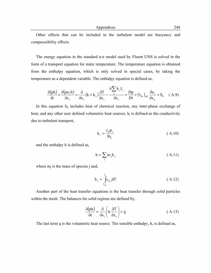
Page 1
Influences of catalyst particle geometry on fixed bed
reactor near-wall heat transfer using CFD
by
Michiel Nijemeisland
A Thesis
submitted to the Faculty of the
Worcester Polytechnic Institute
in partial fulfillment of the requirements for the
Degree of Doctor of Philosophy
in Chemical Engineering
_____________________
January 2003
Approved:
Prof. Dr. Anthony G. Dixon, Major advisor
Dr. E. Hugh Stitt, Co-Advisor, Synetix (Johnson Matthey)
Prof. Dr. Ravindra Datta, Head of Department
Page 2
ii
Summary
Fixed bed reactors are an essential part of the chemical industry as they are used in a
wide variety of chemical processes. To better model these systems a more fundamental
understanding of the processes taking place in a fixed bed is required.
Fixed bed models are traditionally based on high tube-to particle diameter ratio (N)
beds, where temperature and flow profile gradients are mild and can be averaged. Low-N
beds are used in extremely exo- and endothermic processes on the tube side of tube and
shell type reactors. In these beds, heat transfer is one of the most important aspects. The
importance of accurate modeling of heat transfer and its dependence on accurate
modeling of the flow features leads to the need for studying the phenomena in these low-
N beds in detail.
In this work a comparative study is made of the influence of spherical and cylindrical
packing particle shapes, positions and orientations on the rates of heat transfer in the
near-wall region in a steam reforming application. Computational Fluid Dynamics (CFD)
is used as a tool for obtaining the detailed flow and temperature information in a low-N
fixed bed. CFD simulation geometries of discrete particle packed beds are designed and
methods for data extraction and analysis are developed.
After conceptual and quantitative analysis of the simulation data it is found that few
clear relations between the complex phenomena of flow and heat transfer can be easily
identified. Investigated features are the orientations of the particle in the flow, and many
design parameters, such as the number and size of longitudinal holes in the particle and
external features on the particle. We find that many of the investigated features are
related and their individual influences could not be isolated in this study. Some of the
Page 3
Summary iii
related features are, for example, the number of holes in the particle design and the
particle orientation in the flow.
Some general conclusions could be drawn. External features on the particles enhance
the overall heat transfer properties by better mixing of the flow field. When holes are
present in the cylindrical particle design, heat transfer effectiveness can be improved with
fewer larger holes.
After identifying the packing-related features influencing the near-wall heat transfer
under steam reforming conditions, an attempt was made to incorporate the steam
reforming reaction in the simulation. In the initial attempts the reaction was modeled as
an energy flux at the catalyst particle surfaces. This approach was based on the abilities
of the CFD code, but turned out not accurate enough. Elimination of the effects of local
reactant depletion and the lack of solid energy conduction in the catalyst particles
resulted in an unphysical temperature field.
Several suggestions, based on the results of this study, are made for additional aspects
of particle design to be investigated. Additionally, suggestions are made on how to
incorporate the modeling of a reaction in fixed bed heat transfer simulations.
Page 4
iv
Acknowledgments
The work you see before you is the latest result of a project that grew out of a series of
exchanges of chemical engineering students from the University of Twente to Worcester
Polytechnic Institute. Throughout these exchanges particle packed beds, the
computational modeling thereof and coffee have been essential parts. As the latest, and
perhaps last, of the participants in these exchanges I take pride in presenting this work,
but will not take all the blame myself, as I thank all the people that made this possible.
First and foremost I would like to thank my advisor, Prof. A.G. Dixon for continued
scientific, financial, and moral support, as well as for creating the possibility for the
student exchanges. Then I would like to thank all the additional participants in the
student exchanges. Emeritus Prof. K.R. Westerterp at the University of Twente for
organizing this exchange on the Dutch side, Hans van Dongeren, Olaf Derkx, and Simon
Logtenberg for keeping the dream alive and Peter Roos for introducing me to Simon and
informing me of the opportunities at WPI.
After the introductory part of the project, which became my Masters Thesis in which
CFD was shown to be a viable simulation method for particle packed beds, we were able
to attract external support. With the external support, the project acquired a definite
amount of direction and clear goals. Additionally it supplied a member of the thesis
committee, Dr. E.H. Stitt. I am grateful to Synetix for the financial support and in
specific Dr. Stitt for convincing the company that this project is worth sponsoring, as
well as scientific, and moral support combined with relentless enthusiasm towards the
possibilities and capabilities of CFD modeling.
With the combination of the Masters project and the PhD I have spend almost six
years at Worcester Polytechnic Institute and have enjoyed every moment of my time
Page 5
Acknowledgments v
here. The pleasant atmosphere at the chemical engineering department combined with the
interesting group of people employed, and studying there, are major players in this. In the
six years I have been a part of the department I have had the good fortune to work with a
large number of these people, and I would like to thank them for making the experience
enjoyable. Within the faculty I would especially like to thank department head Prof. R.
Datta for taking a position in my thesis committee. Within the graduate student body I
would like to thank some of the hardcore WPI chemical engineers, people that have been
a part of my academic experience for most of my stay at WPI, Erik Engwall, Ipek Guray,
Yoojeong Kim, Chris Heath, and Arjan Giaya. Also I am thankful to the people who
were at WPI for only a fraction of my stay, but formed my experience no less than
anyone else, thanks, Jason Wiley, Craig Thompson, Sean Emerson, Kathy Pacheco,
Kellie Martin, Tony Thampan, Faisal Syed, Manuela Serban, Josef Find, Paolo Paci,
Federico Guazzone, and many many more.
Besides the academic experience there were many more people who defined my life in
the last six years, I am very grateful to them. A big thank you goes to all the people that
have tolerated me while we were roommates, thanks Chris Wieczorek, Fred Souret, Uta
Dieregsweiler and Andrew Roberts. Another big thank you goes to the Dutch clan who
introduced me to peculiarities of Worcester, and New England, thanks, Simon, Mirjam,
Kathy, and Otto. I would also like to thank all my new friends in New England, and
surroundings, who played such a big role in the overall experience. I would especially
like to thank, John Valiulis, the super-connector, Paul and Krista Andry for being an
excellent NYC connection, and great friends, Jon Eisenberg for allowing the ‘foreigner’
to play with the Bombers, as well as the rest of the team.
By performing graduate studies in the United States I left behind a good deal of
friends and family in the Netherlands. The new friends and colleagues in the States made
it easy and enjoyable for me to adapt to a different way of life. The friends I left in the
Netherlands made it possible for me to keep in touch with things back home. Thank you,
Andre, Annemarie, Bas, Brigitte, Dolf, Eduard, Gerben, Ieke, Jacco, Krista, Paul, Pascal,
and Pieter.
Page 6
Acknowledgments vi
Last but by no means least I would like to thank my parents and my brother for their
support in my choices; they made me who I am today, thank you very much.
Then there is one person who is hard to categorize, a special thank you goes to my
colleague, roommate, fellow Dutch clan member, and very good friend Ivo Krausz.
Thanks, everybody.
Page 7
vii
Table of Contents
Summary......................................................................................................................... ii
Acknowledgments ......................................................................................................... iv
List of Figures ............................................................................................................... ix
List of Tables..............................................................................................................xvii
1. Introduction ............................................................................................................. 1
1.1 Problem Statement............................................................................................. 1
1.2 Background ....................................................................................................... 2
1.3 Literature ........................................................................................................... 9
1.4 Computational Fluid Dynamics....................................................................... 24
1.5 Validation ........................................................................................................ 48
2. Simulation Geometry Development...................................................................... 55
2.1 Deciding on geometry size .............................................................................. 55
2.2 N = 4 sphere geometries .................................................................................. 59
2.3 Near-wall segment geometries ........................................................................ 74
3. CFD Data Analysis – Sphere Geometry ............................................................... 94
3.1 Thermal analysis.............................................................................................. 95
3.2 Flow analysis ................................................................................................. 106
3.3 Relating flow and energy analyses................................................................ 120
4. Effects of Particle Geometry ............................................................................... 133
4.1 Model designs................................................................................................ 133
4.2 Conceptual analysis ....................................................................................... 145
4.3 Quantitative data analysis.............................................................................. 191
Page 8
Table of Contents viii
5. Modeling a Steam Reforming Reaction .............................................................. 208
5.1 Steam reforming reaction .............................................................................. 208
5.2 User defined code.......................................................................................... 212
5.3 Reaction modeling results ............................................................................. 214
5.4 Concluding remarks ...................................................................................... 218
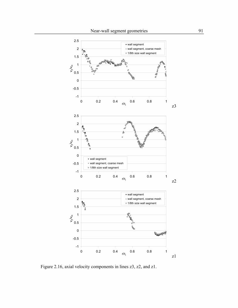
6. Conclusions and Recommendations.................................................................... 219
6.1 Conclusions ................................................................................................... 219
6.2 Recommendations ......................................................................................... 224
Nomenclature ............................................................................................................. 233
Literature References ................................................................................................. 236
Appendices ................................................................................................................. 245
Appendix 1: The standard κ-ε turbulence model ................................................... 246
Appendix 2: Geometric design in GAMBIT.......................................................... 250
Appendix 3: From mesh to case in Fluent UNS..................................................... 253
Appendix 4: Full-bed wall-segment flow comparisons ......................................... 256
Appendix 5: UDF code for simple steam reforming reaction in fluent.................. 267
Page 9
ix
List of Figures
Figure 1.1. typical examples of a) the surface mesh on a number of spheres and a section
of the cylinder and b) a section of the interior mesh in a plane indicated in part a. . 38
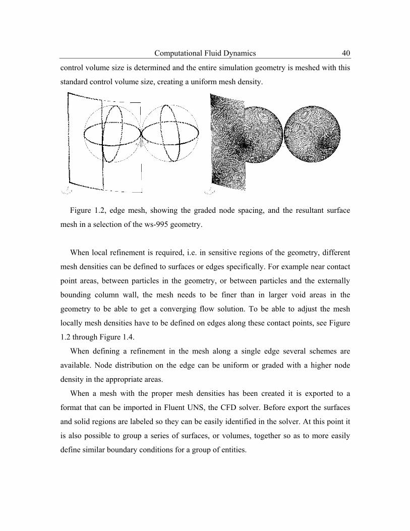
Figure 1.2, edge mesh, showing the graded node spacing, and the resultant surface mesh
in a selection of the ws-995 geometry....................................................................... 40
Figure 1.3, selected control volumes in the ws-995 mesh interpolated from the node
spacing and surface mesh shown in Figure 1.2......................................................... 41
Figure 1.4, two-dimensional display and a detail of the control volumes in the fluid
region of the ws-995 mesh showing the size grading. .............................................. 41
Figure 1.5. velocity vector plot as obtained from Fluent UNS, vectors colored by axial
velocity component [m/s].......................................................................................... 47
Figure 1.6, experimental setup and detail of the thermocouple cross, with the radial
positions of the thermocouples indicated, used for temperature data collection. ..... 49
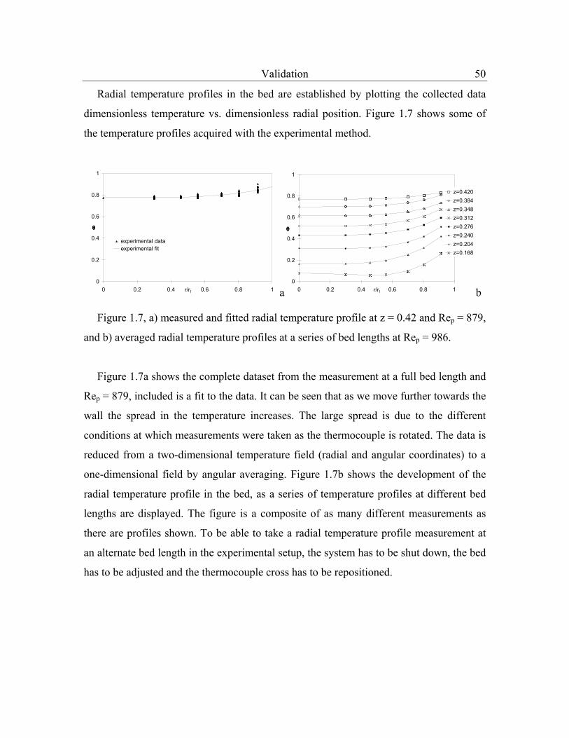
Figure 1.7, a) measured and fitted radial temperature profile at z = 0.42 and Rep = 879,
and b) averaged radial temperature profiles at a series of bed lengths at Rep = 986.50
Figure 1.8, the layout of the CFD geometry of an N = 2 bed, used for the validation
study; a) shows the bottom section of the bed, b) shows the top view of the bed. ... 51
Figure 1.9, radial temperature profiles acquired by CFD simulation for a) z = 0.42 and
Rep = 1922, and b) a series of axial positions at Rep = 986. ..................................... 52
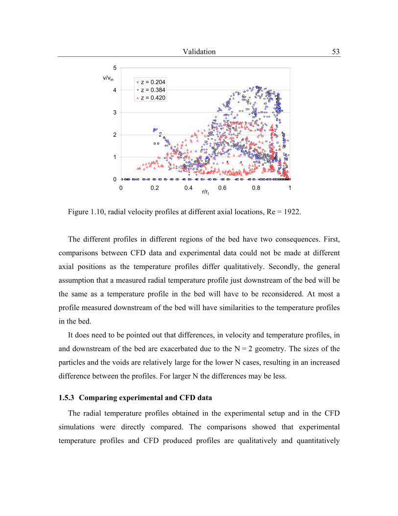
Figure 1.10, radial velocity profiles at different axial locations, Re = 1922. ................... 53
Figure 1.11, direct comparisons of experimental and CFD temperature profiles at z = 0.42
for a) Rep = 986, and b) Rep = 1922.......................................................................... 54
Figure 2.1, photograph (a) of the bottom layer of spheres and (b) the modified version
with the locations of the spheres specified................................................................ 63
Page 10
List of Figures x
Figure 2.2, two axially adjacent 9-sphere wall layers....................................................... 67
Figure 2.3, axial spacing between adjacent wall layers. ................................................... 68
Figure 2.4, the spiraling center structure simulated in an N = 2.15 bed. .......................... 70
Figure 2.5, the initial wall-segment geometry, top view and isometric view. .................. 75
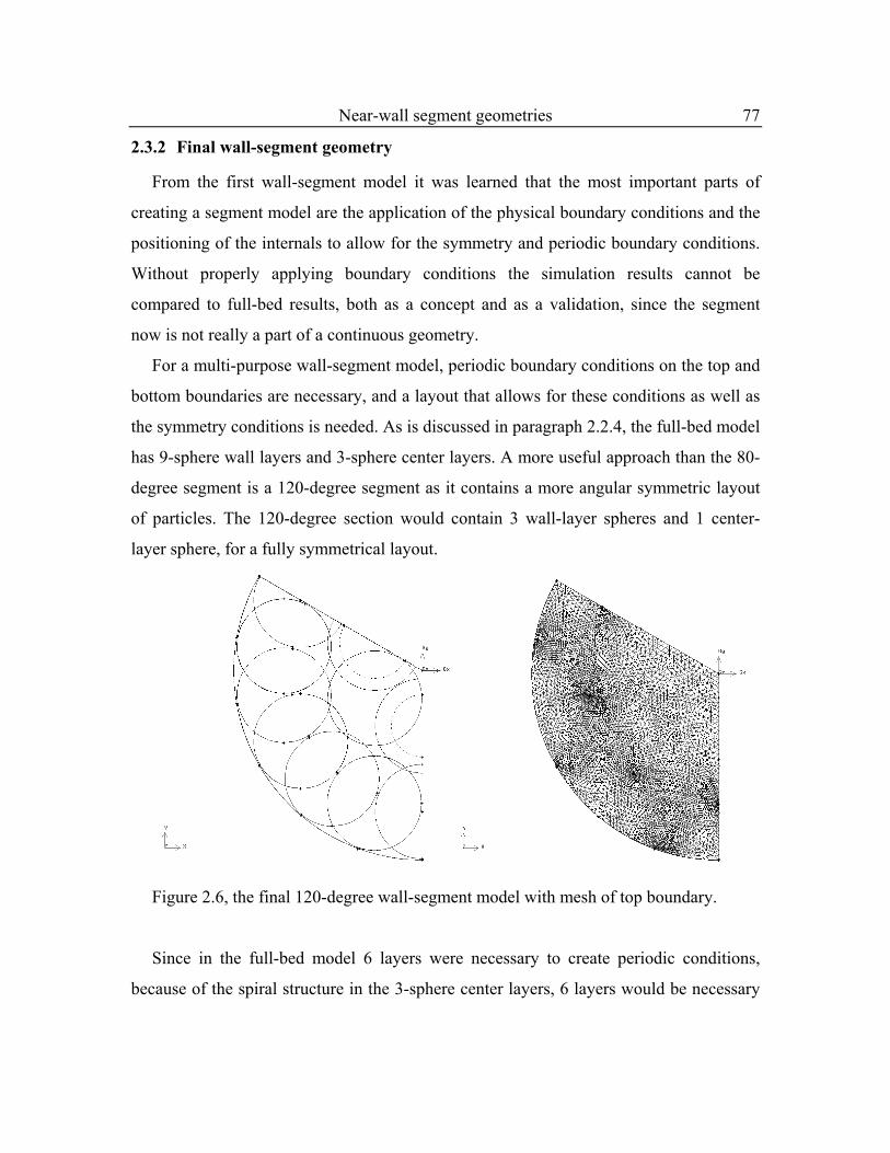
Figure 2.6, the final 120-degree wall-segment model with mesh of top boundary. ......... 77
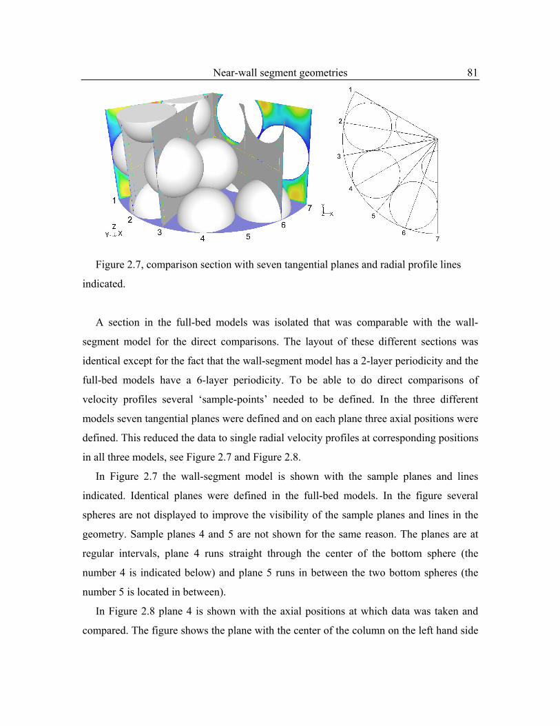
Figure 2.7, comparison section with seven tangential planes and radial profile lines
indicated. ................................................................................................................... 81
Figure 2.8, plane 4 with the axial data lines...................................................................... 82
Figure 2.9, velocity vectors in plane 4 for the three different models a) no-sphere-mesh b)
re-mesh c) wall-segment model. ............................................................................... 84
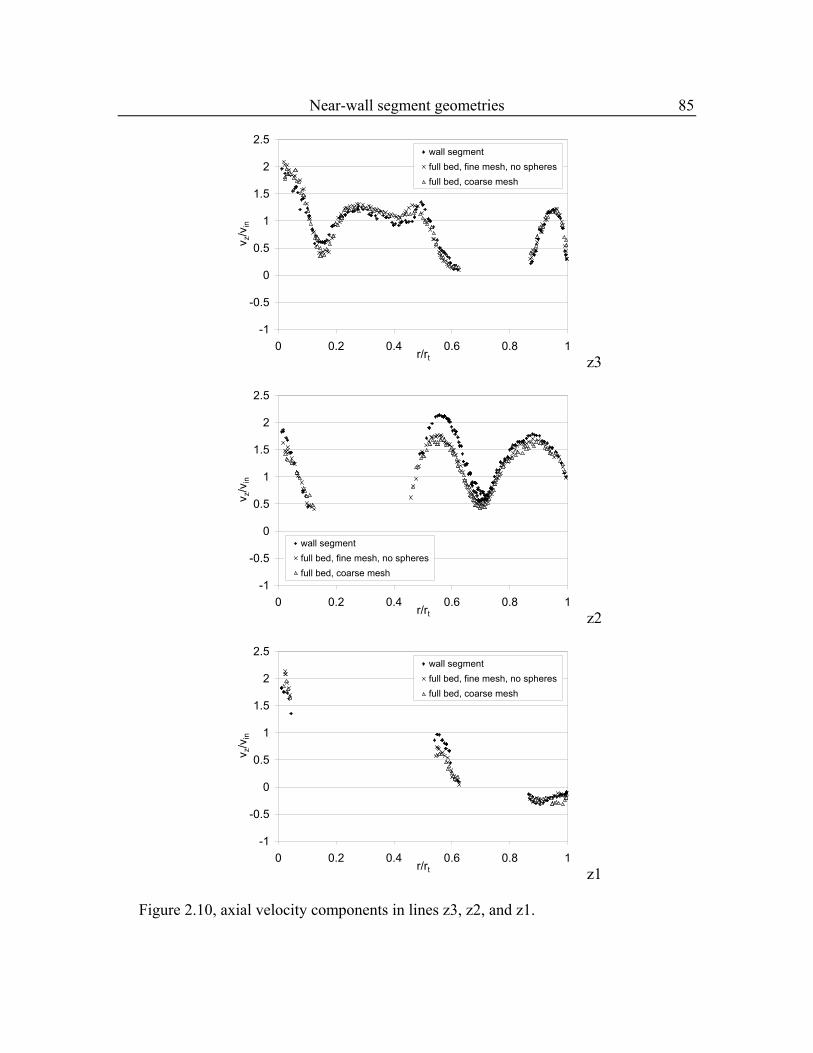
Figure 2.10, axial velocity components in lines z3, z2, and z1......................................... 85
Figure 2.11, radial velocity components in lines z3, z2, and z1. ...................................... 86
Figure 2.12, tangential velocity components in lines z3, z2 and, z1................................. 87
Figure 2.13, axial velocity profiles in z1 of plane 3 and plane 5 respectively.................. 88
Figure 2.14, tangential velocity profiles in z1 of plane 3 and plane 5 respectively.......... 89
Figure 2.15, radial and tangential velocities in z1 of plane 1. .......................................... 89
Figure 2.16, axial velocity components in lines z3, z2, and z1......................................... 91
Figure 2.17, radial velocity components in lines z3, z2, and z1. ...................................... 92
Figure 2.18, tangential velocity components in lines z3, z2, and z1................................. 93
Figure 3.1, contour maps of the complete temperature field in the x = 0 plane of the n = 2
geometry at varying fluid velocities, Rep is respectively 373, 986 and 1922. .......... 97
Figure 3.2, temperature contour maps of respectively the x = 0 plane of the first stage in
the N = 4 geometry stacking, and the y = 0 plane of the fourth stage. Main axial flow
direction moves from left to right in these pictures. ................................................. 98
Figure 3.3, composite of temperature contour maps of the x = 0 plane from four separate
simulations in the N = 4 geometry. Main axial flow direction moves from left to
right in these pictures, Rep = 1000. ........................................................................... 99
Page 11
List of Figures xi
Figure 3.4, thermal conductivities, kr/kf, and wall heat transfer coefficients, Nuw,
determined from different samplings of the CFD data for the N = 2 geometry
simulations. ............................................................................................................. 101
Figure 3.5, velocity vector plot of the flow field in plane 4, vectors colored by axial
velocity component [m/s]........................................................................................ 107
Figure 3.6, velocity vectors in the wall-segment geometry, vectors are colored by axial
velocity [m/s]........................................................................................................... 109
Figure 3.7, flow pathlines of the flow field in plane 4, pathlines are colored by axial
velocity [m/s]........................................................................................................... 110
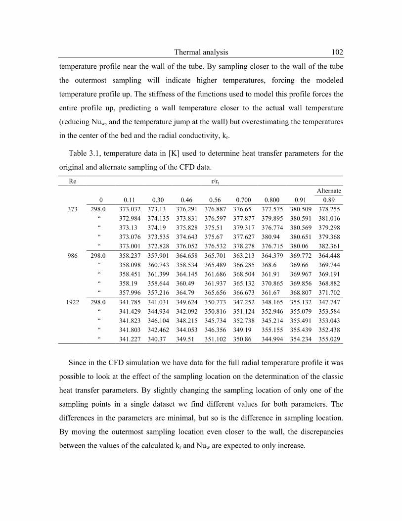
Figure 3.8, top view of the flow pathlines in plane 4, showing the three-dimensional
quality of the pathlines, pathlines are colored by axial velocity [m/s]. .................. 111
Figure 3.9, pathlines in the wall-segment geometry, pathlines are colored by axial
velocity [m/s]........................................................................................................... 112
Figure 3.10, pathlines in the wall-segment geometry, focusing on the wake flow,
pathlines are colored by axial velocity [m/s]. ......................................................... 113
Figure 3.11, histograms of the volumetric flux distributions in the N = 2 simulation
geometry flow field. ................................................................................................ 115
Figure 3.12, local and cumulative porosities in the depicted planar geometry determined
algebraically and with CFD data............................................................................. 116
Figure 3.13, velocity contour plots of respectively the velocity magnitude and the axial
component of the velocity in plane 4, velocities in [m/s]. ...................................... 117
Figure 3.14, velocity contour plots of respectively the radial and tangential velocity
components in plane 4, velocities in [m/s].............................................................. 117
Figure 3.15, wall heat flux map on the cylinder wall of the wall segment model, in
[kW/m2]. The repetitive structure is indicated by the gridlines. ............................. 123
Figure 3.16, parallel projection of the wall segment model, indicating the regularity of the
wall structure. .......................................................................................................... 123
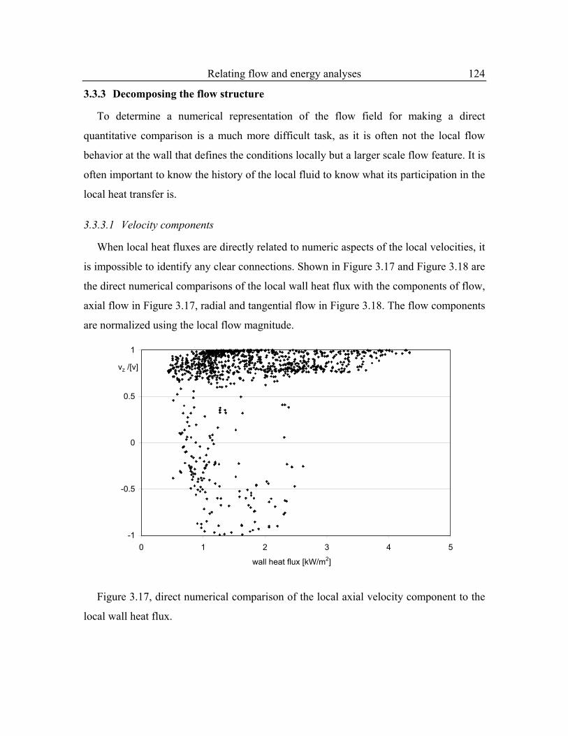
Figure 3.17, direct numerical comparison of the local axial velocity component to the
local wall heat flux. ................................................................................................. 124
Page 12
List of Figures xii
Figure 3.18, direct numerical comparison of the local radial and tangential velocity
components to the local wall heat flux.................................................................... 125
Figure 3.19, direct numerical comparison of the normalized local x and y vorticity
components to the local wall heat flux.................................................................... 126
Figure 3.20, direct numerical comparison of the normalized local z vorticity component
and the vorticity magnitude to the local wall heat flux........................................... 127
Figure 3.21, direct numerical comparison of the local fluid helicity to the local wall heat
flux. ......................................................................................................................... 128
Figure 3.22, the axial derivative of the axial velocity component related to the local wall
heat flux................................................................................................................... 129
Figure 3.23, the radial and tangential derivatives of the axial velocity components related
to the local wall heat flux. ....................................................................................... 130
Figure 3.24, the unit-cell section used for comparing fluid flow to wall heat flux, a) the
flow field expressed in pathlines, b) the simplified expression of the flow field in the
fluid section, c) relative wall heat flux in ten gradations. All three are displayed from
the viewpoint of an observer looking at the tube wall from outside the bed. ......... 131
Figure 4.1, isometric views of the 4-hole particle........................................................... 136
Figure 4.2, isometric views of the 3-hole particle........................................................... 136
Figure 4.3, isometric views of the 1-hole particle........................................................... 137
Figure 4.4, isometric views of the 4smholes particle...................................................... 137
Figure 4.5, isometric views of the grooves particle. ....................................................... 138
Figure 4.6, isometric views of the 1bighole particle. ...................................................... 139
Figure 4.7, experimental results of random dense packing of 1:1 cylindrical particles in
an N = 4 bed. ........................................................................................................... 140
Figure 4.8, the base bed geometry with the standard 4-hole particles, ws-4hole-1b. ..... 141
Figure 4.9, additional bed geometries a) ws-4hole-2 and b) ws-4hole-3........................ 142
Figure 4.10, wall adjacent particle numbering in the three different bed geometries..... 147
Figure 4.11, contour plot of axial fluid velocities in the r=0.045 plane of the ws-4hole-1b
geometry, colored by axial velocity in [m/s]. ......................................................... 149
Page 13
List of Figures xiii
Figure 4.12, selected pathlines released in the r=0.045 plane in the ws-4hole-1b
geometry, colored by axial velocity in [m/s]. ......................................................... 149
Figure 4.13, selected pathlines released in the r=0.05 plane in the ws-4hole-1b geometry,
colored by axial velocity in [m/s]............................................................................ 150
Figure 4.14, column wall temperature map for the base 4-hole cylinder packing, ws-
4hole-1b, scale in [K]. ............................................................................................. 150
Figure 4.15, contour plot of axial fluid velocities in the r=0.045 plane of the ws-4hole-2
geometry, colored by axial velocity in [m/s]. ......................................................... 153
Figure 4.16, selected pathlines released in the r=0.045 plane in the ws-4hole-2 geometry,
colored by axial velocity in [m/s]............................................................................ 153
Figure 4.17, selected pathlines released in the r=0.05 plane in the ws-4hole-2 geometry,
colored by axial velocity in [m/s]............................................................................ 154
Figure 4.18, column wall temperature map for the first alternate 4-hole cylinder packing,
ws-4hole-2, scale in [K]. ......................................................................................... 154
Figure 4.19, contour plot of axial fluid velocities in the r=0.045 plane of the ws-4hole-3
geometry, colored by axial velocity in [m/s]. ......................................................... 157
Figure 4.20, selected pathlines released in the r=0.045 plane in the ws-4hole-3 geometry,
colored by axial velocity in [m/s]............................................................................ 157
Figure 4.21, selected pathlines released in the r=0.045 plane in the ws-4hole-3 geometry,
colored by axial velocity in [m/s]............................................................................ 158
Figure 4.22, column wall temperature map for the second alternate 4-hole cylinder
packing, ws-4hole-3, scale in [K]. .......................................................................... 158
Figure 4.23, column wall temperature maps for the four different particle designs,
temperature scales are normalized to the largest range in [K]. ............................... 162
Figure 4.24, column wall temperature maps for the four different particle designs,
temperature scales are normalized to the smallest range in [K].............................. 163
Figure 4.25, comparison of flow situations related to particles with a different amount of
holes, section 1; pathlines are colored by axial velocities in [m/s], scale to the left of
each figure. .............................................................................................................. 165
Page 14
List of Figures xiv
Figure 4.26, comparison of flow situations related to particles with a different amount of
holes, section 2; pathlines are colored by axial velocity in [m/s], scale to the left of
each figure. .............................................................................................................. 167
Figure 4.27, comparison of flow situations related to particles with a different amount of
holes in section 3; pathlines are colored by axial velocity in [m/s], scale to the left of
each figure. .............................................................................................................. 169
Figure 4.28, comparison of flow situations related to particles with a different amount of
holes in section 4; pathlines are colored by axial velocity in [m/s], scale to the left of
each figure. .............................................................................................................. 170
Figure 4.29, temperature maps for the four different geometries with varying hole sizes,
scale in [K]. ............................................................................................................. 172
Figure 4.30, comparison of flow situations in the 4hole and 4smholes geometries in
section 1; pathlines are colored by axial velocity in [m/s], scale to the left of each
figure. ...................................................................................................................... 173
Figure 4.31, comparison of flow situations in the 4hole and 4smholes geometries in
sections 3 and 4; pathlines are colored by axial velocity in [m/s], scale to the left of
each figure. .............................................................................................................. 174
Figure 4.32, comparison of flow situations in the 1hole and 1bighole geometries in
section 1; pathlines are colored by axial velocity in [m/s], scale to the left of each
figure. ...................................................................................................................... 175
Figure 4.33, comparison of flow situations in the 1hole and 1bighole geometries in
section 2; pathlines are colored by axial velocity in [m/s], scale to the left of each
figure. ...................................................................................................................... 176
Figure 4.34, comparison of flow situations in the 4hole and 1bighole geometries in
sections 2 and 3; pathlines are colored by axial velocity in [m/s], scale to the left of
each figure. .............................................................................................................. 178
Figure 4.35, temperature maps for the 4hole and grooves geometries, scale in [K]....... 181
Figure 4.36, comparison of flow situations in the 4hole and grooves geometries in section
1; pathlines are colored by axial velocity in [m/s], scale to the left of each figure. 181
Page 15
List of Figures xv
Figure 4.37, comparison of flow situations in the 4hole and grooves geometries in
sections 2 and 3; pathlines are colored by axial velocity in [m/s], scale to the left of
each figure. .............................................................................................................. 183
Figure 4.38, comparison of flow situations in the 4hole and grooves geometries in section
4; pathlines are colored by axial velocity in [m/s], scale to the left of each figure. 184
Figure 4.39, temperature maps for the three different simulated reactor conditions, scale
in [K]. ...................................................................................................................... 187
Figure 4.40, pathline plots for the three simulated reactor conditions, pathlines are
colored by axial velocity in [m/s], scale to the left of each figure. ......................... 188
Figure 4.41, continuous radial temperature profile comparisons.................................... 192
Figure 4.42, radial temperature profiles and average wall temperatures for the three
different orientations of the 4-hole particle bed...................................................... 195
Figure 4.43, radial temperature profiles and average wall temperatures for the series of
particle designs with different number of longitudinal holes.................................. 197
Figure 4.44, radial temperature profiles and average wall temperatures for the series with
different hole diameters........................................................................................... 200
Figure 4.45, radial temperature profiles and average wall temperatures for the 4hole and
big-hole particle beds with identical bed porosities................................................ 202
Figure 4.46, averaged radial temperature profiles for the standard and grooved particles.204
Figure 4.47, averaged radial porosity profiles in the solid cylinder, standard 4hole and
grooves geometries.................................................................................................. 205
Figure 4.48, normalized and regular radial temperature profiles, and average wall
temperatures for the runs at different reactor conditions. ....................................... 206
Figure 5.1, contour plots of the heat flux on the particle surfaces, showing the entire
range of sink magnitudes on the left and a cropped range on the right. ................. 216
Figure 5.2, temperature profiles on the particle surfaces in the reaction simulation, scale
in [K]. Inset: contour plot of axial flow velocities in the center plane of the
geometry, scale in axial velocity magnitude [m/s].................................................. 217
Page 16
List of Figures xvi
Figure 6.1, relative hole sizes of respectively the standard hole, small hole, and the
suggested pinhole and large hole particles.............................................................. 226
Figure A. 1, top view of the wall segment geometry, with the planes for comparisons
indicated. ................................................................................................................. 256
Figure A. 2, layout plots of the 6 comparison planes, illustrating the similarities between
the layout of planes 3 and 5, 2 and 6, and 1 and 7 respectively. ............................. 257
Figure A. 3, axial velocity comparisons in planes 3 and 5. ............................................ 258
Figure A. 4, radial velocity comparisons in planes 3 and 5. ........................................... 259
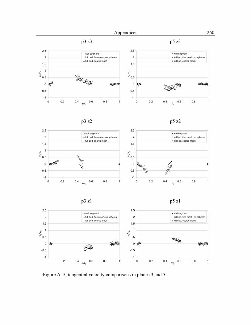
Figure A. 5, tangential velocity comparisons in planes 3 and 5. .................................... 260
Figure A. 6, axial velocity comparisons in planes 2 and 6. ............................................ 261
Figure A. 7, radial velocity comparisons in planes 2 and 6. ........................................... 262
Figure A. 8, tangential velocity comparisons in planes 2 and 6. .................................... 263
Figure A. 9, axial velocity comparisons in planes 1 and 7. ............................................ 264
Figure A. 10, radial velocity comparisons in planes 1 and 7. ......................................... 265
Figure A. 11, tangential velocity comparisons in planes 1 and 7. .................................. 266
Page 17
xvii
List of Tables
Table 2.1, coordinates for the wall layer spheres in the first layer, in inches................... 67
Table 2.2, coordinates for the wall layer spheres in the second layer, in inches .............. 67
Table 2.3, sizes of the different simulation geometries in million control volumes. ........ 78
Table 2.4, size comparison of the meshes used for flow profile comparisons.................. 80
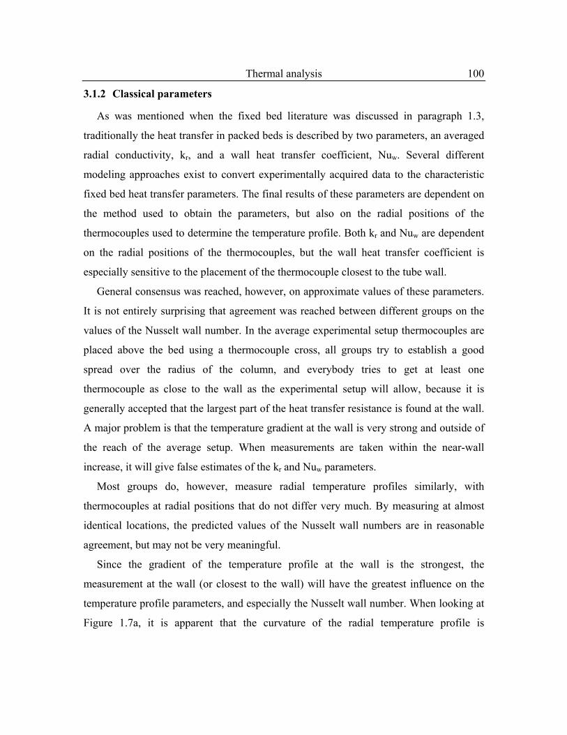
Table 3.1, temperature data in [K] used to determine heat transfer parameters for the
original and alternate sampling of the CFD data. ................................................... 102
Table 3.2, differences in the boundary conditions between the laboratory and reforming
conditions. ............................................................................................................... 103
Table 4.1, overview of simulation series for the investigation of the effects of the particle
geometry.................................................................................................................. 134
Table 4.2, 4-hole catalyst particle dimensions. ............................................................... 135
Table 4.3, boundary conditions and fluid properties for the three reactor conditions. ... 143
Table 4.4, comparing overall heat capacities and energy required to increase the
temperature of the geometries. ................................................................................ 193
Table 4.5, wall temperature distributions in the geometries with particles with a different
number of holes. ...................................................................................................... 198
Table 4.6, wall temperature distributions in the geometries with particles with different
hole sizes. ................................................................................................................ 200
Table 5.1, reactions included in the simplified reaction model, with equilibrium constants
and reaction enthalpies. ........................................................................................... 209
Table 5.2, activation energies, adsorption enthalpies and pre-exponential factors for the
reaction model. ........................................................................................................ 211
Table 6.1, the suggested broadening in the orientations, and number of holes series. ... 225
Page 18
List of Figures xviii
Table 6.2, the suggested expansion in the hole-size series. ............................................ 226
Table 6.3, the suggested expansion in the porosity series. ............................................. 226
Table 6.4, the suggested expansion in investigating the effect of external features. ...... 227
Table A. 1, placement of the particles in the different bed geometries. ......................... 252
Page 19
1
1. Introduction
1.1 Problem Statement
Fixed bed reactors are an essential part of the chemical industry as they are used in a
wide variety of chemical processes. For design of fixed bed reactors, application of
several models is required to be able to describe the different physical and chemical
processes taking place in the reactor. The trend in most of these models has always been
towards providing grouped parameters for easy description of the physical processes,
sometimes combining several physical processes in a single parameter. The main
problem with these methods is the lack of universality of the used models, resulting in the
development of a multitude of models and modeling parameters for specific reactors used
in specific processes.
To better model these systems a more fundamental understanding of the processes
taking place in a fixed bed is required. To obtain better understanding it is first necessary
to be able to obtain accurate data from inside the fixed bed. In an earlier study we have
shown that Computational Fluid Dynamics (CFD) is an accurate, reliable, and non-
intrusive method that can provide a wealth of data in low tube-to-particle diameter ratio
(N) fixed beds (Nijemeisland and Dixon, 2001). CFD can provide us with detailed
information on flow processes and heat and mass transfer processes. This is a tremendous
advantage over traditional methods of obtaining flow and heat transfer data in fixed beds,
which are usually limited to few sampling points and are mostly intrusive.
Experimentally it is very difficult to obtain data in the near-wall region of a fixed bed,
which has resulted in several model adaptations to be able to relate experimentally
acquired data to the model. In general, experimental data, when extrapolated to the wall,
Page 20
Introduction 2
predict a temperature at the wall considerably lower than the wall temperature, due to the
laminar wall layer, decreased solid conduction, and reduced radial dispersion of heat.
This discrepancy is then resolved with an idealized temperature jump at the wall
described by hw, the wall heat transfer coefficient. This parameter is used to describe a
phenomenon (the temperature jump at the wall) that is not physically present but which,
based on experimental results, cannot be described any more accurately. CFD offers
more detailed data and better insight in the transport phenomena in the near-wall region.
This combination may eventually lead to a more fundamental way of modeling the near-
wall heat transfer, eliminating the need for the empirical parameter hw.
Low-N beds are used in extremely exo- and endothermic processes in tube and shell
type reactors. In these setups heat transfer is one of the most important aspects, especially
at the tube wall; combined with high fluid throughput the near-wall heat transfer
resistance becomes dominant. In this specific type of setup the modeling of the near-wall
heat transfer with a single parameter, hw, is very questionable.
In this work a comparative study will be made of the influence of the particle shapes,
positions and orientations on the rates of heat transfer in the near-wall region in low-N
fixed beds.
1.2 Background
A good qualitative understanding and an accurate quantitative description of fluid
flow and heat transfer in fixed beds are necessary for the modeling of these devices.
Accurate modeling of these fixed beds is complicated, especially in low tube to particle
diameter ratios (N), in the range of 3-8, due to the presence of wall effects across the
entire radius of the bed. With new methods such as CFD it is possible to get a detailed
view of the flow behavior in these beds.
In this study the steam reforming process is selected as an example for industrial
application of CFD in a fixed bed with a low tube-to-particle diameter ratio. By applying
the work to an industrial process we can utilize the versatility of the CFD method and
show its applicability to practical situations. The steam reforming process was chosen for
Page 21
Introduction 3
a number of reasons. The types of geometries used in steam reforming resemble the types
of geometries on which the validation study, described in paragraph 1.5, was performed.
The optimization progress in steam reforming can be helped by a more fundamental
study of the processes taking place in the steam reforming bed, CFD is an optimal tool
for providing data where other methods are not available.
1.2.1 Introduction of the steam reformer and its problems
Steam reforming is a widely used method in industry for the production of synthesis
gas. Synthesis gas is a mixture of hydrogen gas and carbon monoxide, which is used in
many processes. The exact composition of the produced synthesis gas, i.e. the ratio of
hydrogen to carbon monoxide and the amount of other species, such as carbon dioxide,
water, methane and various side products such as nitrous oxides and other traces,
depends on the type of steam reforming process, the ratio of the reagents, the catalyst
used and the reactor conditions. Sometimes the creation of synthesis gas is the primary
goal, in for example the production of hydrogen. Other times synthesis gas is produced as
a precursor for further production, mostly as hydrogen production for Fischer-Tropsch
processes, or methanol, or ammonia synthesis.
An industrial size steam reformer generally has a tube and shell design, typically
housing up to 400 0.1 m inner diameter, 13 m loaded length tubes. The exact
specifications are, of course, process dependent. The highly endothermic reaction is
taking place in the catalyst filled tubes. The shell side is used for supply of energy to the
tubes, usually in the form of a series of burners. The steam reformer is operated at very
high temperatures, approximately 1000 K, and very high reactant throughput. The base
reaction in steam reforming is:
224 H3COOHCH +↔+ ( 1.1)
Simultaneously the water gas shift reaction is taking place:
222 HCOOHCO +↔+ ( 1.2)
Page 22
Introduction 4
The overall process is highly endothermic, even though the water gas shift reaction is
slightly exothermic. The heat of reaction for reaction ( 1.1) ∆H = +206.1 kJ/mol, and for
reaction ( 1.2) ∆H = -45.15 kJ/mol (Xu and Froment, 1989).
The main issue in the design of steam reformers is that heat is supplied to the reactant
mixture as fast and as efficiently as possible; thus supplying the reaction with the energy
it needs. Both the endothermic reaction and the high reactant throughput will put strains
on the supply of energy.
Experimentally very little data can be acquired at steam reformer tube conditions. The
high temperature and the high flow conditions make measurement of either temperature
or flow patterns very difficult. Currently the only experimental data that can be obtained
inside industrial tube and shell steam reformers are pyrometer measurements of the
external tube temperature. This method only gives a superficial indication of the internal
situation but can already identify problems inside the reformer. It can identify problem
areas in heat absorption in the tube banks. When, for example, a patch of catalyst has
deactivated, or due to non-uniform packing heat consumption in a particular area is
reduced, hot spots will show up in the tube banks. These hot spots exert thermal strain on
the reformer-tubes, which will lead to reduced operation time. Only problem areas can be
identified with the pyrometer measurement. To be able to understand the principles
behind the heat transfer problems inside the tubes more data is required.
This is an area where CFD can give a lot more information easily and without
disturbance of the temperature and flow field. Using CFD we can identify heat transfer
and flow patterns inside the tubes, look at the effects of catalyst degradation and at the
effects of particle stacking, orientation or shape.
From numerous studies by reforming catalyst producers it has been shown that
catalyst particle shapes influence the heat transfer into the reformer-tube. Certain aspects
of the catalyst particle design may positively influence the heat transfer from the shell
side to the tube side. The only currently available data in this area has been empirically
collected and correlated. The optimal design of the catalyst particle has been established
by trial and error in pilot plant scale setups. CFD might give us insight into the changes
Page 23
Introduction 5
in flow and heat transfer properties related to a catalyst particle shape and its position in
the reformer-tube. Proper analysis of the heat transfer and flow processes inside the
reformer-tubes are expected to give us a better explanation of the overall heat transfer
into the tubes.
1.2.2 CFD in general
Using CFD, to create better understanding in flow processes, is an essential step, as it
will provide us with information that cannot be obtained in any other way. It is therefore
essential to further explore the concept CFD, what is CFD? And how can we use CFD to
provide us with the information we desire?
Computational Fluid Dynamics is a method that is becoming more and more popular
in the modeling of flow systems in many fields. CFD codes make it possible to
numerically solve flow, mass and energy balances in complicated flow geometries. The
results show specific flow and heat transfer patterns that are hard to obtain
experimentally or with conventional modeling methods.
CFD numerically solves the Navier-Stokes equations and the energy and species
balances. The differential forms of these balances are solved over a large number of
control volumes. These control volumes are small volumes within the flow geometry, all
control volumes properly combined form the entire flow geometry. The size and number
of control volumes (mesh density) is user determined and will influence the accuracy of
the solutions, to a certain degree. After boundary conditions have been implemented, the
flow and energy balances are solved numerically; an iteration process decreases the error
in the solution until a satisfactory result has been reached.
The tremendous growth in computational capabilities over the last decades has made
CFD one of the fastest growing fields of research. Areas of research where CFD has
taken an important role include the aerospace and automotive industries where CFD has
become a relatively cheap alternative to wind tunnel testing. CFD type software,
numerically solving problems over a grid of elements, although not specifically focused
Page 24
Introduction 6
on flow problems, has been used in the Civil Engineering field for stress type
calculations in construction for years.
Commercially available CFD codes use one of three basic spatial discretization
methods, finite differences (FD), finite volumes (FV) or finite elements (FE). Earlier
CFD codes used FD or FV methods and have been used in stress and flow problems. The
major disadvantage of the FD method is that it is limited to structured grids, which are
hard to apply to complex geometries and mostly used for stress calculations in beams etc.
In a three-dimensional structured grid every node is an intersection of three lines with a
respective specific x, y and z-coordinate, resulting in a grid with all rectangular elements.
The rectangular elements can undergo limited deformation to fit the geometry but the
adaptability of the grid is limited.
The FV and FE methods support both structured and unstructured grids and therefore
can be applied to a more complex geometry. An unstructured grid is a two-dimensional
structure of triangular cells or a three-dimensional structure of tetrahedral cells, which is
interpolated from respectively, user-defined node distributions on the surface edges or, a
triangular surface mesh. The interpolation part of the creation process of an unstructured
mesh is less directly influenced by the user than in a structured mesh because of the
random nature of the unstructured interpolation process. This aspect does, however,
allow the mesh to more easily adapt to a complex geometry. The FE method is in general
more accurate than the FV method, but the FV method uses a continuity balance per
control volume, resulting in a more accurate mass balance. FV methods are more
appropriate for flow situation, whereas FE methods are used more in stress and
conduction calculations, where satisfying the local continuity is of less importance.
By using CFD and an unstructured model of the fixed bed geometry in the simulation
a detailed description of the flow behavior within the bed can be established, which can
then be used in more accurate modeling. The simulation requires that a detailed model of
the desired geometry be made. The fixed bed geometry is so complex that only
unstructured type grids can be used.
Page 25
Introduction 7
1.2.3 Use of CFD in chemical and reaction engineering
Recently the range of applications for CFD has been extended to the field of Chemical
Engineering with the introduction of specially tailored fluid mixing programs. The
general setup of most CFD programs allows for a wide range of applications, several
commercial packages have introduced chemical reactions in the CFD code allowing rapid
progress of the use of CFD within the field of Chemical Reaction Engineering (Bode,
1994; Harris et al., 1996; Kuijpers and van Swaaij, 1998; Ranade, 1995). Already CFD
can be applied to the more physical aspects of Chemical Engineering, cases in which heat
transfer and mass flow are the essentials.
Areas in the field of Chemical Engineering that are just experiencing the influence of
CFD are physical modeling of two-phase flow systems such as fluidized beds and bubble
columns. These fields require that the traditional CFD codes be adapted to describe the
physical situation properly. In general flow problems traditional Navier-Stokes and
proven turbulence models are used to create a flow field solution. In the more
complicated two-phase flows a new model needs to be introduced and research is done to
find which models can be used for which modeling conditions. Different groups propose
different types of modeling a two-phase flow (Sokolichin and Eigenberger, 1994; Delnoij
et al., 1997).
The first application of CFD specifically tailored for chemical engineering was in
mixing. Several commercial CFD packages supply a ready-made code for mixing
problems, e.g. the Polyflow package from Fluent. These ready-made codes are very
useful in general design of standard applications, but limit the versatility of the specific
software package. For a more general application of CFD a more general software
package, such as the Fluent UNS package is required.
When in the literature ‘CFD in fixed beds’ is mentioned this often refers to the
application of PDEs as two-dimensional (circumferentially averaged homogenized
continuum) bed models, solving for a radially varying axial flow profile, vz(r). The
application of CFD methods in fixed bed type reactors, discussed in this work, differs
Page 26
Introduction 8
from the usual application in the complexity of the fully three-dimensional bed structure,
with discrete particles, and corresponding modeling geometry. By using CFD in these
fully three-dimensional simulation geometries a detailed description of the flow behavior
within the bed can be obtained. The method provides previously unavailable information
on the processes taking place inside packed beds, without diminishing the data set
through any kind of averaging.
To model low-N packed beds, we have a specific need for better understanding of the
flow behavior and its influence on the heat transfer inside the bed, because of its
inhomogeneous structure. Considering the limited complexity of the low-N packed bed, it
makes sense that CFD simulation would be very useful in these cases.
Page 27
9
1.3 Literature
Fixed beds have a wide range of applications in industry; they are used in separation
processes and in reactors. The range of physical dimensions of these types of beds is as
large as the application range. The versatility of the fixed bed has led to many efforts
trying to understand the principles behind the processes taking place inside the fixed bed
to better explain and control the applications of these beds.
Descriptions of fixed beds include a model for the mass transfer, or species transport,
in the bed and one for the heat transfer. Usually empirical correlations are used for the
description of these processes inside fixed beds. The small-scale structure of the packing
in the large-scale tube (the bed container) allows for a great deal of stochastic averaging
of the flow patterns, which are an essential part of the model, resulting in a successful use
of empirical parameters. The empirically determined model parameters use averaged
flow and temperature profiles over the diameter of the bed in modeling other functions
such as reactions or control aspects of the industrial application. When, however, the
tube-to-particle diameter ratio (N) decreases, the void space distribution in the bed can no
longer be interpreted as continuous. The flow patterns and heat transfer patterns, which
are tremendously influenced by the void distribution in the bed (Daszkowski and
Eigenberger, 1992; Haidegger et al., 1989; Eigenberger and Ruppel, 1986; Vortmeyer
and Schuster, 1983; Hennecke and Schlünder, 1973), can no longer easily be predicted
with the empirical models. The lower N causes a discretization in the bed structure which
makes the stochastic averaging invalid. Traditional empirical parameters in fixed bed
heat transfer are the effective radial thermal conductivity and the wall heat transfer
coefficient. The radial thermal conductivity, kr, is a fluid conductivity adjusted for flow
behavior and solids conductivities so it can be applied as if the bed were uniform. The
wall heat transfer coefficient, hw, is a parameter that needs to be introduced to simulate
Page 28
Literature 10
the apparent temperature jump at the wall as is found in traditional experiments because
measurements can only be taken at a specific distance from the wall.
The following section reports on several review articles concerning the modeling of
heat transfer in low-N fixed beds. As the publications are dealt with chronologically it
can be seen how more and more detail is introduced into these models to better describe
the processes taking place as more data is becoming available.
1.3.1 Literature overview of low-N fixed bed research
In the literature many groups have tried to update empirical models, by finding
alternate ways of defining the kr and hw, to improve the description of low-N packed
beds. The traditional empirical model consists of a set of two-dimensional equations, one
for mass and one for energy with appropriate boundary conditions. These equations use
Peclet numbers to dictate the dispersion in the system and radial and axial gradients of
the variables, treating the bed as a continuum. The dimensionless model as described by
Carberry, 1976:
Continuity equation for mass:
0
2
2
r Crf
r1
rf
NPea
zf θℜ
=���
����
�
∂∂
+∂∂
⋅−
∂∂ ( 1.3)
continuity equation for energy:
0p
2
2
r TcQ
rt
r1
rt
NePa
zt
ρθ=�
�
���
�
∂∂+
∂∂
⋅−
∂∂ ( 1.4)
where, z = Z/L; r = R/R0; f = C/C0; t = T/T0; N = dt/dp; a = L/dt; θ = L/v; ℜ = the
global reaction rate, and Q = the heat generation.
The Péclet numbers are defined as:
r
pr D
vdPe = ;
r
ppr k
cvdeP
ρ= ( 1.5)
where, Dr = radial mass dispersion coefficient.
The boundary conditions for this model are:
Page 29
Literature 11
z=0: 1f = , 1t =
r=0: 0rf =
∂∂ , 0
rt =
∂∂
r=1: 0rf =
∂∂ , ( )w
r
0w ttkRh
rt −=
∂∂
Paterson and Carberry give an overview of several newly proposed model
improvements in their 1983 publication. In this work problems with the used models are
identified and discussed together with several model improvements. The key problem
with the traditional model is that it underestimates heat removal from the bed and without
axial dispersion included it is length dependent; the a priori prediction is disappointing
caused by the imprecision of the parameters used. When axial dispersion is not included
the values of kr and hw that are obtained do not predict the behavior in the bed properly.
The problem with the axial dispersion term is the definition of boundary conditions at the
bed inlet and exit, concerning the mass continuity. Additionally the dispersion models
predict an infinitely fast signal propagation and upstream transport of material, which
cannot be experimentally verified. In Paterson and Carberry a newly developed approach
of updating the most commonly used flat velocity profile over the fixed bed, a plug flow
condition, is suggested to better describe the phenomena in the bed. The improvements
that are reviewed describe adjustments to the plug flow profile to better interpret the
interaction between mass transfer and heat transfer in the fixed bed model. The standard
plug flow profile is replaced by a radial profile of axial velocities, vz(r), taking into
account bed voidage. The model described here divides the bed into a central and a near-
wall region with different porosities. Adaptations of the suggested varying porosity can
be used to describe a continuous radially changing velocity profile.
The most important model improvement suggested in Paterson and Carberry is the
porosity-dependent radially varying velocity profile. The model is two-dimensional,
treating the bed as an axially uniform porous structure. The velocity profile allows for a
better description of the fixed bed heat transfer. The results of the modifications are a
Page 30
Literature 12
more detailed description of the wall heat transfer coefficient and radial conductivity. No
improved model has been proposed or applied to show better a priori predictions.
In a paper by Vortmeyer and Schuster also from 1983 the concept of a continuous
radial profile of axial velocities is made possible by relating the velocity profile to the
local bed porosity. This method results in a flow profile with a preferential peripheral
flow, where the bed voidage is highest. The flow profile is incorporated in the fixed bed
model using the extended Brinkman equation (Brinkman, 1947):
���
����
�
∂∂+
∂∂µ+−−=
∂∂
rv
r1
rvvfvf
zp
2
22
21 ( 1.6)
where,
( )
p31 d
175.1fε
ε−ρ= , ( )
p32 d
1175fε
ε−ρ= ( 1.7)
the porosity, ε, is defined as:
���
�
���
�
��
�
�
� −−+ε=ε
p
t0 d
rr21expC1 ( 1.8)
where ε0 is the mean bed porosity at the center and C a dependent constant to have a
porosity of 1 at the wall, r = rt.
The above equations are for an isothermal case. In a publication by Freiwald and
Paterson (1992), which is discussed later in this chapter, a boundary condition for the
treatment of heat transfer at the wall in a constant wall temperature case is given. In this
equation the important modeling parameters, hw and kr are introduced.
( )rTkTTh rww ∂
∂=− , at r = rt ( 1.9)
In this equation the apparent temperature jump at the wall (Tw-T) is related towards
the temperature gradient in the bed, right hand side of the equation, using the wall heat
transfer coefficient, hw. The temperature gradient in the bed dT/dr uses a single radial
conductivity, kr, incorporating both the fluid conductivity and the solid conductivity.
Page 31
Literature 13
Eigenberger and Ruppel (1986) focus on several aspects of the design process of a
fixed bed reactor, including the modeling of the tube side heat transfer and especially the
influence of the tube side flow profile on the heat transfer. They compare the traditional
plug flow profile with the preferential peripheral flow suggested by Vortmeyer and
Schuster and with a flow profile according to Schwartz and Smith (1953), which shows a
less prominent peripheral flow. When these three different flow profiles are used in
modeling all three can predict a similar final temperature by adjusting hw. This will result
in very similar axial temperature profile but very differing radial temperature profiles. A
more peripherally preferential flow will require a lower wall heat transfer coefficient to
acquire the same final temperature than a plug flow profile. When these parameters and
flow profiles are used to predict reactor conditions the preferential flow model will result
in about 10% more conversion and a maximum temperature almost 60°C higher than the
plug flow model. In the publication no preference for a specific profile is expressed due
to lack of dependable data.
It is clear that a difference in interpretation of the flow behavior of a fixed bed can
result in a completely different prediction of bed and reactor behavior. Both the
preferential flow and plug flow models are fit to the bed by adjusting the wall heat
transfer coefficient, hw, resulting in completely different values of this parameter,
indicating that the value of this modeling parameter is completely dependent on the flow
model chosen.
In a subsequent review paper (Freiwald and Paterson, 1992) several then recently
developed models are compared to experimental data using the same modeling
parameters, the radial conductivity and the wall heat transfer coefficient. It is shown that
even though the specific models predict data from the experimental setup they were
created on very well, they do not show a mutual agreement. This is a problem that has
been apparent for many years in fixed bed modeling; empirical models are limited to the
setup they were created on. Freiwald and Paterson identify three modeling approaches
identified by their originators. First, the school of Cresswell’s approach is based on
adding axial dispersion terms. The school of Schlünder separates the development of the
Page 32
Literature 14
two parameters, using different pieces of equipment to determine the different
parameters. Lastly, the school of Specchia is identified as representing all other
approaches by using not just their own data. Many problems with experimental setups are
discussed and finally the model by Schlünder is identified as the most reliable approach.
Most obvious from comparing the different modeling approaches is that each
approach will result in a usable model but that none of these models are interchangeable
between experimental setups or experimental conditions. Values of the model parameters
are so much influenced by experimental conditions and the actual setup that is used that
they tend to lose their physical meaning and become merely fitting parameters.
Daszkowski and Eigenberger (1992) focus on improving the description of the radial
variation in the two-dimensional axial flow profile used when modeling a fixed bed.
They quote several other groups’ conclusions that this effect is too often neglected
(Haidegger et al., 1989; Vortmeyer and Schuster, 1983). A more involved version of the
Brinkman equation is used emphasizing the influence of the porosity on the flow profile,
the axial momentum balance is given as follows:
��
�
�
∂∂
ρ+��
�
�
∂∂
ρ+ε+ε+∂∂
rvv
zvvvvfvf
zp z
rgz
zgz22
z1
0r
vr1
rv
zv z
2z
2
2z
2
=���
����
�
∂∂
+∂
∂µ−��
�
����
�
∂∂
µ− ( 1.10)
When a comparison is made of the two-dimensional modeled flow profile with a
measured flow profile reasonable agreement is found, however, the measured profile was
acquired outside the actual fixed bed. When the more detailed, modeled, flow profile is
applied to the heat transfer processes taking place the overall heat flux in the tube is
described better. Values for wall heat transfer coefficient and radial conductivity are
considerably lower than found with a plug flow model, which was also found by
Eigenberger and Ruppel (1986). This is explained by a better description of bypassing
flows near the wall and longer residence times in the center of the bed. The new flow
profile is then applied to modeling a simple oxidation reactor; resulting in a better overall
Page 33
Literature 15
prediction. In some cases, however, the plug flow model predicts heat fluxes better when
applied to separate sections of the reactor.
The better description of the flow in the fixed bed internals seems to redefine the
modeling parameters completely, emphasizing their arbitrary meaning. However the
trend in the change of the values seems similar as was described by Freiwald and
Paterson (1992) indicating that the more detailed description of the flow profiles may
result in a better ‘physical meaning’ of the modeling parameters. However, the models
used in these simulations are still very rudimentary and completely neglect the three-
dimensional nature of the fixed bed.
Schouten et al. (1995) investigated the specific process of ethene oxidation in a
tubular packed bed. Temperature profiles were determined experimentally and
theoretically with two different types of two-dimensional models, one describing the bed
as a pseudo-homogeneous entity and one heterogeneous model. Agreement between
model and experiment were qualitatively acceptable but quantitatively less satisfactory.
In general the overall predicted temperatures are too high and the hot spot temperatures
are too low. The heterogeneous model gave better results than the pseudo-homogeneous
model. The models used utilize simple plug flow (no radial variation) and neglect axial
dispersion, also radial concentration profiles are assumed flat. The simplifications are
justified by earlier publications (Borkink and Westerterp, 1994; Khanna and Seinfeld,
1987; Westerink et al., 1990). Problems with the inaccuracies between modeling and
experiments are attributed to inaccurate kinetic data.
Although the simplifications applied to the modeling of the fixed bed in this case are
being justified by other people’s work, they are very strong simplifications. The aspects
that are overlooked through these simplifications are indicated to be essential parts in
parametric modeling of fixed beds according to other papers that have been discussed.
Modeling improvements were attributed to including axial dispersion terms and more
detailed flow profile description. Some of the model agreement problems are attributed to
wall effects, Schouten et al. suggest that this would be more of an issue at lower tube-to-
particle diameter ratios. Overall the simplifications were too drastic to have expected a
Page 34
Literature 16
reasonable quantitative comparison. This is also shown in the fact that overall
temperatures were predicted too high and hot spot temperatures too low, there was too
much averaging applied to be able to model the extremes.
In an industrial publication by Landon et al. (1996) another attempt is made to
determine wall heat transfer coefficients and radial thermal conductivities for a variety of
packing shapes, sizes and materials and tube diameters. In the heat transfer model they
assume plug flow, no axial dispersion and the internals are treated as a pseudo-
homogeneous phase. These assumptions are taken regularly in industrial operating
conditions, and were also taken in the publications by Schouten et al. (1995), discussed
above. The validation for these simplifications given by Landon et al. is that the more
complicated models add several more parameters without significantly improving the
description of the flow and heat transfer over the simple models. Comparison of wall heat
transfer coefficients dependent on Reynolds numbers show over a range of Reynolds
from 500 to 2000 a spread of approximately 40 % between several different models for a
single set of data. The final model for this approach describes a wall Nusselt number with
a Prandtl and Reynolds number and is only applicable at Reynolds numbers higher than
300-500.
This publication shows, very interestingly, the need for a simple model in industrial
application. Many aspects that were shown to improve the modeling of heat transfer in
fixed bed in earlier publications have been omitted to simplify the model. As a result the
newly established parameters are very limited in their applicability but they describe the
data they were based on very well. Most important aspect of this publication is that,
though it lacks improved understanding of the phenomena involved in fixed bed heat
transfer, it does show that there is a need for simple models for industrial application.
In a publication by Cybulski et al. (1997) the fixed bed is identified as having an
extremely random character, resulting in flow maldistribution and resultantly a
maldistribution of energy. The random character of the bed and therefore of the flow and
temperature patterns result in weak reproducibility; this is often obscured by averaging
over entire beds in traditional modeling approaches. In multitubular reactors the
Page 35
Literature 17
nonuniformities found in the single tube measurements tend to level out due to the large
number of tubes present. The first step in including the randomness of fixed beds is
introducing a radial variation of flow velocity. Several other works are quoted
(Daszkowski and Eigenberger, 1992; Kalthoff and Vortmeyer, 1980; Vortmeyer and
Winter, 1984) indicating that a radially varying flow model leads to considerably better
agreement between experiment and simulation.
Although the publication does not offer any solutions for the problem identified, it
concludes that traditional models apply a large amount of averaging, both in modeling as
in determining model parameters. This averaging can be justified in certain applications,
but when accurate information concerning flow patterns and heat transfer patterns is
required one needs to realize the randomness of the fixed bed structure and the transfer
phenomena taking place in these beds.
A later publication by the same group (Bey and Eigenberger, 1997) incorporates the
radial variance of the flow profile, obtained in an experimental setup, in the extended
Brinkman equation. The obtained model is then used to obtain flow profiles, which are
compared to experimental results. Reasonable agreement between experimental results
from Vortmeyer’s group and the model results are obtained after introduction of an
effective viscosity parameter.
A major step in this publication is the agreement of the model with results from
another group, this could, however, not be obtained without introducing another
modeling parameter. The effective viscosity is a parameter dependent on the flow
velocity and describes the state of turbulence, for spheres it is correlated as follows
2
f
p0f5
p
t6eff dv102
dd1071 ��
�
�
�
µρ
��
�
�
�⋅+⋅+=
µµ −− ( 1.11)
Using the effective viscosity the model predictions can be fitted to the data. The main
effect of this parameter is to reduce the flow peak near the wall, which is over-predicted
in the laminar modeling of flow in the bed.
Page 36
Literature 18
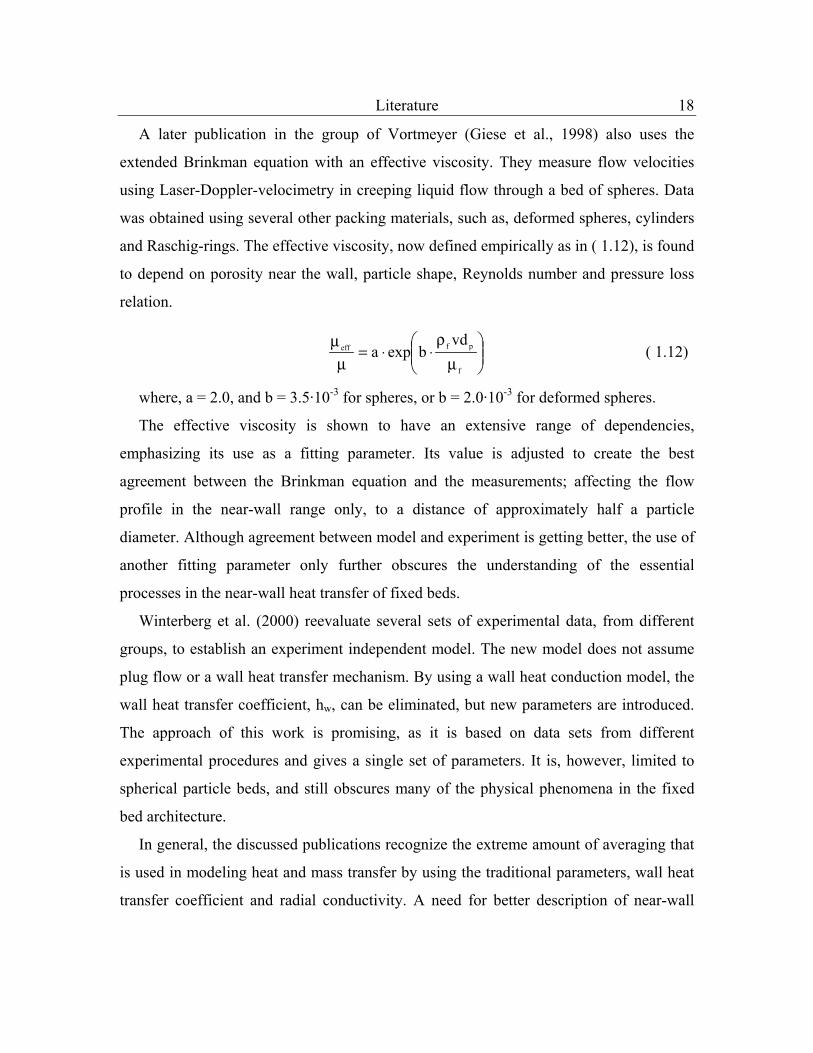
A later publication in the group of Vortmeyer (Giese et al., 1998) also uses the
extended Brinkman equation with an effective viscosity. They measure flow velocities
using Laser-Doppler-velocimetry in creeping liquid flow through a bed of spheres. Data
was obtained using several other packing materials, such as, deformed spheres, cylinders
and Raschig-rings. The effective viscosity, now defined empirically as in ( 1.12), is found
to depend on porosity near the wall, particle shape, Reynolds number and pressure loss
relation.
���
����
�
µρ
⋅⋅=µ
µ
f
pfeffvd
bexpa ( 1.12)
where, a = 2.0, and b = 3.5·10-3 for spheres, or b = 2.0·10-3 for deformed spheres.
The effective viscosity is shown to have an extensive range of dependencies,
emphasizing its use as a fitting parameter. Its value is adjusted to create the best
agreement between the Brinkman equation and the measurements; affecting the flow
profile in the near-wall range only, to a distance of approximately half a particle
diameter. Although agreement between model and experiment is getting better, the use of
another fitting parameter only further obscures the understanding of the essential
processes in the near-wall heat transfer of fixed beds.
Winterberg et al. (2000) reevaluate several sets of experimental data, from different
groups, to establish an experiment independent model. The new model does not assume
plug flow or a wall heat transfer mechanism. By using a wall heat conduction model, the
wall heat transfer coefficient, hw, can be eliminated, but new parameters are introduced.
The approach of this work is promising, as it is based on data sets from different
experimental procedures and gives a single set of parameters. It is, however, limited to
spherical particle beds, and still obscures many of the physical phenomena in the fixed
bed architecture.
In general, the discussed publications recognize the extreme amount of averaging that
is used in modeling heat and mass transfer by using the traditional parameters, wall heat
transfer coefficient and radial conductivity. A need for better description of near-wall
Page 37
Literature 19
transport processes to better understand these phenomena is identified. On the other hand
there is a strong drive towards simplification of the models for an uncomplicated
application in industrial use. Simple models using very general parameters, however,
tend to loose their grasp with physical phenomena and are very limited in their
applicability. The equipment and the process the parameters are determined on define the
limitations of the model. The parameters cannot be adjusted for physical changes since it
is not clear how these properties are included. For the sake of fundamental understanding
of the processes important in heat transfer in fixed beds, more emphasis has to be put on
the randomness of fixed beds and the flow and heat transfer patterns. By identifying the
essential features in the flow and heat transfer patterns parameters can be developed more
directly related to the physical phenomena. For industrial application it is essential that a
fixed bed model stays simple, but with more physical meaning in the parameters, a more
generally applicable model may be developed.
Essential in this new method would be to be able to visualize and identify the
characteristic phenomena in the fixed bed. The proposed method for this is
Computational Fluid Dynamics. CFD is still in a developmental stage for its use in fixed
bed modeling but shows much promise in its ability to show details in patterns that have
been impossible to measure with traditional techniques.
1.3.2 Earlier work done with CFD in fixed beds
CFD studies towards heat transfer and flow behavior in packed bed reactors have been
performed previously, over time CFD packages have become more sophisticated
allowing for more detailed simulations. Also the definition of what entails CFD has
changed over the years. In the earliest studies the one or two-dimensional pressure drop
equation over an averaged (homogenized) randomly packed bed was referred to as
computational fluid dynamics, as a dynamic fluid situation is described mathematically.
In later approaches, including this one, CFD refers to the use of a numerical method to
resolve a set of differential balances over a computational grid.
Page 38
Literature 20
The earliest fixed bed CFD simulations used two-dimensional models. Contrarily
Sørensen and Stewart (1974a, 1974b and 1974c) are one of the first groups to construct a
numerical iteration method for resolving flow and heat transfer in a three-dimensional
cubic array of spheres. The cubic array creates a predictable and repetitive structure
allowing for the full three-dimensional approach. The construction of the computational
grid is also discussed, the calculated flow is limited to creeping flow, and no turbulence
models were introduced. Dalman et al. (1986) investigated flow behavior in an
axisymmetric radial plane with 2 spheres; this limited the packing possibilities severely
but gave a first high-detail insight in flow patterns in fixed beds. This study showed that
eddies formed in between the spheres which led to a region of poor heat transfer. The
effect of Re and Pr numbers on this process were also investigated, and showed an
increasing problem with heat transfer as the Reynolds number increased. Lloyd and
Boehm (1994) did a very similar two-dimensional study; they used the commercial FE
package FIDAP and 8 instead of 2 spheres in line. In this study the influence of the
sphere spacing on the drag coefficients was investigated. It was also found that heat
transfer from the spheres decreased with decreased sphere spacing.
As computer capabilities are increasing the extent to which CFD can be applied to
complicated systems has increased considerably. Earlier studies in our group using a 3-
sphere model (Derkx and Dixon, 1996) were performed as one of the first models in 3D
simulation of fixed beds. This study focused on using CFD to obtain traditional modeling
parameters such as the Nuw numbers. An 8-sphere model followed (Logtenberg and
Dixon, 1998a; 1998b) the packing was modeled as two layers of four spheres, both layers
perpendicular to the flow in the tube with a tube-to-particle diameter ratio, N = 2.43.
Effective heat transfer parameters obtained from these CFD results matched theoretical
model predictions (Dixon and Creswell, 1979) reasonably well, but left room for
improvement. These studies were limited by the simplicity of the flow models used to
obtain data, e.g. the absence of contact points between the spheres and the wall and
amongst the spheres themselves. Another point for improvement in this model was the
small number of spheres, which may have resulted in less than realistic flow patterns.
Page 39
Literature 21
More recently, a 10-sphere model, N = 2.68, incorporating contact points between the
particles and between the particles and the wall (Logtenberg et al., 1999) was developed.
The 10-sphere model showed flow behavior and heat transfer behavior in such detail that
cannot be measured in standard experimental setups or described using conventional
packed bed models. By using three-dimensional models for these simulations the packing
need not be symmetrical (an implied feature in two-dimensional modeling), this way the
true nature of the wall effects are shown, as they would be present in a low-N tube.
Based on the modeling experience in these preliminary studies, and the capability to
increase model size as our computational capacity increased, a 44-sphere model was
created with N = 2 (Nijemeisland and Dixon, 2001). This specific geometry was used to
validate CFD results in fixed beds by comparing radial temperature profiles of the
simulations with experimental data in an identical setup. This work showed that with the
proper considerations of the limitations of the simulation and experimental setup taken
into account, both qualitative and quantitative agreement is established between CFD
simulation and experiments. Now that it is shown that CFD produces the same data as is
obtained experimentally, we can use the advantage of the CFD; where a lot more
information is available than is used for the comparison of CFD data with experimental
data, data that cannot be obtained through traditional experimental measurement.
Esterl et al. (1998) and Debus et al. (1998) applied a computational code by Nirschl et
al. (1995) to find flow profiles in an adapted chimera grid. This grid consists of a
structured grid, based on the flowing medium, which is overlaid by a separate structured
grid, based on the packing particles. Calculated pressure drops are compared against
predicted pressure drops using amongst others Ergun’s relation for a bed with an
identical porosity; the simulation data is in the same order of magnitude. Simulations
were performed in beds with up to 300 spheres. One of the aspects that may affect the
accuracy of the data in these simulations is that even though the bed, for which results
were discussed, consisted of 120 particles it is only approximately 5 layers deep,
resulting in a bed that mainly consists of inlet and outlet effects.
Page 40
Literature 22
Recently other research groups have used commercial CFD packages to simulate
behavior in fixed beds. Calis et al. (2001) applied the commercial code CFX-5.3 to a
structured packing of spheres. They used a model of a single stack of spheres from a
cubic structured packing. The simulation is performed over a repetitive section, a single
stack of spheres, out of a cubic array of spheres, similar to Sørensen and Stewart’s
packing. Several different types of structured packings are investigated, all based on
structured packing of spheres. The repetitive sections have varying N, from 1 to 4.
Values for pressure drop obtained from the simulations are validated against
experimental values. The used turbulence models (κ-ε and RSM) show similar results
with an average error from the experimental values of about 10%.
The Emig group at Erlangen is using a Lattice Boltzmann technique for simulation of
flow and simple reactions in a fixed bed of spheres. A dense packing of spheres in a
cylindrical column is created using a raining and compression algorithm. The created
packing topology is then divided in a cubic Lattice Boltzmann grid, where individual
elements are labeled as solid or fluid regions. A high resolution of the grid makes it
possible to obtain accurate flow profiles. Recently (Zeiser et al., 2002, Freund at al.,
2003) simple reactions have been added to the simulation, showing in bed species
profiles. The limitation of the Lattice Boltzmann technique is that it cannot handle energy
balances as of yet.
1.3.3 Other applications of CFD in fixed beds
Numerical modeling is also applied to other aspects of fixed beds. Modeling the flow
and heat transfer in a fixed bed may eventually be combined with these other areas to
create a full simulation of the fixed bed reactor concept.
Other areas of modeling include for example the research performed by the Bishop
group at the University of Kansas; they are simulating the reaction in fixed bed. The flow
in these simulations is approximated with a simple plug flow, the reaction, however, is
modeled from the distribution of the components in the gas phase and the fluid phase to
the reaction on the packing.
Page 41
Literature 23
In a fixed bed reactor, it is also possible to have multiple mobile phases. In our
simulations we limit the simulation to a single mobile phase, but in trickle bed or similar
reactors, there are two mobile phases in conjunction with a fixed bed.
At the Dudukovic group at the University of St. Louis, CFD is used for simulation of
trickle bed applications (Jiang et al., 2002a, 2002b). Two-phase flow is established in a
fixed bed topology; the bed in these simulations is modeled as a single porous structure.
It is seen as a single entity of which the porosity is defined at all the numerical elements,
the bed is not discretized; the solid phase is not explicitly defined. In this case, where an
entire, high N, fixed bed is simulated, a full discretization of the bed is still beyond the
possibilities of current computational capacities.
Page 42
24
1.4 Computational Fluid Dynamics
The application field for CFD as a modeling tool is constantly expanding, as
improvements in computer hardware, computational speed and memory size, as well as
improvements in software capabilities make CFD a feasible and accessible tool in a large
range of applications.
1.4.1 Introduction
The relatively young field of CFD is fast growing due to increasing computer
capabilities and a growing field of applications. It is an established research tool in
mechanical and civil engineering where it is used for stress calculations in solid
structures. It has also been used extensively in the automobile and airplane industry to
replace expensive wind tunnel testing of new designs. Recently the use of commercial
CFD packages has been introduced in the field of chemical engineering with the
introduction of specific fluid mixing programs and the option to solve for chemical
reactions (Bode, 1994; Harris et al., 1996; Ranade, 1995). In a review publication by
Kuipers and van Swaaij (1998) a very complete overview is given of the different areas
of chemical reaction engineering in which different aspects of CFD are applied. The CFD
that is discussed here focuses on very specific codes, dealing with the application of
different physical models to the CFD code to deal with the specific reaction engineering
problems. It is stated in this publication that for a wider use of commercial packages in
these problems, more physical models need to be included in the packages, which is
something we see today.
1.4.2 Theory
Solutions in finite volume CFD are obtained by numerically solving a number of
balances over a large number of control volumes or elements. The numerical solution is
Page 43
Computational Fluid Dynamics 25
obtained by supplying boundary conditions to the model boundaries and iteration of an
initially guessed solution.
The balances, dealing with fluid flow, are based on the Navier Stokes equations for
conservation of mass (continuity) and momentum. These equations are modified for each
case to solve a specific problem.
The complete collection of control volumes or elements, the mesh, is designed to fill a
large-scale geometry, described in a mesh file. The density of this mesh (the size of the
control volumes, a high mesh density is obtained by defining small control volumes) in
the overall geometry is determined by the user and affects the detail in the final solution.
Too coarse a mesh will result in an oversimplified flow profile, possibly obscuring
essential flow characteristics, or a non-converging iteration process. Too fine a mesh will
create a larger simulation geometry (more computational elements), which will require a
memory intensive computer system and increase iteration time.
After boundary conditions are set on the large-scale geometry the CFD code will
iterate the entire mesh using the balances and the boundary conditions to find a
converging numerical solution for the specific case.
1.4.2.1 Mesh topology
One of the most important parts of CFD modeling is the construction of the mesh
topology. The mesh establishes the accuracy of the simulation. It has to be chosen with
enough detail to describe the processes accurately and with a degree of coarseness that
enables solution within an acceptable amount of time. When an optimal density has been
found, refining the mesh will increase the model size without displaying more flow
detail. When it is coarsened the mesh may obscure, possibly essential, parts of the flow
detail. The mesh determines a large part of creating an acceptable simulation.
To determine an appropriate mesh density for the simulations several aspects were
taken into account. Previous studies towards CFD simulations of packed beds have been
performed within our research group (Derkx and Dixon, 1996; Logtenberg and Dixon,
1998a; 1998b; Logtenberg et al., 1999). In the earlier studies the mesh density was
Page 44
Computational Fluid Dynamics 26
investigated extensively. From experience from these previous studies an optimal mesh
density was chosen. Additional studies were done to find the optimal mesh density, for
the specific simulation geometries used here. This study focused mainly on maintaining a
3D topology that described the physical model accurately and was able to handle the flow
specifics of the packed bed geometry. Also, mesh densities were varied within the overall
grid to establish the optimal mesh density, describing the flow characteristics and
limiting the calculation times. More on the mesh generation application, GAMBIT, can
be found in paragraph 1.4.3.1 and specifics about the geometries used in this study can be
found in chapter 2 on model development.
1.4.2.2 Fluid flow fundamentals
For iteration CFD solvers use generalized fluid flow and energy balances based on the
Navier Stokes equations. The balances are generalized so the user can determine which
elements are included in the balance. The number of balances to be solved is also user
defined; it can be advantageous to not solve all balances initially.
The generalized balances that are used by the Fluent commercial CFD package are the
Navier Stokes equations for conservation of mass and momentum. Additional equations
are solved for heat transfer, species mixing or reaction or κ and ε for turbulent cases. The
basic equations and background of these balances are also stated in the Fluent UNS
user’s guide.
1.4.2.2.1 Navier Stokes equations
The general equation used for conservation of mass (the continuity equation) in the
Fluent UNS package, is defined as follows:
( )
mi
i Sxu
t=
∂ρ∂
+∂∂ρ ( 1.13)
The source term Sm contains the mass added through phase changes or user defined
sources. In general, and in the performed simulations, the source term was equal to zero.
Page 45
Computational Fluid Dynamics 27
The equation for conservation of momentum in direction i and in a non-accelerating
reference frame is given by:
( ) ( )ii
j
ij
ij
jii Fgxx
px
uutu +ρ+
∂∂τ
+∂∂−=
∂ρ∂
+∂ρ∂ ( 1.14)
In this balance p is the static pressure, τij is the stress tensor, ρgi is the gravitational
body force. Fi is an external body forces component; it can include forces from
interaction between phases, centrifugal forces, Coriolis forces and user-defined sources.
For the performed simulations it was zero.
The stress tensor τij for a Newtonian fluid is defined by:
ijl
l
i
j
j
iij x
u32
xu
xu
δ∂∂
µ−���
�
���
�
��
�
�
�
∂∂
+∂∂
µ=τ ( 1.15)
Here µ is the molecular viscosity; the second term on the right hand side of the
equation is the effect of volume dilation.
1.4.2.2.2 Turbulence models
All simulations were performed using a turbulent flow model. The flow may not be
turbulent in all control volumes of the simulation geometry, but if the turbulent
parameters are negligible the momentum equation reverts back to the laminar momentum
equation. In the cases where the turbulence is significant the parameters are then
available. The Renormalization Group (RNG) κ-ε model was used for the CFD
simulations. The RNG κ-ε model is derived from the instantaneous Navier-Stokes
equations using the Renormalization Group method as opposed to the standard κ-ε
model, which is based on Reynolds averaging. The major differences, in application,
from the standard κ-ε model (see Appendix 1: The standard κ-ε turbulence model) are
different empirical constants in the κ and ε balances and extra terms in the turbulent
dissipation balance (ε). The turbulence model still assumes that the flow is fully turbulent
and the effects of molecular viscosity are negligible. The Renormalization group methods
Page 46
Computational Fluid Dynamics 28
are a general methodology of model building based on the stepwise coarsening of a
problem. In the case of fluid dynamics, there are several coarsening steps. The initial step
goes from the original Newton’s equations for each molecule in a gas, to the kinetic
theory for dilute systems, using the Boltzmann’s equations for velocity and space-time.
An additional coarsening would describe a collection of atoms on a relatively large scale,
compared to mean free path distances and collision time, the Navier Stokes equations.
The main idea is that the RNG theory is applicable to scale-invariant phenomena that do
not have externally imposed characteristic length and time scales. In the case of
turbulence, the RNG theory is applicable to the small scale eddies, which are independent
of the larger scale phenomena that create them.
Several other turbulent models were available, the standard κ-ε model and a Reynolds
Stress Model, results for these different models were compared and it was shown there
were no significant differences in the results. The RNG κ-ε model was chosen because it
deals better with flow with high streamline curvature and high strain rates.
The RNG theory as applied to turbulence reduces the Reynolds number to an effective
Reynolds number (Reeff) by increasing an effective viscosity (µeff). Through this process
the small scale eddies are eliminated, which reduces computational demand considerably.
The new equation for the variation of the effective viscosity is
( ) ( ) ( )d
3/1
4d
43mol
moleff 4A31 ����� ≥�
�
���
�−
µε
+µ=µ ( 1.16)
where A is a constant derived by the RNG theory, ℓ is the eddy length scale and ℓd is
the Kolmogorov dissipation scale. So in this case when the eddy length scale is the
Kolmogorov scale, the effective viscosity is the molecular viscosity. This equation then
gives the interpolation formula for µeff(ℓ) between the molecular viscosity µmol valid at
dissipation scales and the high Reynolds number limit L>>ℓd.
Using the definition for the turbulent viscosity (µt = µeff - µmol), which gives a result
similar to the standard κ-ε model with only a small difference in the modeling constant,
Page 47
Computational Fluid Dynamics 29
the effective viscosity is now defined as a function of κ and ε in equation ( 1.16) in
algebraic form.
2
molmoleff
C1
���
�
���
�
εκ
µ+µ=µ µ ( 1.17)
The differential form of this equation is used in calculating the effective viscosity in
the RNG κ-ε model. This method allows varying the effective viscosity with the effective
Reynolds number to accurately extend the model to low-Reynolds-number and near-wall
flows.
The form of the main balances in the RNG κ-ε model are similar to the balances in the
standard κ-ε model, with the modification from the RNG statistical technique. The
momentum equation is now derived to be:
( ) ( )
���
�
���
�
��
�
�
�
∂∂
+∂∂
µ∂∂+
∂∂−=
∂ρ∂
+∂ρ∂
i
j
j
ieff
jij
jii
xu
xu
xxp
xuu
tu ( 1.18)
The effective viscosity in this balance is computed using the high-Reynolds-number
form. This is identical to the turbulent viscosity defined in the standard κ-ε model, the
only difference lies in the constant Cµ, it is 0.09 in the standard and 0.0845 in the RNG κ-
ε model.
ε
κρ=µ µ
2
t C ( 1.19)
When, however, low-Reynolds number effects need to be included the differential
form of equation ( 1.17) can be employed.
The transport equations for the turbulent kinetic energy, κ, and the turbulence
dissipation, ε, in the RNG κ-ε model are again defined similar to the standard κ-ε model,
now utilizing the effective viscosity defined through the RNG theory. Alternately a mean
strain rate, S, is used instead of the separate turbulence source terms.
Page 48
Computational Fluid Dynamics 30
( ) ( )ρε−µ+�
�
�
�
∂∂κµα
∂∂=
∂κρ∂
+∂ρκ∂
κ2
ti
effii
i Sxxx
ut
( 1.20)
and
( ) ( )RCSC
xxxu
t
2
22
t1i
effii
i −κερ−µ
κε+�
�
�
�
∂∂εµα
∂∂=
∂ερ∂
+∂ρε∂
εεε ( 1.21)
where ακ and αε are the inverse effective Prandtl numbers for κ and ε, respectively.
These variables are determined by the RNG theory through the analytically derived
formula,
eff
mol
3679.0
0
6321.0
0 3929.23929.2
3929.13929.1
µµ
=+α+α
−α−α ( 1.22)
where α0=1.0. In the high Reynolds number limit (µmol/µeff << 1), ακ = αε ≈ 1.393
S in equation ( 1.20) is the modulus of the mean rate-of-strain tensor, Sij, which is
defined as,
ijijSS2S = ( 1.23)
and R in equation ( 1.21) is given by
( )
κε
βη+ηη−ρη
= µ2
3
03
1/1C
R ( 1.24)
where η ≡ Sκ/ε, η0 ≈ 4.38, β = 0.012.
The model constants C1ε and C2ε from equation ( 1.21) are derived analytically
through the RNG theory and are respectively 1.42 and 1.68 (in the standard κ-ε model
these model constants are 1.44 and 1.92 respectively).
The major difference in the RNG κ-ε model from the standard κ-ε model can be found
in the ε balance where a new source term appears in the R term as described in ( 1.24).
This term is a function of both the turbulent kinetic energy, κ, and the turbulence
dissipation term, ε. The effect of the R term can be best illustrated when equation ( 1.21)
is slightly rewritten, so that the last two terms are combined:
Page 49
Computational Fluid Dynamics 31
( ) ( )κερ−µ
κε+�
�
���
�
∂∂εµα
∂∂=
∂ερ∂
+∂ρε∂
εεε
2*2
2t1
ieff
ii
i CSCxxx
ut
( 1.25)
where C*2ε is given by,
( )
3
03
2*2 1
/1CCC
βη+ηη−η
+= µεε ( 1.26)
We can now see the contribution of this factor as a function of the strain rate, η. In
areas where η < η0 (where η0 ≈ 4.38, as mentioned before), the R term makes a positive
contribution and C*2ε becomes larger than 1.68. When we look, for example, in the
logarithmic layer, where η ≈ 3.0, it results in a C*2ε ≈ 2.0, which is close to the value of
C2ε for the standard κ-ε model, 1.92. We conclude that for moderately strained flows the
RNG model gives results comparable to the standard κ-ε model.
Alternatively, in areas of high strain rate, η > η0, the R term makes a negative
contribution, reducing the value of C*2ε to less than C2ε. This means that compared to the
standard κ-ε model the RNG model has a smaller reduction of ε, augmenting the value of
ε resulting in a reduced κ and eventually the effective viscosity. The RNG model now
yields a lower turbulent viscosity in the high strain flows than the standard κ-ε model.
The R term in the RNG κ-ε model makes the turbulence in this model sensitive to the
mean rate of strain. This results in a model that is responsive to effects of strain and
streamline curvature, a feature that is non-existent in the standard κ-ε model. The
inclusion of this effect makes the RNG κ-ε model more suitable for complex flows.
1.4.2.2.3 Energy equations
The RNG model provides its own energy balance, which is based on the energy
balance of the standard κ-ε model with similar changes as were seen in the κ and ε
balances. The energy balances for the standard κ-ε model are described in Appendix 1:
The standard κ-ε turbulence model. The RNG κ-ε model energy balance is defined as a
transport equation for enthalpy,
Page 50
Computational Fluid Dynamics 32
( ) ( ) ( ) hk
ieffik
ieffp
ii
i Sxu
DtDp
xTc
xxhu
th +
∂∂
τ++���
����
�
∂∂µα
∂∂=
∂ρ∂
+∂ρ∂ ( 1.27)
where h is the sensible enthalpy, τik is the deviatoric stress tensor and α is the inverse
Prandtl number for temperature. There are four contributions to the total change in
enthalpy, the temperature gradient, the total pressure differential, the internal stress and
the source term, including contributions from reaction etc. The RNG model gives an
implicit formula for α in terms of the ratio of molecular and effective viscosities,
µmol/µeff, as
eff
mol
3679.0
mol
6321.0
mol 3929.23929.2
3929.13929.1
µµ
=+α
+α−α
−α ( 1.28)
which is similar to equation ( 1.22), using αmol instead of α0, αmol ≡ 1/Pr = kf/µcp. In
the traditional turbulent heat transfer model, the Prandtl number is fixed and user defined,
the RNG model treats it as a variable dependent on the turbulent viscosity. It was found
experimentally that the turbulent Prandtl number is indeed a function of the molecular
Prandtl number and the viscosity (Kays, 1994).
1.4.2.2.4 Wall functions
To be able to resolve the flow solution near solid surfaces with zero flow boundary
conditions, there needs to be some special conditions set. Besides the zero flow
boundaries, the presence of a solid surface also affects the turbulence; the dissipation of
turbulent kinetic energy is much larger near a solid surface since the turbulence is
damped. Slightly further away from the solid surface, still in the wall boundary layer,
there is a source of turbulent kinetic energy due to the local Reynolds stresses and the
large gradient of the mean velocity. Several methods are available to resolve both the
zero flow condition at the solid surface and the turbulent conditions near the solid
surface.
The simplest solution is also the most computationally intensive one. At the zero flow
boundary a strong gradient develops for a number of variables in the simulation, to
Page 51
Computational Fluid Dynamics 33
directly resolve these gradients with a single model one could adapt the mesh
appropriately. This would entail greatly increasing the mesh density near all solid
surfaces. This solution is undesirable in the proposed study as there are numerous solid
surface regions in the fixed bed geometry. Resolving the zero-flow boundary in this way
would mean increasing the mesh size to proportions that would not be solvable on the
available computational equipment.
The Fluent CFD code does offer alternate solutions to resolving the solid surface
boundary, as this is a very common feature. The alternative to resolving the gradients at
the solid surface completely is imposing a wall function that models these gradients in
the single layer of mesh adjacent to the solid surface boundary. There are several
different wall-functions available to deal with this gradient.
The general goal of the wall functions is to replace the direct modeling of the viscous
sublayer and the transition region to the fully turbulent layer with one empirical model, in
effect linking the solution variables in the cells near the solid surface to the
corresponding values on the solid surface. In our simulations we have employed two
different wall function models, the standard wall function and the non-equilibrium wall
function.
The standard wall function is based on a proposal in a publication by Launder and
Spalding (1974) and it has been used widely for industrial flows. The wall function
describes the velocities, temperatures and turbulent quantities in the application area.
( )** Eylnk1U = ( 1.29)
where,
ρτκ
≡ µ
w
5.0P
25.0P* CU
U ( 1.30)
µκρ
≡ µ P5.0
P25.0
* yCy ( 1.31)
Page 52
Computational Fluid Dynamics 34
in equation ( 1.29),
k = von Karman’s constant (= 0.42)
E = empirical constant (= 9.81)
in equation ( 1.30),
UP = mean velocity at P
κP = turbulent kinetic energy at P
Cµ = model constant used in defining the turbulent viscosity (equation ( 1.19))
τw/ρ = related to friction velocity, ρτ≡τ wu
in equation ( 1.31),
yP = distance of point P to the wall
Relation ( 1.29) is used to determine the mean velocity of a control volume when
y*>11.225. When y*<11.225 the laminar stress strain relationship is applied:
** yU = ( 1.32)
To describe boundary layer flow a commonly used parameter is y+, which is defined
as µρ≡ τ+ yuy . This parameter is used to subdivide the area near the zero flow
boundary based on the actual distance from the wall, modified by the friction velocity, uτ,
and the fluid viscosity. Fluent uses y*, instead of y+, in modeling the behavior near the
wall, which is a similar parameter.
For the thermal conditions another parameter determines whether a linear or
logarithmic relation is used to calculate the profile over the control volumes. The thermal
conduction layer is different from the viscous sublayer, it is dependent on the fluid. The
method is conditional depending whether a control volume is within the thermal sublayer
or not. The cut-off is determined by the parameter *Ty . The value of this parameter is
determined by where the linear and logarithmic areas intersect and is calculated using the
fluid molecular Prandtl number.
Page 53
Computational Fluid Dynamics 35
( )
"qkCTT
T5.0
P25.0
Pw*
�
µρ−≡
2P"q
kC21* UPryPr
5.0P
25.0
�
µρ+= ( )*T
* yy < ( 1.33)
( )[ ] ( ){ }2ct
2Pt"q
kC21*1
t UPrPrUPrPrPEylnPr5.0
P25.0
−+ρ++= µ
κ � ( )*
T* yy >
where P is computed using (Launder and Spalding, 1974),
( )24.0
t
t
5.0
PrPr
1PrPrA
4sin4P �
�
���
����
����
�−�
�
���
�
κππ= ( 1.34)
where,
TP =temperature at the cell adjacent to the wall
Tw = temperature at the wall
Prt = turbulent Prandtl number (0.85 at the wall)
A = Van Driest constant (=26)
κ = von Karman’s constant (=0.42)
E = wall function constant (=9.793)
Uc = mean velocity magnitude at *T
* yy =
Now the thermal sublayer thickness, *Ty , is determined when the fluid conditions are
known from the molecular Prandtl number and the intersection of the linear and
logarithmic regions.
From the relations in equation ( 1.33), depending on the y* value of the cell adjacent to
the wall, the wall temperature, Tw, and the heat flux, "q� , are related; so one can be
calculated from the other depending on whether a constant heat flux or constant wall
temperature has been set on the wall.
The standard wall function works well for a broad range of near wall flow conditions.
However, when the modeling conditions deviate too much from the assumptions, the
model becomes less reliable. Especially the constant shear stress and the local
Page 54
Computational Fluid Dynamics 36
equilibrium assumptions restrict the universality of the standard wall functions. The local
equilibrium assumption states that the turbulence kinetic energy production and
dissipation are equal in the wall bounded control volumes. In cases where there is a
strong pressure gradient near the wall (increased shear stress) or the flow does not satisfy
the local equilibrium condition an alternate model, the non-equilibrium model, is
recommended.
The non-equilibrium wall function is more suitable for complex flows involving
separation, reattachment, and impingement where the mean flow and turbulence are
subjected to severe pressure gradients and change rapidly. In such flows, improvements
can be obtained, particularly in the prediction of wall shear and heat transfer.
The higher sensitivity to pressure gradient in the non-equilibrium wall model is
expressed in the definition of the velocity in equation ( 1.29) effectively replacing the
definition in equation ( 1.30) with:
U~kC
Uw
5.025.0* ⋅
ρτ≡ µ ( 1.35)
��
���
�
µ+
ρκ−
+���
�
�
ρκ−=
2v
5.0*v
v5.0*
v ykyy
yyln
ky
dxdp
21UU~ ( 1.36)
where,
*v5.0
p25.0v y
kCy ⋅
ρµ≡
µ
and 225.11y*v =
In the non-equilibrium wall function the heat transfer procedure remains exactly the
same. The mean velocity is made more sensitive to pressure gradient effects. This does
not seem to be much of an issue in our simulations.
1.4.2.3 Numerical solutions
The governing partial differential equations for the conservation of momentum and
scalars such as mass, energy and turbulence are solved in the integral form. Fluent UNS
uses a control-volume based technique, which consists of three basic steps.
Page 55
Computational Fluid Dynamics 37
• Division of the domain into discrete control volumes using the computational grid.
• Integration of the governing equations on the control volumes to create an algebraic
equation for unknowns such as pressure, velocity and scalars.
• Solution of the discretized equations.
The governing equations are solved sequentially. The fact that these equations are
coupled makes it necessary to perform several iterations of the solution loop before
convergence can be reached. The solution loop consists of 7 steps that are performed in
order.
1. The momentum equation for each direction is solved using the current pressure
values (initially the boundary condition is used), in order to update the velocity field.
2. The obtained velocities may not satisfy the continuity equation locally. Using the
continuity equation and the linearized momentum equation a ‘Poisson-type’ equation
for pressure correction is derived. Using this pressure correction the pressure and
velocities are corrected to satisfy continuity.
3. and ε equations are solved with corrected velocity field.
4. All other equations (e.g. energy, species conservation etc.) are solved using the
corrected values of the variables.
5. Fluid properties are updated
6. Any additional inter-phase source terms are updated.
7. A check for convergence is performed. If convergence is not reached to within the
specified tolerance, the process is repeated from step 1.
1.4.3 CFD solver and additional programs
To be able to conduct our CFD simulations we used a commercially available code,
Fluent UNS. This code is written by Fluent Inc. and uses unstructured meshes. The CFD
package consists of two different modules in which different parts of the process take
place.
Page 56
Computational Fluid Dynamics 38
a b
Figure 1.1. typical examples of a) the surface mesh on a number of spheres and a
section of the cylinder and b) a section of the interior mesh in a plane indicated in part a.
The first step, mesh creation, is done with GAMBIT. The GAMBIT meshing program
is multifunctional; it can create both 2 dimensional and 3 dimensional simulation
geometries. The entire mesh creation is performed in GAMBIT, from the initial
geometric design to labeling all volumes and surfaces that build up the final simulation
model. The 3D meshes used in this work (see Figure 1.1b) are imported in Fluent UNS to
impose boundary conditions, iterate and post-process the data.
1.4.3.1 Mesh creation with GAMBIT
As was stated before, the creation of the mesh is the most important step in CFD. The
mesh density, or inversely, the size of the control volumes, determines the accuracy of
the simulation. The mesh consists of four major concepts, volumes, surfaces, edges and
nodes. These concepts are hierarchical, a volume is bounded by surfaces, a surface is
bounded by edges and an edge consists of nodes.
The mesh creation in GAMBIT consists of three major steps. In the first step the
geometry of the model is established, a CAD program is used to determine dimensions.
The second step is the creation of the surface mesh, which is placed on the surfaces
created in the CAD geometry modeling phase. The final step is the interpolation of the
surface mesh to the final fully three-dimensional volume mesh.
Page 57
Computational Fluid Dynamics 39
1.4.3.1.1 CAD geometry design
The topology of the simulation model is established in the initial CAD geometry
design phase. In this initial phase the major solid and fluid region interfaces are
established. The GAMBIT program uses a top-down design system. This means that the
overall geometry is defined starting with the major volumetric parts; interfaces and
specific points are created in a later stage. This method is relatively fast, especially when
the simulation geometry consists of simple geometric features. When, however, more
detail is required in the mesh of the model the top-down design has no specific
advantages over the bottom-up method. The bottom-up method starts with defining nodes
and building up to edges, surfaces and eventually volumes. In the bottom-up method
more advance planning on the construction of the model and the mesh is required.
When a model is created with a top-down, or constructive solid geometry (CSG)
method the interstitial space, such as our fluid region, has to be specifically defined. First,
an overall geometry is defined, e.g. the tube containing the particles. Second, the particles
are placed in the tube at their appropriate locations. To create the proper fluid region the
particle volumes need to be subtracted from the tube volume. After creating the
appropriate fluid and solid regions, the region interfaces need to be linked. When the
fluid region is created it is a separate region from the solid particles, and the surfaces
bounding the particles need to be linked to the surfaces bounding the fluid region. The
linking of these interface surfaces is essential in creating an appropriate energy solution
in the model.
When all regions and their interfaces have been properly defined the simulation model
can be meshed.
1.4.3.1.2 Mesh creation
Depending on the detail of mesh refinement required the simulation geometry can be
meshed at three different levels, edges, surfaces and volumes. When a global uniform
mesh suffices the meshing can take place on the volume level. At this point one uniform
Page 58
Computational Fluid Dynamics 40
control volume size is determined and the entire simulation geometry is meshed with this
standard control volume size, creating a uniform mesh density.
Figure 1.2, edge mesh, showing the graded node spacing, and the resultant surface
mesh in a selection of the ws-995 geometry.
When local refinement is required, i.e. in sensitive regions of the geometry, different
mesh densities can be defined to surfaces or edges specifically. For example near contact
point areas, between particles in the geometry, or between particles and the externally
bounding column wall, the mesh needs to be finer than in larger void areas in the
geometry to be able to get a converging flow solution. To be able to adjust the mesh
locally mesh densities have to be defined on edges along these contact points, see Figure
1.2 through Figure 1.4.
When defining a refinement in the mesh along a single edge several schemes are
available. Node distribution on the edge can be uniform or graded with a higher node
density in the appropriate areas.
When a mesh with the proper mesh densities has been created it is exported to a
format that can be imported in Fluent UNS, the CFD solver. Before export the surfaces
and solid regions are labeled so they can be easily identified in the solver. At this point it
is also possible to group a series of surfaces, or volumes, together so as to more easily
define similar boundary conditions for a group of entities.
Page 59
Computational Fluid Dynamics 41
Figure 1.3, selected control volumes in the ws-995 mesh interpolated from the node
spacing and surface mesh shown in Figure 1.2.
Figure 1.4, two-dimensional display and a detail of the control volumes in the fluid
region of the ws-995 mesh showing the size grading.
1.4.3.1.3 Mesh specifics in fixed bed modeling
For all types of geometries the creation of the mesh has different obstacles. In the
meshing of a fixed bed geometry the major issue is resolving the areas where two solid
surfaces touch, the contact points. As was discussed in the validation study (Nijemeisland
and Dixon, 2001) it is not possible to incorporate actual contact points of the spheres with
Page 60
Computational Fluid Dynamics 42
each other or the wall when turbulent flow needs to be resolved. By having two solid
faces touch in a flow geometry, certain control volumes in the fluid zone that are located
near the contact point are created with infinitely small edges, resulting in an irresolvable
simulation condition. In the validation geometry this problem was resolved by reducing
the size of the spheres to 99% of their original size, small gaps were created between the
contacting solid surfaces so fluid-zone control volumes with a finite size could be placed
near the contact points. It was shown that with the simulation condition in the validation
model the no-flow zone near the contact points was retained and the influence of the
small gaps was negligible to the flow solution.
A similar process was used in the creation of the N = 4 wall-segment model. To
accommodate the more extreme steam reforming simulation conditions, higher pressure
and higher flow rates, it was necessary to reevaluate the appropriate amount of particle
size reduction. To create a mesh that would give a flow solution similar to a geometry
with touching particles an investigation was performed to find the influence of the gap
size at high Reynolds numbers (Rep = 35000). It was found that at these high flow rates a
99% reduction of the spheres would result in considerable amounts of flow in the gaps,
creating an unrealistic flow field. The gap size was reduced until the no-flow area around
the contact point was reestablished. The resulting particle size reduction was 99.5% and
the meshing results can be seen in Figure 1.2 through Figure 1.4.
1.4.3.2 Solving the CFD problem with Fluent UNS
When a mesh is completed with its grid density and all other complications resolved,
the actual computational part of the CFD can be started. At this point the completed
geometry can be imported into the solver and the CFD simulation is started.
Again a series of steps are to be performed; first, the boundary conditions on the
system need to be set, next the process iteration parameters need to be set. With the
boundary conditions defined the simulation can be performed. The final step in obtaining
the desired data is the post-processing of the data in which the desired data sets are taken
from the simulation data.
Page 61
Computational Fluid Dynamics 43
1.4.3.2.1 Imposing boundary conditions
The boundary conditions determine the flow and thermal variables on the boundaries
of the physical model. There are a number of classifications of boundary conditions:
• Flow inlet and exit boundaries: pressure inlet, velocity inlet, inlet vent, intake fan,
pressure outlet, outflow, outlet fan, exhaust fan.
• Wall, repeating, and pole boundaries: wall, symmetry, periodic, axis
• Internal cell zones: fluid, solid
• Internal face boundaries: fan, radiator, porous jump, wall, interior
In our model we use either translational periodic flow boundaries at both the flow inlet
and flow outlet of the column, or a velocity inlet at the flow inlet of the column and a
pressure outlet at the flow exit boundary. To create a flow solution the translational
periodic boundaries are used, and the overall flow is defined as a total mass flux through
the boundary. By imposing the translational periodic boundaries a generic developed
flow solution is obtained. Since the translational periodic boundary defines the column
inlet to be identical to the column outlet, there is no flow development in the bed; a
steady state flow situation is obtained. The periodic boundaries remove the effects of an
entrance or exit effect in the bed. It is generally accepted that when flow enters a
structured or randomly packed fixed bed, an area near the entrance of the bed has an
undeveloped flow profile as the fluid is adjusting from one flow environment to another.
A similar situation is found near the exit of the bed, where a sudden change in pressure
drop is experienced and the flow ‘relaxes’ before it actually exits the bed. By imposing
the periodic boundaries, the effects of the inlet and exit are completely negated. The
overall size of the model can now be greatly reduced. In a full model in which an actual
bed inlet and outlet are modeled a large portion of bed needs to be modeled just to
eliminate entrance and exit effects in a central portion of the bed.
When the energy balances are solved the flow inlet and exit boundaries are set as a
velocity inlet and a pressure outlet, but the flow parameters in these boundary conditions
are not used at this point. To solve a steady state temperature profile in a generic section
Page 62
Computational Fluid Dynamics 44
of the bed it is necessary to remove the periodic boundary conditions on the inlet and
outlet. With periodic boundary conditions on the column and a heat flux through the
column wall, the steady state solution will be a uniform temperature in the bed at the wall
temperature. Since we want to investigate the energy penetration into the bed from the
wall, it is necessary to reinstate the generic bed section as a section in a larger bed,
defining different inlet and outlet conditions. To calculate the development of the
temperature profile into the bed a series of simulations have to be performed. In the series
of simulations the generic sections are virtually stacked by imposing the outlet
temperature conditions of one section as the inlet conditions of the downstream section.
The column and packing exterior are defined as wall boundaries. The wall boundaries
separate the fluid zone, in between the particles, from the solid zones, inside the particles;
they also constrain the fluid zone to within the column. Internal face boundaries are not
used in our model.
Additional to the boundary conditions at the physical boundaries a beginning
condition, or initial guess has to be established. This initial guess can be seen as similar
to a time initial condition. To create a fast steady state solution it helps to have an initial
guess relatively close to the final solution. In our simulations the initial guess for the flow
conditions was set to a constant axial flow of the superficial velocity based on the
simulations Reynolds number. The initial guess for the temperature solution was a
uniform temperature at the inlet gas temperature, both in the fluid and solid regions. For
staged solutions, the solution set of the upstream solution is used as an initial guess for
the next downstream section, as it is expected that the change through the column is
gradual and small between subsequent steps.
With the determination of the boundary conditions the physical model has been
defined and a numerical solution can be provided. It is now necessary to determine how
the solution will be established by setting the iteration parameters.
Page 63
Computational Fluid Dynamics 45
1.4.3.2.2 Setting iteration parameters
There are two main iteration parameters to be set before commencing with the
simulation. The underrelaxation factor determines the solution adjustment after each
iteration step; the residual cut off value determines when the iteration process can be
terminated.
The relaxation factor is the factor with which the iteration step change is multiplied
before it is applied to the result for the next iteration step. When this factor is larger than
1 (one) the process is called over-relaxed. In an over-relaxed process the step change is
large and convergence should be reached faster. It is, however, not recommended to over
relax a process unless it is very stable. In a less stable or particularly nonlinear system,
for example in some turbulent flow or high-Rayleigh-number natural-convection cases,
over-relaxation may lead to divergence of the process. When the relaxation factor is less
than 1 (one) the process is called under-relaxed. When under-relaxed the iteration process
is slower, since the step change is small, but less likely to diverge.
The second parameter, the residual value, determines when a solution is converged.
The residual value (a difference between the current and the former iteration value) is
taken as a measure for convergence. In an infinite precision process the residuals will go
to zero as the process converges. On practical computers the residuals decay to a certain
small value (‘round-off’) and then stop changing. This decay may be up to six orders of
magnitude for single precision computations. By setting the upper limit of the residual
values the ‘cut-off’ value for convergence is set. When the set value is reached the
process is considered to have reached its ‘round-off’ value and the iteration process is
stopped.
Besides adjusting these two major parameters there are other tricks to have a
simulation converge. When convergence of, for example, turbulence elements in the flow
balances or energy balances is problematic, using the flow solution as an initial guess can
be helpful. To do this, first only the velocity elements in the balances are iterated, the
result of this initial run is then used as a starting point for the iteration of the complete
Page 64
Computational Fluid Dynamics 46
balances. In this way the initial guess for the final solution is better and will help in
getting a simulation to converge.
1.4.3.2.3 Post-processing the simulation data
When the simulation has converged the last data set is stored as a final solution. This
data set has a record of the status of all elements in the model, temperature, densities,
pressures, flow aspects etc. To be able to interpret the data it needs to be ordered and
reduced to comprehensible sizes. This displaying of the data is called post-processing and
makes it possible to compare the different simulations with each other and with external
data.
There are as many ways of displaying the data as there are data points so it is
important to select the data representation that is required for the desired data
comparison. Some of the standard visualization options available are contour plots and
velocity vector plots.
Contour plots will give a plot in a defined collection of control volumes, which can be
a plane or a volume, of contours of another variable. For example a plane can be defined
as a constant x-coordinate plane (y-z plane), we can then make a contour plot showing
temperature contours in this plane. In the same plane a velocity contour plot can be made
showing absolute velocities of the fluid in the defined plane. Other variables that can be
used for contour plots are, magnitude of velocity components, turbulence components,
local pressure etc.
Velocity vector plots can be made to get an insight into the flow patterns in the overall
geometry or detailed at specific locations. The density and magnification of the velocity
vectors in the specified field can be manually changed to get a most optimal picture. The
field density has a maximum limitation, the amount of elements in the model. Figure 1.5
shows the velocity vector plot that corresponds with the mesh shown in Figure 1.1b.
Besides these qualitative data export methods it is also possible to export the
numerical data in many different forms. Direct export of selected data sets is facilitated
Page 65
Computational Fluid Dynamics 47
for a number of external applications; also it is possible to export data in ASCII format
for further manipulation.
Another method for exporting the numerical data is the two-dimensional plot function
in which two data sets can be plotted against each other. This function is useful when for
example radial velocity or temperature profiles need to be compared. From different
simulations identical plots can be created and a direct comparison of the numerical data is
possible.
Figure 1.5. velocity vector plot as obtained from Fluent UNS, vectors colored by axial
velocity component [m/s].
Page 66
48
1.5 Validation
Since the CFD methodology is not specifically designed for application in constrained
geometries, such as particle packed beds, it is necessary to verify if the simulated results
are valid. Although the CFD code is based on fundamental principles of flow and heat
transfer some of the boundary issues are modeled using empirical data not necessarily
appropriate for the fixed bed application. In this chapter a previously performed
validation study is presented to validate the used CFD code and the used boundary
models for use in particle packed fixed beds.
In this paragraph our intent is to show that a validation of CFD in fixed bed
geometries was performed. A short description of the experimental and simulation
methods will be given as well as a description of the setup and models used. Additionally
some of the results and discussion will be presented. For a concise description of the
study please refer to the publication of the work, Nijemeisland and Dixon, 2001. For a
more complete description of the work refer to the thesis work, Nijemeisland, 2000.
1.5.1 Experimental method and data
The experimental setup used is a single tube, heated wall, packed bed setup as is
shown in Figure 1.6. The packed bed consisted of 44 spheres with a diameter of one inch.
The column (single tube) in which they were packed has an inner diameter of two inches.
The column consists of two main parts. The bottom part is a nylon tube, 6 inches in
length that was not directly heated; this part is the calming section, where a steady flow
profile in the bed was established. The second part of the column is the heated section.
This section is heated with steam flowing in between its double wall and was maintained
at a constant temperature. The 44-sphere packed bed fills the entire calming section and
part of the heated section leaving room after the packing for installation of the
thermocouple cross for measuring gas temperatures above the bed. The temperature of
Page 67
Validation 49
the air is measured at the column inlet. After the bed a radial temperature profile is
measured using a thermocouple-cross, depicted in Figure 1.6. The thermocouple-cross is
inserted in the column approximately 5 mm above the top layer of the bed to measure the
radial temperature profile in the gas flow. All thermocouples were K type thermocouples.
thermocouple cross
insulation
heated wall
packing
steam in
rotameter
dryer
air in
steam out
TC
P
P
r/r = 0.30r/r = 0.56r/r = 0.80
r/r = 0.91r/r = 0.70r/r = 0.46
ttt
ttt
Figure 1.6, experimental setup and detail of the thermocouple cross, with the radial
positions of the thermocouples indicated, used for temperature data collection.
A radial temperature measurement consists of establishing and recording a steady state
temperature profile for a combination of a specific bed length, Reynolds number and
angle of thermocouple cross. A total of four thermocouple-cross positions are used for a
measurement by rotating the cross 15, 30 and 45-degrees from the initial orientation. By
rotating the thermocouple cross a good spread of data points covering the entire radial
plane is ensured, giving a full picture of the angular spread of the radial temperature
profile. Particle Reynolds numbers were varied from 373 to 1922 at approximately 100
units intervals, bed lengths were varied from 0.132 through 0.42 m by two packing layers
increments.
Page 68
Validation 50
Radial temperature profiles in the bed are established by plotting the collected data
dimensionless temperature vs. dimensionless radial position. Figure 1.7 shows some of
the temperature profiles acquired with the experimental method.
0
0.2
0.4
0.6
0.8
1
0 0.2 0.4 0.6 0.8 1r/rt
θθθθ
experimental dataexperimental fit
a0
0.2
0.4
0.6
0.8
1
0 0.2 0.4 0.6 0.8 1r/rt
θθθθ
z=0.420z=0.384z=0.348z=0.312z=0.276z=0.240z=0.204z=0.168
b
Figure 1.7, a) measured and fitted radial temperature profile at z = 0.42 and Rep = 879,
and b) averaged radial temperature profiles at a series of bed lengths at Rep = 986.
Figure 1.7a shows the complete dataset from the measurement at a full bed length and
Rep = 879, included is a fit to the data. It can be seen that as we move further towards the
wall the spread in the temperature increases. The large spread is due to the different
conditions at which measurements were taken as the thermocouple is rotated. The data is
reduced from a two-dimensional temperature field (radial and angular coordinates) to a
one-dimensional field by angular averaging. Figure 1.7b shows the development of the
radial temperature profile in the bed, as a series of temperature profiles at different bed
lengths are displayed. The figure is a composite of as many different measurements as
there are profiles shown. To be able to take a radial temperature profile measurement at
an alternate bed length in the experimental setup, the system has to be shut down, the bed
has to be adjusted and the thermocouple cross has to be repositioned.
Page 69
Validation 51
1.5.2 CFD model and data
For the validation study a CFD geometry was created with the same dimensions as the
experimental setup. The CFD geometry was limited to the tube containing the packed bed
of spheres. The bed of spheres in the CFD geometry consisted of 22 layers of 2 spheres,
identical to the longest bed (z = 0.42 m) used in the experimental setup. The layout of the
geometry is shown in Figure 1.8.
a b
Figure 1.8, the layout of the CFD geometry of an N = 2 bed, used for the validation
study; a) shows the bottom section of the bed, b) shows the top view of the bed.
Simulations were performed using the same boundary conditions as were encountered
in the experimental measurement, to be able to directly compare the acquired temperature
profiles. Data extraction from the CFD simulation is relatively easy. A plane is defined at
the axial position where in the experimental measurement the thermocouple cross was
located, this way similar temperature profiles are collected. In the CFD data set the exact
locations of the temperature ‘measurements’ are known, but to create a comparable
representation, the data is also reduced to a one-dimensional radial temperature profile.
Page 70
Validation 52
0
0.2
0.4
0.6
0.8
1
0 0.2 0.4 0.6 0.8 1r/rt
θθθθ
a0
0.2
0.4
0.6
0.8
1
0 0.2 0.4 0.6 0.8 1r/rt
θθθθ
z = 0.420z = 0.348z = 0.276
b
Figure 1.9, radial temperature profiles acquired by CFD simulation for a) z = 0.42 and
Rep = 1922, and b) a series of axial positions at Rep = 986.
Figure 1.9a shows the radial temperature profile at z = 0.42 for the run at Rep = 1922.
Similarly to the temperature profile shown in Figure 1.7a we see that there is a
considerable spread in the temperature data along the radius of the column. The CFD
temperature profile does give a more continuous profile, as data is available at many
more radial positions than was the case for the experimental measurement. Figure 1.9b
shows, similarly to Figure 1.7b, a series of temperature profiles at Rep = 986 for different
axial positions. The difference being that the CFD profiles were acquired by simply
collecting the data at a different axial position in the same geometry. From Figure 1.9b
we see that the shape of the profiles at lower axial positions is noticeably different from
the profile at the bed end. Since in the CFD data set the bed was not removed to measure
at a shorter bed, the measurements at lower axial position are actual temperature profiles
in the bed. The fact that the profiles at the end of the bed differ qualitatively from the
profiles in the bed is caused by the fact that temperature data is collected only in the fluid
region. In the bed the fluid region is smaller, due to the presence of the packing particles.
The different domain from which data is collected combined with the different flow
profiles in and outside the bed, see Figure 1.10, results in the different temperature
profiles.
Page 71
Validation 53
0
1
2
3
4
5
0 0.2 0.4 0.6 0.8 1r/rt
v/vin z = 0.204z = 0.384z = 0.420
Figure 1.10, radial velocity profiles at different axial locations, Re = 1922.
The different profiles in different regions of the bed have two consequences. First,
comparisons between CFD data and experimental data could not be made at different
axial positions as the temperature profiles differ qualitatively. Secondly, the general
assumption that a measured radial temperature profile just downstream of the bed will be
the same as a temperature profile in the bed will have to be reconsidered. At most a
profile measured downstream of the bed will have similarities to the temperature profiles
in the bed.
It does need to be pointed out that differences, in velocity and temperature profiles, in
and downstream of the bed are exacerbated due to the N = 2 geometry. The sizes of the
particles and the voids are relatively large for the lower N cases, resulting in an increased
difference between the profiles. For larger N the differences may be less.
1.5.3 Comparing experimental and CFD data
The radial temperature profiles obtained in the experimental setup and in the CFD
simulations were directly compared. The comparisons showed that experimental
temperature profiles and CFD produced profiles are qualitatively and quantitatively
Page 72
Validation 54
comparable. Although several adjustments to the final temperature profiles of both the
experimental results and the CFD simulation were needed to compensate for deviations
in the measurements and simulations. Factors that were adjusted include thermal
conduction through the thermocouple cross for the experimental results and radiation
effects and solid-solid conduction that were neglected in the CFD simulations.
0
0.2
0.4
0.6
0.8
1
0 0.2 0.4 0.6 0.8 1r/rt
θθθθ
CFD dataexperimental data
a 0
0.2
0.4
0.6
0.8
1
0 0.2 0.4 0.6 0.8 1r/rt
θθθθ
CFD dataexperimental
b
Figure 1.11, direct comparisons of experimental and CFD temperature profiles at
z = 0.42 for a) Rep = 986, and b) Rep = 1922.
The direct comparison of the temperature profiles acquired experimentally and from
the CFD simulation, shown in Figure 1.11, illustrates the favorable qualitative and
quantitative comparison between the two different methods. We have shown, through
comparison of radial temperature profiles, that when CFD is applied to fixed bed analysis
it gives identical, though more detailed, results compared to experimental data
acquisition. CFD can be considered a new method of data acquisition in fixed beds. This
new method requires a considerable amount of work to set up, but once operational
provides a wealth of data unavailable through any other method.
Page 73
55
2. Simulation Geometry Development
Industrial application of low tube-to-particle diameter ratio beds starts at about N = 4
to 8, depending on the application. After the validation study of a structurally very
predictable N = 2 bed (Nijemeisland and Dixon, 2001) the geometry had to be adjusted to
a bed with a more practical tube-to-particle diameter ratio. When, however, the tube-to-
particle ratio is increased, other problems in the design of the simulation model appear.
As a representation of a larger N bed, a bed with N = 4 was chosen, because geometric
data for this case was already available and it was of interest as one of the standard
values for N in steam reforming.
2.1 Deciding on geometry size
The extreme conditions inside steam reformer tubes, high pressure and temperature,
are not ideal for experimentation or direct measurement. Inside the reformer tubes
temperatures are commonly around 1000 K and gas flow velocities are high,
Rep > 35000. Not only are these hostile conditions for measurement equipment, but also
the introduction of measurement devices will influence the temperature conditions and
especially the flow conditions. CFD is a method through which data can be obtained
completely unobtrusively, giving a wealth of information that is extremely difficult to
obtain experimentally, even in more lenient experimental circumstances.
Even though it would in theory be possible to simulate the entire steam reformer in a
detailed CFD simulation, it is not the most efficient way to analyze the problems
encountered. A simulation of an entire steam reformer would result in an extremely
detailed version of an overall mass balance, which may be obtained with more
appropriate methods. The added value of simulating the entire process would be
Page 74
Simulation Geometry Development 56
extremely limited. Computational capacity limits us to models up to approximately 6
million computational units or control volumes. The larger the overall geometry, the less
accuracy can be obtained. To be able to get results as accurate as possible the boundaries
of the geometry have to be chosen carefully. The smaller the geometry chosen, the more
accurate the simulation of the specific area that can be performed, but the harder it is to
specify the boundary conditions for the geometry.
To create a useful simulation the right geometry size needs to be defined with the
proper boundary conditions. Since the problem encountered is mainly concentrated on
the tube side of the steam reformer, and the boundary conditions for a tube geometry are
fairly simple to set, the logical geometry would be a single tube from the reformer,
analogous to what is done in pilot plant research. Experience in CFD modeling in fixed
beds in tubes has taught us that the number of control volumes increases fast with the
increasing size of the geometry. To be able to solve for certain details in the model, such
as areas where particles in the packing touch each other, or the tube wall, a high level of
detail is necessary for the required accuracy of the simulation. More particles in a
geometry will lead to more high-detail areas increasing the computational size of the
geometry very quickly.
This leads to the conclusion that we need a model focusing on a small number of
catalyst particles near the wall of the tube, and their direct neighbors, for an accurate
description of the heat transfer and flow processes taking place on a local scale. The near-
wall region is the most interesting area since this is where the largest heat transfer
gradient occurs. This region is also where the largest empirical ‘fudge factor’ is applied
in traditional modeling. A wall-segment geometry, consisting of a third of the tube
circumference (120 degree segment) and two axial layers of particles, allows for
appropriate detail throughout the simulation geometry. Within the wall-segment
geometry an appropriately large buffer zone around the area of interest is created to limit
the effects of the boundary conditions on the flow properties in the area of interest. A
larger geometry, consisting of a six axial layers, full circumference section of the tube,
can then be used to relate behavior in the wall segment geometry to behavior in the entire
Page 75
Simulation Geometry Development 57
bed. In the smaller wall-segment geometry we now have the freedom to adjust the mesh
density to the requirements of the different packing situations. In the considerably larger
6-layer tube-section geometry further refinement of the mesh is not possible within the
available computational domain.
For investigation of different packing materials, we can now use the wall-segment
geometry to find flow and heat transfer properties etc., relating them to a full bed
situation using the original comparison between the wall-segment and the bed section
geometries.
2.1.1 Comparative study approach
Application to steam reforming of this investigation necessitates the use of high flow
rates and high temperatures. The extreme conditions under which steam reforming takes
place will have an effect on the outcome of the simulations and the comparisons of the
model simulations with different particle shapes and their orientations.
The high velocity flows will influence the behavior of the fluid as well as the heat
transfer; not only will it lead to a large amount of convective heat transfer and an ample
continuous supply of new fluid, it will also influence the film behavior. High throughput
of the fluid will result in excellent mixing in the bed, making the heat transfer from the
tube-wall the limiting heat transfer resistance. Another aspect to be taken into account for
easy applicability of CFD to steam reforming is the use of a fluid representing the steam
reforming reaction mixture when performing simulations. Although the introduction of
an accurate chemical mixture is an option, for these studies a fluid with the appropriate
density, conductivity and, viscosity is adequate, since chemical reactions are not
included.
When particle types and orientations are investigated it is necessary to create separate
simulation models for all the different physical situations. The most effective use of the
simulation models will be to make minor changes to already created models. This will
keep model creation time limited as well as utilize the bounding geometry in creating a
consistent environment for subsequent simulations. By making minor adjustments to the
Page 76
Simulation Geometry Development 58
simulation models different behavior due to the model or boundary condition adjustments
can be easily identified. Parametric investigations, changing flow throughput or
temperature differences are relatively easy as no ‘physical’ model changes are required.
Relations are then made between the heat transfer and flow features of the different
models. With these results both the geometry simulations with different physical
orientations as the ones with different boundary conditions can be compared. The
comparative study will be able to identify the distinctive features of the geometries, the
advantages of certain particle shapes, and orientations over others. All of this performed
at steam reforming conditions with both a detailed flow field and a detailed temperature
field available for all the simulations.
Page 77
59
2.2 N = 4 sphere geometries
When the creation of larger tube-to-particle diameter ratio beds was discussed, the
need for creating model geometries of packed beds with a number of different particle
shapes was recognized. Commercially available catalyst designs are rarely spherical.
However, the simplicity of spherical particles, where there is no concept of particle
orientation, leads to initial studies using these relatively simple particles and relatively
easy to define packings. Therefore the first N = 4 model created uses spherical particles.
Besides the fact that the spherical particle is the simplest particle shape for the creation of
a packed bed this N = 4 study can also be seen as a first step up from the N = 2 validation
geometry (Nijemeisland and Dixon, 2001), which also used spherical particles.
The initial problems in the design of higher tube-to-particle diameter ratio beds were
found in the definition of the particle locations in the bed. For the definition of the
packed particle bed in the CAD geometry design software, accurate positioning
information of the particles inside the bed is essential. For proper positioning of the
particles mathematical accuracy is required when sphere positions are acquired from an
experimental setup. Several different approaches were used to determine sphere positions
with varying degrees of success.
The full bed N = 4 geometries described, and all related simulation models use 1 inch
diameter spheres.
2.2.1 Identifying characteristics of an N = 4 geometry
The N = 2 geometry was created for direct comparison with a laboratory setup. The
laboratory setup was of limited size and the computational geometry could be created of
the entire laboratory setup. Increasing the tube-to-particle diameter ratio from 2 to 4
increases the number of particles in each layer of particles from 2 to approximately 12.
The larger geometry increases the computational demand considerably, especially when
Page 78
N = 4 sphere geometries 60
an entire N = 4 bed needs to be considered, since the bed length for industrial N = 4 beds
is considerably larger than a laboratory setup.
With this consideration the need for limiting the simulation geometry is identified. It
is obviously impossible, with the available computational power, to create a model of the
entire N = 4 bed. The largest simulation geometry reduction can be obtained by imposing
axially translational periodic boundaries. By using these periodic boundaries only a
section of the entire bed needs to be modeled, additionally the effects of inlet and outlet
conditions are removed. In a periodic boundary model the inlet and outlet boundary
layouts are identical and the conditions are set to be identical as well. This effectively
imposes the outlet conditions of the bed on the inlet and therewith establishes the
translational periodic condition and creates a model of a generic section in the bed.
The difficulty of creating periodic boundaries is found in the fact that the inlet and
outlet boundary layout must be identical to be able to impose the periodic conditions. A
packing needs to be created that has identical axial cross-sections at two locations. The
required condition can be obtained experimentally by manually placing the first layer in
the column on an axial cross-sectional plane. This condition would be similar to an
industrial or laboratory setup where the packing rests on the bottom of the reactor tube. It
limits the positions of the spheres and when the spheres have created a stable packing the
spheres in the boundary layer can be fixed in their positions and the same fixed layout
can then be imposed on the top boundary insuring identical situations at both boundaries.
This method does, however, reduce the randomness of the packed bed, as a manually
defined packing structure is imposed on two ends of the bed. The loss of randomness is
not necessarily an insurmountable loss considering that when a simulation model is
created the particle positions are fixed within the bed for all simulations performed
within the geometry (repacking a simulation geometry is presently endlessly more
complicated than repacking an experimental bed). Additionally, the randomness of an
N = 4 geometry is already very limited.
In packed beds with regular particles, such as spheres, several packing structures can
be identified. First, a wall-induced structure is regularly found, the spheres arrange
Page 79
N = 4 sphere geometries 61
themselves along the wall in staggered rings (Mueller, 1997). A dense sphere packing
can be identified in the center of the bed, when this is located far enough from the wall.
The third structure is a more random transition between the very regular wall and center
structures. In the literature, the majority of research is directed towards determining
where the transition from the wall-induced structure to the central structure takes place.
This is important when tangentially averaged values of porosities are used, in order to
determine when to use the bed average porosity value. Generally, it is concluded that the
effect of the wall has dissipated at about 4 particle diameters from the wall (Benenati and
Brosilov, 1962) with only minimal contribution at about 2 particle diameters from the
wall (Schuster and Vortmeyer, 1980).
In beds with very high tube-to-particle diameter ratios the central structure will
dominate throughout the bed. In low tube-to-particle diameter ratio beds the wall-induced
structure will dominate as the influence of the wall on the structure penetrates relatively
deep into the bed. Consider a tube with a diameter of 100, in arbitrary units, and two
different spherical packing materials with diameters of 10 (N = 10) and 1 (N = 100);
further assume that the wall-induced structure is recognizable as such for four layers of
spheres along the wall. In the low tube-to-particle diameter ratio bed (N = 10) four layers
along the wall occupy 96 volume % of the bed. In the high tube-to-particle diameter ratio
bed (N = 100), the wall-induced region only makes up 15.6 volume % of the bed.
In the N = 4 geometry discussed the wall-induced structure is present throughout the
entire bed because N is so low. It is generally assumed that as N decreases the bed
becomes more structured. Since the wall-induced structure is present in the bed with this
low N there is no need to avoid reducing randomness.
2.2.2 Physical model, wax
The first attempt in determining sphere positions in an N = 4 geometry was performed
using an earlier created physical model of an N = 4 bed that was used for porosity
measurements (Welch, 1986). A packing of polystyrene-foam spheres in an acrylic tube
was fixed by carefully pouring hot wax in the bed. After solidification of the wax the
Page 80
N = 4 sphere geometries 62
model was sliced in several layers perpendicular to the axis. The layers were of
approximately 1-sphere-diameter thickness so all spheres could be individually
identified.
The original goal for this model was to determine radial porosity profiles of low-N
beds; models were constructed and analyzed of tube-to-particle diameter ratios ranging
from 3 through 8. From the sliced wax model and photographs of the slices the point
porosities of the beds were determined.
This data was used to obtain the positions of the spheres in the geometry for creating a
model for CFD simulation. The acquisition of sphere positions however was not accurate
enough for the mathematical accuracy necessary for creating a computer model of the
packing. To be able to determine the positions of the spheres, visual interpretations of
photographs of the slices were used. In the earlier performed porosity study the positions
of the sphere-intersections with the cut were noted on polar coordinate graphing paper.
The angular and radial positions of the center of the sphere intersections were determined
with respective accuracies of 0.5° and 0.007 dt. The axial position of the sphere in the
tube had to be determined using the radius of the sphere intersection with the cut. Besides
the inaccurate method of obtaining these coordinates, other problems with the creation of
the physical model prevented the data from being used for creating an accurate
simulation model. When the hot wax was poured on the polystyrene particles the packing
was compacted, the heavier wax compressed the soft particles. Even though care was
taken in adding the wax by pouring in thin layers each time, leaving time in between for
the separate layers to congeal, compression of the particles was unavoidable. Besides
altering the packing structure by compression through adding the wax, the particles were
also deformed individually when they were packed, adding to their already non-uniform
sphericity and diameters.
Additionally when the completed wax model was sawn in layers some particles may
have been moved or damaged. In sawing also the wax may have melted locally and
obscured parts of the sphere intersection, making it very hard to interpret accurate
position of the sphere intersection and its actual radius. The problems encountered in this
Page 81
N = 4 sphere geometries 63
physical model, although acceptable for general determination of porosities, became too
problematic for the creation of a CFD simulation model.
2.2.3 Physical model, acrylic
To be able to get a more accurate description of the particle positions in the N = 4
geometry an alternative physical setup to the polystyrene-wax setup was created. The
new setup allowed ample visual access as well as limited deformation of particles. A
Plexiglas tube with an outer diameter of 4.45 inch and an inner diameter of 3.95 inch was
used, together with McMaster-Carr 1-inch diameter acrylic spheres (bearing balls) with a
diameter tolerance of 0.002% and a sphericity of 0.001%. The actual tube-to-particle
diameter ratio was 3.95.
2.2.3.1 Experimental method
To fix sphere positions for periodic boundary conditions, first the stable positions of
the spheres on a planar boundary were established. This required constructing several
layers of spheres in order to find the stable positions of the spheres on the bottom planar
layer. Using digital photography the positions of the spheres were determined, for this
initial planar layer it was relatively easy since only two coordinates needed to be
determined, see Figure 2.1.
a b
Figure 2.1, photograph (a) of the bottom layer of spheres and (b) the modified version
with the locations of the spheres specified.
Page 82
N = 4 sphere geometries 64
Digital photography proved to be a method to determine positions of the spheres
relatively easily, however the accuracy of the coordinates was not adequate. When the
obtained coordinates were used to create a 3D CFD model the spheres were found to be
overlapping. This required the mathematical repositioning of the spheres to fit the
observed organization of the spheres in the digital model and in a physically machined
fixed template, used for repacking the physical model with the same planar boundary
condition. With mathematical repositioning the original sphere positions are entered in a
table in which all relative distances between the spheres are calculated using:
( ) ( ) ( )
p
221
221
221
p
12r d
zzyyxxr2
dd−+−+−
=⋅
= ( 2.1 )
When the relative distance between two particles is less than 1 the particles occupy the
same space, i.e. overlap physically. These cases needed to be eliminated. When the
coordinates are being changed mathematically it is important to imply other boundary
conditions. Other than making sure the particles don’t interfere with each other they have
to be limited within the tube:
t
2p
2pp
t
ppr r
yxr
rrpr
r++
=+
= ( 2.2 )
The maximum distance of the particle extremity from the tube center, its radial
position plus its radius, rp+rpp, has to be within the tube radius, rt. In other words, rr has
to be smaller than 1. When the particle coordinates were entered in the table they could
be slightly adjusted to comply with the set boundary conditions, making sure none of the
particles interfere with either each other or the tube wall, and without altering the original
organization of particles. The small adjustments are merely necessary to cancel out the
measurement error in obtaining the particle positions.
With a bottom boundary created, the same layout of spheres, but mirrored, is applied
to the top of the column. Now an appropriate three-dimensional structure has to be
Page 83
N = 4 sphere geometries 65
created in which the fixed bottom and top conditions will fit. The bottom layout is not
difficult to incorporate in the packing as it is used for packing the bed; the positioning of
the top layout is more complicated. The layout has to line up with that of the bottom plate
for the periodic boundary condition and will need to be incorporated in the packing as
much as possible. Ideally, several layers from the bottom layer up, not just the spheres in
the bottom boundary layer, can be applied to the top incorporating both packing
boundary conditions equally well. Several experiments were performed imposing the
identical planar inlet and outlet boundaries on a packed bed. No satisfactory results could
be obtained. The forced regular boundary conditions on two ends of the bed always
created unrealistic packing conditions. Large voids were created in several areas of the
packing resulting in unsupported particles in the bed.
2.2.3.2 Identifying a regular structure
Experimentally, it is extremely hard to determine three-dimensional sphere positions
with enough accuracy to create a computational geometry; therefore a different method
of acquiring particle positions had to be used. Also mentioned earlier a combination of
visual location and mathematical repositioning was utilized. The mathematical
repositioning method worked very well for a small number of particles. When, however,
a larger number of particles was used, as was the case in the N = 4 packing, resolving
problems in one area of the geometry by repositioning certain particles caused problems
in other areas of the geometry. The locate-and-reposition method therefore also had to be
abandoned.
During the visual localization methods the column was packed and repacked
numerous times. The many repackings lead to the identification of regular ordering in the
packing. To accurately record this, the column was packed and then carefully
deconstructed sphere by sphere. To make sure removal of one sphere would not influence
the positions of the other spheres, due to bridging for example, a gel was added to the
packed column, which was removed along with spheres to deconstruct the bed gradually.
Page 84
N = 4 sphere geometries 66
By packing and repacking the column many times it was found that the packing did
not only display reoccurring packing structures but actually consisted of two very regular
substructures. The packed spheres would in each repacking of the bed revert to these
regular substructures approximately 5 layers from the planar bottom boundary condition.
This newly discovered three-dimensional regular structure could be transcribed
mathematically. Care was taken that the individual spheres were placed in stable
positions, i.e. with three resting points.
The regular three-dimensional structure consists of two intertwined regular
substructures, a wall structure consisting of layers of 9 spheres and a central structure
consisting of layers of 3 spheres. In the N = 4 geometry 9 spheres will fit along the wall
with little room to spare, this is a very stable structure. On the inside the 9-sphere ring
there is only enough room, in the same axial plane, for two spheres, this is the
organization of spheres we find in the bottom with the planar boundary condition, see
Figure 2.1. When we look in between two wall layers of 9 spheres axially, we can fit
three spheres in a planar structure. In the overall three-dimensional regular structure we
see the 9-sphere wall layers and the 3-sphere central layers repeating.
2.2.4 Computational geometry creation
After determining the structure of the bed it had to be implemented as a computational
geometry. For this the exact positions of the spheres had to be established so they could
be placed in the CFD simulation geometry. The low tube-to-particle diameter ratio of the
model assured that we had a regular structure in the bed and made it possible to rewrite
the experimentally obtained sphere locations using geometric relations. The geometry
layout was divided, using the earlier defined sub-structures, into a 9-sphere wall induced
structure and a 3-sphere central structure.
2.2.4.1 Wall structure
The 9-sphere wall layer was redistributed regularly along the wall. The specific tube-
to-particle diameter ratio allowed for an almost exact fit of 9 spheres along the tube wall.
Page 85
N = 4 sphere geometries 67
The structure was repetitive and the layers were stackable when alternated, see Figure
2.2.
xy
1-11-2
1-3
1-4
1-51-6
1-7
1-8
1-9
2-1
2-2
2-3
2-42-5
2-6
2-7
2-8
2-9
Figure 2.2, two axially adjacent 9-sphere wall layers.
The spheres were positioned to accommodate easily reproducible coordinates, starting
with the first sphere at a zero x-coordinate and a y-coordinate of 1.475 inch, the tube
radius (1.975 inch) minus the sphere radius (0.5 inch). Spheres were positioned using the
sphere center for placement. The additional spheres could then be evenly spaced along
the wall with identical radial coordinates. Unfortunately, the CAD simulation model
design software uses Cartesian coordinates. The wall layer sphere coordinates, numbered
clockwise from the first sphere on the y-axis, are given in Table 2.1.
Table 2.1, coordinates for the wall layer spheres in the first layer, in inches Sphere 1-1 1-2 1-3 1-4 1-5 1-6 1-7 1-8 1-9
x 0 0.9481 1.4526 1.2774 0.5045 -0.5045 -1.2774 -1.4526 -0.9481 y 1.475 1.1299 0.2561 -0.7375 -1.386 -1.386 -0.7375 0.2651 1.1299 z 0 0 0 0 0 0 0 0 0
Table 2.2, coordinates for the wall layer spheres in the second layer, in inches Sphere 2-1 2-2 2-3 2-4 2-5 2-6 2-7 2-8 2-9
x 0.5045 1.2774 1.4526 0.9481 0 -0.9481 1.4526 -1.2774 -0.5045 y 1.386 0.7375 -0.2561 -1.1299 -1.475 -1.1299 -0.2561 0.7375 1.386 z 0.8614 0.8614 0.8614 0.8614 0.8614 0.8614 0.8614 0.8614 0.8614
Page 86
N = 4 sphere geometries 68
In Table 2.2 the coordinates for the spheres in the second wall layer are given. The
layers alternate, so the spheres in layer three will have identical x and y-coordinates as
the spheres in layer one and spheres in layer four have the same x and y-coordinates as
spheres in layer two, and so on. The axial, or z-coordinates can be calculated from the
stable positions of the spheres using geometric relations. All spheres in layer 2 are
supported by two spheres of layer 1 and the column wall, creating the stable packing
structure. Figure 2.3 shows the axial spacing of two wall layers. Shown is the y-z plane,
the top sphere has its center in the y-z plane, the lower sphere represents two spheres in
the wall layer below, one on either side of the y-z plane. The distances between the
centers of the three spheres are known, they are all touching, and are therefore one sphere
diameter apart. The angle between the plane in which the three sphere centers are located
and the z axis can be found using the y-coordinates of the spheres. The distance between
the sphere centers of the spheres from the different layers projected on the y-z plane can
be found using standard geometric relations, resulting in a layer spacing of 0.8614 dp.
y-z plane
view direction
0.8614 dp
columncenter
columnwall
zy
Figure 2.3, axial spacing between adjacent wall layers.
2.2.4.2 Central structure
As the tube-to-particle diameter ratio of the discussed geometry is only 4, the entire
packing structure is controlled by the influence of the wall. Nevertheless, in this
Page 87
N = 4 sphere geometries 69
discussion we have divided the packing into an immediate wall layer and a central
section, but this does not imply that the central structure is not wall influenced.
Although a three-sphere planar structure would almost fit within the 9-sphere wall
layer there is just not enough room at the same axial coordinate. When, however, the
axial coordinate of this 3-sphere structure is located between two 9-sphere wall layers,
there is enough room. The resultant structure is, however, not an independent stacking.
When a 3-sphere structure is stacked independently in an N = 2.15 bed a wall induced
structure, very similar to the 9-sphere wall structure, results. The x and y-coordinates of
the spheres in these layers are alternating between the odd and even layers, where all
even and odd layer spheres have identical x and y-coordinates. All spheres are resting on
two spheres of the layer below and against the wall for a stable position. The layers in
this 3-sphere wall structure are spaced differently in the axial direction. Due to the
stronger curvature of the tube wall the stable position of a sphere on a higher layer is
further towards the wall from the line connecting the centers of the two spheres on the
supporting layer than it was in the 9-sphere wall-layer. This results in a denser packing of
the layers and a 0.8165 dp layer spacing.
If the 9-sphere wall layer and the 3-sphere central layer structure were present
independently, the layers in the three-sphere stacking in the center of the bed would not
remain at the same relative axial position, and therefore not remain in between two 9-
sphere wall layers, which is the only place they will fit.
Since it was experimentally observed that both the 9-sphere wall layer and the 3-
sphere central layer were stable and repeated throughout the packing it had to be
concluded that these structures were somehow influencing each other. It was eventually
found that the 3-sphere central stacking is spaced differently from its independent
structure, as the 9-sphere wall layers support it. The additional spacing in the central
structure results in identical layer spacing of both the 9-sphere wall layers and the 3-
sphere center layers, creating a stable overall structure.
Page 88
N = 4 sphere geometries 70
a b c
d e f
Figure 2.4, the spiraling center structure simulated in an N = 2.15 bed.
The 3-sphere central structure becomes a spiraling repetitive structure in which
spheres are supported by only one sphere from the central structure and two spheres from
the wall structure. This structure causes additional interstitial space from the independent
3-sphere structure, since it increases the layer spacing, but is by far denser than the less
structured transitional stacking from the planar boundary layer to the three-dimensional
structure.
The spiral nature of the structure necessitates a larger overall bed to accommodate
periodic boundaries. The spiral needs six layers for the positions of the central layer
spheres to return to their original positions; therefore the full-bed model had to be made
over six layers, 72 spheres total.
2.2.5 Meshing the geometry
Based on research done in a 44-sphere N = 2 CFD geometry all spheres in the N = 4
geometry were reduced to 99% of their original size after placement. This method creates
Page 89
N = 4 sphere geometries 71
small gaps at the contact points of the spheres with each other and the wall. This
adaptation is necessary to create a mesh that can resolve the flow equations under
turbulent model conditions. The additional fluid regions that are created were shown to
have no influence on the flow solution and a small and correctable influence on the heat
transfer (Nijemeisland and Dixon, 2001).
For a more accurate solution a finer mesh is required. The finer the mesh the more
details of the flow can be identified. When a full view of the turbulence field needs to be
resolved the mesh has to be at least as fine as the smallest turbulence vortices, which
would lead to an insurmountable number of computational nodes, therefore turbulence is
resolved using a turbulence model, the RNG κ-ε model in our case, see paragraph
1.4.2.2.2 for a detailed description of the turbulence model. Several turbulence models
are available in the Fluent CFD software package, the RNG κ-ε model was chosen
because it deals better with flow with high streamline curvature and high strain rates. In
earlier studies several different turbulence models were tested in a low-N fixed bed setup,
showing no significant difference between the different models’ solutions. By using a
model for turbulence we can coarsen the mesh, resulting in a more acceptable mesh size.
Still, we need a maximum control volume size to resolve the macroscopic flow behavior.
For example, in the gaps created between the spheres the control volumes need to be the
same size as the gap, in the larger void areas, the control volumes may be bigger. When a
full-bed model is created using control volumes with the size of the gaps we run into
another limitation. The workstation used for creating the geometry has 2 GB of RAM
limiting the size of the simulation geometry to approximately 6 million control volumes.
When meshing the full bed, including 6 layers of spheres for heat transfer, with the gap-
size control volumes the total number of control volumes would end up to be
approximately 47 million.
Since we do need the fine mesh density in the bed voids, a graded mesh was created,
using a fine mesh near the contact areas and a coarser mesh in the larger voids of the bed
and inside the spheres. The disadvantage of a graded mesh is that more user control over
the meshing process is required. This leads to the need for a more detailed CAD
Page 90
N = 4 sphere geometries 72
geometry, creating additional handles in the base geometry with which one can define
local mesh refinements.
2.2.5.1 Grid density validity
The density of the graded mesh had to be verified for accuracy; whether or not the
simulations performed would be mesh independent. To be able to relate the graded mesh
to an entirely refined mesh a smaller overall geometry was necessary. The eventual need
for a segment model, due to size limitations, led to a preliminary creation of this to be
able to check grid independence.
In a segment of the overall model two meshes were created, one with a graded mesh
and one with a dense mesh, keeping the control volume size equal to the gap size
throughout the entire geometry. The segment is an 80-degree wedge shaped section with
a two-sphere layer height; the geometry layout is shown in Figure 2.5. The meshes are
described in more detail in section 2.3.1. Initial qualitative comparisons of flow
simulations with identical boundary conditions in the segment meshes showed identical
results, therefore the solution was determined to be mesh independent and the grading of
the mesh does not influence the final flow results.
The segment model used for this comparison of grid density simulation results also
was the first iteration in the design of a wall-segment model. A more complete mesh
dependency check was done in a later study with the final wall-segment model design;
this study is described in paragraph 2.3.3. The preliminary check described in this
paragraph was a visual, qualitative study to eliminate obvious gross errors.
2.2.6 Concluding the full bed N = 4 geometries
The full bed geometry was originally used as a design tool for creating larger tube-to-
particle diameter ratio beds, and was intended to be used as the main geometry for all
simulations involving sphere packings. It was later abandoned as the main simulation
geometry and replaced with a smaller more detailed wall-segment model for size and
simulation speed issues. Other uses of the full-bed N = 4 model are as a model for
Page 91
N = 4 sphere geometries 73
comparison of full-bed data with wall-segment data. It was decided that for actual data
acquisition only a wall segment of the geometry would be created where the features at
the wall could be readily obtained. To relate this data to more overall views of behavior
in a full bed, the full-bed N = 4 model was utilized.
Page 92
74
2.3 Near-wall segment geometries
As was mentioned before, computational modeling is constrained by the available
computational power and the required accuracy. In all modeling cases an appropriate
balance between the two has to be found. For more accurate modeling a more detailed
computational model has to be used, which increases the strain on the simulations. To be
able to get more detailed views of certain areas in the simulation model, or to be able to
simulate a specific region faster, a geometry can be created of a segment of the overall
simulation model. Since our primary concern in this project is to find the influence of
flow patterns on the wall heat transfer, the near-wall region is the logical section on
which to focus. The segment geometry can be used to generate simulation results more
quickly, due to its limited size. The major added difficulty of this approach is the addition
of several new boundaries on which appropriate boundary conditions have to be
implemented.
Considering the difficulties encountered in creating a full bed, 72 sphere, simulation
model and the advantages of a segment model, several different segment models for the
N = 4 geometry were attempted. Both the influence of the mesh density and the effect of
the added boundary conditions on the wall-segment model were investigated. Eventually,
the full-bed geometry was used to relate the segment results to the full-bed results.
Concluding, a segment geometry is needed with a representative particle and periodic
boundaries so it can be compared with any near-wall position in the full-bed geometry.
The cylindrical shape of the geometry points to the use of a wedge shaped segment. In
this segment we can apply symmetry boundaries on the tangential planes, therewith
mimicking the continuation of the bed tangentially, and translational periodic boundaries
on the axial planes as was done in the full-bed model.
Page 93
Near-wall segment geometries 75
2.3.1 First wall-segment geometry
The initial effort in creating a wall-segment model was to test for mesh density
independence. Since the full-bed model did not allow for the use of several mesh
densities, due to limitations in simulation-model size, the smaller wall-segment model
was used to investigate the influence of mesh density. Two different mesh density
geometries were created, a uniform mesh with a node spacing of 0.02 inch (resulting in
157 nodes on a 1 inch sphere circumference) and a graded mesh with a grading as
described in section 2.3.2.1. The uniform node spacing resulted in a 3,557,026 control
volume mesh, the graded mesh resulted in a 559,719 control volume mesh. In this first
iteration of the wall-segment model, other important aspects of creating a segment model
were studied, concerning boundary conditions and periodicity.
Figure 2.5, the initial wall-segment geometry, top view and isometric view.
Figure 2.5 shows a projection of the first wall-segment geometry that was created. The
projection is on the x-y plane, looking in the direction of the flow. The geometry consists
of the full radius of the column with an angular segment of 80 degrees, facilitating 2
wall-layer spheres. The height of the segment is slightly more than two layers. This first
geometry was created without the possibility of periodic boundaries to resolve some
meshing conflicts. Spheres from three axial layers were included in the wall layers, with
Page 94
Near-wall segment geometries 76
one wall-layer sphere, both tangentially and axially, centered in the geometry. The wall-
layers above and below the layer with the central sphere are only partly present in the
segment geometry, intersecting the top and bottom boundaries of the segment. The
spheres from the 3-sphere center layers are in the original spiral pattern and therefore do
not coincide with the repetitiveness of the 9-sphere wall layers. To be able to make a
meshable geometry the segment size had to be adjusted axially to allow for the spheres of
the 3-sphere central layers.
The coordinates of the spheres in the initial wall-segment model are identical to
certain spheres in the full-bed model, which explains the odd orientation of the segment
with respect to the origin. On all sphere walls as well as on the column wall, a wall
boundary condition was implemented. The wall boundary condition defines a no-slip
condition on the wall for the bounding fluid region. The bottom (lower z-coordinate)
fluid boundary was defined as a velocity-inlet boundary and the top fluid boundary was
defined as a pressure-outlet boundary. The tangential walls were defined as symmetry
boundaries. A symmetry boundary treats a contacting control volume as if an identical
control volume would be present on the other side of the boundary, in effect mirroring
the geometry over the boundary. There is no fluid flow or heat flux through a symmetry
wall and there is no no-slip condition.
As can be seen from Figure 2.5 symmetry conditions would not create an ideal overall
model. Besides the non-symmetrical nature, the height of the initial wall-segment model
was adjusted so that some meshing conflicts could be resolved leading to a geometry
over which periodic boundary conditions could not be implemented.
This specific model could not be used for comparing flow and heat transfer results
with the full-bed model, but it was a learning experience in defining symmetry boundary
conditions. Also initial mesh independence checks were performed showing that a fully
refined mesh did not show any extra flow detail over a locally refined mesh.
Page 95
Near-wall segment geometries 77
2.3.2 Final wall-segment geometry
From the first wall-segment model it was learned that the most important parts of
creating a segment model are the application of the physical boundary conditions and the
positioning of the internals to allow for the symmetry and periodic boundary conditions.
Without properly applying boundary conditions the simulation results cannot be
compared to full-bed results, both as a concept and as a validation, since the segment
now is not really a part of a continuous geometry.
For a multi-purpose wall-segment model, periodic boundary conditions on the top and
bottom boundaries are necessary, and a layout that allows for these conditions as well as
the symmetry conditions is needed. As is discussed in paragraph 2.2.4, the full-bed model
has 9-sphere wall layers and 3-sphere center layers. A more useful approach than the 80-
degree segment is a 120-degree segment as it contains a more angular symmetric layout
of particles. The 120-degree section would contain 3 wall-layer spheres and 1 center-
layer sphere, for a fully symmetrical layout.
Figure 2.6, the final 120-degree wall-segment model with mesh of top boundary.
Since in the full-bed model 6 layers were necessary to create periodic conditions,
because of the spiral structure in the 3-sphere center layers, 6 layers would be necessary
Page 96
Near-wall segment geometries 78
to create appropriate periodic boundary conditions in the segment model. Using 6 layers
in the segment model however would defeat the purpose of creating a segment model
(reduction of size) so it was chosen to slightly adjust the central layer positions to allow
for periodic boundary conditions over two layers of spheres. Table 2.3 shows the sizes of
the different full-bed (fb) and wall-segment (ws) meshes. The 99% wall-segment
geometry (used in ‘laboratory condition’ simulations) is based on the full bed ‘all’ mesh,
which was never created as it was too large to be exported from GAMBIT. The virtual
size reported is the size of the mesh that a full-bed 6-layer geometry would have, using
the mesh density of the corresponding wall-segment, indicated above it. A 6-layer wall
segment geometry at the 99.5% mesh density (used in ‘reforming condition’ simulations)
would create a 4.611·106 cv geometry. This would be so close to the maximum capability
of the software that no modification would be possible anymore, and simulation times
would be unmanageable.
Table 2.3, sizes of the different simulation geometries in million control volumes. Geometry fb coarse fb fluid fb all ws 99% ws 99.5% Size (·106 cv) 1.972 2.635 5.983 0.757 1.537 Virtual size 5.983 12.148
The adjustments made to the spiral structure can be seen in Figure 2.6. There are
several sphere segments from the 3-sphere central layer that can be seen in the top view.
One of the spheres from the central layer structure is completely enclosed in the segment
model. The two other spheres, towards the symmetry walls of the segment, are truncated
both by the symmetry wall and the top and bottom of the model. The smaller dashed
semi-circles within the sphere-outlines depict the intersection of the spheres with the top
and bottom planes. It is apparent that both intersected spheres are positioned at different
axial locations, from the different size of the intersecting semi-circle. The spiraling
structure places all central-layer spheres at different axial coordinates. Also it can be seen
that there is only one intersecting plane per intersected sphere. The intersection semi-
circle represents both the intersecting plane in the top and bottom boundary condition. If
the spheres would have been positioned at the regular coordinates for a spiraling
Page 97
Near-wall segment geometries 79
structure, the top-plane intersection would not have lined up with the bottom-plane
intersection and periodic conditions could not have been imposed.
The effect of intersecting planes that do not line up can be seen in Figure 2.5, where
several circular patterns can be seen in the truncated wall-spheres. The largest circles
represent the sphere outlines; the smaller circles represent the intersecting planes. The
truncated spheres do not line up and periodic conditions could not be used in the 80-
degree wall-segment model.
2.3.2.1 Meshing the wall-segment geometry
With the preliminary segment model it was already shown that there were no
differences between the flow solutions whether a completely fine mesh was used or a
locally refined mesh. The final wall-segment model was therefore created with a similar
locally refined mesh. This mesh has a node spacing equal to the size of the gap at the
sphere contact points at these locations, gradually grading towards a 4 times coarser node
spacing near the voids in the geometry. The node distribution on the sphere surface is
also graded from fine near the contact point to coarser away from the contact points,
resulting in a graded mesh both in the fluid region as well as in the solid region, the
inside of the particles. The results of the graded meshing can be seen in Figure 2.6, where
the resultant surface mesh on the top boundary is displayed. The mesh on the bottom
boundary is exactly the same; this is required to be able to apply periodic boundary
conditions.
Mesh gradation is defined using a first-last-ratio principle. In this method a changing
node density on an edge in the geometry is created by two user specified parameters, an
average node spacing and the size ratio between the first and the last node on the edge.
The average node spacing in the graded mesh was set to 0.03 inch, the first-last-ratio was
set to 0.25, resulting in a factor 4 difference in node spacing between the fine and coarse
regions. The indicated settings create a mesh where the node spacing is 0.015 inch near
the contact points (the finely meshed regions) and 0.06 inch at the coarsely meshed
Page 98
Near-wall segment geometries 80
regions. The final wall-segment model with the indicated mesh density has a total
number of 756,702 control volumes.
2.3.3 Validating wall-segment results
When simulations are done in a wall-segment model the results need to be validated
against a full-bed model. The main reason for this is to see if the wall-segment model
results are representative for a full bed, but also to check that the boundaries, which are
relatively close to all parts of the segment model, do not influence the solution.
2.3.3.1 Relating segment results to full bed results
When a suitable mesh density, described in section 2.3.2.1, for the wall segment was
established, one that allowed for relatively fast simulation (not too fine) and gave a mesh
independent result (not too coarse), it was applied to the full-bed model. Although the
mesh for the full-bed model could be created, it was impossible, due to memory
restrictions, to export the completed mesh to the simulation program. It was, however,
possible to create a mesh with the specified density when all solid parts (the particle
internals) were excluded from the mesh. This mesh is referred to here as the “no-sphere”
mesh. Also, several attempts were made to mesh all internals at a slightly coarser mesh
density. The finest possible mesh that was created including all bed internals will be
referred to as the “re-mesh”.
Table 2.4, size comparison of the meshes used for flow profile comparisons. Mesh name Mesh size (cv) Description No-sphere mesh 2,634,751 0.25 ratio, 0.03 spacing, graded full mesh, fluid region only Re-mesh 1,971,952 0.4 ratio, 0.05 spacing, graded full mesh, all regions Wall-segment 756,702 0.25 ratio, 0.03 spacing, graded wall-segment mesh, all regions
In the initial comparisons velocity profiles were compared for both the full-bed
meshes mentioned above (the no-sphere mesh and the re-mesh) as well as the wall-
segment model. Only velocity profile comparisons were eligible, since the no-sphere
mesh could not give comparable energy solutions.
Page 99
Near-wall segment geometries 81
Figure 2.7, comparison section with seven tangential planes and radial profile lines
indicated.
A section in the full-bed models was isolated that was comparable with the wall-
segment model for the direct comparisons. The layout of these different sections was
identical except for the fact that the wall-segment model has a 2-layer periodicity and the
full-bed models have a 6-layer periodicity. To be able to do direct comparisons of
velocity profiles several ‘sample-points’ needed to be defined. In the three different
models seven tangential planes were defined and on each plane three axial positions were
defined. This reduced the data to single radial velocity profiles at corresponding positions
in all three models, see Figure 2.7 and Figure 2.8.
In Figure 2.7 the wall-segment model is shown with the sample planes and lines
indicated. Identical planes were defined in the full-bed models. In the figure several
spheres are not displayed to improve the visibility of the sample planes and lines in the
geometry. Sample planes 4 and 5 are not shown for the same reason. The planes are at
regular intervals, plane 4 runs straight through the center of the bottom sphere (the
number 4 is indicated below) and plane 5 runs in between the two bottom spheres (the
number 5 is located in between).
In Figure 2.8 plane 4 is shown with the axial positions at which data was taken and
compared. The figure shows the plane with the center of the column on the left hand side
Page 100
Near-wall segment geometries 82
of the picture. Velocity profile comparisons are made using the radial velocity profiles.
Data is also available for the same axial coordinates on the other sample planes.
Figure 2.8, plane 4 with the axial data lines.
As is indicated in Figure 2.8 radial profiles were taken at three different axial
positions. The axial position of the sample points was chosen to give an indication of the
flow structure in the entire geometry. The axial coordinates of the sample lines are at
incremental steps of ¼th the height of the plane, resulting in z2 to be exactly in the middle
of the plane and z1 and z3 to be exactly one layer height apart, as the total height of the
plane (or the wall-segment geometry) is two layers. The total height of the plane is
0.0438 m, which results in z1 = 0.0109 m, z2 = 0.0219 m, and z3 = 0.0328 m.
Data was collected and plotted from the three simulation models, to make a direct
comparison between the flow behavior found in the different models. Flow magnitudes
are plotted separately for the three different components of the flow, the axial velocity,
vz, the radial velocity, vr, and the tangential velocity, vθ. In each comparison plot three
sets of data are plotted for the three different models. For each data-line there are three
plots, one for each velocity component. There are a total of 7 planes with 3 data-lines
each, resulting in a total of 63 comparison plots. It would be unnecessary to show all
comparisons; therefore only a selection of the results is shown in Figure 2.9 through
Figure 2.12. The complete collection of comparison plots, similar to the plots shown in
Figure 2.9 through Figure 2.12, are in Appendix 4: Full-bed wall-segment flow
comparisons.
Page 101
Near-wall segment geometries 83
Figure 2.9 shows the data as it is extracted from Fluent. The three different radial
profile lines on plane 4 are indicated, z1, z2 and z3. The velocity vectors indicated are
projections of the three-dimensional vectors on plane 4.
In the subsequent Figure 2.10 through Figure 2.12 the axial, radial and tangential
components of the velocity at the three different axial coordinates are compared,
respectively.
All simulations were performed at a particle Reynolds number of 1000, at atmospheric
conditions with no temperature gradients. The superficial velocity in the simulations with
a Reynolds number of 1000 is 0.58 m/s, this superficial velocity is used to normalize the
different velocity components.
Page 102
Near-wall segment geometries 84
a
b
c
Figure 2.9, velocity vectors in plane 4 for the three different models a) no-sphere-
mesh b) re-mesh c) wall-segment model.
Page 103
Near-wall segment geometries 85
-1
-0.5
0
0.5
1
1.5
2
2.5
0 0.2 0.4 0.6 0.8 1r/rt
v z/v
in
wall segmentfull bed, fine mesh, no spheresfull bed, coarse mesh
z3
-1
-0.5
0
0.5
1
1.5
2
2.5
0 0.2 0.4 0.6 0.8 1r/rt
v z/v
in
wall segmentfull bed, fine mesh, no spheresfull bed, coarse mesh
z2
-1
-0.5
0
0.5
1
1.5
2
2.5
0 0.2 0.4 0.6 0.8 1r/rt
v z/v
in
wall segmentfull bed, fine mesh, no spheresfull bed, coarse mesh
z1
Figure 2.10, axial velocity components in lines z3, z2, and z1.
Page 104
Near-wall segment geometries 86
-1
-0.5
0
0.5
1
1.5
2
2.5
0 0.2 0.4 0.6 0.8 1r/rt
v r/v
in
wall segmentfull bed, fine mesh, no spheresfull bed, coarse mesh
z3
-1
-0.5
0
0.5
1
1.5
2
2.5
0 0.2 0.4 0.6 0.8 1r/rt
v r/v
in
wall segmentfull bed, fine mesh, no spheresfull bed, coarse mesh
z2
-1
-0.5
0
0.5
1
1.5
2
2.5
0 0.2 0.4 0.6 0.8 1r/rt
v r/v
in
wall segmentfull bed, fine mesh, no spheresfull bed, coarse mesh
z3
Figure 2.11, radial velocity components in lines z3, z2, and z1.
Page 105
Near-wall segment geometries 87
-1
-0.5
0
0.5
1
1.5
2
2.5
0 0.2 0.4 0.6 0.8 1r/rt
v θ/v
in
wall segmentfull bed, fine mesh, no spheresfull bed, coarse mesh
a
-1
-0.5
0
0.5
1
1.5
2
2.5
0 0.2 0.4 0.6 0.8 1r/rt
v θ/v
in
wall segmentfull bed, fine mesh, no spheresfull bed, coarse mesh
b
-1
-0.5
0
0.5
1
1.5
2
2.5
0 0.2 0.4 0.6 0.8 1r/rt
v θ/v
in
wall segmentfull bed, fine mesh, no spheresfull bed, coarse mesh
c
Figure 2.12, tangential velocity components in lines z3, z2 and, z1.
Page 106
Near-wall segment geometries 88
Some of the velocity profile plots show interruptions in the velocity profile, this is
where parts of the packings are located and no velocity data was available. In general, the
data of the three different geometries agrees very well qualitatively, velocity highs and
lows are shown in the same points in the bed. Quantitatively, the data of the two full-bed
models are practically identical, indicating that the solutions are completely mesh
independent. The data from the wall-segment model in some cases deviates slightly from
the full-bed models. This can be explained by the slightly different layout of the wall-
segment model. Some spheres had to be relocated in the wall-segment model to create a
2-layer periodicity from the 6-layer periodicity in the full-bed models. The differences in
velocity magnitudes are mainly found in the transition area between the wall layers and
the center layers. The effect of slightly larger gaps between spheres from the 9-sphere
wall layers and the 3-sphere central layers, due to the sphere relocations, has a noticeable
effect on the velocity profile. Differences are also found in the central layer area where
the sphere positions are not identical.
-1
-0.5
0
0.5
1
1.5
2
2.5
0 0.2 0.4 0.6 0.8 1r/rt
v z/v
in
wall segmentfull bed, fine mesh, no spheresfull bed, coarse mesh
-1
-0.5
0
0.5
1
1.5
2
2.5
0 0.2 0.4 0.6 0.8 1r/rt
v z/v
in
wall segmentfull bed, fine mesh, no spheresfull bed, coarse mesh
Figure 2.13, axial velocity profiles in z1 of plane 3 and plane 5 respectively.
Other similar comparisons, between e.g. planes 3 and 5 out of the geometry showed
similar velocity profiles for different planes with an identical layout, see Figure 2.13. A
counter-flow effect can be seen when directly comparing the results from plane 3 and
plane 5. Tangential components in some areas have opposite signs, indicating a diverging
Page 107
Near-wall segment geometries 89
or converging flow around particles centered on plane 4 and bounded by planes 3 and 5,
see Figure 2.14.
-1
-0.5
0
0.5
1
1.5
2
2.5
0 0.2 0.4 0.6 0.8 1r/rt
v θ/v
in
wall segmentfull bed, fine mesh, no spheresfull bed, coarse mesh
-1
-0.5
0
0.5
1
1.5
2
2.5
0 0.2 0.4 0.6 0.8 1r/rt
v θ/v
in
wall segmentfull bed, fine mesh, no spheresfull bed, coarse mesh
Figure 2.14, tangential velocity profiles in z1 of plane 3 and plane 5 respectively.
-1
-0.5
0
0.5
1
1.5
2
2.5
0 0.2 0.4 0.6 0.8 1r/rt
v r/v
in
wall segmentfull bed, fine mesh, no spheresfull bed, coarse mesh
-1
-0.5
0
0.5
1
1.5
2
2.5
0 0.2 0.4 0.6 0.8 1r/rt
v θ/v
in
wall segmentfull bed, fine mesh, no spheresfull bed, coarse mesh
Figure 2.15, radial and tangential velocities in z1 of plane 1.
The largest discrepancies between the wall-segment and full-bed models are found in
symmetry boundary planes, plane 1 and plane 7. The symmetry boundary condition in the
wall-segment model creates two center layer spheres at exactly the same axial position.
These are the completely included internal spheres; see Figure 2.6. This peculiar layout
forces flow in the wall-segment model to go into a radial direction where in the full-bed
model it prefers to go tangentially. The spiraling structure in the full-bed model allows
for tangential flow where in the wall-segment model the symmetry boundary makes this
impossible.
Page 108
Near-wall segment geometries 90
The symmetry boundary planes will, in general, be avoided for direct comparison, as
the focus will be on the center of the model layout (plane 4). The bounding planes
however still show a satisfactory overall agreement between the different models when
flow behavior induced by layout oddities is disregarded.
2.3.3.2 Wall-segment mesh independence
When wall-segment results were compared to full bed results, a mesh independence
study was performed on the full bed models. A similar study was performed on the wall
segment model. Two separate meshes were created, the graded mesh, of which the results
are also reported in the comparisons to the full bed mesh, and a coarse mesh with an
identical mesh density as the full bed coarse mesh, the mesh density specifics are given in
Table 2.4. In the following series of velocity plots, similar to the ones shown in Figure
2.9 through Figure 2.12, flow profiles of the graded mesh wall-segment (labeled wall-
segment) are compared to the results from the coarse mesh. Also included in this
comparison are the results from a simulation performed in a scaled down version of the
graded mesh model. A simulation geometry was created at 1/8th the size of the original
model, to see if the absolute size of the model had a significant influence on the solution
of the physical models, including the wall functions, which resolve the wall boundary
layers. To scale down the simulation geometry a linear factor of 0.128 was used, creating
a wall-segment of 1/512th the volume of the original model, it was reasoned that if the
physical models were resolved properly there should be minimal difference between the
flow profiles. The only regions in which some differences are expected are near surfaces,
where the effect of the no slip boundary may be more pronounced in the smaller
geometry.
The results in Figure 2.16 through Figure 2.18 show complete mesh independence of
the wall-segment geometry, and proper resolution of the wall functions.
Page 109
Near-wall segment geometries 91
-1
-0.5
0
0.5
1
1.5
2
2.5
0 0.2 0.4 0.6 0.8 1r/rt
v z/v
in
wall segmentwall segment, coarse mesh1/8th size wall segment
z3
-1
-0.5
0
0.5
1
1.5
2
2.5
0 0.2 0.4 0.6 0.8 1r/rt
v z/v
in
wall segmentwall segment, coarse mesh1/8th size wall segment
z2
-1
-0.5
0
0.5
1
1.5
2
2.5
0 0.2 0.4 0.6 0.8 1r/rt
v z/v
in
wall segmentwall segment, coarse mesh1/8th size wall segment
z1
Figure 2.16, axial velocity components in lines z3, z2, and z1.
Page 110
Near-wall segment geometries 92
-1
-0.5
0
0.5
1
1.5
2
2.5
0 0.2 0.4 0.6 0.8 1r/rt
v r/v
in
wall segment, fine meshwall segment, coarse mesh1/8th size wall segment
z3
-1
-0.5
0
0.5
1
1.5
2
2.5
0 0.2 0.4 0.6 0.8 1r/rt
v r/v
in
wall segment, fine meshwall segment, coarse mesh1/8th size wall segment
z2
-1
-0.5
0
0.5
1
1.5
2
2.5
0 0.2 0.4 0.6 0.8 1r/rt
v r/v
in
wall segment, fine meshwall segment, coarse mesh1/8th size wall segment
z1
Figure 2.17, radial velocity components in lines z3, z2, and z1.
Page 111
Near-wall segment geometries 93
-1
-0.5
0
0.5
1
1.5
2
2.5
0 0.2 0.4 0.6 0.8 1r/rt
v θθ θθ/v
in
wall segment, fine meshwall segment, coarse mesh1/8th size wall segment
z3
-1
-0.5
0
0.5
1
1.5
2
2.5
0 0.2 0.4 0.6 0.8 1r/rt
v θθ θθ/v
in
wall segment, fine meshwall segment, coarse mesh1/8th size wall segment
z2
-1
-0.5
0
0.5
1
1.5
2
2.5
0 0.2 0.4 0.6 0.8 1r/rt
v θθ θθ/v
in
wall segment, fine meshwall segment, coarse mesh1/8th size wall segment
z1
Figure 2.18, tangential velocity components in lines z3, z2, and z1.
Page 112
94
3. CFD Data Analysis – Sphere Geometry
As was stated before, the amount of data acquired by using CFD simulation is
impressive. The large amounts of data force the user to reduction to comprehensible data
sets. Data reduction is necessary both in supplying new insight in flow and heat transfer
processes in complex geometries, and in displaying traditional data sets. It is still possible
to reduce the CFD data to traditional data sets so comparisons between the simulation
data and traditional methods can be performed. This is desirable, both to provide a link
between traditional experimental data collection and the CFD methodology as well as to
show that the same basic relations can be found from either method.
In paragraph 1.5 we have shown, by comparison of temperature profiles from
simulation and experimental data, that CFD produces data that is both qualitatively as
well as quantitatively comparable to experimentation. It was also apparent from the
comparisons that the CFD simulation produced a considerably larger quantity of data.
These larger data sets provide us both with a more complete overall view of the flow
features as well as a more detailed picture of the flow components and the temperature
field.
In this chapter we will show that the traditional profiles and distributions associated
with fixed bed analysis can still be produced from the simulation data. Additionally we
will show that the CFD simulation data shows us a lot more than can be accomplished
through experimental data acquisition. The chapter is split into three sections. The first
section deals with the thermal analysis of fixed beds, the data acquisition methods and
the analysis of temperature profiles in the bed. The second section deals with the flow
analysis, the data acquisition and analysis of flow features in the bed. In the final section
Page 113
Thermal analysis 95
a method is developed for relating the flow features to the thermal properties in the near-
wall region of the packed bed.
3.1 Thermal analysis
In traditional fixed bed analysis there are several methods of data acquisition, each
method tailored to the type of analysis that is required. In thermal analysis of fixed beds
temperature profiles in the bed are established, both axially and radially, using arrays of
thermocouples. The problem with experimental measurement of these profiles is most
often the placement of the thermocouples. The position of the thermocouples needs to be
chosen so as to give good coverage over the length, or radius, of the bed. Extreme care
must be taken, during the placement of the thermocouples, that their presence has no or
minimal effect on the physical processes, such as the fluid flow and heat transfer, taking
place in the bed (Dixon, 1985; Freiwald and Paterson, 1992; Lopez-Isunza and
Kershenbaum, 1992). When working with arrays of thermocouples to measure
temperature profiles in fixed beds all measurements are intrusive. Often the amount of
intrusion of the thermocouples can be held to a minimum. Radial profiles are often
measured just downstream of the bed. In this way the thermocouples do not have to be
inserted into the bed, which would disturb the packing structure of the bed and influence
the flow field, and therewith the convective heat transfer. It has been shown that when a
radial profile is measured just downstream of the bed that the temperature profile is
comparable to the temperature profile found in the bed (Paterson, 1975). When data of
the temperature measurements is collected they are only available at discrete locations
throughout the bed, where the thermocouples were located. To create a continuous
temperature profile for the bed a model has to be applied. Naturally the model determines
the accuracy of the resultant temperature profile equally as much as the original location
of the thermocouples does. Many of the traditional models and their shortcomings are
also discussed in paragraph 1.3.
Alternatively when a CFD simulation, including the energy balances, is performed
temperature data is available at each of the control volumes, giving a virtually continuous
Page 114
Thermal analysis 96
picture of the temperature field in the geometry. Data extraction from the CFD data set
gives us contour maps, or temperature profiles at any desired point in the bed.
3.1.1 Comparing experimental and CFD methods
In an earlier study (Nijemeisland and Dixon, 2001) we have shown that radial
temperature profiles acquired experimentally compare favorably to temperature profiles
as simulated by the CFD code. The method of acquisition in these techniques does pose
some limitations on the comparisons that can be made as both methods have some
limitations. The validation study is discussed in more detail in paragraph 1.5, at this point
only the specifics related to the thermal analysis of the CFD data will be discussed, and
how this relates to the traditional experimental methods. The examples used are taken
from the validation study in a packed bed of spheres with N = 2.
3.1.1.1 Experimental data acquisition
To determine a complete temperature profile of a fixed bed setup a common method is
the collection of radial temperature profiles at a series of axial positions in the bed. This
method was also employed in the acquisition of the temperature profiles as they were
used in the validation study (paragraph 1.5). In a laboratory setup of a fixed bed with a
heated wall at constant temperature, a steady airflow is passed through the bed.
Temperatures are measured at the bed inlet and just downstream of the bed. In paragraph
1.5 it was shown that measuring the temperature outside the packed bed is not ideal.
Qualitative differences are obtained in the temperature profiles measured outside and
inside the bed. The temperature profile downstream of the bed is acquired after a period
of equilibrating after the boundary conditions are set and a steady state profile can be
obtained. A typical result from an experimental measurement is shown in Figure 1.7a. To
normalize the temperatures, the measured inlet and wall temperatures are used.
Advantages of experimental measurement are that it is relatively fast, reaching a
steady state in a column takes only a few minutes, and repacking the bed is fast and easy.
Page 115
Thermal analysis 97
Disadvantages of the experimental method are the limited amount of data obtained with
each measurement and limitations of operating conditions.
3.1.1.2 Data extraction from CFD
After a CFD simulation of an appropriate geometry is performed an extremely large
set of temperatures is available. The simulation calculates the temperature profile
throughout the entire bed, so no series of measurements have to be performed to acquire
data sets at different positions in the bed. For new boundary conditions a new simulation
will have to be run, analogous to performing a new experiment in an experimental setup.
Figure 3.1 shows the contour maps in a cross section of the geometry for the temperature
field in three separate simulations, the boundary conditions for these simulations were an
inlet temperature of 298 K and a wall temperature of 383 K.
Figure 3.1, contour maps of the complete temperature field in the x = 0 plane of the
n = 2 geometry at varying fluid velocities, Rep is respectively 373, 986 and 1922.
Page 116
Thermal analysis 98
The temperature maps shown in Figure 3.1 give an indication of the temperature
throughout the entire validation simulation geometry (N = 2). An overview of the
temperature field in the entire geometry is obtained. When we work with stacked bed
sections, as described in paragraph 1.4.3.2.1, we can similarly stack the results of the,
N = 4, simulations to create a picture of the axial development of the temperature profile.
One of the meshes of the full bed N = 4 geometry, described in paragraph 2.2, was
created at lower mesh density, but with all zones, fluid and solid, meshed. This geometry
is of a generic, periodic bed section. To simulate a developing temperature profile,
similar to what was shown in the N = 2 bed in Figure 3.1, the geometry has to be stacked.
Figure 3.2 shows temperature maps of separate stages in the stacking at different cross
sections of the geometry.
Figure 3.2, temperature contour maps of respectively the x = 0 plane of the first stage
in the N = 4 geometry stacking, and the y = 0 plane of the fourth stage. Main axial flow
direction moves from left to right in these pictures.
To create a complete picture of the developing profile the resulting temperature
contour maps of the different stages can be placed together. Figure 3.3 shows the result of
placing the temperature maps of consecutive simulations together. The resultant
temperature map is very similar to the maps shown in Figure 3.1, where the entire bed
was simulated in a single geometry.
Page 117
Thermal analysis 99
Figure 3.3, composite of temperature contour maps of the x = 0 plane from four
separate simulations in the N = 4 geometry. Main axial flow direction moves from left to
right in these pictures, Rep = 1000.
Temperatures can also be plotted in profiles, similarly to the data acquired from the
experimental method. This method of representation was used for the direct comparison
of experimental and CFD results in the validation, as discussed in paragraph 1.5. A
typical temperature profile from CFD shows a higher density of data, and better
continuity than a temperature profile acquired experimentally. An example of a CFD
temperature profile is shown in Figure 1.9a.
Many analogies can be made between the experimental and CFD approach in
acquiring temperature data in fixed beds. The design of the CFD simulation geometry can
be compared to the construction of the experimental setup. This emphasizes the
disadvantage of the CFD approach where repacking the column, an easy task in
experimentation, is now equivalent to building a new experimental setup. When a CFD
simulation is set up, the iteration procedure can be compared to the waiting for steady
state in the experimental measurement. The iteration process usually takes longer than
reaching steady state in the experimental setup. But when the iteration is finished a
complete temperature field of the simulation geometry is available. This is where the big
advantage of the CFD approach is, as it would be impossible to obtain a similar
temperature field experimentally, due to both time and physical limitations.
Page 118
Thermal analysis 100
3.1.2 Classical parameters
As was mentioned when the fixed bed literature was discussed in paragraph 1.3,
traditionally the heat transfer in packed beds is described by two parameters, an averaged
radial conductivity, kr, and a wall heat transfer coefficient, Nuw. Several different
modeling approaches exist to convert experimentally acquired data to the characteristic
fixed bed heat transfer parameters. The final results of these parameters are dependent on
the method used to obtain the parameters, but also on the radial positions of the
thermocouples used to determine the temperature profile. Both kr and Nuw are dependent
on the radial positions of the thermocouples, but the wall heat transfer coefficient is
especially sensitive to the placement of the thermocouple closest to the tube wall.
General consensus was reached, however, on approximate values of these parameters.
It is not entirely surprising that agreement was reached between different groups on the
values of the Nusselt wall number. In the average experimental setup thermocouples are
placed above the bed using a thermocouple cross, all groups try to establish a good
spread over the radius of the column, and everybody tries to get at least one
thermocouple as close to the wall as the experimental setup will allow, because it is
generally accepted that the largest part of the heat transfer resistance is found at the wall.
A major problem is that the temperature gradient at the wall is very strong and outside of
the reach of the average setup. When measurements are taken within the near-wall
increase, it will give false estimates of the kr and Nuw parameters.
Most groups do, however, measure radial temperature profiles similarly, with
thermocouples at radial positions that do not differ very much. By measuring at almost
identical locations, the predicted values of the Nusselt wall numbers are in reasonable
agreement, but may not be very meaningful.
Since the gradient of the temperature profile at the wall is the strongest, the
measurement at the wall (or closest to the wall) will have the greatest influence on the
temperature profile parameters, and especially the Nusselt wall number. When looking at
Figure 1.7a, it is apparent that the curvature of the radial temperature profile is
Page 119
Thermal analysis 101
determined mostly by the measurement closest to the tube wall. With data collected
closer to the wall, for example taken from the CFD data set, the modeled profile will look
distinctly different, and so will the kr and Nuw parameters. In the CFD data shown in
Figure 1.9, the steep profile increase near the wall is captured.
0
30
60
90
120
0 400 800 1200 1600 2000Re
kr/kf original samplingalternate samplingLinear (original sampling)Linear (alternate sampling)
0
40
80
120
160
0 400 800 1200 1600 2000Re
Nuw original samplingalternate samplingLinear (original sampling)Linear (alternate sampling)
Figure 3.4, thermal conductivities, kr/kf, and wall heat transfer coefficients, Nuw,
determined from different samplings of the CFD data for the N = 2 geometry simulations.
Figure 3.4 shows the non-dimensionalized radial conductivities (kr/kf) and wall heat
transfer coefficients (Nuw) for CFD simulations at Rep is 373, 968, and 1922 in the N = 2
geometry. The parameters are determined using a cross-section, just above the bed, in the
CFD geometry, similar to positioning of the thermocouple cross in experimental
measurement. The different data series are determined by taking different samples of data
in the cross section to determine the heat transfer parameters. The sampled data, with the
radial sampling location is given in Table 3.1. Data was sampled at the same radial
locations as was done in the experimental measurements. In the alternate sampling of the
CFD data only the location of the sampling point closest to the tube wall was changed.
The sampling locations, and data were kept identical at the remaining radial locations.
From Figure 3.4 we see that by only changing the location of the sample point closest to
the wall we get different results for both the radial conductivities and the wall heat
transfer coefficient. Naturally the effect on the wall heat transfer coefficient is larger than
on the radial conductivity, since the effect is mostly seen in the curvature of the radial
Page 120
Thermal analysis 102
temperature profile near the wall of the tube. By sampling closer to the wall of the tube
the outermost sampling will indicate higher temperatures, forcing the modeled
temperature profile up. The stiffness of the functions used to model this profile forces the
entire profile up, predicting a wall temperature closer to the actual wall temperature
(reducing Nuw, and the temperature jump at the wall) but overestimating the temperatures
in the center of the bed and the radial conductivity, kr.
Table 3.1, temperature data in [K] used to determine heat transfer parameters for the
original and alternate sampling of the CFD data.
Re r/rt Alternate 0 0.11 0.30 0.46 0.56 0.700 0.800 0.91 0.89
373 298.0 373.032 373.13 376.291 376.887 376.65 377.575 380.509 378.255 “ 372.984 374.135 373.831 376.597 377.877 379.895 380.591 381.016 “ 373.13 374.19 375.828 375.51 379.317 376.774 380.569 379.298 “ 373.076 373.535 374.643 375.67 377.627 380.94 380.651 379.368 “ 373.001 372.828 376.052 376.532 378.278 376.715 380.06 382.361
986 298.0 358.237 357.901 364.658 365.701 363.213 364.379 369.772 364.448 “ 358.098 360.743 358.534 365.489 366.285 368.6 369.66 369.744 “ 358.451 361.399 364.145 361.686 368.504 361.91 369.967 369.191 “ 358.19 358.644 360.49 361.937 365.132 370.865 369.856 368.882 “ 357.996 357.216 364.79 365.656 366.673 361.67 368.807 371.702
1922 298.0 341.785 341.031 349.624 350.773 347.252 348.165 355.132 347.747 “ 341.429 344.934 342.092 350.816 351.124 352.946 355.079 353.584 “ 341.823 346.104 348.215 345.734 352.738 345.214 355.491 353.043 “ 341.803 342.462 344.053 346.356 349.19 355.155 355.439 352.438 “ 341.227 340.37 349.51 351.102 350.86 344.994 354.234 355.029
Since in the CFD simulation we have data for the full radial temperature profile it was
possible to look at the effect of the sampling location on the determination of the classic
heat transfer parameters. By slightly changing the sampling location of only one of the
sampling points in a single dataset we find different values for both parameters. The
differences in the parameters are minimal, but so is the difference in sampling location.
By moving the outermost sampling location even closer to the wall, the discrepancies
between the values of the calculated kr and Nuw are expected to only increase.
Page 121
Thermal analysis 103
3.1.3 Thermal analysis of the wall-segment geometry
For the wall segment geometries the same thermal data is available after simulation. In
the different types of analyses discussed, different parts of the data are examined. For the
near-wall heat transfer analysis we focus on the flow and heat transfer behavior in the
area approximately ½ dp from the tube wall. The heat transfer that is most important in
the described system is the entry of energy into the simulated system through the tube
wall. For the study relating the near-wall flow conditions and the heat transfer properties
the tube wall was used as an indication of the heat transfer efficiency.
Two distinctly different thermal conditions are used in the simulations. Initially all
simulations were performed at ‘laboratory conditions’, the thermal boundary conditions
for these simulations are mild, they describe an experiment as it might be performed in
the laboratory setup used for the validation study. The second thermal condition is the
‘reforming conditions’ where the pressure, temperatures and materials simulate a steam
reforming process. The conditions and their differences are summarized in Table 3.2.
Table 3.2, differences in the boundary conditions between the laboratory and
reforming conditions. Boundary condition Laboratory Reforming Fluid zone Air Reaction mixture Solid zone Alumina Alumina Inlet temp 300 K ~800 K Wall condition Constant temperature Constant heat flux Pressure Atmospheric ~20 atm
Besides the initial temperatures being distinctly different, the most important
difference between the different simulation conditions is the method in which energy is
supplied to the system. In the ‘laboratory conditions’ a steam-heated wall is simulated
and the column wall is kept at a constant temperature of 400 K. The energy uptake into
the system is determined by the heat transfer properties of the bed, and the amount of
energy absorbed into the bed is determined locally by the local conditions. In steam
reforming the energy transport is different, a steady amount of energy is supplied to the
system through the burners in steam reformer, the energy is then absorbed into the
Page 122
Thermal analysis 104
packed bed. Again the local heat transfer properties of the bed determine the
effectiveness of the energy absorption into the bed. In the ‘reforming conditions’ the
resultant of the energy fluxes is a temperature profile on the tube wall.
Both methods have been properly handled in the CFD simulations. In the ‘laboratory
conditions’ simulations a constant wall temperature is defined, accordingly in the
‘reforming conditions’ simulations a constant energy flux through the wall is defined.
The results from the methods are different, but both allow for the analysis of the
effectiveness of the near-wall heat transfer through similar methods.
In the CFD program, both the wall temperature and the defined flux boundary
condition can be applied to the tube wall. These two conditions are directly related to
each other, so only one or the other can be defined, and the other is a result of the
simulation. The heat transfer effectiveness from the wall into the bed is then defined by
the wall heat transfer parameter that is not defined initially.
In the ‘laboratory conditions’ the definition of the heat transfer effectiveness is
relatively simple. With the wall temperature defined the result, of the heat transfer
processes in the bed, is a map of the wall heat flux on the tube wall; see Figure 3.15. The
local effectiveness of the system to transport the energy into the bed is now directly
related to the wall heat flux on the map. We can now try to relate the local flow field to
the heat flux map to explain the relation between the two.
In the ‘reforming conditions’ the definitions are inversed, and so the results will be as
well. With the heat flux on the exterior, tube wall defined the result from the simulation
is a wall temperature map, much the same as is found in the industrial process. To
analyze the effectiveness of the heat transfer into the bed we now have to relate the
temperature profile to the flow field. Although the relation might seem not as
straightforward as in the ‘laboratory conditions’ case it is a very intuitive one. The heat
transfer effectiveness related to the wall temperature is much the same as in an everyday
experience. When ones hand is placed on an either a conductive or insulating surface the
experienced temperature is much different. In both cases a certain ‘heat flux’ is applied to
the surface, the hand at body temperature and the surface at room temperature establish
Page 123
Thermal analysis 105
an initially equal heat flux. In the case a conductive surface is touched the energy is very
effectively drawn into the object and the temperature experienced is cold, because of the
high energy flux. When, however, an insulating surface is touched the experienced
temperature is warm, since the energy is not drawn into the object effectively the total
energy flux is much less, resulting in a local small temperature gradient and a warmer
sensation.
Similarly in relating the local wall temperature to the heat transfer effectiveness, when
the wall temperature is high, the heat transfer effectiveness is low, when the wall
temperature is low, the effectiveness of energy transport into the system is high.
3.1.4 Concluding the thermal analysis
We have seen that the larger available data set from the CFD simulation shows a
complete temperature field, which eliminates the necessity to use an external model to
determine continuous temperature profiles. From the temperature profiles in Figure 3.1
and Figure 3.3 it is clear that there is no axial uniformity of the temperature profile, and
from Figure 3.2 and Figure 3.3 we see that there is no circumferential uniformity either.
The non-uniformity is caused by the discreteness of the packing. In the classical
modeling of the thermal conditions of a packed bed circumferential uniformity of the
temperature profile is assumed. Although this condition will predict the thermal condition
of a high-N bed appropriately (its packing discreteness is less pronounced, allowing for
circumferential averaging) it is not ideal for low-N beds.
When the determination of the classical parameters is further investigated, using the
available CFD data, it is shown that the resultant values of the parameters are dependent
on the location of the measurement, making the final results arbitrary.
To determine the near-wall heat transfer effectiveness of a geometry the thermal
conditions at the external wall through which energy is added to the system, can be used.
In a defined wall temperature case the magnitude of the heat flux is directly proportional
to the heat transfer effectiveness, in the case of a defined wall heat flux the resultant wall
temperature is indirectly proportional to the heat transfer effectiveness.
Page 124
106
3.2 Flow analysis
Flow measurement in fixed beds has been greatly improved over the last years.
Traditional methods applied dyes in liquids to visualize the flow patterns, more recent
methods include Laser Doppler Anemometry (LDA) and Magnetic Resonance Imaging
(MRI). Of the more recent methods LDA can handle a larger range of (clear) fluids and
Reynolds numbers (physical constants) but is limited to a small part of the fixed bed,
since a direct line of sight is required to perform the measurement. A method to measure
inside a fixed bed is to acquire a solid and liquid phase with identical refractive indices,
but this limits the versatility of the method. MRI can handle completely opaque systems,
but is limited to a smaller number of fluids and to low Reynolds numbers. Both LDA and
MRI have a large advantage over the traditional dye method, as they produce quantitative
data.
Computational Fluid Dynamics supplies, after a converged simulation, a complete
data set with velocity magnitude and direction at every fluid control volume. There are
several ways to visualize the comprehensive flow field, amongst which is the earlier
shown velocity vector plot. A full three-dimensional representation of the flow field is
most closely achieved by displaying flow-pathlines in the perspective presentation of the
geometry. It is important to include the flow geometry in which the pathlines belong,
when pathlines are displayed, to emphasize the three dimensional structure of the flow
path. Other, usually less comprehensive, methods for displaying the flow field are
available, such as contour plots, and chart representations.
3.2.1 Velocity vectors
The velocity vector plot places a vector (or the projection of a vector on the display
plane) representing the fluid velocity magnitude and direction at the center of each
control volume. The full velocity vector plot shows all vectors at all control volumes,
Page 125
Flow analysis 107
giving a complete overview of the flow structure. The problem with displaying the full
flow structure two-dimensionally is that most velocity vectors will be obscured by other
areas of the flow structure. To fully comprehend the three-dimensional nature of the flow
structure it is best evaluated with a full three-dimensional model, or the moveable display
of the three-dimensional computer model. Since it is impossible to display three-
dimensional structures in print other methods of reporting have to be used. One of the
possibilities is to focus on a detail of the flow structure so it can be shown two-
dimensionally, e.g. the planar velocity vector plots. Another possibility is to use a
perspective presentation of the geometry in which a selection of velocity vectors are
displayed, again limiting the data set that can be shown, but allowing to place it in its
three-dimensional environment.
Figure 3.5, velocity vector plot of the flow field in plane 4, vectors colored by axial
velocity component [m/s].
To show the differences between the different ways of displaying the flow field a
number of examples will be given for each method. To be able to make some
Page 126
Flow analysis 108
comparisons between the different methods the flow field of plane 4 in the wall segment
geometry, the plane used for the comparative study in paragraph 2.3.3, will be used for
all the different methods. The velocity vector plot for the flow field in plane 4 is shown in
Figure 3.5, it is identical to the example vector plot, Figure 1.5, given in paragraph 1.4.
The scale on the figure is in axial flow, this was done to easily identify reverse axial flow
in the system.
The simple planar representation of the flow field shows regions of reversed flow in
the wake of the particles, as well as recirculating wake flow near the contact points of
particles. Near the bottom of the particle in the top right of the plot a fairly strong radial
flow can be identified.
3.2.1.1 Velocity vectors in three dimensions
The vectors in a velocity vector plot are plotted with the appropriate direction and
magnitude of the local flow field. It is, however, hard to properly show these features in a
two-dimensional plot, such as the one presented in Figure 3.5. The flow field, as it is
calculated by the CFD code, is fully three-dimensional, and all this data is available to
the user. A better way to use the features of a velocity vector plot is to use a perspective
representation.
Figure 3.6 shows velocity vectors in a number of planes in the wall-segment
geometry. The selected planes are two axial planes, the bottom plane in the geometry,
and the plane at z = 0.0218, the axial center plane. Also part of plane 3 is used to display
velocity vectors. In this figure the velocity vectors are limited to pre-defined planes, so as
to create a clear picture of the flow field in these locations. It is also possible to display
the velocity vectors for all the control volumes in the geometry, but this creates a very
unclear picture. By displaying the three-dimensional geometry along with the velocity
vectors, the three dimensional structure of the vector display as well as the flow field
becomes clearer. Near the contact points of the spheres with each other, or the wall, it can
be seen that the flow is considerably slower, also it can be seen that there is a tangential
component to the flow near the contact points. The velocity vectors of a small section of
Page 127
Flow analysis 109
plane 3 are also shown; this is to show the area in which most of the reverse axial flow is
found, the wake flow downstream of the particles.
Also repetitiveness in the flow structure can be identified, which is directly linked to
the repetitive structure of the bed.
Figure 3.6, velocity vectors in the wall-segment geometry, vectors are colored by axial
velocity [m/s].
To create a better view of the velocity vectors, in the perspective picture of Figure 3.6,
some of the particles in the bed were removed. By removing two particles from the top
wall layer and one particle from the center wall layer, the velocity vectors near the center
of the bed can be seen.
3.2.2 Pathlines
Another visual method of displaying the flow field conceptually is by using pathlines.
Pathlines are created by following a tracer as it moves within the flow geometry. To
create a pathline plot a surface has to be selected from which virtual tracers will be
Page 128
Flow analysis 110
released. Using the available flow field the tracer is then traced as it moves through the
flow field. Both the number of tracers and the length of the traced path are user
determined. As is the case with the velocity vector plots a careful selection of the display
density of the data has to be made, to create a comprehensible picture. Varying the
pathline density creates different views of the flow structure. A single feature can be
emphasized by showing just a few pathlines, or bulk flow features can be shown by
increasing the pathline density in the flow geometry. Also similar to the velocity vector
plots, pathlines give a complete view of the three dimensional structure of the flow field,
possibly even more so than the velocity vectors, as a flow path is mapped out, not just a
local direction of the flow.
Figure 3.7, flow pathlines of the flow field in plane 4, pathlines are colored by axial
velocity [m/s].
In Figure 3.7 the pathlines are shown for the flow field in plane 4 of the wall-segment
geometry. The pathline plot was made by releasing the pathlines in plane 4, the resulting
pathlines are not necessarily limited to the flow in the plane. As the tracer follows the
Page 129
Flow analysis 111
flow field it may have been taken out of the plane. Figure 3.8 shows a top view of the
same plot shown in Figure 3.7; from this picture it is clear that not all the tracers
remained in the plane they started, emphasizing the three-dimensional structure of the
flow. In Figure 3.8 the right hand side of the plane is at the column-wall, similar to
Figure 3.7. The fact that some of the pathlines come out of the plane explains why the
color distribution in the velocity vector and the pathline plots is not identical.
Figure 3.8, top view of the flow pathlines in plane 4, showing the three-dimensional
quality of the pathlines, pathlines are colored by axial velocity [m/s].
Some flow features, such as the radial flow below the near-wall particle on the top
right, are more prominent in a pathline plot than they are in a velocity vector plot. Also
the circulating flow near the particle contact point in the top left of Figure 3.7 is more
prominent in the pathline plot.
3.2.2.1 Pathlines in three dimensions
As was the case with velocity vectors, pathlines are best viewed in a perspective view
of the three-dimensional flow geometry. By displaying the pathlines in a perspective
view, the three-dimensional structure of the field, and of the pathlines, becomes more
apparent. In Figure 3.9 the pathlines in the wall segment geometry are shown in the same
Page 130
Flow analysis 112
way as was done with the velocity vectors in Figure 3.6. To create a better view of the
flow field, some particles were removed.
Figure 3.9, pathlines in the wall-segment geometry, pathlines are colored by axial
velocity [m/s].
The pathlines as displayed in Figure 3.9 give a more complete view of the flow field,
but it is harder to control where the field is displayed. For Figure 3.9 the pathlines were
released in the bottom plane of the geometry, the flow paths are calculated from the
release point and the release point is the only area where the user controls the pathline
density. In the resulting pathline plot we see very few pathlines near the contact points,
because this is an extremely low flow area it is unlikely that many (or any) of the selected
elements released in the bottom plane end up in these areas. From the pathline plot we
see that the diverging flow around the particle-wall contact points, that was identified in
the velocity vector plot, Figure 3.6, is part of a larger undulating flow through the pores
in the near-wall bed structure. Another flow feature captured in the pathline plot is the
Page 131
Flow analysis 113
wake flow behind the middle particle in the bottom near-wall layer. It can also be seen
that the fluid is transported radially towards the wall in this wake flow.
Figure 3.10, pathlines in the wall-segment geometry, focusing on the wake flow,
pathlines are colored by axial velocity [m/s].
The wake flow structure becomes even more apparent when we release pathlines from
the particle surface. The pathlines are now started in the fluid elements directly adjacent
to the particle surface and a complete picture of the wake flow is formed, as is shown in
Figure 3.10.
3.2.3 Other methods
As was mentioned before there are other methods besides the velocity vector plots and
the pathlines to illustrate the flow field. For a comprehensive qualitative view of the
velocity field, the velocity vectors and pathlines are preferable, but when a more
quantitative approach is required these methods do not present an easily interpretable
picture. Especially when a quantitative comparison between different simulation
Page 132
Flow analysis 114
geometries is made, as was done in paragraph 2.3.3, a simple two-dimensional plot is the
preferred way of displaying the flow results. Another more quantifiable way of
displaying a flow field is by using a contour plot. In a contour plot it is possible to
comprehensibly display a larger part of the flow field than can be done with a graph.
3.2.3.1 Graphing flow data
As mentioned before the major advantage of displaying flow data in a two-
dimensional graph is the quantitative accuracy that can be achieved. The disadvantage
that is associated with the two-dimensional graph is that it can only be used for a very
limited amount of data. More data can be added to a graph but it will reduce the
comprehensibility of the graph. In the comparisons presented in paragraph 2.3.3 the data
set that is displayed was reduced to velocity components on a single line in the geometry.
The graphs shown show a very clear picture of the velocity profiles on these lines, but to
create a picture of the actual flow structure on this single line, three graphs have to be
combined, one for each of the three-dimensional components. To create a complete
picture of the flow field in the entire geometry many, many more of these graphs are
required; the complete series of graphs is collected in Appendix 4: Full-bed wall-segment
flow comparisons. This large collection of graphs makes it possible to make accurate
comparisons between the different geometries, but it is not an ideal method for giving a
comprehensible picture of the overall flow field.
3.2.3.1.1 Statistical flow analysis
Besides displaying the flow field by sampling point and local profiles, the flow field
can be graphed after statistical analysis. This method is often used in the characterization
of the flow field as it is obtained from MRI techniques. Instead of giving detailed local
profiles of the flow field this method shows the distribution of flow throughout the
investigated geometry. Data obtained from a simulation in the N = 2 validation geometry
of water at room temperature with a Rep = 1000 was used to do a statistical analysis of
the flow field. Water was used as a fluid in these simulations, since that is the most
Page 133
Flow analysis 115
commonly used fluid in MRI flow analysis. Figure 3.11 shows the histograms of the flow
distribution in the investigated dataset. The first histogram shows the amount of flow in
mm3/s that moves through the geometry with a certain axial velocity. The second
histogram shows the same data divided by the frequency of the occurrence of the specific
axial velocity, showing the average flux of the areas with a certain axial velocity.
-0.0
3
-0.0
2
-0.0
1 0
0.01
0.02
0.03
0.04
0.05
0.06
0.07
0.08
0.09 0.
1
0.11
0.12
-50
0
50
100
150
200
250
flux
[mm
3 /s]
vz [m/s]
-0.0
3
-0.0
2
-0.0
1 0
0.01
0.02
0.03
0.04
0.05
0.06
0.07
0.08
0.09 0.1
0.11
0.12
-2000
0
2000
4000
6000
8000
10000
N*fl
ux [m
m3 /s
]
vz [m/s]
Figure 3.11, histograms of the volumetric flux distributions in the N = 2 simulation
geometry flow field.
To obtain the local fluxes as they are displayed in the histograms of Figure 3.11 the
data obtained from the CFD had to be manipulated. The CFD code will give local
velocities, and overall fluxes, but it is not possible to obtain local volumetric flux
directly. Additionally it is not possible to obtain the projected areas of the control
volumes (cv) on which the local velocities are reported, to easily determine local fluxes.
It is possible however to get the volumes of the cv’s. To obtain the local fluxes the cv
area, through which the linear velocity of the flow travels, was related to the volume of
the cv, dimensionalized with the total area of the cross section. Naturally the actual
projected area of the cv is not directly related to its volume, cv’s will have different areas
of intersection with the projection plane based on skewness or position of the cv. It is
reasoned that with the large quantity of cv’s handled this discrepancy will even out. To
see if this assumption held a comparison was made between calculating the porosity in a
Page 134
Flow analysis 116
plane in the bed using this method of relating the projected area of a cv to its volume and
an algebraic method using geometric relations.
A plane in the N = 2 geometry was chosen for which the porosity could be calculated
relatively easily using geometric relations. The plane intersecting at the sphere-wall
contact points will have a relatively easily calculable porosity. Data taken from CFD was
organized in radial bands over which the porosity was calculated both per band and
cumulative, shown in Figure 3.12. As expected the CFD approach has considerably more
fluctuation than the algebraic approach, but profiles are comparable. The porosity, using
the CFD method, is slightly overpredicted which would lead to the conclusion that fluxes
as calculated from the CFD data are slightly lower than the actual fluxes in the
simulation. The offset between the algebraic and CFD obtained cumulative porosities is
fairly constant, promising a qualitatively accurate picture.
0
0.2
0.4
0.6
0.8
1
0 0.2 0.4 0.6 0.8 1r/rt
εεεεCFD localgeometric localCFD cumulativegeometric cumulative
Figure 3.12, local and cumulative porosities in the depicted planar geometry
determined algebraically and with CFD data.
Page 135
Flow analysis 117
3.2.3.2 Contour plots
Displaying a flow field by using a contour plot somewhat combines the
interpretability of a velocity vector, or a pathline plot with the quantitative features of the
graphs, not capturing the full advantages of either of the methods. A contour plot is
usually associated with a scalar quantity, such as the temperature, but it is also possible to
display a vector quantity on a contour plot. A contour plot will give a more precisely
determinable display of the quantities of the flow features, than can be done in a velocity
vector or pathline plot. Also it will make a more comprehensible picture of the overall
flow field than the two-dimensional graphs can.
Figure 3.13, velocity contour plots of respectively the velocity magnitude and the
axial component of the velocity in plane 4, velocities in [m/s].
Figure 3.14, velocity contour plots of respectively the radial and tangential velocity
components in plane 4, velocities in [m/s].
Page 136
Flow analysis 118
The main limitation of the contour plot is that they have to be displayed in a single
plane. Also the three dimensional structure of the flow field cannot be captured in a
single contour plot, but has to be distributed among several plots as was done with the
two-dimensional graphs of the flow components. In Figure 3.13 the velocity magnitude
and the axial component of velocity are displayed in the form of a contour plot. The
velocity-magnitude plot shows that the flow velocities near the surfaces are zero, as
defined by the no-slip condition on all the solid surfaces in the geometry. The dark blue
rims around the particle outline show the area where the flow is slow, near the solid
surface. The two dark blue spots indicate a contact point between two particles on either
side of plane 4. The contour plot with the axial components of the flow is comparable to
the previously shown velocity vector plot, in Figure 3.5, and the pathline plot in Figure
3.7. The axial velocity component contour plot does not show as complete a picture of
the flow directions as either the velocity vector plot or the pathline plot show, but the
color scheme of all these three plots is the same. The contour plot shows a continuous
picture of the velocity component value in the displayed plane, but to see the full effects
of the flow multiple plots are required. Figure 3.14 shows the contour plots of the radial
and tangential velocity components of the flow field in plane 4. The combination of the
plots in Figure 3.13 and Figure 3.14 gives a complete and detailed picture of the flow
field. When combining the separate velocity component plots it is vital to consider the
separate legends on the figures. The legends on the figures were chosen so as to show the
full range of the specific component, but not all components are equally strong in the
flow field. As is expected, since the flow enters the geometry in the bottom and leaves in
the top, the axial flow component is by far the most dominant. This is also apparent from
the similarity between the plots for the velocity magnitude and the axial component of
the velocity, both in Figure 3.13.
Some of the features that were identified earlier in the velocity vector and pathline
plots are found in the contour plots as well. The reversed axial flows at the particle wake
and near the particle contact points are seen again. In the velocity vector and pathline
plots it was already apparent that the reverse axial flow is of considerably lower
Page 137
Flow analysis 119
magnitude than the forward axial flow. The contour plots now again emphasize this
point. When we compare the axial component and velocity magnitude contour plots we
see that the areas that show reverse axial flow correspond with the areas with low
velocity magnitude.
Also the radial flow area at the bottom of the top wall-layer particle can be seen again,
although now it seems overshadowed by more extreme radial flow areas. This is partially
due to the fact that this specific area shows mostly radial flow, when we look at the same
area in the axial and tangential contour plots it can be seen that that area has no tangential
or axial flow. When we then compare the axial flow plot with the velocity magnitude
plot, we see in the velocity magnitude plot that this area does have a significant flow
velocity. It is necessary to compare to the axial component plot, since the axial
component makes up most of the flow, so when there is a discrepancy between these to
contour plots, it must mean another component of flow is more dominant than the axial
component, in this case it is the radial component.
3.2.4 Concluding the flow analysis
From the different methods of flow analysis discussed we can conclude that a
combination of methods is required to illustrate all the facets of the flow field. To show
all the features of the flow field either a series of velocity vector plots, or a
comprehensive pathline plot is favored. When a more quantitatively interpretable
description of the flow field is required, contour plots and classic velocity profile plots
are preferred. The combination of both methods gives an intuitive insight in the three
dimensional features of a complex flow field and quantitative precision in the areas
where this is required.
Another one of the advantages of using CFD for data collection in complex flow fields
is the availability of the complete data set once the simulation is completed. If after
careful visual analysis of the flow field, e.g. using vector plots, a more quantitative
picture is needed; the data, for the features shown in the visual interpretation, is available,
for precise quantitative analysis, in the simulation data set.
Page 138
120
3.3 Relating flow and energy analyses
One of the advantages of the CFD method is that it provides flow and energy solutions
simultaneously. For a single flow simulation, both the flow and energy solution are
available. In experimental methods, two separate experiments have to be performed to
get flow and energy data. In the experimental case, the separate experiments have to be
created with identical (boundary) conditions to be able to create a relation between the
separate experiments, leaving a questionable relation between the independent
measurements. In the CFD both datasets are obtained from a single simulation and are
indisputably linked.
We can use this strong link between the two datasets to investigate their interrelation
and the effect of the flow situation on the energy solution. In fixed bed modeling it has
long been accepted that flow condition in the bed and the temperature profile in the bed
are strongly related (see paragraph 1.3.1). As was described before, the traditional models
incorporate the variation of the bed porosity in describing the flow profile in the bed,
which is then used to find temperature distribution. The application of this relation is
usually seen in simple two-dimensional models, eliminating the circumferential variance.
Using CFD simulation results, we now have the opportunity to look at a detailed flow
picture in the near-wall area and see how this is influenced by the local packing, and how
this influences the local heat transfer behavior.
3.3.1 Heat transfer properties in the simulation
Traditional experimental equipment for the determination of heat transfer into a
packed bed uses a constant temperature wall heated packed bed (e.g. steam jacket) with
an atmospheric flow of air through the packed bed. The boundary conditions for the
N = 4 packed bed of spheres simulations were based on these types of experiments, using
a constant wall temperature and an airflow at atmospheric pressure.
Page 139
Relating flow and energy analyses 121
To make a relation between the flow features and the energy profile at the wall we
have to define the both aspects in a way that makes comparison between the profiles
possible. Since the energy boundary condition on the wall is specified as a constant
temperature, it is useless looking at a temperature profiles, we can however find a profile
of global heat transfer coefficient. In Fluent the global wall heat transfer coefficient, h0, is
defined by the heat flux, a global reference temperature, and an arbitrarily defined wall
temperature, as is shown in equation ( 3.1). A local heat transfer coefficient is used
during the iteration process to find the heat flux profile from the wall into the fluid, i.e.
the temperature in the wall-adjacent control volume is used to define the local heat flux.
When, however, in post-processing the wall heat transfer coefficient is displayed it is
calculated according to equation ( 3.1) using a user defined reference temperature, and
not the local fluid temperature, making the wall heat transfer coefficient an adjusted wall
heat flux.
refwall
0 TTqh−
= ( 3.1)
in which,
q = heat flux
Twall = wall temperature
Tref = user defined reference temperature (usually inlet temperature)
In the comparative study the wall heat flux on the tube-wall is used as a relative
measure of the local heat transfer rate, not the adjusted wall heat transfer coefficient.
Contour maps of the wall heat flux and the wall heat transfer coefficient are qualitatively
identical, as is expected from the definition of the wall heat transfer coefficient.
3.3.2 Reducing the comparison domain
Another aspect of the CFD simulation data that had to be taken into account was the
large amount of data that was available, and whether it was necessary to take all data into
account. When we look at the heat flux map of the wall-segment cylindrical wall, as
Page 140
Relating flow and energy analyses 122
shown in Figure 3.15, we can clearly identify a repetitive structure in the heat flux
pattern. The broken lines indicate the unique elements in the repetitive structure. When
we look at a similar picture of the geometric structure of the bed, as shown in Figure
3.16, we see that the repetitive structure of the heat flux map and the wall packing
structure are related.
A small difference in aspect ratios of the same cylinder-wall plane can be noted in
Figure 3.15 and Figure 3.16. This is due to the fact that Figure 3.15 was created using
numerical data from the CFD simulation for which the three-dimensional coordinate data
was transcribed to two-dimensional data in order to facilitate a two-dimensional plot,
with the arc-length of the wall along the x-axis and the height of the wall along the y-
axis. Contrarily Figure 3.16 displays an isometric parallel projection normal to the
cylinder-wall in the center of the arc-length of the wall, resulting in a seemingly smaller
arc-length of the wall.
It is obvious from Figure 3.16 that the N = 4 sphere bed geometry shows a structured
packing in the near wall region. The packing of the spheres is very strongly influenced by
the presence of the column wall, organizing the packing in the rings of 9 spheres along
the wall, as was described in paragraph 2.2.3. When we look at the flow solution obtained
in the wall segment model we can identify repetitiveness in the flow structure, directly
related to the repetitive structure of the packing. This repetitive structure allows us to
concentrate on a smaller section of the geometry for the comparative study.
With the repetitive structure of the flow directly related to the wall packing structure
and a similar apparent structure found in the wall heat flux map, we can try to relate the
flow structure to the wall heat flux in a repetitive element. The element chosen is
indicated in Figure 3.15 by the solid line box and in Figure 3.16 by the gray box.
Page 141
Relating flow and energy analyses 123
Figure 3.15, wall heat flux map on the cylinder wall of the wall segment model, in
[kW/m2]. The repetitive structure is indicated by the gridlines.
Figure 3.16, parallel projection of the wall segment model, indicating the regularity of
the wall structure.
Page 142
Relating flow and energy analyses 124
3.3.3 Decomposing the flow structure
To determine a numerical representation of the flow field for making a direct
quantitative comparison is a much more difficult task, as it is often not the local flow
behavior at the wall that defines the conditions locally but a larger scale flow feature. It is
often important to know the history of the local fluid to know what its participation in the
local heat transfer is.
3.3.3.1 Velocity components
When local heat fluxes are directly related to numeric aspects of the local velocities, it
is impossible to identify any clear connections. Shown in Figure 3.17 and Figure 3.18 are
the direct numerical comparisons of the local wall heat flux with the components of flow,
axial flow in Figure 3.17, radial and tangential flow in Figure 3.18. The flow components
are normalized using the local flow magnitude.
-1
-0.5
0
0.5
1
0 1 2 3 4 5
wall heat flux [kW/m2]
vz /[v]
Figure 3.17, direct numerical comparison of the local axial velocity component to the
local wall heat flux.
Page 143
Relating flow and energy analyses 125
-1
-0.5
0
0.5
1
0 1 2 3 4 5wall heat flux [kW/m2]
vr /[v]
-1
-0.5
0
0.5
1
0 1 2 3 4 5wall heat flux [kW/m2]
vθ /[v]
Figure 3.18, direct numerical comparison of the local radial and tangential velocity
components to the local wall heat flux.
The data set for the creation of Figure 3.17 and Figure 3.18 is created out of different
data sets from the same simulation. The wall heat flux data is related to the components
of the local flow through the coordinate tags supplied by Fluent. An algorithm was
developed to relate the local wall heat flux to the immediate neighboring fluid flow. The
fluid flow in a small region close to the wall (up to approximately 5mm away from the
wall, 9.96% of the tube radius) was categorized by axial, radial and tangential velocity
component and averaged for each wall location. By organizing the data in this way, the
fluid flow components could be directly related to the wall heat flux in the same region of
the tube.
Figure 3.17 and Figure 3.18 show no obvious relation between wall heat flux and the
immediate neighboring flow components. There is considerable spread in the data. It can
be concluded, however, that backflow (a negative vz component) only occurs in the lower
wall heat flux areas. Similarly, it can be concluded that in high heat flux areas radial flow
tends to be positive (towards the wall) and in low heat flux areas it is mostly negative
(away from the wall). Nothing can be said about the angular component. The indicated
trends are tentative at best. It appears that there is no statistical connection between the
wall heat flux and the local velocity components. The disadvantage of the comparison as
Page 144
Relating flow and energy analyses 126
presented in Figure 3.17 and Figure 3.18 is that the concept of the flow-path is lost; the
environment, or context, of the flow components is missing.
3.3.3.2 Derivative flow properties
As a large part of the heat transfer into the bed from the heated wall is established
through the convective heat transfer properties of the flowing fluid, it was expected that
the strongest relation between the heat flux through the wall and the flow behavior might
be found in the local flow components, especially the radial component. It would, of
course, be possible for the heat flux to be related to some other aspect of the flow
behavior besides the axial, radial, and tangential flow components. Another aspect of the
flow that was investigated was the vorticity of the flow, ξ. The vorticity of the flow is a
measure of the rotation of a fluid element as it moves in the flow field, and it is defined
as the curl of the velocity vector, as stated in equation ( 3.2).
v�×∇=ξ ( 3.2)
The relation between the local vorticity and the wall heat flux is established in the
same way as was done for the velocity components. Figure 3.19 shows the relation
between the x and y components of vorticity and the wall heat flux; Figure 3.20 shows
the relation between the axial component of vorticity and the wall heat flux as well as
between the overall vorticity magnitude and the wall heat flux.
-1
-0.5
0
0.5
1
0 1 2 3 4 5wall heat flux [kW/m2]
ξξξξx /[ξξξξ]
-1
-0.5
0
0.5
1
0 1 2 3 4 5wall heat flux [kW/m2]
ξξξξy /[ξξξξ]
Figure 3.19, direct numerical comparison of the normalized local x and y vorticity
components to the local wall heat flux.
Page 145
Relating flow and energy analyses 127
-1
-0.5
0
0.5
1
0 1 2 3 4 5wall heat flux [kW/m2]
ξξξξz /[ξξξξ]
0
1
2
3
4
5
0 1 2 3 4 5wall heat flux [kW/m2]
ξξξξ·(10-3)
Figure 3.20, direct numerical comparison of the normalized local z vorticity
component and the vorticity magnitude to the local wall heat flux.
From Figure 3.19 and Figure 3.20 it is clear that there is no structure in the relation
between local vorticity and local wall heat flux.
Another aspect of flow that was investigated was the flow helicity, H. The flow
helicity is defined as the dot product of vorticity and the velocity vector, as stated in
equation ( 3.3).
( ) vvH �� ⋅×∇= ( 3.3)
The helicity of the flow combines the vorticity and the flow field; it provides insight
into the vorticity aligned with the fluid stream. In the previous comparisons the relation
between the velocity components and the heat flux was, although minimal, more
prominent than the relation between the vorticity and the heat flux. By combining the
velocity with the vorticity we might get a better idea whether the vorticity plays a part in
the local heat transfer process.
Figure 3.21 shows the direct comparison between the fluid helicity and the wall heat
flux. From the figure we, again, see a considerable spread in the data. As was expected
from the definition of helicity, the data is more structured than was the case with the
vorticity. There still is too much spread in the data, however, to compose any strict
relation between the local helicity and the local wall heat flux. Similar to the velocity
component comparisons we can make some more general conclusions from the
Page 146
Relating flow and energy analyses 128
comparison. Areas with high helicity seem to be exclusive to the low wall heat fluxes;
low helicity is prevalent throughout the wall heat flux range. At high wall heat fluxes,
however, there is only very low helicity.
-400
-200
0
200
400
0 1 2 3 4 5
wall heat flux [kW/m2]
ΗΗΗΗ
Figure 3.21, direct numerical comparison of the local fluid helicity to the local wall
heat flux.
Besides the twisting of the flow, described with the vorticity and the helicity, we can
inspect velocity component derivatives, and do a similar quantitative comparison. In the
simulation geometry the axial flow component is by far the dominant flow direction, in
this comparison we look at the derivative of the axial velocity component with respect to
the three coordinates, r, θ, and z. The graphs in Figure 3.22 and Figure 3.23 show the
direct relation between the axial velocity component derivatives and the local wall heat
flux. Similar to the previous comparisons there, again, is not an easily identifiable
relation. The comparisons of the velocity component derivatives show less spread than in
the comparisons against the vorticity or helicity.
Page 147
Relating flow and energy analyses 129
-2
-1
0
1
2
0 1 2 3 4 5
wall heat flux [kW/m2]
dvz/dz·10-3[s-1]
Figure 3.22, the axial derivative of the axial velocity component related to the local
wall heat flux.
In the comparison of the axial derivative of the axial velocity component against the
wall heat flux, Figure 3.22, most of the data shows a derivative value close to 0, meaning
that there is not much speed up or slow down of the flow. From the comparison we can
draw some general conclusions, similar to the relations between the wall heat flux and
the velocity components. dvz/dz is positive, the flow is accelerating, or turning around
from reverse flow to the main flow direction, only in the low wall heat flux areas. dvz/dz
is negative in the medium flux area, most likely the area just downstream of the sphere-
wall contact point where the axial component of the flow becomes less and less, as it is
diverted tangentially around the contact point.
Figure 3.23 shows the radial and tangential derivatives of the axial velocity
component. The spread of the data in these comparisons, especially the radial derivative
case, is considerable, and comparable to the amount encountered with the vorticity and
helicity comparisons. The asymmetric picture seen in the tangential derivative
Page 148
Relating flow and energy analyses 130
comparison graph is due to the choice of the repetitive area. Tangentially the repetitive
area is mirrored on either side of the tangential boundaries. The tangential derivative of
the flow component therefore shows in this case data with mostly negative values; in the
mirrored section on either side the data would be inversed, showing mostly positive
values. With the tangential derivative of the axial component the more extreme values are
found in the low flux areas, in the high flux area the derivative values are close to zero,
similar to the axial derivative case.
-6
-3
0
3
6
0 1 2 3 4 5
wall heat flux [kW/m2]
dvz/dr·10-3 [s-1]
-120
-80
-40
0
40
0 1 2 3 4 5
wall heat flux [kW/m2]
dvz /dθθθθ[s-1]
Figure 3.23, the radial and tangential derivatives of the axial velocity components
related to the local wall heat flux.
From the numerical comparisons of local flow features to the local wall heat fluxes it
can be concluded, as was mentioned before, that the trends that can be indicated are
tentative at best. There appears to be no statistical relation between the local flow
features and the wall heat flux.
3.3.3.3 Conceptual approach
For a better understanding of the influence of the local flow field on the wall heat flux
a more conceptual comparison is required. The flow field that was used to gather the data
for the comparative plots in Figure 3.17 through Figure 3.21 was reduced to a cartoon
showing only the main flow features. This could then be related to a plot of the wall heat
flux by conceptual comparison. In this way a simplified quantitative comparison is
Page 149
Relating flow and energy analyses 131
combined with an overall view of the situation allowing for a relation of the flow
situation to the wall heat flux.
In Figure 3.24b the flow has been divided into several main features, simplifying the
flow field shown in Figure 3.24a. The main through-flow in the center of the section is
indicated by a darker surface on the bottom of the section, flowing around the spherical
particle, to the top of the section. In the wake-area downstream of the sphere, there is a
recirculating flow displaying both backflow (negative z velocities) and radial flow
towards the wall. The third main feature is a radial flow in the left lower corner, which is
part of the recirculating wake flow of a spherical particle located below the indicated
section.
a b c
Figure 3.24, the unit-cell section used for comparing fluid flow to wall heat flux, a)
the flow field expressed in pathlines, b) the simplified expression of the flow field in the
fluid section, c) relative wall heat flux in ten gradations. All three are displayed from the
viewpoint of an observer looking at the tube wall from outside the bed.
Figure 3.24c shows the wall heat flux in the part of the wall for which the outline is
displayed in Figure 3.24a and that comprises the front surface in Figure 3.24b. As can be
seen when the heat flux map is related to the basic flow features, there is no dominating
Page 150
Relating flow and energy analyses 132
flow direction that causes a higher or lower heat flux through the wall. The lower heat
flux is located in the areas where recirculating flow and the main through-flow meet.
These transition, or mixing regions are not identified by a particular flow direction,
therefore the plots in Figure 3.17 and Figure 3.18 did not show a particular trend.
When the plots from Figure 3.17 and Figure 3.18 are related to the conceptual
comparison from Figure 3.24 it can be seen that the fact that backflow was only seen in
low wall heat flux areas is related to the fact that backflow only occurs in the sphere
wakes which are an essential part of the flow mixing regions. Similarly the negative
radial velocities are limited to low flux areas, and are specifically located in the wake
flow, near the mixing area in the top right hand corner of the segment.
3.3.4 Concluding
We have seen that data collection from CFD gives a more complete picture of the flow
field and heat transfer than can be acquired experimentally. We have also seen that the
flood of quantitative data needs to be reduced to comprehensible sizes, and that although
it is possible to link this quantitative data of the flow and heat transfer directly it does not
necessarily provide more insight in the near-wall heat transfer processes. When we focus
on a more conceptual analysis of the flow field and heat transfer data it is possible to
indicate relations between the two. The sphere packed bed, showing a repetitive packing
structure, facilitated the comparison of heat transfer data and flow field on a unit cell
level. The meso-scale comparison combines the high detail of the CFD data with the
concept of flow history, and structure to make a sensible relation between local near-wall
heat transfer and the near-wall flow situation. To be able to make more generic
conclusions about the effects the local flow field has on the near-wall heat transfer it is
necessary to compare a range of flow fields and bed structures. The sphere packed beds
will be limited in their types of near wall packing features. Logical expansion of the
project would be in different catalyst particle geometries, to allow the investigation of the
influence of the particle geometry on the near-wall heat transfer.
Page 151
208
5. Modeling a Steam Reforming Reaction
Before incorporating the steam reforming reaction scheme in a CFD simulation all
possibilities were investigated. The standard Fluent code allows for simple gas phase or
surface reactions to be incorporated in a flow simulation. Since steam reforming is a
heterogeneously catalyzed process, the surface type reaction application would have to be
used. It is, however, impossible to incorporate both a surface reaction and energy
balances in the available code. Since the main issue of this project was the investigation
of the near-wall heat transfer processes it was essential to incorporate the full energy
balances. An alternative method of incorporating the thermal contribution of the reaction
had to be developed. To be able to apply the thermal aspects of the steam reforming
reaction to the simulation, the endothermic reaction is simplified to a heat sink in the
areas where reaction takes place (the catalytic particle surfaces). To make this simulation
as close as possible to the actual energy management in a steam reformer, reaction rate is
made to depend on the local temperature, simulating an endothermic reaction. A
published reaction model (Hou and Hughes, 2001) is used to describe the reaction rates
of the different reactions. The reaction model is simplified to only include the energetic
effects of the major reactions in the steam reforming process, as the energetic effects of
the lesser reactions can be considered negligible. To apply this thermal reaction in the
Fluent simulation additional code had to be written.
5.1 Steam reforming reaction
To simulate the thermal effects of a steam reforming reaction a piece of code was
written to append to Fluent. The code was based on a published reaction model (Hou and
Hughes, 2001) for methane reforming over a Ni/αAl2O catalyst. The model is based on
Page 152
Modeling a Steam Reforming Reaction 209
the performance of the steam reforming catalyst produced by ICI-Katalco (Synetix), and
is therefore very appropriate.
Since we only want the thermal effects of the reaction, i.e. how the reaction influences
the heat transfer, only that aspect of the model is applied to the simulations. The model
had been reduced to the most important reactions. A relation is used to calculate the
energy consumption of the reactions as a function of the local temperature. For
simulation purposes it is assumed that the reaction is completely kinetically limited
Species transport is not incorporated in the model, therefore mass transfer limitations are
completely neglected.
5.1.1 The steam reforming reaction model
The model, which consists of 11 base reactions, is reduced to the three main reactions.
In the resultant reduced model the basic steam reforming and the water gas shift reactions
are incorporated. All reaction constants and relations mentioned in this section are taken
from the Hou and Hughes (2001) publication.
Table 5.1, reactions included in the simplified reaction model, with equilibrium
constants and reaction enthalpies.
No. Reaction Kpi Dimension -∆H298 [kJ/mol] 1 CH4 + H2O = CO + 3H2 1.198 1017exp(-26830/T) (kPa)2 -206.1 2 CO + H2O = CO2 +H2 1.767 10-2exp(4400/T) (kPa)0 +41.15 3 CH4 + 2H2O = CO2 + 4H2 2.117 1015exp(-22430/T) (kPa)2 -165.0
The reaction mechanism is based on five basic assumptions; these are as follows,
1. H2O reacts with surface nickel atoms, yielding adsorbed oxygen atoms and gaseous
hydrogen.
2. Methane reacts with surface nickel atoms, yielding adsorbed CH2 radicals and
adsorbed H atoms.
3. The adsorbed radicals CH2 and adsorbed oxygen react to yield adsorbed CHO and
adsorbed hydrogen.
Page 153
Modeling a Steam Reforming Reaction 210
4. Adsorbed CHO dissociates to adsorbed CO and H, or reacts with adsorbed oxygen,
yielding adsorbed CO2 and H in parallel.
5. Adsorbed CO reacts with adsorbed oxygen to form CO2, or desorbs into the gas
phase.
Based on these assumptions, the Langmuir-Hinshelwood-Hougen-Watson (LH-HW)
adsorption approach and the Freundlich non-ideal adsorption correction, the rate
expressions can be derived. It was found that the adsorption of CO2 and CH4 are
negligible as are the concentrations of the intermediates CH2O and CHO, hence they
were not included in the rate expressions.
( )( )2
HOHOH5.0
HHCOCO
OHCH1P
3HCO
25.1H
5.0OHCH
1
1
222
24
2
2
24
PPKPKPK1
PPKPP
1P
PPk
r+++
��
�
�
��
�
�−
��
�
�
��
�
�
= ( 5.1)
( )( )2
HOHOH5.0
HHCOCO
OHCO2P
HCO
5.0H
5.0OHCO
2
2
222
2
22
2
2
PPKPKPK1
PPKPP
1P
PPk
r+++
��
�
�
��
�
�−
��
�
�
��
�
�
= ( 5.2)
( )( )2
HOHOH5.0
HHCOCO
2OHCH3P
4HCO
75.1H
OHCH3
3
222
24
22
2
24
PPKPKPK1
PPKPP
1P
PPk
r+++
��
�
�
��
�
�−
��
�
�
��
�
�
= ( 5.3)
In these rate expressions all k and K constants are defined as temperature dependent
through the Arrhenius and van ’t Hoff equations,
��
���
�−=RTEexpAk i
ii ( 5.4)
( ) ���
����
� ∆−=
RTH
expKAK a,iii ( 5.5)
The values for the activation energies and pre-exponential components are listed in
Table 5.2, for the three reaction rates respectively.
Page 154
Modeling a Steam Reforming Reaction 211
Table 5.2, activation energies, adsorption enthalpies and pre-exponential factors for
the reaction model. E1 [kJ/mol] E2 [kJ/mol] E3 [kJ/mol] ∆HCO,a [kJ/mol] ∆HH,a [kJ/mol] ∆HH2O,a [kJ/mol]
209.2
15.4 109.4 -140.0 -93.4 15.9
A1 A2 A3 A(KCO) A(KH) A(KH2O) 5.922·108
6.028·10-4 1.093·103 5.127·10-13 5.68·10-10 9.251
The reaction rates in the simulation are calculated using the local temperatures at the
particle surface and the partial pressures of the gas mixture. The gas mixture is defined
by the position in the reactor that is currently simulated. Since the assumption in the
simulations is that the wall-segment geometry is a differential part in the reactor, the
reaction mixture is not changing. With an unchanging gas mixture the reaction rates
become a function of only the temperature, which allows us to solve the reaction
separately in the energy solution of the simulation. The method for solving therefore does
not have to be changed, first a solution for the flow situation can be established before
the energy balances are solved.
5.1.2 Applying the reaction model
To calculate the energy consumed in the process the reaction rate, in [mol/gcat·s], is
multiplied by the reaction enthalpy, in [J/mol], to get an energy flux, in [J/gcat·s], for each
reaction. The resultant is then multiplied by the density of the catalyst material (1.947·106
g/m3) to get a relation for the energy sink in the particle as a function of the local
temperature, and subsequently by the specific area to get a flux in [W/m2].
To be able to define the energy consumption in the system accurately some choices on
the exact definition of the energy consumption need to be made; taking into account the
available ways of defining energy consumption in the Fluent CFD software. Two basic
options are available for the application of energy consumption. The first option is to
define an energy sink in a specific zone in the geometry; these sinks are defined as a
Page 155
Modeling a Steam Reforming Reaction 212
volumetric consumption of energy, in [W/m3]. The alternate option is to define a heat
flux through a surface, in [W/m2]. Both methods have some inherent limitations.
When a volumetric sink is defined, this would have to be applied to an entire zone in
the geometry. All particles are defined as a separate zone, as is the fluid region. Logically
the energy sink would be applied to the particle zones in the geometry. When this is
applied the energy consumption is defined uniform throughout the particle, which would
model a constant reaction rate throughout the catalyst particle. The steam reforming
process does however only take place at the particle surface and the volumetric sink
therefore is an inappropriate way of modeling the energetic effect of the reaction.
The alternate way of defining energy consumption is by an energy flux through a
surface. When we apply this method we can localize the reaction at the particle surface.
The disadvantage of this method is that the particle internals (the solid regions that make
up the catalyst particles) have to be omitted from the model since the heat flux through
the particle surface moves energy through the surface from one zone to another, if the
solid zone is still part of the model the energy is transferred into this zone instead of
‘consumed’. By removing the solid zones the energy is taken out of the system by
transferring it out of the computational domain.
This method also has some limitations, by removing the particle internals the effects
of the solid conduction of the energy is eliminated from the model.
5.2 User defined code
To adapt the Fluent code to a specific problem it is possible, within certain limits to
append the code with user defined functions. Fluent is not written as an open code, so the
user cannot alter the basic structure of the program, but it is possible to define additional
functions. The choice was made to define the reaction related energy consumption as a
local wall heat flux, which was defined using the segment reaction mixture, the local
temperatures and the reaction enthalpies.
The user defined code is written in C, using function libraries supplied by the Fluent
CFD software package. The entire code is included in Appendix 5: UDF code for simple
Page 156
Modeling a Steam Reforming Reaction 213
steam reforming reaction in fluent. Initially the type of function that is going to be
described has to be defined, in our case that is a profile function, as the heat flux
definition in Fluent accepts profiles to be defined as a wall-heat flux.
DEFINE_PROFILE(t_dep_flux, thread, position)
The next step in defining the profile is reading the local temperatures on the affected
surface. In this case that is all the surface-elements on which the profile is defined.
{face_t f;
real face_temp;
begin_f_loop(f, thread)
Since the model, as it is applied in the simulation, does not include a mass-balance
over the species, reagent depletion is not incorporated in the model. The reaction is only
a function of the temperature; partial pressures are assumed constant over the wall
segment. This means we have to add some artificial boundaries to the reaction
temperature range. At lower temperatures reactions start moving backwards, which is not
physical, so at a low temperature of 550 K the reaction rate is set to 0.
{face_temp = F_T(f, thread);
if (face_temp <= 550){F_PROFILE(f, thread, position) = 0.0;
}
In all other cases the reaction rate is established, using the local temperature and a
series of constant partial pressures, related to the reaction mixture at the modeled area of
the reactor. First all parameters are defined as real variables, and subsequently they are
defined as described by the Hou & Hughes steam reforming catalytic model. First the
Page 157
Modeling a Steam Reforming Reaction 214
equilibrium constants are defined, as they are used in the denominator, which is defined
next. Finally the reaction rates for the three modeled reactions are determined. In the
displayed code the definitions of one equilibrium constant, the denominator, and the
reaction rate for the first reaction are given.
else
{real kco, kh, kh2o, den, k1, Kp1, r1, k2, Kp2, r2, k3, Kp3, r3;
kco = 5.127e-13 * exp(140/(0.0083144*face_temp));
den = (1+(1.0795*kco)+(3.285575*kh)+(135.5*kh2o))*(1+(1.0795*kco)+(3.285575*kh)+(135.5*kh2o));
k1 = 5.922e8 * exp(-209.2/(0.0083144*face_temp));
Kp1 = 1.198e17 * exp(-26830/(face_temp));
r1 = ((k1*1009.407)*(1-((1/Kp1)*0.001798)))/den;
With all parameters determined it is now possible to calculate the actual energy
consumption through the reaction, using the calculated reaction rate, based on local
temperatures, and the reaction enthalpies. When the local energy consumption of this
surface element is calculated the loop is ended, and the next surface element can be
worked on.
F_PROFILE(f, thread, position) =
((-206100*r1)+(41150*r2)+(-165000*r3));}
end_f_loop(f, thread)}
}
5.3 Reaction modeling results
After the application of the reaction model as is described in the user defined code, the
simulations were run in a periodic segment of the reactor. Earlier the energy solution had
Page 158
Modeling a Steam Reforming Reaction 215
to be determined using a virtual staging of wall segment geometries to deal with the fact
that the energy was continually supplied to the segment, through the tube wall, without
removal of the energy, except through the fluid flowing through the segment. An energy
balance had to be created between the supply of energy through the heated tube wall, and
the removal of energy through the flowing fluid. In defining the reaction in the reactor as
a temperature dependent heat sink, an equilibrium between the energy supplied and
energy removed can be reached within the segment geometry and the model can be run
with periodic segment.
The simulation was run by first determining the flow solution in the periodic segment,
and subsequently determining the energy solution. The solution of flow and energy were
separated to ensure convergence in the simulations. The steam reformer inlet conditions
were applied as boundary conditions on the system, the conditions are given in Table 4.3.
In determining the energy equilibrium in the periodic segment geometry, the flux through
the tube wall of the segment is kept constant at 113,300 W/m2, which reduces to about
612 J/s for the size of the geometry. The equilibrium temperature profile in the wall
segment geometry is then reached through the temperature dependent heat flux term
defined on all the internal catalyst particle surfaces.
With the boundary and initial conditions as described, the resulting profile of energy
consumption on the particles can be established. In Figure 5.1 the heat flux profiles on
the particle surfaces is shown, the heat flux is a direct representation of the local
endothermic reaction rate. The coloring of the profiles seems inversed, this is because the
energy consumption on the catalyst surfaces is defined as an energy flux out of the
computational geometry, which in our case consists of only the fluid region. The highest
heat fluxes in Figure 5.1 are indicated by blue in the color range. From the first picture in
Figure 5.1, where the entire range of energy consumption is shown, we see that most of
the geometry shows low energy consumption and there are a few spots where the energy
consumption is extremely high. More of a profile is established when the range of the
energy consumption is cropped, as was done in the right hand side picture in Figure 5.1.
The areas of high energy consumption are eliminated from this picture, and can be
Page 159
Modeling a Steam Reforming Reaction 216
identified by the ‘holes’ in the particle surfaces. In this second picture we see that there is
a considerable difference in the activity on either side of the geometry. Towards the left
hand side the reaction appears to be taking place at higher rates, further into the bed, than
on the right hand side of the geometry.
Figure 5.1, contour plots of the heat flux on the particle surfaces, showing the entire
range of sink magnitudes on the left and a cropped range on the right.
When we compare the results of the energy consumption map with the temperature
map in Figure 5.2 we find identical profiles. These identical profiles are not surprising,
since the energy consumption was a direct function of the local temperature. We see that
the temperature profiles in the bed show the same feature as the second picture in Figure
5.1, the penetration depth on the left hand side of the geometry is more pronounced than
it is on the right hand side.
To explain this difference in penetration of the reaction rate in the different sides of
the bed, we have to relate back to the formulation of the sphere bed geometry, and the
importance of the relation between the flow behavior and the overall heat transfer
properties of the bed. The packing of the central spheres in the wall segment geometry
was based on the spiraling structure of spheres observed in the full bed sphere geometry.
In the spiraling geometry the spacing between the central spheres and between the central
sphere structure and the wall layer structure is not uniform throughout the bed. The inset
in Figure 5.2 shows a contour map of the velocity contours in the center plane (axially) of
Page 160
Modeling a Steam Reforming Reaction 217
the wall segment geometry. Focusing on the area between the wall structure packing and
the central structure we see that velocity magnitudes in the left hand side of the geometry
are considerably less than in the right hand side of the geometry. The convective
properties of the fluid on the right hand side in the bed are better resulting in lower
temperatures.
Figure 5.2, temperature profiles on the particle surfaces in the reaction simulation,
scale in [K]. Inset: contour plot of axial flow velocities in the center plane of the
geometry, scale in axial velocity magnitude [m/s].
The extremity of the hot spots at the sphere-wall contact points is a result of
inappropriate simulation conditions. Within the parameters of the boundary conditions of
the energy simulation equilibrium is sought between flux in through the tube wall and the
flux out through the particles. It stands to reason that particle surfaces nearer the tube
wall would play a larger part in the energy consumption side of the equilibrium. In the
simulated geometry, however, the profile smoothing effects that are present in the
Page 161
Modeling a Steam Reforming Reaction 218
physical situation are not modeled. Without these temperature profile smoothing effects,
the extremities in the simulation results are exaggerated and unrealistic.
5.4 Concluding remarks
After applying the reaction as described in paragraph 5.2 and reviewing the results it
was concluded that some essential features of the heat transfer process were not captured
in the simulations. There are two major aspects of the reaction process that are
overlooked.
In the assumption of a differential reactor, there is no change in gas phase composition
throughout the simulated geometry. This assumption is reasonable with respect to the
size of the simulated geometry, especially considering the periodic boundaries that are
applied. When we look on a local level, however, there are some issues with these
assumptions. As we saw in the review of the results of the modeled reaction temperature
profiles and hot spots were rather extreme, leading to extreme reaction conditions. The
formation of hot spots in an actual reactor environment would be tempered due to local
depletion of reagents. In the used modeling approach, local depletion is not incorporated
so there is no physical limit to the intensity of the hot spots.
The second major aspect overlooked is the solid conduction in the catalyst particles.
By defining the reaction as an energy flux out of the simulated system it was not possible
to include the particle internals in the simulation. The simulated domain was reduced to
just the fluid region, with an energy flux in through the tube wall, and an energy flux out
through the particles surfaces. By excluding the particle internals in the simulation, the
conduction of heat through the particle is not modeled. In the actual reactor conditions,
when a hot spot appears on the particle surface due to high reaction rate, the higher
temperature is conducted through the particle, lowering the local temperature (tempering
the reaction rate locally) an heating up the particle in general, increasing reaction rates on
the remaining particle surface. By excluding the conduction through the particle, the heat
was not distributed into the bed properly, and local hot spots were intensified.
Page 162
233
Nomenclature
A = pre-exponential factor [-]
cp = fluid heat capacity [J/kg·K]
dt = tube diameter [m]
dp = particle diameter [m]
e = emissivity [-]
E1, E2, etc = activation energy [kJ/mol]
G = mass flow rate [kg/m2·s]
∆H = enthalpy [kJ/mol]
H = fluid helicity [-]
h = heat transfer coefficient [W/m2·K]
hw = wall heat transfer coefficient [W/m2·K]
k1, k2, etc = reaction constants [-]
KCO, KH, etc = equilibrium constants [-]
kf = fluid conductivity [W/m·K]
kr = radial conductivity [W/m·K]
kss = solid conductivity of the sphere [W/m·K]
ksw = solid conductivity of the wall [W/m·K]
L = length of the heated bed [m]
m = Mass [kg]
N = tube to particle ratio (dt/dp) [-]
P, p = static pressure [Pa]
q = heat flux [W/m2]
Page 163
Nomenclature 234
r = radial coordinate [m]
rp = particle radius [m]
rt = tube radius [m]
rh = hole radius [m]
R = gas constant 8.314 [J/mol·K]
rpp = radial position of a particle [m]
s = arc length [m]
T = temperature [K]
u = gas velocity [m/s]
v = superficial gas velocity [m/s]
x = coordinate [m]
y = coordinate [m]
z = axial coordinate [m]
β = thermal expansion coefficient [K-1]
ε = turbulence dissipation rate [J/s]
ε = bed porosity [-]
κ = turbulent kinetic energy [J]
µmol, µeff, µ = (molecular, effective) fluid viscosity [Pa·s]
θ = dimensionless temperature (T-Tin)/(Twall-Tin) [-]
θ = tangential coordinate [m]
ρ = fluid density [kg/m3]
τ = deviatoric stress tensor [N/m2]
ξ = fluid vorticity [-]
Page 164
Nomenclature 235
Dimensionless numbers
wall Nusselt number f
pww k
dhNu =
Péclet number r
pp
kdGc
Pe =
Prandtl number f
p
kc
Prµ
=
Reynolds number µ
ρ= p
p
vdRe
Abbreviations
CAD = Computer Aided Design
CFD = Computational Fluid Dynamics
CSG = Constructive Solid Geometry
cv = control volume
FD = Finite Difference
FE = Finite Element
FV = Finite Volume
GSA = Geometric Surface Area
LDA = Laser Doppler Anemometry
MRI = Magnetic Resonance Imaging
PDE = Partial Differential Equation
RNG = Renormalized Group
RSM = Reynolds Stress Model
UNS = Unstructured
Page 165
236
Literature References
Benenati, R.F. and Brosilov, C.B. (1962) Void fraction distribution in beds of spheres.
AIChE Journal 8, 359-361.
Bey, O. and Eigenberger, G. (1997) Fluid flow through catalyst filled tubes. Chemical
Engineering Science 52, 1365-1376.
Bode, J. (1994) Computational fluid dynamics applications in the chemical industry.
Computers & Chemical Engineering 18 SUPPL, S247-S251.
Borkink, J.G.H. and Westerterp, K.R. (1994) Significance of axial heat dispersion for the
description of heat transport in wall-cooled packed beds. Chemical Engineering
Journal 15, 371-384.
Brinkman, H.C.A. (1947) Calculation of the viscous force exerted by a flowing fluid on a
dense swarm of particles. Appl. Sci. Res., Sect A1, 27-34.
Calis, H.P.A., Nijenhuis, J., Paikert, B.C., Dautzenberg, F.M. and van den Bleek, C.M.
(2001) CFD Modeling and experimental validation of pressure drop and flow profile
in a novel structured catalytic reactor packing. Chemical Engineering Science 56,
1713-1720.
Carberry, J.J. (1976) Chemical and catalytic reaction engineering. McGraw-Hill, New
York.
Carslaw, H.S. and Jaeger, J.C. (1959) Conduction of Heat in Solids. 2nd edition,
University Press, Oxford.
Cheng, G.J., Yu, A.B. and Zulli, P. (1999) Evaluation of effective thermal conductivity
from the structure of a packed bed. Chemical Engineering Science 54, 4199-4209.
Page 166
Literature References 237
Chu, C.F. and Ng, K.M. (1989) Flow in packed tubes with a small tube to particle
diameter ratio. AIChE Journal 35, 148-158.
Cybulski, A., Eigenberger, G. and Stankiewicz, A. (1997) Operational and structural
nonidealities in modeling and design of multitubular catalytic reactors. Ind. Eng.
Chem. Res., 36, 3140-3148.
Dalman, M.T., Merkin, J.H. and McGreavy, C. (1986) Fluid flow and heat transfer past
two spheres in a cylindrical tube. Computers & Fluids 14, 267-281.
Damköhler, G. (1937) Der Chemie Ingenieur, Eucken-Jacob Volume 3, Akadem.
Verlag., Leipzig
Daszkowski, T. (1991) Strömung, stoff- und wärmetransport in schüttungsgefüllten
rohrreaktoren. Ph.D. Thesis, Institute für Chemische Verfahrenstechnik, Universität
Stuttgart.
Daszkowski, T. and Eigenberger, G. (1992) A reevaluation of fluid flow, heat transfer
and chemical reaction in catalyst filled tubes. Chemical Engineering Science 47, 2245-
2250.
Debus, K., Nirschl, H., Delgado, A. and Denk, V. (1998) Numerische simulation des
lokalen impulsaustausches in kugelschüttungen. Chemie Ingenieur Technik 70, 415-
418.
Delnoij, E., Kuijpers, J.A.M. and van Swaaij, W.P.M. (1997) Computational fluid
dynamics applied to gas-liquid contactors. Chemical Engineering Science 52, 3623-
3638.
Derkx, O.R. (1995) Wall heat transfer coefficient in a fixed bed reactor. M.S. Thesis
Worcester Polytechnic Institute.
Derkx, O.R. and Dixon, A.G. (1996) Determination of the fixed bed wall heat transfer
coefficient using computational fluid dynamics. Numerical Heat Transfer Part A 29,
777-794.
Page 167
Literature References 238
Dixon, A.G. (1985) The length effect on packed bed effective heat transfer parameters.
Chemical Engineering Journal 31, 163-173.
Dixon, A.G. (1997) Heat transfer in fixed beds at very low (<4) tube-to-particle diameter
ratio. Industrial and Engineering Chemistry Research 36, 3053-3064.
Dixon, A.G. and Cresswell, D.L. (1979) Theoretical prediction of effective heat transfer
parameters in packed beds. AIChE Journal 25, 663-676.
Eigenberger, G. and Ruppel, W. (1986) Problems in mathematical modeling of industrial
fixed-bed reactors. Ger. Chem. Eng. 9, 74-83.
Esterl, S., Debus, K., Nirschl, H. and Delgado, A. (1998) Three dimensional calculations
of the flow through packed beds. 4th European Computational Fluid Dynamics
Conference 1 (Pt. 2), 692-696.
Fluent UNS version 4.2.8 User’s Guide Volume 2 (1997) Fluent, Inc
Freiwald, M.G. and Paterson, W.R. (1992) Accuracy of model predictions and reliability
of experimental data for heat transfer in packed beds. Chemical Engineering Science
47, 1545-1560.
Freund, H., Zeiser, T., Huber, F., Klemm, E., Brenner, G., Durst, F. and Emig, G. (2003)
Numerical simulation of single phase reacting flows in randomly packed fixed-bed
reactors and experimental validation. Chemical Engineering Science 58, to be
published in the ISCRE 17 special edition.
Froment, G. and Bischoff, K. (1979) Chemical Reactor Analysis and Design. Wiley, New
York.
Giese, M., Rottschäfer, K. and Vortmeyer, D. (1998) Measured and modeled superficial
flow profiles in packed beds with liquid flow. AIChE Journal 44, 484-490.
Haidegger, E., Vortmeyer, D. and Wagner, P. (1989) Simultane lösung van energie-,
stoff- und impulsgleichungen für wandgekühlte chemische festbettreaktoren. Chemie
Ingenieur Technik 61, 647-650.
Page 168
Literature References 239
Harris, C.K., Roekaerts, D., Rosendal, F.J.J., Buitendijk, F.G.J., Daskopoulos, Ph.,
Vreenegoor, A.J.N. and Wang, H. (1996) Computational fluid dynamics for chemical
reactor engineering. Chemical Engineering Science 51, 1569-1594.
Hennecke, F.W., Schlünder, E.U. (1973) Wärmeübergang in beheizten oder gekühlten
Rohren mit Schüttungen aus Kugeln, Zylindern und Raschig-Ringen. Chemie
Ingenieur Technik 45, 277-284.
Hou, K., and Hughes, R. (2001) The kinetics of methane steam reforming over a Ni/α-
Al2O catalyst. Chemical Engineering Journal 82, 311-328.
Jiang, Y., Khadilkar, M.R., Al-Dahhan, M.H. and Dudukovic, M.P. (2002a) CFD of
multiphase flow in packed-bed reactors: I. k-Fluid modeling issues. AIChE Journal 48
(4), 701-715.
Jiang, Y., Khadilkar, M.R., Al-Dahhan, M.H. and Dudukovic, M.P. (2002b) CFD of
multiphase flow in packed-bed reactors: II. Results and applications. AIChE Journal
48 (4), 716-730.
Kalthoff, O. and Vortmeyer, D. (1980) Ignition/extinction phenomena in a wall cooled
fixed bed reactor experiments and model calculations including radial porosity and
velocity distributions. Chemical Engineering Science 35, 1637-1643.
Kays, W.M. (1994) Turbulent Prandtl number – where are we? Journal of Heat Transfer
-116, 284-295.
Khanna, R. and Seinfeld, J.H. (1987) Mathematical modelling of packed bed reactors:
numerical solutions and control model development. Adv. Chem. Engng. 13, 113-191.
Kuipers, J.A.M. and Swaaij, W.P.M. van (1998) Computational fluid dynamics applied to
chemical reaction engineering. Advances in Chemical Engineering 24, 227-328.
Kutsovsky, Y.E., Scriven, L.E., Davis, H.T. (1996) NMR Imaging of velocity profiles
and velocity distribution in bead packs. Physical Fluids 8, 863-871.
Page 169
Literature References 240
Landon, V.G., Hebert, L.A. and Adams, C.B. (1996) Heat transfer measurement for
industrial packed bed tubular reactor modeling and design. AIChE Symposium Series,
Heat Transfer, Houston No. 310, Vol. 92, 134-144.
Launder, B.E., Spalding, D.B. (1972) Lectures in mathematical models of turbulence.
Academic Press, London
Launder, B.E., Spalding, D.B. (1974) The numerical computation of turbulent flows.
Computer methods in applied mechanics and engineering 3, 269-289.
Lerou, J.J. and Froment, G.F. (1977) Velocity, temperature and conversion profiles in
fixed bed catalytic reactors. Chemical Engineering Science 32, 853-861.
Li, C.H. and Finlayson, B.A. (1977) Heat transfer in packed beds - a reevaluation.
Chemical Engineering Science 32, 1055-1066.
Liu, G. and Thompson, K.E. (2000) Influence of computational domain boundaries on
internal structure in low-porosity sphere packings. Powder Technology 113, 185-196.
Lloyd, B. and Boehm, R. (1994) Flow and heat transfer around a linear array of spheres.
Numerical Heat Transfer, Part A 26, 237-252.
Logtenberg, S.A. (1997) Computational fluid dynamics studies of fixed bed heat transfer.
Worcester Polytechnic Institute, M.S. Thesis.
Logtenberg, S.A. and Dixon, A.G. (1998a) Computational fluid dynamics studies of fixed
bed heat transfer. Chemical Engineering and Processing 37, 7-21.
Logtenberg, S.A. and Dixon, A.G. (1998b) Computational fluid dynamics studies of the
effects of temperature-dependent physical properties on fixed-bed heat transfer.
Industrial and Engineering Chemistry Research 37, 739-747.
Logtenberg, S.A., Nijemeisland, M. and Dixon, A.G. (1999) Computational fluid
dynamics simulations of fluid flow and heat transfer at the wall-particle contact points
in a fixed bed reactor. Chemical Engineering Science 54, 2433-2439.
Page 170
Literature References 241
Lopez-Isunza, H.F. and Kershenbaum, L.S. (1992) The distortion of measured
temperature profiles in fixed-bed reactors. Chemical Engineering Research and
Design 70, 255-264.
Mark, H.F., editor in chief. (1978) Kirk & Othmer Encyclopedia of Chemical
Technology. 3rd edition, Wiley, New York.
Mark, H.F., editor in chief. (1985) Encyclopedia of Polymer Science and Engineering.
2nd edition, Wiley, New York.
McGreavy, C., Kam, E.K.T., Foumeny, E.A., Guidoum, A. and Ikponmwosa, A.N.
(1984) A study of flow patterns in packed beds. 2nd International Symposium on
Application of Laser Anemometry to Fluid Mechanics Lisbon, July.
McGreavy, C., Foumeny, E.A. and Javed, K.H. (1986) Characterization of transport
properties for fixed bed in terms of local bed structure and flow distribution. Chemical
Engineering Science 41, 787-797.
Melanson, M.M. (1984) Solid phase radial heat transfer in stagnant packed beds for low
tube to particle diameter ratios. M.S. Thesis, Worcester Polytechnic Institute.
Morales, M., Spinn, C.W. and Smith, J.M. (1951) Velocities and effective thermal
conductivities in packed beds. Industrial and Engineering Chemistry Research 43,
225-231.
Mueller, G.E. (1997) Angular porosity distributions in fixed beds of low diameter aspect
ratio. Canadian Journal of Chemical Engineering 75, 677-683.
Nandakumar, K, Shu, Y. and Chuang, K.T. (1999) Predicting geometrical properties of
random packed beds from computer simulation. AIChE Journal 45, 2286-2297.
Nijemeisland, M. (2000) Verification studies of computational fluid dynamics in fixed
bed heat transfer. Worcester Polytechnic Institute, M.S. Thesis, etd-0426100-142021
Page 171
Literature References 242
Nijemeisland, M. and Dixon, A.G. (2001) Comparison of CFD simulations to experiment
for convective heat transfer in a gas-solid fixed bed. Chemical Engineering Journal
82, 231-246.
Nirschl, H., Dwyer, H.A., and Denk, V. (1995) Three dimensional calculations of the
simple shear flow around a single particle between two moving walls. Journal of
Fluid Mechanics 283, 273-285.
Nolan, G.T. and Kavanagh, P.E. (1992) Computer simulation of random packing of hard
spheres. Powder Technology 72, 149-155.
Papageorgiou, J.N. and Froment, G.F. (1995) Simulation models accounting for radial
voidage profiles in fixed-bed reactors. Chemical Engineering Science 50, 3043-3056.
Park, J. and Gibbs, J.G. (1999) Mapping flow and dispersion in a packed column by
NMR. AIChE Journal 45, 655-660.
Paterson, W.R. (1975) University of Edinburgh, PhD Thesis.
Paterson, W.R. and Carberry, J.J. (1983) Fixed bed catalytic reactor modeling, the heat
transfer problem. Chemical Engineering Science 38, 175-180.
Price, J. (1968) The distribution of fluid velocities for randomly packed beds of spheres.
Mech. Chem. Engng Trans. 7, 14.
Ranade, V.V. (1995) Computational fluid dynamics for reactor engineering. Reviews in
Chemical Engineering 11, 229.
Ranz, W.E. and Marshall Jr., W.R.(1952) Evaporation from drops, part 1. Chemical
Engineering Progress 48, 173-180.
Schouten, E.P.S., Borman, P.C. and Westerterp, K.R. (1995) Oxidation of ethene in a
wall-cooled packed-bed reactor. Chemical Engineering Science 49, 4725-4747.
Schuster J. and Vortmeyer, D. (1981) Geschwindigkeit in gasdurchströmten, isothermen
kugelschüttungen. Chemie Ingenieur Technik 53, 806-807.
Page 172
Literature References 243
Schwartz, C.E. and smith, J.M. (1953) Flow distribution in packed beds. Ind. Eng.
Chem. 45, 1209-1218.
Sederman, A.J., Johns, M.L., Bramley, A.S., Alexander, P. and Gladden, L.F. (1997)
Magnetic resonance imaging of liquid flow and pore structure within packed beds.
Chemical Engineering Science 52, 2239-2250.
Sokolichin, A. and Eigenberger, G. (1994) Gas-liquid flow in bubble columns and loop
reactors: Part I. Detailed modelling and numerical simulation. Chemical Engineering
Science 49, 5735-5746.
Sørensen, J.P., and Stewart, W.E. (1974a) Computation of forced convection in slow
flow through ducts and packed beds – I Extensions of the Graetz problem. Chemical
Engineering Science 29, 811-817.
Sørensen, J.P., and Stewart, W.E. (1974b) Computation of forced convection in slow
flow through ducts and packed beds – II Velocity profile in a simple cubic array of
spheres. Chemical Engineering Science 29, 819-825.
Sørensen, J.P., and Stewart, W.E. (1974c) Computation of forced convection in slow
flow through ducts and packed beds – III Heat and mass transfer in a simple cubic
array of spheres. Chemical Engineering Science 29, 827-832.
Thompson, K.E. and Fogler, H.S. (1997) Modeling flow in disordered packed beds from
pore-scale fluid mechanics. AIChE Journal 43, 1377-1389.
Tsotsas, E. and Schlünder, E.-U. (1990) Heat transfer in packed beds with fluid flow:
remarks on the meaning and the calculation of a heat transfer coefficient at the wall.
Chemical Engineering Science 45, 819-837.
Vortmeyer, D. and Winter, R.P. (1984) On the validity limits of packed bed reactor
continuum models with respect to tube to particle diameter ratio. Chemical
Engineering Science 39, 1430-1432.
Page 173
Literature References 244
Vortmeyer, D. and Haidegger, E. (1991) Discrimination of three approaches to evaluate
heat fluxes for wall-cooled fixed bed chemical reactors. Chemical Engineering
Science 46, 2651-2660.
Vortmeyer, D. and Schuster, J. (1983) Evaluation of steady flow profiles in rectangular
and circular packed beds by a variational method. Chemical Engineering Science 38,
1691-1699.
Welch, G.J. (19856 The effects of structure on heat transfer in tubular fixed bed reactors.
MS Thesis, Worcester Polytechnic Institute.
Westerink E.J., Koster, N. and Westerterp, K.R. (1990) The choice between cooled
tubular reactor models; analysis of the hot spot. Chemical Engineering Science 45,
3443-3455.
Winterberg, M., Tsotsas, E., Krischke, A. and Vortmeyer, D. (2000) A simple and
coherent set of coefficients for modelling of heat and mass transport with and without
chemical reaction in tubes filled with spheres. Chemical Engineering Science 55, 967-
979.
Xu, J. and Froment, G.F. (1989) Methane steam reforming, methanation and water-gas
shift: I. Intrinsic kinetics. AIChE Journal 35, 88-96.
Ziòlkowska, I. and Ziòlkowski, D. (1993) Modeling of gas interstitial velocity radial
distribution over a cross-section of a tube packed with a granular catalyst bed.
Chemical Engineering Science 48, 3283-3292.
Zeiser, T., Steven, M., Freund, H., Lammers, P, Brenner, G., Durst, F. and Bernsdorf, J.
(2002) Analysis of the flow field and pressure drop in fixed-bed reactors with the help
of lattice Boltzmann simulations. Philosophical Transactions of the Royal Society
London A 360, 507-520.
Page 175
Appendices 246
Appendix 1: The standard κκκκ-εεεε turbulence model
With Reynolds averaging the solution variables in the Navier Stokes equations are
decomposed into the mean, iu , and fluctuating, 'iu , components. When this is applied to
the standard Navier Stokes equation ( 1.14), the result is:
( ) ( )
=∂ρ∂
+∂ρ∂
j
jii
xuu
tu
( )
j
'j
'i
l
l
i
j
j
i
ji xuu
xu
32
xu
xu
xxp
∂ρ−∂
+���
�
���
�
���
�
�
∂∂
µ−��
�
�
�
∂∂
+∂∂
µ∂∂+
∂∂− ( A.1)
The velocities and other solution variables are now represented with time-averaged
values, the effects of turbulence are represented by the ‘Reynolds stresses’, ( )'j
'iuuρ− ,
which are modeled by the Boussinesq hypothesis:
iji
it
i
j
j
it
'j
'i x
u32
xu
xu
uu ��
����
�
∂∂
µ+ρκ−��
�
�
��
�
�
∂∂
+∂∂
µ=ρ− ( A.2)
The turbulent viscosity, µt, is defined with κ, the turbulent kinetic energy and ε, its
rate of dissipation. The κ-ε turbulent model was developed and described by Launder and
Spalding (1972).
ε
κρ=µ µ
2
t C ( A.3)
The turbulent kinetic energy and its dissipation rate are taken from the adapted
transport equations:
( ) ( )ρε−++
���
�
���
�
∂∂κ
���
�
�
σµ
+µ∂∂=
∂κρ∂
+∂ρκ∂
κκ
bi
t
ii
i GGxxx
ut
( A.4)
and
Page 176
Appendices 247
( ) ( )=
∂ερ∂
+∂ρε∂
i
i
xu
t
( ){ }κερ−−+
κε+�
�
���
�
∂∂ε
���
�
�
σµ
+µ∂∂
εεκεε
2
2b31i
t
i
CGC1GCxx
( A.5)
In these equations, Gκ is the generation of turbulent kinetic energy, κ, due to turbulent
stress, and is defined by
i
j'j
'i x
uuuG
∂∂
ρ−=κ ( A.6)
Gb is the generation of turbulent kinetic energy, κ, due to buoyancy,
it
tib x
TPr
gG∂∂µ
β= ( A.7)
Here, Prt is the turbulent Prandtl number for temperature or enthalpy, β is the thermal
expansion coefficient,
pT
1��
���
�
∂∂ρ
ρ−=β ( A.8)
The model constants, C1ε, C2ε, Cµ, σκ and σε were used with the default settings, these
are,
C1ε=1.44, C2ε=1.92, Cµ=0.09, σκ=1.0, σε=1.3 and Prt=0.85.
The default values have been established from experimental work with air and water
and were found to work well for a wide range of wall bounded and free shear flows
(Launder and Spalding, 1972). The simulation results for turbulent cases, discussed for
this project, have been determined using these default values.
In a system with both heat and mass transfer an extra turbulent factor, kt, is included,
see equation ( A.8), it is derived from an adapted energy equation, as were ε and κ. The
turbulent heat transfer is dictated by turbulent viscosity, µt, and the turbulent Prandtl
number, Prt.
Page 177
Appendices 248
Other effects that can be included in the turbulent model are buoyancy and
compressibility effects.
The energy equation in the standard κ-ε model used by Fluent UNS is solved in the
form of a transport equation for static temperature. The temperature equation is obtained
from the enthalpy equation, which is only solved in special cases, by taking the
temperature as a dependent variable. The enthalpy equation is defined as,
( ) ( ) ( ) ( ) hk
ieffik
i
jjj
it
ii
i Sxu
DtDp
x
Jh
xTkk
xxhu
th +
∂∂
τ++∂
∂−
∂∂+
∂∂=
∂ρ∂
+∂ρ∂ �
( A.9)
In this equation Sh includes heat of chemical reaction, any inter-phase exchange of
heat, and any other user defined volumetric heat sources. kt is defined as the conductivity
due to turbulent transport,
t
tpt Pr
ck
µ= ( A.10)
and the enthalpy h is defined as,
�=j
jjhmh ( A.11)
where mj is the mass of species j and,
�=T
Tj,pj
ref
dTch ( A.12)
Another part of the heat transfer equations is the heat transfer through solid particles
within the mesh. The balances for solid regions are defined by,
( )q
xTk
xth
ii
�+���
����
�
∂∂
∂∂
=∂ρ∂ ( A.13)
The last term q is the volumetric heat source. The sensible enthalpy, h, is defined as,
Page 178
Appendices 249
�=T
Tp
ref
dTch ( A.14)
which is consistent with equation ( A.12) since �=j
j,pjp cmc .
Page 179
Appendices 250
Appendix 2: Geometric design in GAMBIT
Step by step instruction for the creation of a cylinder packing wall segment model in
GAMBIT:
• Create section of tube at 2 inch radius
• Create block for 120-degree-section, 2-layer-height cut-off
• Place cylinders according to desired orientation, Table A. 1.
• Subtract volumes
o Subtract block from cylinder
o Subtract block from all particles sticking out of segment area
o Subtract particles from segment, leaving the particle volume in place
• Connect ALL faces on particle/fluid interface
o Naming all faces may easier identify unconnected faces
• Optimizing mesh density
o Creating extra edges to control mesh locally, e.g. at contact points
o This needs to be performed before any linking of the mesh takes place, as
links are broken when extra surfaces are made.
o In sphere geometry extra planes are added to cut spheres along the equator
and circumference (meeting at the contact points).
o Along these edges special graded meshing allows for user control of the
mesh size and accuracy
o In the top and bottom planes added vertices need to be identical on both
planes to allow for later linking.
Page 180
Appendices 251
• Linking inlet and outlet plane for periodic conditions
o Add vertices in top and bottom plane so they are identical
o Select identical faces on top and bottom planes, and identical vertices, one
for each loop in the plane.
o Always select ‘reverse orientation’ when linking
o Check for proper meshing by looking at the perpendicular view (along z-
axis)
• Creating a mesh
o After the linked surfaces are meshed, the rest of the geometry can be
meshed.
o When local control is required:
��Mesh Edges with desired grading
��Mesh Planes with a minimal uniform meshing and without
removing previous mesh, all previously defined edges will be used
to create a refined surface mesh
��Mesh Volumes without removing previous mesh.
• Name all boundaries and regions
o Names and zones in UNS are determined by the names and types of the
zones in GAMBIT
o Name major fluid zone, and solid zones
o Name all walls (as wall zones) separately that need separate boundary
conditions defined on them. Inlet and outlet zones will be defined in UNS.
o Symmetry zones are separately defined.
Page 181
Appendices 252
Table A. 1, placement of the particles in the different bed geometries. Particle Orientation 1b Orientation 2 Orientation 31 R +45 +x
T –1.45 +xR +40 +z
R +90 +yT -1.42 +xT +1 +zR +30 +z
R +90 +xT -1.42 +xT +1 +zR +30 +z
2 R -45 +xT -1.45 +xT +1 +zR +20 +z
R +90 +xR +30 +zT +1 +zT +0.5 +yT -1.17 +x
h = 0.98T -1.48 +xR +45 +z
3 1C +2 +z
h = 0.98T -1.48 +xR +5 +z
2C +2 +z
4 R +5 +xT -1.48 +xR -9 +z
3C +2 +z
R +45 +xT -1.45 +xT +1 +zR -25 +z
5 4C +2 +z
R +90 +xT -1.42 +xR +55 +z
R -45 +xT -1.45 +xR -5 +z
6 R +90 +yT -1.42 +yR +5 +z
5C +2 +z
5C +2 +z
7 6C +2 +z
h = 0.98T -1.48 +xT +1 +zR +75 +z
R +45 +xT -1.45 +xT +1 +zR +85 +z
8 R +90 +xT -1.42 +yT +1 +zR -17.5 +z
h = 0.98T +1 +zT -0.2 +yT -0.35 +x
R -45 +xT -1.45 +xR +105 +z
9 R +45 +xT -1.45 +xT -1 +zR -40 +z
R +90 +xR +40 +zT -0.18 +yT -0.25 +x
8C +2 +z
10 R -45 +yT -0.25 +x
9C +2 +z
r = 0.49R +90 +yT +1 +zT -0.25 +x
11 10C +2 +z
R +45 +xT -1.45 +xR -50 +z
R +90 +xR +30 +zT -0.25 +xT -0.25 +y
12 R +90 +xT +1 +zT -0.35 +yT +0.2 +x
11C +2 +z
11C +2 +z
R = rotate, T = translate, C = copy, h = adjust height to, r = adjust radius to. Rotations
are in degrees, translations in inches, based on a 1 inch diameter, 1 inch height particle.
Page 182
Appendices 253
Appendix 3: From mesh to case in Fluent UNS
• Read a .msh file as a case into UNS.
o Check grid for inconsistencies (if necessary remedy in GAMBIT)
��Grid � check
o Scale grid appropriately
��Grid � scale
• Define � Models
o � energy, enable energy
o � viscous � kappa-epsilon, RNG, standard or non equilibrium wall
functions
• Define � Materials
o Alumina
o Mixture (at appropriate reactor position)
• Define� Operating conditions
o Set operating pressure, this case, Synetix data at Inlet, 2,159,000 Pa
• Define� Boundary conditions
o Cylinder wall � define heat flux, 113,300 W/m2 (Synetix, inlet)
o All particles add heat sink (until incorporation of reaction)
• Adjust the flow inlet and outlet planes
Page 183
Appendices 254
Periodic
• Input
1. Grid
2. Modify-zones
3. Make-periodic
• Enter zones, i.e. top and bottom
• Define translational periodicity
Vin Pout
• Define � Boundary conditions
• Pick ‘top’ change to pressure
outlet
• Pick ‘bottom’ change to velocity
inlet
• Define� Operating conditions
• In case of periodic conditions
��Define � Periodic conditions
��Set mass flow rate (this case, 0.02677 kg/s) and direction z
• Define� Boundary conditions
o Non-periodic case
��Velocity inlet vin= 3.86 m/s; T= 824.15 K (Synetix data)
��Pressure outlet, P= 0; T= 824.15 K (Synetix data)
• Setting up the Iteration; flow solution
o Solve�Controls�Solution
��Activate only Flow and Turbulence balances
��Set all underrelaxation factors to –0.2 of the default
o Solve�Monitors�Residual
��Check plot
��Adjust convergence criteria, if needed
o Solve�Controls�Initialize
��Initialize case with uniform z-directional-velocity and temperature
Page 184
Appendices 255
o Solve�Iterate�Iterate
• Setting up the Iteration; energy solution
o Read .dat file from flow solution
o Solve�Controls�Solution
��Activate only Energy balances
��Set all underrelaxation factors to –0.2 of the default
o Solve�Monitors�Residual
��Check plot
��Adjust convergence criteria, if needed
o It is not necessary to initialize the run since a data set was read in at the
start. The data set has the flow profile and a uniform temperature since
this was not adjusted in the flow solution.
o Solve�Iterate�Iterate
Page 185
Appendices 256
Appendix 4: Full-bed wall-segment flow comparisons
In the main text, in section 2.3.3, when comparisons are made between the Full-bed
N = 4 and the Wall-segment geometry only a selection of flow velocity plots are shown.
Data was collected and compared, however, for a larger number of positions. The
additional plots are listed in this appendix.
Figure A. 1, top view of the wall segment geometry, with the planes for comparisons
indicated.
The plots in this appendix are organized symmetrically around the center comparison
plane in the segment geometry, plane 4. Plots for planes 3 and 5, 2 and 6, and 1 and 7 are
shown together. The geometry of the bed in these planes is similar, which should make it
possible to draw some comparisons between the plots
Page 186
Appendices 257
p3 p5
p2 p6
p1 p7
Figure A. 2, layout plots of the 6 comparison planes, illustrating the similarities
between the layout of planes 3 and 5, 2 and 6, and 1 and 7 respectively.
Page 187
Appendices 258
p3 z3 p5 z3
-1
-0.5
0
0.5
1
1.5
2
2.5
0 0.2 0.4 0.6 0.8 1r/rt
v z/v
in
wall segmentfull bed, fine mesh, no spheresfull bed, coarse mesh
-1
-0.5
0
0.5
1
1.5
2
2.5
0 0.2 0.4 0.6 0.8 1r/rt
v z/v
in
wall segmentfull bed, fine mesh, no spheresfull bed, coarse mesh
p3 z2 p5 z2
-1
-0.5
0
0.5
1
1.5
2
2.5
0 0.2 0.4 0.6 0.8 1r/rt
v θ/v
in
wall segmentfull bed, fine mesh, no spheresfull bed, coarse mesh
-1
-0.5
0
0.5
1
1.5
2
2.5
0 0.2 0.4 0.6 0.8 1r/rt
v θ/v
in
wall segmentfull bed, fine mesh, no spheresfull bed, coarse mesh
p3 z1 p5 z1
-1
-0.5
0
0.5
1
1.5
2
2.5
0 0.2 0.4 0.6 0.8 1r/rt
v z/v
in
wall segmentfull bed, fine mesh, no spheresfull bed, coarse mesh
-1
-0.5
0
0.5
1
1.5
2
2.5
0 0.2 0.4 0.6 0.8 1r/rt
v z/v
in
wall segmentfull bed, fine mesh, no spheresfull bed, coarse mesh
Figure A. 3, axial velocity comparisons in planes 3 and 5.
Page 188
Appendices 259
p3 z3 p5 z3
-1
-0.5
0
0.5
1
1.5
2
2.5
0 0.2 0.4 0.6 0.8 1r/rt
v r/v
in
wall segmentfull bed, fine mesh, no spheresfull bed, coarse mesh
-1
-0.5
0
0.5
1
1.5
2
2.5
0 0.2 0.4 0.6 0.8 1r/rt
v r/v
in
wall segmentfull bed, fine mesh, no spheresfull bed, coarse mesh
p3 z2 p5 z2
-1.5
-1
-0.5
0
0.5
1
1.5
2
0 0.2 0.4 0.6 0.8 1r/rt
v r/v
in
wall segmentfull bed, fine mesh, no spheresfull bed, coarse mesh
-1.5
-1
-0.5
0
0.5
1
1.5
2
0 0.2 0.4 0.6 0.8 1r/rt
v r/v
in
wall segmentfull bed, fine mesh, no spheresfull bed, coarse mesh
p3 z1 p5 z1
-1
-0.5
0
0.5
1
1.5
2
2.5
0 0.2 0.4 0.6 0.8 1r/rt
v r/v
in
wall segmentfull bed, fine mesh, no spheresfull bed, coarse mesh
-1
-0.5
0
0.5
1
1.5
2
2.5
0 0.2 0.4 0.6 0.8 1r/rt
v r/v
in
wall segmentfull bed, fine mesh, no spheresfull bed, coarse mesh
Figure A. 4, radial velocity comparisons in planes 3 and 5.
Page 189
Appendices 260
p3 z3 p5 z3
-1
-0.5
0
0.5
1
1.5
2
2.5
0 0.2 0.4 0.6 0.8 1r/rt
v θ/v
in
wall segmentfull bed, fine mesh, no spheresfull bed, coarse mesh
-1
-0.5
0
0.5
1
1.5
2
2.5
0 0.2 0.4 0.6 0.8 1r/rt
v θ/v
in
wall segmentfull bed, fine mesh, no spheresfull bed, coarse mesh
p3 z2 p5 z2
-1
-0.5
0
0.5
1
1.5
2
2.5
0 0.2 0.4 0.6 0.8 1r/rt
v θ/v
in
wall segmentfull bed, fine mesh, no spheresfull bed, coarse mesh
-1
-0.5
0
0.5
1
1.5
2
2.5
0 0.2 0.4 0.6 0.8 1r/rt
v θ/v
in
wall segmentfull bed, fine mesh, no spheresfull bed, coarse mesh
p3 z1 p5 z1
-1
-0.5
0
0.5
1
1.5
2
2.5
0 0.2 0.4 0.6 0.8 1r/rt
v θ/v
in
wall segmentfull bed, fine mesh, no spheresfull bed, coarse mesh
-1
-0.5
0
0.5
1
1.5
2
2.5
0 0.2 0.4 0.6 0.8 1r/rt
v θ/v
in
wall segmentfull bed, fine mesh, no spheresfull bed, coarse mesh
Figure A. 5, tangential velocity comparisons in planes 3 and 5.
Page 190
Appendices 261
p2 z3 p6 z3
-1
-0.5
0
0.5
1
1.5
2
2.5
0 0.2 0.4 0.6 0.8 1r/rt
v z/v
in
wall segmentfull bed, fine mesh, no spheresfull bed, coarse mesh
-1
-0.5
0
0.5
1
1.5
2
2.5
0 0.2 0.4 0.6 0.8 1r/rt
v z/v
in
wall segmentfull bed, fine mesh, no spheresfull bed, coarse mesh
p2 z2 p6 z2
-1
-0.5
0
0.5
1
1.5
2
2.5
0 0.2 0.4 0.6 0.8 1r/rt
v z/v
in
wall segmentfull bed, fine mesh, no spheresfull bed, coarse mesh
-1
-0.5
0
0.5
1
1.5
2
2.5
0 0.2 0.4 0.6 0.8 1r/rt
v z/v
in
wall segmentfull bed, fine mesh, no spheresfull bed, coarse mesh
p2 z1 p6 z1
-1
-0.5
0
0.5
1
1.5
2
2.5
0 0.2 0.4 0.6 0.8 1r/rt
v z/v
in
wall segmentfull bed, fine mesh, no spheresfull bed, coarse mesh
-1
-0.5
0
0.5
1
1.5
2
2.5
0 0.2 0.4 0.6 0.8 1r/rt
v z/v
in
wall segmentfull bed, fine mesh, no spheresfull bed, coarse mesh
Figure A. 6, axial velocity comparisons in planes 2 and 6.
Page 191
Appendices 262
p2 z3 p6 z3
-1
-0.5
0
0.5
1
1.5
2
2.5
0 0.2 0.4 0.6 0.8 1r/rt
v r/v
in
wall segmentfull bed, fine mesh, no spheresfull bed, coarse mesh
-1
-0.5
0
0.5
1
1.5
2
2.5
0 0.2 0.4 0.6 0.8 1r/rt
v r/v
in
wall segmentfull bed, fine mesh, no spheresfull bed, coarse mesh
p2 z2 p6 z2
-1.5
-1
-0.5
0
0.5
1
1.5
2
0 0.2 0.4 0.6 0.8 1r/rt
v r/v
in
wall segmentfull bed, fine mesh, no spheresfull bed, coarse mesh
-1.5
-1
-0.5
0
0.5
1
1.5
2
0 0.2 0.4 0.6 0.8 1r/rt
v r/v
in
wall segmentfull bed, fine mesh, no spheresfull bed, coarse mesh
p2 z1 p6 z1
-1
-0.5
0
0.5
1
1.5
2
2.5
0 0.2 0.4 0.6 0.8 1r/rt
v r/v
in
wall segmentfull bed, fine mesh, no spheresfull bed, coarse mesh
-1
-0.5
0
0.5
1
1.5
2
2.5
0 0.2 0.4 0.6 0.8 1r/rt
v r/v
in
wall segmentfull bed, fine mesh, no spheresfull bed, coarse mesh
Figure A. 7, radial velocity comparisons in planes 2 and 6.
Page 192
Appendices 263
p2 z3 p6 z3
-1
-0.5
0
0.5
1
1.5
2
2.5
0 0.2 0.4 0.6 0.8 1r/rt
v θ/v
in
wall segmentfull bed, fine mesh, no spheresfull bed, coarse mesh
-1
-0.5
0
0.5
1
1.5
2
2.5
0 0.2 0.4 0.6 0.8 1r/rt
v θ/v
in
wall segmentfull bed, fine mesh, no spheresfull bed, coarse mesh
p2 z2 p6 z2
-1.5
-1
-0.5
0
0.5
1
1.5
2
0 0.2 0.4 0.6 0.8 1r/rt
v θ/v
in
wall segmentfull bed, fine mesh, no spheresfull bed, coarse mesh
-1.5
-1
-0.5
0
0.5
1
1.5
2
0 0.2 0.4 0.6 0.8 1r/rt
v θ/v
in
wall segmentfull bed, fine mesh, no spheresfull bed, coarse mesh
p2 z1 p6 z1
-1
-0.5
0
0.5
1
1.5
2
2.5
0 0.2 0.4 0.6 0.8 1r/rt
v θ/v
in
wall segmentfull bed, fine mesh, no spheresfull bed, coarse mesh
-1
-0.5
0
0.5
1
1.5
2
2.5
0 0.2 0.4 0.6 0.8 1r/rt
v θ/v
in
wall segmentfull bed, fine mesh, no spheresfull bed, coarse mesh
Figure A. 8, tangential velocity comparisons in planes 2 and 6.
Page 193
Appendices 264
p1 z3 p7 z3
-1
-0.5
0
0.5
1
1.5
2
2.5
0 0.2 0.4 0.6 0.8 1r/rt
v z/v
in
wall segmentfull bed, fine mesh, no spheresfull bed, coarse mesh
-1
-0.5
0
0.5
1
1.5
2
2.5
0 0.2 0.4 0.6 0.8 1r/rt
v r/v
in
wall segmentfull bed, fine mesh, no spheresfull bed, coarse mesh
p1 z2 p7 z2
-1
-0.5
0
0.5
1
1.5
2
2.5
0 0.2 0.4 0.6 0.8 1r/rt
v θ/v
in
wall segmentfull bed, fine mesh, no spheresfull bed, coarse mesh
-1
-0.5
0
0.5
1
1.5
2
2.5
0 0.2 0.4 0.6 0.8 1r/rt
v r/v
in
wall segmentfull bed, fine mesh, no spheresfull bed, coarse mesh
p1 z1 p7 z1
-1
-0.5
0
0.5
1
1.5
2
2.5
0 0.2 0.4 0.6 0.8 1r/rt
v z/v
in
wall segmentfull bed, fine mesh, no spheresfull bed, coarse mesh
-1
-0.5
0
0.5
1
1.5
2
2.5
0 0.2 0.4 0.6 0.8 1r/rt
v r/v
in
wall segmentfull bed, fine mesh, no spheresfull bed, coarse mesh
Figure A. 9, axial velocity comparisons in planes 1 and 7.
Page 194
Appendices 265
p1 z3 p7 z3
-1
-0.5
0
0.5
1
1.5
2
2.5
0 0.2 0.4 0.6 0.8 1r/rt
v r/v
in
wall segmentfull bed, fine mesh, no spheresfull bed, coarse mesh
-1
-0.5
0
0.5
1
1.5
2
2.5
0 0.2 0.4 0.6 0.8 1r/rt
v r/v
in
wall segmentfull bed, fine mesh, no spheresfull bed, coarse mesh
p1 z2 p7 z2
-1.5
-1
-0.5
0
0.5
1
1.5
2
0 0.2 0.4 0.6 0.8 1r/rt
v r/v
in
wall segmentfull bed, fine mesh, no spheresfull bed, coarse mesh
-1.5
-1
-0.5
0
0.5
1
1.5
2
0 0.2 0.4 0.6 0.8 1r/rt
v r/v
in
wall segmentfull bed, fine mesh, no spheresfull bed, coarse mesh
p1 z1 p7 z1
-1
-0.5
0
0.5
1
1.5
2
2.5
0 0.2 0.4 0.6 0.8 1r/rt
v r/v
in
wall segmentfull bed, fine mesh, no spheresfull bed, coarse mesh
-1
-0.5
0
0.5
1
1.5
2
2.5
0 0.2 0.4 0.6 0.8 1r/rt
v r/v
in
wall segmentfull bed, fine mesh, no spheresfull bed, coarse mesh
Figure A. 10, radial velocity comparisons in planes 1 and 7.
Page 195
Appendices 266
p1 z3 p7 z3
-1
-0.5
0
0.5
1
1.5
2
2.5
0 0.2 0.4 0.6 0.8 1r/rt
v θ/v
in
wall segmentfull bed, fine mesh, no spheresfull bed, coarse mesh
-1
-0.5
0
0.5
1
1.5
2
2.5
0 0.2 0.4 0.6 0.8 1r/rt
v θ/v
in
wall segmentfull bed, fine mesh, no spheresfull bed, coarse mesh
p1 z2 p7 z2
-1
-0.5
0
0.5
1
1.5
2
2.5
0 0.2 0.4 0.6 0.8 1r/rt
v θ/v
in
wall segmentfull bed, fine mesh, no spheresfull bed, coarse mesh
-1
-0.5
0
0.5
1
1.5
2
2.5
0 0.2 0.4 0.6 0.8 1r/rt
v θ/v
in
wall segmentfull bed, fine mesh, no spheresfull bed, coarse mesh
p1 z1 p7 z1
-1
-0.5
0
0.5
1
1.5
2
2.5
0 0.2 0.4 0.6 0.8 1r/rt
v θ/v
in
wall segmentfull bed, fine mesh, no spheresfull bed, coarse mesh
-1
-0.5
0
0.5
1
1.5
2
2.5
0 0.2 0.4 0.6 0.8 1r/rt
v θ/v
in
wall segmentfull bed, fine mesh, no spheresfull bed, coarse mesh
Figure A. 11, tangential velocity comparisons in planes 1 and 7.
Page 196
Appendices 267
Appendix 5: UDF code for simple steam reforming reaction in fluent
The user defined code incorporated in Fluent to simulate the thermal effects of a steam
reforming reaction. The reaction mechanism used was described in Hou and Hughes
(2001), the reaction parameters from this model were used in conjunction with the reactor
conditions specified in the simulation.
#include "udf.h"
DEFINE_PROFILE(t_dep_flux, thread, position){face_t f;
real face_temp;
begin_f_loop(f, thread)
{face_temp = F_T(f, thread);
if (face_temp <= 550){F_PROFILE(f, thread, position) = 0.0;
}
else{real kco, kh, kh2o, den, k1, Kp1, r1, k2, Kp2, r2, k3, Kp3, r3;
kco = 5.127e-13 * exp(140/(0.0083144*face_temp));
kh = 5.68e-10 * exp(93.4/(0.0083144*face_temp));
kh2o = 9.251 * exp(-15.9/(0.0083144*face_temp));
den = (1+(1.0795*kco)+(3.285575*kh)+(135.5*kh2o))*(1+(1.0795*kco)+(3.285575*kh)+(135.5*kh2o));
k1 = 5.922e8 * exp(-209.2/(0.0083144*face_temp));
Kp1 = 1.198e17 * exp(-26830/(face_temp));
Page 197
Appendices 268
r1 = ((k1*1009.407)*(1-((1/Kp1)*0.001798)))/den;
k2 = 6.028e-4 * exp(-15.4/(0.0083144*face_temp));
Kp2 = 1.767e-2 * exp(4400/(face_temp));
r2 = ((k2*12.56586)*(1-((1/Kp2)*1.145387)))/den;
k3 = 1.093e3 * exp(-109.4/(0.0083144*face_temp));
Kp3 = 2.117e15 * exp(-22430/(face_temp));
r3 = ((k3*11749.95)*(1-((1/Kp3)*0.002059)))/den;
F_PROFILE(f, thread, position) =((-206100*r1)+(41150*r2)+(-165000*r3));
}
end_f_loop(f, thread)}
}