Inteligência Artificial (SI 214)

Aula 15 Algoritmo 1R e Classificador Bayesiano

Prof. Josenildo Silva jcsilva@ifma.edu.br

2015

© 2012-2015 Josenildo Silva (jcsilva@ifma.edu.br) Este material é derivado dos slides de Gregory Piatetsky-Shapiro, disponível no site KD Nuggets. http://www.kdnuggets.com

Simplicity first

Simple algorithms often work very well!

There are many kinds of simple structure, eg:

Success of method depends on the domain

Inferring rudimentary rules

1R: learns a 1-level decision tree

Basic version

(assumes nominal attributes)

Pseudo-code for 1R

For each attribute,

For each value of the attribute, make a rule as follows:

count how often each class appears

find the most frequent class

make the rule assign that class to this attribute-value

Calculate the error rate of the rules

Choose the rules with the smallest error rate

Note: “missing” is treated as a separate attribute value

Evaluating the weather attributes

Attribute Rules Errors Total errors

Outlook Sunny No 2/5 4/14

Overcast Yes 0/4

Rainy Yes 2/5

Temp Hot No* 2/4 5/14

Mild Yes 2/6

Cool Yes 1/4

Humidity High No 3/7 4/14

Normal Yes 1/7

Windy False Yes 2/8 5/14

True No* 3/6

Outlook Temp Humidity Windy Play

Sunny Hot High False No

Sunny Hot High True No

Overcast Hot High False Yes

Rainy Mild High False Yes

Rainy Cool Normal False Yes

Rainy Cool Normal True No

Overcast Cool Normal True Yes

Sunny Mild High False No

Sunny Cool Normal False Yes

Rainy Mild Normal False Yes

Sunny Mild Normal True Yes

Overcast Mild High True Yes

Overcast Hot Normal False Yes

Rainy Mild High True No * indicates a tie

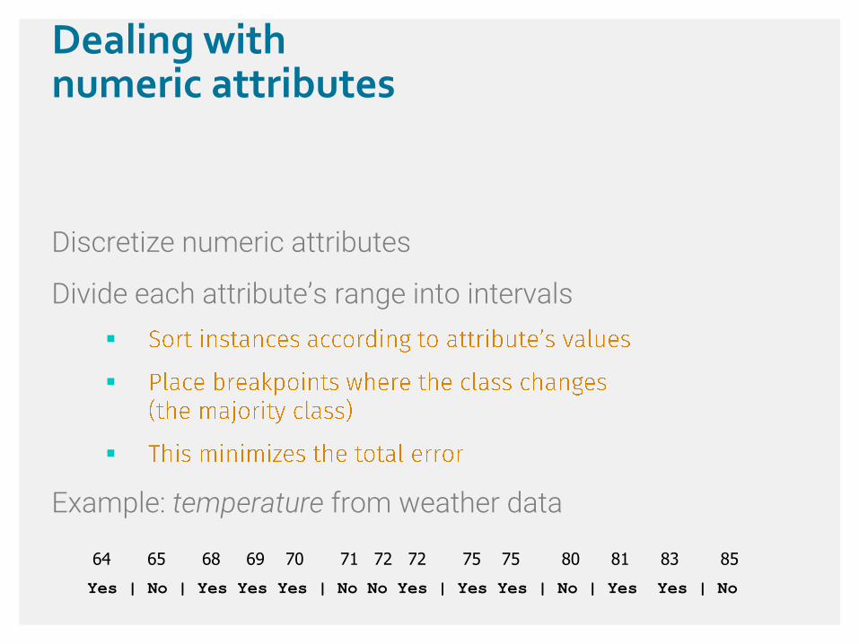
Dealing with numeric attributes

Discretize numeric attributes

Divide each attribute’s range into intervals

Example: temperature from weather data

64 65 68 69 70 71 72 72 75 75 80 81 83 85

Yes | No | Yes Yes Yes | No No Yes | Yes Yes | No | Yes Yes | No

Dealing with numeric attributes

Discretize numeric attributes

Divide each attribute’s range into intervals

Example: temperature from weather data

64 65 68 69 70 71 72 72 75 75 80 81 83 85

Yes | No | Yes Yes Yes | No No Yes | Yes Yes | No | Yes Yes | No

Outlook Temperature Humidity Windy Play

Sunny 85 85 False No

Sunny 80 90 True No

Overcast 83 86 False Yes

Rainy 75 80 False Yes

… … … … …

The problem of overfitting

This procedure is very sensitive to noise

Also: time stamp attribute will have zero errors

Simple solution: enforce minimum number of instances in majority class per interval

Discretization example

Example (with min = 3):

Final result for temperature attribute

64 65 68 69 70 71 72 72 75 75 80 81 83 85

Yes | No | Yes Yes Yes | No No Yes | Yes Yes | No | Yes Yes | No

64 65 68 69 70 71 72 72 75 75 80 81 83 85

Yes No Yes Yes Yes | No No Yes Yes Yes | No Yes Yes No

With overfitting avoidance

Resulting rule set:

Attribute Rules Errors Total errors

Outlook Sunny No 2/5 4/14

Overcast Yes 0/4

Rainy Yes 2/5

Temperature 77.5 Yes 3/10 5/14

> 77.5 No* 2/4

Humidity 82.5 Yes 1/7 3/14

> 82.5 and 95.5 No 2/6

> 95.5 Yes 0/1

Windy False Yes 2/8 5/14

True No* 3/6

Bayesian (Statistical) modeling

“Opposite” of 1R: use all the attributes

Two assumptions: Attributes are

Independence assumption is almost never correct!

But … this scheme works well in practice

Probabilities for weather data Outlook Temperature Humidity Windy Play

Yes No Yes No Yes No Yes No Yes No

Sunny 2 3 Hot 2 2 High 3 4 False 6 2 9 5

Overcast 4 0 Mild 4 2 Normal 6 1 True 3 3

Rainy 3 2 Cool 3 1

Sunny 2/9 3/5 Hot 2/9 2/5 High 3/9 4/5 False 6/9 2/5 9/14 5/14

Overcast 4/9 0/5 Mild 4/9 2/5 Normal 6/9 1/5 True 3/9 3/5

Rainy 3/9 2/5 Cool 3/9 1/5 Outlook Temp Humidity Windy Play

Sunny Hot High False No

Sunny Hot High True No

Overcast Hot High False Yes

Rainy Mild High False Yes

Rainy Cool Normal False Yes

Rainy Cool Normal True No

Overcast Cool Normal True Yes

Sunny Mild High False No

Sunny Cool Normal False Yes

Rainy Mild Normal False Yes

Sunny Mild Normal True Yes

Overcast Mild High True Yes

Overcast Hot Normal False Yes

Rainy Mild High True No

Probabilities for weather data

Outlook Temp. Humidity Windy Play

Sunny Cool High True ? A new day:

Likelihood of the two classes

For “yes” = 2/9 3/9 3/9 3/9 9/14 = 0.0053

For “no” = 3/5 1/5 4/5 3/5 5/14 = 0.0206

Conversion into a probability by normalization:

P(“yes”) = 0.0053 / (0.0053 + 0.0206) = 0.205

P(“no”) = 0.0206 / (0.0053 + 0.0206) = 0.795

Outlook Temperature Humidity Windy Play

Yes No Yes No Yes No Yes No Yes No

Sunny 2 3 Hot 2 2 High 3 4 False 6 2 9 5

Overcast 4 0 Mild 4 2 Normal 6 1 True 3 3

Rainy 3 2 Cool 3 1

Sunny 2/9 3/5 Hot 2/9 2/5 High 3/9 4/5 False 6/9 2/5 9/14 5/14

Overcast 4/9 0/5 Mild 4/9 2/5 Normal 6/9 1/5 True 3/9 3/5

Rainy 3/9 2/5 Cool 3/9 1/5

Bayes’s rule Probability of event H given evidence E :

A priori probability of H :

A posteriori probability of H :

]Pr[

]Pr[]|Pr[]|Pr[

E

HHEEH

]|Pr[ EH

]Pr[H

Thomas Bayes

Born: 1702 in London, England

Died: 1761 in Tunbridge Wells, Kent, England

from Bayes “Essay towards solving a problem in the

doctrine of chances” (1763)

Naïve Bayes for classification

Classification learning: what’s the probability of the class given an instance?

Naïve assumption: evidence splits into parts (i.e. attributes) that are independent

]Pr[

]Pr[]|Pr[]|Pr[]|Pr[]|Pr[ 21

E

HHEHEHEEH n

Weather data example

Outlook Temp. Humidity Windy Play

Sunny Cool High True ? Evidence E

Probability of

class “yes”

]|Pr[]|Pr[ yesSunnyOutlookEyes

]|Pr[ yesCooleTemperatur

]|Pr[ yesHighHumidity

]|Pr[ yesTrueWindy

]Pr[

]Pr[

E

yes

]Pr[

149

93

93

93

92

E

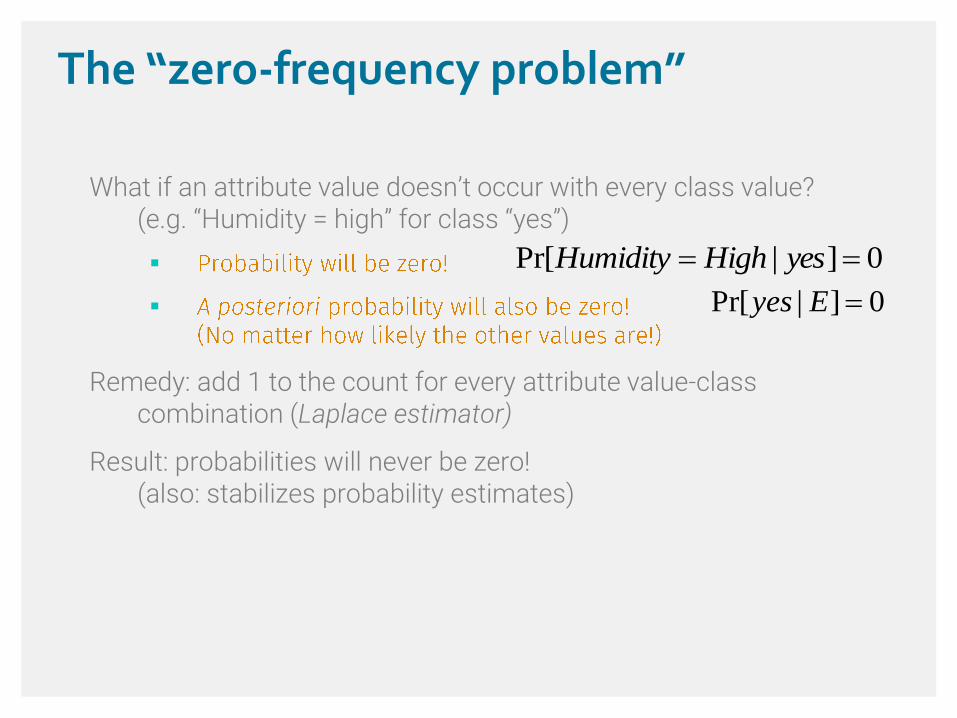
The “zero-frequency problem”

What if an attribute value doesn’t occur with every class value? (e.g. “Humidity = high” for class “yes”)

Remedy: add 1 to the count for every attribute value-class combination (Laplace estimator)

Result: probabilities will never be zero! (also: stabilizes probability estimates)

0]|Pr[ Eyes

0]|Pr[ yesHighHumidity

*Modified probability estimates

In some cases adding a constant different from 1 might be more appropriate

Example: attribute outlook for class yes

Weights don’t need to be equal (but they must sum to 1)

9

3/2

9

3/4

9

3/3

Sunny Overcast Rainy

9

2 1p

9

4 2p

9

3 3p

Missing values

Training: instance is not included in frequency count for attribute value-class combination

Classification: attribute will be omitted from calculation

Example:

Outlook Temp. Humidity Windy Play

? Cool High True ?

Likelihood of “yes” = 3/9 3/9 3/9 9/14 = 0.0238

Likelihood of “no” = 1/5 4/5 3/5 5/14 = 0.0343

P(“yes”) = 0.0238 / (0.0238 + 0.0343) = 41%

P(“no”) = 0.0343 / (0.0238 + 0.0343) = 59%

Numeric attributes Usual assumption: attributes have a normal or

Gaussian probability distribution (given the class)

The probability density function for the normal distribution is defined by two parameters:

n

i

ixn 1

1

n

i

ixn 1

2)(1

1

2

2

2

)(

2

1)(

x

exf Karl Gauss, 1777-1855 great German mathematician

Statistics for weather data

Example density value: 0340.0

2.62

1)|66(

2

2

2.62

)7366(

eyesetemperaturf

Outlook Temperature Humidity Windy Play

Yes No Yes No Yes No Yes No Yes No

Sunny 2 3 64, 68, 65, 71, 65, 70, 70, 85, False 6 2 9 5

Overcast 4 0 69, 70, 72, 80, 70, 75, 90, 91, True 3 3

Rainy 3 2 72, … 85, … 80, … 95, …

Sunny 2/9 3/5 =73 =75 =79 =86 False 6/9 2/5 9/14 5/14

Overcast 4/9 0/5 =6.2 =7.9 =10.2 =9.7 True 3/9 3/5

Rainy 3/9 2/5

Classifying a new day

A new day:

Missing values during training are not included in calculation of mean and standard deviation

Outlook Temp. Humidity Windy Play

Sunny 66 90 true ?

Likelihood of “yes” = 2/9 0.0340 0.0221 3/9 9/14 = 0.000036

Likelihood of “no” = 3/5 0.0291 0.0380 3/5 5/14 = 0.000136

P(“yes”) = 0.000036 / (0.000036 + 0. 000136) = 20.9%

P(“no”) = 0.000136 / (0.000036 + 0. 000136) = 79.1%

Naïve Bayes: discussion

Naïve Bayes works surprisingly well (even if independence assumption is clearly violated)

Why? Because classification doesn’t require accurate probability estimates as long as maximum probability is assigned to correct class

However: adding too many redundant attributes will cause problems (e.g. identical attributes)

Note also: many numeric attributes are not normally distributed ( kernel density estimators)

Naïve Bayes Extensions

Improvements:

Bayesian Networks

Summary

OneR – uses rules based on just one attribute

Naïve Bayes – use all attributes and Bayes rules to estimate probability of the class given an instance.