MAC2313 Calculus III - Chapter 13
1
Functions of Several Variables13
Copyright © Cengage Learning. All rights reserved.
Introduction to Functions of Several Variables
Copyright © Cengage Learning. All rights reserved.
13.1
3
Understand the notation for a function of several variables.
Sketch the graph of a function of two variables.
Sketch level curves for a function of two variables.
Sketch level surfaces for a function of three variables.
Use computer graphics to graph a function of two variables.
Objectives
4
Functions of Several Variables
The work done by a force (W = FD) and the volume of a right circular cylinder (V = ) are both functions of two variables. The volume of a rectangular solid (V = lwh) is a function of three variables.
Examples:
and
5
Example 1 – Domains of Functions of Several Variables
Find the domain of each function.
a. b.
Solution:
a. The function f is defined for all points (x, y) such that
x 0 and
6
Example 1 – Solution
So, the domain is the set of all points lying on or outside
the circle , except those points on the y-axis,
as shown in Figure 13.1.
cont’d
Figure 13.1
MAC2313 Calculus III - Chapter 13
2
7
b. The function g is defined for all points (x, y, z) such that
Consequently, the domain is the set of all points (x, y, z)
lying inside a sphere of radius 3 that is centered at the
origin.
Example 1 – Solutioncont’d
8
Examples:
9
Examples: Evaluate
10
Examples: Evaluate
11
Examples:
12
Examples: Describe domain
MAC2313 Calculus III - Chapter 13
3
13
Examples: Sketch
14
The Graph of a Function of Two Variables
The graph of a function f of two variables is the set of all points (x, y, z) for which z = f(x, y) and (x, y) is in the domain of f.
Figure 13.2
15
Example 2 – Describing the Graph of a Function of Two Variables
What is the range of Describe the
graph of f.
Solution:
The domain D: all points (x, y) such that
So, D is the set of all points lying on or inside the ellipse
given by
16
Example 2 – Solution
The range of f is all values z = f(x, y) such that
or
To graph: rewrite the function:
cont’d
17
You know that the graph of f is the upper half of an ellipsoid,
as shown in Figure 13.3.
Figure 13.3
Example 2 – Solutioncont’d
18
A second way to visualize a function of two variables is to use a scalar field in which the scalar z = f(x, y) is assigned to the point (x, y).
A scalar field can be characterized by level curves (or contour lines) along which the value of f(x, y) is constant.
For instance, the weather map
in Figure 13.5 shows level curves
of equal pressure called isobars.
http://math.bu.edu/people/paul/225/spring01/class14.html
Figure 13.5
Level Curves
MAC2313 Calculus III - Chapter 13
4
19
In weather maps for which the level
curves represent points of equal
temperature, the level curves are
called isotherms, as shown in
Figure 13.6.
Another common use of level curves
is in representing electric potential fields.
In this type of map, the level curves are called equipotential lines.
Figure 13.6
Level Curves
20
Contour maps are commonly used to show regions on Earth’s surface, with the level curves representing the height above sea level. This type of map is called a topographic map.
For example, the mountain shown on the left is represented by the topographic map on the right.
Figure 13.7 Figure 13.8
Level Curves
21
Example 3 – Sketching a Contour Map
The hemisphere given by is shown in Figure 13.9. Sketch a contour map of this surface using level curves corresponding to c = 0, 1, 2,…, 8.
Figure 13.9 22
Example 3 – Solution
For each value of c, the equation given by f(x, y) = c is a circle (or point) in the xy-plane.
For example, when c1= 0, the level curve is
which is a circle of radius 8.
23
Figure 13.10 shows the nine level curves for the hemisphere.
cont’d
Figure 13.10
Example 3 – Solution
24
Examples:
MAC2313 Calculus III - Chapter 13
5
25
Examples: Sketch Level Curves
26
The concept of a level curve can be extended by one dimension to define a level surface.
If f is a function of three variables
and c is a constant, the graph of the
equation f( x, y, z) = c is a
level surface of the function f,
as shown in Figure 13.14.
Figure 13.14
Level Surfaces
27
With computers, engineers and scientists have developed other ways to view functions of three variables.
For instance, Figure 13.15
shows a computer simulation
that uses color to represent
the temperature distribution
of fluid inside a pipe fitting.
Figure 13.15
Level Surfaces
28
Figure 13.17 shows a computer-generated graph of this surface using 26 traces taken parallel to the yz-plane.
To heighten the three-dimensional effect, the program uses a “hidden line” routine.
Figure 13.17
Computer Graphics
29
Computer Graphics
30
cont’dComputer Graphics
MAC2313 Calculus III - Chapter 13
6
31
Limits and Continuity
Copyright © Cengage Learning. All rights reserved.
13.2
13.2 32
Limit of a Function of Two Variables
For functions of a single variable, the limit exists if the limit from the left is equal to the limit from the right.
For functions of two variables, the limit exists if the limits from all possible paths are equal.
13.2
33
For some functions, it is easy to recognize that a limit does not exist.
Limit of a Function of Two Variables
13.2 34
Continuity of a Function of Two Variables
13.2
35
Indeterminant forms
13.2 36
Indeterminant forms
13.2
MAC2313 Calculus III - Chapter 13
7
37
Indeterminant forms
13.2 38
Indeterminant forms
13.2
39
Indeterminant forms
13.2 40
Continuity of a Function of Two Variables
The functions whose graphs are shown are continuous at every point in the plane.
13.2
41
Example 5 – Testing for Continuity
Discuss the continuity of each function.
13.2 42
Example 5(a) – Solution
f is continuous at each point in the xy-plane except at (0, 0).
13.2
MAC2313 Calculus III - Chapter 13
8
43
Example 5(b) – Solution
The function given by
g(x, y) = 2/(y – x2) is continuous except at the points at which the denominator is 0,
y – x2 = 0.
The function is continuous at all points except those lying on the parabola y = x2.
cont’d
13.2 44
Partial Derivatives
Copyright © Cengage Learning. All rights reserved.
13.3
Objective:
Find and use partial derivatives and higher-order partial derivatives of a function of two or three variables.
13.3
45
Partial Derivative Symbol ∂
∂ is a mathematical symbol, derived from Greek delta, used to denote a partial derivative.
∂ is different than the straight d of total derivative notation.
13.3 46
If z = f(x, y), then to find fx you consider y constant and differentiate with respect to x.
Similarly, to find fy, you consider x constant and differentiate with respect to y.
Partial Derivatives of a Function of Two Variables
13.3
47
Example 1 – Finding Partial Derivatives
Find the partial derivatives fx and fy for the function
f(x, y) = 3x – x2y2 + 2x3y.
Solution:
Considering y to be constant and differentiating with respect to x produces
f(x, y) = 3x – x2y2 + 2x3y Write original function.
fx(x, y) = 3 – 2xy2 + 6x2y. Partial derivative with respect to x
13.3 48
Example 1 – Solution
Considering x to be constant and differentiating with respect
to y produces
f(x, y) = 3x – x2y2 + 2x3y Write original function.
fy(x, y) = –2x2y + 2x3. Partial derivative with respect to y
cont’d
13.3
MAC2313 Calculus III - Chapter 13
9
49
Geometric interpretation: fx gives the slope in the x-direction
fy gives the slope in the y-direction
Partial Derivatives of a Function of Two Variables
13.3 50
Example 3 – Finding the Slopes of a Surface in the x- and y-Directions
Find the slopes in the x-direction and in the y-direction of the surface given by
Solution:
The partial derivatives of f with respect to x and y are
13.3
51
Example 3 – Solution
So, in the x-direction, the slope is
and in the y-direction the slope is
Figure 13.31(a) Figure 13.31(b)
cont’d
13.3 52
Partial Derivatives of a Function of Three or More Variables
13.3
53
a. To find the partial derivative of f(x, y, z) = xy + yz2 + xz with respect to z, consider x and y to be constant and obtain
b. To find the partial derivative of f(x, y, z) = z sin(xy2 + 2z) with respect to z, consider x and y to be constant and obtain
Example 6 – Finding Partial Derivatives
13.3 54
Example 6 – Finding Partial Derivatives
c. To find the partial derivative of f(x, y, z, w) = (x + y + z)/w with respect to w, consider x ,y, and z to be constant obtain
cont’d
13.3
MAC2313 Calculus III - Chapter 13
10
55
Higher-Order Partial Derivatives
The function z = f(x, y) has the following second partial derivatives.
1. Differentiate twice with respect to x:
2. Differentiate twice with respect to y:
3. Differentiate first with respect to x and then with respect
to y:
13.3 56
4. Differentiate first with respect to y and then with respect to x:
The third and fourth cases are called mixed partial derivatives.
Higher-Order Partial Derivatives
13.3
57
Example 7 – Finding Second Partial Derivatives
Find the second partial derivatives of
f(x, y) = 3xy2 – 2y + 5x2y2, and determine the value of
fxy(–1, 2).
Solution:
Begin by finding the first partial derivatives with respect to xand y.
fx(x, y) = 3y2 + 10xy2 and fy(x, y) = 6xy – 2 + 10x2y
Then, differentiate each of these with respect to x and y.
fxx(x, y) = 10y2 and fyy(x, y) = 6x + 10x2
13.3 58
Example 7 – Solution
fxy(x, y) = 6y + 20xy and fyx(x, y) = 6y + 20xy
At (–1, 2) the value of fxy is fxy(–1, 2) = 12 – 40 = –28.
cont’d
13.3
59
Examples
13.3 60
Examples
13.3
MAC2313 Calculus III - Chapter 13
11
61
Examples
13.3 62
Differentials
Copyright © Cengage Learning. All rights reserved.
13.4Objectives:Understand the concepts of increments and
differentials. Extend the concept of differentiability to a function
of two variables.Use a differential as an approximation.
13.4
63
Increments and Differentials
This definition can be extended to a function of three ormore variables.
For instance, if w = f(x, y, z, u), then dx = ∆x, dy = ∆y, dz = ∆z, du = ∆u, and the total differential of w is
13.4 64
Example 1 – Finding the Total Differential
Find the total differential for each function.
a. z = 2x sin y – 3x2y2 b. w = x2 + y2 + z2
Solution:
a. The total differential dz for z = 2x sin y – 3x2y2 is
= (2 sin y – 6xy2)dx + (2x cos y – 6x2y)dy.
13.4
65
Example 1– Solution
b. The total differential dw for w = x2 + y2 + z2 is
= 2x dx + 2y dy + 2z dz.
cont’d
13.4 66
Additional Examples
13.4
MAC2313 Calculus III - Chapter 13
12
67
Additional Examples
13.4 68
Propagated and Relative Error
13.4
69
Volume of a Cylinder
13.4 70
Example 3 – Using a Differential as an Approximation
Use the differential dz to approximate the change in
z = as (x, y) moves from the point (1, 1) to the point (1.01, 0.97). Compare this approximation with the exact change in z.
13.4
71
Example 3 – SolutionLetting (x, y) = (1, 1) and (x + ∆x, y + ∆y) = (1.01, 0.97) produces dx = ∆x = 0.01 and dy = ∆y = –0.03.
So, the change in z can be approximated by
∆z ≈ dz
When x = 1 and y = 1, you have
∆z ≈
13.4 72
In Figure 13.36, you can see that the exact change corresponds to the difference in the heights of two points on the surface of a hemisphere.
This difference is given by
∆z = f(1.01, 0.97) – f(1, 1)
≈ 0.0137
Figure 13.36
Example 3 – Solution cont’d
13.4
MAC2313 Calculus III - Chapter 13
13
73
Chain Rules for Functions of Several Variables
Copyright © Cengage Learning. All rights reserved.
13.5
Objectives
Use the Chain Rules for functions of several variables.
Find partial derivatives implicitly.
13.5 74
Chain Rules for Functions of Several Variables
13.5
75
Example 1 – Using the Chain Rule with One Independent Variable
Let w = x2y – y2, where x = sin t and y = et. Find dw/dt
when t = 0.
Solution:
By the Chain Rule for one independent variable, you have
13.5 76
Example 1 – Solution
When t = 0, it follows that
cont’d
13.5
77
The Chain Rule in Theorem 13.6 can be extended to any
number of variables. For example, if each xi is a
differentiable function of a single variable t, then for
w = f(x1, x2, . . . , xn)
you have
Chain Rules for Functions of Several Variables
13.5 78
Chain Rules for Functions of Several Variables
13.5
MAC2313 Calculus III - Chapter 13
14
79
Use the Chain Rule to find w/s and w/t for
w = 2xy
where x = s2 + t2 and y = s/t.
Solution:
Using Theorem 13.7, you can hold t constant and
differentiate with respect to s to obtain
Example 4 – The Chain Rule with Two Independent Variables
13.5 80
Similarly, holding s constant gives
Example 4 – Solutioncont’d
13.5
81
Example 4 – Solutioncont’d
13.5 82
Examples using the chain rule with partial derivatives
13.5
83
Examples using the chain rule with partial derivatives
13.5 84
Examples using the chain rule with partial derivatives
13.5
MAC2313 Calculus III - Chapter 13
15
85
Suppose that x and y are related by the equation F(x, y) = 0,
where it is assumed that y = f(x) is a differentiable function
of x. To find dy/dx use chain rule.
If you consider the function given by
w = F(x, y) = F(x, f(x))
you can apply Theorem 13.6 to obtain
Implicit Partial Differentiation
13.5 86
Because w = F(x, y) = 0 so dw/dx = 0 and
Now, if Fy(x, y) ≠ 0, use dx/dx = 1 to conclude
Implicit Partial Differentiation
13.5
87
Implicit Partial Differentiation
13.5 88
Find dy/dx, given y3 + y2 – 5y – x2 + 4 = 0.
Solution:
Begin by defining a function F as
F(x, y) = y3 + y2 – 5y – x2 + 4.
Then, using Theorem 13.8, you have
Fx(x, y) = –2x and Fy(x, y) = 3y2 + 2y – 5
and it follows that
Example 6 – Finding a Derivative Implicitly
13.5
8913.5 90
Directional Derivatives and Gradients
Copyright © Cengage Learning. All rights reserved.
13.6
13.6
MAC2313 Calculus III - Chapter 13
16
91
Find and use directional derivatives of a function of two variables.
Find the gradient of a function of two variables.
Use the gradient of a function of two variables in applications.
Find directional derivatives and gradients of functions of three variables.
Objectives
13.6 92
Directional Derivative
You are standing on the hillside pictured and want to determine the hill’s incline toward the z-axis.
13.6
93
If the hill were represented by z = f(x, y),
the slope in the y-direction would be fy(x, y)
the slope in the x-direction would be fx(x, y).
These two partial derivatives can be used to find the
slope in any direction.
Directional Derivative
13.6 94
To determine the slope at a point on a surface find a directional derivative.
Let z = f(x, y) be a surface and P(x0, y0) be a point in the domain.
The “direction” of the directional
derivative is given by a unit vector
u = cos i + sin j
where is the angle the vector
makes with the positive x-axis.
Directional Derivative
13.6
9513.6 96
Directional Derivative
13.6
MAC2313 Calculus III - Chapter 13
17
97
There are infinitely many directional derivatives of a surface at a given point—one for each direction specified by u, as shown.
Directional Derivative
13.6 98
Example 1 – Finding a Directional Derivative
Find the directional derivative of
at (1, 2) in the direction of
13.6
99
Example 1 – Solution
Because fx and fy are continuous, f is differentiable, and you can apply Theorem 13.9.
Evaluating at = /3, x = 1, and y = 2 produces
Figure 13.4613.6 100
Examples: Directional Derivatives
13.6
101
Examples: Directional Derivatives
13.6 102
Examples: Directional Derivatives
13.6
MAC2313 Calculus III - Chapter 13
18
103
Examples: Directional Derivatives
13.6 104
The Gradient of a Function
For a function f(x,y,z) of 3 variables
13.6
105
The Gradient of a Function of Two Variables
13.6 106
Example 3 – Finding the Gradient of a Function
Find the gradient of f(x, y) = y ln x + xy2 at the point (1, 2).
Solution:
Using
and
you have
At the point (1, 2), the gradient is
13.6
107
Example
13.6 108
Applications of the Gradient
13.6
MAC2313 Calculus III - Chapter 13
19
109
Example 5 – Finding the Direction of Maximum Increase
The temperature in degrees Celsius on the surface of a metal plate is
T(x, y) = 20 – 4x2 – y2
where x and y are measured in centimeters. In what direction from (2, –3) does the temperature increase most rapidly? What is this rate of increase?
Solution:
The gradient is
T(x, y) = Tx(x, y)i + Ty(x, y)j
= –8xi – 2yj.
13.6 110
Example 5 – Solution
It follows that the direction of maximum
increase is given by
T(2, –3) = –16i + 6j
as shown in Figure 13.51,
and the rate of increase is
||T(2, –3)||
Figure 13.51
cont’d
13.6
111
Example 8 – Finding the Gradient for a Function of Three Variables
Find f(x, y, z) for the function given by
f(x, y, z) = x2 + y2 – 4z
and find the direction of maximum increase of f at the point
(2, –1, 1).
Solution:
The gradient vector is given by
f(x, y, z) = fx(x, y, z)i + fy(x, y, z)j + fz(x, y, z)k
= 2xi + 2yj – 4k
13.6 112
Example 8 – Solution
So, it follows that the direction of maximum increase at
(2, –1, 1) is
f(2, –1, 1) = 4i – 2j – 4k.
cont’d
13.6
113
Example
13.6 114
Links
Topographic Map - Hikers
http://www.mathgraphs.com/calc9e/mg13f01002.pdf
Isobars
http://www.mathgraphs.com/calc9e/mg13f01003.pdf
13.6
MAC2313 Calculus III - Chapter 13
20
115
Tangent Planes and Normal Lines
Copyright © Cengage Learning. All rights reserved.
13.7
13.7 116
Tangent Plane and Normal Line to a Surface
You can represent the surfaces in space primarily by equations of the form
z = f(x, y). Equation of a surface S
In the development to follow, however, it is convenient to use the more general representation
F(x, y, z) = 0. Alternative equation of surface S
Convert z = f(x, y), to the general form by defining F as
F(x, y, z) = f(x, y) – z.13.7
117
Example 1 – Writing an Equation of a Surface
For the function given by
F(x, y, z) = x2 + y2 + z2 – 4
describe the level surface given by F(x, y, z) = 0.
Solution:
The level surface given by F(x, y, z) = 0 can be written as
x2 + y2 + z2 = 4
which is a sphere of radius 2 whose center is at the origin.
13.7 118
Normal lines are important in analyzing surfaces and solids.
For example, consider the collision of two billiard balls.
When a stationary ball is struck at a point P on its surface, it moves along the line of impact determined by P and the center of the ball.
The impact can occur in two ways. If the cue ball is moving along the line of impact, it stops dead and imparts all of its momentum to the stationary ball, as shown.
Tangent Plane and Normal Line to a Surface
13.7
119
If the cue ball is not moving along the line of impact, it is deflected to one side or the other and retains part of its momentum.
That part of the momentum that is transferred to the stationary ball occurs along the line of impact, regardless of the direction of the cue ball, as shown.
This line of impact is
called the normal line
to the surface of
the ball at the point P.
Tangent Plane and Normal Line to a Surfacecont’d
13.7 120
Lines & Planes in Space
13.7
MAC2313 Calculus III - Chapter 13
21
121
Tangent Plane and Normal Line to a Surface
13.7 122
Tangent Plane and Normal Line to a Surface
13.7
123
Example 2 – Finding an Equation of a Tangent Plane
Find an equation of the tangent plane to the hyperboloid given by
z2 – 2x2 – 2y2 = 12
at the point (1, –1, 4).
Solution:
Begin by writing the equation of the surface as
z2 – 2x2 – 2y2 – 12 = 0.
Then, considering
F(x, y, z) = z2 – 2x2 – 2y2 – 12
you have
Fx(x, y, z) = –4x, Fy(x, y, z) = –4y and Fz(x, y, z) = 2z.13.7 124
Example 2 – SolutionAt the point (1, –1, 4) the partial derivatives are
Fx(1, –1, 4) = –4, Fy(1, –1, 4) = 4, and Fz(1, –1, 4) = 8.
So, an equation of the tangent plane at (1, –1, 4) is
–4(x – 1) + 4(y + 1) + 8(z – 4) = 0
–4x + 4 + 4y + 4 + 8z – 32 = 0
–4x + 4y + 8z – 24 = 0
x – y – 2z + 6 = 0.
Figure 13.58 shows a portion of the
hyperboloid and tangent plane.Figure 13.58
cont’d
13.7
125
To find the equation of the tangent plane at a point on a surface given by z = f(x, y), you can define the function Fby
F(x, y, z) = f(x, y) – z.
Then S is given by the level surface F(x, y, z) = 0, and by Theorem 13.13 an equation of the tangent plane to S at the point (x0, y0, z0) is
Tangent Plane and Normal Line to a Surface
13.7 126
ExamplesFor the given surface, find the equation of the tangent plane and parametric equations for the normal line at the given point.
13.7
MAC2313 Calculus III - Chapter 13
22
127
ExamplesFor the given surface, find the equation of the tangent plane and parametric equations for the normal line at the given point.
13.7 128
ExamplesFor the given surface, find the equation of the tangent plane and parametric equations for the normal line at the given point.
13.7
129
Extrema of Functions of Two Variables
Copyright © Cengage Learning. All rights reserved.
13.8
Objectives
Find absolute and relative extrema of a function of two variables.
Use the Second Partials Test to find relative extrema of a function of two variables.
13.8 130
Absolute Extrema and Relative Extrema
13.8
131
Absolute Extrema and Relative Extrema
To locate relative extrema of f, you can investigate the points at which the gradient of f is 0 or does not exist.
13.8 132
Absolute Extrema and Relative Extrema
Figure 13.6613.8
MAC2313 Calculus III - Chapter 13
23
133
Example 1 – Finding a Relative Extremum
Determine the relative extrema of
f(x, y) = 2x2 + y2 + 8x – 6y + 20.
Solution:
Begin by finding the critical points of f.
Because
fx(x, y) = 4x + 8 Partial with respect to x
and
fy(x, y) = 2y – 6 Partial with respect to y
are defined for all x and y, the only critical points are those for which both first partial derivatives are 0. 13.8 134
Example 1 – Solution
To locate these points, set fx(x, y) and fy(x, y) equal to 0, and solve the equations
4x + 8 = 0 and 2y – 6 = 0
to obtain the critical point (–2, 3).
By completing the square, you can conclude that for all
(x, y) ≠ (–2, 3)
f(x, y) = 2(x + 2)2 + (y – 3)2 + 3 > 3.
So, a relative minimum of f occurs at (–2, 3).
cont’d
13.8
135
Example 1 – Solution
The value of the relative minimum is f(–2, 3) = 3, as shown in Figure 13.67.
Figure 13.67
cont’d
13.8 136
The Second Partials Test
The critical points of a function of two variables do not always yield relative maxima or minima.
Some critical points yield saddle points, which are neither relative maxima nor relative minima.
13.8
137
The Second Partials Test
13.8 138
Example 3 – Using the Second Partials Test
Find the relative extrema of
f(x, y) = –x3 + 4xy – 2y2 + 1.
Solution:
Begin by finding the critical points of f.
Because
fx(x, y) = –3x2 + 4y
and
fy(x, y) = 4x – 4y
exist for all x and y, the only critical points are those for which both first partial derivatives are 0.
13.8
MAC2313 Calculus III - Chapter 13
24
139
Example 3 – Solution
To locate these points, set fx(x, y) and fy(x, y) equal to 0 to obtain
–3x2 + 4y = 0 and 4x – 4y = 0.
From the second equation you know that x = y, and, by substitution into the first equation, you obtain two solutions:
y = x = 0 and
cont’d
13.8 140
Example 3 – Solution
Because
it follows that, for the critical point (0, 0),
and, by the Second Partials Test, you can conclude that
(0, 0, 1) is a saddle point of f.
cont’d
13.8
141
Furthermore, for the critical point
and because you can conclude
that f has a relative maximum at as
shown in Figure 13.70.
Example 3 – Solutioncont’d
Figure 13.7013.8 142
Examples: Find relative extrema
13.8
143
Examples: Find relative extrema
13.8 144
Examples: Find relative extrema
13.8
MAC2313 Calculus III - Chapter 13
25
145
Applications of Extrema of Functions of Two Variables
Copyright © Cengage Learning. All rights reserved.
13.9
Objective:
Solve optimization problems involving functions of several variables.
13.9 146
Example 1 – Finding Maximum Volume
A rectangular box is resting on the xy-plane with one vertex at the origin. The opposite vertex lies in the plane
6x + 4y + 3z = 24
as shown. Find the maximum volume of such a box.
13.9
147
Example 1 – Solution
Let x, y, and z represent the length, width, and height of the box.
Because one vertex of the box lies in the plane 6x + 4y + 3z = 24, you know that , and you can write the volume xyz of the box as a function of two variables.
13.9 148
Example 1 – Solution
By setting the first partial derivatives equal to 0
you obtain the critical points (0, 0) and .
At (0, 0) the volume is 0, so that point does not yield a maximum volume.
cont’d
13.9
149
Example 1 – Solution
At the point , you can apply the Second Partials Test.
Because
and
cont’d
13.9 150
Example 1 – Solution
you can conclude from the Second Partials Test that the maximum volume is
Note that the volume is 0 at the boundary points of the triangular domain of V.
cont’d
13.9
MAC2313 Calculus III - Chapter 13
26
151
Applications: Optimization
13.9 152
Applications: Optimization
13.9
153
Applications: Optimization
13.9 154
Lagrange Multipliers
Copyright © Cengage Learning. All rights reserved.
13.10
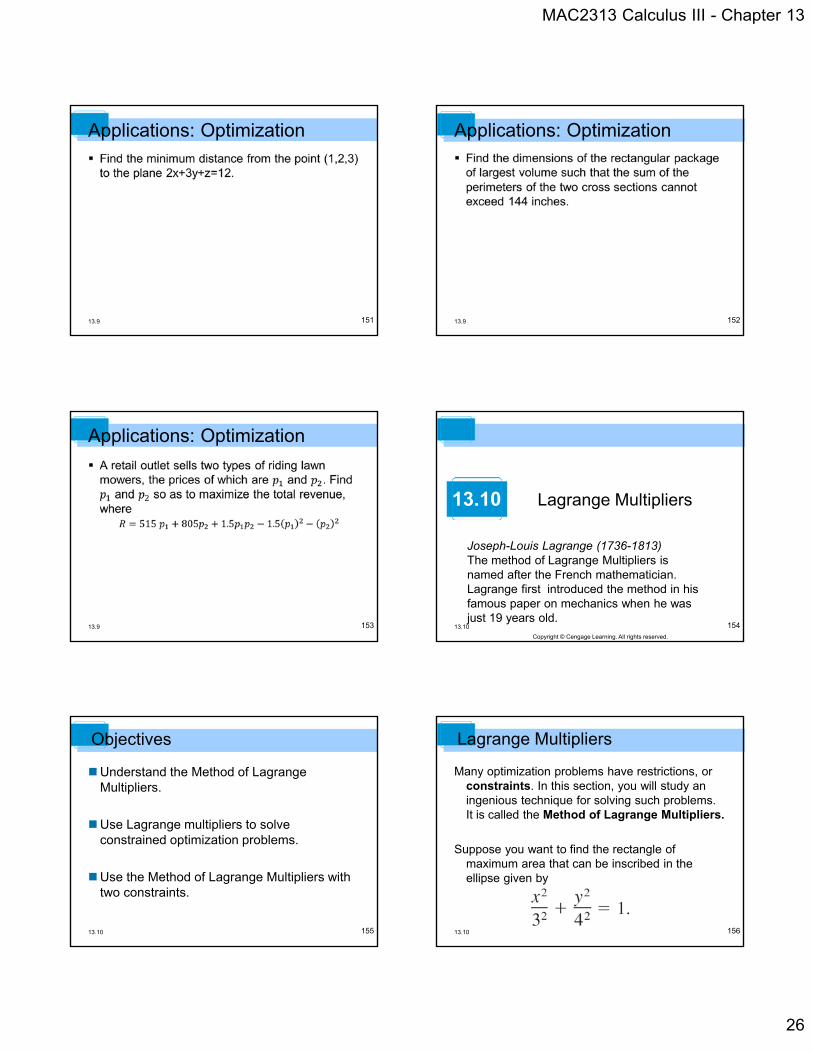
Joseph-Louis Lagrange (1736-1813) The method of Lagrange Multipliers is named after the French mathematician. Lagrange first introduced the method in his famous paper on mechanics when he was just 19 years old.
13.10
155
Understand the Method of Lagrange Multipliers.
Use Lagrange multipliers to solve constrained optimization problems.
Use the Method of Lagrange Multipliers with two constraints.
Objectives
13.10 156
Lagrange Multipliers
Many optimization problems have restrictions, or constraints. In this section, you will study an ingenious technique for solving such problems. It is called the Method of Lagrange Multipliers.
Suppose you want to find the rectangle of maximum area that can be inscribed in the ellipse given by
13.10
MAC2313 Calculus III - Chapter 13
27
157
Objective function
Maximize f(x, y) = 4xy.
Constraint
Lagrange Multipliers
13.10 158
Find the level curve of f(x,y)=4xy
that just satisfies the constraint (tangent).
At this point the gradients of f(x,y) and g(x,y) are parallel.
Lagrange Multipliers
13.10
159
If f(x, y) = g(x, y) then scalar is called
Lagrange multiplier.
Lagrange Multipliers
13.10 160
Lagrange Multipliers
13.10
161
Example 1 – Using a Lagrange Multiplier with One Constraint
Find the maximum value of f(x, y) = 4xy where x > 0 and
y > 0, subject to the constraint (x2/32) + (y2/42) = 1.
Solution:
To begin, let
By equating f(x, y) = 4yi + 4xj and
g(x, y) = (2x/9)i + (y/8)j, you can obtain the following system of equations.
13.10 162
Example 1 – Solution
From the first equation, you obtain = 18y/x, and substitution into the second equation produces
Substituting this value for x2 into the third equation produces
cont’d
13.10