LASSO-Driven Inference in Time and Space Victor Chernozhukov Wolfgang K. Härdle Chen Huang Weining Wang The Institute for Fiscal Studies Department of Economics, UCL cemmap working paper CWP20/19
Transcript
LASSO-Driven Inference in Time and Space
Victor ChernozhukovWolfgang K. HärdleChen HuangWeining Wang
The Institute for Fiscal Studies Department of Economics, UCL
cemmap working paper CWP20/19
LASSO-Driven Inference in Time and Space ∗
Victor Chernozhukov†, Wolfgang K. Härdle‡, Chen Huang§, Weining Wang¶
April 25, 2019
Abstract
We consider the estimation and inference in a system of high-dimensional regression equationsallowing for temporal and cross-sectional dependency in covariates and error processes, coveringrather general forms of weak dependence. A sequence of regressions with many regressors usingLASSO (Least Absolute Shrinkage and Selection Operator) is applied for variable selection purpose,and an overall penalty level is carefully chosen by a block multiplier bootstrap procedure to accountfor multiplicity of the equations and dependencies in the data. Correspondingly, oracle propertieswith a jointly selected tuning parameter are derived. We further provide high-quality de-biasedsimultaneous inference on the many target parameters of the system. We provide bootstrap con-sistency results of the test procedure, which are based on a general Bahadur representation for theZ-estimators with dependent data. Simulations demonstrate good performance of the proposedinference procedure. Finally, we apply the method to quantify spillover effects of textual sentimentindices in a financial market and to test the connectedness among sectors.
JEL classification: C12, C22, C51, C53Keywords: LASSO, time series, simultaneous inference, system of equations, Z-estimation, Bahadurrepresentation, martingale decomposition
1 Introduction
Many applications in statistics, economics, finance, biology and psychology are concerned witha system of ultra high-dimensional objects that communicate within complex dependency chan-nels. Given a complex system involving many factors, one builds a network model by takinga large set of regressions, i.e. regressing every factor in the system on a large subset of otherfactors. Examples include analysis of financial systemic risk by quantile predictive graphical∗We thank Weibiao Wu, Oliver Linton, Bryan Graham, Manfred Deistler, Hashem Pesaran, Michael Wolf,
Valentina Corradi, Zudi Lu, Liangjun Su, Peter Phillips, Frank Windmeijer, Wenyang Zhang and Likai Chenfor helpful comments and suggestions. We remain responsible for any errors or omissions. Financial supportfrom the Deutsche Forschungsgemeinschaft via IRTG 1792 “High Dimensional Non Stationary Time Series”,Humboldt-Universität zu Berlin, is gratefully acknowledged.†Department of Economics and Center for Statistics and Data Science, Massachusetts Institute of Technology.‡Ladislaus von Bortkiewicz Chair of Statistics, Humboldt-Universität zu Berlin. Sim Kee Boon Institute for
Financial Economics, Singapore Management University. The Wang Yanan Institute for Studies in Economics,Xiamen University. Department of Mathematics and Physics Charles University Prague.
§Faculty of Mathematics and Statistics, University of St. Gallen. Corresponding author: [email protected]¶Department of Economics, City, University of London. Ladislaus von Bortkiewicz Chair of Statistics,
Humboldt-Universität zu Berlin.
1
models with LASSO (Hautsch et al., 2015; Härdle et al., 2016; Belloni et al., 2016), limit or-der book network modeling via the penalized vector autoregressive approach (Härdle et al.,2018), analysis of psychology data with temporal and cross- sectional dependencies (Epskampet al. (2016)). Another example is quantifying the spillover effects or externalities for a socialnetwork, especially when the social interactions (or the interconnectedness) is not obvious (Man-resa, 2013). Besides, there are numerous applications concerning association network analysisin other fields of applied statistics, see Chapter 7 in Kolaczyk and Csárdi (2014) and Epskampet al. (2018). In general, a step-by-step LASSO procedure is very helpful for the correlationnetwork formation. In pursuing a highly structural approach, one certainly favors a simple setof regressions that allows multiple insights on the statistical structure of the data. Therefore,a sequence of regressions with LASSO is a natural path to take. Especially in cases of reducedforms of simultaneous equation models and structural vector autoregressive (VAR) models, onecan attain valuable pre-information on the core structure by running a set of simple regressionswith LASSO shrinkage.
A first important question arising in this framework is how to decide on a unified level ofpenalty. In this article we advocate an approach to selecting the overall level of the tuning pa-rameter in a system of equations after performing a set of single step regressions with shrinkage.A feasible (block) bootstrap procedure is developed and the consistency of parameter estimationis studied. In addition, we provide a uniform near-oracle bound for the joint estimators. Theproposed technique is applicable to ultra-high dimensional systems of regression equations withhigh-dimensional regressors.
A second crucial issue is to establish simultaneous inference on parameters, which is an im-portant question regarding network topology inference.For example, in a large-scale linear factorpricing model, it is of great interest to check the significance of the intercepts of cross sectionalregressions (connected with zero pricing errors), e.g. Pesaran and Yamagata (2017). Our ap-proach is an alternative testing solution compared to the Wald test statistics proposed therein.To achieve the goal of simultaneous inference, we develop a uniform robust post-selection orpost-regularization inference procedure for time series data. This method is generated froma uniform Bahadur representation of de-biased instrumental variable estimators. In particu-lar, we need to establish maximal inequalities for empirical processes for a general Huber’sZ-estimation. Note that the commonly used technique for independent data, such as the sym-metrization technique, is not directly applicable in the dependent data case, see Chapter 11.6of Kosorok (2008) for a related overview.
Our contribution lies in three aspects. First, we select the penalty level by controllingthe aggregated errors in a system of high-dimensional sparse regressions, and we establish thebounds on the estimated coefficients. Furthermore, we show the implication of the restrictedeigenvalue (RE) condition at a population level. Secondly, an easily implemented algorithmfor effective estimation and inference is proposed. In fact, the offered estimation scheme al-lows us to make local and global inference on any set of parameters of interest. Thirdly, werun numerical experiments to illustrate good performance of our joint penalty relative to thesingle equation estimation, and we show the finite sample improvement of our multiplier blockbootstrap procedure on the parameter inference. Finally, an application of textual sentiment
2
spillover effects on the stock returns in a financial market is presented.In the literature, the fundamental results on achieving near oracle rate for penalized `1-
norm estimators are developed by Bickel et al. (2009). There are many related articles onderiving near-oracle bounds using the `1-norm penalization function for the i.i.d. case, such asBelloni et al. (2011); Belloni and Chernozhukov (2013). There are also many extensions to theLASSO estimation with dependent data. For example, Kock and Callot (2015) consider thehigh-dimensional near-oracle inequalities in large vector autoregressive models. However, themajority of the literature imposes a sub-Gaussian assumption on the error distribution; thisis rather restrictive and excludes heavy tail distributions. For dependent data, Wu and Wu(2016) discuss the possibility of relaxing the sub-Gaussian assumption by generalizing Nagaev-type inequalities allowing for only moment assumptions. For the case of LASSO the analysisassumes the fixed design, which rules out the most important applications mentioned earlier inthe introduction.
Theoretically, the LASSO tuning parameter selection requires characterizing the asymptoticdistribution of the maximum of a high dimensional random vector. Chernozhukov et al. (2013a)develop a Gaussian approximation for the maximum of a sum of high-dimensional randomvectors, which is in fact the basic tool for modern high-dimensional estimation. Here it isapplied to the LASSO inference. Moreover, Chernozhukov et al. (2013b) deliver results for thecase of β-mixing processes. Although it is quite common to assume a mixing condition whichis at base a concept yielding asymptotic independence, it is not in general easy to verify thecondition for a particular process, and some simple linear processes can be excluded from thestrong mixing class, Andrews (1984). With an easily accessible dependency concept, Zhang andWu (2017a) derive Gaussian approximation results for a wide class of stationary processes. Notethat the dependence measure is linked to martingale decompositions and is therefore readilyconnected with a pool of results on tail probabilities, moment inequalities and central limittheorems of martingale theory. Our results are built on the above-mentioned theoretical worksand we extend them substantially to fit into the estimation in a system of regression equations.In particular, our LASSO estimation is with random design for dependent data; therefore, weneed to deal with the population implications of the Restricted Eigenvalue (RE) condition.Moreover, we show the interaction between the tail assumption and the dimensionality of thecovariates in our theoretical results.
In the meantime, the issue of simultaneous inference is challenging and has motivated aseries of research articles. For the case of i.i.d. data, Belloni et al. (2011, 2014), Zhang andZhang (2014), Javanmard and Montanari (2014), van de Geer et al. (2014), Neykov et al.(2015), Chernozhukov et al. (2016), Zhu and Bradic (2018), among others, develop confidenceintervals of low-dimensional variables in high-dimensional models with various forms of de-biased/orthogonalization methods. Still in the case of i.i.d. data, Belloni et al. (2015b) establisha uniform post-selection inference for the target parameters defined via de-biased Huber’s Z-estimators when the dimension of the parameters of interest is potentially larger than the samplesize, where they employ the multiplier bootstrap to the estimated residuals. Wild and residualbootstrap-assisted approaches are also studied in Dezeure et al. (2017); Zhang and Cheng (2017)for the case of mean regression. We pick up the line of the inference analysis of Belloni et al.
3
(2015b) and employ it in a temporal and cross-sectional dependence framework, thus making itapplicable to a rich class of high-dimensional time series. The core proof strategy is different,as it is well known that the technique for handling the suprema of empirical processes indexedby functional classes with dependent data is not the same as in i.i.d. cases. For instance, thekey Bahadur representation in Belloni et al. (2015b) applies maximal inequalities derived inChernozhukov et al. (2014) for i.i.d. random variables, while we derive the key concentrationinequalities based on a martingale approximation method.
Our proposed estimation framework is complement to the literature on model selection forGaussian Graphical model (GGM), see e.g. Yuan and Lin (2007), which has a wide spectrumof applications in statistics. A GGM can be connected with LASSO regression for estimatingsparse correlation networks, and therefore is equivalent to our context with a partial correla-tion network, Meinshausen et al. (2006). In particular, we may find an equation-by-equationrelationship to the GGM, and we acknowledge that a similar framework with spatial temporaldependence can be developed. In addition, there is a big literature on social network analysis,which embeds the network information into a dynamic model in advance, see for example Zhuet al. (2017, 2019); Chen et al. (2019); Huang et al. (2016). Relatively, our approach is lessstructural as we treat the network structure to be unknown and uncover it using LASSO.
The following notations are adopted throughout this paper. For a vector v = (v1, . . . , vp)>,let |v|∞
def= max16j6p |vj | and |v|sdef= (
∑pj=1 |vj |s)1/s, s > 1. For a random variable X, let
‖X‖qdef= (E |X|q)1/q, q > 0. For any function on a measurable space g : W → IR, En(g) def=
n−1∑nt=1g(ωt) and Gn(g) def= n−1/2∑n
t=1[g(ωt) − Eg(ωt)]. Given two sequences of positivenumbers xn and yn, write xn . yn if there exists constant C > 0 such that xn/yn 6 C. For anyfinitely discrete measure Q on a measurable space, let Lq(Q) denote the space of all measurablefunctions f : Z → IR such that ‖f‖Q,q
def= (Q|f |q)1/q < ∞, where Qf def=∫fdQ. For a class of
measurable functions F , the ε-covering number with respect to the Lq(Q)-semimetric is denotedas N (ε,F , ‖ · ‖Q,q), and let ent(ε,F) = log supQN (ε‖F‖Q,q,F , ‖ · ‖Q,q) with F = supf∈F |f |(the envelope) denote the uniform entropy number. It should be noted that we suppress thenotation of the outer expectation E∗ to E and outer probability P∗ to P when measurabilityissues are encountered. Details may be found in the Chapter 1 of Van Der Vaart and Wellner(1996).
The rest of the article is organized as follows. Section 2 shows the system model with afew examples. Section 3 introduces the sparsity method for effective prediction and providesan algorithm for the joint penalty level of LASSO via bootstrap. In Section 4 we proposeapproaches to implementing individual and simultaneous inference on the coefficients. Maintheorems are listed in Section 5. In Section 6 and 7 we deliver the simulation studies andan empirical application on textual sentiment spillover effects. The technical proofs and otherdetails are given in the supplementary materials. The codes to implement the algorithms arepublicly accessible via the website www.quantlet.de.
In this section, we present a general framework which covers many applications in statistics.Consider the system of regression equations (SRE):
Yj,t = X>j,tβ0j + εj,t, E εj,tXj,t = 0, j = 1, ..., J, t = 1, . . . , n,
where Xj,t = (Xjk,t)Kjk=1. Without loss of generality, we assume the dimension of the covariates
is identical among all equations thereafter, namely Kj = dim(Xj,t) ≡ K, for j = 1, . . . , J . Weallow the dimensionK ofXj,t and the number of equations, J to be large, potentially larger thann, which creates an interplay with the tail assumptions on the error processes εj,t. Both spatialand temporal dependency are allowed and we will obtain results on prediction and inference.
The SRE framework is a system of regression equations, which includes the following im-portant special cases.
Example 1 (Many Regression Models). Suppose that we are interested in estimating thepredictive models for the response variables Um,t:
It can be seen that we only put contemporaneous exogeneity conditions for Xt. It is worthmentioning that this SRE case is closely related to the semiparametric estimation frameworkstudied in Section 2.4 in Belloni et al. (2015b). Here, the understanding of the predictiverelations between covariates is important for constructing joint confidence intervals for the entireparameter vector (γ0
mk)Kk=1Mm=1 in the main regression equations. Indeed, the constructionrelies on the semi-parametrically efficient point estimators obtained from the empirical analogof the following orthogonalized moment equation:
E[(U0mk,t −Xk,tγ
0mk)νk,t] = 0, k = 1, . . . ,K, m = 1, . . . ,M, (2.1)
where U0mk,t = Um,t − X>−k,tγ0
m(−k) is the response variable minus the part explained by thecovariates other than k. Note that the empirical analog would have all unknown nuisanceparameters replaced by the estimators.
Example 2 (Simultaneous Equation Systems (SES)). Suppose there are many regression
5
equations in the following form:
Um,t = U>−m,tδ0m +X>t γ
0m + εm,t, m = 1, . . . ,M.
Move all the endogenous variables to the left-hand side and rewrite the model in the vectorform
DUt = ΓXt + εt,
which is also called the structural form of the model. Suppose that D is invertible. Then thecorresponding reduced form is given by
Ut = BXt + νt, E νm,tXt = 0, m = 1, . . . ,M, (2.2)
with B = D−1Γ and νt = D−1εt. In this case the Yj,t’s and Xj,t’s in SRE have no overlappingvariables. A high-dimensional SES can be considered as a special case of SRE with
Example 3 (Large Vector Autoregression Models). In the case where the covariatesinvolve lagged variables of the response, SRE can be written as a large vector autoregressionmodel. For example, the VAR(p) model,
Ut =p∑`=1
B`Ut−` + εt, E εm,tUt−` = 0, m = 1, . . . ,M, (2.3)
where Ut = (U1,t, U2,t, . . . , UM,t)>, and εt is anM -dimensional white noise or innovation process;see e.g. Chapter 2.1 in Lütkepohl (2005). It is a special SRE case again with
Such dynamics are of interest in biology to understand dynamic gene expression networkassociation using micro array data, see for example Opgen-Rhein and Strimmer (2007); Ramirezet al. (2017); Dimitrakopoulou et al. (2011). It is understood that a crucial feature for many genenetworks is their inherent sparsity. The issue of the number of variables involved is potentiallylarger than the sample size can be addressed by LASSO. Our methodology can help to analyzea gene interaction correlation network in a high dimensional regression scheme. In particular,suppose that each vertex represents a gene j collected at time point t with Uj,t as its geneexpression and an edge connects two genes if they are correlated.
We refer to Section C.1 in the supplementary materials for more practical examples.
3 Effective Prediction Using Sparsity Method
In this section, we present our model setup and the LASSO estimation algorithm, including thejoint penalty selection procedure.
6
3.1 Sparsity in SRE
The general SRE structure makes it possible to predict Yj,t using Xj,t effectively. Note that thedimension of Xj,t is large, potentially larger than n. Without loss of generality we assume exactsparsity of β0
j throughout the paper:
sj = |β0j |0 6 s = O(n), j = 1, . . . J. (3.1)
Comment 3.1. It is now well understood that sparsity can be easily extended to approximatesparsity, in which the sorted absolute values of coefficients decrease fast to zero. To bemore specific, when β0
jk is not sparse, we shall define an intermediary optimal value for ourtrue coefficients, i.e. β∗jk. Let LCp
def= min|βj |06p
[EnX>j,t(βj − β0j )2]1/2, additionally with proper
conditions on the design matrix, the optimal sparsity level is given by s∗j = min06p6(K∧n)
LC2p +
( max16k6K
Ψ2jk)p/n, where Ψ2
jk is the long run variance of 1√n
∑nt=1 εj,tXjk,t. Then the oracle β∗jk
is defined to be arg min|βj |06s∗j
EnX>j,t(βj − β0j )2. Thus an additional term involving LCs∗j will
appear in the bound in case of the true signal β0jk is not sparse. With approximate sparsity
we mean that the true signal is not sparse but nevertheless can be approximated by an exactsparsity set-up well, namely |β0
jk| 6 Ak−γ (ranked in descending order), where γ > 0.5, and bytaking s∗j ∝ n1/(2γ) the goal would be achieved.
For this situation one employs an `1-penalized estimator of β0j of the form:
βj = arg minβ∈IRK
1n
n∑t=1
(Yj,t −X>j,tβ)2 + λ
n
K∑k=1|βjk|Ψjk, (3.2)
where λ is the joint "optimal" penalty level and Ψjk’s are penalty loadings, which are definedbelow in (3.3).
A first aim is to obtain performance bounds with respect to the prediction norm:
|βj − β0j |j,pr
def=[ 1n
n∑t=1
X>j,t(βj − β0
j )2]1/2
,
where the outside j indicates to use the covariates in the jth equation Xj,t in computing theprediction norm, and the Euclidean norm:
|βj − β0j |2
def= K∑k=1
(βjk − β0jk)21/2
.
To achieve good performance bounds, we first consider "ideal" choices of the penalty level andthe penalty loadings. Let
Sjk = 1√n
n∑t=1
εj,tXjk,t,
where for a moment we assume to be able to observe εj,t = Yj,t−X>j,tβ0j . In practice one obtains
7
an approximation by stepwise LASSO. Set
Ψjkdef=√
avar(Sjk), (3.3)
λ0(1− α) def= (1− α)− quantile of 2c√n max
16j6J,16k6K|Sjk/Ψjk|, (3.4)
where c > 1, e.g., c = 1.1, and 1 − α is a confidence level, e.g. α = 0.1, where the long runvariance is denoted by avar.
Theoretically, we can characterize the rate of λ0(1 − α) by the tail probability of Sjk, seeTheorem 5.1, also via Gaussian Approximation as in corollary 5.4. To calculate λ0(1−α) fromdata, we can also use a Gaussian approximation based on:
Q(1− α) def= (1− α)− quantile of 2c√n max
16j6J,16k6K|Zjk/Ψjk|,
where Zjk are multivariate Gaussian centered random variables with the same long run co-variance structure as Sjk. Alternatively, we can employ a multiplier bootstrap procedure toestimate IC empirically to achieve a better finite sample performance; see for example Cher-nozhukov et al. (2013a). In case of dependent observations over time, it is understood that datacannot be resampled directly as in the the i.i.d. case, as the dependency structure of the under-lying processes will be lost. A usual solution to this problem is to consider a block bootstrapprocedure, where the data are grouped into blocks, resampled and concatenated. In particular,we will adopt an estimate of IC by a multiplier block bootstrap procedure. The theoreticalproperties of LASSO and the tuning parameter choices are presented in Section 5.1-5.4.
3.2 Multiplier Bootstrap for the Joint Penalty Level
In this subsection, we introduce an algorithm to approximate the joint penalty level via a blockmultiplier bootstrap procedure, which is particularly nonoverlapping block bootstrap (NBB).Consider the system of equations with dependent data:
Yj,t = X>j,tβ0j + εj,t, E εj,tXj,t = 0, j = 1, ..., J, t = 1, . . . , n, (3.5)
S1 Run the initial `1-penalized regression equation by equation, i.e. for the jth equation,
βj = arg minβ∈IRK
1n
n∑t=1
(Yj,t −X>j,tβ)2 + λjn
Kj∑k=1|βjk|Ψjk, (3.6)
where λj are the penalty levels and Ψjk are the penalty loadings. For instance, wecan take the X-independence choice using Gaussian approximation (in the heteroscedas-ticity case): 2c′
√nΦ−11 − α′/(2K) for λj , where Φ(·) denotes the cdf of N(0, 1),
α′ = 0.1, c′ = 0.5, and choose√
lvar(Xjk,tεj,t) for the penalty loadings, where εj,t arepreliminary estimated errors and lvar(Xjk,tεj,t) is an estimate of the long-run variance
8
∑∞`=−∞ E(Xjk,tεj,tXjk,(t−`)εj,(t−`)), e.g. the Newey-West estimator is given by
pn∑`=−pn
k(`/pn) cov(Xjk,tεj,t, Xjk,(t−`)εj,(t−`)),
with k(z) = (1−|z|)1(|z| 6 1). We note that the X-independent penalty (using Gaussianapproximation) is more conservative, as the correlations among regressors can be adaptedin the X-dependent case (using a multiplier bootstrap) with a less aggressive penalty level.
S2 Obtain the residuals for each equation by εj,t = Yj,t − X>j,tβj , and compute Ψjk =√lvar(Xjk,tεj,t).
S3 Divide εj,t into ln blocks containing the same number of observations bn, n = bnln,where bn, ln ∈ Z. Then choose λ = 2c
√nq
[B](1−α), where q
[B](1−α) is the (1 − α) quantile of
max16j6J,16k6K
|Z [B]jk /Ψjk|, and Z
[B]jk are defined as
Z[B]jk = 1√
n
ln∑i=1
ej,i
ibn∑l=(i−1)bn+1
εj,lXjk,l, (3.7)
ej,i are i.i.d. N(0, 1) random variables independent of the data.
The bootstrap consistency regarding Z [B]jk is proved in Theorem 5.3.
Comment 3.2 (Block bootstrap procedures). (i) Concerning the determination of bn, weshall report the prediction norm with several block sizes bn and select the one with thebest prediction performance in the simulation study. In addition, if it is the case that ncannot be divided by bn with no remainder, one can simply take ln = bn/bnc and dropthe remaining observations.
(ii) Other forms of multiplier bootstrap with any random multipliers centered around 0 canalso be considered.
(iii) Alternative block bootstrap procedures can be adopted, such as the circular bootstrapand the stationary bootstrap among others; see for example Lahiri et al. (1999) for anoverview.
4 Valid Inference on the Coefficients
With a reasonable fitting of LASSO on hand, we can proceed to investigate the issue of simul-taneous inference. This section focuses on SRE of Example 2. We allow the covariates in eachequation to be different.
The basic idea to facilitate inference is to formulate the estimation in a semi-parametricframework. With partialing out the effect of the nonparametric coefficient(s), we can achievethe desired estimation accuracy of the parametric component of interest. This trick is referredto as "Neyman orthogonalization". Notably, the procedure is equivalent to the well known de-sparsification procedure in the mean square loss case, which is developed for the inference on the
9
estimated zero coefficients by LASSO. It thus serves the same purpose of generating a (robust)de-sparsified estimation for LASSO inference.
We list three algorithms to estimate β0jk. Algorithm 1 is easy to implement and algorithm 2
is tailored to the cases of heavy-tailed distribution of the error term, as Least Absolute Deviation(LAD) regression is well known to be robust against outliers. Algorithm 3 considers a doubleselection procedure aimed at remedying the bias due to omitted variables by one step selection,while also accounting for the cases of heteroscedastic errors.
Algorithm 1: LS-based algorithm
S1 Consider Yj,t = Xjk,tβ0jk +X>j(−k),tβ
0j(−k) + εj,t, run (post) LS LASSO procedure (for each
j), and keep the quantity X>j(−k),tβ[1]j(−k) for each k.
S2 Run LASSO (for each j, k) by regressing Xjk,t = X>j(−k),tγ0j(−k) + vjk,t, and keep the
residuals as vjk,t = Xjk,t −X>j(−k),tγj(−k).
S3 Run LS IV regression of Yj,t−X>j(−k),tβ[1]j(−k) on Xjk,t using vjk,t as an instrument variable,
attaining the final estimator β[2]jk .
Algorithm 2: LAD-based algorithm
S1 and S2 are the same as Algorithm 1.
S3′ Run LAD IV regression of Yj,t −X>j(−k),tβ[1]j(−k) on Xjk,t using vjk,t as an instrument vari-
able, attaining the final estimator β[2]jk . We refer to Belloni et al. (2015b); Chernozhukov
and Hansen (2008) for more details about how to achieve the estimator in this step.
The theoretical properties of the estimators β[1]j(−k) and γj(−k) in S1 and S2 are provided
in Corollary 5.1 or 5.4 (see Corollary A.1 or A.4 in the supplementary correspondingly if thejoint penalty over equations is employed), and Theorem A.4 for post LASSO, respectively. Theuniform Bahadur representation and the Central Limit Theorem of the estimator β[2]
jk in S3 orS3′ are established in Theorem 5.4 and 5.5.
Comment 4.1. Our algorithms follow patterns discussed in Belloni et al. (2015b,a) in the i.i.d.settings. The IV estimator obtained in S3 of Algorithm 1 reduced to the de-biased LASSOestimator (Zhang and Zhang, 2014; van de Geer et al., 2014) and is also first-order equivalentto the double LASSO method in Belloni et al. (2011, 2014). In particular, the estimator underLS IV regression (2-step least square regression) is given by
β[2]jk = (v>jkXjk)−1v>jk(Yj −X>j(−k)β
[1]j(−k))
= (v>jkXjk)−1v>jkYj −∑m6=k
v>jkXjm
v>jkXjkβ
[1]jm. (4.1)
The second line in (4.1) is exactly the same as the de-biased or de-sparsified LASSO estimatorgiven in Eq. (5) in Zhang and Zhang (2014) or Eq. (5) in van de Geer et al. (2014). As remarkedin Belloni et al. (2015b,a), one can alternatively implement an algorithm via double selectionas in Belloni et al. (2011, 2014). In particular, heteroscedastic LASSO is employed in S2′′ and
10
the IV regression is replaced by a either LASSO or LAD regression on the target variable andall covariates selected in the first two steps.
Algorithm 3: Double selection-based algorithm
S1′′ Run LS LASSO (for each j) of Yj,t on Xj,t:
β[1]j = arg min
β
1n
n∑t=1
(Yj,t −X>j,tβ)2 + λ
n|Ψjβ|1.
S2′′ Run Heteroscedastic LASSO (for each j, k) of Xjk,t on Xj(−k),t:
γj(−k) = arg minγ
1n
n∑t=1
(Xjk,t −X>j(−k),tγ)2 + λ′
n|Γjγ|1,
where penalty loadings Γj can be initialized as√
lvarXj`,t(Xjk,t − 1n
∑nt=1Xjk,t) and
then refined by√
lvar(Xj`,tvjk,t), for ` 6= k, and vjk,t = Xjk,t − X>j(−k),tγj(−k) can beobtained by using the initial ones.
S3′′ Run LS regression of Yj,t on Xjk,t and the covariates selected in S1′′ and S2′′:
S3′′′ Run LAD regression of Yj,t on Xjk,t and the covariates selected in S1′′ and S2′′:
β[2]j = arg min
β 1n
n∑t=1|Yj,t −X>j,tβ| : supp(β−k) ⊆ supp(β[1]
j(−k)) ∪ supp(γj(−k)).
As shown in Belloni et al. (2011) and Belloni et al. (2015a), the double selection approach in S3′′
or S3′′′ creates an orthogonality condition with respect to the space spanned by the covariatesselected by both steps, and thus generates an orthogonal relation to any space spanned by alinear projection of the covariates, e.g. vjk,t. Therefore, the inference on the parameters maystill be applied as in the framework of Algorithm 1 and 2. Therefore, one may still find thetheoretical properties of estimators in S1′′, S2′′, S3′′ (S3′′′) in Section 5 according to the linksmentioned above.
4.1 Confidence Interval for a Single Coefficient
We discuss an inference framework developed for a single coefficient obtained from the afore-mentioned algorithms.
Let ψjk(Zj,t, βjk, hjk) denote the score function, where Zj,t = (Yj,t, X>j,t)>, hjk(Xj(−k),t) =(X>j(−k),tβj(−k), X
>j(−k),tγj(−k))>. Consider the LAD-based case with ψjk(Zj,t, βjk, hjk) = 1/2−
Suppose we are interested in testing H0 : β0jk = 0. For this purpose we employ the uniform
Bahadur representation (Theorem 5.4) to construct the confidence interval via a multiplierbootstrap procedure. In particular, the distribution of the asymptotically pivotal statistics:
Tjk =√n(β[2]
jk − β0jk)
σjk, (4.2)
is approximated via its block multiplier bootstrap counterpart:
T ∗jk = 1√n
ln∑i=1
ej,i
ibn∑l=(i−1)bn+1
ζjk,l, (4.3)
where ζjk,t are pre-estimators of ζjk,t = −φ−1jk σ
−1jk ψ
0jk,t such that max
(j,k),(j′,k′)|∑lni=1 ηj′k′,iηjk,i −∑ln
i=1 ηj′k′,iηjk,i| = OP(log(JK)−2), with ηjk,idef= 1√
n
∑ibnl=(i−1)bn+1 ζjk,l and
ηjk,idef= 1√
n
∑ibnl=(i−1)bn+1 ζjk,l, ej,i are independently drawn from N(0, 1), ln and bn are the
numbers of blocks and block size, respectively.Let σjk be any consistent estimator of σjk. Then the confidence interval is given by
CI∗jk(α) : [β[2]jk − σjkn
−1/2q∗jk(1− α), β[2]jk + σjkn
−1/2q∗jk(1− α)], (4.4)
where q∗jk(1− α) is the (1− α) quantile of the bootstrapped distribution of |T ∗jk|.
Comment 4.2 (Asymptotic Normality of β[2]jk ). As shown in Corollary 5.5 we have the limit
distribution of β[2]jk :
σ−1jk n
1/2(β[2]jk − β
0jk)
L→ N(0, 1), (4.5)
where σjk = (φ−2jk ωjk)1/2. Therefore, the two-sided 100(1−α) confidence interval by asymptotic
normality for β0jk is given by
CIjk(α) : [β[2]jk − σjkn
−1/2Φ−1(1− α/2), β[2]jk + σjkn
−1/2Φ−1(1− α/2)]. (4.6)
Comment 4.3 (Residual Multiplier Bootstrap). Alternative bootstrap procedures may be con-sidered as well, e.g. the residual multiplier bootstrap procedure:
εj,t = Yj,t −X>j,tβ[1]j ,
then divide εj,t into ln blocks of size bn, where bnln = n, and for each block i = 1, . . . , ln,
ε∗j,t = (εj,t −1n
n∑t=1
εj,t)ej,i, for t ∈ (i− 1)bn + 1, . . . , ibn.
Define Y ∗j,t = X>j,tβ[1]j + ε∗j,t and compute the bootstrap counterpart as
T ∗jk =√n(β∗jk − β
[1]jk )
σ∗jk,
12
where β∗jk and σ∗jk are estimated using the bootstrap sample Y ∗j,t, Xj,t.
4.2 Joint Confidence Region for Simultaneous Inference
We now continue to extend the single coefficient inference to simultaneous inference on a setof coefficients. As shown in the practical examples in Section C.1, it is essential to conductsimultaneous inference on a group of parameters G. In this case, the null hypothesis is: H0 :β0jk = 0, ∀(j, k) ∈ G, and the alternative HA : β0
jk 6= 0, for some (j, k) ∈ G, where the groupG is a set of coefficients with cardinality |G|. Suppose for the j-th equation there are pj targetcoefficients and the cardinality |G| =
∑Jj=1 pj . This can be understood as a multiple estimation
problem compared to Section 4.1. Without loss of generality, we can rearrange the order ofthe variables and rewrite the regression equation for each j as (consider the LAD-based modelhere)
Yj,t =pj∑l=1
Xjl,tβ0jl +
K∑l=pj+1
Xjl,tβ0jl + εj,t, Fεj (0) = 1/2 (4.7)
One follows the algorithms to obtain βjl(1 6 l 6 pj) for each j. Then the idea of simul-taneous inference is very straightforward. We aggregate the statistics Tjk in (4.2) by takingthe maximum and minimum over the set G. Finally, the component-wise confidence interval isconstructed with the quantiles of the bootstrap statistics over all bootstrap samples.
Denote q∗G(1− α) as the (1− α) quantile of max(j,k)∈G
|T ∗jk|. A joint confidence region is then:
β ∈ IR|G| : max(j,k)∈G
Tjk 6 q∗G(1− α) and min(j,k)∈G
Tjk > −q∗G(1− α), (4.8)
and for each component (j, k) ∈ G, the confidence interval CI∗jk(α) is given by [β[2]
jk−σjkn−1/2q∗G(1−α), β[2]
jk + σjkn−1/2q∗G(1 − α)]. We show in Corollary 5.7 the consistency of this bootstrap con-
fidence band for simultaneous inference. Note that when there is only one parameter in G
for inference, the joint confidence region (4.8) will reduce to the single parameter confidenceinterval (4.4) as a special case.
5 Main Theorems
In this section, we present the theoretical foundations for the procedures given earlier. Inparticular, we discuss the properties of the theoretical choices of penalty level and the validityof the other two empirical choices, as well as the theoretical support for the simultaneousinference.
Throughout the whole section, we define Sjkdef= n−1/2∑n
t=1 εj,tXjk,t, Sj· = (Sjk)Kk=1, andΨjk
def=√
avar(Sjk), which is the square root of the long-run variance of Xjk,tεj,t, namely∑∞`=−∞ E(Xj,k,tXjk,(t−`)εj,tεj,(t−`))1/2. Recall that for a single equation LASSO, we select the
penalty in the following ways:
a) theoretically, for each regression, λj is λ0j (1 − α) (IC), i.e. the (1 − α) quantile of
2c√n max
16k6K|Sjk/Ψjk| (note that this penalty takes into account the correlation among
regressors and is design adaptive);
13
b) an empirical choice given a Gaussian approximation result is Qj(1−α), which is definedto be the (1−α) quantile of 2c max
16k6K
√n|Zjk/Ψjk|, where Zjk’s are multivariate Gaussian
centered random variables with the same long run covariance structure as Sjk. Alterna-tively, a canonical choice disregarding the correlation among regressors can be consideredas Qj(1− α) def= 2c
√nΦ−11− α/(2K). We shall note that Qj(1− α) is not feasible but
can be estimated by simulations of Gaussian random variable Zjk with estimated long runvariance covariance matrix. Typically Qj(1− α) is more conservative than Qj(1− α).
c) another empirical choice of the penalty level is Λj(1 − α) as the (1 − α) quantile of2c√n max
16k6K|Z [B]jk /Ψjk| (Z
[B]jk ’s are defined in (3.7)), and obtainable via the multiplier block
bootstrap technique.
5.1 Near Oracle Inequalities under IC
We first provide the near oracle inequalities for the single equation LASSO estimation βj ob-tained from (3.6) under the ideal choices (IC). For this purpose, a few assumptions and defini-tions are required.
(A1) For j = 1, . . . , J, k = 1, . . . ,K, let Xjk,t and εj,t be stationary processes admitting thefollowing representation forms Xjk,t = gjk(Ft) = gjk(. . . , ξt−1, ξt) and εj,t = hj(Ft) =hj(. . . , ηt−1, ηt), where ξt, ηt are i.i.d. random elements (innovations or shocks, allowingfor overlap, see Comment 5.1) across t, Ft = (. . . , ξt−1, ηt−1, ξt, ηt), gjk(·) and hj(·) aremeasurable functions (filters). E(Xjk,tεj,t) = 0, for any j, k ∈ 1, · · · , J, 1, · · · ,K.
Definition 5.1. Let ξ0 be replaced by an i.i.d. copy of ξ∗0, and X∗jk,t = gjk(. . . , ξ∗0 , . . . , ξt−1, ξt).For q > 1, define the functional dependence measure δq,j,k,t
def= ‖Xjk,t−X∗jk,t‖q, which measuresthe dependency of ξ0 on Xjk,t. Also define ∆m,q,j,k
def=∑∞t=m δq,j,k,t, which measures the cumu-
lative effect of ξ0 on Xjk,t>m. Moreover, we introduce the dependence adjusted norm of Xjk,t
as ‖Xjk,·‖q,ςdef= supm>0(m+ 1)ς∆m,q,j,k(ς > 0). Similarly, let η0 be replaced by an i.i.d. copy of
It should be noted that (A1) admits a wide class of processes. The largest value of ς whichensures a finite dependence adjusted norm characterizes the dependency structure of the process.The moment-based measure is directly connected with the impulse functions. A few examplesfor univariate time series Zt are listed in Appendix C.2 in the supplementary materials.
(A2) Restricted eigenvalue (RE): given c > 1, for δ ∈ IRK , with probability 1− O(1),
κj(c)def= min|δTc
j|16c|δTj |1, δ 6=0
√sj |δ|j,pr|δTj |1
> 0,
where Tjdef= k : β0
jk 6= 0 and sj = |Tj | = O(n), δTjk = δk if k ∈ Tj , δTjk = 0 if k /∈ Tj .
(A3) ‖εj,·‖q,ς <∞ and ‖Xjk,·‖q,ς <∞ (q > 8).
14
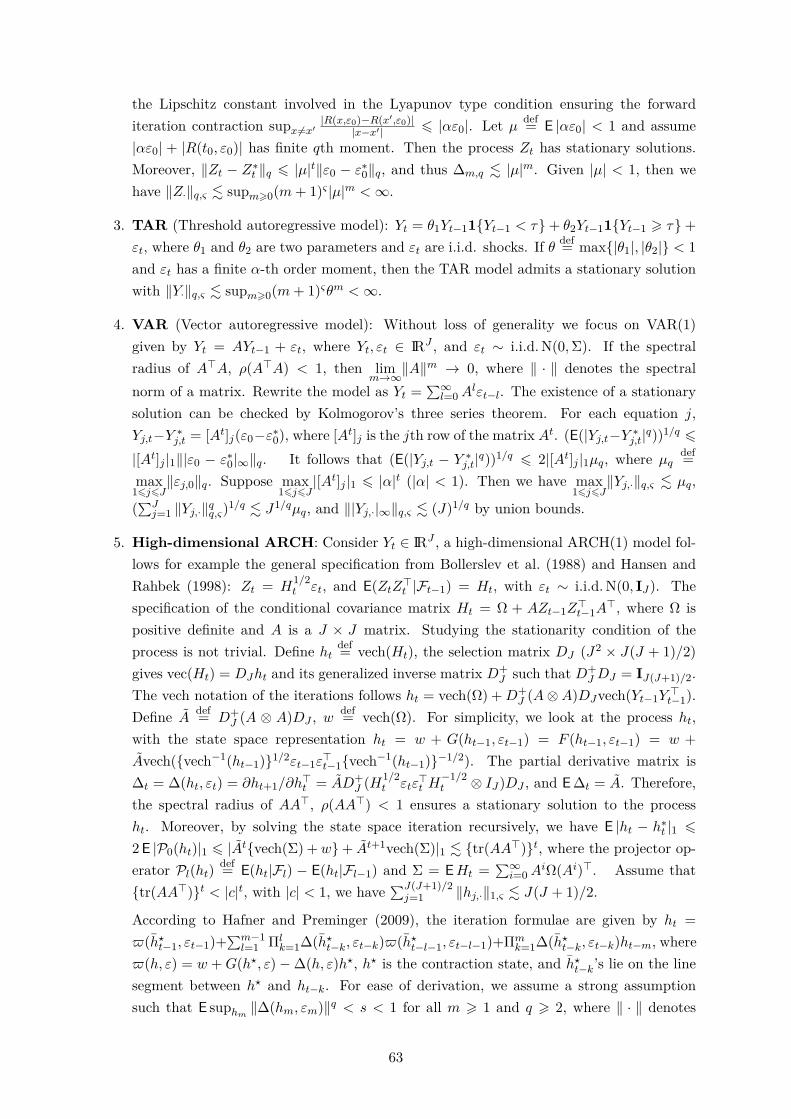
Comment 5.1. We allow for overlap in the elements in ξt and ηt, as long as the contempora-neous exogeneity condition E(Xjk,tεj,t) = 0 is satisfied. For example, consider the VAR(1)model: Yt = AYt−1 + εt, with Yt, εt ∈ IRJ , and suppose that Yt admits the representa-tion Yt =
∑∞l=0A
lεt−l with εt−l as measurable functions of ξ−∞, . . . , ξt−l. Thus Xjk,t =gjk(. . . , ξt−1) =
∑∞l=0[Al]kεt−1−l, where [Al]k is the kth row of the matrix Al, k = 1, . . . , J .
In this case no serial correlation in the innovations εt’s would be sufficient for E(Xjk,tεj,t) = 0.
Comment 5.2. We show in Theorem B.1 (see the supplementary materials) that the RE(A2) and RSE (A5) conditions can be implied by assumptions on the corresponding populationvariance-covariance matrix. This illustrates the feasibility of the RE/RSE assumption.
Lemma 5.1 (Prediction Performance Bound of Single Equation LASSO). Suppose (A1) and(A2) (with c = c+1
c−1 , c > 1), under the exact sparsity assumption (3.1) and given the eventλj > 2c
√n max
16k6K|Sjk/Ψjk| and another event which RE holds, then with probability 1−O(1), βj
obtained from (3.6) satisfy
|βj − β0j |j,pr 6 (1 + 1/c)
λj√sj
nκj(c)max
16k6KΨjk. (5.1)
In addition, if (A2) (with 2c) holds, then with probability 1− O(1),
|βj − β0j |1 6
(1 + 2c)√sjκj(2c)
|βj − β0j |j,pr. (5.2)
Lemma 5.1 follows Theorem 1 of Belloni and Chernozhukov (2013). As the proof is builton inequalities and for the case of dependent data (A1) they remain unchanged, we omit thedetailed proof here. To further characterize the rate of IC, we provide a tail probability for2c√n max
16k6K|Sjk/Ψjk| under the moment assumption (A3). In particular, the rate depends on
the dependence adjusted norm ‖Xjk,·εj,·‖q,ς .
Theorem 5.1. Under (A1) and (A3), we have
P(2c√n max
16k6K|Sjk/Ψjk| > r) 6C1$nnr
−qK∑k=1
‖Xjk,·εj,·‖qq,ςΨqjk
+ C2
K∑k=1
exp( −C3r
2Ψ2jk
n‖Xjk,·εj,·‖22,ς
),
(5.3)
where for ς > 1/2− 1/q (weak dependence case), $n = 1; for ς < 1/2− 1/q (strong dependencecase), $n = nq/2−1−ςq. C1, C2, C3 are constants depending on q and ς.
Comment 5.3. It can be seen in Theorem 5.1 that the rate of the dependence adjusted norm‖Xjk,·εj,·‖q,ς plays an important role in the tail probability for 2c
√n max
16k6K|Sjk/Ψjk|. Here we
discuss the rate under some special cases.
1. VAR(1): Consider the VAR(1) model given by Yt = AYt−1 + εt, where Yt, εt ∈ IRJ ,and εt ∼ i.i.d.N(0,Σ). In this case Xjk,t = Yj,t−1 and K = J . Suppose there exists astationary representation of the model as Yt =
maxj ‖εj,t‖q and [At−1]j is the jth row of the matrix At−1. Assume maxj |[At]j |1 6 |c|t
with |c| < 1 (a geometric decay rate). It follows that ‖Xjk,·εj,·‖q,ς = 2µ2q
1−|c| supm>0(m +1)ς∑∞t=m |c|t−1 6 (C/|c|)∨C(m∗+1)|c|m∗−1, where m∗ = (−ς/ log |c|−1)∨0 and C > 0
depends on µq. Moreover, to justify the geometric decay rate, we consider the example ofNetwork Autoregressive (NAR) model as in Zhu et al. (2017) with A = ρW , where W isa row-normalized adjacency matrix which is pre-specified to indicate the social networkconnectedness and ρ is the network parameter suggesting the strength of the networkeffects. In that case, assuming a geometric decay rate maxj |[At]j |1 6 |c|t with |c| < 1again gives similar results.
2. Spatial MA structure in εt: Consider the model Yj,t = X>j,tβj+εj,t, with εt = ρWεt+ηt,where W is a spatial weight matrix, ηt are i.i.d. and have finite qth moments µηq
def=maxj ‖ηj,t‖q. For simplicity, here we assume Xj,t and εj,t are independent. Supposethere exists a stationary representation of the error process given by εt =
1)|c|m∗−1, where m∗ = (−ς/ log |c|− 1)∨ 0 and C1, C2, C3 > 0 depend on µηq and ‖Xjk,t‖q.
3. General linear processes: To study more general spatial and temporal dependency,consider the model Yj,t = X>j,tβj + εj,t, with εt =
∑∞l=0A
lηt−l. Again ηt are i.i.d. andhave finite qth moments µηq
def= maxj ‖ηj,t‖q. If all the Al are diagonal matrices, thereis just temporal dependence, and if Al = 0 for l > 1 there exists only spatial depen-dence. Let atjk
def= [At]jk be the element on the jth row and kth column of At. As-sume
∑∞t=0
∑k |atjk| < ∞, Xj,t and εj,t to be independent. We have ‖Xjk,·εj,·‖q,ς 6
C1‖Xjk,·‖q,ς + C2 supm>0(m + 1)ς∑∞t=m
∑k |atjk|, where C1, C2 > 0 depend on µηq and
‖Xjk,t‖q. Moreover, we have ‖maxjk(Xjk,·εj,·)‖q,ς 6 ‖maxjkXjk,·‖q,ς‖maxj εj,·‖q,ς , andparticularly ‖|εt|∞‖q 6 ‖maxj
where the Rosenthal-Burkholder inequality is applied. Suppose that∑∞t=m(
∑k maxj |atjk|) .
J(m ∨ 1)−c, for some constant c > 0. If ς < c, we have ‖maxj εj,·‖q,ς 6 C3 supm>1(m +1)ς(m ∨ 1)−cJ
√log J 6 C3 supm>1(m+ 1)ς−cJ
√log J , where C3 > 0 depends on µηq .
To summarize, if the qth moments are bounded by constant, the dependence adjusted norm‖Xjk,·εj,·‖q,ς is also bounded in the first two examples where a geometric decay rate on thecoefficients is assumed; while in the case of general linear processes, it would depend on therate of
∑∞t=0
∑k |atjk|. In particular, suppose
∑∞t=m
∑k |atjk| . (m ∨ 1)−c for c > 0. If c > ς,
‖Xjk,·εj,·‖q,ς is bounded (assume ‖Xjk,·‖q,ς is bounded).
Under the choice (IC) λ0j (1 − α) is given by the (1 − α) quantile of 2c
√n max
16k6K|Sjk/Ψjk|,
combining the results of Lemma 5.1 and Theorem 5.1 we can get the bounds for λ0j (1− α) and
further obtain the oracle inequalities as in Corollary 5.1.
16
Corollary 5.1 (Bounds for λ0j (1 − α) and Oracle Inequalities under IC). Under (A1)-(A3),
given λ0j (1− α) satisfying
λ0j (1− α) . max
16k6K
‖Xjk,·εj,·‖2,ς
√n log(K/α) ∨ ‖Xjk,·εj,·‖q,ς(n$nK/α)1/q
, (5.4)
and the exact sparsity assumption (3.1), then βj obtained from (3.6) under IC satisfies
|βj − β0j |j,pr .
√sj
κj(c)max
16k6KΨjk
‖Xjk,·εj,·‖2,ς
√log(K/α)√
n∨ ‖Xjk,·εj,·‖q,ςn1/q−1($nK/α)1/q
,
(5.5)with probability 1 − α − O(1), where for ς > 1/2 − 1/q (weak dependence case), $n = 1; forς < 1/2− 1/q (strong dependence case), $n = nq/2−1−ςq.
Comment 5.4. The Nagaev type of inequality in (5.3) has two terms, namely an exponentialterm and a polynomial term. It should be noted that if the polynomial term dominates, theabove bound does not allow for ultra high dimension of K. Basically, we only allow for apolynomial rate K = O(nc), and the rate of K interplays with the dependence adjusted norm‖Xjk,·εj,·‖q,ς . In particular, to make sure that the estimators are consistent (i.e. the errorbounds tend to zero for sufficiently large n), for example, we need c < q − 1 − υq/2 − dq, ifthere exists q to guarantee ‖Xjk,·εj,·‖q,ς = O(nd) and 0 < υ < 1 such that sj = O(nυ).
We now discuss the case of sub-Gaussian tail or sub-exponential tail, which is mostly assumedin the literature.
Comment 5.5. Suppose a stronger exponential moment condition is satisfied,
‖Xjk,·εj,·‖ψν ,ς = supq>2
q−ν‖Xjk,·εj,·‖q,ς <∞, (5.6)
where ‖Xjk,·εj,·‖ψν ,ς is interpreted as the dependence adjusted sub-exponential (ν = 2) orsub-Gaussian (ν = 1) norm. Consider the special case of VAR(1). As shown above, we have‖Xjk,tεj,t−X∗jk,tε∗j,t‖q 6 2|[At−1]j |1µ2
q . In particular, it is known that µq . q for sub-exponentialvariables and µq .
√q for sub-Gaussian variables. Let ν = 2 and ν = 1 for the two cases
respectively, ‖Xjk,·εj,·‖ψν ,ς . (m∗ + 1)|c|m∗−1. Then applying the exponential tail bounds asin Lemma B.3 in the supplementary material, we arrive at the following error bounds withprobability 1− α− O(1),
|βj − β0j |j,pr .
√sj
κj(c)max
16k6KΨjk‖Xjk,·εj,·‖ψν ,0
log(K/α)1/γ√n
, γ = 2/(2ν + 1), (5.7)
as λ0j (1 − α) .
√n(logK)1/γ max
16k6K‖Xjk,·εj,·‖ψν ,0. The bound (5.7) works with ultra-high di-
mensional rate exp(nrγ) (r < 1) of K as only the exponential term shows in the inequality. Inparticular, suppose sj = O(nυ), and ‖Xjk,·εj,·‖ψν ,0 = O(nd), then r+ d+ υ/2 < 1/2 is requiredto ensure the consistency.
17
5.2 Gaussian Approximation for Dependent Data
Now we look at the validity of the choice of Qj(1−α), which relies on a Gaussian approximationtheorem. First we define the Kolmogorov distance between any two K-dim random vectors.
Definition 5.2. Let X = (X1, · · · , XK)> ∈ IRK , Y = (Y1, · · · , YK)> ∈ IRK . The Kolmogorovdistance between X and Y is defined as
ρ(X,Y ) = supr>0
∣∣P(|X|∞ > r)− P(|Y |∞ > r)∣∣.
For each single equation j, aggregate the dependence adjusted norm over k = 1, . . . ,K:
‖|Xj,·|∞‖q,ςdef= sup
m>0(m+ 1)ς
∞∑t=m
δq,j,t, δq,j,tdef= ‖|Xj,t −X∗j,t|∞‖q, (5.8)
where q > 1 and ς > 0. Moreover, define the following quantities
Φj,q,ςdef= 2 max
16k6K‖Xjk,·‖q,ς‖εj,·‖q,ς , Γj,q,ς
def= 2‖εj,·‖q,ς( K∑k=1‖Xjk,·‖q/2q,ς
)2/q
Θj,q,ςdef= Γj,q,ς ∧
2‖|Xj,·|∞‖q,ς‖εj,·‖q,ς(logK)3/2. (5.9)
It is worth noting that the norm ‖|Xj,·|∞‖q,ς is a kind of aggregated dependence adjustednorm for a vector of processes in comparison to the dependence adjusted norm for a univariateprocess as in Definition 5.1.
Some additional assumptions are required. Define L1,j = Φj,4,ςΦj,4,0(logK)21/ς , W1,j =(Φ6
The assumptions impose mild restrictions on the dependency structure of covariates anderror terms. They include a wide class of potential correlation and heterogeneity (includingconditional heteroscedasticity), with possible allowance of the lagged dependent variables. Twoexamples of large VAR and ARCH for high-dimensional time series can be found in AppendixC.2 in the supplementary materials.
Comment 5.6. [Admissible Dimension Rates by the Conditions for Gaussian Approximation]As discussed in Zhang and Wu (2017a), consider the case with Θj,2q,ς = O(K1/q) and Φj,2q,ς =O(1), where ς > 1/2− 1/q. Then Θj,2q,ςn
1/q−1/2log(Kn)3/2 → 0 becomes Klog(nK)3q/2 =O(nq/2−1), which implies that L1 max(W1,W2) = O(1) min(N1, N2). This means with (A4), thedimension K has to satisfy the condition K(logK)3q/2 = O(nq/2−1).
Theorem 5.2 (Gaussian Approximation Results for Dependent Data). Under (A1) and (A3)-(A4), for each j = 1, . . . , J assume that there exists a constant cj > 0 such that min
16k6Kavar(Sjk) >
18
cj, then we haveρ(D−1j Sj·, D
−1j Zj
)→ 0, as n→∞, (5.10)
where Zj ∼ N(0,Σj), Σj is the K ×K long-run variance-covariance matrix of Xj,tεj,t, and Dj
is a diagonal matrix with the square root of the diagonal elements of Σj, namely
∞∑`=−∞
E(Xjk,tXjk,(t−`)εj,tεj,(t−`))1/2
=√
avar(Sjk), for k = 1, . . . ,K.
Comment 5.7. The conclusion in Theorem 5.2 can be held with stronger tail assumptions,following Theorem 5.2 in Zhang and Wu (2017a).
Theorem 5.2 justifies the choice of λj and Qj(1−α), which leads to the following corollary:
Corollary 5.2. Under the conditions of Theorem 5.2, for each j we have
supα∈(0,1)
∣∣P max16k6K
2c√n|Sjk/Ψjk| > Qj(1− α) − α
∣∣→ 0, as n→∞. (5.11)
It is worth noting that in practice the variance involved in the Gaussian approximation in 5.2is not known; we shall discuss how we estimate the variance and also the validity of the Gaussianapproximation result with an estimated variance. Given the realization Xj,1εj,1, . . . , Xj,nεj,n,we propose to estimate the K ×K long-run variance-covariance matrix Σj for j = 1, . . . , J asfollows, given EXj,tεj,t = 0, and consider:
Σj = 1bnln
ln∑i=1
( ibn∑l=(i−1)bn+1
Xj,lεj,l)( ibn∑l=(i−1)bn+1
Xj,lεj,l)>. (5.12)
Moreover, the following corollary ensures that the Gaussian approximation results still hold ifwe use the estimate in (5.12).
Corollary 5.3. Let the conditions of Theorem 5.2 hold, and assume Φj,2q,ς < ∞ with q > 4,bn = O(nη) for some 0 < η < 1. Let Fς = n, for ς > 1 − 2/q; Fς = lnb
n or 1) for ς = 1 (resp. ς < 1or ς > 1). Then for each j we have
ρ(D−1j Sj·, D
−1j Zj
)→ 0, as n→∞, (5.13)
where Dj = diag(Σj)1/2.
It should be noted that given the Gaussian approximation results in Theorem 5.2, we canhave a refined bound for λ0
j (1− α) and also the oracle inequalities under IC.
Corollary 5.4 (Bounds for λ0j (1−α) and Oracle Inequalities under IC with Gaussian Approx-
imation Results). Under the conditions of Theorem 5.2 together with (A2), let 2(logK)−1/2 +ρ(D−1
j Sj·, D−1j Zj) = O(α) and Zα > 2c
√n logK, where c is no less than the c in the definition
19
of λ0j (1− α), then we have λ0
j (1− α) satisfying
λ0j (1− α) 6 Zα, (5.14)
and given the exact sparsity assumption (3.1), then βj obtained from (3.6) under IC satisfies
|βj − β0j |j,pr .
√sj
κj(c)max
16k6KΨjk
√logK√n
, (5.15)
with probability 1− α− O(1).
We note that the allowed dimension K is still of polynominal rate restricted by (A4).
5.3 Multiplier Block Bootstrap Procedure
In this subsection, we discuss how Λj(1 − α) is attainable via block bootstrap. The data overt = 1, . . . , n are divided into ln blocks with the same number of observations bn, n = bnln
(without loss of generality), where bn, ln ∈ Z.Recall that Λj(1 − α) = 2c
√nq
[B]j,(1−α), q
[B]j,(1−α) is the (1 − α) quantile of max
16k6K|Z [B]jk /Ψjk|,
where Z [B]jk are defined as
Z[B]jk = 1√
n
ln∑i=1
ej,i
ibn∑l=(i−1)bn+1
εj,lXjk,l, (5.16)
and ej,i are i.i.d. N(0, 1) random variables independent of X and ε.In fact, the above construction relies on knowing the true residuals εj,t. In practice, one
needs to pre-estimate them using a conservative choice of penalty levels and loadings. The issueof generated errors can be dealt with using a similar argument as in the proof of Corollary 5.3.
Theorem 5.3 (Validity of Multiplier Block Bootstrap Method). Under (A1) and (A3), andassume Φj,2q,ς <∞ with q > 4, bn = O(nη) for some 0 < η < 1 (the detailed rate is calculatedin (B.2) in the supplementary materials), then we have
supα∈(0,1)
∣∣P ( max16k6K
|Sjk/Ψjk| > q[B]j,(1−α)
)− α
∣∣→ 0, as n→∞. (5.17)
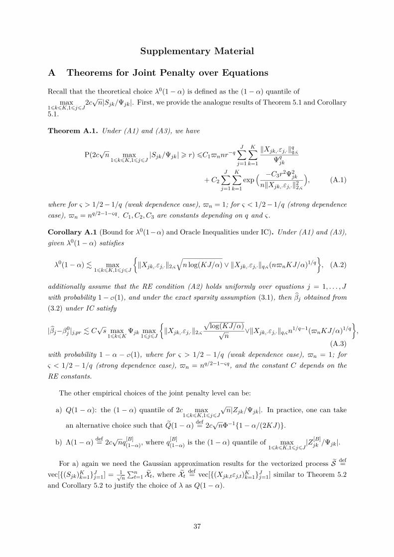
5.4 Joint Penalty over Equations
Recall that the theoretical choice λ0(1−α) is defined as the (1−α) quantile of max16k6K,16j6J
2c√n|Sjk/Ψjk|.
The empirical choices of the joint penalty level can be:
a) Q(1 − α): the (1 − α) quantile of 2c max16k6K,16j6J
√n|Zjk/Ψjk|. In practice, one can take
an alternative choice such that Q(1− α) def= 2c√nΦ−11− α/(2KJ).
b) Λ(1− α) def= 2c√nq
[B](1−α), where q
[B](1−α) is the (1− α) quantile of max
16k6K,16j6J|Z [B]jk /Ψjk|.
Section A in the supplementary material provides the main theorems for joint equationestimation. In particular, the dimension along k = 1, . . . ,K and j = 1, . . . , J will be considered
20
together by vectorization, resulting in the dimension of KJ . Following the results for the singleequation (where j is fixed), we generalize the theorems above to multiple equations case bychanging the dimension from K to KJ , see Section A in the Appendix for more details.
5.5 Post-Model Selection Estimation
LASSO estimation is known to be biased especially for large coefficients. Therefore, a post-selection step helps to reduce the bias by running an OLS as a second step on the selectedcovariates in the first step. In particular, we consider the 2-step OLS post-LASSO estimator:
i) `1-penalized regression (LASSO selection)
βj = arg minβ∈IRK
1n
n∑t=1
(Yj,t −X>j,tβ)2 + λ
n
K∑k=1|βjk|Ψjk, (5.18)
where λ is the joint penalty level.
ii) We run the post-selection regression (OLS estimation)
β[P ]j = arg min
β∈IRK 1n
n∑t=1
(Yj,t −X>j,tβ)2 : βk = 0, k /∈ Tj, (5.19)
where Tjdef= supp(βj) = k ∈ 1, . . . ,K : βjk 6= 0.
To provide the prediction performance bounds for the OLS post-LASSO estimators, we needthe following restricted sparse eigenvalue (RSE) condition:
(A5) Restricted sparse eigenvalue (RSE): given p < n, for δ ∈ IRK , with probability 1− O(1),
κj(p)2 def= min|δTc
j|06p,δ 6=0
|δ|2j,pr|δ|22
> 0, φj(p)def= max|δTc
j|06p,δ 6=0
|δ|2j,pr|δ|22
> 0.
Here p denotes the restriction on the length of the active set of T cj . When Tj = ∅, (A5) is
reduced to the standard sparse eigenvalue condition. Moreover, let µj(p)def=√φj(p)κj(p) , and denote
by pjdef= |Tj\Tj | the number of components outside Tj
def= supp(β0j ) = k ∈ 1, . . . ,K : β0
jk 6= 0selected by LASSO in the first step.
The performance bounds for the OLS post-LASSO estimator are shown in Theorem A.4 inthe supplementary materials.
5.6 Simultaneous Inference
This subsection develops theory corresponding to Section 4. A key Bahadur representationwhich linearize the estimator for a proper application of the central limit theorem for inferenceis provided.
21
Recall that for each j = 1, . . . , J , the following model is considered
E(Xjk,t−X>j(−k),tγj(−k))2, and let Fεj denote the distributionfunction of εj,t. In this subsection, we show the validity of the joint confidence region forsimultaneous inference on H0 : β0
jk = 0, ∀(j, k) ∈ G, with |G| =∑Jj=1 pj . In particular, for
j = 1, . . . , J , β0jk (k = 1, . . . , pj) are the target parameters. Theoretically, we formulate the
estimation as a general Z-estimation problem, with the leading examples as the LAD/LS cases.Nevertheless, it can also include a more general class of loss functions.
For each (j, k) ∈ G, we define the score function as ψjkZj,t, βjk, hjk(Xj(−k),t), whereZj,t
def= (Yj,t, X>j,t)> and the vector-valued function hjk(·) is a measurable map from IRK−1
to IRM (M is fixed). In particular, in our linear regression case we have hjk(Xj(−k),t) =(X>j(−k),tβj(−k), X
>j(−k),tγj(−k))>, and for the LAD regression ψjkZj,t, βjk, hjk(Xj(−k),t) = 1/2−
1(Yj,t 6 Xjk,tβjk +X>j(−k),tβj(−k))(Xjk,t −X>j(−k),tγj(−k)).Assume that there exists s = sn > 1 such that |β0
j(−k)|0 6 s, |γ0j(−k)|0 6 s, for each (j, k) ∈ G.
Moreover, we assume that the nuisance function h0jk = (h0
jk,m)Mm=1 admits a sparse estimatorhjk = (hjk,m)Mm=1 of the form
where gndef= log(e|G|)1/2 and Bjk is defined in (C2).
We now lay out the following conditions needed in this section, which are assumed to holduniformly over (j, k) ∈ G.
(C1) Orthogonality condition:
E[∂h Eψjk(Zj,t, β0
jk, h)|Xj(−k),t∣∣h=h0
jk(Xj(−k),t)
h(Xj(−k),t)]
= 0, (5.22)
for any h ∈ Hjk ∪ h0jk, where Hjk is defined in (C5).
22
(C2) The true parameter β0jk satisfies (5.21). Let Bjk be a fixed and closed interval and Bjk be
a possibly stochastic interval such that with probability 1−O(1), [β0jk±c1rn] ⊂ Bjk ⊂ Bjk,
where rndef= n−1/2(log an)1/2 max
(j,k)∈G‖ψ0
jk,·‖2,ς + n−1rς(log an)3/2∥∥ max(j,k)∈G
|ψ0jk,·|
∥∥q,ς, rn . ρn
(ρn is defined in (C5)), andef= max(JK, n, e), and ψ0
jk,tdef= ψjkZj,t, β0
jk, h0jk(Xj(−k),t).
rς = n1/q for ς > 1/2− 1/q and rς = n1/2−ς for ς < 1/2− 1/q.
(C3) Properties of the score function: the map (β, h) 7→ Eψjk(Zj,t, β, h)|Xj(−k),t is twice con-tinuously differentiable, and for every ϑ ∈ β, h1, . . . , hM,E[supβ∈Bjk |∂ϑ Eψjk(Zj,t, β, h0
jk(Xj(−k),t)|Xj(−k),t|2] 6 C1; moreover, there exist mea-surable functions `1(·), `2(·), constants L1n, L2n > 1, υ > 0 and a cube Tjk(Xj(−k),t) =×Mm=1Tjk,m(Xj(−k),t) in IRM with center h0
jk(Xj(−k),t) such that for every ϑ, ϑ′ ∈ β, h1, . . . , hMwe have sup(β,h)∈Bjk×Tjk(Xj(−k),t) |∂ϑ∂ϑ′ Eψjk(Zj,t, β, h)|Xj(−k),t| 6 `1(Xj(−k),t),E|`1(Xj(−k),t)|4 6 L1n, and for every β, β′ ∈ Bjk, h, h′ ∈ Tjk(Xj(−k),t) we have E[ψjk(Zj,t, β, h)−ψjk(Zj,t, β′, h′)2|Xj(−k),t] 6 `2(Xj(−k),t)(|β−β′|υ+|h−h′|υ2), and E|`2(Xj(−k),t)|4 6 L2n.
(C5) Properties of the nuisance function: with probability 1 − O(1), hjk ∈ Hjk, where Hjk =×Mm=1Hjk,m and each Hjk,m being the class of functions of the form hjk,m(Xj(−k),t) =X>j(−k),tθjk,m, |θjk,m|0 6 s, hjk,m ∈ Tjk,m. There exists sequence of constants ρn ↓ 0 suchthat E[hjk,m(Xj(−k),t)− h0
jk,m(Xj(−k),t)2] . ρ2n.
(C6) The class of functions Fjk = z 7→ ψjkz, β, h(xj(−k)) : β ∈ Bjk, h ∈ Hjk ∪ h0jk (z
is a random vector taking values in a Borel subset of a Euclidean space which containsthe vectors xj(−k) as subvectors) is pointwise measurable and has measurable envelopeFjk > sup
f∈Fjk|f |, such that F = max
(j,k)∈GFjk satisfies EF q(z) <∞ for some q > 4.
(C7) The second-order moments of scores are bounded away from zero: ωjk = E( 1√n
O(ρn). F ′ = z 7→ ψjkz, β, h(xj(−k)) : (j, k) ∈ G, β ∈ Bjk, h ∈ Hjk ∪ h0jk with
F ′ = supf∈F ′|f |.
(C9) Let BhΦ = max
m∈1,2Φhm,2,ς , Bh
Ω = maxm∈1,2
Ωhm,q,ς , B
′hΦ = max
m∈1,2Φ′hm,2,ς , and B
′hΩ = max
m∈1,2Ω′hm,q,ς
(see (B.9), (B.10) and (B.15) in the supplementary for the definitions of Φhm,2,ς , Ωh
m,q,ς ,Φβ
2,ς , Ωβq,ς , Φ′hm,2,ς , Ω′hm,q,ς , Φ
′β2,ς , Ω′βq,ς). The following restrictions are assumed:
sρn(log an)1/2BhΦ + n−1/2rςρns
2(log an)3/2BhΩ = O(g−1
n ),
ρn(s log an)1/2Φβ2,ς + n−1/2rςρn(s log an)3/2Ωβ
q,ς = O(g−1n ),
23
B′hΦ ρns
1/2 = O(maxf∈F ′
‖f(zt)‖2), B′hΩ ρns1/2 = O(‖F ′(zt)‖q),
Φ′β2,ςρn = O(max
f∈F ′‖f(zt)‖2), Ω′βq,ςρn = O(‖F ′(zt)‖q).
(C9’) Consider the stronger exponential moment condition as in (5.6) and corresponding to(C5), assume that E[hjk,m(Xj(−k),t) − h0
jk,m(Xj(−k),t)2] . (ρen)2. Recall the definitionsof Φh
m,ψν ,0, Φβψν ,0, Φ′hm,ψν ,0, Φ
′βψν ,0 in (B.17) and (B.20) in the supplementary. The following
restrictions are assumed:
n−1/2(log an)1/γ max(j,k)∈G
‖ψ0jk,·‖ψν ,0 . rn,
(s log an)1/γ[ρen,υ ∨ ρen(s1/2 maxm∈1,2
Φhm,ψν ,0) ∨ Φβ
ψν ,0]
= O(g−1n ),
n−1/2(s log an)1/γ maxf∈F ′
‖f(z·)‖ψν ,0 = O(ρen),
ρen(s1/2 maxm∈1,2
Φ′hm,ψν ,0) ∨ Φ′βψν ,0 = O(max
f∈F ′‖f(z·)‖ψν ,0),
in particular, for the mean regression case ρen,υ = ρens and ρen,υ = √ρen for the medianregression case.
(C10) The density of error fεj (·) is continuously differentiable and both of fεj (·) and f ′εj (·) arebounded from the above.
Conditions (C1)-(C4) and (C7) assume mild restrictions on the Z-estimation problems. Theyinclude the LAD-based regression (used in Algorithm 2) with nonsmooth score function. Con-ditions (C2) and (C8) imply that max
(j,k)∈G‖ψ0
jk,·‖2,ς . s1/2maxf∈F ′‖f(zt)‖2 and
∥∥ max(j,k)∈G
|ψ0jk,·|
∥∥q,ς
.
s3/2‖F ′(zt)‖q. In (C5), we suppose that the nuisance parameters have estimators with goodsparsity and convergence rate properties. As discussed in previous sections, given the idealchoice of the tuning parameter, the oracle inequalities provided in Corollary 5.1 ensuresthat our proposed algorithms can produce the estimator of the form |β[1]
j(−k) − β0j(−k)|j,pr .
√s log(an)/n ∨ n1/q−1($nan)1/q max
16k6K‖Xjk,·εj,·‖q,ς , where for ς > 1/2 − 1/q (weak depen-
dence case), $n = 1; for ς < 1/2 − 1/q (strong dependence case), $n = nq/2−1−ςq. Themoments of the envelopes are assumed to be finite in (C6).
Comment 5.8. [Discussion on the dimension growth rates] Consider the special case of VAR(1)model. Following the discussion in Comment 5.3, given a geometric decay rate, we haveL2n, B
hΦ, B
′hΦ ,Φ
β2,ς ,Φ
′β2,ς ,max
f∈F ′‖f(zt)‖2, max
(j,k)∈G
∥∥|ψ0jk,·|
∥∥2,ς . Mn, where Mn only depends on the
2q-th moments of εt and ς. Moreover, suppose these quantities are bounded by constant and letdn
def= (|G| ∨ J), we have BhΩ, B
′hΩ . d
1/qn (1 ∨ s1/2ρn), Ωβ
q,ς ,Ω′βq,ς . d
1/qn s1/2ρn for mean regression
case, and BhΩ, B
′hΩ . d
3/(4q)n (1 ∨ s1/2ρn), Ωβ
q,ς ,Ω′βq,ς . d
1/(2q)n s1/2ρn for the median regression.
Moreover, ‖F (zt)‖q, ‖F ′(zt)‖q . d1/qn (1 ∨ ρn),
∥∥ max(j,k)∈G
|ψ0jk,·|
∥∥q,ς
. d1/qn (1 ∨ ρn). The detailed
derivation of these rates can be found in the Comment B.3 in the supplementary. Inserting
for the smooth and non-smooth cases respectively. As a result, we only allow the dimension(|G| ∨ J) is of polynomial order with respect to n if q is not tending to infinity. In particu-lar, under the case of ς > 1/2 and q = ∞, the required rate reduces to n−1/2s2(log an)3/2 +n−1s3(log an)5/2 + n−1/2s3/2(log an)2 = O(1) or n−1/4s3/4(log an)5/4 + n−1/2s5/4(log an)7/4 +n−1/2s3/2(log an)2 = O(1), respectively. In the ideal case where we have weak dependency, thedimension growth rates are slightly slower than the i.i.d. case as in Belloni et al. (2015b) (i.e.,s2 log a3
n = O(n) or s3 log a5n = O(n) for the smooth or non-smooth case, respectively), as we
apply a different way to bound the dependence adjusted norm in the concentration inequality.More generally, suppose max
L2n, B
hΦ, B
′hΦ ,Φ
β2,ς ,Φ
′β2,ς ,max
f∈F ′‖f(zt)‖2, max
(j,k)∈G
∥∥|ψ0jk,·|
∥∥2,ς
= O(nk1),
and maxBh
Ω, B′hΩ ,Ωβ
q,ς ,Ω′βq,ς , ‖F (zt)‖q, ‖F ′(zt)‖q,
∥∥ max(j,k)∈G
|ψ0jk,·|
∥∥q,ς
= O(nk2), with 0 6 k1 6 k2,
and let s = O(nv), log an = O(nr). Then (C8) and (C9) imply that
r < max1− 4v − 2k1
3 ,− 25q + 2− 6v − 2k2
5 ,− 12q + 1− 3v − 2k2
4
, if ς > 1/2− 1/q,
r < max1− 4v − 2k1
3 ,2ς + 1− 6v − 2k2
5 ,2ς − 3v − 2k2
4
, if ς < 1/2− 1/q,
and
r < max1− 3v − 4k1
5 ,− 27q + 2− 5v − 2k2
7 ,− 12q + 1− 3v − 2k2
4
, if ς > 1/2− 1/q,
r < max1− 3v − 4k1
3 ,2ς + 1− 5v − 2k2
7 ,2ς − 3v − 2k2
4
, if ς < 1/2− 1/q,
for the smooth and non-smooth cases.
Theorem 5.4. [Uniform Bahadur Representation] Under conditions (A1)-(A4) and (C1)-(C10), with probability 1− O(1), we have
max(j,k)∈G
|n1/2σ−1jk (βjk − β0
jk) + n−1/2σ−1jk φ
−1jk
n∑t=1
ψ0jk,t| = O(g−1
n ), as n→∞, (5.23)
where σ2jk
def= φ−2jk ωjk, ωjk
def= E( 1√n
∑nt=1 ψ
0jk,t)2.
Comment 5.9. The same conclusion as in Thereom 5.4 can be drawn with assuming strongerexponential moment conditions in (5.6) and using (C9’) instead of (C6), (C8) and (C9). Thisis implied by Lemma B.8, B.9 and B.10 in the supplementary material.
We now discuss the rates implication under (C9’). Suppose all the dependence adjustednorms are bounded by constant with an appropriately chosen ν, the restrictions in (C9’) would
25
imply n−1/2(log an)2/γ+1/2s2/γ+1 = O(1) for the case of smooth score, andn−1/4(log an)3/(2γ)s3/(2γ)+1/2 = O(1) for the non-smooth case, where γ = 2/(2ν + 1). Forexample, when ν = 1/2, γ = 1 the required rates would be s6 log5 an = O(n) and s6 log8 an =O(n) for the smooth and non-smooth cases respectively.
The results in Theorem 5.4 imply the asymptotic normality of the proposed estimator byAlgorithm 1 and 2 by applying central limit theorems and Gaussian Approximation.
Corollary 5.5. Under conditions (A1)-(A4) and (C10), for any (j, k) ∈ G the estimatorsobtained by Algorithm 1 and 2 satisfy
σ−1jk n
1/2(β[2]jk − β
0jk)
L→ N(0, 1).
Theorem 5.5. [Uniform-Dimensional Central Limit Theorem] Under the same conditions asin Theorem 5.4, assume that ‖ψ0
jk,·‖2,ς <∞, we have
σ−1jk n
1/2(βjk − β0jk)
L→ N(0, 1),
uniformly over (j, k) ∈ G.
Consider the vector ζtdef= vec(ζjk,t)(j,k)∈G, ζjk,t
def= −σ−1jk φ
−1j,kψ
0jk,t, and define the aggre-
gated dependence adjusted norm as follows:
‖ζ·‖q,ςdef= sup
m>0(m+ 1)ς
∞∑t=m‖|ζt − ζ∗t |∞‖q, (5.24)
where q > 1, and ς > 0. Moreover, define the following quantities
Φζq,ς
def= max(j,k)∈G
‖ζjk,·‖q,ς , Γζq,ςdef=( ∑
(j,k)∈G‖ζjk,·‖qq,ς
)1/q,
Θζq,ς
def= Γζq,ς ∧‖ζ·‖q,ς(log |G|)3/2. (5.25)
Define Lζ1 = Φζ2,ςΦ
ζ2,0(log |G|)21/ς ,W ζ
1 = (Φζ3,0)6+(Φζ
4,0)4log(|G|n)7,W ζ2 = (Φζ
2,ς)2log(|G|n)4,W ζ
3 = [n−ςlog(|G|n)3/2Θζq,ς ]1/(1/2−ς−1/q), N ζ
1 = (n/ log |G|)q/2(Θζq,ς)q, N
ζ2 = n(log |G|)−2(Φζ
2,ς)−2,N ζ
3 = n1/2(log |G|)−1/2(Θζq,ς)1/(1/2−ς).
(A6) i) (weak dependency case) Given Θζq,ς < ∞ with q > 2 and ς > 1/2 − 1/q, then
Θζq,ςn
1/q−1/2log(|G|n)3/2 → 0 and Lζ1 max(W ζ1 ,W
ζ2 ) = O(1) min(N ζ
1 , Nζ2 ).
ii) (strong dependency case) Given 0 < ς < 1/2 − 1/q, then Θζq,ς(log |G|)1/2 = O(nς) and
Lζ1 max(W ζ1 ,W
ζ2 ,W
ζ3 ) = O(1) min(N ζ
2 , Nζ3 ).
Corollary 5.6 (Consistency of the Bootstrap Confidence Interval). Under (A6) and the sameconditions as in Theorem 5.4, for each (j, k) ∈ G assume that there exists a constant c > 0 suchthat min
where Zjk’s are the standard normal random variables and σjk is a consistent estimator of σjk.
Following Theorem 5.4, a joint confidence region and the corresponding confidence intervalfor each component can be constructed via a block bootstrap method. In particular, the boot-strap statistic are defined by 1√
n
∑lni=1 ej,i
∑ibnl=(i−1)bn+1 ζjk,l, where ej,i’s are independent and
identically distributed draws of standard normal random variables and are independent withrespect to the data sample (Zj,t)Jj=1. Recall that ζjk,t are pre-estimators with a certain rangeof accuracy.
Corollary 5.7 (Validity of Multiplier Bootstrap). Under the same conditions as in Theorem5.4, assume Φζ
q,ς <∞ with q > 4, bn = O(nη) for some 0 < η < 1 (the detailed rate is specifiedin (B.27)), we have
], and q∗(1 − α) is the (1 − α) conditional quantile
of max(j,k)∈G
1√n|∑lni=1 ej,i
∑ibnl=(i−1)bn+1 ζjk,l|.
6 Simulation Study
In this section, we illustrate the performance of our proposed methodology under differentsimulation scenarios. The first part concerns the performance of the jointly selected penaltylevel over equations, and the second part discusses the simultaneous inference.
6.1 Estimation with a Jointly Selected Penalty Level
where Xt ∈ IRK . We generate Xt independently from N(0,Σ), where Σk1,k2 = γ|k1−k2|, γ = 0.5,εj,t
i.i.d.∼ N(0, 1). The coefficient vectors βj are assumed to be sparse. In particular, we dividethe indices 1, . . . ,K evenly into blocks with fixed block size 5. β0
jk = 10 if k and j belong tothe same block and 0 otherwise.
We take n = 100, # of bootstrap replications = 5000. We set J,K = 50, 100 and 150.The prediction norm |βj − β0
j |j,pr and the Euclidean norm |βj − β0j |2 ratios are presented in
Table 6.1. The ratios measure the relative difference between the results using the penalty leveldetermined from the equation-by-equation case and from the joint equation case (λj and λ areselected by the multiplier bootstrap procedure). In particular, a ratio smaller than 1 indicatesa better performance of using the jointly selected penalty level.
27
J = K = 50 J = K = 100 J = K = 150Prediction norm
Mean 0.9634 0.9474 0.9347Median 0.9695 0.9516 0.9371Std. 0.0323 0.0272 0.0254
Table 6.1: Prediction norm and Euclidean norm ratios (overall λ relative to equation-by-equation λj ’s, average over equations). Results (mean, median and standard deviation) arecomputed over 1000 replications.
It is evident from Table 6.1 that the proposed estimation procedure delivers much betterperformance in terms of the two measures. In particular, the superiority tends to be moreevident (more than 10%) with higher dimension of the covariates and more equations.
Still consider the system of regression equations as in (6.1), but here we generate the datawith dependency by following the Appendix D in Zhang and Wu (2017b). In particular, assumethe linear process such that Xt =
∑∞`=0A`ξt−`, with A` = (` + 1)−ρ−1M`, where M` are
independently drawn from Ginibre matrices, i.e. all the entries of M` are i.i.d. N(0, 1), and inpractice the sum is truncated to
∑1000`=0 . We set ρ to be 1.0 for the weaker dependence and 0.1
for the stronger dependence cases respectively. Let ξk,t = ek,t(0.8e2k,t−1 + 0.2)1/2 where ek,t are
i.i.d. distributed as t(d)/√d/(d− 2) and t(d) is the Student’s t with degree of freedom d (take
d = 8 for example). εt are generated by following the same fashion independently.We take n = 100, # of bootstrap replications = 5000, J,K = 50, 100 and 150. Based on
bias-variance tradeoff, several approaches were suggested to determine the optimal choice of bnfor univariate case. Concerning the high-dimensional case, we propose to take the one whichgives the lowest prediction norm as the optimal choice. Below we report the average predictionnorm J−1∑J
j=1 |βj −β0j |j,pr with several block sizes bn under different settings and the minimal
ones are in bold.
ρ = 0.1 (stronger dependency) ρ = 1.0 (weaker dependency)J = K = 50 J = K = 100 J = K = 150 J = K = 50 J = K = 100 J = K = 150
Table 6.2: The prediction norm (average over equations) using several choices of bn. Resultsare computed over 1000 simulations.
From Table 6.2, it is apparent that a larger block size is required for the stronger dependency
28
case. Moreover, the choice also depends on the dimensionality, which is more evident forrelatively weaker dependent data. We note that when J = K = 50, ρ = 1.0 the ordinarymultiplier bootstrap (with bn = 1) produces 2.1003 as the average prediction norm, thereforewe suggest bn = 2 for this case.
The prediction norm |βj−β0j |j,pr and the Euclidean norm |βj−β0
j |2 ratios (using the optimalbn suggested in Table 6.2 for each case correspondingly) are presented in Table 6.3. Again wereport the results with the jointly estimated λ (selected by multiplier block bootstrap) relativeto using the single equation λj ’s (selected by the multiplier bootstrap).
ρ = 0.1 (stronger dependency) ρ = 1.0 (weaker dependency)J = K = 50 J = K = 100 J = K = 150 J = K = 50 J = K = 100 J = K = 150
Table 6.3: Prediction norm and Euclidean norm ratios (overall λ relative to equation-by-equation λj ’s, average over equations). Results (mean, median and standard deviation) arecomputed over 1000 replications.
The results show that the coefficient estimation performance measured by both the predic-tion norm and the Euclidean norm is in favor of the joint penalty level with multiplier blockbootstrap approach. The results are robust over different dimension cases with stronger orweaker dependency.
6.2 Simultaneous Inference
In this subsection we consider the following regression model for the purpose of simultaneousinference on the parameters within a system of equations
Yj,t = dj,tα0j +X>t β
0j + εj,t, dj,t = X>t θ
0j + vj,t, t = 1, . . . , n, j = 1, . . . , J, (6.2)
where α0j = α0 for all j. Also, β0
j , θ0j ∈ IRK are assumed to be sparse. In particular, we divide
the indices 1, . . . ,K evenly into blocks with a fixed block size 5, β0jk and θ0
jk are independentlydrawn from Unif[0, 5] and Unif[0, 0.25] respectively, if k and j belong to the same block and 0otherwise. The way to generate Xt, εt and vt is same as the dependent data setting above.
We consider the sample size n = 100. Our goal is to estimate and make inferences on thetarget variables dj,t’s based on the procedure proposed in Section 4. We evaluate and comparethe empirical power and size performance of the confidence intervals constructed by the asymp-totic distribution theory (4.6), block bootstrap (4.4) and the simultaneous confidence regionsvia block bootstrap (4.8). The bootstrap statistics are computed based on 5000 replications andwe also take the optimal block size according to the numerical comparison conducted above.
29
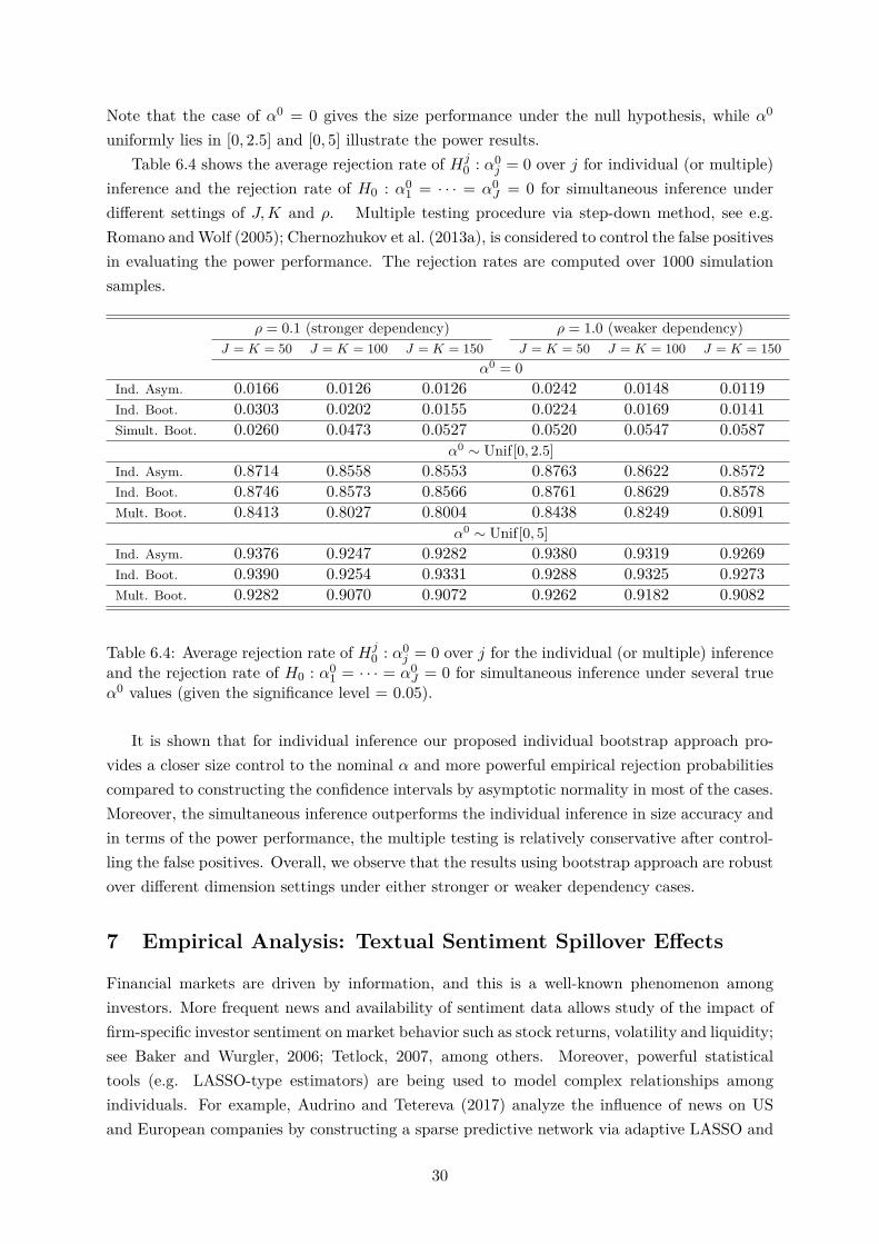
Note that the case of α0 = 0 gives the size performance under the null hypothesis, while α0
uniformly lies in [0, 2.5] and [0, 5] illustrate the power results.Table 6.4 shows the average rejection rate of Hj
0 : α0j = 0 over j for individual (or multiple)
inference and the rejection rate of H0 : α01 = · · · = α0
J = 0 for simultaneous inference underdifferent settings of J,K and ρ. Multiple testing procedure via step-down method, see e.g.Romano andWolf (2005); Chernozhukov et al. (2013a), is considered to control the false positivesin evaluating the power performance. The rejection rates are computed over 1000 simulationsamples.
ρ = 0.1 (stronger dependency) ρ = 1.0 (weaker dependency)J = K = 50 J = K = 100 J = K = 150 J = K = 50 J = K = 100 J = K = 150
j = 0 over j for the individual (or multiple) inferenceand the rejection rate of H0 : α0
1 = · · · = α0J = 0 for simultaneous inference under several true
α0 values (given the significance level = 0.05).
It is shown that for individual inference our proposed individual bootstrap approach pro-vides a closer size control to the nominal α and more powerful empirical rejection probabilitiescompared to constructing the confidence intervals by asymptotic normality in most of the cases.Moreover, the simultaneous inference outperforms the individual inference in size accuracy andin terms of the power performance, the multiple testing is relatively conservative after control-ling the false positives. Overall, we observe that the results using bootstrap approach are robustover different dimension settings under either stronger or weaker dependency cases.
Financial markets are driven by information, and this is a well-known phenomenon amonginvestors. More frequent news and availability of sentiment data allows study of the impact offirm-specific investor sentiment on market behavior such as stock returns, volatility and liquidity;see Baker and Wurgler, 2006; Tetlock, 2007, among others. Moreover, powerful statisticaltools (e.g. LASSO-type estimators) are being used to model complex relationships amongindividuals. For example, Audrino and Tetereva (2017) analyze the influence of news on USand European companies by constructing a sparse predictive network via adaptive LASSO and
30
related testing procedures. In this section the developed technology is applied to study textualsentiment spillover effects across individual stocks. This is different from the "equation-by-equation" analysis in Audrino and Tetereva (2017), since we build up a system of regressionequations and implement the estimation and the inference of the network jointly.
7.1 Data Source
The empirical study in this paper is carried out based on the financial news articles publishedon the NASDAQ community platform from January 2, 2015 to December 29, 2015 (252 tradingdays). The data were gathered via a self-written web scraper to automate the downloadingprocess. The dataset is available at the Research Data Centre (RDC), Humboldt-Universität zuBerlin. Moreover, unsupervised learning approaches are employed to extract sentiment variablesfrom the articles. Two sentiment dictionaries: the BL option lexicon (Hu and Liu, 2004) and theLM financial sentiment dictionary (Loughran and McDonald, 2011) were used in Zhang et al.(2016). For each article i (published on day t), the average proportion of positive/negativewords using BL or LM lexica - PosBL
j,i,t, NegBLj,i,t, PosLM
j,i,t, NegLMj,i,t - are considered as the text
sentiment variables. Furthermore, the bullishness indicator for stock j on day t with the relatedarticles i = 1, . . . ,m (based on a particular lexicon) is constructed by following Antweiler andFrank (2004)
Bj,t = log[1 +m−1m∑i=1
1(Posj,i,t > Negj,i,t)/1 +m−1m∑i=1
1(Posj,i,t < Negj,i,t)]. (7.1)
We refer to Zhang et al. (2016) for more details about the data gathering and processing pro-cedure. 63 individual stocks which are S&P 500 component stocks from 9 Global IndustrialClassification Standard (GICS) sectors are considered. They are traded at NSDAQ Stock Ex-change or NYSE. The list of the stock symbols and the corresponding company names can befound in Table D.1 in Appendix D in the supplementary materials.
The daily log returns Rj,t and log volatilities log(σ2j,t) for the stocks over the same time
span are taken as response variables. More precisely, the Garman and Klass (1980) range-basedmeasure to represent the volatility level is employed:
where uj,t = log(PHj,t) − log(POj,t), dj,t = log(PLj,t) − log(POj,t), rj,t = log(PCj,t) − log(POj,t), withPHj,t, P
Lj,t,, POj,t, and PCj,t denote the highest, lowest, opening and closing prices, respectively.
In addition, the S&P 500 index returns and Chicago Board Options Exchange volatility index(VIX) are included as the state variables. The financial time series data were originally obtainedfrom Datastream, and GICS sector information was found at Compustat.
31
7.2 Model Setting and Results
We now construct a network model to detect the spillover effects from sentiment variables tofinancial variables by
rj,t = cj +B>t βj + z>t γj + rj,t−1δj + εj,t,
log σ2j,t = cj +B>t βj + z>t γj + log σ2
j,t−1δj + εj,t, (7.3)
where j = 1, . . . , J indicate the stock symbols, Bt = (B1,t, . . . , BJ,t)> and zt includes the statevariables.
It is of interest to make inferences on the parameters βj ∈ IRJ , j = 1, . . . J . Followingthe framework introduced in Section 4, an estimation procedure with three steps needs to beimplemented.
S1 For each j, run LASSO on (7.3) and keep the estimator β[1]j(−j), γ
[1]j , δ[1]
j and c[1]j .
S2 For each j, run LASSO on Bj,t = (B>−j,t, z>t , rj,t−1)>θj + vj,t to model the dependenceamong sentiment variables. In particular, we propose to take the joint penalty level ob-tained via block multiplier bootstrap (discussed in Section 3.2) for this regression system.Keep the residuals as vj,t = Bj,t − (B>−j,t, z>t , rj,t−1)>θj .
S3 For each (j, k), run IV regression of rj,t − c[1]j − B>−j,tβ
[1]j(−j) − z
>t γ
[1]j − rj,t−1δ
[1]j on Bk,t
using vk,t as an instrument variable. Then we obtain the final estimator β[2]jk .
If for stock j, the sentiment variable of firm k is selected into the active set after the individualsignificance test i.e., the null hypothesis Hjk
0 : βjk = 0 is rejected under the block multiplierbootstrap procedure (as discussed in Section 6.1 we pre-determine bn = 5 by choosing the onegives the lowest prediction norm in the LASSO estimation in S1 on a grid search), then we puta directional edge from k to j. As a result, we achieve a 0 − 1 adjacency matrix describingthe dependency network from sentiment variable to financial variable. Note that the diagonalelements in the matrix show the self-effect of stocks.
The graphical network for stock returns and volatility modelled by (7.3) based on BL andLM lexica (from 01/02/15 to 12/29/15) is depicted in Figures 7.1-7.2.
32
AA
AAPLACN
ADP
AET
AIG
AMGN
AMT
AMZN
APC
AXP
BA
BAC
BBY
BHI
BIIB
BMY
CCAT
CBS
CELG
CHK
CMCSA
CMG
COP
COST
CSCO
CVS
CVX
DAL
DD
DHR
DIS
DOW
DUK
EA
EBAYEMC
ETFC
EXC
F
FDX
FSLR
GDGE GILD
GM
GPS
GS
HAL
HD
HON
HPQ
IBM
INTC
JNJ
JPM
KO
KR
LEN
LLY
LMT
LUV
return−BL 02/01/15−30/12/15Consumer Discret.
Consumer Staples
Energy
Financials
Health Care
Industrials
Info Tech
Materials
Utilities
AA
AAPLACN
ADP
AET
AIG
AMGN
AMT
AMZN
APC
AXP
BA
BAC
BBY
BHI
BIIB
BMY
CCAT
CBS
CELG
CHK
CMCSA
CMG
COP
COST
CSCO
CVS
CVX
DAL
DD
DHR
DIS
DOW
DUK
EA
EBAYEMC
ETFC
EXC
F
FDX
FSLR
GDGE GILD
GM
GPS
GS
HAL
HD
HON
HPQ
IBM
INTC
JNJ
JPM
KO
KR
LEN
LLY
LMT
LUV
return−LM 02/01/15−30/12/15Consumer Discret.
Consumer Staples
Energy
Financials
Health Care
Industrials
Info Tech
Materials
Utilities
Figure 7.1: The dependency network among individual stocks from sentiment variables to re-turn.
33
AA
AAPLACN
ADP
AET
AIG
AMGN
AMT
AMZN
APC
AXP
BA
BAC
BBY
BHI
BIIB
BMY
CCAT
CBS
CELG
CHK
CMCSA
CMG
COP
COST
CSCO
CVS
CVX
DAL
DD
DHR
DIS
DOW
DUK
EA
EBAYEMC
ETFC
EXC
F
FDX
FSLR
GDGE GILD
GM
GPS
GS
HAL
HD
HON
HPQ
IBM
INTC
JNJ
JPM
KO
KR
LEN
LLY
LMT
LUV
volatility−BL 02/01/15−30/12/15Consumer Discret.
Consumer Staples
Energy
Financials
Health Care
Industrials
Info Tech
Materials
Utilities
AA
AAPLACN
ADP
AET
AIG
AMGN
AMT
AMZN
APC
AXP
BA
BAC
BBY
BHI
BIIB
BMY
CCAT
CBS
CELG
CHK
CMCSA
CMG
COP
COST
CSCO
CVS
CVX
DAL
DD
DHR
DIS
DOW
DUK
EA
EBAYEMC
ETFC
EXC
F
FDX
FSLR
GDGE GILD
GM
GPS
GS
HAL
HD
HON
HPQ
IBM
INTC
JNJ
JPM
KO
KR
LEN
LLY
LMT
LUV
volatility−LM 02/01/15−30/12/15Consumer Discret.
Consumer Staples
Energy
Financials
Health Care
Industrials
Info Tech
Materials
Utilities
Figure 7.2: The dependency network among individual stocks from sentiment variables tovolatility.
Figures 7.1-7.2 depict the dependency networks among individual stocks. Given that thetime series of returns and volatility are scaled and centered before implementing the estimationprocedure, we find even denser spillover effects in the volatility analysis. This indicates thestock volatility is more sensitive to sentiment than returns. Moreover, the relationships betweensectors are also of interest. The simultaneous confidence region constructed via the bootstrapapproach introduced in Section 4.2 may help us to detect whether the sentiment information
34
from one sector has joint influence on the returns of the stocks in another sector. In particular,we look at the null hypothesis: HS1,S2
0 : βjk = 0, ∀j ∈ S1, k ∈ S2, where S1 and S2 representtwo groups of stocks that belong to two sectors, respectively. The conclusion that the sentimentfrom sector S2 has a joint effect on the returns or volatility of sector S1 can be drawn if thenull hypothesis is rejected with the simultaneous confidence region (4.8) under the significancelevel = 0.05.
Consumer Discretionary
Consumer Staples
EnergyFinancials
Health Care
Industrials
Information TechnologyMaterials
Utilities
return−BL sector analysis 02/01/15−30/12/15
Consumer Discretionary
Consumer Staples
EnergyFinancials
Health Care
Industrials
Information TechnologyMaterials
Utilities
return−LM sector analysis 02/01/15−30/12/15
Consumer Discretionary
Consumer Staples
EnergyFinancials
Health Care
Industrials
Information TechnologyMaterials
Utilities
volatility−BL sector analysis 02/01/15−30/12/15
Consumer Discretionary
Consumer Staples
EnergyFinancials
Health Care
Industrials
Information TechnologyMaterials
Utilities
volatility−LM sector analysis 02/01/15−30/12/15
Figure 7.3: The dependency network among sectors from sentiment variables to financial vari-ables.
Figure 7.3 describes the spillover effect network from sentiment to financial variables on thesector levels. In particular, the connections from energy to health care is found to be signifi-cant in the analysis of stock returns; while if volatility is focused on then the spillover effectsfrom financials to health care, from information technology to energy, also from consummerdiscretionary to utilities are detected.
Comment 7.1 (Link to GGM). Another popular way to conduct the network analysis in theliterature is the GGM, which is corresponding to the estimation of a high dimensional precisionmatrix. And under the Gaussian assumption our SRE can be linked to a nodal wise GGM. Inparticular, one can estimate the coefficients in each equation of SRE by using a sparse Graphicalmodel estimation, for example the LASSO type estimation as in Yuan and Lin (2007), and thuswe build the link equation-by- equation.
35
Consider the VAR(1) as an example, the jth equation in the SRE is given by Yj,t = Φj·Yt−1+εj,t, where Yt is covariance stationary with Var(Yt) = Γ (p.d.). Correspondingly, we look at thevector Yj,t = (Yj,t, Y1,t−1, . . . , YJ,t−1)> belonging to an undirected graph (Vj , Ej) with vertex set
It can be seen that Φjk = 0 would imply that the (1, k + 1)th element of Θj is zero and viceversa. In addition, a LASSO type estimator proposed in Yuan and Lin (2007) can be obtainedby solving
Θj = arg maxΘ− log det(Θ) + trace(SjΘ) + λj
∑`k
|Θ`k|,
where Sjdef= n−1∑n
t=1 Yj,tY>j,t.
In an unreported simulation study we compare the estimation performance between ourproposed approach and the nodal wise GGM under the VAR(1) model. The results show thatthe nodal wise GGM which is approximated to SRE has worse prediction performance than ourmethod, which can be obtained from the authors upon request.
36
Supplementary Material
A Theorems for Joint Penalty over Equations
Recall that the theoretical choice λ0(1− α) is defined as the (1− α) quantile ofmax
16k6K,16j6J2c√n|Sjk/Ψjk|. First, we provide the analogue results of Theorem 5.1 and Corollary
5.1.
Theorem A.1. Under (A1) and (A3), we have
P(2c√n max
16k6K,16j6J|Sjk/Ψjk| > r) 6C1$nnr
−qJ∑j=1
K∑k=1
‖Xjk,·εj,·‖qq,ςΨqjk
+ C2
J∑j=1
K∑k=1
exp( −C3r
2Ψ2jk
n‖Xjk,·εj,·‖22,ς
), (A.1)
where for ς > 1/2− 1/q (weak dependence case), $n = 1; for ς < 1/2− 1/q (strong dependencecase), $n = nq/2−1−ςq. C1, C2, C3 are constants depending on q and ς.
Corollary A.1 (Bound for λ0(1−α) and Oracle Inequalities under IC). Under (A1) and (A3),given λ0(1− α) satisfies
λ0(1− α) . max16k6K,16j6J
‖Xjk,·εj,·‖2,ς
√n log(KJ/α) ∨ ‖Xjk,·εj,·‖q,ς(n$nKJ/α)1/q
, (A.2)
additionally assume that the RE condition (A2) holds uniformly over equations j = 1, . . . , Jwith probability 1− O(1), and under the exact sparsity assumption (3.1), then βj obtained from(3.2) under IC satisfy
|βj−β0j |j,pr . C
√s max
16k6KΨjk max
16j6J
‖Xjk,·εj,·‖2,ς
√log(KJ/α)√
n∨‖Xjk,·εj,·‖q,ςn1/q−1($nKJ/α)1/q
,
(A.3)with probability 1 − α − O(1), where for ς > 1/2 − 1/q (weak dependence case), $n = 1; forς < 1/2 − 1/q (strong dependence case), $n = nq/2−1−ςq, and the constant C depends on theRE constants.
The other empirical choices of the joint penalty level can be:
a) Q(1 − α): the (1 − α) quantile of 2c max16k6K,16j6J
√n|Zjk/Ψjk|. In practice, one can take
an alternative choice such that Q(1− α) def= 2c√nΦ−11− α/(2KJ).
b) Λ(1− α) def= 2c√nq
[B](1−α), where q
[B](1−α) is the (1− α) quantile of max
16k6K,16j6J|Z [B]jk /Ψjk|.
For a) again we need the Gaussian approximation results for the vectorized process S def=vec[(Sjk)Kk=1Jj=1] = 1√
n
∑nt=1 Xt, where Xt
def= vec[(Xjk,tεj,t)Kk=1Jj=1] similar to Theorem 5.2and Corollary 5.2 to justify the choice of λ as Q(1− α).
37
Let Xtdef= vec[(Xjk,t)Kk=1Jj=1]. We first aggregate the dependence adjusted norm over
j = 1, . . . , J and k = 1, . . . ,K:
‖|X·|∞‖q,ςdef= sup
m>0(m+ 1)ς
∞∑t=m
δq,t, δq,tdef= ‖|Xt −X ∗t |∞‖q, (A.4)
where q > 1, and ς > 0. Moreover, define the following quantities
Theorem A.2. Under (A1), (A3) and (A4’), for each k = 1, . . . ,K, j = 1, . . . , J assume thatthere exists a constant c > 0 such that min
16k6K,16j6Javar(Sjk) > c, then we have
ρ(D−1S, D−1Z
)→ 0, as n→∞, (A.6)
where Z ∼ N(0,ΣX ), ΣX is the JK × JK long-run variance-covariance matrix of Xt, and D isa diagonal matrix with the square root of the diagonal elements of ΣX , namely
∞∑`=−∞
E(Xjk,tXjk,(t−`)εj,tεj,(t−`))1/2
=√
avar(Sjk), for k = 1, . . . ,K, j = 1, . . . , J.
Corollary A.2. Under the conditions of Theorem A.2, we have
supα∈(0,1)
|P max16k6K,16j6J
2c√n|Sjk/Ψjk| > Q(1− α) − α| → 0, as n→∞. (A.7)
Corollary A.3. Under the conditions of Theorem A.2, and assume Φ2q,ς <∞ with q > 4, bn =O(nη) for some 0 < η < 1. Let Fς = n, for ς > 1− 2/q; Fς = lnb
q/2−ςq/2n , for 1/2− 2/q < ς <
1− 2/q; Fς = lq/4−ςq/2n b
q/2−ςq/2n , for ς < 1/2− 2/q. Given n−1log(KJ)2 max
n1/2b
1/2n Φ2
2q,ς ,
n1/2b1/2n
√log(KJ)Φ2
8,ς , F2/qς Γ2
2q,ς(KJ)2/q,Φ2,0Φ2,ςv′(bn)n/
√log(KJ)
= O(1), where v′(bn) =
(bn + 1)−ς + 2vn,2/bn, vn,2 = log bn (resp. b−ς+1n or 1) for ς = 1 (resp. ς < 1 or ς > 1), then we
haveρ(D−1S, D−1Z
)→ 0, as n→∞, (A.8)
where D = diag(ΣX )1/2, ΣX = 1bnln
∑lni=1
(∑ibnl=(i−1)bn+1 Xl
)(∑ibnl=(i−1)bn+1 Xl
)>.38
Similar to Corollary 5.4, we can provide a refined bound for λ0(1 − α) and also the oracleinequalities under IC as follows.
Corollary A.4 (Bounds for λ0(1−α) and Oracle Inequalities under IC with Gaussian Approxi-mation Results). Under the conditions of Theorem A.2, suppose 2log(KJ)−1/2+ρ(D−1S, D−1Z) =O(α) and let Zα > 2c
√n log(KJ), where c is no less than the c in the definition of λ0(1 − α),
then we have λ0(1− α) satisfyingλ0(1− α) 6 Zα, (A.9)
additionally assume that the RE condition (A2) holds uniformly over equations j = 1, . . . , Jwith probability 1− O(1), and given the exact sparsity assumption (3.1), then βj obtained from(3.2) under IC satisfies
|βj − β0j |j,pr . C
√s max
16k6KΨjk
√log(KJ)√
n, (A.10)
with probability 1− α− O(1), where the constant C depends on the RE constants.
Next, we need to show the validity of b). Let Z [B] def= vec[(Z [B]jk )Kk=1Jj=1] and Ψ def=
vec[(Ψjk)Kk=1Jj=1]. Similarly to Theorem 5.3 we have the following results:
Theorem A.3. Under (A1), (A3), and assume Φ2q,ς < ∞ with q > 4, bn = O(nη) for some0 < η < 1 (the detailed rate is calculated in (B.3)), then
Lastly, we show the performance bounds for the OLS post-LASSO estimator in the followingtheorem.
For each p 6 n, Tj ⊂ 1, · · · ,K, |Tj\Tj | 6 p, we define the class of functionsGTj
= εj,tX>j,tδ/|δ|j,pr, supp(δ) ⊆ Tj , |δ|2 = 1. The covering number of the function class isgiven by supQN (ε,G
Tj, ‖ · ‖Q,1). Also define Fj,p = G
Tj: Tj ⊂ 1, · · · ,K, |Tj\Tj | 6 p. For
any f ∈ Fj,p, there exists a set Fj,p such that minf ′∈Fj,p ‖f − f ′‖Q,1 6 ε, and the cardinality ofthe set is denoted by |Fj,p|. Consider the vector ϑt of length |Fj,p|, such that for l = 1, . . . , |Fj,p|,there is ϑl,t = (f − E f)/ψf with ψf = avar(Gn(f))1/2, corresponding to each f ∈ Fj,p. Theaggregated dependence adjusted norm is given by
‖ϑ·‖q,ςdef= sup
m>0(m+ 1)ς
∞∑t=m‖|ϑt − ϑ∗t |∞‖q, (A.13)
where q > 1, and ς > 0. Moreover, define the following quantities (for simplicity we drop the
39
subscripts j, p)
Φϑq,ς
def= max16l6|Fj,p|
‖ϑl,·‖q,ς , Γϑq,ςdef=( |Fj,p|∑
l=1‖ϑl,·‖qq,ς
)1/q,
Θϑq,ς
def= Γϑq,ς ∧‖ϑ·‖q,ς(log |Fj,p|)3/2. (A.14)
To evoke the Gaussian approximation on Gn(f)/ψf , we need to impose the following assump-tions additionally. Define Lϑ1 = Φϑ
2,ςΦϑ2,0(log |Fj,p|)21/ς ,W ϑ
1 = (Φϑ3,0)6+(Φϑ
4,0)4log(|Fj,p|n)7,W ϑ
2 = (Φϑ2,ς)2log(|Fj,p|n)4, W ϑ
3 = [n−ςlog(|Fj,p|n)3/2Θϑq,ς ]1/(1/2−ς−1/q),
Nϑ1 = (n/ log |Fj,p|)q/2(Θϑ
q,ς)q, Nϑ2 = n(log |Fj,p|)−2(Φϑ
2,ς)−2, Nϑ3 = n1/2(log |Fj,p|)−1/2(Θϑ
q,ς)1/(1/2−ς).
(A7) i) (weak dependency case) Given Θϑq,ς <∞ with q > 2 and ς > 1/2− 1/q, then
Θϑq,ςn
1/q−1/2log(|Fj,p|n)3/2 → 0 and L1 max(W ϑ1 ,W
ϑ2 ) = O(1) min(Nϑ
1 , Nϑ2 ).
ii) (strong dependency case) Given 0 < ς < 1/2− 1/q, then Θϑq,ς(log |Fj,p|)1/2 = O(nς) and
L1 max(W ϑ1 ,W
ϑ2 ,W
ϑ3 ) = O(1) min(Nϑ
2 , Nϑ3 ).
Comment A.1. For a random vector zt ∈ RK , suppose there exist constants C,D > 0, suchthat maxk Eexp(|zk,t/D|q) 6 C. Then by Jensen’s inequality it follows that ‖|zt|∞‖q 6
D(logK + logC)1/q. In particular, for the case of sub-Gaussian random variables, there existsconstant D > 0 such that Eexp(|zk,t/D|2) − 1 6 1, which implies ‖|zt|∞‖2 . D
√logK.
Similar to the discussion in Remark 5.6, consider the case with Θϑq,ς = O((log |Fj,p|)1/q)
and Φϑq,ς = O(1), where ς > 1/2 − 1/q. Then Θϑ
q,ςn1/q−1/2log(|Fj,p|n)3/2 → 0 becomes
log |Fj,p|log(n|Fj,p|)3q/2 = O(nq/2−1), which implies that Lϑ1 max(W ϑ1 ,W
ϑ2 ) = O(1) min(Nϑ
1 , Nϑ2 ).
As shown in the proof of Theorem A.4, |Fj,p| . Kp(6µj(p)σ/ε)s+p withε =
√p logK + (p+ s) log(6µj(p)σ)(4
√n)−1. This means with (A7), the dimension K has to
satisfy the condition p logK + (s+ p) log(√n)1+3q/2 = O(nq/2−1), where we consider the case
such that |Fj,p| is larger than n.
Theorem A.4 (Prediction Performance Bounds for OLS Post-LASSO). Given (A1), (A3) and(A7), suppose (A2) (with c = c+1
c−1 , c > 1) and (A5) (with pj = |Tj \ Tj |) hold uniformly overequations with probability 1 − O(1), then under the exact sparsity assumption (3.1), for anyτ > 0, there is a constant Cτ independent of n, for all j = 1, . . . , J we have
|β[P ]j − β
0j |j,pr 6 Cτ max
16k6KΨjk
√p logK + (p+ s)log(6µj(p)σ) + logn/2
n
+ 1(Tj * Tj)C√s max
16k6KΨjk max
16j6J
‖Xjk,·εj,·‖2,ς
√log(KJ/α)√
n∨ ‖Xjk,·εj,·‖q,ςn1/q−1($nKJ/α)1/q,
(A.15)
with probability 1− α− τ − O(1), where for ς > 1/2− 1/q (weak dependence case), $n = 1; forς < 1/2− 1/q (strong dependence case), $n = nq/2−1−ςq. σ = maxjavar(n−1/2∑n
t=1 εj,t)1/2
and the constant C depends on the RE constants.
In particular, suppose the Gaussian approximation results hold for λ0(1−α), the bound forit can be replaced according to Corollary A.4.
40
B Detailed Proofs
B.1 Proofs of Single Equation Estimation
Proof of Theorem 5.1. For each j = 1, . . . J , k = 1, . . . ,K, applying Theorem 2 of Wu andWu (2016) gives
P(√n|Sjk| > x) 6
C ′1$nn‖Xjk,·εj,·‖qq,ςxq
+ C ′2 exp( −C3x
2
n‖Xjk,·εj,·‖22,ς
),
where for ς > 1/2 − 1/q, $n = 1; for ς < 1/2 − 1/q, $n = nq/2−1−ςq. C ′1, C′2, C3 are three
constants depending on q and ς. It follows that the conclusion holds if we set x = (2c)−1Ψjkr.
Proof of Theorem 5.2. According to the Minkowski’s inequality and Hölder’s inequality, wehave
Consequently, we have the following relationships:
max16k6K
‖Xjk,·εj,·‖q,ς 6 2 max16k6K
‖Xjk,·‖2q,ς‖εj,·‖2q,ς ,
(K∑k=1‖Xjk,·εj,·‖qq,ς)1/q 6 2‖εj,·‖2q,ς(
K∑k=1‖Xjk,·‖q2q,ς)1/q,
‖Xj,·εj,·‖q,ς 6 2‖Xj,·‖2q,ς‖εj,·‖2q,ς .
Therefore, the conditions in Theorem 3.2 of Zhang and Wu (2017a) can be verified for theK-dimensional stationary process Xj,tεj,t. Finally, applying that theorem yields the Gaussianapproximation results.Proof of Corollary 5.2. It follows directly from the Gaussian approximation results in The-orem 5.2.Proof of Corollary 5.3. The proof follows that of Corollary 5.4 in Zhang and Wu (2017a).For w > 0, we have
ρ(D−1j Sj·, D
−1j Zj) = sup
r>0
∣∣P(|D−1j Sj·|∞ > r)− P(|D−1
j Zj |∞ > r)∣∣
6 ρ(D−1j Sj·, D
−1j Zj) + sup
r>0P(||D−1
j Zj |∞ − r| 6 w) + P(|(D−1j − D
−1j )Sj·|∞ > w)
. ρ(D−1j Sj·, D
−1j Zj) + w
√logK + P(|(D−1
j − D−1j )Sj·|∞ > w),
41
where the last line uses the arguments of Theorem 3 in Chernozhukov et al. (2015). Let Vn,jdef=
max16k6K
|Ψjk/Ψjk − 1| and Ln,jdef= max
16k6K|Ψ2
jk − Ψ2jk|. Then |(D
−1j − D
−1j )Sj·|∞ 6 Vn,j |D−1
j Sj·|∞.
As min16k6K
Ψ2jk > cj , let w = xy, 0 < x < cj/2, y > 0, then
P(|(D−1j − D
−1j )Sj·|∞ > w) 6 P(Vn,j > 2x/cj) + P(|D−1
j Sj·|∞ > cjy/2)
6 P(Ln,j > x) + ρ(D−1j Sj·, D
−1j Zj) + P(|D−1
j Zj |∞ > cjy/2).
It follows that
ρ(D−1j Sj·, D
−1j Zj) 6 ρ(D−1
j Sj·, D−1j Zj) + xy
√logK + P(Ln,j > x) + P(|D−1
j Zj |∞ > cjy/2).
In particular, Ln,j 6 Ln,j,1 + Ln,j,2, with Ln,j,1 = max16k6K |Ψ2jk − E Ψ2
jk| and Ln,j,2 =max16k6K |E Ψ2
jk − Ψ2jk|.
As for Ln,j,1, applying Theorem 5.1 of Zhang and Wu (2017a), for u > n1/2b1/2n Φ2
j,2q,ς , wehave
P(nLn,j,1 > u) .FςΓqj,2q,ςuq/2
+K exp(− Cju
2
nbnΦ4j,8,ς
),
where the constants Cj depend on η, q, and ς. Then we have P(Ln,j,1 > x)→ 0, as n→∞, ifwe set x =
√logKn max
n1/2b
1/2n Φ2
j,2q,ς , n1/2b
1/2n√
logKΦ2j,8,ς , F
2/qς Γ2
j,2q,ς.
For Ln,j,2, define v′(bn) = (bn + 1)−ς + 2vn,2/bn, vn,2 = log bn (resp. b−ς+1n or 1) for ς = 1
(resp. ς < 1 or ς > 1). It can be shown that Ln,j,2 6 Φj,2,0Φj,2,ςv′(bn). Note that v′(bn) is
a special case of v(bn) in the proof of Theorem 5.3 given n → ∞, and the conclusion followssimilarly.
It follows that P(Ln,j > x)→ 0, as n→∞, if we set
x =√
logKn
maxn1/2b1/2n Φ2
j,2q,ς , n1/2b1/2n
√logKΦ2
j,8,ς , F2/qς Γ2
j,2q,ς ,Φj,2,0Φj,2,ςv′(bn)n/
√logK
.
Moreover, given Theorem 5.2 and choosing y = C√
logK (the constant C > 0 is sufficientlylarge) yields the conclusion.Proof of Corollary 5.4. Let ρn
def= ρ(D−1j Sj·, D
−1j Zj) and by its definition, we have
P(2c√n max
16k6K|Sjk/Ψjk| 6 Zα) > P(2c
√n max
16k6K|Zjk/Ψjk|| 6 Zα)− ρn
> 1−K∑k=1
P|Zjk/Ψjk| > Zα/(2c√n) − ρn
> 1−K∑k=1
2Zα/(2c√n)−1 exp[−Z2
α/2(2c√n)2]− ρn
> 1− 2(logK)−1/2 − ρn,
where we have applied the union bound, the tail probability of Gaussian random variable and thefact that Zα = 2c
√n logK > 2c
√n logK (c is no less than the c in the definition of λ0
j (1−α)).It follows that λ0
j (1 − α) 6 Zα as 1 − α = P2c√n max
16k6K|Sjk/Ψjk| 6 λ0
j (1 − α) 6
42
P(2c√n max
16k6K|Sjk/Ψjk| 6 Zα), given 2(logK)−1/2 + ρn = O(α) (note that Theorem 5.2 en-
sures that ρn → 0 with a polynomial rate as n→∞).
Proof of Theorem 5.3. Let Sjk,i = 1√n
∑ibnl=(i−1)bn+1Xjk,lεj,l, we first need to prove that
ρn,jdef= sup
r∈IR
∣∣P max16k6K
(Z [B]jk /Ψjk) 6 r|Xj,·, εj,·
− P
max
16k6K(Zjk/Ψjk) 6 r
∣∣= sup
r∈IR
∣∣P max16k6K
( ln∑i=1
ej,iSjk,i/Ψjk
)6 r|Xj,·, εj,·
− P
max
16k6K(Zjk/Ψjk) 6 r
∣∣→ 0, as n→∞.
Given the sample variance covariance matrix (K × K) Σj,n =∑n`=−n(1 − |`|/n)Γj(`), where
Γj(`) = E(Xj,tεj,tX>j,t−`εj,t−`), let Zj = (Zjk)Kk=1 ∼ N(0,Σj,n). In addition, define Σj,bn =∑bn
`=−bn(1 − |`|/bn)Γj(`) and Σj =∑lni=1 Sj,iS
>j,i, where Sj,i = (Sjk,i)Kk=1. Let Ψj = diag(Ψjk),
δj = δj1+δj2, with δj1 = |Ψ−1j ΣjΨ−1
j −Ψ−1j Σj,bnΨ−1
j |max and δj2 = |Ψ−1j Σj,bnΨ−1
j −Ψ−1j Σj,nΨ−1
j |max,where | · |max is the maximum norm of a matrix. According to Theorem 2 of Chernozhukov et al.(2015), ρn,j is bounded by π(δj1)∨π(δj2), with π(δj)
def= Cδ1/3j 1∨a2
K ∨ log(1/δj)1/3(logK)1/3,where aK = E( max
16k6KZjk/Ψjk) 6
√2 logK.
For the first part,
δj1 = max16k1,k26K
∣∣∣∣∑lni=1 Sjk1,iSjk2,i
Ψjk1Ψjk2
− ln E(Sjk1,iSjk2,i)Ψjk1Ψjk2
∣∣∣∣6
max16k1,k26K
∣∣∑lni=1 Sjk1,iSjk2,i − ln E(Sjk1,iSjk2,i)
∣∣min
16k1,k26KΨjk1Ψjk2
.
We need to analyze the tail probability of δj1. Applying Theorem 5.1 of Zhang and Wu (2017a),for x > n1/2b
1/2n Φ2
j,2q,ς , we have
P(nδj1 >
x
min16k1,k26K
Ψj1k1Ψj2k2
).KFςΓqj,2q,ς
xq/2+K2 exp
(− Cjx
2
nbnΦ4j,8,ς
),
for all large n, where Fς = n, for ς > 1 − 2/q; Fς = lnbq/2−ςq/2n , for 1/2 − 2/q < ς < 1 − 2/q;
Fς = lq/4−ςq/2n b
q/2−ςq/2n , for ς < 1/2−2/q. The constants Cj depend on η, q, and ς. This ensures
that when x = maxn1/2b
1/2n Φ2
j,2q,ς , n1/2b
1/2n (logK)1/2Φ2
j,8,ςcn,K2/qF
2/qς Γ2
j,2q,ςcn, c−1
n = O(1),the tail probability tends to 0, as n→∞.
It follows that π(δj1)→ 0 as n→∞, given x = On(logK)−2, which implies the followingconditions on bn:
bn = On(logK)−4Φ−4j,2q,ς ∧ n(logK)−5Φ−4
j,8,ςc−2n , Fς = Onq/2(logK)−qK−1Γ−qj,2q,ςc
−q/2n .
For the second part, by defining ψjdef= min
16k1,k26KΨjk1Ψjk2 , we have
δj2 6∣∣∣∣ψ−1j
∑bn<|`|6n
(1− |`|/n)Γj(`) +bn∑
`=−bn|`|(−1/n+ 1/bn)Γj(`)
∣∣∣∣max
.
43
Recall that
|Γj,k1,k2(`)| =∣∣∣∣ ∞∑h=0
E(Ph(Xjk,0εj0)Ph(Xjk2,`εj,`)∣∣∣∣
6∞∑h=0‖Xjk1,hεj,h −X∗jk1,hε
∗j,h‖2‖Xjk2,h+`εj,h+` −X∗jk2,h+`ε
∗j,h+`‖2,
where the operator is given by Ph(·) def= E(·|Fh)− E(·|Fh−1). It follows that
∣∣∣∣ ∑bn<|`|6n
(1− |`|/n)Γj,k1,k2(`) +bn∑
`=−bn|`|(−1/n+ 1/bn)Γj,k1,k2(`)
∣∣∣∣6 ∆0,2,j,k1∆bn+1,2,j,k2 + 2
n∆0,2,j,k1
n∑`=bn+1
∆`,2,j,k2 + 2n− bnnbn
∆0,2,j,k1
bn∑`=1
∆`,2,j,k2 , (B.1)
where ∆m,2,j,k =∑∞t=m ‖Xjk,tεj,t −X∗jk,tε∗j,t‖2. Given the fact that ∆0,2,j,k 6 Φj,4,0, ∆`,2,j,k 6
Φj,4,ς`−ς , (B.1) is bounded by Φj,4,0Φj,4,ς(bn + 1)−ς + 2n−1∑n
`=bn+1 `−ς + 2n−bnnbn
∑bn`=1 `
−ς =Φj,4,0Φj,4,ςv(bn) for any k1, k2, where v(bn) is a function with respect to bn. Note that v(bn) .(bn + 1)−ς + 2vn,1/n + 2(n − bn)vn,2/(nbn), where vn,1 = logn/(bn + 1) (resp. n−ς+1 or(bn + 1)−ς+1) for ς = 1 (resp. ς < 1 or ς > 1), vn,2 = log bn (resp. b−ς+1
n or 1) for ς = 1 (resp.ς < 1 or ς > 1). Therefore, the bound of δj2 would decrease as bn increases. In particular, weneed to impose an addition assumption such that Φj,4,0Φj,4,ςv(bn) = O(logK)−2 to guaranteeπ(δj2)→ 0.
The results for the two parts above ensure that ρn,j → 0 as n→∞, given x = On(logK)−2and Φj,4,0Φj,4,ςv(bn) = O(logK)−2, which imply the following conditions on bn:
At last, combining the Gaussian approximation results for Sjk/Ψjk and applying Theorem3.1 in Chernozhukov et al. (2013a), we have
supα∈(0,1)
∣∣P ( max16k6K
|Sjk/Ψjk| > q[B]j,(1−α)
)− α
∣∣ . ρn,j + π′(z) + P(δj > z),
where π′(z) = z1/31 ∨ log(K/z)2/3. We need to pick z such that π′(z) + P(δj > z) → 0 asn→∞ and it can be obtained by taking z = r
1/2n /(logK), with
rn = n−1 maxn1/2b
1/2n Φ2
j,2q,ς , n1/2b
1/2n (logK)1/2Φ2
j,8,ςcn,K2/qF
2/qς Γ2
j,2q,ςcn, nΦj,2,0Φj,2,ςv(bn),
c−1n = O(1).
Comment B.1 (Admissible rate of bn). Consider the special case with Φj,2q,ς = O(1) and
44
Γj,2q,ς = O(1), for q > 4. Let K = O(nr), logK = O(r logn) = O(nr), cn = ns with s > 0 andassume 1/2 − 2/q < ς < 1 − 2/q. Then (B.2) implies an admissible rate of bn = O(nη) suchthat 2r/ς < η < max1− 5r − 2s, (q/2− qr − qs/2− r − 1)/(q/2− ςq/2− 1).
Comment B.2 (Validity of multiplier block bootstrap under stronger tail assumptions). Notethat in case with stronger exponential moment conditions on the underlying processes, we shallchange the tail probabilities to bound δj1.
Let Φj,ψν ,ς = max16k6p
supq>2
q−ν‖Xjk,·εj,·‖q,ς < ∞, then according to Theorem 5.2 of Zhang and
Wu (2017a), for all x > 0, we have
P(nδj1 >x
min16k1,k26K
Ψj1k1Ψj2k2
) . K2 exp(− xγ
4eγ(√nbnΦ2
j,ψν ,0)γ),
where γ = 1/(2ν + 1). This implies that when x = (logK√nbnΦ2
j,ψν ,0)1/γcn, with c−1n = O(1),
the tail probability tends to 0, as n → ∞. It follows that π(δj1) → 0 as n → ∞, givenx = (logK
√nbnΦ2
j,ψν ,0)1/γ = On(logK)−2. As a result, (B.2) will be replaced by
Proof of Theorem A.3. Analogue to the proof of Theorem 5.3, the conclusions are impliedby
P(nδ1 >
(min
16k1,k26K,16j1,j26JΨj1k1Ψj2k2
)−1x
).JKFςΓq2q,ς
xq/2+ (JK)2 exp
(− Cx2
nbnΦ48,ς
),
for x > n1/2b1/2n Φ2
2q,ς and all large n, where
δ1def= max
16k1,k26K,16j1,j26J
∣∣∣∣∑lni=1 Sj1k1,iSj2k2,i
Ψj1k1Ψj2k2
− ln E(Sj1k1,iSj2k2,i)Ψj1k1Ψj2k2
∣∣∣∣.In particular, when x = max
n1/2b
1/2n Φ2
2q,ς , n1/2b
1/2n log(JK)1/2Φ2
8,ςcn, (JK)2/qF2/qς Γ2
2q,ςcn,
c−1n = O(1), the tail probability tends to 0, as n→∞.
By similar proof to that of Theorem 5.3, it follows that ρn → 0 as n → ∞, given x =O[nlog(KJ)−2] and Φ4,0Φ4,ςv(bn) = O(logKJ)−2, which imply the following conditions on
45
bn:
bn = O[nlog(KJ)−4Φ−42q,ς ∧ nlog(KJ)−5Φ−4
8,ς c−2n ],
Fς = O[nq/2log(KJ)−q(KJ)−1Γ−q2q,ςc−q/2n ], with c−1
Recall that Fς = n, for ς > 1 − 2/q; Fς = lnbq/2−ςq/2n , for 1/2 − 2/q < ς < 1 − 2/q; Fς =
lq/4−ςq/2n b
q/2−ςq/2n , for ς < 1/2− 2/q.
The rest of the proof is similar to that of Theorem 5.3 and thus is omitted.
Proof of Theorem A.4. For any δ, δ ∈ IRK in GTj, we have
∣∣∣∣Enεj,t(X>j,tδ|δ|j,pr−X>j,tδ
|δ|j,pr
)∣∣∣∣ =∣∣∣∣En[εj,tX>j,t(δ − δ)|δ|j,pr
+X>j,tδ
|δ|j,pr−X>j,tδ
|δ|j,pr
]∣∣∣∣6∣∣∣∣En[εj,tX>j,t(δ − δ)|δ|j,pr
]∣∣∣∣+ ∣∣∣∣En[εj,tX>j,tδ|δ|j,pr−X>j,tδ
|δ|j,pr
]∣∣∣∣6 (Enε2
j,t)1/2
En∣∣∣∣X>j,t(δ − δ)|δ|j,pr
∣∣∣∣21/2+ (Enε2
j,t)1/2( |δ|j,pr − |δ|j,pr
|δ|j,pr
)6 2σµj(p)|δ − δ|2.
Then by following the proof of Lemma 5 (Step 2) in Belloni and Chernozhukov (2013), we havesupQN (ε,G
Tj, ‖ · ‖Q,1) . (6µj(p)σ/ε)s+p. And it follows that |Fj,p| .
(Kp
)(6µj(p)σ/ε)s+p.
Moreover, it is not hard to see that supf∈Fj,p |Gn(f)| 6 2√nε + supf∈Fj,p |Gn(f)|. Let
ψ = maxf∈Fj,p ψf (assume ψ is bounded by constant) and applying the Gaussian approximationresults on the vector Gn(f)/ψf (given (A6)), we have
P
supf∈Fj,p
|Gn(f)| > κn/26 P
supf∈Fj,p
|Gn(f)/ψf | > κn/(2ψ)
6 2|Fj,p|1− Φ(κn/(2ψ))+ dn
6 2Kp(6µj(p)σ/ε)s+p exp−κ2n/(8ψ2)κn/(2ψ)−1 + dn,
as(Kp
)6 Kp. Therefore, for κn = ψ
√p logK + (p+ s)log(6µj(p)σ) + logn/2 and ε =√
p logK + (p+ s) log(6µj(p)σ)(4√n)−1, it follows that supf∈Fj,p |Gn(f)| 6 κn (note that dn →
0 with a polynomial rate as n→∞).The rest of the proof is a direct application of Theorem 5 of Belloni and Chernozhukov (2013)
by inserting the bound for λ0(1−α) (A.2) provided in Corollary A.1, and thus is omitted.
B.3 Plausibility of RE and RSE Conditions
Define the s-sparse sphere as Fδ = δ : |δ|0 6 s, |δ|2 = 1. According to Rudelson and Zhou(2012), the ε-covering number of Fδ w.r.t. the Euclidean metric is l = exp(s log(3eK/mε)), with
46
m > 1. This is the cardinality of the ε-cover set Πδ of Fδ. Moreover, for any point δ ∈ Fδ, let πδdenote the closest point to δ within Πδ. Let X
π(δ)j,t
def= X>j,tπ(δ)2 − n−1π(δ)> EXj,tX>j,tπ(δ),
where Xjdef= n−1/2Xj and Xj(n × K) is a matrix of Xj,t. Note that Xπ(δ)
j,t is a vector of thecardinality of Πδ.
Theorem B.1 (Plausibility of RE and RSE). For any j = 1, . . . , J , suppose the vectors Xj,t oflength K satisfy
0 < κ 6 min|δ|06s,|δ|1=1
δ> E(Xj,tX>j,t)δ 6 max
|δ|06s,|δ|1=1δ> E(Xj,tX
>j,t)δ 6 ψ <∞,
where ψ and κ are positive constants. Given Φ2,ςdef= max
We first check the right hand side of (B.4). Define ‖Xj‖2,Fδdef= sup
δ∈Fδ|Xjδ|2. As indicated in the
proof of Theorem 16 in Rudelson and Zhou (2012), we have |Xjδ − π(δ)|2 6 ε‖Xj‖2,Fδ . Tobound max
π(δ)∈Πδ|Xjπ(δ)|2, we invoke the tail probability inequality in Lemma B.2, which gives
P(
maxπ(δ)∈Πδ
∣∣ n∑t=1
Xπ(δ)j,t
∣∣ > x)
= P[
maxπ(δ)∈Πδ
∣∣|Xjπ(δ)|22 − π(δ)> EXj,tX>j,tπ(δ)
∣∣ > x]→ 0, as n→∞,
if x &√n log lΦ2,ς + rς(log l)3/2∥∥ max
π(δ)∈Πδ|Xπ(δ)
j,· |∥∥q,ς.
Therefore, given κ, ψ > 0, κ − xn 6 |Xjπ(δ)|22 6 xn + ψ holds with probability 1 − O(1)for all π(δ) ∈ Πδ, where xn
def=√n log lΦ2,ς + rς(log l)3/2∥∥ max
π(δ)∈Πδ|Xπ(δ)
j,· |∥∥q,ς. In particular, the
assumptionn−1/2(log l)1/2Φ2,ς + n−1rς(log l)3/2∥∥ max
π(δ)∈Πδ|Xπ(δ)
j,· |∥∥q,ς
= O(1)
ensures that xn = O(1).Hence, the right inequality in (B.4) leads to |Xjδ|2 6 ε‖Xj‖2,Fδ + √xn +
√ψ. Taking the
supremum over all δ ∈ Fδ on both sides shows that supδ∈Fδ|Xjδ|2 6 (√xn +
√ψ)/(1 − ε) with
probability 1 − O(1). Moreover, by the left hand side of (B.4), we have |Xjδ|2 >√κ− xn −
ε(√xn +√ψ)/(1− ε), with probability 1− O(1).
47
Collecting the results together, we have shown that for all δ ∈ Fδ,
√κ− xn −
ε(√xn +√ψ)
(1− ε) 6 |Xjδ|2 6√xn +
√ψ
(1− ε) , (B.5)
with probability 1− O(1).Let c∗(s) = maxδ∈Fδ |Xjδ|2, c∗(s) = minδ∈Fδ |Xjδ|2, with properly chosen ε, c∗(s), c∗(s) are
bounded from above and below, and the desired results follow by the fact κ2j (p) > c∗(sj + p),
φj(p) 6 c∗(sj + p), with sj + p 6 s.
B.4 Proofs of Simultaneous Inference
B.4.1 Some Useful Lemmas
Lemma B.1 (Burkholder (1988)). Let q > 1, q′ = min(q, 2). Let Mn =∑nt=1 ξt; where ξt ∈ Lq
(i.e., ‖ξt‖q <∞) are martingale differences. Then
‖Mn‖q′q 6 Kq′
q
n∑t=1‖ξt‖q
′q where Kq = max((q − 1)−1,
√q − 1).
Lemma B.2 (Theorem 6.2 of Zhang and Wu (2017a) Tail probabilities for high dimensionalpartial sums). For a zero-mean p-dimensional random variable Xt ∈ IRp, let Sn =
∑nt=1Xt and
assume that ‖|X·|∞‖q,ς <∞, where q > 2 and ς > 0, and Φ2,ς = max16j6p
‖Xj,·‖2,ς <∞.
i) If ς > 1/2− 1/q, then for x &√n log pΦ2,ς + n1/q(log p)3/2‖|X·|∞‖q,ς ,
P(|Sn|∞ > x) 6Cq,ςn(log p)q/2‖|X·|∞‖qq,ς
xq+ Cq,ς exp
(−Cq,ςx2
nΦ22,ς
).
ii) If 0 < ς < 1/2− 1/q, then for x &√n log pΦ2,ς + n1/2−ς(log p)3/2‖|X·|∞‖q,ς ,
P(|Sn|∞ > x) 6Cq,ςn
q/2−ςq(log p)q/2‖|X·|∞‖qq,ςxq
+ Cq,ς exp(−Cq,ςx2
nΦ22,ς
).
Lemma B.3 (Tail probabilities for high dimensional partial sums with strong tail assumptions).For a zero-mean p- dimensional random variable Xt ∈ IRp, let Sn =
∑nt=1Xt and assume that
Φψν ,ς = max16j6p
supq>2
q−ν‖Xj,·‖q,ς <∞ for some ν > 0, and let γ = 2/(1 + 2ν). Then for all x > 0,
we haveP(|Sn|∞ > x) 6 p exp−Cγxγ/(
√nΦψν ,0)γ.
Lemma B.4 (Theorem 1 of El Machkouri et al. (2013)). Denote Yt = f(Ft), where f is somemeasurable function. Let Sn =
∑nt=1 Yt, and δς,t = ‖Yt − Y ∗t ‖ς . If E(Yi) = 0,
∑∞t=0 δς,t < ∞,
some ς > 2, and σ2n
def= E(S2n)→∞, then
σ−1n Sn
L→ N(0, 1).
Lemma B.5. Under the same conditions as in Theorem 5.4, let βjk be any estimator such that
48
|βjk − β0jk| 6 Cρn with probability 1− O(1). Then we have
n−1 max(j,k)∈G
∆n . O(n−1/2g−1n ), (B.6)
holds with probability 1− O(1), where ∆ndef= n1/2Gnψjk(Zj,t, βjk, hjk)− ψjk(Zj,t, β0
jk, h0jk).
Proof of Lemma B.5.As indicated in the proof of Theorem 2 in Belloni et al. (2015b), the entropy ent(ε, F) 6
cs log(an/ε) for the function class F = z 7→ ψjkz, β, h(xj(−k)) − ψjkz, β0jk, h
0jk(xj(−k)) :
(j, k) ∈ G, β ∈ Bjk, |β−β0jk| 6 Cρn, h ∈ Hjk, which has 2F as the envelope (the definition of F
is given in (C6)). Therefore, for any f ∈ F , there exists a set Fn such that minf ′∈Fn ‖f−f ′‖Q,2 6
ε, where ε def= ε‖2F‖Q,2 and the cardinality of the set |Fn| = (an/ε)cs. Then we have
supf∈F
∣∣∣∣ n∑t=1
[f − π(f)− Ef − π(f)
]∣∣∣∣ 6 2εn,
where π(f) def= arg minf ′∈F‖f − f ′‖Q,2. Hence, with probability 1− O(1),
β0jk). To this end, we define the following quantities:
Φhm,2,ς
def= maxh∈F hn
∥∥|Xjk· ∂hmg(Zj,·, β, h)|∞
∥∥2,ς , Ωh
m,q,ςdef=∥∥maxh∈F hn
|Xjk· ∂hmg(Zj,·, β, h)|∞
∥∥q,ς. (B.9)
Let χmtdef= ∂hmg(Zj,t, β, h)hm(Xj(−k),t)−h0
jk,m(Xj(−k),t) and define the projector operatorPl(χmt ) def= E(χmt |Fl)− E(χmt |Fl−1). According to Theorem 1(i) of Wu (2005), it is not hard tosee that ‖χm· ‖q,ς . supd>0(d+1)ς
∑∞t=d ‖P0(χmt )‖q, form = 1, 2. Moreover, as |θjk,m−θ0
jk,m|1 .√sjρn 6
√sρn, we have
‖P0(χmt )‖q 6(
E[P0|∂hmg(Zj,t, β, h)Xjkt |∞|θjk,m − θ0
jk,m|1]q)1/q
.√sρn
(E[P0|∂hmg(Zj,t, β, h)Xjk
t |∞]q)1/q
.
50
It follows that ‖χm· ‖q,ς .√sρn
∥∥|Xjk· |∞|∂hmg(Zj,·, β, h)|
∥∥q,ς. Then applying the tail probability
bounds in Lemma B.2 yields with probability approaching 1,
maxh∈F hn
∣∣ n∑t=1
∂hmg(Zj,t, β, h)hm(Xj(−k),t)− h0jk,m(Xj(−k),t)
∣∣ . rN1,m + rςrN2,m,
where rN1,m =√nsρnlog(an/ε)1/2Φh
m,2,ς , rN2,m = s2ρnlog(an/ε)3/2Ωhm,q,ς , and the rates of
Φhm,2,ς and Ωh
m,q,ς are restricted in (C9).Similarly, by defining
Φβ2,ς
def= maxβ∈Fβn
∥∥∂βg(Zj,·, β, h)∥∥
2,ς , Ωβq,ς
def=∥∥ maxβ∈Fβn
|∂βg(Zj,·, β, h)|∥∥q,ς, (B.10)
we have
maxβ∈Fβn
∣∣ n∑t=1
∂βg(Zj,t, β, h)(β − β0jk)∣∣ . rN1,0 + rςrN2,0,
where rN1,0 = ρn√ns log(an/ε)Φβ
2,ς , rN2,0 = ρns log(an/ε)3/2Ωβq,ς . And (C9) constrains the
rates of Φβ2,ς and Ωβ
q,ς .As a result, with probability 1− O(1),
Nn . ρNn , (B.11)
by letting maxm∈0,1,2
rN1,m + rςrN2,m = O(ρNn).
As P(Kn + Nn > x) 6 P(Kn > x/2) + P(Nn > x/2) and collecting the results from (B.7),(B.8), and (B.11), we have shown that ∆n satisfies
n−1 max(j,k)∈G
∆n . ρ∆n ,
where ρ∆n = n−1(ρKn + ρNn) = O(n−1/2g−1n ) (given ε is sufficiently small, and using (C8) and
(C9)).
Comment B.3. [The rates of Ωhm,q,ς and Ωβ
q,ς ] It is worth discussing the rates of Ωhm,q,ς and
Ωβq,ς by the definition under some special cases. For example, consider the VAR(1) model as in
Comment 5.3 given by Yt = AYt−1 + εt, where Yt, εt ∈ IRJ , and εt ∼ i.i.d.N(0,Σ). At first, asshown in the proof of Theorem 5.2, we have
Ωhm,q,ς =
∥∥maxh∈F hn
|Xjk· ∂hmg(Zj,·, β, h)|∞
∥∥q,ς
.∥∥ max
(j,k)∈G|Xjk· |∞
∥∥2q,ς∥∥maxh∈F hn
∂hmg(Zj,·, β, h)∥∥
2q,ς .
For the first term, it is not hard to see that
∥∥ max(j,k)∈G
|Xjkt |∞ − |(X
jkt )∗|∞
∥∥2q . |A|
t−1∞ ‖|ε0|∞‖2q . J1/(2q),
where the last inequality is by the union bound, assuming |A|∞ < 1, and the qth moments of
51
εj,0 (∀j) are bounded by a constant µq. As for the second term, let dndef= |G| ∨ J . In the mean
regression case, for f ∈ F , E(f(zt)|Ft−1) = Xjk,t(β0jk − β) + h0
1 − h1(vjk,t + h02 − h2), it can
be seen that
∥∥maxh∈F hn
∂h1g(Zj,t, β, h)− ∂h1g(Z∗j,t, β, h)∥∥
2q
6∥∥ max
(j,k)∈G|vjk,t − v∗jk,t|
∥∥2q +
∥∥ max(j,k)∈G
|X>j(−k),t − (X>j(−k),t)
∗| maxγj(−k)
|γ0j(−k) − γj(−k)|
∥∥2q
. d1/(2q)n (1 ∨ s1/2ρn),
while in the median regression case, for f ∈ F , E(f(zt)|Ft−1) = [12 − Fεj,t|Ft−1Xjk,t(β0
jk − β) +h0
1 − h1](vjk,t + h02 − h2),
∥∥maxh∈F hn
∂h1g(Zj,t, β, h)− ∂h1g(Z∗j,t, β, h)∥∥
2q
.∥∥ max
(j,k)∈G|vjk,t − v∗jk,t|
∥∥4q +
∥∥ max(j,k)∈G
|X>j(−k),t − (X>j(−k),t)
∗| maxγj(−k)
|γ0j(−k) − γj(−k)|
∥∥4q
. d1/(4q)n (1 ∨ s1/2ρn),
where we use the assumption such that the 4qth moment of the conditional density is bounded.Moreover, we have
∥∥maxh∈F hn
∂h2g(Zj,t, β, h)− ∂h2g(Z∗j,t, β, h)∥∥
2q
6∥∥ max
(j,k)∈G|(Xj(−k),t −X∗j(−k),t)(β
0jk − β)|
∥∥2q
+∥∥ max
(j,k)∈G
|X>j(−k),t − (X>j(−k),t)
∗| maxβj(−k)
|β0j(−k) − βj(−k)|
∥∥2q
. d1/(2q)n (1 ∨ s1/2ρn),
or∥∥maxh∈F hn ∂h2g(Zj,t, β, h)− ∂h2g(Z∗j,t, β, h)
∥∥2q = O(1) for the two cases. Therefore, we are
able to conclude that Ωhm,q,ς . d
1/qn (1 ∨ s1/2ρn) or Ωh
m,q,ς . d3/(4q)n (1 ∨ s1/2ρn), respectively.
Similarly, it can be shown that Ωβq,ς . d
1/qn s1/2ρn or Ωβ
q,ς . d1/(2q)n s1/2ρn for the two cases,
since
∥∥ maxβ∈Fβn
|∂βg(Zj,·, β, h)|∥∥q
.∥∥ max
(j,k)∈G|X>j(−k),t − (X>j(−k),t)
∗|∥∥
2q∥∥ max
(j,k)∈G|X>j(−k),t − (X>j(−k),t)
∗γ0j(−k) − γj(−k)|
∥∥2q
. d1/qn s1/2ρn,
52
or
∥∥ maxβ∈Fβn
|∂βg(Zj,·, β, h)|∥∥q
.∥∥ max
(j,k)∈G|X>j(−k),t − (X>j(−k),t)
∗|∥∥
4q∥∥ max
(j,k)∈G|X>j(−k),t − (X>j(−k),t)
∗γ0j(−k) − γj(−k)|
∥∥4q
. d1/(2q)n s1/2ρn.
In addition, a similar derivation can show that ‖F (zt)‖q . d1/qn (1 ∨ ρn) and
∥∥ max(j,k)∈G
|ψ0jk,·|
∥∥q,ς
.
d1/qn (1 ∨ ρn).
Lemma B.6. Under the same conditions as in Theorem 5.4, we have with probability 1−O(1),
max(j,k)∈G
|E nψjkZj,t, β0jk, h
0jk(Xj(−k),t)| . rn. (B.12)
Proof of Lemma B.6. Consider the class of function FG = z 7→ ψjkz, β0jk, h
0jk(xj(−k)) :
(j, k) ∈ G, the cardinality of the set is |G|. Therefore, the corresponding covering numberis given by supQN (ε‖FG‖Q,2,FG, ‖ · ‖Q,2) = |G|/ε, with FG = supf∈FG |f |. Let ψ0
jk,tdef=
ψjkZj,t, β0jk, h
0jk(Xj(−k),t) and applying the tail probability bounds in Lemma B.2, we have
with probability 1− O(1),
max(j,k)∈G
|E nψ0jk,t| . n−1(r1 + rςr2) . rn, (B.13)
where r1 = (n log an)1/2 max(j,k)∈G
‖ψ0jk,·‖2,ς , r2 = (log an)3/2‖ max
(j,k)∈G|ψ0jk,·|‖q,ς , rς = n1/q for ς >
1/2− 1/q and rς = n1/2−ς for ς < 1/2− 1/q.
Lemma B.7. Under the same conditions as in Theorem 5.4, consider the class of functionsF ′ = z 7→ ψjkz, β, h(xj(−k)) : (j, k) ∈ G, β ∈ Bjk, h ∈ Hjk ∪ h0
jk, we have with probability1− O(1),
n−1/2 supf∈F ′
|Gn(f)| . ρn. (B.14)
Proof of Lemma B.7. The covering number of the function class F ′ is given bysupQN (ε‖F ′‖Q,2,F ′, ‖ · ‖Q,2) = (an/ε)cs, with F ′ = supf∈F ′ |f |. Also, for any f ∈ F ′, thereexists a set F ′n such that minf ′∈F ′n ‖f − f
′‖Q,2 6 ε‖F ′‖Q,2 and the cardinality of the set |F ′n| =(an/ε)cs.
One can apply the technique we used in the proof of Lemma B.5 to achieve the concentrationinequality. Similarly, consider the function set F ′n, for each f ∈ F ′n, let ϕl,t
def= f(zt) andϕl,t
def= ϕl,t − E(ϕl,t|Ft−1, Xj(−k),t), l = 1, . . . , |F ′n|. We have
n|maxf∈F ′n|E nf−E n E(f |Ft−1, Xj(−k),t)| . 4
√ns log(an/ε) max
f∈F ′‖f(zt)‖2+rςs log(an/ε)3/2‖4F ′(zt)‖q.
For each f ∈ F ′n, there exists a function g such that g(zt, β, h) = Ef(zt)|Ft−1, Xj(−k),t −Ef(zt), where β ∈ Bjk, h ∈ Hjk ∪ h0
jk, (j, k) ∈ G. As by the mean value theorem and the
53
continuity of the function g, we have
g(Zj,t, β, h) =∂βg(Zj,t, β, h)(β − β0jk)
+2∑
m=1∂hmg(Zj,t, β, h)hm(Xj(−k),t)− h0
jk,m(Xj(−k),t),
where (β, h(·)) is the corresponding point which joins the line segment between (β, h(·)) and(β0jk, h
0jk(·)). Let F ′βn and F ′hn collect all the points of β and h according to F ′n, and define the
following quantities (m = 1, 2)
Φ′hm,2,ςdef= max
h∈F ′hn
∥∥|Xjk· ∂hmg(Zj,·, β, h)|∞
∥∥2,ς , Ω′hm,q,ς
def=∥∥ maxh∈F ′hn
|Xjk· ∂hmg(Zj,·, β, h)||∞
∥∥q,ς,
Φ′β2,ς
def= maxβ∈F
′βn
∥∥∂βg(Zj,·, β, h)∥∥
2,ς , Ω′βq,ςdef=∥∥ maxβ∈F
′βn
|∂βg(Zj,·, β, h)|∥∥q,ς. (B.15)
Then we have with probability approaching 1,
maxh∈F ′hn
∣∣ n∑t=1
∂hmg(Zj,t, β, h)hm(Xj(−k),t)− h0jk,m(Xj(−k),t)
∣∣ . r′N1,m + rςr′N2,m, m = 1, 2,
maxβ∈F
′βn
∣∣ n∑t=1
∂βg(Zj,t, β, h)(β − β0jk)∣∣ . r′N1,0 + rςr
′N2,0,
where r′N1,m =√nsρnlog(an/ε)1/2Φ′hm,2,ς , r′N2,m = s2ρnlog(an/ε)3/2Ω′hm,q,ς , and r′N1,0 =
ρn√ns log(an/ε)Φ
′β2,ς , r′N2,0 = ρns log(an/ε)3/2Ω′βq,ς . Also (C9) constrains the rates of Φ′hm,2,ς ,
Ω′hm,q,ς , Φ′β2,ς , and Ω′βq,ς .
The rest of the proof is similar as for Lemma B.5 and thus is omitted.
Lemma B.8. Under the same conditions as in Lemma B.5 with (C9’) instead of (C6), (C8)and (C9),
n−1 max(j,k)∈G
∆n . O(n−1/2g−1n ), (B.16)
holds with probability 1− O(1).
Proof of Lemma B.8. We now study the tail probability under stronger tail assumptions. Inparticular, we need to carry out an analogue proof of Lemma B.5 under (C9’).
Specifically, by Lemma B.3, we have Kn . n1/2(s log an)1/γρen,υ (in particular, for the meanregression case ρen,υ = ρens and ρen,υ = √ρen), and
Nn . n1/2(s log(an/ε))1/γρen(s1/2 maxm∈1,2
Φhm,ψν ,0) ∨ Φβ
ψν ,0,
Φhm,ψν ,0
def= maxh∈F hn
∥∥|Xjk· ∂hmg(Zj,·, β, h)|∞
∥∥ψν ,0, Φβ
ψν ,0def= max
β∈Fβn
∥∥∂βg(Zj,·, β, h)∥∥ψν ,0. (B.17)
The rest of the proof is similar as for Lemma B.5 and thus is omitted.
54
Lemma B.9. Under the same conditions as in Lemma B.6 with (C9’) instead of (C6), (C8)and (C9), and assume that max
(j,k)∈G‖ψ0
jk,·‖ψν ,0 <∞, we have with probability 1− O(1),
max(j,k)∈G
|E nψjkZj,t, β0jk, h
0jk(Xj(−k),t)| . n−1/2(log an)1/γ max
(j,k)∈G‖ψ0
jk,·‖ψν ,0 . rn. (B.18)
Proof of Lemma B.9. The proof is similar to the proof of Lemma B.6 by replacing the tailprobability bounds therein by Lemma B.3.
Lemma B.10. Under the same conditions as in Lemma B.7 with (C9’) instead of (C6), (C8)and (C9), and assume that max
f∈F ′‖f(z·)‖ψν ,0 <∞, we have with probability 1− O(1),
n−1/2 supf∈F ′
|Gn(f)| . ρen. (B.19)
Proof of Lemma B.10. The proof is similar to the proof of Lemma B.7 by replacing the tailprobability bounds therein by Lemma B.3. In particular, it can be shown that
n−1/2 supf∈F ′
|Gn(f)| . n−1/2(s log(an/ε))1/γ[maxf∈F ′
‖f(z·)‖ψν ,0 ∨ ρen(s1/2 maxm∈1,2
Φ′hm,ψν ,0) ∨ Φ′βψν ,0
],
Φ′hm,ψν ,0def= max
h∈F ′hn
∥∥|Xjk· ∂hmg(Zj,·, β, h)|∞
∥∥ψν ,0, Φ
′βψν ,0
def= maxβ∈F
′βn
∥∥∂βg(Zj,·, β, h)∥∥ψν ,0. (B.20)
The final conclusion can be achieved by (C9’).
B.4.2 Proofs of Section 5.6
Proof of Theorem 5.4. The sketch of the proof follows the proof of Theorem 2 in Belloniet al. (2015b).
Step 1: Let βjk be any estimator such that max(j,k)∈G |βjk − β0jk| 6 Cρn with probability
1− O(1). By rewriting (using the fact that E[ψjkZj,t, β0jk, h
0jk(Xj(−k),t)] = 0), we have
E n[ψjkZj,t, βjk, hjk(Xj(−k),t)] = E n[ψjkZj,t, β0jk, h
0jk(Xj(−k),t)]
+ E[ψjkZj,t, β, h(Xj(−k),t)]∣∣β=βjk,h=hjk
+ n−1∆n (B.21)
where ∆ndef= n1/2Gn[ψjkZj,t, βjk, hjk(Xj(−k),t) − ψjkZj,t, β0
jk, h0jk(Xj(−k),t)].
We first observe that with probability 1− O(1), max(j,k)∈G ∆n 6√n sup
f∈F |Gn(f)|, whereF is the class of functions defined by F = z 7→ ψjkz, β, h(xj(−k)) − ψjkz, β0
jk, h0jk(xj(−k)) :
(j, k) ∈ G, β ∈ Bjk, |β−β0jk| 6 Cρn, h ∈ Hjk. The key to our proof is to achieve a concentration
inequality for ∆n, such that n−1 max(j,k)∈G ∆n . O(n−1/2g−1n ) holds with probability 1− O(1).
This is done in Lemma B.5.Then we expand the second term in (B.21) by Taylor expansion. Pick any β ∈ Bjk such
that |β − β0jk| 6 Cρn and h ∈ Hjk. For any (j, k) ∈ G, let (β, h(Xj(−k),t)>)> lie on the
line segment between (β, h(Xj(−k),t)>)> and (β0jk, h
It can be seen from the orthogonality condition (5.22) that the third term in (B.22) is zero.By (C3) we have E(∂β E[ψjkZj,t, β0
jk, h0jk(Xj(−k),t)|Xj(−k),t]) = ∂β E[ψjkZj,t, β0
jk, h0jk(Xj(−k),t)]
= φjk. Moreover, each of the last three terms in (B.22) is O(L1nρ2n) = O(n−1/2g−1
n ) (by(C3), (C5) and (C8)). Therefore, we have shown that the second term in (B.21) equalsφjk(βjk−β0
jk) +O(n−1/2g−1n ), uniformly over (j, k) ∈ G. Then, combining the results in Lemma
B.5 gives
E n[ψjkZj,t, βjk, hjk(Xj(−k),t)] = E n[ψjkZj,t, β0jk, h
0jk(Xj(−k),t)]
+ φjk(βjk − β0jk) + O(n−1/2g−1
n ). (B.23)
Step 2: Next, we need to prove that infβ∈Bjk
|E n[ψjkZj,t, β, hjk(Xj(−k),t)]| = O(n−1/2g−1n )
holds with probability 1 − O(1). For any (j, k) ∈ G, we focus on any point β∗jk = β0jk −
φ−1jk E n[ψjkZj,t, β0
jk, h0jk(Xj(−k),t)], thus
max(j,k)∈G
|β∗jk − β0jk| 6 C max
(j,k)∈G|E n[ψjkZj,t, β0
jk, h0jk(Xj(−k),t)]|.
By Lemma B.6, we have |β∗jk − β0jk| . rn uniformly over (j, k) ∈ G. By (C2), [β0
jk ± c1rn] ⊂Bjk with probability 1− O(1), thus β∗jk is contained in Bjk with probability 1− O(1). Using thecontinuity argument as in (B.23) with βjk = β∗jk and combining the fact that φjk(β∗jk − β0
jk) =−E n[ψjkZj,t, β0
jk, h0jk(Xj(−k),t)], we have,
E n[ψjkZj,t, β∗jk, hjk(Xj(−k),t)] = E n[ψjkZj,t, β0jk, h
holds with probability 1− O(1) uniformly over (j, k) ∈ G.Step 3: Lastly, it is left to prove that with probability 1 − O(1), max(j,k)∈G |βjk − β0
jk| 6Cρn, which will lead to the desired Bahadur representation. Consider the class of functionsF ′ = z 7→ ψjkz, β, h(xj(−k)) : (j, k) ∈ G, β ∈ Bjk, h ∈ Hjk ∪ h0
jk. From (B.24) and by thedefinition of βjk we have
By (C3) along with the fact that E[hm(Xj(−k),t) − h0jk,m(Xj(−k),t)2] 6 Cρ2
n for all m =1, . . . ,M and any h = (hm)Mm=1 ∈ Hjk, we have with probability 1− O(1),
∣∣E[ψjkZj,t, β, h(Xj(−k),t)]|β=βjk,h=hjk
∣∣ > ∣∣E[ψjkZj,t, β, h0jk(Xj(−k),t)]|β=βjk
∣∣−O(ρn), (B.25)
uniformly over (j, k) ∈ G.From (B.24) we can see that the left-hand side of (B.25) is O(n−1/2g−1
n ). Moreover, dueto the identification condition (C4), the first term on the right-hand side of (B.25) is boundedfrom below by 1
2|φjk(βjk − β0jk)| ∧ c1 and this results in |βjk − β0
jk| 6 O(n−1/2g−1n ) + O(ρn),
with probability 1− O(1).In summary, we have shown that, with probability 1− O(1),
E n[ψjkZj,t, βjk, hjk(Xj(−k),t)] = E n[ψjkZj,t, β0jk, h
0jk(Xj(−k),t)]
+ φjk(βjk − β0jk) + O(n−2g−1
n ), (B.26)
uniformly over (j, k) ∈ G. And with probability 1 − O(1), the left-hand side is O(n−1/2g−1n )
uniformly over (j, k) ∈ G. Lastly, the uniform Bahadur representation can be obtained bysolving (B.26) with respect to (βjk − β0
jk).
Proof of Corollary 5.5. The proof is an application of Theorem 5.4 with verification ofconditions (C1)-(C9).
Here we focus on the estimator by Algorithm 2 as the proof of Algorithm 1 is basicallythe same. In particular, with the LAD regression case, we have |G| = 1, an = max(JK, n),gn = 1, M = 2, h0
where constant C ′′ depends on c3 and C1. Consequently, we have verified the last conditionin (C3) by taking `2(Xj(−k),t) =
√2(C ′′|X>j(−k),tγ
0j(−k)| + 2c3) and υ = 1. And given the finite
moments conditions on Xt, we have E|`1(Xj(−k),t)|4 6 L1n, E|`2(Xj(−k),t)|4 6 L2n.Verification of (C4): For any β ∈ Bjk, there exists β′ between β0
jk and β such that
E[ψjkZj,t, β, h0jk(Xj(−k),t)] =∂β E[ψjkZj,t, β0
jk, h0jk(Xj(−k),t)](β − β0
jk)
+ 12∂
2β E[ψjkZj,t, β′, h0
jk(Xj(−k),t)](β − β0jk)2.
Let φjk = ∂β E[ψjkZj,t, β0jk, h
0jk(Xj(−k),t)] > c2
1. Since ∂2β E[ψjkZj,t, β′, h0
jk(Xj(−k),t)] 6
C1 E |X2jk,tvjk,t| 6 C2, we have
2∣∣E[ψjkZj,t, β, h0
jk(Xj(−k),t)]∣∣ > 2φjk|β − β0
jk| − C2(β − β0jk)2 > φjk|β − β0
jk|,
whenever |β − β0jk| 6 c2
1/C2.Verification of (C5): According to Corollary 5.4, with probability 1− O(1) we have
‖β[1]j(−k) − β
0j(−k)‖j,pr .
√s(log an)/n, ‖γj(−k) − γ0
j(−k)‖j,pr .√s(log an)/n,
which means the algorithms can provide an estimator of the nuisance function with goodsparsity and rate properties given IC λ. Thus, by Lemma 7 in Belloni et al. (2015a), we have(C5) holds.
Verification of (C6): We refer to the proof of Theorem 1 in Belloni et al. (2015a).Verification of (C7): Recall that ψ0
jk,t = 1/2−1(εj,t 6 0)vjk,t. Hence, E( 1√n
∑nt=1 ψ
0jk,t)2 =∑n−1
`=−(n−1)(1− |`|/n) E(ψ0jk,tψ
0jk,t−`) > 1
4∑n−1`=−(n−1)(1− |`|/n) E(vjk,tvjk,t−`) > c1/4.
Verification of (C8) and (C9): See Comment 5.8 where we discuss the admissible dimensionrates either under the special case of VAR(1) with geometric decay rate (which gives boundeddependence adjusted norm) or more generally with finite dependence adjusted norm in polyno-mial rates.
Verification of (C9’): See Comment 5.9 and the discussion can be generalized to the case offinite dependence adjusted norm in polynomial rates easily.
Lemma B.11. Let ψ0jk,t
def= ψjkZj,t, β0jk, h
0jk(Xj(−k),t), T jkn
def= σ−1jk φ
−1jk
∑nt=1 ψ
0jk,t, and assume
that ‖ψ0jk,·‖2,ς <∞. Then
‖T jkn ‖2 = O(√n‖ψ0
jk,·‖2,ς), and n−1/2T jknL→ N(0, 1)
59
Proof of Lemma B.11. Define the projector operator Pl(Xt)def= E(Xt|Fl) − E(Xt|Fl−1).
Note that the projection operator is directly linked to the dependence adjusted norm forXjk,t = gjk(Ft) = gjk(. . . , ξt−1, ξt), and ‖P0(Xjk,t)‖2 6 ‖gjk(Ft) − gjk(F∗t )‖2 6 2‖P0(Xjk,t)‖2(by Theorem 1(i) in Wu, 2005).
Let J jkl,ndef= σ−1
jk φ−1jk
∑nt=1 Pt−l(ψ0
jk,t), and it is not hard to see that T jkn =∑∞l=0 J
jkl,n. As
σ−1jk φ
−1jk Pt−l(ψ0
jk,t)’s form the martingale differences over t, according to Lemma B.1 we canapply the Burkholder Inequality and get ‖J jkl,n‖22 6 (σjkφjk)−2∑n
t=1 ‖Pt−l(ψ0jk,t)‖22 . n(δψj,k,l)2,
where δψj,k,ldef= ‖ψ0
jk,l−(ψ0jk,l)∗‖2. Thus, ‖T jkn ‖2 .
√n∑∞l=0 δ
ψj,k,l 6
√n‖ψ0
jk,·‖2,ς = O(√n‖ψ0
jk,·‖2,ς).Then the conclusion that n−1/2T jkn
L→ N(0, 1) follows from Lemma B.4 in light of the fact thatEψ0
jk,t = 0 and ‖ψ0jk,·‖2,ς <∞.
Proof of Theorem 5.5. The proof follows directly from Lemma B.11.Proof of Corollary 5.6. We apply the high-dimensional central limit theorem (Theorem3.2 in Zhang and Wu (2017a)) to the vector = def= 1√
n
∑nt=1 ζt and Z def= vec[(Zjk)Kk=1Jj=1]
is the corresponding standard Gaussian random vector, with the same correlation structure.Then we have ρ(D−1=, D−1Z) → 0, as n → ∞, where D is a diagonal matrix with thesquare root of the diagonal elements of the long-run variance-covariance matrix of ζt, namely∑`=∞`=−∞ E(ζjk,tζjk,(t−`))1/2, for k = 1, . . . ,K, j = 1, . . . , J . The rest of the proof is similar to
Corollary 5.2 and thus is omitted.Proof of Corollary 5.7. The proof is similar to that of Theorem 5.3 and Theorem A.3;therefore, we omit the detailed proof here. In particular, the following conditions on bn arerequired:
bn = On(log |G|)−4(Φζq,ς)−4 ∧ n(log |G|)−5(Φζ
4,ς)−4c−2n ,
Fς = Onq/2(log |G|)−q|G|−1(Γζq,ς)−qc−q/2n , with c−1n = O(1).
n + (n− bn)/(nbn)(log |G|)2 = O(1), if ς > 1. (B.27)
where Fς = n, for ς > 1 − 2/q; Fς = lnbq/2−ςq/2n , for 1/2 − 2/q < ς < 1 − 2/q; Fς =
lq/4−ςq/2n b
q/2−ςq/2n , for ς < 1/2− 2/q.
C Supplementary Examples
C.1 Practical Examples of SRE
Example 4 (Identification Test for Large Structural Vector Autoregression Models).Denote Ut = (U1,t, U2,t, . . . , UM,t)>. A large structural VAR can be represented in the followingform (without loss of generality, consider only lag one):
AUt = BUt−1 + εt,
60
where A(invertible) and B are M ×M matrices. The structural shocks εt satisfy E(εt) = 0 andVar(εt) = IM . The corresponding reduced form is given by
Ut = DUt−1 + νt, (C.1)
with D = A−1B and νt = A−1εt, where νt is denoted as the reduced form VAR shocks.Suppose νt spans the space of εt. The crucial question is the identification of A. Typically,the covariance matrix of the reduced form shock νt is estimated with M(M + 1)/2 restrictions,which are smaller than the M2 restrictions needed to pin down εt. Adopting the identificationapproach proposed by Stock and Watson (2012), we may use external instruments that arecorrelated with the shock of interest and are uncorrelated with other shocks. Without loss ofgenerality, suppose the structural shock of interest is εj,t. Then we can define zj,t as an externalinstrument for the jth structural shock satisfying
E(εj,tzj,t) 6= 0,
E(εj′,tzj,t) = 0, for j′ 6= j.
Thus, we propose to regress zj,t on νt:
zj,t = ν>t δj + ej,t.
In practice, νt are replaced by the residuals obtained from a large VAR reduced form regres-sion as in Example 3. The estimator of δj is denoted as δj . It can be obtained by LASSOestimation, which give us a sparse estimator of the jth row of the matrix A−1 up to a scalingfactor. Repeating this step for any j, one may formulate estimators for each row and performsimultaneous inference/hypothesis testing on the structural matrix A−1.
In summary, this is also a special case of SRE with
Example 5 (Cross-sectional Asset Pricing). Denote Yj,t as the excess return for asset jand period t. Asset pricing models explain the cross sectional variation in expected returnsacross assets; see e.g. Cochrane (2009). In particular, the variation of expected cross sectionalreturns is explained by the exposure to K − 1 factors Xjk,t, k = 1, . . . ,K − 1. One commonlyused way to estimate an asset pricing model is to run a system of regression equations:
Yj,t = βj0 +K−1∑k=1
βjkXjk,t + εj,t, (C.2)
where Xjk,t’s are the factor returns (assumed to be excess returns of zero-cost portfolios).The selection of factors is a critical issue and the SRE framework addresses this issue, inparticular when the number of factors K is large. See Feng et al. (2017) for a detailed model-selection exercise on picking asset pricing factors. The factor premiums are E(Xjk,t) and the
61
pricing errors are βj0. Usually, asset pricing imposes the restriction that all βj0’s are zero. Oursimultaneous inference framework naturally serves the purpose of simultaneously testing thezero pricing errors in a cross sectional regression setup. Namely, we are interested in testingH0 : βj0 = 0,∀j = 1, . . . , J versus HA : ∃ j such that βj0 6= 0. Our test procedure in Section 4.2can be directly applied to achieve this goal.
Example 6 (Network Formation and Spillover Effects). There is an emerging literature ineconomics concerning quantifying spillover effects and network formation. One leading exampleis as in Manresa (2013), which attempts to quantify social returns to research and development(R&D). Here, Uj,t is taken to be the log output for firm j and time t. This output is loadingon Dj,t (capital stock for firm j and period t), and the aggregated spill-overs from the capitalstock of other firms
∑i 6=j wijDi,t. The regression equation also controls for other covariates Xj,t
(e.g., log labor, log capital etc.):
Uj,t = βjDj,t +∑i 6=j
ωijDi,t + γ>j Xj,t + εj,t, (C.3)
where ωij is referred to as the spillover effects of the R&D development of firm i on firm j. Thisagain is contained in the SRE with
(Yj,t, Xj,t, εj,t, β0j ) = (Uj,t, (Dj,t, D
>−j,t, X
>j,t)>, εj,t, (βj , ω>(−j)j , γ
>j )>), j = 1, . . . , J.
Our simultaneous inference procedure (Section 4.2) can be applied to check the significance ofthe spillover effects for any set of parameters of interest. As an analogy, the presented frameworkdisplays a general class of network models, where Uj,t is taken to be the nodal response, and Di,t
are the nodal covariates. Global or local inference on the network parameters ωij is the subjectof research. Section 7 is devoted to inference on the spillover effects of a textual sentimentindex.
Comment C.1. Suppose there is unobserved heterogeneity in Uj,t, e.g. Uj,t = αj+∑i 6=j wijDi,t
+εj,t, where wij characterizes the spillover of individual i on j, and αj is the individual fixedeffect. For this situation consider the demeaned version to eliminate the individual specificeffects and work with the new model: Uj,t =
∑i 6=j wijDi,t + εj,t, where Uj,t = Uj,t− 1
n
∑nt=1 Uj,t,
Di,t = Di,t− 1n
∑nt=1Di,t, εj,t = εj,t− 1
n
∑nt=1 εj,t, under the condition that Uj,t has no feedback
effects on Di,t (for example, Di,t should not be the lagged variable of Uj,t).
C.2 Examples of the Dependence Measure
1. AR(1): Yt follows Yt = aYt−1 + εt, with |a| < 1, εt ∼ i.i.d.(0, σ2). Therefore, theMA representation is given by Yt =
2. ARCH(1): An ARCH (Autoregressive conditionally heteroscedastic) model is given byZt = σtεt, σ2
t = w + α2Z2t−1, with w > 0, εt are i.i.d. shocks and Var(Zt) = σ2 <
∞. Thus, it is not hard to see that Z2t = w
∑∞l=0 α
2l∏lk=0 ε
2t−k. Rewrite the model
as Zt = R(Zt−1, εt) =√
(w + α2Z2t−1)εt. According to Wu and Shao (2004), we have
62
the Lipschitz constant involved in the Lyapunov type condition ensuring the forwarditeration contraction supx 6=x′
|R(x,ε0)−R(x′,ε0)||x−x′| 6 |αε0|. Let µ def= E |αε0| < 1 and assume
|αε0| + |R(t0, ε0)| has finite qth moment. Then the process Zt has stationary solutions.Moreover, ‖Zt − Z∗t ‖q 6 |µ|t‖ε0 − ε∗0‖q, and thus ∆m,q . |µ|m. Given |µ| < 1, then wehave ‖Z·‖q,ς . supm>0(m+ 1)ς |µ|m <∞.
3. TAR (Threshold autoregressive model): Yt = θ1Yt−11Yt−1 < τ+ θ2Yt−11Yt−1 > τ+εt, where θ1 and θ2 are two parameters and εt are i.i.d. shocks. If θ
def= max|θ1|, |θ2| < 1and εt has a finite α-th order moment, then the TAR model admits a stationary solutionwith ‖Y·‖q,ς . supm>0(m+ 1)ςθm <∞.
4. VAR (Vector autoregressive model): Without loss of generality we focus on VAR(1)given by Yt = AYt−1 + εt, where Yt, εt ∈ IRJ , and εt ∼ i.i.d.N(0,Σ). If the spectralradius of A>A, ρ(A>A) < 1, then lim
m→∞‖A‖m → 0, where ‖ · ‖ denotes the spectral
norm of a matrix. Rewrite the model as Yt =∑∞l=0A
lεt−l. The existence of a stationarysolution can be checked by Kolmogorov’s three series theorem. For each equation j,Yj,t−Y ∗j,t = [At]j(ε0−ε∗0), where [At]j is the jth row of the matrix At. (E(|Yj,t−Y ∗j,t|q))1/q 6
|[At]j |1‖|ε0 − ε∗0|∞‖q. It follows that (E(|Yj,t − Y ∗j,t|q))1/q 6 2|[At]j |1µq, where µqdef=
max16j6J
‖εj,0‖q. Suppose max16j6J
|[At]j |1 6 |α|t (|α| < 1). Then we have max16j6J
‖Yj,·‖q,ς . µq,
(∑Jj=1 ‖Yj,·‖qq,ς)1/q . J1/qµq, and ‖|Yj,·|∞‖q,ς . (J)1/q by union bounds.
5. High-dimensional ARCH: Consider Yt ∈ IRJ , a high-dimensional ARCH(1) model fol-lows for example the general specification from Bollerslev et al. (1988) and Hansen andRahbek (1998): Zt = H
1/2t εt, and E(ZtZ>t |Ft−1) = Ht, with εt ∼ i.i.d.N(0, IJ). The
specification of the conditional covariance matrix Ht = Ω + AZt−1Z>t−1A
>, where Ω ispositive definite and A is a J × J matrix. Studying the stationarity condition of theprocess is not trivial. Define ht
def= vech(Ht), the selection matrix DJ (J2 × J(J + 1)/2)gives vec(Ht) = DJht and its generalized inverse matrix D+
J such that D+J DJ = IJ(J+1)/2.
The vech notation of the iterations follows ht = vech(Ω) +D+J (A⊗A)DJvech(Yt−1Y
>t−1).
Define A def= D+J (A ⊗ A)DJ , w
def= vech(Ω). For simplicity, we look at the process ht,with the state space representation ht = w + G(ht−1, εt−1) = F (ht−1, εt−1) = w +Avech(vech−1(ht−1)1/2εt−1ε
>t−1vech−1(ht−1)−1/2). The partial derivative matrix is
∆t = ∆(ht, εt) = ∂ht+1/∂h>t = AD+
J (H1/2t εtε
>t H
−1/2t ⊗ IJ)DJ , and E ∆t = A. Therefore,
the spectral radius of AA>, ρ(AA>) < 1 ensures a stationary solution to the processht. Moreover, by solving the state space iteration recursively, we have E |ht − h∗t |1 6
2 E |P0(ht)|1 6 |Atvech(Σ) +w+ At+1vech(Σ)|1 . tr(AA>)t, where the projector op-erator Pl(ht)
def= E(ht|Fl) − E(ht|Fl−1) and Σ = EHt =∑∞i=0A
iΩ(Ai)>. Assume thattr(AA>)t < |c|t, with |c| < 1, we have
∑J(J+1)/2j=1 ‖hj,·‖1,ς . J(J + 1)/2.
According to Hafner and Preminger (2009), the iteration formulae are given by ht =$(h?t−1, εt−1)+
∑m−1l=1 Πl
k=1∆(h?t−k, εt−k)$(h?t−l−1, εt−l−1)+Πmk=1∆(h?t−k, εt−k)ht−m, where
$(h, ε) = w +G(h?, ε)−∆(h, ε)h?, h? is the contraction state, and h?t−k’s lie on the linesegment between h? and ht−k. For ease of derivation, we assume a strong assumptionsuch that E suphm ‖∆(hm, εm)‖q < s < 1 for all m > 1 and q > 2, where ‖ · ‖ denotes
63
the spectral norm of a matrix. Let hm = (h>1 , . . . , h>m)> : |ht|2 = 1, t = 1, . . . ,m, it fol-lows E suphm ‖Πm
k=1∆(hm−k+1, εm−k+1)‖q 6 Πmk=1 E suphm−k+1 ‖∆(hm−k+1, εm−k+1)‖q 6
Andrews, D. W. (1984). Non-strong mixing autoregressive processes, Journal of Applied Prob-ability 21(4): 930–934.
Antweiler, W. and Frank, M. Z. (2004). Is all that talk just noise? The information content ofinternet stock message boards, The Journal of Finance 59(3): 1259–1294.
Audrino, F. and Tetereva, A. (2017). Sentiment spillover effects for US and European companies,SSRN preprint SSRN:2957581 .
Baker, M. and Wurgler, J. (2006). Investor sentiment and the cross-section of stock returns,The Journal of Finance 61(4): 1645–1680.
Belloni, A., Chen, M. and Chernozhukov, V. (2016). Quantile graphical models: Predictionand conditional independence with applications to financial risk management, arXiv preprintarXiv:1607.00286 .
Belloni, A. and Chernozhukov, V. (2013). Least squares after model selection in high-dimensional sparse models, Bernoulli 19(2): 521–547.
Belloni, A., Chernozhukov, V. and Hansen, C. (2011). Inference for high-dimensional sparseeconometric models, arXiv preprint arXiv:1201.0220 .
Belloni, A., Chernozhukov, V. and Hansen, C. (2014). Inference on treatment effects afterselection among high-dimensional controls, The Review of Economic Studies 81(2): 608–650.
Belloni, A., Chernozhukov, V. and Kato, K. (2015a). Supplement material for "Uniform postselection inference for least absolute deviation regression and other Z-estimation problems",Available at Biometrika online.
Belloni, A., Chernozhukov, V. and Kato, K. (2015b). Uniform post selection inference for leastabsolute deviation regression and other Z-estimation problems, Biometrika 102(1): 77–94.
Bickel, P. J., Ritov, Y. and Tsybakov, A. B. (2009). Simultaneous analysis of Lasso and Dantzigselector, The Annals of Statistics 37(4): 1705–1732.
Bollerslev, T., Engle, R. F. and Wooldridge, J. M. (1988). A capital asset pricing model withtime-varying covariances, Journal of political Economy 96(1): 116–131.
Burkholder, D. L. (1988). Sharp inequalities for martingales and stochastic integrals, Astérisque(157-158): 75–94.
Chen, C. Y.-H., Härdle, W. K. and Okhrin, Y. (2019). Tail event driven networks of SIFIs,Journal of Econometrics 208(1): 282–298.
Chernozhukov, V., Chetverikov, D., Demirer, M., Duflo, E., Hansen, C., Newey, W. and Robins,J. (2016). Double machine learning for treatment and causal parameters, arXiv preprintarXiv:1608.00060 .
66
Chernozhukov, V., Chetverikov, D. and Kato, K. (2013a). Gaussian approximations and mul-tiplier bootstrap for maxima of sums of high-dimensional random vectors, The Annals ofStatistics 41(6): 2786–2819.
Chernozhukov, V., Chetverikov, D. and Kato, K. (2013b). Testing many moment inequalities,arXiv preprint arXiv:1312.7614 .
Chernozhukov, V., Chetverikov, D. and Kato, K. (2015). Comparison and anti-concentrationbounds for maxima of Gaussian random vectors, Probability Theory and Related Fields 162(1-2): 47–70.
Chernozhukov, V., Chetverikov, D., Kato, K. et al. (2014). Gaussian approximation of supremaof empirical processes, The Annals of Statistics 42(4): 1564–1597.
Chernozhukov, V. and Hansen, C. (2008). Instrumental variable quantile regression: A robustinference approach, Journal of Econometrics 142(1): 379–398.
Cochrane, J. H. (2009). Asset Pricing: (Revised Edition), Princeton university press.
Dezeure, R., Bühlmann, P. and Zhang, C.-H. (2017). High-dimensional simultaneous inferencewith the bootstrap, Test 26(4): 685–719.
Dimitrakopoulou, K., Tsimpouris, C., Papadopoulos, G., Pommerenke, C., Wilk, E., Sgarbas,K. N., Schughart, K. and Bezerianos, A. (2011). Dynamic gene network reconstruction fromgene expression data in mice after influenza a (h1n1) infection, Journal of clinical bioinfor-matics 1(1): 27.
El Machkouri, M., Volný, D. and Wu, W. B. (2013). A central limit theorem for stationaryrandom fields, Stochastic Processes and their Applications 123(1): 1–14.
Epskamp, S., Waldorp, L. J., Mõttus, R. and Borsboom, D. (2016). Discovering psychologi-cal dynamics: The gaussian graphical model in cross-sectional and time-series data, arXivpreprint arXiv 1609.
Epskamp, S., Waldorp, L. J., Mõttus, R. and Borsboom, D. (2018). The gaussian graphicalmodel in cross-sectional and time-series data, Multivariate Behavioral Research 53(4): 453–480.
Feng, G., Giglio, S. and Xiu, D. (2017). Taming the factor zoo, Chicago booth research paperno. 17-04, The University of Chicago Booth School of Business.
Garman, M. B. and Klass, M. J. (1980). On the estimation of security price volatilities fromhistorical data, The Journal of Business 53(1): 67–78.
Hafner, C. M. and Preminger, A. (2009). On asymptotic theory for multivariate garch models,Journal of Multivariate Analysis 100(9): 2044–2054.
Hansen, E. and Rahbek, A. (1998). Stationarity and asymptotics of multivariate ARCH timeseries with an application to robustness of cointegration analysis, Preprint. University ofCopenhagen .
67
Härdle, W. K. Chen, S., Liang, C. and Schienle, M. (2018). Time-varying limit order booknetworks, IRTG 1792 Discussion Paper 2018-016, IRTG 1792, Humboldt Universität zuBerlin, Germany.
Härdle, W. K., Wang, W. and Yu, L. (2016). TENET: Tail-Event driven NETwork risk, Journalof Econometrics 192(2): 499–513.
Hautsch, N., Schaumburg, J. and Schienle, M. (2015). Financial network systemic risk contri-butions, Review of Finance 19(2): 685–738.
Hu, M. and Liu, B. (2004). Mining and summarizing customer reviews, Proceedings of the10th ACM SIGKDD International Conference on Knowledge Discovery and Data Mining,pp. 168–177.
Huang, D., Yin, J., Shi, T. and Wang, H. (2016). A statistical model for social network labeling,Journal of Business & Economic Statistics 34(3): 368–374.
Javanmard, A. and Montanari, A. (2014). Hypothesis testing in high-dimensional regressionunder the Gaussian random design model: Asymptotic theory, IEEE Transactions on Infor-mation Theory 60(10): 6522–6554.
Kock, A. B. and Callot, L. (2015). Oracle inequalities for high dimensional vector autoregres-sions, Journal of Econometrics 186(2): 325–344.
Kolaczyk, E. D. and Csárdi, G. (2014). Statistical analysis of network data with R, Vol. 65,Springer.
Kosorok, M. R. (2008). Introduction to empirical processes and semiparametric inference.,Springer.
Lahiri, S. N. et al. (1999). Theoretical comparisons of block bootstrap methods, The Annals ofStatistics 27(1): 386–404.
Loughran, T. and McDonald, B. (2011). When is a liability not a liability? Textual analysis,dictionaries, and 10-Ks, The Journal of Finance 66(1): 35–65.
Lütkepohl, H. (2005). New introduction to multiple time series analysis, Springer Science &Business Media.
Manresa, E. (2013). Estimating the structure of social interactions using panel data, Unpublishedmanuscript, CEMFI, Madrid.
Meinshausen, N., Bühlmann, P. et al. (2006). High-dimensional graphs and variable selectionwith the lasso, The annals of statistics 34(3): 1436–1462.
Neykov, M., Ning, Y., Liu, J. S. and Liu, H. (2015). A unified theory of confidence regions andtesting for high dimensional estimating equations, arXiv preprint arXiv:1510.08986 .
68
Opgen-Rhein, R. and Strimmer, K. (2007). From correlation to causation networks: a simpleapproximate learning algorithm and its application to high-dimensional plant gene expressiondata, BMC systems biology 1(1): 37.
Pesaran, M. H. and Yamagata, T. (2017). Testing for alpha in linear factor pricing models witha large number of securities, USC-INET Research Paper No. 17-13, USC Dornsife Institutefor New Economic Thinking.
Ramirez, R. N., El-Ali, N. C., Mager, M. A., Wyman, D., Conesa, A. and Mortazavi, A. (2017).Dynamic gene regulatory networks of human myeloid differentiation, Cell systems 4(4): 416–429.
Romano, J. P. and Wolf, M. (2005). Exact and approximate stepdown methods for multiplehypothesis testing, Journal of the American Statistical Association 100(469): 94–108.
Rudelson, M. and Zhou, S. (2012). Reconstruction from anisotropic random measurements,Proceedings of the 25th Annual Conference on Learning Theory, Vol. 23, pp. 10.1–10.28.
Stock, J. H. and Watson, M. W. (2012). Disentangling the channels of the 2007-2009 recession,Brookings panel on economic activity, The Brookings Institution.
Tetlock, P. C. (2007). Giving content to investor sentiment: The role of media in the stockmarket, The Journal of Finance 62(3): 1139–1168.
van de Geer, S., Bühlmann, P., Ritov, Y. and Dezeure, R. (2014). On asymptotically op-timal confidence regions and tests for high-dimensional models, The Annals of Statistics42(3): 1166–1202.
Van Der Vaart, A. W. and Wellner, J. A. (1996). Weak convergence, Weak convergence andempirical processes, Springer, pp. 16–28.
Wu, W. B. (2005). Nonlinear system theory: Another look at dependence, Proceedings ofthe National Academy of Sciences of the United States of America, Vol. 102, National AcadSciences, pp. 14150–14154.
Wu, W. B. and Shao, X. (2004). Limit theorems for iterated random functions, Journal ofApplied Probability 41(2): 425–436.
Wu, W.-B. and Wu, Y. N. (2016). Performance bounds for parameter estimates of high-dimensional linear models with correlated errors, Electronic Journal of Statistics 10(1): 352–379.
Yuan, M. and Lin, Y. (2007). Model selection and estimation in the Gaussian graphical model,Biometrika 94(1): 19–35.
Zhang, C.-H. and Zhang, S. S. (2014). Confidence intervals for low dimensional parameters inhigh dimensional linear models, Journal of the Royal Statistical Society: Series B (StatisticalMethodology) 76(1): 217–242.
69
Zhang, D. and Wu, W. B. (2017a). Gaussian approximation for high dimensional time series,The Annals of Statistics 45(5): 1895–1919.
Zhang, D. and Wu, W. B. (2017b). Supplement material for "Gaussian approximation forhigh dimensional time series", Available at the Annals of Statistics online, DOI: 10.1214/16-AOS1512SUPP.
Zhang, J. L., Härdle, W. K., Chen, C. Y. and Bommes, E. (2016). Distillation of news flow intoanalysis of stock reactions, Journal of Business & Economic Statistics 34(4): 547–563.
Zhang, X. and Cheng, G. (2017). Simultaneous inference for high-dimensional linear models,Journal of the American Statistical Association 112(518): 757–768.
Zhu, X., Pan, R., Li, G., Liu, Y., Wang, H. et al. (2017). Network vector autoregression, TheAnnals of Statistics 45(3): 1096–1123.
Zhu, X., Wang, W., Wang, H. and Härdle, W. K. (2019). Network quantile autoregression,Journal of Econometrics In Press.
Zhu, Y. and Bradic, J. (2018). Linear hypothesis testing in dense high-dimensional linearmodels, Journal of the American Statistical Association 113(524): 1583–1600.