1. 1. 2. 2.

Lecture 20: Partial Differential Equations I: Laplace equation

1. Key pointsSeparation of variableBoundary conditions: Dirichlet boundary conditions, Neumann boundary conditions

2. Examples of PDE in physics

Laplace's equation:

Poisson's equation:

Helmholtz equation:

Diffusion equation:

Wave equation:

Schrödinger equation:

3. Type of boundary conditionsboundary conditions in spaceDirichlet boundary conditions:

Neumann boundary conditions:

boundary condition in timeInitial condition: * This function must satisfy a spatial boundary condition, too.

4. Methods to solve PDESeparation of variablesIntegral transformation (Fourier transform and Laplace transform)

5.1 Example: Steady state temperature profileConsider a temperature profile in an open room with three walls as shown in Figure. Two walls at

and have temperature T=0°. The temperature at is also 0°. Only the wall at hasT=100°.

(5.1)(5.1)

(5.4)(5.4)

(5.2)(5.2)

(5.3)(5.3)

(5.5)(5.5)

(5.6)(5.6)

x=0 x=y=0

T=100°

T=0°T=0°

T=0° (y=)

Step 1: Find an appropriate differential equation.Temperature profile is known to satisfy a Laplace equation

Step 2: Find the boundary conditions imposed by the problem.

Step 3: Choose a method to solve the differential equation.We use the method of variable separation, which converts the partial differential equation to multiple ordinary differential equations.

(5.12)(5.12)

(5.13)(5.13)

(5.14)(5.14)

(5.10)(5.10)

(5.8)(5.8)

(5.11)(5.11)

(5.7)(5.7)

Substituting (5.6) to (5.1),

The left hand side depends only on and the right hand side only on . That is impossible! Hence, the both sides must depend neither on or . That means they are constant:

Then, we have two differential equations:

Step 4: Find general solutions to the ODEs.These equations can be solved analytically. However, the type of solution depends on if ,

, or . Although it is automatically determined by boundary conditions, it is convenient to know the type of solutions before applying the boundary conditions. When , is oscillatory. However, it is unlikely since the temperature is expected to decay to zero as increases. When ,

is linear. Since the left and right walls have the same temperature, only possible solution is = constant, which is again unlikely. So, we assume that . Then, the solutions are

Step 5: Determine the unknown constants by applying the boundary conditions.There are five unknowns, , , , , and . On the other hand, there are only four boundary conditions. Don't worry. You will see.

(5.18)(5.18)

(5.16)(5.16)

(5.17)(5.17)

(5.15)(5.15)

Remark 1: Since there are many 's, we have also many 's.Remark 2: and are combined to a single constant .

Noting that Eq. (5.15) is a Fourier series, we can determine as an innerproduct between 100 and

basis function :

which is simplified to

Step 6: Construct the final expression of the solution.

We plot it for L=1.

(5.1.2)(5.1.2)

(5.1.1)(5.1.1)

(5.15)(5.15)

MaplePDE := diff(w(x, y), x, x)+diff(w(x, y), y, y) = 0

ans := pdsolve(PDE)

Here and are arbitrary functions.

5.2 Example: Scalar potential and Electric field

Two infinitely long rounded metal plates,at and ,are connected at by metal

strips maintained at a constant potential , as

(6.7)(6.7)

(6.4)(6.4)

(6.2)(6.2)

(6.1)(6.1)

(6.6)(6.6)

(6.5)(6.5)

(5.15)(5.15)

(6.3)(6.3)

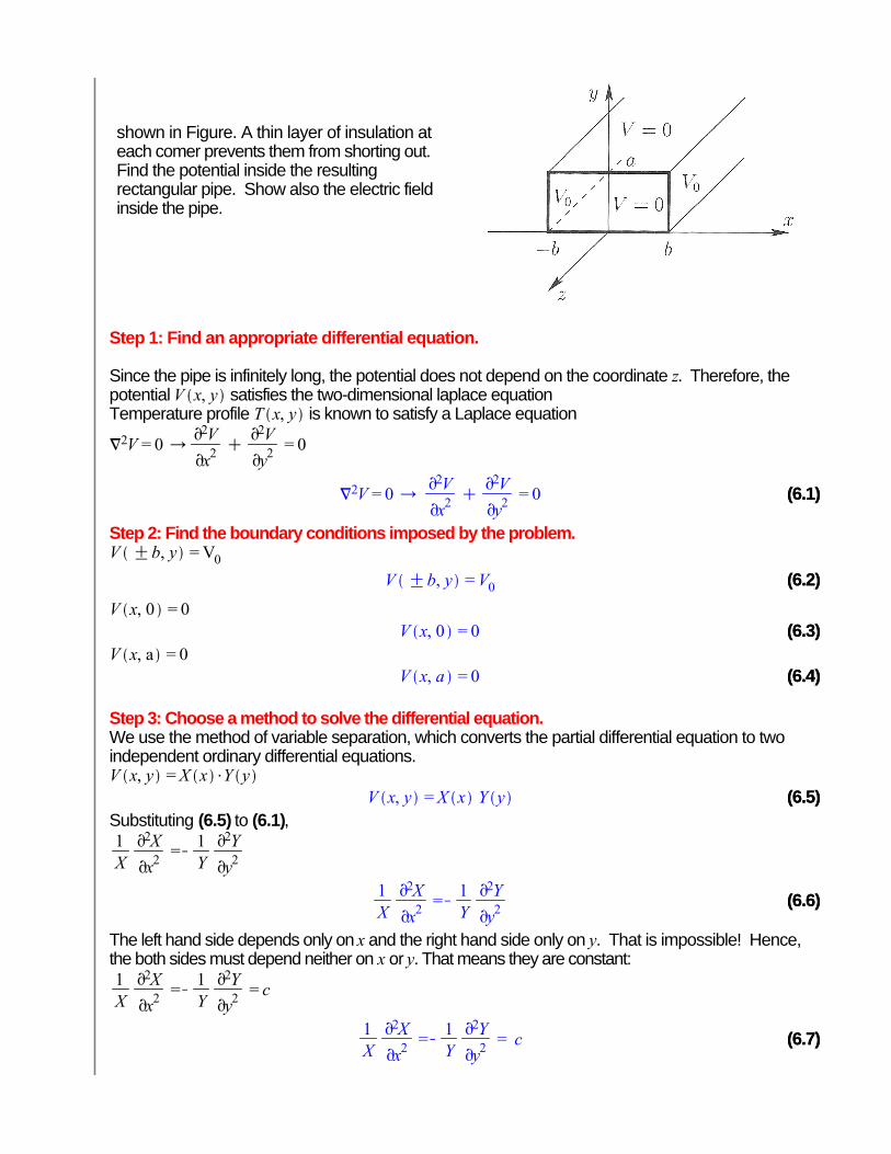
shown in Figure. A thin layer of insulation at each comer prevents them from shorting out.Find the potential inside the resulting rectangular pipe. Show also the electric field inside the pipe.

Step 1: Find an appropriate differential equation.

Since the pipe is infinitely long, the potential does not depend on the coordinate . Therefore, the potential satisfies the two-dimensional laplace equationTemperature profile is known to satisfy a Laplace equation

Step 2: Find the boundary conditions imposed by the problem.

Step 3: Choose a method to solve the differential equation.We use the method of variable separation, which converts the partial differential equation to two independent ordinary differential equations.

Substituting (6.5) to (6.1),

The left hand side depends only on and the right hand side only on . That is impossible! Hence, the both sides must depend neither on or . That means they are constant:

(6.9)(6.9)

(6.11)(6.11)

(6.10)(6.10)

(6.13)(6.13)

(6.14)(6.14)

(6.12)(6.12)

(6.15)(6.15)

(5.15)(5.15)

Then, we have two differential equations:

Step 4: Find general solutions to the ODEs.These equations can be solved analytically. However, the type of solution depends on if ,

, or . Although it is automatically determined by boundary conditions, it is convenient to know the type of solutions before applying the boundary conditions. Since the potential is zero at theboundaries in the direction, it will be convenient to have basis functions that can take zero. When

, is oscillatory and can take zero. So, we assume that . Then, the solutions to Eqs. (6.9) are

Step 5: Determine the unknown constants by applying the boundary conditions.There are five unknowns, , , , , and . On the other hand, there are only four boundary conditions. Don't worry. You will see.

Equations (6.14) and (6.15) suggest that . Hence, the boundary conditions (6.14) and (6.15) are simply

(6.19)(6.19)

(6.18)(6.18)

(6.17)(6.17)

(6.16)(6.16)

(6.20)(6.20)

(5.15)(5.15)

where

.Noting that Eq. (6.15) is a Fourier series, we can determine as an innerproduct between 1 and basis

function :

which is simplified to

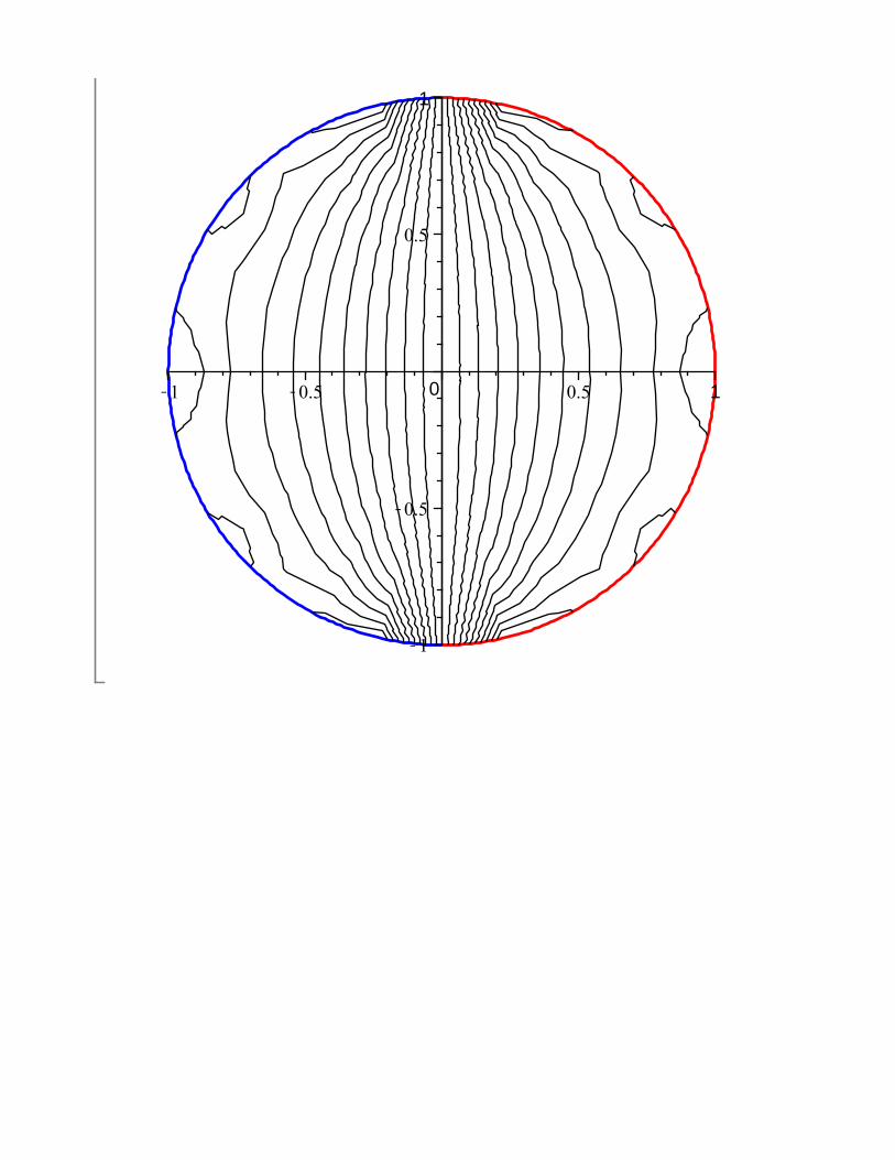
Step 6: Construct the final expression of the solution.

(6.16)(6.16)

(6.21)(6.21)

(5.15)(5.15)

(6.22)(6.22)

(6.16)(6.16)

(6.21)(6.21)

(5.15)(5.15)

(6.22)(6.22)

(6.16)(6.16)

(6.21)(6.21)

(5.15)(5.15)

(6.22)(6.22)

(6.16)(6.16)

(6.21)(6.21)

(5.15)(5.15)

x0 1

y

1

(6.22)(6.22)

(7.5)(7.5)

(7.1)(7.1)

(7.2)(7.2)

(6.16)(6.16)

(7.4)(7.4)

(7.3)(7.3)

(6.21)(6.21)

(5.15)(5.15)

5.3 Example: Spherical coordinatesA spherical shell of radius with an insulating ring in the plane has its upper hemisphere at potential and its lower hemisphere at . Find the potential inside the sphere.

Step 1: Find an appropriate differential equation.

We use the spherical coordinates.

Step 2: Find the boundary conditions imposed by the problem.

Step 3: Separation of variables

Separating variables, Eq. (7.1) can be written as

At this point, is separated from and . Introducing a separation constant , (7.1) may be split to

(7.13)(7.13)

(7.7)(7.7)

(6.16)(6.16)

(7.11)(7.11)

(6.21)(6.21)

(6.22)(6.22)

(7.10)(7.10)

(7.12)(7.12)

(7.9)(7.9)

(7.8)(7.8)

(5.15)(5.15)

(7.6)(7.6)

Now, we can separate and is given by

and for ,

Step 4: Find general solutions to the ODEs.

Equation (7.5) can be solved immediately and its general solution is

Equation (7.7) can be also solved easily. Using Maple ODE solver,

Therefore, its solution is

Solving Eq. (7.8) needs additional steps. Introducing a new variable , (7.8) becomes

where . (7.12) is nothing but a generalized Legendre equation. Since the solution must be real, the general solution is associate Legendre polynomials

and must be a non-negative integer.

Combining general solutions (7.9), (7.11), and (7.13),

(6.16)(6.16)

(7.18)(7.18)

(7.16)(7.16)

(6.21)(6.21)

(6.22)(6.22)

(7.17)(7.17)

(7.15)(7.15)

(7.14)(7.14)

(5.15)(5.15)

Step 5: Determine the unknown constants by applying the boundary conditions.

Boundary condition at .The potential should not diverge at . Therefore, .

Boundary condition at .From (7.3), first we note that the potential does not depends on . Only satisfies the condition. Therefore, .At this point, the potential is written as

and the boundary condition is

Using the orthogonality of Legendre polynomials

Substituting (7.3)

(7.20)(7.20)

(6.16)(6.16)

(6.21)(6.21)

(6.22)(6.22)

(7.19)(7.19)

(5.15)(5.15)

and using , we obtain the final expression

Step 6: Plotting the results:For plotting purpose, we assume and .

Constructing the expansion coefficients:

Constructing the potential:

Draw the boundaries:

Contour plotting of the potential:

(6.22)(6.22)

(7.19)(7.19)

(6.16)(6.16)

(6.21)(6.21)

(5.15)(5.15)

0 1

1