237
NOTICE OF TRADEMARKS
First time violations of trademark laws carry fines of up to $250,000 and five years in jail. "PTV" is a trademark of Bradley F. Cowan "Price-Time Vector" is a trademark of Bradley F. Cowan
COPYRIGHT
Copyright @ 1993 by Bradley Frank Cowan Copyright @ 1998 by Bradley Frank Cowan
All rights reserved. No part of this work covered by the copyright hereon
may be reproduced or used in any form or by any means -graphic, or
mechanical, including photocopying, taping, or information storage and
retrieval systems - without permission of the author. Any copy of this book issued by the author is sold subject to the condition that it SHALL NOT BY WAY OF TRADE OR OTHERWISE, BE
LENT, RE-SOLD, HIRED OUT, OR OTHERWISE CIRCULATED,
WITHOUT THE AUTHOR'S PRIOR CONSENT, in any form of binding or cover other than that in which it is published, and without a similar condition including this condition being imposed on a subsequent purchaser.
This work is dedicated to my mother, Ruby Charolotte Polhemus Miller,
who never compromised the unconditional love she holds for her
children. Through her love and willingness to sacrifice even the bare
necessities in her life for her children, she provided the respect for life,
the self-confidence, and the determination needed to produce and make
available to the public this material.
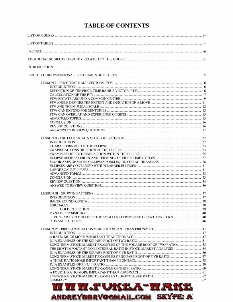
TABLE OF CONTENTS
LIST OF FIGURES ................................................................................................................................................................................... iv LIST OF TABLES.......................................................................................................................................................................................v PREFACE ................................................................................................................................................................................................. vii ADDITIONAL SUBJECTS TO STUDY RELATED TO THIS COURSE.......................................................................................... ix INTRODUCTION .................................................................................................................................................................................... 1 PART I FOUR-DIMENSIONAL PRICE-TIME STRUCTURES....................................................................................................... 5 LESSON I - PRICE-TIME RADII VECTORS (PTV) ........................................................................................................... 6 INTRODUCTION ......................................................................................................................................................... 6 DEFINITION OF THE PRICE-TIME RADIUS VECTOR (PTV)............................................................................. 6 CALCULATION OF THE PTV................................................................................................................................... 7 PTVs ROTATE AROUND A COMMON CENTER ................................................................................................... 9 PTV ANGLE DEFINES THE EXTENT AND DURATION OF A MOVE ............................................................. 11 PTV AND THE MUSICAL SCALE ........................................................................................................................... 12 PTVs CAN EXTEND FOR CENTURIES .................................................................................................................. 13 PTVs CAN OVERLAP AND EXPERIENCE OFFSETS .......................................................................................... 15 ADVANCED TOPICS................................................................................................................................................. 15 CONCLUSION............................................................................................................................................................. 16 REVIEW QUESTIONS ............................................................................................................................................... 16 ANSWERS TO REVIEW QUESTIONS .................................................................................................................... 17 LESSON II - THE ELLIPTICAL NATURE OF PRICE-TIME ........................................................................................... 22 INTRODUCTION ........................................................................................................................................................ 22 CHARACTERISTICS OF THE ELLIPSE.................................................................................................................. 23 GRAPHICAL CONSTRUCTION OF THE ELLIPSE............................................................................................... 23 EXAMPLES OF PRICE-TIME ACTION WITHIN THE ELLIPSE......................................................................... 25 ELLIPSE DEFINES ORIGIN AND TERMINUS OF PRICE-TIME CYCLES ....................................................... 27 MAJOR AXES OF MATED ELLIPSES FORM EQUILATERAL TRIANGLES................................................... 28 ELLIPSES ARE CONTAINED WITHIN LARGER ELLIPSES .............................................................................. 31 LARGE SCALE ELLIPSES ........................................................................................................................................ 31 ADVANCED TOPICS................................................................................................................................................. 33 CONCLUSION............................................................................................................................................................. 33 REVIEW QUESTION.................................................................................................................................................. 34 ANSWER TO REVIEW QUESTION......................................................................................................................... 36 LESSON III - GROWTH PATTERNS.................................................................................................................................. 37 INTRODUCTION ........................................................................................................................................................ 37 BACKGROUND REVIEW ......................................................................................................................................... 38 FIBONACCI ............................................................................................................................................... 38 GOLDEN SECTION ....................................................................................................................................... 39 DYNAMIC SYMMETRY ........................................................................................................................................... 40 FIVE YEAR CYCLE DEFINES THE SMALLEST COMPLETED GROWTH PATTERN................................... 40 ADVANCED TOPICS ................................................................................................................................................ 46 LESSON IV - PRICE-TIME RATIOS MORE IMPORTANT THAN FIBONACCI.......................................................... 47 INTRODUCTION ........................................................................................................................................................ 47 A RATIO MUCH MORE IMPORTANT THAN FIBONACCI ................................................................................ 47 DJIA EXAMPLES OF THE SQUARE ROOT OF TWO RATIO............................................................................. 51 LONG-TERM STOCK MARKET EXAMPLES OF THE SQUARE ROOT OF TWO RATIO............................. 53 THE MOST IMPORTANT NON-INTEGRAL RATIO IN STOCK MARKET ANALYSIS ................................. 54 DJIA EXAMPLES OF THE SQUARE ROOT OF FIVE RATIO ............................................................................. 56 LONG-TERM STOCK MARKET EXAMPLES OF SQUARE ROOT OF FIVE RATIO ...................................... 57 A THIRD RATIO MORE IMPORTANT THAN FIBONNACI................................................................................ 58 DJIA EXAMPLES OF PI (3.14) RATIO .................................................................................................................... 59 LONG-TERM STOCK MARKET EXAMPLE OF THE PI RATIO......................................................................... 60 A FOURTH RATIO MORE IMPORTANT THAN FIBONNACI............................................................................ 61 LONG-TERM STOCK MARKET EXAMPLES OF ROOT THREE RATIO.......................................................... 62 SUMMARY ............................................................................................................................................................... 62
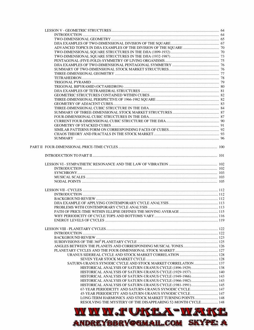
LESSON V - GEOMETRIC STRUCTURES........................................................................................................................ 64 INTRODUCTION ........................................................................................................................................................ 64 TWO-DIMENSIONAL GEOMETRY ........................................................................................................................ 65 DJIA EXAMPLES OF TWO-DIMENSIONAL DIVISION OF THE SQUARE...................................................... 67 ADVANCED TOPICS IN DJIA EXAMPLES OF THE DIVISION OF THE SQUARE ........................................ 70 TWO-DIMENSIONAL SQUARE STRUCTURES IN THE DJIA (1899-1932)...................................................... 70 TWO-DIMENSIONAL SQUARE STRUCTURES IN THE DJIA (1932-1987)...................................................... 73 PENTAGONAL (FIVE-FOLD) SYMMETRY OF LIVING ORGANISMS ............................................................ 75 DJIA EXAMPLES OF TWO-DIMENSIONAL PENTAGONAL SYMMETRY .................................................... 76 SUMMARY OF TWO-DIMENSIONAL STOCK MARKET STRUCTURES........................................................ 76 THREE-DIMENSIONAL GEOMETRY .................................................................................................................... 77 TETRAHEDRON......................................................................................................................................................... 78 TRIGONAL PYRAMID .............................................................................................................................................. 79 TRIGONAL BIPYRAMID (OCTAHEDRON) .......................................................................................................... 80 DJIA EXAMPLES OF TETRAHEDRAL STRUCTURES ....................................................................................... 81 GEOMETRIC STRUCTURES CONTAINED WITHIN CUBES............................................................................. 82 THREE-DIMENSIONAL PERSPECTIVE OF 1966-1982 SQUARE ...................................................................... 82 GEOMETRY OF ADJACENT CUBES...................................................................................................................... 83 THREE-DIMENSIONAL CUBIC STRUCTURE IN THE DJIA.............................................................................. 84 SUMMARY OF THREE-DIMENSIONAL STOCK MARKET STRUCTURES.................................................... 87 FOUR-DIMENSIONAL CUBIC STRUCTURES IN THE DJIA.............................................................................. 87 CURRENT FOUR-DIMENSIONAL CUBIC STRUCTURE OF THE DJIA........................................................... 90 GEOMETRY OF STACKED CUBES........................................................................................................................ 91 SIMILAR PATTERNS FORM ON CORRESPONDING FACES OF CUBES........................................................ 92 CHAOS THEORY AND FRACTALS IN THE STOCK MARKET......................................................................... 93 SUMMARY ............................................................................................................................................................... 96 PART II FOUR-DIMENSIONAL PRICE-TIME CYCLES .............................................................................................................. 100 INTRODUCTION TO PART II ........................................................................................................................................... 101 LESSON VI - SYMPATHETIC RESONANCE AND THE LAW OF VIBRATION ...................................................... 102 INTRODUCTION ...................................................................................................................................................... 102 SYNCHRONY............................................................................................................................................................ 103 MUSICAL SCALES .................................................................................................................................................. 103 NODAL POINTS ....................................................................................................................................................... 105 LESSON VII - CYCLES ....................................................................................................................................................... 112 INTRODUCTION ....................................................................................................................................................... 112 BACKGROUND REVIEW ........................................................................................................................................ 112 DJIA EXAMPLE OF APPLYING CONTEMPORARY CYCLE ANALYSIS....................................................... 113 PROBLEMS WITH CONTEMPORARY CYCLE ANALYSIS .............................................................................. 113 PATH OF PRICE-TIME WITHIN ELLIPSE DEFINES THE MOVING AVERAGE ........................................... 115 WHY PERIODICITY OF CYCLE TOPS AND BOTTOMS VARY....................................................................... 116 ENERGY LEVELS OF CYCLES .............................................................................................................................. 119 LESSON VIII - PLANETARY CYCLES............................................................................................................................. 122 INTRODUCTION ....................................................................................................................................................... 122 BACKGROUND REVIEW ........................................................................................................................................ 123 SUBDIVISIONS OF THE 3600 PLANETARY CYCLE .......................................................................................... 125 ANGLES BETWEEN THE PLANETS AND CORRESPONDING MUSICAL TONES....................................... 126 PLANETARY CYCLES AND THE FOUR-DIMENSIONAL STOCK MARKET................................................ 127 URANUS SIDEREAL CYCLE AND STOCK MARKET CORRELATION........................................... 128 SEVEN YEAR STOCK MARKET CYCLE ................................................................................ 128 SATURN-URANUS SYNODIC CYCLE AND STOCK MARKET CORRELATION........................... 137 HISTORICAL ANALYSIS OF SATURN-URANUS CYCLE (1896-1929).............................. 138 HISTORICAL ANALYSIS OF SATURN-URANUS CYCLE (1929-1937).............................. 140 HISTORICAL ANALYSIS OF SATURN-URANUS CYCLE (1949-1966).............................. 143 HISTORICAL ANALYSIS OF SATURN-URANUS CYCLE (1966-1982).............................. 143 HISTORICAL ANALYSIS OF SATURN-URANUS CYCLE (1981-1991).............................. 145 67-YEAR PERIODICITY AND SATURN-URANUS SYNODIC CYCLE............................... 147 45-YEAR PERIODICITY AND SATURN-URANUS SYNODIC CYCLE............................... 147 LONG-TERM HARMONICS AND STOCK MARKET TURNING POINTS.......................... 148 RESOLVING THE MYSTERY OF THE DISAPPEARING 52-MONTH CYCLE................... 148
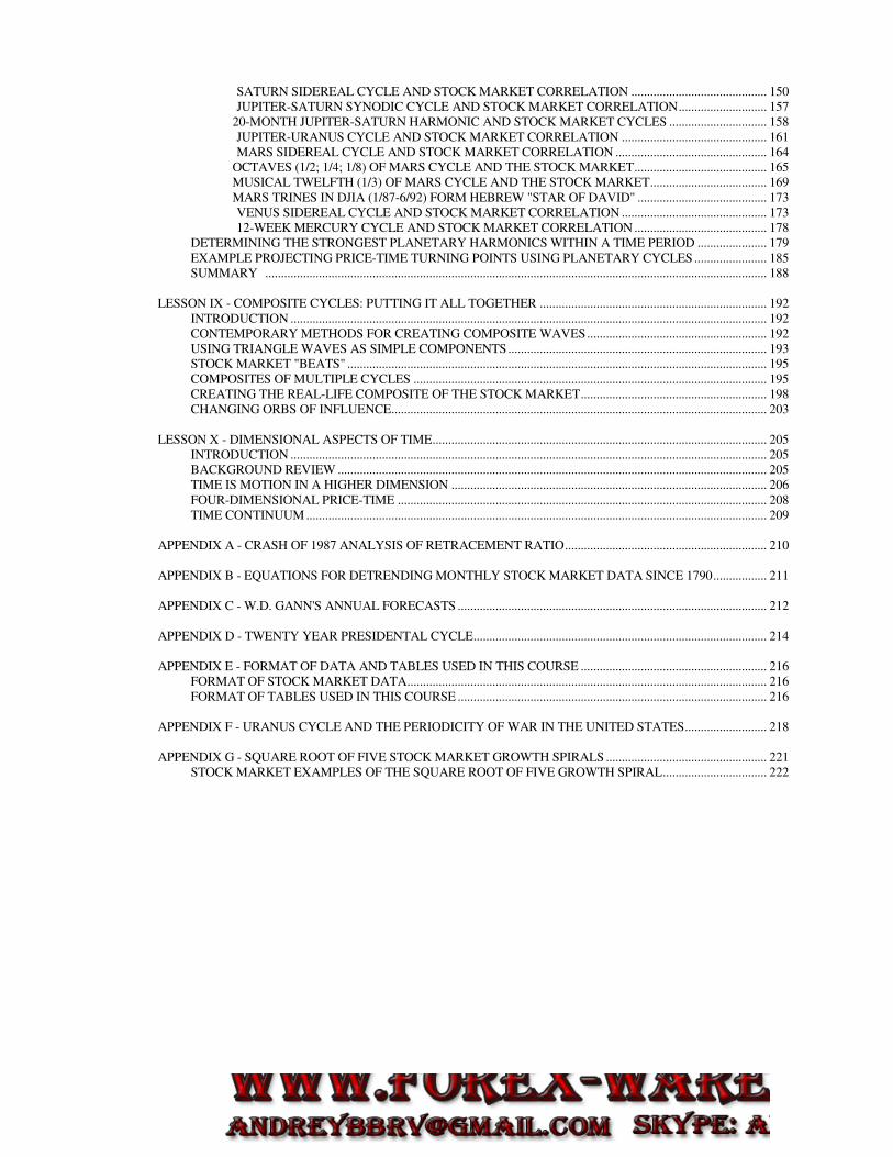
SATURN SIDEREAL CYCLE AND STOCK MARKET CORRELATION ........................................... 150 JUPITER-SATURN SYNODIC CYCLE AND STOCK MARKET CORRELATION............................ 157 20-MONTH JUPITER-SATURN HARMONIC AND STOCK MARKET CYCLES ............................... 158 JUPITER-URANUS CYCLE AND STOCK MARKET CORRELATION .............................................. 161 MARS SIDEREAL CYCLE AND STOCK MARKET CORRELATION ................................................ 164 OCTAVES (1/2; 1/4; 1/8) OF MARS CYCLE AND THE STOCK MARKET.......................................... 165 MUSICAL TWELFTH (1/3) OF MARS CYCLE AND THE STOCK MARKET..................................... 169 MARS TRINES IN DJIA (1/87-6/92) FORM HEBREW "STAR OF DAVID" ......................................... 173 VENUS SIDEREAL CYCLE AND STOCK MARKET CORRELATION .............................................. 173 12-WEEK MERCURY CYCLE AND STOCK MARKET CORRELATION .......................................... 178 DETERMINING THE STRONGEST PLANETARY HARMONICS WITHIN A TIME PERIOD ...................... 179 EXAMPLE PROJECTING PRICE-TIME TURNING POINTS USING PLANETARY CYCLES ....................... 185 SUMMARY ............................................................................................................................................................... 188 LESSON IX - COMPOSITE CYCLES: PUTTING IT ALL TOGETHER ........................................................................ 192 INTRODUCTION ....................................................................................................................................................... 192 CONTEMPORARY METHODS FOR CREATING COMPOSITE WAVES......................................................... 192 USING TRIANGLE WAVES AS SIMPLE COMPONENTS.................................................................................. 193 STOCK MARKET "BEATS" ..................................................................................................................................... 195 COMPOSITES OF MULTIPLE CYCLES ................................................................................................................ 195 CREATING THE REAL-LIFE COMPOSITE OF THE STOCK MARKET........................................................... 198 CHANGING ORBS OF INFLUENCE....................................................................................................................... 203 LESSON X - DIMENSIONAL ASPECTS OF TIME.......................................................................................................... 205 INTRODUCTION ....................................................................................................................................................... 205 BACKGROUND REVIEW ........................................................................................................................................ 205 TIME IS MOTION IN A HIGHER DIMENSION .................................................................................................... 206 FOUR-DIMENSIONAL PRICE-TIME ..................................................................................................................... 208 TIME CONTINUUM .................................................................................................................................................. 209 APPENDIX A - CRASH OF 1987 ANALYSIS OF RETRACEMENT RATIO................................................................ 210 APPENDIX B - EQUATIONS FOR DETRENDING MONTHLY STOCK MARKET DATA SINCE 1790................. 211 APPENDIX C - W.D. GANN'S ANNUAL FORECASTS .................................................................................................. 212 APPENDIX D - TWENTY YEAR PRESIDENTAL CYCLE............................................................................................. 214 APPENDIX E - FORMAT OF DATA AND TABLES USED IN THIS COURSE ........................................................... 216 FORMAT OF STOCK MARKET DATA.................................................................................................................. 216 FORMAT OF TABLES USED IN THIS COURSE .................................................................................................. 216 APPENDIX F - URANUS CYCLE AND THE PERIODICITY OF WAR IN THE UNITED STATES.......................... 218 APPENDIX G - SQUARE ROOT OF FIVE STOCK MARKET GROWTH SPIRALS ................................................... 221 STOCK MARKET EXAMPLES OF THE SQUARE ROOT OF FIVE GROWTH SPIRAL................................. 222
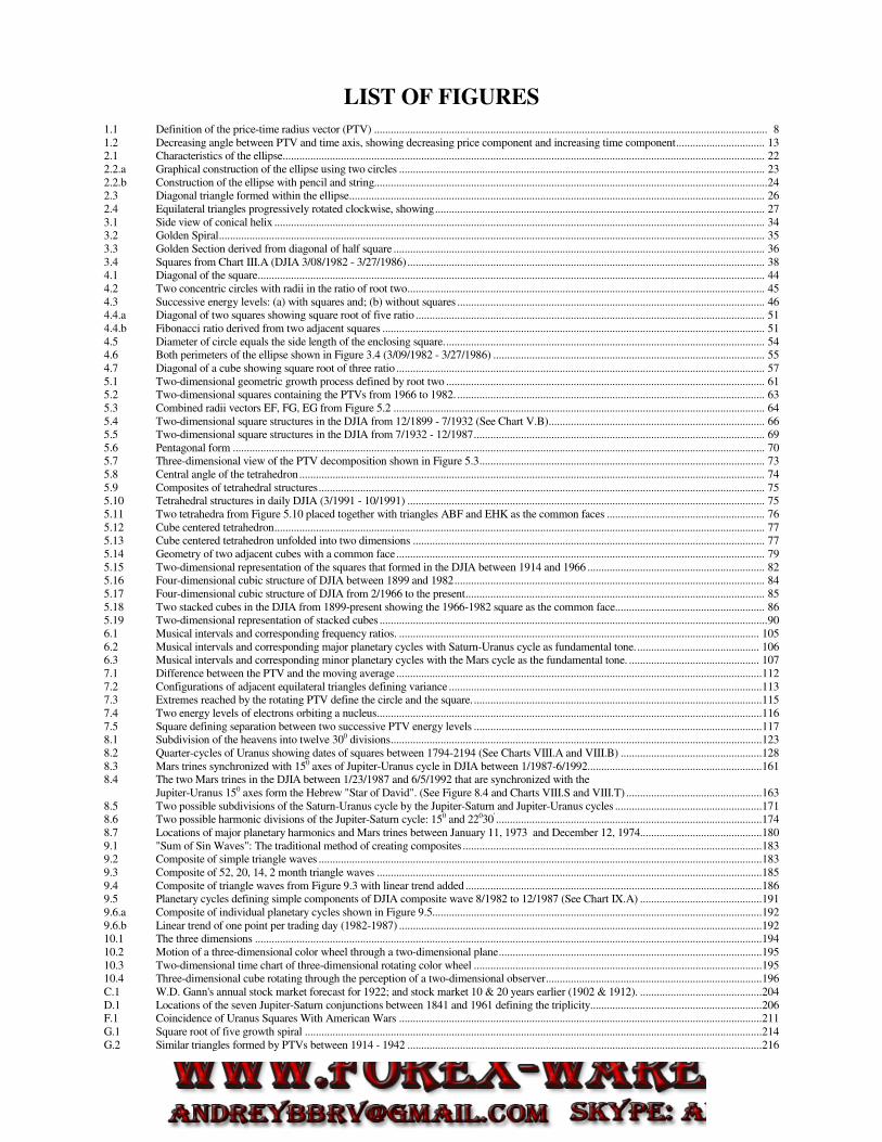
LIST OF FIGURES 1.1 Definition of the price-time radius vector (PTV) .............................................................................................................................................. 8 1.2 Decreasing angle between PTV and time axis, showing decreasing price component and increasing time component................................ 13 2.1 Characteristics of the ellipse.............................................................................................................................................................................. 22 2.2.a Graphical construction of the ellipse using two circles .................................................................................................................................... 23 2.2.b Construction of the ellipse with pencil and string..............................................................................................................................................24 2.3 Diagonal triangle formed within the ellipse...................................................................................................................................................... 26 2.4 Equilateral triangles progressively rotated clockwise, showing....................................................................................................................... 27 3.1 Side view of conical helix ................................................................................................................................................................................. 34 3.2 Golden Spiral..................................................................................................................................................................................................... 35 3.3 Golden Section derived from diagonal of half square ...................................................................................................................................... 36 3.4 Squares from Chart III.A (DJIA 3/08/1982 - 3/27/1986)................................................................................................................................. 38 4.1 Diagonal of the square....................................................................................................................................................................................... 44 4.2 Two concentric circles with radii in the ratio of root two................................................................................................................................. 45 4.3 Successive energy levels: (a) with squares and; (b) without squares ............................................................................................................... 46 4.4.a Diagonal of two squares showing square root of five ratio .............................................................................................................................. 51 4.4.b Fibonacci ratio derived from two adjacent squares .......................................................................................................................................... 51 4.5 Diameter of circle equals the side length of the enclosing square.................................................................................................................... 54 4.6 Both perimeters of the ellipse shown in Figure 3.4 (3/09/1982 - 3/27/1986) .................................................................................................. 55 4.7 Diagonal of a cube showing square root of three ratio ..................................................................................................................................... 57 5.1 Two-dimensional geometric growth process defined by root two ................................................................................................................... 61 5.2 Two-dimensional squares containing the PTVs from 1966 to 1982. ............................................................................................................... 63 5.3 Combined radii vectors EF, FG, EG from Figure 5.2 ...................................................................................................................................... 64 5.4 Two-dimensional square structures in the DJIA from 12/1899 - 7/1932 (See Chart V.B).............................................................................. 66 5.5 Two-dimensional square structures in the DJIA from 7/1932 - 12/1987......................................................................................................... 69 5.6 Pentagonal form ................................................................................................................................................................................................ 70 5.7 Three-dimensional view of the PTV decomposition shown in Figure 5.3....................................................................................................... 73 5.8 Central angle of the tetrahedron........................................................................................................................................................................ 74 5.9 Composites of tetrahedral structures................................................................................................................................................................. 75 5.10 Tetrahedral structures in daily DJIA (3/1991 - 10/1991) ................................................................................................................................. 75 5.11 Two tetrahedra from Figure 5.10 placed together with triangles ABF and EHK as the common faces ......................................................... 76 5.12 Cube centered tetrahedron................................................................................................................................................................................. 77 5.13 Cube centered tetrahedron unfolded into two dimensions ............................................................................................................................... 77 5.14 Geometry of two adjacent cubes with a common face..................................................................................................................................... 79 5.15 Two-dimensional representation of the squares that formed in the DJIA between 1914 and 1966 ................................................................ 82 5.16 Four-dimensional cubic structure of DJIA between 1899 and 1982................................................................................................................ 84 5.17 Four-dimensional cubic structure of DJIA from 2/1966 to the present............................................................................................................ 85 5.18 Two stacked cubes in the DJIA from 1899-present showing the 1966-1982 square as the common face...................................................... 86 5.19 Two-dimensional representation of stacked cubes ............................................................................................................................................90 6.1 Musical intervals and corresponding frequency ratios. .................................................................................................................................. 105 6.2 Musical intervals and corresponding major planetary cycles with Saturn-Uranus cycle as fundamental tone............................................. 106 6.3 Musical intervals and corresponding minor planetary cycles with the Mars cycle as the fundamental tone. ............................................... 107 7.1 Difference between the PTV and the moving average ....................................................................................................................................112 7.2 Configurations of adjacent equilateral triangles defining variance .................................................................................................................113 7.3 Extremes reached by the rotating PTV define the circle and the square.........................................................................................................115 7.4 Two energy levels of electrons orbiting a nucleus...........................................................................................................................................116 7.5 Square defining separation between two successive PTV energy levels ........................................................................................................117 8.1 Subdivision of the heavens into twelve 300 divisions......................................................................................................................................123 8.2 Quarter-cycles of Uranus showing dates of squares between 1794-2194 (See Charts VIII.A and VIII.B) ...................................................128 8.3 Mars trines synchronized with 150 axes of Jupiter-Uranus cycle in DJIA between 1/1987-6/1992...............................................................161 8.4 The two Mars trines in the DJIA between 1/23/1987 and 6/5/1992 that are synchronized with the Jupiter-Uranus 150 axes form the Hebrew "Star of David". (See Figure 8.4 and Charts VIII.S and VIII.T) .................................................163 8.5 Two possible subdivisions of the Saturn-Uranus cycle by the Jupiter-Saturn and Jupiter-Uranus cycles .....................................................171 8.6 Two possible harmonic divisions of the Jupiter-Saturn cycle: 150 and 22030' ................................................................................................174 8.7 Locations of major planetary harmonics and Mars trines between January 11, 1973 and December 12, 1974............................................180 9.1 "Sum of Sin Waves": The traditional method of creating composites ............................................................................................................183 9.2 Composite of simple triangle waves ................................................................................................................................................................183 9.3 Composite of 52, 20, 14, 2 month triangle waves ...........................................................................................................................................185 9.4 Composite of triangle waves from Figure 9.3 with linear trend added ...........................................................................................................186 9.5 Planetary cycles defining simple components of DJIA composite wave 8/1982 to 12/1987 (See Chart IX.A) ............................................191 9.6.a Composite of individual planetary cycles shown in Figure 9.5.......................................................................................................................192 9.6.b Linear trend of one point per trading day (1982-1987) ...................................................................................................................................192 10.1 The three dimensions .......................................................................................................................................................................................194 10.2 Motion of a three-dimensional color wheel through a two-dimensional plane...............................................................................................195 10.3 Two-dimensional time chart of three-dimensional rotating color wheel ........................................................................................................195 10.4 Three-dimensional cube rotating through the perception of a two-dimensional observer..............................................................................196 C.1 W.D. Gann's annual stock market forecast for 1922; and stock market 10 & 20 years earlier (1902 & 1912). ............................................204 D.1 Locations of the seven Jupiter-Saturn conjunctions between 1841 and 1961 defining the triplicity..............................................................206 F.1 Coincidence of Uranus Squares With American Wars ...................................................................................................................................211 G.1 Square root of five growth spiral .....................................................................................................................................................................214 G.2 Similar triangles formed by PTVs between 1914 - 1942 ................................................................................................................................216
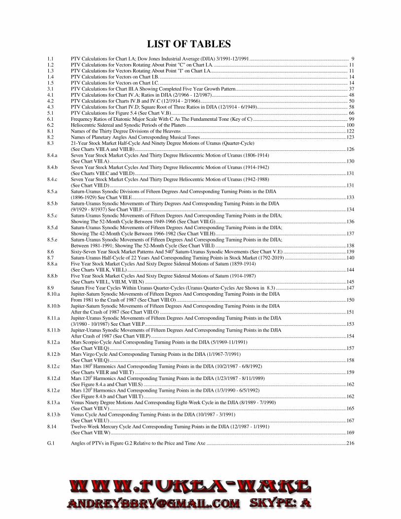
LIST OF TABLES 1.1 PTV Calculations for Chart I.A; Dow Jones Industrial Average (DJIA) 3/1991-12/1991............................................................................... 9 1.2 PTV Calculations for Vectors Rotating About Point "C" on Chart I.A. .......................................................................................................... 11 1.3 PTV Calculations for Vectors Rotating About Point "I" on Chart I.A............................................................................................................. 11 1.4 PTV Calculations for Vectors on Chart I.B. ..................................................................................................................................................... 14 1.5 PTV Calculations for Vectors on Chart I.C. ..................................................................................................................................................... 14 3.1 PTV Calculations for Chart III.A Showing Completed Five Year Growth Pattern......................................................................................... 37 4.1 PTV Calculations for Chart IV.A; Ratios in DJIA (2/1966 - 12/1987)............................................................................................................ 48 4.2 PTV Calculations for Charts IV.B and IV.C (12/1914 - 2/1966)..................................................................................................................... 50 4.3 PTV Calculations for Chart IV.D; Square Root of Three Ratios in DJIA (12/1914 - 6/1949)........................................................................ 58 5.1 PTV Calculations for Figure 5.4 (See Chart V.B)............................................................................................................................................ 66 6.1 Frequency Ratios of Diatonic Major Scale With C As The Fundamental Tone (Key of C) ........................................................................... 99 6.2 Heliocentric Sidereal and Synodic Periods of the Planets.............................................................................................................................. 100 8.1 Names of the Thirty Degree Divisions of the Heavens ...................................................................................................................................122 8.2 Names of Planetary Angles And Corresponding Musical Tones....................................................................................................................123 8.3 21-Year Stock Market Half-Cycle And Ninety Degree Motions of Uranus (Quarter-Cycle) (See Charts VIII.A and VIII.B)........................................................................................................................................................................126 8.4.a Seven Year Stock Market Cycles And Thirty Degree Heliocentric Motion of Uranus (1806-1914) (See Chart VIII.A)............................................................................................................................................................................................130 8.4.b Seven Year Stock Market Cycles And Thirty Degree Heliocentric Motion of Uranus (1914-1942) (See Charts VIII.C and VIII.D)........................................................................................................................................................................131 8.4.c Seven Year Stock Market Cycles And Thirty Degree Heliocentric Motion of Uranus (1942-1988) (See Chart VIII.D)............................................................................................................................................................................................131 8.5.a Saturn-Uranus Synodic Divisions of Fifteen Degrees And Corresponding Turning Points in the DJIA (1896-1929) See Chart VIII.E..........................................................................................................................................................................133 8.5.b Saturn-Uranus Synodic Movements of Thirty Degrees And Corresponding Turning Points in the DJIA (9/1929 - 8/1937) See Chart VIII.F..................................................................................................................................................................134 8.5.c Saturn-Uranus Synodic Movements of Fifteen Degrees And Corresponding Turning Points in the DJIA; Showing The 52-Month Cycle Between 1949-1966 (See Chart VIII.G)........................................................................................................136 8.5.d Saturn-Uranus Synodic Movements of Fifteen Degrees And Corresponding Turning Points in the DJIA; Showing The 42-Month Cycle Between 1966-1982 (See Chart VIII.H)........................................................................................................137 8.5.e Saturn-Uranus Synodic Movements of Fifteen Degrees And Corresponding Turning Points in the DJIA; Between 1981-1991; Showing The 52-Month Cycle (See Chart VIII.I) ........................................................................................................138 8.6 Sixty-Seven Year Stock Market Patterns And 5400 Saturn-Uranus Synodic Movements (See Chart V.E) ..................................................139 8.7 Saturn-Uranus Half-Cycle of 22 Years And Corresponding Turning Points in Stock Market (1792-2019) .................................................140 8.8.a Five Year Stock Market Cycles And Sixty Degree Sidereal Motions of Saturn (1859-1914) (See Charts VIII.K, VIII.L)..............................................................................................................................................................................144 8.8.b Five Year Stock Market Cycles And Sixty Degree Sidereal Motions of Saturn (1914-1987) (See Charts VIII.L, VIII.M, VIII.N) ................................................................................................................................................................145 8.9 Saturn Five Year Cycles Within Uranus Quarter-Cycles (Uranus Quarter-Cycles Are Shown in 8.3) ........................................................147 8.10.a Jupiter-Saturn Synodic Movements of Fifteen Degrees And Corresponding Turning Points in the DJIA From 1981 to the Crash of 1987 (See Chart VIII.O).......................................................................................................................................150 8.10.b Jupiter-Saturn Synodic Movements of Fifteen Degrees And Corresponding Turning Points in the DJIA After the Crash of 1987 (See Chart VIII.O) ....................................................................................................................................................151 8.11.a Jupiter-Uranus Synodic Movements of Fifteen Degrees And Corresponding Turning Points in the DJIA (3/1980 - 10/1987) See Chart VIII.P................................................................................................................................................................153 8.11.b Jupiter-Uranus Synodic Movements of Fifteen Degrees And Corresponding Turning Points in the DJIA After Crash of 1987 (See Chart VIII.P) ...........................................................................................................................................................154 8.12.a Mars Scorpio Cycle And Corresponding Turning Points in the DJIA (5/1969-11/1991) (See Chart VIII.Q)............................................................................................................................................................................................157 8.12.b Mars Virgo Cycle And Corresponding Turning Points in the DJIA (1/1967-7/1991) (See Chart VIII.Q)............................................................................................................................................................................................158 8.12.c Mars 1800 Harmonics And Corresponding Turning Points in the DJIA (10/2/1987 - 6/8/1992) (See Charts VIII.R and VIII.T) ........................................................................................................................................................................159 8.12.d Mars 1200 Harmonics And Corresponding Turning Points in the DJIA (1/23/1987 - 8/11/1989) (See Figure 8.4.a and Chart VIII.S) .................................................................................................................................................................162 8.12.e Mars 1200 Harmonics And Corresponding Turning Points in the DJIA (1/3/1990 - 6/5/1992) (See Figure 8.4.b and Chart VIII.T).................................................................................................................................................................162 8.13.a Venus Ninety Degree Motions And Corresponding Eight-Week Cycle in the DJIA (8/1989 - 7/1990) (See Chart VIII.V)............................................................................................................................................................................................165 8.13.b Venus Cycle And Corresponding Turning Points in the DJIA (10/1987 - 3/1991) (See Chart VIII.U)............................................................................................................................................................................................167 8.14 Twelve-Week Mercury Cycle And Corresponding Turning Points in the DJIA (12/1987 - 1/1991) (See Chart VIII.W)...........................................................................................................................................................................................169
G.1 Angles of PTVs in Figure G.2 Relative to the Price and Time Axe ...............................................................................................................216

ADDITIONAL SUBJECTS TO STUDY
RELATING TO THIS COURSE
W.D. Gann's "Master Course for Stocks" And “Master Course for Commodities”
These courses are actually a series of courses offered by W.D. Gann from 1935 to
1955. To the novice they appear nebulous. However, with this course many of the
things about which Mr. Gann wrote will become clear.
Contemporary Methods of Cycle Analysis
Although these techniques are primitive, they provide a basic foundation upon
which to build. The work by the Foundation for the Study of Cycles is a good
starting point.
Radii Vectors
Review what radii vectors are and how to derive them.
Musical Scales
Study how the "Diatonic Major" scale is constructed; including the frequency
relationships between successive tones in the musical scale as well as to the
fundamental tone.
The same simple mathematical ratios found in sounds that are pleasing to the
human ear are also present in another reflection of human activity, financial
markets.
Patterns in Nature
Naturally occurring phenomena unfold in a limited number of recurring patterns.
These patterns differ between living organisms and inanimate, statically
symmetrical, objects.
Fibonacci Number Series
Although the terminal points of stock market growth patterns are defined by a root
five geometric relationship, it is helpful to understand Fibonacci to gain a basic
understanding of the internals of this growth process.
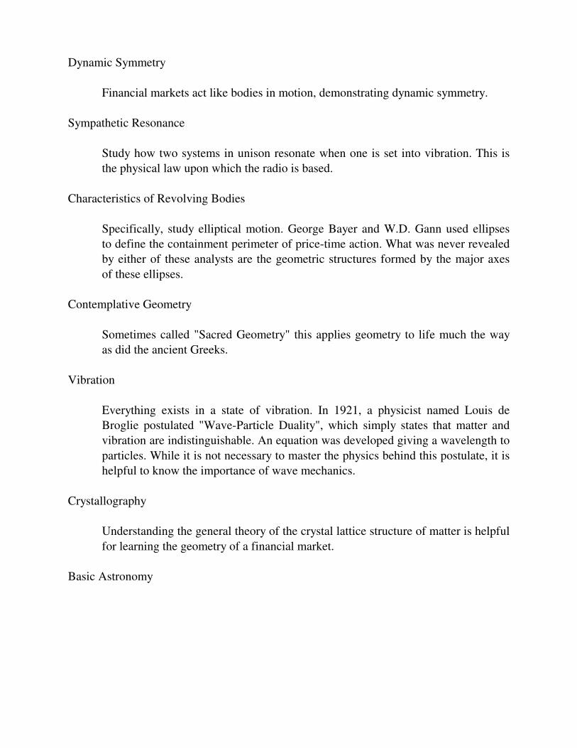
Dynamic Symmetry
Financial markets act like bodies in motion, demonstrating dynamic symmetry.
Sympathetic Resonance
Study how two systems in unison resonate when one is set into vibration. This is
the physical law upon which the radio is based.
Characteristics of Revolving Bodies
Specifically, study elliptical motion. George Bayer and W.D. Gann used ellipses
to define the containment perimeter of price-time action. What was never revealed
by either of these analysts are the geometric structures formed by the major axes
of these ellipses.
Contemplative Geometry
Sometimes called "Sacred Geometry" this applies geometry to life much the way
as did the ancient Greeks.
Vibration
Everything exists in a state of vibration. In 1921, a physicist named Louis de
Broglie postulated "Wave-Particle Duality", which simply states that matter and
vibration are indistinguishable. An equation was developed giving a wavelength to
particles. While it is not necessary to master the physics behind this postulate, it is
helpful to know the importance of wave mechanics.
Crystallography
Understanding the general theory of the crystal lattice structure of matter is helpful
for learning the geometry of a financial market.
Basic Astronomy
PREFACE
The 1998 edition differs from the 1993 in that references were added and a few
typographical errors were corrected. The reader will notice two reference types,
“Technical References” are typically those of college or graduate level science or
engineering. “References” require no technical background. A reference list is provided
in the back.
Previous researchers of financial markets have uncovered pieces of the puzzle behind
the nature of financial market activity. However, either they did not put all these pieces
together, or they chose to not present their knowledge to the public. Because these
researchers made contributions which must be acknowledged,
IT IS THE AUTHOR'S INTENTION THROUGHOUT THIS COURSE
TO GIVE CREDIT FOR ANY MATERIAL THAT HAS BEEN
PREVIOUSLY PRESENTED BY ANOTHER AUTHOR.
Two books are provided with this course. The first book contains written text
describing charts, contained in the second book. Two books allow the reader to have the
charts and the descriptions in front of him at the same time without flipping forward and
backward in the book looking for charts.
It is necessary for the reader to keep the chart under study in front of him. Without
referencing the charts the written text will make little sense.
Even though the concepts presented in this course are not difficult, they will not be
entirely understood with a single reading. It is such a new approach to market analysis that it
takes a little practice to adjust thinking in such a way to fully comprehend what is presented.
It is recommended the reader pass over information he initially finds confusing. When
rereading the course many things will be seen that were missed the first or second time
through.
INTRODUCTION
Financial markets provide a unique laboratory to study the free expression of
human nature with the opportunity to see man pressed to his extreme emotions of hope,
fear, and greed. These extreme emotional swings have been recorded for centuries in the
form of price-time charts.
As man, in mass, is dominated by the feeling of hope, he competes with other
men, bidding prices higher and higher until the dominant emotional mood swings to fear,
which leads to financial market panics.
This course shows how these dominant emotional swings can be forecast well into
the future and, ultimately, provides illumination into their nature and cause. These swings
are present throughout all human activity, but are uniquely expressed and recorded in
financial markets.
THERE ARE NO RANDOM MOTIONS IN FINANCIAL MARKETS. All
ups and downs, twists and turns, booms and crashes follow clear, easy to understand,
natural laws, which can be represented and modeled with applications of basic science.
Libraries around the country are filled with books on financial market analysis,
which basically cover the same worn out subjects. They can all be placed into one of
three categories:
(1) Fundamental analysis
(2) Technical analysis
(3) Cycle analysis
And within the category of technical analysis either they use momentum
indicators, relative strength indexes (RSI), pattern recognition, Elliott Waves, trend lines,
stochastics, or some other subject that has been beaten to death over the years by
hundreds of authors and analysts. All these techniques and many more have been
thoroughly studied by the author and found to have limited value. And few provide any
insight into what is truly happening in financial market activity.
The author's intention in producing this course is to provide unique material to
students of mass human behavior who find the currently available material on this subject
not only lacking dependability and applicability, but also without insight into its true
driving forces. The goal has been to produce an original source of financial market
analysis, and provide it at a price affordable to anyone genuinely interested in the
motivating forces behind human behavior.
This course is the result of over ten years of full time research into financial
market timing and many thousands of dollars devoted to researching the subject material
presented. In addition, over a year was spent by the author compiling the data and writing
2 Four-Dimensional Stock Market Structures And Cycles
this course. The material presented here is UNIQUE, POWERFUL, AND IS NOT
AVAILABLE FROM ANY OTHER SOURCE. Not only are many valuable timing
techniques presented, but also insight into the driving forces behind financial market
price-time changes. No one will be able to read this course and say, "I knew all that".
This is not a "get rich quick" scheme. Truly understanding financial markets
requires study and hard work. No one becomes an expert on any subject, including
financial markets, without putting in the required effort. The reader's advantage as a
student of this material is that much of the work has been done for him. For every path
researched that produced results, at least one hundred dead ends were explored.
Remember, most things that relate to an understanding of nature are simple to understand
when presented, but can be very difficult to discover. Einstein's theory of relativity,
E=MC2, is a simple equation, but could you have derived it?
Contrary to claims of many market analysts who charge exorbitant sums for such
things as simple pattern recognition gimmicks, and claim to hold the "secret of the
universe", mastering the subject of financial market analysis requires hard work.
However, the analyst who spends the time to study this course will broaden his base of
knowledge well beyond what he currently knows, regardless of his current level of
expertise. For those who do not want to put in the work, possibly they would be better off
chasing one of those "secret of the universe" gimmicks, or maybe buying lottery tickets.
The works of the great masters throughout time have been researched. While
many of these analysts had great discoveries, for the most part it appears the general rule
has been to keep these discoveries secret and hidden from the public.
There is no mystery to the author's techniques. They are based on simple
application of science and proven natural law. The author does not dance around a
subject with unclear and hidden messages. All material is supported with extensive and
direct examples in financial market charts.
The reader may have noticed that the market forecasters with the most respectable
records rarely come from academia. Rather, their backgrounds often hold a common
thread of the arts. Musicians, especially, seem to have a predisposition for accurate
market timing. The reason for this will become apparent, as the lessons of this course
unfold. People with a special affinity for music are in harmony with the natural laws
governing proportion and ratios, as experienced through sound. These same laws govern
financial market activity as movements divide and subdivide into the same ratios present
in the "Just Diatonic" musical scale. In more ways than one, these market analysts are
"playing the market".
Similarly, artists are talented with a special understanding of proportion and
symmetry experienced through vision. These laws manifest in financial markets as they
Introduction 3
progress through their natural growth patterns, which demonstrate the same dynamic
symmetry the artist employs when he expresses his talent.
Initially, it may not be clear how some of the material presented in this course relates
to financial markets. However, be aware that the author has focused his efforts on providing
only necessary material, while always keeping in mind the words of William Shakespeare,
"Brevity is the soul of wit".
Those topics that may seem irrelevant are in reality intimately tied to the ultimate
goal of understanding mass human behavior as reflected in financial markets. They are
presented to the reader as physical proof of the omnipresence of natural law. Physical laws
that govern the universe, ranging from bodies in motion to the growth of living organisms,
are also present in the price-time action of financial markets. Albert Einstein said, "The only
randomness is the natural law which we do not yet understand". The proof of this is to
follow.
This course is presented in two parts. The first five lessons define Part One and the
last five lessons compose Part Two.
Part One introduces the new concept of multi-dimensional analysis to financial
markets. The tools for viewing markets in more than the traditional two dimensions of price
and time are developed. After these tools are mastered, they are used to identify the true
geometric structures and ratios, which lie at the heart of financial market activity. The
completed geometric solid that formed between 1899 and 1982 is closely analyzed.
Part Two presents a unique method of analyzing financial market cycles. This is not
the traditional cycle analysis currently practiced by many analysts. Rather, the application of
a scientific phenomenon known as sympathetic resonance is used to isolate cyclical
influences in financial markets, focusing on those in the Dow Jones Industrial Averages
(DJIA).
The ten lessons are organized as follows:
Lesson I introduces a new way of looking at financial markets by presenting the
"Price-Time Radius Vector". This vector allows the analyst to work with price and time as a
single unified element. By looking at price-time as a unified element, various spatial
relationships become evident.
Lesson II uses the vectors studied in Lesson I to define axes of ellipses that contain
financial market action.
Lesson III takes the reader through the natural growth process of financial markets.
Many analysts have studied Growth patterns in the past, but none have understood the true
spatial and multi-dimensional relationships necessary to master this topic.
4 Four-Dimensional Stock Market Structures And Cycles
Lesson IV identifies ratios in price-time much more valuable as timing tools than the
celebrated Fibonacci ratio (1.62). These ratios are visible when a multi-dimensional
perspective is applied.
Lesson V puts together the material presented in previous lessons, and identifies the
geometry of the four-dimensional structures hidden in the two-dimensional price-time charts
of the stock market.
Lesson VI presents the scientific concept of sympathetic resonance and identifies
several examples in nature.
Lesson VII describes what a real cycle is, how varying energy levels define the
duration of these cycles, and explains the age-old problem of varying periodicity of cycle
tops and bottoms.
Lesson VIII shows the correlation between motions of planets and cycles in the Dow
Jones Industrial Average.
Lesson IX shows how to add together all the individual influences in the stock
market to arrive at the true composite effect.
Lesson X describes how the multi-dimensional perspective of financial markets
affects the time element of two-dimensional price-time charts. Traditionally, financial
market analysts have incorrectly represented time as a single dimension along the horizontal
axis of the price-time chart. This lesson will show what is truly happening in the dimension
called time.
PART ONE
FOUR-DIMENSIONAL
PRICE-TIME STRUCTURES
LESSON I
PRICE-TIME RADII VECTORS (PTV)
"Gott wurfelt nicht"
God does not play dice Albert Einstein
INTRODUCTION
A variety of techniques attempt to forecast prices in financial markets. However,
relatively few deal with the most important element in financial market timing, i.e., time.
Traditional cycle analysis is the most commonly used of these techniques, but even the
so-called experts on this subject acknowledge the great limitations of their approach.
Cycles (or more correctly, rhythms) tend to suddenly disappear, only to reappear at a later
date with phase shifts from their original pattern. Contemporary cycle analysts cannot
explain why cycles "disappear", why they reappear with a phase shift, and a variety of
other characteristics that will be explained in this course. DEFINITION OF THE PRICE-TIME RADIUS VECTOR (PTV)
1
To begin the analysis of the dimension of time it must be understood that financial market movements are defined within the limits of radii vectors. These vectors allow analysts to expand their thinking beyond one dimension at a time, i.e., only price levels or only time values, and to START VIEWING PRICE-TIME AS A SINGLE UNIFIED
ELEMENT. For, as will be shown in this course, PRICE AND TIME ARE
INTIMATELY CONNECTED.
On a traditional price-time chart of any financial market, the price-time radius
vector is defined as shown in Figure 1.1. For the sake of brevity, the price-time radius
vector will, hereafter, be referred to as PTV.
This is an application of the Pythagorean theorem taught in high school geometry
classes, which states that the sum of the squares of the sides of a right triangle is equal to
the square of the hypotenuse. In this case, the sides of the right triangle are time and
price, and the hypotenuse is the PTV. 2
1
Please note that "PTV" and "Price-Time Vector" are registered trademarks. 2 The concept of applying the Pythagorean Theorem to price and time simultaneously was
discovered by the author.
For those without a scientific background, a radius vector simply measures the distance and
direction from one point in space to another point in space. On price-time charts of financial
markets, a point in space is a specific price at a specific time. For example, if stock XYZ traded at
33 on January 14th, that would be a point in space on a price-time chart.
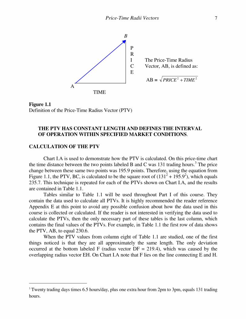
Price-Time Radii Vectors 7
B
P
R
I The Price-Time Radius C Vector, AB, is defined as: E
AB = 22TIMEPRICE +
A TIME
Figure 1.1
Definition of the Price-Time Radius Vector (PTV)
THE PTV HAS CONSTANT LENGTH AND DEFINES THE INTERVAL OF OPERATION WITHIN SPECIFIED MARKET CONDITIONS.
CALCULATION OF THE PTV
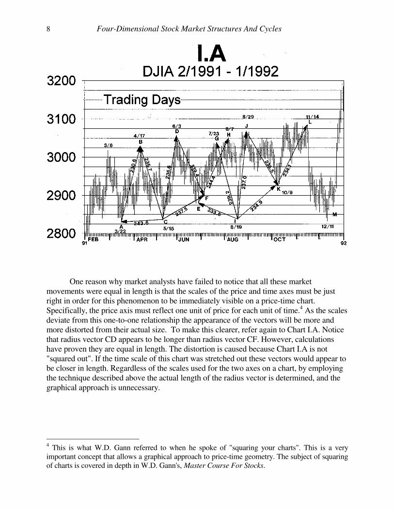
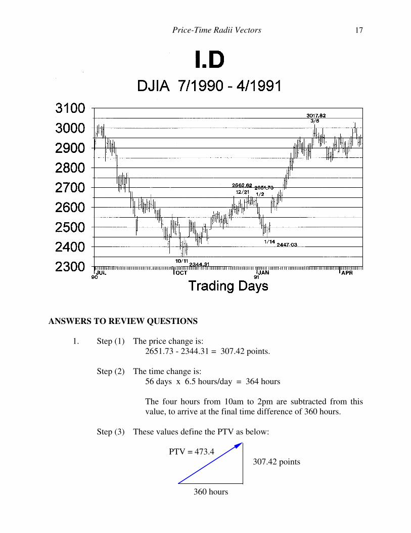
Chart I.A is used to demonstrate how the PTV is calculated. On this price-time chart the time distance between the two points labeled B and C was 131 trading hours.3 The price change between these same two points was 195.9 points. Therefore, using the equation from Figure 1.1, the PTV, BC, is calculated to be the square root of (1312 + 195.92), which equals 235.7. This technique is repeated for each of the PTVs shown on Chart I.A, and the results are contained in Table 1.1. Tables similar to Table 1.1 will be used throughout Part I of this course. They contain the data used to calculate all PTVs. It is highly recommended the reader reference Appendix E at this point to avoid any possible confusion about how the data used in this course is collected or calculated. If the reader is not interested in verifying the data used to calculate the PTVs, then the only necessary part of these tables is the last column, which contains the final values of the PTVs. For example, in Table 1.1 the first row of data shows the PTV, AB, to equal 230.6. When the PTV values from column eight of Table 1.1 are studied, one of the first things noticed is that they are all approximately the same length. The only deviation occurred at the bottom labeled F (radius vector DF = 219.4), which was caused by the overlapping radius vector EH. On Chart I.A note that F lies on the line connecting E and H.
3 Twenty trading days times 6.5 hours/day, plus one extra hour from 2pm to 3pm, equals 131 trading
hours.
8 Four-Dimensional Stock Market Structures And Cycles
One reason why market analysts have failed to notice that all these market movements were equal in length is that the scales of the price and time axes must be just right in order for this phenomenon to be immediately visible on a price-time chart. Specifically, the price axis must reflect one unit of price for each unit of time.4 As the scales deviate from this one-to-one relationship the appearance of the vectors will be more and more distorted from their actual size. To make this clearer, refer again to Chart I.A. Notice that radius vector CD appears to be longer than radius vector CF. However, calculations have proven they are equal in length. The distortion is caused because Chart I.A is not "squared out". If the time scale of this chart was stretched out these vectors would appear to be closer in length. Regardless of the scales used for the two axes on a chart, by employing the technique described above the actual length of the radius vector is determined, and the graphical approach is unnecessary.
4 This is what W.D. Gann referred to when he spoke of "squaring your charts". This is a very important concept that allows a graphical approach to price-time geometry. The subject of squaring of charts is covered in depth in W.D. Gann's, Master Course For Stocks.
Price-Time Radii Vectors 9
Table 1.1
PTV Calculations for Chart I.A
Dow Jones Industrial Average (DJIA) 3/1991-12/1991
Price-
Time
Radius
Vector
Date &
Time
of High
PTV
Price
High
Date &
Time
of Low
PTV
Price
Low
Time
Change
(hours)
Price
Change
(points)
Vector
Value
(PTV)
AB 4/17 2PM
3030.5 3/22 12PM
2829.2 112.5 201.3 230.6
BC 4/17 2PM
3030.5 5/15 3PM
2834.5 131 195.9 235.7
CD 6/03 4PM
3057.5 5/15 3PM
2834.5 79.0 223.0 236.6
DF 6/03 4PM
3057.5 7/08 10AM
2897.4 150 160.1 219.4
EH 8/07 12PM
3050.5 6/28 1PM
2879.3 174.5 171.2 244.4
GI 7/23 10AM
3038.2 8/19 3PM
2836.3 128.5 201.9 239.2
IJ 8/29 10AM
3068.6 8/19 3PM
2836.3 47.0 232.3 237.0
JK 8/29 10AM
3068.6 10/9 3PM
2925.5 187 143.11 235.5
KL 11/14 11AM
3085.0 10/8 1PM
2927.8 173.5 157.2 234.1
PTVs ROTATE AROUND A COMMON CENTER
On Chart I.A the points "C" and "I" hold special significance. These two points represent the center points about which these two radii vectors rotate in a clockwise direction. The "C" radius vector starts with CA, sweeps through CB, over to CD, and finally terminates with CF. The "I" radius vector starts with IE, sweeps through IG, over to IJ, and finally terminates with IK. An interesting concept is that these two rotating radii vectors have their beginning points defined before their center points have been reached in time. For example, at point A the radius vector swinging from A to B is already moving within the limits of the radius vector centered at point C, EVEN THOUGH POINT C HAD YET TO OCCUR IN
TIME.
10 Four-Dimensional Stock Market Structures And Cycles
The following radii vectors are equal length:5 CA = 243.6 CB = 235.7 CD = 236.6 CF = 237.5
The values used for the calculation of these radii vectors are contained within
Table 1.2. Similarly, Table 1.3 shows that the radii vectors rotating around point "I" have
equal lengths:
IE = 233.5
IG = 239.3
IJ = 237.0
IK = 234.9
Table 1.2
PTV Calculations for Vectors
Rotating About Point "C" on Chart I.A.
Price-
Time
Radius
Vector
Date &
Time
of High
PTV
Price
High
Date &
Time
of Low
PTV
Price
Low
Time
Change
(hours)
Price
Change
(points)
Vector
Value
(PTV)
CA 5/15 3PM
2834.5 3/22 12PM
2829.2 243.5 5.3 243.6
CB 4/17 2PM
3030.5 5/15 3PM
2834.5 131.0 195.9 235.7
CD 6/03 4PM
3057.5 5/15 3PM
2834.5 79.0 223 236.6
CF 7/08 10AM
2897.4 5/15 3PM
2834.5 229.0 62.9 237.5
The reason why radius vector DF was shorter than the other vectors is now apparent. The sequence of radii vectors rotating around point C terminated with radius vector CF. However, the radii vectors rotating around point I began with radius vector IE. This means the two cycles overlapped by the amount EF, causing the terminal point of DF to be "pulled up" by the radius vector rotating around point I.
5 These values are equal within the resolution of the intraday data used for their calculation. The non-homogeneous nature of the DJIA index also negatively affects these results.
Price-Time Radii Vectors 11
Table 1.3
PTV Calculations for Vectors
Rotating About Point "I" on Chart I.A.
Price-
Time
Radius
Vector
Date &
Time
of High
PTV
Price
High
Date &
Time
of Low
PTV
Price
Low
Time
Change
(hours)
Price
Change
(points)
Vector
Value
(PTV)
IE 6/28 1PM
2879.3 8/19 3PM
2836.3 229.5 43 233.5
IG 7/23 10AM
3038.2 8/19 3PM
2836.3 128.5 201.9 239.3
IJ 8/29 10AM
3068.7 8/19 3PM
2836.3 47.0 232.34 237.0
IK 10/07 11AM
2926.2 8/19 3PM
2836.3 217.0 89.9 234.9
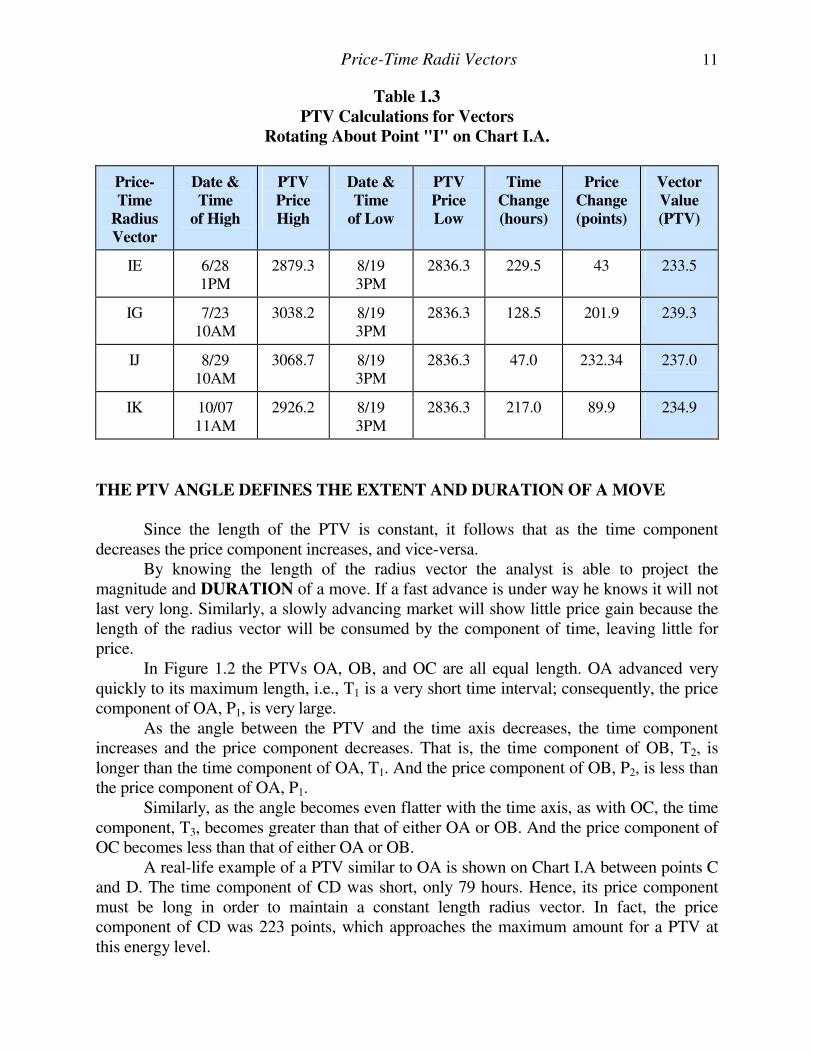
THE PTV ANGLE DEFINES THE EXTENT AND DURATION OF A MOVE
Since the length of the PTV is constant, it follows that as the time component decreases the price component increases, and vice-versa. By knowing the length of the radius vector the analyst is able to project the magnitude and DURATION of a move. If a fast advance is under way he knows it will not last very long. Similarly, a slowly advancing market will show little price gain because the length of the radius vector will be consumed by the component of time, leaving little for price. In Figure 1.2 the PTVs OA, OB, and OC are all equal length. OA advanced very quickly to its maximum length, i.e., T1 is a very short time interval; consequently, the price component of OA, P1, is very large. As the angle between the PTV and the time axis decreases, the time component increases and the price component decreases. That is, the time component of OB, T2, is longer than the time component of OA, T1. And the price component of OB, P2, is less than the price component of OA, P1. Similarly, as the angle becomes even flatter with the time axis, as with OC, the time component, T3, becomes greater than that of either OA or OB. And the price component of OC becomes less than that of either OA or OB. A real-life example of a PTV similar to OA is shown on Chart I.A between points C and D. The time component of CD was short, only 79 hours. Hence, its price component must be long in order to maintain a constant length radius vector. In fact, the price component of CD was 223 points, which approaches the maximum amount for a PTV at this energy level.
12 Four-Dimensional Stock Market Structures And Cycles
An example of a PTV similar to OB is shown on Chart I.A, between points E and H. Between those two points the time component was 174.5 hours. Hence, the price component must be shorter than it was in CD to maintain the constant length radius vector. In fact, the price component was 171.2 points.
PTV AND THE MUSICAL SCALE The frequency of notes on the musical scale are defined by ratios of simple integers relative to the fundamental tone (such as the octave=2:1, the fifth=3:2, the fourth=4:3, etc).6 Similarly, lengths of PTVs are defined by the same ratios as found on the musical scale.
A
P1 P R
I P2 B C E
P3 C
T1 T2 T3
TIME Figure 1.2
Decreasing angle between PTV and the time axis, showing decreasing price component and increasing time component
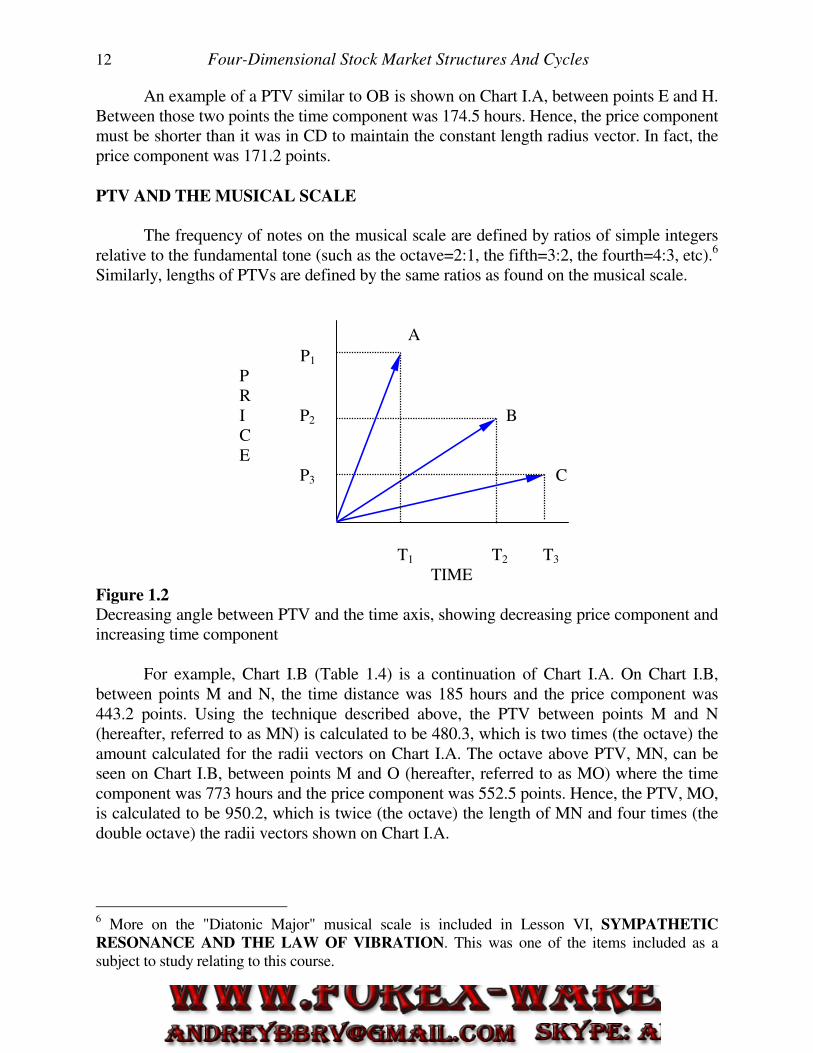
For example, Chart I.B (Table 1.4) is a continuation of Chart I.A. On Chart I.B, between points M and N, the time distance was 185 hours and the price component was 443.2 points. Using the technique described above, the PTV between points M and N (hereafter, referred to as MN) is calculated to be 480.3, which is two times (the octave) the amount calculated for the radii vectors on Chart I.A. The octave above PTV, MN, can be seen on Chart I.B, between points M and O (hereafter, referred to as MO) where the time component was 773 hours and the price component was 552.5 points. Hence, the PTV, MO, is calculated to be 950.2, which is twice (the octave) the length of MN and four times (the double octave) the radii vectors shown on Chart I.A.
6 More on the "Diatonic Major" musical scale is included in Lesson VI, SYMPATHETIC
RESONANCE AND THE LAW OF VIBRATION. This was one of the items included as a subject to study relating to this course.
Price-Time Radii Vectors 13
Table 1.4
PTV Calculations for
Vectors on Chart I.B.
Price-
Time
Radius
Vector
Date &
Time
of High
PTV
Price
High
Date &
Time
of Low
PTV
Price
Low
Time
Change
(hours)
Price
Change
(points)
Vector
Value
(PTV)
MN 1/29 1PM
3313.5 12/18 10AM
2870.3 185 443.2 480.3
MO 6/08 4PM
3422.8 12/18 10AM
2870.3 773 552.5 950.2 = MNx2
PTVs CAN EXTEND FOR CENTURIES
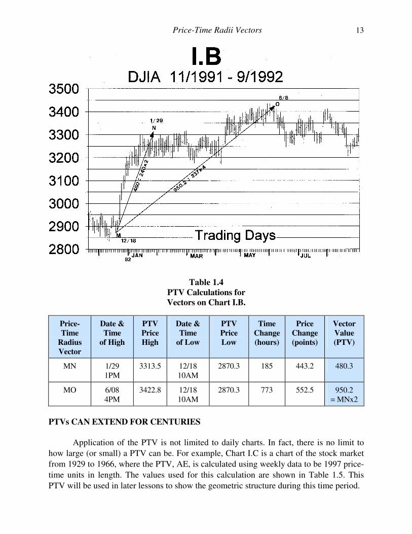
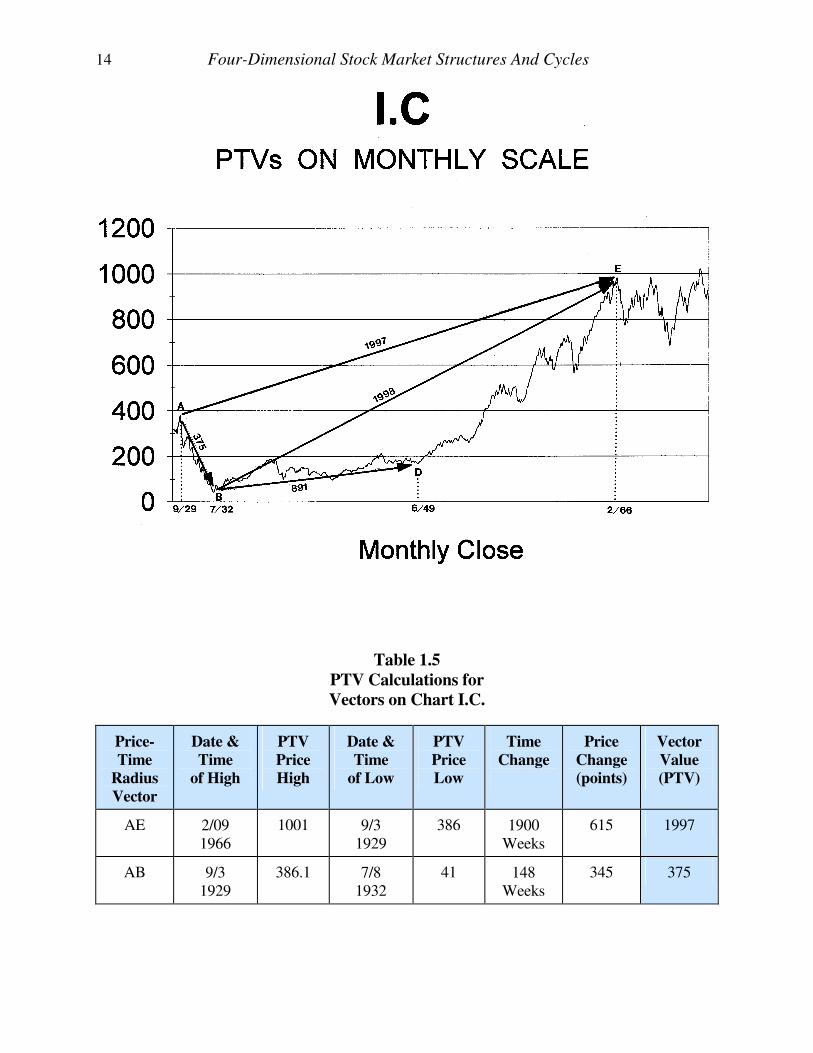
Application of the PTV is not limited to daily charts. In fact, there is no limit to
how large (or small) a PTV can be. For example, Chart I.C is a chart of the stock market
from 1929 to 1966, where the PTV, AE, is calculated using weekly data to be 1997 price-
time units in length. The values used for this calculation are shown in Table 1.5. This
PTV will be used in later lessons to show the geometric structure during this time period.
14 Four-Dimensional Stock Market Structures And Cycles
Table 1.5
PTV Calculations for
Vectors on Chart I.C.
Price-
Time
Radius
Vector
Date &
Time
of High
PTV
Price
High
Date &
Time
of Low
PTV
Price
Low
Time
Change
Price
Change
(points)
Vector
Value
(PTV)
AE 2/09 1966
1001 9/3 1929
386 1900 Weeks
615 1997
AB 9/3 1929
386.1 7/8 1932
41 148 Weeks
345 375
Price-Time Radii Vectors 15
PTVs CAN OVERLAP AND EXPERIENCE OFFSETS
The origin or terminus of a PTV does not necessarily coincide with the origin or
terminus of another PTV. In other words, PTVs can overlap and they can experience
offsets.
An example of overlapping PTVs can be seen on Chart I.A where the PTV
defining the top at point H originated at point E. However, the PTVs preceding EH
terminated at point F. Hence, they overlapped by the amount EF. Similarly, the terminus
of EH overlapped the terminus of IG.
Vertical offsets typically occur with "gaps". Chart I.D is used in the "Review
Questions" section of this lesson. On this chart the origin of the PTV terminating on
3/6/1991 is shown to be the bottom on 1/23/1991, which occurred after the gap on
1/17/1991. The concept of vertical offsets is expanded in Lesson VII, CYCLES.
The possibility that PTVs can overlap and experience offsets complicates the
analysis. However, with practice and experience the precise beginning point of a PTV
can be determined, even if it lies within the field of a previous radius vector. This subject
is covered in greater detail later in this course.
ADVANCED TOPICS
This section is added for those who feel comfortable with an explanation that appears to be more advanced than that encountered in the previous analysis. On Chart I.A since the radii vectors CA, AB, and BC are all equal length, they form three legs of an equilateral triangle.7 In addition, the radii vectors CF, CD, and DF form three legs of another equilateral triangle. These two triangles are contained within the semi-cycle, ABDF. Similarly, the remaining semi-cycle, EHJK, contains two equilateral triangles. The significance of this will be left as an exercise for the reader. But, as a hint, try to find how many equilateral triangles fit into a circle with each leg equal to the radius of the circle. This creates a geometric figure. Students of relativity are familiar with the concept of "curvilinear time", as popularized by Albert Einstein. Traditional charts of financial markets provide an oversimplified two-dimensional representation of what is actually a multi-dimensional phenomenon. Price-time charts simply reflect a "shadow" of this multi-dimensional action. Time is not a linear dimension and hence, cannot be accurately represented by a straight one-dimensional axis across the bottom of a chart.8 When price-time is forced onto a two-dimensional chart, the resultant appearance is that of price-time twisting and turning into and out of the page of observation. The PTV, as described above, allows the analyst to better represent and predict this complicated motion.
7 An equilateral triangle has all three legs equal and the three inner angles equal to 600. 8 Technical Reference: Modern Physics, P. 20 – 21.
16 Four-Dimensional Stock Market Structures And Cycles
Spend a few moments thinking about the time concepts presented in this lesson. As mentioned earlier and repeated here, Chart I.A showed that the price-time action was contained within the radius vector originating at point C. When the market was at point A and moving to point B it was under the influence of a radius vector whose origin at point C had yet to occur in time.
CONCLUSION
It is important the material presented in this lesson is mastered because the following lessons rely heavily on the PTV. At this point in the course the reader should be able to: 1. Determine the PTV between any two points on a price-time chart. 2. Project a price value from any top or bottom given the expected number of
days from that top or bottom. 3. Project when a top or bottom will occur given the dominant resistance or
support level.
REVIEW QUESTIONS
The following questions refer to Chart I.D 1. On 10/11/1990 at 2 pm the DJIA bottomed at 2344.31, intraday. Fifty-six
days later, on 1/2/91 at 10 am, the DJIA reached its top at 2651.73. What is the PTV from this low to high?
2. On 1/14/91 the DJIA bottomed at 2447.03 at 3 pm. What is the PTV from the
top of 2662.62, on 12/21/90 at 3pm, to the low on 1/14/91? 3. On 1/23/91 at 11 am the DJIA bottomed at 2584.65. Your cycle analysis has
advanced to the stage where you expect a significant advance that will top out 29 days later, on 3/6/91. What value will you expect for the DJIA at that time?
4. On 10/11/90 at 2 pm the DJIA bottomed at 2344.31. Your understanding of
resistance levels has advanced to the stage where you can project the DJIA to advance to a value of 3020. What day will this top occur?
5. In 1908 W.D. Gann amazed reporters and traders by stating "Union Pacific will not trade at 169 before it has a good break". At the time of this statement Union Pacific was trading at 168 1/8. Union Pacific did not reach 169. Gann said his ability to make such a statement was based on the "Law of Vibration". Based on the PTV, how could such a statement be made?
Price-Time Radii Vectors 17
ANSWERS TO REVIEW QUESTIONS
1. Step (1) The price change is: 2651.73 - 2344.31 = 307.42 points. Step (2) The time change is: 56 days x 6.5 hours/day = 364 hours
The four hours from 10am to 2pm are subtracted from this value, to arrive at the final time difference of 360 hours.
Step (3) These values define the PTV as below:
PTV = 473.4 307.42 points
360 hours
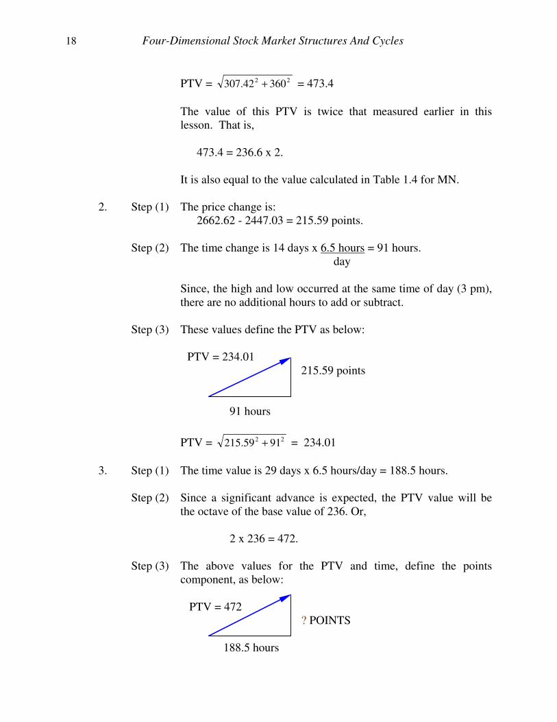
18 Four-Dimensional Stock Market Structures And Cycles
PTV = 22 36042.307 + = 473.4
The value of this PTV is twice that measured earlier in this lesson. That is,
473.4 = 236.6 x 2. It is also equal to the value calculated in Table 1.4 for MN. 2. Step (1) The price change is: 2662.62 - 2447.03 = 215.59 points. Step (2) The time change is 14 days x 6.5 hours = 91 hours. day Since, the high and low occurred at the same time of day (3 pm),
there are no additional hours to add or subtract.
Step (3) These values define the PTV as below:
PTV = 234.01 215.59 points 91 hours
PTV = 22 9159.215 + = 234.01
3. Step (1) The time value is 29 days x 6.5 hours/day = 188.5 hours. Step (2) Since a significant advance is expected, the PTV value will be
the octave of the base value of 236. Or, 2 x 236 = 472. Step (3) The above values for the PTV and time, define the points
component, as below: PTV = 472 ? POINTS 188.5 hours
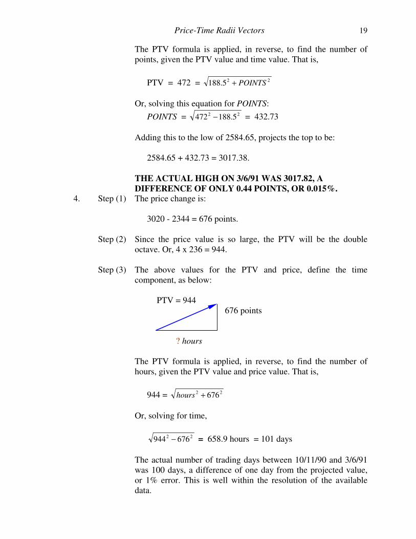
Price-Time Radii Vectors 19
The PTV formula is applied, in reverse, to find the number of points, given the PTV value and time value. That is,
PTV = 472 = 225.188 POINTS+
Or, solving this equation for POINTS:
POINTS = 22 5.188472 − = 432.73
Adding this to the low of 2584.65, projects the top to be: 2584.65 + 432.73 = 3017.38.
THE ACTUAL HIGH ON 3/6/91 WAS 3017.82, A
DIFFERENCE OF ONLY 0.44 POINTS, OR 0.015%. 4. Step (1) The price change is: 3020 - 2344 = 676 points. Step (2) Since the price value is so large, the PTV will be the double
octave. Or, 4 x 236 = 944. Step (3) The above values for the PTV and price, define the time
component, as below: PTV = 944 676 points ? hours The PTV formula is applied, in reverse, to find the number of
hours, given the PTV value and price value. That is,
944 = 22 676+hours
Or, solving for time,
22 676944 − = 658.9 hours = 101 days
The actual number of trading days between 10/11/90 and 3/6/91
was 100 days, a difference of one day from the projected value, or 1% error. This is well within the resolution of the available data.
20 Four-Dimensional Stock Market Structures And Cycles
5. In 1908 when Union Pacific traded at 168 1/8 it was at a point where the PTV from its previous bottom had reached its maximum length, based upon the length of PTVs immediately preceding it. This maximum length was calculated as demonstrated in this lesson. Since the PTV had reached its end, the only direction for the stock to move was down or sideways.


LESSON II
THE ELLIPTICAL NATURE OF PRICE-TIME 9
... there is another kind of curved space, "elliptical space", that excels in its simplicity, since all points in it are equivalent.
Albert Einstein ...The Theory of Relativity
INTRODUCTION
Albert Einstein was known for carefully choosing his words, especially in his writings. In the above quote Einstein did not say that all points in the ellipse are EQUAL. He said all points in the ellipse are EQUIVALENT. Equivalence has special meaning in the world of science. It is recommended the reader reference one of the many sources of modern physics concerning the topic of equivalence. Elliptical motion is consistent throughout nature. The planets move around the sun in elliptical orbits. The sun moves around the galaxy in an elliptical path. The electron moves around the nucleus of the atom in an elliptical orbit. In fact, any body set revolving about a center will assume an elliptical orbit. The circle is a special example of elliptical motion. That is, the circle is an ellipse with eccentricity of zero.10 Lesson I introduced "price-time radii vectors", showed how the length of these vectors are constant, and that their lengths are often integral multiples of smaller vectors. The vector allows the analyst to expand his perspective of financial market charts beyond the single dimensions of price or time. With the PTV, direct measurements can be made from one point of force to another within a two-dimensional plane. Lesson II will explain the nature of these vectors and show that they define the axes of ellipses. The PTV defines the two-dimensional spacing between two points of force. The ellipse defines the potential deviation from this PTV as the price-time action is contained within its perimeter.
PRICE-TIME ACTION IS CONTAINED WITHIN THE PERIMETER
OF ELLIPSES, WHOSE MAJOR AND MINOR AXES ARE "PRICE-
TIME RADII VECTORS".
9 Ellipses were used by a trader, George Bayer, in the San Francisco area shortly after the turn of the century. He wrote a small amount of material about ellipses. The relevant points of his writing are contained within this course. In addition, the concept is greatly advanced beyond anything previously written by any author.
10 For those who are mathematically inclined, the ellipse is represented by the equation, (X2/A2)+(Y2/B2) = 1, where A is the semi-major axis, B is the semi-minor axis, and A2 = B2 + C2. C represents the distance from the center to a focus, and X,Y represents a point on the perimeter.
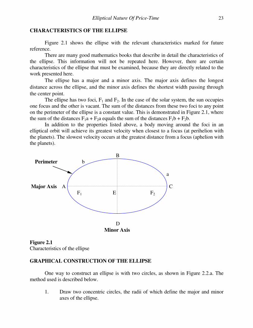
Elliptical Nature Of Price-Time 23
CHARACTERISTICS OF THE ELLIPSE
Figure 2.1 shows the ellipse with the relevant characteristics marked for future reference. There are many good mathematics books that describe in detail the characteristics of the ellipse. This information will not be repeated here. However, there are certain characteristics of the ellipse that must be examined, because they are directly related to the work presented here.
The ellipse has a major and a minor axis. The major axis defines the longest
distance across the ellipse, and the minor axis defines the shortest width passing through
the center point. The ellipse has two foci, F1 and F2. In the case of the solar system, the sun occupies one focus and the other is vacant. The sum of the distances from these two foci to any point on the perimeter of the ellipse is a constant value. This is demonstrated in Figure 2.1, where the sum of the distances F1a + F2a equals the sum of the distances F1b + F2b. In addition to the properties listed above, a body moving around the foci in an elliptical orbit will achieve its greatest velocity when closest to a focus (at perihelion with the planets). The slowest velocity occurs at the greatest distance from a focus (aphelion with the planets). B Perimeter b
a
Major Axis A C
F1 E F2
D Minor Axis
Figure 2.1 Characteristics of the ellipse
GRAPHICAL CONSTRUCTION OF THE ELLIPSE
One way to construct an ellipse is with two circles, as shown in Figure 2.2.a. The method used is described below. 1. Draw two concentric circles, the radii of which define the major and minor
axes of the ellipse.
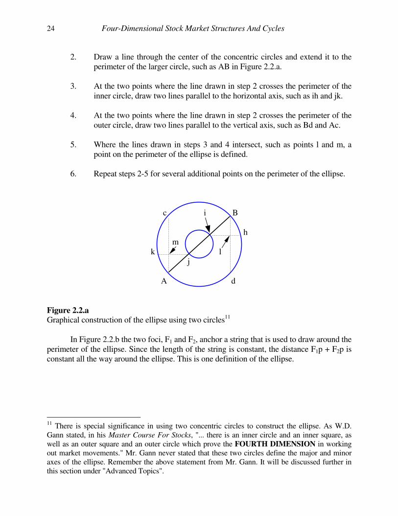
24 Four-Dimensional Stock Market Structures And Cycles
2. Draw a line through the center of the concentric circles and extend it to the
perimeter of the larger circle, such as AB in Figure 2.2.a. 3. At the two points where the line drawn in step 2 crosses the perimeter of the
inner circle, draw two lines parallel to the horizontal axis, such as ih and jk. 4. At the two points where the line drawn in step 2 crosses the perimeter of the
outer circle, draw two lines parallel to the vertical axis, such as Bd and Ac. 5. Where the lines drawn in steps 3 and 4 intersect, such as points l and m, a
point on the perimeter of the ellipse is defined. 6. Repeat steps 2-5 for several additional points on the perimeter of the ellipse.
c i B
h m k l j
A d
Figure 2.2.a
Graphical construction of the ellipse using two circles11 In Figure 2.2.b the two foci, F1 and F2, anchor a string that is used to draw around the perimeter of the ellipse. Since the length of the string is constant, the distance F1p + F2p is constant all the way around the ellipse. This is one definition of the ellipse.
11 There is special significance in using two concentric circles to construct the ellipse. As W.D. Gann stated, in his Master Course For Stocks, "... there is an inner circle and an inner square, as well as an outer square and an outer circle which prove the FOURTH DIMENSION in working out market movements." Mr. Gann never stated that these two circles define the major and minor axes of the ellipse. Remember the above statement from Mr. Gann. It will be discussed further in this section under "Advanced Topics".
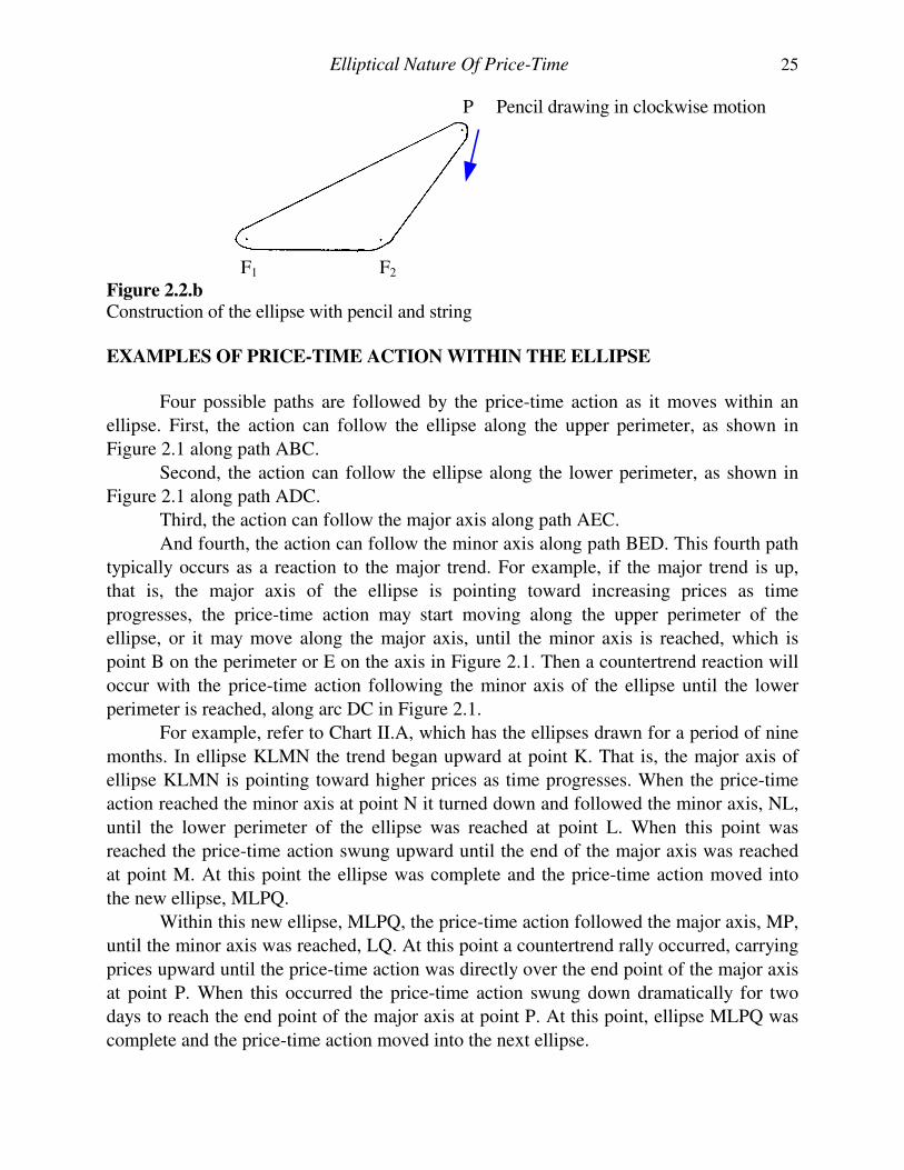
Elliptical Nature Of Price-Time 25
P Pencil drawing in clockwise motion
F1 F2
Figure 2.2.b Construction of the ellipse with pencil and string
EXAMPLES OF PRICE-TIME ACTION WITHIN THE ELLIPSE
Four possible paths are followed by the price-time action as it moves within an
ellipse. First, the action can follow the ellipse along the upper perimeter, as shown in
Figure 2.1 along path ABC.
Second, the action can follow the ellipse along the lower perimeter, as shown in
Figure 2.1 along path ADC.
Third, the action can follow the major axis along path AEC.
And fourth, the action can follow the minor axis along path BED. This fourth path
typically occurs as a reaction to the major trend. For example, if the major trend is up,
that is, the major axis of the ellipse is pointing toward increasing prices as time
progresses, the price-time action may start moving along the upper perimeter of the
ellipse, or it may move along the major axis, until the minor axis is reached, which is
point B on the perimeter or E on the axis in Figure 2.1. Then a countertrend reaction will
occur with the price-time action following the minor axis of the ellipse until the lower
perimeter is reached, along arc DC in Figure 2.1.
For example, refer to Chart II.A, which has the ellipses drawn for a period of nine
months. In ellipse KLMN the trend began upward at point K. That is, the major axis of
ellipse KLMN is pointing toward higher prices as time progresses. When the price-time
action reached the minor axis at point N it turned down and followed the minor axis, NL,
until the lower perimeter of the ellipse was reached at point L. When this point was
reached the price-time action swung upward until the end of the major axis was reached
at point M. At this point the ellipse was complete and the price-time action moved into
the new ellipse, MLPQ.
Within this new ellipse, MLPQ, the price-time action followed the major axis, MP,
until the minor axis was reached, LQ. At this point a countertrend rally occurred, carrying
prices upward until the price-time action was directly over the end point of the major axis
at point P. When this occurred the price-time action swung down dramatically for two
days to reach the end point of the major axis at point P. At this point, ellipse MLPQ was
complete and the price-time action moved into the next ellipse.
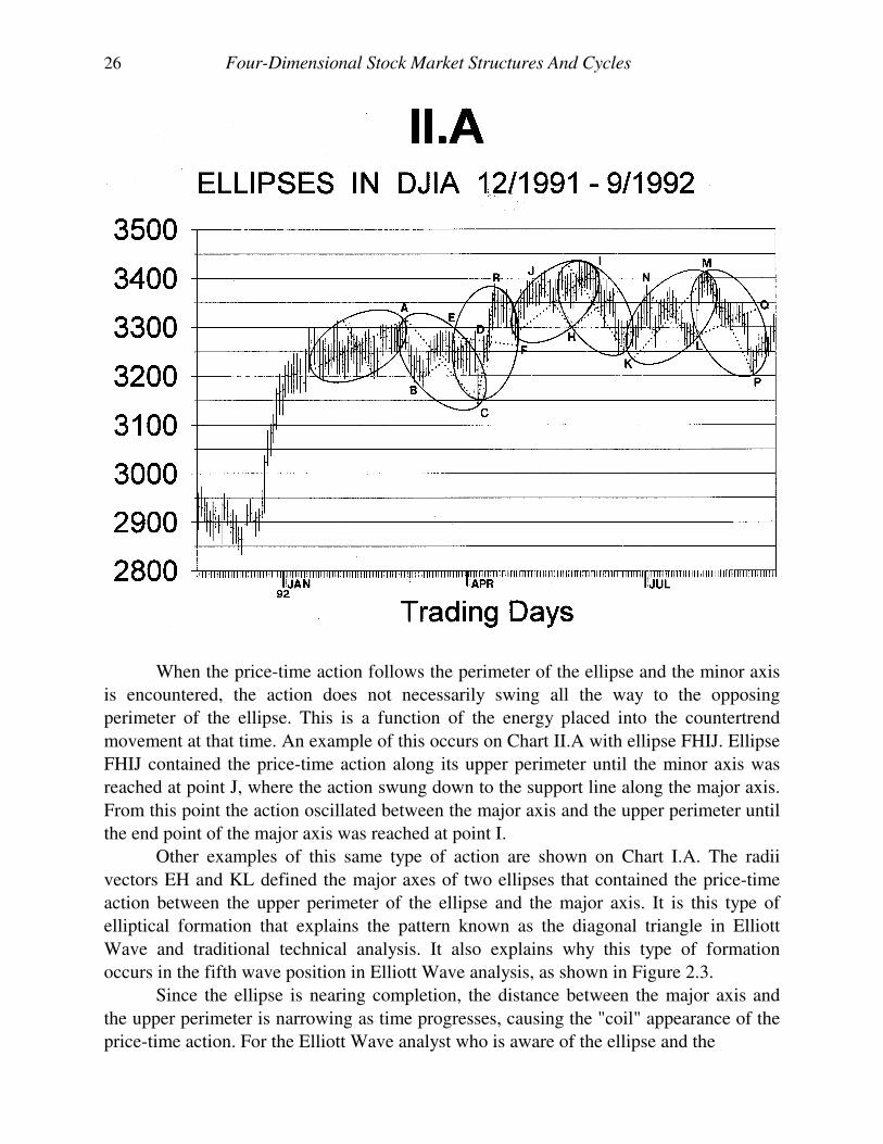
26 Four-Dimensional Stock Market Structures And Cycles
When the price-time action follows the perimeter of the ellipse and the minor axis
is encountered, the action does not necessarily swing all the way to the opposing
perimeter of the ellipse. This is a function of the energy placed into the countertrend
movement at that time. An example of this occurs on Chart II.A with ellipse FHIJ. Ellipse
FHIJ contained the price-time action along its upper perimeter until the minor axis was
reached at point J, where the action swung down to the support line along the major axis.
From this point the action oscillated between the major axis and the upper perimeter until
the end point of the major axis was reached at point I.
Other examples of this same type of action are shown on Chart I.A. The radii
vectors EH and KL defined the major axes of two ellipses that contained the price-time
action between the upper perimeter of the ellipse and the major axis. It is this type of
elliptical formation that explains the pattern known as the diagonal triangle in Elliott
Wave and traditional technical analysis. It also explains why this type of formation
occurs in the fifth wave position in Elliott Wave analysis, as shown in Figure 2.3.
Since the ellipse is nearing completion, the distance between the major axis and
the upper perimeter is narrowing as time progresses, causing the "coil" appearance of the
price-time action. For the Elliott Wave analyst who is aware of the ellipse and the
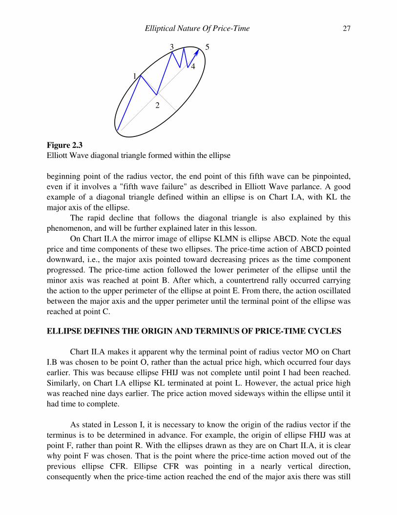
Elliptical Nature Of Price-Time 27
3 5
4
1
2
Figure 2.3
Elliott Wave diagonal triangle formed within the ellipse
beginning point of the radius vector, the end point of this fifth wave can be pinpointed,
even if it involves a "fifth wave failure" as described in Elliott Wave parlance. A good
example of a diagonal triangle defined within an ellipse is on Chart I.A, with KL the
major axis of the ellipse.
The rapid decline that follows the diagonal triangle is also explained by this
phenomenon, and will be further explained later in this lesson.
On Chart II.A the mirror image of ellipse KLMN is ellipse ABCD. Note the equal
price and time components of these two ellipses. The price-time action of ABCD pointed
downward, i.e., the major axis pointed toward decreasing prices as the time component
progressed. The price-time action followed the lower perimeter of the ellipse until the
minor axis was reached at point B. After which, a countertrend rally occurred carrying
the action to the upper perimeter of the ellipse at point E. From there, the action oscillated
between the major axis and the upper perimeter until the terminal point of the ellipse was
reached at point C.
ELLIPSE DEFINES THE ORIGIN AND TERMINUS OF PRICE-TIME CYCLES
Chart II.A makes it apparent why the terminal point of radius vector MO on Chart
I.B was chosen to be point O, rather than the actual price high, which occurred four days
earlier. This was because ellipse FHIJ was not complete until point I had been reached.
Similarly, on Chart I.A ellipse KL terminated at point L. However, the actual price high
was reached nine days earlier. The price action moved sideways within the ellipse until it
had time to complete.
As stated in Lesson I, it is necessary to know the origin of the radius vector if the
terminus is to be determined in advance. For example, the origin of ellipse FHIJ was at
point F, rather than point R. With the ellipses drawn as they are on Chart II.A, it is clear
why point F was chosen. That is the point where the price-time action moved out of the
previous ellipse CFR. Ellipse CFR was pointing in a nearly vertical direction,
consequently when the price-time action reached the end of the major axis there was still
28 Four-Dimensional Stock Market Structures And Cycles
considerable space left within ellipse CFR, specifically, the distance from point R to
point F. The action drifted along the outer perimeter of the ellipse until time had
progressed enough for it to move out of the ellipse. This was the origin of ellipse FHIJ.
MAJOR AXES OF MATED ELLIPSES FORM EQUILATERAL TRIANGLES
A very powerful, yet simple, technique that allows the analyst to fix in advance a specific point in price-time will now be explained. This technique is another of many provided in this course that were discovered by the author and are not available from any other source. This simple technique allows not only accurate price projects to be made, but even more importantly, identifies WHEN these price levels will be reached. The "Advanced Topics" section of Lesson I explained that price-time radii vectors formed the sides of equilateral triangles. Basic geometry identifies the inner angle of an equilateral triangle as 60 degrees. Also, Lesson I demonstrated that the length of the PTV is fixed. Therefore, given the angle and the length of the vector, the future point in price-time is fixed. For example, on Chart I.A when the location of radius vector AB had been fixed point C was fixed in price-time as well. This is because the angle from the AB axis is 60 degrees, and the length of the radius vector is constant, i.e., 236. This is graphically demonstrated in Figure 2.4, where three different orientations of an equilateral triangle are shown. The triangles shown in these three figures are the same, but are progressively rotated in a clockwise direction. In Figure 2.4.a the PTV, AB, that forms the first side of the equilateral triangle is nearly vertical causing its mated PTV, BC, to have very little price depreciation, since its direction is more parallel to the time axis. A slowly declining market consuming considerable time characterizes this orientation of mated ellipses. A good example in the DJIA of this type of configuration is shown on Chart II.B, where points F, G, H correspond with points A, B, C from Figure 2.4.a. Since FG was nearly vertical, its mated PTV, GH, moved sideways along the time axis resulting in very little price depreciation.
In Figure 2.4.b the first side of the equilateral triangle represented by PTV, DE,
angles more toward the time axis causing its mated PTV, EF, to point down more in price
that the one in Figure 2.4.a. A good example of this type of orientation is shown on Chart
II.B, where the points A, B, C correspond with points D, E, F in Figure 2.4.b. Notice that
the PTV, AB, was angled more toward the time axis than was FG. This means that the
PTV that was the mate of AB pointed down in price more than the PTV that was the mate
of FG, i.e., BC drops much more in price and consumes less time doing so than does GH.
In Figure 2.4.c, the PTV, GH, points nearly parallel to the time axis causing its
mated PTV, HI, to point nearly straight down in price. This type of market is very
dangerous for traders because the slow sideways movement along GH puts traders to
sleep and they lose their immediate attention to what is happening in the market.
However, when GH has run its course its mated PTV, HI, represents a dramatic decline in
prices in a very short time span. An example of this type of market configuration is
shown on Chart II.B, where DE angled more toward the time axis than did either FG or
AB. Notice that along DE almost all the price appreciation occurred
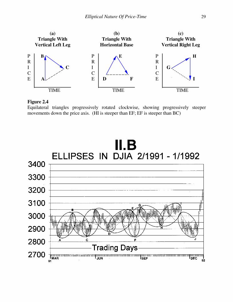
Elliptical Nature Of Price-Time 29
(a)
Triangle With
Vertical Left Leg
P B
R I C
C E A
TIME
(b)
Triangle With
Horizontal Base
P E
R I C E D F
TIME
(c)
Triangle With
Vertical Right Leg
P H
R I G
C E I
TIME
Figure 2.4
Equilateral triangles progressively rotated clockwise, showing progressively steeper movements down the price axis. (HI is steeper than EF; EF is steeper than BC)
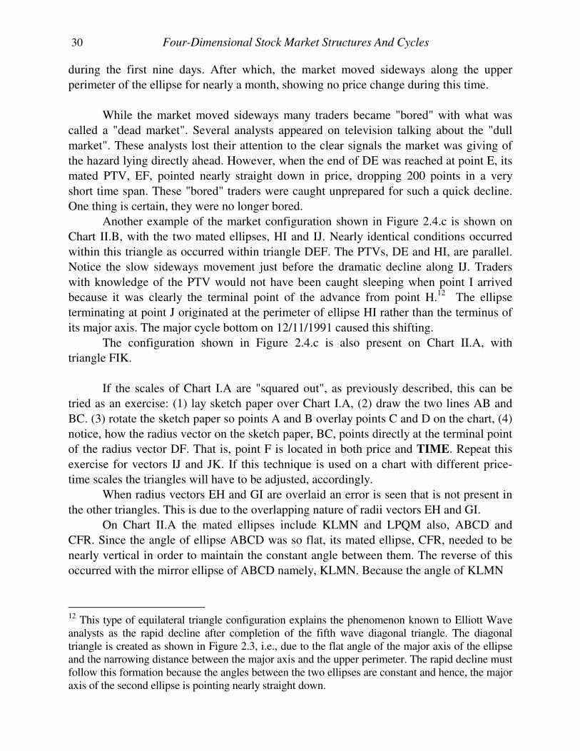
30 Four-Dimensional Stock Market Structures And Cycles
during the first nine days. After which, the market moved sideways along the upper
perimeter of the ellipse for nearly a month, showing no price change during this time.
While the market moved sideways many traders became "bored" with what was
called a "dead market". Several analysts appeared on television talking about the "dull
market". These analysts lost their attention to the clear signals the market was giving of
the hazard lying directly ahead. However, when the end of DE was reached at point E, its
mated PTV, EF, pointed nearly straight down in price, dropping 200 points in a very
short time span. These "bored" traders were caught unprepared for such a quick decline.
One thing is certain, they were no longer bored.
Another example of the market configuration shown in Figure 2.4.c is shown on
Chart II.B, with the two mated ellipses, HI and IJ. Nearly identical conditions occurred
within this triangle as occurred within triangle DEF. The PTVs, DE and HI, are parallel.
Notice the slow sideways movement just before the dramatic decline along IJ. Traders
with knowledge of the PTV would not have been caught sleeping when point I arrived
because it was clearly the terminal point of the advance from point H.12 The ellipse
terminating at point J originated at the perimeter of ellipse HI rather than the terminus of
its major axis. The major cycle bottom on 12/11/1991 caused this shifting.
The configuration shown in Figure 2.4.c is also present on Chart II.A, with
triangle FIK.
If the scales of Chart I.A are "squared out", as previously described, this can be
tried as an exercise: (1) lay sketch paper over Chart I.A, (2) draw the two lines AB and
BC. (3) rotate the sketch paper so points A and B overlay points C and D on the chart, (4)
notice, how the radius vector on the sketch paper, BC, points directly at the terminal point
of the radius vector DF. That is, point F is located in both price and TIME. Repeat this
exercise for vectors IJ and JK. If this technique is used on a chart with different price-
time scales the triangles will have to be adjusted, accordingly.
When radius vectors EH and GI are overlaid an error is seen that is not present in
the other triangles. This is due to the overlapping nature of radii vectors EH and GI.
On Chart II.A the mated ellipses include KLMN and LPQM also, ABCD and
CFR. Since the angle of ellipse ABCD was so flat, its mated ellipse, CFR, needed to be
nearly vertical in order to maintain the constant angle between them. The reverse of this
occurred with the mirror ellipse of ABCD namely, KLMN. Because the angle of KLMN
12 This type of equilateral triangle configuration explains the phenomenon known to Elliott Wave analysts as the rapid decline after completion of the fifth wave diagonal triangle. The diagonal triangle is created as shown in Figure 2.3, i.e., due to the flat angle of the major axis of the ellipse and the narrowing distance between the major axis and the upper perimeter. The rapid decline must follow this formation because the angles between the two ellipses are constant and hence, the major axis of the second ellipse is pointing nearly straight down.
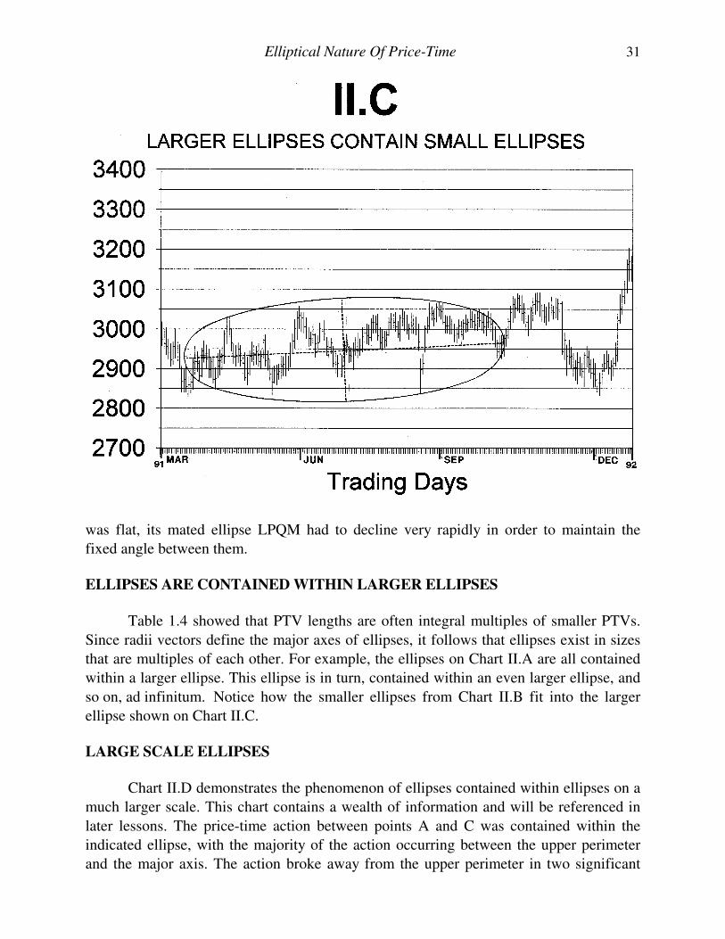
Elliptical Nature Of Price-Time 31
was flat, its mated ellipse LPQM had to decline very rapidly in order to maintain the
fixed angle between them.
ELLIPSES ARE CONTAINED WITHIN LARGER ELLIPSES
Table 1.4 showed that PTV lengths are often integral multiples of smaller PTVs.
Since radii vectors define the major axes of ellipses, it follows that ellipses exist in sizes
that are multiples of each other. For example, the ellipses on Chart II.A are all contained
within a larger ellipse. This ellipse is in turn, contained within an even larger ellipse, and
so on, ad infinitum. Notice how the smaller ellipses from Chart II.B fit into the larger
ellipse shown on Chart II.C.
LARGE SCALE ELLIPSES
Chart II.D demonstrates the phenomenon of ellipses contained within ellipses on a
much larger scale. This chart contains a wealth of information and will be referenced in
later lessons. The price-time action between points A and C was contained within the
indicated ellipse, with the majority of the action occurring between the upper perimeter
and the major axis. The action broke away from the upper perimeter in two significant
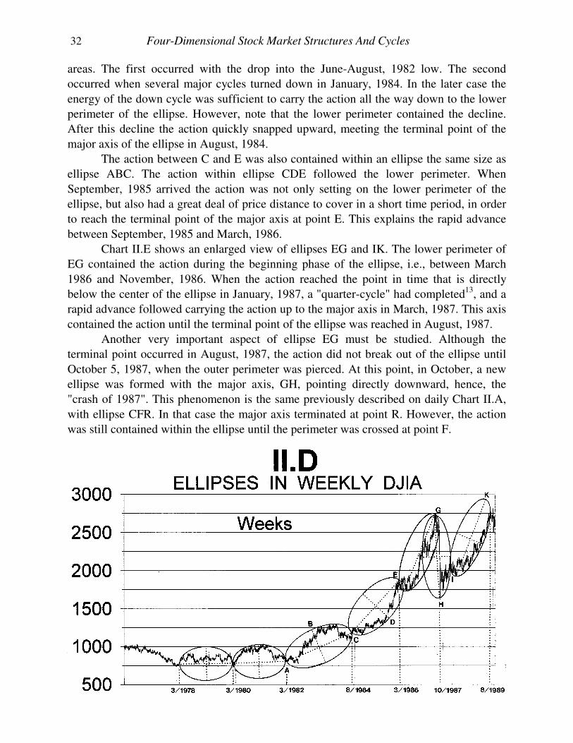
32 Four-Dimensional Stock Market Structures And Cycles
areas. The first occurred with the drop into the June-August, 1982 low. The second
occurred when several major cycles turned down in January, 1984. In the later case the
energy of the down cycle was sufficient to carry the action all the way down to the lower
perimeter of the ellipse. However, note that the lower perimeter contained the decline.
After this decline the action quickly snapped upward, meeting the terminal point of the
major axis of the ellipse in August, 1984.
The action between C and E was also contained within an ellipse the same size as
ellipse ABC. The action within ellipse CDE followed the lower perimeter. When
September, 1985 arrived the action was not only setting on the lower perimeter of the
ellipse, but also had a great deal of price distance to cover in a short time period, in order
to reach the terminal point of the major axis at point E. This explains the rapid advance
between September, 1985 and March, 1986.
Chart II.E shows an enlarged view of ellipses EG and IK. The lower perimeter of
EG contained the action during the beginning phase of the ellipse, i.e., between March
1986 and November, 1986. When the action reached the point in time that is directly
below the center of the ellipse in January, 1987, a "quarter-cycle" had completed13, and a
rapid advance followed carrying the action up to the major axis in March, 1987. This axis
contained the action until the terminal point of the ellipse was reached in August, 1987.
Another very important aspect of ellipse EG must be studied. Although the
terminal point occurred in August, 1987, the action did not break out of the ellipse until
October 5, 1987, when the outer perimeter was pierced. At this point, in October, a new
ellipse was formed with the major axis, GH, pointing directly downward, hence, the
"crash of 1987". This phenomenon is the same previously described on daily Chart II.A,
with ellipse CFR. In that case the major axis terminated at point R. However, the action
was still contained within the ellipse until the perimeter was crossed at point F.
13 The "quarter-cycle" describes the action referred to by several technical analysts as, "base building before the advance".
Elliptical Nature Of Price-Time 33
Ellipse GH is much simpler to describe. Simply stated, it pointed down! Within
this ellipse the gap occurred when the action reached the center point of the ellipse along
the major axis.
The same phenomenon occurred between ellipses GH and IK that occurred
between ellipses EG and GH. Namely, the price action hit its low in October, 1987, when
the terminal point of the major axis had been reached. However, the new ellipse, IK, did
not begin until March, 1988 at point I, where the action pierced the perimeter of the
previous ellipse, GH.
Ellipse IK was similar in form to ellipse CD. It followed the lower perimeter of the
ellipse until the action moved directly below the center point of the ellipse. At this point
in November, 1988, the "quarter-cycle" was complete and the action moved dramatically
upward to reach the terminal point of the major axis at point K. The action between
March, 1988 and November, 1988 defined the "base before the advance", as described
above.
The ellipses contained on Charts II.D and II.E are multiples of the much smaller
ellipses, shown on the daily charts II.A and II.B. Methods for determining these ratios
will be presented in later lessons.
ADVANCED TOPICS
It was previously noted that there is special significance to using two circles to
form the ellipse. It was also noted in Lesson I that traditional price-time charts are limited
in the sense that they are two-dimensional representations of a multi-dimensional
phenomenon. The inner circle of the ellipse is actually at a higher dimension than the
outer circle.14 To visualize this, imagine a conic section with circles stacked on top of
each other, each with a diameter smaller than the previous circle until the vortex is
reached. The ellipse is formed from two such circles with the price-time action actually
moving out of the limits of the two-dimensional representation of the price-time chart.
CONCLUSION
At this point in the course the reader should be able to:
- Construct an ellipse from two concentric circles.
- Identify an ellipse on a price-time chart.
- Use a PTV, as identified in Lesson I, as the major or minor axis of the
ellipse and construct the ellipse.
- Recognize equilateral triangles on price-time charts and use them to
project the terminal point of a PTV.
- Identify the 1/2 and 1/4 cycles of the ellipse.
14 This is what W.D. Gann meant when he stated, "... there is an inner circle and an inner square, as well as an outer square and an outer circle which prove the fourth-dimension in working out market movements."
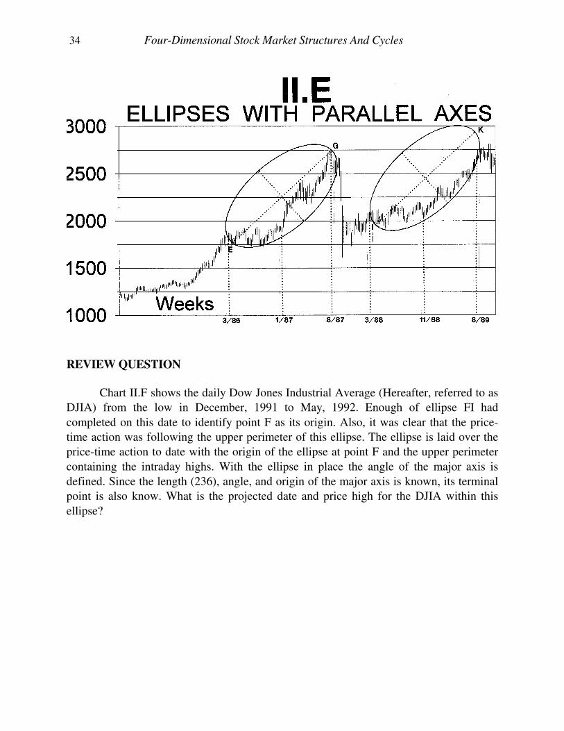
34 Four-Dimensional Stock Market Structures And Cycles
REVIEW QUESTION
Chart II.F shows the daily Dow Jones Industrial Average (Hereafter, referred to as
DJIA) from the low in December, 1991 to May, 1992. Enough of ellipse FI had
completed on this date to identify point F as its origin. Also, it was clear that the price-
time action was following the upper perimeter of this ellipse. The ellipse is laid over the
price-time action to date with the origin of the ellipse at point F and the upper perimeter
containing the intraday highs. With the ellipse in place the angle of the major axis is
defined. Since the length (236), angle, and origin of the major axis is known, its terminal
point is also know. What is the projected date and price high for the DJIA within this
ellipse?
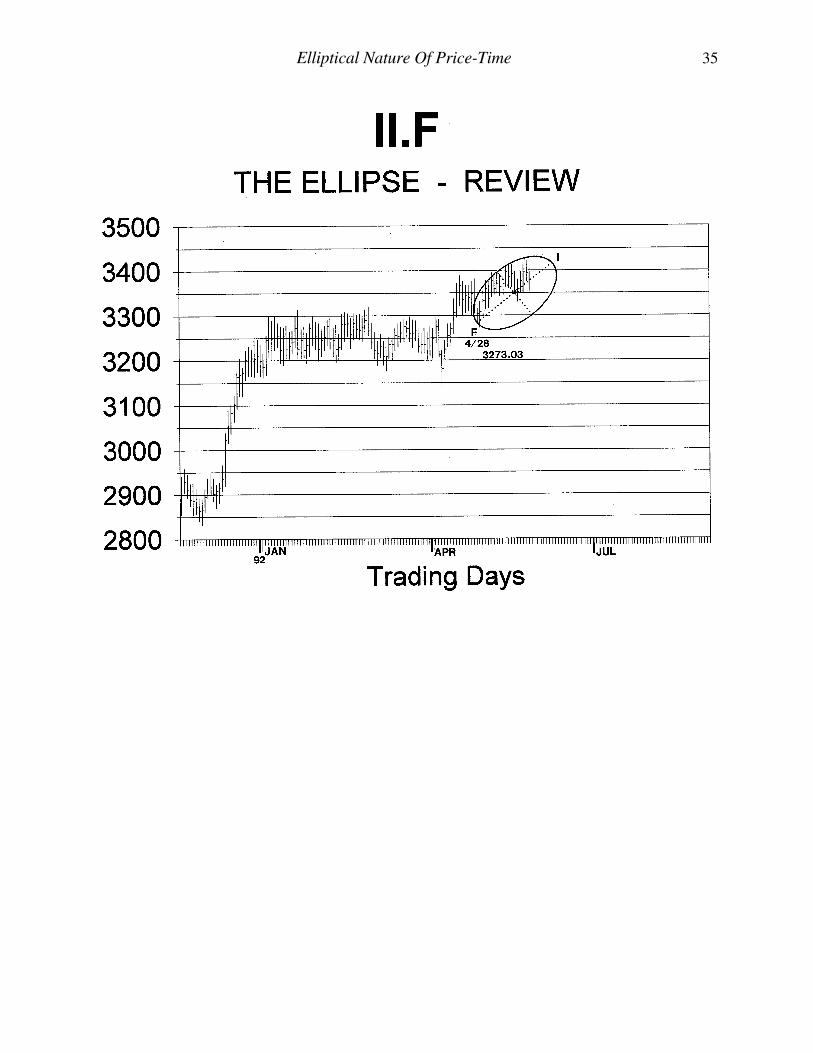
Elliptical Nature Of Price-Time 35
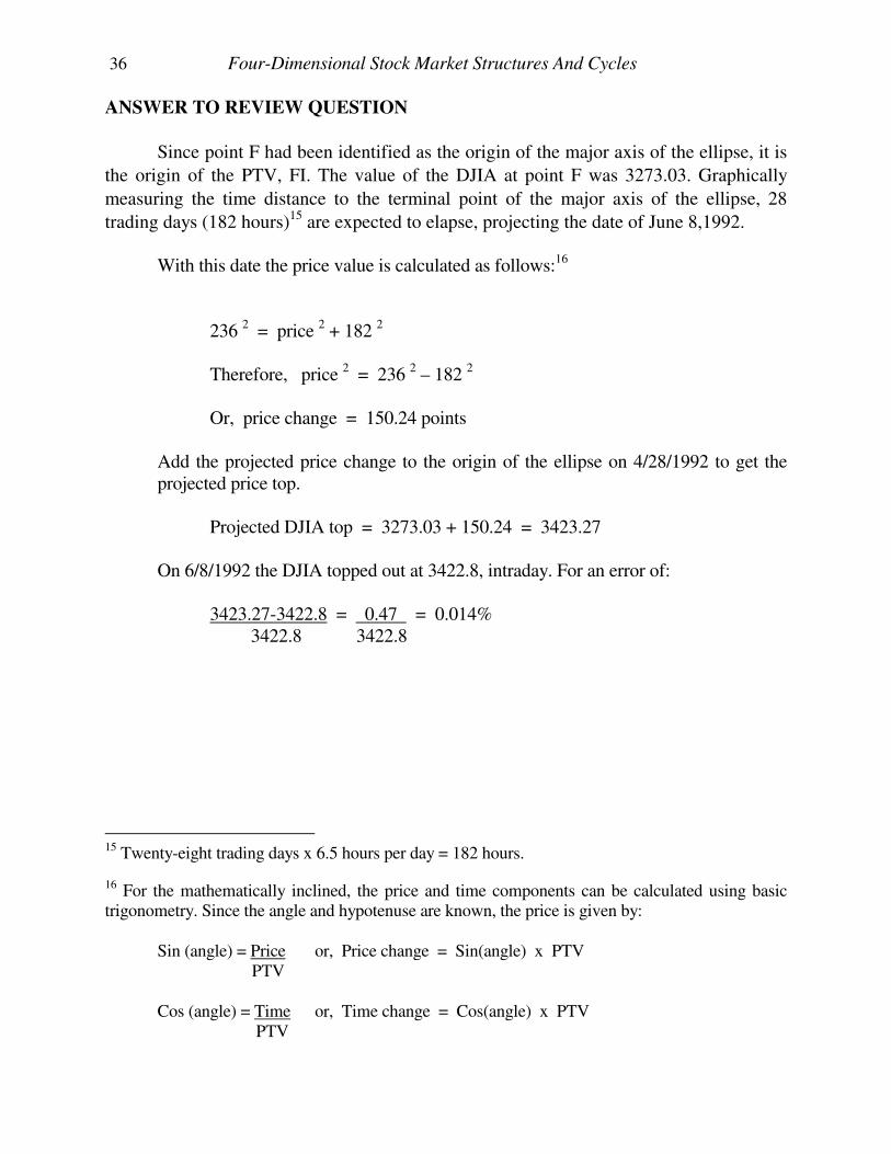
36 Four-Dimensional Stock Market Structures And Cycles
ANSWER TO REVIEW QUESTION
Since point F had been identified as the origin of the major axis of the ellipse, it is
the origin of the PTV, FI. The value of the DJIA at point F was 3273.03. Graphically
measuring the time distance to the terminal point of the major axis of the ellipse, 28
trading days (182 hours)15 are expected to elapse, projecting the date of June 8,1992. With this date the price value is calculated as follows:16
236 2 = price 2 + 182 2 Therefore, price 2 = 236 2 – 182 2 Or, price change = 150.24 points
Add the projected price change to the origin of the ellipse on 4/28/1992 to get the projected price top.
Projected DJIA top = 3273.03 + 150.24 = 3423.27 On 6/8/1992 the DJIA topped out at 3422.8, intraday. For an error of: 3423.27-3422.8 = 0.47 = 0.014% 3422.8 3422.8
15 Twenty-eight trading days x 6.5 hours per day = 182 hours.
16 For the mathematically inclined, the price and time components can be calculated using basic trigonometry. Since the angle and hypotenuse are known, the price is given by: Sin (angle) = Price or, Price change = Sin(angle) x PTV PTV Cos (angle) = Time or, Time change = Cos(angle) x PTV PTV
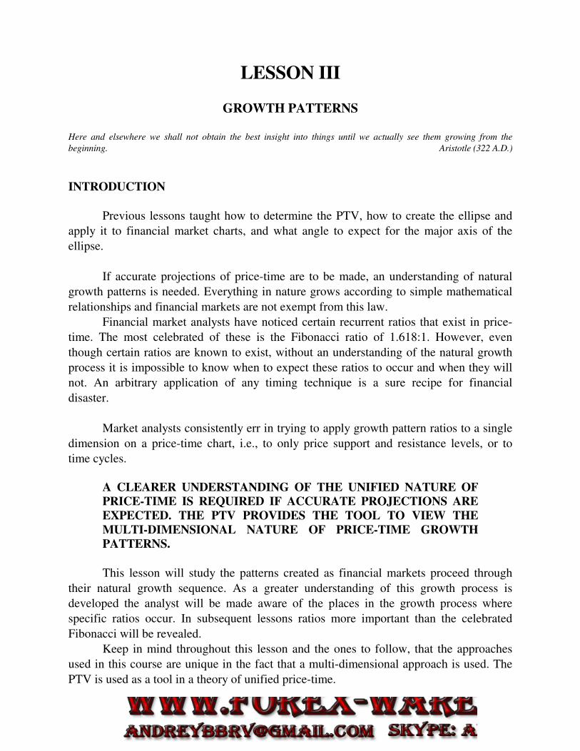
LESSON III
GROWTH PATTERNS
Here and elsewhere we shall not obtain the best insight into things until we actually see them growing from the
beginning. Aristotle (322 A.D.)
INTRODUCTION
Previous lessons taught how to determine the PTV, how to create the ellipse and
apply it to financial market charts, and what angle to expect for the major axis of the
ellipse.
If accurate projections of price-time are to be made, an understanding of natural
growth patterns is needed. Everything in nature grows according to simple mathematical
relationships and financial markets are not exempt from this law.
Financial market analysts have noticed certain recurrent ratios that exist in price-
time. The most celebrated of these is the Fibonacci ratio of 1.618:1. However, even
though certain ratios are known to exist, without an understanding of the natural growth
process it is impossible to know when to expect these ratios to occur and when they will
not. An arbitrary application of any timing technique is a sure recipe for financial
disaster.
Market analysts consistently err in trying to apply growth pattern ratios to a single
dimension on a price-time chart, i.e., to only price support and resistance levels, or to
time cycles.
A CLEARER UNDERSTANDING OF THE UNIFIED NATURE OF
PRICE-TIME IS REQUIRED IF ACCURATE PROJECTIONS ARE
EXPECTED. THE PTV PROVIDES THE TOOL TO VIEW THE
MULTI-DIMENSIONAL NATURE OF PRICE-TIME GROWTH
PATTERNS.
This lesson will study the patterns created as financial markets proceed through
their natural growth sequence. As a greater understanding of this growth process is
developed the analyst will be made aware of the places in the growth process where
specific ratios occur. In subsequent lessons ratios more important than the celebrated
Fibonacci will be revealed.
Keep in mind throughout this lesson and the ones to follow, that the approaches
used in this course are unique in the fact that a multi-dimensional approach is used. The
PTV is used as a tool in a theory of unified price-time.
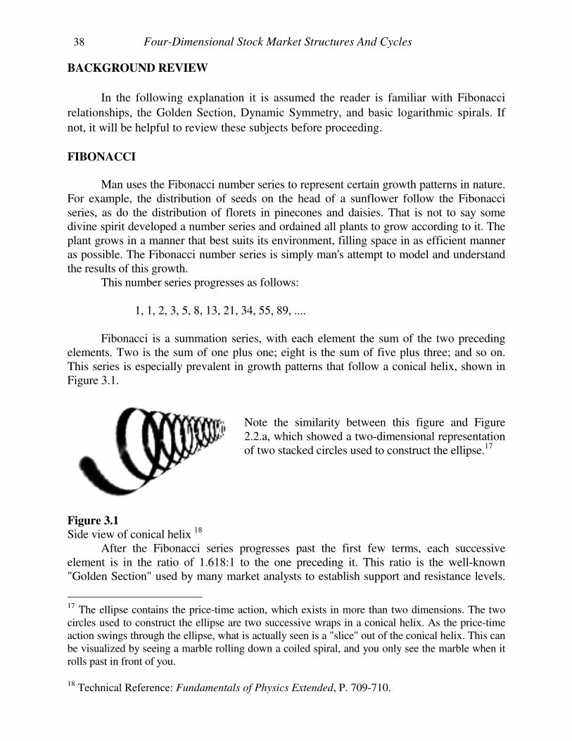
38 Four-Dimensional Stock Market Structures And Cycles
BACKGROUND REVIEW
In the following explanation it is assumed the reader is familiar with Fibonacci
relationships, the Golden Section, Dynamic Symmetry, and basic logarithmic spirals. If
not, it will be helpful to review these subjects before proceeding.
FIBONACCI
Man uses the Fibonacci number series to represent certain growth patterns in nature. For example, the distribution of seeds on the head of a sunflower follow the Fibonacci series, as do the distribution of florets in pinecones and daisies. That is not to say some divine spirit developed a number series and ordained all plants to grow according to it. The plant grows in a manner that best suits its environment, filling space in as efficient manner as possible. The Fibonacci number series is simply man's attempt to model and understand the results of this growth. This number series progresses as follows: 1, 1, 2, 3, 5, 8, 13, 21, 34, 55, 89, .... Fibonacci is a summation series, with each element the sum of the two preceding elements. Two is the sum of one plus one; eight is the sum of five plus three; and so on. This series is especially prevalent in growth patterns that follow a conical helix, shown in Figure 3.1.
Note the similarity between this figure and Figure 2.2.a, which showed a two-dimensional representation of two stacked circles used to construct the ellipse.17
Figure 3.1
Side view of conical helix 18 After the Fibonacci series progresses past the first few terms, each successive element is in the ratio of 1.618:1 to the one preceding it. This ratio is the well-known "Golden Section" used by many market analysts to establish support and resistance levels.
17 The ellipse contains the price-time action, which exists in more than two dimensions. The two circles used to construct the ellipse are two successive wraps in a conical helix. As the price-time action swings through the ellipse, what is actually seen is a "slice" out of the conical helix. This can be visualized by seeing a marble rolling down a coiled spiral, and you only see the marble when it rolls past in front of you. 18 Technical Reference: Fundamentals of Physics Extended, P. 709-710.
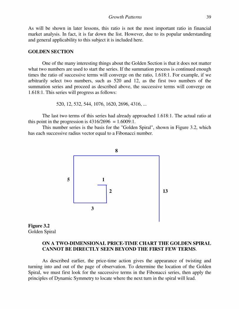
Growth Patterns 39
As will be shown in later lessons, this ratio is not the most important ratio in financial market analysis. In fact, it is far down the list. However, due to its popular understanding and general applicability to this subject it is included here. GOLDEN SECTION
One of the many interesting things about the Golden Section is that it does not matter what two numbers are used to start the series. If the summation process is continued enough times the ratio of successive terms will converge on the ratio, 1.618:1. For example, if we arbitrarily select two numbers, such as 520 and 12, as the first two numbers of the summation series and proceed as described above, the successive terms will converge on 1.618:1. This series will progress as follows: 520, 12, 532, 544, 1076, 1620, 2696, 4316, ... The last two terms of this series had already approached 1.618:1. The actual ratio at this point in the progression is 4316/2696 = 1.6009:1. This number series is the basis for the "Golden Spiral", shown in Figure 3.2, which has each successive radius vector equal to a Fibonacci number.
8 5 1 2 13 3 Figure 3.2 Golden Spiral
ON A TWO-DIMENSIONAL PRICE-TIME CHART THE GOLDEN SPIRAL CANNOT BE DIRECTLY SEEN BEYOND THE FIRST FEW TERMS.
As described earlier, the price-time action gives the appearance of twisting and turning into and out of the page of observation. To determine the location of the Golden Spiral, we must first look for the successive terms in the Fibonacci series, then apply the principles of Dynamic Symmetry to locate where the next turn in the spiral will lead.
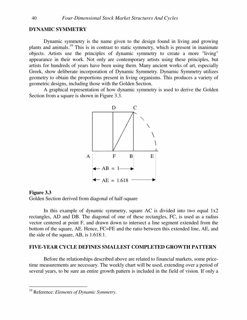
40 Four-Dimensional Stock Market Structures And Cycles
DYNAMIC SYMMETRY
Dynamic symmetry is the name given to the design found in living and growing plants and animals.19 This is in contrast to static symmetry, which is present in inanimate objects. Artists use the principles of dynamic symmetry to create a more "living" appearance in their work. Not only are contemporary artists using these principles, but artists for hundreds of years have been using them. Many ancient works of art, especially Greek, show deliberate incorporation of Dynamic Symmetry. Dynamic Symmetry utilizes geometry to obtain the proportions present in living organisms. This produces a variety of geometric designs, including those with the Golden Section. A graphical representation of how dynamic symmetry is used to derive the Golden Section from a square is shown in Figure 3.3.
D C
A F B E AB = 1
AE = 1.618 Figure 3.3 Golden Section derived from diagonal of half-square In this example of dynamic symmetry, square AC is divided into two equal 1x2 rectangles, AD and DB. The diagonal of one of these rectangles, FC, is used as a radius vector centered at point F, and drawn down to intersect a line segment extended from the bottom of the square, AE. Hence, FC=FE and the ratio between this extended line, AE, and the side of the square, AB, is 1.618:1.
FIVE-YEAR CYCLE DEFINES SMALLEST COMPLETED GROWTH PATTERN
Before the relationships described above are related to financial markets, some price-time measurements are necessary. The weekly chart will be used, extending over a period of several years, to be sure an entire growth pattern is included in the field of vision. If only a
19 Reference: Elements of Dynamic Symmetry.
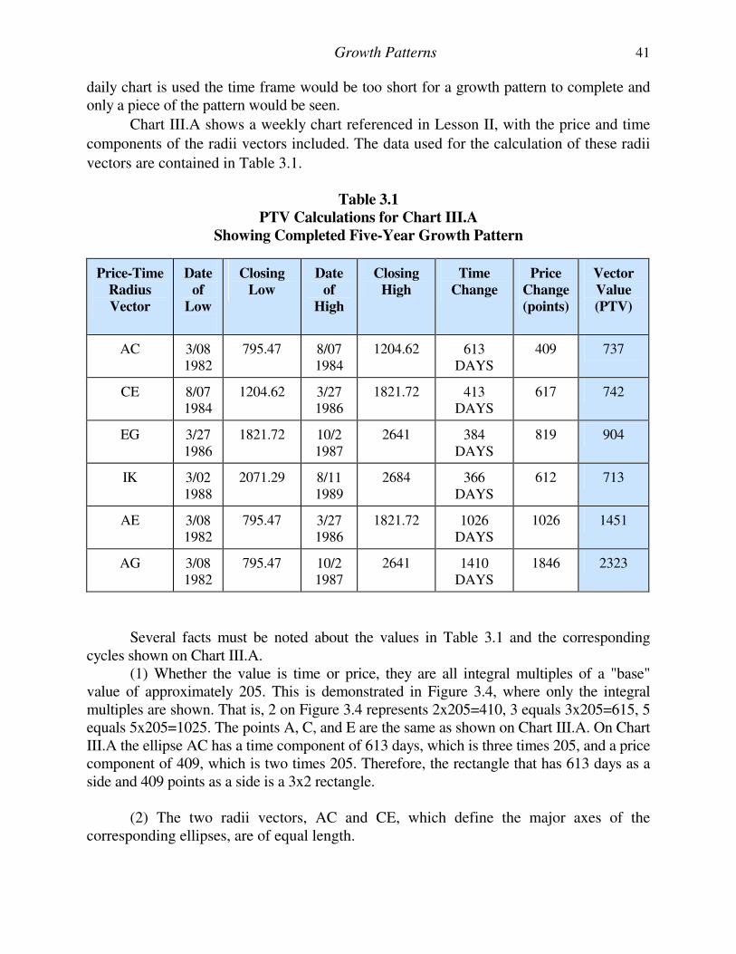
Growth Patterns 41
daily chart is used the time frame would be too short for a growth pattern to complete and only a piece of the pattern would be seen.
Chart III.A shows a weekly chart referenced in Lesson II, with the price and time
components of the radii vectors included. The data used for the calculation of these radii
vectors are contained in Table 3.1.
Table 3.1
PTV Calculations for Chart III.A
Showing Completed Five-Year Growth Pattern
Price-Time
Radius
Vector
Date
of
Low
Closing
Low
Date
of
High
Closing
High
Time
Change
Price
Change
(points)
Vector
Value
(PTV)
AC 3/08 1982
795.47 8/07 1984
1204.62 613 DAYS
409 737
CE 8/07 1984
1204.62 3/27 1986
1821.72 413 DAYS
617 742
EG 3/27 1986
1821.72 10/2 1987
2641 384 DAYS
819 904
IK 3/02 1988
2071.29 8/11 1989
2684 366 DAYS
612 713
AE 3/08 1982
795.47 3/27 1986
1821.72 1026 DAYS
1026 1451
AG 3/08 1982
795.47 10/2 1987
2641 1410 DAYS
1846 2323
Several facts must be noted about the values in Table 3.1 and the corresponding cycles shown on Chart III.A. (1) Whether the value is time or price, they are all integral multiples of a "base" value of approximately 205. This is demonstrated in Figure 3.4, where only the integral multiples are shown. That is, 2 on Figure 3.4 represents 2x205=410, 3 equals 3x205=615, 5 equals 5x205=1025. The points A, C, and E are the same as shown on Chart III.A. On Chart III.A the ellipse AC has a time component of 613 days, which is three times 205, and a price component of 409, which is two times 205. Therefore, the rectangle that has 613 days as a side and 409 points as a side is a 3x2 rectangle.
(2) The two radii vectors, AC and CE, which define the major axes of the corresponding ellipses, are of equal length.
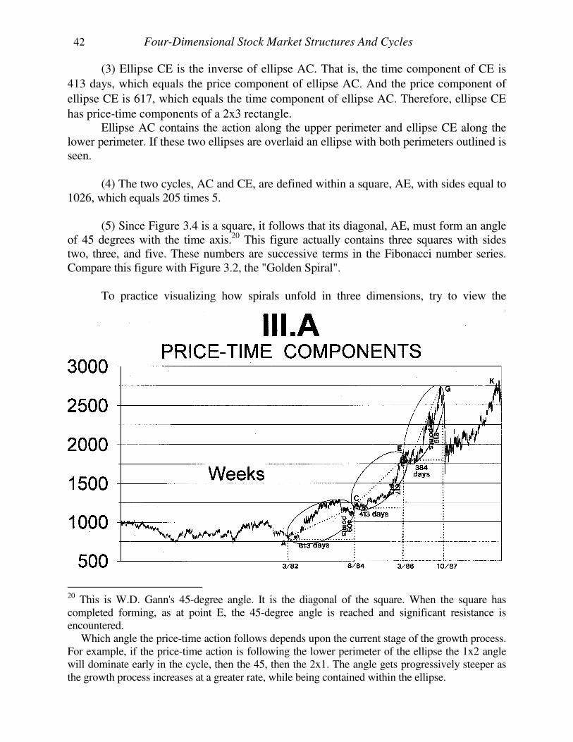
42 Four-Dimensional Stock Market Structures And Cycles
(3) Ellipse CE is the inverse of ellipse AC. That is, the time component of CE is
413 days, which equals the price component of ellipse AC. And the price component of
ellipse CE is 617, which equals the time component of ellipse AC. Therefore, ellipse CE
has price-time components of a 2x3 rectangle. Ellipse AC contains the action along the upper perimeter and ellipse CE along the lower perimeter. If these two ellipses are overlaid an ellipse with both perimeters outlined is seen. (4) The two cycles, AC and CE, are defined within a square, AE, with sides equal to 1026, which equals 205 times 5. (5) Since Figure 3.4 is a square, it follows that its diagonal, AE, must form an angle of 45 degrees with the time axis.20 This figure actually contains three squares with sides two, three, and five. These numbers are successive terms in the Fibonacci number series. Compare this figure with Figure 3.2, the "Golden Spiral". To practice visualizing how spirals unfold in three dimensions, try to view the twisting that would be required to place the 3x2 rectangle of ellipse AC over the 2x3 rectangle of ellipse CE.
20 This is W.D. Gann's 45-degree angle. It is the diagonal of the square. When the square has completed forming, as at point E, the 45-degree angle is reached and significant resistance is encountered. Which angle the price-time action follows depends upon the current stage of the growth process. For example, if the price-time action is following the lower perimeter of the ellipse the 1x2 angle will dominate early in the cycle, then the 45, then the 2x1. The angle gets progressively steeper as the growth process increases at a greater rate, while being contained within the ellipse.
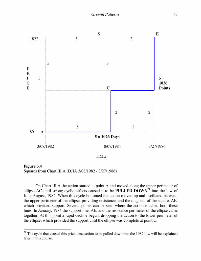
Growth Patterns 43
5 E 1822 3 2 3 3 P R I 5 5 =
C 1026 E C Points 2 2
3 2 804 A
5 = 1026 Days
3/08/1982 8/07/1984 3/27/1986
TIME
Figure 3.4 Squares from Chart III.A (DJIA 3/08/1982 - 3/27/1986) On Chart III.A the action started at point A and moved along the upper perimeter of ellipse AC until strong cyclic effects caused it to be PULLED DOWN
21 into the low of June-August, 1982. When this cycle bottomed the action moved up and oscillated between the upper perimeter of the ellipse, providing resistance, and the diagonal of the square, AE, which provided support. Several points can be seen where the action touched both these lines. In January, 1984 the support line, AE, and the resistance perimeter of the ellipse came together. At this point a rapid decline began, dropping the action to the lower perimeter of the ellipse, which provided the support until the ellipse was complete at point C.
21 The cycle that caused this price-time action to be pulled down into the 1982 low will be explained later in this course.
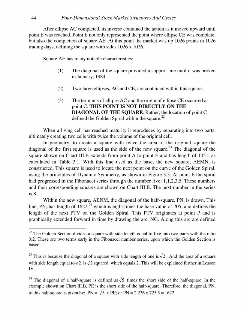
44 Four-Dimensional Stock Market Structures And Cycles
After ellipse AC completed, its inverse contained the action as it moved upward until point E was reached. Point E not only represented the point where ellipse CE was complete, but also the completion of square AE. At this point the market was up 1026 points in 1026 trading days, defining the square with sides 1026 x 1026. Square AE has many notable characteristics:
(1) The diagonal of the square provided a support line until it was broken in January, 1984.
(2) Two large ellipses, AC and CE, are contained within this square. (3) The terminus of ellipse AC and the origin of ellipse CE occurred at
point C. THIS POINT IS NOT DIRECTLY ON THE
DIAGONAL OF THE SQUARE. Rather, the location of point C defined the Golden Spiral within the square.22
When a living cell has reached maturity it reproduces by separating into two parts, ultimately creating two cells with twice the volume of the original cell.
In geometry, to create a square with twice the area of the original square the
diagonal of the first square is used as the side of the new square.23 The diagonal of the
square shown on Chart III.B extends from point A to point E and has length of 1451, as
calculated in Table 3.1. With this line used as the base, the new square, AEMN, is
constructed. This square is used to locate the next point on the curve of the Golden Spiral,
using the principles of Dynamic Symmetry, as shown in Figure 3.3. At point E the spiral
had progressed in the Fibonacci series through the number five: 1,1,2,3,5. These numbers
and their corresponding squares are shown on Chart III.B. The next number in the series
is 8.
Within the new square, AENM, the diagonal of the half-square, PN, is drawn. This
line, PN, has length of 1622,24 which is eight times the base value of 205, and defines the
length of the next PTV on the Golden Spiral. This PTV originates at point P and is
graphically extended forward in time by drawing the arc, NG. Along this arc are defined
22 The Golden Section divides a square with side length equal to five into two parts with the ratio 3:2. These are two terms early in the Fibonacci number series, upon which the Golden Section is based.
23 This is because the diagonal of a square with side length of one is 2 . And the area of a square
with side length equal to 2 is 2 squared, which equals 2. This will be explained further in Lesson IV.
24 The diagonal of a half-square is defined as 5 times the short side of the half-square. In the
example shown on Chart III.B, PE is the short side of the half-square. Therefore, the diagonal, PN,
to this half-square is given by; PN = 5 x PE; or PN = 2.236 x 725.5 = 1622.
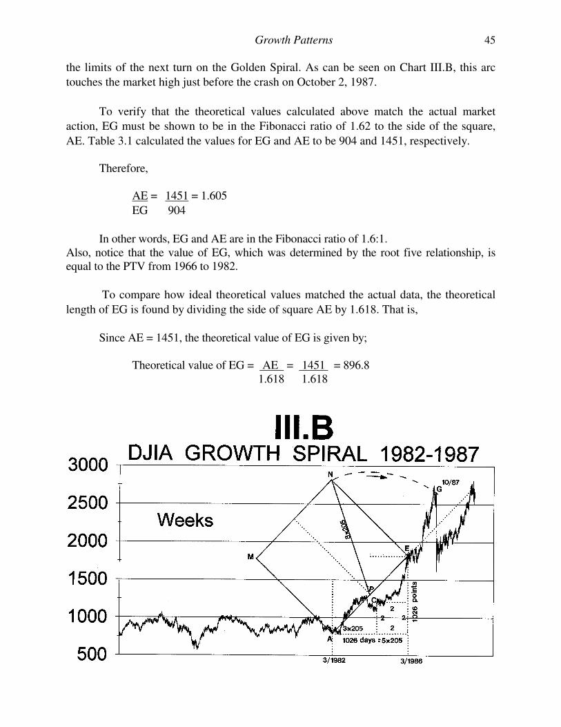
Growth Patterns 45
the limits of the next turn on the Golden Spiral. As can be seen on Chart III.B, this arc
touches the market high just before the crash on October 2, 1987.
To verify that the theoretical values calculated above match the actual market
action, EG must be shown to be in the Fibonacci ratio of 1.62 to the side of the square,
AE. Table 3.1 calculated the values for EG and AE to be 904 and 1451, respectively. Therefore,
AE = 1451 = 1.605
EG 904
In other words, EG and AE are in the Fibonacci ratio of 1.6:1. Also, notice that the value of EG, which was determined by the root five relationship, is equal to the PTV from 1966 to 1982.
To compare how ideal theoretical values matched the actual data, the theoretical
length of EG is found by dividing the side of square AE by 1.618. That is,
Since AE = 1451, the theoretical value of EG is given by; Theoretical value of EG = AE = 1451 = 896.8 1.618 1.618
46 Four-Dimensional Stock Market Structures And Cycles
The actual value of EG was 904, producing an error of, 904-896.8 = 0.80% error 896.8 Additional proof that the techniques of dynamic symmetry defined above identify the Golden Section within the five-year growth pattern on Chart III.B is obtained by verifying the PHI ratio between the PTVs AG and AE. AG = 2323 = 1.6 AE 1451
ADVANCED TOPICS
The reason dynamic symmetry is an invaluable tool in determining the final turn on the spiral of the completed five-year growth cycle is that the final PTV, EG, actually turned out of the page of observation. The dimensional distortions caused by two-dimensional charts create the appearance that the action is coming toward the observer as he views the chart.
LESSON IV
PRICE-TIME RATIOS
MORE IMPORTANT THAN FIBONACCI Mathematics ... reveals the orderliness of the ratios according to which the universe is constructed and the proportion
that binds things together in the cosmos.
Proclus Diadochus (485 A.D.) ...Commentary on the First Book of Euclid's Elements
INTRODUCTION
While the Fibonacci ratio (PHI=1.618) has gained recent popularity as a tool for financial market analysis, it is NOT the most valuable. There are several ratios that produce better results in timing financial markets if they are approached from the four-dimensional perspective. Without such a perspective the realities presented in this lesson and the lessons to follow remain unseen. The PTV provides the tool for a four-dimensional approach. The ratios presented in this lesson are produced as markets unfold in their characteristic geometric patterns.25 The only limitation in the time scale to which these ratios can be applied is the availability of reliable data. Financial markets continue to grow from their date of inception until their termination. If a financial market has been in existence for seven hundred years, (like the world-wide wheat market), PTV ratios can be calculated and applied to the geometric growth pattern for that time frame. In fact, the ratios presented in this lesson are present on price-time charts with time scales ranging from minutes to centuries.
A RATIO MUCH MORE IMPORTANT THAN FIBONACCI The square root of two, 1.414, is MUCH MORE IMPORTANT in financial market analysis than Fibonacci. The square root of two relates the diagonal of a square to its side, as in Figure 4.1. The square root of two ratio has many interesting properties, some common with Fibonacci. For example, if one is subtracted from the square root of two the result is 0.414.
2 - 1 = 0.414
If this value of 0.414 is divided into one, the result is one plus the square root of
two.
25 A more detailed explanation of financial market geometry is provided in Lesson V, GEOMETRIC STRUCTURES.
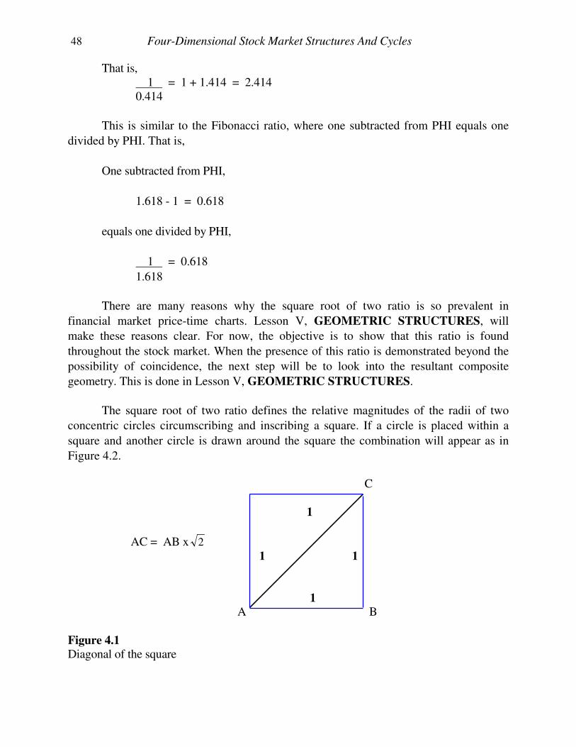
48 Four-Dimensional Stock Market Structures And Cycles
That is, 1 = 1 + 1.414 = 2.414 0.414
This is similar to the Fibonacci ratio, where one subtracted from PHI equals one
divided by PHI. That is,
One subtracted from PHI,
1.618 - 1 = 0.618
equals one divided by PHI,
1 = 0.618
1.618
There are many reasons why the square root of two ratio is so prevalent in
financial market price-time charts. Lesson V, GEOMETRIC STRUCTURES, will
make these reasons clear. For now, the objective is to show that this ratio is found
throughout the stock market. When the presence of this ratio is demonstrated beyond the
possibility of coincidence, the next step will be to look into the resultant composite
geometry. This is done in Lesson V, GEOMETRIC STRUCTURES.
The square root of two ratio defines the relative magnitudes of the radii of two
concentric circles circumscribing and inscribing a square. If a circle is placed within a
square and another circle is drawn around the square the combination will appear as in
Figure 4.2.
C 1
AC = AB x 2 1 1 1 A B
Figure 4.1
Diagonal of the square
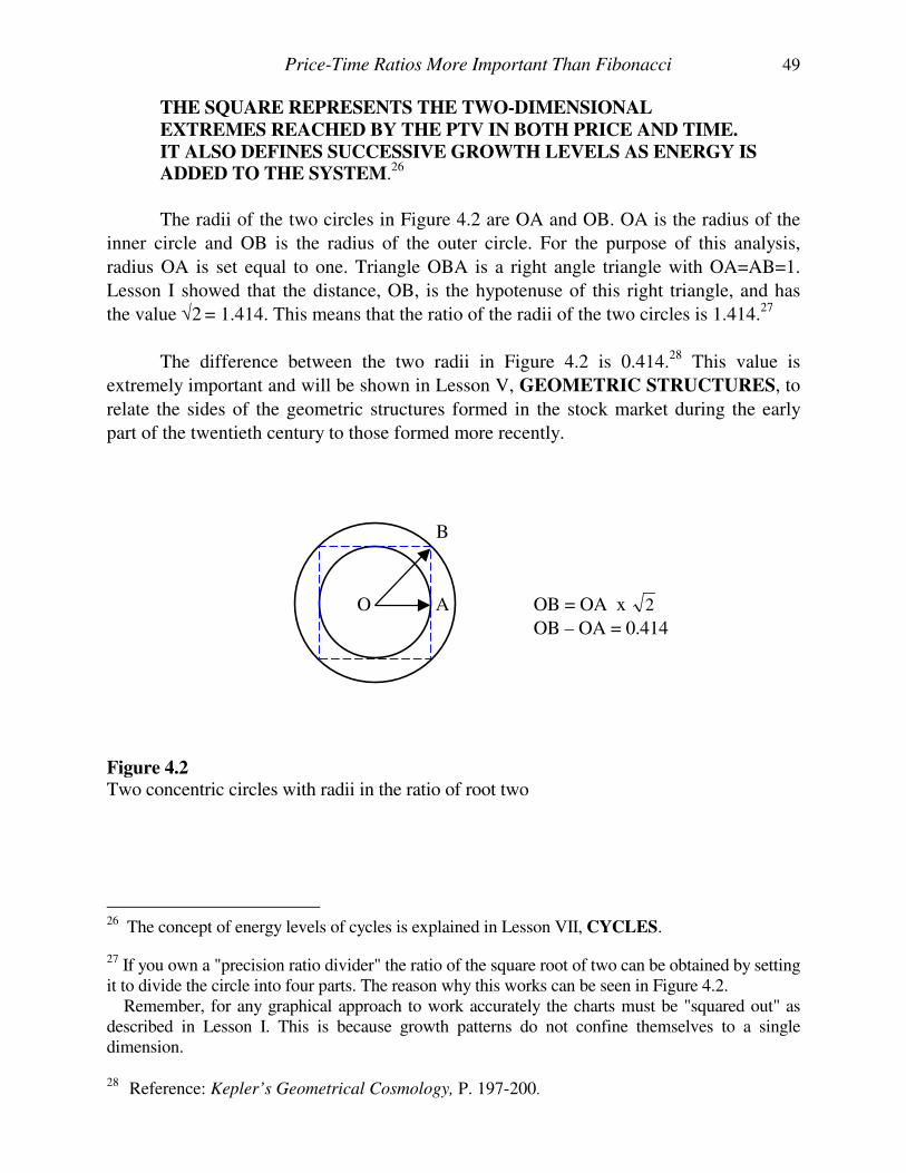
Price-Time Ratios More Important Than Fibonacci 49
THE SQUARE REPRESENTS THE TWO-DIMENSIONAL
EXTREMES REACHED BY THE PTV IN BOTH PRICE AND TIME.
IT ALSO DEFINES SUCCESSIVE GROWTH LEVELS AS ENERGY IS
ADDED TO THE SYSTEM.26
The radii of the two circles in Figure 4.2 are OA and OB. OA is the radius of the
inner circle and OB is the radius of the outer circle. For the purpose of this analysis,
radius OA is set equal to one. Triangle OBA is a right angle triangle with OA=AB=1.
Lesson I showed that the distance, OB, is the hypotenuse of this right triangle, and has
the value √2 = 1.414. This means that the ratio of the radii of the two circles is 1.414.27
The difference between the two radii in Figure 4.2 is 0.414.28 This value is
extremely important and will be shown in Lesson V, GEOMETRIC STRUCTURES, to
relate the sides of the geometric structures formed in the stock market during the early
part of the twentieth century to those formed more recently.
B
O A OB = OA x 2
OB – OA = 0.414
Figure 4.2
Two concentric circles with radii in the ratio of root two
26 The concept of energy levels of cycles is explained in Lesson VII, CYCLES.
27 If you own a "precision ratio divider" the ratio of the square root of two can be obtained by setting it to divide the circle into four parts. The reason why this works can be seen in Figure 4.2. Remember, for any graphical approach to work accurately the charts must be "squared out" as described in Lesson I. This is because growth patterns do not confine themselves to a single dimension.
28 Reference: Kepler’s Geometrical Cosmology, P. 197-200.
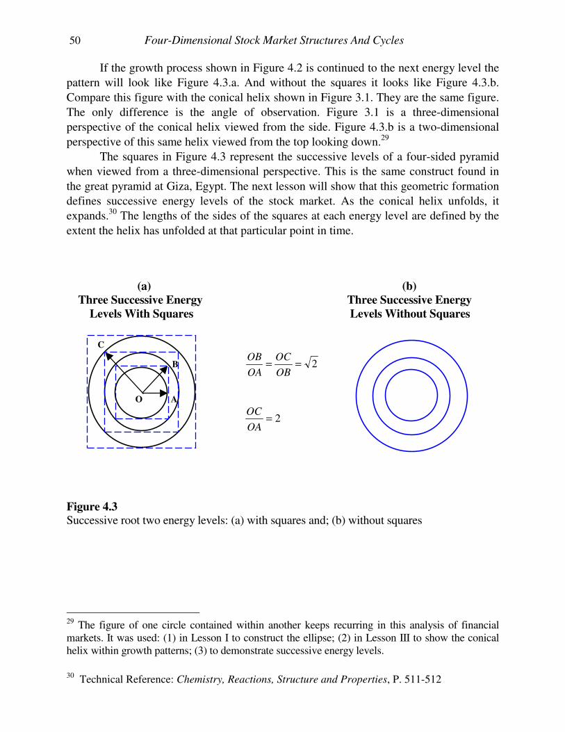
50 Four-Dimensional Stock Market Structures And Cycles
If the growth process shown in Figure 4.2 is continued to the next energy level the
pattern will look like Figure 4.3.a. And without the squares it looks like Figure 4.3.b.
Compare this figure with the conical helix shown in Figure 3.1. They are the same figure.
The only difference is the angle of observation. Figure 3.1 is a three-dimensional
perspective of the conical helix viewed from the side. Figure 4.3.b is a two-dimensional
perspective of this same helix viewed from the top looking down.29
The squares in Figure 4.3 represent the successive levels of a four-sided pyramid
when viewed from a three-dimensional perspective. This is the same construct found in
the great pyramid at Giza, Egypt. The next lesson will show that this geometric formation
defines successive energy levels of the stock market. As the conical helix unfolds, it
expands.30 The lengths of the sides of the squares at each energy level are defined by the
extent the helix has unfolded at that particular point in time.
(a) (b)
Three Successive Energy Three Successive Energy
Levels With Squares Levels Without Squares
C
B 2==OB
OC
OA
OB
O A
2=OA
OC
Figure 4.3 Successive root two energy levels: (a) with squares and; (b) without squares
29 The figure of one circle contained within another keeps recurring in this analysis of financial markets. It was used: (1) in Lesson I to construct the ellipse; (2) in Lesson III to show the conical helix within growth patterns; (3) to demonstrate successive energy levels.
30 Technical Reference: Chemistry, Reactions, Structure and Properties, P. 511-512
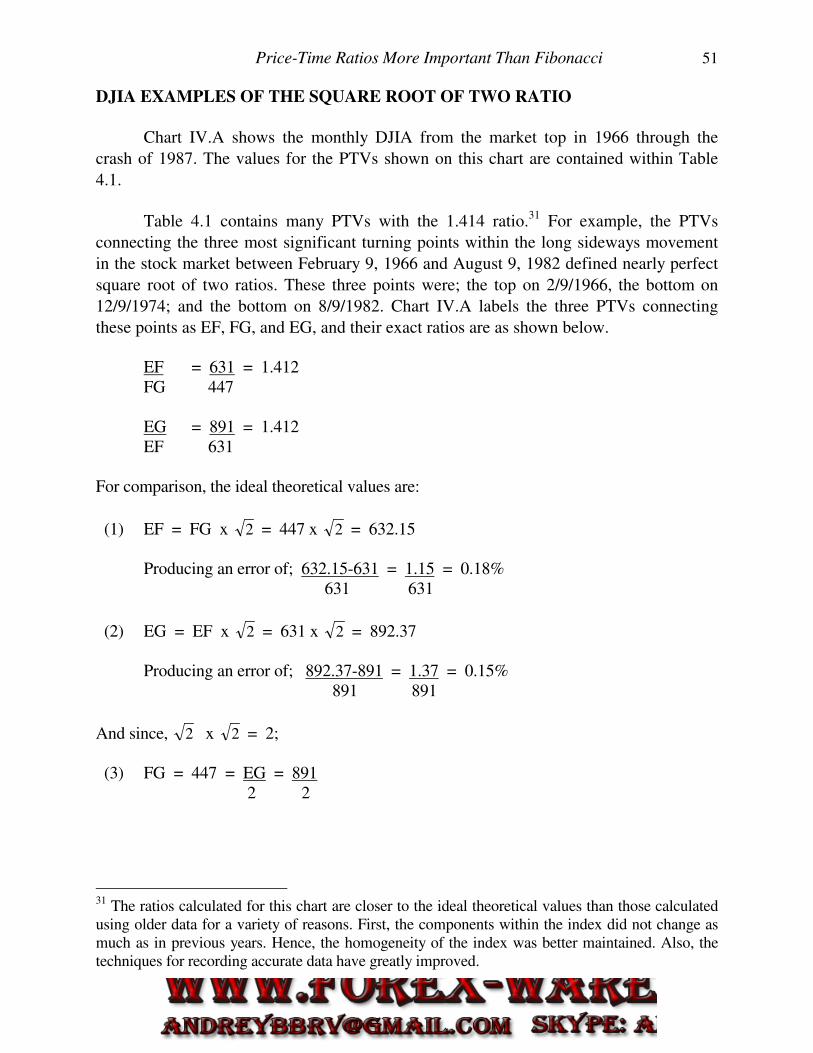
Price-Time Ratios More Important Than Fibonacci 51
DJIA EXAMPLES OF THE SQUARE ROOT OF TWO RATIO
Chart IV.A shows the monthly DJIA from the market top in 1966 through the
crash of 1987. The values for the PTVs shown on this chart are contained within Table
4.1.
Table 4.1 contains many PTVs with the 1.414 ratio.31 For example, the PTVs
connecting the three most significant turning points within the long sideways movement
in the stock market between February 9, 1966 and August 9, 1982 defined nearly perfect
square root of two ratios. These three points were; the top on 2/9/1966, the bottom on
12/9/1974; and the bottom on 8/9/1982. Chart IV.A labels the three PTVs connecting
these points as EF, FG, and EG, and their exact ratios are as shown below.
EF = 631 = 1.412 FG 447 EG = 891 = 1.412 EF 631 For comparison, the ideal theoretical values are:
(1) EF = FG x 2 = 447 x 2 = 632.15 Producing an error of; 632.15-631 = 1.15 = 0.18% 631 631
(2) EG = EF x 2 = 631 x 2 = 892.37 Producing an error of; 892.37-891 = 1.37 = 0.15% 891 891
And since, 2 x 2 = 2; (3) FG = 447 = EG = 891 2 2
31 The ratios calculated for this chart are closer to the ideal theoretical values than those calculated using older data for a variety of reasons. First, the components within the index did not change as much as in previous years. Hence, the homogeneity of the index was better maintained. Also, the techniques for recording accurate data have greatly improved.
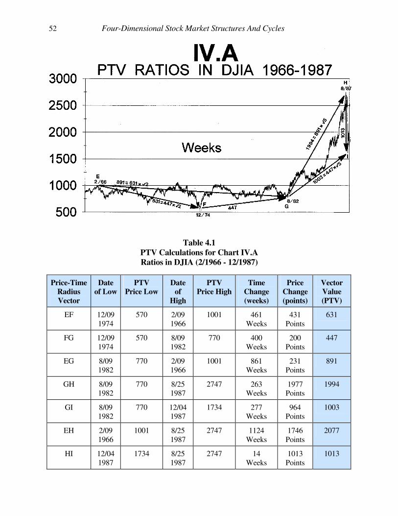
52 Four-Dimensional Stock Market Structures And Cycles
Table 4.1
PTV Calculations for Chart IV.A
Ratios in DJIA (2/1966 - 12/1987)
Price-Time
Radius
Vector
Date
of Low
PTV
Price Low
Date
of
High
PTV
Price High
Time
Change
(weeks)
Price
Change
(points)
Vector
Value
(PTV)
EF 12/09 1974
570 2/09 1966
1001 461 Weeks
431 Points
631
FG 12/09 1974
570 8/09 1982
770 400 Weeks
200 Points
447
EG 8/09 1982
770 2/09 1966
1001 861 Weeks
231 Points
891
GH 8/09 1982
770 8/25 1987
2747 263 Weeks
1977 Points
1994
GI 8/09 1982
770 12/04 1987
1734 277 Weeks
964 Points
1003
EH 2/09 1966
1001 8/25 1987
2747 1124 Weeks
1746 Points
2077
HI 12/04 1987
1734 8/25 1987
2747 14 Weeks
1013 Points
1013
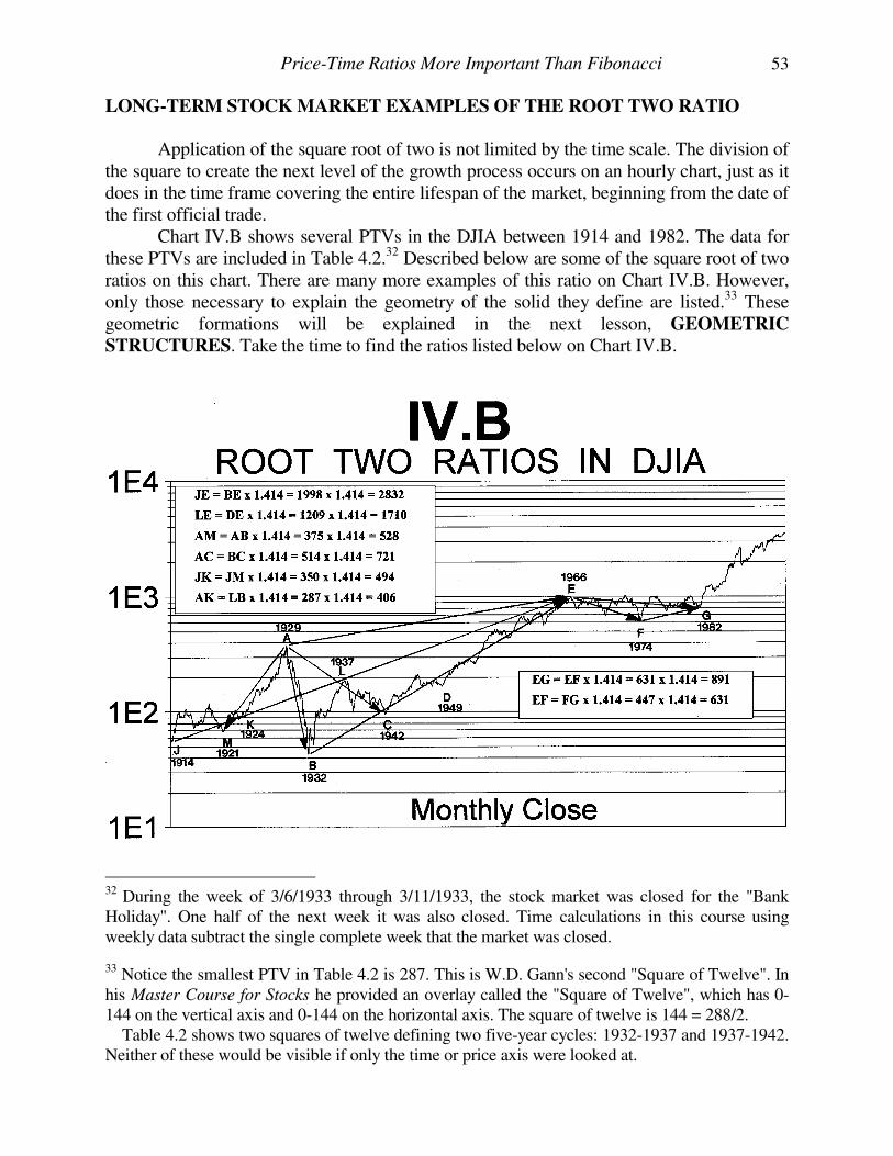
Price-Time Ratios More Important Than Fibonacci 53
LONG-TERM STOCK MARKET EXAMPLES OF THE ROOT TWO RATIO
Application of the square root of two is not limited by the time scale. The division of the square to create the next level of the growth process occurs on an hourly chart, just as it does in the time frame covering the entire lifespan of the market, beginning from the date of the first official trade. Chart IV.B shows several PTVs in the DJIA between 1914 and 1982. The data for these PTVs are included in Table 4.2.32 Described below are some of the square root of two ratios on this chart. There are many more examples of this ratio on Chart IV.B. However, only those necessary to explain the geometry of the solid they define are listed.33 These geometric formations will be explained in the next lesson, GEOMETRIC
STRUCTURES. Take the time to find the ratios listed below on Chart IV.B.
32 During the week of 3/6/1933 through 3/11/1933, the stock market was closed for the "Bank Holiday". One half of the next week it was also closed. Time calculations in this course using weekly data subtract the single complete week that the market was closed.
33 Notice the smallest PTV in Table 4.2 is 287. This is W.D. Gann's second "Square of Twelve". In his Master Course for Stocks he provided an overlay called the "Square of Twelve", which has 0-144 on the vertical axis and 0-144 on the horizontal axis. The square of twelve is 144 = 288/2. Table 4.2 shows two squares of twelve defining two five-year cycles: 1932-1937 and 1937-1942. Neither of these would be visible if only the time or price axis were looked at.
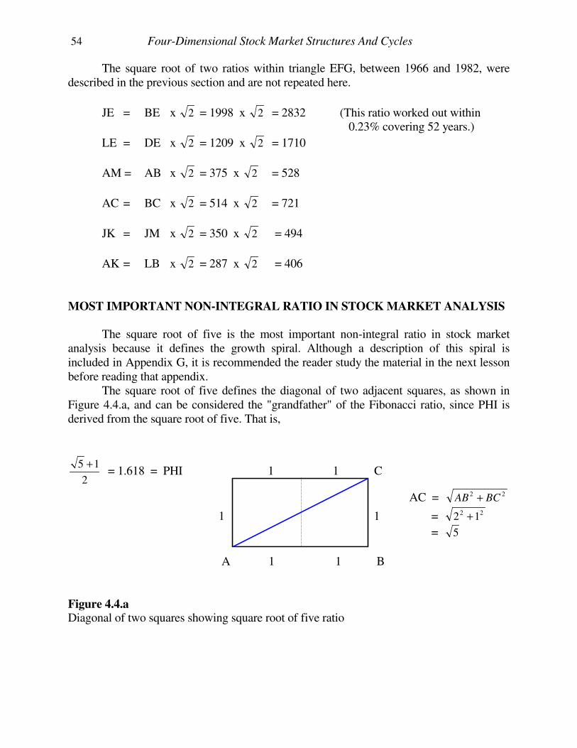
54 Four-Dimensional Stock Market Structures And Cycles
The square root of two ratios within triangle EFG, between 1966 and 1982, were described in the previous section and are not repeated here.
JE = BE x 2 = 1998 x 2 = 2832 (This ratio worked out within 0.23% covering 52 years.)
LE = DE x 2 = 1209 x 2 = 1710
AM = AB x 2 = 375 x 2 = 528
AC = BC x 2 = 514 x 2 = 721
JK = JM x 2 = 350 x 2 = 494
AK = LB x 2 = 287 x 2 = 406
MOST IMPORTANT NON-INTEGRAL RATIO IN STOCK MARKET ANALYSIS
The square root of five is the most important non-integral ratio in stock market analysis because it defines the growth spiral. Although a description of this spiral is included in Appendix G, it is recommended the reader study the material in the next lesson before reading that appendix. The square root of five defines the diagonal of two adjacent squares, as shown in Figure 4.4.a, and can be considered the "grandfather" of the Fibonacci ratio, since PHI is derived from the square root of five. That is,
2
15 + = 1.618 = PHI 1 1 C
AC = 22BCAB +
1 1 = 22 12 +
= 5
A 1 1 B
Figure 4.4.a Diagonal of two squares showing square root of five ratio
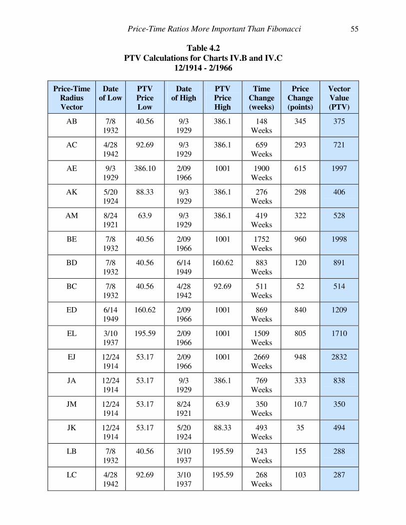
Price-Time Ratios More Important Than Fibonacci 55
Table 4.2
PTV Calculations for Charts IV.B and IV.C
12/1914 - 2/1966
Price-Time
Radius
Vector
Date
of Low
PTV
Price
Low
Date
of High
PTV
Price
High
Time
Change
(weeks)
Price
Change
(points)
Vector
Value
(PTV)
AB 7/8 1932
40.56 9/3 1929
386.1 148 Weeks
345 375
AC 4/28 1942
92.69 9/3 1929
386.1 659 Weeks
293 721
AE 9/3 1929
386.10 2/09 1966
1001 1900 Weeks
615 1997
AK 5/20 1924
88.33 9/3 1929
386.1 276 Weeks
298 406
AM 8/24 1921
63.9 9/3 1929
386.1 419 Weeks
322 528
BE 7/8 1932
40.56 2/09 1966
1001 1752 Weeks
960 1998
BD 7/8 1932
40.56 6/14 1949
160.62 883 Weeks
120 891
BC 7/8 1932
40.56 4/28 1942
92.69 511 Weeks
52 514
ED 6/14 1949
160.62 2/09 1966
1001 869 Weeks
840 1209
EL 3/10 1937
195.59 2/09 1966
1001 1509 Weeks
805 1710
EJ 12/24 1914
53.17 2/09 1966
1001 2669 Weeks
948 2832
JA 12/24 1914
53.17 9/3 1929
386.1 769 Weeks
333 838
JM 12/24 1914
53.17 8/24 1921
63.9 350 Weeks
10.7 350
JK 12/24 1914
53.17 5/20 1924
88.33 493 Weeks
35 494
LB 7/8 1932
40.56 3/10 1937
195.59 243 Weeks
155 288
LC 4/28 1942
92.69 3/10 1937
195.59 268 Weeks
103 287

56 Four-Dimensional Stock Market Structures And Cycles
The relationship between PHI and the square root of five is expressed geometrically in Figure 4.4.b, where PHI is derived from two adjacent squares, as was the square root of five in Figure 4.4.a. Figure 4.4.b is a double of Figure 3.3, which showed the Golden Section derived from the diagonal of the half square. Since the distances; AE = 3.236; and BD = 2; it follows,
AE = 3.236 = 1.618 1 1 BD 2 1 1 A B 1 C D E 2 1.618
3.236 = 5 + 1
Figure 4.4.b
Fibonacci ratio derived from two adjacent squares
DJIA EXAMPLES OF THE SQUARE ROOT OF FIVE RATIO
The 2.236 ratio is obvious when the PTVs from Chart IV.A are calculated, as in Table 4.1. This table shows GH, which extended from the low on August 9, 1982 to the top on August 25, 1987, to be a nearly exact 2.236 multiple of EG, which extended from the high on February 9, 1966 to the low on August 9, 1982. That is,
GH = 5 x EG
Therefore, GH is the diagonal of two adjacent squares that have side length equal to EG. To check the exact ratio between these two PTVs, GH is divided by EG; GH = 1994 = 2.238 EG 891 These PTVs span a time frame of over twenty-one years and still produce results with an error of less than two points. Accurately predicting a major market top that spanned a time frame of twenty-one years is quite an accomplishment. The ideal theoretical value for GH is given by;
GH = EG x 5 = 891 x 5 = 1992.34
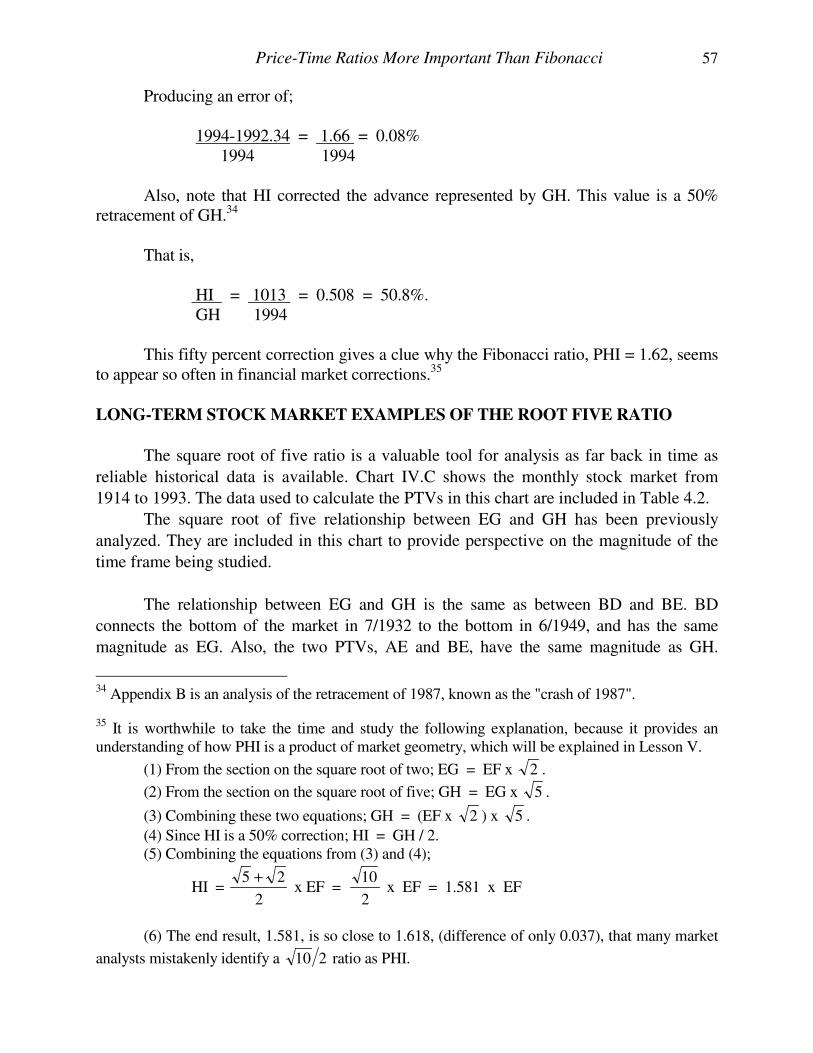
Price-Time Ratios More Important Than Fibonacci 57
Producing an error of; 1994-1992.34 = 1.66 = 0.08% 1994 1994 Also, note that HI corrected the advance represented by GH. This value is a 50% retracement of GH.34 That is, HI = 1013 = 0.508 = 50.8%. GH 1994 This fifty percent correction gives a clue why the Fibonacci ratio, PHI = 1.62, seems to appear so often in financial market corrections.35 LONG-TERM STOCK MARKET EXAMPLES OF THE ROOT FIVE RATIO
The square root of five ratio is a valuable tool for analysis as far back in time as
reliable historical data is available. Chart IV.C shows the monthly stock market from
1914 to 1993. The data used to calculate the PTVs in this chart are included in Table 4.2.
The square root of five relationship between EG and GH has been previously
analyzed. They are included in this chart to provide perspective on the magnitude of the
time frame being studied.
The relationship between EG and GH is the same as between BD and BE. BD
connects the bottom of the market in 7/1932 to the bottom in 6/1949, and has the same
magnitude as EG. Also, the two PTVs, AE and BE, have the same magnitude as GH.
34 Appendix B is an analysis of the retracement of 1987, known as the "crash of 1987".
35 It is worthwhile to take the time and study the following explanation, because it provides an understanding of how PHI is a product of market geometry, which will be explained in Lesson V.
(1) From the section on the square root of two; EG = EF x 2 .
(2) From the section on the square root of five; GH = EG x 5 .
(3) Combining these two equations; GH = (EF x 2 ) x 5 .
(4) Since HI is a 50% correction; HI = GH / 2. (5) Combining the equations from (3) and (4);
HI = 2
25 + x EF =
2
10 x EF = 1.581 x EF
(6) The end result, 1.581, is so close to 1.618, (difference of only 0.037), that many market
analysts mistakenly identify a 210 ratio as PHI.
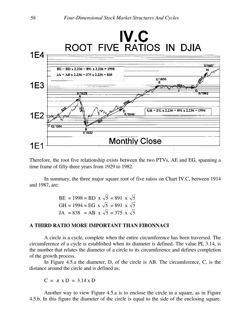
58 Four-Dimensional Stock Market Structures And Cycles
Therefore, the root five relationship exists between the two PTVs, AE and EG, spanning a
time frame of fifty-three years from 1929 to 1982. In summary, the three major square root of five ratios on Chart IV.C, between 1914 and 1987, are:
BE = 1998 = BD x 5 = 891 x 5
GH = 1994 = EG x 5 = 891 x 5
JA = 838 = AB x 5 = 375 x 5
A THIRD RATIO MORE IMPORTANT THAN FIBONNACI
A circle is a cycle, complete when the entire circumference has been traversed. The circumference of a cycle is established when its diameter is defined. The value PI, 3.14, is the number that relates the diameter of a circle to its circumference and defines completion of the growth process. In Figure 4.5.a the diameter, D, of the circle is AB. The circumference, C, is the distance around the circle and is defined as;
C = π x D = 3.14 x D Another way to view Figure 4.5.a is to enclose the circle in a square, as in Figure 4.5.b. In this figure the diameter of the circle is equal to the side of the enclosing square.
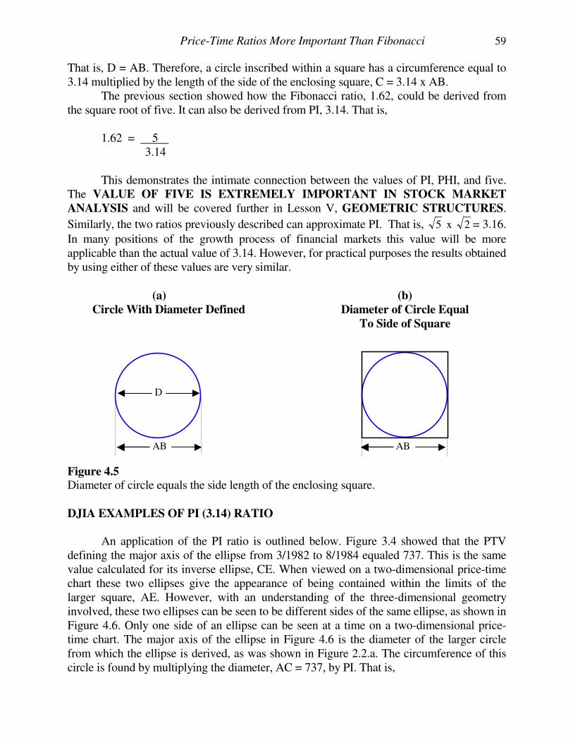
Price-Time Ratios More Important Than Fibonacci 59
That is, D = AB. Therefore, a circle inscribed within a square has a circumference equal to 3.14 multiplied by the length of the side of the enclosing square, C = 3.14 x AB. The previous section showed how the Fibonacci ratio, 1.62, could be derived from the square root of five. It can also be derived from PI, 3.14. That is, 1.62 = 5 3.14 This demonstrates the intimate connection between the values of PI, PHI, and five. The VALUE OF FIVE IS EXTREMELY IMPORTANT IN STOCK MARKET
ANALYSIS and will be covered further in Lesson V, GEOMETRIC STRUCTURES.
Similarly, the two ratios previously described can approximate PI. That is, 5 x 2 = 3.16.
In many positions of the growth process of financial markets this value will be more applicable than the actual value of 3.14. However, for practical purposes the results obtained by using either of these values are very similar.
(a)
Circle With Diameter Defined
D
(b)
Diameter of Circle Equal
To Side of Square
AB AB Figure 4.5 Diameter of circle equals the side length of the enclosing square.
DJIA EXAMPLES OF PI (3.14) RATIO
An application of the PI ratio is outlined below. Figure 3.4 showed that the PTV defining the major axis of the ellipse from 3/1982 to 8/1984 equaled 737. This is the same value calculated for its inverse ellipse, CE. When viewed on a two-dimensional price-time chart these two ellipses give the appearance of being contained within the limits of the larger square, AE. However, with an understanding of the three-dimensional geometry involved, these two ellipses can be seen to be different sides of the same ellipse, as shown in Figure 4.6. Only one side of an ellipse can be seen at a time on a two-dimensional price-time chart. The major axis of the ellipse in Figure 4.6 is the diameter of the larger circle from which the ellipse is derived, as was shown in Figure 2.2.a. The circumference of this circle is found by multiplying the diameter, AC = 737, by PI. That is,
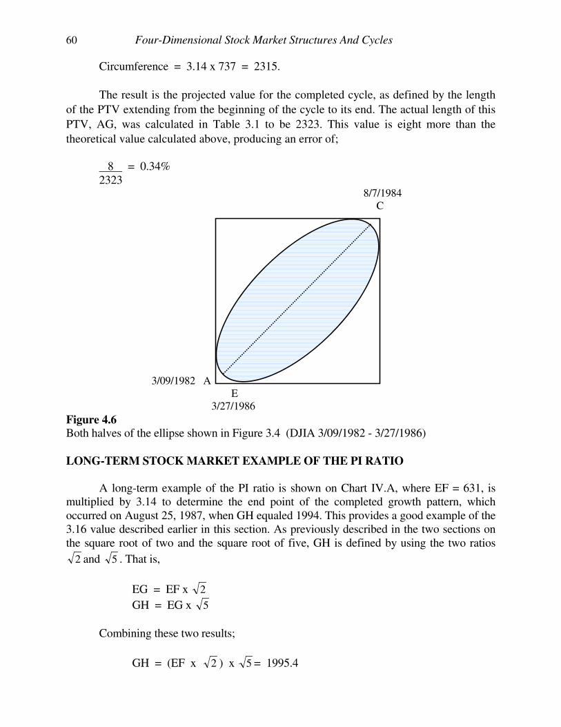
60 Four-Dimensional Stock Market Structures And Cycles
Circumference = 3.14 x 737 = 2315.
The result is the projected value for the completed cycle, as defined by the length
of the PTV extending from the beginning of the cycle to its end. The actual length of this
PTV, AG, was calculated in Table 3.1 to be 2323. This value is eight more than the
theoretical value calculated above, producing an error of; 8 = 0.34% 2323 8/7/1984
C
3/09/1982 A E 3/27/1986
Figure 4.6 Both halves of the ellipse shown in Figure 3.4 (DJIA 3/09/1982 - 3/27/1986)
LONG-TERM STOCK MARKET EXAMPLE OF THE PI RATIO
A long-term example of the PI ratio is shown on Chart IV.A, where EF = 631, is multiplied by 3.14 to determine the end point of the completed growth pattern, which occurred on August 25, 1987, when GH equaled 1994. This provides a good example of the 3.16 value described earlier in this section. As previously described in the two sections on the square root of two and the square root of five, GH is defined by using the two ratios
2 and 5 . That is,
EG = EF x 2
GH = EG x 5 Combining these two results;
GH = (EF x 2 ) x 5 = 1995.4
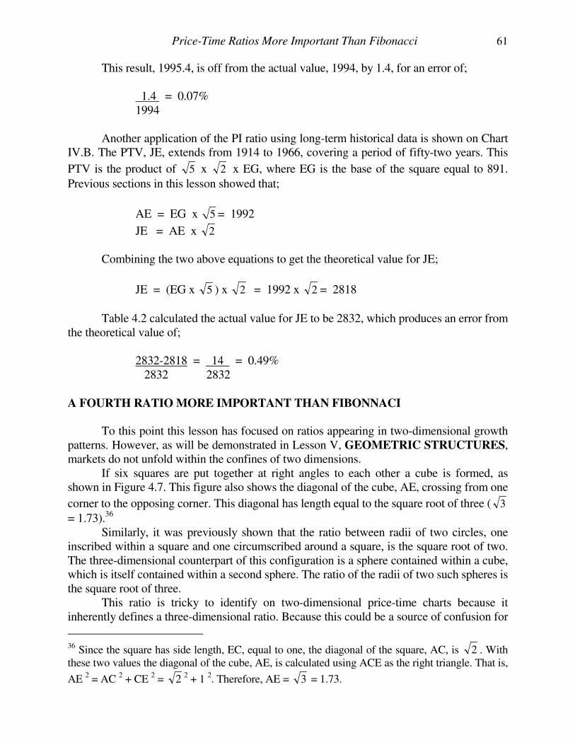
Price-Time Ratios More Important Than Fibonacci 61
This result, 1995.4, is off from the actual value, 1994, by 1.4, for an error of; 1.4 = 0.07% 1994 Another application of the PI ratio using long-term historical data is shown on Chart IV.B. The PTV, JE, extends from 1914 to 1966, covering a period of fifty-two years. This
PTV is the product of 5 x 2 x EG, where EG is the base of the square equal to 891.
Previous sections in this lesson showed that;
AE = EG x 5 = 1992
JE = AE x 2
Combining the two above equations to get the theoretical value for JE;
JE = (EG x 5 ) x 2 = 1992 x 2 = 2818
Table 4.2 calculated the actual value for JE to be 2832, which produces an error from the theoretical value of; 2832-2818 = 14 = 0.49% 2832 2832
A FOURTH RATIO MORE IMPORTANT THAN FIBONNACI
To this point this lesson has focused on ratios appearing in two-dimensional growth patterns. However, as will be demonstrated in Lesson V, GEOMETRIC STRUCTURES, markets do not unfold within the confines of two dimensions. If six squares are put together at right angles to each other a cube is formed, as shown in Figure 4.7. This figure also shows the diagonal of the cube, AE, crossing from one
corner to the opposing corner. This diagonal has length equal to the square root of three ( 3
= 1.73).36 Similarly, it was previously shown that the ratio between radii of two circles, one inscribed within a square and one circumscribed around a square, is the square root of two. The three-dimensional counterpart of this configuration is a sphere contained within a cube, which is itself contained within a second sphere. The ratio of the radii of two such spheres is the square root of three. This ratio is tricky to identify on two-dimensional price-time charts because it inherently defines a three-dimensional ratio. Because this could be a source of confusion for
36 Since the square has side length, EC, equal to one, the diagonal of the square, AC, is 2 . With these two values the diagonal of the cube, AE, is calculated using ACE as the right triangle. That is,
AE 2 = AC 2 + CE 2 = 2 2 + 1 2. Therefore, AE = 3 = 1.73.
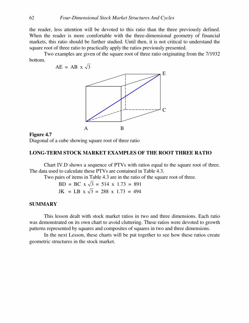
62 Four-Dimensional Stock Market Structures And Cycles
the reader, less attention will be devoted to this ratio than the three previously defined. When the reader is more comfortable with the three-dimensional geometry of financial markets, this ratio should be further studied. Until then, it is not critical to understand the square root of three ratio to practically apply the ratios previously presented. Two examples are given of the square root of three ratio originating from the 7/1932 bottom.
AE = AB x 3
E C A B Figure 4.7
Diagonal of a cube showing square root of three ratio
LONG-TERM STOCK MARKET EXAMPLES OF THE ROOT THREE RATIO
Chart IV.D shows a sequence of PTVs with ratios equal to the square root of three. The data used to calculate these PTVs are contained in Table 4.3. Two pairs of items in Table 4.3 are in the ratio of the square root of three.
BD = BC x 3 = 514 x 1.73 = 891
JK = LB x 3 = 288 x 1.73 = 494
SUMMARY
This lesson dealt with stock market ratios in two and three dimensions. Each ratio was demonstrated on its own chart to avoid cluttering. These ratios were devoted to growth patterns represented by squares and composites of squares in two and three dimensions.
In the next Lesson, these charts will be put together to see how these ratios create
geometric structures in the stock market.
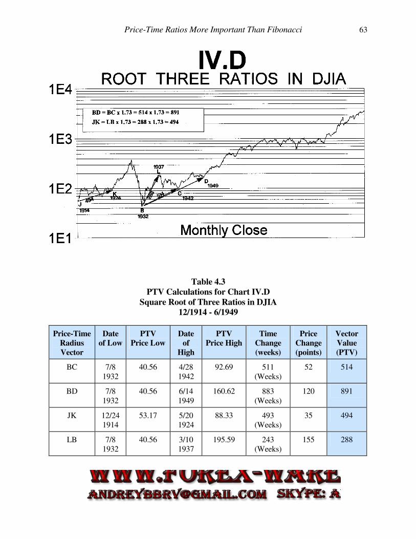
Price-Time Ratios More Important Than Fibonacci 63
Table 4.3
PTV Calculations for Chart IV.D
Square Root of Three Ratios in DJIA
12/1914 - 6/1949
Price-Time
Radius
Vector
Date
of Low
PTV
Price Low
Date
of
High
PTV
Price High
Time
Change
(weeks)
Price
Change
(points)
Vector
Value
(PTV)
BC 7/8 1932
40.56 4/28 1942
92.69 511 (Weeks)
52 514
BD 7/8 1932
40.56 6/14 1949
160.62 883 (Weeks)
120 891
JK 12/24 1914
53.17 5/20 1924
88.33 493 (Weeks)
35 494
LB
7/8 1932
40.56 3/10 1937
195.59 243 (Weeks)
155 288
LESSON V
GEOMETRIC STRUCTURES
Geometry existed before the Creation, it is co-eternal with the mind of God, is God himself.
Johannes Kepler (1630 A.D.) ...Harmonice Mundi (Harmony of the World)
INTRODUCTION
Previous lessons explained the multi-dimensional nature of price-time. This lesson will provide additional proof of this powerful concept, as price-time charts will be shown to be nothing more than a two-dimensional sequential recording of geometric solids in motion. Financial markets unfold in price-time within the confines of predetermined points of force. The relative locations of these points in three dimensions form geometric structures. This phenomenon is not unique to financial markets. Matter creates clearly defined geometric structures when it attains a stable state. Geologists apply the "crystal lattice" structure to classify minerals by looking at the geometric arrangement of their planes of cleavage. Similarly, chemists can identify an element by looking at the geometry of its constituent atoms.37 These applications are nothing more than simple three-dimensional geometry. As previously explained, financial markets are not exempt from natural law, including this one. The reader may have had the opportunity in the past to try a puzzle where he imagined what figure is created when a piece of paper is folded along a variety of dotted lines. This type of mental exercise requires using the abstract or right hemisphere of the brain. There is very little in modern academia that encourages the development of this ability. In fact, our whole western civilization is primarily based upon usage of the logical or left hemisphere of the brain. In western society if a conclusion cannot be logically derived it is presumed fallacious. This is not the case throughout the world. Several eastern societies demonstrate an emphasis on "intuitive wisdom", or conclusions that are not limited by the sequential derivation required of the left hemisphere of the brain. In the sixth century B.C. the Chinese philosopher, Lao Tzu, wrote the work Tao Te Ching, which was intentionally styled to demand an intuitive conceptualization of reality.38 In fact, this philosophy held a certain
contempt for logical reasoning, considering it part of an artificial world created by man.
37 Technical References: Chemistry, Reactions, Structures and Properties, P. 500-504,
Fundamentals of Physics, P. 309, 948.
38 The limited records during this time make it impossible to attribute to Lao Tzu the entire writing of Tao Te Ching, which literally translates as "Classic of the Way and Power". Contemporary thought is that other authors over a period of time contributed to this work. Lao Tzu, whose name means "Old Master", originated the philosophy of Taoism.
Geometric Structures 65
Referring to Taoism, the philosopher, Chuang Tzu, stated in 400 B.C.; "The most extensive knowledge does not necessarily know it; reasoning will
not make men wise in it. The sages have decided against both these methods." In this lesson the reader will use his abilities of abstraction to see the geometric patterns unfolding in the stock market. If this seems difficult at first, do not despair. This type of thinking has been practiced for centuries, and a little mental work will make this exercise much easier.
TWO-DIMENSIONAL GEOMETRY
This discussion of two-dimensional geometry is valuable as a first step to understanding true four-dimensional market geometry. As will be explained in the section on three-dimensional geometry, ONE SIDE OF THE GEOMETRIC STRUCTURE IS
VISIBLE IN OUR PERCEPTION AT A TIME.
The limitation of a two-dimensional analysis of price-time charts is seen during
the period when one side of the geometric structure completes and the entire structure
appears to rotate to expose the new face. These are the periods when financial market
analysts are most confused. The cycles they have been following suddenly "disappear",
and a seemingly new set of cycles replaces them. These analysts find themselves waiting
for cycle bottoms or tops that never arrive. To understand the transition between two-
dimensional faces, three-dimensional geometry must be studied. The relationships
between the sides of these three-dimensional structures are predictable if the nature of the
complete geometric structure is understood. Three-dimensional geometry will be
explained later in this lesson. First, a certain amount of background knowledge must be
developed in the form of two-dimensional geometry.
When a living cell reproduces it internally divides in half, creating a condition where
each new cell has half the area of the original cell. The cells then separate and grow to
maturity with an area equal to that of the original cell. This process of fission creates two
cells with a combined area twice the original cell.
Geometrically, this process of division is represented in Figure 5.1.a, where square
ABC is the original area beginning the division process by dividing in half along diagonal,
AC. As described in Lesson IV, PRICE-TIME RATIOS MORE IMPORTANT THAN
FIBONACCI, this diagonal has length 1.414 times the side of the square, AB. The diagonal
is the longest line that can be used within the square to divide it into two equal parts. 39 To create a square with twice the area of the original the diagonal, AC, of square AB is used as a side of the new square, ACDE, in Figure 5.1.b. Since the side of the new square
39 References: Connections – The Geometric Bridge Between Art and Science, P. 451;
Sacred Geometry
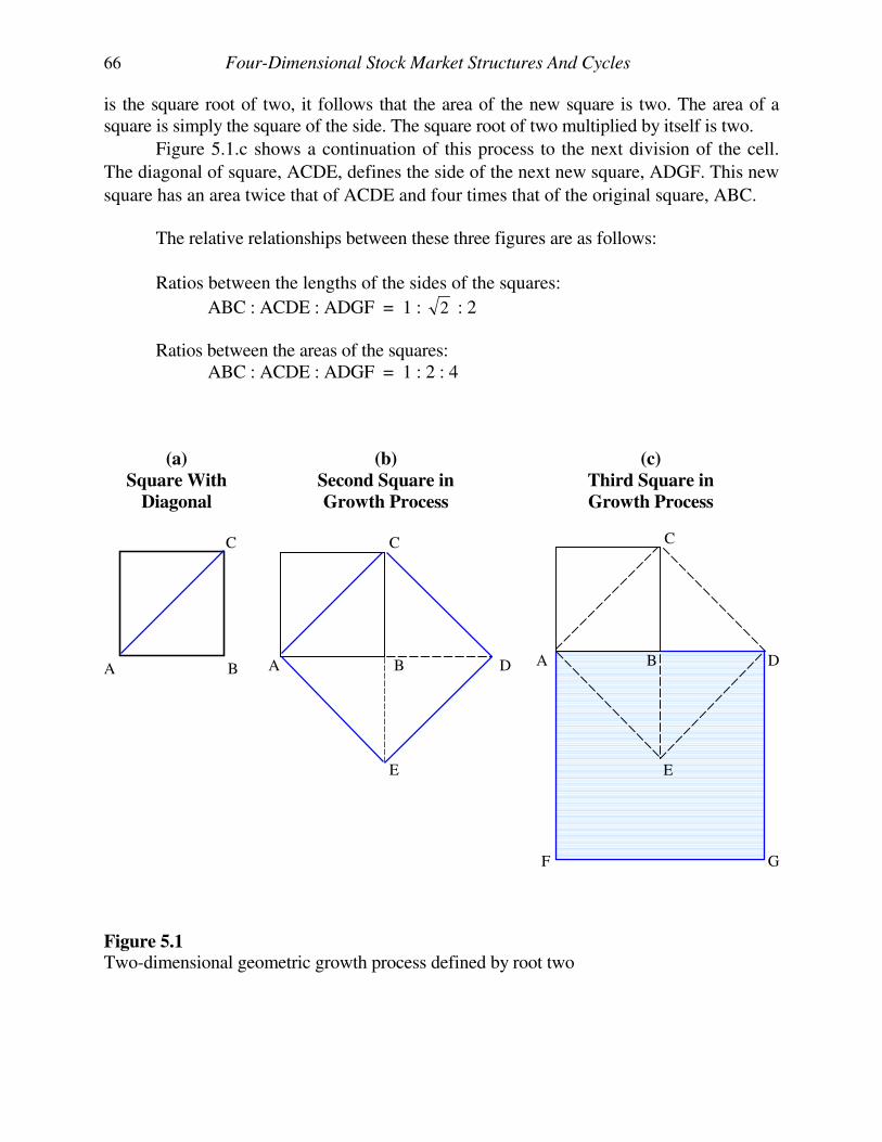
66 Four-Dimensional Stock Market Structures And Cycles
is the square root of two, it follows that the area of the new square is two. The area of a
square is simply the square of the side. The square root of two multiplied by itself is two.
Figure 5.1.c shows a continuation of this process to the next division of the cell.
The diagonal of square, ACDE, defines the side of the next new square, ADGF. This new
square has an area twice that of ACDE and four times that of the original square, ABC.
The relative relationships between these three figures are as follows:
Ratios between the lengths of the sides of the squares:
ABC : ACDE : ADGF = 1 : 2 : 2 Ratios between the areas of the squares: ABC : ACDE : ADGF = 1 : 2 : 4
(a)
Square With
Diagonal
C
A B
(b)
Second Square in
Growth Process C
A B D
E
(c)
Third Square in
Growth Process
C
A B D E F G
Figure 5.1 Two-dimensional geometric growth process defined by root two
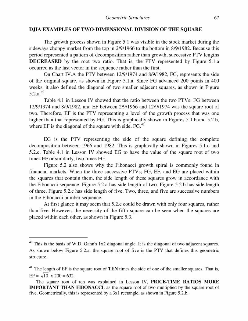
Geometric Structures 67
DJIA EXAMPLES OF TWO-DIMENSIONAL DIVISION OF THE SQUARE
The growth process shown in Figure 5.1 was visible in the stock market during the
sideways choppy market from the top in 2/9/1966 to the bottom in 8/9/1982. Because this
period represented a pattern of decomposition rather than growth, successive PTV lengths
DECREASED by the root two ratio. That is, the PTV represented by Figure 5.1.a
occurred as the last vector in the sequence rather than the first.
On Chart IV.A the PTV between 12/9/1974 and 8/9/1982, FG, represents the side
of the original square, as shown in Figure 5.1.a. Since FG advanced 200 points in 400
weeks, it also defined the diagonal of two smaller adjacent squares, as shown in Figure
5.2.a.40
Table 4.1 in Lesson IV showed that the ratio between the two PTVs: FG between
12/9/1974 and 8/9/1982, and EF between 2/9/1966 and 12/9/1974 was the square root of
two. Therefore, EF is the PTV representing a level of the growth process that was one
higher than that represented by FG. This is graphically shown in Figures 5.1.b and 5.2.b,
where EF is the diagonal of the square with side, FG.41
EG is the PTV representing the side of the square defining the complete
decomposition between 1966 and 1982. This is graphically shown in Figures 5.1.c and
5.2.c. Table 4.1 in Lesson IV showed EG to have the value of the square root of two
times EF or similarly, two times FG.
Figure 5.2 also shows why the Fibonacci growth spiral is commonly found in
financial markets. When the three successive PTVs; FG, EF, and EG are placed within
the squares that contain them, the side length of these squares grow in accordance with
the Fibonacci sequence. Figure 5.2.a has side length of two. Figure 5.2.b has side length
of three. Figure 5.2.c has side length of five. Two, three, and five are successive numbers
in the Fibonacci number sequence.
At first glance it may seem that 5.2.c could be drawn with only four squares, rather
than five. However, the necessity of the fifth square can be seen when the squares are
placed within each other, as shown in Figure 5.3.
40 This is the basis of W.D. Gann's 1x2 diagonal angle. It is the diagonal of two adjacent squares.
As shown below Figure 5.2.a, the square root of five is the PTV that defines this geometric
structure.
41 The length of EF is the square root of TEN times the side of one of the smaller squares. That is,
EF = 10 x 200 = 632.
The square root of ten was explained in Lesson IV, PRICE-TIME RATIOS MORE
IMPORTANT THAN FIBONACCI, as the square root of two multiplied by the square root of five. Geometrically, this is represented by a 3x1 rectangle, as shown in Figure 5.2.b.
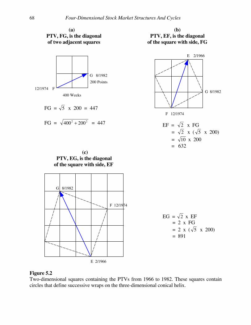
68 Four-Dimensional Stock Market Structures And Cycles
(a)
PTV, FG, is the diagonal of two adjacent squares
G 8/1982
200 Points
12/1974 F
400 Weeks
FG = 5 x 200 = 447
FG = 22 200400 + = 447
(b)
PTV, EF, is the diagonal
of the square with side, FG
E 2/1966
G 8/1982
F 12/1974
EF = 2 x FG
= 2 x ( 5 x 200)
= 10 x 200
= 632
(c)
PTV, EG, is the diagonal
of the square with side, EF G 8/1982
F 12/1974
EG = 2 x EF = 2 x FG
= 2 x ( 5 x 200)
= 891
E 2/1966
Figure 5.2
Two-dimensional squares containing the PTVs from 1966 to 1982. These squares contain circles that define successive wraps on the three-dimensional conical helix.
Geometric Structures 69
Figure 5.3 combines the three squares from Figure 5.2 into one figure, and shows the relative growth of the magnitudes of the respective PTVs. The ratios between these PTVs display a square root of two geometric proportion. Each of these radii vectors define the interval of operation within the growth phase taking place within that square. After each growth phase completes, the next radius vector defines the next interval. If the growth process is that of decomposition, as it was during the period between 1966 and 1982, the larger radius vector, EG, decomposes by the root two proportion until decomposition is complete. The decomposition between the dates 1966 and 1982 was complete when radius vector FG completed on August 9, 1982 with a proportion to the preceding vectors, EF and EG, in the ratio of the square root of two. The period between 1929 and 1932 also represented decomposition of the growth process taking place at that time. The length of the PTV during the decline between 1929 and 1932 was equal to the length of the PTV during the preceding advance from 1921 to 1929, divided by the square root of two. This is shown in Figure 5.4 where the two PTVs, AB and MA, are shown to be in the ratio of the square root of two.
The square shown in Figure 5.2.c extended from 1966 to 1982. This square is one
face of a four-dimensional structure, which is reflected onto two dimensions in price-time
charts. Only one face of this four-dimensional structure is visible at a time as it rotates
into view. Price-time charts provide a convenient historic record of each of these faces as
they present themselves.
Figure 5.3
Combined radii vectors EF, FG, EG from Figure 5.2, showing root two progression in the lengths of the PTVs between 1966 and 1982
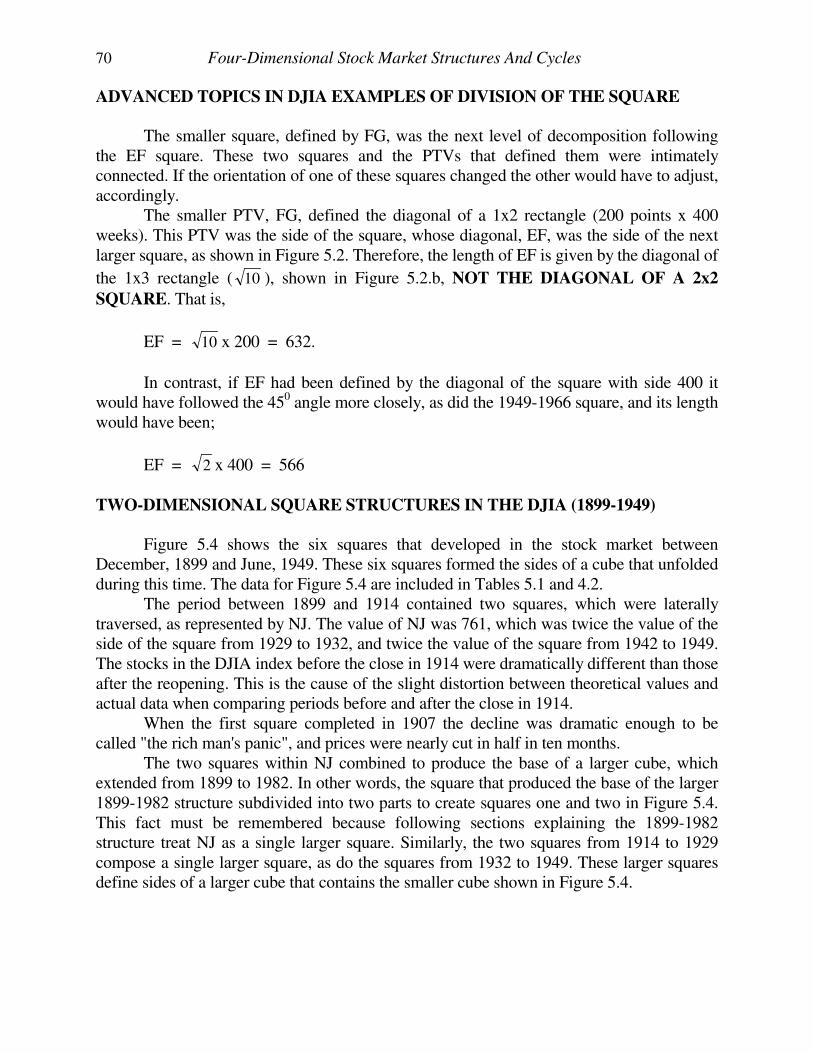
70 Four-Dimensional Stock Market Structures And Cycles
ADVANCED TOPICS IN DJIA EXAMPLES OF DIVISION OF THE SQUARE
The smaller square, defined by FG, was the next level of decomposition following the EF square. These two squares and the PTVs that defined them were intimately connected. If the orientation of one of these squares changed the other would have to adjust, accordingly. The smaller PTV, FG, defined the diagonal of a 1x2 rectangle (200 points x 400 weeks). This PTV was the side of the square, whose diagonal, EF, was the side of the next larger square, as shown in Figure 5.2. Therefore, the length of EF is given by the diagonal of
the 1x3 rectangle ( 10 ), shown in Figure 5.2.b, NOT THE DIAGONAL OF A 2x2
SQUARE. That is,
EF = 10 x 200 = 632.
In contrast, if EF had been defined by the diagonal of the square with side 400 it would have followed the 450 angle more closely, as did the 1949-1966 square, and its length would have been;
EF = 2 x 400 = 566 TWO-DIMENSIONAL SQUARE STRUCTURES IN THE DJIA (1899-1949)
Figure 5.4 shows the six squares that developed in the stock market between December, 1899 and June, 1949. These six squares formed the sides of a cube that unfolded during this time. The data for Figure 5.4 are included in Tables 5.1 and 4.2. The period between 1899 and 1914 contained two squares, which were laterally traversed, as represented by NJ. The value of NJ was 761, which was twice the value of the side of the square from 1929 to 1932, and twice the value of the square from 1942 to 1949. The stocks in the DJIA index before the close in 1914 were dramatically different than those after the reopening. This is the cause of the slight distortion between theoretical values and actual data when comparing periods before and after the close in 1914. When the first square completed in 1907 the decline was dramatic enough to be called "the rich man's panic", and prices were nearly cut in half in ten months. The two squares within NJ combined to produce the base of a larger cube, which extended from 1899 to 1982. In other words, the square that produced the base of the larger 1899-1982 structure subdivided into two parts to create squares one and two in Figure 5.4. This fact must be remembered because following sections explaining the 1899-1982 structure treat NJ as a single larger square. Similarly, the two squares from 1914 to 1929 compose a single larger square, as do the squares from 1932 to 1949. These larger squares define sides of a larger cube that contains the smaller cube shown in Figure 5.4.
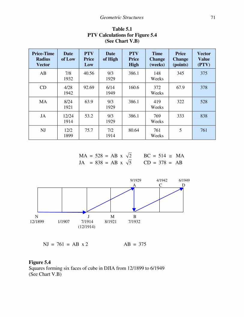
Geometric Structures 71
Table 5.1
PTV Calculations for Figure 5.4
(See Chart V.B)
Price-Time
Radius
Vector
Date
of Low
PTV
Price
Low
Date
of High
PTV
Price
High
Time
Change
(weeks)
Price
Change
(points)
Vector
Value
(PTV)
AB 7/8 1932
40.56 9/3 1929
386.1 148 Weeks
345 375
CD 4/28 1942
92.69 6/14 1949
160.6 372 Weeks
67.9 378
MA 8/24 1921
63.9 9/3 1929
386.1 419 Weeks
322 528
JA 12/24 1914
53.2 9/3 1929
386.1 769 Weeks
333 838
NJ 12/2 1899
75.7 7/2 1914
80.64 761 Weeks
5 761
MA = 528 = AB x 2 BC = 514 ≅ MA
JA = 838 = AB x 5 CD = 378 = AB
9/1929 4/1942 6/1949
A C D
N J M B 12/1899 1/1907 7/1914 8/1921 7/1932 (12/1914)
NJ = 761 = AB x 2 AB = 375 Figure 5.4
Squares forming six faces of cube in DJIA from 12/1899 to 6/1949 (See Chart V.B)
72 Four-Dimensional Stock Market Structures And Cycles
Because the market was closed between 7/31/1914 and 12/12/1914, NJ terminated in 7/1914 and JA began in 12/1914. Between 1914 and 1929 two squares completed. The size of these squares equaled the two squares between 1899 and 1914. The action within the 1921-1929 square differed from the three preceding it by crossing the square diagonally. From Table 5.1 it can be seen that the length of the side of the squares during this time period was 375. That is, AB equaled 375, CD equaled 378, and twice this amount, 761, was expended in the dimension of time between 1899 and 1914. Since it is known that the length of the side of the square during this time was 375, it follows that a diagonal of one of these squares is given by the square root of two ratio. That is,
Diagonal of a square in Figure 5.4 = 2 x 375 = 530 This is the value of MA from the bottom on 8/24/1921 to the top on 9/3/1929. The error between the actual value of MA and the ideal theoretical value, calculated above, is; 530 - 528 = 2 = 0.38% 530 530
Figure 4.4.a showed that the diagonal of two adjacent squares is 5 times the length
of the side of one of the squares. Therefore, it follows that JA, which is the diagonal of the two squares from the bottom on 12/24/1914 to the top on 9/3/1929 must equal:
Diagonal of two squares in Figure 5.4 = 5 x 375 = 838
This theoretical value matched the actual data perfectly. The diagonal of the two squares represented by JA is shown in Figure 5.4 to be 838.42 Analysts applying the traditional "Gann angles" of 450 and 1x2 to two-dimensional price-time charts are not aware of the geometric arrangement outlined above. This is because the diagonal of the square, MA, did not follow the 450 angle. Nor did the diagonal of two squares, JA, follow the 1x2 angle. Similarly, Gann analysts drawing the 1x2 angle from the 9/3/1929 top see the action consistently drop below that angle. Between 1929 and 1932 the market dropped 345 points in 148 weeks. In contrast, the 1x2 angle dropped 296
points during this same time frame. The reason the action did not follow the ideal angles is:
42 Appendix G provides a closer look at the growth spiral that defined the squares formed between 1921 and 1932. It is recommended the reader reference that material at this time.
Geometric Structures 73
PRICE-TIME ACTION WITHIN A SQUARE ONLY FOLLOWS THE
1x2, 450, OR 2x1 ANGLES IF THE ORIENTATION OF THE SQUARE
IS ITSELF SQUARE WITH THE PRICE AND TIME AXES OF THE
CHART. IF THE SQUARE CONTAINING THE ACTION IS
ROTATED EITHER DIRECTION WITH RESPECT TO THE AXES
OF THE CHART, THE ANGLES WITHIN THAT SQUARE ARE
ALSO ROTATED, ACCORDINGLY.
The orientation of the squares containing the action between 1914 and 1932 was rotated in a clockwise direction. Appendix G showed that the relative orientation of the two PTVs, JA and AB, was fixed by the square root of five growth spiral. Consequently, the angles followed by these two PTVs were fixed relative to each other, and not the price and time axes of the chart. This is further evidence that true geometric configurations remain unseen unless the action is viewed from a perspective not limited to a single dimension. Analysis using PTVs provides such a perspective.
TWO-DIMENSIONAL SQUARE STRUCTURES IN THE DJIA (1932-1987)
If the squares defining the market activity from the bottom in 7/1932 until after the crash of 10/1987 are placed together, the two-dimensional structure shown in Figure 5.5 is produced. The data for the PTVs in this figure are contained in Tables 4.1 and 4.2. In this figure it is seen that BE, from 1932 to 1966, has the same length as GH, from 8/1982 to 8/1987.43 Both these PTVs represent diagonals of two adjacent squares, which had side length equal to 891. Hence, their magnitude is given by the square root of five ratio. That is,
GH = BE = 1994 = 5 x 891
This ratio was calculated in the previous lesson, PRICE-TIME RATIOS MORE
IMPORTANT THAN FIBONACCI. Refer to that lesson for the calculation of the small error between the actual and the ideal theoretical values.
The difference between the two squares represented by GH and BE is that one
took 34 years to work out and the other took only 5 years. This is possible because the
1932 to 1966 squares are lying next to each other, and the 1982 to 1987 squares are
stacked on top of each other. This can be seen in Figure 3.4, where the rectangle lying
flat, AC, was formed early in the growth process when the exponential curve was
relatively flat. As the curve arcs upward the squares defining the price-time action stack
on top of each other, such as CE in Figure 3.4, rather than next to each other as they do
early in the growth process.
43 Compare Figure 5.5 with Figure 3.4, which showed two 3x2 rectangles at different points in the growth process.
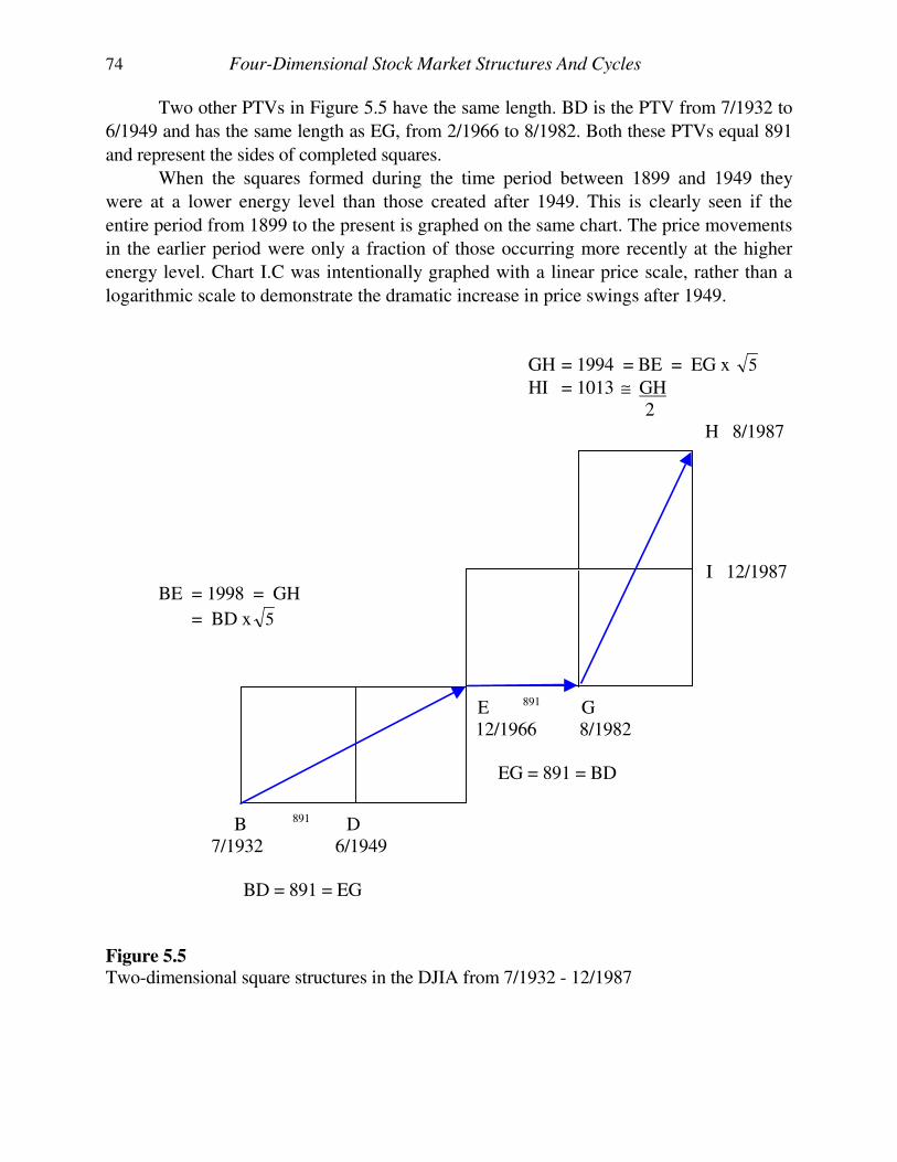
74 Four-Dimensional Stock Market Structures And Cycles
Two other PTVs in Figure 5.5 have the same length. BD is the PTV from 7/1932 to
6/1949 and has the same length as EG, from 2/1966 to 8/1982. Both these PTVs equal 891
and represent the sides of completed squares.
When the squares formed during the time period between 1899 and 1949 they
were at a lower energy level than those created after 1949. This is clearly seen if the
entire period from 1899 to the present is graphed on the same chart. The price movements
in the earlier period were only a fraction of those occurring more recently at the higher
energy level. Chart I.C was intentionally graphed with a linear price scale, rather than a
logarithmic scale to demonstrate the dramatic increase in price swings after 1949.
GH = 1994 = BE = EG x 5
HI = 1013 ≅ GH 2 H 8/1987
I 12/1987
BE = 1998 = GH
= BD x 5
E 891 G 12/1966 8/1982
EG = 891 = BD B 891 D 7/1932 6/1949
BD = 891 = EG
Figure 5.5
Two-dimensional square structures in the DJIA from 7/1932 - 12/1987
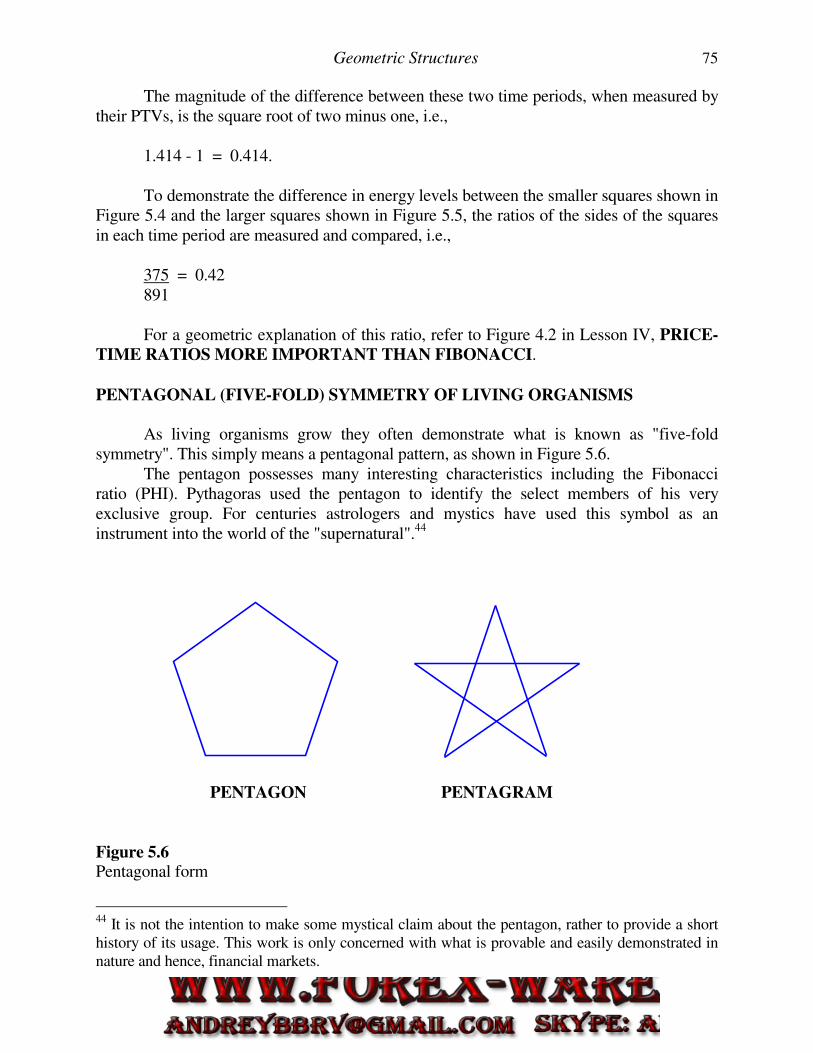
Geometric Structures 75
The magnitude of the difference between these two time periods, when measured by their PTVs, is the square root of two minus one, i.e., 1.414 - 1 = 0.414. To demonstrate the difference in energy levels between the smaller squares shown in Figure 5.4 and the larger squares shown in Figure 5.5, the ratios of the sides of the squares in each time period are measured and compared, i.e., 375 = 0.42 891 For a geometric explanation of this ratio, refer to Figure 4.2 in Lesson IV, PRICE-
TIME RATIOS MORE IMPORTANT THAN FIBONACCI.
PENTAGONAL (FIVE-FOLD) SYMMETRY OF LIVING ORGANISMS
As living organisms grow they often demonstrate what is known as "five-fold symmetry". This simply means a pentagonal pattern, as shown in Figure 5.6. The pentagon possesses many interesting characteristics including the Fibonacci ratio (PHI). Pythagoras used the pentagon to identify the select members of his very exclusive group. For centuries astrologers and mystics have used this symbol as an instrument into the world of the "supernatural".44
PENTAGON PENTAGRAM
Figure 5.6 Pentagonal form
44 It is not the intention to make some mystical claim about the pentagon, rather to provide a short history of its usage. This work is only concerned with what is provable and easily demonstrated in nature and hence, financial markets.
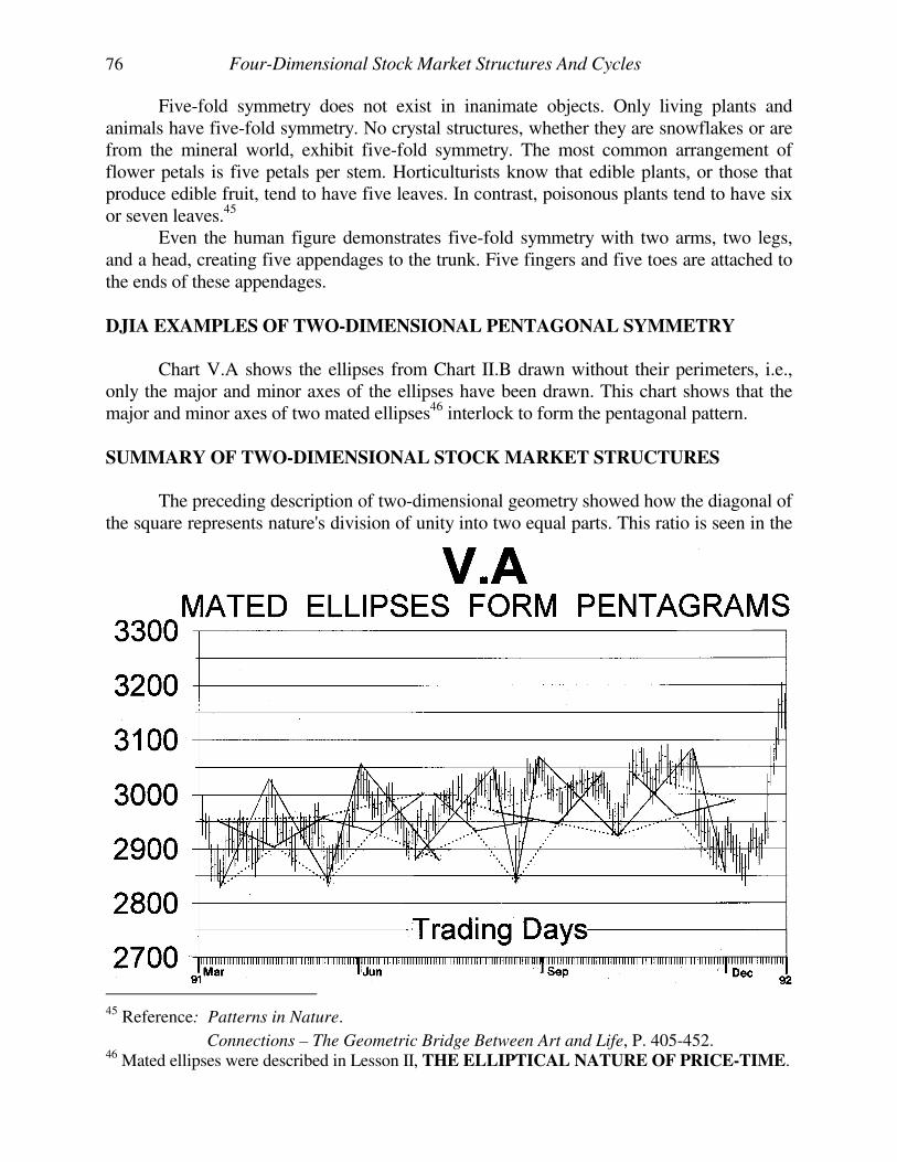
76 Four-Dimensional Stock Market Structures And Cycles
Five-fold symmetry does not exist in inanimate objects. Only living plants and animals have five-fold symmetry. No crystal structures, whether they are snowflakes or are from the mineral world, exhibit five-fold symmetry. The most common arrangement of flower petals is five petals per stem. Horticulturists know that edible plants, or those that produce edible fruit, tend to have five leaves. In contrast, poisonous plants tend to have six or seven leaves.45 Even the human figure demonstrates five-fold symmetry with two arms, two legs, and a head, creating five appendages to the trunk. Five fingers and five toes are attached to the ends of these appendages.
DJIA EXAMPLES OF TWO-DIMENSIONAL PENTAGONAL SYMMETRY
Chart V.A shows the ellipses from Chart II.B drawn without their perimeters, i.e., only the major and minor axes of the ellipses have been drawn. This chart shows that the major and minor axes of two mated ellipses46 interlock to form the pentagonal pattern.
SUMMARY OF TWO-DIMENSIONAL STOCK MARKET STRUCTURES
The preceding description of two-dimensional geometry showed how the diagonal of the square represents nature's division of unity into two equal parts. This ratio is seen in the
45 Reference: Patterns in Nature.
Connections – The Geometric Bridge Between Art and Life, P. 405-452. 46 Mated ellipses were described in Lesson II, THE ELLIPTICAL NATURE OF PRICE-TIME.
Geometric Structures 77
sequence of squares developing in the stock market, depending upon whether the square is crossed laterally or diagonally. Relationships were shown identifying certain PTVs as either the side of a square, the diagonal of a square, or the diagonal of two adjacent squares. The actual values calculated from the historic data had less than one percent error when compared to the ideal theoretical values. In the next section the arrangement of these squares will be shown to clearly form three-dimensional structures as seen on two-dimensional price-time charts.
THREE-DIMENSIONAL GEOMETRY
To this point this lesson has only addressed two-dimensional geometry. Two-dimensional analysis is useful when looking at a single face of the geometric solid at a time. However, a three-dimensional perspective is required to understand the anomalies encountered in price-time when the two-dimensional face of the structure completes its growth process and the structure rotates to expose the new face. This section provides the tools for a three-dimensional analysis of price-time geometry.
Traditional two-dimensional price-time charts of financial markets do not accurately represent the motion. This limitation of two-dimensional charts results in the appearance of price-time twisting into and turn out of the page of observation. However, as will be explained in Lesson X, DIMENSIONAL ASPECTS OF TIME, the price-time action is actually moving through man's three-dimensional perception, and man takes that three-dimensional perception and further reduces it to a two-dimensional price-time chart. Further complicating the analysis, the element of time is not linear, as represented on traditional price-time charts. Albert Einstein proved this fact. Figure 5.3 showed a two-dimensional representation of the successive decrease in PTV length, and the squares containing them, during the decomposition period from 1966 to 1982. The three-dimensional counterpart of Figure 5.3 is shown in Figure 5.7. To help visualize the true construct present in this figure the squares are enclosed in circles, revealing a three-dimensional view of a conical helix. Compare Figure 5.7 with the conical helix shown in Figure 3.1. With knowledge of the underlying conic helix, the three-dimensional properties of Chart IV.A can be seen. The square represented by FG is the smaller square in Figure 5.7, while the larger square in Figure 5.7 is represented by EG. The reader should review Chart IV.A, while conceptualizing the true conical structure shown in Figure 5.7.47
47 Technical Reference: The exponential decay of an RL circuit is mathematically similar to
PTV decomposition. Engineering Circuit Analysis, P. 176, Modern Control Systems, P. 177-
178. The circular fields shown in Figure 5.7 are the magnetic movement of a spinning particle,
Introduction to Physics for Scientists and Engineers, P. 516.
Also reference, Fundamentals of Physics – Extended, P. 440-441;
Geometry of Art and Life, P. 124-141.
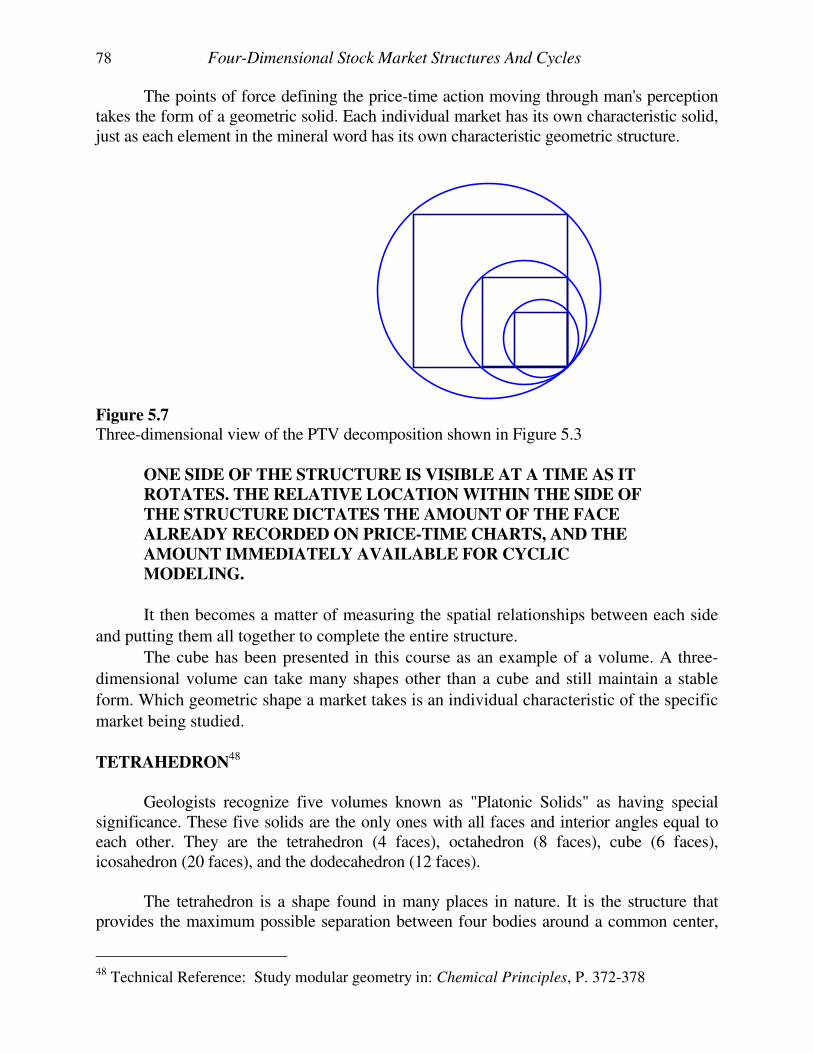
78 Four-Dimensional Stock Market Structures And Cycles
The points of force defining the price-time action moving through man's perception takes the form of a geometric solid. Each individual market has its own characteristic solid, just as each element in the mineral word has its own characteristic geometric structure.
Figure 5.7 Three-dimensional view of the PTV decomposition shown in Figure 5.3
ONE SIDE OF THE STRUCTURE IS VISIBLE AT A TIME AS IT
ROTATES. THE RELATIVE LOCATION WITHIN THE SIDE OF
THE STRUCTURE DICTATES THE AMOUNT OF THE FACE
ALREADY RECORDED ON PRICE-TIME CHARTS, AND THE
AMOUNT IMMEDIATELY AVAILABLE FOR CYCLIC
MODELING.
It then becomes a matter of measuring the spatial relationships between each side
and putting them all together to complete the entire structure.
The cube has been presented in this course as an example of a volume. A three-
dimensional volume can take many shapes other than a cube and still maintain a stable
form. Which geometric shape a market takes is an individual characteristic of the specific
market being studied.
TETRAHEDRON
48
Geologists recognize five volumes known as "Platonic Solids" as having special significance. These five solids are the only ones with all faces and interior angles equal to each other. They are the tetrahedron (4 faces), octahedron (8 faces), cube (6 faces), icosahedron (20 faces), and the dodecahedron (12 faces). The tetrahedron is a shape found in many places in nature. It is the structure that provides the maximum possible separation between four bodies around a common center,
48 Technical Reference: Study modular geometry in: Chemical Principles, P. 372-378
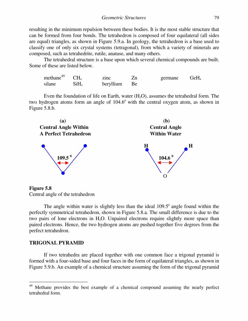
Geometric Structures 79
resulting in the minimum repulsion between these bodies. It is the most stable structure that can be formed from four bonds. The tetrahedron is composed of four equilateral (all sides are equal) triangles, as shown in Figure 5.9.a. In geology, the tetrahedron is a base used to classify one of only six crystal systems (tetragonal), from which a variety of minerals are composed, such as tetrahedrite, rutile, anatase, and many others. The tetrahedral structure is a base upon which several chemical compounds are built. Some of these are listed below. methane49 CH4 zinc Zn germane GeH4 silane SiH4 beryllium Be
Even the foundation of life on Earth, water (H2O), assumes the tetrahedral form. The two hydrogen atoms form an angle of 104.60 with the central oxygen atom, as shown in Figure 5.8.b.
(a) (b)
Central Angle Within Central Angle
A Perfect Tetrahedron Within Water
H H
109.5 0 104.6
0
O Figure 5.8
Central angle of the tetrahedron
The angle within water is slightly less than the ideal 109.50 angle found within the perfectly symmetrical tetrahedron, shown in Figure 5.8.a. The small difference is due to the two pairs of lone electrons in H2O. Unpaired electrons require slightly more space than paired electrons. Hence, the two hydrogen atoms are pushed together five degrees from the perfect tetrahedron.
TRIGONAL PYRAMID
If two tetrahedra are placed together with one common face a trigonal pyramid is formed with a four-sided base and four faces in the form of equilateral triangles, as shown in Figure 5.9.b. An example of a chemical structure assuming the form of the trigonal pyramid
49 Methane provides the best example of a chemical compound assuming the nearly perfect tetrahedral form.
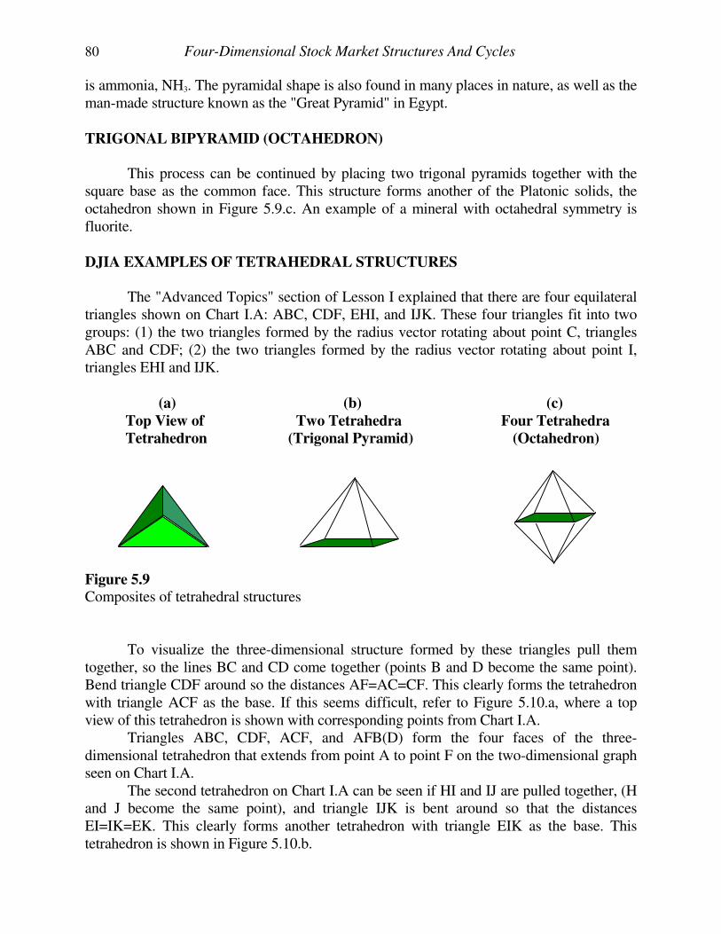
80 Four-Dimensional Stock Market Structures And Cycles
is ammonia, NH3. The pyramidal shape is also found in many places in nature, as well as the man-made structure known as the "Great Pyramid" in Egypt.
TRIGONAL BIPYRAMID (OCTAHEDRON)
This process can be continued by placing two trigonal pyramids together with the square base as the common face. This structure forms another of the Platonic solids, the octahedron shown in Figure 5.9.c. An example of a mineral with octahedral symmetry is fluorite.
DJIA EXAMPLES OF TETRAHEDRAL STRUCTURES
The "Advanced Topics" section of Lesson I explained that there are four equilateral triangles shown on Chart I.A: ABC, CDF, EHI, and IJK. These four triangles fit into two groups: (1) the two triangles formed by the radius vector rotating about point C, triangles ABC and CDF; (2) the two triangles formed by the radius vector rotating about point I, triangles EHI and IJK.
(a) (b) (c)
Top View of Two Tetrahedra Four Tetrahedra
Tetrahedron (Trigonal Pyramid) (Octahedron)
Figure 5.9
Composites of tetrahedral structures
To visualize the three-dimensional structure formed by these triangles pull them together, so the lines BC and CD come together (points B and D become the same point). Bend triangle CDF around so the distances AF=AC=CF. This clearly forms the tetrahedron with triangle ACF as the base. If this seems difficult, refer to Figure 5.10.a, where a top view of this tetrahedron is shown with corresponding points from Chart I.A. Triangles ABC, CDF, ACF, and AFB(D) form the four faces of the three-dimensional tetrahedron that extends from point A to point F on the two-dimensional graph seen on Chart I.A. The second tetrahedron on Chart I.A can be seen if HI and IJ are pulled together, (H and J become the same point), and triangle IJK is bent around so that the distances EI=IK=EK. This clearly forms another tetrahedron with triangle EIK as the base. This tetrahedron is shown in Figure 5.10.b.
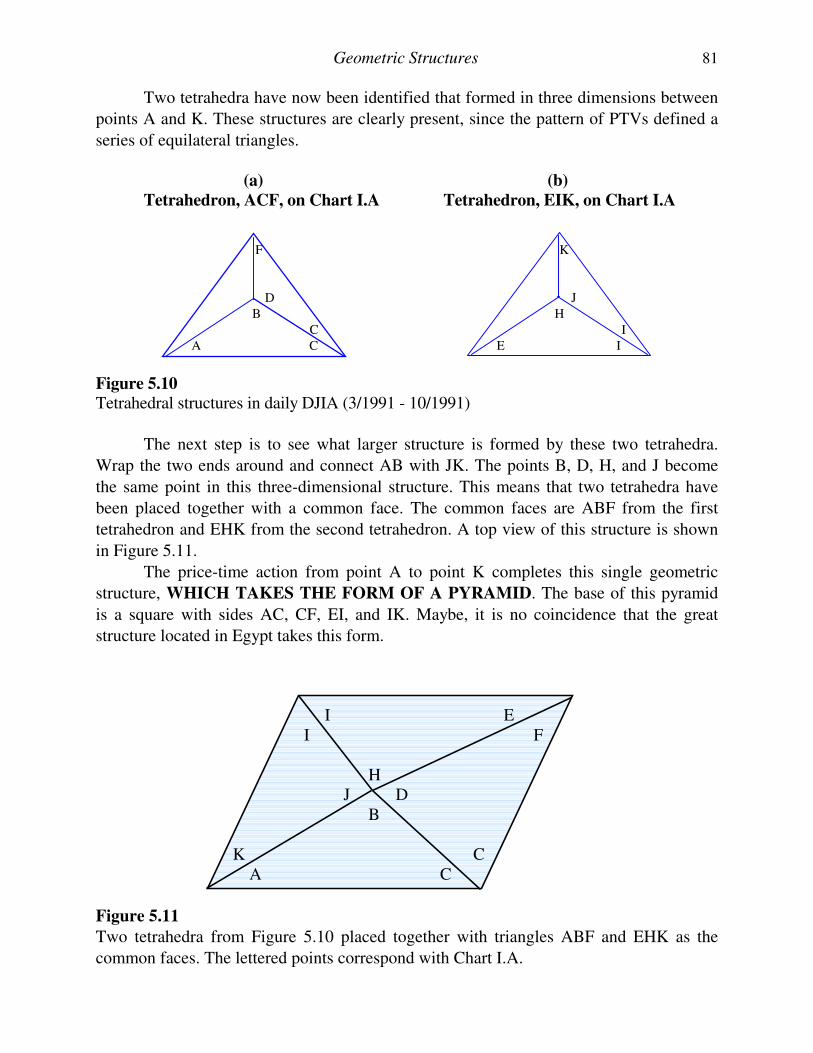
Geometric Structures 81
Two tetrahedra have now been identified that formed in three dimensions between
points A and K. These structures are clearly present, since the pattern of PTVs defined a
series of equilateral triangles.
(a) (b)
Tetrahedron, ACF, on Chart I.A Tetrahedron, EIK, on Chart I.A
F K
D J
B H
C I
A C E I
Figure 5.10
Tetrahedral structures in daily DJIA (3/1991 - 10/1991)
The next step is to see what larger structure is formed by these two tetrahedra.
Wrap the two ends around and connect AB with JK. The points B, D, H, and J become
the same point in this three-dimensional structure. This means that two tetrahedra have
been placed together with a common face. The common faces are ABF from the first
tetrahedron and EHK from the second tetrahedron. A top view of this structure is shown
in Figure 5.11.
The price-time action from point A to point K completes this single geometric
structure, WHICH TAKES THE FORM OF A PYRAMID. The base of this pyramid
is a square with sides AC, CF, EI, and IK. Maybe, it is no coincidence that the great
structure located in Egypt takes this form. I E I F H J D B K C A C
Figure 5.11
Two tetrahedra from Figure 5.10 placed together with triangles ABF and EHK as the
common faces. The lettered points correspond with Chart I.A.
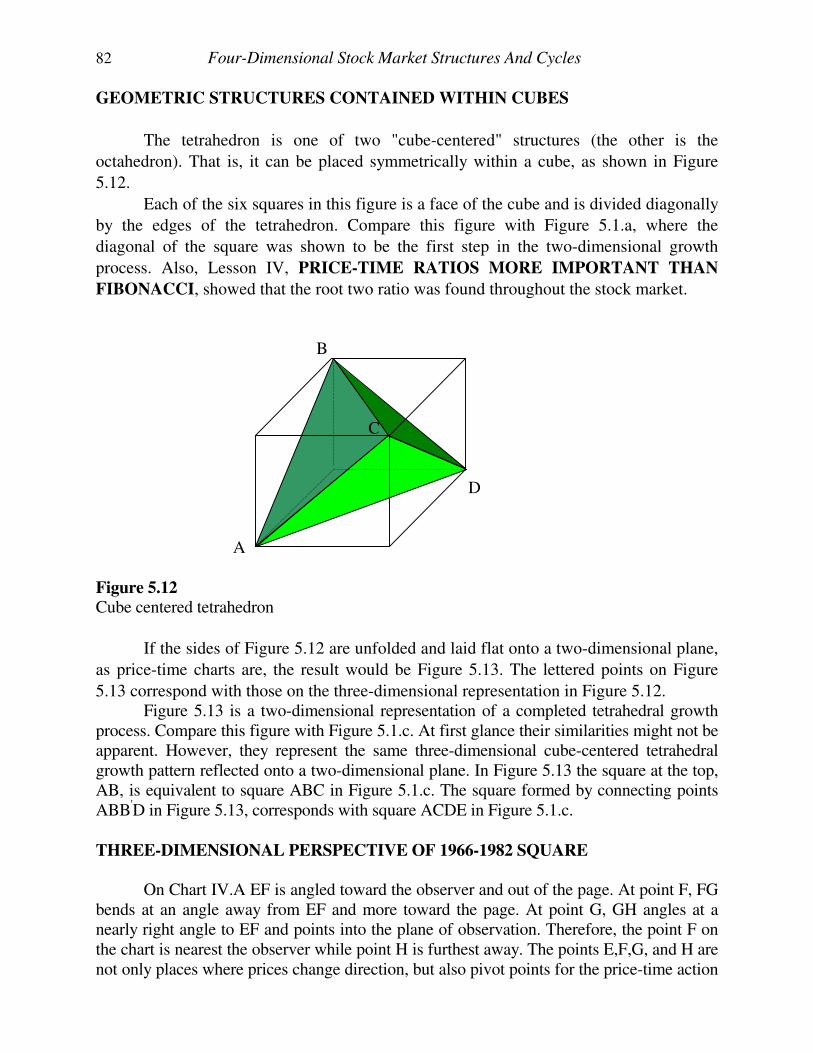
82 Four-Dimensional Stock Market Structures And Cycles
GEOMETRIC STRUCTURES CONTAINED WITHIN CUBES
The tetrahedron is one of two "cube-centered" structures (the other is the
octahedron). That is, it can be placed symmetrically within a cube, as shown in Figure
5.12.
Each of the six squares in this figure is a face of the cube and is divided diagonally
by the edges of the tetrahedron. Compare this figure with Figure 5.1.a, where the
diagonal of the square was shown to be the first step in the two-dimensional growth
process. Also, Lesson IV, PRICE-TIME RATIOS MORE IMPORTANT THAN
FIBONACCI, showed that the root two ratio was found throughout the stock market.
B
C
D
A
Figure 5.12
Cube centered tetrahedron
If the sides of Figure 5.12 are unfolded and laid flat onto a two-dimensional plane,
as price-time charts are, the result would be Figure 5.13. The lettered points on Figure
5.13 correspond with those on the three-dimensional representation in Figure 5.12. Figure 5.13 is a two-dimensional representation of a completed tetrahedral growth process. Compare this figure with Figure 5.1.c. At first glance their similarities might not be apparent. However, they represent the same three-dimensional cube-centered tetrahedral growth pattern reflected onto a two-dimensional plane. In Figure 5.13 the square at the top, AB, is equivalent to square ABC in Figure 5.1.c. The square formed by connecting points ABB'D in Figure 5.13, corresponds with square ACDE in Figure 5.1.c. THREE-DIMENSIONAL PERSPECTIVE OF 1966-1982 SQUARE
On Chart IV.A EF is angled toward the observer and out of the page. At point F, FG bends at an angle away from EF and more toward the page. At point G, GH angles at a nearly right angle to EF and points into the plane of observation. Therefore, the point F on the chart is nearest the observer while point H is furthest away. The points E,F,G, and H are not only places where prices change direction, but also pivot points for the price-time action
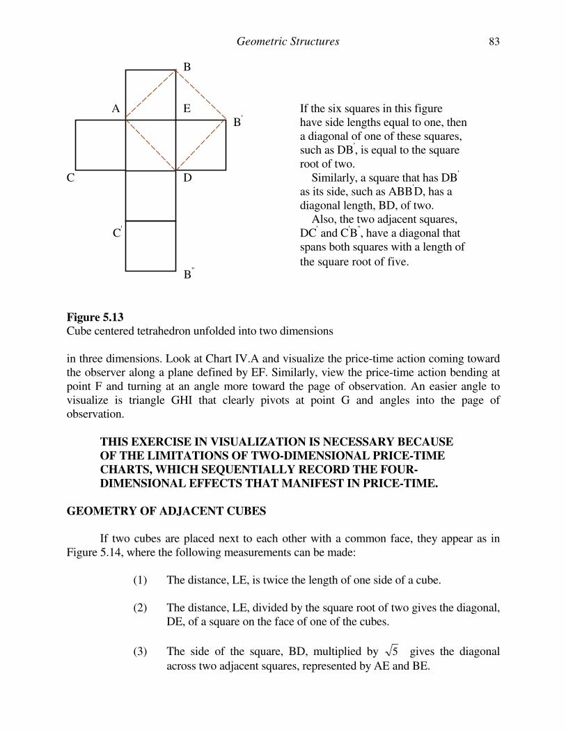
Geometric Structures 83
B A E B'
C D C'
B''
If the six squares in this figure have side lengths equal to one, then a diagonal of one of these squares, such as DB', is equal to the square root of two. Similarly, a square that has DB' as its side, such as ABB'D, has a diagonal length, BD, of two. Also, the two adjacent squares, DC' and C'B'', have a diagonal that spans both squares with a length of
the square root of five.
Figure 5.13
Cube centered tetrahedron unfolded into two dimensions
in three dimensions. Look at Chart IV.A and visualize the price-time action coming toward the observer along a plane defined by EF. Similarly, view the price-time action bending at point F and turning at an angle more toward the page of observation. An easier angle to visualize is triangle GHI that clearly pivots at point G and angles into the page of observation.
THIS EXERCISE IN VISUALIZATION IS NECESSARY BECAUSE
OF THE LIMITATIONS OF TWO-DIMENSIONAL PRICE-TIME
CHARTS, WHICH SEQUENTIALLY RECORD THE FOUR-
DIMENSIONAL EFFECTS THAT MANIFEST IN PRICE-TIME.
GEOMETRY OF ADJACENT CUBES
If two cubes are placed next to each other with a common face, they appear as in Figure 5.14, where the following measurements can be made: (1) The distance, LE, is twice the length of one side of a cube. (2) The distance, LE, divided by the square root of two gives the diagonal,
DE, of a square on the face of one of the cubes.
(3) The side of the square, BD, multiplied by 5 gives the diagonal
across two adjacent squares, represented by AE and BE.
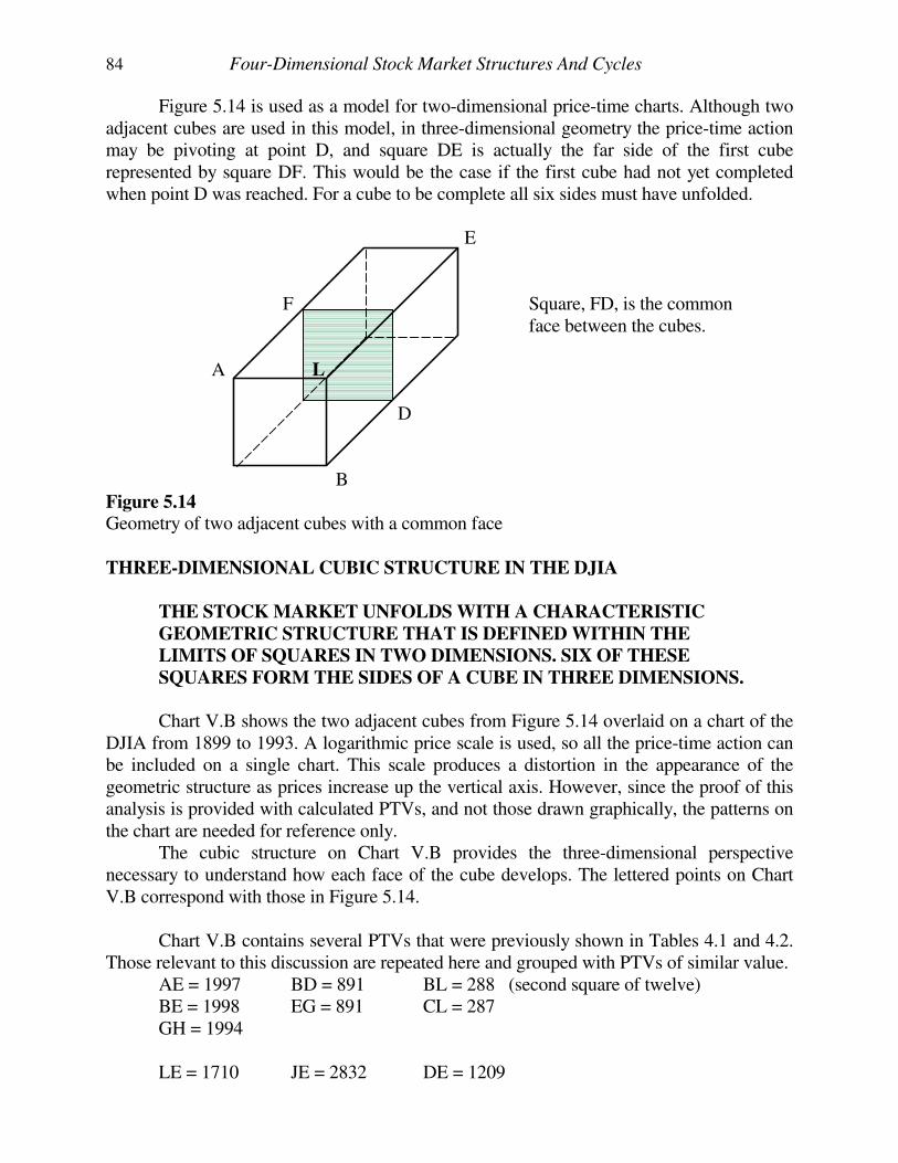
84 Four-Dimensional Stock Market Structures And Cycles
Figure 5.14 is used as a model for two-dimensional price-time charts. Although two adjacent cubes are used in this model, in three-dimensional geometry the price-time action may be pivoting at point D, and square DE is actually the far side of the first cube represented by square DF. This would be the case if the first cube had not yet completed when point D was reached. For a cube to be complete all six sides must have unfolded. E F Square, FD, is the common face between the cubes. A L D B Figure 5.14
Geometry of two adjacent cubes with a common face
THREE-DIMENSIONAL CUBIC STRUCTURE IN THE DJIA
THE STOCK MARKET UNFOLDS WITH A CHARACTERISTIC
GEOMETRIC STRUCTURE THAT IS DEFINED WITHIN THE
LIMITS OF SQUARES IN TWO DIMENSIONS. SIX OF THESE
SQUARES FORM THE SIDES OF A CUBE IN THREE DIMENSIONS.
Chart V.B shows the two adjacent cubes from Figure 5.14 overlaid on a chart of the DJIA from 1899 to 1993. A logarithmic price scale is used, so all the price-time action can be included on a single chart. This scale produces a distortion in the appearance of the geometric structure as prices increase up the vertical axis. However, since the proof of this analysis is provided with calculated PTVs, and not those drawn graphically, the patterns on the chart are needed for reference only. The cubic structure on Chart V.B provides the three-dimensional perspective necessary to understand how each face of the cube develops. The lettered points on Chart V.B correspond with those in Figure 5.14. Chart V.B contains several PTVs that were previously shown in Tables 4.1 and 4.2. Those relevant to this discussion are repeated here and grouped with PTVs of similar value. AE = 1997 BD = 891 BL = 288 (second square of twelve) BE = 1998 EG = 891 CL = 287 GH = 1994 LE = 1710 JE = 2832 DE = 1209
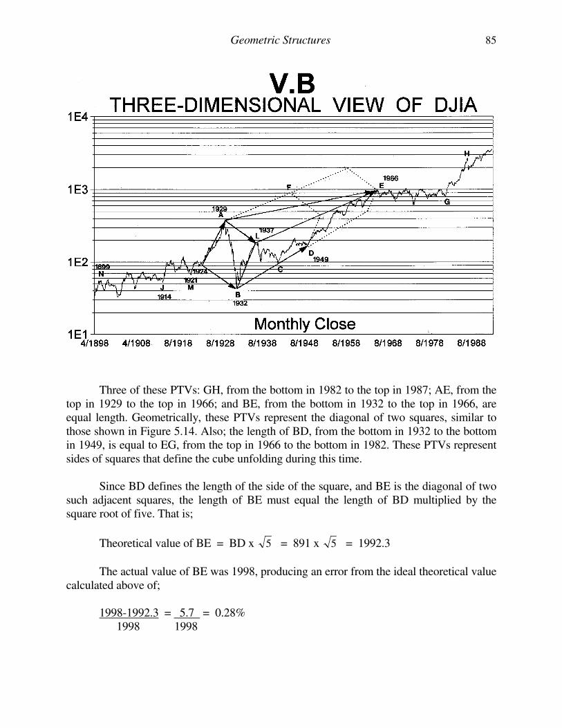
Geometric Structures 85
Three of these PTVs: GH, from the bottom in 1982 to the top in 1987; AE, from the top in 1929 to the top in 1966; and BE, from the bottom in 1932 to the top in 1966, are equal length. Geometrically, these PTVs represent the diagonal of two squares, similar to those shown in Figure 5.14. Also; the length of BD, from the bottom in 1932 to the bottom in 1949, is equal to EG, from the top in 1966 to the bottom in 1982. These PTVs represent sides of squares that define the cube unfolding during this time. Since BD defines the length of the side of the square, and BE is the diagonal of two such adjacent squares, the length of BE must equal the length of BD multiplied by the square root of five. That is;
Theoretical value of BE = BD x 5 = 891 x 5 = 1992.3
The actual value of BE was 1998, producing an error from the ideal theoretical value calculated above of; 1998-1992.3 = 5.7 = 0.28% 1998 1998
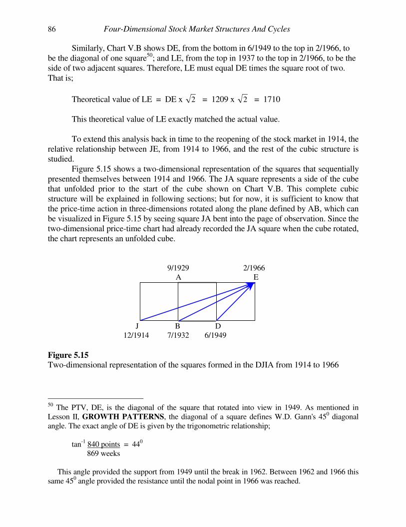
86 Four-Dimensional Stock Market Structures And Cycles
Similarly, Chart V.B shows DE, from the bottom in 6/1949 to the top in 2/1966, to be the diagonal of one square50; and LE, from the top in 1937 to the top in 2/1966, to be the side of two adjacent squares. Therefore, LE must equal DE times the square root of two. That is;
Theoretical value of LE = DE x 2 = 1209 x 2 = 1710 This theoretical value of LE exactly matched the actual value. To extend this analysis back in time to the reopening of the stock market in 1914, the relative relationship between JE, from 1914 to 1966, and the rest of the cubic structure is studied. Figure 5.15 shows a two-dimensional representation of the squares that sequentially presented themselves between 1914 and 1966. The JA square represents a side of the cube that unfolded prior to the start of the cube shown on Chart V.B. This complete cubic structure will be explained in following sections; but for now, it is sufficient to know that the price-time action in three-dimensions rotated along the plane defined by AB, which can be visualized in Figure 5.15 by seeing square JA bent into the page of observation. Since the two-dimensional price-time chart had already recorded the JA square when the cube rotated, the chart represents an unfolded cube. 9/1929 2/1966 A E J B D 12/1914 7/1932 6/1949
Figure 5.15 Two-dimensional representation of the squares formed in the DJIA from 1914 to 1966
50 The PTV, DE, is the diagonal of the square that rotated into view in 1949. As mentioned in Lesson II, GROWTH PATTERNS, the diagonal of a square defines W.D. Gann's 450 diagonal angle. The exact angle of DE is given by the trigonometric relationship; tan-1 840 points = 440 869 weeks This angle provided the support from 1949 until the break in 1962. Between 1962 and 1966 this same 450 angle provided the resistance until the nodal point in 1966 was reached.
Geometric Structures 87
BD is the length of the side of the large squares in Figure 5.15 and equals 891. Therefore, the length of JE is given by the square root of TEN times the side of the square, 891. That is;
Theoretical value of JE = BD x 10 = 891 x 10 = 2818
Table 4.2 showed the actual value of JE to be 2832, producing an error from the ideal theoretical value calculated above of; 2832 - 2818 = 14 = 0.49% 2832 2832
The relationship of the square root of ten has been previously explained as the square root of two multiplied by the square root of five. It also represents the diagonal of three adjacent squares. This relationship was shown in Figure 5.2.b between EF and the length of
the side of the smaller squares during that interval, (i.e., 200 x 10 = 632).
To further verify the relationship defined above between the squares in Figure 5.15, the ratio between JE and BE must be shown to be the square root of two. That is;
Theoretical value of JE = BE x 2 = 1998 x 2 = 2825.6 Since the actual value for JE was 2832, the error between the actual value and the ideal theoretical value calculated above is; 2832 - 2825.6 = 6.4 = 0.22% 2832 2832
SUMMARY OF THREE-DIMENSIONAL STOCK MARKET STRUCTURES
Figure 5.14 showed the three-dimensional characteristics of two cubes placed next to each other with a common face. This figure was overlaid on the price-time chart of the stock market to show the three-dimensional configuration between 1914 and 1966. The vectorial values (PTVs) were calculated between points on Chart V.B to show that the relative relationships between these PTVs were the same as for the sides of Figure 5.14. By calculating these PTVs and the ratios between them, it was shown that the price-time action on Chart V.B takes the three-dimensional form shown in Figure 5.14. Each of the ratios calculated in this section matched the ideal theoretical values within one percentage point! This is well within the reliability of the recorded data, and rules out the possibility of coincidence.
FOUR-DIMENSIONAL CUBIC STRUCTURES IN THE DJIA
While the three-dimensional perspective demonstrated in the previous section can
be seen on two-dimensional price-time charts, it does not accurately represent the true
88 Four-Dimensional Stock Market Structures And Cycles
configuration that is unfolding in price-time. The three-dimensional structure is visible
only because of the techniques used to record data on two-dimensional price-time charts.
To fully grasp the true nature of price-time, it must be understood that,
THE GEOMETRIC STRUCTURE DEFINING THE SPACIAL
RELATIONSHIP BETWEEN POINTS OF FORCE IN PRICE-TIME IS
IN MOTION RELATIVE TO THE DIMENSION OF MAN'S PERCEPTION.51
This initially may sound complicated. However, all it really means is that the geometric solid defining the long-term turning points in the stock market acts like a rotating cube. This appearance of rotation is caused by the twisting nature of the conical helix containing the structure. For example, the previous section showed two adjacent cubes overlaid on price-time between 1929 and 1966. However, THE ACTUAL GEOMETRIC STRUCTURE
THAT UNFOLDED BETWEEN 1899 AND 1982 WAS A SINGLE CUBE. The point on Figure 5.14 where it appears the price-time action was transferring from one cube to the next is actually the point in price-time where the cube rotated to expose its next face. This occurred in 1949. In four-dimensional reality, DE did not move to a different cube. Rather, it crossed the face of the cube that is represented by square DF. Remember, two-dimensional price-time charts only record data happening at that particular instant in time. The face of the geometric structure that lies in the future is hidden from view. In addition, the faces of the structure that have been previously recorded are unfolded onto a two-dimensional plane, as the data is recorded day-by-day. At first, the fact that the cube is rotating into view may create a source of confusion as two-dimensional charts are viewed, but this concept will become clearer when it is further explained in Lesson X, DIMENSIONAL ASPECTS OF TIME. As is the case with most new concepts, the more time spent studying the charts the clearer the concept will become. The conical helix expands as it grows. And since the faces of the cube are exposed as the conical helix twists, it follows that the squares defining these cubes also expand. This explains the increase in energy levels seen as time progresses. The growth process at any particular energy level is complete when the six sides of the cube have completed. After the cube completes, the growth proceeds to the next larger cube, which is stacked on top of the just completed cube. This effectively creates a formation similar to a pyramid with each succeeding cube larger than the previous one, as defined by the expanding conical helix. This was seen in 1949 when the smaller 1899-1949 cube completed and the energy level increased to complete the 1899-1982 cube, WHICH CONTAINED THE 1899-1949
CUBE. Therefore, the squares that defined the cube from 1899 to 1982 were larger than the squares that defined the 1899-1949 cube. Similarly, the squares from the 1899 to 1982 cube were smaller than the cube currently under construction (after the increase in energy level in 1982).
51 Technical Reference: Modern Physics, P. 20-23.
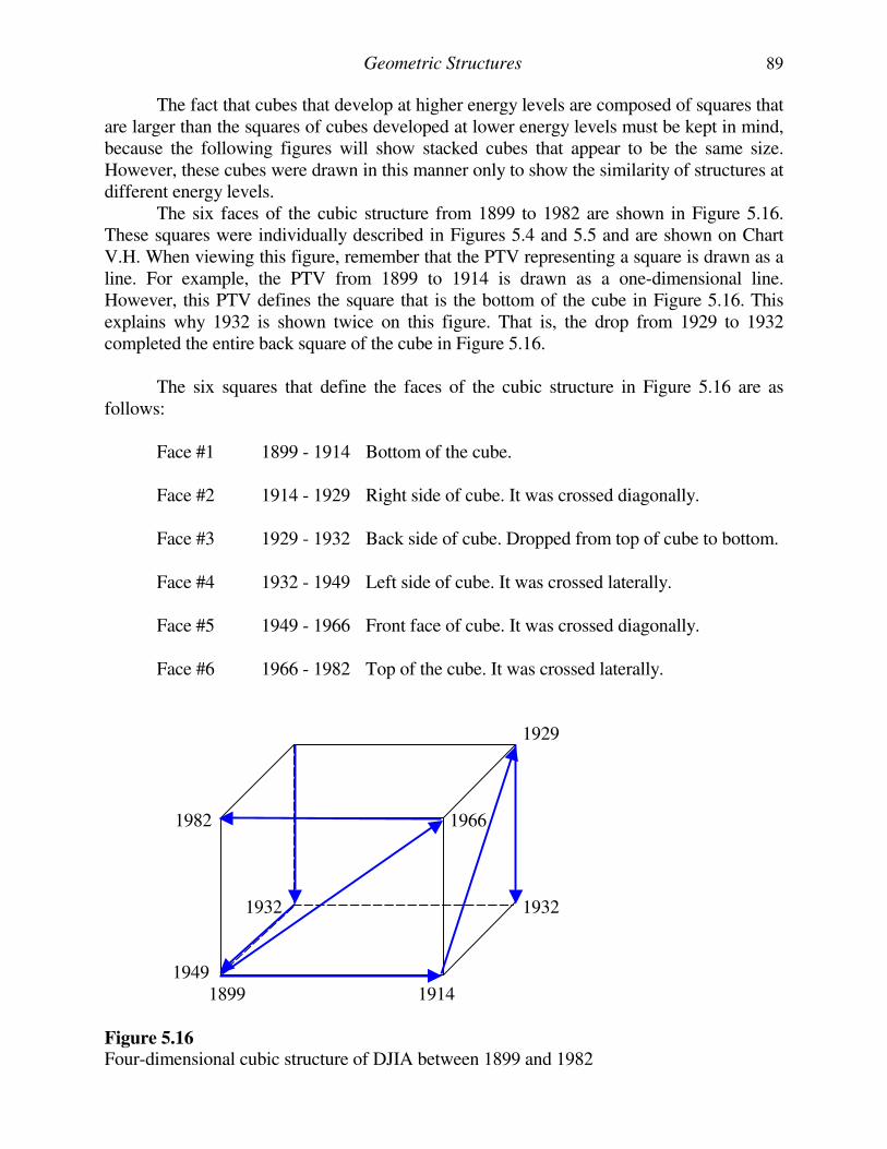
Geometric Structures 89
The fact that cubes that develop at higher energy levels are composed of squares that are larger than the squares of cubes developed at lower energy levels must be kept in mind, because the following figures will show stacked cubes that appear to be the same size. However, these cubes were drawn in this manner only to show the similarity of structures at different energy levels. The six faces of the cubic structure from 1899 to 1982 are shown in Figure 5.16. These squares were individually described in Figures 5.4 and 5.5 and are shown on Chart V.H. When viewing this figure, remember that the PTV representing a square is drawn as a line. For example, the PTV from 1899 to 1914 is drawn as a one-dimensional line. However, this PTV defines the square that is the bottom of the cube in Figure 5.16. This explains why 1932 is shown twice on this figure. That is, the drop from 1929 to 1932 completed the entire back square of the cube in Figure 5.16. The six squares that define the faces of the cubic structure in Figure 5.16 are as follows: Face #1 1899 - 1914 Bottom of the cube. Face #2 1914 - 1929 Right side of cube. It was crossed diagonally. Face #3 1929 - 1932 Back side of cube. Dropped from top of cube to bottom. Face #4 1932 - 1949 Left side of cube. It was crossed laterally. Face #5 1949 - 1966 Front face of cube. It was crossed diagonally. Face #6 1966 - 1982 Top of the cube. It was crossed laterally. 1929 1982 1966 1932 1932 1949 1899 1914
Figure 5.16 Four-dimensional cubic structure of DJIA between 1899 and 1982
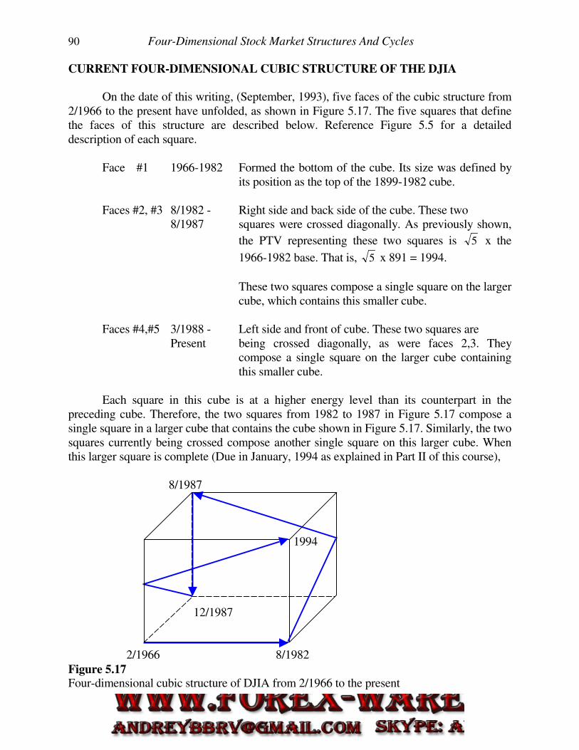
90 Four-Dimensional Stock Market Structures And Cycles
CURRENT FOUR-DIMENSIONAL CUBIC STRUCTURE OF THE DJIA
On the date of this writing, (September, 1993), five faces of the cubic structure from 2/1966 to the present have unfolded, as shown in Figure 5.17. The five squares that define the faces of this structure are described below. Reference Figure 5.5 for a detailed description of each square. Face #1 1966-1982 Formed the bottom of the cube. Its size was defined by
its position as the top of the 1899-1982 cube. Faces #2, #3 8/1982 - Right side and back side of the cube. These two 8/1987 squares were crossed diagonally. As previously shown,
the PTV representing these two squares is 5 x the
1966-1982 base. That is, 5 x 891 = 1994.
These two squares compose a single square on the larger
cube, which contains this smaller cube. Faces #4,#5 3/1988 - Left side and front of cube. These two squares are p Present being crossed diagonally, as were faces 2,3. They
compose a single square on the larger cube containing this smaller cube.
Each square in this cube is at a higher energy level than its counterpart in the preceding cube. Therefore, the two squares from 1982 to 1987 in Figure 5.17 compose a single square in a larger cube that contains the cube shown in Figure 5.17. Similarly, the two squares currently being crossed compose another single square on this larger cube. When this larger square is complete (Due in January, 1994 as explained in Part II of this course),
8/1987 1994 12/1987 2/1966 8/1982
Figure 5.17 Four-dimensional cubic structure of DJIA from 2/1966 to the present
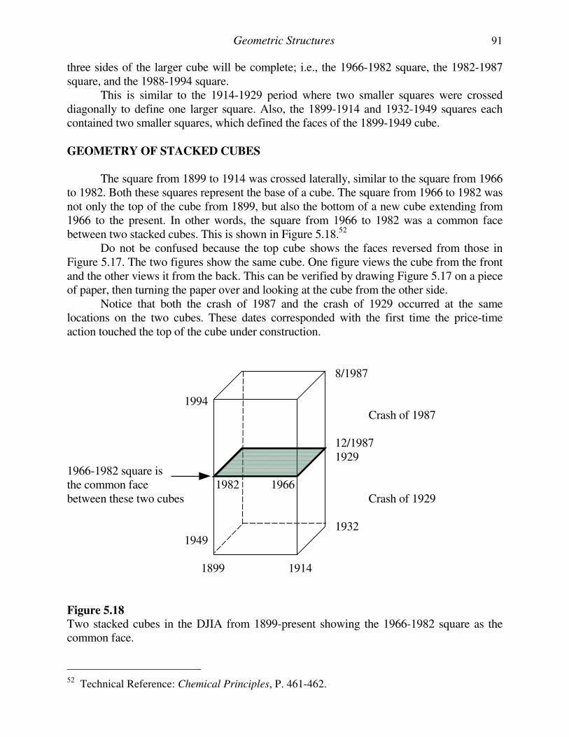
Geometric Structures 91
three sides of the larger cube will be complete; i.e., the 1966-1982 square, the 1982-1987 square, and the 1988-1994 square. This is similar to the 1914-1929 period where two smaller squares were crossed diagonally to define one larger square. Also, the 1899-1914 and 1932-1949 squares each contained two smaller squares, which defined the faces of the 1899-1949 cube. GEOMETRY OF STACKED CUBES
The square from 1899 to 1914 was crossed laterally, similar to the square from 1966 to 1982. Both these squares represent the base of a cube. The square from 1966 to 1982 was not only the top of the cube from 1899, but also the bottom of a new cube extending from 1966 to the present. In other words, the square from 1966 to 1982 was a common face between two stacked cubes. This is shown in Figure 5.18.52 Do not be confused because the top cube shows the faces reversed from those in Figure 5.17. The two figures show the same cube. One figure views the cube from the front and the other views it from the back. This can be verified by drawing Figure 5.17 on a piece of paper, then turning the paper over and looking at the cube from the other side. Notice that both the crash of 1987 and the crash of 1929 occurred at the same locations on the two cubes. These dates corresponded with the first time the price-time action touched the top of the cube under construction. 8/1987 1994 Crash of 1987 12/1987 1929 1966-1982 square is the common face 1982 1966 between these two cubes Crash of 1929 1932 1949 1899 1914
Figure 5.18
Two stacked cubes in the DJIA from 1899-present showing the 1966-1982 square as the common face.
52 Technical Reference: Chemical Principles, P. 461-462.
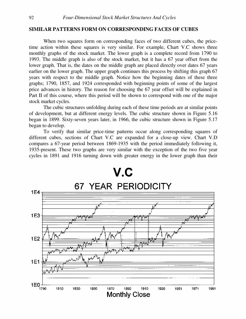
92 Four-Dimensional Stock Market Structures And Cycles
SIMILAR PATTERNS FORM ON CORRESPONDING FACES OF CUBES
When two squares form on corresponding faces of two different cubes, the price-time action within these squares is very similar. For example, Chart V.C shows three monthly graphs of the stock market. The lower graph is a complete record from 1790 to 1993. The middle graph is also of the stock market, but it has a 67 year offset from the lower graph. That is, the dates on the middle graph are placed directly over dates 67 years earlier on the lower graph. The upper graph continues this process by shifting this graph 67 years with respect to the middle graph. Notice how the beginning dates of these three graphs; 1790, 1857, and 1924 corresponded with beginning points of some of the largest price advances in history. The reason for choosing the 67 year offset will be explained in Part II of this course, where this period will be shown to correspond with one of the major stock market cycles. The cubic structures unfolding during each of these time periods are at similar points of development, but at different energy levels. The cubic structure shown in Figure 5.16 began in 1899. Sixty-seven years later, in 1966, the cubic structure shown in Figure 5.17 began to develop. To verify that similar price-time patterns occur along corresponding squares of different cubes, sections of Chart V.C are expanded for a close-up view. Chart V.D compares a 67-year period between 1869-1935 with the period immediately following it, 1935-present. These two graphs are very similar with the exception of the two five year cycles in 1891 and 1916 turning down with greater energy in the lower graph than their
Geometric Structures 93
corresponding cycles on the upper graph, i.e., 1958 and 1983. The location of the larger 84 year cycle explains why there was more energy in the 1958 and 1983 periods. This will be expanded in Lesson VIII.
Charts V.E and V.F provide a more detailed view of these corresponding sections
of the market, with twenty year periods graphed on the same chart. Chart V.E compares
the two periods between 1896-1915 and 1964-1983. Both these sections contain the
squares described in the previous section as bottoms of their respective cubes. Similarly,
they both represent tops of different cubes, as described in the section on stacked cubes.
In that section it was explained that the 1966-1982 square was the bottom of the cube
currently unfolding, and the top of the cube formed between 1899-1982.
The square between 1899-1914 was not only the bottom of the 1899-1982 cube, but
also, a common face shared with the cube formed prior to 1899.
Since the 1966-1982 square is the top of the cube originating in 1899, and the 1899-
1914 square is the bottom of the same cube, Chart V.E shows the top and bottom of this
same cube. Similarly, Chart V.F compares two twenty-year periods between 1870-1890 and
1935-1954.
The reader is encouraged to continue this process and compare the price-time
patterns on corresponding squares in different cubes. The long-term view is available on
Chart V.C.
CHAOS THEORY AND FRACTALS IN THE STOCK MARKET
This topic is scheduled to be included in future volumes of this course. Hence, only a brief overview will be provided. Chaos theory is the name given to a relatively new area of study in modern physics. The origin of Chaos theory was in 1961 when a scientist at MIT, Edward Lorenz, tried to create mathematical models to improve weather forecasting. The details of Chaos theory are available from many good books on the subject.53
An IBM scientist named Benoit Mandelbrot studied the specific area of Chaos theory
called FRACTALS. A fractal is a "fractioning" of a larger structure into smaller structures.
These smaller structures, fractals, have features similar to the larger structure. This theory
states that if a fractal is enlarged to the size of the larger structure the fractal will look like
the larger structure.
This theory should be nothing new for students of the Elliott Wave Theory, which
applies the 5-3 Elliott Wave pattern to financial market patterns of differing magnitude.
53 Reference: CHAOS.
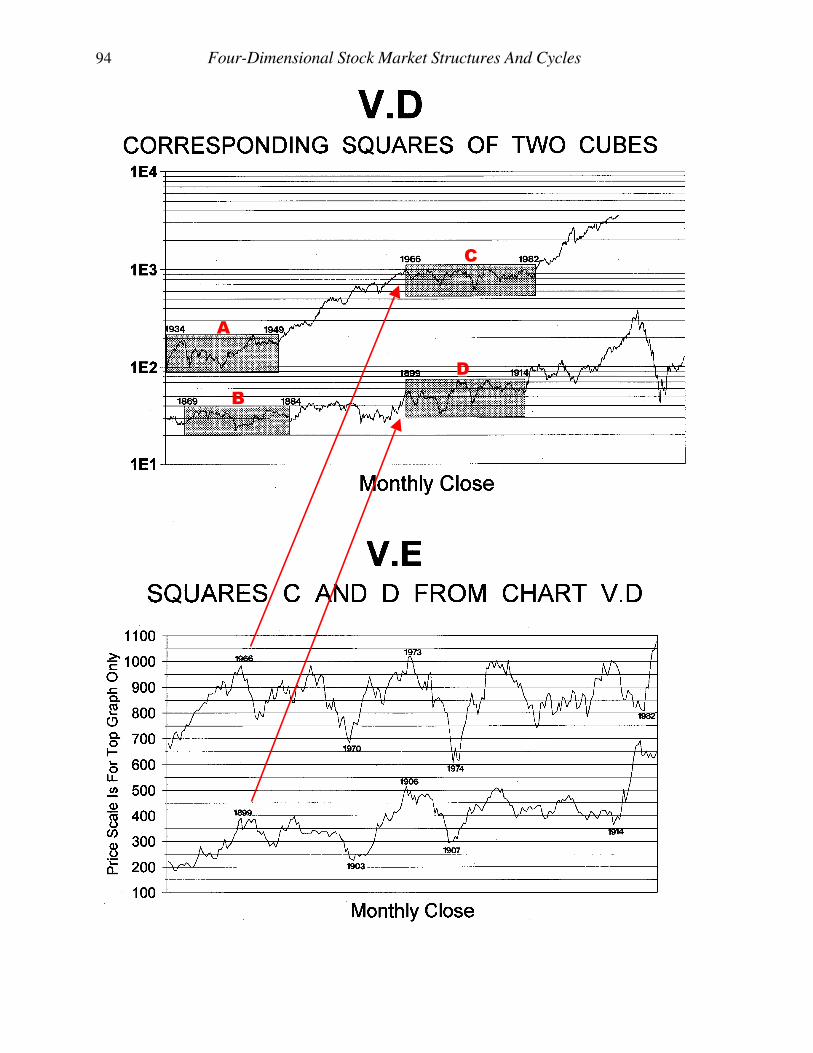
94 Four-Dimensional Stock Market Structures And Cycles
A
B
C
D
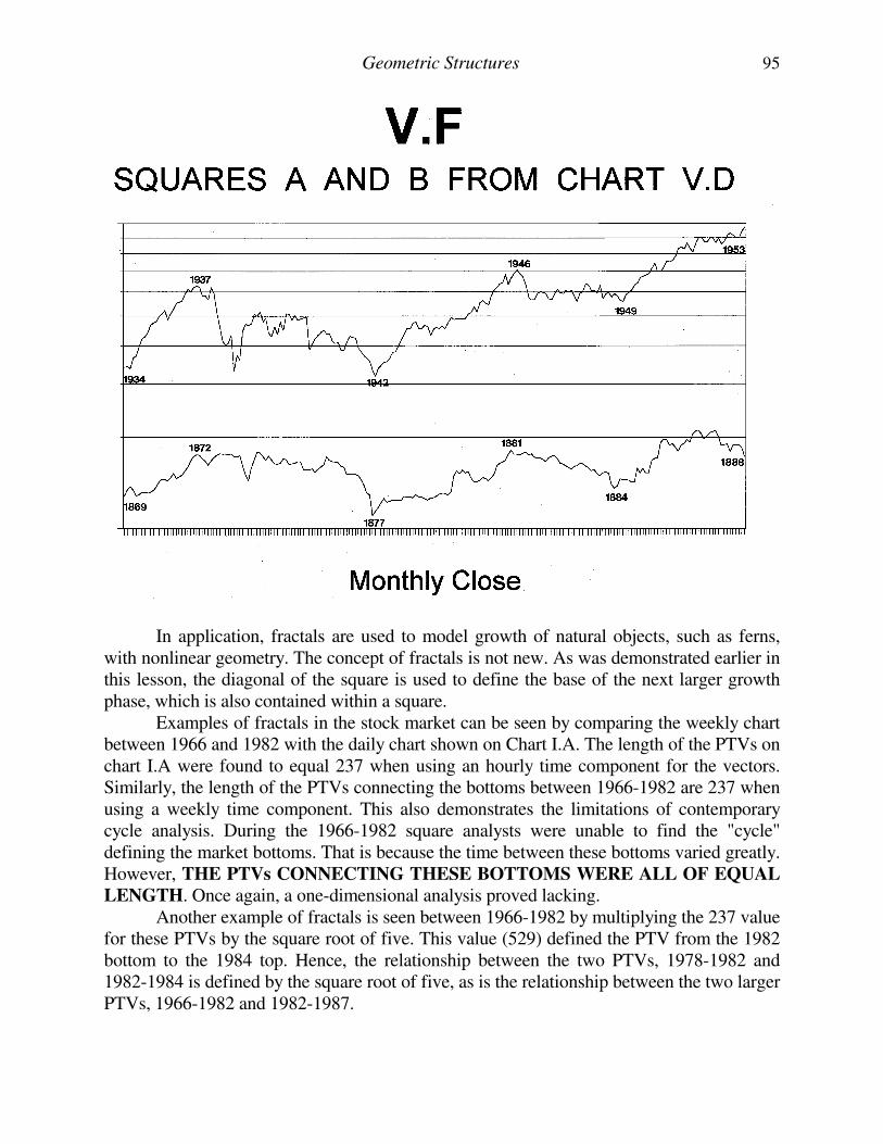
Geometric Structures 95
In application, fractals are used to model growth of natural objects, such as ferns, with nonlinear geometry. The concept of fractals is not new. As was demonstrated earlier in this lesson, the diagonal of the square is used to define the base of the next larger growth phase, which is also contained within a square. Examples of fractals in the stock market can be seen by comparing the weekly chart between 1966 and 1982 with the daily chart shown on Chart I.A. The length of the PTVs on chart I.A were found to equal 237 when using an hourly time component for the vectors. Similarly, the length of the PTVs connecting the bottoms between 1966-1982 are 237 when using a weekly time component. This also demonstrates the limitations of contemporary cycle analysis. During the 1966-1982 square analysts were unable to find the "cycle" defining the market bottoms. That is because the time between these bottoms varied greatly. However, THE PTVs CONNECTING THESE BOTTOMS WERE ALL OF EQUAL
LENGTH. Once again, a one-dimensional analysis proved lacking. Another example of fractals is seen between 1966-1982 by multiplying the 237 value for these PTVs by the square root of five. This value (529) defined the PTV from the 1982 bottom to the 1984 top. Hence, the relationship between the two PTVs, 1978-1982 and 1982-1984 is defined by the square root of five, as is the relationship between the two larger PTVs, 1966-1982 and 1982-1987.
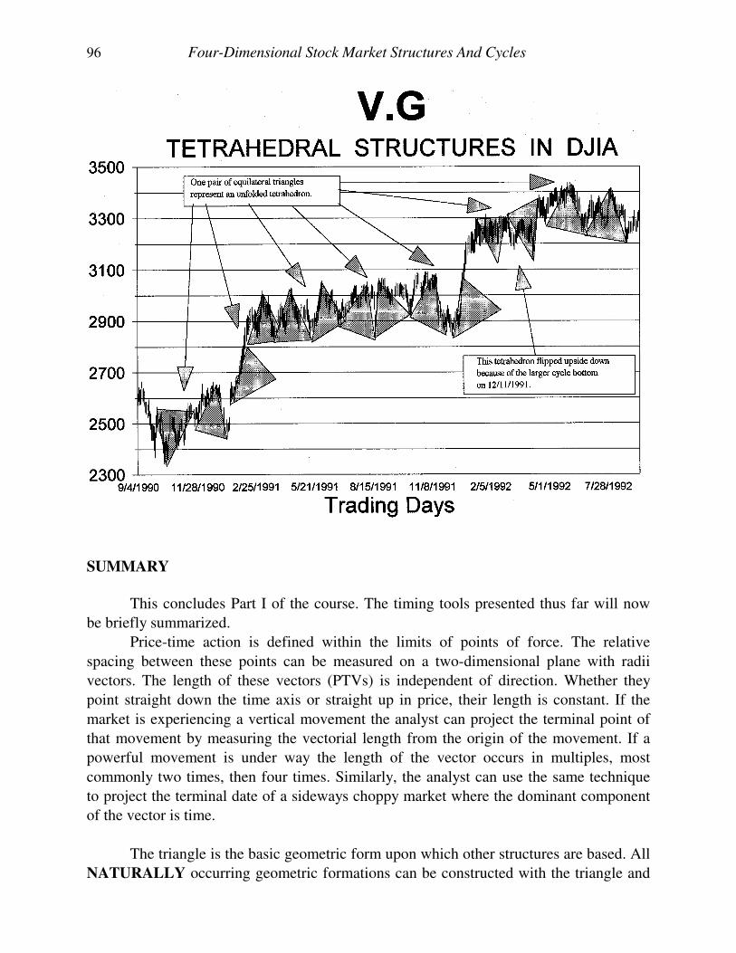
96 Four-Dimensional Stock Market Structures And Cycles
SUMMARY
This concludes Part I of the course. The timing tools presented thus far will now
be briefly summarized.
Price-time action is defined within the limits of points of force. The relative
spacing between these points can be measured on a two-dimensional plane with radii
vectors. The length of these vectors (PTVs) is independent of direction. Whether they
point straight down the time axis or straight up in price, their length is constant. If the
market is experiencing a vertical movement the analyst can project the terminal point of
that movement by measuring the vectorial length from the origin of the movement. If a
powerful movement is under way the length of the vector occurs in multiples, most
commonly two times, then four times. Similarly, the analyst can use the same technique
to project the terminal date of a sideways choppy market where the dominant component
of the vector is time.
The triangle is the basic geometric form upon which other structures are based. All
NATURALLY occurring geometric formations can be constructed with the triangle and
Geometric Structures 97
the circle. In the case of the stock market, two vectors interlock to create an equilateral
triangle. Therefore, the analyst not only knows in advance the length of the movement
under way, but also the direction of that movement, specifically 600 from its mated PTV.
Measurement of these equilateral triangles on a daily chart easily allows the analyst to
project terminal points of movements within two trading days.
The angle within water was shown to deviate from the ideal tetrahedral angle by
five degrees. The two pairs of lone electrons in water cause this deviation. This
phenomenon was explained because the DJIA experiences a similar shifting. If the angles
are measured within the triangles in the DJIA their exact value will be found to be
between 620 and 630. This two-degree difference within the faces of the DJIA triangles is
caused by the shifting within the inner angle of the three-dimensional tetrahedron.
In the case of the stock market, two equilateral triangles seen on a two-
dimensional price-time chart compose a three-dimensional tetrahedron. This tetrahedron
is unfolded as price-time charts sequentially record the faces as they present themselves.
If a market other that the stock market is studied, the composite formed will not
necessarily be tetrahedral. However, the triangle will still be the basic construct upon
which to build. Rather than the tetrahedral form, the composite may be an octahedron, a
dodecahedron, icosahedron, or some other form depending upon the specific lattice of
that market.
The tetrahedron is a "cube-centered" solid, meaning it can be placed
symmetrically within a cube. The cubic structure in the stock market between 1899 and
1982 was closely analyzed, and detailed measurements were made of each face of this
cube verifying its form.
Contained within this larger cube was the smaller cube extending from 1899 to
1949. This can be seen in Figure 5.19 where the smallest cube is the 1899-1949 cube.
Two sides of this smaller cube were found to complete one side of the larger cube. When
the smaller cube completed in 1949 the fourth side of the larger cube also completed. The
length of this fourth side, which extended from 1932 to 1949, was found to equal 891.
This value was the length of the top of the larger cube, which extended from 1966 to
1982. The four sides of the larger cube (1899-1982) were found to be progressively
increasing in size as the smaller cube unfolded. For example, the 1899-1914 square was
slightly smaller than the 1914-1929 square, which in turn was smaller than the 1932-1949
square. The increase in the side length of the larger cube was caused by the expanding
conical helix. It is the smaller cube (1899-1949) that is contained within the larger cube
that has constant side length. When the smaller cube completed in 1949 there was an
increase in energy levels as the fifth side of the larger cube was crossed diagonally to
reach its top.
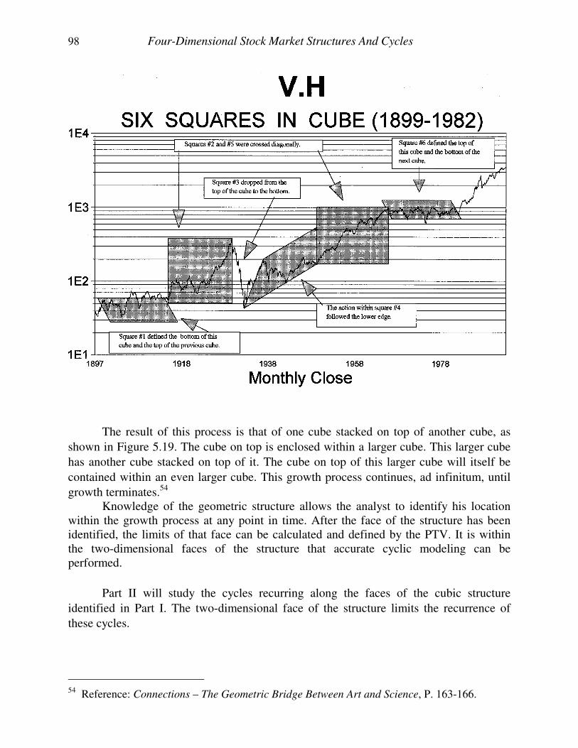
98 Four-Dimensional Stock Market Structures And Cycles
The result of this process is that of one cube stacked on top of another cube, as
shown in Figure 5.19. The cube on top is enclosed within a larger cube. This larger cube
has another cube stacked on top of it. The cube on top of this larger cube will itself be
contained within an even larger cube. This growth process continues, ad infinitum, until
growth terminates.54 Knowledge of the geometric structure allows the analyst to identify his location within the growth process at any point in time. After the face of the structure has been identified, the limits of that face can be calculated and defined by the PTV. It is within the two-dimensional faces of the structure that accurate cyclic modeling can be performed.
Part II will study the cycles recurring along the faces of the cubic structure
identified in Part I. The two-dimensional face of the structure limits the recurrence of
these cycles.
54 Reference: Connections – The Geometric Bridge Between Art and Science, P. 163-166.
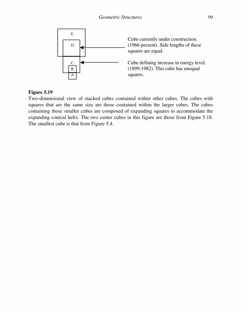
Geometric Structures 99
E
Cube currently under construction. D (1966-present). Side lengths of these squares are equal. C Cube defining increase in energy level. B (1899-1982). This cube has unequal A squares.
Figure 5.19
Two-dimensional view of stacked cubes contained within other cubes. The cubes with
squares that are the same size are those contained within the larger cubes. The cubes
containing these smaller cubes are composed of expanding squares to accommodate the
expanding conical helix. The two center cubes in this figure are those from Figure 5.18.
The smallest cube is that from Figure 5.4.

PART TWO
FOUR-DIMENSIONAL
PRICE-TIME CYCLES
INTRODUCTION
PART TWO
Part one of this course showed how to identify geometric structures in financial
markets. It was also shown that with application of the PTV, geometric ratios, and
knowledge of the cubic structure, the limits of the square can be determined years in
advance.
IT IS WITHIN THE LIMITS OF THE SQUARE THAT
CYCLES REPEAT WITH PREDICTABLE PERIODICITY.
When a new square begins the cycles within that square repeat with a periodicity
that usually differs from those in the preceding square. Therefore, the knowledge from
Part I of this course is critical if accurate cycle analysis is to be performed over any
extended period of time.
Traditional cycle analysts err in their approach by attempting to project cycles
beyond the limits of the square in which they are defined. As demonstrated in Part I,
when a square completes it rotates out of view.
Part II will show how the scientific phenomenon of "sympathetic resonance"
synchronizes cycles found in the stock market with the predictable periods of the planets
and their harmonics.
Tables will be used extensively in Part II, as they were in Part I, to provide the
data supporting all presented postulates. This data provides the indisputable proof of the
correlation between stock market cycles and planetary cycles. Numbers do not lie.
Do not be intimidated by tables filled with numbers. They simply record the
locations of the planets at different times in history. It is important the reader take the
time to review this data, for it is there and in the charts that the ultimate proof lies.
This course makes no claim that a cause-effect relationship exists between
planetary motion and stock market cycles. The data is simply gathered and displayed,
showing the correlation.
Volumes of material can be written describing the details of these cycles,
especially in the areas where double or triple tops or bottoms occur. These types of
formations occur when different cycles reach their tops or bottoms close to each other,
but not at exactly the same time. As more time is spent studying these multiple tops and
bottoms, more awareness of the truth of the theories presented in this course will be
gained.
If the reader has difficulty with the concept relating stock market cycles with
planetary cycles, the same results can be achieved by looking at the fifteen-degree axes of
elliptical cycles, which have the same periodicity as the planets. It is simply easier to use
the planets because of the availability of data.
LESSON VI
SYMPATHETIC RESONANCE
AND THE LAW OF VIBRATION
I have proven to myself, as well as demonstrated to others, that the Law of Vibration explains every possible phase and
condition of the market. ... W.D. Gann
INTRODUCTION
Sympathetic resonance is the scientific term for the natural phenomenon seen when a body is subjected to an external vibrating source with a frequency equal to that of the natural frequency of the body, the body itself begins to vibrate. For example, when two violin strings are in unison and one is bowed, the other will oscillate at the frequency of the bowed string. This will happen even though the second string is not touched by the bow. In order to explain this phenomenon, a brief explanation of simple vibration is necessary. Initially, it may be difficult to understand how this material relates to financial markets; however, EVERYTHING presented in the following explanation is directly applicable to financial markets. If the reader chooses to skip this explanation the material presented later will not make sense. The explanation is brief and broadly covers a variety of characteristics of this phenomenon. For those desiring more information on this subject, books of physics are available giving more detail. As previously stated, it is not the intention of the author to provide information available from other sources. Rather, the reader is referenced to those sources. A simple way to understand sympathetic resonance is to visualize a child swinging on a swing. If each time the swing returns someone gives the child another push, he will swing higher and higher. This is because the rate at which the swing is pushed equals the period of the swing. The two (the period of the swing and the act of pushing) are synchronous. Similarly, if the swing is pushed every other time it returns it will continue to swing. In this case, the swing and the push are synchronous with a ratio of two to one, i.e., two swings for one push. However, if the swing is pushed before it fully returns, the two will be out of phase and the swing will not swing higher. In this example the swing is the body being acted upon, the push is the external force, and the period of the swing is the natural frequency of the system.55
With respect to financial markets, sympathetic resonance allows an analyst to project, not only exactly where in price a market will advance or decline, but also WHEN it will happen. Time has always been the missing element in the projections of market analysts. However, TIME IS THE MOST IMPORTANT ELEMENT.
55 Technical References: Fundamentals of Physics – Extended. P. 387-390, 435-438.
Modern Control Systems, P. 145-146.
Sympathetic Resonance And The Law of Vibration 103
SYNCHRONICITY
Nature tends to synchronize elements that initially appear to be disharmonious. At times, achieving this synchronous state requires maximum entropy until a common denominator is obtained, after which, stability occurs. For example, when individual heart cells are removed from two living beating hearts, which are naturally beating at different rates, these two cells will continue to pulse at the rate of the heart from which they were removed. However, when these two cells are placed in contact with each other, both their rates of pulsation will change until a third beat different from either of the two original rates is attained. Both these cells will continue to beat at this third rate as long as oxygen and nutrients are supplied. They have synchronized with each other. Examples of this law abound in nature. Numerous researchers have found that when women are placed together for several hours each day their menstrual cycles synchronize. Even if the menstrual cycles are, initially, randomly distributed throughout the month, after a short period of time the cycles will synchronize.56 Synchrony even occurs with physical appearance. When people live together year after year they tend to start to look alike. Older couples not only attain similar mannerisms, but physically look more similar than they did when they met. These are all examples of natures force to synchronize. As with all natural laws, financial markets are not exempt from the phenomenon of synchronizing. In order to accurately time a financial market, it is simply a matter of finding with what other element in nature the particular market has synchronized, then determining if this other element provides predictability.
MUSICAL SCALES
Figure 6.1 shows strings of various lengths in a state of vibration. The string is used because it is the simplest example of a vibrating body. The fundamental tone is shown in 6.1.a, and the remaining tones (6.1.b through 6.1.f) are called "upper harmonics" to the fundamental tone.
The ratios between these tones (and the fundamental tone) define notes on the
musical "Diatonic Major Scale". For example, between 6.1.a and 6.1.b the ratio is two,
defining the octave. The ratio between 6.1.b and 6.1.c is three to two, defining the
musical fifth. The remaining ratios and their respective musical tones are shown on the
left side of the figure. On the right side of the figure is the ratio with respect to the
fundamental tone, 6.1.a.
Note that these musical intervals consist solely of octaves, fifths, and octaves of
fifths. This is the same system used by Pythagoras when he developed the "Diatonic
56 Reference: Nature, March 1998, Martha McClintock, University of Chicago. The entire menstrual cycle tends to synchronize. This includes the portion known as premenstrual syndrome (PMS). For those working in close proximity to numerous women who are simultaneously experiencing PMS where unpredictable mood swings can occur, this knowledge could be valuable.
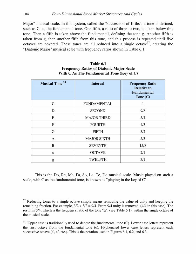
104 Four-Dimensional Stock Market Structures And Cycles
Major" musical scale. In this system, called the "succession of fifths", a tone is defined,
such as C, as the fundamental tone. One fifth, a ratio of three to two, is taken below this
tone. Then a fifth is taken above the fundamental, defining the tone g. Another fifth is
taken from g, then another fifth from this tone, and this process is repeated until five
octaves are covered. These tones are all reduced into a single octave57, creating the
"Diatonic Major" musical scale with frequency ratios shown in Table 6.1.
Table 6.1
Frequency Ratios of Diatonic Major Scale
With C As The Fundamental Tone (Key of C)
Musical Tone 58
Interval Frequency Ratio
Relative to
Fundamental
Tone (C)
C FUNDAMENTAL 1
D SECOND 9/8
E MAJOR THIRD 5/4
F FOURTH 4/3
G FIFTH 3/2
A MAJOR SIXTH 5/3
B SEVENTH 15/8
c OCTAVE 2/1
g TWELFTH 3/1
This is the Do, Re, Me, Fa, So, La, Te, Do musical scale. Music played on such a scale, with C as the fundamental tone, is known as "playing in the key of C".
57 Reducing tones to a single octave simply means removing the value of unity and keeping the remaining fraction. For example, 3/2 x 3/2 = 9/4. From 9/4 unity is removed, (4/4 in this case). The result is 5/4, which is the frequency ratio of the tone "E", (see Table 6.1), within the single octave of the musical scale.
58 Upper case is traditionally used to denote the fundamental tone (C). Lower case letters represent the first octave from the fundamental tone (c). Hyphenated lower case letters represent each successive octave (c', c'', etc.). This is the notation used in Figures 6.1, 6.2, and 6.3.
Sympathetic Resonance And The Law of Vibration 105
It is recommended the reader reference additional material concerning construction of the Diatonic Major Scale. This subject will not be further expanded here because this information is available from other sources. For the purpose of this discussion, remember that a sequence of "fifths" taken above a fundamental tone, and one below the fundamental, and all reduced to a single octave, define the "Diatonic Major" musical scale, as created by Pythagoras.
NODAL POINTS
Having achieved a basic understanding of the musical scale, attention can be focused on Figure 6.1. The lengths and hence, the frequency of the strings shown in this figure are successively divided by two ratios, the octave and the fifth.59 The points on this figure where the upper and lower lines come together are called NODES, and are places on the string where no motion occurs. For example, in 6.1.b there are two nodes at the end points and one node in the exact middle. Similarly, 6.1.c has two end nodes and two middle nodes, which divide the string into three equal vibrating lengths. The nodes are created as vibrations, which are sent through the string, bounce off the end points and interact with waves progressing in the opposite direction. At the points where nodes occur the waves add together to neutralize each other. The concept of nodes is very important because, as will be shown, financial markets also possess nodes, i.e., periods of little or no motion where cycles moving in different directions create trendless markets. Lesson IX, COMPOSITE CYCLES, expands the concept of nodes. To be in unison two strings do not have to be of equal length. Strings with lengths in the ratio of simple integers are also in unison. For example, the strings in Figure 6.1.a and 6.1.b are in unison with an integral ratio of two. Strings 6.1.b and 6.1.c are in unison with a ratio of the two integers three and two, and so on for the remaining lengths shown in the figure. Hence, a string is in unison with its harmonics.
If string 6.1.a (the fundamental tone) is set into vibration, string 6.1.b will also
begin to vibrate. Also, 6.1.c will vibrate, as will 6.1.d, 6.1.e, and so on. These strings are
in unison and will vibrate, sympathetically. Musicians are well aware of this
phenomenon, which causes the high-pitched "ringing" sound heard when the string of an
instrument is plucked. Without these "upper harmonics" the fundamental alone would
have a very dull sound.
It is very important to note THE STRING LENGTHS DO NOT HAVE TO BE
IN EXACT UNISON TO VIBRATE, SYMPATHETICALLY. If there is a minor
difference from the exact integral ratio the bodies will still resonate, sympathetically.
However, the further the bodies are from exact unison, the less sympathetic vibration will
occur. The importance of this will become apparent as the amount of sympathetic
resonance to expect in a financial market is determined given a certain amount of
variation from the ideal fundamental. This will be studied in Lesson VIII.
59 Technical Reference: Introduction to Physics for Scientists and Engineers. P. 581-584.
106 Four-Dimensional Stock Market Structures And Cycles
Rather than striking the fundamental tone shown in Figure 6.1.a, if the string in 6.1.b
is struck it will induce sympathetic vibration in its upper harmonics namely, 6.1.c, 6.1.d,
6.1.e, etc. However, the vibration that is sympathetically induced in 6.1.a will have less
magnitude than that in the upper harmonics. In other words, when a body is set into
vibration the upper harmonics (strings with shorter lengths) will vibrate, sympathetically,
with a much greater energy than the "lower harmonics" (strings with greater length than the
one set into motion).
This natural phenomenon is the scientific basis for the radio.60 A broadcasting station
plays a tape or compact disk into a transmitter, which sends out a signal in the form of
vibrations. These vibrations cause the circuitry inside the radio to vibrate, sympathetically,
recreating the signal that was broadcast.
From radio transmissions to the creation of the musical scale, examples of
sympathetic resonance can be found everywhere in nature. This is not limited to phenomena
occurring on Earth, but can also be seen in motions in the solar system. For example, THE
RELATIVE PERIODS OF THE PLANETS EXIST IN HARMONIC RATIOS,
IMPLYING SYMPATHETIC RESONANCE was at work on the stellar debris during
the formation process of the solar system.
Modern models of planetary formation have residue stellar debris originally
distributed evenly in a two-dimensional plane extending from the equator of the sun.
According to the theory, this material moved into areas where the least net force acted upon
it (nodal points). This migration of the stellar material effectively created areas with large
amounts of debris and areas with little or no debris. The areas where debris collected are
those where the planets formed. The areas where no debris was present were those with a
large net force acting on it, eventually moving the debris out of the area. The areas from
where the debris moved represent the spacing between the planets after the formation
process completed. The periods of the planets exist in harmonic ratios. This means the nodal points, which defined the areas in the stellar debris where the material collected and where the planets formed, divided into harmonic ratios.
This process is easily simulated in the laboratory by placing metal filings on a flat
sheet and subjecting the sheet to vibration. The metal filings move to areas where the
sheet vibrates the least, i.e., nodal points. If the vibration rate is changed the metal filings
move to another area on the sheet where the new nodes exist.
The harmonic ratios between the periods of the major planets are shown in Figure
6.2. This figure is the same as Figure 6.1, except the periods of the planets have been
inserted in the appropriate positions to show the harmonic relationships.
60 In 1909 W.D. Gann stated that his "Law of Vibration" was "the fundamental law upon which the wireless telegraphy, wireless telephones, and phonographs are based. Without the existence of (the Law of Vibration) the above inventions would have been impossible."
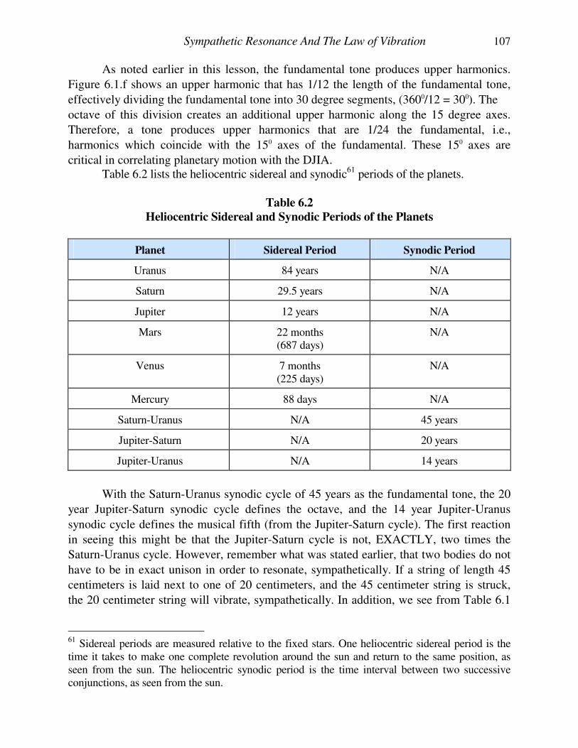
Sympathetic Resonance And The Law of Vibration 107
As noted earlier in this lesson, the fundamental tone produces upper harmonics.
Figure 6.1.f shows an upper harmonic that has 1/12 the length of the fundamental tone,
effectively dividing the fundamental tone into 30 degree segments, (3600/12 = 300). The
octave of this division creates an additional upper harmonic along the 15 degree axes.
Therefore, a tone produces upper harmonics that are 1/24 the fundamental, i.e.,
harmonics which coincide with the 150 axes of the fundamental. These 150 axes are
critical in correlating planetary motion with the DJIA. Table 6.2 lists the heliocentric sidereal and synodic61 periods of the planets.
Table 6.2
Heliocentric Sidereal and Synodic Periods of the Planets
Planet Sidereal Period Synodic Period
Uranus 84 years N/A
Saturn 29.5 years N/A
Jupiter 12 years N/A
Mars 22 months (687 days)
N/A
Venus 7 months (225 days)
N/A
Mercury 88 days N/A
Saturn-Uranus N/A 45 years
Jupiter-Saturn N/A 20 years
Jupiter-Uranus N/A 14 years
With the Saturn-Uranus synodic cycle of 45 years as the fundamental tone, the 20
year Jupiter-Saturn synodic cycle defines the octave, and the 14 year Jupiter-Uranus
synodic cycle defines the musical fifth (from the Jupiter-Saturn cycle). The first reaction
in seeing this might be that the Jupiter-Saturn cycle is not, EXACTLY, two times the
Saturn-Uranus cycle. However, remember what was stated earlier, that two bodies do not
have to be in exact unison in order to resonate, sympathetically. If a string of length 45
centimeters is laid next to one of 20 centimeters, and the 45 centimeter string is struck,
the 20 centimeter string will vibrate, sympathetically. In addition, we see from Table 6.1
61 Sidereal periods are measured relative to the fixed stars. One heliocentric sidereal period is the time it takes to make one complete revolution around the sun and return to the same position, as seen from the sun. The heliocentric synodic period is the time interval between two successive conjunctions, as seen from the sun.
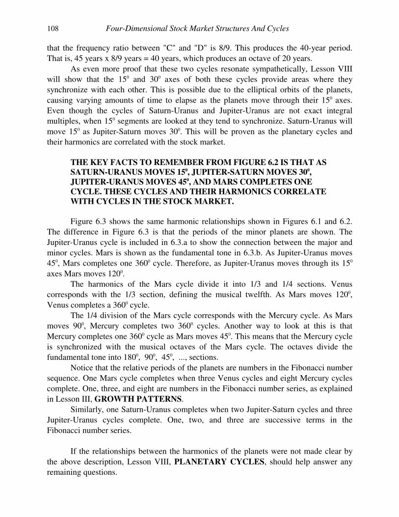
108 Four-Dimensional Stock Market Structures And Cycles
that the frequency ratio between "C" and "D" is 8/9. This produces the 40-year period.
That is, 45 years x 8/9 years = 40 years, which produces an octave of 20 years.
As even more proof that these two cycles resonate sympathetically, Lesson VIII
will show that the 150 and 300 axes of both these cycles provide areas where they
synchronize with each other. This is possible due to the elliptical orbits of the planets,
causing varying amounts of time to elapse as the planets move through their 150 axes.
Even though the cycles of Saturn-Uranus and Jupiter-Uranus are not exact integral
multiples, when 150 segments are looked at they tend to synchronize. Saturn-Uranus will
move 150 as Jupiter-Saturn moves 300. This will be proven as the planetary cycles and
their harmonics are correlated with the stock market.
THE KEY FACTS TO REMEMBER FROM FIGURE 6.2 IS THAT AS
SATURN-URANUS MOVES 150, JUPITER-SATURN MOVES 300,
JUPITER-URANUS MOVES 450, AND MARS COMPLETES ONE
CYCLE. THESE CYCLES AND THEIR HARMONICS CORRELATE
WITH CYCLES IN THE STOCK MARKET.
Figure 6.3 shows the same harmonic relationships shown in Figures 6.1 and 6.2.
The difference in Figure 6.3 is that the periods of the minor planets are shown. The
Jupiter-Uranus cycle is included in 6.3.a to show the connection between the major and
minor cycles. Mars is shown as the fundamental tone in 6.3.b. As Jupiter-Uranus moves
450, Mars completes one 3600 cycle. Therefore, as Jupiter-Uranus moves through its 150
axes Mars moves 1200.
The harmonics of the Mars cycle divide it into 1/3 and 1/4 sections. Venus
corresponds with the 1/3 section, defining the musical twelfth. As Mars moves 1200,
Venus completes a 3600 cycle.
The 1/4 division of the Mars cycle corresponds with the Mercury cycle. As Mars
moves 900, Mercury completes two 3600 cycles. Another way to look at this is that
Mercury completes one 3600 cycle as Mars moves 450. This means that the Mercury cycle
is synchronized with the musical octaves of the Mars cycle. The octaves divide the
fundamental tone into 1800, 900, 450, ..., sections.
Notice that the relative periods of the planets are numbers in the Fibonacci number
sequence. One Mars cycle completes when three Venus cycles and eight Mercury cycles
complete. One, three, and eight are numbers in the Fibonacci number series, as explained
in Lesson III, GROWTH PATTERNS.
Similarly, one Saturn-Uranus completes when two Jupiter-Saturn cycles and three
Jupiter-Uranus cycles complete. One, two, and three are successive terms in the
Fibonacci number series.
If the relationships between the harmonics of the planets were not made clear by
the above description, Lesson VIII, PLANETARY CYCLES, should help answer any
remaining questions.
Sympathetic Resonance And The Law of Vibration 109
Musical Interval / Frequency
Corresponding Ratio to
Frequency Ratio Fundamental
Figure 6.1 Musical intervals and corresponding frequency ratios.
110 Four-Dimensional Stock Market Structures And Cycles
Musical Interval / Planetary Frequency
Corresponding Cycle Ratio to
Frequency Ratio Fundamental
Figure 6.2
Musical intervals and corresponding major planetary cycles with Saturn-Uranus cycle (a) as the fundamental tone.
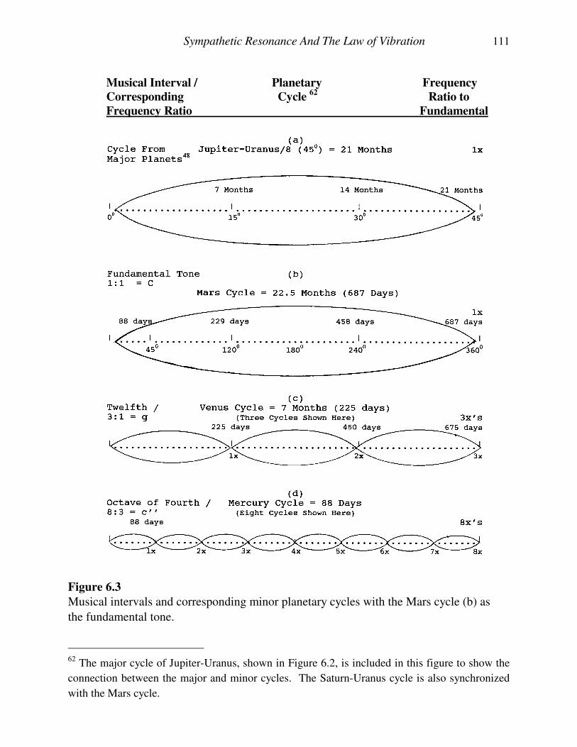
Sympathetic Resonance And The Law of Vibration 111
Musical Interval / Planetary Frequency
Corresponding Cycle 62
Ratio to
Frequency Ratio Fundamental
Figure 6.3
Musical intervals and corresponding minor planetary cycles with the Mars cycle (b) as
the fundamental tone.
62 The major cycle of Jupiter-Uranus, shown in Figure 6.2, is included in this figure to show the
connection between the major and minor cycles. The Saturn-Uranus cycle is also synchronized
with the Mars cycle.
LESSON VII CYCLES
Going far means returning. Lao Tzu (600 B.C.) ... Tao Te Ching
Is there any thing whereof it may be said, See, this is new? it hath been already of old time, which was before us.
... Ecclesiastes 1:10
INTRODUCTION The subject of financial market cycles is little understood by most market analysts. The traditional methods of Fourier transforms and percent deviations from moving averages originated with scientists and engineers. While these techniques are effective in isolating individual cyclic components of such things as radio signals or compound sound waves, they are little help when the complex topic of repetitive human behavior is studied. The cyclic component of mass human psychology becomes evident as men repeat the same mistakes committed by their parents and grandparents. When measured in mass, man not only seems incapable of learning from the mistakes of history, but also inclined to repeat the errors committed as recently as the previous generation. Financial markets are the laboratory where this mass psychology manifests in the form of price-time changes. As masses of people pool their emotions into their hopes and expectations for the future, certain geometric constructs evolve when these emotional changes are recorded as a function of time. The recurrence of behavior at similar locations on these geometric structures defines periodic law. Financial market cycles begin at a certain point in price-time and progress through their natural growth sequence until they reach completion. After which, the price-time action is contained by a new cycle. The key points to know are; when and where a cycle begins, when and where it ends, and what to expect from the new cycle. This sounds simple, but in practice there are many pitfalls that can trip up the unsuspecting analyst. This lesson will explain many cycle characteristics, of which contemporary cycle analysts are unaware. BACKGROUND REVIEW Traditional methods used by analysts to isolate the cyclic components of a financial market can be summarized in three simplified steps:63 (1) Establish a moving average from the price-time data. (2) Divide the price-time data into the moving average to obtain the percent
deviation from the moving average, obtained in step (1).
63 Reference: Cycles, Dewey.
Cycles 113
(3) Either visually or by Fourier Transform, obtain the cycles (actually rhythms) from the data in step (2).
DJIA EXAMPLE OF APPLYING CONTEMPORARY CYCLE ANALYSIS Chart VII.A shows the DJIA from 10/1/1992 to 8/27/1993. This chart has the trend channel drawn in by upper and lower parallel lines, which contain the extremes of the price swings during this time. The median between these two channel lines defines the moving average described above, in step (1), and from which the percent deviation is calculated. This moving average advances at the rate of 400 points in 200 days. That is, it defines a 2x1 diagonal angle. This type of moving average is the simplest to recognize because it is linear over the time frame being studied. As described above, in step (2), the price-time data is divided into the 2x1 moving average to obtain the percent deviation from the trend. The result of this division is shown on Chart VII.B. The third step is to determine the rhythms from the detrended data. On Chart VII.B, the first rhythm that immediately stands out is the six-week rhythm, which equals thirty trading days and is shown by vertical lines. Similarly, other rhythms can be found in this chart. The method followed above is the basic technique applied by contemporary cycle analysts. However, as will be shown in the following section, there are several problems with this approach, which can be overcome with an application of the tools presented in this course.
PROBLEMS WITH CONTEMPORARY CYCLE ANALYSIS The cycle analysis performed in the previous section contains many examples of the limitations with the approach currently used by cycle analysts. To overcome these limitations, several facts about price-time cycles must be understood. Without an understanding of the cycle characteristics listed below, it is difficult to accurately project future cyclic effects. (1) Cycles are elliptical. Hence, as described in Lesson II, THE ELLIPTICAL
NATURE OF PRICE-TIME, the price-time action either follows the major or minor axis, the upper perimeter, or the lower perimeter. While the price-time action is contained within the ellipse, the definition of the moving average is based upon which path it follows. When the price-time action moves into a new ellipse, a new moving average defines the action within that ellipse.
These ellipses are contained within larger ellipses. The paths taken by the
action within larger ellipses defines the larger moving averages.
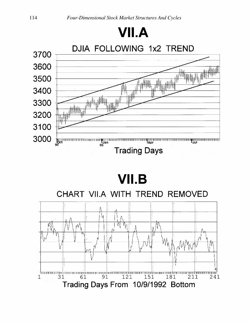
114 Four-Dimensional Stock Market Structures And Cycles
Cycles 115
(2) The origin of a cycle does not necessarily follow the terminus of the
preceding cycle because; CYCLES CAN OVERLAP AND THEY CAN
EXPERIENCE VERTICAL OFFSETS. Two overlapping cycles were shown on Chart II.A, where equilateral triangle
FIK was composed of two overlapping ellipses. The most obvious examples of vertical offsets happen after gaps. Question #3
at the end of Lesson I calculated the PTV from 1/23/1991 to 3/6/1991, shown on Chart I.D, to be an octave of the cycles occurring during this time interval. The origin of this cycle occurred on 1/23/1991, which is after the vertical offset of the gap preceding it. The origin was not at the absolute price low in 1/14/1991, even though this date was the terminus of the preceding cycle, which began on 12/21/1991.
An example of a vertical offset occurring in the opposite direction of the one
described above is shown on Chart II.A. The origin of ellipse FHIJ is at point F, which is below the price high of the preceding ellipse, CFR.
(3) The terminus of a cycle does not have to occur at its absolute price extreme.
That is, the highest price for an advancing cycle or the lowest price for a declining cycle does not necessarily represent its terminus. This was explained in Lesson II, THE ELLIPTICAL NATURE OF PRICE-TIME, and can be seen on Chart II.A at point I.
(4) Financial market cycles do not follow a constant periodicity. Due to the
elliptical nature of cycles, it takes less time to move 150 when the cycle is at its faster moving sections. Similarly, when the cycle is at the slower moving part of its cycle it takes longer for a 150 section to complete.
Another important factor causing variance in cycle periodicity is the relative
orientation of the equilateral triangles defining the axes of the mated ellipses. This topic is explained in detail later in this lesson.
PATH OF PRICE-TIME WITHIN ELLIPSE DEFINES THE MOVING AVERAGE The initial step of contemporary cycle analysis, i.e., establishing a reliable moving average, is difficult without knowledge of market geometry. As soon as a reliable moving average is established it changes, ostensibly without warning. The previous example shown on Chart VII.A used the 2x1 linear moving average. The question that cannot be reliably answered by contemporary cycle analysis is; when will this moving average change?
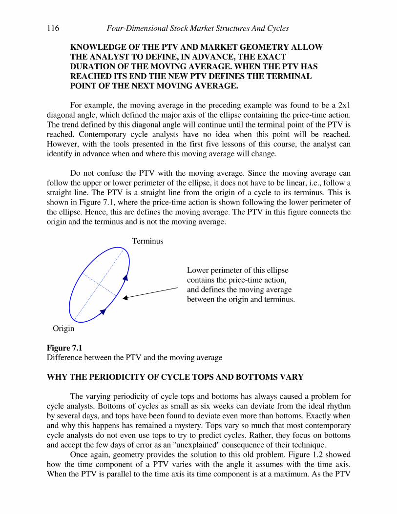
116 Four-Dimensional Stock Market Structures And Cycles
KNOWLEDGE OF THE PTV AND MARKET GEOMETRY ALLOW
THE ANALYST TO DEFINE, IN ADVANCE, THE EXACT
DURATION OF THE MOVING AVERAGE. WHEN THE PTV HAS
REACHED ITS END THE NEW PTV DEFINES THE TERMINAL
POINT OF THE NEXT MOVING AVERAGE. For example, the moving average in the preceding example was found to be a 2x1 diagonal angle, which defined the major axis of the ellipse containing the price-time action. The trend defined by this diagonal angle will continue until the terminal point of the PTV is reached. Contemporary cycle analysts have no idea when this point will be reached. However, with the tools presented in the first five lessons of this course, the analyst can identify in advance when and where this moving average will change. Do not confuse the PTV with the moving average. Since the moving average can follow the upper or lower perimeter of the ellipse, it does not have to be linear, i.e., follow a straight line. The PTV is a straight line from the origin of a cycle to its terminus. This is shown in Figure 7.1, where the price-time action is shown following the lower perimeter of the ellipse. Hence, this arc defines the moving average. The PTV in this figure connects the origin and the terminus and is not the moving average. Terminus Lower perimeter of this ellipse contains the price-time action, and defines the moving average between the origin and terminus. Origin
Figure 7.1 Difference between the PTV and the moving average
WHY THE PERIODICITY OF CYCLE TOPS AND BOTTOMS VARY The varying periodicity of cycle tops and bottoms has always caused a problem for cycle analysts. Bottoms of cycles as small as six weeks can deviate from the ideal rhythm by several days, and tops have been found to deviate even more than bottoms. Exactly when and why this happens has remained a mystery. Tops vary so much that most contemporary cycle analysts do not even use tops to try to predict cycles. Rather, they focus on bottoms and accept the few days of error as an "unexplained" consequence of their technique. Once again, geometry provides the solution to this old problem. Figure 1.2 showed how the time component of a PTV varies with the angle it assumes with the time axis. When the PTV is parallel to the time axis its time component is at a maximum. As the PTV
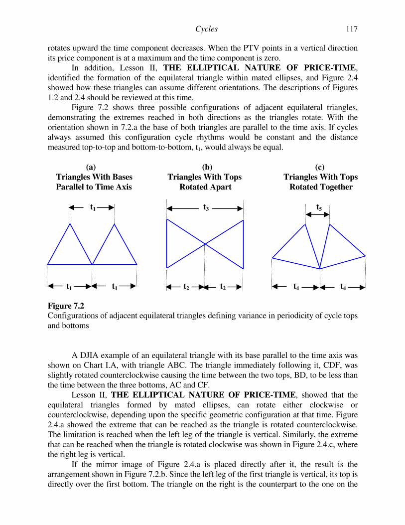
Cycles 117
rotates upward the time component decreases. When the PTV points in a vertical direction its price component is at a maximum and the time component is zero. In addition, Lesson II, THE ELLIPTICAL NATURE OF PRICE-TIME, identified the formation of the equilateral triangle within mated ellipses, and Figure 2.4 showed how these triangles can assume different orientations. The descriptions of Figures 1.2 and 2.4 should be reviewed at this time. Figure 7.2 shows three possible configurations of adjacent equilateral triangles, demonstrating the extremes reached in both directions as the triangles rotate. With the orientation shown in 7.2.a the base of both triangles are parallel to the time axis. If cycles always assumed this configuration cycle rhythms would be constant and the distance measured top-to-top and bottom-to-bottom, t1, would always be equal.
(a) (b) (c)
Triangles With Bases Triangles With Tops Triangles With Tops
Parallel to Time Axis Rotated Apart Rotated Together
t1 t3 t5
t1 t1 t2 t2 t4 t4
Figure 7.2 Configurations of adjacent equilateral triangles defining variance in periodicity of cycle tops and bottoms A DJIA example of an equilateral triangle with its base parallel to the time axis was shown on Chart I.A, with triangle ABC. The triangle immediately following it, CDF, was slightly rotated counterclockwise causing the time between the two tops, BD, to be less than the time between the three bottoms, AC and CF. Lesson II, THE ELLIPTICAL NATURE OF PRICE-TIME, showed that the equilateral triangles formed by mated ellipses, can rotate either clockwise or counterclockwise, depending upon the specific geometric configuration at that time. Figure 2.4.a showed the extreme that can be reached as the triangle is rotated counterclockwise. The limitation is reached when the left leg of the triangle is vertical. Similarly, the extreme that can be reached when the triangle is rotated clockwise was shown in Figure 2.4.c, where the right leg is vertical. If the mirror image of Figure 2.4.a is placed directly after it, the result is the arrangement shown in Figure 7.2.b. Since the left leg of the first triangle is vertical, its top is directly over the first bottom. The triangle on the right is the counterpart to the one on the
118 Four-Dimensional Stock Market Structures And Cycles
left, with its top directly over the bottom at the far right. The result of placing two triangles, rotated in opposite directions, next to each other is the maximum possible separation between the two tops, t3. An example of this type of configuration can be seen on Chart I.A, with the tops of the two triangles, IJK and KLM, rotated apart. The opposite of Figure 7.2.b is shown in Figure 7.2.c, where the tops of the two triangles are rotated toward each other. The result is a very short time interval between these two tops, t5. An example of this type of cyclic configuration can be seen on Chart I.A, with triangles EHI and IJK. Notice the spike down between the two tops, H and J. The above examples, show how the distance between tops of two rotated triangles can vary from nearly zero, as in Figure 7.2.c, to the other extreme of encompassing the entire width of the two triangles, as in Figure 7.2.b. However, even though the distance between the tops can vary greatly, the bottoms vary only slightly. The distance between the bottoms reaches its maximum when the base of the triangles are parallel to the time axis, as in Figure 7.2.a. The distance between the bottoms is at its minimum when the triangles are rotated their maximum amount in opposite directions, as shown in Figures 7.2.b and 7.2.c.64 Chart I.A provides a good example of this concept. The base of triangle ABC is parallel to the time axis, and as shown in Table 1.2, the time between these bottoms was 243.5 trading hours. In contrast, triangle IJK was rotated the maximum amount counterclockwise, since its left side is nearly vertical. Table 1.3 shows the time between the bottoms in triangle IJK was 217.0 trading hours, or 26.5 trading hours less than between the bottoms in triangle ABC. This difference of 26.5 trading hours is equal to over four trading days, a significant amount to many traders. While the bottoms defined by triangles IJK and ABC differed by four days, the shift in the tops was much more dramatic. Since triangle IJK rotated the maximum amount counterclockwise and triangle KLM rotated clockwise, the separation of the tops was close to the maximum. The time between the two tops, JL, was 347 trading hours (54 days), or over one and one-half times longer than the time between the two bottoms, IK, which equaled 217 trading hours. This type of configuration is similar to that shown in Figure 7.2.b. Compare the distance between the tops, JL, with the distance between the tops, HJ, where the triangles take the opposite configuration. The time between the two tops, HJ, equaled 15 trading days, or eight weeks less than JL. As time progresses, different combinations of paired triangles define the limits of the price-time action along the trend.65 Each of these pairs will have different orientations. Their degree of relative rotation defines the separation between cycle tops and bottoms.
64 For those who find that equations help make concepts clearer, the following relationships exist in Figure 7.2.
t1 > t2 ; t2 = t4 ; t3 = t2 + t2
65 Paired triangles are not the same as "mated ellipses". Two mated ellipses form an equilateral triangle. Two equilateral triangles form a pair.
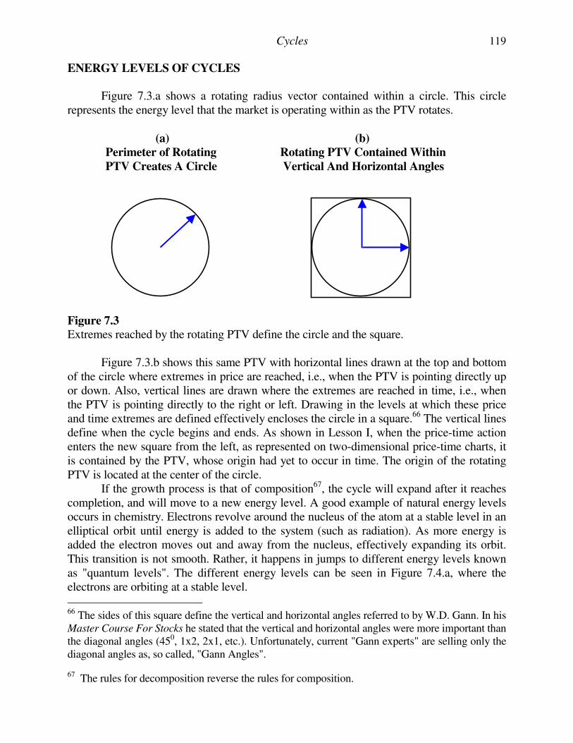
Cycles 119
ENERGY LEVELS OF CYCLES Figure 7.3.a shows a rotating radius vector contained within a circle. This circle represents the energy level that the market is operating within as the PTV rotates.
(a) (b)
Perimeter of Rotating Rotating PTV Contained Within
PTV Creates A Circle Vertical And Horizontal Angles
Figure 7.3 Extremes reached by the rotating PTV define the circle and the square. Figure 7.3.b shows this same PTV with horizontal lines drawn at the top and bottom of the circle where extremes in price are reached, i.e., when the PTV is pointing directly up or down. Also, vertical lines are drawn where the extremes are reached in time, i.e., when the PTV is pointing directly to the right or left. Drawing in the levels at which these price and time extremes are defined effectively encloses the circle in a square.66 The vertical lines define when the cycle begins and ends. As shown in Lesson I, when the price-time action enters the new square from the left, as represented on two-dimensional price-time charts, it is contained by the PTV, whose origin had yet to occur in time. The origin of the rotating PTV is located at the center of the circle. If the growth process is that of composition67, the cycle will expand after it reaches completion, and will move to a new energy level. A good example of natural energy levels occurs in chemistry. Electrons revolve around the nucleus of the atom at a stable level in an elliptical orbit until energy is added to the system (such as radiation). As more energy is added the electron moves out and away from the nucleus, effectively expanding its orbit. This transition is not smooth. Rather, it happens in jumps to different energy levels known as "quantum levels". The different energy levels can be seen in Figure 7.4.a, where the electrons are orbiting at a stable level.
66 The sides of this square define the vertical and horizontal angles referred to by W.D. Gann. In his Master Course For Stocks he stated that the vertical and horizontal angles were more important than the diagonal angles (450, 1x2, 2x1, etc.). Unfortunately, current "Gann experts" are selling only the diagonal angles as, so called, "Gann Angles".
67 The rules for decomposition reverse the rules for composition.
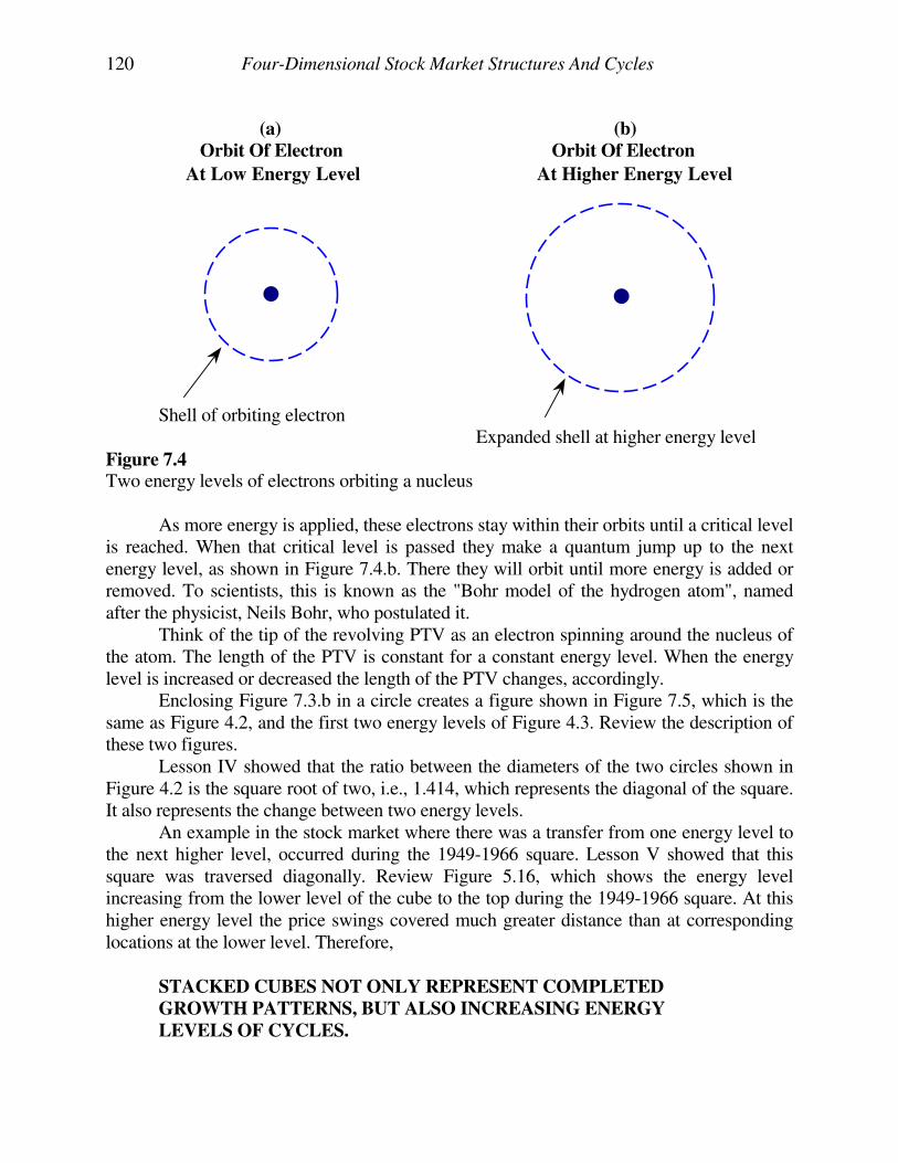
120 Four-Dimensional Stock Market Structures And Cycles
(a) (b)
Orbit Of Electron Orbit Of Electron
At Low Energy Level At Higher Energy Level Shell of orbiting electron Expanded shell at higher energy level
Figure 7.4 Two energy levels of electrons orbiting a nucleus As more energy is applied, these electrons stay within their orbits until a critical level is reached. When that critical level is passed they make a quantum jump up to the next energy level, as shown in Figure 7.4.b. There they will orbit until more energy is added or removed. To scientists, this is known as the "Bohr model of the hydrogen atom", named after the physicist, Neils Bohr, who postulated it. Think of the tip of the revolving PTV as an electron spinning around the nucleus of the atom. The length of the PTV is constant for a constant energy level. When the energy level is increased or decreased the length of the PTV changes, accordingly. Enclosing Figure 7.3.b in a circle creates a figure shown in Figure 7.5, which is the same as Figure 4.2, and the first two energy levels of Figure 4.3. Review the description of these two figures. Lesson IV showed that the ratio between the diameters of the two circles shown in Figure 4.2 is the square root of two, i.e., 1.414, which represents the diagonal of the square. It also represents the change between two energy levels. An example in the stock market where there was a transfer from one energy level to the next higher level, occurred during the 1949-1966 square. Lesson V showed that this square was traversed diagonally. Review Figure 5.16, which shows the energy level increasing from the lower level of the cube to the top during the 1949-1966 square. At this higher energy level the price swings covered much greater distance than at corresponding locations at the lower level. Therefore,
STACKED CUBES NOT ONLY REPRESENT COMPLETED
GROWTH PATTERNS, BUT ALSO INCREASING ENERGY
LEVELS OF CYCLES.
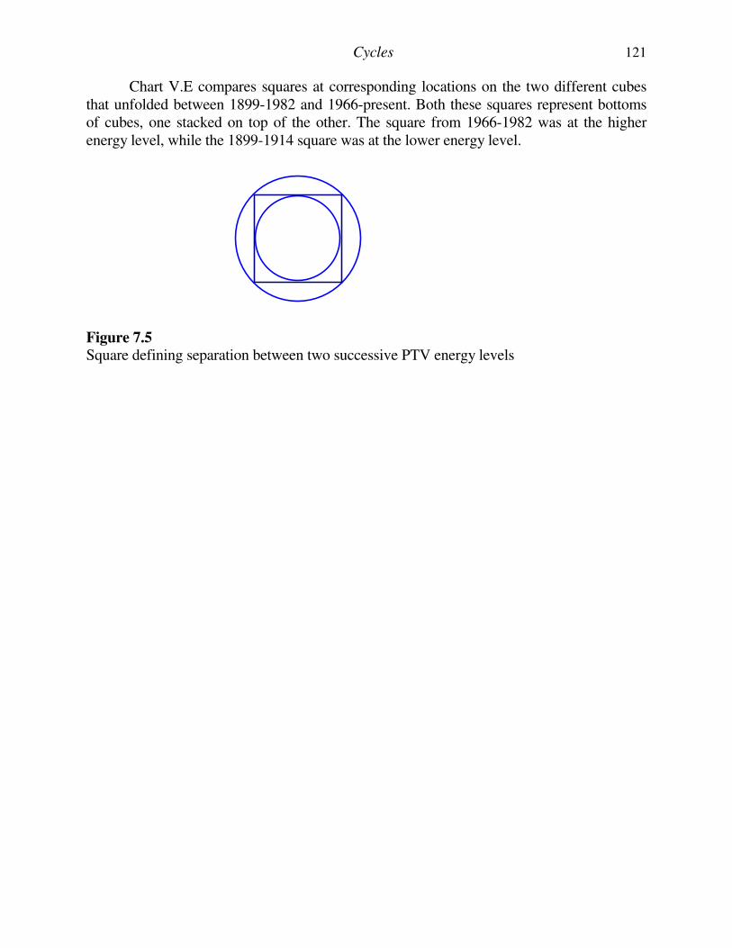
Cycles 121
Chart V.E compares squares at corresponding locations on the two different cubes that unfolded between 1899-1982 and 1966-present. Both these squares represent bottoms of cubes, one stacked on top of the other. The square from 1966-1982 was at the higher energy level, while the 1899-1914 square was at the lower energy level.
Figure 7.5 Square defining separation between two successive PTV energy levels
LESSON VIII PLANETARY CYCLES
The ears of man were intended to follow harmonious movements, just as his eyes were intended to detect the motions
of the heavenly bodies, those two being sister sciences, as the Pythagoreans declare.
Plato (347 B.C.) ...Republic
INTRODUCTION Lesson VI showed that the relative motions of the planets exist in harmonic ratios. This lesson will show that these periods and their harmonic ratios are synchronized with cycles in the stock market.68 The author spent several years researching potential correlations between geocentric motions of the planets and stock market cycles. The conclusion drawn from this research was that techniques using geocentric positions produce inconsistent results. Analysts using geocentric data claim their results are correct fifty or sixty percent of the time and consider that conclusive evidence of the efficacy of their techniques. It is the author's belief that a fifty or sixty percent correlation is nothing worthy of risking money on. In contrast, the heliocentric positions of the planets produce a clear and consistent correlation with stock market turning points. Therefore, only heliocentric data is used for all work in this lesson and throughout this course. This lesson begins with the large planetary cycles to define the larger market trends. After these larger trends are established, the cycles of the smaller planets will be progressively analyzed until the correlation between the Mercury cycle and the stock market is explained. This means that when the larger cycles are studied the smaller cycles will also be exerting their influence. This will cause some deviation at certain points, as a turning point in the stock market is delayed or advanced by one of the smaller cycles. Therefore, when studying precise dates of turning points the larger cycles must have a "window" of tolerance larger than that of the smaller cycles. This should be nothing new for students of cycle analysis. The explanation has been included here for those relatively new to the subject. As the duration of the cycles become progressively smaller, the "window" of tolerance becomes correspondingly smaller, until even data recorded by the minute can be used for accurate predictions. As mentioned in Lesson V, GEOMETRIC STRUCTURES, there is no practical limitation to the size of the time frame to which these techniques can be applied.
68 W.D. Gann used the motions of the planets as a market timing tool. The cycles listed in his Master
Course for Stocks correspond with the periods of the planets. While Gann claimed the planets were the "cause" of market activity, the author makes no such contention. Rather, it is demonstrated that a synchronicity exists between the relative motions of the planets and financial market activity.
Planetary Cycles 123
When enough expertise is obtained markets can be timed to within four minutes of resolution. This is well within the reliability of recorded data.69 To begin the analysis only monthly charts will be used. This will eliminate, as much as possible, the distortions caused by the smaller cycles. ON A MONTHLY CHART ALL VISIBLE STOCK MARKET CYCLES
ARE EXPLAINED BY THE HELIOCENTRIC SIDEREAL AND
SYNODIC MOTIONS OF THE THREE MAJOR PLANETS; URANUS,
SATURN, AND JUPITER. The periods of these cycles and their harmonics are listed in the following section. The correspondence between the harmonics of these cycles is diagramed in Figure 6.2.
BACKGROUND REVIEW Excluding the Earth and the planets orbiting beyond Uranus, there are three major planets: (1) Jupiter (2) Saturn (3) Uranus And three minor planets: (4) Mercury (5) Venus (6) Mars These are the planets that will be used to determine the cycles that are synchronous with the stock market. The motions of the major planets are synchronized with the major cycles in the stock market, and the motions of the minor planets are synchronized with the minor cycles. The periods of the planets are defined by two common systems of measurement. The synodic period measures the time period between two successive conjunctions of two planets. The sidereal period measures the time period of a planet with respect to the fixed stars. Both these systems of measurement have significance in cycle analysis. The synodic and sidereal periods of the major planets that are synchronized with stock market cycles are listed below, along with their harmonic divisions.
69 Four minutes is, approximately, how long it takes the Earth to rotate one degree. The details of how to narrow down the projected window to this small a time frame is scheduled to be included in the next volume of this home-study course. For now, accurate timing within one or two days is the objective.
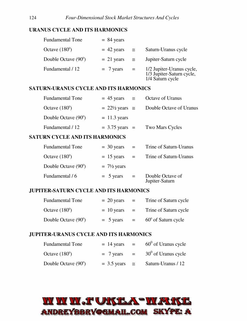
124 Four-Dimensional Stock Market Structures And Cycles
URANUS CYCLE AND ITS HARMONICS Fundamental Tone = 84 years Octave (1800) = 42 years ≅ Saturn-Uranus cycle Double Octave (900) = 21 years ≅ Jupiter-Saturn cycle Fundamental / 12 = 7 years = 1/2 Jupiter-Uranus cycle, 1/3 Jupiter-Saturn cycle, 1/4 Saturn cycle SATURN-URANUS CYCLE AND ITS HARMONICS Fundamental Tone = 45 years ≅ Octave of Uranus Octave (1800) = 22½ years ≅ Double Octave of Uranus Double Octave (900) = 11.3 years Fundamental / 12 = 3.75 years = Two Mars Cycles SATURN CYCLE AND ITS HARMONICS Fundamental Tone = 30 years = Trine of Saturn-Uranus Octave (1800) = 15 years = Trine of Saturn-Uranus Double Octave (900) = 7½ years Fundamental / 6 = 5 years = Double Octave of Jupiter-Saturn JUPITER-SATURN CYCLE AND ITS HARMONICS Fundamental Tone = 20 years = Trine of Saturn cycle Octave (1800) = 10 years = Trine of Saturn cycle Double Octave (900) = 5 years = 600 of Saturn cycle JUPITER-URANUS CYCLE AND ITS HARMONICS Fundamental Tone = 14 years = 600 of Uranus cycle Octave (1800) = 7 years = 300 of Uranus cycle Double Octave (900) = 3.5 years ≅ Saturn-Uranus / 12
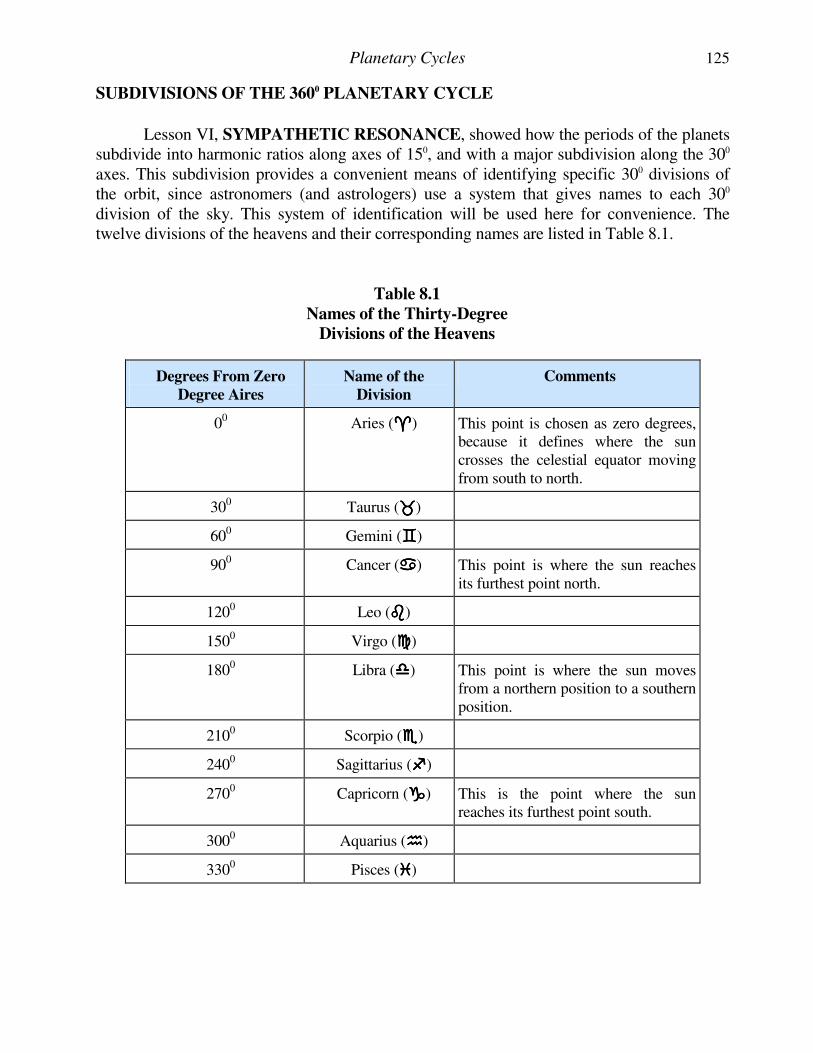
Planetary Cycles 125
SUBDIVISIONS OF THE 3600 PLANETARY CYCLE
Lesson VI, SYMPATHETIC RESONANCE, showed how the periods of the planets subdivide into harmonic ratios along axes of 150, and with a major subdivision along the 300 axes. This subdivision provides a convenient means of identifying specific 300 divisions of the orbit, since astronomers (and astrologers) use a system that gives names to each 300 division of the sky. This system of identification will be used here for convenience. The twelve divisions of the heavens and their corresponding names are listed in Table 8.1.
Table 8.1
Names of the Thirty-Degree
Divisions of the Heavens
Degrees From Zero
Degree Aires
Name of the
Division
Comments
00 Aries (����) This point is chosen as zero degrees, because it defines where the sun crosses the celestial equator moving from south to north.
300 Taurus (����)
600 Gemini (����)
900 Cancer (����) This point is where the sun reaches its furthest point north.
1200 Leo (����)
1500 Virgo (����)
1800 Libra (����) This point is where the sun moves from a northern position to a southern position.
2100 Scorpio (����)
2400 Sagittarius ()
2700 Capricorn () This is the point where the sun reaches its furthest point south.
3000 Aquarius (����)
3300 Pisces (����)
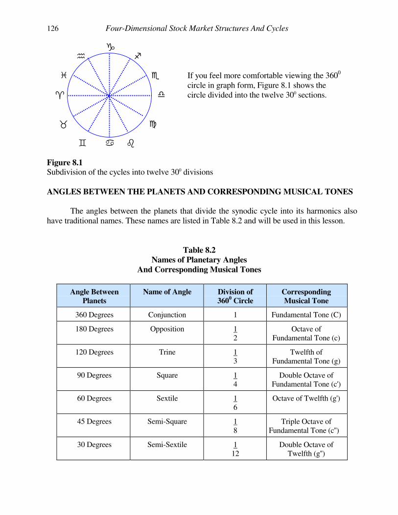
126 Four-Dimensional Stock Market Structures And Cycles
� � � If you feel more comfortable viewing the 3600
circle in graph form, Figure 8.1 shows the � � circle divided into the twelve 300 sections. � � � � �
Figure 8.1 Subdivision of the cycles into twelve 300 divisions
ANGLES BETWEEN THE PLANETS AND CORRESPONDING MUSICAL TONES The angles between the planets that divide the synodic cycle into its harmonics also have traditional names. These names are listed in Table 8.2 and will be used in this lesson.
Table 8.2
Names of Planetary Angles
And Corresponding Musical Tones
Angle Between
Planets
Name of Angle Division of
3600 Circle
Corresponding
Musical Tone
360 Degrees Conjunction 1 Fundamental Tone (C)
180 Degrees Opposition 1 2
Octave of Fundamental Tone (c)
120 Degrees Trine 1 3
Twelfth of Fundamental Tone (g)
90 Degrees Square 1 4
Double Octave of Fundamental Tone (c')
60 Degrees Sextile 1 6
Octave of Twelfth (g')
45 Degrees Semi-Square 1 8
Triple Octave of Fundamental Tone (c'')
30 Degrees Semi-Sextile 1 12
Double Octave of Twelfth (g'')
Planetary Cycles 127
PLANETARY CYCLES AND THE FOUR-DIMENSIONAL STOCK MARKET
Traditional cycle analysts have noted how cycles appear in the stock market, repeat
several times, then suddenly disappear. After a period of time these cycles reappear with a
phase shift from their original value, repeat for several rhythms, then disappear again. This
problem of disappearing cycles has confused cycle researchers, literally, for centuries.70
Astrologers used planetary cycles to predict wheat prices at least as far back as the
thirteenth century. Even these astrologers wrote about the phenomenon of disappearing
cycles.
The four-dimensional understanding of financial markets explains the phenomenon
of disappearing cycles.
CYCLES REPEAT ALONG THE FACE OF THE GEOMETRIC
STRUCTURE THAT IS PASSING THROUGH MAN'S PERCEPTION
AT THAT TIME. WHEN THE FACE OF THIS STRUCTURE IS
COMPLETE THE STRUCTURE ROTATES TO EXPOSE THE
NEXT FACE OF THE STRUCTURE. THE CYCLES ON THIS NEW
FACE HAVE A PHASE SHIFT FROM THE CYCLES ON THE
PREVIOUS FACE.
The tools developed in Part I of this course, PRICE-TIME STRUCTURES, allow
the analyst to identify his relative location within the price-time structure unfolding. More
importantly, accurate future projections can be made predicting when the face of the
structure will complete and hence, cycle phase shifts can be anticipated.
The fact that the periodicity and phase of a cycle are dependant upon the face of the
geometric structure will be proven in this lesson as cycles are identified in the stock market
that repeat along the faces of structures, identified in Lesson V, GEOMETRIC
STRUCTURES. These cycles experienced their phase shifts at the points identified in
Lesson V as a completed face of the geometric structure under construction. When the new
face rotates into view market analysts are often caught waiting for cycle tops or bottoms
that never arrive. That is because they based their projections on a set of conditions that no
longer exist. When the face of the structure is complete it rotates out of view, taking with it
the conditions that existed on that face.
70 Do not confuse disappearing cycles with the phenomenon of "beats". Beats are the result of two or more cycles interfering destructively, to reduce or eliminate their net effect. The concept of beats will be covered further in Lesson IX, COMPOSITE CYCLES. The phenomenon of disappearing cycles has nothing to do with beats. This is proven because when the cycle reappears it has a phase shift. Phase shifts do not occur with beats.
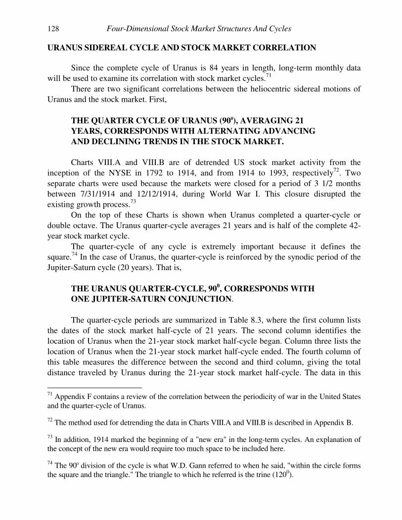
128 Four-Dimensional Stock Market Structures And Cycles
URANUS SIDEREAL CYCLE AND STOCK MARKET CORRELATION
Since the complete cycle of Uranus is 84 years in length, long-term monthly data
will be used to examine its correlation with stock market cycles.71
There are two significant correlations between the heliocentric sidereal motions of
Uranus and the stock market. First,
THE QUARTER CYCLE OF URANUS (900), AVERAGING 21
YEARS, CORRESPONDS WITH ALTERNATING ADVANCING
AND DECLINING TRENDS IN THE STOCK MARKET.
Charts VIII.A and VIII.B are of detrended US stock market activity from the
inception of the NYSE in 1792 to 1914, and from 1914 to 1993, respectively72. Two
separate charts were used because the markets were closed for a period of 3 1/2 months
between 7/31/1914 and 12/12/1914, during World War I. This closure disrupted the
existing growth process.73
On the top of these Charts is shown when Uranus completed a quarter-cycle or
double octave. The Uranus quarter-cycle averages 21 years and is half of the complete 42-
year stock market cycle.
The quarter-cycle of any cycle is extremely important because it defines the
square.74 In the case of Uranus, the quarter-cycle is reinforced by the synodic period of the
Jupiter-Saturn cycle (20 years). That is,
THE URANUS QUARTER-CYCLE, 900, CORRESPONDS WITH
ONE JUPITER-SATURN CONJUNCTION.
The quarter-cycle periods are summarized in Table 8.3, where the first column lists
the dates of the stock market half-cycle of 21 years. The second column identifies the
location of Uranus when the 21-year stock market half-cycle began. Column three lists the
location of Uranus when the 21-year stock market half-cycle ended. The fourth column of
this table measures the difference between the second and third column, giving the total
distance traveled by Uranus during the 21-year stock market half-cycle. The data in this
71 Appendix F contains a review of the correlation between the periodicity of war in the United States and the quarter-cycle of Uranus.
72 The method used for detrending the data in Charts VIII.A and VIII.B is described in Appendix B.
73 In addition, 1914 marked the beginning of a "new era" in the long-term cycles. An explanation of the concept of the new era would require too much space to be included here.
74 The 900 division of the cycle is what W.D. Gann referred to when he said, "within the circle forms the square and the triangle." The triangle to which he referred is the trine (1200).
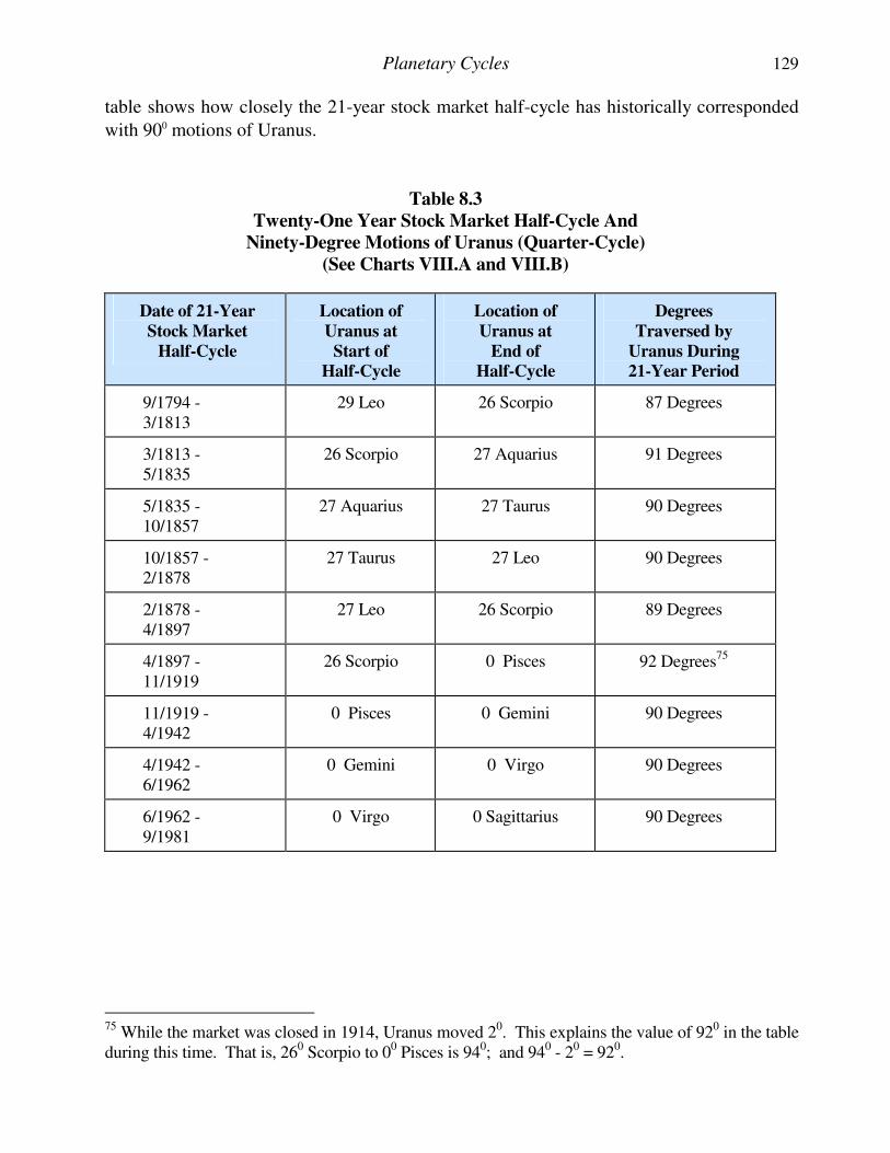
Planetary Cycles 129
table shows how closely the 21-year stock market half-cycle has historically corresponded
with 900 motions of Uranus.
Table 8.3
Twenty-One Year Stock Market Half-Cycle And
Ninety-Degree Motions of Uranus (Quarter-Cycle)
(See Charts VIII.A and VIII.B)
Date of 21-Year
Stock Market
Half-Cycle
Location of
Uranus at
Start of
Half-Cycle
Location of
Uranus at
End of
Half-Cycle
Degrees
Traversed by
Uranus During
21-Year Period
9/1794 - 3/1813
29 Leo 26 Scorpio 87 Degrees
3/1813 - 5/1835
26 Scorpio 27 Aquarius 91 Degrees
5/1835 - 10/1857
27 Aquarius 27 Taurus 90 Degrees
10/1857 - 2/1878
27 Taurus 27 Leo 90 Degrees
2/1878 - 4/1897
27 Leo 26 Scorpio 89 Degrees
4/1897 - 11/1919
26 Scorpio 0 Pisces 92 Degrees75
11/1919 - 4/1942
0 Pisces 0 Gemini 90 Degrees
4/1942 - 6/1962
0 Gemini 0 Virgo 90 Degrees
6/1962 - 9/1981
0 Virgo 0 Sagittarius 90 Degrees
75 While the market was closed in 1914, Uranus moved 20. This explains the value of 920 in the table during this time. That is, 260 Scorpio to 00 Pisces is 940; and 940 - 20 = 920.
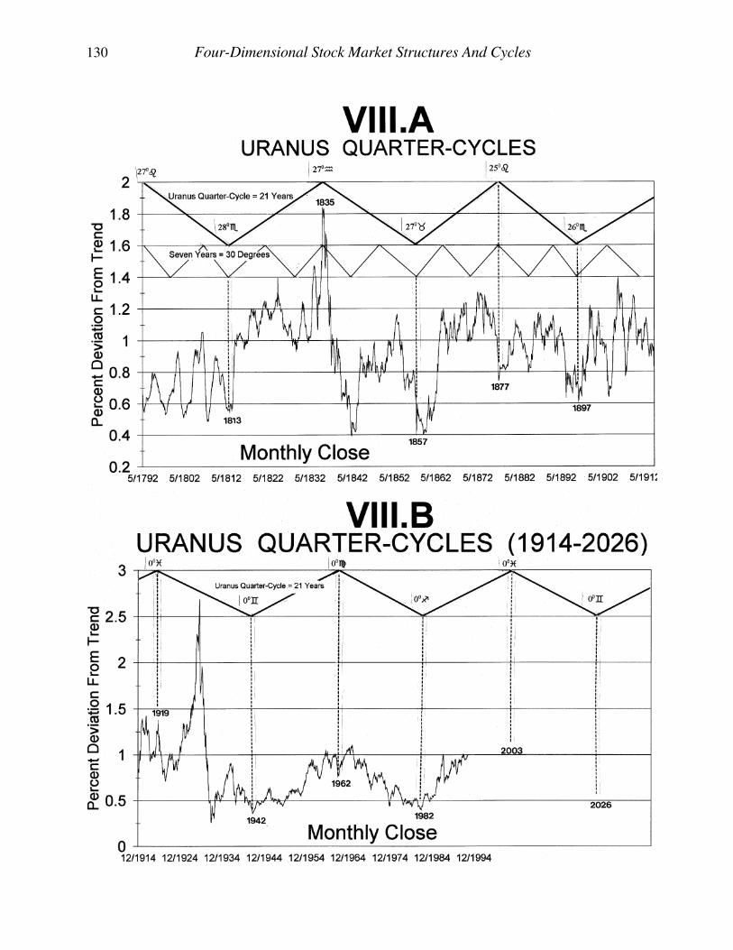
130 Four-Dimensional Stock Market Structures And Cycles
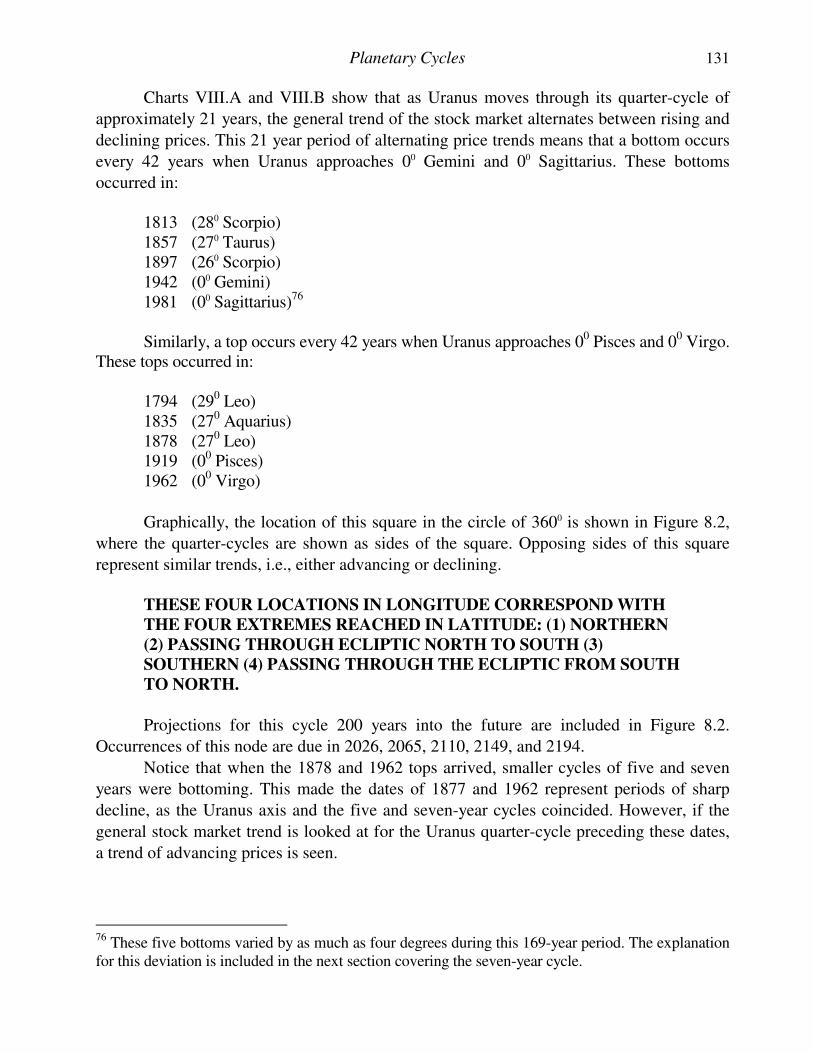
Planetary Cycles 131
Charts VIII.A and VIII.B show that as Uranus moves through its quarter-cycle of
approximately 21 years, the general trend of the stock market alternates between rising and
declining prices. This 21 year period of alternating price trends means that a bottom occurs
every 42 years when Uranus approaches 00 Gemini and 00 Sagittarius. These bottoms
occurred in: 1813 (280 Scorpio) 1857 (270 Taurus) 1897 (260 Scorpio) 1942 (00 Gemini) 1981 (00 Sagittarius)76 Similarly, a top occurs every 42 years when Uranus approaches 00 Pisces and 00 Virgo. These tops occurred in: 1794 (290 Leo) 1835 (270 Aquarius) 1878 (270 Leo) 1919 (00 Pisces) 1962 (00 Virgo)
Graphically, the location of this square in the circle of 3600 is shown in Figure 8.2,
where the quarter-cycles are shown as sides of the square. Opposing sides of this square
represent similar trends, i.e., either advancing or declining. THESE FOUR LOCATIONS IN LONGITUDE CORRESPOND WITH
THE FOUR EXTREMES REACHED IN LATITUDE: (1) NORTHERN
(2) PASSING THROUGH ECLIPTIC NORTH TO SOUTH (3)
SOUTHERN (4) PASSING THROUGH THE ECLIPTIC FROM SOUTH
TO NORTH.
Projections for this cycle 200 years into the future are included in Figure 8.2.
Occurrences of this node are due in 2026, 2065, 2110, 2149, and 2194.
Notice that when the 1878 and 1962 tops arrived, smaller cycles of five and seven
years were bottoming. This made the dates of 1877 and 1962 represent periods of sharp
decline, as the Uranus axis and the five and seven-year cycles coincided. However, if the
general stock market trend is looked at for the Uranus quarter-cycle preceding these dates,
a trend of advancing prices is seen.
76 These five bottoms varied by as much as four degrees during this 169-year period. The explanation for this deviation is included in the next section covering the seven-year cycle.
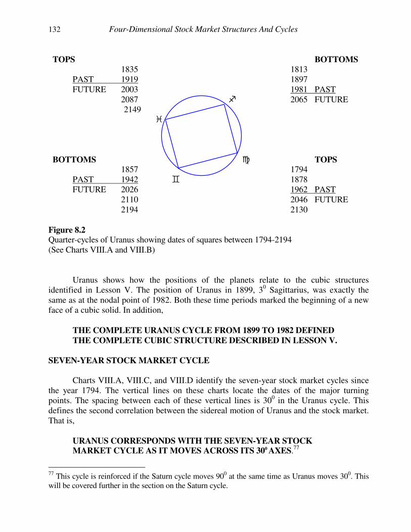
132 Four-Dimensional Stock Market Structures And Cycles
TOPS BOTTOMS
1835 1813
PAST 1919 1897 FUTURE 2003 1981 PAST 2087 2065 FUTURE 2149 �
BOTTOMS � TOPS 1857 1794 PAST 1942 � 1878 FUTURE 2026 1962 PAST 2110 2046 FUTURE 2194 2130
Figure 8.2 Quarter-cycles of Uranus showing dates of squares between 1794-2194 (See Charts VIII.A and VIII.B) Uranus shows how the positions of the planets relate to the cubic structures identified in Lesson V. The position of Uranus in 1899, 30 Sagittarius, was exactly the same as at the nodal point of 1982. Both these time periods marked the beginning of a new face of a cubic solid. In addition, THE COMPLETE URANUS CYCLE FROM 1899 TO 1982 DEFINED
THE COMPLETE CUBIC STRUCTURE DESCRIBED IN LESSON V. SEVEN-YEAR STOCK MARKET CYCLE Charts VIII.A, VIII.C, and VIII.D identify the seven-year stock market cycles since the year 1794. The vertical lines on these charts locate the dates of the major turning points. The spacing between each of these vertical lines is 300 in the Uranus cycle. This defines the second correlation between the sidereal motion of Uranus and the stock market. That is,
URANUS CORRESPONDS WITH THE SEVEN-YEAR STOCK MARKET CYCLE AS IT MOVES ACROSS ITS 300
AXES.77
77 This cycle is reinforced if the Saturn cycle moves 900 at the same time as Uranus moves 300. This will be covered further in the section on the Saturn cycle.
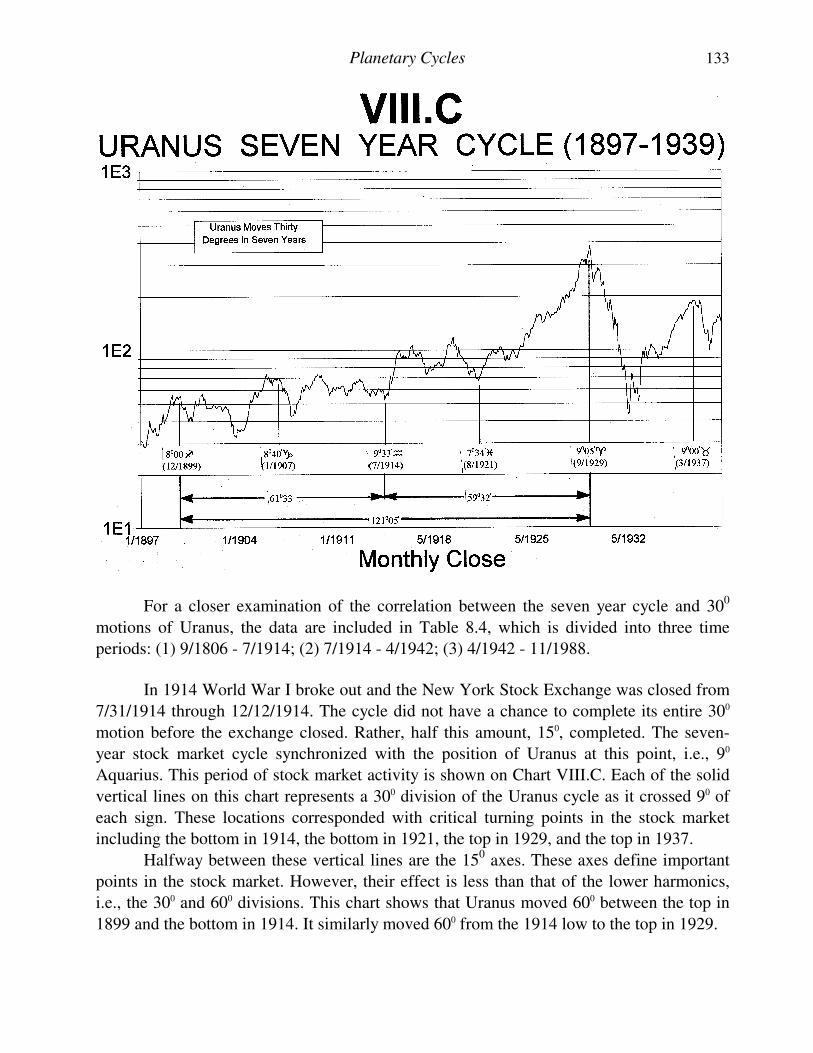
Planetary Cycles 133
For a closer examination of the correlation between the seven year cycle and 300
motions of Uranus, the data are included in Table 8.4, which is divided into three time
periods: (1) 9/1806 - 7/1914; (2) 7/1914 - 4/1942; (3) 4/1942 - 11/1988.
In 1914 World War I broke out and the New York Stock Exchange was closed from
7/31/1914 through 12/12/1914. The cycle did not have a chance to complete its entire 300
motion before the exchange closed. Rather, half this amount, 150, completed. The seven-
year stock market cycle synchronized with the position of Uranus at this point, i.e., 90
Aquarius. This period of stock market activity is shown on Chart VIII.C. Each of the solid
vertical lines on this chart represents a 300 division of the Uranus cycle as it crossed 90 of
each sign. These locations corresponded with critical turning points in the stock market
including the bottom in 1914, the bottom in 1921, the top in 1929, and the top in 1937.
Halfway between these vertical lines are the 150 axes. These axes define important
points in the stock market. However, their effect is less than that of the lower harmonics,
i.e., the 300 and 600 divisions. This chart shows that Uranus moved 600 between the top in
1899 and the bottom in 1914. It similarly moved 600 from the 1914 low to the top in 1929.
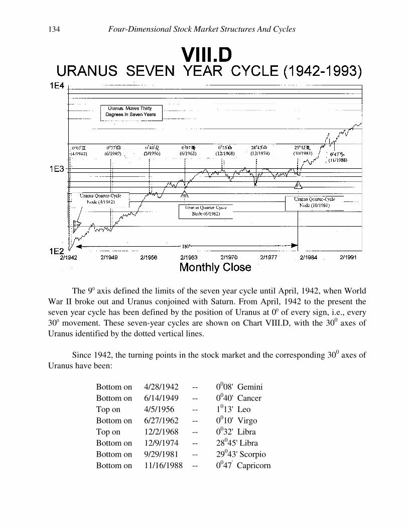
134 Four-Dimensional Stock Market Structures And Cycles
The 90 axis defined the limits of the seven year cycle until April, 1942, when World
War II broke out and Uranus conjoined with Saturn. From April, 1942 to the present the
seven year cycle has been defined by the position of Uranus at 00 of every sign, i.e., every
300 movement. These seven-year cycles are shown on Chart VIII.D, with the 300 axes of
Uranus identified by the dotted vertical lines.
Since 1942, the turning points in the stock market and the corresponding 300 axes of
Uranus have been:
Bottom on 4/28/1942 -- 0008' Gemini
Bottom on 6/14/1949 -- 0040' Cancer
Top on 4/5/1956 -- 1013' Leo
Bottom on 6/27/1962 -- 0010' Virgo
Top on 12/2/1968 -- 0032' Libra
Bottom on 12/9/1974 -- 28045' Libra
Bottom on 9/29/1981 -- 29043' Scorpio
Bottom on 11/16/1988 -- 0047' Capricorn
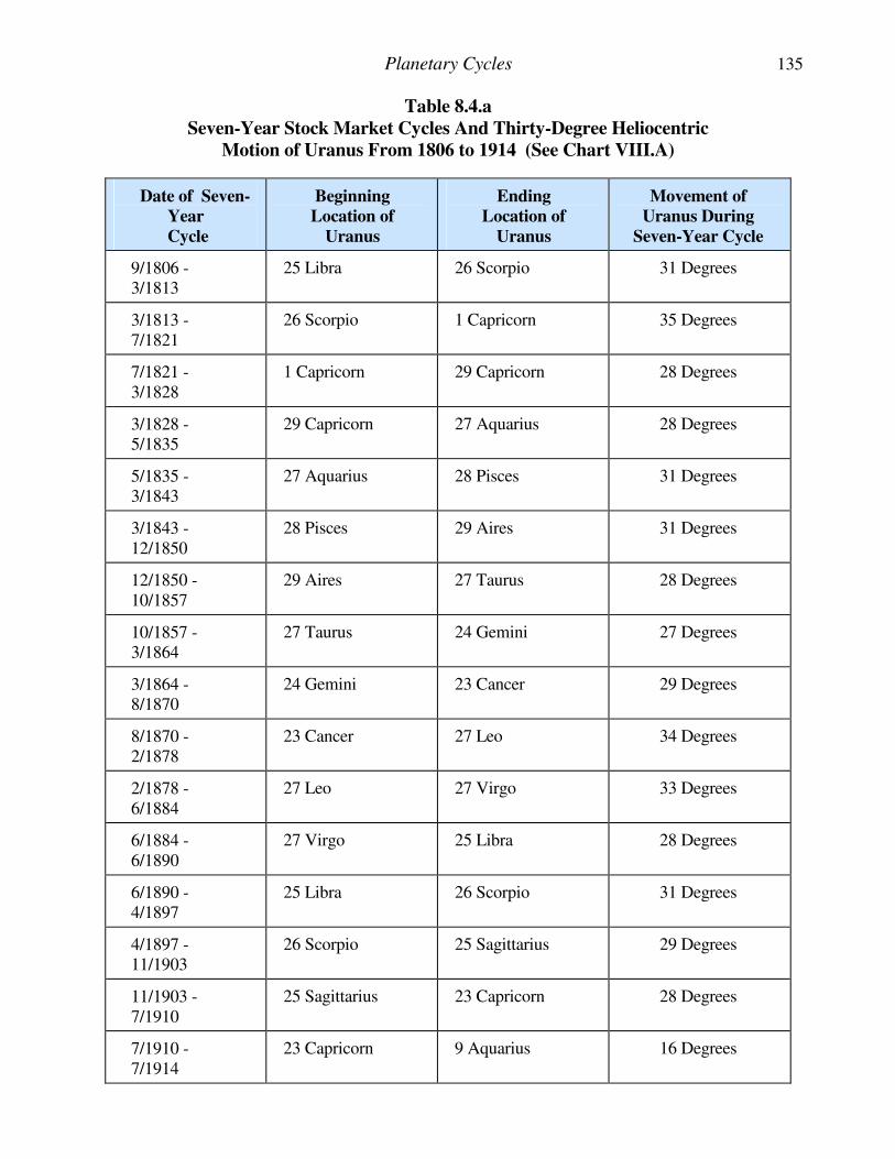
Planetary Cycles 135
Table 8.4.a
Seven-Year Stock Market Cycles And Thirty-Degree Heliocentric
Motion of Uranus From 1806 to 1914 (See Chart VIII.A)
Date of Seven-
Year
Cycle
Beginning
Location of
Uranus
Ending
Location of
Uranus
Movement of
Uranus During
Seven-Year Cycle
9/1806 - 3/1813
25 Libra 26 Scorpio 31 Degrees
3/1813 - 7/1821
26 Scorpio 1 Capricorn 35 Degrees
7/1821 - 3/1828
1 Capricorn 29 Capricorn 28 Degrees
3/1828 - 5/1835
29 Capricorn 27 Aquarius 28 Degrees
5/1835 - 3/1843
27 Aquarius 28 Pisces 31 Degrees
3/1843 - 12/1850
28 Pisces 29 Aires 31 Degrees
12/1850 - 10/1857
29 Aires 27 Taurus 28 Degrees
10/1857 - 3/1864
27 Taurus 24 Gemini 27 Degrees
3/1864 - 8/1870
24 Gemini 23 Cancer 29 Degrees
8/1870 - 2/1878
23 Cancer 27 Leo 34 Degrees
2/1878 - 6/1884
27 Leo 27 Virgo 33 Degrees
6/1884 - 6/1890
27 Virgo 25 Libra 28 Degrees
6/1890 - 4/1897
25 Libra 26 Scorpio 31 Degrees
4/1897 - 11/1903
26 Scorpio 25 Sagittarius 29 Degrees
11/1903 - 7/1910
25 Sagittarius 23 Capricorn 28 Degrees
7/1910 - 7/1914
23 Capricorn 9 Aquarius 16 Degrees
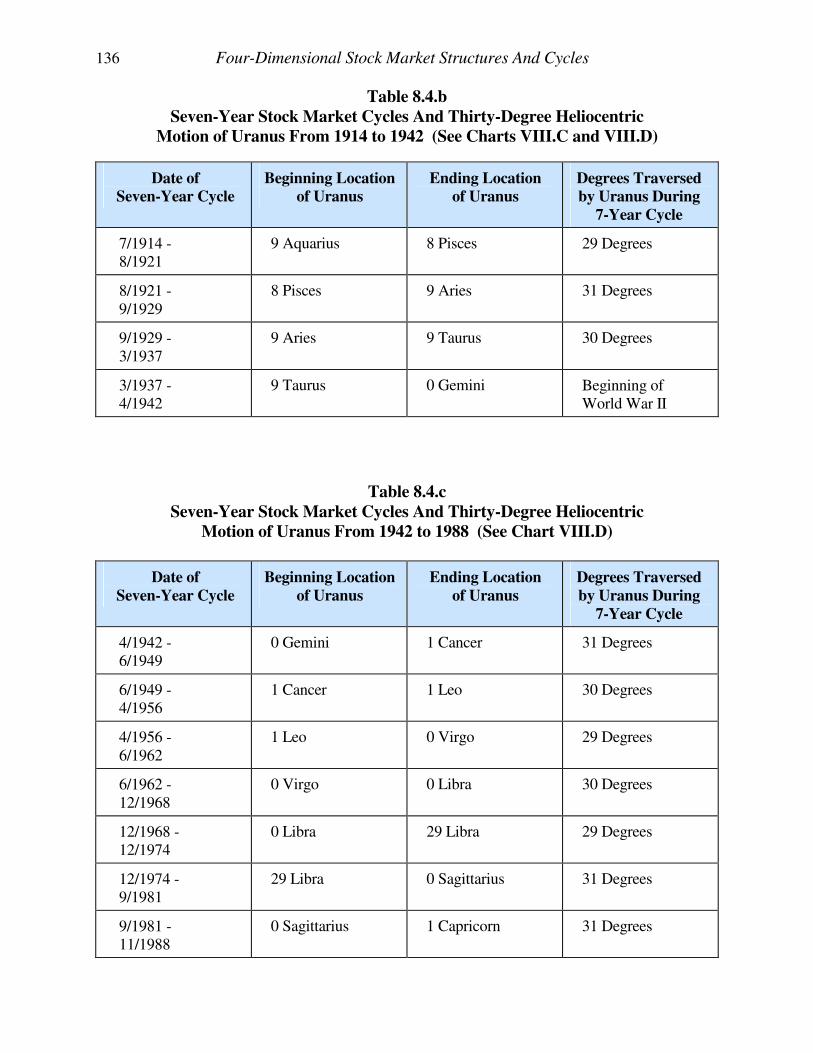
136 Four-Dimensional Stock Market Structures And Cycles
Table 8.4.b
Seven-Year Stock Market Cycles And Thirty-Degree Heliocentric
Motion of Uranus From 1914 to 1942 (See Charts VIII.C and VIII.D)
Date of
Seven-Year Cycle
Beginning Location
of Uranus
Ending Location
of Uranus
Degrees Traversed
by Uranus During
7-Year Cycle
7/1914 - 8/1921
9 Aquarius 8 Pisces 29 Degrees
8/1921 - 9/1929
8 Pisces 9 Aries 31 Degrees
9/1929 - 3/1937
9 Aries 9 Taurus 30 Degrees
3/1937 - 4/1942
9 Taurus 0 Gemini Beginning of World War II
Table 8.4.c
Seven-Year Stock Market Cycles And Thirty-Degree Heliocentric
Motion of Uranus From 1942 to 1988 (See Chart VIII.D)
Date of
Seven-Year Cycle
Beginning Location
of Uranus
Ending Location
of Uranus
Degrees Traversed
by Uranus During
7-Year Cycle
4/1942 - 6/1949
0 Gemini 1 Cancer 31 Degrees
6/1949 - 4/1956
1 Cancer 1 Leo 30 Degrees
4/1956 - 6/1962
1 Leo 0 Virgo 29 Degrees
6/1962 - 12/1968
0 Virgo 0 Libra 30 Degrees
12/1968 - 12/1974
0 Libra 29 Libra 29 Degrees
12/1974 - 9/1981
29 Libra 0 Sagittarius 31 Degrees
9/1981 - 11/1988
0 Sagittarius 1 Capricorn 31 Degrees
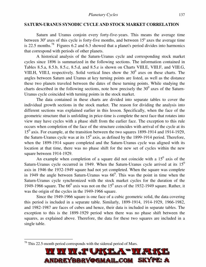
Planetary Cycles 137
SATURN-URANUS SYNODIC CYCLE AND STOCK MARKET CORRELATION
Saturn and Uranus conjoin every forty-five-years. This means the average time
between 300 axes of this cycle is forty-five months, and between 150 axes the average time
is 22.5 months.78 Figures 6.2 and 6.3 showed that a planet's period divides into harmonics
that correspond with periods of other planets.
A historical analysis of the Saturn-Uranus cycle and corresponding stock market
cycles since 1896 is summarized in the following sections. The information contained in
Tables 8.5.a, 8.5.b, 8.5.c, 8.5.d, and 8.5.e is shown on Charts VIII.E, VIII.F, and VIII.G,
VIII.H, VIII.I, respectively. Solid vertical lines show the 300 axes on these charts. The
angles between Saturn and Uranus at key turning points are listed, as well as the distance
these two planets traveled between the dates of these turning points. While studying the
charts described in the following sections, note how precisely the 300 axes of the Saturn-
Uranus cycle coincided with turning points in the stock market.
The data contained in these charts are divided into separate tables to cover the
individual growth sections in the stock market. The reason for dividing the analysis into
different sections was explained earlier in this lesson. Specifically, when the face of the
geometric structure that is unfolding in price-time is complete the next face that rotates into
view may have cycles with a phase shift from the earlier face. The exception to this rule
occurs when completion of the face of the structure coincides with arrival of the cycle at its
150 axis. For example, at the transition between the two squares 1899-1914 and 1914-1929,
the Saturn-Uranus cycle was at its 150 axis, as defined by the 1899-1914 period. Therefore,
when the 1899-1914 square completed and the Saturn-Uranus cycle was aligned with its
location at that time, there was no phase shift for the new set of cycles within the new
square between 1914-1929.
An example when completion of a square did not coincide with a 150 axis of the
Saturn-Uranus cycle occurred in 1949. When the Saturn-Uranus cycle arrived at its 150
axis in 1946 the 1932-1949 square had not yet completed. When the square was complete
in 1949 the angle between Saturn-Uranus was 660. This was the point in time when the
Saturn-Uranus cycle synchronized with the stock market cycles for the duration of the
1949-1966 square. The 660 axis was not on the 150 axes of the 1932-1949 square. Rather, it
was the origin of the cycles in the 1949-1966 square.
Since the 1949-1966 square is one face of a cubic geometric solid, the data covering
this period is included in a separate table. Similarly, 1899-1914, 1914-1929, 1966-1982,
and 1982-1987 are faces of cubes and hence, their data is included in separate tables. The
exception to this is the 1899-1929 period when there was no phase shift between the
squares, as explained above. Therefore, the data for these two squares are included in a
single table.
78 This 22.5-month period corresponds with the sidereal period of Mars.
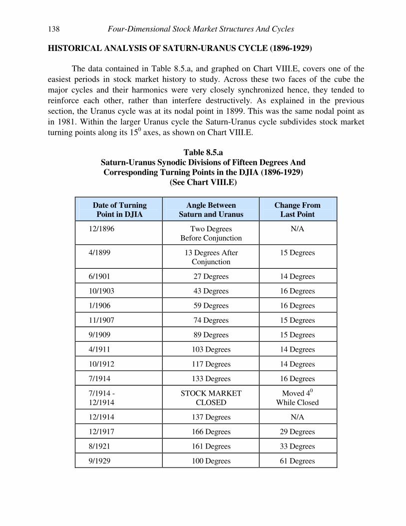
138 Four-Dimensional Stock Market Structures And Cycles
HISTORICAL ANALYSIS OF SATURN-URANUS CYCLE (1896-1929)
The data contained in Table 8.5.a, and graphed on Chart VIII.E, covers one of the
easiest periods in stock market history to study. Across these two faces of the cube the
major cycles and their harmonics were very closely synchronized hence, they tended to
reinforce each other, rather than interfere destructively. As explained in the previous
section, the Uranus cycle was at its nodal point in 1899. This was the same nodal point as
in 1981. Within the larger Uranus cycle the Saturn-Uranus cycle subdivides stock market
turning points along its 150 axes, as shown on Chart VIII.E.
Table 8.5.a
Saturn-Uranus Synodic Divisions of Fifteen Degrees And
Corresponding Turning Points in the DJIA (1896-1929)
(See Chart VIII.E)
Date of Turning
Point in DJIA
Angle Between
Saturn and Uranus
Change From
Last Point
12/1896 Two Degrees Before Conjunction
N/A
4/1899 13 Degrees After Conjunction
15 Degrees
6/1901 27 Degrees 14 Degrees
10/1903 43 Degrees 16 Degrees
1/1906 59 Degrees 16 Degrees
11/1907 74 Degrees 15 Degrees
9/1909 89 Degrees 15 Degrees
4/1911 103 Degrees 14 Degrees
10/1912 117 Degrees 14 Degrees
7/1914 133 Degrees 16 Degrees
7/1914 - 12/1914
STOCK MARKET CLOSED
Moved 40 While Closed
12/1914 137 Degrees N/A
12/1917 166 Degrees 29 Degrees
8/1921 161 Degrees 33 Degrees
9/1929 100 Degrees 61 Degrees
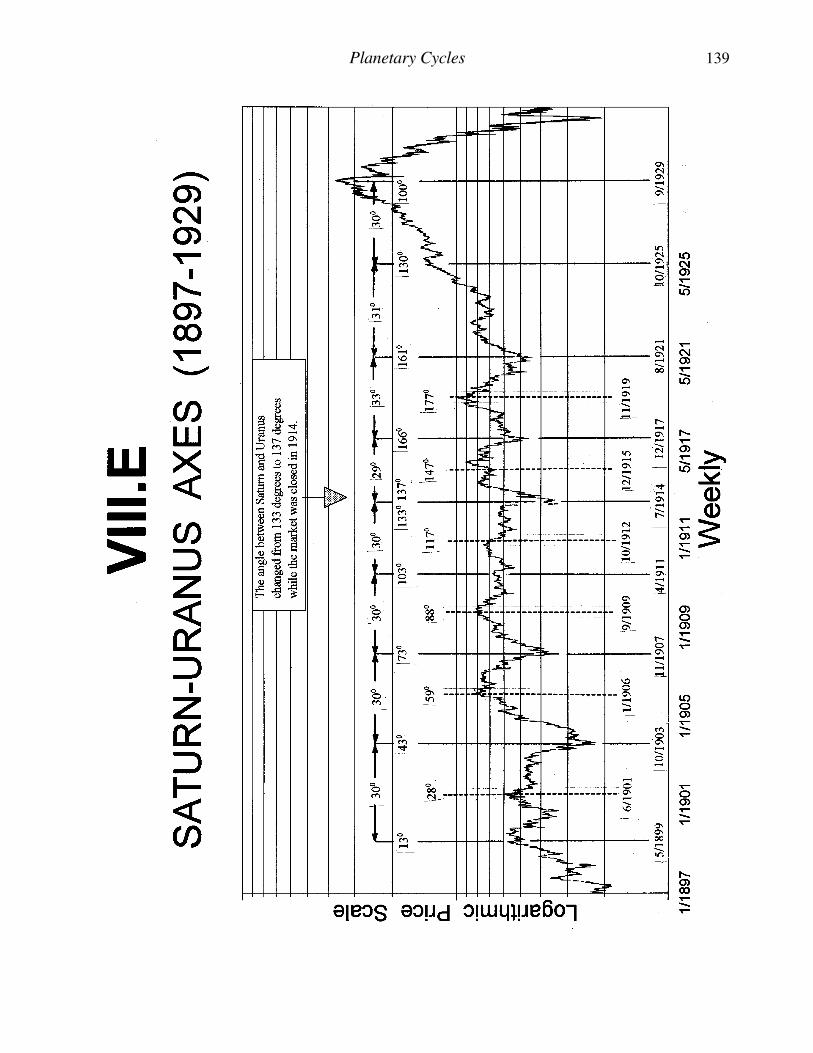
Planetary Cycles 139
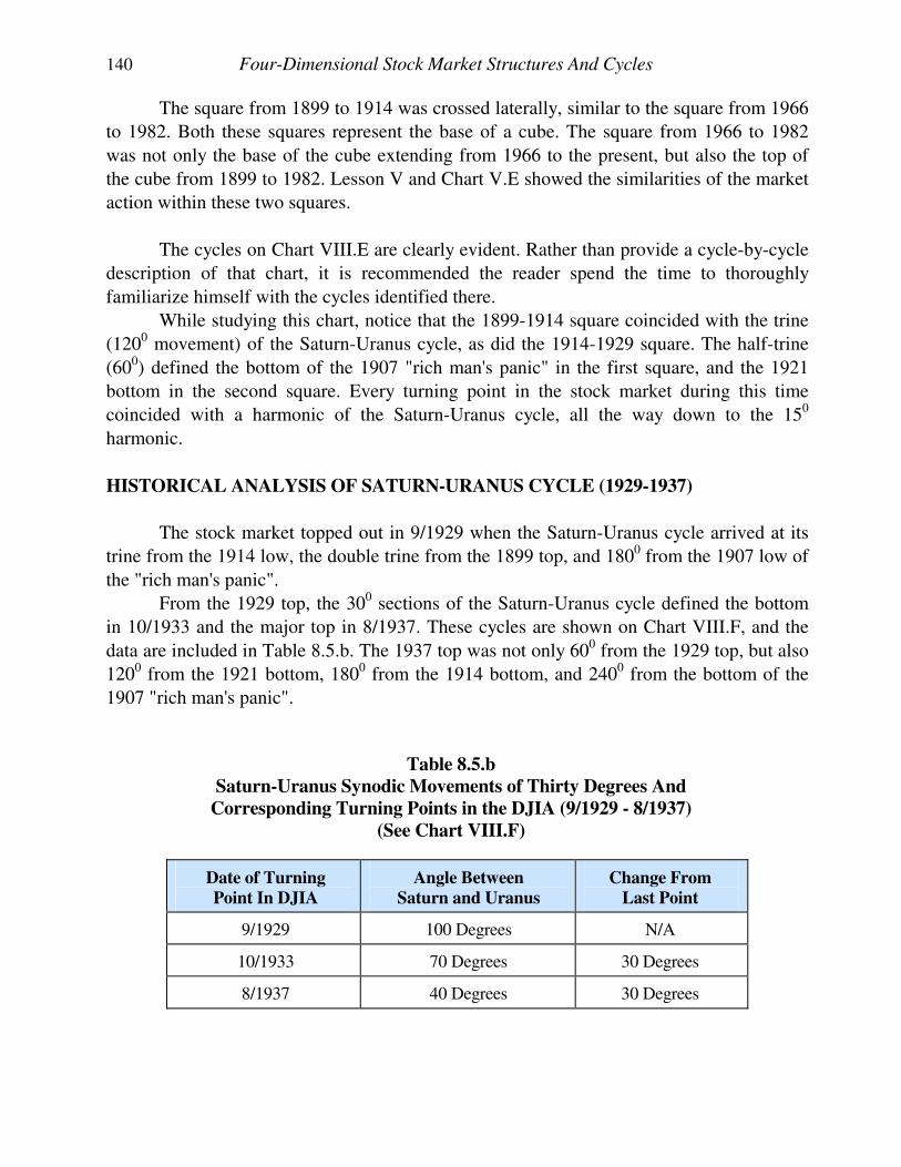
140 Four-Dimensional Stock Market Structures And Cycles
The square from 1899 to 1914 was crossed laterally, similar to the square from 1966
to 1982. Both these squares represent the base of a cube. The square from 1966 to 1982
was not only the base of the cube extending from 1966 to the present, but also the top of
the cube from 1899 to 1982. Lesson V and Chart V.E showed the similarities of the market
action within these two squares.
The cycles on Chart VIII.E are clearly evident. Rather than provide a cycle-by-cycle
description of that chart, it is recommended the reader spend the time to thoroughly
familiarize himself with the cycles identified there.
While studying this chart, notice that the 1899-1914 square coincided with the trine
(1200 movement) of the Saturn-Uranus cycle, as did the 1914-1929 square. The half-trine
(600) defined the bottom of the 1907 "rich man's panic" in the first square, and the 1921
bottom in the second square. Every turning point in the stock market during this time
coincided with a harmonic of the Saturn-Uranus cycle, all the way down to the 150
harmonic.
HISTORICAL ANALYSIS OF SATURN-URANUS CYCLE (1929-1937)
The stock market topped out in 9/1929 when the Saturn-Uranus cycle arrived at its
trine from the 1914 low, the double trine from the 1899 top, and 1800 from the 1907 low of
the "rich man's panic".
From the 1929 top, the 300 sections of the Saturn-Uranus cycle defined the bottom
in 10/1933 and the major top in 8/1937. These cycles are shown on Chart VIII.F, and the
data are included in Table 8.5.b. The 1937 top was not only 600 from the 1929 top, but also
1200 from the 1921 bottom, 1800 from the 1914 bottom, and 2400 from the bottom of the
1907 "rich man's panic".
Table 8.5.b
Saturn-Uranus Synodic Movements of Thirty Degrees And
Corresponding Turning Points in the DJIA (9/1929 - 8/1937)
(See Chart VIII.F)
Date of Turning
Point In DJIA
Angle Between
Saturn and Uranus
Change From
Last Point
9/1929 100 Degrees N/A
10/1933 70 Degrees 30 Degrees
8/1937 40 Degrees 30 Degrees
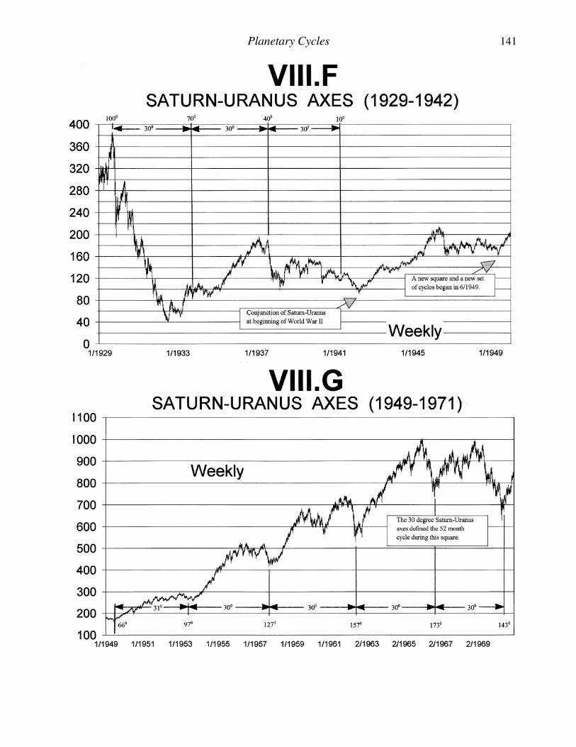
Planetary Cycles 141
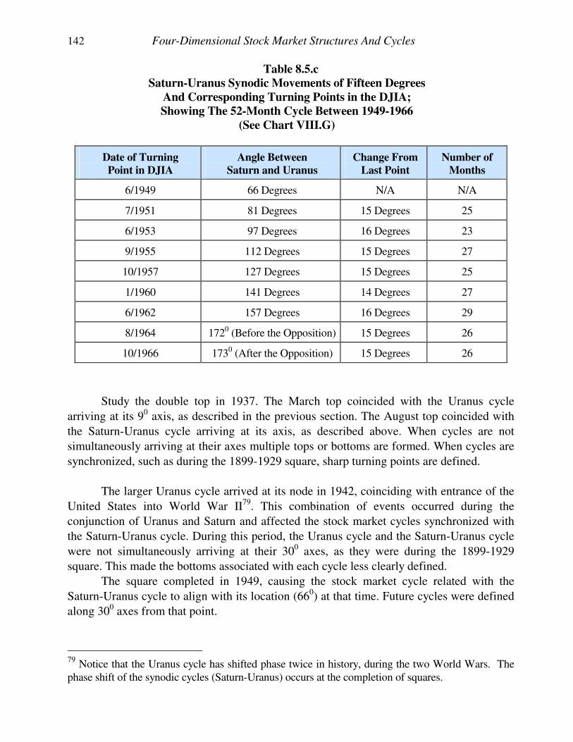
142 Four-Dimensional Stock Market Structures And Cycles
Table 8.5.c
Saturn-Uranus Synodic Movements of Fifteen Degrees
And Corresponding Turning Points in the DJIA;
Showing The 52-Month Cycle Between 1949-1966
(See Chart VIII.G)
Date of Turning
Point in DJIA
Angle Between
Saturn and Uranus
Change From
Last Point
Number of
Months
6/1949 66 Degrees N/A N/A
7/1951 81 Degrees 15 Degrees 25
6/1953 97 Degrees 16 Degrees 23
9/1955 112 Degrees 15 Degrees 27
10/1957 127 Degrees 15 Degrees 25
1/1960 141 Degrees 14 Degrees 27
6/1962 157 Degrees 16 Degrees 29
8/1964 1720 (Before the Opposition) 15 Degrees 26
10/1966 1730 (After the Opposition) 15 Degrees 26
Study the double top in 1937. The March top coincided with the Uranus cycle
arriving at its 90 axis, as described in the previous section. The August top coincided with
the Saturn-Uranus cycle arriving at its axis, as described above. When cycles are not
simultaneously arriving at their axes multiple tops or bottoms are formed. When cycles are
synchronized, such as during the 1899-1929 square, sharp turning points are defined.
The larger Uranus cycle arrived at its node in 1942, coinciding with entrance of the
United States into World War II79. This combination of events occurred during the
conjunction of Uranus and Saturn and affected the stock market cycles synchronized with
the Saturn-Uranus cycle. During this period, the Uranus cycle and the Saturn-Uranus cycle
were not simultaneously arriving at their 300 axes, as they were during the 1899-1929
square. This made the bottoms associated with each cycle less clearly defined.
The square completed in 1949, causing the stock market cycle related with the
Saturn-Uranus cycle to align with its location (660) at that time. Future cycles were defined
along 300 axes from that point.
79
Notice that the Uranus cycle has shifted phase twice in history, during the two World Wars. The phase shift of the synodic cycles (Saturn-Uranus) occurs at the completion of squares.
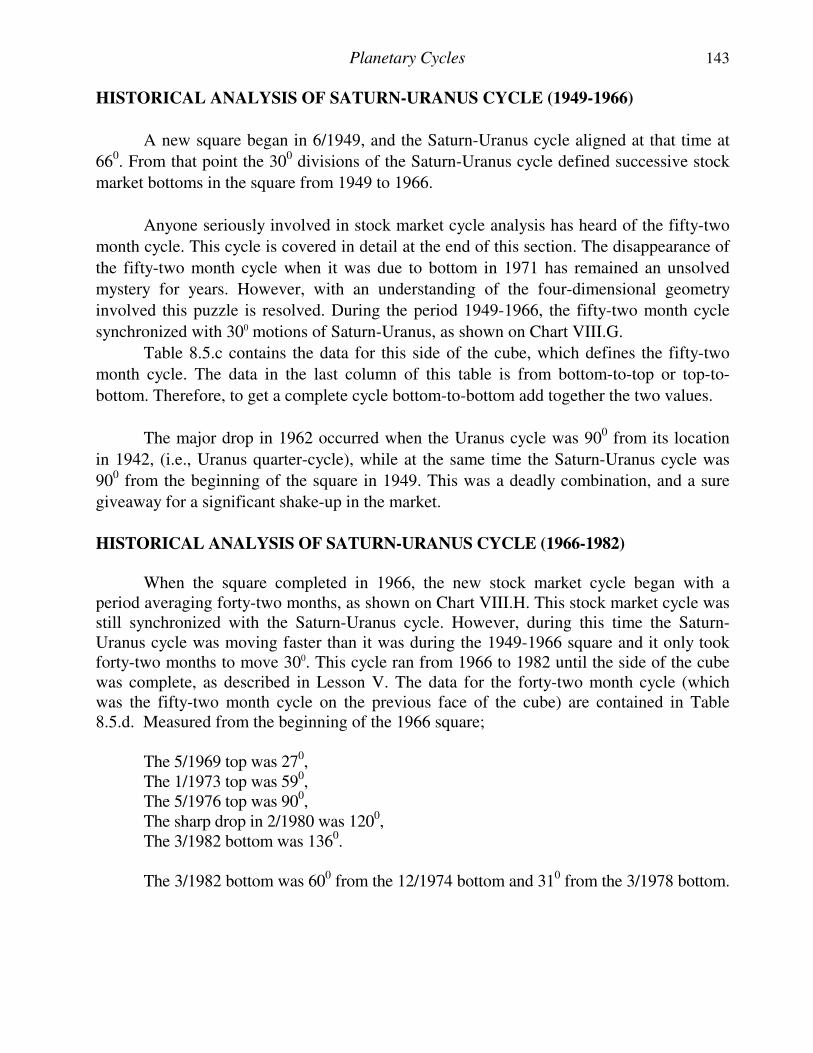
Planetary Cycles 143
HISTORICAL ANALYSIS OF SATURN-URANUS CYCLE (1949-1966)
A new square began in 6/1949, and the Saturn-Uranus cycle aligned at that time at
660. From that point the 300 divisions of the Saturn-Uranus cycle defined successive stock
market bottoms in the square from 1949 to 1966.
Anyone seriously involved in stock market cycle analysis has heard of the fifty-two
month cycle. This cycle is covered in detail at the end of this section. The disappearance of
the fifty-two month cycle when it was due to bottom in 1971 has remained an unsolved
mystery for years. However, with an understanding of the four-dimensional geometry
involved this puzzle is resolved. During the period 1949-1966, the fifty-two month cycle
synchronized with 300 motions of Saturn-Uranus, as shown on Chart VIII.G.
Table 8.5.c contains the data for this side of the cube, which defines the fifty-two
month cycle. The data in the last column of this table is from bottom-to-top or top-to-
bottom. Therefore, to get a complete cycle bottom-to-bottom add together the two values.
The major drop in 1962 occurred when the Uranus cycle was 900 from its location
in 1942, (i.e., Uranus quarter-cycle), while at the same time the Saturn-Uranus cycle was
900 from the beginning of the square in 1949. This was a deadly combination, and a sure
giveaway for a significant shake-up in the market.
HISTORICAL ANALYSIS OF SATURN-URANUS CYCLE (1966-1982) When the square completed in 1966, the new stock market cycle began with a period averaging forty-two months, as shown on Chart VIII.H. This stock market cycle was still synchronized with the Saturn-Uranus cycle. However, during this time the Saturn-Uranus cycle was moving faster than it was during the 1949-1966 square and it only took forty-two months to move 300. This cycle ran from 1966 to 1982 until the side of the cube was complete, as described in Lesson V. The data for the forty-two month cycle (which was the fifty-two month cycle on the previous face of the cube) are contained in Table 8.5.d. Measured from the beginning of the 1966 square; The 5/1969 top was 270, The 1/1973 top was 590, The 5/1976 top was 900, The sharp drop in 2/1980 was 1200, The 3/1982 bottom was 1360. The 3/1982 bottom was 600 from the 12/1974 bottom and 310 from the 3/1978 bottom.
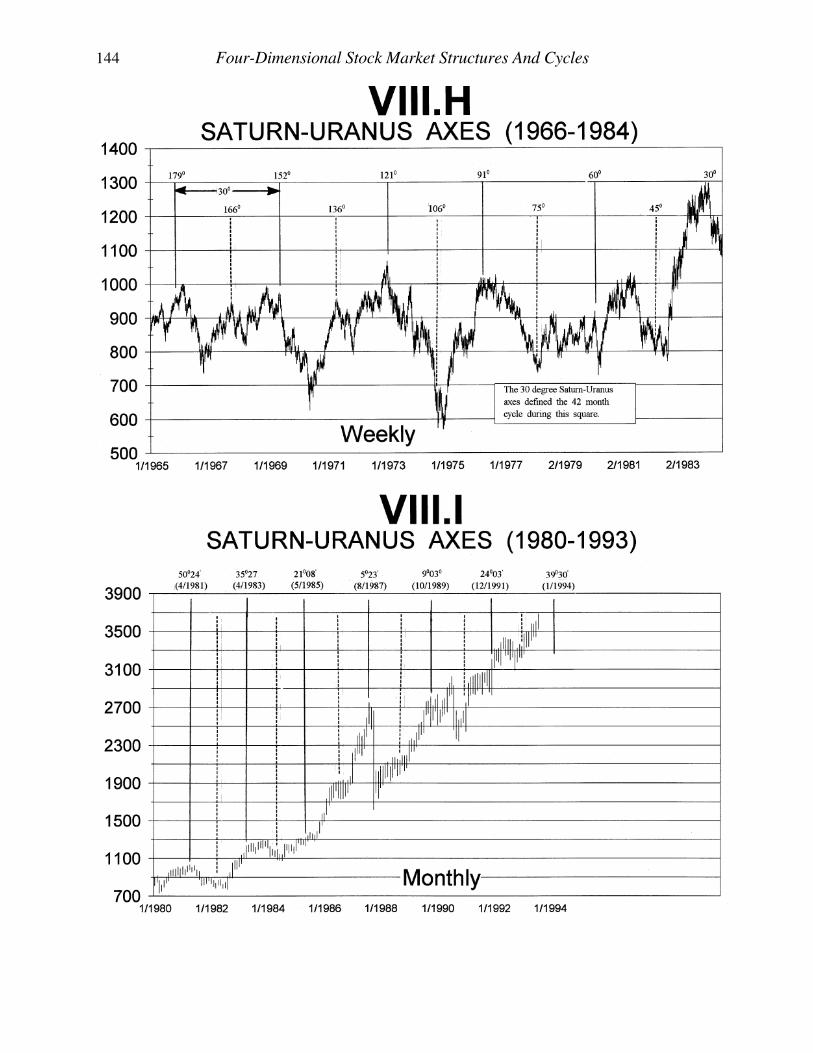
144 Four-Dimensional Stock Market Structures And Cycles
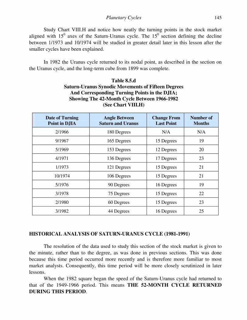
Planetary Cycles 145
Study Chart VIII.H and notice how neatly the turning points in the stock market
aligned with 150 axes of the Saturn-Uranus cycle. The 150 section defining the decline
between 1/1973 and 10/1974 will be studied in greater detail later in this lesson after the
smaller cycles have been explained.
In 1982 the Uranus cycle returned to its nodal point, as described in the section on
the Uranus cycle, and the long-term cube from 1899 was complete.
Table 8.5.d
Saturn-Uranus Synodic Movements of Fifteen Degrees
And Corresponding Turning Points in the DJIA;
Showing The 42-Month Cycle Between 1966-1982
(See Chart VIII.H)
Date of Turning
Point in DJIA
Angle Between
Saturn and Uranus
Change From
Last Point
Number of
Months
2/1966 180 Degrees N/A N/A
9/1967 165 Degrees 15 Degrees 19
5/1969 153 Degrees 12 Degrees 20
4/1971 136 Degrees 17 Degrees 23
1/1973 121 Degrees 15 Degrees 21
10/1974 106 Degrees 15 Degrees 21
5/1976 90 Degrees 16 Degrees 19
3/1978 75 Degrees 15 Degrees 22
2/1980 60 Degrees 15 Degrees 23
3/1982 44 Degrees 16 Degrees 25
HISTORICAL ANALYSIS OF SATURN-URANUS CYCLE (1981-1991)
The resolution of the data used to study this section of the stock market is given to
the minute, rather than to the degree, as was done in previous sections. This was done
because this time period occurred more recently and is therefore more familiar to most
market analysts. Consequently, this time period will be more closely scrutinized in later
lessons.
When the 1982 square began the speed of the Saturn-Uranus cycle had returned to
that of the 1949-1966 period. This means THE 52-MONTH CYCLE RETURNED
DURING THIS PERIOD.
146 Four-Dimensional Stock Market Structures And Cycles
Chart VIII.I shows the Saturn-Uranus cycle from 1981 to 1993. When the top
arrived in 4/26/1981 the Saturn-Uranus cycle was at 50024'. Thirty degrees of the Saturn-
Uranus cycle measured from this axis defined the 52-month cycle. One and one-half times
this amount (450) defined the 78-month cycle.
For example, the top in 8/25/1987 occurred at 5023', which was 45001' from the top
on 4/26/1981.
Exactly 52-months after the top on 8/25/1987 the stock market bottomed on
12/11/1991. During this time, the Saturn-Uranus cycle moved from 5023' through the
conjunction to 24003', or a distance of 29026'. The halfway point in this cycle was
10/10/1989, when the "mini-crash of 1989" occurred. This date was exactly 150 from the
12/11/1991 low. That is, 24003' - 9003' = 150.
When is the next 150 axis due? Add 450 to the 8/25/1987 top and the sum is 39037'.
This angle arrives in January, 1994. Similarly, add 150 to the 12/11/1991 bottom and you
get 39003'. Again, due in January, 1994. Or, add 900 to the 4/26/1981 high to get 39036'.
Again, due in January, 1994. The net result of this will be a turning point in January that
will be identifiable on a monthly chart.
Table 8.5.e
Saturn-Uranus Synodic Movements of Fifteen Degrees
And Corresponding Turning Points in the DJIA
Between 1981-1991 Showing The 52-Month Cycle
(See Chart VIII.I)
Date of Turning
Point in DJIA
Angle Between
Saturn and Uranus
Change From
Last Point
Number of
Months
4/26/1981 50024' N/A N/A
4/26/1983 35027' 14057' 24
5/02/1985 21008' 14019' 25
8/25/1987 5023' 15045' 27
10/10/1989 9003' 14026' 26
12/11/1991 24003' 15000' 26
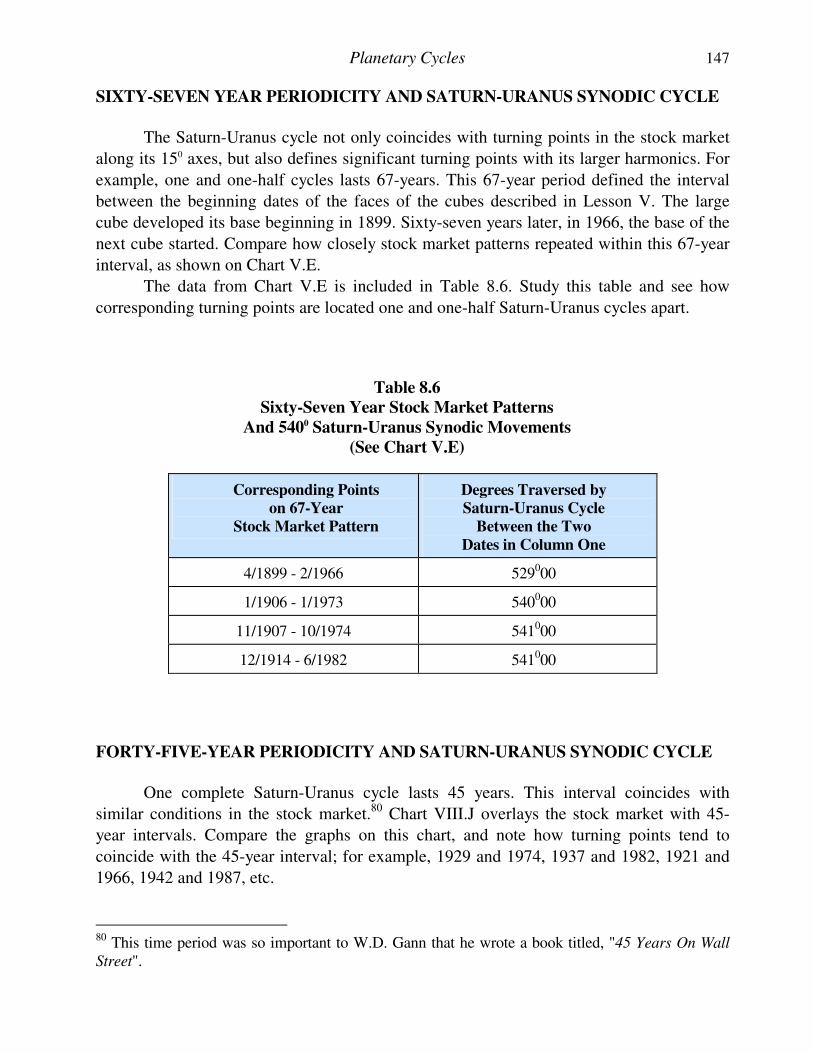
Planetary Cycles 147
SIXTY-SEVEN YEAR PERIODICITY AND SATURN-URANUS SYNODIC CYCLE
The Saturn-Uranus cycle not only coincides with turning points in the stock market
along its 150 axes, but also defines significant turning points with its larger harmonics. For
example, one and one-half cycles lasts 67-years. This 67-year period defined the interval
between the beginning dates of the faces of the cubes described in Lesson V. The large
cube developed its base beginning in 1899. Sixty-seven years later, in 1966, the base of the
next cube started. Compare how closely stock market patterns repeated within this 67-year
interval, as shown on Chart V.E.
The data from Chart V.E is included in Table 8.6. Study this table and see how
corresponding turning points are located one and one-half Saturn-Uranus cycles apart.
Table 8.6
Sixty-Seven Year Stock Market Patterns
And 5400 Saturn-Uranus Synodic Movements
(See Chart V.E)
Corresponding Points
on 67-Year
Stock Market Pattern
Degrees Traversed by
Saturn-Uranus Cycle
Between the Two
Dates in Column One
4/1899 - 2/1966 529000
1/1906 - 1/1973 540000
11/1907 - 10/1974 541000
12/1914 - 6/1982 541000
FORTY-FIVE-YEAR PERIODICITY AND SATURN-URANUS SYNODIC CYCLE
One complete Saturn-Uranus cycle lasts 45 years. This interval coincides with
similar conditions in the stock market.80 Chart VIII.J overlays the stock market with 45-
year intervals. Compare the graphs on this chart, and note how turning points tend to
coincide with the 45-year interval; for example, 1929 and 1974, 1937 and 1982, 1921 and
1966, 1942 and 1987, etc.
80 This time period was so important to W.D. Gann that he wrote a book titled, "45 Years On Wall
Street".
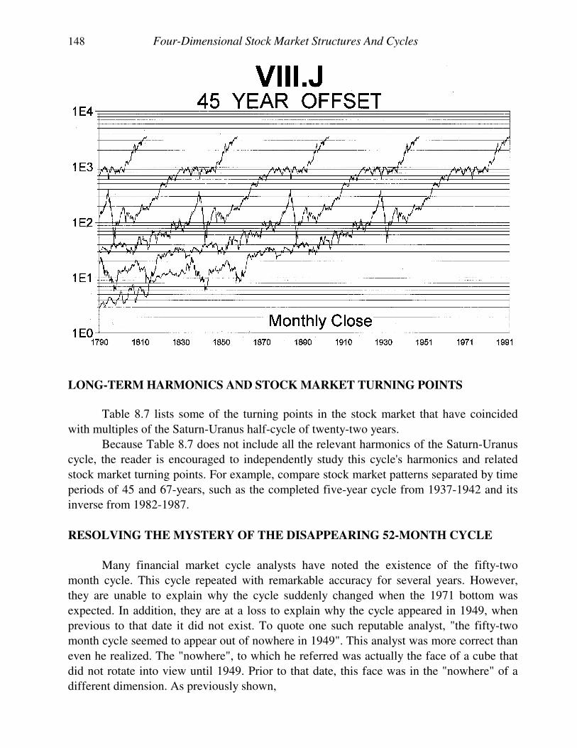
148 Four-Dimensional Stock Market Structures And Cycles
LONG-TERM HARMONICS AND STOCK MARKET TURNING POINTS
Table 8.7 lists some of the turning points in the stock market that have coincided
with multiples of the Saturn-Uranus half-cycle of twenty-two years.
Because Table 8.7 does not include all the relevant harmonics of the Saturn-Uranus
cycle, the reader is encouraged to independently study this cycle's harmonics and related
stock market turning points. For example, compare stock market patterns separated by time
periods of 45 and 67-years, such as the completed five-year cycle from 1937-1942 and its
inverse from 1982-1987.
RESOLVING THE MYSTERY OF THE DISAPPEARING 52-MONTH CYCLE
Many financial market cycle analysts have noted the existence of the fifty-two
month cycle. This cycle repeated with remarkable accuracy for several years. However,
they are unable to explain why the cycle suddenly changed when the 1971 bottom was
expected. In addition, they are at a loss to explain why the cycle appeared in 1949, when
previous to that date it did not exist. To quote one such reputable analyst, "the fifty-two
month cycle seemed to appear out of nowhere in 1949". This analyst was more correct than
even he realized. The "nowhere", to which he referred was actually the face of a cube that
did not rotate into view until 1949. Prior to that date, this face was in the "nowhere" of a
different dimension. As previously shown,
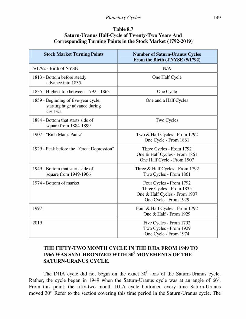
Planetary Cycles 149
Table 8.7
Saturn-Uranus Half-Cycle of Twenty-Two Years And
Corresponding Turning Points in the Stock Market (1792-2019)
Stock Market Turning Points Number of Saturn-Uranus Cycles
From the Birth of NYSE (5/1792)
5/1792 - Birth of NYSE N/A
1813 - Bottom before steady advance into 1835
One Half Cycle
1835 - Highest top between 1792 - 1863 One Cycle
1859 - Beginning of five-year cycle, starting huge advance during civil war
One and a Half Cycles
1884 - Bottom that starts side of square from 1884-1899
Two Cycles
1907 - "Rich Man's Panic" Two & Half Cycles - From 1792 One Cycle - From 1861
1929 - Peak before the "Great Depression" Three Cycles - From 1792 One & Half Cycles - From 1861 One Half Cycle - From 1907
1949 - Bottom that starts side of square from 1949-1966
Three & Half Cycles - From 1792 Two Cycles - From 1861
1974 - Bottom of market Four Cycles - From 1792 Three Cycles - From 1835 One & Half Cycles - From 1907 One Cycle - From 1929
1997 Four & Half Cycles - From 1792 One & Half - From 1929
2019 Five Cycles - From 1792 Two Cycles - From 1929 One Cycle - From 1974
THE FIFTY-TWO MONTH CYCLE IN THE DJIA FROM 1949 TO
1966 WAS SYNCHRONIZED WITH 300 MOVEMENTS OF THE
SATURN-URANUS CYCLE.
The DJIA cycle did not begin on the exact 300 axis of the Saturn-Uranus cycle.
Rather, the cycle began in 1949 when the Saturn-Uranus cycle was at an angle of 660.
From this point, the fifty-two month DJIA cycle bottomed every time Saturn-Uranus
moved 300. Refer to the section covering this time period in the Saturn-Uranus cycle. The
150 Four-Dimensional Stock Market Structures And Cycles
period from 1949 to 1966 represents a face of the cubic structure described in Lesson V,
GEOMETRIC STRUCTURES. During this time the DJIA moved across the diagonal of
square DE as shown on Chart V.B, at an angle of 440. This face of the cube completed in
1966. On that date, the new face of the cube rotated into view and the 300 axes of the
Saturn-Uranus cycle synchronized with the new DJIA cycle. This new cycle had a
periodicity of 42-months, rather than 52-months of the previous cycle. This shifting in the
length of the cycle is caused by the elliptical nature of the planets orbits. After 1966, Saturn
was moving much faster, relative to Uranus, than it was before 1966. The DJIA cycle of
42-months still corresponded with 300 movements of Saturn-Uranus, it just took less time
for that distance to be covered.
This new set of cycles began in 1966 and continued across the new face of the cube
until 1982 when that square completed. This cycle topped in 1966, 1969, 1973, 1976, and
1980. Chart VIII.H showed that each of these tops corresponded with a 300 motion of
Saturn-Uranus. Notice that tops were used for this face of the cube, while bottoms were
used for the 1949-1966 structure. This is because the 1966-1982 square represents the top
of the cubic structure, while 1949-1966 was the diagonal of a square composing a side of
the cube.
When the 1966-1982 square completed the speed of the Saturn-Uranus cycle had
increased to that of the 1949-1966 square, corresponding to the return of the 52-month
cycle at that time. The precise dates of this cycle and corresponding locations of Saturn-
Uranus are listed in Table 8.5.e.
SATURN SIDEREAL CYCLE AND STOCK MARKET CORRELATION
Saturn completes one revolution relative to the fixed stars in 29.5 years. This cycle
and its harmonics are key to stock market timing because,
FIVE-YEAR STOCK MARKET GROWTH PATTERNS ARE
SYNCHRONIZED WITH 600 MOTIONS OF SATURN.
It is critical the stock market analyst is aware of this relationship. For example, the
five-year bull market from June, 1982 to October, 1987 began when Saturn entered 210
Virgo in June, 1982 and abruptly terminated in October, 1987 when Saturn crossed 210
Scorpio, which was 600 from its position at the beginning of the bull market.
Similarly, the five-year component of the "great bull market" of the 1920's began in
May, 1924 when Saturn crossed 00 Scorpio, and continued until September, 1929 when the
600 interval had been spanned by Saturn as it crossed 00 Capricorn.
Numerous examples exist proving the correlation between the five-year stock
market cycle and the 600 interval of Saturn. Table 8.8 chronicles these five-year cycles,
since 1859. As with the Uranus cycle, the data in Table 8.8 is divided into two parts. The
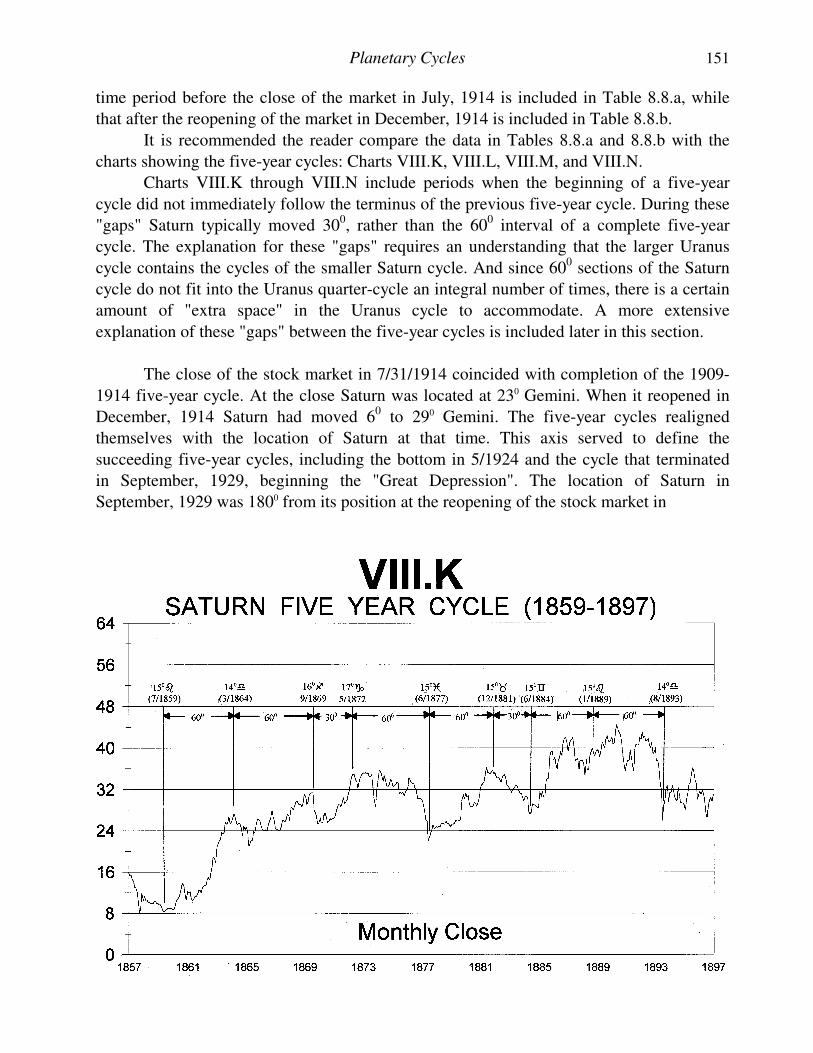
Planetary Cycles 151
time period before the close of the market in July, 1914 is included in Table 8.8.a, while
that after the reopening of the market in December, 1914 is included in Table 8.8.b.
It is recommended the reader compare the data in Tables 8.8.a and 8.8.b with the
charts showing the five-year cycles: Charts VIII.K, VIII.L, VIII.M, and VIII.N.
Charts VIII.K through VIII.N include periods when the beginning of a five-year
cycle did not immediately follow the terminus of the previous five-year cycle. During these
"gaps" Saturn typically moved 300, rather than the 600 interval of a complete five-year
cycle. The explanation for these "gaps" requires an understanding that the larger Uranus
cycle contains the cycles of the smaller Saturn cycle. And since 600 sections of the Saturn
cycle do not fit into the Uranus quarter-cycle an integral number of times, there is a certain
amount of "extra space" in the Uranus cycle to accommodate. A more extensive
explanation of these "gaps" between the five-year cycles is included later in this section.
The close of the stock market in 7/31/1914 coincided with completion of the 1909-
1914 five-year cycle. At the close Saturn was located at 230 Gemini. When it reopened in
December, 1914 Saturn had moved 60 to 290 Gemini. The five-year cycles realigned
themselves with the location of Saturn at that time. This axis served to define the
succeeding five-year cycles, including the bottom in 5/1924 and the cycle that terminated
in September, 1929, beginning the "Great Depression". The location of Saturn in
September, 1929 was 1800 from its position at the reopening of the stock market in
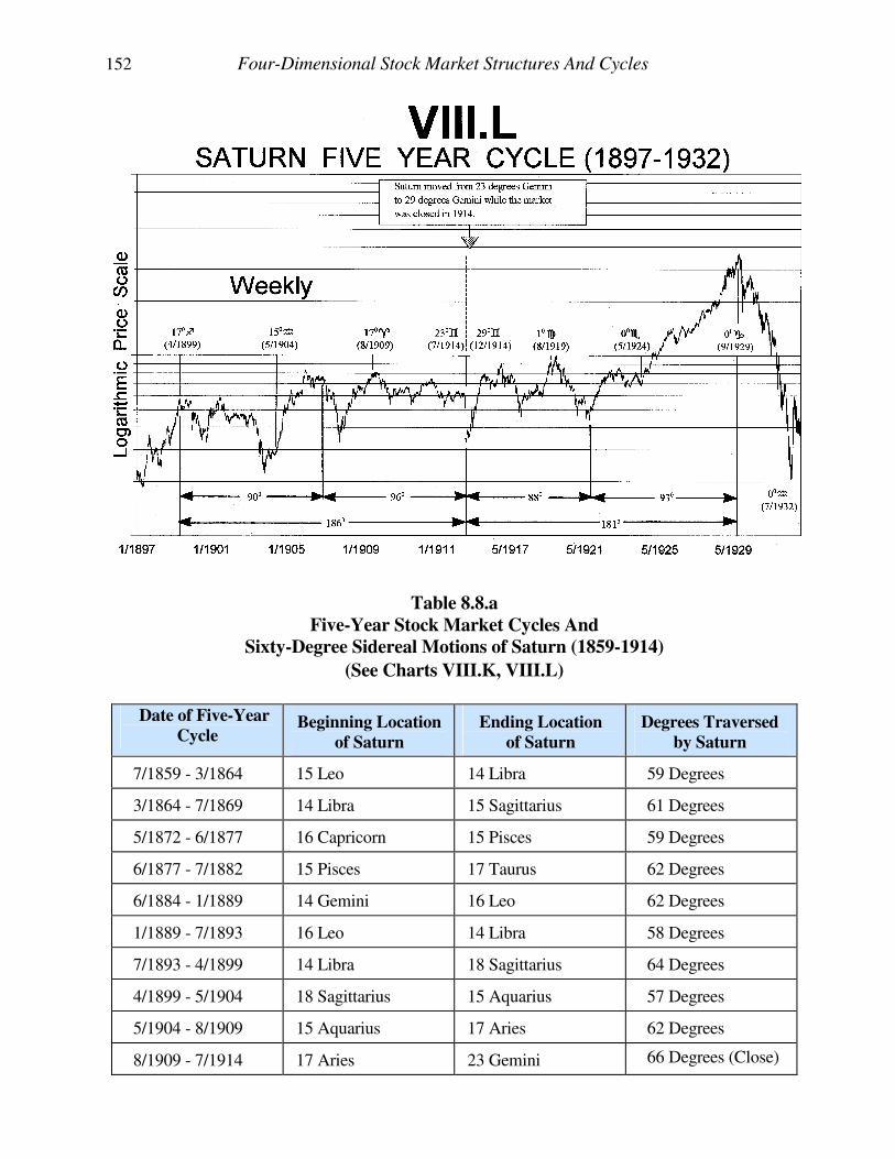
152 Four-Dimensional Stock Market Structures And Cycles
Table 8.8.a
Five-Year Stock Market Cycles And
Sixty-Degree Sidereal Motions of Saturn (1859-1914)
(See Charts VIII.K, VIII.L)
Date of Five-Year
Cycle Beginning Location
of Saturn
Ending Location
of Saturn
Degrees Traversed
by Saturn
7/1859 - 3/1864 15 Leo 14 Libra 59 Degrees
3/1864 - 7/1869 14 Libra 15 Sagittarius 61 Degrees
5/1872 - 6/1877 16 Capricorn 15 Pisces 59 Degrees
6/1877 - 7/1882 15 Pisces 17 Taurus 62 Degrees
6/1884 - 1/1889 14 Gemini 16 Leo 62 Degrees
1/1889 - 7/1893 16 Leo 14 Libra 58 Degrees
7/1893 - 4/1899 14 Libra 18 Sagittarius 64 Degrees
4/1899 - 5/1904 18 Sagittarius 15 Aquarius 57 Degrees
5/1904 - 8/1909 15 Aquarius 17 Aries 62 Degrees
8/1909 - 7/1914 17 Aries 23 Gemini 66 Degrees (Close)
Planetary Cycles 153
December, 1914 and 3600 from its position at the beginning of the square in 1899 (plus the
60 it moved while the market was closed). The 1899 top was flat during which Saturn
moved from 180 Sagittarius in 4/1899 to 260 Sagittarius 12/1899.
Cycles are easiest to study when they align with other cycles or their harmonics. In
the case of the Saturn cycle, it is easiest to identify the five-year stock market cycle when
the Uranus cycle is reaching its axes at the same time as is Saturn. One such period existed
between 1899 and 1929. This time frame is excellent to study in great detail. The Saturn
cycle for this period is shown on Chart VIII.L. And the Saturn-Uranus cycle is shown on
Chart VIII.E. Notice from these two charts, how the two cycles were aligned with each
other at major turning points in the stock market. The period from 1899 to 1914 was 1200
in the Saturn-Uranus cycle, 1800 in the Saturn cycle, and hence, 600 in the Uranus cycle.
Similarly, the period from 1914 to 1929 had identical cyclical relationships between
these two planets. During this time, Saturn moved 1800, Saturn-Uranus moved 1200, and
Uranus moved 600. Therefore, between 1899 and 1929; Saturn moved a complete cycle of
3600, Saturn-Uranus moved 2400, and Uranus moved 1200. This thirty-year period had to be
one of the easiest stock markets ever to time! Spend some time reviewing the charts
covering the cycles in this time period. This knowledge will make it easier to analyze time
frames when the cycles are not exactly aligned.
The section on the Uranus cycle showed that major bottoms in the stock
market coincide with Uranus entering Gemini and Sagittarius. These locations are 1800
apart and also coincide with major turning points in the Saturn cycle. Since the period of
Saturn is 29.5 years, its 1800 nodal areas are 15 years apart. These nodal areas have been:
Top in 9/1824 Saturn at 10 Gemini Bottom in 11/1839 Saturn at 120 Sagittarius Bottom in 12/1854 Saturn at 120 Gemini Top in 9/1869 Saturn at 170 Sagittarius Bottom in 6/1884 Saturn at 140 Gemini Top in 4/1899 Saturn at 180 Sagittarius Bottom in 7/1914 Saturn at 230 Gemini Top in 9/1929 Saturn at 29035' Sagittarius Bottom in 4/1942 Saturn at 10 Gemini Top in 8/1956 Saturn at 20 Sagittarius Top in 1/1973 Saturn at 190 Gemini
Top in 10/1987 Saturn at 210 Sagittarius
Saturn will return to this nodal area in the year 2002, which coincides with Uranus
returning to the nodal area shown in Figure 8.2.
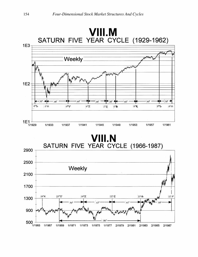
154 Four-Dimensional Stock Market Structures And Cycles
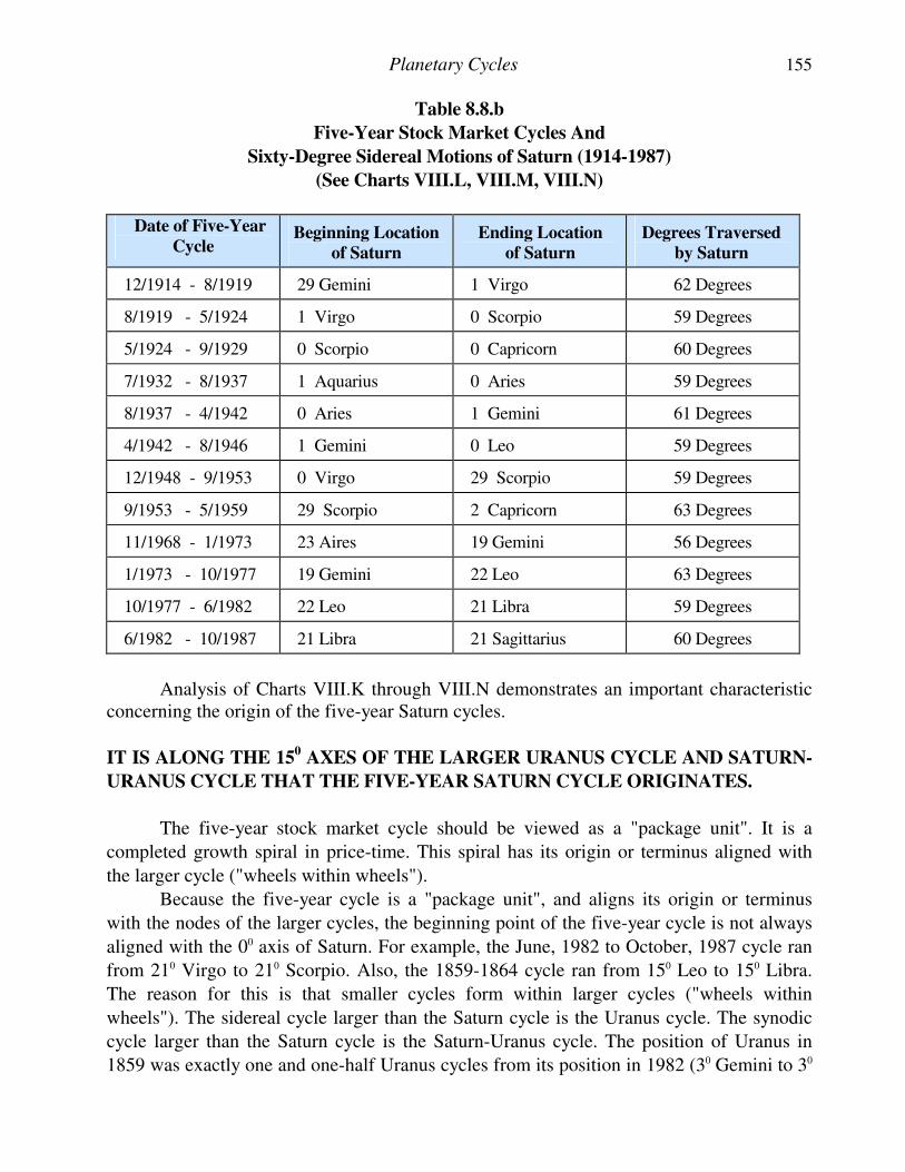
Planetary Cycles 155
Table 8.8.b
Five-Year Stock Market Cycles And
Sixty-Degree Sidereal Motions of Saturn (1914-1987)
(See Charts VIII.L, VIII.M, VIII.N)
Date of Five-Year
Cycle Beginning Location
of Saturn
Ending Location
of Saturn
Degrees Traversed
by Saturn
12/1914 - 8/1919 29 Gemini 1 Virgo 62 Degrees
8/1919 - 5/1924 1 Virgo 0 Scorpio 59 Degrees
5/1924 - 9/1929 0 Scorpio 0 Capricorn 60 Degrees
7/1932 - 8/1937 1 Aquarius 0 Aries 59 Degrees
8/1937 - 4/1942 0 Aries 1 Gemini 61 Degrees
4/1942 - 8/1946 1 Gemini 0 Leo 59 Degrees
12/1948 - 9/1953 0 Virgo 29 Scorpio 59 Degrees
9/1953 - 5/1959 29 Scorpio 2 Capricorn 63 Degrees
11/1968 - 1/1973 23 Aires 19 Gemini 56 Degrees
1/1973 - 10/1977 19 Gemini 22 Leo 63 Degrees
10/1977 - 6/1982 22 Leo 21 Libra 59 Degrees
6/1982 - 10/1987 21 Libra 21 Sagittarius 60 Degrees
Analysis of Charts VIII.K through VIII.N demonstrates an important characteristic concerning the origin of the five-year Saturn cycles.
IT IS ALONG THE 150 AXES OF THE LARGER URANUS CYCLE AND SATURN-
URANUS CYCLE THAT THE FIVE-YEAR SATURN CYCLE ORIGINATES.
The five-year stock market cycle should be viewed as a "package unit". It is a
completed growth spiral in price-time. This spiral has its origin or terminus aligned with
the larger cycle ("wheels within wheels").
Because the five-year cycle is a "package unit", and aligns its origin or terminus
with the nodes of the larger cycles, the beginning point of the five-year cycle is not always
aligned with the 00 axis of Saturn. For example, the June, 1982 to October, 1987 cycle ran
from 210 Virgo to 210 Scorpio. Also, the 1859-1864 cycle ran from 150 Leo to 150 Libra.
The reason for this is that smaller cycles form within larger cycles ("wheels within
wheels"). The sidereal cycle larger than the Saturn cycle is the Uranus cycle. The synodic
cycle larger than the Saturn cycle is the Saturn-Uranus cycle. The position of Uranus in
1859 was exactly one and one-half Uranus cycles from its position in 1982 (30 Gemini to 30
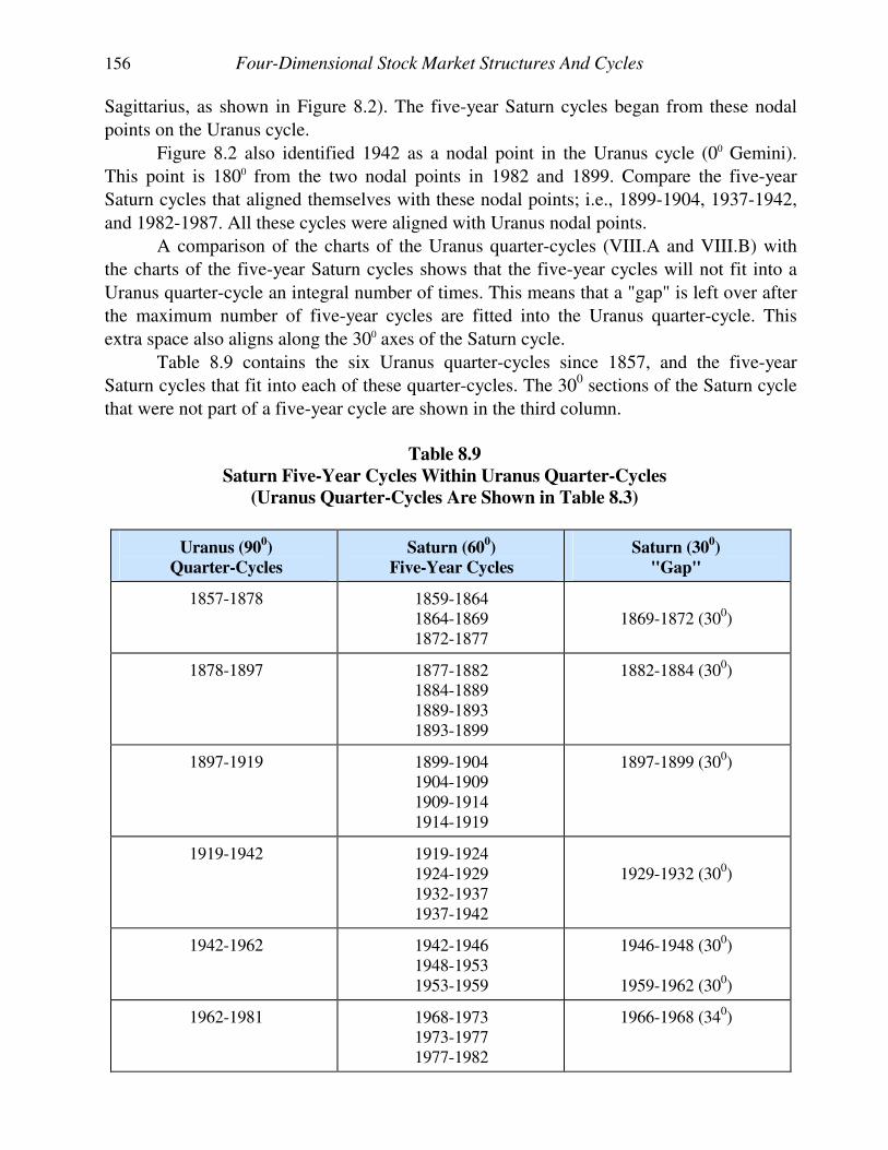
156 Four-Dimensional Stock Market Structures And Cycles
Sagittarius, as shown in Figure 8.2). The five-year Saturn cycles began from these nodal
points on the Uranus cycle.
Figure 8.2 also identified 1942 as a nodal point in the Uranus cycle (00 Gemini).
This point is 1800 from the two nodal points in 1982 and 1899. Compare the five-year
Saturn cycles that aligned themselves with these nodal points; i.e., 1899-1904, 1937-1942,
and 1982-1987. All these cycles were aligned with Uranus nodal points.
A comparison of the charts of the Uranus quarter-cycles (VIII.A and VIII.B) with
the charts of the five-year Saturn cycles shows that the five-year cycles will not fit into a
Uranus quarter-cycle an integral number of times. This means that a "gap" is left over after
the maximum number of five-year cycles are fitted into the Uranus quarter-cycle. This
extra space also aligns along the 300 axes of the Saturn cycle.
Table 8.9 contains the six Uranus quarter-cycles since 1857, and the five-year
Saturn cycles that fit into each of these quarter-cycles. The 300 sections of the Saturn cycle
that were not part of a five-year cycle are shown in the third column.
Table 8.9
Saturn Five-Year Cycles Within Uranus Quarter-Cycles
(Uranus Quarter-Cycles Are Shown in Table 8.3)
Uranus (900)
Quarter-Cycles
Saturn (600)
Five-Year Cycles
Saturn (300)
"Gap"
1857-1878 1859-1864 1864-1869 1872-1877
1869-1872 (300)
1878-1897 1877-1882 1884-1889 1889-1893 1893-1899
1882-1884 (300)
1897-1919 1899-1904 1904-1909 1909-1914 1914-1919
1897-1899 (300)
1919-1942 1919-1924 1924-1929 1932-1937 1937-1942
1929-1932 (300)
1942-1962 1942-1946 1948-1953 1953-1959
1946-1948 (300) 1959-1962 (300)
1962-1981 1968-1973 1973-1977 1977-1982
1966-1968 (340)
Planetary Cycles 157
For example, the Uranus quarter-cycle from 1857 to 1878 contained three
completed five-year cycles; 1859-1864, 1864-1869, 1872-1877, as shown on Chart VIII.K.
The "gap" was between 1869 and 1872. During this time, Saturn moved 300, from 170
Sagittarius to 170 Capricorn. Similarly, the Uranus quarter-cycle from 1897 to 1919,
contained four completed five-year cycles; 1899-1904, 1904-1909, 1909-1914, 1914-1919,
as shown on Chart VIII.L. The "gap" was from 1897 to 1899. During this time Saturn
moved 300, from 260 Scorpio to 260 Sagittarius.
The Uranus quarter-cycle from 1919 to 1942 contained four completed five-year
cycles; 1919-1924, 1924-1929, 1932-1937, 1937-1942, as shown on Charts VIII.L and
VIII.M. The "gap" was the crash between 1929 and 1932. During this time Saturn again
moved 300, from 00 Capricorn to 00 Aquarius.
Because the price-time action within the 1949-1966 square traversed it diagonally,
effectively defining the increasing energy level, prices experienced a strong upward force
during this period. This made it difficult to clearly identify the smaller cycles, including the
five-year cycle.
JUPITER-SATURN CYCLE AND STOCK MARKET CORRELATION
Jupiter and Saturn conjoin every twenty years. Therefore, each 300 movement of
Jupiter relative to Saturn averages twenty months. Each conjunction moves about 2400
relative to the fixed stars from the previous conjunction. This means that every sixty years
the third conjunction between these two planets occurs in approximately the same position
in the heavens. During this sixty-year period Uranus completes three quarter-cycles, or
2700.
When a conjunction occurs at the same longitude and latitude as a previous
conjunction, it is known as a "first order conjunction". This period is 60 years for the
Jupiter-Saturn cycle. The 60-year cycle was one listed by W.D. Gann in his Master Course
For Stocks as a major cycle.
Financial astrologers have used the Jupiter-Saturn cycle for years to try to predict
financial market prices and is the basis of the decennial period (10 Year) identified by
Edgar Lawrence Smith, W.D. Gann, et. al.81
A complete record of the New York Stock Exchange from 1790 to 1993 can be
charted. When these charts are divided into twenty-year periods, an easy comparison of the
stock market during separate Jupiter-Saturn cycles is possible. Compare similar points on
these charts to see for yourself if there is anything to the twenty-year stock market period.82
81 W.D. Gann produced and made available to the public "Annual Forecasts", which he sold for large sums of money. These forecasts were based upon the decennial period. Appendix C contains an example of how W.D. Gann made his annual forecasts.
82 Appendix D contains a discussion of the twenty-year presidential cycle. Briefly stated, the president elected every 20 years, during the Jupiter-Saturn conjunction, dies in office.
158 Four-Dimensional Stock Market Structures And Cycles
Long-term wheat data allows the reader to extend this analysis back to the year
1290. Along with the 200-year rhythm, 60-year spikes in price corresponding with the
Jupiter-Saturn cycle are clearly present in the wheat market. On a smaller magnitude, a ten-
year rhythm can also be clearly seen on that chart.
20-MONTH JUPITER-SATURN HARMONIC AND STOCK MARKET CYCLES
THERE IS A CYCLE OF ALTERNATING ADVANCING AND
DECLINING PRICES IN THE STOCK MARKET CORRELATED
WITH 150 MOTIONS OF THE JUPITER-SATURN CYCLE. THESE
CYCLES AVERAGE 20 MONTHS FROM BOTTOM-TO-BOTTOM OR
TOP-TO-TOP.
Since this cycle only defines a ten-month trend, a smaller time frame will be used to
study its effects in the stock market. Chart VIII.O shows the DJIA from 1/1980 to 6/1993
with the 150 axes of the Jupiter-Saturn cycle drawn in. There are two sets of vertical lines
on this chart. The dotted lines define the 150 axes. The solid lines also define 150 axes,
however they are spaced to identify the sympathetic resonance between the Jupiter-Saturn
cycle and the harmonics of the larger Saturn-Uranus cycle. In other words, the solid
vertical lines on Chart VIII.O are spaced either 300 or 450 apart, depending upon which of
these two divisions corresponds more closely with the 150 axes of the larger Saturn-Uranus
cycle shown on Chart VIII.I. Compare these two charts and see how closely the harmonics
of these two planetary cycles correspond.
Chart VIII.O shows that there are sometimes two and sometimes three divisions of
the larger Saturn-Uranus cycle by the smaller Jupiter-Saturn cycle. That is, the Saturn-
Uranus 150 harmonic sometimes corresponds with 300 on the Jupiter-Saturn cycle and
sometimes with 450. Whichever division is taking place, the two cycles are synchronous. It
is critical that this relationship is understood, because this is the mechanism used to
determine the subdivisions of the cycles. A CYCLE IS MORE PRONOUNCED IF IT
IS REINFORCED BY THE HARMONICS OF ANOTHER CYCLE.83 The solid
vertical lines on Chart VIII.O show where these two major cycles reinforce each other,
effectively identifying key turning points in the stock market. This concept of subdivision
of larger cycles by the smaller cycles is expanded later in this lesson.
The exact data for the Jupiter-Saturn cycle are contained in Tables 8.10.a and
8.10.b. Having the data in table format allows the reader to identify the precise location of
the Jupiter-Saturn cycle when turning points in the DJIA occurred. As in previous tables,
the location of the Jupiter-Saturn cycle is given at the beginning and end of the related
advance or decline in the stock market. The change in relative position of the Jupiter-
Saturn cycle, during the advance or decline, is included in the last column. Even when the
83 Technical Reference: Fundamentals of Physics – Extended, P. 409-412.
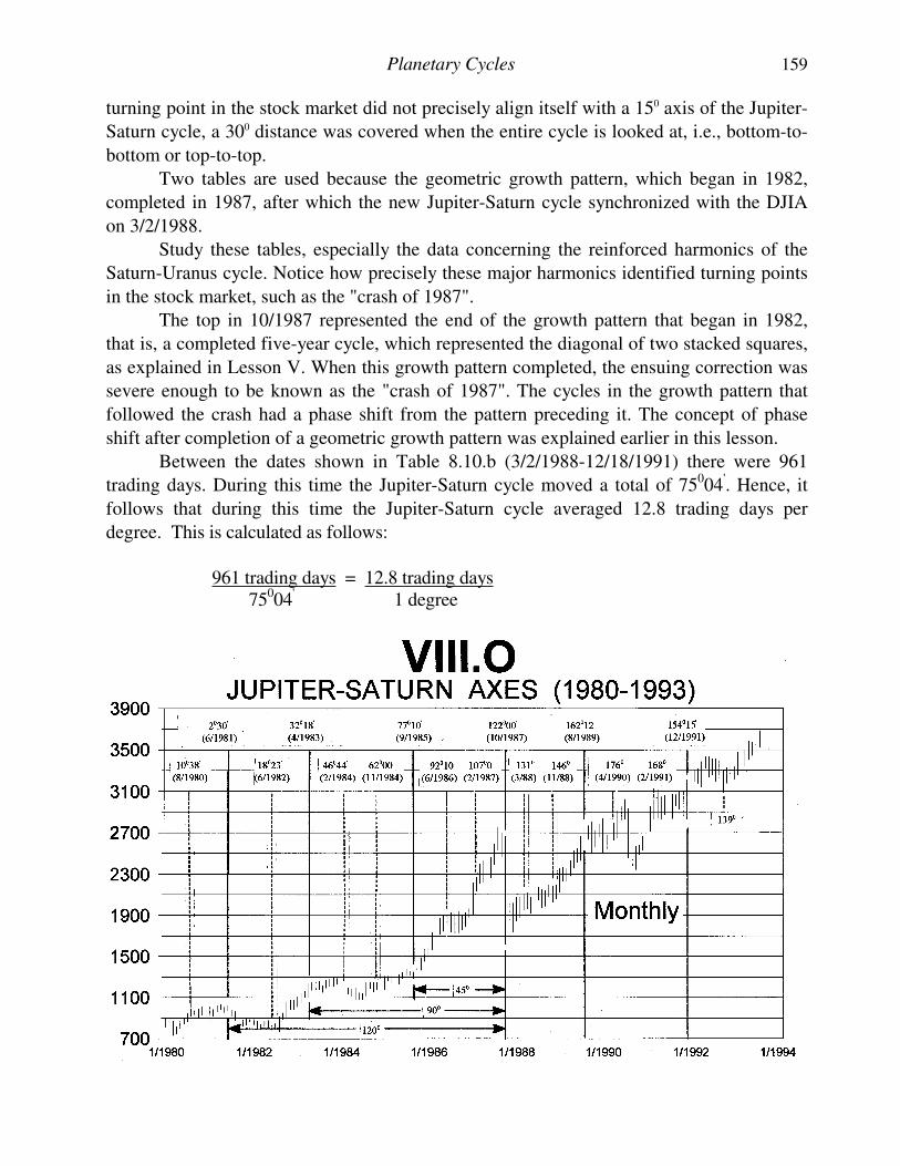
Planetary Cycles 159
turning point in the stock market did not precisely align itself with a 150 axis of the Jupiter-
Saturn cycle, a 300 distance was covered when the entire cycle is looked at, i.e., bottom-to-
bottom or top-to-top.
Two tables are used because the geometric growth pattern, which began in 1982,
completed in 1987, after which the new Jupiter-Saturn cycle synchronized with the DJIA
on 3/2/1988.
Study these tables, especially the data concerning the reinforced harmonics of the
Saturn-Uranus cycle. Notice how precisely these major harmonics identified turning points
in the stock market, such as the "crash of 1987".
The top in 10/1987 represented the end of the growth pattern that began in 1982,
that is, a completed five-year cycle, which represented the diagonal of two stacked squares,
as explained in Lesson V. When this growth pattern completed, the ensuing correction was
severe enough to be known as the "crash of 1987". The cycles in the growth pattern that
followed the crash had a phase shift from the pattern preceding it. The concept of phase
shift after completion of a geometric growth pattern was explained earlier in this lesson.
Between the dates shown in Table 8.10.b (3/2/1988-12/18/1991) there were 961
trading days. During this time the Jupiter-Saturn cycle moved a total of 75004'. Hence, it
follows that during this time the Jupiter-Saturn cycle averaged 12.8 trading days per
degree. This is calculated as follows:
961 trading days = 12.8 trading days 75004' 1 degree
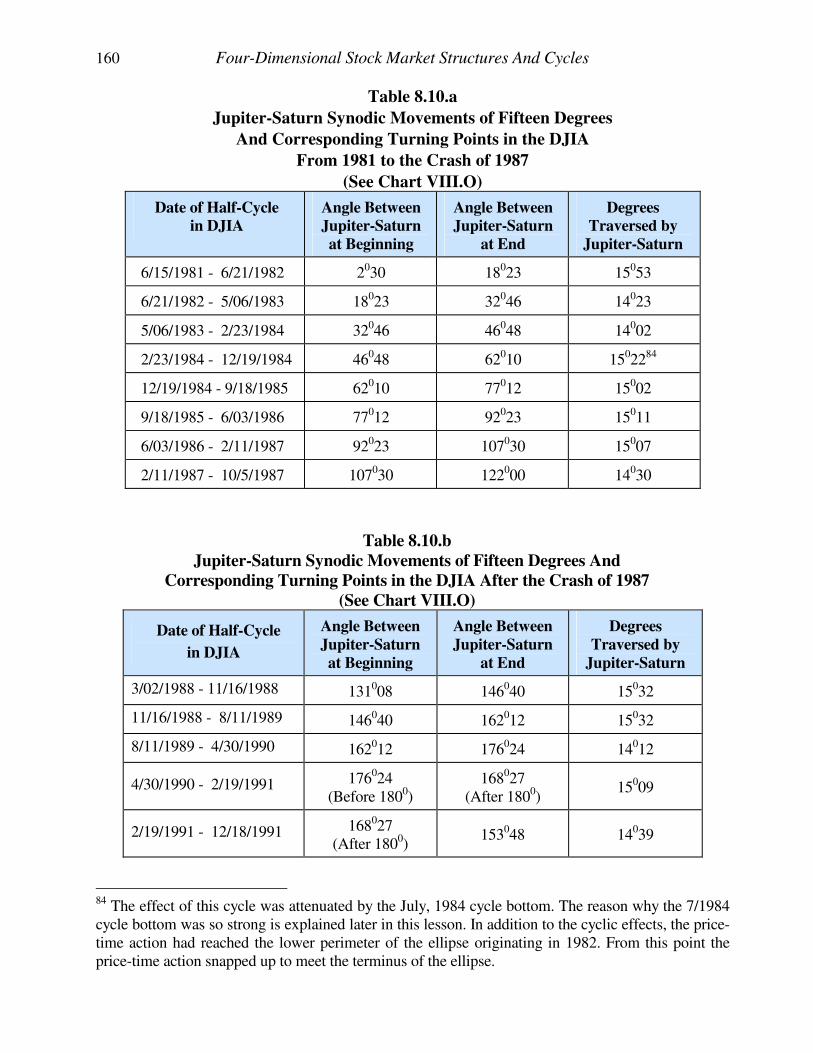
160 Four-Dimensional Stock Market Structures And Cycles
Table 8.10.a
Jupiter-Saturn Synodic Movements of Fifteen Degrees
And Corresponding Turning Points in the DJIA
From 1981 to the Crash of 1987
(See Chart VIII.O)
Date of Half-Cycle
in DJIA
Angle Between
Jupiter-Saturn
at Beginning
Angle Between
Jupiter-Saturn
at End
Degrees
Traversed by
Jupiter-Saturn
6/15/1981 - 6/21/1982 2030 18023 15053
6/21/1982 - 5/06/1983 18023 32046 14023
5/06/1983 - 2/23/1984 32046 46048 14002
2/23/1984 - 12/19/1984 46048 62010 1502284
12/19/1984 - 9/18/1985 62010 77012 15002
9/18/1985 - 6/03/1986 77012 92023 15011
6/03/1986 - 2/11/1987 92023 107030 15007
2/11/1987 - 10/5/1987 107030 122000 14030
Table 8.10.b
Jupiter-Saturn Synodic Movements of Fifteen Degrees And
Corresponding Turning Points in the DJIA After the Crash of 1987
(See Chart VIII.O)
Date of Half-Cycle
in DJIA
Angle Between
Jupiter-Saturn
at Beginning
Angle Between
Jupiter-Saturn
at End
Degrees
Traversed by
Jupiter-Saturn
3/02/1988 - 11/16/1988 131008 146040 15032
11/16/1988 - 8/11/1989 146040 162012 15032
8/11/1989 - 4/30/1990 162012 176024 14012
4/30/1990 - 2/19/1991 176024 (Before 1800)
168027 (After 1800)
15009
2/19/1991 - 12/18/1991 168027 (After 1800)
153048 14039
84 The effect of this cycle was attenuated by the July, 1984 cycle bottom. The reason why the 7/1984 cycle bottom was so strong is explained later in this lesson. In addition to the cyclic effects, the price-time action had reached the lower perimeter of the ellipse originating in 1982. From this point the price-time action snapped up to meet the terminus of the ellipse.
Planetary Cycles 161
Since the actual DJIA turning points in Tables 8.10.a and 8.10.b rarely deviated
from the Jupiter-Saturn 150 axes by more than one-half degree, this represented an average
error of 6-7 trading days. This error must be viewed in the context that it is measured
within a large cycle with an average trend of ten months. A deviation of six trading days in
a cycle lasting ten months represents an error of less than 3%. For comparison, a 3% error
in an eight-week cycle is about one trading day. The error is even less than 3% when measurements are made top-to-top or bottom-to-bottom. The 3% value represents the worst-case scenario of top-to-bottom or bottom-to-top, defined by the 150 axes.
JUPITER-URANUS CYCLE AND STOCK MARKET CORRELATION
The Jupiter-Uranus cycle completes one synodic period every fourteen years. This
means that Jupiter-Uranus moves 1800 as Uranus moves 300, relative to the fixed stars,
completing a seven-year cycle. As with other cycles, the Jupiter-Uranus cycle has axes
every fifteen degrees, which last on average seven months.
FIFTEEN-DEGREE SECTIONS OF THE JUPITER-URANUS CYCLE
DEFINE THE SEVEN-MONTH STOCK MARKET CYCLE.
As with the Jupiter-Saturn cycle, a smaller time frame will be used to study the
effects of this cycle in the DJIA because it has a smaller period. For example, Chart VIII.P
shows the DJIA between 1/1980 and 6/1993. The vertical lines show the 300 harmonics of
the Jupiter-Uranus cycle.
Just as the harmonics of the Jupiter-Saturn cycle correspond with the harmonics of
the Saturn-Uranus cycle, the Jupiter-Uranus harmonics correspond with both the Saturn-
Uranus and the Jupiter-Saturn harmonics. Hence, all three of these major cycles reinforce
each other. Compare the 150 harmonics of the Saturn-Uranus cycle on Chart VIII.I with the
Jupiter-Uranus cycles shown on Chart VIII.P. Also, compare the Jupiter-Saturn harmonics
on Chart VIII.O with those of Jupiter-Uranus shown on Chart VIII.P. These three charts
show how the major cycles synchronize along their 150 axes.
The fifteen-degree axes of the Jupiter-Uranus cycle and corresponding turning
points in the DJIA between March, 1980 and the crash of October, 1987 are listed in Table
8.11.a. The data after October, 1987 are included in Table 8.11.b.
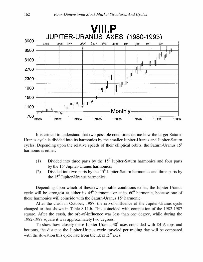
162 Four-Dimensional Stock Market Structures And Cycles
It is critical to understand that two possible conditions define how the larger Saturn-
Uranus cycle is divided into its harmonics by the smaller Jupiter-Uranus and Jupiter-Saturn
cycles. Depending upon the relative speeds of their elliptical orbits, the Saturn-Uranus 150
harmonic is either:
(1) Divided into three parts by the 150 Jupiter-Saturn harmonics and four parts
by the 150 Jupiter-Uranus harmonics.
(2) Divided into two parts by the 150 Jupiter-Saturn harmonics and three parts by
the 150 Jupiter-Uranus harmonics.
Depending upon which of these two possible conditions exists, the Jupiter-Uranus
cycle will be strongest at either its 450 harmonic or at its 600 harmonic, because one of
these harmonics will coincide with the Saturn-Uranus 150 harmonic.
After the crash in October, 1987, the orb-of-influence of the Jupiter-Uranus cycle
changed to that shown in Table 8.11.b. This coincided with completion of the 1982-1987
square. After the crash, the orb-of-influence was less than one degree, while during the
1982-1987 square it was approximately two degrees.
To show how closely these Jupiter-Uranus 300 axes coincided with DJIA tops and
bottoms, the distance the Jupiter-Uranus cycle traveled per trading day will be compared
with the deviation this cycle had from the ideal 150 axes.
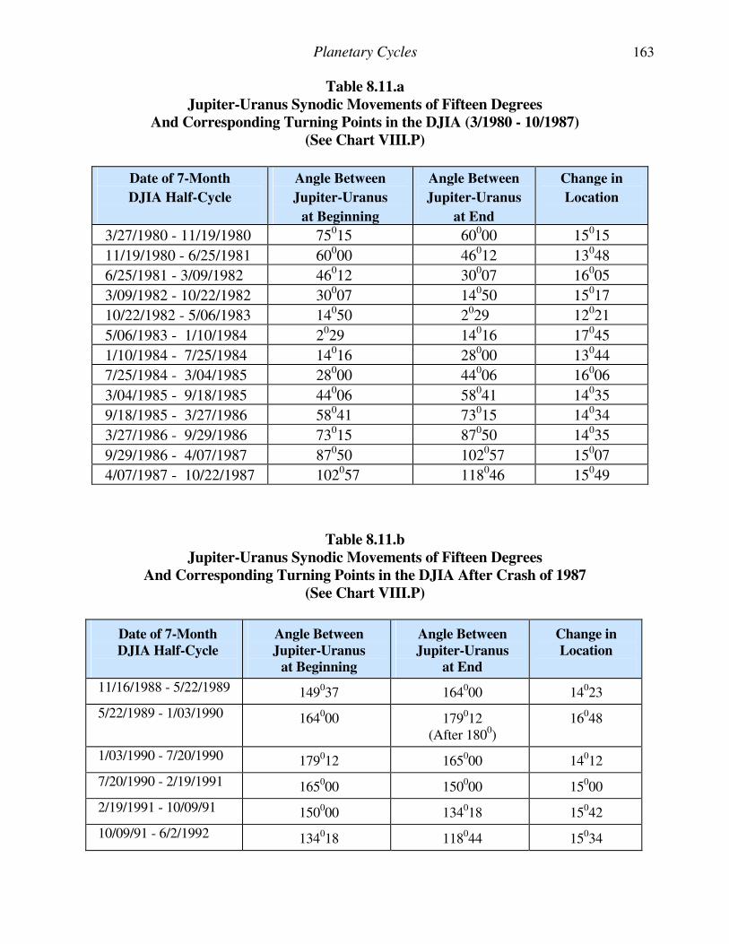
Planetary Cycles 163
Table 8.11.a
Jupiter-Uranus Synodic Movements of Fifteen Degrees
And Corresponding Turning Points in the DJIA (3/1980 - 10/1987)
(See Chart VIII.P)
Date of 7-Month
DJIA Half-Cycle
Angle Between
Jupiter-Uranus
at Beginning
Angle Between
Jupiter-Uranus
at End
Change in
Location
3/27/1980 - 11/19/1980 75015 60000 15015
11/19/1980 - 6/25/1981 60000 46012 13048
6/25/1981 - 3/09/1982 46012 30007 16005
3/09/1982 - 10/22/1982 30007 14050 15017
10/22/1982 - 5/06/1983 14050 2029 12021
5/06/1983 - 1/10/1984 2029 14016 17045
1/10/1984 - 7/25/1984 14016 28000 13044
7/25/1984 - 3/04/1985 28000 44006 16006
3/04/1985 - 9/18/1985 44006 58041 14035
9/18/1985 - 3/27/1986 58041 73015 14034
3/27/1986 - 9/29/1986 73015 87050 14035
9/29/1986 - 4/07/1987 87050 102057 15007
4/07/1987 - 10/22/1987 102057 118046 15049
Table 8.11.b
Jupiter-Uranus Synodic Movements of Fifteen Degrees
And Corresponding Turning Points in the DJIA After Crash of 1987
(See Chart VIII.P)
Date of 7-Month
DJIA Half-Cycle
Angle Between
Jupiter-Uranus
at Beginning
Angle Between
Jupiter-Uranus
at End
Change in
Location
11/16/1988 - 5/22/1989 149037 164000 14023
5/22/1989 - 1/03/1990 164000 179012 (After 1800)
16048
1/03/1990 - 7/20/1990 179012 165000 14012
7/20/1990 - 2/19/1991 165000 150000 15000
2/19/1991 - 10/09/91 150000 134018 15042
10/09/91 - 6/2/1992 134018 118044 15034
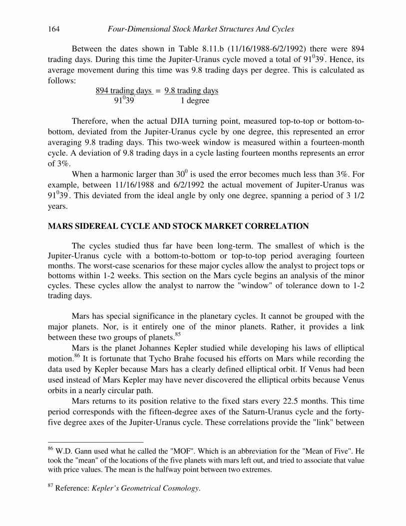
164 Four-Dimensional Stock Market Structures And Cycles
Between the dates shown in Table 8.11.b (11/16/1988-6/2/1992) there were 894
trading days. During this time the Jupiter-Uranus cycle moved a total of 91039'. Hence, its
average movement during this time was 9.8 trading days per degree. This is calculated as
follows: 894 trading days = 9.8 trading days 91039' 1 degree
Therefore, when the actual DJIA turning point, measured top-to-top or bottom-to-
bottom, deviated from the Jupiter-Uranus cycle by one degree, this represented an error
averaging 9.8 trading days. This two-week window is measured within a fourteen-month
cycle. A deviation of 9.8 trading days in a cycle lasting fourteen months represents an error
of 3%.
When a harmonic larger than 300 is used the error becomes much less than 3%. For
example, between 11/16/1988 and 6/2/1992 the actual movement of Jupiter-Uranus was
91039'. This deviated from the ideal angle by only one degree, spanning a period of 3 1/2
years.
MARS SIDEREAL CYCLE AND STOCK MARKET CORRELATION The cycles studied thus far have been long-term. The smallest of which is the Jupiter-Uranus cycle with a bottom-to-bottom or top-to-top period averaging fourteen months. The worst-case scenarios for these major cycles allow the analyst to project tops or bottoms within 1-2 weeks. This section on the Mars cycle begins an analysis of the minor cycles. These cycles allow the analyst to narrow the "window" of tolerance down to 1-2 trading days.
Mars has special significance in the planetary cycles. It cannot be grouped with the
major planets. Nor, is it entirely one of the minor planets. Rather, it provides a link
between these two groups of planets.85
Mars is the planet Johannes Kepler studied while developing his laws of elliptical
motion.86 It is fortunate that Tycho Brahe focused his efforts on Mars while recording the
data used by Kepler because Mars has a clearly defined elliptical orbit. If Venus had been
used instead of Mars Kepler may have never discovered the elliptical orbits because Venus
orbits in a nearly circular path.
Mars returns to its position relative to the fixed stars every 22.5 months. This time
period corresponds with the fifteen-degree axes of the Saturn-Uranus cycle and the forty-
five degree axes of the Jupiter-Uranus cycle. These correlations provide the "link" between
86 W.D. Gann used what he called the "MOF". Which is an abbreviation for the "Mean of Five". He took the "mean" of the locations of the five planets with mars left out, and tried to associate that value with price values. The mean is the halfway point between two extremes.
87 Reference: Kepler’s Geometrical Cosmology.
Planetary Cycles 165
the harmonics of the major planets and the periods of the minor planets, as shown in
Figures 6.2 and 6.3.
The previous section on the Jupiter-Uranus cycle measured the difference between
the date of the actual DJIA top or bottom and the date the Jupiter-Uranus axes were
reached. Several of these deviations were caused by the synchrony that exists between the
Mars trine and the Jupiter-Uranus 150 harmonic. The DJIA bottoms and tops deviated from
the ideal Jupiter-Uranus 150 axes when the Mars trine and the Jupiter-Uranus axes were not
perfectly aligned.
Two critical areas of the Mars cycle deserve special attention. They are located sixty
degrees apart at 190 Virgo and 190 Scorpio. These two points often identify bottom-to-top or
top-to-bottom swings in the stock market. The reason why these two areas are so important is
explained in the next section on the musical twelfth of the Mars cycle. In short, this is where
the Mars cycle shifts between two trines (1200) when it becomes asynchronous with the 150
Jupiter-Uranus harmonic.
Chart VIII.Q shows a period of twenty-seven years with these two critical areas of the
Mars cycle identified. The data for the Scorpio turning points from 5/1969 to 11/1991 are
listed in Table 8.12.a, and those for 190 of Virgo are listed in Table 8.12.b. Chart VIII.Q
shows how almost every major turning point between 1965 and 1992 coincided with these
two locations in the Mars cycle.
Recently, the dates 3/27/1980, 1/10/1984, and 10/2/1987 are all well-known turning
points in the DJIA that corresponded with the location of 190 Virgo in the Mars cycle.
Since Mars moves 3600 in approximately 465 trading days, it averages 1.3 trading
days per degree. Therefore, it averages 30 motion in four trading days. Three degrees on
either side of 190 is 160-220, which encompasses most of the items in Tables 8.12.a and
8.12.b. This + 30 range provides a window of tolerance of + 4 trading days.
When calculating the error it must be realized that many of the turning points listed
in Tables 8.12.a and 8.12.b were not sharply defined. Many times the actual DJIA high or
low did not occur very far from the day the ideal Mars angle was crossed.
OCTAVES (1/2; 1/4; 1/8) OF THE MARS CYCLE AND THE STOCK MARKET
Mars is synchronized with the period of Mercury in the ratio of eight to one,
defining the triple octave. When Mars completes one cycle, Mercury completes eight. Or,
THE COMPLETE MERCURY CYCLE IS SYNCHRONIZED WITH
THE 450 HARMONIC OF THE MARS CYCLE.
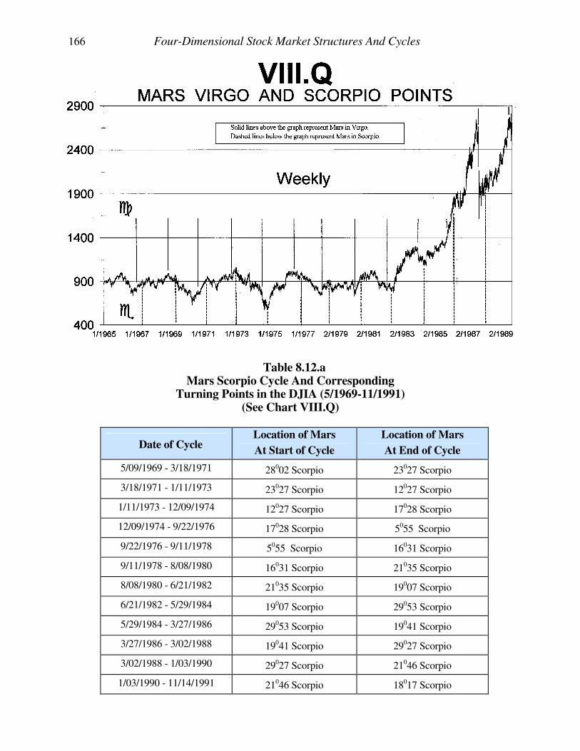
166 Four-Dimensional Stock Market Structures And Cycles
Table 8.12.a Mars Scorpio Cycle And Corresponding Turning Points in the DJIA (5/1969-11/1991) (See Chart VIII.Q)
Date of Cycle Location of Mars
At Start of Cycle
Location of Mars
At End of Cycle
5/09/1969 - 3/18/1971 28002 Scorpio 23027 Scorpio
3/18/1971 - 1/11/1973 23027 Scorpio 12027 Scorpio
1/11/1973 - 12/09/1974 12027 Scorpio 17028 Scorpio
12/09/1974 - 9/22/1976 17028 Scorpio 5055 Scorpio
9/22/1976 - 9/11/1978 5055 Scorpio 16031 Scorpio
9/11/1978 - 8/08/1980 16031 Scorpio 21035 Scorpio
8/08/1980 - 6/21/1982 21035 Scorpio 19007 Scorpio
6/21/1982 - 5/29/1984 19007 Scorpio 29053 Scorpio
5/29/1984 - 3/27/1986 29053 Scorpio 19041 Scorpio
3/27/1986 - 3/02/1988 19041 Scorpio 29027 Scorpio
3/02/1988 - 1/03/1990 29027 Scorpio 21046 Scorpio
1/03/1990 - 11/14/1991 21046 Scorpio 18017 Scorpio
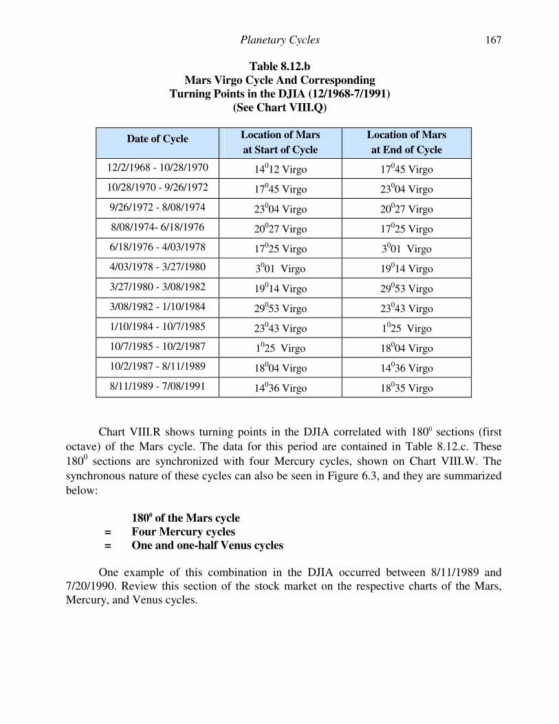
Planetary Cycles 167
Table 8.12.b
Mars Virgo Cycle And Corresponding
Turning Points in the DJIA (12/1968-7/1991)
(See Chart VIII.Q)
Date of Cycle Location of Mars
at Start of Cycle
Location of Mars
at End of Cycle
12/2/1968 - 10/28/1970 14012 Virgo 17045 Virgo
10/28/1970 - 9/26/1972 17045 Virgo 23004 Virgo
9/26/1972 - 8/08/1974 23004 Virgo 20027 Virgo
8/08/1974- 6/18/1976 20027 Virgo 17025 Virgo
6/18/1976 - 4/03/1978 17025 Virgo 3001 Virgo
4/03/1978 - 3/27/1980 3001 Virgo 19014 Virgo
3/27/1980 - 3/08/1982 19014 Virgo 29053 Virgo
3/08/1982 - 1/10/1984 29053 Virgo 23043 Virgo
1/10/1984 - 10/7/1985 23043 Virgo 1025 Virgo
10/7/1985 - 10/2/1987 1025 Virgo 18004 Virgo
10/2/1987 - 8/11/1989 18004 Virgo 14036 Virgo
8/11/1989 - 7/08/1991 14036 Virgo 18035 Virgo
Chart VIII.R shows turning points in the DJIA correlated with 1800 sections (first
octave) of the Mars cycle. The data for this period are contained in Table 8.12.c. These
1800 sections are synchronized with four Mercury cycles, shown on Chart VIII.W. The
synchronous nature of these cycles can also be seen in Figure 6.3, and they are summarized
below: 1800 of the Mars cycle
= Four Mercury cycles
= One and one-half Venus cycles One example of this combination in the DJIA occurred between 8/11/1989 and 7/20/1990. Review this section of the stock market on the respective charts of the Mars, Mercury, and Venus cycles.
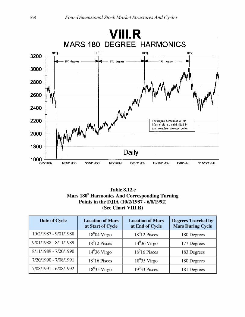
168 Four-Dimensional Stock Market Structures And Cycles
Table 8.12.c
Mars 1800 Harmonics And Corresponding Turning
Points in the DJIA (10/2/1987 - 6/8/1992)
(See Chart VIII.R)
Date of Cycle Location of Mars
at Start of Cycle
Location of Mars
at End of Cycle
Degrees Traveled by
Mars During Cycle
10/2/1987 - 9/01/1988 18004 Virgo 18012 Pisces 180 Degrees
9/01/1988 - 8/11/1989 18012 Pisces 14036 Virgo 177 Degrees
8/11/1989 - 7/20/1990 14036 Virgo 18016 Pisces 183 Degrees
7/20/1990 - 7/08/1991 18016 Pisces 18035 Virgo 180 Degrees
7/08/1991 - 6/08/1992 18035 Virgo 19033 Pisces 181 Degrees
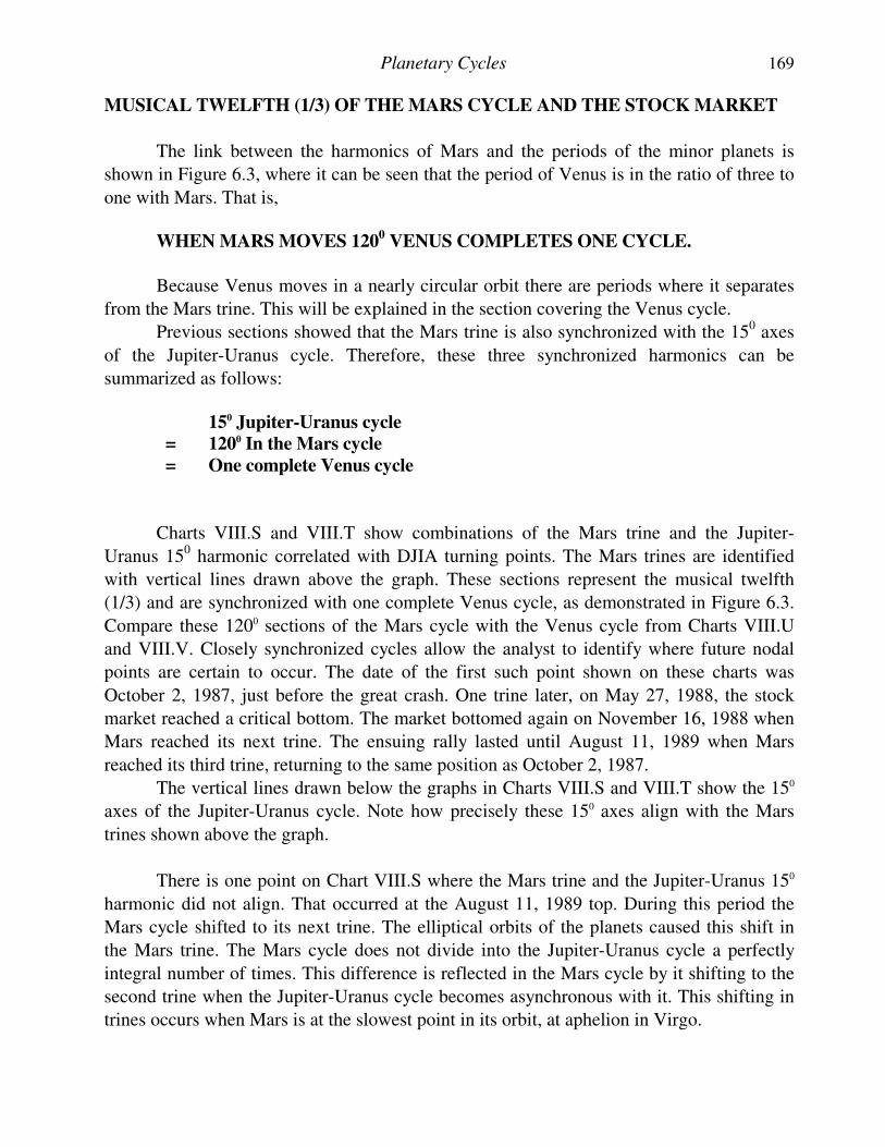
Planetary Cycles 169
MUSICAL TWELFTH (1/3) OF THE MARS CYCLE AND THE STOCK MARKET
The link between the harmonics of Mars and the periods of the minor planets is
shown in Figure 6.3, where it can be seen that the period of Venus is in the ratio of three to
one with Mars. That is, WHEN MARS MOVES 120
0 VENUS COMPLETES ONE CYCLE.
Because Venus moves in a nearly circular orbit there are periods where it separates
from the Mars trine. This will be explained in the section covering the Venus cycle.
Previous sections showed that the Mars trine is also synchronized with the 150 axes
of the Jupiter-Uranus cycle. Therefore, these three synchronized harmonics can be
summarized as follows:
150 Jupiter-Uranus cycle
= 1200 In the Mars cycle
= One complete Venus cycle
Charts VIII.S and VIII.T show combinations of the Mars trine and the Jupiter-
Uranus 150 harmonic correlated with DJIA turning points. The Mars trines are identified
with vertical lines drawn above the graph. These sections represent the musical twelfth
(1/3) and are synchronized with one complete Venus cycle, as demonstrated in Figure 6.3.
Compare these 1200 sections of the Mars cycle with the Venus cycle from Charts VIII.U
and VIII.V. Closely synchronized cycles allow the analyst to identify where future nodal
points are certain to occur. The date of the first such point shown on these charts was
October 2, 1987, just before the great crash. One trine later, on May 27, 1988, the stock
market reached a critical bottom. The market bottomed again on November 16, 1988 when
Mars reached its next trine. The ensuing rally lasted until August 11, 1989 when Mars
reached its third trine, returning to the same position as October 2, 1987.
The vertical lines drawn below the graphs in Charts VIII.S and VIII.T show the 150
axes of the Jupiter-Uranus cycle. Note how precisely these 150 axes align with the Mars
trines shown above the graph.
There is one point on Chart VIII.S where the Mars trine and the Jupiter-Uranus 150
harmonic did not align. That occurred at the August 11, 1989 top. During this period the
Mars cycle shifted to its next trine. The elliptical orbits of the planets caused this shift in
the Mars trine. The Mars cycle does not divide into the Jupiter-Uranus cycle a perfectly
integral number of times. This difference is reflected in the Mars cycle by it shifting to the
second trine when the Jupiter-Uranus cycle becomes asynchronous with it. This shifting in
trines occurs when Mars is at the slowest point in its orbit, at aphelion in Virgo.
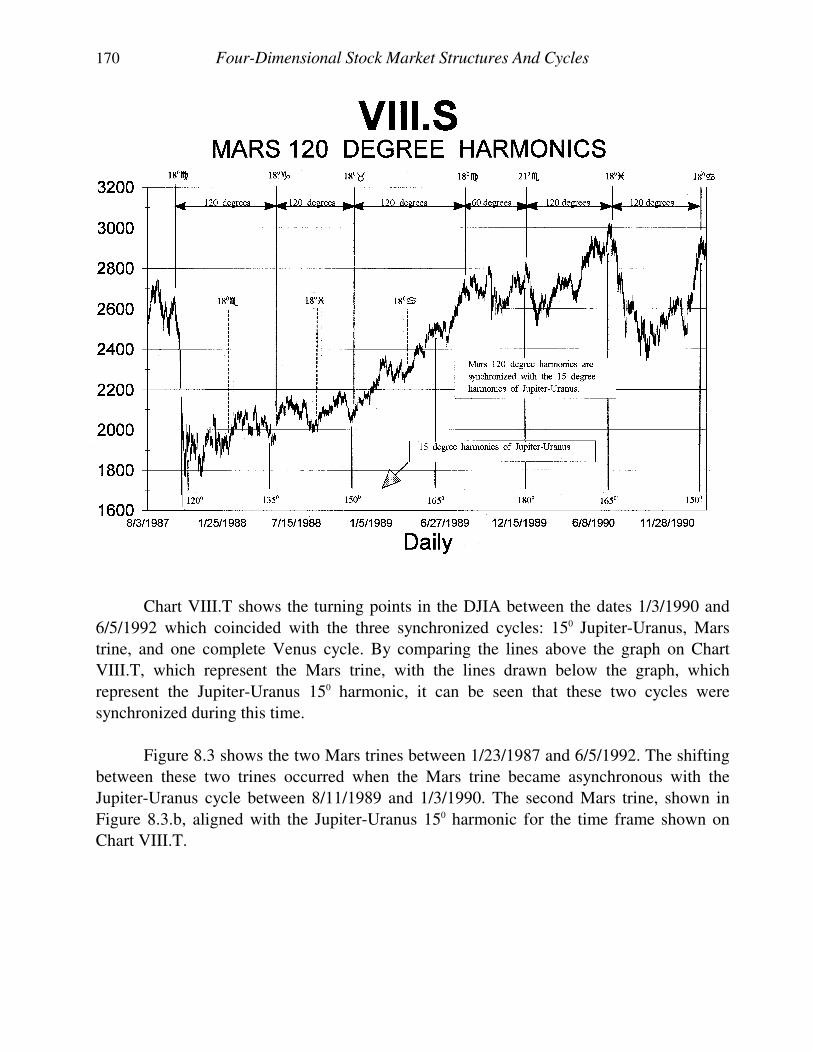
170 Four-Dimensional Stock Market Structures And Cycles
Chart VIII.T shows the turning points in the DJIA between the dates 1/3/1990 and
6/5/1992 which coincided with the three synchronized cycles: 150 Jupiter-Uranus, Mars
trine, and one complete Venus cycle. By comparing the lines above the graph on Chart
VIII.T, which represent the Mars trine, with the lines drawn below the graph, which
represent the Jupiter-Uranus 150 harmonic, it can be seen that these two cycles were
synchronized during this time.
Figure 8.3 shows the two Mars trines between 1/23/1987 and 6/5/1992. The shifting
between these two trines occurred when the Mars trine became asynchronous with the
Jupiter-Uranus cycle between 8/11/1989 and 1/3/1990. The second Mars trine, shown in
Figure 8.3.b, aligned with the Jupiter-Uranus 150 harmonic for the time frame shown on
Chart VIII.T.
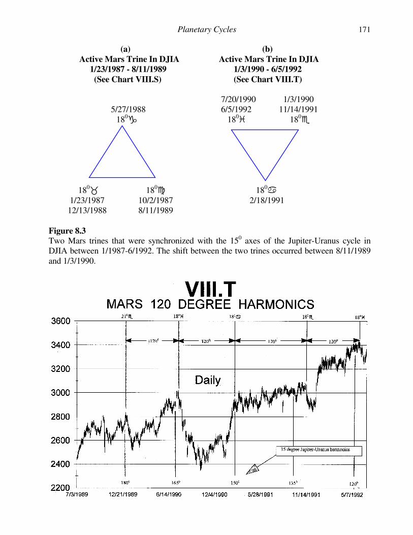
Planetary Cycles 171
(a) (b)
Active Mars Trine In DJIA Active Mars Trine In DJIA
1/23/1987 - 8/11/1989 1/3/1990 - 6/5/1992
(See Chart VIII.S) (See Chart VIII.T) 7/20/1990 1/3/1990 5/27/1988 6/5/1992 11/14/1991 180 180� 180� 180� 180� 180� 1/23/1987 10/2/1987 2/18/1991 12/13/1988 8/11/1989 Figure 8.3 Two Mars trines that were synchronized with the 150 axes of the Jupiter-Uranus cycle in DJIA between 1/1987-6/1992. The shift between the two trines occurred between 8/11/1989 and 1/3/1990.
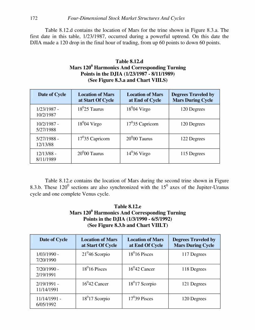
172 Four-Dimensional Stock Market Structures And Cycles
Table 8.12.d contains the location of Mars for the trine shown in Figure 8.3.a. The first date in this table, 1/23/1987, occurred during a powerful uptrend. On this date the DJIA made a 120 drop in the final hour of trading, from up 60 points to down 60 points.
Table 8.12.d
Mars 1200 Harmonics And Corresponding Turning
Points in the DJIA (1/23/1987 - 8/11/1989)
(See Figure 8.3.a and Chart VIII.S)
Date of Cycle Location of Mars
at Start Of Cycle
Location of Mars
at End of Cycle
Degrees Traveled by
Mars During Cycle
1/23/1987 - 10/2/1987
18025 Taurus 18004 Virgo 120 Degrees
10/2/1987 - 5/27/1988
18004 Virgo 17035 Capricorn 120 Degrees
5/27/1988 - 12/13/88
17035 Capricorn 20000 Taurus 122 Degrees
12/13/88 - 8/11/1989
20000 Taurus 14036 Virgo 115 Degrees
Table 8.12.e contains the location of Mars during the second trine shown in Figure
8.3.b. These 1200 sections are also synchronized with the 150 axes of the Jupiter-Uranus
cycle and one complete Venus cycle. Table 8.12.e
Mars 1200 Harmonics And Corresponding Turning
Points in the DJIA (1/3/1990 - 6/5/1992)
(See Figure 8.3.b and Chart VIII.T)
Date of Cycle Location of Mars
at Start Of Cycle
Location of Mars
at End Of Cycle
Degrees Traveled by
Mars During Cycle
1/03/1990 - 7/20/1990
21046 Scorpio 18016 Pisces 117 Degrees
7/20/1990 - 2/19/1991
18016 Pisces 16042 Cancer 118 Degrees
2/19/1991 - 11/14/1991
16042 Cancer 18017 Scorpio 121 Degrees
11/14/1991 - 6/05/1992
18017 Scorpio 17039 Pisces 120 Degrees
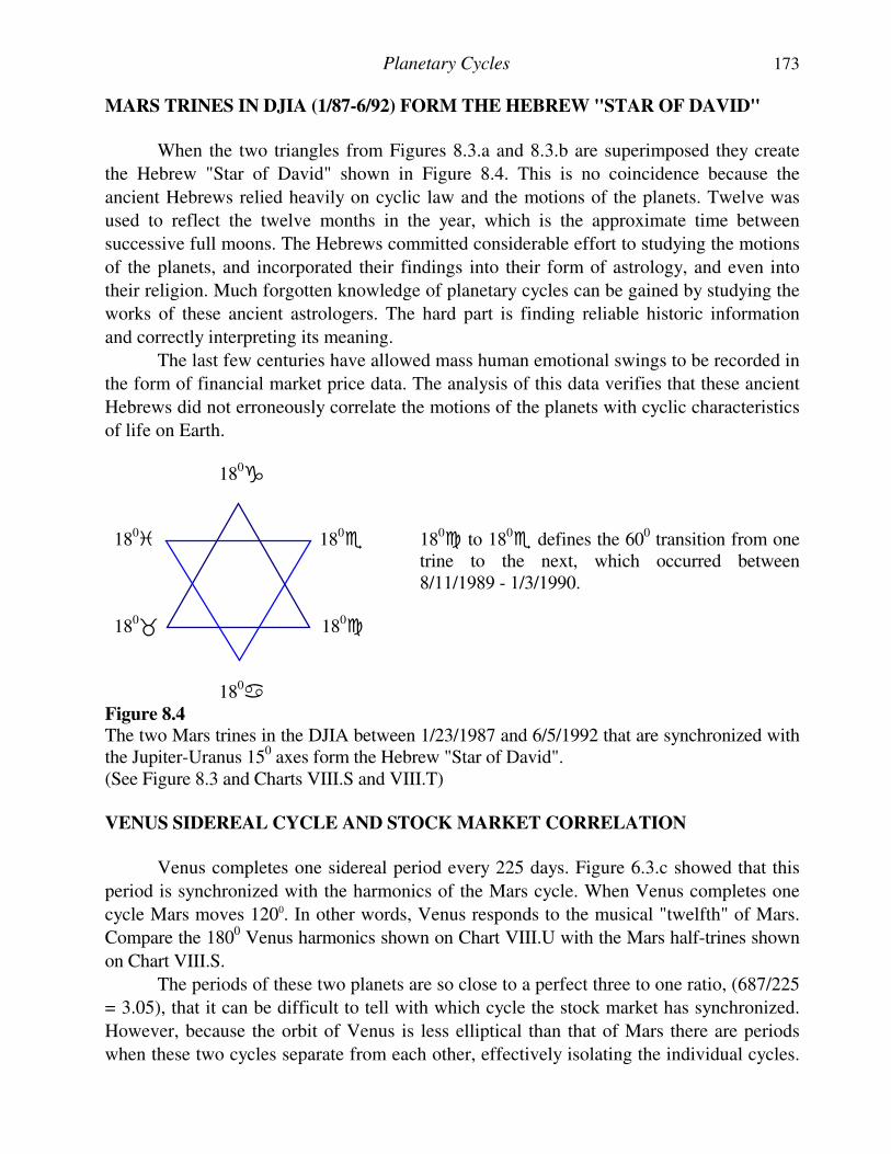
Planetary Cycles 173
MARS TRINES IN DJIA (1/87-6/92) FORM THE HEBREW "STAR OF DAVID"
When the two triangles from Figures 8.3.a and 8.3.b are superimposed they create
the Hebrew "Star of David" shown in Figure 8.4. This is no coincidence because the
ancient Hebrews relied heavily on cyclic law and the motions of the planets. Twelve was
used to reflect the twelve months in the year, which is the approximate time between
successive full moons. The Hebrews committed considerable effort to studying the motions
of the planets, and incorporated their findings into their form of astrology, and even into
their religion. Much forgotten knowledge of planetary cycles can be gained by studying the
works of these ancient astrologers. The hard part is finding reliable historic information
and correctly interpreting its meaning.
The last few centuries have allowed mass human emotional swings to be recorded in
the form of financial market price data. The analysis of this data verifies that these ancient
Hebrews did not erroneously correlate the motions of the planets with cyclic characteristics
of life on Earth. 180 180� 180� 180� to 180� defines the 600 transition from one
trine to the next, which occurred between 8/11/1989 - 1/3/1990.
180� 180� 180� Figure 8.4 The two Mars trines in the DJIA between 1/23/1987 and 6/5/1992 that are synchronized with the Jupiter-Uranus 150 axes form the Hebrew "Star of David". (See Figure 8.3 and Charts VIII.S and VIII.T)
VENUS SIDEREAL CYCLE AND STOCK MARKET CORRELATION
Venus completes one sidereal period every 225 days. Figure 6.3.c showed that this
period is synchronized with the harmonics of the Mars cycle. When Venus completes one
cycle Mars moves 1200. In other words, Venus responds to the musical "twelfth" of Mars.
Compare the 1800 Venus harmonics shown on Chart VIII.U with the Mars half-trines shown
on Chart VIII.S.
The periods of these two planets are so close to a perfect three to one ratio, (687/225
= 3.05), that it can be difficult to tell with which cycle the stock market has synchronized.
However, because the orbit of Venus is less elliptical than that of Mars there are periods
when these two cycles separate from each other, effectively isolating the individual cycles.
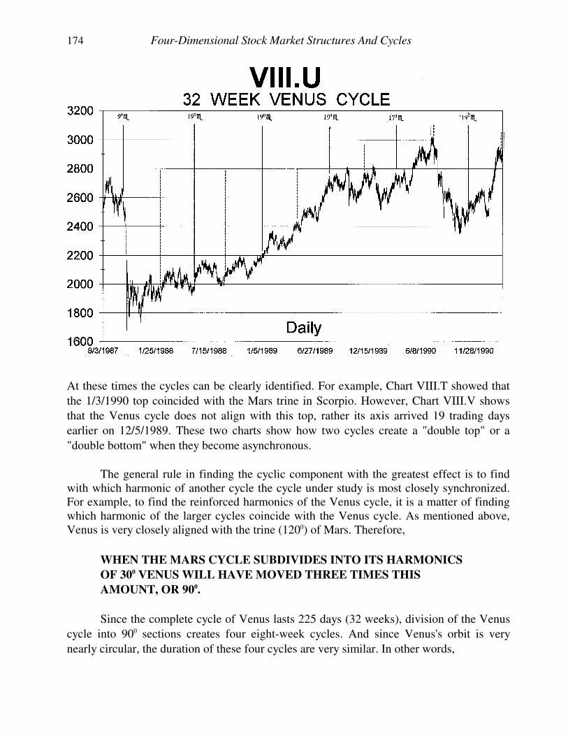
174 Four-Dimensional Stock Market Structures And Cycles
At these times the cycles can be clearly identified. For example, Chart VIII.T showed that
the 1/3/1990 top coincided with the Mars trine in Scorpio. However, Chart VIII.V shows
that the Venus cycle does not align with this top, rather its axis arrived 19 trading days
earlier on 12/5/1989. These two charts show how two cycles create a "double top" or a
"double bottom" when they become asynchronous.
The general rule in finding the cyclic component with the greatest effect is to find with which harmonic of another cycle the cycle under study is most closely synchronized. For example, to find the reinforced harmonics of the Venus cycle, it is a matter of finding which harmonic of the larger cycles coincide with the Venus cycle. As mentioned above, Venus is very closely aligned with the trine (1200) of Mars. Therefore,
WHEN THE MARS CYCLE SUBDIVIDES INTO ITS HARMONICS
OF 300 VENUS WILL HAVE MOVED THREE TIMES THIS
AMOUNT, OR 900.
Since the complete cycle of Venus lasts 225 days (32 weeks), division of the Venus
cycle into 900 sections creates four eight-week cycles. And since Venus's orbit is very
nearly circular, the duration of these four cycles are very similar. In other words,
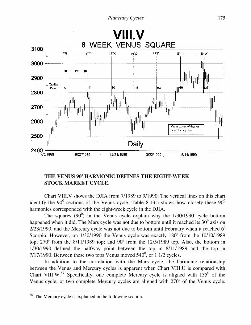
Planetary Cycles 175
THE VENUS 900 HARMONIC DEFINES THE EIGHT-WEEK
STOCK MARKET CYCLE.
Chart VIII.V shows the DJIA from 7/1989 to 9/1990. The vertical lines on this chart
identify the 900 sections of the Venus cycle. Table 8.13.a shows how closely these 900
harmonics corresponded with the eight-week cycle in the DJIA.
The squares (900) in the Venus cycle explain why the 1/30/1990 cycle bottom
happened when it did. The Mars cycle was not due to bottom until it reached its 300 axis on
2/23/1990, and the Mercury cycle was not due to bottom until February when it reached 60
Scorpio. However, on 1/30/1990 the Venus cycle was exactly 1800 from the 10/10/1989
top; 2700 from the 8/11/1989 top; and 900 from the 12/5/1989 top. Also, the bottom in
1/30/1990 defined the halfway point between the top in 8/11/1989 and the top in
7/17/1990. Between these two tops Venus moved 5400, or 1 1/2 cycles.
In addition to the correlation with the Mars cycle, the harmonic relationship
between the Venus and Mercury cycles is apparent when Chart VIII.U is compared with
Chart VIII.W.87 Specifically, one complete Mercury cycle is aligned with 1350 of the
Venus cycle, or two complete Mercury cycles are aligned with 2700 of the Venus cycle.
88 The Mercury cycle is explained in the following section.
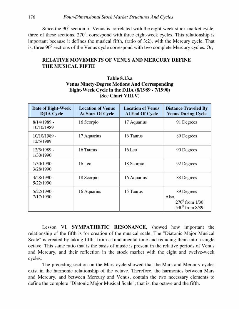
176 Four-Dimensional Stock Market Structures And Cycles
Since the 900 section of Venus is correlated with the eight-week stock market cycle,
three of these sections, 2700, correspond with three eight-week cycles. This relationship is
important because it defines the musical fifth, (ratio of 3:2), with the Mercury cycle. That
is, three 900 sections of the Venus cycle correspond with two complete Mercury cycles. Or,
RELATIVE MOVEMENTS OF VENUS AND MERCURY DEFINE
THE MUSICAL FIFTH
Table 8.13.a
Venus Ninety-Degree Motions And Corresponding
Eight-Week Cycle in the DJIA (8/1989 - 7/1990)
(See Chart VIII.V)
Date of Eight-Week
DJIA Cycle
Location of Venus
At Start Of Cycle
Location of Venus
At End Of Cycle
Distance Traveled By
Venus During Cycle
8/14/1989 - 10/10/1989
16 Scorpio 17 Aquarius 91 Degrees
10/10/1989 - 12/5/1989
17 Aquarius 16 Taurus 89 Degrees
12/5/1989 - 1/30/1990
16 Taurus 16 Leo 90 Degrees
1/30/1990 - 3/28/1990
16 Leo 18 Scorpio 92 Degrees
3/28/1990 - 5/22/1990
18 Scorpio 16 Aquarius 88 Degrees
5/22/1990 - 7/17/1990
16 Aquarius 15 Taurus 89 Degrees Also, 2700 from 1/30 5400 from 8/89
Lesson VI, SYMPATHETIC RESONANCE, showed how important the
relationship of the fifth is for creation of the musical scale. The "Diatonic Major Musical
Scale" is created by taking fifths from a fundamental tone and reducing them into a single
octave. This same ratio that is the basis of music is present in the relative periods of Venus
and Mercury, and their reflection in the stock market with the eight and twelve-week
cycles.
The preceding section on the Mars cycle showed that the Mars and Mercury cycles
exist in the harmonic relationship of the octave. Therefore, the harmonics between Mars
and Mercury, and between Mercury and Venus, contain the two necessary elements to
define the complete "Diatonic Major Musical Scale"; that is, the octave and the fifth.
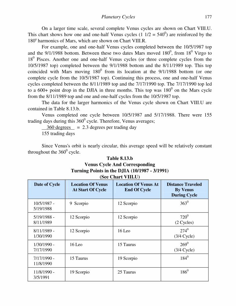
Planetary Cycles 177
On a larger time scale, several complete Venus cycles are shown on Chart VIII.U.
This chart shows how one and one-half Venus cycles (1 1/2 = 5400) are reinforced by the
1800 harmonics of Mars, which are shown on Chart VIII.R.
For example, one and one-half Venus cycles completed between the 10/5/1987 top
and the 9/1/1988 bottom. Between these two dates Mars moved 1800, from 180 Virgo to
180 Pisces. Another one and one-half Venus cycles (or three complete cycles from the
10/5/1987 top) completed between the 9/1/1988 bottom and the 8/11/1989 top. This top
coincided with Mars moving 1800 from its location at the 9/1/1988 bottom (or one
complete cycle from the 10/5/1987 top). Continuing this process, one and one-half Venus
cycles completed between the 8/11/1989 top and the 7/17/1990 top. The 7/17/1990 top led
to a 600+ point drop in the DJIA in three months. This top was 1800 on the Mars cycle
from the 8/11/1989 top and one and one-half cycles from the 10/5/1987 top.
The data for the larger harmonics of the Venus cycle shown on Chart VIII.U are
contained in Table 8.13.b.
Venus completed one cycle between 10/5/1987 and 5/17/1988. There were 155
trading days during this 3600 cycle. Therefore, Venus averages;
360 degrees = 2.3 degrees per trading day
155 trading days
Since Venus's orbit is nearly circular, this average speed will be relatively constant
throughout the 3600 cycle.
Table 8.13.b
Venus Cycle And Corresponding
Turning Points in the DJIA (10/1987 - 3/1991)
(See Chart VIII.U)
Date of Cycle Location Of Venus
At Start Of Cycle
Location Of Venus At
End Of Cycle
Distance Traveled
By Venus
During Cycle
10/5/1987 - 5/19/1988
9 Scorpio 12 Scorpio 3630
5/19/1988 - 8/11/1989
12 Scorpio 12 Scorpio 7200 (2 Cycles)
8/11/1989 - 1/30/1990
12 Scorpio 16 Leo 2740 (3/4 Cycle)
1/30/1990 - 7/17/1990
16 Leo 15 Taurus 2690 (3/4 Cycle)
7/17/1990 - 11/8/1990
15 Taurus 19 Scorpio 1840
11/8/1990 - 3/5/1991
19 Scorpio 25 Taurus 1860
178 Four-Dimensional Stock Market Structures And Cycles
The average of 2.3 degrees that Venus travels per trading day means that when
Venus's location did not align with the ideal cycle by four degrees, as it did at places
shown in Table 8.13.b, this corresponded with less than two trading days. Notice that as the cycles become smaller, the "window of tolerance" is becoming correspondingly narrower. The Venus cycle was shown above to produce results within a two trading day window. This is much narrower than the 7-10 days for the Jupiter-Saturn and Jupiter-Uranus cycles.
12-WEEK MERCURY CYCLE AND STOCK MARKET CORRELATION
Mercury has a sidereal period of 88 days, which is approximately 60 trading days
(twelve weeks). The Mercury cycle is one of the easiest to identify in the stock market
because its period precisely subdivides the periods of the other planets, establishing a close
relationship with their harmonics. This cycle is synchronized with the third octave (450
axes) of the Mars cycle, as shown in Figure 6.3.d.
THE MERCURY CYCLE IS SYNCHRONIZED WITH THE
TWELVE-WEEK STOCK MARKET CYCLE.
Since this cycle only lasts twelve weeks, a daily chart of the DJIA is used to study
its effect. Chart VIII.W identifies the twelve-week cycle with vertical lines and the
corresponding locations of Mercury listed at the tops of these lines.
The data from Chart VIII.W are outlined in Table 8.14 where thirteen twelve-week
cycles are listed with corresponding locations of Mercury. The return of Mercury to 60
Scorpio rarely deviated from these DJIA cycles by more than one or two trading days.
There are several items of special significance in Chart VIII.W. This time period is a
"close-up" view of a section of the Jupiter-Saturn cycles shown on Chart VIII.O. The
section describing the Jupiter-Saturn cycle identified the dates 3/2/1988, 11/16/1988,
8/11/1989, and 4/30/1990 as alternating tops and bottoms in the DJIA (see Table 8.10.b),
correlated with the Jupiter-Saturn cycle. Review these dates on Chart VIII.W and notice
how neatly the Mercury cycle fits into these time intervals. The Jupiter-Saturn cycle topped
out in 3/2/1988 when Mercury was at 60 Scorpio. During this 150 interval of the Jupiter-
Saturn down cycle the market moved sideways. Within this interval Mercury completed
exactly three cycles. Chart VIII.X shows how the interval between 3/2/1988 and
11/16/1988 subdivided into three sections (the musical twelfth).
The Jupiter-Saturn cycle advanced between its 150 axes from 11/16/1988 to
8/11/1989. Within this time interval Mercury again completed exactly three cycles.
Therefore, the complete 300 cycle of Jupiter-Saturn from 3/2/1988 to 8/11/1989 contained
exactly six Mercury cycles.
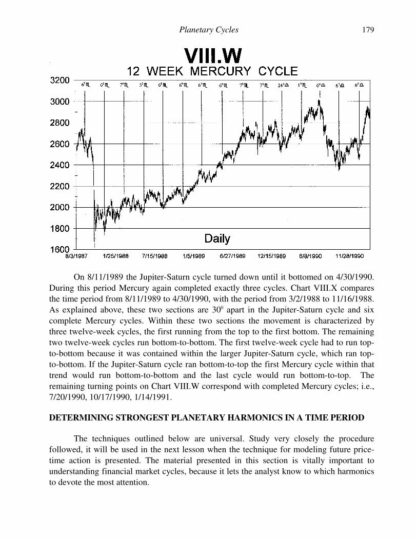
Planetary Cycles 179
On 8/11/1989 the Jupiter-Saturn cycle turned down until it bottomed on 4/30/1990.
During this period Mercury again completed exactly three cycles. Chart VIII.X compares
the time period from 8/11/1989 to 4/30/1990, with the period from 3/2/1988 to 11/16/1988.
As explained above, these two sections are 300 apart in the Jupiter-Saturn cycle and six
complete Mercury cycles. Within these two sections the movement is characterized by
three twelve-week cycles, the first running from the top to the first bottom. The remaining
two twelve-week cycles run bottom-to-bottom. The first twelve-week cycle had to run top-
to-bottom because it was contained within the larger Jupiter-Saturn cycle, which ran top-
to-bottom. If the Jupiter-Saturn cycle ran bottom-to-top the first Mercury cycle within that
trend would run bottom-to-bottom and the last cycle would run bottom-to-top. The
remaining turning points on Chart VIII.W correspond with completed Mercury cycles; i.e.,
7/20/1990, 10/17/1990, 1/14/1991.
DETERMINING STRONGEST PLANETARY HARMONICS IN A TIME PERIOD
The techniques outlined below are universal. Study very closely the procedure
followed, it will be used in the next lesson when the technique for modeling future price-
time action is presented. The material presented in this section is vitally important to
understanding financial market cycles, because it lets the analyst know to which harmonics
to devote the most attention.
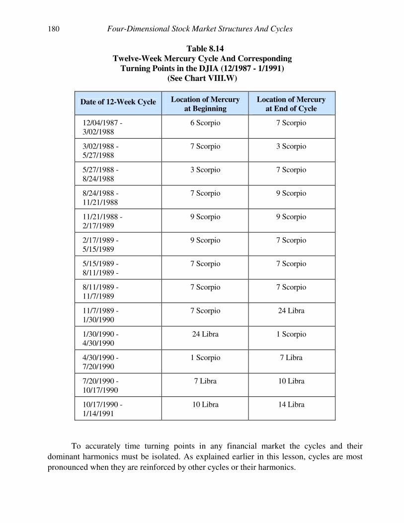
180 Four-Dimensional Stock Market Structures And Cycles
Table 8.14
Twelve-Week Mercury Cycle And Corresponding
Turning Points in the DJIA (12/1987 - 1/1991)
(See Chart VIII.W)
Date of 12-Week Cycle Location of Mercury
at Beginning
Location of Mercury
at End of Cycle
12/04/1987 - 3/02/1988
6 Scorpio 7 Scorpio
3/02/1988 - 5/27/1988
7 Scorpio 3 Scorpio
5/27/1988 - 8/24/1988
3 Scorpio 7 Scorpio
8/24/1988 - 11/21/1988
7 Scorpio 9 Scorpio
11/21/1988 - 2/17/1989
9 Scorpio 9 Scorpio
2/17/1989 - 5/15/1989
9 Scorpio 7 Scorpio
5/15/1989 - 8/11/1989 -
7 Scorpio 7 Scorpio
8/11/1989 - 11/7/1989
7 Scorpio 7 Scorpio
11/7/1989 - 1/30/1990
7 Scorpio 24 Libra
1/30/1990 - 4/30/1990
24 Libra 1 Scorpio
4/30/1990 - 7/20/1990
1 Scorpio 7 Libra
7/20/1990 - 10/17/1990
7 Libra 10 Libra
10/17/1990 - 1/14/1991
10 Libra 14 Libra
To accurately time turning points in any financial market the cycles and their
dominant harmonics must be isolated. As explained earlier in this lesson, cycles are most
pronounced when they are reinforced by other cycles or their harmonics.
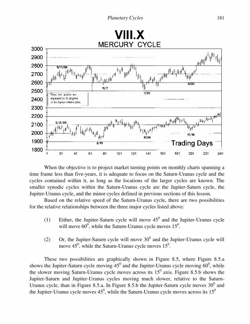
Planetary Cycles 181
When the objective is to project market turning points on monthly charts spanning a
time frame less than five-years, it is adequate to focus on the Saturn-Uranus cycle and the
cycles contained within it, as long as the locations of the larger cycles are known. The
smaller synodic cycles within the Saturn-Uranus cycle are the Jupiter-Saturn cycle, the
Jupiter-Uranus cycle, and the minor cycles defined in previous sections of this lesson.
Based on the relative speed of the Saturn-Uranus cycle, there are two possibilities
for the relative relationships between the three major cycles listed above:
(1) Either, the Jupiter-Saturn cycle will move 450 and the Jupiter-Uranus cycle
will move 600, while the Saturn-Uranus cycle moves 150.
(2) Or, the Jupiter-Saturn cycle will move 300 and the Jupiter-Uranus cycle will
move 450, while the Saturn-Uranus cycle moves 150.
These two possibilities are graphically shown in Figure 8.5, where Figure 8.5.a
shows the Jupiter-Saturn cycle moving 450 and the Jupiter-Uranus cycle moving 600, while
the slower moving Saturn-Uranus cycle moves across its 150 axis. Figure 8.5.b shows the
Jupiter-Saturn and Jupiter-Uranus cycles moving much slower, relative to the Saturn-
Uranus cycle, than in Figure 8.5.a. In Figure 8.5.b the Jupiter-Saturn cycle moves 300 and
the Jupiter-Uranus cycle moves 450, while the Saturn-Uranus cycle moves across its 150
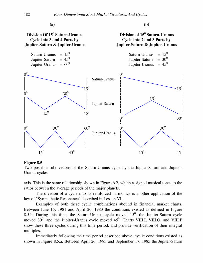
182 Four-Dimensional Stock Market Structures And Cycles
(a) (b)
Division Of 150 Saturn-Uranus Division of 15
0 Saturn-Uranus
Cycle into 3 and 4 Parts by Cycle into 2 and 3 Parts by
Jupiter-Saturn & Jupiter-Uranus Jupiter-Saturn & Jupiter-Uranus Saturn-Uranus = 150 Saturn-Uranus = 150 Jupiter-Saturn = 450 Jupiter-Saturn = 300 Jupiter-Uranus = 600 Jupiter-Uranus = 450 00 00 Saturn-Uranus
150 150 00 300 150 Jupiter-Saturn
150 450 00 300 00 300 600 00 300 Jupiter-Uranus
150 450 150 450
Figure 8.5 Two possible subdivisions of the Saturn-Uranus cycle by the Jupiter-Saturn and Jupiter-Uranus cycles
axis. This is the same relationship shown in Figure 6.2, which assigned musical tones to the
ratios between the average periods of the major planets.
The division of a cycle into its reinforced harmonics is another application of the
law of "Sympathetic Resonance" described in Lesson VI.
Examples of both these cyclic combinations abound in financial market charts.
Between June 15, 1981 and April 26, 1983 the conditions existed as defined in Figure
8.5.b. During this time, the Saturn-Uranus cycle moved 150, the Jupiter-Saturn cycle
moved 300, and the Jupiter-Uranus cycle moved 450. Charts VIII.I, VIII.O, and VIII.P
show these three cycles during this time period, and provide verification of their integral
multiples.
Immediately following the time period described above, cyclic conditions existed as
shown in Figure 8.5.a. Between April 26, 1983 and September 17, 1985 the Jupiter-Saturn
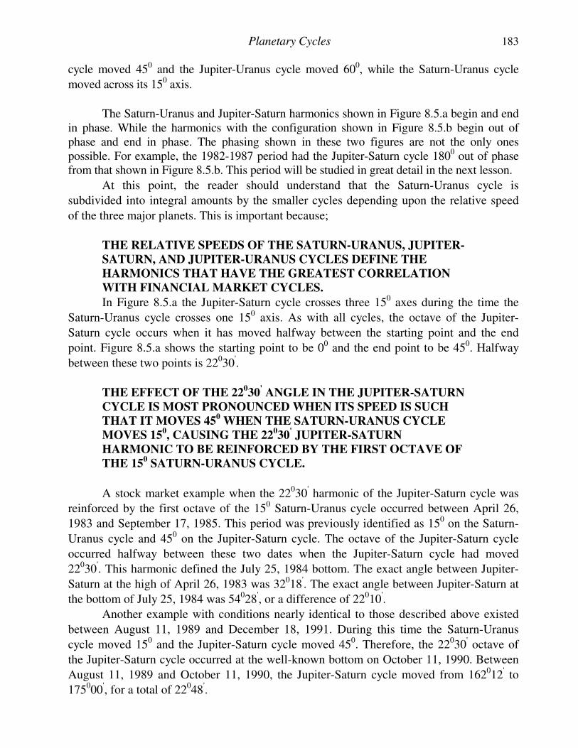
Planetary Cycles 183
cycle moved 450 and the Jupiter-Uranus cycle moved 600, while the Saturn-Uranus cycle
moved across its 150 axis.
The Saturn-Uranus and Jupiter-Saturn harmonics shown in Figure 8.5.a begin and end in phase. While the harmonics with the configuration shown in Figure 8.5.b begin out of phase and end in phase. The phasing shown in these two figures are not the only ones possible. For example, the 1982-1987 period had the Jupiter-Saturn cycle 1800 out of phase from that shown in Figure 8.5.b. This period will be studied in great detail in the next lesson.
At this point, the reader should understand that the Saturn-Uranus cycle is
subdivided into integral amounts by the smaller cycles depending upon the relative speed
of the three major planets. This is important because;
THE RELATIVE SPEEDS OF THE SATURN-URANUS, JUPITER-
SATURN, AND JUPITER-URANUS CYCLES DEFINE THE
HARMONICS THAT HAVE THE GREATEST CORRELATION
WITH FINANCIAL MARKET CYCLES.
In Figure 8.5.a the Jupiter-Saturn cycle crosses three 150 axes during the time the
Saturn-Uranus cycle crosses one 150 axis. As with all cycles, the octave of the Jupiter-
Saturn cycle occurs when it has moved halfway between the starting point and the end
point. Figure 8.5.a shows the starting point to be 00 and the end point to be 450. Halfway
between these two points is 22030'.
THE EFFECT OF THE 22030
' ANGLE IN THE JUPITER-SATURN
CYCLE IS MOST PRONOUNCED WHEN ITS SPEED IS SUCH
THAT IT MOVES 450 WHEN THE SATURN-URANUS CYCLE
MOVES 150, CAUSING THE 22
030
' JUPITER-SATURN
HARMONIC TO BE REINFORCED BY THE FIRST OCTAVE OF
THE 150 SATURN-URANUS CYCLE.
A stock market example when the 22030' harmonic of the Jupiter-Saturn cycle was
reinforced by the first octave of the 150 Saturn-Uranus cycle occurred between April 26,
1983 and September 17, 1985. This period was previously identified as 150 on the Saturn-
Uranus cycle and 450 on the Jupiter-Saturn cycle. The octave of the Jupiter-Saturn cycle
occurred halfway between these two dates when the Jupiter-Saturn cycle had moved
22030'. This harmonic defined the July 25, 1984 bottom. The exact angle between Jupiter-
Saturn at the high of April 26, 1983 was 32018'. The exact angle between Jupiter-Saturn at
the bottom of July 25, 1984 was 54028', or a difference of 22010'.
Another example with conditions nearly identical to those described above existed
between August 11, 1989 and December 18, 1991. During this time the Saturn-Uranus
cycle moved 150 and the Jupiter-Saturn cycle moved 450. Therefore, the 22030' octave of
the Jupiter-Saturn cycle occurred at the well-known bottom on October 11, 1990. Between
August 11, 1989 and October 11, 1990, the Jupiter-Saturn cycle moved from 162012' to
175000', for a total of 22048'.
184 Four-Dimensional Stock Market Structures And Cycles
Similarly, the top just before the crash on October 5,1987 occurred when the
Jupiter-Saturn cycle reached 122000'. This was 22048' from the bottom on September 29,
1986 and 44050' from the bottom on September 17, 1985. Therefore, the bottom on
September 29, 1986 coincided with the octave of the 450 Jupiter-Saturn cycle, measured
between September 17, 1985 and October 5, 1987.
The deviations from the ideal 22030' octave and the date of the actual turning points
rarely lasted more than one or two trading days. Remember, the Jupiter-Saturn cycle is one
of the larger cycles. To narrow the exact date of the turning point smaller cycles are used.
The examples given above of the 22030' harmonic occurred within time frames
when the cyclic combinations were as shown in Figure 8.5.a. The effect of this harmonic is
greatly attenuated when the Jupiter-Saturn cycle moves 300 within the Saturn-Uranus 150
cycle, as shown in Figure 8.5.b. The reason for this becomes clear if Figure 8.5.b is
studied. When the Jupiter-Saturn cycle moves 22030', with the type of arrangement shown
in Figure 8.5.b, it will not coincide with the first octave of the Saturn-Uranus 150 cycle.
Rather, the Saturn-Uranus cycle will have moved through three-quarters of its cycle,
corresponding with the second octave. The magnitude of the second octave is less than the
first octave. Similarly, this 22030' harmonic of the Jupiter-Saturn cycle is not reinforced by
a major harmonic of the Jupiter-Uranus cycle, this cycle moving approximately 340 during
this time.
An example of the cyclic combination shown in Figure 8.5.b occurred between June
15, 1981 and April 26, 1983. During this time the Jupiter-Saturn cycle moved 300 within
the larger Saturn-Uranus 150 cycle. The 22030' harmonic is measured from the node
defining the beginning of this cycle on June 15, 1981. This 22030' harmonic arrived in
November, 1982 and had minimal effect on the stock market, as can be seen on Chart
VIII.O. The Jupiter-Saturn octave during this period was not the 22030' division, rather it
occurred at 150. This harmonic corresponded with the major bottom in March, 1982.
To make this concept clearer, Figure 8.6 shows how the dominant harmonic changes
from 150 to 22030' during a theoretical period of time. Figure 8.6.a shows the larger Saturn-
Uranus cycle moving across three 150 axes. In Figure 8.6.b the Jupiter-Saturn cycle moves
300 during the first Saturn-Uranus 150 cycle, and 450 during the second and third Saturn-
Uranus 150 cycles. Figure 8.6.c shows the octave of the Jupiter-Saturn cycle shown in
Figure 8.6.b. The duration of the first two half-cycles in Figure 8.6.c is 150 of the Jupiter-
Saturn cycle. However, the remaining half-cycles in Figure 8.6.c have 22030' durations. All
the cycles in Figure 8.6.c are the result of subdividing the Jupiter-Saturn cycle shown in
Figure 8.6.b into two parts, but the values change from 150 to 22030' because the larger
Jupiter-Saturn cycle changes from 300 to 450.
This theoretical example actually happened between the dates of June 15, 1981 and
October 5, 1987, as shown on Charts VIII.I and VIII.O.
The conclusion to be drawn from the above discussion is that measuring 22030' from
a node on the Jupiter-Saturn cycle identifies a significant turning point in the stock market
only if the relative speed of the cycles are as shown in Figure 8.5.b. That is, the Jupiter-
Saturn cycle must move through 450 during a 150 motion of the larger Saturn-Uranus cycle.
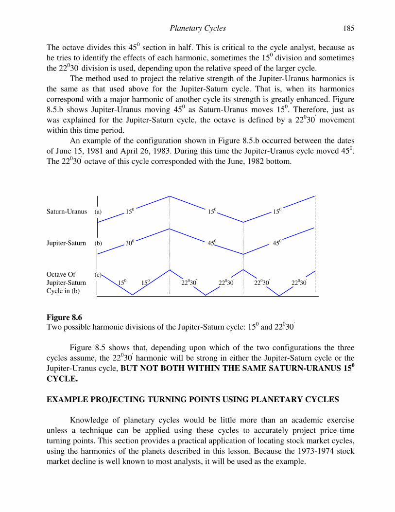
Planetary Cycles 185
The octave divides this 450 section in half. This is critical to the cycle analyst, because as
he tries to identify the effects of each harmonic, sometimes the 150 division and sometimes
the 22030' division is used, depending upon the relative speed of the larger cycle.
The method used to project the relative strength of the Jupiter-Uranus harmonics is
the same as that used above for the Jupiter-Saturn cycle. That is, when its harmonics
correspond with a major harmonic of another cycle its strength is greatly enhanced. Figure
8.5.b shows Jupiter-Uranus moving 450 as Saturn-Uranus moves 150. Therefore, just as
was explained for the Jupiter-Saturn cycle, the octave is defined by a 22030' movement
within this time period.
An example of the configuration shown in Figure 8.5.b occurred between the dates
of June 15, 1981 and April 26, 1983. During this time the Jupiter-Uranus cycle moved 450.
The 22030' octave of this cycle corresponded with the June, 1982 bottom.
Saturn-Uranus (a) 150 150 150
Jupiter-Saturn (b) 300 450 450
Octave Of (c)
Jupiter-Saturn 150 150 22030' 22030' 22030' 22030'
Cycle in (b)
Figure 8.6 Two possible harmonic divisions of the Jupiter-Saturn cycle: 150 and 22030'
Figure 8.5 shows that, depending upon which of the two configurations the three
cycles assume, the 22030' harmonic will be strong in either the Jupiter-Saturn cycle or the
Jupiter-Uranus cycle, BUT NOT BOTH WITHIN THE SAME SATURN-URANUS 150
CYCLE.
EXAMPLE PROJECTING TURNING POINTS USING PLANETARY CYCLES
Knowledge of planetary cycles would be little more than an academic exercise
unless a technique can be applied using these cycles to accurately project price-time
turning points. This section provides a practical application of locating stock market cycles,
using the harmonics of the planets described in this lesson. Because the 1973-1974 stock
market decline is well known to most analysts, it will be used as the example.
186 Four-Dimensional Stock Market Structures And Cycles
January, 1973 would have easily been identified in advance as a turning point in the
stock market for a variety of reasons. Just a few of these reasons are:
(1) Uranus seven-year cycle was 300 from the beginning of the square in 2/1966,
and due to bottom when it reached its 00 axis in two years.
(2) Uranus cycle was 1800 from the low in 7/1932.
(3) Saturn-Uranus cycle was 600 from the beginning of the square in 2/1966.
(4) Saturn-Uranus cycle was 300 from the top in 5/1969.
(5) Saturn-Uranus cycle was completing a 3600 cycle from the top in 9/1929.
(6) Saturn cycle was 900 from the beginning of the square in 2/1966.
(7) Saturn was in Gemini; as it was in 1942, 1914, 1884, etc.
(8) Jupiter-Uranus cycle was 900 from the top in 5/1969, and 600 from the
bottom in 7/1970.
(9) Jupiter-Saturn cycle was 600 from the top in 12/1968.
(10) Mars returned to 190 Scorpio, which was its location at the tops in 4/1971
and 4/1969.
For the reasons outlined above, the analyst would have concluded that January,
1973 represented a cyclic turning point in the stock market. If it is not clear how this
conclusion was reached, reread the sections in this lesson describing these cycles.
Even if the date of this top had not been identified in advance, within two weeks it
would have been clear that a major decline was under way, since prices declined nearly ten
percent during the first two weeks.
Since prices had been increasing into the January, 1973 turning point, the task
became one of determining how long the ensuing decline would last and when intervening
countertrend rallies would occur within this decline.
As explained in the section on the Uranus cycle, the twenty-one year Uranus
quarter-cycle and seven year Uranus cycle were pointing down during this time. Therefore,
the objective focuses on projecting what will happen for the two or three years between the
nodal point in January, 1973 and the expected seven year Uranus cycle bottom in early
1975. The largest cycle corresponding with this time frame occurs along the 150 axes of the
Saturn-Uranus cycle, which averages 22.5 months per 150 axis.
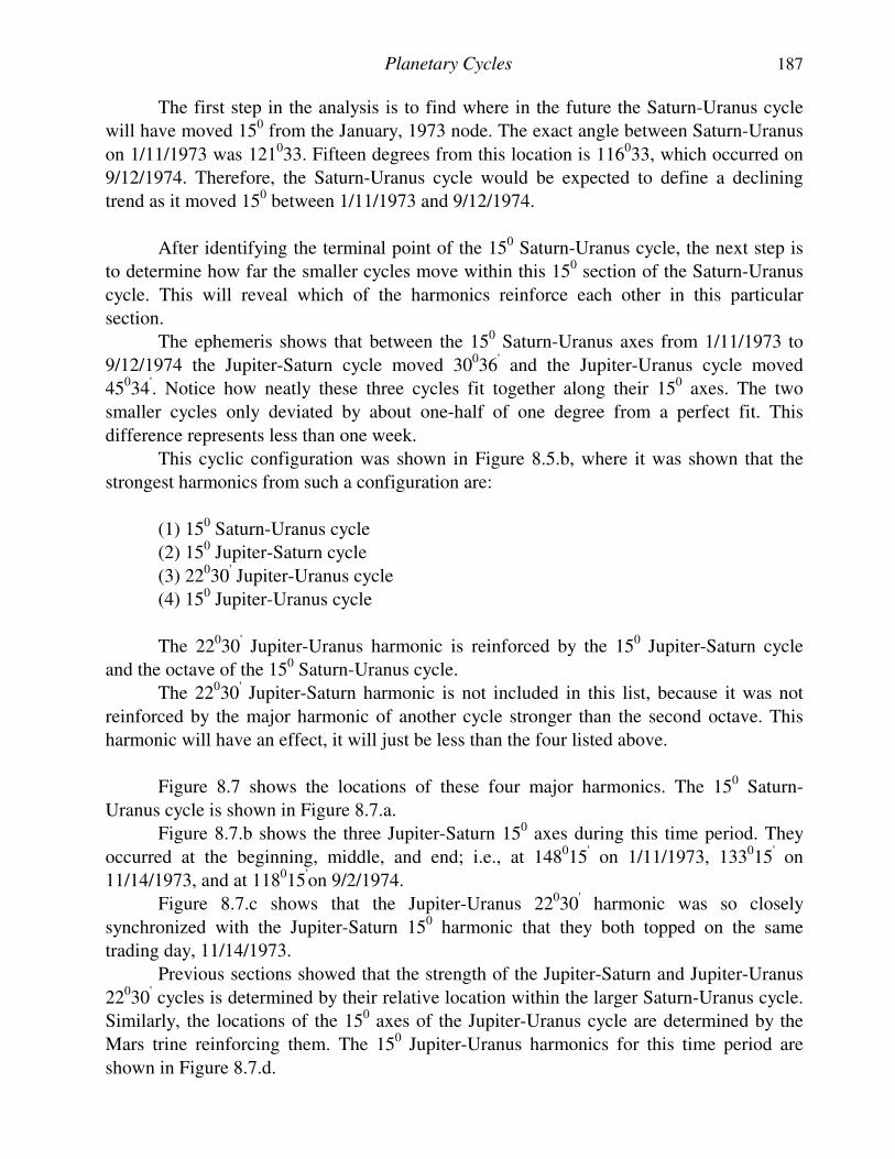
Planetary Cycles 187
The first step in the analysis is to find where in the future the Saturn-Uranus cycle
will have moved 150 from the January, 1973 node. The exact angle between Saturn-Uranus
on 1/11/1973 was 121033. Fifteen degrees from this location is 116033, which occurred on
9/12/1974. Therefore, the Saturn-Uranus cycle would be expected to define a declining
trend as it moved 150 between 1/11/1973 and 9/12/1974.
After identifying the terminal point of the 150 Saturn-Uranus cycle, the next step is
to determine how far the smaller cycles move within this 150 section of the Saturn-Uranus
cycle. This will reveal which of the harmonics reinforce each other in this particular
section.
The ephemeris shows that between the 150 Saturn-Uranus axes from 1/11/1973 to
9/12/1974 the Jupiter-Saturn cycle moved 30036' and the Jupiter-Uranus cycle moved
45034'. Notice how neatly these three cycles fit together along their 150 axes. The two
smaller cycles only deviated by about one-half of one degree from a perfect fit. This
difference represents less than one week.
This cyclic configuration was shown in Figure 8.5.b, where it was shown that the
strongest harmonics from such a configuration are:
(1) 150 Saturn-Uranus cycle
(2) 150 Jupiter-Saturn cycle
(3) 22030' Jupiter-Uranus cycle
(4) 150 Jupiter-Uranus cycle
The 22030' Jupiter-Uranus harmonic is reinforced by the 150 Jupiter-Saturn cycle
and the octave of the 150 Saturn-Uranus cycle.
The 22030' Jupiter-Saturn harmonic is not included in this list, because it was not
reinforced by the major harmonic of another cycle stronger than the second octave. This
harmonic will have an effect, it will just be less than the four listed above.
Figure 8.7 shows the locations of these four major harmonics. The 150 Saturn-
Uranus cycle is shown in Figure 8.7.a.
Figure 8.7.b shows the three Jupiter-Saturn 150 axes during this time period. They
occurred at the beginning, middle, and end; i.e., at 148015' on 1/11/1973, 133015' on
11/14/1973, and at 118015'on 9/2/1974.
Figure 8.7.c shows that the Jupiter-Uranus 22030' harmonic was so closely
synchronized with the Jupiter-Saturn 150 harmonic that they both topped on the same
trading day, 11/14/1973.
Previous sections showed that the strength of the Jupiter-Saturn and Jupiter-Uranus
22030' cycles is determined by their relative location within the larger Saturn-Uranus cycle.
Similarly, the locations of the 150 axes of the Jupiter-Uranus cycle are determined by the
Mars trine reinforcing them. The 150 Jupiter-Uranus harmonics for this time period are
shown in Figure 8.7.d.
188 Four-Dimensional Stock Market Structures And Cycles
There is a very critical characteristic of this harmonic of which the analyst must be
aware. The starting date of the Jupiter-Uranus 150 axis is 1/25/1973. This date was
determined by the synchrony that exists between this harmonic and the Mars trine.
However, the starting date for the Jupiter-Uranus 22030' harmonic is determined by its
synchrony with the larger Saturn-Uranus and Jupiter-Saturn harmonics. EVEN THOUGH THE RELATIVE MOTION OF THE SAME TWO
PLANETS (JUPITER AND URANUS) DEFINES THE 150 AND 22
030
'
HARMONICS, THE PRECISE LOCATIONS OF THESE TWO
HARMONICS ARE DETERMINED BY THEIR SYNCHRONY WITH
THE HARMONICS OF DIFFERENT PLANETS. THE 150 HARMONIC
IS SYNCHRONIZED WITH THE MARS TRINE AND THE 22030
'
HARMONIC IS SYNCHRONIZED WITH THE SATURN-URANUS
AND JUPITER-SATURN CYCLES.
The active Mars trine for this period is shown in Figure 8.7.e. This is the same trine
shown in Figure 8.3.b. The first three axes of this trine were closely synchronized with the
Jupiter-Uranus 150 axes shown in Figure 8.7.d. These two harmonics became asynchronous
when Mars slowed down as it approached aphelion in Virgo. At this point the Jupiter-
Uranus 150 harmonic became synchronized with the new Mars trine shown in Figure 8.3.a.
This "decoupling" from the first Mars trine can be seen in Figures 8.7.d and 8.7.e where the
Jupiter-Uranus cycle bottomed on 9/20/1974 and the Mars trine bottomed three months
later on 12/12/1974.
Chart VIII.Y shows the cycles from Figure 8.7 overlaid on the DJIA. The Jupiter-
Saturn 150 harmonic and the Jupiter-Uranus 22030' harmonic were so closely synchronized
that they are shown as the same cycle on this Chart. The axes of these two combined
harmonics coincided with the dramatic decline in November, 1973.
The 150 Jupiter-Uranus harmonic and its associated Mars trine turned up between August, 1973 and March, 1974. These cycles coincided with the countertrend rally during this time. The two bottoms in October, 1974 and December, 1974 coincided with the Jupiter-Uranus 150 harmonic and the Mars trine becoming asynchronous at that time, as shown in Figures 8.7.d and 8.7.e. This was an example of the double bottom formation caused by cycles not arriving at their axes simultaneously.
SUMMARY
This lesson analyzed the correlation between each of the planetary cycles and
stock market cycles. Briefly summarized, the topics included:
A. Stock market cycles resonate sympathetically with the heliocentric motions
of the planets.
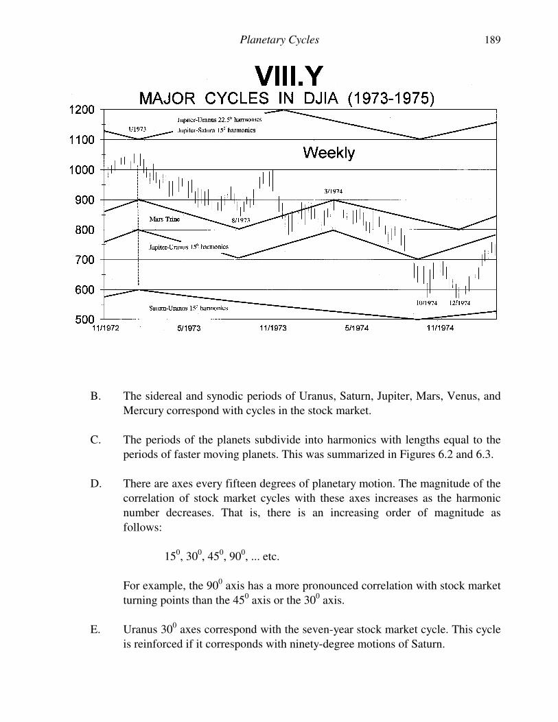
Planetary Cycles 189
B. The sidereal and synodic periods of Uranus, Saturn, Jupiter, Mars, Venus, and
Mercury correspond with cycles in the stock market.
C. The periods of the planets subdivide into harmonics with lengths equal to the
periods of faster moving planets. This was summarized in Figures 6.2 and 6.3.
D. There are axes every fifteen degrees of planetary motion. The magnitude of the
correlation of stock market cycles with these axes increases as the harmonic
number decreases. That is, there is an increasing order of magnitude as
follows:
150, 300, 450, 900, ... etc.
For example, the 900 axis has a more pronounced correlation with stock market
turning points than the 450 axis or the 300 axis.
E. Uranus 300 axes correspond with the seven-year stock market cycle. This cycle
is reinforced if it corresponds with ninety-degree motions of Saturn.
190 Four-Dimensional Stock Market Structures And Cycles
F. The Uranus quarter-cycle averages twenty-one years and corresponds with an
alternating trend of stock market prices.
G. Saturn 600 axes correspond with the five-year stock market cycle.
H. Saturn has two significant nodal areas located 1800 apart in Gemini and
Sagittarius. These nodes are in the same signs as the Uranus nodes.
I. The Saturn-Uranus synodic cycle of forty-five-years has axes every 150,
averaging 22.5 months, that correspond with changing trends in the stock
market.
J. The Saturn-Uranus synodic cycle defined the 52-month stock market cycle
during the 1949-1966 and 1982-1987 squares.
K. The Saturn-Uranus synodic cycle defined the 42-month stock market cycle
during the 1966-1982 square.
L. One and one-half Saturn-Uranus synodic cycles corresponded with the 67-year
interval between similar faces of the two major cubes defined in Lesson V.
M. The Jupiter-Uranus synodic cycle of fourteen years has axes every 150,
averaging 7 months, that correspond with changing trends in the stock market.
N. The Jupiter-Saturn synodic cycle of twenty years has axes every 150, averaging
10 months, that correspond with changing trends in the stock market.
O. The 22030' harmonic is most pronounced in either the Jupiter-Saturn cycle or
the Jupiter-Uranus cycle, depending upon which of these two cycles moves 450
within the larger Saturn-Uranus 150 harmonic.
P. The Mars trine corresponds with the 150 Jupiter-Uranus harmonic, and shifts to
a new trine when these two cycles become asynchronous. This typically
happens when Mars is at the slowest point in its orbit, in Virgo.
Q. The Mars square (900) corresponds with two Mercury cycles and two twelve-
week stock market cycles.
R. The Venus square (900) corresponds with the eight0week stock market cycle.
S. The Mercury cycle corresponds with the twelve0week stock market cycle.
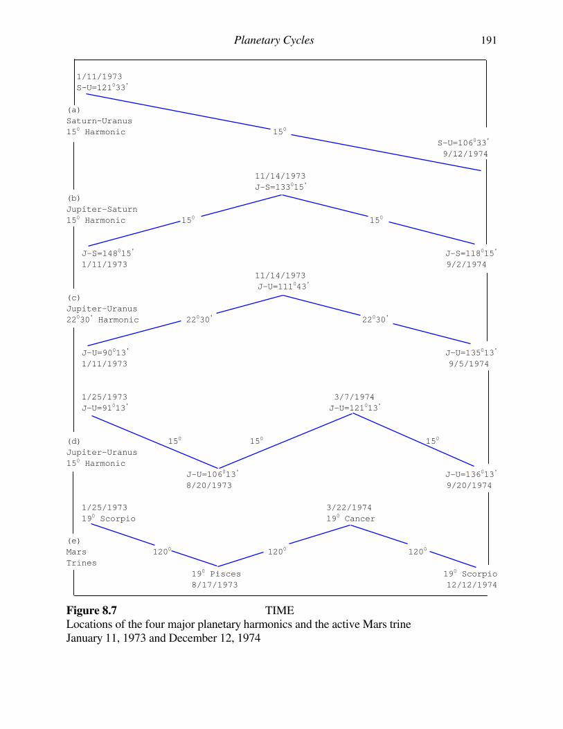
Planetary Cycles 191
1/11/1973
S-U=121033'
(a)
Saturn-Uranus
150 Harmonic 150
S-U=106033'
9/12/1974
11/14/1973
J-S=133015'
(b)
Jupiter-Saturn
150 Harmonic 150 150
J-S=148015' J-S=118015'
1/11/1973 9/2/1974
11/14/1973
J-U=111043'
(c)
Jupiter-Uranus
22030' Harmonic 22030' 22030'
J-U=90013' J-U=135013'
1/11/1973 9/5/1974
1/25/1973 3/7/1974
J-U=91013' J-U=121013'
(d) 150 150 150
Jupiter-Uranus
150 Harmonic
J-U=106013' J-U=136013'
8/20/1973 9/20/1974
1/25/1973 3/22/1974
190 Scorpio 190 Cancer
(e)
Mars 1200 1200 1200
Trines
190 Pisces 190 Scorpio
8/17/1973 12/12/1974
Figure 8.7 TIME
Locations of the four major planetary harmonics and the active Mars trine January 11, 1973 and December 12, 1974
LESSON IX
COMPOSITE CYCLES:
PUTTING IT ALL TOGETHER It is sufficiently agreed that all things change, and that nothing really disappears, but that the sum of matter remains
exactly the same.
Francis Bacon (1626 A.D.) ...Cogitationes de Natura Rerum
INTRODUCTION
Previous lessons studied the correlation between cycles in the stock market and
motions of the planets across their 150 axes. Each of these cycles and their harmonics
exert their own influence on mass human psychology, which can be identified and
measured by studying relative price-time changes. The net effect of these individual
cycles, known as simple components, is called the "composite wave", and is what is seen
on price-time charts.
This lesson will use the planetary cycles and their harmonics, identified in Lesson
VIII, PLANETARY CYCLES, as simple components to create a composite wave that
accurately models stock market price-time behavior. The techniques employed are unique
in the fact that they are based upon a determination of dominant planetary harmonics and
the boundaries containing these effects based upon the geometry from Part I. Regardless
of the time period studied, past or future, the techniques used below to create the
composite wave can be used to model price-time. The principles are equally applicable to
any time period because the motions of the planets and their corresponding harmonics are
not only easily calculated years in the past, but also into the future.
To develop a composite wave from individual simple cycles the technique
described in Lesson VII, CYCLES, which removed the individual components from
existing stock market data, is reversed. This approach differs from those used by
contemporary cycle analysts who try to create an accurate composite model by adding
together a variety of simple components and expect this SUM to model financial market
behavior. However, as was demonstrated in Lesson VII, CYCLES, this sum only creates
the PERCENT DEVIATION FROM THE TREND. To arrive at the final model, THE
SUM MUST BE MULTIPLIED BY THE LARGER TREND.
CONTEMPORARY METHODS FOR CREATING COMPOSITE WAVES
Market analysts have tried for years to create a composite wave that reliably
predicts financial market behavior. The most commonly used approach is the simple
"sum of sin waves", which uses sin waves as simple components. These "cycles", which
are actually rhythms, are shown in Figure 9.1.
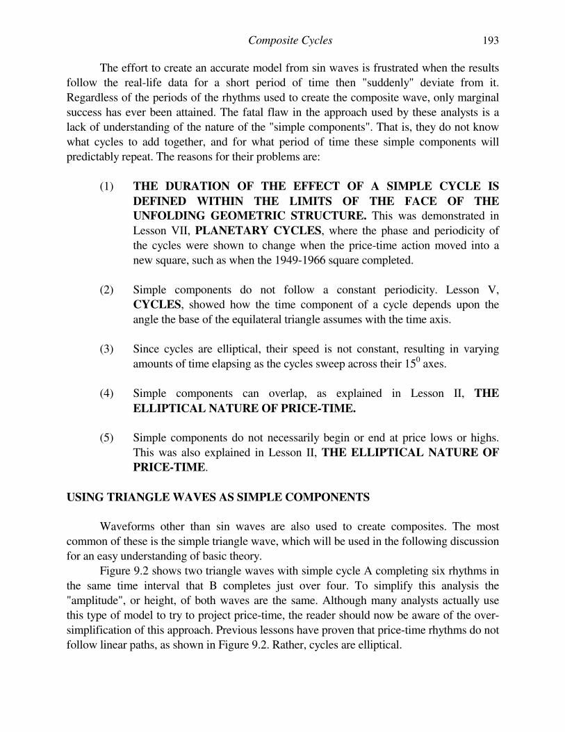
Composite Cycles 193
The effort to create an accurate model from sin waves is frustrated when the results
follow the real-life data for a short period of time then "suddenly" deviate from it.
Regardless of the periods of the rhythms used to create the composite wave, only marginal
success has ever been attained. The fatal flaw in the approach used by these analysts is a
lack of understanding of the nature of the "simple components". That is, they do not know
what cycles to add together, and for what period of time these simple components will
predictably repeat. The reasons for their problems are:
(1) THE DURATION OF THE EFFECT OF A SIMPLE CYCLE IS
DEFINED WITHIN THE LIMITS OF THE FACE OF THE
UNFOLDING GEOMETRIC STRUCTURE. This was demonstrated in
Lesson VII, PLANETARY CYCLES, where the phase and periodicity of
the cycles were shown to change when the price-time action moved into a
new square, such as when the 1949-1966 square completed.
(2) Simple components do not follow a constant periodicity. Lesson V,
CYCLES, showed how the time component of a cycle depends upon the
angle the base of the equilateral triangle assumes with the time axis.
(3) Since cycles are elliptical, their speed is not constant, resulting in varying
amounts of time elapsing as the cycles sweep across their 150 axes.
(4) Simple components can overlap, as explained in Lesson II, THE
ELLIPTICAL NATURE OF PRICE-TIME.
(5) Simple components do not necessarily begin or end at price lows or highs.
This was also explained in Lesson II, THE ELLIPTICAL NATURE OF
PRICE-TIME.
USING TRIANGLE WAVES AS SIMPLE COMPONENTS
Waveforms other than sin waves are also used to create composites. The most
common of these is the simple triangle wave, which will be used in the following discussion
for an easy understanding of basic theory.
Figure 9.2 shows two triangle waves with simple cycle A completing six rhythms in
the same time interval that B completes just over four. To simplify this analysis the
"amplitude", or height, of both waves are the same. Although many analysts actually use
this type of model to try to project price-time, the reader should now be aware of the over-
simplification of this approach. Previous lessons have proven that price-time rhythms do not
follow linear paths, as shown in Figure 9.2. Rather, cycles are elliptical.
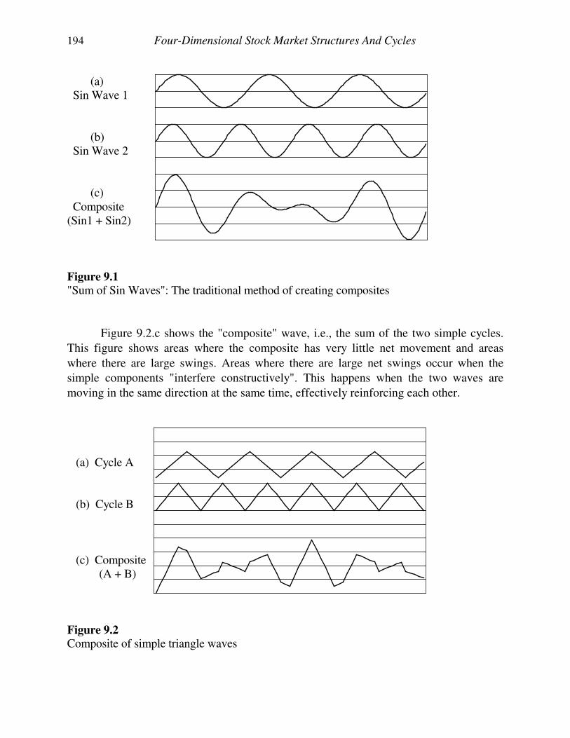
194 Four-Dimensional Stock Market Structures And Cycles
(a) Sin Wave 1 (b) Sin Wave 2 (c) Composite (Sin1 + Sin2)
Figure 9.1 "Sum of Sin Waves": The traditional method of creating composites
Figure 9.2.c shows the "composite" wave, i.e., the sum of the two simple cycles.
This figure shows areas where the composite has very little net movement and areas
where there are large swings. Areas where there are large net swings occur when the
simple components "interfere constructively". This happens when the two waves are
moving in the same direction at the same time, effectively reinforcing each other. (a) Cycle A (b) Cycle B (c) Composite (A + B)
Figure 9.2 Composite of simple triangle waves
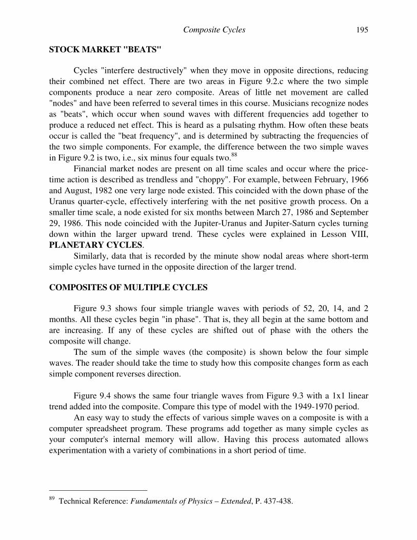
Composite Cycles 195
STOCK MARKET "BEATS"
Cycles "interfere destructively" when they move in opposite directions, reducing
their combined net effect. There are two areas in Figure 9.2.c where the two simple
components produce a near zero composite. Areas of little net movement are called
"nodes" and have been referred to several times in this course. Musicians recognize nodes
as "beats", which occur when sound waves with different frequencies add together to
produce a reduced net effect. This is heard as a pulsating rhythm. How often these beats
occur is called the "beat frequency", and is determined by subtracting the frequencies of
the two simple components. For example, the difference between the two simple waves
in Figure 9.2 is two, i.e., six minus four equals two.88
Financial market nodes are present on all time scales and occur where the price-
time action is described as trendless and "choppy". For example, between February, 1966
and August, 1982 one very large node existed. This coincided with the down phase of the
Uranus quarter-cycle, effectively interfering with the net positive growth process. On a
smaller time scale, a node existed for six months between March 27, 1986 and September
29, 1986. This node coincided with the Jupiter-Uranus and Jupiter-Saturn cycles turning
down within the larger upward trend. These cycles were explained in Lesson VIII,
PLANETARY CYCLES.
Similarly, data that is recorded by the minute show nodal areas where short-term
simple cycles have turned in the opposite direction of the larger trend.
COMPOSITES OF MULTIPLE CYCLES
Figure 9.3 shows four simple triangle waves with periods of 52, 20, 14, and 2
months. All these cycles begin "in phase". That is, they all begin at the same bottom and
are increasing. If any of these cycles are shifted out of phase with the others the
composite will change.
The sum of the simple waves (the composite) is shown below the four simple
waves. The reader should take the time to study how this composite changes form as each
simple component reverses direction.
Figure 9.4 shows the same four triangle waves from Figure 9.3 with a 1x1 linear
trend added into the composite. Compare this type of model with the 1949-1970 period.
An easy way to study the effects of various simple waves on a composite is with a
computer spreadsheet program. These programs add together as many simple cycles as
your computer's internal memory will allow. Having this process automated allows
experimentation with a variety of combinations in a short period of time.
89 Technical Reference: Fundamentals of Physics – Extended, P. 437-438.
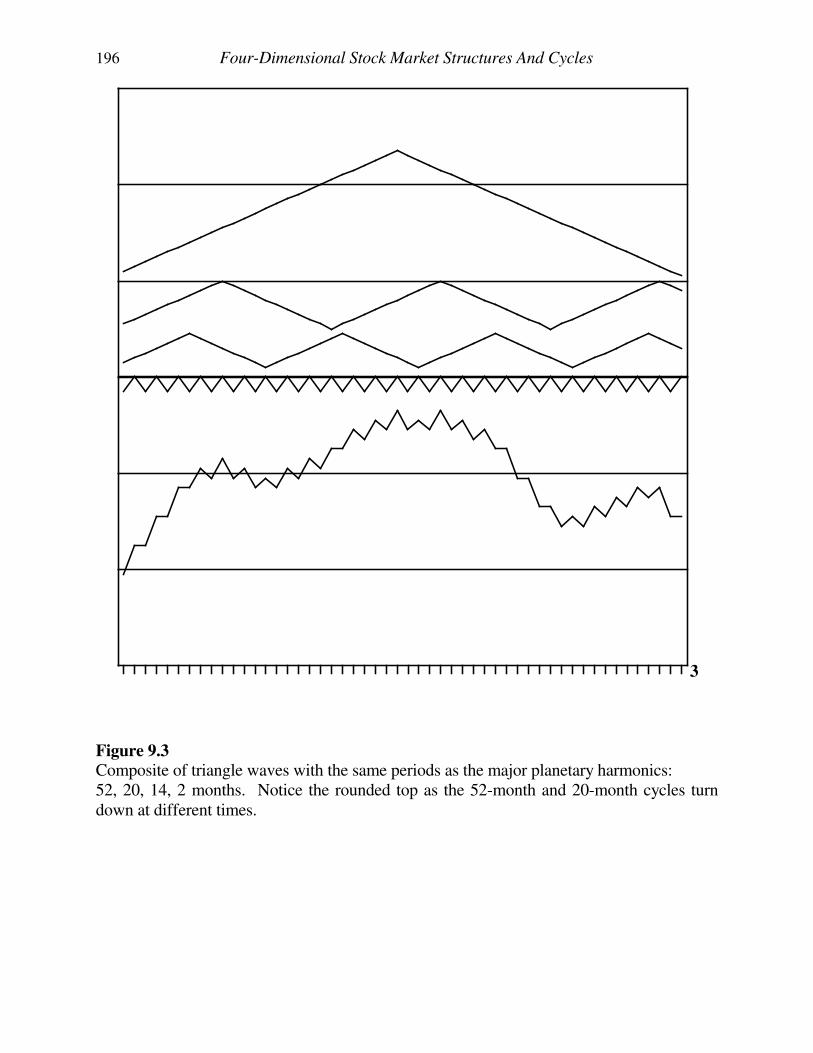
196 Four-Dimensional Stock Market Structures And Cycles
3
Figure 9.3 Composite of triangle waves with the same periods as the major planetary harmonics: 52, 20, 14, 2 months. Notice the rounded top as the 52-month and 20-month cycles turn down at different times.
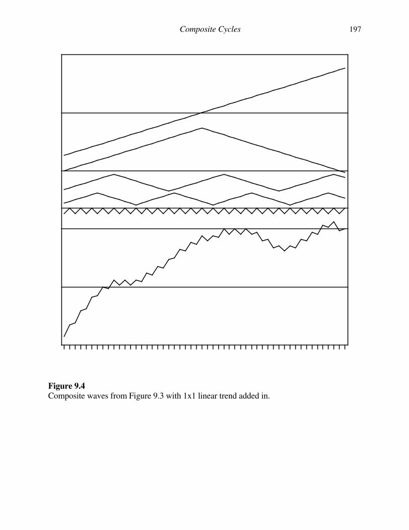
Composite Cycles 197
Figure 9.4 Composite waves from Figure 9.3 with 1x1 linear trend added in.
198 Four-Dimensional Stock Market Structures And Cycles
CREATING THE REAL-LIFE COMPOSITE OF THE STOCK MARKET
Lesson V, CYCLES, showed how cycles are traditionally isolated in financial
markets by analysis of the percent deviation from a moving average. This approach starts
with a composite wave, removes the trend by dividing the price-time data into the
moving average, then subtracts out each individual cyclic component, i.e., the simple
cycles.
To produce a composite wave the methods used in Lesson V are reversed. That is,
(1) The individual cyclic components are added together producing the percent
deviation from the underlying trend.
(2) The future trend is determined by analysis of the locations of the longest
cycles. This trend is a function of the length of the time frame being studied. If
a seven-year trend is large enough the motion of Uranus between its 300 axes
is used. If a trend longer than seven years is needed the 21-year Uranus
quarter-cycle is used, and the seven-year cycle becomes another simple
component to be added into the composite.
The Saturn five-year cycle is used for the trend if the analysis covers five-
years or less the.
(3) The result of the addition of the simple components in step (1) is multiplied by
the trend from step (2).
To demonstrate how closely this method predicts stock market activity, the well-
known period from the low on August 11, 1982 until the crash in October, 1987 will be
modeled. Lesson III, GROWTH PATTERNS identified this period in the DJIA as a
completed five-year growth pattern.
The first step in developing an accurate stock market composite is to determine
each individual simple component. This step is the most important because after the
simple components are determined it is simply a matter of applying mechanical
techniques to derive the composite.
Because the speed of the Jupiter-Saturn cycle during this time was such that it
moved 450 during each of the 150 Saturn-Uranus sections, the 22030' Jupiter-Saturn
octave was reinforced by the 150 Saturn-Uranus octave, and is therefore used as one of
the simple components. The method for determining that this harmonic is a significant
cycle was explained at the end of Lesson VIII, PLANETARY CYCLES.
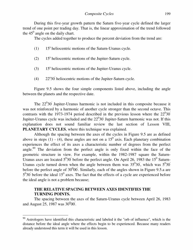
Composite Cycles 199
During this five-year growth pattern the Saturn five-year cycle defined the larger
trend of one point per trading day. That is, the linear approximation of the trend followed
the 450 angle on the daily chart.
The cycles added together to produce the percent deviation from the trend are:
(1) 150 heliocentric motions of the Saturn-Uranus cycle.
(2) 150 heliocentric motions of the Jupiter-Saturn cycle.
(3) 150 heliocentric motions of the Jupiter-Uranus cycle.
(4) 22030' heliocentric motions of the Jupiter-Saturn cycle.
Figure 9.5 shows the four simple components listed above, including the angle
between the planets and the respective date.
The 22030' Jupiter-Uranus harmonic is not included in this composite because it
was not reinforced by a harmonic of another cycle stronger than the second octave. This
contrasts with the 1973-1974 period described in the previous lesson where the 22030'
Jupiter-Uranus cycle was included and the 22030' Jupiter-Saturn harmonic was not. If this
explanation does not sound familiar review the last section of Lesson VIII,
PLANETARY CYCLES, where this technique was explained.
Although the spacing between the axes of the cycles in Figure 9.5 are as defined
above in steps (1) - (4), these angles are not on a 150 axis. Each planetary combination
experiences the effect of its axes a characteristic number of degrees from the perfect
angle.89 The deviation from the perfect angle is only fixed within the face of the
geometric structure in view. For example, within the 1982-1987 square the Saturn-
Uranus axes are located 5030' before the perfect angle. On April 26, 1983 the 150 Saturn-
Uranus cycle turned down when the angle between them was 35030', which was 5030'
before the perfect angle of 30000'. Similarly, each of the angles shown in Figure 9.5.a are
5030' before the ideal 150 axes. The fact that the effects of a cycle are experienced before
the ideal angle is not a problem because;
THE RELATIVE SPACING BETWEEN AXES IDENTIFIES THE
TURNING POINTS.
The spacing between the axes of the Saturn-Uranus cycle between April 26, 1983
and August 25, 1987 was 30000'.
90 Astrologers have identified this characteristic and labeled it the "orb of influence", which is the distance before the ideal angle where the effects begin to be experienced. Because many readers already understood this term it will be used in this lesson.
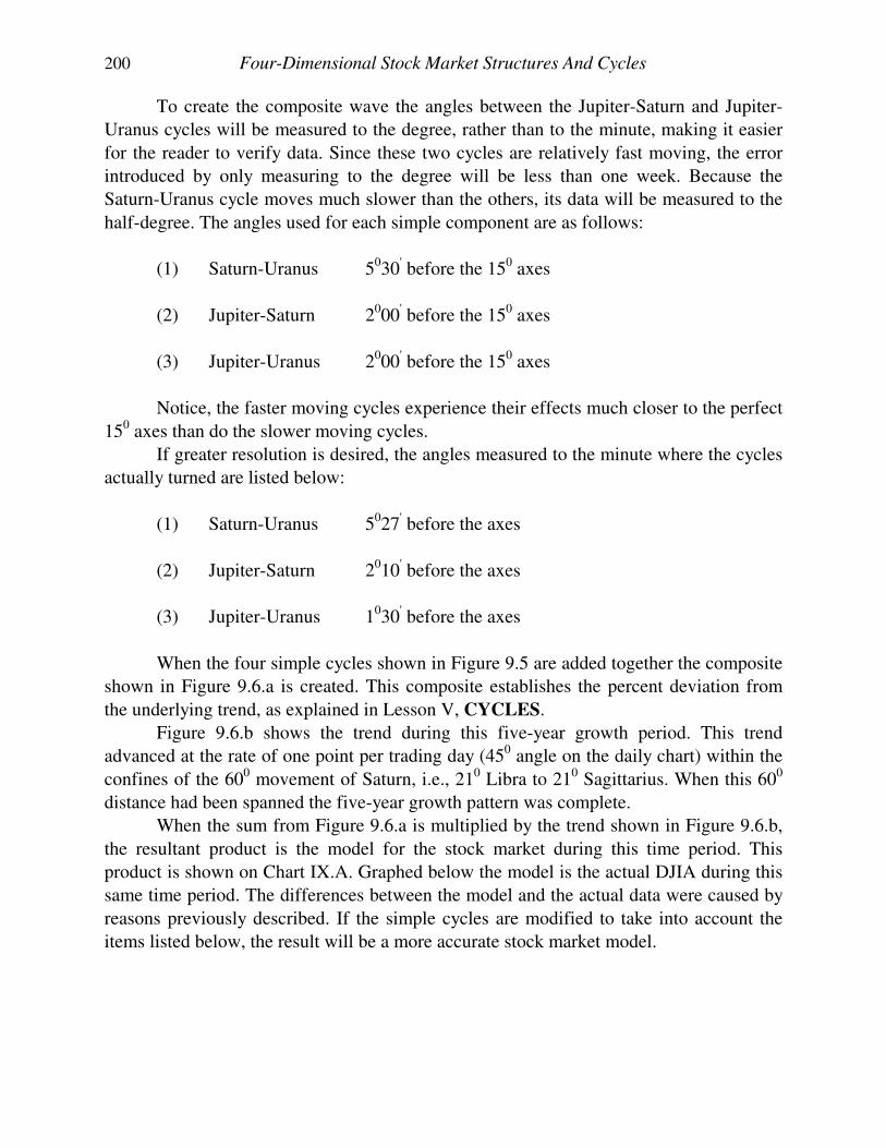
200 Four-Dimensional Stock Market Structures And Cycles
To create the composite wave the angles between the Jupiter-Saturn and Jupiter-
Uranus cycles will be measured to the degree, rather than to the minute, making it easier
for the reader to verify data. Since these two cycles are relatively fast moving, the error
introduced by only measuring to the degree will be less than one week. Because the
Saturn-Uranus cycle moves much slower than the others, its data will be measured to the
half-degree. The angles used for each simple component are as follows:
(1) Saturn-Uranus 5030' before the 150 axes
(2) Jupiter-Saturn 2000' before the 150 axes
(3) Jupiter-Uranus 2000' before the 150 axes
Notice, the faster moving cycles experience their effects much closer to the perfect
150 axes than do the slower moving cycles.
If greater resolution is desired, the angles measured to the minute where the cycles
actually turned are listed below:
(1) Saturn-Uranus 5027' before the axes
(2) Jupiter-Saturn 2010' before the axes
(3) Jupiter-Uranus 1030' before the axes
When the four simple cycles shown in Figure 9.5 are added together the composite
shown in Figure 9.6.a is created. This composite establishes the percent deviation from
the underlying trend, as explained in Lesson V, CYCLES.
Figure 9.6.b shows the trend during this five-year growth period. This trend
advanced at the rate of one point per trading day (450 angle on the daily chart) within the
confines of the 600 movement of Saturn, i.e., 210 Libra to 210 Sagittarius. When this 600
distance had been spanned the five-year growth pattern was complete.
When the sum from Figure 9.6.a is multiplied by the trend shown in Figure 9.6.b,
the resultant product is the model for the stock market during this time period. This
product is shown on Chart IX.A. Graphed below the model is the actual DJIA during this
same time period. The differences between the model and the actual data were caused by
reasons previously described. If the simple cycles are modified to take into account the
items listed below, the result will be a more accurate stock market model.
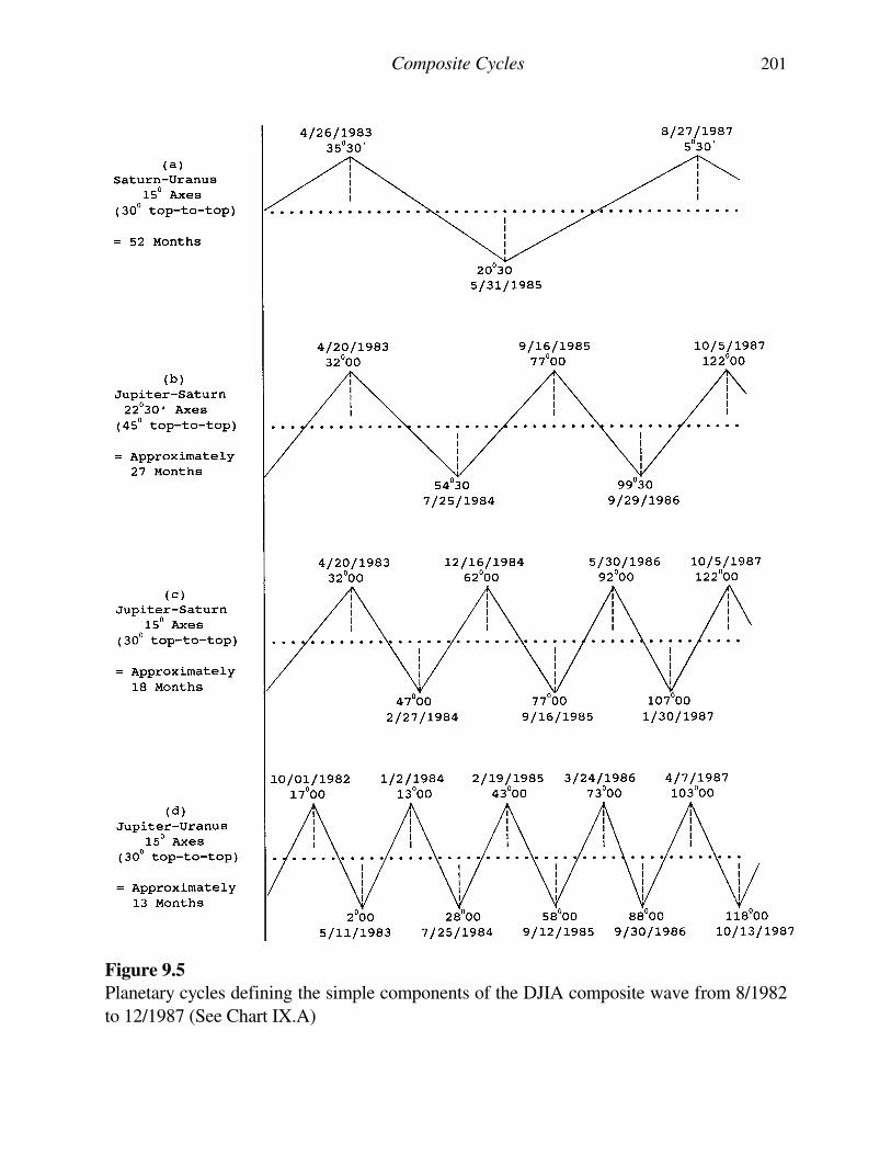
Composite Cycles 201
Figure 9.5
Planetary cycles defining the simple components of the DJIA composite wave from 8/1982
to 12/1987 (See Chart IX.A)
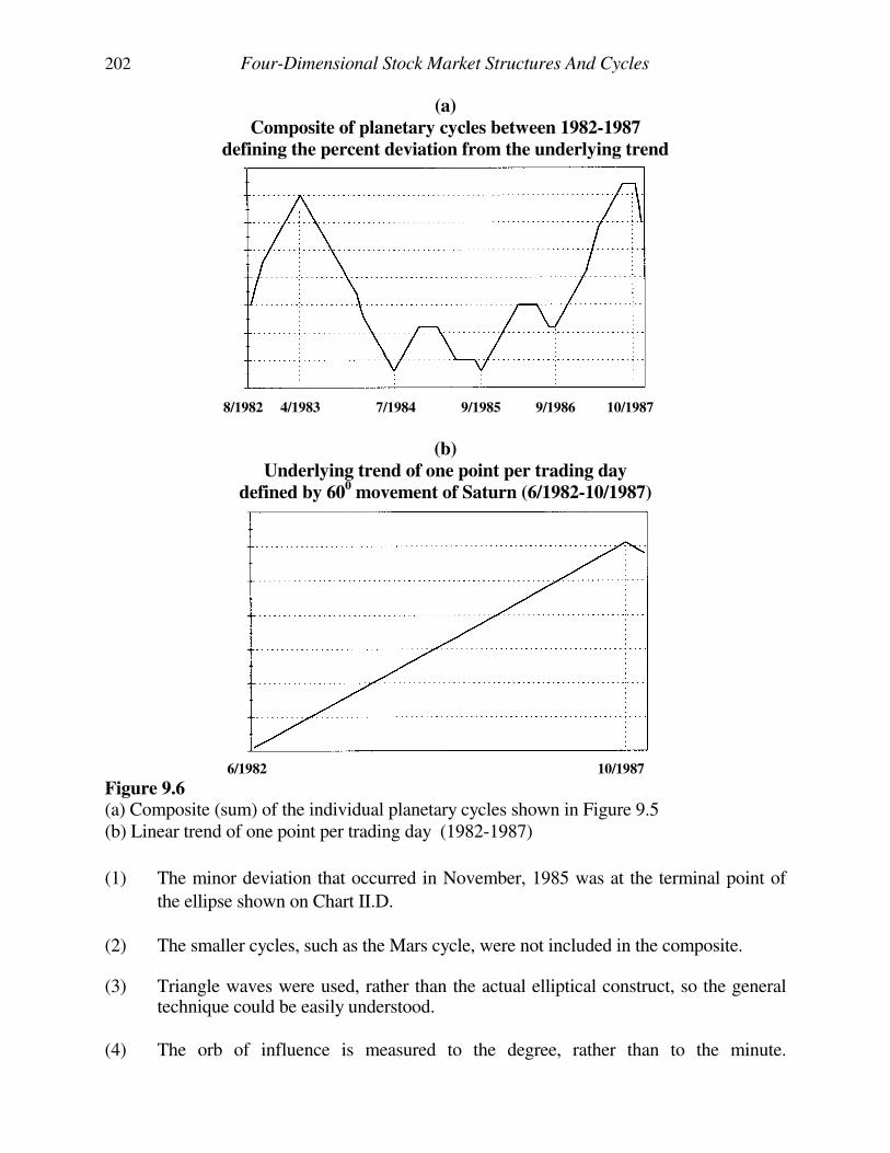
202 Four-Dimensional Stock Market Structures And Cycles
(a)
Composite of planetary cycles between 1982-1987
defining the percent deviation from the underlying trend
8/1982 4/1983 7/1984 9/1985 9/1986 10/1987
(b)
Underlying trend of one point per trading day
defined by 600 movement of Saturn (6/1982-10/1987)
6/1982 10/1987
Figure 9.6 (a) Composite (sum) of the individual planetary cycles shown in Figure 9.5 (b) Linear trend of one point per trading day (1982-1987)
(1) The minor deviation that occurred in November, 1985 was at the terminal point of
the ellipse shown on Chart II.D.
(2) The smaller cycles, such as the Mars cycle, were not included in the composite. (3) Triangle waves were used, rather than the actual elliptical construct, so the general
technique could be easily understood.
(4) The orb of influence is measured to the degree, rather than to the minute.
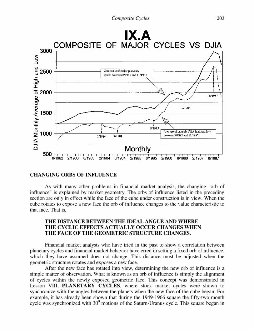
Composite Cycles 203
CHANGING ORBS OF INFLUENCE As with many other problems in financial market analysis, the changing "orb of influence" is explained by market geometry. The orbs of influence listed in the preceding section are only in effect while the face of the cube under construction is in view. When the cube rotates to expose a new face the orb of influence changes to the value characteristic to that face. That is, THE DISTANCE BETWEEN THE IDEAL ANGLE AND WHERE
THE CYCLIC EFFECTS ACTUALLY OCCUR CHANGES WHEN THE FACE OF THE GEOMETRIC STRUCTURE CHANGES.
Financial market analysts who have tried in the past to show a correlation between planetary cycles and financial market behavior have erred in setting a fixed orb of influence, which they have assumed does not change. This distance must be adjusted when the geometric structure rotates and exposes a new face. After the new face has rotated into view, determining the new orb of influence is a simple matter of observation. What is known as an orb of influence is simply the alignment of cycles within the newly exposed geometric face. This concept was demonstrated in Lesson VIII, PLANETARY CYCLES, where stock market cycles were shown to synchronize with the angles between the planets when the new face of the cube began. For example, it has already been shown that during the 1949-1966 square the fifty-two month cycle was synchronized with 300 motions of the Saturn-Uranus cycle. This square began in
204 Four-Dimensional Stock Market Structures And Cycles
1949 when the Saturn-Uranus cycle was at 660. The 660 angle was 60 AFTER the perfect angle of 600. This 60 orb of influence was in effect during the entire 1949-1966 square. During this time each of the axes occurred 60 AFTER the ideal angle, i.e., 660 in 6/1949 (60 after the axis) 960 in 6/1953 (60 after the axis) 1260 in 10/1957 (60 after the axis) 1560 in 6/1962 (60 after the axis) 1730 in 10/1966 (70 after the axis) Chart VIII.G shows the fifty-two month cycle in the DJIA during this time and the corresponding locations of the Saturn-Uranus cycle.
LESSON X
DIMENSIONAL ASPECTS OF TIME
And swear by him that liveth for ever and ever, who created heaven, and the things that therein are, and the earth, and
the things that therein are, and the sea, and the things that are therein, that there should be time no longer.
... Revelation 10:6
INTRODUCTION
The objective of this course has been to increase awareness of the multi-
dimensional reality in which man exists, while at the same time providing practical
applications in the form of financial market timing.
Time has been the common theme underlying each of the preceding lessons. This
lesson will provide a clearer perspective of this elusive concept, allowing the analyst to
better understand what is truly happening in the world around him.
To study the periodic recurrence of mass human behavior, this course used price-
time charts of the stock market, not only because of the availability of recorded historical
data, but also because of the generally inquisitive nature of financial market analysts. The
reader should now realize that applications of the concepts presented in this course
extend well beyond financial markets.
Lesson V, GEOMETRIC STRUCTURES, demonstrated the progressive
evolution of geometric structures as price-time unfolds. To understand the four-
dimensional structures that are unfolded onto two-dimensional price-time charts, it must
be seen how man, as a three-dimensional being, perceives two-dimensional and one-
dimensional objects. The perspective gained by these exercises can then be used to
understand that what man is experiencing at any given time is simply a piece of a
continuum contained in a higher dimension.
Volumes of material can be written on the subject presented in this lesson.
However, the focus will only be on that which clarifies the nature of four-dimensional
stock market structures.
BACKGROUND REVIEW The three dimensions can be represented as shown in Figure 10.1. Each of these figures represents the previous figure set into motion. For example, if the line in Figure 10.1.a is placed into motion it sweeps out the two-dimensional plane shown in Figure 10.1.b. Similarly, if the plane in Figure 10.1.b is placed into motion the three-dimensional cube in Figure 10.1.c is defined. These three figures effectively establish the relationship between motion and changing dimension. That is, as a geometric form in one dimension
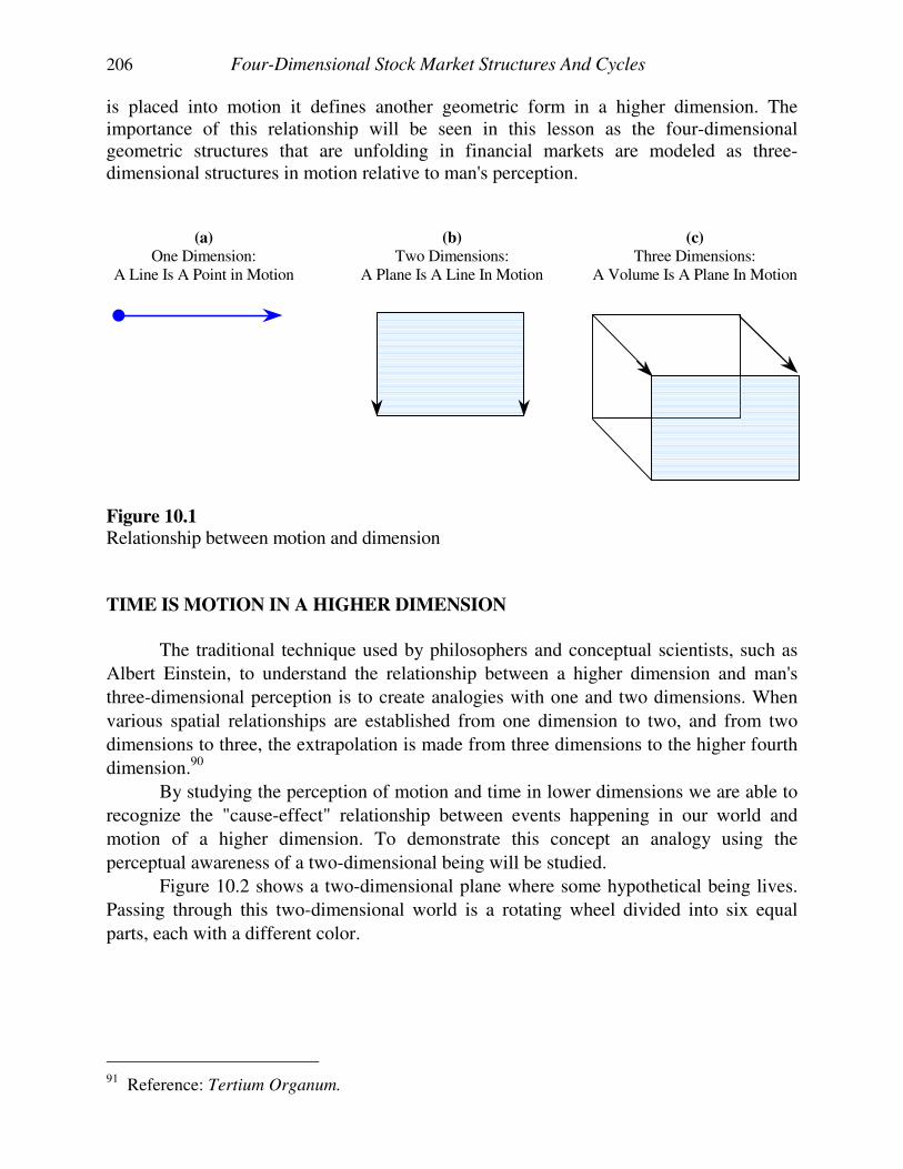
206 Four-Dimensional Stock Market Structures And Cycles
is placed into motion it defines another geometric form in a higher dimension. The importance of this relationship will be seen in this lesson as the four-dimensional geometric structures that are unfolding in financial markets are modeled as three-dimensional structures in motion relative to man's perception.
(a)
One Dimension: A Line Is A Point in Motion
(b)
Two Dimensions: A Plane Is A Line In Motion
(c)
Three Dimensions: A Volume Is A Plane In Motion
Figure 10.1 Relationship between motion and dimension
TIME IS MOTION IN A HIGHER DIMENSION
The traditional technique used by philosophers and conceptual scientists, such as
Albert Einstein, to understand the relationship between a higher dimension and man's
three-dimensional perception is to create analogies with one and two dimensions. When
various spatial relationships are established from one dimension to two, and from two
dimensions to three, the extrapolation is made from three dimensions to the higher fourth
dimension.90
By studying the perception of motion and time in lower dimensions we are able to
recognize the "cause-effect" relationship between events happening in our world and
motion of a higher dimension. To demonstrate this concept an analogy using the
perceptual awareness of a two-dimensional being will be studied.
Figure 10.2 shows a two-dimensional plane where some hypothetical being lives.
Passing through this two-dimensional world is a rotating wheel divided into six equal
parts, each with a different color.
91 Reference: Tertium Organum.
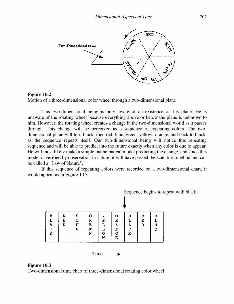
Dimensional Aspects of Time 207
Figure 10.2 Motion of a three-dimensional color wheel through a two-dimensional plane This two-dimensional being is only aware of an existence on his plane. He is unaware of the rotating wheel because everything above or below the plane is unknown to him. However, the rotating wheel creates a change in the two-dimensional world as it passes through. This change will be perceived as a sequence of repeating colors. The two-dimensional plane will turn black, then red, blue, green, yellow, orange, and back to black, as the sequence repeats itself. Our two-dimensional being will notice this repeating sequence and will be able to predict into the future exactly when any color is due to appear. He will most likely make a simple mathematical model predicting the change, and since this model is verified by observation in nature, it will have passed the scientific method and can be called a "Law of Nature". If this sequence of repeating colors were recorded on a two-dimensional chart, it would appear as in Figure 10.3. Sequence begins to repeat with black
Time Figure 10.3 Two-dimensional time chart of three-dimensional rotating color wheel
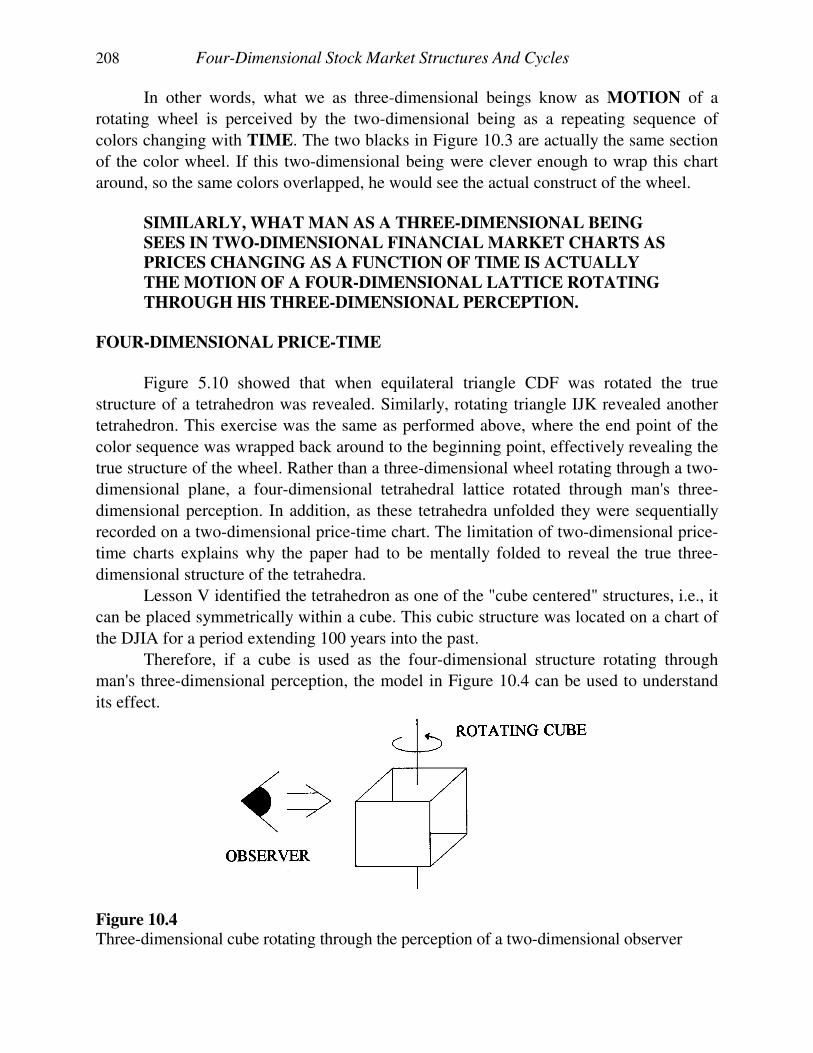
208 Four-Dimensional Stock Market Structures And Cycles
In other words, what we as three-dimensional beings know as MOTION of a
rotating wheel is perceived by the two-dimensional being as a repeating sequence of
colors changing with TIME. The two blacks in Figure 10.3 are actually the same section
of the color wheel. If this two-dimensional being were clever enough to wrap this chart
around, so the same colors overlapped, he would see the actual construct of the wheel. SIMILARLY, WHAT MAN AS A THREE-DIMENSIONAL BEING
SEES IN TWO-DIMENSIONAL FINANCIAL MARKET CHARTS AS
PRICES CHANGING AS A FUNCTION OF TIME IS ACTUALLY
THE MOTION OF A FOUR-DIMENSIONAL LATTICE ROTATING
THROUGH HIS THREE-DIMENSIONAL PERCEPTION.
FOUR-DIMENSIONAL PRICE-TIME
Figure 5.10 showed that when equilateral triangle CDF was rotated the true
structure of a tetrahedron was revealed. Similarly, rotating triangle IJK revealed another
tetrahedron. This exercise was the same as performed above, where the end point of the
color sequence was wrapped back around to the beginning point, effectively revealing the
true structure of the wheel. Rather than a three-dimensional wheel rotating through a two-
dimensional plane, a four-dimensional tetrahedral lattice rotated through man's three-
dimensional perception. In addition, as these tetrahedra unfolded they were sequentially
recorded on a two-dimensional price-time chart. The limitation of two-dimensional price-
time charts explains why the paper had to be mentally folded to reveal the true three-
dimensional structure of the tetrahedra.
Lesson V identified the tetrahedron as one of the "cube centered" structures, i.e., it
can be placed symmetrically within a cube. This cubic structure was located on a chart of
the DJIA for a period extending 100 years into the past.
Therefore, if a cube is used as the four-dimensional structure rotating through
man's three-dimensional perception, the model in Figure 10.4 can be used to understand
its effect.
Figure 10.4 Three-dimensional cube rotating through the perception of a two-dimensional observer
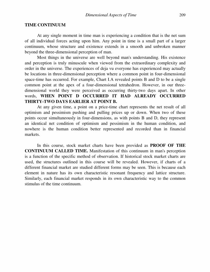
Dimensional Aspects of Time 209
TIME CONTINUUM
At any single moment in time man is experiencing a condition that is the net sum
of all individual forces acting upon him. Any point in time is a small part of a larger
continuum, whose structure and existence extends in a smooth and unbroken manner
beyond the three-dimensional perception of man.
Most things in the universe are well beyond man's understanding. His existence
and perception is truly minuscule when viewed from the extraordinary complexity and
order in the universe. The experiences of deja vu everyone has experienced may actually
be locations in three-dimensional perception where a common point in four-dimensional
space-time has occurred. For example, Chart I.A revealed points B and D to be a single
common point at the apex of a four-dimensional tetrahedron. However, in our three-
dimensional world they were perceived as occurring thirty-two days apart. In other
words, WHEN POINT D OCCURRED IT HAD ALREADY OCCURRED
THIRTY-TWO DAYS EARLIER AT POINT B.
At any given time, a point on a price-time chart represents the net result of all
optimism and pessimism pushing and pulling prices up or down. When two of these
points occur simultaneously in four-dimensions, as with points B and D, they represent
an identical net condition of optimism and pessimism in the human condition, and
nowhere is the human condition better represented and recorded than in financial
markets.
In this course, stock market charts have been provided as PROOF OF THE
CONTINUUM CALLED TIME. Manifestation of this continuum in man's perception
is a function of the specific method of observation. If historical stock market charts are
used, the structures outlined in this course will be revealed. However, if charts of a
different financial market are studied different forms may be seen. This is because each
element in nature has its own characteristic resonant frequency and lattice structure.
Similarly, each financial market responds in its own characteristic way to the common
stimulus of the time continuum.
APPENDIX A
CRASH OF 1987
ANALYSIS OF RETRACEMENT RATIO Many market analysts have incorrectly identified the crash of 1987 as a PHI (1.62)
retracement of the advance from 1982 to 1987. This is an example of the limitation of
one-dimensional analysis. In this case, the analysts are using the single dimension of
price to calculate the retracement. Even if closing values are chosen for the data an
unacceptable error is produced. Using closing values, the advance from 8/12/1982 to 8/25/1987 was: 2722 - 777 = 1945 points To calculate the projected PHI retracement, analysts multiply this advance by 0.618: Projected retracement = 1945 x 0.618 = 1202 points
They then subtract this projected retracement from the high on 8/25/1987 to arrive
at their projected low: Projected low = high in 1987 - projected retracement = 2722 - 1202 = 1520
Even if the intraday low on 10/20/1987 (1616) is used as the actual low, the
projected retracement missed this value by 100 points.
The PTV is used as a means of comparing the results obtained by Fibonacci
analysts, with those obtained by applying the methods in this course.
As calculated in Table 4.1, the PTV from 8/9/1982 to 8/25/1987 was 1994.
Therefore, a perfect 50% retracement would be: Projected retracement = 1994 / 2 = 997
Table 4.1 calculated the actual retracement to be 1013. Therefore, the error
between the projected value and the actual retracement is calculated as follows: 1013 - 997 = 16 = 1.6% 997 997
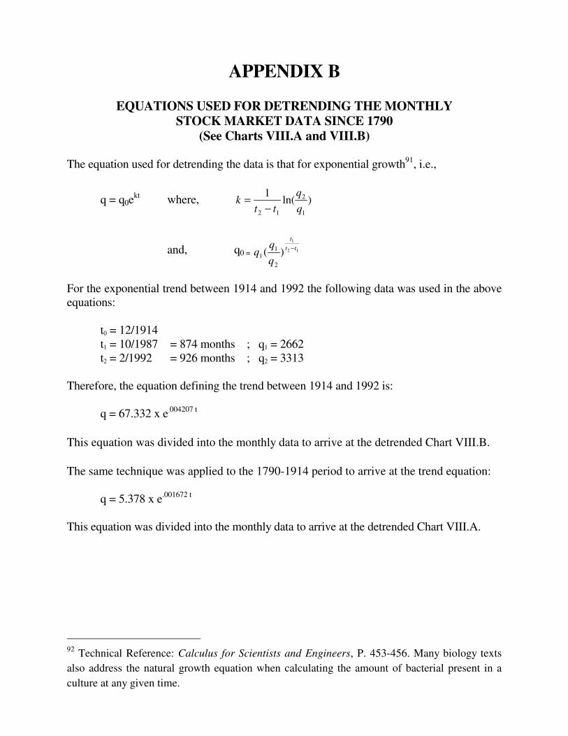
APPENDIX B
EQUATIONS USED FOR DETRENDING THE MONTHLY
STOCK MARKET DATA SINCE 1790
(See Charts VIII.A and VIII.B) The equation used for detrending the data is that for exponential growth91, i.e.,
q = q0ekt where, )ln(
1
1
2
12 q
q
ttk
−=
and, q0 = 12
1
)(2
11
tt
t
q
−
For the exponential trend between 1914 and 1992 the following data was used in the above equations: t0 = 12/1914 t1 = 10/1987 = 874 months ; q1 = 2662 t2 = 2/1992 = 926 months ; q2 = 3313 Therefore, the equation defining the trend between 1914 and 1992 is: q = 67.332 x e.004207 t
This equation was divided into the monthly data to arrive at the detrended Chart VIII.B.
The same technique was applied to the 1790-1914 period to arrive at the trend equation: q = 5.378 x e.001672 t This equation was divided into the monthly data to arrive at the detrended Chart VIII.A.
92 Technical Reference: Calculus for Scientists and Engineers, P. 453-456. Many biology texts
also address the natural growth equation when calculating the amount of bacterial present in a
culture at any given time.
APPENDIX C
W.D. GANN'S ANNUAL FORECASTS
W.D. Gann made available to the public annual forecasts for a variety of financial
markets including stocks and grains. His forecasts for the stock market were well known
for their accuracy, and sold for $100 during the great depression in the 1930's.
Gann shrouded the basis of his forecasts in great secrecy, primarily because of
their simplicity. If the public knew how these forecasts were made they would not have to
pay the high prices for them. This brief writing will identify the basic principle behind
W.D. Gann's annual forecasts. Although there are other considerations that must be taken
into account to fine-tune the forecast, there is a single basic foundation to the approach.
In the introduction to his 1919 stock market forecast Gann stated, "History repeats
itself in the stock market as well as in the lives of men." He also said that he based his
annual forecasts on, "... a time factor which I discovered", and that this time factor was
the basis for his "Master Time Factor".
Simply stated, Gann went back ten and twenty years in the financial market he
was forecasting and used the dates of turning points in those years for his forecast.
The astrological correlations with this time period are successive conjunctions and
oppositions of the Jupiter-Saturn cycle, which occur every ten years.
A copy of Gann's "Forecast of the Stock Market for 1922" is included in Figure
C.1. Below his forecast are one-year graphs of the stock market in 1912 and 1902, which
were ten and twenty years before the year Gann was forecasting.
For all the mystery and price associated with these forecasts and the "Master Time
Factor", it certainly was a simple concept.
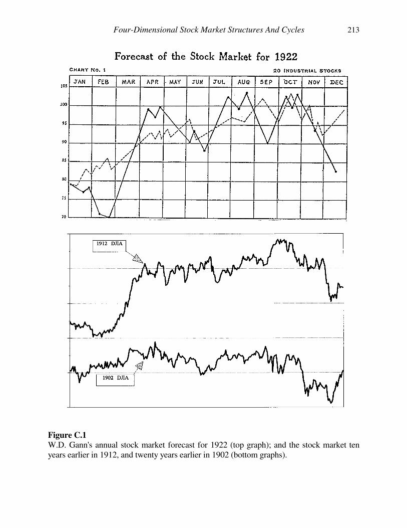
Four-Dimensional Stock Market Structures And Cycles 213
Figure C.1 W.D. Gann's annual stock market forecast for 1922 (top graph); and the stock market ten years earlier in 1912, and twenty years earlier in 1902 (bottom graphs).
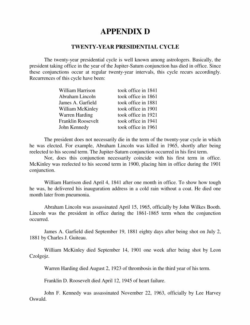
APPENDIX D
TWENTY-YEAR PRESIDENTIAL CYCLE
The twenty-year presidential cycle is well known among astrologers. Basically, the president taking office in the year of the Jupiter-Saturn conjunction has died in office. Since these conjunctions occur at regular twenty-year intervals, this cycle recurs accordingly. Recurrences of this cycle have been: William Harrison took office in 1841 Abraham Lincoln took office in 1861 James A. Garfield took office in 1881 William McKinley took office in 1901 Warren Harding took office in 1921 Franklin Roosevelt took office in 1941 John Kennedy took office in 1961 The president does not necessarily die in the term of the twenty-year cycle in which he was elected. For example, Abraham Lincoln was killed in 1965, shortly after being reelected to his second term. The Jupiter-Saturn conjunction occurred in his first term. Nor, does this conjunction necessarily coincide with his first term in office. McKinley was reelected to his second term in 1900, placing him in office during the 1901 conjunction. William Harrison died April 4, 1841 after one month in office. To show how tough he was, he delivered his inauguration address in a cold rain without a coat. He died one month later from pneumonia. Abraham Lincoln was assassinated April 15, 1965, officially by John Wilkes Booth. Lincoln was the president in office during the 1861-1865 term when the conjunction occurred. James A. Garfield died September 19, 1881 eighty days after being shot on July 2, 1881 by Charles J. Guiteau. William McKinley died September 14, 1901 one week after being shot by Leon Czolgojz. Warren Harding died August 2, 1923 of thrombosis in the third year of his term. Franklin D. Roosevelt died April 12, 1945 of heart failure. John F. Kennedy was assassinated November 22, 1963, officially by Lee Harvey Oswald.
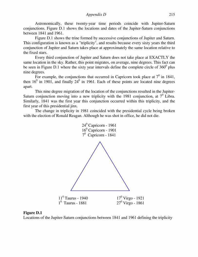
Appendix D 215
Astronomically, these twenty-year time periods coincide with Jupiter-Saturn conjunctions. Figure D.1 shows the locations and dates of the Jupiter-Saturn conjunctions between 1841 and 1961. Figure D.1 shows the trine formed by successive conjunctions of Jupiter and Saturn. This configuration is known as a "triplicity", and results because every sixty years the third conjunction of Jupiter and Saturn takes place at approximately the same location relative to the fixed stars. Every third conjunction of Jupiter and Saturn does not take place at EXACTLY the same location in the sky. Rather, this point migrates, on average, nine degrees. This fact can be seen in Figure D.1 where the sixty year intervals define the complete circle of 3600 plus nine degrees. For example, the conjunctions that occurred in Capricorn took place at 70 in 1841, then 160 in 1901, and finally 240 in 1961. Each of these points are located nine degrees apart. This nine degree migration of the location of the conjunctions resulted in the Jupiter-Saturn conjunction moving into a new triplicity with the 1981 conjunction, at 70 Libra. Similarly, 1841 was the first year this conjunction occurred within this triplicity, and the first year of this presidential jinx. The change in triplicity in 1981 coincided with the presidential cycle being broken with the election of Ronald Reagan. Although he was shot in office, he did not die. 240 Capricorn - 1961 160 Capricorn - 1901 70 Capricorn - 1841 110 Taurus - 1940 170 Virgo - 1921 10 Taurus - 1881 270 Virgo - 1861
Figure D.1 Locations of the Jupiter-Saturn conjunctions between 1841 and 1961 defining the triplicity
APPENDIX E
FORMAT OF DATA AND TABLES USED IN THIS COURSE
FORMAT OF STOCK MARKET DATA
The price values used in calculations in this course are intraday high and low Dow
Jones Industrial Averages. The time values are when the hourly highs and lows occurred,
as recorded in the Wall Street Journal. Using intraday values instead of hourly readings
allows greater accuracy, since large price swings can occur between two hourly readings.
This method will introduce a certain amount of error. However, the availability of long-
term historical data in the intraday format makes this approach the most accurate for the
given data.
Also, since the Dow Jones Industrial Averages is a non-homogeneous index
composed of a variety of stocks, each vibrating at its own characteristic frequency, this
index does not produce as accurate results as would be achieved using a single stock or
commodity. However, once again, the availability of long-term historical data (or lack of)
is a consideration here. This approach makes more sense as vibration rates lasting for
several decades and extending back in time into the eighteenth century are studied.
FORMAT OF TABLES USED IN THIS COURSE
Tables are used extensively throughout this course to display all data used in
calculations. This allows the skeptical reader to independently verify conclusions.
Almost all the tables in Part I contain data used to calculate PTVs. The format of
all these tables is the same. Each row contains the data for one PTV. The eight columns
contain the data used for the calculation of each of the PTVs, and are structured as
follows:
First column - "Price-Time radius vector" lists the letters identifying the
PTV from the chart identified in the table header.
Second column - "Date & Time of High" gives the date and time of day the
highest price was reached. This may be the beginning or the end point of the PTV, depending upon whether the PTV was descending or ascending, respectively.
Third column - "Price High" gives the value of the highest price reached by
the PTV. This value is reached on the date listed in the second column of the table. If the PTV is measured between two bottoms the value in the third column will be the INTRADAY LOW on the date listed in the second column.
Appendix E 217
For all other situations the value in this column will be the INTRADAY HIGH on the date listed in the second column.
An example where the high value for the PTV is an
intraday low is seen on Chart I.A with PTV CF. Point F is the
high point for the PTV. However, since point F is a bottom,
the price high used to calculate CF is the intraday low on the
date at point F. Fourth column - "Date & Time of Low" gives the date and time of day the
lowest price was reached. This may be the beginning or the end point of the PTV, depending upon whether the PTV was ascending or descending, respectively.
Fifth column - "Intraday Low" gives the value of the PTV price low reached
on the date listed in the fourth column. If the PTV is measured between two tops the value in this column will be the INTRADAY HIGH on the date listed in the fourth column. For all other situations the value in this column will be the INTRADAY LOW on the date listed in the fourth column.
Sixth column - "Time Change (in hours)" gives the total trading hours that
elapsed between the date of the high and low, as listed in the second and fourth columns.
Seventh column - "Price Change (points)" gives the total change in price that
occurred between the high and low, i.e., the value listed in the third column minus the value listed in the fifth column.
Eighth Column - "Vector Value (PTV)" uses the values from column six and
column seven to calculate the PTV, as described in Figure 1.1.
The tables in Part II have a variety of formats. When planetary cycles are being
studied the first column lists the beginning and ending dates of the related stock market
cycle. The second and third columns list the heliocentric locations of the associated
planet on the dates listed in the first column. The final column subtracts the second and
third column, giving the total distance traveled by the planet between the dates listed in
the first column.
APPENDIX F
URANUS CYCLE AND THE PERIODICITY OF AMERICAN WAR
Volumes of material can be written on the subject of the periodicity of war.
However, because of limited space this writing will only serve as a general introduction
to the subject. The focus will be on the correlation between the Uranus quarter-cycle and
American war.
Gemini is the "ruling sign" of the United States, as defined by the locations of the
planets at its birth. Also, Uranus is know as the "revolutionary planet", causing disruption
and war. This discussion will show that the Uranus quarter-cycle of 21 years corresponds
with war in this country.
The three most significant wars in American history in terms of affecting the form
of government and the relative number of lives lost have been:
(1) The Revolutionary War officially began with the signing of the Declaration
of Independence on July 4, 1776. This date defined the birth of the United
States.
(2) The Civil War officially began on April 12, 1861 with the firing on Fort
Sumter. This date was one Uranus cycle (84 years 9 months) after the
signing of the Declaration of Independence in 1776.
(3) World War II ended in Europe on April 30, 1945 when Adolf Hitler
committed suicide. This date was one Uranus cycle (84 years) after the start
of the Civil War in 1861 and two Uranus cycles after the signing of the
Declaration of Independence in 1776.
The three major wars listed above coincided with Uranus returning to the same
location in the heavens.
Figure F.1 shows the location of Uranus during each of the major wars in the
United States. Since the birth of the United States in 1776, Uranus has entered Gemini
three times. These dates are shown on the bottom of Figure F.1. When the Declaration of
Independence was signed in 1776 Uranus was at 100 Gemini. At the beginning of the
Civil War in 1861 Uranus was at 110 Gemini. Similarly, the end of World War II in 1945
coincided with Uranus arriving at 120 Gemini. Notice that this area in the Uranus cycle
was also identified in Lesson VIII as stock market nodal points, shown on Charts VIII.A
and VIII.B. Uranus will again return to this location in the year 2029, which also coincides with the 45-year Saturn-Uranus cycle returning to its same location as at the stock market nodal point in 1982.
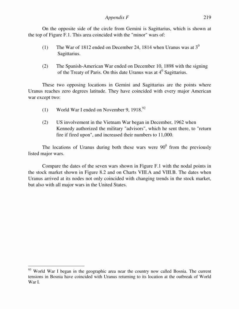
Appendix F 219
On the opposite side of the circle from Gemini is Sagittarius, which is shown at
the top of Figure F.1. This area coincided with the "minor" wars of:
(1) The War of 1812 ended on December 24, 1814 when Uranus was at 30
Sagittarius.
(2) The Spanish-American War ended on December 10, 1898 with the signing
of the Treaty of Paris. On this date Uranus was at 40 Sagittarius.
These two opposing locations in Gemini and Sagittarius are the points where
Uranus reaches zero degrees latitude. They have coincided with every major American
war except two:
(1) World War I ended on November 9, 1918.92
(2) US involvement in the Vietnam War began in December, 1962 when
Kennedy authorized the military "advisors", which he sent there, to "return
fire if fired upon", and increased their numbers to 11,000.
The locations of Uranus during both these wars were 900 from the previously
listed major wars.
Compare the dates of the seven wars shown in Figure F.1 with the nodal points in
the stock market shown in Figure 8.2 and on Charts VIII.A and VIII.B. The dates when
Uranus arrived at its nodes not only coincided with changing trends in the stock market,
but also with all major wars in the United States.
93 World War I began in the geographic area near the country now called Bosnia. The current tensions in Bosnia have coincided with Uranus returning to its location at the outbreak of World War I.
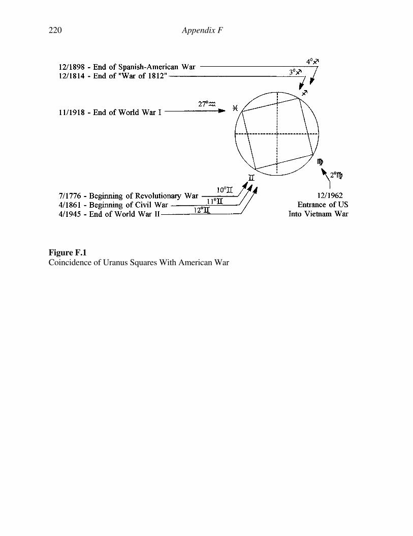
220 Appendix F
Figure F.1 Coincidence of Uranus Squares With American War
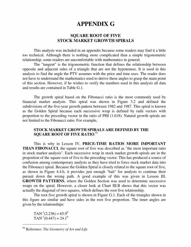
APPENDIX G
SQUARE ROOT OF FIVE
STOCK MARKET GROWTH SPIRALS This analysis was included in an appendix because some readers may find it a little too technical. Although there is nothing more complicated than a simple trigonometric relationship, some readers are uncomfortable with mathematics in general. The "tangent" is the trigonometric function that defines the relationship between opposite and adjacent sides of a triangle that are not the hypotenuse. It is used in this analysis to find the angle the PTV assumes with the price and time axes. The reader does not have to understand the mathematics used to derive these angles to grasp the main point of this section. However, if he wishes to verify the numbers used in this analysis all data and results are contained in Table G.1. The growth spiral based on the Fibonacci ratio is the most commonly used by financial market analysts. This spiral was shown in Figure 3.2 and defined the subdivisions of the five-year growth pattern between 1982 and 1987. This spiral is known as the Golden Spiral because each successive wrap is defined by radii vectors with proportion to the preceding vector in the ratio of PHI (1.618). Natural growth spirals are not limited to the Fibonacci ratio. For example,
STOCK MARKET GROWTH SPIRALS ARE DEFINED BY THE SQUARE ROOT OF FIVE RATIO.93
This is why in Lesson IV, PRICE-TIME RATIOS MORE IMPORTANT
THAN FIBONACCI, the square root of five was described as "the most important ratio in stock market analysis". Each successive wrap in stock market growth spirals are in the proportion of the square root of five to the preceding vector. This has produced a source of confusion among contemporary analysts as they have tried to force stock market data into the Fibonacci spiral. Because the Golden Spiral is closely related to the square root of five, as shown in Figure 4.4.b, it provides just enough "bait" for analysts to continue their pursuit down the wrong path. A good example of this was given in Lesson III, GROWTH PATTERNS, where the Golden Section was used to determine successive wraps on the spiral. However, a closer look at Chart III.B shows that this vector was actually the diagonal of two squares, which defines the root five relationship. The root five growth spiral is shown in Figure G.1. Each of the triangles shown in this figure are similar and have sides in the root five proportion. The inner angles are given by the relationships: TAN-1(2.236) = 65.90 TAN-1(0.447) = 24.10
94 Reference: The Geometry of Art and Life.
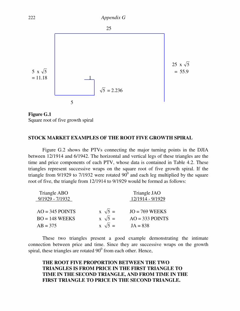
222 Appendix G
25
25 x 5
5 x 5 = 55.9
= 11.18 1
5 = 2.236
5
Figure G.1 Square root of five growth spiral
STOCK MARKET EXAMPLES OF THE ROOT FIVE GROWTH SPIRAL
Figure G.2 shows the PTVs connecting the major turning points in the DJIA
between 12/1914 and 6/1942. The horizontal and vertical legs of these triangles are the
time and price components of each PTV, whose data is contained in Table 4.2. These
triangles represent successive wraps on the square root of five growth spiral. If the
triangle from 9/1929 to 7/1932 were rotated 900 and each leg multiplied by the square
root of five, the triangle from 12/1914 to 9/1929 would be formed as follows: Triangle ABO Triangle JAO 9/1929 - 7/1932 12/1914 - 9/1929
AO = 345 POINTS x 5 = JO = 769 WEEKS
BO = 148 WEEKS x 5 = AO = 333 POINTS
AB = 375 x 5 = JA = 838
These two triangles present a good example demonstrating the intimate
connection between price and time. Since they are successive wraps on the growth
spiral, these triangles are rotated 900 from each other. Hence, THE ROOT FIVE PROPORTION BETWEEN THE TWO
TRIANGLES IS FROM PRICE IN THE FIRST TRIANGLE TO
TIME IN THE SECOND TRIANGLE, AND FROM TIME IN THE
FIRST TRIANGLE TO PRICE IN THE SECOND TRIANGLE.
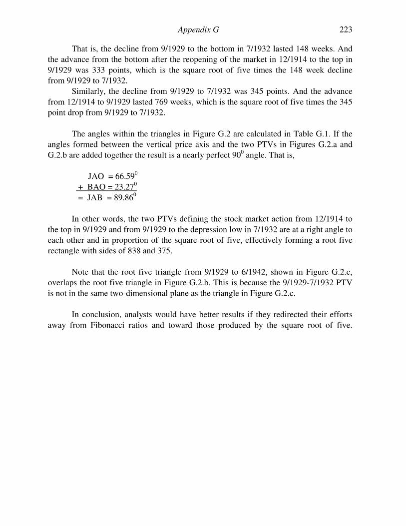
Appendix G 223
That is, the decline from 9/1929 to the bottom in 7/1932 lasted 148 weeks. And
the advance from the bottom after the reopening of the market in 12/1914 to the top in
9/1929 was 333 points, which is the square root of five times the 148 week decline
from 9/1929 to 7/1932.
Similarly, the decline from 9/1929 to 7/1932 was 345 points. And the advance
from 12/1914 to 9/1929 lasted 769 weeks, which is the square root of five times the 345
point drop from 9/1929 to 7/1932.
The angles within the triangles in Figure G.2 are calculated in Table G.1. If the
angles formed between the vertical price axis and the two PTVs in Figures G.2.a and
G.2.b are added together the result is a nearly perfect 900 angle. That is,
JAO = 66.590
+ BAO = 23.270
= JAB = 89.860
In other words, the two PTVs defining the stock market action from 12/1914 to
the top in 9/1929 and from 9/1929 to the depression low in 7/1932 are at a right angle to
each other and in proportion of the square root of five, effectively forming a root five
rectangle with sides of 838 and 375.
Note that the root five triangle from 9/1929 to 6/1942, shown in Figure G.2.c,
overlaps the root five triangle in Figure G.2.b. This is because the 9/1929-7/1932 PTV
is not in the same two-dimensional plane as the triangle in Figure G.2.c.
In conclusion, analysts would have better results if they redirected their efforts
away from Fibonacci ratios and toward those produced by the square root of five.
224 Appendix G
Table G.1
Angles of PTVs in Figure G.2 Relative to the Price and Time Axes
(Price and Time Values in Middle Column are From Table 4.2)
Angle
In Figure G.2
Opposite Side /
Adjacent Side
TAN-1
of
Opposite / Adjacent
From Preceding Column
AJO in Figure G.2.a 333 Points = 0.43 769 Weeks
TAN-1(0.43) = 23.270
JAO in Figure G.2.a 769 Weeks = 2.31 333 Points
TAN-1(2.31) = 66.590
BAO in Figure G.2.b 148 Weeks = 0.43 345 Points
TAN-1(0.43) = 23.270
ABO in Figure G.2.b 345 Points = 2.33 148 Weeks
TAN-1(2.33) = 66.780
CAO in Figure G.2.c 659 Weeks = 2.25 293 Points
TAN-1(2.25) = 66.030
ACO in Figure G.2.c 293 Points = 0.44 659 Weeks
TAN-1(0.44) = 23.750
(a) (b) (c) A 9/1929 9/1929 9/1929 A A J O O B O C 12/1914 7/1932 6/1942 Figure G.2 Similar triangles formed by PTVs between 1914 – 1942
REFERENCES
The books used as references in both the “Technical Reference” and “Reference” footnotes are listed below. Some of these are college level science and engineering texts which require some technical background to fully understand. Others require no previous training.
American Heliocentric Ephemeris 1901-2000, Neil Michelsen, (1982), Astro Computing Services, ISBN 0-917086-36-8 Calculus With Analytic Geometry, Munem & Foulis, (1978), Worth Publishers, ISBN 0-87901-087-8 Chaos, James Gleik Chemical Principles, Dickerson, Gray, Darensbourg, (1970), Benjamin/Cummings Publishing, ISBN 0-8053-2422-4 Chemistry, Reactions, Structure, and Properties, Dillard & Goldberg, (1978) MacMillan Publishing, ISBN 0-02-329580-5
Connections – The Geometric Bridge Between Art and Science, Jay Kappraff, (1990), McGraw-Hill, ISBN 0-07-034251-2 Curves of Life, Theodore Andrea Cook, (1979), Dover Publications, ISBN 0-486-23701-X Cycles, Dewey, (1971), Hawthorn Books, Library of Congress 70-130730 Electronic Devices and Circuit Theory, Boylestad & Nashelsky, (1978), Prentice-Hall, ISBN 0-13-250340-9 Elements of Dynamic Symmetry, Jay Hambridge Engineering Circuit Analysis, Hayt & Kemmerly, (1978), McGraw-Hill, ISBN 0-07-027393-6 Feedback and Control Systems, (1967), Stefano, Stubberud, Williams, McGraw-Hill Fundamentals of Physics – Extended, Halliday, Resnick, Wakler, (1997), John Wiley, ISBN 0-471-10559-7 Geometry of Art and Life, Matila Ghyka, (1977), Dover Publications, ISBN 0-486-23542-4 Introduction to Physics for Scientists and Engineers, Bueche, (1969), McGraw-Hill, ISBN 0-07-008871-3 Kepler’s Geometrical Cosmology, (1988), J.V. Field, University of Chicago Press, ISBN 0-226-24823-2 Modern Control Systems, Doft, (1980), Addison-Wesley, ISBN 0-201-01258-8 Modern Physics, Gautreau & Savin, (1978), McGraw-Hill, ISBN 0-07-023062-5 Sacred Geometry, Robert Lawlor, (1989), Thames & Hudson, ISBN 0-500810303 Tertium Organum, Petyr Demianovich Ouspensky
BOOKS AND SOFTWARE BY THIS AUTHOR
Please visit www.cycle-trader.com for details on any of these books.
Pentagonal Time Cycle Theory
Cowan's latest book published in 2009.
Four-Dimensional Stock Market Structures And Cycles
The first ten lessons of this series are contained within these two books. Lessons
one through five deal with the four-dimensional geometric structures in financial
markets. The last five lessons identify the cycles correlated with turning points
within these structures. These cycles are applicable to any market.
Market Science Volume I - Square Of Twelve
This book contains lessons eleven and twelve and proves that the square of twelve
is the elemental unit of measurement within the soybean market.
XI - Square Of Twelve
XII - Vectorial Partitioning
Market Science Volume II - Market Dynamics
This book contains lessons thirteen through sixteen and an update on stock market
cycles and the growth spiral unfolding in that market, as of July 1995.
XIII - Non-Euclidean Price-Time Geometry
XIV - Quantum Energy Levels Of Freely Traded Markets
XV - Soybean Cycles
XVI - Square Of Fifty-Two
Also - Stock Market Cycle Update And Current Growth Spiral
Also - Applications Of The Musical Fifth To Timing
Also - Dimensions Of Ancient Monuments And Soybean Spirals
W.D. Gann Commodity Trading Courses – Edited by Bradley F. Cowan
W.D. Gann Stock Market Trading Courses – Edited by Bradley F. Cowan
The Rare Writings Of W.D. Gann – Edited by Bradley F. Cowan
CycleTimer Software – Automates Many of the Techniques Used in This Book
Stock Market Geometry; P.O. Box 9756; San Diego, CA 92169-0756 USA


![HSK Level 4123 3 词语 [cíy ]ǔ обороты речи; выражения 方言词语 [fāngyán cíy ] — диалектизм ǔ 124 2 次 [cì] следующий; второй;](https://static.documents.pub/doc/80x56/5f7603acb9264e5d6f5a32b4/hsk-level-4-123-3-ee-cy-eee.jpg)


![Ô èy D Ô¢Ú£ Ô èy D Ô¢ T£{ >y S ¢©£¢ S qy & ºJ«æÇ¿«£ " ñ,]O P O ± É ´ñ èµÍ Ä ÖÃÄÀwq Ýq] J j >y¾ ¢ ñ,] É ´© È W ^q£ " ®~sy` & É ´±Ù ÄÉ¿Äë](https://static.documents.pub/doc/80x56/5ed071e8df2da27dae75dd6b/-y-d-y-d-t-y-s-s-qy-j.jpg)

