MPRAMunich Personal RePEc Archive

Lucas Paradox in the Short-Run

Bilal Keskinsoy

Anadolu University

25 April 2017

Online at https://mpra.ub.uni-muenchen.de/78783/MPRA Paper No. 78783, posted 28 April 2017 13:39 UTC

1

Lucas Paradox in the Short-Run

Bilal Keskinsoy

Anadolu University Department of Economics, IIBF Building, Tepebaşı

26210 Eskişehir/TURKEY bilalkeskinsoy@gmail.com

Abstract

This paper is concerned with whether the persistence of the Lucas paradox (that unlike

what the classical economic theory would predict, capital flows to richer economies rather

than poorer ones where marginal returns to capital are expected to be higher) within

developing countries is because of the unobservable county-specific effects. Perhaps capital

has been flowing to where it has already flowed and not necessarily where it had already

been. Using five-year (rolling-averaged) panel data for up to 47 developing countries over the

period 1980-2006, it examines if including the institutional quality index removes the Lucas

paradox intertemporally (i.e. in the short-run). The ‘short-run’ relationships are captured by

employing linear static (principally within-group fixed effects) and dynamic (system GMM)

panel data methods. I demonstrate that the persistence in the Lucas paradox within

developing countries is so entrenched that allowing for unobserved country-specific effects,

within-group (time series) variation and autoregressive dynamics do not resolve the paradox.

Keywords: Capital flows, Lucas paradox, Institutional quality, Economic growth, Within-

group fixed effects, System GMM

JEL classification: E02, F20, F41, G15, J24, O16

2

1. Introduction

Ordinary least squares (OLS) estimators using time-aggregated (long-term averaged) data

for cross-sections are charged not to take the intertemporal dependence into account but fit

mainly long-run steady-state equilibrium models (Cameron and Trivedi, 2005, Sinn, 1992).

In such cross-section models, the unobservable country-specific fixed effects that are

correlated with the observed characteristics (i.e. explicitly controlled variables) included in

the model can cause statistical difficulties in estimation: potential aggregation bias, loss of

information (due to absorbed time variation), inconsistency and inefficiency. Neither can they

account for the causes of behavioural persistence since they are unable to control for true

state dependence (autoregressivity, especially in the dependent variable).1

Drawing largely on the theoretical considerations in Keskinsoy (2017), this paper

addresses the methodological and measurement issues discussed above. It is concerned with

the question: Is it (the persistence of the Lucas paradox within developing countries, as

documented in Keskinsoy, 2017) because of the unobservable county-specific effects or is it

actually due to the persistence of the capital in flowing to a certain market but appears as if its

initial abundance in that market spurs further inflows? In other words, perhaps capital has

been flowing to where it has already flowed and not necessarily where it had already been.

Using five-year (rolling-averaged) panel data for up to 47 developing countries over the

period 1980-2006, it examines if including the institutional quality index removes the Lucas

paradox intertemporally (i.e. in the short-run). The ‘short-run’ relationships are captured by

employing linear static (principally within-group fixed effects) and dynamic (system GMM)

panel data methods (Pesaran and Smith, 1995, Houthakker, 1965, Baltagi and Griffin, 1984).2

In this paper, I additionally investigate the short-run prognoses of Acemoglu and Zilibotti

(1997) who, in contrast to Lucas (1988, 1990), argue that economic growth, development and

capital flow patterns are predicted by a neoclassical growth model augmented with

assumptions of micro-level indivisibilities and uncertainty. According to their overlapping

generations model of optimal portfolio choice, it is not a paradox at all (as it is already

expected) that more foreign capital will flow to richer economies in the short-run. The data

and methodology employed here enable such an empirical verification. Capital inflows per

1 In a time series context, state dependence means that state at a given moment depends on the previous state(s) of the system.

2 Baltagi (2005) states that the between estimator (pooled OLS or equivalently cross-section OLS, which are based on the cross-section component of the data) tends to give long-run estimates while the within estimator (which is based on the time-series component of the data) tends to give short-run estimates.

3

capita (the dependent variable as the sum of foreign direct and portfolio equity investment)

represent the cross-border risky financial investments in Acemoglu and Zilibotti (1997). The

initial endowments were captured by the initial GDP per capita while the risk-return trade-off

(insurance, investment security or risk conditions) is embodied in the institutional quality

variable. Static and dynamic panel estimators that fit to ‘time �’ notion let us analyse the

short-run or dynamic implications of their model. Comprehensive review of the derivation of

Acemoglu and Zilibotti (1997) results that are particularly considered here is in the appendix.

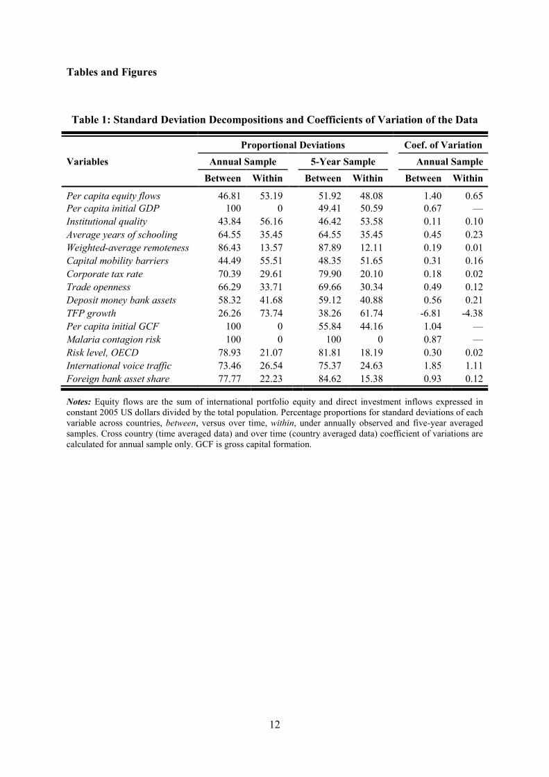
[Table 1]

To compare space (between) and time (within) variations in the data, coefficients of

variation and percentage proportions for standard deviations of over-time and cross-country

averaged data are given in Table 1. Notwithstanding the fact that between coefficients of

variation are larger for all variables, standard deviation proportions are either relatively close

to each other or even higher in within cases for, at least, the first three most important

variables. All in all, the figures in the table imply that time variation should not be ignored as

incorporating time dimension through appropriate model specifications would not only

alleviate aggregation bias but would also yield significant information and efficiency gains.

Figure 1 shows per capita equity flows by subperiods. During the first two decades capital

flows follow steadily declining trajectory and starting 1990s onwards the trend reverses in the

direction of increase.

[Figure 1]

The rest of the paper proceeds as follows. Econometric methodology is devised in Section

2. Section 3 overviews the descriptive statistics and pairwise correlations. Results from static

panel estimators are examined in Section 4, while dynamic panel regressions discussed in

Section 5. Section 6 concludes.

2. Methodology

Given small �, relative to �, I avail of cross-section asymptotics in building up the

following sections.3

3 � → ∞ asymptotics are more appropriate than � → ∞ asymptotics, even though � is practically fixed while �

can grow (Wooldridge, 2002). This is in fact the case in my country panel study. Nonetheless, if � is

sufficiently large relative to � and one can assume rough independence in the cross section or make sure it to be so by introducing cluster robust estimators then the suitable approximations warranted (Ibid.).

4

2.1 Specification for Static Panel Estimators

The static two-way error components population regression function for sample

estimations can be written as:

��� = + � �� + ����+ ��� � = 1,… ,�; � = 1,… , � (1)

where ��� is the dependent variable (five-year averaged inflows of portfolio equity and

foreign direct investment expressed as capital inflows per capita) for country � and time

period �, is a constant, �� is the main regressor (the natural log of GDP per capita at first

years of each panels), ��� is a 1 × (� − 1) row vector of any additional explanatory

variables. The estimators of interest are the scalar � and (� − 1) × 1 column vector �;

� ≥ 1 being the number of covariates. �� will be capturing the Lucas paradox and �� the

influence of the other regressors on capital inflows (and whether they account for, that is

remove, the paradox). Assuming ���, the composite disturbances, follow a generalized two-

way error components structure

��� = �� + � + !��� = 1,… ,�; � = 1,… , � (2)

where �� refers to country specific unobservable fixed effects, � denotes period-specific

effects which are assumed to have fixed parameters to be estimated as coefficients of time

dummies, and !�� denotes idiosyncratic errors.

Each of the three static panel data models (pooled OLS, fixed effects and random effects)

applied specifies different orthogonality, rank and efficiency assumptions about the elements

of ��� and ��� in terms of conditional expectations, invertibility and variances. Pooled OLS

(POLS) assumes that �� is fixed over time and has a constant partial impact on the mean

response in each time period. If �� is correlated with any element of ���, then POLS estimator

is biased and inconsistent. Because POLS does not offer any solution for potential cross

section heterogeneity I consider two other estimators. Fixed effects model (FEM) allows for

arbitrary correlation between �� and ��� by relaxing the orthogonality assumption and deals

with this through within transformation; time demeaning of Equation (1) removes observed

and unobserved fixed effects. More intuitively, FEM accounts for unobserved country effects

that are correlated with ��� but ‘sweeps up’ time-invariant variables. On the other hand,

random effects model (REM) involves generalized least squares (GLS) transformation under

stricter orthogonality assumptions. REM estimator is obtained by quasi time demeaning

which implies the removal of only a pre-estimated fraction of the time averages. Having the

5

advantage of explicitly allowing for time-invariant variables REM favoured over FEM if

country effects are uncorrelated with ��� but is inconsistent if FEM is the true model. It is

standard to choose between FEM and REM using a cross section-time series adapted version

of the Hausman specification test. To avoid heteroscedasticity and serial correlation in !�� I employ the Huber/White/sandwich cluster robust estimator.

2.2 Representation of Dynamic Panel Estimators

As many economic relationships are inherently dynamic (Nerlove, 2002), the dynamics of

adjustment can be represented by a dynamic two-way error components population

regression:

��� = + "��#$% + � �� + ���� + ���� = 1,… ,�; � = 1, … , �; & = 1, 2 (3)

where "��#$ is the vector containing the lags of the dependent variable (capital inflows per

capita) as regressors rendering (3) to include an autoregressive process. The parameter vector

% involves the scalars measuring the extent of state dependence (inertia), and the composite

disturbance term is similarly specified as a two-way error components mechanism

��� = �� + � + !��� = 1,… ,�; � = 1,… , � (4)

where �� represents, as before, state-specific effects, and � denotes period-specific effects

which are assumed to have fixed parameters to be estimated as coefficients of time dummies.

In a dynamic specification of the kind in (3) POLS, within-group FEM, and REM do not

take the endogeneity of the lagged dependent variable into consideration and produce biased

and inconsistent estimates. Therefore, a generalized method of moments (GMM) approach is

required. Because my short time panel data are highly persistent I use the Blundell and Bond

(1998) system GMM estimator which entails contemporaneous first differences to instrument

the levels of the endogenous variables and past (two-period or earlier) lagged levels to

instrument the first differences of the same variables simultaneously.4 Because I conjecture

4 Blundell and Bond (1998) show that as the concentration parameter approaches to zero, i.e. the data series becomes more persistent, the conventional instrumental variable estimator (Arellano and Bond (1991) difference GMM) performs poorly. They attribute the bias and the poor precision of the first-difference GMM estimator to the problem of weak instruments. Under the extra moment conditions of Ahn and Schmidt (1995) and Arellano and Bover (1995), with short T and persistent series Blundell and Bond (1998) also show that an additional mild stationarity restriction on the initial conditions process allows the use of an extended system GMM estimator that has dramatic efficiency gains over the basic first-difference GMM. These results are reviewed and

empirically verified by Blundell and Bond (2000). In this study the time length is quite short as � = 5 most of the cases. In each of the simple autoregressive POLS with no exogenous regressors (results from which are available upon request) the positively significant (all at 1%) coefficients on the first lags of capital inflows per capita, real per capita initial output and institutional quality are respectively around 0.765, 0.912 and 0.698.

6

that only the lags of the dependent variable are structurally endogenous in my framework and

the Hausman regressor endogeneity tests corroborate this I assume all the remaining

explanatory variables to be strictly exogenous throughout the entire dynamic model

estimations.5 As a result, the composite instrument matrix with varying dimensions according

to the relevant specification is composed of two blocks: GMM-style instruments for the

lagged dependent variables and conventional IV-style instruments (essentially the rest of the

covariates instrument themselves). I prefer the GMM instruments to be collapsed to create

one instrument for each variable and lag distance rather than one for each time period,

variable and lag distance since GMM estimators, including 2SLS and 3SLS, using too many

over-identifying restrictions are known to have poor finite sample properties and to decrease

the test powers.6 Small-sample adjustment, two-step estimator optimization, and Windmeijer

(2005) finite-sample corrected cluster-robust standard errors used in all GMM applications.

3. Descriptive Statistics and Pairwise Correlations

Data are organized as five-year sub-period moving averages (1980-84, 1985-89, 1990-94,

1995-99 and 2000-2006) over 1980-2006 for up to 47 developing countries. Variable

definitions and sources are in the appendix. Data availability may limit the number of

countries or periods for some variables. Given the panel structure, data in the first year of

each sub-period are used as initial values for per capita gross domestic product (GDP) and

gross capital formation (GCF), so some time variation is incorporated in addition to the

variation across countries.

[Table 2]

Table 2 shows summary statistics for the five-year panel sample. Inserting time series

information via sub-period averaging provides larger sample sizes, mean realizations, overall

variations and ranges of almost all variables. Estimation efficiency and precision in short-run

regressions are expected to improve due to degrees-of-freedom gains as a result of

disaggregation.

[Table 3]

Table 3 reports pairwise correlations for the variables using the Pearson product-moment

correlation coefficients. Equity flows per capita is highly correlated with all the other

5 Endogeneity issues are exclusively examined in the static panel instrumental variable regressions section.

6 See Tauchen (1986), Altonji and Segal (1996), Ziliak (1997), Sargan (1958), Bowsher (2002) and Roodman (2009).

7

variables (in the expected direction) except for total factor productivity growth. Initial per

capita purchasing power parity (PPP) adjusted GDP has the highest positive correlation, with

average years of schooling (0.707), the highest negative correlation, with country risk. This is

unsurprising in the sense that relatively wealthier countries at the outset have better schooling

and creditworthiness in subsequent years.

4. Static Panel Estimations

Three static panel data estimators are employed: pooled ordinary least squares (POLS),

within-group fixed effects model (FEM) and random effects model (REM). In order to save

space results of all these models are reported for only one specification in each table. For the

other specifications, either FEM or REM results are given. To choose between FEM and

REM, I first estimate the model with cluster-robust random effects. Then, I apply a panel

data-adjusted version of the Sargan-Hansen over-identifying restrictions (OIR) test (Schaffer

and Stillman, 2016).7 Based on the test results, I finally choose fixed effects if the )-value is

smaller than 0.10; and random effects otherwise. As economic theory suggests (that

unobserved country-specific effects are likely to be correlated with the observable

characteristics in �, see above) and econometric tests mostly confirm, FEM is the preferred

estimator.

4.1 Baseline Results

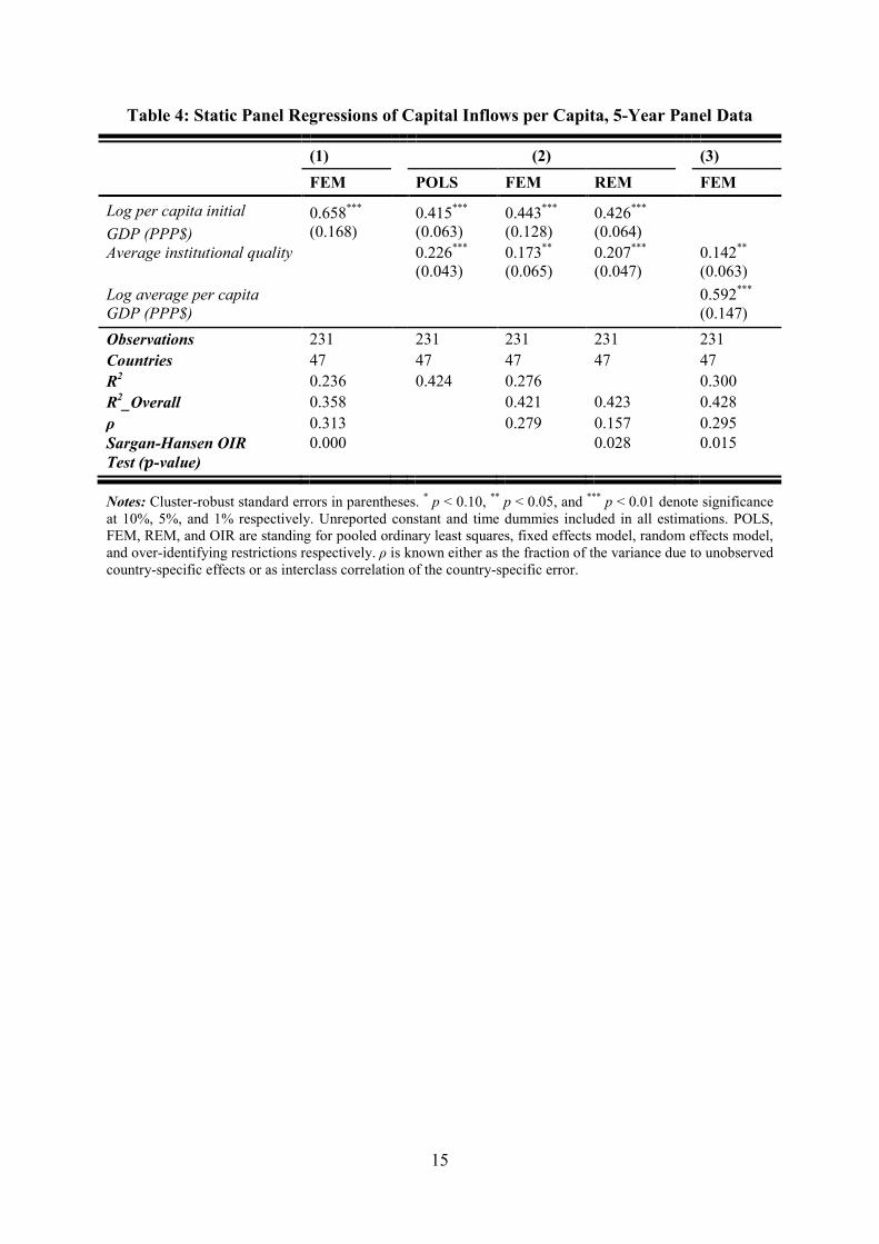
Table 4 reports the basic static panel data regression results. Since the Sargan-Hansen OIR

test implies that REM is inconsistent only FEM estimates are given under the first

specification. Controlling for time invariant country-specific heterogeneity, fixed effects

estimation shows that capital moves to relatively wealthier economies; allowing for within-

group variation the Lucas paradox exists. Under models (2) and (3), fixed effects (likewise

POLS and REM) estimates for initial income and institutions are positive and highly

significant (at 1% and 5% respectively). Hence, the quality of institutions cannot explain the

paradox for developing countries in the short-run when time series variations are also taken

into account.

[Table 4]

Table 5 includes additional covariates. The fraction of the composite error variance due to

unobservable country-specific fixed effects (ρ) is very high leading the Sargan-Hansen OIR

7 Arellano (1993) and Wooldridge (2002, pp. 290-91) propose more technical approaches for this test.

8

test to always reject the asymptotic appropriateness of the REM. Following the practices in

some empirical papers testing the postulations of gravity models of trade I include both fixed

distance and time varying remoteness variables simultaneously under the remaining

regressions.8 In line with the models under (2) and (3) in the previous table, all of the Table 5

estimations demonstrate that within developing countries the paradox prevails, not only

across countries but also over time no matter how significant are the additional explanatory

variables.

[Table 5]

4.2 Sensitivity Analyses

Through a number of alternative specifications with different proxy variables I document

that all of the static panel within-group fixed effects, pooled OLS and random effects GLS

techniques consistently deliver similar estimates that are implicationally robust. 9 Regressions

reported in Table 6 include some aspects of the host country economic fundamentals

alongside initial GDP per capita and institutional quality. Validated by the pertinent OIR

tests, REM under (1) and (3) and FEM under (2) show that the paradox is still left

unexplained despite controlling for corporate tax, trade openness and deposit money bank

assets as well as institutions.

[Table 6]

From Table 7 it seems as if institutional quality accounts for the capital flows and the

Lucas paradox under FEM (2) but when I replace initial income with initial GCF in FEM (2)

of Table 5 the quality of institutions variable is not significant whilst initial capital stock is.

Albeit not equivalently consistent, POLS and REM yield the results (unreported) that they

both are significant under (2). All the other regressions maintain the finding that the paradox

unresolved for developing countries.

[Table 7]

Table 8 reports the results considering proxy variables for sovereign risk (average risk

level, OECD taxonomy), international knowledge spillovers (average international voice

8 See Brun et al. (2005), Guttmann and Richards (2006), and Coe et al. (2007) for empirical; and Deardorff (1998), and Anderson and van Wincoop (2003) for theoretical treatments.

9 Outliers detecting added variable plots (available upon request) indicate that Chile and Panama may have influential observations. My key results are left unaltered, however, when I drop either of them in turn or suppress both at once.

9

traffic) and asymmetric information (average foreign bank asset share). The relevant

estimations throughout the table reassure that including country risk, global phone traffic and

foreign bank penetration have no influence at all on the prevalence of the paradox.

[Table 8]

4.3 Static Panel Instrumental Variable Regressions

It might be the case that there is a feedback from capital inflows per capita (the dependent

variable) to the quality of institutions (one of the key regressors). More generally, there may

be an omitted variable that influences both of these. Thus, one cannot discount the possibility

of endogeneity of the institutional quality variable. To address this I adopt a panel

instrumental variables approach. Table 9 below gives the linear cross section-time series

instrumental variable (IV) regressions in addition to the first stage and primary panel data

estimations throughout Panels A, B and C. Under (1) and (2) institutional quality is

instrumented solely by the time invariant variable of log European settler mortality. Since this

implicit instrument does not change over time FEM estimators do not work properly so that I

am unable to report any within-group estimate. Considering all the other two-stage least

squares (2SLS) for POLS and generalized two-stage least squares (G2SLS) for REM results,

Hausman regressor endogeneity tests suggest that the corresponding models in Panels A and

C are asymptotically equivalent. Excessively larger standard errors in Panel A reinforces this

also that institutional quality is actually exogenous to the conventional static panel

specifications. As a last remark, the second part of Panel C shows that the Lucas paradox

persists even within the adjusted sample.

[Table 9]

To see whether the colonizer mortality (main instrument) is excludable in the second stage

and to test the validity of all the instruments I run further two-way error components IV

regressions and provide the results under specification (3) in Table 9. Here I additionally

employ fixed but observable variables of British legal origin and English language as implicit

instruments besides explicitly controlling for European settler mortality as another instrument

for the quality of institutions. Albeit Sargan test for over-identifying restrictions validates

those instruments, the Hausman regressor endogeneity test and very high standard errors

(Panel A) imply that institutional quality is independent from the idiosyncratic errors (i.e.

exogenous).

10

5. Dynamic Panel Estimations

As noted above, to capture dynamic relationships consistently I employ two-way error

components models of generalized method of moments (GMM). I report results from the

Blundell and Bond (1998) system GMM estimator as the main variables of interest are quite

persistent over time.10

5.1 Fundamental Results

Through six dynamic model settings Table 10 provides the system GMM results testing

the presence of the Lucas paradox and looking whether it disappears when allowing for

institutional quality and other control variables. Specification fitted under (1) once again

shows that the paradox indeed exists within this autoregressive dynamic panel framework.

Inclusion of the quality of institutions leaves the paradox unresolved as in the static panel

cases. In parallel with these, estimations controlling for human capital, unilateral distance,

capital controls and remoteness in addition to initial income and institutions demonstrate that

the Lucas paradox persists when the autoregressivity in the dependent variable is allowed for.

Also there is positively significant (one period) state dependence under all specifications in

the table.

[Table 10]

5.2 Robustness Checks

Controlling for trade openness, level of financial sector development, total factor

productivity growth, initial capital stock per capita, malaria incidence and international

communication traffic in Table 11 do not alter the mainstay of the dynamics characterized

above. Coefficients on the lags of the dependent variable give a monotonic adjustment to a

shock that is over after two 5-year periods. The positive significance of the first lag

effectively narrows this decay to a 5-year period. This is consistent with my interpretation of

the estimates from the five-year panel data as the short-run parameters in that it takes five

years for an impact on the contemporaneous capital flows (i.e. ���) to die out, after which ��� reverts to its long-run level.11

[Table 11]

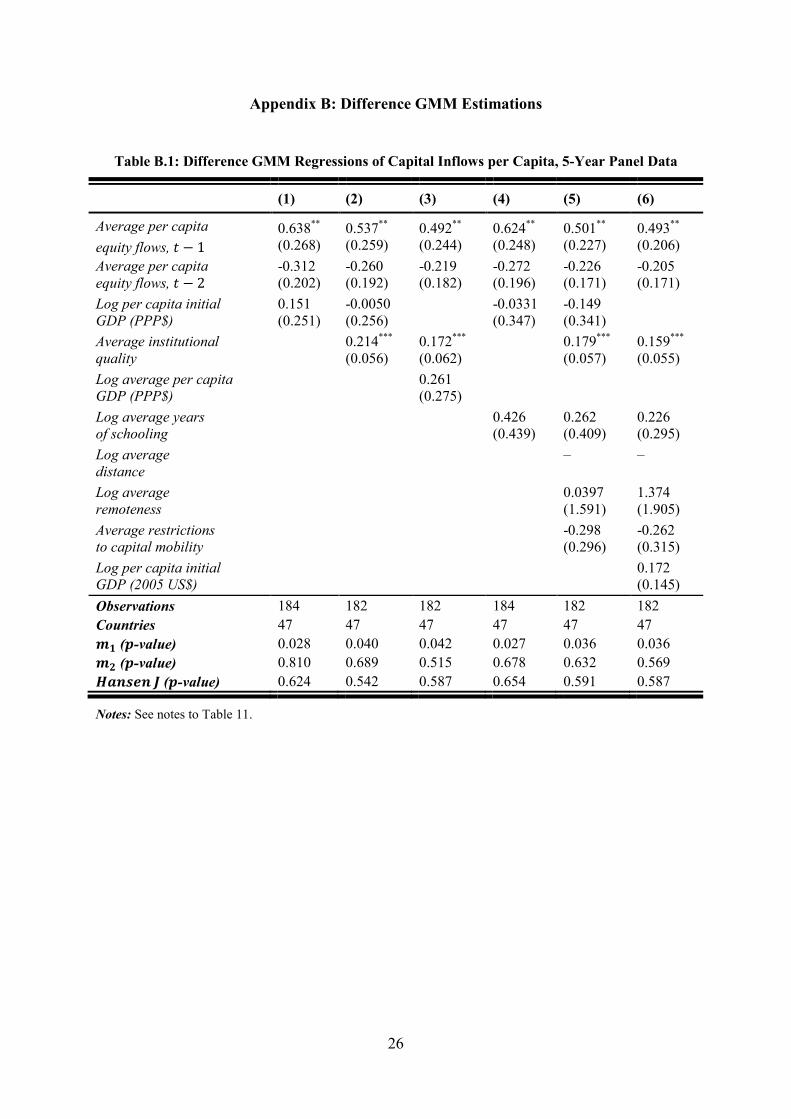
10 Arellano-Bond difference GMM results are demoted to the appendix.

11 Because � ≤ 2 for corporate tax, country risk and foreign bank penetration the dynamic models including them are unspecified. Hence, I am unable to report robustness checks for those extra explanatory variables.

11

6. Conclusion

This paper augments the analysis in Keskinsoy (2017) by implementing static (including

within-group fixed effects) and dynamic (system GMM) panel estimators. These estimators

are used to capture short-run dynamic relationships and to deal with any possible omitted

variables problem. For a panel of five-year moving averages over 1980-2006 and for 47

developing countries, the paper probes whether the wealth bias in international financial

flows (the Lucas paradox) is resolved in the short-run. It also tests if the short-run predictions

of Acemoglu and Zilibotti (1997) hold. I demonstrate that the persistence in the Lucas

paradox within developing countries is so entrenched that allowing for unobserved country-

specific effects, within-group (time series) variation and autoregressive dynamics do not

resolve the paradox.

The results are identical within and across static panel data methods. Within-group fixed

effects regressions imply (as equivalently consistent random effects GLS regressions do in

some cases) that the paradox remains in the short-run for developing economies. Although

institutional quality has positive impact on capital flows to these economies, it is unable to

resolve the wealth bias. Capturing the dynamics and controlling for endogeneity, Blundell-

Bond style system GMM estimations indicate that the existence and persistence of the Lucas

paradox is an intertemporal phenomenon within developing countries. They also show that

real capital flows per capita have positive, one five-year period state dependence or inertia.

This additionally justifies the short-run interpretation throughout the paper.

The persistence in the Lucas paradox and associated non-convergence in real incomes,

factor prices and returns could be attributed to a Linder-type home bias in international

finance. It may also be the case that excessive volatility in financial markets and related

behavioural anomalies in certain types of external funding breed the negative shocks that

cancel out the effects of positive shocks. This may eventually give rise to a permanent

diversion in the direction of funding.

12

Tables and Figures

Table 1: Standard Deviation Decompositions and Coefficients of Variation of the Data

Proportional Deviations Coef. of Variation

Variables Annual Sample 5-Year Sample Annual Sample

Between Within Between Within Between Within

Per capita equity flows 46.81 53.19 51.92 48.08 1.40 0.65

Per capita initial GDP 100 0 49.41 50.59 0.67 —

Institutional quality 43.84 56.16 46.42 53.58 0.11 0.10

Average years of schooling 64.55 35.45 64.55 35.45 0.45 0.23

Weighted-average remoteness 86.43 13.57 87.89 12.11 0.19 0.01

Capital mobility barriers 44.49 55.51 48.35 51.65 0.31 0.16

Corporate tax rate 70.39 29.61 79.90 20.10 0.18 0.02

Trade openness 66.29 33.71 69.66 30.34 0.49 0.12

Deposit money bank assets 58.32 41.68 59.12 40.88 0.56 0.21

TFP growth 26.26 73.74 38.26 61.74 -6.81 -4.38

Per capita initial GCF 100 0 55.84 44.16 1.04 —

Malaria contagion risk 100 0 100 0 0.87 —

Risk level, OECD 78.93 21.07 81.81 18.19 0.30 0.02

International voice traffic 73.46 26.54 75.37 24.63 1.85 1.11

Foreign bank asset share 77.77 22.23 84.62 15.38 0.93 0.12

Notes: Equity flows are the sum of international portfolio equity and direct investment inflows expressed in constant 2005 US dollars divided by the total population. Percentage proportions for standard deviations of each variable across countries, between, versus over time, within, under annually observed and five-year averaged samples. Cross country (time averaged data) and over time (country averaged data) coefficient of variations are calculated for annual sample only. GCF is gross capital formation.

13

Figure 1: Capital Inflows per Capita by Sub-periods, 1970-2006

Notes: See notes to Table1.

Table 2: Summary Statistics, Five-Year Panel Data

Variables Sample Mean Std. Dev. Min Max

Per capita equity flows 231 51.047 78.533 -147.875 482.952

Per capita initial GDP ($PPP) 231 3.439 2.303 0.406 11.647

Institutional quality 231 5.733 1.103 3.168 7.804

Average years of schooling 231 4.352 1.887 0.370 9.740

GDP- weighted average remoteness 231 8.913 1.617 5.840 12.501

Average capital mobility barriers 231 0.585 0.303 0.000 1.000

Corporate tax rate 68 30.118 5.542 15.000 42.220

Trade openness 231 64.961 35.735 12.146 207.290

Deposit money bank assets 212 0.355 0.251 0.040 1.526

TFP growth 180 -0.422 2.675 -8.390 5.166

Per capita initial GCF (2005 $US) 230 0.524 0.482 0.019 2.783

Malaria contagion risk as of 1994 141 0.418 0.398 0.000 1.000

Risk level, OECD 94 5.106 1.542 2.000 7.000

International voice traffic 160 27.011 42.203 0.066 289.080

Foreign bank asset share 77 0.224 0.202 0.006 0.900

Notes: See notes to Table 1.

0

1

2

3

4

5

6

7

8

Tota

l E

quit

y I

nfl

ow

s in

Th

ousa

nds

of

2005 U

SD

1970-74 1975-79 1980-84 1985-89 1990-94 1995-00 2001-06

Periods

14

Table 3: Pearson Product-Moment Correlation Coefficients, Five-Year Panel Data

Equity

Flows pc

Log pc

IGDP

Quality of

Institutions

Log

Schooling

Log

Distance

Barriers to

Cap. Mob.

L. pc IGDP

p-value

0.444 0.000

Institutions p-value

0.508 0.000

0.496 0.000

Log schooling p-value

0.367 0.000

0.707 0.000

0.424 0.000

Log distance

p-value

0.103 0.033

0.101 0.036

0.090 0.146

0.273 0.000

Restrictions

p-value

-0.307 0.000

-0.258 0.000

-0.385 0.000

-0.208 0.000

-0.172 0.000

Corporate tax p-value

-0.236 0.043

-0.082 0.487

-0.197 0.102

-0.069 0.565

0.033 0.782

0.099 0.400

Log openness p-value

0.359 0.000

0.287 0.000

0.261 0.000

0.180 0.001

-0.020 0.675

-0.329 0.000

L. Bank assets

p-value

0.373 0.000

0.527 0.000

0.339 0.000

0.378 0.000

-0.020 0.706

-0.265 0.000

TFP growth

p-value

0.107 0.125

-0.062 0.373

0.106 0.129

-0.003 0.968

0.057 0.410

-0.175 0.012

Log pc IGCF p-value

0.454 0.000

0.687 0.000

0.368 0.000

0.514 0.000

0.046 0.359

-0.187 0.000

Malaria p-value

-0.250 0.000

-0.539 0.000

-0.295 0.000

-0.461 0.000

0.029 0.563

0.018 0.728

Country risk

p-value

-0.237 0.010

-0.578 0.000

-0.553 0.000

-0.449 0.000

-0.113 0.229

0.090 0.336

Voice traffic

p-value

0.626 0.000

0.374 0.000

0.379 0.000

0.286 0.000

-0.120 0.081

-0.187 0.006

Foreign bank p-value

-0.218 0.043

-0.348 0.001

-0.067 0.544

-0.195 0.083

0.215 0.045

-0.121 0.266

Notes: Barriers-to-Capital and Restrictions are interchangeably used terms for the same variable of average restrictions to and controls on capital mobility imposed by a country. The abbreviations L, I, and pc refer to ‘logs’, ‘initial’ and ‘per capita’ respectively. Country observations change from pair to pair adjusting to data availability. See notes to Table 2.

15

Table 4: Static Panel Regressions of Capital Inflows per Capita, 5-Year Panel Data

(1) (2) (3)

FEM POLS FEM REM FEM

Log per capita initial

GDP (PPP$)

0.658*** (0.168)

0.415*** (0.063)

0.443*** (0.128)

0.426*** (0.064)

Average institutional quality

0.226*** (0.043)

0.173** (0.065)

0.207*** (0.047)

0.142** (0.063)

Log average per capita

GDP (PPP$)

0.592*** (0.147)

Observations 231 231 231 231 231

Countries 47 47 47 47 47

R2 0.236 0.424 0.276 0.300

R2_Overall 0.358 0.421 0.423 0.428

ρ 0.313 0.279 0.157 0.295

Sargan-Hansen OIR

Test (+-value)

0.000 0.028 0.015

Notes: Cluster-robust standard errors in parentheses. * p < 0.10, ** p < 0.05, and *** p < 0.01 denote significance at 10%, 5%, and 1% respectively. Unreported constant and time dummies included in all estimations. POLS, FEM, REM, and OIR are standing for pooled ordinary least squares, fixed effects model, random effects model, and over-identifying restrictions respectively. ρ is known either as the fraction of the variance due to unobserved country-specific effects or as interclass correlation of the country-specific error.

16

Table 5: Static Panel Regressions with Alternative Covariates, 5-Year Panel Data

(1) (2) (3)

FEM POLS FEM REM FEM

Log per capita initial

GDP (PPP$)

0.592** (0.240)

0.375*** (0.089)

0.531*** (0.194)

0.400*** (0.096)

Log average years of schooling

0.161 (0.310)

0.0478 (0.107)

-0.199 (0.309)

0.0357 (0.111)

0.573** (0.225)

Average institutional

quality

0.180*** (0.044)

0.0785 (0.082)

0.147*** (0.050)

0.124 (0.091)

Log average

distance

-3.332 (2.399)

–

-3.736* (2.040)

–

Log average remoteness

3.571 (2.489)

5.278*** (1.734)

3.975* (2.112)

5.977*** (2.032)

Average restrictions to capital mobility

-0.313 (0.233)

-0.398 (0.269)

-0.323 (0.205)

-0.368 (0.277)

Log per capita initial

GDP (2005 US$)

0.379** (0.178)

Observations 231 231 231 231 231

Countries 47 47 47 47 47

R2 0.237 0.451 0.318 0.309

R2_Overall 0.361 0.147 0.450 0.174

ρ 0.313 0.774 0.167 0.839

Sargan-Hansen OIR

Test (+-value)

0.000 0.000 0.000

Notes: The dash “–” signifies automatic drop of corresponding regressor because of collinearity or model algorithm. See notes to Table 4.

17

Table 6: Robustness Static Panel Regressions of Capital Inflows, 5-Year Panel Data

(1) (2) (3)

REM POLS FEM REM REM

Log per capita initial

GDP (PPP$)

0.712*** (0.126)

0.410*** (0.063)

0.475*** (0.155)

0.417*** (0.065)

0.457*** (0.073)

Average institutional quality

0.550*** (0.111)

0.212*** (0.042)

0.176** (0.067)

0.199*** (0.048)

0.229*** (0.050)

Average corporate

tax rate

-0.0190 (0.030)

Log average trade

openness

0.131 (0.102)

-0.104 (0.184)

0.111 (0.101)

Log average deposit money bank assets

0.0222 (0.081)

Observations 68 231 231 231 212

Countries 36 47 47 47 46

R2 0.431 0.277

R2_Overall 0.552 0.401 0.431 0.448

ρ 0.603 0.298 0.149 0.123

Sargan-Hansen OIR

Test (+-value)

0.169 0.004 0.179

Notes: The number of observations may change due to data availability. See notes to Table 5.

Table 7: Robustness Static Panel Regressions of Capital Inflows, 5-Year Panel Data

(1) (2) (3)

POLS FEM REM FEM REM

Log per capita initial

GDP (PPP$)

0.496*** (0.072)

0.495*** (0.139)

0.516*** (0.068)

0.617*** (0.117)

Average institutional quality

0.229*** (0.059)

0.0916 (0.094)

0.187*** (0.066)

0.251*** (0.075)

0.326*** (0.062)

Log average

TFP growth

0.0305* (0.018)

0.0377 (0.024)

0.0313* (0.019)

Log per capita initial GCF (2005 $US)

0.0291 (0.108)

Malaria contagion risk

0.134 (0.166)

Observations 180 180 180 230 141

Countries 39 39 39 47 47

R2 0.501 0.293 0.237

R2_Overall 0.485 0.499 0.330 0.480

ρ 0.348 0.153 0.356 0.297

Sargan-Hansen OIR

Test (+-value)

0.006 0.000 0.174

Notes: See notes to Table 6.

18

Table 8: Robustness Static Panel Regressions of Capital Inflows, 5-Year Panel Data

(1) (2) (3)

POLS FEM REM FEM REM

Log per capita initial

GDP (PPP$)

0.660*** (0.090)

0.421 (0.485)

0.648*** (0.089)

0.288* (0.166)

0.598*** (0.169)

Average institutional quality

0.503*** (0.078)

0.159 (0.193)

0.447*** (0.074)

0.186 (0.132)

0.306*** (0.086)

Average risk level,

OECD taxonomy

0.0108 (0.062)

-0.290 (0.244)

-0.0201 (0.066)

Average Int'l voice

traffic

0.0030 (0.002)

Average foreign bank asset share

-0.434 (0.476)

Observations 94 94 94 160 77

Countries 47 47 47 46 41

R2 0.555 0.125 0.273

R2_Overall 0.427 0.553 0.431 0.409

ρ 0.627 0.406 0.372 0.431

Sargan-Hansen OIR

Test (+-value)

0.440 0.011 0.116

Notes: See notes to Table 7.

19

Table 9: Static Panel IV Regressions of Capital Inflows per Capita, 5-Year Panel Data

(1) (2) (3)

POLS REM POLS REM POLS REM

Panel A: Instrumental Variable Estimations

Average institutional quality

1.009*** (0.352)

1.007 (0.620)

0.318 (0.342)

0.286 (0.361)

1.212* (0.734)

1.212 (1.556)

Log per capita initial GDP (PPP$)

0.355 (0.284)

0.370 (0.324)

Log European settler mortality

0.0427 (0.177)

0.0434 (0.376)

Hausman RE (+) 0.374 0.756 0.999 0.999 0.859 0.988

Sargan OIR (+) 0.812

Panel B: First Stage for Average Institutional Quality

Log European settler mortality

-0.210** (0.084)

-0.212* (0.128)

0.166** (0.082)

0.212* (0.114)

-0.221** (0.085)

-0.222* (0.133)

Log per capita initial

GDP (PPP$)

0.918*** (0.102)

1.023*** (0.123)

British legal origin -0.200 (0.175)

-0.199 (0.274)

English language 0.473 (0.408)

0.473 (0.639)

R2 0.137 0.137 0.397 0.396 0.146 0.146

Panel C: Primary POLS and REM Regressions

Average institutional

quality 0.392*** (0.045)

0.333*** (0.046)

0.230*** (0.050)

0.210*** (0.050)

0.371*** (0.045)

0.323*** (0.046)

Log per capita initial GDP (PPP$)

0.426*** (0.072)

0.434*** (0.086)

Log European settler mortality

-0.134** (0.052)

-0.145* (0.074)

Observations 194 194 194 194 194 194

Countries 39 39 39 39 39 39

Notes: In Panels A and C the response variable is average capital (foreign direct and portfolio equity) flows per capita whereas in B it is the composite index of institutional quality. Hausman regressor endogeneity (RE) test compares each model between Panels A and C whilst Sargan over-identifying restrictions (OIR) test assesses the

validity of model instruments. For both tests given are )-values. Standard errors are in parentheses. Consult also notes to Table 8.

20

Table 10: System GMM Regressions of Capital Inflows per Capita, 5-Year Panel Data

(1) (2) (3) (4) (5) (6)

Average per capita

equity flows, � − 1

0.606*** (0.123)

0.564*** (0.133)

0.536*** (0.138)

0.598*** (0.125)

0.531*** (0.150)

0.541*** (0.135)

Average per capita

equity flows, � − 2

-0.257 (0.196)

-0.215 (0.178)

-0.218 (0.177)

-0.252 (0.196)

-0.189 (0.160)

-0.227 (0.168)

Log per capita initial GDP (PPP$)

0.348*** (0.059)

0.190*** (0.048)

0.310*** (0.072)

0.161** (0.073)

Average institutional quality

0.185*** (0.035)

0.171*** (0.033)

0.157*** (0.033)

0.171*** (0.033)

Log average per capita

GDP (PPP$)

0.247*** (0.054)

Log average years of schooling

0.0779 (0.111)

0.0645 (0.096)

0.0926 (0.077)

Log average distance

-1.328 (1.457)

-2.175 (1.437)

Log average remoteness

1.292 (1.486)

2.161 (1.493)

Average restrictions

to capital mobility

-0.184 (0.249)

-0.175 (0.235)

Log per capita initial GDP (2005 US$)

0.153*** (0.050)

Observations 229 229 229 229 229 229

Countries 47 47 47 47 47 47

,- (+-value) 0.021 0.026 0.026 0.021 0.026 0.025

,. (+-value) 0.624 0.527 0.516 0.610 0.474 0.636

/012314 (+-value) 0.803 0.740 0.739 0.800 0.735 0.736

Notes: All specifications comprise finite-sample adjustment, two-step estimator optimization and collapsed

GMM-style instruments. Unreported constant and time dummies included in all estimations. 56 and 57 are the

Arellano-Bond tests for first order and second order autocorrelations in the residuals whilst 89:&;:< is the test of over-identifying restrictions for all the model instruments. Because sample size is not an entirely well-defined concept in system GMM which effectively runs on two samples (in levels and in first-differences) simultaneously, I report the size of the untransformed (level) sample. Windmeijer’s finite-sample corrected cluster-robust standard errors in parentheses. See notes to Table 9.

21

Table 11: Robustness System GMM Regressions of Capital Inflows, 5-Year Panel Data

(1) (2) (3) (4) (5) (6)

Average per capita

equity flows, � − 1

0.566*** (0.128)

0.548*** (0.134)

0.552*** (0.144)

0.599*** (0.121)

0.511*** (0.110)

0.539*** (0.124)

Average per capita

equity flows, � − 2

-0.205 (0.180)

-0.192 (0.178)

-0.0391 (0.252)

-0.249 (0.178)

-0.259 (0.295)

-0.355 (0.280)

Log per capita initial GDP (PPP$)

0.191*** (0.050)

0.247*** (0.050)

0.225** (0.086)

0.306** (0.115)

0.279*** (0.089)

Average institutional quality

0.182*** (0.035)

0.211*** (0.037)

0.156*** (0.044)

0.209*** (0.037)

0.260*** (0.055)

0.250*** (0.064)

Log average trade

openness

0.0149 (0.070)

Log average deposit money bank assets

-0.0441 (0.050)

Log average TFP growth

0.0175 (0.015)

Log per capita initial GCF (2005 $US)

0.0878** (0.036)

Malaria contagion

risk

-0.0686 (0.153)

Log average Int'l voice traffic

0.0029 (0.034)

Observations 229 212 178 228 141 160

Countries 47 46 39 47 47 46

,- (+-value) 0.026 0.034 0.057 0.026 0.043 0.047

,. (+-value) 0.504 0.372 0.482 0.674 0.257 0.442

/012314 (+-value) 0.744 0.750 0.626 0.778 0.584 0.743

Notes: See notes to Table 10.

22

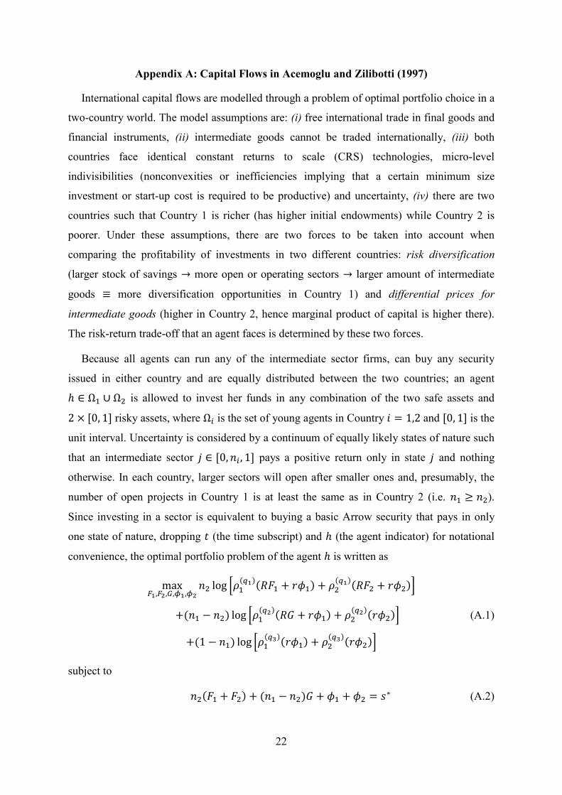
Appendix A: Capital Flows in Acemoglu and Zilibotti (1997)

International capital flows are modelled through a problem of optimal portfolio choice in a

two-country world. The model assumptions are: (i) free international trade in final goods and

financial instruments, (ii) intermediate goods cannot be traded internationally, (iii) both

countries face identical constant returns to scale (CRS) technologies, micro-level

indivisibilities (nonconvexities or inefficiencies implying that a certain minimum size

investment or start-up cost is required to be productive) and uncertainty, (iv) there are two

countries such that Country 1 is richer (has higher initial endowments) while Country 2 is

poorer. Under these assumptions, there are two forces to be taken into account when

comparing the profitability of investments in two different countries: risk diversification

(larger stock of savings → more open or operating sectors → larger amount of intermediate

goods ≡ more diversification opportunities in Country 1) and differential prices for

intermediate goods (higher in Country 2, hence marginal product of capital is higher there).

The risk-return trade-off that an agent faces is determined by these two forces.

Because all agents can run any of the intermediate sector firms, can buy any security

issued in either country and are equally distributed between the two countries; an agent

ℎ ∈ Ω6 ∪ Ω7 is allowed to invest her funds in any combination of the two safe assets and

2 × [0, 1] risky assets, where Ω� is the set of young agents in Country � = 1,2 and [0, 1] is the

unit interval. Uncertainty is considered by a continuum of equally likely states of nature such

that an intermediate sector E ∈ [0, :� , 1] pays a positive return only in state E and nothing

otherwise. In each country, larger sectors will open after smaller ones and, presumably, the

number of open projects in Country 1 is at least the same as in Country 2 (i.e. :6 ≥ :7).

Since investing in a sector is equivalent to buying a basic Arrow security that pays in only

one state of nature, dropping � (the time subscript) and ℎ (the agent indicator) for notational

convenience, the optimal portfolio problem of the agent ℎ is written as

maxIJ,IK,L,MJ,MK

:7 log QR6(SJ)(T�6 + UV6) + R7

(SJ)(T�7 + UV7)W

+(:6 − :7) log QR6(SK)(TX + UV6) + R7

(SK)(UV7)W (A.1)

+(1 − :6) log QR6(SY)(UV6) + R7

(SY)(UV7)W

subject to

:7(�6 + �7) + (:6 − :7)X + V6 + V7 = &∗ (A.2)

23

� is the amount of savings invested in risky asset and �[ ≥ \[ = max ]0, ^6#_ (E − `)a, where

\[ is the minimum investment to ensure productivity or positive return and the expression on

the right hand side (RHS) is its distribution function. There is no minimum investment

requirement for the sectors to be open if they satisfy E ≤ `. For the rest of the sectors, the

minimum investment requirement increases linearly in b(> 0), which captures the presence

of nonconvexities or indivisibilities that in turn shape the trade-off between insurance and

productivity or risk and return. V is the amount of savings invested in safe asset that has a

nonstochastic gross rate of return U(< T), where T is the rate of return on or payoff from the

investment in risky security. R refers interchangeably to the price of intermediate goods, the

aggregate rate of return on safe and risky financial investments and the marginal product of

capital. As intermediate goods are nontradable (Asmp. ii), R6[ ≠ R7[ . Given that :6 ≥ :7; if

the realized state of nature is E ∈ f6 ≡ [0, :7], a risky investment in both countries will have

a positive payoff. If E ∈ f7 ≡ [:7, :6], however, only risky investments in Country 1 will

have a positive payoff. Finally, if E ∈ fg ≡ [:6, 1], no risky projects will be successful. X is

the amount of investment in risky assets of Country 1 such that ∀ℎ and ∀E, Ei ∈ [:7, :6],

there exists �6[ = �6[j ≡ X. From the constraint, &∗ is the optimal savings of the agent.

The equilibrium solutions can be characterized from the first order conditions of the form

kKlJ(mJ)n

lJ(mJ)(nIJopMJ)olK

(mJ)(nIKopMK)= q:7 (A.3)

kKlK(mJ)n

lJ(mJ)(nIJopMJ)olK

(mJ)(nIKopMK)= q:7 (A.4)

(kJ#kK)lJ(mK)n

lJ(mK)(nLopMJ)olK

(mK)(pMK)= q(:6 − :7) (A.5)

kKlJ(mJ)p

lJ(mJ)(nIJopMJ)olK

(mJ)(nIKopMK)+ (kJ#kK)lJ

(mK)plJ(mK)(nLopMJ)olK

(mK)(pMK)+ (6#kJ)lJ

(mY)plJ(mY)(pMJ)olK

(mY)(pMK)= q (A.6)

kKlK(mJ)p

lJ(mJ)(nIJopMJ)olK

(mJ)(nIKopMK)+ (kJ#kK)lK

(mK)plJ(mK)(nLopMJ)olK

(mK)(pMK)+ (6#kJ)lK

(mY)plJ(mY)(pMJ)olK

(mY)(pMK)= q (A.7)

Given that :7∗ < 1, from (A.3) and (A.4) it follows that R6(SJ) = R7

(SJ), hence

T�6 + UV6 = T�7 + UV7 (A.8)

Using (A.3)-(A.5) to obtain the ratio

24

lJ(mJ)

lJ(mK) =

lJ(mJ)(nIJopMJ)olK

(mJ)(nIKopMK)lJ(mK)(nLopMJ)olK

(mK)(pMK) (A.9)

Given the production function = r�st6#s, factor prices u = (1 − �)r�s as the wage

earning or returns to labour and R = �r�s#6 as the marginal product of capital and optimal

savings &∗ = v6ov (1 − �)r�s in addition to :7∗ < 1, it follows from the law of decreasing

marginal returns to capital (DMRC) that there exists such a nontrivial relation (otherwise

contradiction arises); R6(SK) < R6

(SJ) = R7(SJ) ≡ R(SJ), hence X∗ > �6∗, which is also the case

due to higher minimum size requirement (Asmp. iii). Observing now that UV7 < T�7 +UV7 = T�6 + UV6, decreasing marginal productivity once again implies that R7

(SK) > R6(SJ) =

R7(SJ) ≡ R(SJ) > R6

(SK). Finally, subtracting (A.7) from (A.6)

(kJ#kK)lJ(mK)(nLopMJ)olK

(mK)(pMK)wR6

(SK) − R7(SK)x = (6#kJ)

lJ(mY)(pMJ)olK

(mY)(pMK)wR7

(SY) − R6(SY)x (A.10)

From R6(SK) < R7

(SK) it follows that R7(SY) < R6

(SY) which, in turn, implies by DMRC that

V7∗ > V6

∗ (A.11)

Since the optimal condition was T�6 + UV6 = T�7 + UV7, it finally proves

X∗ > �6∗ > �7∗ (A.12)

Equation (A.8) shows that the marginal product of capital or return on financial

investments is equal across countries (no matter whether they are rich or poor) for the

equilibrium subset of states f6∗ ≡ [0, :7∗], where the size of open sectors and the level of

associated investments are lower. The eleventh equation implies that the insurance role of the

safe asset is more important in Country 2 than in Country 1, so the risk free investments are

higher in the poorer country. Ultimately, the inequality in Equation (A.12) means that larger

scale and risky financial investments (X∗and �6∗)are higher in the richer country. Because the

return on risky assets is greater than the return on safe assets (i.e. T > U) and risky asset

purchases increase with the size and number of open sectors within the countries, risky

financial investments are more significant than safe ones. In other words, what is meant by

international capital flows are essentially those risky financial investments that are promoted

by return and diversification motives and take place across countries. Figure A.1 sketches the

resulting aggregate equilibrium capital flows in this two-country world. Both equilibrium

solutions at time � (recall that the time subscripts were dropped) and their aggregate images

25

in the figure (areas within the solid lines) demonstrate that more capital flows to the richer

country in the short-run.

Figure A.1: International Capital Flows in Acemoglu and Zilibotti (1997)

�6[y Country1

�7[y Country2

\[ \[

b b

X∗y

�6∗y

�7∗y

` :7∗ :6∗ 1 E, : ` :7∗ 1 E, :

This open economy model of optimal portfolio choice provides an alternative approach to

the direction and allocation of international capital, which is different than the approaches

previously considered. The model offers a time-dependent explanation and implies that the

neoclassical view, that the new financial investments will accrue to poorer economies, can

only be achieved in the long-run. In the short-run and under the governing assumptions of

micro-level nonconvexities (or indivisibilities) and uncertainty, it expects the foreign capital

to be destined to richer economies. Hence, there would be no paradox in such circumstances.

26

Appendix B: Difference GMM Estimations

Table B.1: Difference GMM Regressions of Capital Inflows per Capita, 5-Year Panel Data

(1) (2) (3) (4) (5) (6)

Average per capita

equity flows, � − 1

0.638** (0.268)

0.537** (0.259)

0.492** (0.244)

0.624** (0.248)

0.501** (0.227)

0.493** (0.206)

Average per capita

equity flows, � − 2

-0.312 (0.202)

-0.260 (0.192)

-0.219 (0.182)

-0.272 (0.196)

-0.226 (0.171)

-0.205 (0.171)

Log per capita initial

GDP (PPP$)

0.151 (0.251)

-0.0050 (0.256)

-0.0331 (0.347)

-0.149 (0.341)

Average institutional

quality

0.214*** (0.056)

0.172*** (0.062)

0.179*** (0.057)

0.159*** (0.055)

Log average per capita GDP (PPP$)

0.261 (0.275)

Log average years of schooling

0.426 (0.439)

0.262 (0.409)

0.226 (0.295)

Log average

distance

–

–

Log average

remoteness

0.0397 (1.591)

1.374 (1.905)

Average restrictions to capital mobility

-0.298 (0.296)

-0.262 (0.315)

Log per capita initial GDP (2005 US$)

0.172 (0.145)

Observations 184 182 182 184 182 182

Countries 47 47 47 47 47 47

,- (+-value) 0.028 0.040 0.042 0.027 0.036 0.036

,. (+-value) 0.810 0.689 0.515 0.678 0.632 0.569

/012314 (+-value) 0.624 0.542 0.587 0.654 0.591 0.587

Notes: See notes to Table 11.

27

Table B.2: Difference GMM Regressions of Capital Inflows per Capita, 5-Year Panel Data

(1) (2) (3) (4) (5) (6)

Average per capita

equity flows, � − 1

0.523* (0.262)

0.570** (0.256)

0.236 (0.639)

0.483*** (0.170)

0.476 (0.341)

0.327 (0.347)

Average per capita

equity flows, � − 2

-0.261 (0.193)

-0.224 (0.193)

-0.0827 (0.273)

-0.279 (0.168)

-0.348 (0.309)

-0.397 (0.293)

Log per capita initial

GDP (PPP$)

0.0615 (0.249)

0.110 (0.260)

0.314 (0.562)

0.0654 (0.544)

-0.0448 (0.680)

Average institutional

quality 0.224*** (0.059)

0.240*** (0.064)

0.166** (0.070)

0.214*** (0.055)

0.237*** (0.073)

0.226*** (0.077)

Log average trade openness

-0.270 (0.231)

Log average deposit money bank assets

-0.164 (0.135)

Log average

TFP growth

0.0182 (0.020)

Log per capita initial

GCF (2005 $US)

-0.0054 (0.096)

Malaria contagion risk

–

Log average Int'l voice traffic

0.165 (0.103)

Observations 182 166 139 181 139 112

Countries 47 46 39 47 47 45

,- (+-value) 0.042 0.040 0.325 0.017 0.120 0.146

,. (+-value) 0.757 0.441 0.668 0.703 0.561 0.904

/012314 (+-value) 0.512 0.604 0.561 0.613 0.516 0.549

Notes: See notes to Table B.1.

28

Appendix C: Data and Samples

Table C.1 Variable Descriptions and Sources

Variable Definition Source

Capital flows Sum of foreign direct and portfolio equity flows (also known as total equity flows) expressed in per capita 2005 $US.

World Development Indicators (WDI), World Bank.

Initial GDP Purchasing power parity (PPP) adjusted per capita GDP as of the model-corresponding initial year (mostly 1970), expressed in 2005 $US and in logs.

Heston et al. (2009), Penn Wold Table (PWT), Center for International Comparisons of Production, Income and Prices (CIC), University of Pennsylvania.

Institutional quality

A composite index constructed by adding up annual scores of twelve sub-indices (government stability, socioeconomic conditions, investment profile, internal conflict, external conflict, corruption, military in politics, religion in politics, law and order, ethnic tensions, democratic accountability, bureaucratic quality), rescaled by 10 and averaged over 1984-2006.

International Country Risk Guide (ICRG), Political Risk Services Group (PRS, 2007).

Years of schooling

Educational attainment of total population aged 25 and over in some levels (primary, secondary or tertiary) for some years, averaged over 1970-2000 and expressed in logs.

Barro and Lee (2001).

Distance Unilateral distance constructed as a GDP weighted average of the geodesic distances between capital city of a country and capital cities of all the other countries in the world, averaged over 1970-2006 and expressed in logs.

Centre d'Etudes Prospectives et d'Informations Internationales (CEPII) and World Development Indicators (WDI), World Bank.

Capital mobility restrictions

Taking values between 0 (if no restriction) and 1 (if there is restriction), it is the mean of four dummy variables (multiple exchange rate practices, restrictions on current account transactions, barriers on capital account dealings, and surrender and repatriation requirements for export proceeds), averaged over 1970-2005.

Annual Report on Exchange Arrangements and Exchange Restrictions (AREAER), IMF.

Corporate tax A percentage rate levied on the company profits in a country, averaged over 1999-2006.

Corporate and Indirect Tax Rate Survey (various years), KPMG.

Trade openness Exports plus imports expressed as a percentage of GDP and in logs, averaged over 1970-2006.

World Development Indicators (WDI), World Bank.

(continued on next page)

29

Table E.1 (continued)

Variable Definition Source

Deposit money bank assets

Ratio of deposit money bank assets to GDP, averaged over 1970-2006 and expressed in logs.

Financial Development and Structure Database, Beck et

al. (2000).

TFP growth The effect of technological change, efficiency improvements and immeasurable contribution of all inputs other than capital and labour which is estimated as the residual (i.e. Törnqvist index) by subtracting the sum of two-period average compensation share of capital and labour inputs weighted by their respective growth rates from the output growth rate. Usage of log level differences delivers the annual percentage TFP growth rates averaged over 1982-2006.

Total Economy Database, The Conference Board (2010).

Initial GCF Gross capital formation (GCF) per capita as of the model-corresponding initial year (mostly 1970) refers to outlays on additions to the fixed assets of the economy plus net changes in the level of inventories, expressed in 2005 $US and in logs.

World Development Indicators (WDI), World Bank.

Malaria The proportion of a country’s population at risk of falciparum malaria infection as of 1994.

Sachs (2003).

Country risk Countries are assessed in terms of credit risk and classified into eight numerical categories between 0 (lowest credit risk) and 7 (highest credit risk) using both quantitative and qualitative methods. Data is averaged over 1999-2006.

OECD, 2010.

International voice traffic

The sum of international incoming and outgoing telephone calls in minutes divided by the total population, averaged over 1970-2006 and expressed in logs.

World Development Indicators (WDI), World Bank.

Foreign bank asset share

Equals to the share of foreign bank assets in total banking sector assets, averaged over 1990-1997.

Financial Development and Structure Database, Beck et

al. (2000).

European settler mortality

The mortality rates of European settlers per 1,000 mean strength in the 19th century, expressed in logs.

Acemoglu et al. (2001).

British legal origin

A dummy variable indicating whether the origin of the current formal legal code of a country is British common law.

La Porta et al. (1997).

English language

Fraction of the population speaking English as mother tongue.

Hall and Jones (1999).

30

Table C.2: Country Samples

Baseline Sample IV Regressions Sample

Algeria Kenya Algeria Mexico

Argentina Malawi Argentina Nicaragua

Bangladesh Malaysia Bangladesh Niger

Bolivia Mali Bolivia Pakistan

Botswana Mexico Brazil Panama

Brazil Nicaragua Cameroon Papua New Guinea

Bulgaria Niger Chile Paraguay

Cameroon Pakistan China Peru

Chile Panama Colombia Senegal

China Papua New Guinea Costa Rica South Africa

Colombia Paraguay Dominican Republic Sri Lanka

Costa Rica Peru Ecuador Thailand

Dominican Republic Philippines Egypt Tunisia

Ecuador Senegal El Salvador Uruguay

Egypt South Africa Ghana Venezuela

El Salvador Sri Lanka Guatemala

Ghana Thailand Guyana

Guatemala Tunisia Honduras

Guyana Turkey India

Honduras Uruguay Indonesia

India Venezuela Jamaica

Indonesia Zambia Kenya

Jamaica Zimbabwe Malaysia

Jordan Mali

31

References

Acemoglu, D. & Zilibotti, F., 1997. Was Prometheus unbound by chance? Risk,

diversification, and growth. Journal of Political Economy, 105(4), pp. 709-751.

Acemoglu, D., Johnson, S. & Robinson, J.A., 2001. The colonial origins of comparative

development: An empirical investigation. American Economic Review, 91, pp. 1369-1401.

Ahn, S.C. & Schmidt, P., 1995. Efficient estimation of models for dynamic panel data.

Journal of Econometrics, 68, pp. 5-27.

Altonji, J.G. & Segal, L.M., 1996. Small-sample bias in GMM estimation of covariance

structures. Journal of Business and Economic Statistics, 14, pp. 353-366.

Anderson, J. & van Wincoop, E., 2003. Gravity with gravitas: A solution to the border

puzzle. The American Economic Review, 93, pp. 170-192.

Arellano, M., 1993. On the testing of correlated effects with panel data. Journal of

Econometrics, 59, pp. 87-97.

Arellano, M. & Bond, S., 1991. Some tests of specification for panel data: Monte Carlo

evidence and an application to employment equations. The Review of Economic Studies,

58, pp. 277-297.

Arellano, M. & Bover, O., 1995. Another look at the instrumental variables estimation of

error-component models. Journal of Econometrics, 68, pp. 29-51.

Baltagi, B.H., 2005. Econometric analysis of panel data, 3rd edition. West Sussex, England:

John Wiley & Sons Ltd.

Baltagi, B.H. & Griffin, J.M., 1984. Short and long run effects in pooled models.

International Economic Review, 25, pp. 631-645.

Barro, R.J. & Lee, J., 2001. International data on educational attainment: Updates and

implications. Oxford Economic Papers, 3, pp. 541-563.

Beck, T., Demirguc-Kunt, A. & Levine, R., 2000. A New Database on the Structure and

Development of the Financial Sector. The World Bank Economic Review, 14, pp. 597-605.

32

Blundell, R. & Bond, S., 2000. GMM estimation with persistent panel data: An application to

production functions. Econometric Reviews, 19(3), pp. 321-340.

Blundell, R. & Bond, S., 1998. Initial conditions and moment restrictions in dynamic panel

data models. Journal of Econometrics, 87, pp. 115-143.

Bowsher, C.G., 2002. On testing overidentifying restrictions in dynamic panel data models.

Economics Letters, 77, pp. 211-220.

Brun, J., Carrere, C., Guillaumont, P. & de Melo, J., 2005. Has distance died? Evidence from

a panel gravity model. World Bank Economic Review, 19, pp. 99-120.

Cameron, A.C. & Trivedi, P.K., 2005. Microeconometrics: Methods and Applications. New

York, NY: Cambridge University Press.

Centre d'Etudes Prospectives et d'Informations Internationales, 2009. Geodesic Distance

Database. Downloadable from http://www.cepii.fr/anglaisgraph/bdd/distances.htm.

Coe, D.T., Subramanian, A. & Tamirisa, N.T., 2007. The missing globalization puzzle:

Evidence of the declining importance of distance. IMF Staff Papers, 54, pp. 34-58.

Deardorff, A.V., 1998. Determinants of bilateral trade: Does gravity work in a neoclassical

world? In: Frankel, J. (Eds.), The Regionalization of the World Economy, The University

of Chicago Press, Chicago-IL.

Guttmann, S. & Richards, A., 2006. Trade openness: An Australian perspective. Australian

Economic Papers, 45, pp. 188-203.

Hall, R.E. & Jones, C., 1999. Why do some countries produce so much more output per

worker than others? The Quarterly Journal of Economics, 114, pp. 83-116.

Heston, A., Summers, R. & Aten, B., 2009. Penn World Table Version 6.3. Center for

International Comparisons of Production, Income and Prices; University of Pennsylvania.

Houthakker, H.S., 1965. New evidence on demand elasticities. Econometrica, 33, pp. 277-

288.

International Monetary Fund, 1970-2006. Annual Report on Exchange Arrangements and

Exchange Restrictions, various issues. Washington, DC: IMF.

33

Keskinsoy, B., 2017. Lucas paradox in the long-run. Unpublished manuscript.

KPMG International, 1999-2006. KPMG’s Corporate and Indirect Tax Rate Survey, various

issues. Downloaded from http://www.kpmg.com/GLOBAL/EN.

La Porta, R., Lopez-de-Silanes, F., Shleifer, A. & Vishny, R., 1997. Legal determinants of

external finance. Journal of Finance, 52, pp. 1131-1150.

Lucas, R.E., Jr., 1990. Why doesn't capital flow from rich to poor countries? The American

Economic Review, 80, pp. 92-96.

Lucas, R.E., Jr., 1988. On the mechanics of economic development. Journal of Monetary

Economics, 22, pp. 3-42.

Nerlove, M., 2002. Essays in Panel Data Econometrics. Cambridge University Press,

Cambridge-UK.

OECD, 2010. Country Risk Classifications of the Participants to the Arrangement on

Officially Supported Export Credits. Downloaded from http://www.oecd.org.

Pesaran, M.H. & Smith, R., 1995. Estimating long-run relationships from dynamic

heterogeneous panels. Journal of Econometrics, 68, pp. 79-113.

PRS Group, 2007. International Country Risk Guide Researchers Dataset. New York, NY:

The Political Risk Services Group.

Roodman, D., 2009. A note on the theme of too many instruments. Oxford Bulletin of

Economics and Statistics, 71, pp. 135-158.

Sachs, J.D., 2003. Institutions don’t rule: Direct effects of geography on per capita income.

NBER Working Paper 9490.

Sargan, J.D., 1958. The estimation of economic relationships using instrumental variables.

Econometrica, 26, pp. 393-415.

Schaffer, M.E. & Stillman, S., 2016. xtoverid: Stata module to calculate tests of

overidentifying restrictions after xtreg, xtivreg, xtivreg2 and xthtaylor. Available on

http://econpapers.repec.org/software/bocbocode/s456779.htm.

34

Sinn, S., 1992. Saving-investment correlations and capital mobility: On the evidence from

annual data. The Economic Journal, 102(414), pp. 1162-1170.

Tauchen, G., 1986. Statistical properties of generalized method-of-moments estimators of

structural parameters obtained from financial market data. Journal of Business and

Economic Statistics, 4, pp. 397-416.

The Conference Board, 2010. Total Economy Database. Downloaded from

http://www.conference-board.org/economics/database.cfm.

Windmeijer, F., 2005. A finite sample correction for the variance of linear efficient two-step

GMM estimators. Journal of Econometrics, 126, pp. 25-51.

Wooldridge, J.M., 2002. Econometric Analysis of Cross Section and Panel Data. Cambridge,

MA: The MIT Press.

Ziliak, J.P., 1997. Efficient estimation with panel data when instruments are predetermined:

An empirical comparison of moment-condition estimators. Journal of Business and

Economic Statistics, 15, pp. 419-431.