Macroscale water fluxes

3. Effects of land processes on variability of monthly

river discharge

P. C. D. MillyU. S. Geological Survey and Geophysical Fluid Dynamics Laboratory, NOAA, Princeton, New Jersey, USA

R. T. WetheraldGeophysical Fluid Dynamics Laboratory, NOAA, Princeton, New Jersey, USA

Received 9 July 2001; revised 15 April 2002; accepted 15 April 2002; published 15 November 2002.

[1] A salient characteristic of river discharge is its temporal variability. The time series offlow at a point on a river can be viewed as the superposition of a smooth seasonal cycle andan irregular, random variation. Viewing the random component in the spectral domainfacilitates both its characterization and an interpretation of its major physical controls from aglobal perspective. The power spectral density functions ofmonthly flow anomalies ofmanylarge rivers worldwide are typified by a ‘‘red noise’’ process: the density is higher at lowfrequencies (e.g., <1 y�1) than at high frequencies, indicating disproportionate (relative touncorrelated ‘‘white noise’’) contribution of low frequencies to variability of monthly flow.For many high-latitude and arid-region rivers, however, the power is relatively evenlydistributed across the frequency spectrum. The power spectrum of monthly flow can beinterpreted as the product of the power spectrum of monthly basin total precipitation (whichis typically white or slightly red) and several filters that have physical significance. Thefilters are associated with (1) the conversion of total precipitation (sum of rainfall andsnowfall) to effective rainfall (liquid flux to the ground surface from above), (2) theconversion of effective rainfall to soil water excess (runoff), and (3) the conversion of soilwater excess to river discharge. Inferences about the roles of each filter can be made throughan analysis of observations, complemented by information from a global model of theocean-atmosphere-land system. The first filter causes a snowmelt-related amplification ofhigh-frequency variability in those basins that receive substantial snowfall. The second filtercauses a relatively constant reduction in variability across all frequencies and can bepredicted well by means of a semiempirical water balance relation. The third filter,associated with groundwater and surface water storage in the river basin, causes a strongreduction in high-frequency variability of many basins. The strength of this reduction can bequantified by an average residence time of water in storage, which is typically on theorder of 20–50 days. The residence time is demonstrably influenced by freezing conditionsin the basin, fractional cover of the basin by lakes, and runoff ratio (ratio of mean runoff tomean precipitation). Large lake areas enhance storage and can greatly increase totalresidence times (100 to several hundred days). Freezing conditions appear to causebypassing of subsurface storage, thus reducing residence times (0–30 days). Small runoffratios tend to be associated with arid regions, where the water table is deep, andconsequently, most of the runoff is produced by processes that bypass the saturated zone,leading to relatively small residence times for such basins (0–40 days). INDEXTERMS: 1818

Hydrology: Evapotranspiration; 1854 Hydrology: Precipitation (3354); 1860 Hydrology: Runoff and

streamflow; KEYWORDS: temporal variability, spectral analysis, snowmelt, storage, residence time

Citation: Milly, P. C. D., and R. T. Wetherald, Macroscale water fluxes, 3, Effects of land processes on variability of monthly river

discharge, Water Resour. Res., 38(11), 1235, doi:10.1029/2001WR000761, 2002.

1. Introduction

1.1. Motivation

[2] The expected value of discharge of a river variesthrough the year, following the seasonal cycles of such

climatic variables as precipitation, solar radiation, and airtemperature. Superimposed upon this variation are random(chaotic) fluctuations at all timescales, reflecting everythingfrom decadal changes in the state of the climate system tothe rapid passage of a convective storm cell. The relativestrengths of these random variations, in turn, vary from onebasin to another around the globe. Much of hydrology is

This paper is not subject to U.S. copyright.Published in 2002 by the American Geophysical Union.

17 - 1

WATER RESOURCES RESEARCH, VOL. 38, NO. 11, 1235, doi:10.1029/2001WR000761, 2002

concerned with description and prediction of this variability,which so frequently manifests itself in floods and droughts.At the same time, a quantitative grasp of natural variabilityis a prerequisite for rigorous assessment of the significanceof recent and future changes in river flow.[3] Many random process models have been applied in the

analysis of flow variability [Bras and Rodrıguez-Iturbe,1985]. Use of such models, for example, to generate artificialtime series for engineering design, has long been common-place. Perhaps because of the wide variety and sophisticationof such models and the site-specific and goal-specific natureof such applications, however, no comprehensive synthesis ofthe diverse results has been attempted, and our global- scaleunderstanding of river flow variability remains limited.[4] Furthermore, random process models and their fitted

parameters are rarely interpreted in terms of the physicalprocesses that produce river flow. Nevertheless, the forcingof flow variations by weather and climatic variations is self-evident. How are precipitation fluctuations modulated bythe various components of the land-surface hydrologicsystem? What are the climatic and physiographic controlson the relevant processes? How can these factors bemodeled quantitatively? These are some of the questionsthat motivate the present study.[5] This work is also motivated by the need to character-

ize river discharge in global models of the land-ocean-atmosphere system. Applications of such models to climatesimulation and associated hydrologic analysis generallyfocus on basins that can be resolved by the models (e.g.,greater than 10,000 km2 in area) at timescales characterizingvariability of discharge from basins of such sizes.

1.2. Objectives of These Papers

[6] This is the third in a series of three papers analyzingcontrols on water balances of large land areas. Part 1 [Millyand Dunne, 2002a] describes the development of the dataset upon which the subsequent papers are based, withspecial attention to assessment of errors in estimates ofprecipitation. In part 2 [Milly and Dunne, 2002b], these dataare employed to analyze the control of interannual waterbalance variations by fluctuations in supplies of water(precipitation) and energy (surface net radiation). In thepresent paper (part 3), the data of part 1 and the results ofpart 2 are used to develop and quantify a conceptual pictureof land-process controls of monthly streamflow variability.[7] More specifically, the objectives of this paper are to

characterize the random component of temporal variability ofmonthly discharge from river basins and to identify thedominant physical controls of that variability. The emphasishere on the monthly (as opposed to daily or shorter) timescaleis driven by three factors: (1) the relative ease of access tomonthly flow and precipitation data on a global scale, (2) therelatively high attenuation of flow anomalies for medium tolarge basins at frequencies higher than those associated withthe monthly timescale, and (3) the desire to avoid a detailedanalysis of the surface drainage network that is needed tointerpret such higher-frequency (e.g., daily) flows.

2. Data

2.1. Observational Data

[8] We use the river-basin data set of part 1. The data setincludes continuous, long-term (median record length 54

years) monthly time series of precipitation and discharge for175 large (median area 51,000 km2) basins worldwide. Thebasin mean precipitation was estimated by interpolation ofpoint gauge values. Part 1 also quantified the uncertainty intheir estimates of basin mean precipitation. In the notationof part 1, statistical behavior of relative errors in the long-term annual mean were summarized by a parameter ya,

ya ¼ E e2a� �� �1=2

= pah i ð1Þ

in which E{} represents the expected value of a randomprocess, pa denotes long-term-mean annual total precipita-tion amount, circumflex denotes a gauge-based estimate,angle brackets denote areal average over a river basin, andea is the error in the estimate of long-term basin meanannual precipitation, h pai. Components of ea consideredinclude expected spatial-sampling errors in the absence oforographic effects, spatial-sampling errors associated withorographic effects, and errors in adjustments for gauge bias.In part 1, standard correlation-based methods were alsoapplied to develop estimates of the standard errors ofanomalies from the mean during any particular month oryear. As a summary measure of the anomaly errors, part 1introduced the parameter yn,

yn ¼ s2n=Var Pnh ið Þ; ð2Þ

in which sn2 is the variance of the error in the estimate of the

basin mean anomaly for year n, an overbar denotes anaverage over the period of record, and Var(hPni) is thevariance of the basin mean annual precipitation. Becauseboth the precipitation and the error of estimation of itsanomaly are nearly uncorrelated in time at the monthlylevel, the index yn is also approximately equal to the time-average ratio of variance of the error of monthly precipita-tion anomalies to the variance of monthly precipitation.[9] In this analysis, we focus on temporal variability

much more than on mean values. Accordingly, we are moreconcerned with minimizing yn than with controlling system-atic errors. A small value of yn implies that anomalyestimation errors are small compared to the variance ofthe anomalies themselves. For the analyses presented here,we use only a subset of the 175 basins for which yn is lessthan 0.25; this value is chosen as the smallest value that willstill leave a reasonable number of basins in the tropics andhigh latitudes. Additionally, we accept only those basins forwhich the characteristic relative error in long-term basinmean annual precipitation (ya) is less than 0.5. This value ischosen to remove only the most seriously biased cases,because bias will affect our assessment only indirectly. Theconstraint on yn reduced the data set to 134 basins, and theconstraint on ya reduced it further to 124. Of the 124 basins,19 are within 30� of the Equator, and 18 are poleward of55�N.

2.2. Air Temperature

[10] Station records of air temperature were obtainedfrom Global Historical Climatology Network (GHCN)version 2, produced jointly by the National Climatic DataCenter and the Carbon Dioxide Information Analysis Cen-ter. The data are expressed as monthly mean values fromabout 7000 stations worldwide. GHCN temperature data

17 - 2 MILLY AND WETHERALD: LAND PROCESSES AND MONTHLY RIVER DISCHARGE

have been subjected to an extensive set of quality-controlprocedures [Peterson et al., 1998]. The station records wereused to estimate long-term annual-mean basin mean temper-ature, following exactly the procedures described in part 1for precipitation.

2.3. Climate-Model Outputs

[11] We complemented our observational data with out-puts of unobservable variables from a global model of theland-atmosphere-ocean system. The model is the medium-resolution (3.75� longitude by 2.25� latitude land grid)climate model used by Knutson et al. [1999], and theexperiment is their 1000-year control run, which representsa steady state climate approximating that of the present-day.The land component of the model [Manabe, 1969] trackswater storage in a snowpack reservoir and a root zonereservoir. The root zone reservoir receives water from rain-fall and snowmelt and loses water by evaporation andrunoff; runoff occurs when necessary to prevent root zonestorage from exceeding the root zone soil water capacity,which is a parameter of the model. For this analysis, weused monthly-mean model outputs of rainfall, snowfall,snowmelt, and runoff. Outputs on the model grid wereaveraged over basin areas by use of the basin masksdescribed in part 1.

3. Theoretical Framework

3.1. Power Spectral Density and Gain Functions

[12] The temporal variability of any variable x(t) (such asriver discharge) can be characterized in the frequencydomain by use of the power spectral density function(power spectrum), which is defined as the Fourier transformof the autocorrelation function of x(t),

�xx wð Þ ¼Z1

�1

fxx tð Þexp �jwtð Þdt; ð3Þ

in which fxx(t) is the autocorrelation function,

fxx tð Þ ¼ E x t0ð Þx t0 � tð Þ½ ; ð4Þ

where E[ ] is the expectation operator and t 0 is any time. Theintegral of�xx(w) over all frequencies w yields the variance ofthe process x(t), and the function�xx(w) expresses the relativecontribution of variability at any frequency w to the totalvariance. For time averages xt over some period t, thevariance of xt is equal to the integral of �xx(w) from 0 to thefrequency associated with t,

s2t xð Þ ¼Z2p=t

0

�xx wð Þdw: ð5Þ

Herein we use the notation sm2(x) and sa

2(x) to denotevariances of monthly and annual values of a variable x,respectively.[13] The power spectrum can also be related to the

Fourier transform of x(t),

�xx wð Þ ¼ 2p X wð Þj j2; ð6Þ

in which X(w) is the Fourier transform of x(t). We consider alinear input-output relation of the form

o tð Þ ¼Z t

�1

i tð Þhio t � tð Þdt; ð7Þ

in which i(t) is the input, o(t) is the output, and hio(t) is theimpulse response function that describes the output thatwould result from a unit impulse input at time 0.Application of the Fourier transform yields the simplerelation

O wð Þ ¼ 2pHio wð ÞI wð Þ; ð8Þ

in which upper-case letters denote transforms. The function2p|Hio(w)| controls the amplification or attenuation of asignal of a given frequency in the conversion of an input toan output by the response function hio(t). Combination of(6) and (8) yields

�oo wð Þ ¼ Gio wð Þ�ii wð Þ; ð9Þ

in which we have introduced the gain function, Gio(w),defined by

Gio wð Þ ¼ 4p2 Hio wð Þj j2: ð10Þ

3.2. Decomposition of the Discharge Power Spectrum

[14] In this paper, we view river discharge as the finaloutput of a series of linear processes having the form (7).This may seem to be an extreme point of view, given theoften emphasized nonlinearity of hydrologic processes.However, linear theory is being applied here only toanomalies, or departures from the long-term mean seasonalwater balance, and is not being used to predict that balanceitself. We simply assume that anomalies are sufficientlysmall to be approximated by linear relations. One factorcontributing to the viability of this linearization is the factthat spatial and temporal averaging of local, heterogeneous,nonlinear processes can produce nearly linear processes atlarger scales. Ultimately, the internal consistency and phys-ical plausibility of the results obtained here must be con-sidered in evaluating the usefulness of this assumption.[15] The following variables are assumed to be related

linearly by sequential relations of the form (7): precipitation(rainfall plus snowfall) rate p(t), effective rainfall (liquidprecipitation plus snowmelt) rate l(t), runoff rate q(t), andbasin discharge rate y(t). The first three variables are basinmean values of point fluxes. In basins without snow, p(t) andl(t) are identical; in snow-affected basins, the transformationof p(t) to l(t) describes, in an average way, the temporarystorage of snow as snowpack. Runoff here refers to soilwater excess, which may manifest itself as downward orlateral drainage of the root zone or as surface runoffassociated with saturation of the soil surface. The conversionof runoff to discharge is controlled by basin storage, whichincludes storage as groundwater (below the root zone) andsurface water (streams, swamps, lakes, etc.). For this study,these reservoirs are lumped together, because observationaldata for their separation are not generally available. We

MILLY AND WETHERALD: LAND PROCESSES AND MONTHLY RIVER DISCHARGE 17 - 3

acknowledge our neglect of the effects of a plant canopy; acanopy may affect the net partitioning of precipitation intorunoff and evaporation, but is not expected to store appreci-able amounts of water at the monthly timescale. Our modelcontains no representation of the infiltration-excess mecha-nism of runoff production.[16] Application of the linear-response model to this

series of variables implies that the power spectrum ofdischarge is the product of the power spectrum of precip-itation and a series of terms describing frequency-dependentfiltering of the precipitation signal through the snowpack,root zone, and basin store,

�yy wð Þ ¼ �pp wð ÞGpl wð ÞGlq wð ÞGqy wð Þ; ð11Þ

In order to inject some of our understanding of low-frequency control of discharge into the analysis, it is helpfulto recast (11) as

�yy wð Þ ¼ �pp wð ÞGpy 0ð Þ Gpl wð ÞGpl 0ð Þ

� �Glq wð ÞGlq 0ð Þ

� �Gqy wð ÞGqy 0ð Þ

� �; ð12Þ

in which

Gpy 0ð Þ � Gpl 0ð ÞGlq 0ð ÞGqy 0ð Þ: ð13Þ

Our introduction here of zero-frequency values is aconvenient artifice that anticipates our findings that thesefactors tend to be independent of frequency at sufficientlylow frequency. In practice, we can then estimate the zero-frequency term as an average value over frequencies lessthan some threshold value (e.g., 1 y�1).[17] Equation (12) provides the theoretical framework for

this paper, whose objective is to explore the contribution ofthe five factors on the right side of the equation to thevariability of discharge. We examine each quantity in turn,using observational data to the extent possible, but com-plementing the data, where necessary, with informationderived from numerical modeling. We begin the analysiswith a description of the prominent features of �pp(w) and�yy(w), which describe the frequency dependence of varia-tions in precipitation and discharge anomalies, based solelyon observational data. We then show how the results of part2 yield an accurate, observationally based predictor ofGpy(0), which characterizes sensitivity of long-term meandischarge to long-term mean precipitation. The factor con-taining Gpl(w), which quantifies the role of snow storageand snowmelt in the conversion of precipitation variabilityto variability of effective rainfall, is estimated from numer-ical simulations of the snowmelt process in the frameworkof a climate model. The factor containing Glq(w), which

characterizes the role of soil water in converting effectiverainfall variability to that of runoff, is also viewed from amodeling perspective. Finally, the term involving Gqy(w),which represents the effect of basin storage on conversionof runoff variability to discharge variability, is evaluated asa residual, given estimates of the other quantities in (12).The result is used to parameterize a simple linear basinstorage model, and some physical controls on the modelresidence time are identified.[18] The combined use of observational and model-gen-

erated data is less realistic than exclusive use of observa-tional data. This is an unavoidable feature of the analyticapproach that we have chosen. Any systematic errors thatmay be present in the gain functions derived from the modelwould translate to corresponding errors in the inferred gainfunction describing basin storage. As we shall see, however,the factors evaluated by use of the model generally appearto contribute relatively little to discharge variability. Fur-thermore, only the shapes of these functions are derivedfrom the model; their absolute levels are set on the basis ofobservational and theoretical considerations.

4. Analysis

4.1. Representative Basins

[19] Given the large number of basins in the study, wecannot display the various power spectral density functionsfor all basins. For this reason, we instead devote manyfigures to the display of various integral measures of thespectral characteristics. Such summary measures, however,hide much of the interesting detail. Accordingly, we havechosen to display also various power spectra for a selectionof six representative basins. The basins were chosen torepresent ‘‘end-members’’ of behaviors that were notedacross the full population of basins. Characteristics of theselected representative basins are presented in Table 1. Thebasins of the Pechora and Gota alv Rivers are in the highlatitudes of northern Europe; the latter basin contains a largelake that strongly conditions the discharge characteristics.The Danube and Susquehanna River Basins are representa-tive of middle-latitude basins. The Nueces and MagdalenaRiver Basins are representative of hot/dry and hot/moistbasins, respectively, of the low latitudes.

4.2. Spectra of Observed Precipitation andObserved Discharge

[20] Representative power spectra of observed precipita-tion and discharge are presented in Figure 1. Most precip-itation spectra contain approximately equal power at allfrequencies, with no apparent spectral peaks associated withsuch physical phenomena as ENSO. The most frequently

Table 1. Characteristics of Representative River Basins

River Gauge LocationLatitude of BasinCentroid, �N

Basin Area,km2

Basin AnnualPrecipitation, mm

Basin Annual MeanTemperature, �C

Pechora Ust’ Tsil’ma (Russia) 65 248,000 760 �3Gota alv Vanersborg (Sweden) 59 47,000 750 5Susquehanna Harrisburg (Pennsylvania, USA) 41 62,000 1,110 9Danube Orsova (Romania) 47 576,000 965 9Nueces Three Rivers (Texas, USA) 29 40,000 610 21Magdalena Puerto Berrıo (Colombia) 4 74,000 2,100 19

17 - 4 MILLY AND WETHERALD: LAND PROCESSES AND MONTHLY RIVER DISCHARGE

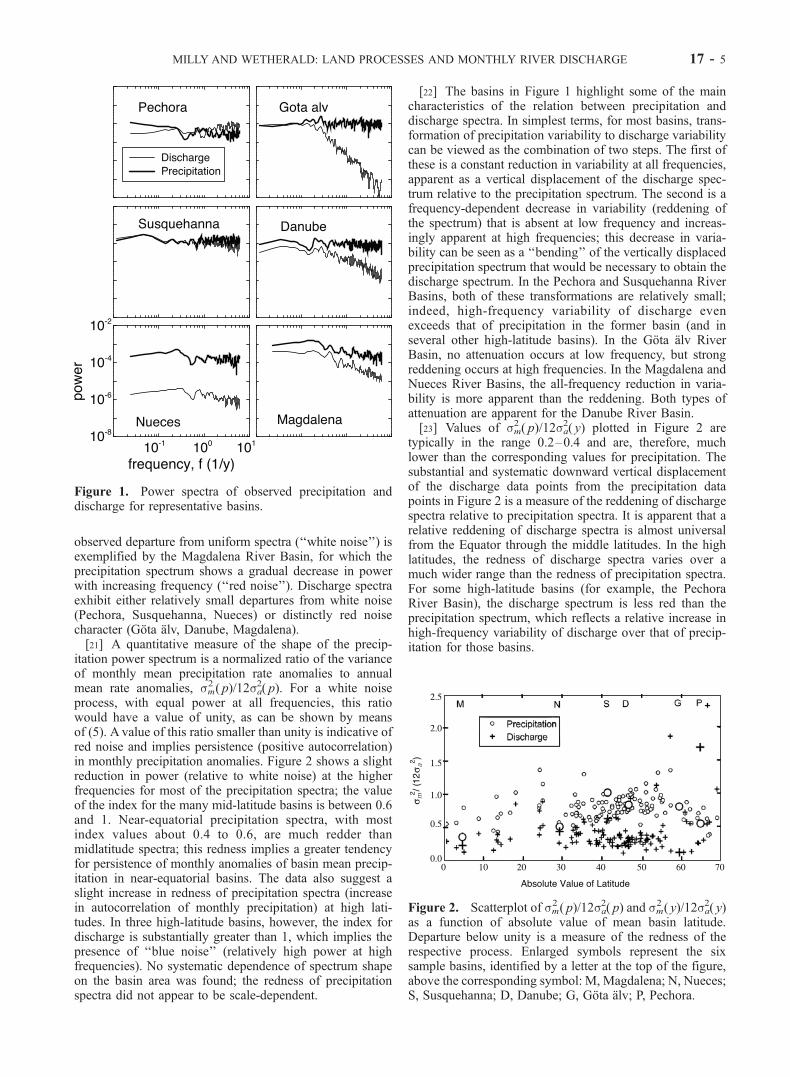
observed departure from uniform spectra (‘‘white noise’’) isexemplified by the Magdalena River Basin, for which theprecipitation spectrum shows a gradual decrease in powerwith increasing frequency (‘‘red noise’’). Discharge spectraexhibit either relatively small departures from white noise(Pechora, Susquehanna, Nueces) or distinctly red noisecharacter (Gota alv, Danube, Magdalena).[21] A quantitative measure of the shape of the precip-

itation power spectrum is a normalized ratio of the varianceof monthly mean precipitation rate anomalies to annualmean rate anomalies, sm

2 ( p)/12sa2( p). For a white noise

process, with equal power at all frequencies, this ratiowould have a value of unity, as can be shown by meansof (5). A value of this ratio smaller than unity is indicative ofred noise and implies persistence (positive autocorrelation)in monthly precipitation anomalies. Figure 2 shows a slightreduction in power (relative to white noise) at the higherfrequencies for most of the precipitation spectra; the valueof the index for the many mid-latitude basins is between 0.6and 1. Near-equatorial precipitation spectra, with mostindex values about 0.4 to 0.6, are much redder thanmidlatitude spectra; this redness implies a greater tendencyfor persistence of monthly anomalies of basin mean precip-itation in near-equatorial basins. The data also suggest aslight increase in redness of precipitation spectra (increasein autocorrelation of monthly precipitation) at high lati-tudes. In three high-latitude basins, however, the index fordischarge is substantially greater than 1, which implies thepresence of ‘‘blue noise’’ (relatively high power at highfrequencies). No systematic dependence of spectrum shapeon the basin area was found; the redness of precipitationspectra did not appear to be scale-dependent.

[22] The basins in Figure 1 highlight some of the maincharacteristics of the relation between precipitation anddischarge spectra. In simplest terms, for most basins, trans-formation of precipitation variability to discharge variabilitycan be viewed as the combination of two steps. The first ofthese is a constant reduction in variability at all frequencies,apparent as a vertical displacement of the discharge spec-trum relative to the precipitation spectrum. The second is afrequency-dependent decrease in variability (reddening ofthe spectrum) that is absent at low frequency and increas-ingly apparent at high frequencies; this decrease in varia-bility can be seen as a ‘‘bending’’ of the vertically displacedprecipitation spectrum that would be necessary to obtain thedischarge spectrum. In the Pechora and Susquehanna RiverBasins, both of these transformations are relatively small;indeed, high-frequency variability of discharge evenexceeds that of precipitation in the former basin (and inseveral other high-latitude basins). In the Gota alv RiverBasin, no attenuation occurs at low frequency, but strongreddening occurs at high frequencies. In the Magdalena andNueces River Basins, the all-frequency reduction in varia-bility is more apparent than the reddening. Both types ofattenuation are apparent for the Danube River Basin.[23] Values of sm

2 ( p)/12sa2( y) plotted in Figure 2 are

typically in the range 0.2–0.4 and are, therefore, muchlower than the corresponding values for precipitation. Thesubstantial and systematic downward vertical displacementof the discharge data points from the precipitation datapoints in Figure 2 is a measure of the reddening of dischargespectra relative to precipitation spectra. It is apparent that arelative reddening of discharge spectra is almost universalfrom the Equator through the middle latitudes. In the highlatitudes, the redness of discharge spectra varies over amuch wider range than the redness of precipitation spectra.For some high-latitude basins (for example, the PechoraRiver Basin), the discharge spectrum is less red than theprecipitation spectrum, which reflects a relative increase inhigh-frequency variability of discharge over that of precip-itation for those basins.

Figure 1. Power spectra of observed precipitation anddischarge for representative basins.

Figure 2. Scatterplot of sm2 ( p)/12sa

2( p) and sm2 ( y)/12sa

2( y)as a function of absolute value of mean basin latitude.Departure below unity is a measure of the redness of therespective process. Enlarged symbols represent the sixsample basins, identified by a letter at the top of the figure,above the corresponding symbol: M, Magdalena; N, Nueces;S, Susquehanna; D, Danube; G, Gota alv; P, Pechora.

MILLY AND WETHERALD: LAND PROCESSES AND MONTHLY RIVER DISCHARGE 17 - 5

[24] To facilitate an overview of the relative reddening ofthe discharge spectrum by surface processes, we show inFigure 3 the ratio of the discharge and precipitation rednessindices that were plotted in Figure 2. This is a measure ofthe extent to which high-frequency fluctuations are dampedmore than low-frequency fluctuations in the transformationfrom precipitation to discharge. From the Equator throughthe middle latitudes, discharge spectra in this data set areuniformly redder than precipitation spectra. The ratio ofdischarge redness to precipitation redness varies more athigh latitudes than elsewhere. Values of this ratio are evengreater than 1 for several basins, indicating that the dis-charge spectrum is less red than the precipitation spectrum;the Pechora River Basin has already been noted as anexample of such behavior. Figure 3 suggests that thisphenomenon may be correlated with the occurrence of anannual mean air temperature that is lower than the freezingpoint of water. We shall return to this observation later.

4.3. Low-Frequency Response

[25] A consistent feature of nearly all basins is near-parallelism (pure vertical offset without bending) of precip-itation and discharge spectra at low frequencies (i.e., typi-cally for timescales of 1 year and longer). This featureimplies frequency-independent transformation (preservationor reduction) of precipitation variability to discharge vari-ability at low frequencies. Within this low-frequencyregime, the difference between precipitation and dischargevariability (the vertical shift mentioned earlier) is highlyvariable across basins. In some basins (e.g., Susquehanna),discharge variability is nearly equal to precipitation varia-bility. In others (e.g., Nueces), discharge variability is one ormore orders of magnitude smaller than that of precipitation.A measure of the difference in low-frequency variabilitybetween discharge and precipitation is the ratio

Rwa

0

�yy wð Þdw

Rwa

0

�pp wð Þdw¼ s2a yð Þ

s2a pð Þ ; ð14Þ

in which wa is 2p/(1 year). A scatterplot of this quantityagainst latitude is presented as Figure 4, which shows a verywide range of values from near zero in some low- andmiddle-latitude basins to near one and even greater in somemiddle- and high-latitude basins. Also notable, however, isthe large variance of the index at most latitudes. In themiddle latitudes, the distribution of the index is bimodal,with a cluster of values near 0 (generally arid basins) and aspread of values above 0.5 (humid basins).[26] In part 2 it was shown that, to a good approximation,

observed low-frequency (annual and longer timescale) var-iations of discharge are mainly a response to low-frequencyprecipitation variations, with the sensitivity dependent onBudyko’s [1974] index of dryness, as originally suggested inthe context of numerical model experiments [Koster andSuarez, 1999]. Accordingly,

s2a yð Þs2a pð Þ ¼

dYn

dPn

� �2

; ð15Þ

where dYndPn

denotes the sensitivity of total discharge in wateryear n(Yn) to total precipitation in the same year (Pn). Toevaluate this sensitivity, we introduce the semiempiricalrelation

Y=P ¼ 1� f zð Þ; ð16Þ

in which z is the climatic index of dryness (ratio of long-term mean radiation, expressed as equivalent evaporativeflux, to long-term mean precipitation). Multiple functionalforms have been proposed for f(z). Although we found inpart 2 that the form of Budyko [1974] may be somewhatbiased, we chose to use it here; results obtained herein areinsensitive to the choice of f(z). Thus, we have [Budyko,1974]

Y=P

B¼ 1� z tanh z�1

1� cosh zþ sinh zð Þ

� �1=2; ð17Þ

Figure 3. Scatterplot of the ratio [sm2( y)/sa

2( y)]/[sm2( p)/

sa2( p)], which indicates the reltive damping of high

frequencies in the transformation of precipitation todischarge. Enlarged symbols represent the six samplebasins, identified by a letter at the top of the figure, abovethe corresponding symbol: M, Magdalena; N, Nueces; S,Susquehanna; D, Danube; G, Gota alv; P, Pechora.

Figure 4. Scatterplot of the ratio sa2( y)/sa

2( p) as a functionof absolute value of mean basin latitude. This ratioquantifies the attenuation of discharge variability relativeto that of precipittion at low frequencies. Enlarged symbolsrepresent the six sample basins, identified by a letter at thetop of the figure, above the corresponding symbol: M,Magdalena; N, Nueces; S, Susquehanna; D, Danube; G,Gota alv; P, Pechora.

17 - 6 MILLY AND WETHERALD: LAND PROCESSES AND MONTHLY RIVER DISCHARGE

where the subscript B indicates use of Budyko’s f(z). Withthe approximation that

dYn

dPn

¼ dY

dP; ð18Þ

we have also

dYn

dPn

� �B

¼ 1� 1

2z�1tanh z�1 1� e�z � ��1=2�

tanh z�1

1� e�z � ze�z þ z�1 sech z�1

21� e�z �

: ð19Þ

Together, (19) and (17) yielddYndPn

� �Bas a function of the ob-

served Y and P. The ability of (15), (19), and (17) to predictthe ratio in annual variances for the present data set is shownin Figure 5.[27] Under the approximation, supported by Figure 1 and

equivalent plots for the other basins, that precipitation anddischarge spectra are parallel for frequencies below wa, itfollows from (15) that

�yy wð Þ ¼ dYn

dPn

� �2

B

�pp wð Þ; w � wa: ð20Þ

This relation implies that

Gpy 0ð Þ ¼ dYn

dPn

� �2

B

: ð21Þ

[28] We have identified a convenient model for Gpy(0),but the relative contributions of snowpack, root zone, andbasin storage have not been identified. Such a decomposi-tion, of course, is not possible when only precipitation anddischarge data are used, but requires also accurate observa-tions of basin mean snowpack, root zone soil water, andgroundwater and surface water storage. Lacking such data,we can nevertheless make some judgments about the rolesof the various reservoirs. At very long timescales (i.e., in thelimit as w goes to 0), we expect storage rates in snowpack,soil, surface water, or groundwater to be insufficient to

affect variances of the respective outflows from thesereservoirs, so that outflows will be effectively in phase withinflows. (This expectation does not apply to glaciers, whoselong response times necessarily exclude them from ouranalysis.) If the rate of water flowing out of the snowpackand groundwater and (natural or man-made) surface waterreservoirs were essentially equal to the respective inflowrates (or, more precisely, if losses from these reservoirs wereindependent of inflow), it would follow that Gpl(w) andGqy(w) go to 1 for sufficiently small w. In contrast, wesuppose that low-frequency changes in inflow to the rootzone will result in changes both in outflow (runoff ) and inroot zone evaporation. Such assumptions are perhaps validin most environments, but inadequate in particular cases. Asan approximation, then, we expect that

Gpy 0ð Þ ¼ Glq 0ð Þ; ð22Þ

Gpl 0ð Þ ¼ Gqy 0ð Þ ¼ 1; ð23Þ

i.e., that the net low-frequency effect of all reservoirs in thebasin can be attributed to the soil water reservoir.

4.4. Snowpack Storage

[29] To estimate the contribution to discharge variabilitythat is associated with snow storage, the model-derived timeseries of precipitation and effective rainfall were analyzed.Sample spectra are plotted in Figure 6. The spectra show thatthe effect of snow is absent or negligible in the Magdalena,Nueces, Danube, and Susquehanna River Basins. These arebasins in which the change of snowpack mass is a small term

Figure 5. Scatterplot of the ratio of annual standarddeviations sa( y)/sa( p) against ðdYndPn

ÞB given by (19) and (17).Solid line is least squares fit (y = �0.012 + 0.998x; r =0.92), and dashed line is 1:1 line.

Figure 6. Power spectra of model output precipitation andeffective rainfall for representative basins.

MILLY AND WETHERALD: LAND PROCESSES AND MONTHLY RIVER DISCHARGE 17 - 7

in the monthly water balances of the model basins. Incontrast, the effect of snow storage is apparent in the twomost northern of the sample basins, the Pechora and the Gotaalv River Basins. Even in these basins, at frequenciescorresponding to periods greater than 1 year, the precipita-tion and effective-rainfall spectra are nearly identical. Thisresult supports our earlier assumption that dynamic, inter-annual storage of snow is negligible in non-glaciated basins.At higher frequencies, however, an increasing amplificationof variability of effective rainfall, relative to that of precip-itation, is apparent. This increase can be attributed to thecombination of two factors: (1) the short-term release, bymelting, of precipitation accumulated during the entiresnowfall season, and (2) the variability in timing of thisshort snowmelt period, which is associated with the varia-bility in energy availability from year to year. The height-ened variability of discharge at the shortest (monthly)timescale implies a negative lag-1 autocorrelation in theprocess at that timescale. Thus, for example, if snowmelt inApril is greater than normal, then snowpack and potential forsnowmelt will be less than normal in May. Our results areconsistent with those of Delworth and Manabe [1988],which were based on spectral analysis of precipitation outputfrom a similar model. They showed that the fraction ofvariability associated with high frequencies was greater foreffective rainfall than for precipitation at high latitudes.[30] Figure 7 is a plot against latitude of the ratio sm

2(l)/sm2 ( p), which expresses the contribution to discharge vari-

ability associated with snow storage and melting. Figure 7shows that the influence of snow on the spectra of effectiveprecipitation has a clear zonal dependence. It also shows,for a given latitude, that the magnitude of the effectincreases with the fraction of annual precipitation fallingas snow. This amplification of high-frequency variability inhigh latitudes, inferred from model output, is one factorhelping to explain the latitudinal variation in reddening ofdischarge spectra relative to precipitation spectra (Figure 3).

4.5. Soil Water Storage

[31] We first investigate the effect of soil water storage ondischarge variability by computing, for the model, the ratio

Glq(w)/Glq(0) (Figure 8). This quantity reflects the contribu-tion of root zone water balance dynamics to the relativereddening of the discharge power spectrum. In the middle-and low-latitude basins, a relatively small increase in rednesscan be detected. A simple measure of this tendency is theratio of sm

2 (q)/sa2(q) to sm

2 (l)/sa2(l). Perfectly parallel spectra

of effective rainfall and runoff would produce a value ofunity for this ratio. Relative reddening of runoff by soil waterstorage would produce values smaller than unity. The dis-tribution of this measure with latitude is shown in Figure 9.In the low and high latitudes, values of this index scatteraround 1, implying no systematic reddening of the signal bysoil moisture. In the middle latitudes, values average about0.8, implying a moderate damping of the higher frequencies.[32] In addition to their analysis of model precipitation

spectra, mentioned above, Delworth and Manabe [1988]also examined soil moisture spectra. They noted that nearlywhite precipitation input led to a red soil moisture spectrum,with strong damping of soil moisture fluctuations at themonthly timescale. Given the strong connection betweensoil moisture and runoff in the model, the relative absenceof redness in the runoff spectrum noted here may at firstseem surprising. In fact, soil moisture persistence in themodel is associated with seasons when the soil is usuallynot saturated, as a result of an excess of evaporative demandover precipitation. In the model, runoff occurs only inseasons when the soil reservoir is saturated, at which timesoil moisture has very short timescales. Thus, the runoff

Figure 7. Scatterplot of the ratio sm2(l)/sm

2 ( p) againstabsolute value of mean basin latitude. This ratio quantifiesthe amplification of effective rainfall variability relative tothat of precipitation. Enlarged symbols represent the sixsample basins, identified by a letter at the top of the figure,above the corresponding symbol: M, Magdalena; N, Nueces;S, Susquehanna; D, Danube; G, Gota alv; P, Pechora.

Figure 8. Model-derived estimates of Glq(w)/Glq(0) forrepresentative basins. This ratio reflects the frequencydependence of the transformation of infiltration variabilityto runoff variability. (Glq(0) was estimated as the averagevalue of Glq(w) over frequencies less than wa.)

17 - 8 MILLY AND WETHERALD: LAND PROCESSES AND MONTHLY RIVER DISCHARGE

parameterization is highly selective in sampling soil mois-ture variability. The net result is that soil moisture, at least inthis model parameterization, contributes very little to mod-ification of the shape of the power spectrum in the transitionfrom effective precipitation to runoff.

4.6. Effect of Groundwater and Surface WaterStorage on Discharge Variability

[33] We now use (12) to obtain an estimate of thecombined effect of groundwater and surface- water storageon the variability of discharge. We solve (12) for Gqy wð Þ

Gqy 0ð Þ, usingobservations to evaluate the precipitation and dischargespectra �pp(w) and �yy(w), and the model-derived estimatesof Gpl wð Þ

Gpl 0ð Þ andGlq wð ÞGlq 0ð Þ. To evaluate Gpy(0), we use (21), with (19),

(17), and the observations of long-term means of y and p.Note that the most important terms in (12) are thus eval-uated from the observations, and that the two model-evaluated factors are only weakly dependent on frequency.We expect this to lead to a fairly accurate estimate of Gqy wð Þ

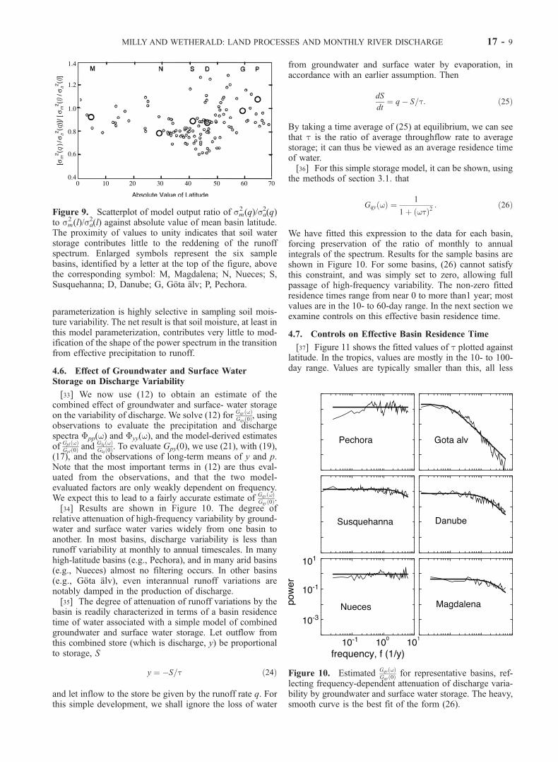
Gqy 0ð Þ.[34] Results are shown in Figure 10. The degree of

relative attenuation of high-frequency variability by ground-water and surface water varies widely from one basin toanother. In most basins, discharge variability is less thanrunoff variability at monthly to annual timescales. In manyhigh-latitude basins (e.g., Pechora), and in many arid basins(e.g., Nueces) almost no filtering occurs. In other basins(e.g., Gota alv), even interannual runoff variations arenotably damped in the production of discharge.[35] The degree of attenuation of runoff variations by the

basin is readily characterized in terms of a basin residencetime of water associated with a simple model of combinedgroundwater and surface water storage. Let outflow fromthis combined store (which is discharge, y) be proportionalto storage, S

y ¼ �S=t ð24Þ

and let inflow to the store be given by the runoff rate q. Forthis simple development, we shall ignore the loss of water

from groundwater and surface water by evaporation, inaccordance with an earlier assumption. Then

dS

dt¼ q� S=t: ð25Þ

By taking a time average of (25) at equilibrium, we can seethat t is the ratio of average throughflow rate to averagestorage; it can thus be viewed as an average residence timeof water.[36] For this simple storage model, it can be shown, using

the methods of section 3.1. that

Gqy wð Þ ¼ 1

1þ wtð Þ2: ð26Þ

We have fitted this expression to the data for each basin,forcing preservation of the ratio of monthly to annualintegrals of the spectrum. Results for the sample basins areshown in Figure 10. For some basins, (26) cannot satisfythis constraint, and was simply set to zero, allowing fullpassage of high-frequency variability. The non-zero fittedresidence times range from near 0 to more than1 year; mostvalues are in the 10- to 60-day range. In the next section weexamine controls on this effective basin residence time.

4.7. Controls on Effective Basin Residence Time

[37] Figure 11 shows the fitted values of t plotted againstlatitude. In the tropics, values are mostly in the 10- to 100-day range. Values are typically smaller than this, all less

Figure 9. Scatterplot of model output ratio of sm2 (q)/sa

2(q)to sm

2 (l)/sa2(l) against absolute value of mean basin latitude.

The proximity of values to unity indicates that soil waterstorage contributes little to the reddening of the runoffspectrum. Enlarged symbols represent the six samplebasins, identified by a letter at the top of the figure, abovethe corresponding symbol: M, Magdalena; N, Nueces; S,Susquehanna; D, Danube; G, Gota alv; P, Pechora.

Figure 10. Estimated Gqy wð ÞGqy 0ð Þ for representative basins, ref-

lecting frequency-dependent attenuation of discharge varia-bility by groundwater and surface water storage. The heavy,smooth curve is the best fit of the form (26).

MILLY AND WETHERALD: LAND PROCESSES AND MONTHLY RIVER DISCHARGE 17 - 9

than 30 days, in the subtropics. North of the subtropics, themedian value tends to increase with latitude through themiddle latitudes. In the high latitudes, the variance of t isvery large, with both the largest and smallest values foundin this zone.[38] The presence of substantial lake area in a basin appears

to explain many of the large values of t (Figure 11). Lakesgreatly increase the surface area of surface water in a basin,permitting relatively large changes in storage volume for agiven rise in discharge. By (24), this fact implies that thepresence of lakes tends to increase the value of t. Figure 11shows that seven of the nine largest values of t areassociated with basins in which lakes are estimated tocover more than 5% of the basin area; overall, only 16 ofthe 124 basins studied had such large fractional lake areas.The strong damping of variability in the Gota alv RiverBasin, one of our representative basins, can be understoodin terms of lake storage (Vanern Lake). Other lake-affectedbasins in our data set include the St. Lawrence (GreatLakes, t = 360 d), the Neva (Lake Ladoga, t = 320 d), theNelson (Lake Winnipeg, t = 150 d), and the White Nile(Lake Victoria, t = 160 d) River Basins.[39] We investigated further the two basins with t greater

than 100 days that did not have estimated fractional lakeareas greater than 5%. The investigation revealed that thesebasins were ‘‘exceptions that prove the rule.’’ In both basinsour estimates of fractional lake area were far too low as aresult of our use of a 1� basin map to represent small basins.In fact, these basins should have been grouped with theother lake-affected basins.[40] We found another strong control on high-latitude

variance of t to be the presence of freezing conditions.Figure 11 shows that the low values of t in high latitudesare associated with occurrence of annual mean temperaturesbelow the freezing point of water. Very approximately,regions of sub-freezing mean temperature tend to be regionsof continuous or discontinuous permafrost [Lunardini,1981]. Among our sample basins, the Pechora River Basin(annual mean temperature of �3 C, t = 1 d) is representa-

tive of the freezing-affected basins. Other such basinsinclude the Koyukuk River Basin in Alaska (�6 C, t = 0),and the Lena (�8 C, t = 0) and Yenisey (�4 C, t = 5 d)River Basins in Siberia.[41] We hypothesize that the widespread presence within

a basin of a frozen soil layer presents a barrier to exchangebetween surface and near-surface water (including theunfrozen ‘‘active layer’’ of the soil) and the deeper subsur-face. The loss of this major storage reservoir makes dis-charge of cold-region basins respond much more rapidlythan that of other basins. Our conclusions are consistentwith field analyses of Haugen et al. [1982], who comparedthe hydrologic responses of research watersheds in Alaska.They concluded that areas underlain mainly by permafrosthave a ‘‘flashier’’ response to precipitation than mostly non-permafrost areas in the same basin. It is likely that the springbreakup of river ice is another factor explaining the con-nection between freezing conditions and extremely lowvalues of t.[42] Having found that extreme values of t may be

explained by presence of lakes or freezing conditions, wesubsequently excluded such extreme basins from the data setand examined the influence of other physical factors. Wefound no strong controls by measures of topography (var-iance of elevation in the basin) or soil texture (fractionalcoverage by fine, medium, or coarse soils); however, astatistically significant correlation with runoff rate (and run-off ratio, the fraction of precipitation that runs off) was noted(Figure 12). In dry basins, the value of t is low (0–30 d), asis its variance, but in wetter basins the values are generallyhigher and have a wider range (0–100 d).[43] Runoff in arid regions generally does not pass

through a saturated groundwater reservoir, because thewater table is far below the land surface. Rather, mostrunoff is produced by high intensity storms and/or onsurfaces of low permeability. (That such processes areabsent from our model serves as a reminder of the limi-tations of our analysis.) Thus, arid regions have a flashyresponse similar to that of permafrost-affected regions,albeit for very different reasons. In humid regions, surfaceand subsurface waters tend to be in closer hydraulic con-

Figure 11. Scatterplot of effective basin residence timeagainst absolute value of mean basin latitude. (We plot t +(1 d) in order to permit use of a log scale.) Enlargedsymbols represent the six sample basins, identified by aletter at the top of the figure, above the correspondingsymbol: M, Magdalena; N, Nueces; S, Susquehanna; D,Danube; G, Gota alv; P, Pechora.

Figure 12. Scatterplot of effective basin residence time tagainst runoff rate. Basins with more than 5% area coveredby lakes and/or with annual-mean temperature belowfreezing are excluded. (For two basins, not plotted, t isbetween 100 and 200 d and annual runoff is between 200and 300 mm.)

17 - 10 MILLY AND WETHERALD: LAND PROCESSES AND MONTHLY RIVER DISCHARGE

nection, allowing the considerable storage capacity of thesubsurface to dampen fluctuations in runoff.

5. Summary and Discussion

5.1. Summary

[44] We have analyzed, from a global perspective, theclimatic and land-process controls on variability of riverdischarge at monthly and longer timescales. Our approachrequires representing anomalies of river discharge as thefinal result of a series of linear processes, and we focus onthe gross features of the frequency dependence of variability.We treat precipitation as the ultimate ‘‘input’’ that drivesvariability of land water fluxes, and we do not addressfeedbacks from land to atmosphere that may help to definethe frequency spectrum of precipitation itself. The powerspectrum of water flux variability is continuously reshapedas precipitation is transformed to effective rainfall throughsnow storage and snowmelt; as effective rainfall is trans-formed to runoff through the soil water balance; and asrunoff is transformed to river discharge through storage andrelease by groundwater and/or surface water. Given theinitial power spectrum of precipitation and the characteristicsof each transformation, we can quantitatively assess theinfluence of each of these processes on discharge variability.Because observational data are not available to quantifysome of these processes, we rely on a combination ofobservational and model-derived estimates of water fluxes.[45] Our results suggest that most of the character of

monthly discharge variability (expressed as a deviation fromnormal conditions) can be explained in terms of a verysimple model. Water flux to land from the atmosphere canbe approximated by white noise, with no correlation fromone month to the next. Random deviations in water supplyproduce proportionate deviations in runoff. The constant ofproportionality is a function of the long-term runoff ratio ofthe basin, approaching 0 in arid basins and 1 in very wetbasins. Thus, runoff production can also be approximated aswhite noise, but usually with reduced variance. Finally,storage in the saturated zone and in surface waters acts as alow-pass filter that damps higher frequency discharge vari-ability, but leaves low-frequency variability unmodifiedfrom that of runoff production. The strength of the filter,quantified by an effective water residence time, varies widelyfrom one basin to another. Nevertheless, its dependences onfreezing conditions in the basin, presence of large lake areas,and overall aridity of the basin are physically realistic.[46] A minor refinement of this model explains the role

played by snow storage. Where a substantial fraction ofprecipitation falls as snow, the frequency spectrum ofeffective rainfall departs from the white noise precipitationspectrum. Snow accumulated over many months meltsrelatively rapidly, and the timing of melt varies from yearto year. As a result, the nearly white precipitation spectrumis transformed to a blue noise spectrum of effective rainfall.This transformation, together with the tendency for freez-ing-induced decoupling of the surface and subsurface,explains the relatively large amount of high-frequencydischarge variability observed at high latitudes.

5.2. Distortion of Analysis by Model Outputs

[47] This analysis has been based partly on model outputsrather than observations. Model outputs were the basis for

inferences regarding the role of snow storage and snowmeltin the shaping of the discharge spectrum. Given the strongclimatic control of these processes, however, it is doubtfulthat use of a model has introduced any serious error in ourevaluation of them.[48] The model is also the basis for our neglect of the

frequency-dependence of the damping of variability by theroot zone water reservoir. It is possible that the simplicity ofour description of root zone water dynamics hides a larger‘‘coloring’’ of the spectrum by the root zone that mightoccur in nature. We suspect, however, that the ability of theroot zone to shape the spectrum is ultimately limited by itswater capacity, which is included in our parameterization.To the extent that we err in ignoring the influence of the rootzone, the missing effect would be aliased into our estimatesof effective basin residence time.

5.3. Directions for Model Development

[49] Our analysis has some implications for the develop-ment of global land models intended to reproduce varia-bility of river discharge at the monthly timescale. Several ofour findings point to surface-subsurface interactions as amajor land control on discharge variability. It appears thataccurate representation of flow variability in cold regions(and perhaps during cold seasons in seasonally freezingregions) requires a description of the restrictions on infiltra-tion caused by frozen subsurface barriers. In arid regions,where most runoff appears to bypass the saturated zone,models must be capable of yielding such surface- or near-surface-generated runoff. In the remaining (not cold, notarid) regions, surface-subsurface interaction can generallybe expected, and models must include relevant pathways forflow. In regions with lake or swamp storage, inclusion ofsuch storage in a model is crucial in order to reproduce theextreme damping of high-frequency fluctuations in runoff.

5.4. Disturbed Basins

[50] The focus of this paper has been on natural pro-cesses. Basin response may be modified from naturalconditions either by changes in land characteristics (e.g.,deforestation), or by changes in the ‘‘plumbing’’ of thesurface water drainage system (e.g., dams). Changes in landcharacteristics would affect rates of processes treated here,but such changes could generally still be treated within theframework of this analysis. Large changes in the surface-drainage system affect the effective basin residence time.We have found (not shown here) that creation of artificialreservoirs can substantially increase the effective residencetime. Similarly, channelization or urbanization may lead toreductions in residence time.

[51] Acknowledgments. Krista Dunne provided advice and technicalassistance throughout the course of this study. Keith W. Dixon, Peter J.Phillipps, and two anonymous reviewers gave very helpful reviews.

ReferencesBras, R. L., and I. Rodrıguez-Iturbe, Random Functions and Hydrology,Addison-Wesley-Longman, Reading, Mass., 1985.

Budyko, M. I., Climate and Life, Academic, San Diego, Calif., 1974.Delworth, T. L., and S. Manabe, The influence of potential evaporation onthe variabilities of simulated soil wetness and climate, J. Clim., 1, 523–547, 1988.

Haugen, R. K., C. W. Slaughter, K. E. Howe, and S. L. Dingman, Hydrol-ogy and climatology of the Caribou-Poker Creeks Research Watershed,

MILLY AND WETHERALD: LAND PROCESSES AND MONTHLY RIVER DISCHARGE 17 - 11

Alaska, Rep. 82-26, U.S. Army Corps of Engineers, Cold Regions Res.and Eng. Lab., Hanover, N. H., 1982.

Knutson, T. R., T. L. Delworth, K. W. Dixon, and R. J. Stouffer, Modelassessment of regional surface temperature trends (1949–1997), J. Geo-phys. Res., 104, 30,981–30,996, 1999.

Koster, R. D., and M. J. Suarez, A simple framework for examining theinterannual variability of land surface moisture fluxes, J. Clim., 12,1911–1917, 1999.

Lunardini, V. J., Heat Transfer in Cold Climates, Van Nostrand Rheinhold,New York, 1981.

Manabe, S., Climate and the ocean circulation, 1, The atmospheric circula-tion and the hydrology of the Earth’s surface, Mon. Weather Rev., 97,739–774, 1969.

Milly, P. C. D., and K. A. Dunne, Macroscale water fluxes, 1, Quantifying

errors in the estimation of basin mean precipitation, Water Resour. Res.,38(10), 1205, doi:10.1029/2001WR000759, 2002a.

Milly, P. C. D., and K. A. Dunne, Macroscale water fluxes, 2, Water andenergy supply control of their interannual variability, Water Resour. Res.,38(10), 1206, doi:10.1029/2001WR000760, 2002b.

Peterson, T. C., R. Vose, R. Schmoyer, and V. Razuvaev, Global HistoricalClimatology Network (GHCN) quality control of monthly temperaturedata, Int. J. Climatol., 18, 1169–1179, 1998.

����������������������������P. C. D. Milly and R. T. Wetherald, Geophysical Fluid Dynamics

Laboratory, NOAA, Princeton, NJ 08542, USA. (cmilly@usgs.gov)

17 - 12 MILLY AND WETHERALD: LAND PROCESSES AND MONTHLY RIVER DISCHARGE