251
Copyright 1954, 1956. 1959. 1965, 1969, 1971, 1973, 1974, 1975, 1977. 1979. 1988
Fairbanks Morse Pump A Member of Pentair Pump Group
All rights reserved
by
Library of Congress Catalog C and Number
65-263 13
PREFACE
The Hydraulic Handbook is a publication of Fairbanks Morse Pump, A Member of Pentair Pump Group, compiled as an aid to the multitude of engineers who plan the installation of pumping machinery - and to plant managers and operators who are responsible for the efficient functioning of this machinery.
We have attempted to include enough of the fundamental principals of pumping to refresh the memories of those who work with pump applications at infrequent intervals. Also included are tables, data and general information which we hope will be of value to everyone who plans pumping equipment for public works, industry or agriculture.
Much of the material in the Hydraulic Handbook has been published previously and is reassembled in this single volume for your convenience. We sincerely appreciate permission to reprint - as generously granted by the Hydraulic Institute and others.
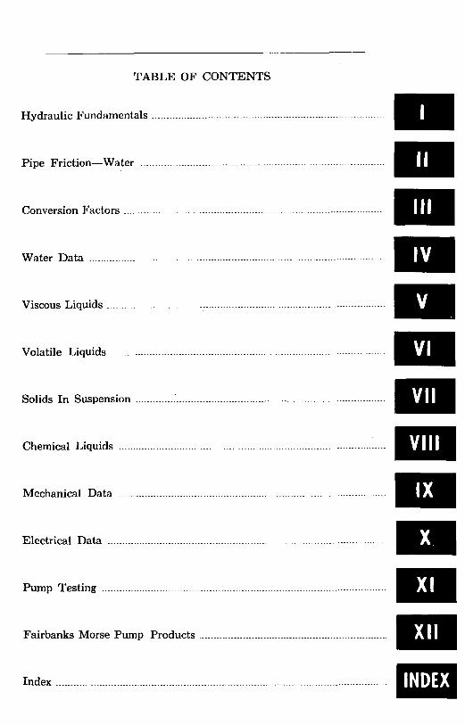
TABLE OF CONTENTS
Hydraulic Fundamentals ................................................................................
Pipe Friction-Water ....................................................................................
Conversion Factors ..........................................................................................
Water Data ......................................................................................................
. . Viscous Liqmds ................................................................................................
. . Volatile Liquids ..............................................................................................
Solids In Suspension ............. : ........................................................................
. . Chemical Liquids ..........................................................................................
Mechanical Data ..........................................................................................
Electrical Data ..............................................................................................
Pump Testing ..................................................................................................
Fairbanks Morse Pump Products .................................................................
Index ..................................................................................................................
6 H Y D R A U L I C H A N D B O O K
ACKNOWLEDGEMENTS In compiling the “Hydraulic Handbook.” we used pertinent data from many sources. We sincerely appreciate the courtesies, extended and are happy to give credit as follows: For copyrighted material from the Standards of the Hydraulic Institute,
10th Edition, 1964, and Pipe Friction Manual, Third Edition, 1961, 122 East 42nd Street, New York, N.Y.
Various Tables from “Cameron Hydraulic Data”-Ingersoll-Rand Com- pany, New York, N.Y.
American Standard Cast Iron Pipe Flanges and Flanged Fittings, (ASA B16b2-1931, B16.1-1948, B16b-1944 and B16bl-l931)-with the permis- sion of theAmerican Society of Mechanical Engineers, 29 West 39th Street, New York, N.Y.
“Domestic and Industrial Requirements” from “Willing Water #25”, December 1953-American Water Works A S S O C ~ Q ~ ~ O ~ , New York, N.Y.
Illustrations of gauges-United States Gauge Division of American Machine & Metals, Znc. Sellersville, Pa.
Approximate pH values from “Modern pH and Chlorine Control”-W. A. Taylor & Company, Baltimore, Md.
“Viscosity Temperature Chart”-Byron Jackson Company, Los Angeles, California.
Nozzle discharge tables from “Hydraulic Tables #31”-Factory Mutual Engineering Division, Associated Factory Mutual Fire Insurance Com- panies, Boston, Mass.
Chart “Vapor Pressure Versus Temperature For Motor and Natural Gas- oline”-Chicago Bridge & Iron Company, Chicago, Ill.
Chart “Vapor Pressure Propane-Butane Mixture” - Phillips Petroleum Company, Bartlesville, Okla.
Table of the selection and horsepower rating of V-belt drives-Dayton Rubber Manufacturing Co., Dayton, Ohio.
Text on Parallel and Series Operation-De Laud Steam Turbine Com- pany. Trenton, New Jersey.
Tables of Cast Iron Pipe Dimensions-Cast Iron Pipe Research ASSO&- tion, Chicago, Illinois.
“Infiltration Rates of Soils”-F. L. Duley and L. L. Kelly, S.C.S. Nebraska Experiment Station, Research Bulletin #12, and “Peak Moisture Use for Common Irrigated Crops and Optimum Yields”-A. W. McCullock, S.C.S. Reprinted from the Sprinkler Irrigation Handbook of the NQ- tional Rain Bird Sales & Engineering Corp, Azusa, Calif.
Food Pumping Installation from Hydro Pump Bulletin-Chisholm Ryder Company,, Inc., Niagara Falls, N.Y.
Text from “Pumps” by Kristal and Annett and “Piping Handbook” by Walker & Crocker-by permission of McGraw-Hill Book Co., Inc., New York, N.Y.
Data from “Handbook of Water Control”4alco Division, Armco Drain- age & Metal Products, Inc., Berkeley, Calif.
Illustration of Mechanical Seal-Durametallic Corporation, Kalamazoo, Michigan.
“Conversion Table for Approximate Hardness Numbers Obtained by Dif- ferent Methods”--from “Handbook of Engineering Fund.umentak”-- John Wiley & Sons, New York. N.Y.
H Y D R A U L I C F U N D A M E N T A L S 7
SECTION I-HYDRAULIC FUNDAMENTALS
CONTENTS Page
Hydraulics .......................................................................................... 8
Liquids In Motion ............................................................................ 9
Total Head .......................................................................................... 9
Fluid Flow .......................................................................................... 11
Water Hammer .................................................................................. 11
Specific Gravity And Head ............................................................ 14
Power, Efficiency, Energy .............................................................. 15
Specific Speed ..................................................................................... :16
Net Positive Suction Head .............................................................. 21
Cavitation ............................................................................................ 24
Siphons .................................................................................................. 25
Affinity Laws ...................................................................................... 27
Centrifugal Pumps-Parallel And Series Operation ................ 33
Hydro-Pneumatic Tanks ................................................................ 35
Corrosion .............................................................................................. 37
Galvanic Corrosion .............................................................................. 37
Non-Metallic Construction Materials ............................................. 40
Graphitization .................................................................................... 40
8 H Y D R A U L I C H A N D B O O K
SECTION I - HYDRAULIC FUNDAMENTALS
HYDRAULICS
The science of hydraulics is the study of the behavior of liquids at rest and in motion. This handbook concerns itself only with in- formation and data necessary to aid in the solution of problems in- volving the flow of liquids : viscous liquids, volatile liquids, slurries and in fact almost any of the rapidly growing number of liquids that can now be successfully handled by modern pumping machinery.
In a liquid at rest, the absolute pressure existing a t any point consists of the weight of the liquid above the point, expressed in psi, plus the absolute pressure in psi exerted on the surface (atmospheric pressure in an open vessel). This pressure is equal in all directions and exerts itself perpendicularly to any surfaces in contact with the liquid. Pressures in a liquid can be thought of as being caused by a column of the liquid which, due to its weight, would exert a pres- sure equal to the pressure at the point in question. This column of the liquid, whether real or imaginary, is called the static head and is usually expressed in feet of the liquid.
Pressure and head are, therefore, different ways of expressing the same value. In the vernacular of the industry, when the term “pres- sure” is used it generally refers to units in psi, whereas “head” refers to feet of the liquid being pumped. These values are mutually con- vertible, one to the other, as follows :
psi 2*31 = Head in feet. sg.
Convenient tables for making this conversion for water will be found in Section 111. Table 13 of this Handbook.
Pressure or heads are most commonly measured by means of a pressure gauge. The gauge measures the pressure above atmospheric pressure. Therefore, absolute pressure (psia) = gauge pressure (psig) plus barometric pressure (14.7 psi at sea level).
Since in most pumping problems differential pressures are used, gauge pressures as read and corrected are used without first convert- ing to absolute pressure.
H Y D R A U L I C F U N D A M E N T A L S 9
LIQUIDS I N MOTION
W Pumps are used to move liquids.
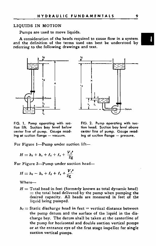
A consideration of the heads required to cause flow in a system and the definition of the terms used can best be understood by referring to the following drawings and text.
FIG. 1. Pump operating with suc- FIG. 2. Pump operating with suc- tion lift. Suction bay level below tion head. Suction bay level above center line of pump. Gauge read- center line of pump. Gauge read- ing at suction flange - vacuum. ing a t suction flange - pressure.
For Figure 1-Pump under suction lift-
For Figure 2-Pump under suction head-
Where-
H = Total head in feet (formerly known as total dynamic head) = the total head delivered by the pump when pumping the desired capacity. All heads are measured in feet of the liquid being pumped.
h d = Static discharge head in feet = vertical distance between the pump datum and the surface of the liquid in the dis- charge bay. The datum shall be taken at the centerline of the pump for horizontal and double suction vertical pumps or a t the entrance eye of the first stage impeller for single suction vertical pumps.
10 H Y D R A U L I C H A N D B O O K
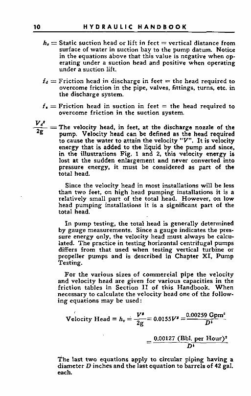
h, = Static suction head or lift in feet = vertical distance from surface of water in suction bay to the pump datum. Notice in the equations above that this value is negative when op- erating under a suction head and positive when operating under a suction lift.
f a = Friction head in discharge in feet = the head required to overcome friction in the pipe, valves, fittings, turns, etc. in the discharge system.
f, =Frict ion head in suction in feet = the head required to overcome friction in the suction system.
-- vds -The velocity head, in feet, at the discharge nozzle of the 2g pump. Velocity head can be defined as the head required
to cause the water to attain the velocity V". I t is velocity energy that is added to the liquid by the pump and since, in the illustrations Fig. 1 and 2, this velocity energy is lost a t the sudden enlargement and never converted into pressure energy, it must be considered as part of the total head.
Since the velocity head in most installations will be less than two feet, on high head pumping installations it is a relatively small part of the total head. However, on low head pumping installations it is a significant part of the total head.
In pump testing, the total head is generally determined by gauge measurements. Since a gauge indicates the pres- sure energy only, the velocity head must always be calcu- lated. The practice in testing horizontal centrifugal pumps differs from that used when testing vertical turbine or propeller pumps and is described in Chapter XI, Pump Testing.
For the various sizes of commercial pipe the velocity and velocity head are given for various capacities in the friction tables in Section I1 of this Handbook. When necessary to calculate the velocity head one of the follow- ing equations may be used:
V' 0.00259 Gpm2 D' Velocity Head = h, = -= 0.0155V' =
2g
- 0.00127 (Bbl. per Hour)* -. D4
The last two equations apply to circular piping having a diameter D inches and the last equation to barrels of 42 gal. each.
H Y D R A U L I C F U N D A M E N T A L S 11
FLUID F L O W
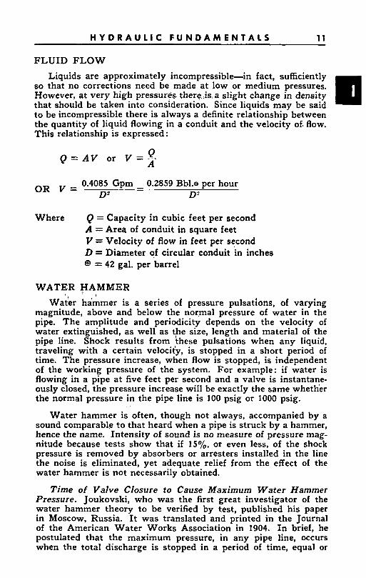
a Liquids are approximately incompressible-in fact, sufficiently so that no corrections need be made at low or medium pressures. However, a t very high pressures there ,is, a slight change in density that should be taken into consideration. Since liquids may be said to be incompressible there is always a definite relationship between the quantity of liquid flowing in a conduit and the velocity of. flow. This relationship is expressed :
e Q = A V or V = - A
0.4085 Gpm - 0.2859 Bb1.a per hour - D2 D' OR V =
Where Q = Capacity in cubic feet per second A = Area of conduit in square feet V = Velocity of flow in feet per second D = Diameter of circular conduit in inches @ = 42 gal. per barrel
WATER HAMMER
Wader hammer is a series of pressure pulsations, of varying magnitude, above and below the normal pressure of water in the pipe. The amplitude and periodicity depends on the velocity of water extinguished, as well as the size, length and material of the pipe line. Shock results from these pulsations when any Iiquid, traveling with a certain velocit'y, is stopped in a short period of time. The pressure increase, when flow is stopped, is independent of the working pressure of the system. For example: if water is flowing in a pipe at five feet per second and a valve is instantane- ously closed, the pressure increase will be exactly the same whether the normal pressure in the pipe line is 100 psig or 1000 psig.
Water hammer is often, though not always, accompanied by a sound comparable to that heard when a pipe is struck by a hammer, hence the name. Intensity of sound is no measure of pressure mag- nitude because tests show that if 15%, or even less, of the shock pressure is removed by absorbers or arresters installed in the line the noise is eliminated, yet adequate relief from the effect of the water hammer is not necessarily obtained.
Time of Valve Closure to Cause Maximum Water Hammer Pressure. Joukovski, who was the first great investigator of the water hammer theory to be verified by test, published his paper in Moscow, Russia. It was translated and printed in the Journal of the American Water Works Association in 1904. In brief, he postulated that the maximum pressure, in any pipe line, occurs when the total discharge is stopped in a period of time, equal or
* ' ,
12 H Y D R A U L I C H A N D B O O K
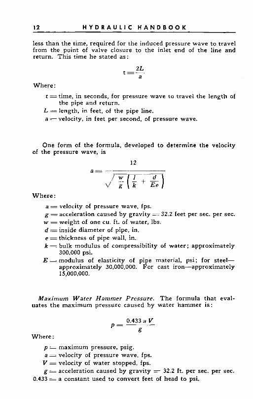
less than the time, required for the induced pressure wave to travel from the point of valve closure to the inlet end of the line and return. This time he stated as:
Where :
t = time, in seconds, for pressure wave to travel the length of the pipe and return.
L =length, in feet, of the pipe line. a =velocity, in feet per second, of pressure wave.
One form of the formula, developed to determine the velocity of the pressure wave, is
12 a -
d’-) Where:
a = velocity of pressure wave, fps. g = acceleration caused by gravity = 32.2 feet per sec. per sec. w =weight of one cu. ft. of water, lbs. d = inside diameter of pipe, in. e = thickness of pipe wall, in. k = bulk modulus of compressibility of water ; approximately
300,000 psi. E =modulus of elasticity of pipe material, psi; for steel-
approximately 30,000,000. For cast iron-approximately 15,000,000.
Maximum Water Hammer Pressure. The formula that eval- uates the maximum pressure caused by water hammer is:
0.433 a V g
P =
Where :
p = maximum pressure, psig. a = velocity of pressure wave, fps. V = velocity of water stopped, fps. g = acceleration caused by gravity = 32.2 f t . per sec. per sec.
0.433 = a constant used to convert feet of head to psi.
H Y D R A U L I C F U N D A M E N T A L S 13
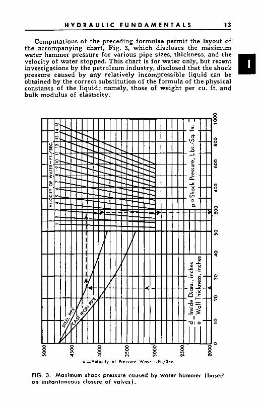
Computations of the preceding formulae permit the layout of the accompanying chart, Fig. 3, which discloses the maximum water hammer pressure for various pipe sizes, thickness, and the velocity of water stopped. This chart is for water only, but recent investigations by the petroleum industry, disclosed that the shock pressure caused by any relatively incompressible liquid can be obtained by the correct substitution of the formula of the physical constants of the liquid; namely, those of weight per cu. ft. and bulk modulus of elasticity.
W
o z V e l o c i t y of Pressure Wove-Ft./Sec.
FIG. 3. Maximum shock pressure caused by water hammer (based on instantaneous closure of valves).
14 H Y D R A U L I C H A N D B O O K
Example : What is the maximum pressure caused by water hammer in an
b-inch steel pipe line (0.322-inches wall thickness) transporting water a t a steady velocity of 3 fps?
Procedure in Using Chart:
-- - 24.8. d inside dia. of pipe, in. - 7.981 e wall thickness of pipe, in. 0.322
Determine the ratio - = -
d e Enter the chart a t - = 24.8 and project upward to the intersec-
tion with the line for steel pipe. Note that the value of the velocity of the pressure wave, a =
4225 fps. Project horizontally to the right, to an intersection with the 3
fps. velocity line and then down to the base line, where shock pres- sure of 170 psi is obtained.
SPECIFIC GRAVITY AND H E A D
peripheral velocity of the impeller. It is expressed thus:
-
The head developed by a centrifugal pump depends upon the
Where H = Total Head at zero capacity developed by the pump in feet
u = Velocity at periphery of impeller in feet per second
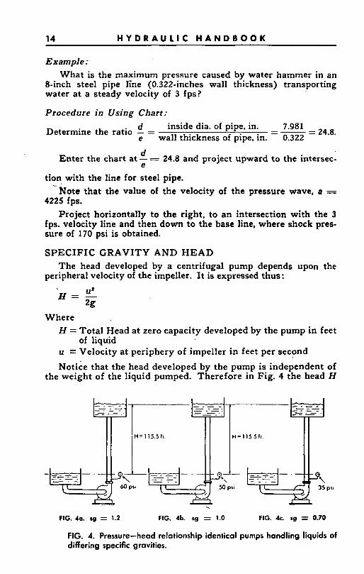
Notice that the head developed by the pump is independent of the weight of the liquid pumped. Therefore in Fig. 4 the head H
of liquid
15.511
. FIG. 4a. sg = 1.2 FIG. 4b. rg = 1.0 FIG. G. sg = 0.70
FIG. 4. Pressure-head relationship identical pumps handling liquids of differing specific gravities.
H Y D R A U L I C F U N D A M E N T A L S 15
in feet would be the same whether the pump was handling water with a specific gravity of 1.0, gasoline with a sg. of 0.70, brine of a sg. of 1.2 or a fluid of any other specific gravity. The pressure reading on the gauge, however, would differ although the im- peller diameter and. speed is identical'in each case.
H X sg. 2.31 The gauge reading in psi =
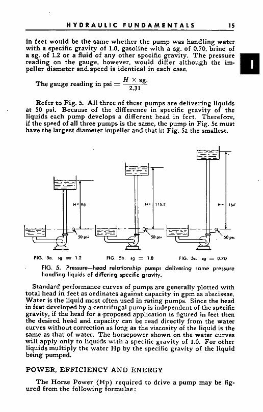
Refer to Fig. 5. All three of these pumps are delivering liquids a t 50 psi. Because of the difference in specific gravity of the liquids each pump develops a different head in feet. Therefore, if the speed of all three pumps is the same, the pump in Fig. 5c must have the largest diameter impeller and that in Fig. Sa the smallest.
1 15.5' I+=
A-
-
164'
-
FIG. 5b. sg = 1.0 FIG. 5c. sg = 0.70 FIG. 50. sg = 1.2
FIG. 5. Pressure-head relationship pumps delivering same pressure handling liquids of differing specific gravity.
Standard performance curves of pumps are generally plotted with total head in feet as ordinates against capacity in gpm as abscissae. Water is the liquid most often used in rating pumps. Since the head in feet developed by a centrifugal pump is independent of the specific gravity, if the head for a .proposed application is figured in feet then the desired head and capacity can be read directly from the water curves without correction as long as the viscosity of the liquid is the same as that of water. The horsepower shown on the water curves will apply only to liquids with a specific gravity of 1.0. For other liquids multiply the water H p by the specific gravity of the liquid being pumped.
POWER, EFFICIENCY AND ENERGY
ured from the following formulae : The Horse Power (Hp) required to drive a pump may be fig-
16 H Y D R A U L I C H A N D B O O K
Liquid Hp or useful work done by the pumps = lbs. of liquid raised per min. x H in feet
33,000 Whp =
- gpm X H, f t . X sg. 3960
-
The Brake Horsepower required to drive the pump = gpm X H, f t . X sg. 3960 X Pump Eff, Bhp =
Output Whp Input Bhp
Pump Efficiency = --- - ~
Electrical Hp input to Motor = BhP Motor Eff.
- Gpm X H, ft. X sg. 3960 x Pump Eff. x Motor Eff.
-
Bhp X 0.746 Motor Eff.
Kw input to Motor =
- Gpm X H, f t . X sg. X 0.746 3960 X Pump Eff. X Motor Eff.
-
Overall Eff. = Pump Eff. x Motor Eff.
H, ft. X 0.00315 Overall Eff.
Kwh per 1000 gal. water pumped =
Kwh per 1000 gal. water pumped = K x H
Where K = a constant depending upon the overall efficiency of the pumping unit obtained from Table 15 in Section 111.
SPECIFIC SPEED
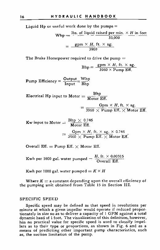
Specific speed may be defined as that speed in revolutions per minute a t which a given impeller would operate if reduced propor- tionately in size so as to deliver a capacity of 1 GPM against a total dynamic head of 1 foot. The visualization of this definition, however, has no practical value for specific speed is used to classify impel- lers as to their type or proportions, as shown in Fig. 6 and as a means of predicting other important pump characteristics, such as, the suction limitation of the pump.
H Y D R A U L I C F U N D A M E N T A L S 17
Ns 500 TO 3000 1000 TO 3500 1500 TO 4500 4500 TO no00 0000 6 UP TYPE RADIAL DOUBLE SUCTION FRANCIS MIXEDFLOW FRANCIS PROPELLER
HEAD ABOVE 150' ABOVE 100' 65' TO 150' 35' 10 65, 1' 10 4v D,;D,=2+ I .5 1.5 1.3-1.1 1 .o
FIG. 6. Relation specific speeds, N,, to pump proportions, - D:! D1
v z
800
600
200
100
BO
60
B 40
LI 0
z 20 I n
10 i!
8
b
A
2
I
BMX)
MKK)
4000
lo00
Boo
100
80
60
A0
10
1 2 4 b 8 1 0 20 A 0 60 80 100 200
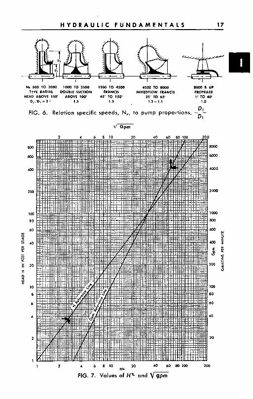
FIG. 7. Values of H % and v gpm Hi
~

18 H Y D R A U L I C H A N D B O O K
SPECIFIC SPEED-SUCTION LIMITATIONSf
Among the more important factors affecting the operation of a centrifugal pump are the suction conditions. Abnormally high suction lifts (low NPSH) beyond the suction rating of the pump, usually causes serious reductions in capacity and efficiency, and often leads to serious trouble from vibration and cavitation.
Specific Speed. The effect of suction lift on a centrifugal pump is related to its head, capacity and speed. The relation of these factors for design purposes is expressed by an index number known as the specific speed. The formula is as follows:
rpmd/gpm HS Specific Speed, N, =
where H = head per stage in feet (Fig. 7 shows the corresponding values of H% and gE'.
H'TOTAL HEAD IN FEET
8 8 8 8 4 8 Z 8 8 S 5 1 3 :: R
OL
!!
8
. . .
4000
3500
3000
2500
i 2000
g 1500
n
Y Z n 1700 n
,,, 1900
3
v)
2 4 1800
1600
' 1400
1300
1200
1100
6000
5500 Y)
I" 5000 a
z 4500 2
U
4000 2 3
a m
B 9
3500 OL
3000 ' e 2500
i
Ei YI
2000 % 1900 2 I800 = M 1700 % 1600
IS00
FIG. 8. Hydraulic institute upper limits of specific speeds for single stage, single suction and double suction pumps with shaft through eye of impeller pumping clear water at sea level at 85OF.
t Courtesy Hydraulic Institute. See page 6.
H Y D R A U L I C F U N D A M E N T A L S 19
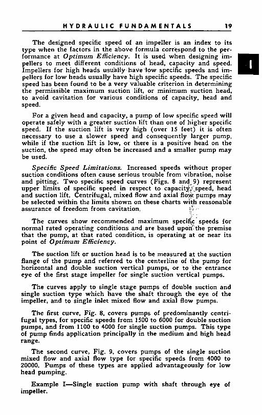
The designed specific speed of an impeller is an index to its type when the factors in the above formula correspond to the per- formance at Optimum Efficiency. It is used when designing im- pellers to meet different conditions of head, capacity and speed. Impellers for high heads usually have low specific speeds and im- pellers for low heads usually have high specific speeds. The specific speed has been found to be a very valuable criterion in determining the permissible maximum suction lift, or minimum suction head, to avoid cavitation for various conditions of capacity, head and speed.
For a given head and capacity, a pump of low specific speed will operate safely with a greater suction lift than one of higher specific speed. If the suction lift is very high (over 15 feet) it is often necessary to use a slower speed and consequently larger pump, while if the suction lift is low, or there is a positive head on the suction, the speed may often be increased and a smaller pump may be used.
Specific Speed Limitations. Increased speeds without proper suction conditions often cause serious trouble from vibration, noise and pitting. Two specific speed curves (Figs. 8 andz+9) represent upper limits of specific speed in respect to capacity,:speed, head and suction lift. Centrifugal, mixed flow and axial flow pumps may be selected within the limits shown on these charts with reasonable assurance of freedom from cavitation.
m
i'.
The curves show recommended maximum specific. speeds for normal rated operating conditions and are based upodthe premise that the pump, a t that rated condition, is operating at or near its point of Optimum Efficiency.
The suction lift or suction head is to be measured at the suction flange of the pump and referred to the centerline of the pump for horizontal and double suction vertical pumps, or to the entrance eye of the first stage impeller for single suction vertical pumps.
The curves apply to single stage pumps of double suction and single suction type which have the shaft through the eye of the impeller, and to single inlet mixed flow and axial flow pumps.
The first curve, Fig. 8, covers pumps of predominantly centri- fugal types, for specific speeds from 1500 to 6000 for double suction pumps, and from 1100 to 4000 for single suction pumps. This type of pump finds application principally in the medium and high head range.
The second curve, Fig. 9, covers pumps of the single suction mixed flow and axial flow type for specific speeds from 4000 to 20000. Pumps of these types are applied advantageously for low head pumping.
Example I-Single suction pump with shaft through eye of impeller.
20 H Y D R A U L I C H A N D B O O K
100 20000
15000
8000
7000
6000
5000
4000
H=TOTAL HEAD IN FEET
50 40 30 20 15 1 0 9 8 7 6
100 50 40 30 20 15 i o 9 a 7 6 5
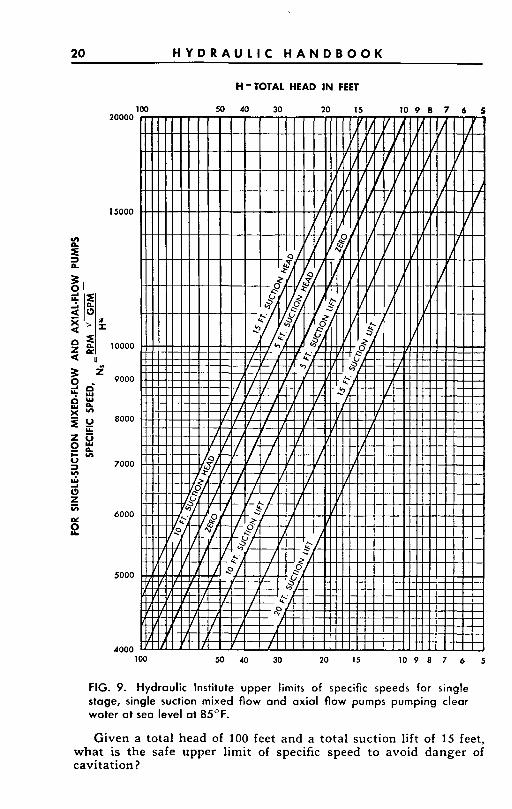
FIG. 9. Hydraulic Institute upper limits of specific speeds for single stage, single suction mixed flow and axial flow pumps pumping clear water a t sea level at 85OF.
Given a total head of 100 feet and a total suction lift of 15 feet, what is the safe upper limit of specific speed to avoid danger of cavitation?
H Y D R A U L I C F U N D A M E N T A L S 21
Referring to Fig. 8, the intersection, of the diagonal for 15 feet suction lift with the vertical line at total pump head of 100 feet, falls on the horizontal line corresponding -to 2250 specific speed. The specific speed should not exceed this value.
Example 11-Double suction pump.
Given a total head of 100 feet and a total suction lift of 15 feet, what is the safe upper limit of specific speed?
Referring to the first curve, Fig. 8, the intersection, of the diagonal for 15 feet suction lift with the vertical line for 100 feet total pump head, falls on the horizontal line corresponding to 3200 specific speed on the scale a t the right side of the chart. This is the value of
‘PmVgPm ~ N , H’.
in which the volume, or gpm, is the total gallons per minute capac- ity of the pumping unit including both suctions ; and is the highest value which should be used for this head and suckion lift.
Example 111-Single suction mixed flow or axial flow pump.
Given a total head of 35 feet and a total suction head of 10 feet, corresponding to a submerged impeller, what is the safe upper limit of specific speed?
Referring to the second curve, Fig. 9, the intersection, of the vertical line for 35 feet total pump head and the diagonal for 10 feet suction head, falls on the horizontal line corresponding to 9400 specific speed on the scale a t the left side of the chart. The specific speed should not exceed this value.
NET POSITIVE SUCTION HEAD (NPSH)
NPSH can.be defined as the.head that causes liquid to flow through the suction piping and finally enter the eye of the impeller.
This head that causes flow comes from either the pressure of the atmosphere or from static head plus atmospheric pressure. A pump operating under a suction lift has as a source of pressure to cause flow only the pressure of the atmosphere. The work that can be done, therefore, on the suction side of a pump is limited, so NPSH becomes very important to the successful operation of the pump. There are two values of NPSH to consider.
REQUIRED NPSH is a function of the pump design. I t varies between different makes of pumps, between different pumps of the same make and varies with the capacity and speed of any one pump. This is a value that must be supplied by the maker of the pump.
AVAILABLE NPSH is a function of the system in which the pump operates. I t can be calculated for any installation. Any pump installation, to operate successfully, must have an available NPSH
22 H Y D R A U L I C H A N D B O O K
equal to or greater than the required NPSH of the pump at the desired pump conditions.
When the source of liquid is above the pump:
NPSH = Barometric Pressure, Ft. + Static Head on suction, ft. - friction losses in suction piping, ft. - Vapor Pressure of liquid, f t .
When the source of liquid is below the pump:
NPSH = Barometric Pressure, ft. - Static Suction lift, ft. - friction losses in Suction piping, ft. - Vapor Pres- sure of liquid, ft.
To illustrate the use of these equations consider the following examples :
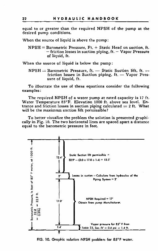
The required NPSH of a water pump at rated capacity is 17 ft. Water Temperature 8S°F. Elevation 1000 ft. above sea level. En- trance and friction losses in suction piping calculated = 2 ft. What will be the maximum suction lift permissible?
To better visualize the problem the solution is presented graphi- cally in Fig. 10. The two horizontal lines are spaced apart a distance equal to the barometric pressure in feet.
FIG. 10. Graphic solution NPSH problem for 85°F water.
H Y D R A U L I C F U N D A M E N T A L S 23
I 0 0 0
(22.3 + 17.0 + 2k33.8 5 7.5 h.
7.c ot Suction Flonge = piping system = 2'
L - 0
D I I 0 a - r 0 L
0 0 e I I C .- I I
FIG. 11. Graphic solution NPSH problem for 1W0F water.
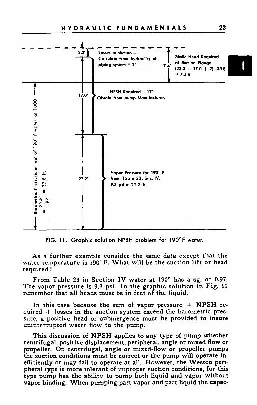
As a further example consider the same data except that the water temperature is 19O0F. What will be the suction lift or head required ?
From Table 23 in Section IV water at 190' has a sg. of 0.97. The vapor pressure is 9.3 psi. I n the graphic solution in Fig. 11 remember that all heads must be in feet of the liquid.
In this rase because the sum of vapor pressure + NPSH re- quired + losses in the suction system exceed the barometric pres- sure, a positive head or submergence must be provided to insure uninterrupted water flow to the pump.
This discussion of NPSH applies to any type of pump whether centrifugal, positive displacement, peripheral, angle or mixed flow or propeller. On centrifugal, angle or mixed-fow or propeller pumps the suction conditions must be correct or the pump will operate in- efficiently or may fail to operate at all. However, the Westco peri- pheral type is more tolerant of improper suction conditions, for this type pump has the ability to pump both liquid and vapor without vapor binding. When pumping part vapor and part liquid the capac-
24 H Y D R A U L I C H A N D B O O K
ity is, of course, reduced. Advantage is taken of the suction toler- ance of this pump and it is frequently installed under suction condi- tions quite impossible for a centrifugal pump. The manufacturer can supply ratings of their pumps under these adverse conditions.
CAVITATION
Cavitation is a term used to describe a rather complex phenome- non that may exist in a pumping installation. In a centrifugal pump this may be explained as follows. When a liquid flows through the suction line and enters the eye of the pump impeller an increase in velocity takes place. This increase in velocity is, of course, accompanied by a reduction in pressure. If the pressure falls below the vapor pressure corresponding to the temperature of the liquid, the liquid will vaporize and the flowing stream will consist of liquid plus pockets of vapor. Flowing further through the impel- ler, the liquid reaches a region of higher pressure and the cavities of vapor collapse. I t is this collapse of vapor pockets that causes the noise incident to cavitation.
Cavitation need not be a problem in a pump installation if the pump is properly designed and installed, and operated in accordance with the designer's recommendations. Also, cavitation is not neces- sarily destructive. Cavitation varies from very mild to very severe. A pump can operate rather noiselessly yet be cavitating mildly. The only effect may be a slight drop in efficiency. On the other hand severe cavitation will be very noisy and will destroy the pump im- peller and/or other parts of the pump.
Any pump can be made to cavitate, so care should be taken in selecting the pump and planning the installation. For centrifugal pumps avoid as much as possible the following conditions :
1. Heads much lower than head at peak efficiency of pump.
2. Capacity much higher than capacity at peak efficiency of Pump.
3. Suction lift higher or positive head lower than recommended by manufacturer.
4. Liquid temperatures higher than that for which the system was originally designed.
5. Speeds higher than manufacturer's recommendation.
The above explanation of cavitation in centrifugal pumps can- not be used when dealing with propeller pumps. The water entering a propeller pump in a large bell-mouth inlet will be guided to the smallest section, called throat, immediately ahead of the propeller. The velocity there should not be excessive and should provide a suf- ficiently large capacity to fill properly the ports between the pro- peller blades. As the propeller blades are widely spaced, not much guidance can be given to the stream of water. When the head is in-
H Y D R A U L I C F U N D A M E N T A L S 25
creased beyond a safe limit, the capacity is reduced to a quantity in- sufficient to fill up the space between the propeller vanes. The stream of water will separate from the propeller vanes, creating a small space where pressure is close to a perfect vacuum. I n a very small fraction of a second, this small vacuum space will be smashed by the liquid hitting the smooth surface of the propeller vane with an enor- mous force which starts the process of surface pitting of the vane. At the same time one will hear a sound like rocks thrown around in a barrel or a mountain stream tumbling boulders.
n The five rules applying to centrifugal pumps will be changed to
suit propeller pumps in the following way: Avoid as much as possi- ble,
1. Heads much higher than at peak efficiency of pump.
2. Capacity much lower than capacity at peak efficiency of Pump.
3. Suction lift higher or positive head lower than recom- mended by manufacturer.
4. Liquid temperatures higher than that for which the system was originally designed.
5. Speeds higher than manufacturer’s recommendation.
Cavitation is not confined to pumping equipment alone. It also occurs in piping systems where the liquid velocity is high and the pressure low. Cavitation should be suspected when noise is heard in pipe lines at sudden enlargements of the pipe cross-section, sharp bends, throttled valves or like situations.
SIPHONS
I t occasionally happens that a siphon can be placed in the dis- charge line so that the operating head of a pump is reduced. The re- duction in head so obtained will lower the power costs for lifting a given amount of water and may make possible, in addition, the in- stallation of a smaller pumping unit.
Successful operation of such a combination demands that the pump and siphon be designed as a unit under the following limita- tions.
1. In order to prime the siphon in starting, the pump must be able to deliver a full cross-section of water to the throat, or peak, of the siphon against the total head of that elevation and with a mini- mum velocity of five feet per seeond.
26 H Y D R A U L I C H A N D B O O K
TEMPERATURE OF WATER IN OF.
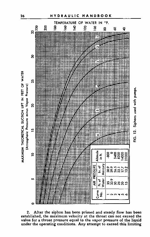
2. After the siphon has been primed and steady flow has been established, the maximum velocity at the throat can not exceed the value for a throat pressure equal to the vapor pressure of the liquid under the operating conditions. Any attempt to exceed this limiting
H Y D R A U L I C F U N D A M E N T A L S 27
velocity will result in “cavitation,” or vaporization of the liquid, under the reduced Dressure.
U The theoretical pressure drop can be obtained from the curves in Fig. 12 which ar.e based on the standard atmosphere as defined bv the U. S. Bureau of Standards in its Dublication #82. A safe Glue for design purposes may be obtained directly from the curve for 75% of the actual atmospheric pressure. This value may be used as an estimate of the possible head reduction by the use of a siphon providing a reasonable allowance for friction losses is de- ducted from it.
The pipe section at the throat must be designed to resist the external pressure caused by the reduction of pressure below that of the atmosphere.
In practically all cases it is advisable that the discharge end of the siphon be sufficiently submerged to prevent the entrance of air. The exit losses at this point can be reduced by belling the end of the pipe and thus recovering a large part of the velocity head.
3.
4.
AFFINITY LAWS-CENTRIFUGAL PUMPS .:**
U. s. GALLONS PER MNUTE
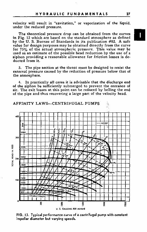
FIG. 13. Typical performance curve of a centrifugal pump with constant impeller diameter but varying speeds.
28 H Y D R A U L I C H A N D B O O K
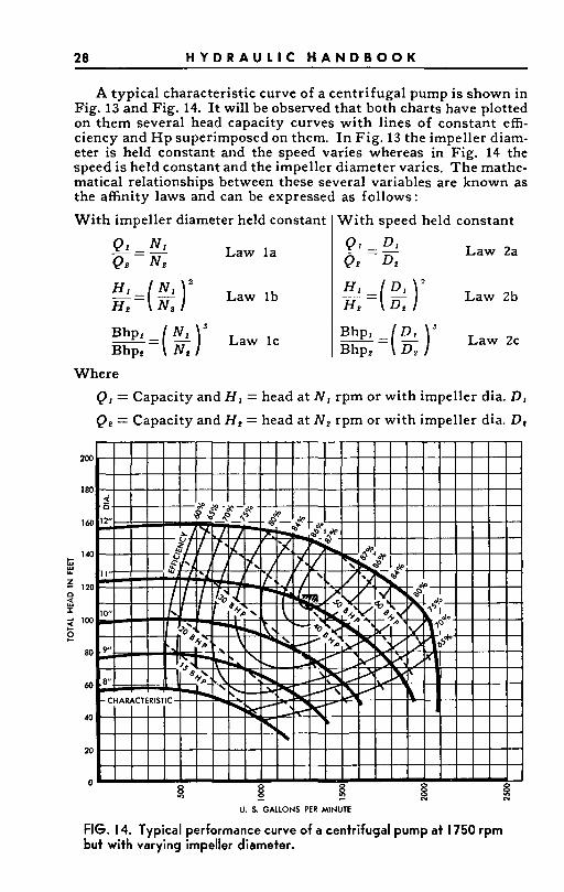
A typical characteristic curve of a centrifugal pump is shown in Fig. 13 and Fig. 14. It will be observed that both charts have plotted on them several head capacity curves with lines of constant effi- ciency and H p superimposed on them. I n Fig. 13 the impeller diam- eter is held constant and the speed varies whereas in Fig. 14 the speed is held constant and the impeller diameter varies. The mathe- matical relationships between these several variables are known as the affinity laws and can be expressed as follows:
Wi th impeller diameter held constant I With speed held constant
Law 2a
Where Q1 = Capacity and H I = head at N, rpm or with impeller dia. D, Qp = Capacity and He = head at N, rpm or with impeller dia. D,
U. 5. GALLONS PER MINUTE
FIG. 14. Typical performance curve of a centrifugal pump at I750 rpm but with varying impeller diameter.
H Y D R A U L I C F U N D A M E N T A L S 29
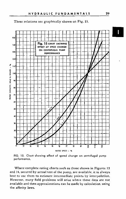
These relations are graphically shown on Fig. 15.
RATED SPEED - %
FIG. 15. Char t showing effect of speed change on centrifugal pump performance.
Where complete rating charts such as those shown in Figures 13 and 14, secured by actual test of the pump, are available, it is always best to use them to estimate intermediate points by interpolation. However, many field problems will arise where these data are not available and then approximations can be made by calculation, using the affinity laws.
30 H Y D R A U L I C H A N D B O O K
Law l a applies to Centrifugal, Angle Flow, Mixed Flow, Pro-
Law l b and c apply to Centrifugal, Angle Flow, Mixed Flow,
Law Za, b, c apply to Centrifugal pumps only.
peller, Peripheral, Rotary and Reciprocating pumps.
Propeller, and Peripheral pumps.
Examples illustrating the use of these laws follow. Note particu- larly from these examples that the calculated head-capacity char- acteristic using Law 1 agrees very closely to the test performance curves. However, this i s true for Law 2 only under certain defined conditions. Law 2 must, therefore, be used with a great deal of caution.
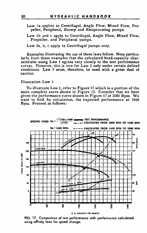
Illustration Law 1
To illustrate Law 1, refer to Figure 17 which is a portion of the more complete curve shown in Figure 13. Consider that we have given the performance curve shown in Figure 17 at 2000 Rpm. We want to find, by calculation, the expected performance at 1600 Rpm. Proceed as follows:
V m x 1600 - TEST PERFORMANCE SPEED N'- (1lS)C --- CALCULATED FROM 2000 RPM TO 1600 RPM
Ns- 1680 RPM ---- CALCULATED FROM 1600 RPM TO 2000 RPM
U. 5 GALLONS PER MINUTE
FIG. 17. Comparison of test performance with performance calculated using offinity laws for speed change.
H Y D R A U L I C F U N D A M E N T A L S 31
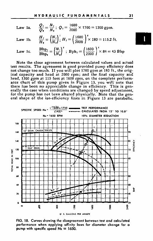
l6O0 X 1700 = 1360 gpm. 91 - N1 - - N, ; Q 1 = 2000 9 8
5 = (2); HI = ( ”””-) ‘X 180 = 115.2 ft. HI 2000
Law la.
Law Ib.
Note the close agreement between calculated values and actual test results. The agreement is good provided pump efficiency does not change too much. If you will plot 1700 gpm at 180 ft., the orig- inal capacity and head at 2000 rpm; and the final capacity and head, 1360 gpm at 115 feet at 1600 rpm, on the complete perform- ance chart of this pump given in Figure 13, you will.note that there has been no appreciable change in efficiency. This is gen- erally the case when conditions are changed by speed adjustment, for the pump has not been altered physically. Note that the gen- eral shape of the iso-efficiency lines in Figure 13 are parabolic.
140
t 120
E n 100
1
m
40
0
F U
‘y u Y
U 5. GALLONS PER MINUTE
FIG. 18. Curves showing the disagreement between test and calculated performance when applying affinity laws for diameter change for a pump with specific speed Ns = 1650.
32 H Y D R A U L I C H A N D B O O K
Therefore, the curve A-B in Fig. 17 passing through the two con- dition points on the 2000 rpm and 1600 Rpm curves, which is also parabolic, is approximately parallel to the iso-efficiency curves. The use of the Affinity Laws, therefore, to calculate performance when the speed is changed and the impeller diameter remains con- stant, is a quite accurate approximation. By calculating several points along a known performance curve, a new performance curve can be produced showing the approximate performance a t the new speed.
Starting with the 1600 rpm characteristic and calculating the performance at 2000 rpm by the use of the affinity laws, the calcu- lated performance exceeds the actual performance as shown in dotted curve on Figure 17. The discrepancy is slight but empha- sizes the fact that the method is only a quite accurate approxima- tion.
U T 0 x 1750 TEST PERFORMANCE SPECIFIC SPEED Nr= (260)'
NS = 855 RPM - - - - - - - CALCULATED FROM 17%'' TO 14"
U. S GALLONS PER MINUTE
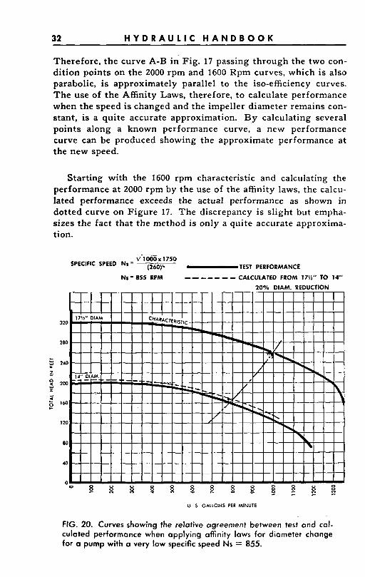
FIG. 20. Curves showing the relative agreement between test and cal- culated performance when applying affinity laws for diameter change for a pump with a very low specific speed Ns = 855.
H Y D R A U L I C F U N D A M E N T A L S 33
Illustration Law 2
W Probably this should not be considered as an affinity law, for when the impeller of a pump is reduced in diameter, the design relationships are changed, and in reality a new design results. Law 2, therefore, does not yield the accurate results of Law 1. It is always recommended that the pump manufacturer be con- sulted before changing the diameter of an impeller in the field.
. Figure 20 illustrates the comparative accuracy of test perform- ance to the calculated performance on a very low specific speed pump. Figure 18, however, shows rather wide discrepancy be- tween test and calculated results on a pump of higher specific speed. On pumps of still higher specific speed the lack of .agree- ment between test and calculated results is even more pronounced.
In general, agreement will be best on low specific speed pumps and the higher the specific speed the greater the disagreement. However specific speed is only one of the factors considered by the manufacturer when determining the proper impeller diameter.
When the affinity laws are used for calculating speed or diam- eter increases, it is important to consider the effect of suction l if t on the characteristic for the increased velocity in the suction line and pump may result in cavitation that may substantially alter the characteristic curve of the pump.
PARALLEL AND SERIES OPERATION*
When the pumping requirements are variable, it may be more de- sirable to install several small pumps in parallel rather than use a single large one. When the demand drops, one or more smaller pumps may be shut down, thus allowing the remainder to operate at or near peak efficiency. If a single pump is used with lowered de- mand, the discharge must be throttled, and it will operate at reduced efficiency. Moreover, when smaller units are used opportunity is pro- vided during slack demand periods for repairing and maintaining each pump in turn, thus avoiding plant shut-downs which would be necessary with single units. Similarly, multiple pumps in series may be used when liquid must be delivered a t high heads.
In planning such installations a head-capacity curve for the sys- tem must first be drawn. The head required by the system is the sum of the static head (difference in elevation and/or its pressure equivalent) plus the variable head (friction and shock losses in the pipes, heaters, etc.). The former is usually constant for a given system whereas the latter increases approximately with the square of the flow. The resulting curve is represented as line AB in Figs. 21 and 22.
tCourfery De h v a l Steam Turbine Co. See page 6.
34 H Y D R A U L I C H A N D B O O K
C
E
f
0 9, I
U-
A
F D I ” Static
Capacity, Q
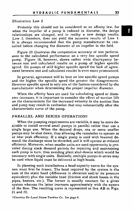
FIG. 21. Head capacity curves of pumps operating in parallel.t
Connecting two pumps in parallel to be driven by one motor is not a very common practice and, offhand, such an arrangement may appear more expensive than a single pump. However, it should be remembered that in most cases it is possible to operate such a unit at about 40 per cent higher speed, which may reduce the cost of the motor materially. Thus, the cost of two high-speed pumps may not be much greater than that of a single slow-speed pump.
For units to operate satisfactorily in parallel, they must be work- ing on the portion of the characteristic curve which drops off with increased capacity in order to secure an even flow distribution. Consider the action of two pumps operating in parallel. The system head-capacity curve AB shown in Fig. 21 starts a t H static when the flow is zero and rises parabolically with increased flow. Curve CD represents the characteristic curve of pump A operating alone ; the similar curve for pump B is represented by EF. Pump B will not start delivery until the discharge pressure of pump A falls below that of the shut-off head of B (point E). The combined delivery for a given head is equal to the sum of the individual capacities of the two pumps a t that head. For a given combined delivery head, the capac- i ty is divided between the pumps as noted on the figures Qd and Qe. The combined characteristic curve shown on the figure is found by plotting these summations. The combined brake horse- +Courtesy John Wiley & Sons, Inc. See page 6.
H Y D R A U L I C F U N D A M E N T A L S 35
I 4 '
Capocity, Q
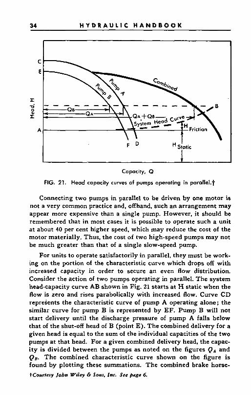
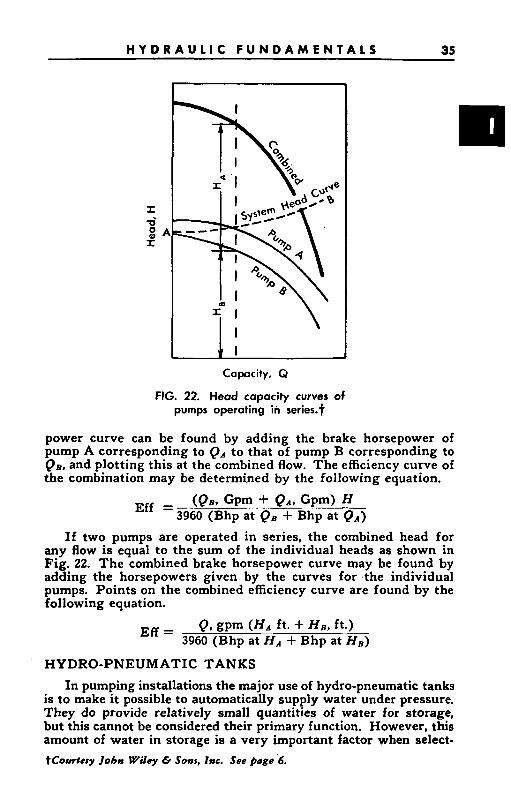
FIG. 22. Head capacity curves of pumps operating in series.f
power curve can be found by adding the brake horsepower of pump A corresponding to Q A to that of pump B corresponding to QB, and plotting this at the combined flow. The efficiency curve of the combination may be determined by the following equation.
(QB, Gpm + QA, Gpm) H 3960 (Bhp at Q B + Bhp at Q A ) Eff =
If two pumps are operated in series, the combined head for any flow is equal to the sum of the individual heads as shown in Fig. 22. The combined brake horsepower curve may be found by adding the horsepowers given by the curves for the individual pumps. Points on the combined efficiency curve are found by the following equation.
Q. gpm (HA ft . + He. ft-) 3960 (Bhp at HA + Bhp at Hs) Eff =
HYDRO-PNEUMATIC TANKS
In pumping installations the major use of hydro-pneumatic tanks is to make it possible to automatically supply water under pressure. They do provide relatively small quantities of water for storage, but this cannot be considered their primary function. However, this amount of water in storage is a very important factor when select- tCourtesy Jobn Wilcj, & Sons, Inc. See #age '6.
36 H Y D R A U L I C H A N D B O O K
ing the proper size tank to be used with the pump selected. The US- able storage capacity should be such that the pump motor will not start frequently enough to cause overheating. Starting 10 to 15 times per hour will usually be satisfactory. The limit in the number of starts per hour depends upon the motor horsepower and speed. For the higher speeds and horse-powers use less starts per hour.
I
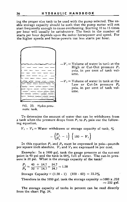
FIG. 23. Hydro-pneu- matic tank.
-V , = Volume of water in tank a t the High or Cut-Out pressure P I psia, in per cent of tank vol- ume.
~
-V, = Volume of water in tank at the Low or Cut-In pressure Pe psia, in per cent of tank vol- ume.
To determine the amount of water that can be withdrawn from a tank when the pressure drops from P I to Pp psia use the follow- ing equation.
V, - V e = Water withdrawn or storage capacity of tank, o/o
= (2 - 1) (100 - v, 1 I n this equation P, and P2 must be expressed in psia-pounds
per square inch absolute. V, and V 2 are expressed in per cent.
Example: In a 1000 gal. tank the gauge pressure at the cut-out point is 40 psi and the tank is 60% full of water. T h e cut-in pres- sure is 20 psi. What is the storage capacity of the tank?
Pi - 40 + 14.7 54.7 - = 1.58 - - - P , 20 -I- 14.7 - 34.7
Storage Capacity = (1.58 - 1)
Therefore in the 1000 gal. tank the storage capacity =lo00 x .232 = 232 gal.
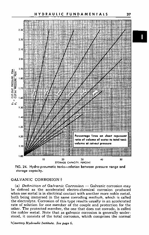
The storage capacity of tanks in percent can be read directly
(100 - 60) = 23.2%
from the chart Fig. 24.
H Y D R A U L I C F U N D A M E N T A L S 37
10 20 30 40 50 STORAGE CAPACITY, PERCENT
FIG. 24. Hydro-pneumatic tanks-relation between pressure range and storage capacity.
GALVANIC CORROSION f (a) Defini t ion of Galvanic Corrosion - Galvanic corrosion may
be defined as the accelerated electro-chemical corrosion produced when one metal is in electrical contact with another more noble metal, both being immersed in the same corroding mediufi, which is called the electrolyte. Corrosion of this type results usually in an accelerated rate of solution for one member of the couple and protection for the other. The protected member, the one that does not corrode, is called the nobler metal. Note that as galvanic corrosion is generally under- stood, it consists of the total corrosion, which comprises the normal
t Courtesy H y d r d i c Institute. See Page 6.
38 H Y D R A U L I C H A N D B O O K
corrosion that would occur on a metal exposed alone, plus the addi- tional amount that is due to contact with the more noble material.
(b) Galvanic Series - With a knowledge of the galvanic corrosion behavior of metals and alloys, it is possible to arrange them in a series which will indicate their general tendencies to form galvanic cells, and to predict the probable direction of the galvanic effects. Such a series is provided in Fig. 25.
This series should not be confused with the familiar, “Electromotive Series,” which is found in many textbooks and is of value in physical chemistry and thermodynamic studies.
It will be noticed that some of the metals in Fig. 25 are grouped together. These group members have no strong tendency to produce galvanic corrosion on each other, and from the practical standpoint they are relatively safe to use in contact with each other, but the coupling of two metals from di f ferent groups and dis tant from each other in the list will result in galvanic, or accelerated, corrosion of the one higher in the list. The farther apart the metals stand, the greater will be the galvanic tendency. This may be determined by measure- ment of the electrical potential difference between them, and this is often done, but it is not practical to tabulate these differences because the voltage values for combinations of the metals will vary with every different corrosive condition. What actually determines galvanic effect, is the quantity of current generated rather than the potential difference.
The relative position of a metal within a group sometimes changes with external conditions, but it is only rarely that changes occur from group to group. It will be seen that the chromium stainless steel and chromium-nickel stainless steel alloys are in two places in the table. They frequently change positions as indicated, depending upon the corrosive media. The most important reasons for this are the oxidizing power and acidity of the solutions, and the presence of activating ions, such as halides. Inconel and nickel also occasionally behave in a similar manner, though the variations of their position are less frequent and less extensive. In environments where these alloys ordinarily demon- strate good resistance to corrosion, they will be in their passive con- dition and behave accordingly in galvanic couples.
(c) To Minimize Galvanic Corrosion 1. Select combinations of metals as close together as possible in the
Galvanic Series. 2. Avoid making combinations where the area of the less noble
material is relatively small. 3. Insulate dissimiliar metals wherever practical, including use of
plastic washers and sleeves at flanged joints. If complete insulation cannot be achieved, anything such as a paint or plastic coating a t joints will help to increase the resistances of the circuit.
4. Apply coatings with caution. For example, do not paint the less noble material without also coating the more noble; otherwise, greatly accelerated attack may be concentrated a t imperfections in coatings on the less noble metal. Keep such coatings in good repair.
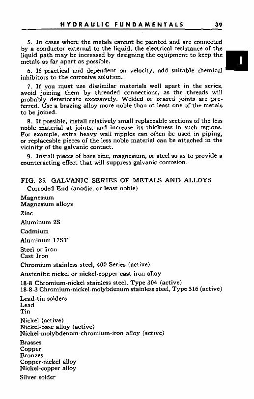
H Y D R A U L I C F U N D A M E N T A L S 39
5. In cases where the metals cannot be painted and are connected by a conductor external to the liquid, the electrical resistance of the liquid path may be increased by designing the equipment to keep the metals as far apart as possible.
6. I f practical and dependent on velocity, add suitable chemical inhibitors to the corrosive solution.
7. If you must use dissimilar materials well apart in the series, avoid joining them by threaded connections, as the threads will probably deteriorate excessively. Welded or brazed joints are pre- ferred. Use a brazing alloy more noble than at least one of the metals to be joined.
8. If possible, install relatively small replaceable sections of the less noble material at joints, and increase its thickness in such regions. For example, extra heavy wall nipples can often be used in piping, or replaceable pieces of the less noble material can be attached in the vicinity of the galvanic contact.
9. Install pieces of bare zinc, magnesium, or steel so as to provide a counteracting effect that will suppress galvanic corrosion.
U
FIG. 25. GALVANIC SERIES OF METALS AND .ALLOYS
Magnesium Magnesium alloys Zinc Aluminum 2s Cadmium Aluminum 17ST Steel or Iron Cast Iron Chromium stainless steel, 400 Series (active) Austenitic nickel or nickel-copper cast iron alloy 18-8 Chromium-nickel stainless steel, Type 304 (active) 18-8-3 Chromium-nickel-molybdenum stainless steel, Type 316 (active) Lead-tin solders Lead Tin Nickel (active) Nickel-base alloy (active) Nickel-molybdenum-chromium-iron alloy (active) Brasses Copper Bronzes Copper-nickel alloy Nickel-copper alloy Silver solder
Corroded End (anodic, or least noble)
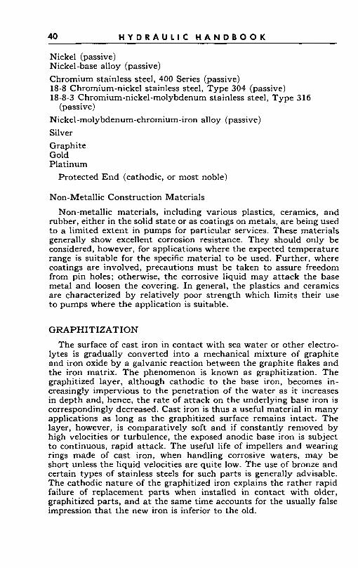
40 H Y D R A U L I C H A N D B O O K
Nickel (passive) Nickel-base alloy (passive) Chromium stainless steel, 400 Series (passive) 18-8 Chromium-nickel stainless steel, Type 304 (passive) 18-8-3 Chromium-nickel-molybdenum stainless steel, Type 316
Nickel-molybdenum-chromium-iron alloy (passive) Silver Graphite Gold Platinum
(passive)
Protected End (cathodic, or most noble)
Non-Metallic Construction Materials Non-metallic materials, including various plastics, ceramics, and
rubber, either in the solid state or as coatings on metals, are being used to a limited extent in pumps for particular services. These materials generally show excellent corrosion resistance. They should only be considered, however, for applications where the expected temperature range is suitable for the specific material to be used. Further, where coatings are involved, precautions must be taken to assure freedom from pin holes; otherwise, the corrosive liquid may attack the base metal and loosen the covering. In general, the plastics and ceramics are characterized by relatively poor strength which limits their use to pumps where the application -is suitable.
GRAPHITIZATION
The surface of cast iron in contact with sea water or other electro- lytes is gradually converted into a mechanical mixture of graphite and iron oxide by a galvanic reaction between the graphite flakes and the iron matrix. The phenomenon is known as graphitization. The graphitized layer, although cathodic to the base iron, becomes in- creasingly impervious to the penetration of the water as i t increases in depth and, hence, the rate of attack on the underlying base iron is correspondingly decreased. Cast iron is thus a useful material in many applications as long as the graphitized surface remains intact. The layer, however, is comparatively soft and if constantly removed by high velocities or turbulence, the exposed anodic base iron is subject to continuous, rapid attack. The useful life of impellers and wearing rings made of cast iron, when handling corrosive waters, may be short unless the liquid velocities are quite low. The use of bronze and certain types of stainless steels for such parts is generally advisable. The cathodic nature of the graphitized iron explains the rather rapid failure of replacement parts when installed in contact with older, graphitized parts, and a t the same time accounts for the usually false impression that the new iron is inferior to the old.
P I P E F R I C T I O N - W A T E R 41
SECTION 11-PIPE FRICTION-WATER
CONTENTS
Page Friction of Water-General ..... . . _ _ .___. ... . .......... ..... . _......___...__ ___. ... . . .. . . .... .. . . -42 Friction Tables-Schedule 40 Steel Pipe ............................................... 43 Friction Tables-Asphalt Dipped Cast Iron Pipe _..__.____________................ 52
Friction Loss in Pipe Fittings .................................................................... 58
Friction Loss-Roughness Factors ... ... ... . . ... . _ _ _ _ _ _ _ ... . . __. _ _ _ _ _ ... .. _ _ __. _.__ ........ ..62 Friction Loss-Aging of Pipe ... .. . ... . ..................... .. .. ........_____... ...... . .________ 63
. .
Friction Loss-Flexible Plastic Pipe ......... ~ ............................................ 247
42 H Y D R A U L I C H A N D B O O K
SECTION 11-FRICTION O F WATER
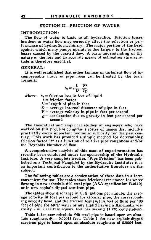
INTRODUCTION: The flow of water is basic to all hydraulics. Friction losses
incident to water flow may seriously affect the selection or per- formance of hydraulic machinery. The major portion of the head against which many pumps operate is due largely to the friction losses caused by the created flow. A basic understanding of the nature of the loss and an accurate means of estimating its magni- tude is therefore essential.
GENERAL: I t is well established that either laminar or turbulent flow of in-
compressible fluids in pipe lines can be treated by the basic formula :
L V’ h - f - - I- D 2g
where: hr = friction loss in feet of liquid. f = friction factor L = length of pipe in feet D = average internal diameter of pipe in feet V = average velocity in pipe in feet per second g = acceleration due to gravity in feet per second per
The theoretical and empirical studies of engineers who have worked on this problem comprise a roster of names that includes practically every important hydraulic authority for the past cen- tury. This work has provided a simple method for determining friction factor “f” as a function of relative pipe roughness and/or the Reynolds Number of flow.
A comprehensive anaylsis of this mass of experimentation has recently been conducted under the sponsorship of the Hydraulic Institute. A very complete treatise, “Pipe Friction” has been pub- lished as a Technical Pamphlet by the Hydraulic Institute ; it is an important contribution to the authoritative literature on the subject.
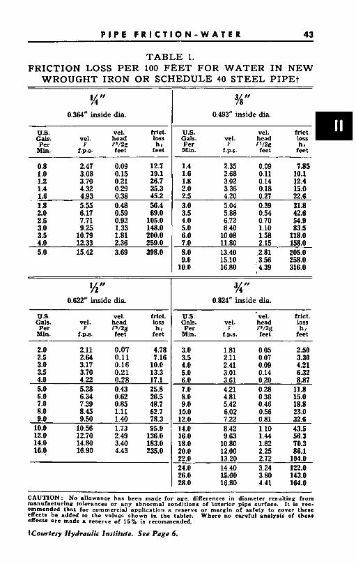
The following tables are a condensation of these data in a form convenient for use. The tables show frictional resistance for water flowing in new schedule #40 steel pipe (ASA specification B36.10) or in new asphalt-dipped cast-iron pipe.
The tkbles show discharge in U. S. gallons per minute, the aver- age velocity in feet per second for circular pipe, the correspond- ing velocity head, and the friction loss (hr) in feet of fluid per 100 feet of pipe for 60°F water or any liquid having a Kinematic vis- cosity v = 0.00001216 square feet per second (1.130 centistokes).
Table 1. for new schedule #40 steel pipe is based upon an abso- lute roughness E = 0.00015 feet. Table 2. for new asphalt-dipped cast-iron pipe is based upon an absolute roughness of 0.0004 feet.
second
P I P E F R I C T I O N - W A T E R 43
T A B L E 1. FRICTION LOSS PER 100 FEET FOR W A T E R I N N E W
WROUGHT IRON O R SCHEDULE 40 STEEL PIPEt
?4 0.364" inside &a.
U.S. vel. met. Gals. vel. head loss Per V P / 2 g h i
Mill. f.ps. feet feet
0.8 2.47 0.09 12.7 1.0 3.08 0.15 19.1 1.2 3.70 0.21 26.7 1.4 4.32 0.29 35.3 1.6 4.93 0.38 45.2 1.8 5.55 0.48 56.4 2.0 6.17 0.59 69.0 2.5 7.71 0.92 105.0 3.0 9.25 1.33 148.0 3.5 10.79 1.81 200.0 4.0 12.33 2.36 259.0 5.0 15.42 3.69 398.0
l/t " 0.622" inside dia.
us. vel. met . Gals. vel. head loss Per Y P / 2 g h i
Mln. f.ps. feet feet
2.0 2.5 3.0 3.5 4.0 5.0 6.0 7.0 8.0 9.0
10.0 12.0 14.0 16.0
2.11 0.07 2.G 0.11 3.17 0.16 3.70 0.21 4.22 0.28 5.28 0.43 6.34 0.62 7.39 0.85 8.45 1.11 9.50 1.40
10.56 1.73 12.70 2.49 14.80 3.40 16.90 4.43
4.78 7.16
10.0 13.3 17.1 25.8 36.5 48.7 62.7 78.3 95.9
136.0 183.0 235.0
0.493" inside dia.
U.S. vel. frict. Gals. vel. head loss Per I' 1"/2g h i Min. f.p.s. feet feet
1.4 1.6 1.8 2.0 2.5 3.0 3.5 4.0 5.0 6.0 7.0 8.0 9.0
10.0
2.35 0.09 2.68 o.ii 3.02 0.14 3.36 0.18 4.20 0.27 5.04 0.39 5.88 0.54 6.72 0.70 8.40 1.10
10.08 1.58 11.80 2.15 13.40 :2.81 15.10 .3.56 16.80 ' 4.39
7.85 10.1 12.4 15.0 22.6 31.8 42.6 54.9 83.5
118.0 158.0 205.0 258.0 316.0
J/r " 0.824" inside dia.
us. vel. m e t . Gals. vel. head loss Per I' 1"/2g h i Min. f.ps. feet feet
3.0 1.81 0.05 2.50 3.5 2.11 0.07 3.30 4.0 2.41 0.09 4.21 5.0 3.01 0.14 6.32 6.0 3.61 0.20 8.87 7.0 4.21 0.28 11.8 8.0 4.81 0.36 15.0 9.0 5.42 0.46 18.8
10.0 6.02 0.56 23.0 12.0 7.22 0.81 32.6 14.0 8.42 1.10 43.5 16.0 9.63 1.44 56.3 18.0 10.80 1.82 70.3 20.0 12.00 2.25 86.1 22.0 13.20 2.72 104.0 24.0 14.40 3.24 122.0 26.0 Ut30 3.80 143.0 28.0 16.80 4.41 164.0
CAUTION: No allowance has been made for age. differences in diameter resulting from manufacturing tolerances or any abnormal conditions of 'interior pipe surface. I t is rec- ommended that for commercial application a reserve or margin of safety to cover these effects be added to the values shown in the tables. Where no careful analysis of these effects are made a reserve of 15% is recommended.
tcovrtesy Hydraulic Institute. See Page 6.
44 H Y D R A U L I C H A N D B O O K
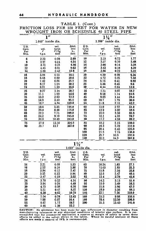
T A B L E 1. (Cont.) FRICTION LOSS P E R 100 F
WROUGHT IRON OR SC 1”
1.049” inside dia. U.S. vel. frict. Gals. vel. head loss Per Y 1”/2g ht Min. f.p.s. feet feet
6 2.23 0.08 2.68 8 2.97 0.14 4.54
10 3.71 0.21 6.86 12 4.45 0.31 9.62 14 5.20 0.42 12.8 16 5.94 0.55 16.5 18 6.68 0.69 20.6 20 7.42 0.86 25.1 22 8.17 1.04 30.2 24 8.91 1.23 35.6 25 9.27 1.34 38.7 30 11.1 1.93 54.6 35 13.0 2.63 73.3 40 14.8 3.43 95.0 45 16.7 4.34 119.0 50 18.6 5.35 146.0 55 20.4 6.46 176.0 60 22.3 7.71 209.0 65 2 4 2 9.10 245.0 70 26.0 10.49 283.0 75 27.9 12.10 324.0 80 29.7 13.7 367.0
<ET FOR WATER IN NEW IEDULE 40 S T E E L PIPE
1%’’ 1.380” inside dia.
U.S. vel. frict. Gals. vel. head loss Per Y 1”/2g ht
Min. f.p.s. feet feet
10 2.15 0.72 1.77 12 2.57 0.10 2.48 14 3.00 0.14 3.28 16 3.43 0.18 4 3 0 18 3.86 0.23 5.22 20 4.29 0.29 6.34 22 4.72 0.35 7.58 24 5.15 0.41 8.92 25 5.36 0.45 9.6 30 6.44 0.64 13.6 35 7.51 0.87 18.2 40 8.58 1.14 23.5 45 9.65 1.44 29.4 50 10.7 1.79 36.0 55 11.8 2.16 43.2 60 12.9 2.57 51.0 65 13.9 3.02 59.6 70 15.0 3.50 68.8 75 16.1 4.03 78.7 80 17.2 4.58 89.2 85 18.2 5.15 100.0 90 19.3 5.79 112.0 95 20.4 6.45 125.0
100 21.5 7.15 138.0 120 25.7 10.3 197.0 140 30.0 14.0 267.0
1 l /Lf ‘ 1.610” inside dia.
U S . dais. vel. Per Y Min. f.D.S.
14 2.21 16 2.52 18 2.84 20 3.15 22 ,3.47 24 3.78
vel. frict. head loss Y’/2g ht feet feet
0.08 1.53 0.10 1.96 0.12 2.42 0.15 2.94 0.19 3.52 0.22 4.14
25 3.94 0.24 4.48 30 4.73 0.38 6.26 35 5.51 0.47 8.37 40 6.30 0.62 10.79 45 7.04 0.78 13.45
us. vel. Met. Gals. vel. head loss
hr feet feet
Per Y Min. f.D.S.
65 10.24 1.63 70 11.03 1.89 75 11.8 2.16 80 12.6 2.47 85 13.4 2.79 90 14.2 3.13 95 15.0 3.49
100 15.8 3.86 120 18.9 5.56 140 22.1 7.56 160 25.2 9.88 180 28.4 12.50 200 31.5 15.40
27.1 31.3 35.8 40.5 45.6 51.0 56.5 62.2 88.3
119.0 156.0 196.0 241.0
50 7.88 0.97 16.4 55 8.67 1.17 19.7 60 9.46 1.39 23.2
CAUTlON: No allowance has been made for age, differences in diameter resulting from manufacturing tolerances or any abnormal conditions of interior pipe surface. It is rec- ommended that for commercial application a reserve or margin of safety to cover these effects be added to the values shown in the tables. Where no careful analysis of these effects are made a reserve of 16% is recommended.
P I P E F R I C T I O N - W A T E R 45
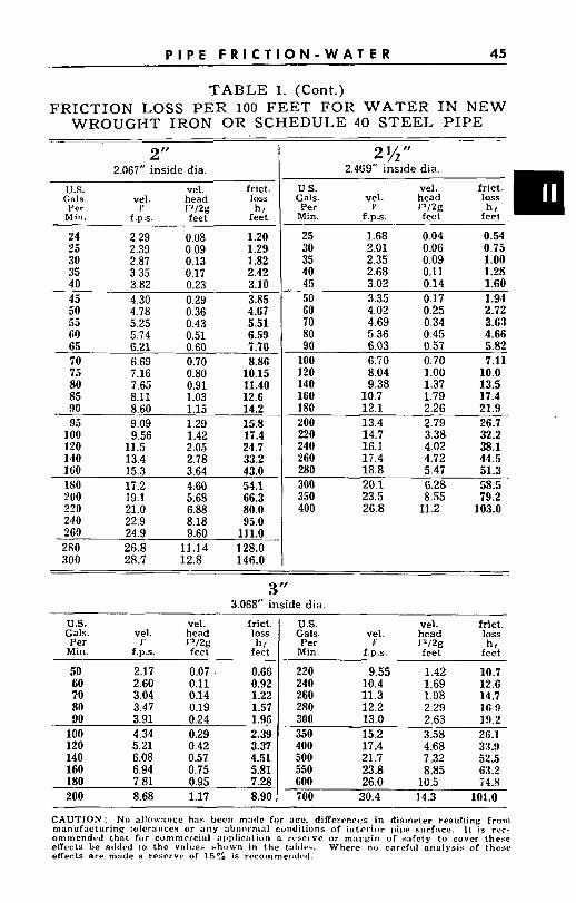
T A B L E 1. (Cont.) FRICTION LOSS P E R 100 FEET FOR W A T E R I N NEW
WROUGHT IRON O R SCHEDULE 4 0 STEEL PIPE
50 2.17 0.07 . 0.66 60 2.60 0.11 0.92 70 3.04 0.14 1.22 80 3.47 0.19 1.57 90 3.91 0.24 1.9G 100 4.34 0.29 2.39 120 5.21 0.42 3.37 140 6.08 0.57 4.51 160 6.94 0.75 5.81 180 7.81 0.95 7.28 200 8.68 1.17 8.90
2 tt 2.067” inside dia.
U.S. vel. frict. Gals. vel. head loss
I’er I‘ 11/2g hr Min. f.0.s. feet feet
220 9.55 1.42 10.7 240 10.4 1.69 12.6 260 11.3 1.98 14.7 280 12.2 2.29 11; 9 300 13.0 2.63 19.2 350 15.2 3.58 26.1 400 17.4 4.68 33.9 500 21.7 7.32 52.5 550 23.8 8.85 63.2 600 26.0 10.5 74.8 700 30.4 14.3 101.0
24 2.29 0.08 1.20 25 2.39 0.09 1.29 30 2.87 0.13 1.82 35 3.35 0.17 2.42 40 3.82 0.23 3.10 45 4.30 0.29 3.85 50 55 60 65 70
4.78 0.36 4.67 5.25 0.43 5.51 5.74 0.51 6.59 6.21 0.60 7.70 6.69 0.70 8.86
75 7.16 0.80 10.15 80 7.65 0.91 11.40
1.03 12.6
95 9.09 1.29 15.8 100 9.56 1.42 17.4 120 11.5 2.05 24.7 140 13.4 2.78 33.2 160 15.3 3.64 43.0 180 17.2 4.60 54.1 200 19.1 5.68 66.3 220 21.0 6.88 80.0 240 22.9 8.18 95.0 2GO 24.9 9.60 111.0 280 26.8 11.14 128.0 300 28.7 12.8 146.0
2 ,/” 2.469” inside dia.
frict. loss
u s. vel. Gals. vel . head Per V P/2g ht
Min. f.p.s. feet feet
25 1.68 0.04 0.54 30 2.01 0.06 0.75 35 2.35 0.09 1.00 40 2.68 n.ii 1.28 ~~ ~. ~ .. . ~~
45 3 02 0.14 1.60 50 3.35 0.17 1.94 GO 4 02 0.25 2.72 70 4.69 0.34 3.63 80 5.36 0.45 4.66 90 6 03 0 57 5.82 100 6.70 0 70 7.11 120 8 04 100 10.0 140 9 38 1.37 13.5 160 10.7 1.79 17.4 180 12.1 2.26 21.9 200 13.4 2.79 26.7 220 14.7 3.38 32.2 240 16.1 4.02 38.1 260 17.4 4.72 44.5 280 18.8 5.47 51.3 ~~
300 20.1 6.28 58.5 350 23.5 8.55 79.2 400 26.8 11.2 103.0
3 It 3.068” inside dia.
U.S. vel. vel . frict. vel. head loss
Y P / 2 g hr f.0.S. feet feet
Gals. vel. head Per I ’ P/2g
Min. f.p.s. feet
CAUTION: No allowance has becn made fc?r ace. differcnccs in diameter resulting from manufacturing tolerances or any abnornlal conditions of interittr iiiiir surface. It is rrc- ommended that for commercial api31ic:ttitin a rvscrve or mat-zin of safety to .cover there effects be added tu the values rhuwn in the kililes. Where no cnrcful analysis of these effects are made a reserve of 1596 is reconimet~ded.
46 H Y D R A U L I C H A N D B O O K
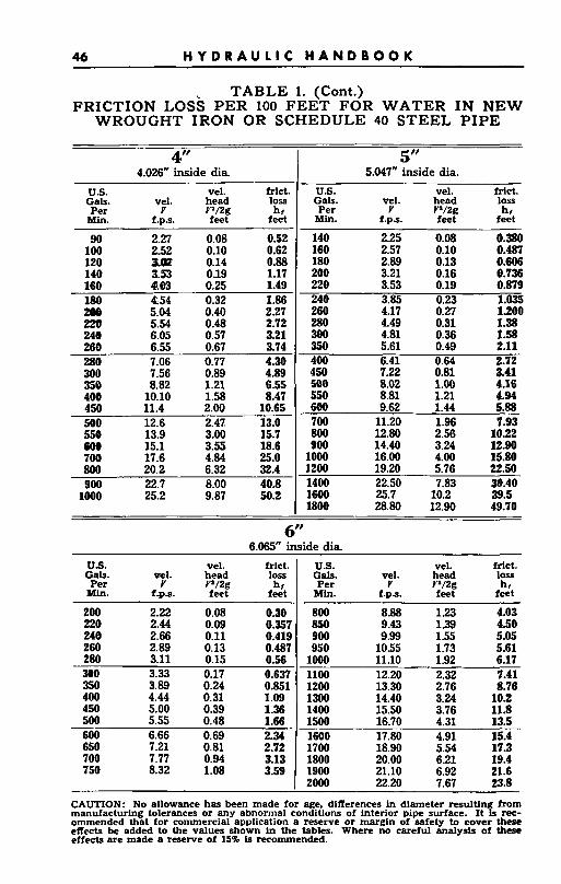
TABLE 1. (Cont.) FRICTION LOSS PER 100 FEET FOR WATER I N NEW
WROUGHT IRON OR SCHEDULE 40 STEEL PIPE
5"
2.22 0.08 0.30 2.44 0.09 0.357 2.66 0.11 0.419 2.89 0.13 0.487
4.026" inside dia us. vel. frlct. Gals. vel. head loss Per Y P / 2 g hr
Min. f.p.s. feet feet
800 8.88 123 4.03 850 9.43 139 450 900 9.99 1.55 5.05 950 10.55 1.73 5.61
90 2.27 0.08 0.52 100 252 0.10 0.62 120 Xa! 0.14 0.88 140 3.53 0.19 1.17 160 483 0.25 1.49 180 454 0.32 1.86 ZOQ 5.04 0.40 2.27 220 5.54 0.48 2.72 240 6.05 0.57 3.21 260 6.55 0.67 3.74 280 7.06 0.77 4.30 300 7.56 0.89 4.89 350 8.82 1.21 6.55 400 10.10 1.58 8.47 450 11.4 2.00 10.65 500 12.6 2.47. 13.0 550 13.9 3.00 15.7 coo 15.1 3.55 18.6 700 17.6 4.84 25.0 800 20.2 6.32 32.4 900 22.7 8.00 40.8 1000 25.2 9.87 50.2
280 3.11 0.15 0.56 300 3.33 0.17 0.637 350 3.89 0.24 0.851 400 4.44 0.31 1.09 450 5.00 0.39 1.36 - 500 5.55 0.48 1.66 600 6.66 0.69 2.34 650 7.21 0.81 2.72 700 7.77 0.94 3.13 750 8.32 1.08 3.59
5.047" inside dia. US. vel. m e t . Gals. vel. head loss Per Y v=/2g h r
Min. !.pa. feet feet
lo00 11.10 1.92 6.17 1100 12.20 2.32 7.41 1200 13.30 2.76 8.76 1300 14.40 3.24 10.2 1400 15.50 3.76 11.8 1500 16.70 4.31 13.5 1600 17.80 4.91 15.4 1700 18.90 5.54 17.3 1800 20.00 6.21 19.4 1900 21.10 6.92 21.6
140 2 160 2 180 2 200 3 220 3 240 3 260 4 280 4. 300 4 350 5 400 6. 450 7.
25 .57 .89 .21 .53 .85 .17 .49 .81 .61 41 22
0.08 0.10 0.13 0.16 0.19 0.23 0.27 0.31 0.36 0.49 0.64 0.81
0.380 0.487 0.606 0.736 0.879 1.035 1.200 1.38 1.58 2.11 2.72 3.41
c_
- 500 8.02 1.00 4.16 550 8.81 1.21 4.94 600 9.62 1.44 5.88 700 11.20 1.96 7.93 800 12.80 2.56 10.22 900 14.40 3.24 12.90 1000 16.00 4.00 15.80 1200 19.20 5.76 22.50 1400 22.50 7.83 30.40 1600 25.7 102 39.5 1800 28.80 12.90 49.70
t ' 6.065" inside dia.
us. vel. frict. U.S. vel. m e t . Gals. eel. head loss I Gals. vel. head loss Per Y W 2 g h f Per Y Y" hr
Min. fma. feet feet Min. f.DS. feet feet
I 2000 22.20 7.67 23.8 CAUTION: No allowance has been made for e. differences In diameter resulti from manufacturing tolerances or any abnormal co%itions of Interior pipe surface. It% rec- ommended that for commercial application a reserve or margin of safety to cover these effects be added to the values shown in the tables. Where no careful finalysis of these effects are made a reserve of 15% is recommended.
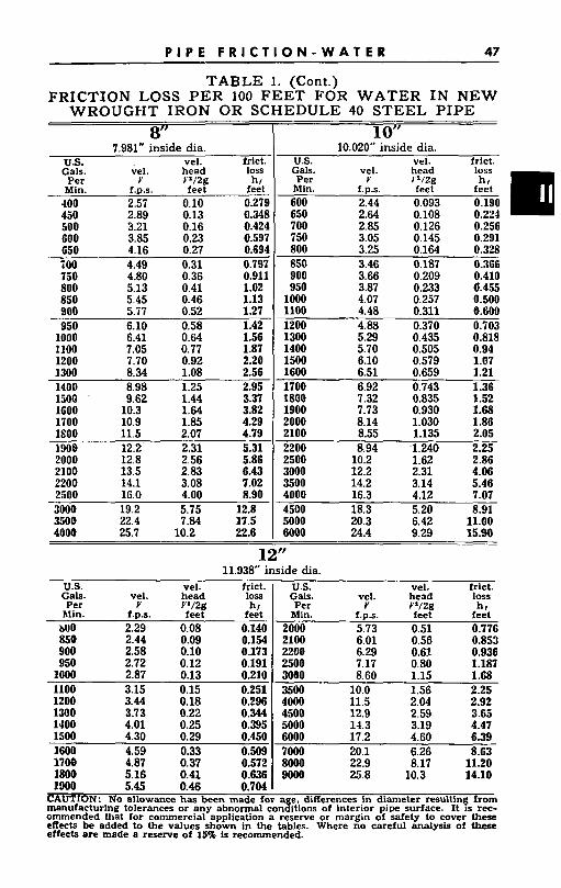
P I P E F R I C T I O N - W A T E R 47
T A B L E 1. (Cont.) FRICTION LOSS P E R 100 FEET FOR W A T E R I N N E W
W R O U G H T I R O N O R SCHEDULE 40 STEEL PIPE
US. vel. frict. Gals. vel. head loss Per Y Y'/2g ht
Min. f.ps. feet feet bUO 2.29 0.08 0.140 850 2.44 0.09 0.154 900 2.58 0.10 0.173 950 2.72 0.12 0.191 1000 2.87 0.13 0.210 1100 3.15 0.15 0.251 1200 3.44 0.18 0.296 1300 3.73 0.22 0.344 1400 4.01 0.25 0.395 1500 4.30 0.29 0.450 1600 4.59 0.33 0.509 1700 4.87 0.37 0.572 1800 5.16 0.42 0.636 1900 5.45 0.46 0.704
7.981" inside dia. U.S. vel. frict. Gals. vel. head loss
Per Y P / Z E hi
US. vel. frict. Gals. vel. head loss Per Y r=/2g ht
Min. f.p.s. feet feet 2000 5.73 0.51 0.776 2100 6.01 0.56 0.853 2200 6.29 0.61 0.936 2500 7.17 0.80 1.187 3000 8.60 1.15 1.68 3500 10.0 1.56 2.25 4000 11.5 2.04 2.92 4500 12.9 2.59 3.65 5000 11.3 3.19 4.47 6000 17.2 4.60 6.39 7000 20.1 6.26 8.63 8000 22.9 8.17 11.20 9000 25.8 10.3 14-10
~ ~~
Min. f.p.s. f e e i feet 400 2.57 0.10 0.279 450 2.89 0.13 0.348 500 3.21 0.16 0.424 GOO 3.85 0.23 0.597 C50 4.16 0.27 0.694 io0 4.49 0.31 0.797 750 4.80 0.36 0.911 800 5.13 0.41 1.02 850 5.45 0.46 1.13 900 5.77 0.52 1.27 950 6.10 0.58 1.42 1000 6.41 0.64 1.56 1100 7.05 0.77 1.87 1200 7.70 0.92 2.20 1300 8.34 1.08 2.56 1400 8.98 1.25 2.95 1500 ' 9.62 1.44 3.37 lGO0 10.3 1.64 3.82 1700 10.9 1.85 4.29 lS00 11.5 2.07 4.79 1900 12.2- 2.31 5.31 2000 12.8 2.56 5.86 2100 13.5 2.83 6.43 2200 14.1 3.08 7.02 2500 16.0 4.00 8.90 3000 19.2 5.75 12.8 3500 22.4 7 .ti4 17.5 4000 25.7 10.2 22.6
-
10.020" inside dia. U.S. vel. frict. .~ . .. ~ ~. Gals. vel. head loss Per Y P / 2 g hr
Min. f.p.s. feet feet 600 2.44 0.093 0.190 ~ .. . .._ ~ -..
650 2.64 0.108 0.221 700 2.85 0.126 0.256 750 3.05 0.145 0.291 800 3.25 0.164 0.328 850 3.46 0.187 0.366 900 3.66 0.209 0.410 950 3.87 0.233 (1.455 1000 4.07 0.257 0.500 1100 4.48 0.311 0.600 1200 4.88 0.370 0.703 1300 5.29 0.435 0.818 1400 5.70 0.505 0.94 1500 6.10 0.579 1.07 1600 6.51 0.659 1.21 1700 6.92 0.743 1.36 1800 7.32 0.835 1.52 1900 7.73 0.930 1.68 2000 8.14 1.030 1.86 2100 8.55 1.135 2.05 2200 8.94 -1.240 2.25 2500 10.2 1.62 2.86 3000 12.2 2.31 4.06 3500 14.2 3.14 5 4 6 _ _ ~. ~
4000 16.3 4.12 7.07 4500 18.3 5.20 8.91 5000 20.3 6.42 11.00 6000 24.4 9.29 15.90
48 H Y D R A U L I C H A N D B O O K
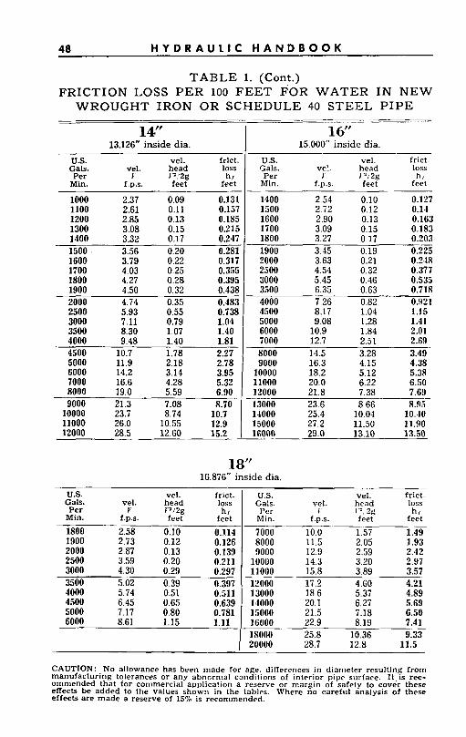
T A B L E 1. (Cont.) FRICTION LOSS P E R 100 FEET FOR W A T E R I N N E W
WROUGHT IRON OR SCHEDULE 40 S T E E L PIPE
14" 13.126" inside dia.
us. vel. frict. Gals. vel. head loss Per J i"12g h /
Min. f.P.S. feet feet ~
1000 2.37 0.09 0.131 1100 2.61 0.11 0.157 1200 2.85 0.13 0.185 1300 3.08 0.15 0.215 1400 3.32 0.17 0.247 1500 3.56 0.20 0.281 1600 3.79 0.22 0.317 1700 4.03 0.25 0.355 1800 4.27 0.28 0.395 1900 4.50 0.32 0.438 2000 4.74 0.35 0.483 2500 5.93 0.55 0.738 3000 7.11 0.79 1.04 3500 8.30 1.07 1.40 4000 9.48 1.40 1.81 4500 10.7 1.78 2.27 5000 11.9 2.18 2.78 6000 14.2 3.14 3.95 7000 16.6 4.28 5.32 8000 19.0 5.59 6.90 9000 21.3 7.08 8.70 10000 23.7 8.74 10.7 11000 26.0 10.55 12.9 12000 28.5 12.60 15.2
________ .~ ....
1 6" 15.000" inside dia.
us. vel. frict. Gals. vc!. head loss Per I' 1'*;2g h i
Min. f.p.s. feet feet
1400 2.54 0.10 0.127 1500 2.72 0.12 0.14 1600 2.90 0.13 0.163 1700 3.09 0.15 0.183
0.203 1800 3.27 0.17 1900 3.45 0.19 0.225 2000 3.63 0.21 0.248 2500 4.54 0.32 0.377 3000 5.45 n 46 0.535
-
~ ~. .. .- ~ . .~ ~~~.
3500 6.35 0.63 0.718 4000 7.26 0.82 0.!121 4500 8.17 1.03 1.15 5000 9.08 1.28 1.41 6000 10.9 1.84 2.01 sono 12.7 2.51 2.69 8000 14.5 3.28 3.49 9000 16.3 4.15 4.38
10000 18.2 5.12 5.38 11000 20.0 6.22 6.50 13000 21.8 7.38 7.69 13000 23.6 8.66 8.95- 14000 25.4 10.04 10.40 15000 27.2 11.50 11 .go 16000 29.0 13.10 13.50
18" 16.876" inside dia.
us. Gals. vel. Per Y
Min. f.p.s.
1800 2.58 1900 2.73 2000 2.87
~ . - 0.10 0.12
2500 3.59 0.20 3000 4.30 0.29 3500 5.02 0.39 4000 5.74 0.51 4500 6.45 0.65
vel. frict. loss
I ' ::a: -6 h i vel.
f.p.s. feet feet
10.0 1.57 1.49 11.5 2.05 1.93 12.9 2.59 2.42 14.3 3.20 2.97 15.8 3.89 3.57 17.3- 4.60 4.21 18.6 5.37 4.89 20.1 6.27 5.69
___-
5000 7.17 0.80 0.781 15000 21.5 7.18 6.50 6000 8.61 1.15 1.11 16000 28.7 22.9 8.19 7.41
18000 25.8 10.36 9.33 20000 12.8 11.5
CAUTION: No allowance has been made for age. differences in diameter resulting from manufacturing tolerances or any abncrnial conditions of interior pipe surface. It . is rec- ommended that for commercial application a reserve or margin of safety to cover these effects be added to the values shown in the tables. Where no careful analysis of these effects are made a reserve of 15% is recommended.
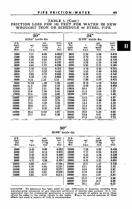
P I P E F R I C T I O N - W A T E R 49
T A B L E 1. (Cont.) FRICTION LOSS P E R 100 FEET FOR W A T E R I N N E W
WROUGHT IRON OR SCHEDULE 40 STEEL PIPE
20” 18.814” inside dia.
U.S. vel. frict. Gals. vel. head loss Per V 1”/2g hf
Min. f.p.s. feet feet
2000 2.31 0.08 0.0812 2500 2.89 0.13 0.123 3000 3.46 0.19 0.174 3500 4.04 0.25 0.232 4000 4.62 0.33 0.298 4500 5.19 0.42 0.372 5000 5.77 0.52 0.455 6000 6.92 ~ 0.75 0.645 7000 8.08 1.01 0.862 8000 9.23 1.32 1.11 9000 10.39 1.68 1.39
10000 11.5 2.07 1.70 11000 12.7 2.51 2.05 12000 13.8 2.98 2.44 13000 15.0 3.50 2.86 14000 16.2 4.08 3.29 15000 17.3 4.65 3.75 16000 18.5 5.30 4.26 18000 20.8 6.71 5.35
6.56 20000 32.1 8.28 22000 25.4 10.02 7.91 24000 27.7 11.9 9.39
___ - . . -
24” 22.626” inside dia.
frict. loss
U.S. vel. Per Y V’/2g
Gals. vel . head hi Min. f.p.s. feet feet
3000 2.39 0.09 0.0 3500 2.79 0.12 0.0 4000 3.19 0.16 0.1 4500 3.59 0.20 0.1 5000 3.99 0.25 0.1 6000 4.79 0.36 0.2 7000 5.59 0.49 0.3 8000 6.38 0.63 0.4 9@00 7.18 0.80 0.5
10000 7.98 0.99 0.6 11000 8.78 1.20 0.8 12000 9.58 1.42 0.9 13000 10.4 1.68 1.1 14000 11.2 1.94 1.2 15000 12:O 2.24 1.4 16000 12.8 2.53 1.6 17000 13.6 2.88 1.8
70 93 20 49 81 57 43 41 51 71 10 159 2 9 8 17 8
-
-
-
18000 14.4 3.21 2.10 19000 15.2 3.59 2.33 20000 16.0 3.96 2.58 25000 20.0 6.20 4.04 30000 23.9 8.91 5.68 35000 27.9 12.20 7.73
30” 29.OOO” inside dia.
us. vel. friet. Gals. vel. head loss
Per Y P / 2 g h i Min. f.p.s. feet feet
5000 2.43 0.09 0.053 6000 2.91 0.13 0.075 7000 3.40 0.18 0.100 8000 3.89 0.24 0.129 9000 4.37 0.30 0.161
10000 4.86 0.37 0.196 iiooo 5.35 0.44 0.237 12000 5.83 0.53 0.277 13000 6.31 0.62 0.320 14000 6.80 0.72 0371
us. vel. frict. Gals. vel. head loss Per Y y = / 2 g ht Min. f.p.s. feet feet
15000 7.28 0.83 0.426 16000 7.77 0.94 0.478 17000 8.25 1.06 0.538 18000 8.74 1.19 0.598 19000 9.21 1.32 0.661 20000 9.71 1.47 0.732 25000 12.1- 2.29 1.13 30000 14.6 3.30 1.61 35000 17.0 4.49 2.17 40000 19.4 5.87 2.83 45000 21.9 7.42 3.56 50000 24.3 9.17 4.38 60000 29.1 13.2 6.23 -
CAUTION: No allowance has been made for aze, differences in diameter resulting from manufacturing tolerances or any abnormal conditions of interior pipe surface. I t is rec- ommended that for commercial application a reserve or margin of safety to cover these effects he added to the values shown in the tables. Where no careful analysis of these effects are made a reserve of 15% is recommended.
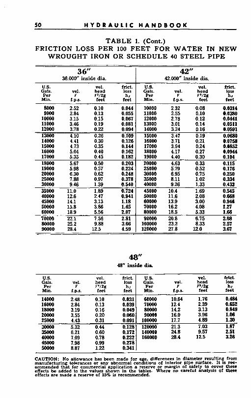
50 H Y D R A U L I C H A N D B O O K
14OOO 2.48 0.10 0.031 16OOO 2.84 0.13 0.039 MOO0 3.19 0.16 0.049 20000 3.55 0.20 0.060 25000 4.43 0.31 0.091 30000 5.32 0.44 0.128 35OOo 6.21 0.60 0.172 4OOOO 7.09 0.78 0.222 45000 7.98 0.99 0.278 5oOOo 8.87 1.22 0.341
T A B L E 1. (Cont.) FRICTION LOSS P E R 100 FEET FOR W A T E R I N N E W
WROUGHT IRON OR SCHEDULE 40 STEEL PIPE
60000 10.64 1.76 0.484 7oooO 12.4 2.39 0.652 80000 14.2 3.13 0.849 90000 16.0 3.96 1.06
1OoooO 17.7 4.89 1.30 120000 21.3 7.03 1.87 140000 24.8 9.57 2.51 16OOOO 28.4 12.5 3.26
3 6" 42" I 36.000" inside dia. 42.000'' inside dia. us. vel. met . Gals. vel. head loss Per Y YV2g h i
Min. 1.D.S. feet feet
8000 2.52 0.10 0.0 9000 2.84 0.13 0.0
10000 3.15 0.15 0.0 11000 3.46 0.19 0.0 12000 3.78 0.22 0.0 13000 4.10 0.26 0.1 14000 4.41 0.30 0.1 15000 4.73 0.35 0.1 16000 5.04 0.40 0.1 17000 5.35 0.45 0.1 18000 5.67 0.50 0.2 19000 5.98 0.57 0.2 20000 6.30 0.62 0.2 25000 7.88 0.97 0.3 30000 9.46 1.39 0.5 35000 11.0 1.89 0.7 40000 12.6 2.47 0.9 45000 14.1 3.13 1.1 50000 15.8 3.86 1.4 60000 18.9 5.56 2.0 70000 22.1 7.56 2.8 80000 25.2 9.88 3.6 90000 28.4 12.5 4.5
4
4 8 8 0 4 -
1
us. vel. frlct. Gals. vel. head 105 Per Y v=/2g hr
Min. f.D.S. feet feet
10000 2.32 0.08 0.0314 11000 2.55 0.10 0.0380 12000 2.78 0.12 0.0441 13000 3.01 0.14 0.0511 14000 3.24 0.16 0.0591 15000 3.47 0.19 0.0680 16000 3.71 0.21 0.0758 17000 3.94 0.24 0.0852 18000 4.17 0.27 0.0944 19OOO 4.40 0.30 0.104 20000 4.63 0.33 0.115 25000 5.79 0.52 0.176 30000 6.95 0.75 0.250 35000 8.11 1.02 0.334 40000 9.26 1.33 0.433 45000 10.4 1.69 0.545 50000 11.6 2.08 0.668 6oooO 13.9 3.00 0.946 70000 26.2 4.08 1.27 8OOOO 18.5 5.33 1.66 9OOOO 20.8 6.75 2.08
100000 23.2 8.33 2.57 120000 27.8 12.0 3.67
48" 48" inside dm
us. vel. frict. I US. vel. met . vel. head 105
ht f.D.0. feet p'2g feet Y
Gals. vel. head Per Y P / 2 g
Min. f.DS. feet
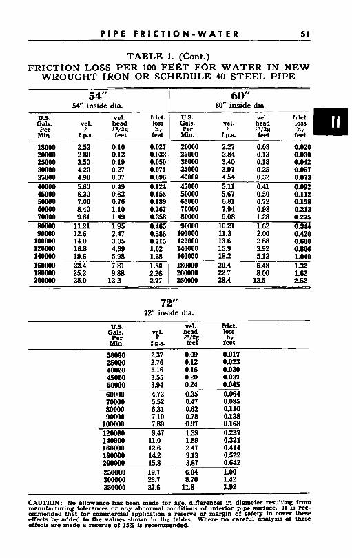
P I P E F R I C T I O N - W A T E R 51
54" inside d i a U.S. vel. met . Gals. vel. head loss Per V I =/2g h,
Min. f.p.8. feet feet
TABLE 1. (Cont.) FRICTION LOSS P E R 100 FEET FOR W A T E R I N N E W
WROUGHT IRON OR SCHEDULE 40 STEEL PIPE
54" I 60" 60" inside &a.
U.S. vel. Gals. vel. head Per Y P / 2 g ht M i . f.p.s. feet feet
30000 4.20 0.27 0.071 35000 4.90 0.37 0.096 40000 5.60 0.49 0.124
18000 2.52 0.10 0.027 20000 2.27 0.08 0.020 20000 2.80 0.12 0.0331 25000 2.84 0.13 0.030 25000 3.50 0.19 0.050 30000 3.40 0.18 0.042
35000 3.97 0.25 0.057 40000 4.54 0.32 0.073 45000 5.11 0.41 0.092
45000 6.30 0.62 0.155 50000 7.00 0.76 0.189 60000 8.40 1.10 0.267 70000 9.81 1.49 0.358 80000 11.21 1.95 0.465 90000 12.6 2.47 0.586 100000 14.0 3.05 0.715 120000 16.8 4.39 1.02 140000 19.6 5.98 1.38 160000 22.4 7.81 1.80 180000 25.2 9.88 2.26 200000 28.0 12.2 2.77
50000 5.67 0.50 0.112 60000 6.81 0.72 0.158 70000 7.94 0.98 0.213 80000 9.08 1.28 0.275 90000 10.21 1.62 0.344 100000 11.3 2.00 0.420 120000 13.6 2.88 0.600 140000 15.9 3.92 0.806 160000 18.2 5.12 1.040 180000 20.4 6.48 132 200000 22.7 8.00 1.62 250000 28.4 12.5 2.52
72" 72" inside dia.
U.S. vel. met . Gals. vel. head lOSS
V P / 2 hr Per Min. f .ps. f e e t feet
~~
3OOOO 2.37 0.09 0.017 35OOo 2.76 0.12 0.023 40000 3.16 0.16 0.030 45000 3.55 0.20 0.037 50000 3.94 0.24 0.045 6OOOO 4.73 0.35 0.064 7oooo 552 0.47 0.085 8OOOO 631 0.62 OJlO go000 7.10 0.78 0.138 1OOOOO 7.89 0.97 0.168 120000 9.47 1.39 0237 140000 11.0 1.89 0321 160000 12.6 2.47 0.414 180000 142 3.13 0522 200000 15.8 3.87 0.642 250000 19.7 6.04 1 .oo 3oO000 23.7 8.70 1.42 35o000 27.6 11.8 1.92
CAUTION: No allowance has been made for aee. dlfferenees in diameter reSdtint7 from &Guta&&ig GlerGeeS or-~~abnormaicona~tiions bf interior pipe surface. It k ree- ommended that for commercial application a reserve or margin of safety to cover the effects be added to the values shown in the tables. Where no careful aalySh Of the effects are made a reserve of 15% b recommended.
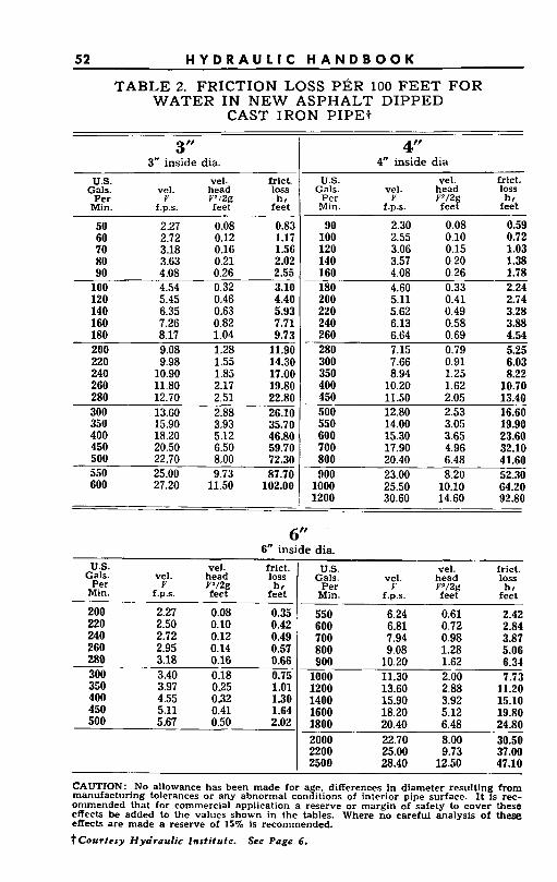
52 H Y D R A U L I C H A N D B O O K
T A B L E 2. FRICTION LOSS P E R 100 FEET F O R WATER I N N E W ASPHALT D I P P E D
CAST IRON P I P E ?
3 “ 3” inside dia.
us. vel. frict. Gals. vel. head loss
Per Y v=/2g hr Min. f.p.s. feet feet
50 2.27 0.08 0.83 60 2.72 0.12 1.17 70 3.18 0.16 1.56 80 3.63 0.21 2.02 90 4.08 0.26 2.55 100 4.54 0.32 3.10 120 5.45 0.46 4.40 140 6.35 0.63 5.93 160 7.26 0.82 7.71 180 8.17 1.04 9.73 200 9.08 1.28 11.90 220 9.98 1.55 14.30 240 10.90 1.85 17.00 260 11.80 2.17 19.80 280 12.70 2.51 22.80 300 13.60 2.88 26.10 350 15.90 3.93 35.70 400 18.20 5.12 46.80 450 20.50 6.50 59.70 500 22.70 8.00 72.30 550 25.00 9.73 87.70 600 27.20 11.50 102.00
us. vel. frict. Gals. vel. head loss Per Y P/2g h i Min. f.D.S. feet feet
~~
90 2.30 0.08 0.59 100 2.55 0.10 0.72 120 3.06 0.15 1.03 140 3.57 0.20 1.38 160 4.08 0.26 1.78 180 4.60 0.33 2.24 200 5.11 0.41 2.74 220 5.62 0.49 3.28 240 6.13 0.58 3.88 260 6.64 0.69 4.54 280 7.15 0.79 5.25 300 7.66 0.91 6.03 350 8.94 1.25 8.22 ~ ~~
400 10.20 1.62 10.70 450 11.50 2.05 13.40 500 12.80 2.53 16.60 550 14.00 3.05 19.90 600 15.30 3.65 23.60 700 17.90 4.96 32.10 800 20.40 6.48 41.60 900 23.00 8.20 52.30 1000 25.50 10.10 64.20 1200 30.60 14.60 92.80
6” 6” inside dia.
U.S. Gals.
Per Min.
200 220 240 260 280 300 350 400 450 500
vel. vel. head Y P/2g
f.u.s. feet 2.27 0.08 2.50 0.10 2.72 0.12 2.95 0.14 3.18 0.16 3.40 0.18 3.97 0.25 4.55 0.32
frict. loss hr feet
0.35 0.42 0.49 0.57 0.66 0.75 1.01 1.30
5.11 0.41 1.64 5.67 0.50 2.02
~~ ~
4” 4” inside dia
us. vel. frict. Gals. vel. head loss
Per Y Y’/2g h i Min. f.p.s. feet feet
550 600 700 Rnn -._
900 1000 1200 1400 1600 1800 2000 2200 2500
6.24 6.81 7.94 9.08 10.20 11.30 13.60 15.90 18.20 20.40 22.70 25.00 28.40
0.61 0.72 0.98 1.28 1.62 2.00 2.88 3.92 5.12 6.48 8.00 9.73 12.50
2.42 2.84 3.87 5.06 6.34 7.73 11.20 15.10 19.80 24.80 30.50 37.00 47.10
CAUTION: No allowance has been made for age differences in diameter resulting from manufacturing tolerances or any abnormal condi6ons of interior pipe surface. It is rec- ommended that for commercial application a reserve or margin of safety to cover these effects be added to the values shown in the tables. Where no careful analysis of these effects are made a reserve of 15% is recommended. tCourtery Hydraulic Institute. See Page 6.
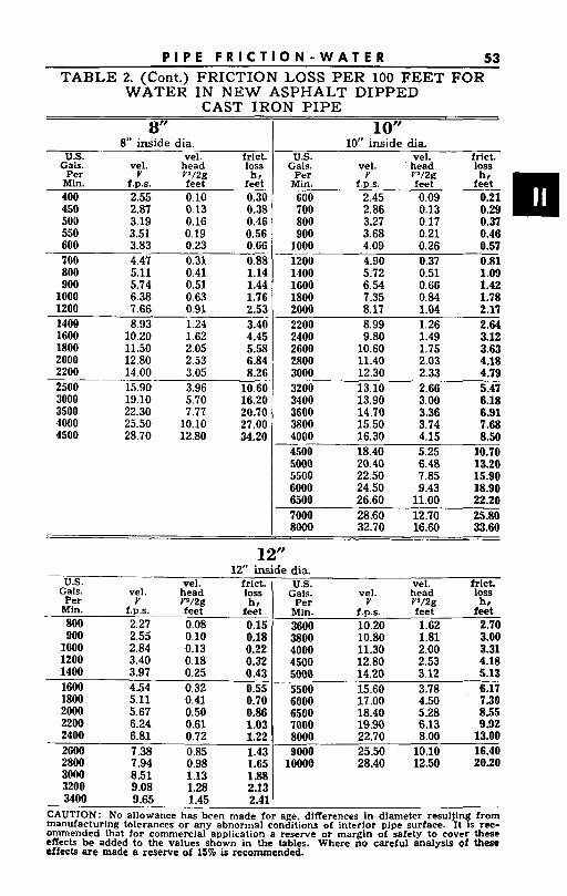
P I P E F R I C T I O N - W A T E R 53 TABLE 2. (Cont.) FRICTION LOSS PER 100 FEET FOR
WATER IN NEW ASPHALT DIPPED CAST IRON PIPE
8” I 10” frict. loss hr
feet 0.30 0.38 0.46 0.56 0.C6
~
U.S. Gals.
Per Min. 400 450
U.S. Gals.
Per Min. 600 700 800 900
1000
-.___
500 550 600 700 4.47 0.31 0.88 800 5.11 0.41 1.14 900 5.74 0.51 1.44
1000 6.38 0.63 1.76 1200 7.66 0.91 2.53 1408 8.93 1.24 3.40 1600 10.20 1.62 4.45 1800 11.50 2.05 5.58 2000 12.80 2.53 6.84 2200 14.00 3.05 8.26 2500 15.90 3.96 10.66 3000 19.10 5.70 16.20 3500 22.30 7.77 20.70 4000 25.50 10.10 27.00
28.70 12.80 34.20 4500
8“ inside dia. __- v e l .
vel. head Y Y”
f.p.s. feet 2.55 0.10
- 1200 4.90 0.37 0.81 1400 5.72 0.51 1.09 1600 6.54 0.66 1.42 1800 7.35 0.84 1.78 2000 8.17 1.04 2.11 2200 8.99 1.26 2.64 2400 9.80 1.49 3.12 2600 10.60 1.75 3.63 2800 11.40 2.03 4.18 3000 12.30 2.33 4.79 3200 13.10 2.66 5.47 3400 13.90 3.00 6.18 3600 14.70 3.36 6.91 3800 15.50 3.74 7.68 4000 16.30 4.15 8.50 4500 18.40 5.25 10.70 5000 20.40 6.48 13.20 5500 22.50 7.85 15.90 6000 24.50 9.43 18.90 6500 26.60 11.00 22.20 7000 28.60 12.70 25.80 8000 32.70 16.60 33.60
-
2.87 0.13 3.19 0.16 3.51 0.19 3.83 0.23
U.S. vel. frlct. Gals. vel. head loss
Per Y v = / 2 g hr Min. f .p.s. feet feet 800 2.27 0.08 0.15 900 2.55 0.10 0.18
1000 2.84 0.13 0.22 1200 3.40 0.18 0.32 1400 3.97 0.25 0.43 1600 4.54 0.32 0.55 1800 5.11 0.41 0.70 2000 5.67 0.50 0.86 2200 6.24 0.61 1.03 2400 6.81 0.72 1.22 2600 7.38 0.85 1.43 2800 7.94 0.98 1.65 3000 8.51 1.13 1 .UR
U.S. vel. frict. Gals. vel. head loss
Per V Y” hr Min. f .p.s. feet feet 3600 10.20 1.62 2.70 3800 10.80 1.81 3.00 4000 11.30 2.00 3.31 4500 12.80 2.53 4.18 5000 14.20 3.12 5.13 5500 15.60 3.78 6.17 6000 17.00 4.50 730 6500 18.40 5 2 8 855 7000 19.90 6.13 9 9 2 8000 22.70 8.00 13.00 9000 25.50 10.10 16.40
10000 28.40 12.50 2030
10” inside
vel. V
f.p.s. 2.45 2.86 3.27 3.68 4.09
dia. vel.
’ head 1”/2g feet 0.09 0.13 0.17 0.21 0.26
__.
frlct. loss 41kw 0.29
0.37 0.46 0.57
3200 9.08 1.28 233 I 3400 9.65 1.45 2.41
CAUTION: No allowance has been made for age differences in dlameter resultin from manufacturing tolerances or any abnormal condiiions of interior pipe surface. It ‘i, rec- ommended that for commercial application a reserve or margin of safety to cover t h e e effects be added to the values shqwn in the tables. Where no careful analysls of these Ctfects ere made 8 reserve of 15% 1s recommended.
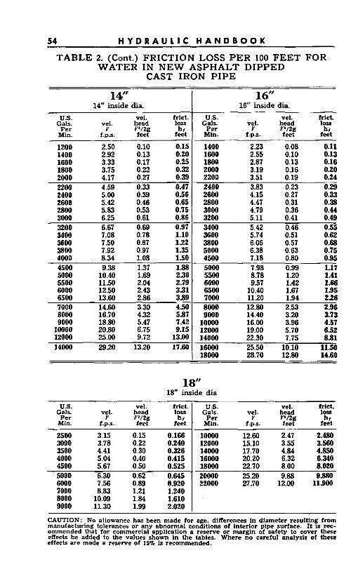
54 H Y D R A U L I C H A N D B O O K
~
14" 14" inside &a.
us. vel. frict. Gals. vel. head loss
Per Y Y'/2g h f Min. f.p.s. feet feet
1200 2.50 0.10 0.15 1400 2.92 0.13 0.20 1600 3.33 0.17 0.25 1800 3.75 0.22 0.32 2000 4.17 0.27 0.39 2200 4.59 0.33 0.47 2400 5.00 0.39 0.56 2600 5.42 0.46 0.65 2800 5.83 0.53 0.75 3000 6.25 0.61 0.86 3200 6.67 0.69 0.97 3408 7.08 0.78 1-10 3600 7.50 0.87 1.22 3800 7.92 0.97 1.35 4000 8.34 1.08 1.50 4500 9.38 137 1.88 5000 10.40 1.69 230 5500 11.50 2.04 2.79 6000 12.50 2.43 331 6500 13.60 2.86 3.89 7000 14.60 3.30 450 8000 16.70 4.32 5.87 9000 18.80 5.47 7.42
10000 20.80 6.75 9.15 12000 25.00 9.72 13.00 14000 2920 1320 17.60
TABLE 2. (Cont.) FRICTION LOSS PER 100 FEET FOR WATER IN NEW ASPHALT DIPPED
CAST IRON PIPE
1 6" 16" inside dia.
Gals. vel. head losS Per Y Y'/2 hr
Min. f.p.s. f e e t feet
1400 223 0.08 0.11 1600 2.55 0.10 0.13 1800 2.87 0.13 0.16 2000 3.19 0.16 0.20 2200 3.51 0.19 0.24 2400 3.83 0.23 0.29 2600 4.15 0.27 0.33 2800 4.47 0.31 0.38 3000 4.79 0.36 0.44 3200 5.11 0.41 0.49 3400 5.42 0.46 0.55 3600 5.74 0.51 0.62 3800 6.06 0.57 0.68 5000 6.38 0.63 0.75 4500 7.18 0.80 0.95 5000 7.98 0.99 1.17 5500 8.78 120 1.41 6000 9.57 1.42 1.66 6500 10.40 1.67 195 7000 1120 134 226 8000 12.80 2.53 2.96 9000 14.40 3.20 3.73
10000 16.00 3.96 4.57 12000 19.00 5.70 6.52 14000 22.30 7.75 8.81 16000 25.50 10.10 11.50 18000 28.70 12.80 14.60
U.S. vel. mct.
2500 3.15 0.15 0.166 3000 3.78 0.22 0.240 3500 4.41 0.30 0.326 4000 5.04 0.40 0.415 4500 5.67 0.50 0.525 5000 6.30 0.62 0.645 6000 7.56 0.89 8.920 7000 8.83 1.21 1.240 8000 10.09 1.84 1.610 9000 11.30 1.99 2.020
18" 1 8 inside dia
10000 12.60 2.47 2.480 12000 15.10 3.55 3.560 14000 17.70 4.84 4.850 16000 20.20 6.32 6.340 18000 22.70 8.00 8.020 20000 25.20 9.88 9.880 22000 27.70 12.00 11900
us. vel. frict. us. vel. mct. Gals. vel. head loss 1 Gals. vel. head 1-
Per Y Y'/2g h f Per Y Y'/2 hr Min. f.u.s. feet Zeet Min. f.D.6. f e e t feet

P I P E F R I C T I O N - W A T E R 55
TABLE 2. (Cont.) FRICTION LOSS P E R 100 FEET FOR WATER IN N E W ASPHALT DIPPED
CAST IRON PIPE
20” 20” inside dia.
U.S. vel. frict. Gals. vel. head loss P.er P Y’/2 hr
Mm. f.D.8. ieef feet ~~
2500 2.55 0.10 0.0998 3000 3.06 0.15 0.140 3500 3.57 0.20 0.188 4000 4.08 0.26 0.243 4500 4.59 0.33 0.306 5000 5.11 0.41 0.376 6000 6.13 0.58 0.533 7000 7.15 0.79 0.721 8000 8.17 1.04 9000 9.19 1.31 10000 10.20 1.62 12000 14000 16000 18000 20000 22000 24000 26000 28000 30000
12.30 2.33 14.30 3.18 16.30 4.15 18.40 5.25 20.40 6.48 22.50 7.84 24.50 9.33 26.50 10.95
30.60 14.60 28.50 12.64
0.935 1.18 1.45 2.07 2.80 3.66 4.62 5.67 6.85 8.13 9.54 11.05 12.70
24’’ ~- 24” inside &a.
U.S. vel. Gals. vel. head loss
Per Y Y’/2 hr Min. f.P.s. ieef feet
~ ~~
3500 2.48 0.10 0.0759 4000 2.84 0.13 0.098 4500 3.19 0.16 0.122 5000 3.55 0.20 0.149 6Ooo 4.26 0.28 0.211 7000 4.96 0.38 0.284 8000 5.67 0.50 0.368 9000 6.38 0.63 0.464 10000 7.09 0.78 0.571 12000 851 1.13 0.816 14OOO 9.93 1.53 1.11 16000 11.35 2.00 1.43 18000 12.76 2.53 1.80 20000 14.20 .3.13 2.21 22000 15.60 .3.78 2.67 24000 17.00 4.50 3.16 26000 18.40 5.28 3.71 243000 19.80 6.10 4.30 30000 21.30 7.03 4.97
40000 28.40 12.50 8.75 35000 24.90 9.58 6.78
3 0” 30” inside dia
U.S. vel. met. Gals. vel. head loSa
Per Y P I 2 hr Mln. f.D.S. feef feet
5000 227 0.08 0.0488 6000 2.72 0.12 0.069 7000 3.18 0.16 0.092 8000 3.63 0.21 0.119 go00 4.08 0.26 0.149 10000 4.54 0.32 0.183 12000 5.45 0.46 0.260 14000 6.35 0.63 0.351 16OOO 7.26 0.82 0.455 18000 8.17 1.04 0.572
U.S. vel. m e t Gals. vel. head loss
Per P P I 2 hr Min. f.D.S. f e e l feet
20000 9.0s 1.211 0.703 22000 10.00 155 0.856 24000 10.90 1.84 1.01 26000 11.80 2.16 1.17 28Ooo 12.70 2.50 1.34 30000 13.60 2.88 157 35Ooo 15.90 3.92 2.13 40000 1820 5.12 2.71 45000 20.40 6.48 350 50000 22.70 8.00 430 60000 27.20 11.50 619
CAUTION: No allowance has been made for age. differences In dlameter resulting from manufacturing tolerances or any abnormal conditions of interior pipe surface. It is rec- ommended that for commercial application a reserve or margin of safety to cover these effects be added b the values shown in the tables. Where no careful analysis of these effects are made a reserve of 15% is recommended.
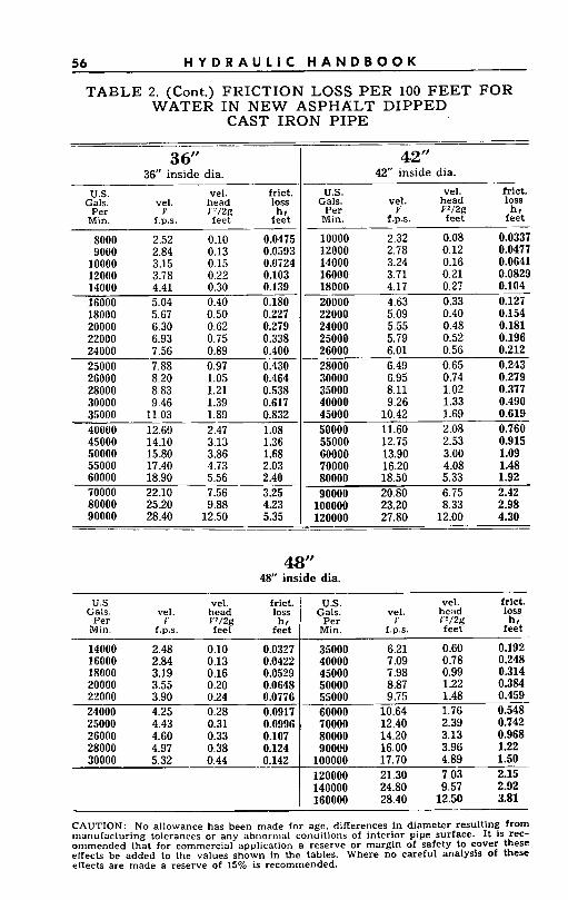
56 H Y D R A U L I C H A N D B O O K
TABLE 2. (Cont.) FRICTION LOSS P E R 100 FEET FOR WATER IN N E W ASPHALT DIPPED
CAST IRON PIPE
3 6” 36” inside dia.
~~
us. vel. frict. Gals. vel. head loss
Per Y v / 2 g hr Min. f.p.s. feet feet
8000 2.52 0.10 0.0475 9000 2.84 0.13 0.0593
10000 3.15 0.15 0.0724 12000 3.78 0.22 0.103 14000 4.41 0.30 0.139 16000 5.04 0.40 0.180 18000 5.67 0.50 0.227 20000 6.30 0.62 0.279 22000 6.93 0.75 0.338 24000 7.56 0.89 0.400 25000 7.88 0.97 0.430 26000 8.20 1.05 0.464 28000 8.83 1.21 0.538 30000 9.46 1.39 0.617 35000 11.03 1.89 0.832 40000 12.60 2.47 1.08 45000 14.10 3.13 1.36 50000 15.80 3.86 1.68 55000 17.40 4.73 2.03 60000 18.90 5.56 2.40 70000 22.10 7.56 3.25 80000 25.20 9.88 4.23 90000 28.40 12.50 5.35 _ _ _ _ _ _ _ _ ~
42 I’ 42“ inside dia.
U.S. vel. frict. Gals. vel. head loss
Per V P / 2 g ht Min. f.p.s. feet feet
10000 2.32 0.08 0.0337 I2000 2.78 0.12 0.0477 14000 3.24 0.16 0.0641 16000 3.71 0.21 0.0829 18000 4.17 0.2? 0.104 20000 4.63 0.33 0.127 22000 5.09 0.40 0.154 24000 5.55 0.48 0.181 25000 5.79 0.52 0.196 26000 6.01 0.56 0.212 28000 6.49 0.65 0.243 30000 6.95 0.74 0.279 35000 8.11 1.02 0.377 40000 9.26 1.33 0.490 45000 10.42 1.69 0.619 50000 11.60 2.08 0.760 55000 12.75 2.53 0.915 GO000 13.90 3.00 1.09 70000 16.20 4.08 1.48 80000 18.50 5.33 1.92 90000 20.80 6.75 2.42
100000 23.20 8.33 2.98 I20000 27.80 12.00 4.30
48” 48” inside dia.
us. vel. frict. Gals. vel. head loss
Per I ’ 1’*/2g hr Min. f.p.s. feet feet
U.S. vel. frict. Gals. vel. head loss
Per I’ 1”/2g hr Min. f.p.s. feet feet
14000 2.48 16000 2.84 18000 3.19 20000 3.55 2‘000 3.90 24000 4.25 25000 4.43 26000 4.60 28000 4.97 30000 5.32
0.10 0.0327 0.13 0.0422 0.16 0.0529 0.20 0.0648 0.24 0.0776 0.28 0.0917 0.31 0.0996 0.33 0.107 0.38 0.124 0.44 0.142
35000 6.21 0.60 0.192 40000 7.09 0.78 0.248 45000 7.98 0.99 0.314 50000 8.87 1.22 0.384 55000 9.75 1.48 0.459 60000 10.64 1.76 0.548- 70000 12.40 2.39 0.742 80000 14.20 3.13 0.968 90000 16.00 3.96 1.22
100000 17.70 4.89 1.50 I20000 21.30 7.03 2.15 i4oooo 24.80 9.57 2.92 I 160000 28.40 12.50 3.81
CAUTION: No allowance has been made for age, differences in diameter resulting from manufacturing tolerances or any abnormal condilions of interior pipe surface. It is ret- ommended that for commercial application a reserve or margin of safety to cover these effects be added to the values shown in the tables. Where no careful analysis Of these effects are made a reserve of 15% is recommended.
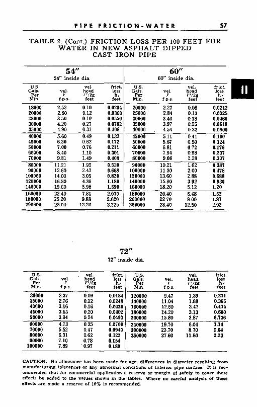
P I P E F R I C T I O N - W A T E R 57
TABLE 2. (Cont.) FRICTION LOSS PER 100 FEET FOR WATER I N N E W ASPHALT DIPPED
CAST IRON PIPE
5 4” 54” inside dia.
US. vel. frict. Gals. vel. head loss
Per I’ P / 2 g ht Min. f.p.s. feet feet 18000 2.52 0.10 20000 2.80 0.12 25000 3.50 0.19 30000 4.20 0.27 35000 4.90 0.37 40000 5.60 0.49 45000 6.30 0.62 50000 7.00 0.76 60000 8.40 1.10 70000 9.81 1.49
0.0294 0.0360 0.0550 0.0782 0.106 0.137 0.172 0.211 0.301 0.408
80000 11.21 1.95 0.530 90000 12.60 2.47 0.668
100000 14.00 3.05 0.820 120000 16.80 4.39 1.180 140000 19.60 5.98 1.590 160000 22.40 7.81 2.070 180000 25.20 9.88 2.620 200000 28.00 12.20 3.220
60” ~~
60” inside dia. us. vel. head vel. frict. loss 131
Gals. Per I I‘=/2g hr Min. f.p.s. feet feet
20000 2.27 0.08 0.0212 25000 2.84 0.13 0.0325 30000 3.40 0.18 0.0460 35000 3.97 0.25 0.0618 40000 . 4.54 0.32 0.0800 45000 5.11 0.41 0.100 50000 5.67 0.50 0.124 60000 6.81 0.72 0.176 70000 7.94 0.98 0.237 80000 9.08 1.28 0.307 90000 10.21 1.62 0.387
100000 11.30 2.00 0.478 120000 13.60 2.88 0.688 140000 15.90 3.92 0.930 160000 18.20 5.12 1.20 180000 20.40 6.48 1.52 200000 22.70 8.00 1.87 250000 28.40 12.50 2.92
12/’ 72” inside dia.
U.S. . vel. frict. Gals. vel. head loss
Per Y P / 2 g hr Min. f.p.s. feet feet
~
US. vel. frict. Gals. vel. head loss
Per I’ r=/2 ht Min. f.p.s. feek feet 30000 2.37 0.09 35000 2.76 0.12 40000 3.16 0.16 45000 3.55 0.20 50000 3.94 0.24 60000 4.73 0.35 70000 5.52 0.47 80000 6.31 0.62 90000 7.10 0.78
100000 7.89 ’ 0.97
0.0184 0.0248 0.0320 0.0402 0.0493 0.0700 0.8940 0.122 0.154 0.189
120000 9.47 140000 11.04 160000 12.60 180000 14.20 200000 15.80 250000 19.70 300000 23.70 350000 27.60
1.39 0.271 1.89 0.365 2.41 0.475 3.13 0.600 3.87 0.736 6.04 1.14 8.70 1.64
11.80 2.23
CAUTION: No allowance has been made for age. differences In diameter resultlng from manufacturing tolerances or any abnormal conditions of interior pipe surface. It Is rec- ommended that for commercial application a reserve or margln of safety to cover these effects be added to the values shown in the tables. Where no careful analysis of these effects are made a reserve of 15% is recommended.
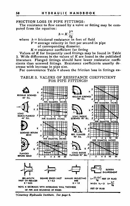
58 H Y D R A U L I C H A N D B O O K
BELLMOUTH SQUARE EDGED INLET INWARD PROJECnNG INLET OR REDUCER K = 0.5 PIPE
NOTEX K D K R W E S WITH INCREASING W A U THICKNESS
K = 0.05 K - 1.0
OF FlPE AND ROUNDING OF EDGES
FRICTION LOSS IN PIPE FITTINGS:
puted from the equation : The resistance to flow caused by a valve or fitting may be com-
V2 h = K -
2g where h = frictional resistance in feet of fluid
V = average velocity in feet per second in pipe of corresponding diameter.
K = resistance coefficient for fitting Values of K for frequently used fittings may be found in Table
3. Wide differences in the values of K are found in the published literature. Flanged fittings should have lower resistance coeffi- cients than screwed fittings. Resistance coefficients usually de- crease with increase in pipe size.
For convenience Table 4 shows the friction loss in fittings ex-
h=(VI-VI)' FEET OF FLUID
WHEN V z - 0 h - 3
FEET OF FLUID
20
20
TABLE 3. VALUES O F RESISTANCE COEFFICIENT FOR PIPE FITTINGSt
45- ELL. 9.3 .5 1 2 d +:$ K .2 .3
LONG RAMUS RANGED -1
45' ELL.
K
SCREWED RETURN BEND
PIPE DIAMETER, INCHES
2
1
.d .5 I a 4 PIPE DIAMETER, INCHES
HANGED RETURN BEND
K
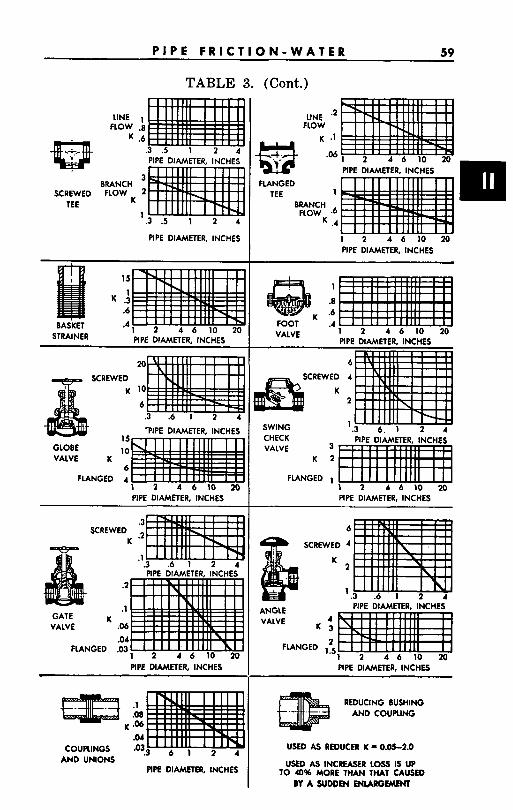
P I P E F R I C T I O N - W A T E R 59
TABLE 3. (Cont.)
SCREWED TEE
LINE FLOW
K
BRANCH FLOW
K
.8 1
.6
PIPE DIAMETER, INCHES
3 2
1 ' 3 . 5 1 2 4
PIPE DIAMETER, INCHES
PIPE DIAMETER, INCHES
FLANGED .03 1 2 4 6 10 20 PIPE DIAMETER, INCHES
COUPLINGS A N D UNIONS
K
.1
.08 , .06
.04
'0?3 6 1 2 4
APE DIAMETER. INCHES
FLANGED TEE
LINE " FLOW
K
.06
1 BRANCH
FLOW .6 K .4
PIPE DIAMETER, INCHES
1 2 4 6 1 0 20 PIPE DIAMETER, INCHES
VALVE
SWING CHECK PIPE DIAMETER. INCHES VALVE 3
K 2
FLANGED 1 1 2 4 6 1 0 20 PIPE DIAMETER, INCHES
ANGLE VALVE
FLAh
SCRE
K
lGED 1 2 4 6 10 20 PIPE DIAMETER. INCHES
REDUCING BUSHING AND COUPLING
USED AS REDUCER K 0.05-2.0
USED AS INCREASER LOSS IS UP TO 40% MORE THAN THAT CAUSED
BY A SUDDEN WuDcfMcNI
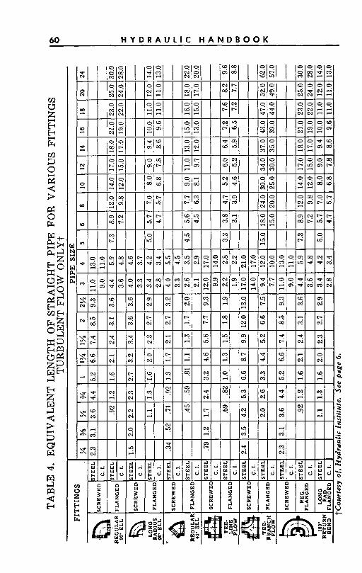
60 H Y D R A U L I C H A N D B O O K
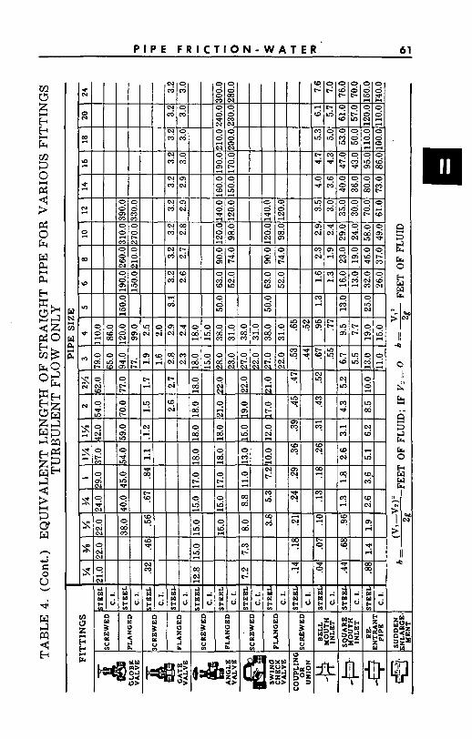
P I P E F R I C T I O N - W A T E R 61
62 H Y D R A U L I C H A N D B O O K
pressed as an equivalent length of straight pipe. This presentation is simple to use on complicated piping layouts involving an assort- ment of different fittings and is especially well suited to the prep- aration of station curves where varying rates of flow are involved.
FRICTION I N OTHER TYPES OF PIPE The preceding tabulations for friction loss in pipes apply to
new schedule #40 steel pipe and new asphalt-dipped cast-iron pipe as noted. Friction loss in other types of pipe vary from these values due to the difference in the average relative roughness of the interior surface of such pipes as commercially manufactured.
The following chart Fig. 26 shows relative roughness factors
($)for new clean pipes as commercially manufactured plotted against pipe diameter in inches. The curves for schedule #40 steel pipe (absolute roughness 0.00015’) and asphalt-dipped cast- iron pipe (absolute roughness 0.0004’) on which the previous Tables 1 and 2 are based are shown on this curve.
The ratio of the friction factor for any pipe to that for schedule #40 steel pipe may be used as a multiplier to adjust the friction losses shown in Table 1 to apply to the other type of pipe.
I t must be recognized that various types of pipe as commercially manufactured are subject to a considerable variation in roughness. Average values for good clean new pipe however yield the multi- pliers recommended in the following Table 5.
TABLE 5. MULTIPLIERS TO APPLY TO VALUES FROM TABLE 1 TO OBTAIN FRICTION LOSS IN OTHER TYPES
O F PIPE OR CONDUIT. Multiplier to
Appl to Table 1 t;a~yes
of Friction Loss Type of New Conduit or Pipe
Rubber lined hose 0.72 Spun cement line pipe 0.76 Spun bitumastic enameled pipe 0.76 Aluminum irrigation pipe 0.81
Copper or Brass pipe 0.86 Seamless steel tubing 0.86 Glass tube or pipe 0.86
1 .oo
Transite Pipe 0.85
Schedule #40 steel pipe Wood Stave pipe 1.15 Galvanized iron pipe 1.22 Vitrified pipe 1.36 Spiral riveted pipe (flow with lap) 1.40 Spiral riveted pipe (flow against lap) 1.70 Unlined linen hose 1.80
The multipliers in Table 5 provide for the difference in type of pipe only. They do not include deviations in internal diameter from schedule #40 steel pipe.
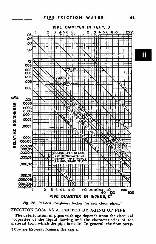
P I P E F R I C T I O N - W A T E R 63
PIPE DIAMETER I N FEET, 0
PIPE DIAMETER IN INCHES, 0” Fig. 26. Relative roughness factors for new clean pipes.+
FRICTION LOSS AS AFFECTED B Y AGING OF PIPE The deterioration of pipes with age depends upon the chemical
properties of the liquid flowing and the characteristics of the material from which the pipe is made. In general, the flow carry- t Courtesy Hydraulic Institute. See page 6.
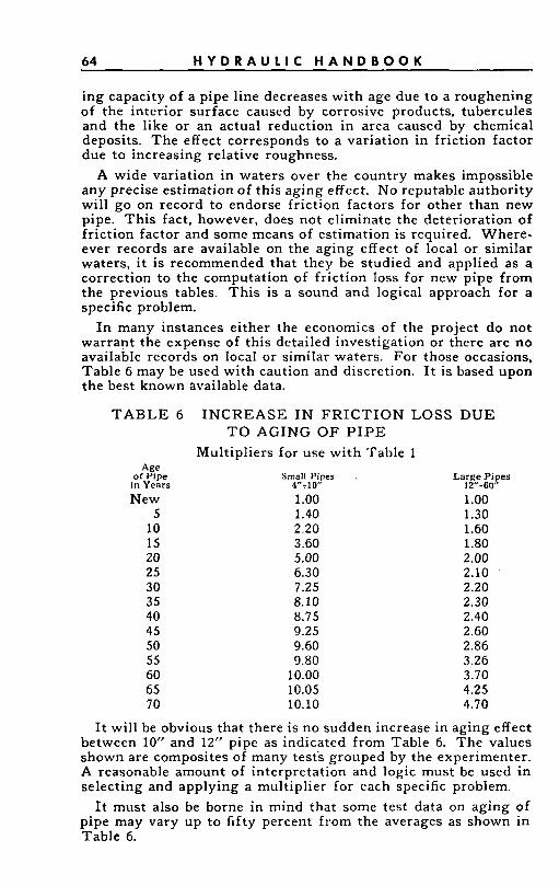
64 H Y D R A U L I C H A N D B O O K
ing capacity of a pipe line decreases with age due to a roughening of the interior surface caused by corrosive products, tubercules and the like or an actual reduction in area caused by chemical deposits. The effect corresponds to a variation in friction factor due to increasing relative roughness.
A wide variation in waters over the country makes impossible any precise estimation of this aging effect. No reputable authority will go-on record to endorse friction factors for other than new pipe. This fact, however, does not eliminate the deterioration of friction factor and some means of estimation is required. Where- ever records are available on the aging effect of local or similar waters, i t is recommended that they be studied and applied as a correction to the computation of friction loss for new pipe from the previous tables. This is a sound and logical approach for a specific problem.
In many instances either the economics of the project do not warrant the expense of this detailed investigation or there are no available records on local or similar waters. For those occasions, Table 6 may be used with caution and discretion. It is based upon the best known available data.
TABLE 6 INCREASE I N FRICTION LOSS DUE T O AGING O F PIPE
Multipliers for use with Table 1 Age
of Pipe Small Pipes . Large Pipes in Years 4":lO" 12"-60"
New 1.00 1 .oo 5 1.40 1.30 10 2.20 1.60 15 3.60 1.80 20 5.00 2.00 25 6.30 2.10 30 7.25 2.20 35 8.10 2.30 40 8.75 2.40 45 9.25 2.60 50 9.60 2.86 55 9.80 3.26 60 10.00 3.70 65 10.05 4.25 70 10.10 4.70
It will be obvious that there is no sudden increase in aging effect between 10" and 12" pipe as indicated from Table 6. The values shown are composites of many test's grouped by the experimenter. A reasonable amount of interpretation and logic must be used in selecting and applying a multiplier for each specific problem.
It must also be borne in mind that some test data on aging of pipe may vary up to fifty percent from the averages as shown in Table 6.
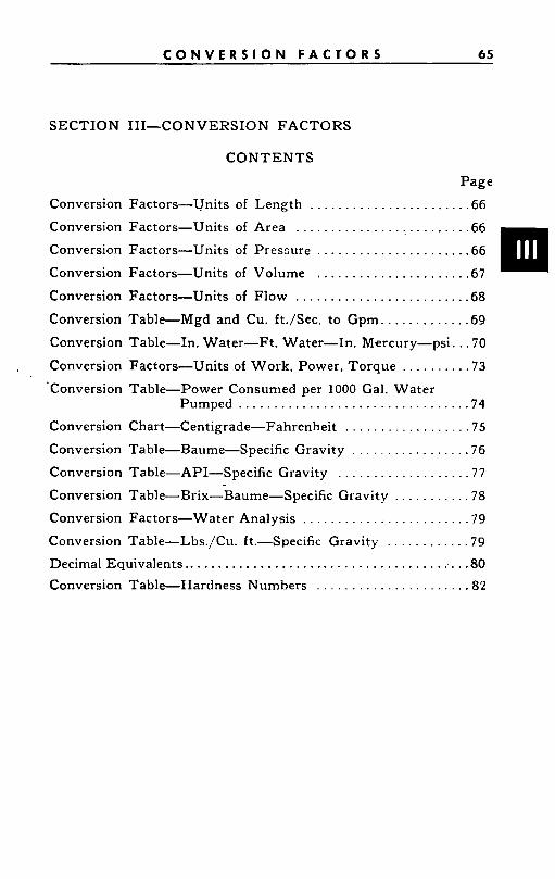
C O N V E R S I O N F A C T O R S 65
SECTION 111-CONVERSION FACTORS
CONTENTS
Page Conversion Factors-Units of Length ....................... 66 Conversion Factors-Units of Area .......................... 66
Conversion Factors-Units of Pressure ...................... 66 Conversion Factors-Units of Volume ...................... 67
Conversion Factors-Units of Flow ......................... 68
Conversion Table-Mgd and Cu . ft./Sec. to Gpm . . . . . . . . . . . . . 69
Conversion Table-In . Water-Ft . Water-In . Mercury-psi . . . 70
Conversion Factors-Units of Work. Power. Torque . . . . . . . . . . 73 . 'Conversion Table-Power Consumed per 1000 Gal . Water
Pumped . . . . . . . . . . . . . . . . . . . . . . . . . . . . . . . . . 74
Conversion Chart-Centigrade-Fahrenheit . . . . . . . . . . . . . . . . . . 75 Conversion Table-Baume-Specific Gravity . . . . . . . . . . . . . . . . . 76
Conversion Table-API-Specific Gravity . . . . . . . . . . . . . . . . . . . 77
Conversion Table-Brix-Baume-Specific Gravity . . . . . . . . . . . 7 8
Conversion Factors-Water Analysis . . . . . . . . . . . . . . . . . . . . . . . . 79
Conversion Table-Lbs./Cu. ft.-Specific Gravity . . . . . . . . . . . . 7 9
Decimal Equivalents .......................................... 80 Conversion Table-Hardness Numbers . . . . . . . . . . . . . . . . . . . . . . 8 2
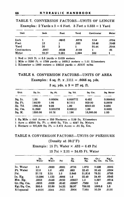
66 H Y D R A U L I C H A N D B O O K
TABLE 7. CONVERSION FACTORS-UNITS OF LENGTH Examples: 2 Yards x 3 = 6 Feet. 3 Feet x 0.333 = 1 Yard
Unit Inch Foot Yard Centimeter Meter
Inch 1 .0833 .0278 2.54 .0254 Foot 12 1 .333 30.48 .3048 Yard 36 3 1 91.44 .9144 Centimeters .3937 .0328 .0109 1 .01 Meter 39.37 3.281 1.094 100 1
1 Rod = 16.5 f t . = 5.5 yards = 5.029 meters 1 Mile = 5280 f t . = 1760 yards = 1609.3 meters = 1.61 Kilometers 1 Kilometer = 1000 meters = 1093.6 yards = .62137 miles
TABLE 8. CONVERSION FACTORS-UNITS OF AREA Examples: 6 sq. ft. x .1111 = .6666 sq. yds.
3 sq. yds. x 9 = 27 sq. ft.
Unit Sq. In. sq. Ft. Sq. Yd. Sq. Cm. Sq. Meter
Sq. In. 1.00 0.00694 0.000772 6.452 0.000645 Sq. Ft. 144.00 1.00 0.1111 929.00 0.0929 Sq. Yd. 1296.00 9.00 1.00 8360.00 0.836 Sq. Cm. 0.1550 0.001076 0.00012 1.00 0.0001 Sq. M. 1550.00 10.76 1.196 10,000.00 1.00
1 Sq Mile = 640 Acres = 259 Hectares = 2.59 Sq. Kilometers 1 Acre = 43560 Sq. Ft. = 4840 Sq. Yds. = 4047 Sq. Meters 1 Hectare = 107,639 Sq. Ft. = 2.471 Acres = .01 Sq. Km.
TABLE 9. CONVERSION FACTORS-UNITS OF PRESSURE
(Density at 39.2"F) Example: 15 Ft. Water X .433 = 6.49 Psi
15 Psi x 2.31 = 34.65 Ft. Water
In. Ft. In. Mm. GI./ Kg./ Water Water Psi Hg. Hg. Sq.Cm. Sp.Cm.
In. Water Ft. Water Psi. In. Hg. Mm. Hg. Gr./Sq. Cm. Kg./Sq. Cm. Kilopascal
1.0 12.0 27.72 13.696 .5353 .3936 393.6 4.0135
.0833 .0361 1.0 .433 2.31 1.0 1.133 .4906 .0446 .0193 .0328 .0142 32.80 14.22 .3344 .1451
.0736 3 8 3 2.040 1 .o .03937 .02897 28.97 .2954
1.870 22.43 51.816 26.40 1.0 .7360 736.03 7.505
2.538 30.45 70.31 34.49 1.357 1.0 1000.0 10.20
.0025
.0304
.0703
.0345
.0014
.001 1.0 .0102
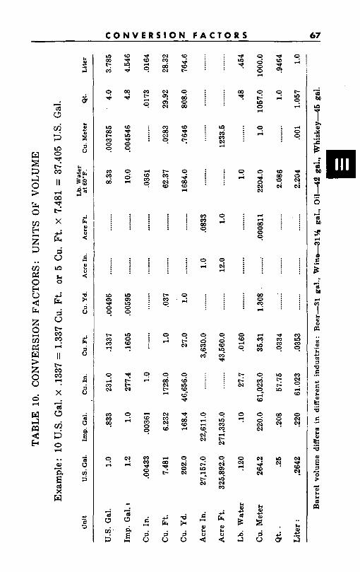
C O N V E R S I O N F A C T O R S 67
La 00 s 2
In 00 t- m 0 9
m 2
v) 0, d 0 9
t- m m :
2 m N
m
09 m
2
c
d 4 3
d W rl 9
m t- 4
9
d W m 9
2
d W 0 m
9
m m d 0 9
d 5 Y
u
N
2
2
N
N
N
m 00 N 9
I?
W x
t- m 9
2
2 N t- rl
N m 2
4 a f
J F 5 u
w W s
00 4
s
0 W d
9
P- t- N
0
0 N --!
5 B n !A
8
F
2
0 2
W 0 4
9 e 0 N N
rl rl
0 0 m
9
00 0
rl e?
d
16 F)
e?
9
0-
m N
d W
2 N N
4 W nr
! E 5 u
9 rl
t- W
d 9
4 0 9
d 0
eu N
m v) m 9
m N
4 W 9
0 N E!
N w W 4
3 3
- m M
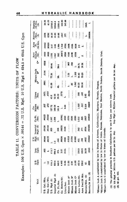
68 H Y D R A U L I C H A N D B O O K
. x
- - - “ N E c c c
P F P
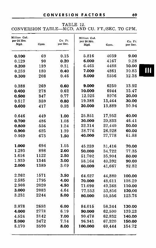
C O N V E R S I O N F A C T O R S 69
TAELE 12. CONVERSION TACLE-MGD. AND CU. FT./SEC. TO GPM.
Million Gal. per 24 Hrs. Cu. Ft.
Mgd. Gpm. per Sec.
0.100 0.129 0.200 0.259 0.300
0.388 0.400 0.500 0.617 0.600
0.646 0.700 0.800 0.900 0.969
1 .ooo 1.293 1.616 1.939 2.000
2.262 2.585 2.908 3.000 3.231
3.878 4.000 4.524 5.000 5.170
69 90
139 180 208
269 278 347 359 417
449 486 556 625 673
694 898
1122 1346 1389
1571 1795 2020 2083 2244
2693 2778 3142 3472 3590
0.15 0.20 0.31 0.40 0.46
0.60 0.62 0.77 0.80 0.93
1 .oo 1.08 1.24 1.39 1.50
1.55 2.00 2.50 3.00 3.09
3.50 4.00 4.50 4.64 5.00
6.00 6.19 7.00 7.74 8.00
Million Gal. per 24 Hrs. Cu. Ft.
Mgd. Gpm. per Sec.
5.816 6.000 6.463 7.000 8.000
9.000 10.000 12.925 19.388 20.000
25.851 30.000 32.314 38.776 40.000
45.239 50.000 51.702 58.164 60.000
64.627 70.000 71.090 77.553 80.000
84.015 90.000 90.478 96.941
100.000
4039 4167 4488 4861 5556
6250 6944 8976
13,464 13,889
17,952 20,833 22,440 26,928 27,778
31,416 34,722 35,904 40,392 41,667
44,880 48,611 49,368 53,856 55,556
58,344 62,500 62,832 67,320 69,444
9.00 9.28
13.92 15.47 20.00 30.00 30.94
40.00 46.41 50.00 60.00 61.88
70.00 77.35 80.00 90.00 92.82
100.00 108.29 1 10.00 120.00 123.76
130.00 139.23 140.00 150.00 154.72
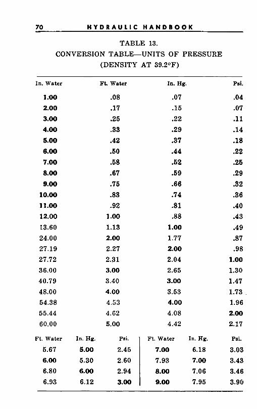
70 H Y D R A U L I C H A N D B O O K
In. Hg. Psi.
5.00 2.45 5.30 2.60 6.00 2.94 6.12 3.00
TABLE 13. CONVERSION TABLE-UNITS OF PRESSURE
(DENSITY AT 39.2OF)
Ft. Water In. Hg.
7.00 6.18 7.93 7.00 8.00 7.06 9.00 7.95
In. Water
1 .QO
2.00 3.00 4.00 5.00 6.00 7.00 8.00
9.00 10.00 11.00 12.00
13.60 24.00 27.19 27.72 36.00 40.79 48.00 54.38 55.44 60.00
Ft. Water
6.67 6.00
6.80 6.93
Psi.
.04
.07
.ll
.14
.18
.22
.26
.29 3 2 .36 .40 .43 .49 .87 .98
1 .oo 1.30 1.47 1.73 ,
1.96 2.00
2.17
Psi.
3.03 3.43 3.46 3.90
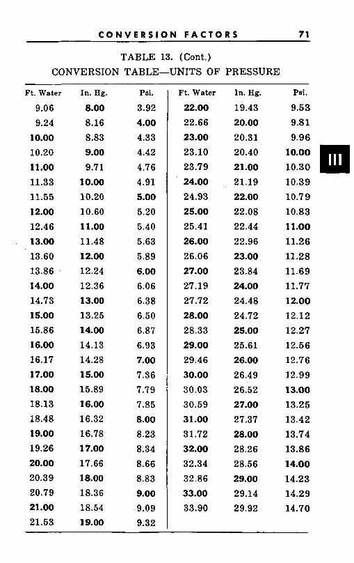
C O N V E R S I O N F A C T O R S 71 ~~ ~ ~~
TABLE 13. (Cont.)
CONVERSION TABLE-UNITS OF PRESSURE
Ft. Water
9.06 9.24
10.00
10.20 11 .oo 11.33 11.55 12.00
12.46 13.00
13.60 13.86 .
14.00
14.73 15.00
15.86 16.00
16.17 17.00
18.00
18.13 18.48 19.00
19.26 20.00
20.39 20.79 21.00
21.53
In. Hg.
8.00 8.16 8.83 9.00
9.71 10.00
10.20 10.60 11 .oo 11.48 12.00
12.24 12.36 13.00
13.25 14.00
14.13 14.28 15.00
15.89 16.00
16.32 16.78 17.00
17.66 18.00
18.36 18.54 19.00
Psi.
3.92 4.00
4.33 4.42 4.76 4.91 5.00
5.20 5.40 5.63 5.89 6.00 6.06 6.38 6.50 6.87 6.93 7.00
7.36 7.79 7.85 8.00
8.23 8.34 8.66 8.83 9.00
9-09 9.32
Ft. Water
22.00
22.66 23.00
23.10 23.79 24.00
24.93 25.00
25.41 26.00
26.06 27.00
27.19 27.72 28.00
28.33 29.00
29.46 30.00 30.03 30.59 31.00
31.72 32.00
32.34 32.86 33.00
33.90
In. Hg.
19.43 20.00 20.31 20.40 21.00
21.19 22.00
22.08 22.44 22.96 23.00
23.84 24.00
24.48 24.72 25.00
25.61 26.00
26.49 26.52 27.00
27.37 28.00
28.26 28.56 29.00
29.14 29.92
Psi.
9.53 9.81 9.96
10.00
10.30 10.39 10.79 10.83 11.00
11.26 11.28 11.69 11.77 12.00
12.12 12.27 12.56 12.76 12.99 13.00
13.25 13.42 13.74 13.86 14.00
14.23 14.29 14.70
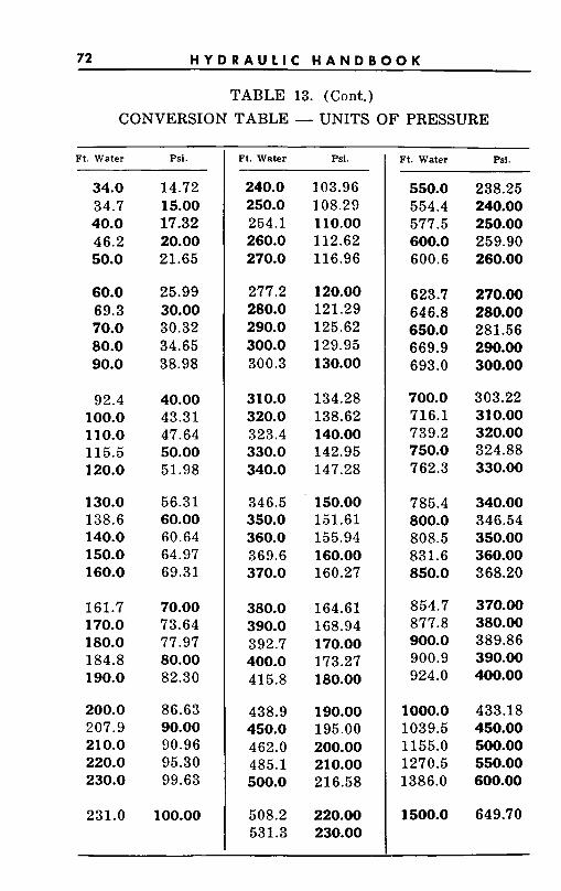
72 H Y D R A U L I C H A N D B O O K
TABLE 13. (Cont.) CONVERSION TABLE - UNITS O F PRESSURE
Ft. Water Psi.
34.0 34.7 40.0 46.2 50.0
60.0 69.3 70.0 80.0 90.0
92.4 100.0 1 10.0 115.5 120.0
130.0 138.6 140.0 150.0 160.0
161.7 170.0 180.0 184.8 190.0
200.0 207.9 21 0.0 220.0 230.0
231.0
14.72 15.00 17.32 20.00 21.65
25.99 30.00 30.32 34.65 38.98
40.00 43.31 47.64 50.00 51.98
56.31 60.00 60.64 64.97 69.31
70.00 73.64 77.97 80.00 82.30
86.63 90.00 90.96 95.30 99.63
100.00
Ft. Water Psi.
240.0 250.0 254.1 260.0 270.0
277.2 280.0 290.0 300.0 300.3
310.0 320.0 323.4 330.0 340.0
346.5 350.0 360.0 369.6 370.0
380.0 390.0 392.7 400.0 415.8
438.9 450.0 462.0 485.1 500.0
508.2 531.3
103.96 108.29 1 10.00 112.62 116.96
120.00 121.29 125.62 129.95 130.00
134.28 138.62 140.00 142.95 147.28
150.00 151.61 155.94 160.00 160.27
164.61 168.94 170.00 173.27 180.00
190.00 195.00 200.00 210.00 216.58
220.00 230.00
Ft. Water Psi.
550.0 554.4 577.5 600.0 600.6
623.7 646.8 650.0 669.9 693.0
700.0 716.1 739.2 750.0 762.3
785.4 800.0 808.5 831.6 850.0
854.7 877.8 900.0 900.9 924.0
1000.0 1039.5 1155.0 1270.5 1386.0
1500.0
238.25 240.00 250.00 259.90 260.00
270.00 280.00 281.56 290.00 300.00
303.22 310.00 320.00 324.88 330.00
340.00 346.54 350.00 360.00 368.20
370.00 380.00 389.86 390.00 400.00
433.18 450.00 500.00 550.00 600.00
649.70
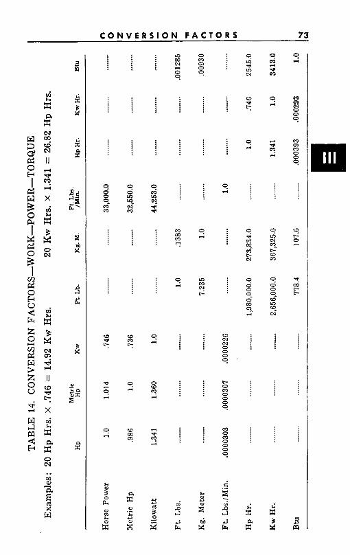
C O N V E R S I O N F A C T O R S 73
2 3 ua
m
(0 m c:
9 rl
W m Q!
x”
; U
SA U .-
In N rl 0
m
9
i
M m m I
9 rl
i i
ui f; j a
0
c1 0
m
9
9 rl
In m
2
& U
; 2
9 3
W N N 0 0 0 9
P- 0 m 0 0 0 9
m 0 m 0 0 0 9
d 2 -2 .n 4 d a
5
m 0, N 0 0 9
m 0, m 0 0 9
: 0 4
4 00 P- c1
7 G
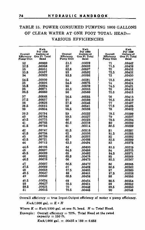
74 H Y D R A U L I C H A N D B O O K ~
TABLE 15. POWER CONSUMED PUMPING 1000 GALLONS OF CLEAR WATER AT ONE FOOT TOTAL HEAD-
VARIOUS EFFICIENCIES
Kwh Per 1000
Overall Gallons at Efficiency One Ft. Total PumpUnit Head
32 32.6 33 33.6 34 34.6 36 35.5 36 36.6 37 37.6 38 38.6 39 39.6 40 40.5 41 41.6 42 42.6 43 43.6 44 44.6 45 45.6 46 46.6 47 47.6 48 48.5 49 49.6 50 50.5 51
.00980
.00958
.00951
.00937
.00922
.00909
.00896
.00884
.00871
.00860
.00848
.00837
.00826
.00816
.00804
.00794
.00784
.00775
.00765
.00756
.00747 A0738 .00730 .00721 .00713 .00706 .00697 .00689 .00682 .00675 .00667 .00660 .00653 .00647 .00640 .00634 .00627 .00621 .00616
Overall Efficiency Pump Unit
51.6 52 52.6 53 53.6 54 54.5 66 55.5 56 56.6 67 57.6 58 58.5 59 59.6 60 60.5 61 61.6 62 62.5 63 63.5 64 64.5 65 65.5 66 66;6 67 67.5 68 68.6 69 69.6 70 70.6
Kwh Per 1000
Gallons at One Ft. Total
Head
.00609
.00603
.00597
.00592
.00586
.00581
.00576
.00570
.00565
.00560
.00555
.00550
.00546
.00541
.00536
.00532
.00527
.00523
.00518
.00514
.00510
.00506
.00602
.00498
.00494
.00490
.00486
.00482
.00479
.00475
.00472
.00468
.00465
.00461
.00458
.00454 -00451 .00448 .00446
Overall Efficiency Pump Unit
71 71.6 72 72.6 73 73.6 74 74.5 75 75.5 76 76.5 77 77.6 78 78.6 79 79.6 80 80.6 81 81.6 82 82.5 83 83.5 84 84.6 85 85.6 86 86.5 87 87.5 88 88.6 89 89.6 90
Kwh Per loo0
Gallons at One Ft. Tohl
Head
.00442
.00439
.00435 b0432 .00430 .00427 .00424 .00421 .00418 .00415 .00413 .00410 .00407 .00405 .00402 .00399 .00397 .00394 .00392 .00389 .00387 .00385 .00382 .00380 .00378 .00376 .00373 .00371 .00369 .00367 .00366 -00362 -00360 .00358 .00356 .00354 .00352 .00360 .00348
Overall efficiency = true Input-Output efficiency of motor x pump efficiency.
KwhI1000 gal, = K H Where K = Kwhf1000 gal. a t one ft. head. H = Total Head. Example: Overall efficiency = 72%. Total Head a t the rated
capacity = 150 f t . Kwh11000 gal. = .00436 x 160 = 0.653
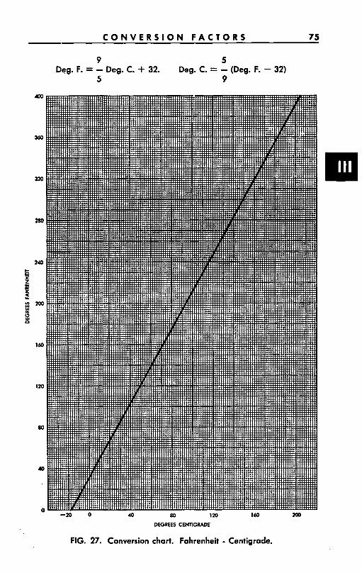
C O N V E R S I O N F A C T O R S 75 - 9 5
Deg. F. = - Dee. C. + 32. Deg. C. = - (Deg. F. - 32) 5 9
C
"ES CENnCRADE
FIG. 27. Conversion chart. Fahrenheit - Centigrade.
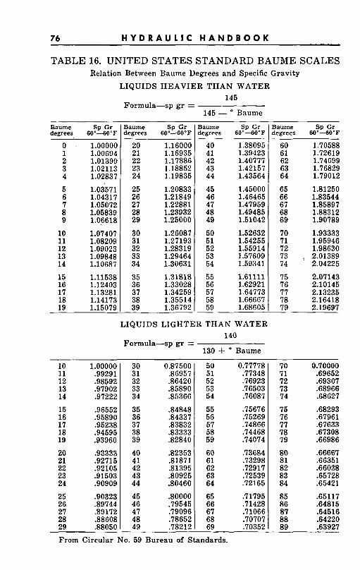
76 H Y D R A U L I C H A N D B O O K
Baume Sp Gr degrees 60"-60'F
20 1.16000 21 1.16935 22 1.17886 23 1.18852 24 1.19835 25 1.20833 26 1.21849
TABLE 16. UNITED STATES STANDARD BAUME SCALES Relation Between Baume Degrees and Specific Gravity
LIQUIDS HEAVIER THAN WATER
Baume Sp G r degrees 60'40°F
40 1.38095 41 1.39423 42 1.40777 43 1.42157 44 1.43564 45 1.45000 46 1.46465
Baume Sp Gr degrees 60"-60"F
27 i.22881 28 1.23932 29 1.25000 30 1.26087 31 1.27193 32 1.28319
0 ' 1.00000 1 1.00694
47 1.47959 48 1.49485 49 1.51042 50 1.52632 51 1.54255 52 1.55914
2 1.01399 3 1.02113 4 1.02837
33 1.29464 34 1.30631 35 1.31818 36 1.33028 37 1.34259
5 1.03571
53 1.57609 54 1.59341 55 1.61 111 56 1.62921 57 1.64773
6 1.04317 7 1.05072 8 1.05839
31 .86957 32 .86420 33 A5890 34 35366
9 1.06618
10 1.07407 11 1.08209 12 1.09023 13 1.09848 14 1.10687 15 1.11538 16 1.12403
51 52 53 54
17 1.13281 18 1.14173 19 1.15079
.- ~~ ~- ~~
36 .84337 37 33832 38 33333
10 1.00000
56 57 58
11 .99291 12 .98592 13 .97902
40 .82353 41 31871 42 .81395
14 .97222
60 61 62
15 .96552 16 .95890 17 .95238
43 .80925 44 30460 45 .80000 46 .79545 47 .79096 48 .78652 49 .78212
18 .94595 19 .93960
63 64
65 66 67 68 69
20 .93333 21 .92715 22 .92105 23 .91503 24 .go909 25 .go323 26 39744 27 .89172 28 38608 29 .88050
1.66667 1.68605
38 39
LIQUIDS LIGHTER THAN WATER 140
130 4- Baume Formula-sp gr =
30 0.875001 50
35 -848481 55
39 328401 59
~
3aume Sp Gr iegrees 60'40°F
0.77778 .77348 .76923 .76503 .76087 .75676 .75269 .74866 .74468 .74074 .73684 .73298 .72917 .72539 .72165
.71795
.71428
.71066
.70707
.70352
60 1.70588 61 1.72619 62 1.74699 63 1.76829 64 1.79012 65 1.8 1250 66 1.83544 ~ _~ .__
67 1.85897 68 1.88312 69 1.90789 70 1.93333 71 1.95946 72 1.98630 73 2.01389 74 2.04225 75 2.07143 76 2.10145 77 2.13235 78 2.16418 79 2.19697
$0 0.7 0 0 0 0 71 .69652 72 .69307 73 .68966 74 .68627 75 .68293 76 .67961 77 .67633 78 .67308 79 .66986 so .66667 -.
81 .66351 82 .66038 83 .65728 84 .65421 85 -65117 86 .64815 87 .64516 88 .64220 89 .63927
From Circular No. 59 Bureau of Standards.
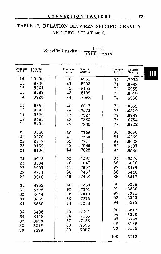
C O N V E R S I O N F A C T O R S 77
TABLE 17. RELATION BETWEEN SPECIFIC GRAVITY AND DEG. API AT 60°F.
141.5 131.5 + "API
Specific Gravity = --
Degrees Specific A.P.I. Gravity
10 1.0000 11 .9930 12 .9861 13 .9792 14 .9725
15 .9659 16 .9593 17 .9529 18 .9465 19 .9402
20 .9340 21 .9279 22 .9218 23 .9159 24 .9100
25 .9042 26 .8984 27 .8927 28 .8871 29 .8816
30 .8762 31 .8708 32 .8654 33 .8602 34 .8550
35 .8498 36 .8448 37 .8398 38 .8348 39 .8299
Degrees A.P.I.
40 41 42 43 44
45 46 47 48 49
50 51 52 53 54
55 56 57 58 59
60 61 62 63 64
65 66 67 68 69
Specific Gravity
.8251
.8203
.8155
.8109 .8063
.8017
.7972
.7927
.7883
.7839
.7796
.7753
.7711
.7669
.7628
.7587
.7547
.7507
.7467
.7428
.7389
.7351
.7313
.7275
.7238
.7201
.7165
.7128
.7093
.7057
Degrees A.F.1.
70 71 72 73 74
75 76 77 78 79
80 81 82 83 84
85 86 87 88 89
90 91 92 93 94
95 96 97 98 99
100
.6988
.6952
.6919
.6886
.6852
.6819
.6787
.6754
.6722
.6690
.6659
.6628
.6597
.6566
.6536
.6506
.6476
.6446
.6417
.6388
.6360
.6331
.6303
.6275
.6247
.6220
.6193
.6166
.6139
.6112
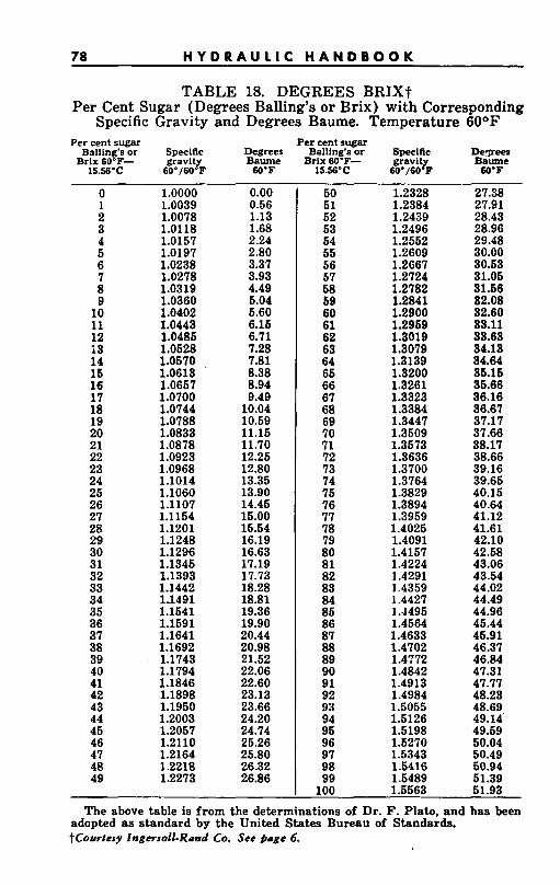
78 H Y D R A U L I C H A N D B O O K
TABLE 18. DEGREES BRIX? Per Cent Sugar (Degrees Balling's or Brix) with Corresponding
Specific Gravity and Degrees Baume. Temperature 60°F Per cent sugar Per cent sugar
Balling's or Speclfic Degrees Balllng's or Specific De.- Baume
60.F Brix 60-F- gravity Baume Brix 60-F- l?y'?.
15.56'C 60'/60'F 60'F 15.56'C 60 /60 F
0 1 2 3 4 5 6 7 8 9 10 11 12 i3 14 15 16 17 18 19 20 21 22 23 24 25 26 27 28 29 30 31 32 33 34 35 36 37 38 39 40 41 42 43 44 45 46 47 48 49
1.0000 1.0039 1.0078 1.0118 1.0157 1.0197 1.0238 1.0278
1.0360 1.8402 1.0443 1.0485 1.0628 1.0670 1.0613 1.0657 1.0700 1.0744 1.0788 1.0833 1.0878 1.0923 1.0968 1.1014 1.1060 1.1107 1.1154 1.1201 1.1248 1.1296 1.1345 1.1393 1.1442 11491 1.1541 1.1591 1.1641 1.1692 1.1743 1.1794 1.1846 1.1898 1.1950 1.2003 1.2057 1.2110 1.2164 1.2218 1.2273
1.0319
0.00 0.56 1.13 1.68 2.24 2.80 3.37 3.93 4.49 5.04 5.60 6.16 6.71 7.28 7.81 8.38 8.94 9.40 10.04 10.69 11.15 11.70 12.25 12.80 13.35 13.90 14.45 15.00 15.54 16.19 16.63 17.19 17.73 18.28 18.81 19.36 19-90 20.44 20.98 21.52 22.06 22.60 23.13 23.66 24.20 24.74 26.26 25.80 26.32 26.86
50 51 52 53 54 55 56 57 58 59 60 61 62 63 64 65 66 67 68 69 70 71 72 73 74 75 76 77 78 79 80 81 82 83 84 85 86 87 88 89 90 91 92 93 94 95 96 97 98
1.2328 1.2384 1.2439 1.2496 1.2552 1.2609 1.2667 1.2724 1.2782 1.2841 1.2900 1.2959 1.3019 1.3079 1.3139 1.3200 1.3261 1.3323 1.3384 1.3447 1.3509 1.3573 1.3636 1.3700 1.3764 1.3829 1.3894 1.3959 1.4025 1.4091 1.4157 1.4224 1.4291 I .4359 I .4427 1 A495 1.4564 1.4633 1.4702 1.4772 1.4842 1.4913 1.4984 1.5055 1.5126 1.5198 1.6270 1.5343 1.5416
27.38 27.91 28.43 28.96 29.48 30.00 30.53 31.05 31.56 32.08 32.60 33.11 33.63 34.13 34.64 35.15 35.66 36.16 36.67 37.17 37.66 38.17 38.66 39.16 39.65 40.15 40.64 41.12 41.61 42.10 42.58 43.06 43.54 44.02 44.49 44.96 45.44 45.91 46.37 46.84 47.31 47.77 48.23 48.69 49.14. 49.59 50.04 50.49 50.94
99 1.5489 51.39 100 1.5563 51.93
The above table is from the determinations of Dr. F. Plato, and has been adopted as standard by the United States Bureau of Standards. tCourtesy Ingusoll-Rand Co. See Page 6.
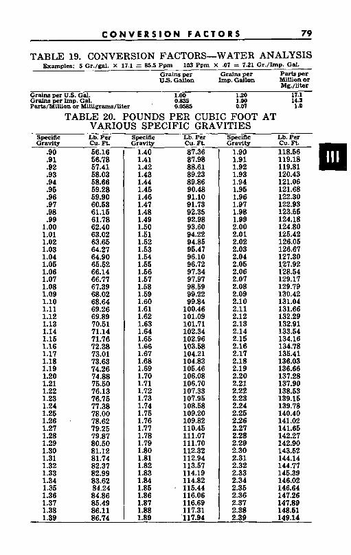
C O N V E R S I O N F A C T O R S 79
specific Lb. Per Specific Lb. Per Gravity Cu.Ft. Gravity cu. Ft.
.90 66.16 1.40 87.36
TABLE 19. CONVERSION FACTORS-WATER ANALYSIS
Grains per Grains per Parts per US. Gallon Imp. Gallon Million or
Mg./liter
Examples: 5 Gr./gal. X 17.1 = 85.5 Ppm 103 Ppm X .07 7.21 Gr./lmp. Gal.
Specific Lb. P e r Gravity cu. Ft. 1.90 118.66
119.18 119.81 120.43 121.06
Grains per US. Gal. Grains per Imp. Gal. Parts/MilUon or MilUgrams/liter '
1.88 ~~ ~~
1.89 117.94
~~
1 .00 0.835 0.0585
148.61 2.39 149.14
1.20 1.00 0.07
TABLE 20. POUNDS PER CUBIC FOOT AT VARIOUS SPECIFIC GRAVITIES
17.1 14.3 1 .o
.91
.92
.93
.94
.96
.96
.97
.98
.99 1.00 1.01 1.02 1.03 1.04 1.06 1.06 1.07 1.08 1.09 1.10 1.11 1.12 1.13 1.14 1.16 1.16 1.17 1.18 1.19 1.20 1.21 1.22 1.23 1.24 1.26 1.26 1.27 1.28 1.29 1.30 1.31 1.32 1.33 1.34 1.36 1.36 1.37
66.78 67.41 68.03 68.66 69.28 69.90 60.63 61.16 61.78 62.40 63.02 63.66 64.27 64.90 66.62 66.14 66.77 67.39 68.02 68.64 69.26 69.89 70.61 71.14 71.76 72.38 73.01 73.63 74.26 74.88 76.50 76.13 76.76 77.38 78.00 78.62 79.25 79.87 80.50 81.12 81.74 82.37 82.99 83.62 84.24 84.86 86.49
1.38 86.11 1.39 86.74
1.41 1.42 1.43 1.44 1.46 1.46 1.47 1.48 1.49 1.60 1.61 1.62 1.63 1.64 1.66 1.66 1.67 1.58 1.69 1.60 1.61 1.62 1.63 1.64 1.66 1.66 1.67 1.68 1.69 1.70 1.71 1.72 1.73 1.74 1.75 1.76 1.77 1.78 1.79 1.80 1.81 1.82 1.83 1.84 1.86 1.86 1.87
87.98 88.61 89.23 89.86 90.48 91.10 91.73 92.36 92.98 93.60 94.22 94.86 96.47 96.10 96.72 97.34 97.97 98.69 99.22 99.84 100.46 101.09 101.71 102.34 102.96 103.68 104.21 104.83 106.46 106.08 106.70 107.33 107.95 108.68 109.20 109.82 110.45 111.07 111.70 112.32 112.94 113.67 114.19 114.82 116.44 116.06 116.69 117.31
1.91 1.92 1.93 1.94 1.96 1.96 1.97 1.98 1.99 2.00 2.01 2.02 2.03 2.04 2.06 2.06 2.07 2.08 2.09 2.10 2.11 2.12 2.13 2.14 2.16 2.16 2.17 2.18 2.19 2.20 2.21 2.22 2.23 2.24 2.26 2.26 2.27 2.28 2.29 2.30 2.31 2.32 2.33 2.34 2.35 2.36 2.37 2.38
121.68 122.30 122.93 123.66 124.18 124.80 126.42 126.06 126.67 127.30 127.92 128.64 129.17 129.79 130.42 131.04 131.66 132.29 132.91 133.54 134.16 134.78 136.41 136.03 136.66 137.28 137.90 138.63 139.16 139.78 140.40 141.02 141.66 142.27 142.90 143.62 144.14 144.77 146.39 146.02 146.64 147.26 147.89
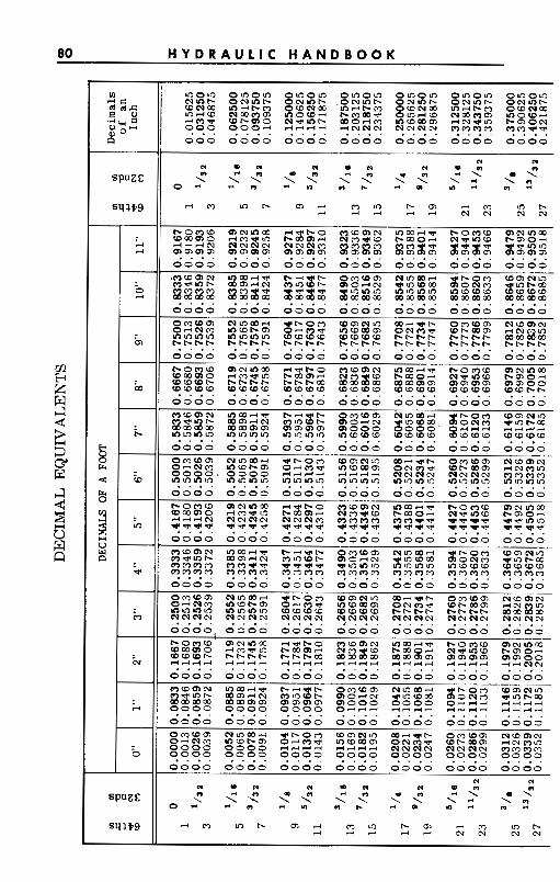
80 H Y D R A U L I C H A N D B O O K
m
m -
h
w
u,
*
N
In010 olnoln olnoln olnoln olnoln olnoln olnoln N m b O N m b O N m b . O N u a b O N m b O N m b O"+ W" m 4 t - m O " W n 3 t - m O W " m 4 t - m O W " m r l w ~ m m m m o w 4 b m m e o l n r l w ~ m m m m o w d 4 m - F w + m o N * m + m o r l m m w m m r lN* ln b m O N
0 0 0 0000 0000 0000 0000 0000 0000 999 9991 q1q1 ?@??PI N.N.N.? ???? 1144
. . . . . . . . . . . . . . . . . . . . . . . . . . . . . . . . . . . . 0000 0000 0000 0000 0000 0000 0000 ~~~
t - o m w m m m m rl-t-0 m w m ~ moor(+ t - o m w m ~ m m w m m o d m w l n t - m m d t - w o d N W ~ W t - m o r l w w w b t-bt-b t - b t - m 2 Z S Z m m m m m m m m m m o o w w w w w w w w 9 F W - W w w w w w m w w w w w w w w t - b . . . . . . . . . . . . . . . . . . . . . . .
0000 0000
2:s: 882% m m m m m o o o u a m m l n m w w w
. . 0000 0000 0000
. . . . . . . . . . . . . . . . . . . . . . . . . . . . 0000 0000 0000 0000 0000 0000 0000
. . . . . . . . . . . . . . . . . . . . . . . . . . . . 0000 0000 0000 0000 0000 0000 0000 t - o m w m ~ m m rl-t-0 m w m ~ m m ~ v t - o m w m ~ m m w m m o r l m w m b m m d " a w + m o d Cu+mw b m o d r l 3 r l N "" NN" m m m m m m w + a*** * e l o m
0000 0000 0000 0000 0000 0000 0000 4 4 4 4 4444 4444 4444 4 4 4 4 3454 4444
0000 0000 0000 0000 0000 0000 0000
"" NN" "" "" "" NN" NN" . . . . . . . . . . . . . . . . . . . . . . . . 0000,0000 0000 0000 0000 0000 d o 0 0
dddd dddd ddd3 rlddd d d d d dddd d3"
0000 0000 0000 0000 0000 0300 0000 . . . . . . . . . . . . . . . . . . . . . . . . . . . .
0000 0000 0000 O d d 3 r l 3 I - l ' dddd ddd3
0000 0000 0000 0000 0000 0000 0000 o m w m "ad a b o m w m m l n m3*+ o m w m N w m N 04" uawt-m o d m v uawmm o m m w w b m m rleamm 0000 0000 ddd3 rldrld "" "" m m m n
0000 0000 0000 0000 0000 0000 0000
. . . . . . . . . . . . . . . . . . . . . . . . . . . .
9999 9999 9999 9999 9999 9999 9993 N N
N P O N O N N Q N
O M 3 0 0 -
3 m L o b m 3 m l n b m 3 m a r c 3 d 3 4 3 " N N
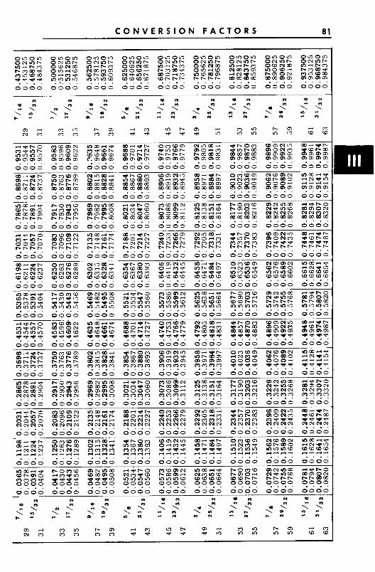
C O N V E R S I O N F A C T O R S 81
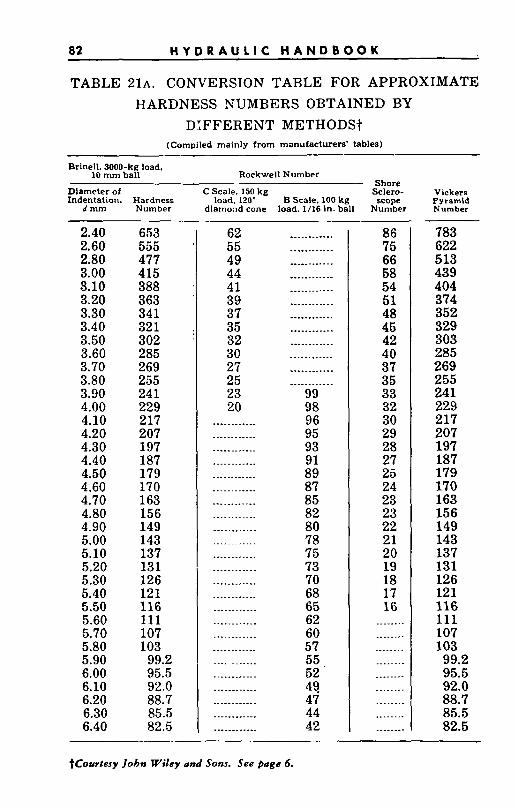
82 H Y D R A U L I C H A N D B O O K
TABLE 2 1 ~ . CONVERSION TABLE FOR APPROXIMATE HARDNESS NUMBERS OBTAINED BY
DIFFERENT METHODS? (Compiled mainly from manufacturers’ tables)
Brinell. 3000-kg load,
Dlameter of C Scale, 150 kg Sclero- Vickers Indentation. Hardness load, 120’ B Scale. 100 kg scope Pyramid
d m m Number diamond cone load, 1/16 in. ball Number Number
10 mm ball Rockwell Number Shore
2.40 2.60 2.80 3.00 3.10 3.20 3.30 3.40 3.50 3.60 3.70 3.80 3.90 4.00 4.10 4.20 4.30 4.40 4.50 4.60 4.70 4.80 4.90 5.00 5.10 5.20 5.30 5.40 5.50 5.60 5.70 5.80 5.90 6.00 6.10 6.20 6.30 6.40
653 555 477 415 388 363 34 1 321 302 285 269 255 241 229 2 17 207 197 187 179 170 163 156 149 143 137 131 126 121 116 111 107 103
99.2 95.5 92.0 88.7 85.5 82.5
62 55 49 44 4 1 39 37 35 32 30 27 25 23 20
............
............
............
............
............
............
............
............
............
............
...........
............
............
............
............
............
............
............
............
............
............
............
............
............
............
............
............ 99 98 96 95 93 91 89 87 85 82 80 78 75 73 70 68 65 62 60 57 55 52 4? 47 44 42
86 75 66 58 54 51 48 45 42 40 37 35 33 32 30 29 28 27 25 24 23 23 22 21 20 19 18 17 16
_.._. _.. ........
........
........
........
........
.___ __..
783 622 513 439 404 374 352 329 303 285 269 255 241 229 217 207 197 187 179 170 163 156 149 143 137 131 126 121 116 111 107 103 99.2 95.5 92.0 88.7 85.5 82.5
tCorrtesy John Wiley and Sons. See Page 6.
W A T E R D A T A 83
SECTION IV-WATER DATA
CONTENTS Page
Properties of Water-Viscosity ............................. 84
Properties of Water-Vapor Pressure. Specific Weight . Table-Relation Altitude. Barometric Pressure. Atmospheric
Specific Gravity . . . . . . . . . . . . . . . . . . . . . . . 85
Pressure. Boiling Point of Water ..................... 86
Water Requirements-Feeding Boilers ...................... 87
Water Requirements-Industrial Plants ..................... 88
Water Requirements-Public Buildings ..................... 90
Water Requirements-Swimming Pools ..................... 91 Water Requirements-Hot Water Service . . . . . . . . . . . . . . . . . . . 92
Water Requirements-Rural and Domestic . . . . . . . . . . . . . . . . . . . 94
Water Requirements-Irrigation . . . . . . . . . . . . . . . . . . ; . . . . . . . . . 94 Land Drainage-Pumped Outlets ........................... 100
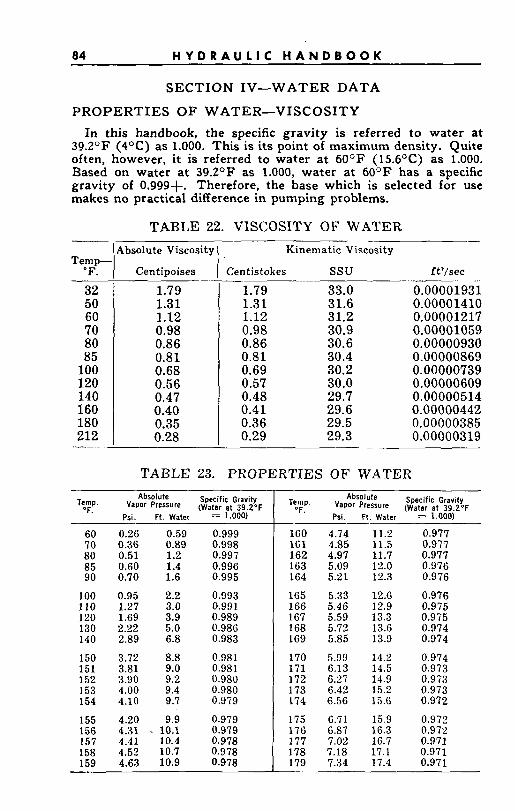
84 H Y D R A U L I C H A N D B O O K
Absolute Specific Gravity Temp. Vapor Pressure (water at 39.2”~ OF.
Psi. Ft. Water 1.000)
SECTION IV-WATER DATA
P R O P E R T I E S OF WATER-VISCOSITY In this handbook, the specific gravity is referred to water at
39.Z°F (4OC) as 1.000. This is its point of maximum density. Quite often, however, it is referred to water at 60°F (15.6OC) as 1.000. Based on water at 39.Z°F as 1.000, water at 60°F has a specific gravity of 0.999+. Therefore, the base which is selected for use makes no practical difference in pumping problems.
TABLE 22. VISCOSITY OF WATER
Specific Gravity TtmP, F. Vapor Pressure (Water at 39.2’F Psi. Ft. Water = 1.000)
Teemp- F.
60 0.26 0.59 0.999 70 0.36 0.89 0.998 80 0.51 1.2 0.997
32 50 60 70 80 85
100 120 140 160 180 212 -- ~
160 4.74 11.2 0.977 161 4.85 11.5 0.977 162 4.97 11.7 0.977
lbsolute Viscosity
Cen tiDoises
--. -~ 120 1.69 3.9 0.989 130 2.22 5.0 0.986 140 2.89 6.8 0.983
1.79 1.31 1.12 0.98 0.86 0.81 0.68 0.56 0.47 0.40 0.35 0.28
167 5.59 13.3 0.975 168 5.72 13.6 0.974 169 5.85 13.9 0.974
Kinematic Viscosity
Centistokes ssu f t’/sec
_-.
151 3.81 9.0 0.981 152 3.90 9.2 0.980 153 4.00 9.4 0.980
1.79 1.31 1.12 0.98 0.86 0.81 0.69 0.57 0.48 0.41 0.36 0.29
171 6.13 14.5 0.973 172 6.27 14.9 0.973 173 6.42 15.2 0.973
33.0 31.6 31.2 30.9 30.6 30.4 30.2 30.0 29.7 29.6 29.5 29.3
154 4.10 9.7 0.979
155 4.20 9.9 0.979 156 4.31 . 10.1 0.979 157 4.41 10.4 0.978 158 4.52 10.7 0.978 159 4.63 10.9 0.978
0.00001931 0.00001410 0.00001217 0.00001059 0.00000930 0.00000869 0.00000739 0.00000609 0.00000514 0.00000442 0.00000385 0.00000319
174 6.56 15.6 0.972
175 6.71 15.9 0.972 176 6.87 16.3 0.972 177 7.02 16.7 0.971 178 7.18 17.1 0.971 179 7.34 17.4 0.971
TABLE 23. PROPERTIES O F WATER
-.
85 0.60 1.4 0.996 163 5.09 18.0 0.976 90 0.70 1.6 0.995 I 164 5.21 12.3 0.976
100 0.95 2.2 0.993 165 5.33 12.6 0.976 110 1.27 3.0 0.991 I 166 5.46 12.9 0.975
150 3.72 8.8 0.981 1 170 5.99 14.2 0.974
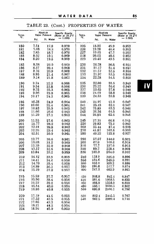
W A T E R D A T A 85
TABLE 23. (Cont.) PROPERTIES O F WATER
180 181 182 183 184
185 186 187 188 189
190 191 192 193 194
195 196 197 198 199
200 201 202 203 204
205 206 207 208 209 210 21 1 212 213 214
215 216 217 218 219
220 22 1 222 223 224
7.51 7.68 7.85 8.02 8.20
8.38 8.57 8.76 8.95 9.14
9.34 9.54 9.75 9.96
10.17
10.38 10.60 10.83 11.06 11.29
11.53 11 .77 12.01 12.26 12.51
12.77 13.03 13.30 13.57 13.84 14.12 14.41 14.70 14.99 15.29
15.59 15.90 16.22 16.54 1G.86
17.19 17.52 17.86 18.21 18.56
17.8 18.3 18.7 19.1 19.5
20.0 20.4 20.9 21.4 21.8
22.3 22.8 23.3 23.8 24.3
24.9 25.4 25.9 26.6 27.1
27.6 28.2 28.8 29.4 30.0
30.6 31.2 32.0 32.6 33.2 33.9 34.6 35.4 36.2 37.0
37.7 38.4 39.2 40.0 40.8
41.6 42.5 43.3 44.2 45.0
0.970 0.970 0.970 0.969 0.969
0.969 0.968 0.968 0.967 0.967
0.966 0.966 0.965 0.965 0.965
0.964 0.964 0.963 0.963 0.963
0.963 0.962 0.962 0.962 0.961
0.961 0.960 0.960 0.960 0.959 0.959 0.958 0.958 0.957 0.957
0.957 0.956 0.956 0.956 0.955
0.955 0.955 0.954 0.954 0.953
Absol Ute Specific Gravity Temp. Vapor Pressure (Water at 39.2"F
Psi. Ft. Water l'ooo) OF.
225 226 227 228 229
230 231 232 233 234
235 236 237 238 239
240 241 242 243 244
245 250 260 270 280
290 300 310 320 330 340 350 360 380 400
420 440 460 480 500
s20 540
18.92 19.28 19.65 20.02 20.40
20.78 21.17 21.57 21.97 22.88
22.80 23.22 23.65 24.09 24.53
24.97 25.43 25.89 26.36 26.83
27.31 29.83 35.44 41.87 49.22
57.57 67.0 77.7 89.7
103.0 118.0 134.6 153.0 195.8 247.3
308.8 381.6 466.9 566.1 680.8
812.4 962.5
45.9 46.8 47.7 48.6 49.5
50.5 51.4 52.5 53.5 54.5
55.5 56.6 57.8 58.8 59.8
ti1.0 62.1 63.3 64.5 65.G
66.8 73.2 87.4
103.6 122.8
144.0 168.6 197.0 228.4 264.0 305.0 349.0 399.2 517.7 663.9
842.4 1058.5 1318.0 1630.5 2000.1
2445.5 2980.4
0.953 0.953 0.952 0.952 0.951
0.951 0.951 0.950 0.950 0.950
0.949 0.949 0.948 0.948 0.948
0.947 0.947 0.946 0.946 0.946
0.945 0.943 0.938 0.933 0.927
0.923 0.918 0.913 0.908 0.902 0.896 0.891 0.886 0.874 0.861
0.847 0.833 0.818 0.802 0.786
0.767 0.746
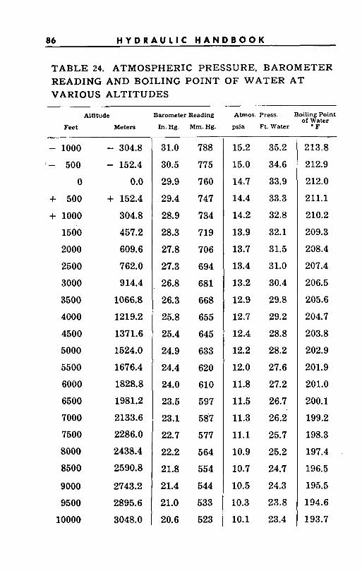
86 H Y D R A U L I C I I A N D B O O K
T A B L E 24. ATMOSPHERIC PRESSURE, BAROMETER READING AND BOILING P O I N T O F W A T E R A T VARIOUS A L T I T U D E S
Alfltude Barometer Reading
Feet Meters In. Hg. Mm. Hg.
Atmos. Press.
psia Ft. Water
- 1000
' - 500
0
+ 500
+ 1000
1500
2000
2500
3000
3500
4000
4500
5000
5500
6000
6500
7000
7500
8000
8500
9000
9500
10000
- 304.8
- 152.4
0.0
+ 152.4
304.8
457.2
609.6
762.0
914.4
1066.8
1219.2
1371.6
1524.0
1676.4
1828.8
1981.2
2133.6
2286.0
2438.4
2590.8
2743.2
2895.6
3048.0
31.0
30.5
29.9
29.4
28.9
28.3
27.8
27.3
26.8
26.3
25.8
25.4
24.9
24.4
24.0
23.5
23.1
22.7
22.2
21.8
21.4
21.0
20.6
788
775
7 60
747
734
719
706
694
681
668
655
645
633
620
610
597
587
577
564
554
544
533
523
15.2
15.0
14.7
14.4
14.2
13.9
13.7
13.4
13.2
12.9
12.7
12.4
12.2
12.0
11.8
11.5
11.3
11.1
10.9
10.7
10.5
10.3
10.1
35.2
34.6
33.9
33.3
32.8
32.1
31.5
31.0
30.4
29.8
29.2
28.8
28.2
27.6
27.2
26.7
26.2
25.7
25.2
24.7
24.3
23.8
23.4
iling Point 3f y a t e r
F
213.8
212.9
212.0
211.1
210.2
209.3
238.4
207.4
206.5
205.6
204.7
203.8
202.9
201.9
201.0
200.1
199.2
198.3
197.4
196.5
195.5
194.6
193.7
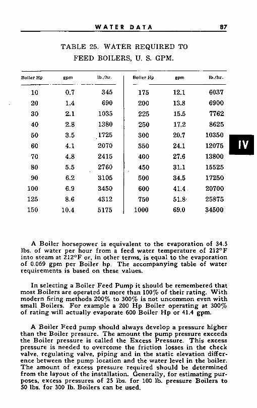
W A T E R D A T A 87
TABLE 25. WATER REQUIRED TO
F E E D BOILERS, U. S. GPM.
Boiler Hp gpm lb./hr.
10 20 30 40 50 60 70 80 90
100 125 150
0.7 345 1.4 690 2.1 1035 2.8 1380 3.5 1725 4.1 2070 4.8 2415 5.5 2760 6.2 3105 6.9 3450 8.6 4312
10.4 5175
Boiler Hp gpm lb./hr.
175 200 225 250 300 350 400 450 500 600 750
1000
12.1 6037 13.8 6900 15.5 7762 17.2 8625
31.1 15525 34.5 17250 41.4 20700 51.8. 25875 69.0 34500
A Boiler horsepower is equivalent to the evaporation of 34.5 lbs. of water per hour from a feed water temperature of 212OF into steam at 212OF or, in other terms, is equal to the evaporation of 0.069 gpm per Boiler hp. The accompanying table of water requirements is based on these values.
In selecting a Boiler Feed Pump i t should be remembered that most Boilers are operated at more than 100% of their rating. With modern firing methods 200% to 300% is not uncommon even with small Boilers. For example a 200 Hp Boiler operating at 300% of rating will actually evaporate 600 Boiler H p or 41.4 gpm.
A Boiler Feed pump should always develop a pressure higher than the Boiler pressure. The amount the pump pressure exceeds the Boiler pressure is called the Excess Pressure. This excess pressure is needed to overcome the friction losses in the check valve, regulating valve, piping and in the static elevation differ- ence between the pump location and the water level in the boiler. The amount of excess pressure required should be determined from the layout of the installation. Generally, for estimating pur- poses, excess pressures of 25 lbs. for 100 lb. pressure Boilers to 50 lbs. for 300 lb. Boilers can be used.
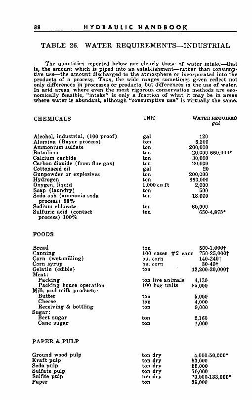
88 H Y D R A U L I C H A N D B O O K
TABLE 26. WATER REQUIREMENTS-INDUSTRIAL
The quantities reported below a r e clearly those of water intake-that is, t he amount which is piped into a n establishment-rather than consump- tive use-the amount discharged to the atmosphere or incorporated into the products of a process. Thus, the wide ranges sometimes given reflect not only differences in processes or products, but differences in the use of water. In arid areas, where even the most rigorous conservation methods are eco- nomically feasible, “intake” is only a fraction of what i t may be in areas where water is abundant, although “consumptive use” is virtually the same.
CHEMICALS
Alcohol, industrial, (100 proof) Alumina (Bayer process) Ammonium sulfate Butadiene Calcium carbide Carbon dioxide (from flue gas) Cottonseed oil Gunpowder or explosives Hydrogen Oxygen, liquid Soap (laundry) Soda ash (ammonia soda
process) 58% Sodium chlorate Sulfuric acid (contact
process) 100%
FOODS
Bread Canning Corn ( webmilling) Corn syrup Gelatin (edible) Meat:
Packing Packing house operation
Milk and milk products: Butter Cheese Receiving & bottling
Sugar : Beet sugar Cane sugar
P A P E R & P U L P
Ground wood pulp Kra f t pulp Soda pulp Sulfate pulp Sulfite pulp Paper
UNIT WATER REQUIRED gal
gal ton ton ton ton ton
ton ton
ton ton
gal
1,000 cu f t
ton ton
120 6,300
200,000 20.000-660.000* 30;OOO 20,000
20 200.000 660;OOO
2,000 500
18,000
60,000 650-4,875*
ton 500-1,OOOt
bu. corn 140-240t bu. corn 30-40t ton ’ 13,200-20,000t
100 cases #2 cans 750-25,OOOt
ton live animals 4,130 100 hog units 55,000
ton ton ton
ton ton
ton d ry ton dry ton dry ton dry ton dry ton
5,000 4,000 9,000
2,160 1,000
4,000-50,000* 93,000 85,000 70,000
39,000 70,000-133,000*
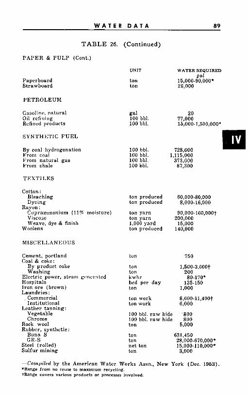
W A T E R D A T A 89
TABLE 26.
P A P E R & P U L P (Cont.)
Paperboard Strawboard
PETROLEUM
Gasolinr, natural Oil refining Refined products
SYNTHETIC F U E L
By coal hydrogenation From coal From natural gas From shale
TEXTILES
Cotton : Bleaching Dyeing
Cuprammonium (11% moisture) Viscose Weave, dye & finish
Rayon :
Woolens
MISCELLANEOUS
Cement, portland Coal & coke:
By product coke Washing
Electric power, steam gcncmted Hospitals Iron ore (brown) Laundries :
Commercial Institutional
Leather tanning: Vegetable Chrome
Rock wool Rubber, synthetic:
Buna S GR-S
Steel (rolled) Sulfur mining
(Continued)
UNIT
ton ton
gal 100 bbl. 100 bbl.
100 bbl. 100 bbl. 100 bbl. 100 bbl.
ton produced ton produced
ton yarn ton yarn 1,000 yard ton produced
ton
ton ton kwhr bed per day ton
ton work ton work
WATER REQUIRED
15,000-90,000* gal
26,000
20 77,000 15,000-1,500,000*
1,115,000 373,GOO 87,300
60,000-80,000 8,000-16,000
9O,OOO-lGO,OOO~ 200,000
15,000 140,000
750
1,500-3,600t 200 80-170*
135-150 1,000
8,600-11,400t 6,000
100 bbl. r a w hide .800 100 bbl. r a w hide 800 ton 5,000
ton 631,450 ton 28,000-670,000*
ton 3,000 net ton 15,000-110,000*
--Compiled by the American Water Works Assn., New York (Dec. 1953) *Range from no reuse to maximum recycling. tBange covers various products or processes involved.
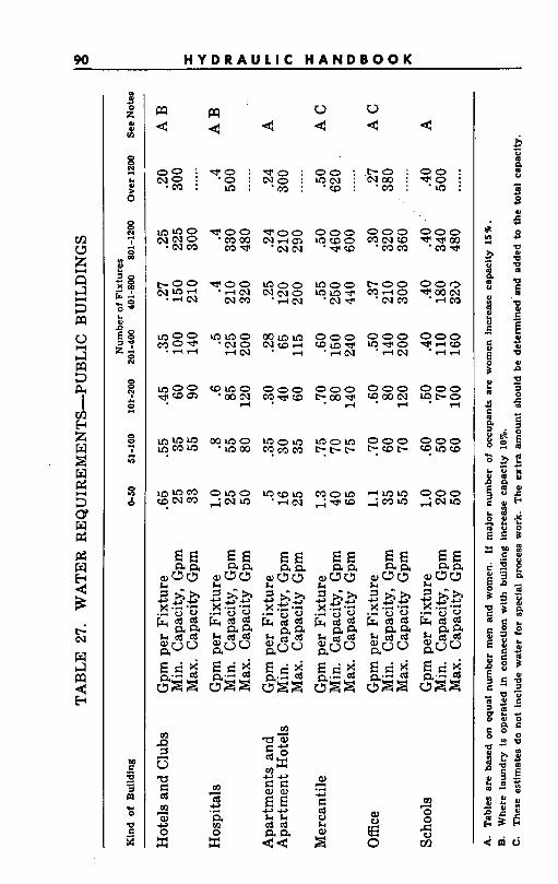
90 H Y D R A U L I C H A N D B O O K
m
B G 1
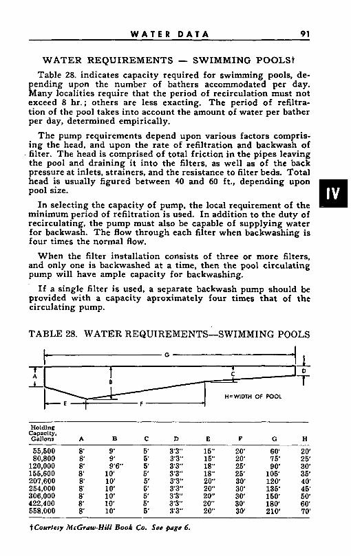
W A T E R D A T A 91
WATER REQUIREMENTS - SWIMMING POOLS+ Table 28. indicates capacity required for swimming pools, de-
pending upon the number of bathers accommodated per day. Many localities require that the period of recirculation must not exceed 8 hr.; others are less exacting. The period of refiltra- tion of the pool takes into account the amount of water per bather per day, determined empirically.
The pump requirements depend upon various factors compris- ing the head, and upon the rate of refiltration and backwash of filter. The head is comprised of total friction in the pipes leaving the pool and draining it into the filters, as well as of the back pressure at inlets, strainers, and the resistance to filter beds. Total head is usually figured between 40 and 60 ft., depending upon pool size.
In selecting the capacity of pump, the local requirement of the minimum period of refiltration is used. In addition to the duty of recirculating, the pump must also be capable of supplying water for backwash. The flow through each filter when backwashing is four times the normal flow.
When the filter installation consists of three or more filters, and only one is backwashed at a time, then the pool circulating pump will have ample capacity for backwashing.
If a single filter is used, a separate backwash pump should be provided with a capacity aproximately four times that of the circulating pump.
TABLE 28. WATER REQUIREMENTS-SWIMMING POOLS
-"-A- i C 7-
A B
HIWIDTH OF POOL
Holding Capacity, Gallons A
55,500 8' 80,800 8' 120,000 8' 155,600 8' 207,600 8' 264,000 8' 306,000 8' 422,400 8' 5 5 8,0 0 0 8'
B C
9' 5' 9' 5' 9'6' 5' 10' 5' 10 5' 10 6' 1 0 5' 10' 5' 10' 5'
D E F G
3'3'' 15" 20 6 0 3'3" 15' 20' 75' 3'3" 18' 25' 9 0 3'3" 18" 25' 106' 3'3" 20' 30' 120 3'3" 2 0 30' 135' 3'3" 20' 30' 150 3'3" 20" 30' 180 3'3 20' 30' 210'
n 20' -
~~
25' 30 35' 40' 45' 5 0 60' 70'
tCourlery McGraw-Hill Book Go. See page 6.
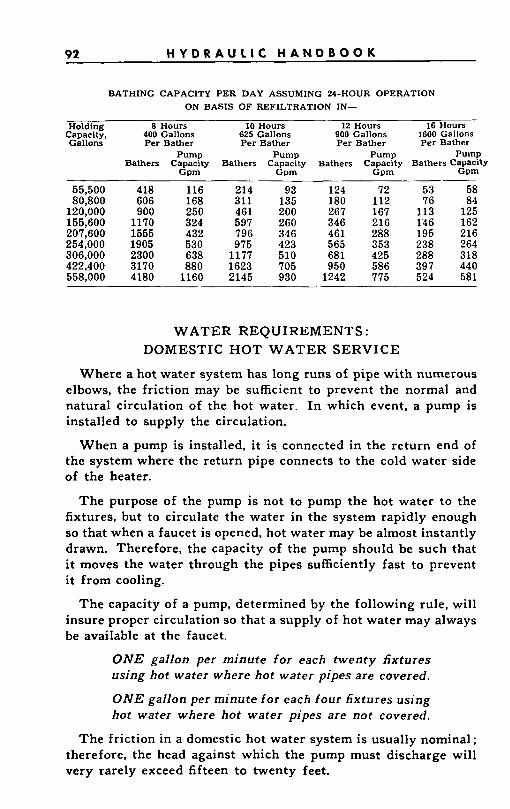
92 H Y D R A U L I C H A N D B O O K
BATHING CAPACITY PER DAY ASSUMING 24-HOUR OPERATION ON BASIS OF REFILTRATION IN-
Holding 8 Hours 10 Hours 12 Hours 16 Hours Capacity. 400 Gallons 625 Gallons 900 Gallons 1600 Gallons Gallons Per Bather Per Bather Per Bather Per Bather
Pump Pump Pump Pump Bathers Capacity Bathers Capacity Bathers Capacity Bathers Capacity
Gpm Gpm Gpm Gpm
55,500 418 116 214 93 124 72 53 58 80,800 606 168 311 135 180 112 76 84
120,000 900 250 461 200 267 167 113 125 155.600 1170 324 597 260 346 216 146 162 207;SOO 1555 432 796 346 461 288 195 216 254,000 1905 530 975 423 565 353 238 264 306.000 2300 638 1177 510 681 425 288 318 422;400 3170 880 1623 705 950 586 397 440 558,000 4180 1160 2145 930 1242 775 524 581
WATER REQUIREMENTS : DOMESTIC H O T WATER SERVICE
Where a hot water system has long runs of pipe with numerous elbows, the friction may be sufficient to prevent the normal and natural circulation of the hot water. In which event, a pump is installed to supply the circulation.
When a pump is installed, it is, connected in the return end of the system where the return pipe connects to the cold water side of the heater.
The purpose of the pump is not to pump the hot water to the fixtures, but to circulate the water in the system rapidly enough so that when a faucet is opened, hot water may be almost instantly drawn. Therefore, the capacity of the pump should be such that i t moves the water through the pipes sufficiently fast to prevent it from cooling.
The capacity of a pump, determined by the following rule, will insure proper circulation so that a supply of hot water may always be available at the faucct.
ONE gallon per minute for each twenty fixtures using hot water where hot water pipes are covered.
ONE gallon per minute f o r each four fixtures using hot water where hot water pipes are not covered.
The friction in a domestic hot water system is usually nominal; therefore, the head against which the pump must discharge will very rarely exceed fifteen to twenty feet.
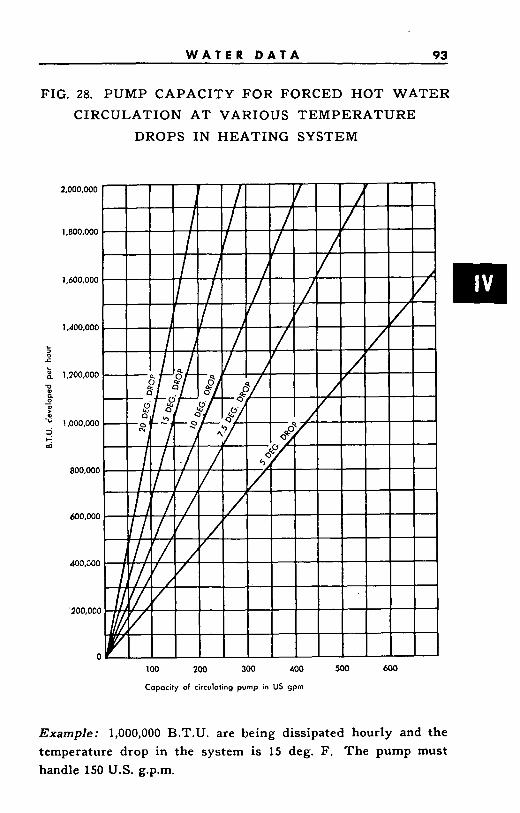
W A T E R D A T A 93
FIG. 28. PUMP CAPACITY FOR FORCED HOT WATER CIRCULATION AT VARIOUS TEMPERATURE
DROPS IN HEATING SYSTEM
100 ZOO 300 400 500 600
Capacity of circulating pump in US gpm
Example: 1,000,000 B.T.U. are being dissipated hourly and the temperature drop in the system is 15 deg. F. The pump must handle 150 U.S. g.p.m.
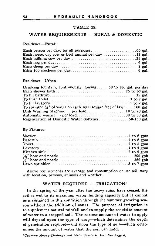
94 H Y D R A U L I C H A N D B O O K
TABLE 29.
W A T E R REQUIREMENTS - RURAL & DOMESTIC
Residence-Rural :
Each person per day, for all purposes. . . . . . . . . . . . . . . . . . . . . .60 gal. Each horse, dry cow or beef animal per day.. . . . . . . . . . . . . . . .12 gal. Each milking cow per day. . . . . . . . . . . . . . . . . . . . . . . . . . . . . . . .35 gal. Each hog per day . . . . . . . . . . . . . . . . . . . . . . . . . . . . . . . . . . . . . . . . 4 gal. Each sheep per day.. . . . . . . . . . . . . . . . . . . . . . . . . . . . . . . . . . . . . 2 gal. Each 100 chickens per day . . . . . . . . . . . . : . . . . . . . . . . . . . . . . . . . 6 gal.
Residence-Urban :
Drinking fountain, continuously flowing. . . . . .50 to 100 gal. per day Each shower bath. . . . . . . . . . . . . . . . . . . . . . . . . . . . . . . . . .25 to 60 gal. To fill bathtub . . . . . . . . . . . . . . . . . . . . . . . . . . . . . . . . . . . . . . . . . . 35 gal. To flush toilet.. . . . . . . . . . . . . . . . . . . . . . . . . . . . . . . . . . . . . . . 3 to 7 gal. To fill lavatory.. . . . . . . . . . . . . . . . . . . . . . . . . . . . . . . . . . . . . . l to 2 gal. To sprinkle M" of water on each 1000 square feet of lawn. . . .160 gal. Dish Washing Machine - per load. . . . . . . . . . . . . . . . . . .10 to 20 gal. Automatic washer - per load.. . . . . . . . . . . . . . . . . . . . . . .30 to 50 gal. Regeneration of Domestic Water Softener. . . . . . . . . . . . . . .SO-150 gal.
By Fixtures: , . .
. . . . . . . 4 to 8 gpm
. . . . 2 to 5 gpm
Toilet . . . . . . . . . . . . . . . . . . . . . . . 4 to 5 gpm Lavatory . . . . . . . . . . . . . . . . . . . . . . . . . . . . . . . . . . . . . . . . . . . 1 t o 4 gpm Kitchen sink. . . . x" hose and nozzle.. . . . . . . . . . . . . . . . . . . . . . . . . . . . . . . . . . . ,200 gph N" hose and nozzle. . . . . . . . . . . . . . . . . . . . . . . . . . . . . . . . . 360 gph Lawn sprinkler. . . . . . . . . . . .
Above requirements are average and consumption or use will vary with location, persons, animals and weather.
WATER REQUIRED - IRRIGATIONt
In the spring of the year after the heavy rains have ceased, the soil is wet to its maximum water holding capacity but it cannot be maintained in this condition through the summer growing sea- son without the addition of water. The purpose of irrigation is to supplement natural rainfall and to supply the requisite amount of water to a cropped soil. The correct amount of water to apply will depend upon the type of crop-which determines the depth of penetration required-and upon the type of soil-which deter- mines the amount of water that the soil can hold. tCourtesy Armco Drainage and Metal Products, Inc. See page 6.
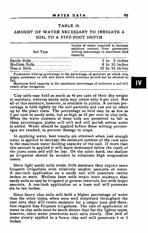
W A T E R D A T A 95
TABLE 30.
AMOUNT O F W A T E R NECESSARY T O IRRIGATE A SOIL T O A FIVE-FOOT DEPTH
Inches of water required t o increase moisture content from permanent wilting percentage to maximum field capacity.
Soil Type
Sandy Soils ..................... 3 to 5 inches
Heavy Soils .................... 12 to 15 inches Medium Soils ................... 6 to 10 inches
Permanent wilting percentage is the percentage 05 moisture at which crop plants commence to wilt and below which moisture should not be allowed to fall.
Maximum field capacity is the maximum percentage of moisture a soil will retain af ter irrigation.
Clay soils may hold as much as 40 per cent of their dyr weight in moisture, whereas sandy soils may retain only 8 per cent. Not all of this moisture, however, is available to plants. A certain per- centage is held tightly by the soil particles and can not be taken up by the plant roots. The percentage so held may be as low as 2 per cent in sandy soils, but as high as 25 per cent in clay soils. When the water contents of these soils are permitted to fall to these percentages, plants will wilt and will perish unless water is added. Water should be applied before these wilting percent- ages are reached, to prevent damage to crops.
In applying water, best results are obtained when just enough water is applied to increase the moisture content of the root zone to the maximum water holding capacity of the soil. If more than this amount is applied i t will move downward below the reach of the plant roots and will be lost. On the other hand, too shallow an irrigation should be avoided to eliminate high evaporation losses.
Since light sandy soils retain little moisture they require more frequent irrigations with relatively smaller amounts of water. A one-inch application on a sandy soil will penetrate twelve inches or more. Medium loam soils retainzmore moisture than sandy soils so may be irrigated at greater intervals, but with larger amounts. A one-inch application on a loam soil will penetrate six to ten inches.
Since heavy clay soils will hold a higher percentage of water than the other types, when once well moistened throughout the root zone they will retainfmoisture for a longer time and there- fore require less frequent irrigations. The rate of application of water to clay soils must be much slower than for the lighter types, however, since water penetrates such soils slowly. One inch of water slowly applied to a heavy clay soil will penetrate 4 or 5 inches.
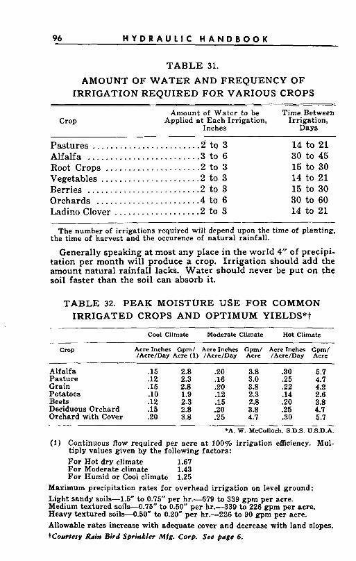
96 H Y D R A U L I C H A N D B O O K
T A B L E 31.
AMOUNT O F W A T E R AND FREQUENCY OF IRRIGATION REQUIRED FOR VARIOUS CROPS
Amount of Watcr to be Time Between Crop Applied at Each Irrigation, Irrigation,
Inches Days
Pastures ....................... . 2 to 3 14 to 21 Alfalfa ........................ . 3 to 6 30 to 45 Root Crops .................... . 2 to 3 15 to 30
14 to 21 Vegetables ..................... . 2 to 3 Berries ........................ .2 to 3 15 to 30 Orchards ...................... .4 to 6 30 to 60
14 to 21 Ladino Clover .................. . 2 to 3 -
The number of irrigations required will depend upon the time of planting, the time of harvest and the occurence of na tura l rainfall.
Generally speaking at most any place in the world 4“ of precipi- tation per month will produce a crop. Irrigation should add the amount natural rainfall lacks. Water should never be put on the soil faster than the soil can absorb it.
T A B L E 32. P E A K MOISTURE U S E F O R COMMON IRRIGATED CROPS AND OPTIMUM YIELDS*t
Cool Climate Moderate Climate Hot Climate
Crop Acre Inches Gpm/ Acre Inches Gpm/ Acre Inches Gpm/ /Acre/Day Acre (1) /Acre/Day Acre /Acre/Day Acre
Alfalfa Pasture Grain
.15 2.8 .20 3.8 .30 6.7
.12 2.3 .16 3.0 .25 4.7
.15 2.8 .20 3.8 .22 4.2 Potatoes .10 1.9 .12 2.3 .14 2.6 Beets .12 2.3 .15 2.8 .20 3.8 Deciduous Orchard .15 2.8 .20 3.8 .25 4.7 Orchard with Cover .20 3.8 .25 4.7 .30 5.7
*A. W. McCulloch. S.D.S. U.S.D.A.
(1) Continuous flow required per acre at 100% irrigation efficiency. Mul- tiply values given by the following factors: F o r Hot d ry climate 1.67 F o r Moderate climate 1.43 F o r Humid or Cool climate 1.25
Maximum precipitation rates for overhead irrigation on level ground : Light sandy soils-1.5” t o 0.75” per h r . 4 7 9 to 339 gpm per acre. Medium textured soils-0.75” to 0.50” per hr.-339 to 226 gpm per acre. Heavy textured soils--O.50“ to 0.20’’ per hr.-226 to 90 gpm per acre. Allowable rates increase with adequate cover and decrease with land slopes. tCovrtesy Rain Bird Sprinkler Mfg. Corp. See page 6.
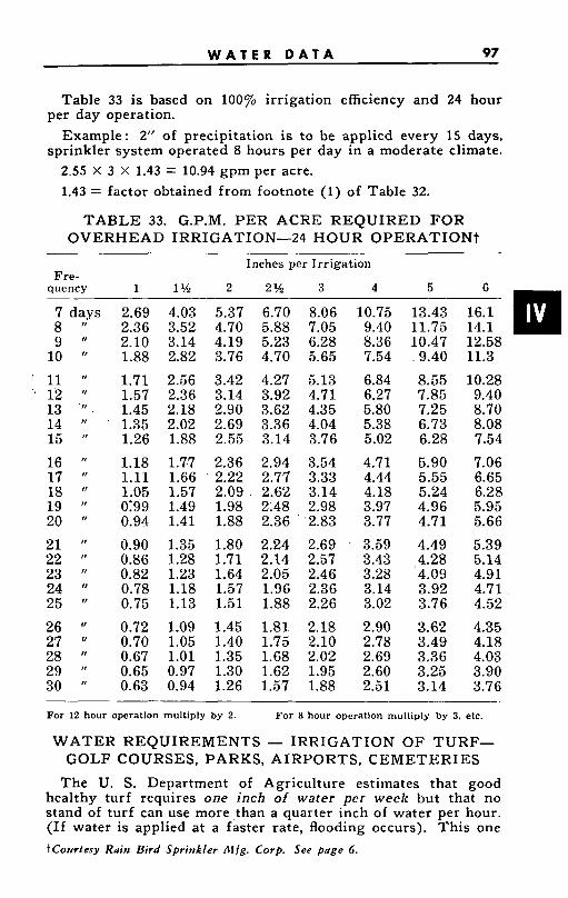
W A T E R D A T A 97
Table 33 is based on 100% irrigation efficiency and 24 hour per day operation.
Example: 2” of precipitation is to be applied every 15 days, sprinkler system operated 8 hours per day in a moderate climate.
2.55 X 3 X 1.43 = 10.94 gpm per acre. 1.43 = factor obtained from footnote (1) of Table 32.
TABLE 33. G.P.M. PER ACRE REQUIRED FOR OVERHEAD IRRIGATION-24 HOUR OPERATION?
Inches per Irrigation Fre-
7 days 8 ”
9 ”
10 If
11 ”
I 12 If
13 . “ . 1 4 ”
15 ”
16 ”
17 ”
18 “
19 ”
20
21 If
22 ”
23 ”
24 25 I’
26 27 ”
28 29 ”
30 ”
2.69 4.03 5.37 6.70 8.06 2.36 3.52 4.70 5.88 7.05 2.10 3.14 4.19 5.23 6.28 1.88 2.82 3.76 4.70 5.65
6 m quency 1 1% 2 2% 3 4 5
13.43 16.1 11.75 14.1 10.47 12.58
1.71 2.56 3.42 4.27 5.13 1.57 2.36 3.14 3.92 4.71 1.45 2.18 2.90 3.62 4.35 1.35 2.02 2.69 3.36 4.04 1.26 1.88 2.55 3.14 3.76
1.18 1.7.7. 2.36 2.94 3.54 1.11 1.66 ’ 2.22 2.77 3.33
0199 1.49 1.98 2;48 2.98 1.05 1.57 2.09 . 2.62 3.14
0.94 1.41 1.88 2.36 “2.83
0.90 1.35 1.80 2.24 2.69 0.86 1.28 1.71 2.14 2.57 0.82 1.23 1.64 2.05 2.46 0.78 1.18 1.57 1.96 2.36 0.75 1.13 1.51 1.88 2.26
0.72 1.09 1.45 1.81 2.18 0.70 1.05 1.40 1.75 2.10 0.67 1.01 1.35 1.68 2.02 0.65 0.97 1.30 1.62 1.95 0.63 0.94 1.26 1.57 1.88
10.75 9.40 8.36 7.54
6.84 6.27 5.80 5.38 5.02
4.71 4.44 4.18 3.97 3.77
3.59 3.43 3.28 3.14 3.02
2.90 2.78 2.69 2.60 2.51
9.40 11.3
8.55 10.28 7.85 9.40 7.25 8.70 6.73 8.08 6.28 7.54
5.90 7.06 5.55 6.65 5.24 6.28 4.96 5.95 4.71 5.66
4.49 5.39 ,4.28 5.14 4.09 4.91 3.92 4.71 3.76 4.52
3.62 4.35 3.49 4.18 3.36 4.03 3.25 3.90 3.14 3.76
For 12 hour operation multiply by 2. For 8 hour operation multiply by 3. etc.
WATER REQUIREMENTS - IRRIGATION O F TURF- GOLF COURSES, PARKS, AIRPORTS, CEMETERIES
The U. S. Department of Agriculture estimates that good healthy turf requires one inch of water per week but that no stand of turf can use more,than a quarter inch of water per hour. (If water is applied at a faster rate, flooding occurs). This one tCoirrfesy Rain Bird Sprinkler Aifg. Corp. See page 6.
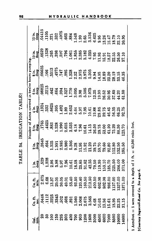
98 H Y D R A U L I C H A N D B O O K
d d d 1
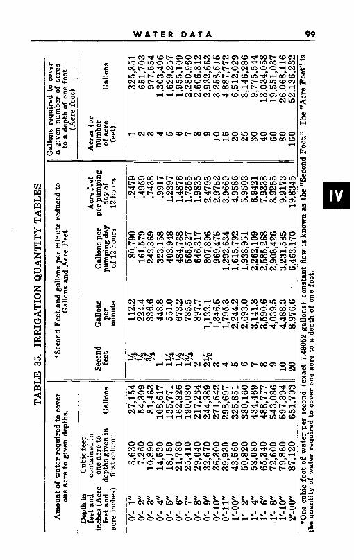
W A T E R D A T A 99
m E 0 e - d
I I
I IC%
100 H Y D R A U L I C H A N D B O O K
inch of water per week can fall in the form of rain, heavy dews, or be mechanically applied by sprinkling systems. The sprinkling system should be of ample capacity to supply sufficient water without rain or dew. One inch of water per week on an acre rep- resents 27,150 gallons of water weekly. One acre is equal to 43,560 square feet.
The best results are obtained with water at atmospheric tem- perature. For this reason, if the water supply is from a deep well, it is usually brought to the surface with deep well pumps and discharged into artificial lakes or ponds. From the lakes or ponds the water is taken by the sprinkler pump.
On the average 18 hole golf course the greens and tees are always watered an6 in the majority of cases a pump with a capacity of 150 to 175 Gpm is ample. The fairways averaging 300 yards long and approximately 60 yards wide represent 52 acres of fairway. If we figure 27,150 gallons per acre per week, the 52 acres of fairway will require approximately 1,415,000 gallons of water per week. If it is estimated that the sprinkler pumping will be done in fifty hours per week (3000 minutes) the pumping rate will be 472 Gpm. This is about the usual practice, the sprink- ling is done in a little over seven hours per night, seven nights a week. The average eighteen hole golf course requires a pump ap- proximately 500 Gpm for fairway watering.
LAND DRAINAGE - PUMPED OUTLETS Each installation must be analized before determining the pump
capacity. For preliminary estimates the following factors may be found helpful.
Multiply the land area to be drained in acres by the factor below to obtain the pump capacity in gpm:
Tile systems, subsurface drainage only-7 gpm per acre.
Surface drainage by ditch or tile, field crops-10 gpm per acre. Surface drainage by ditch or tile, truck crops-15 gpm per acre.
V I S C O U S L I Q U I D S 101
SECTION V-VISCOUS LIQUIDS
CONTENTS Page
Properties of Viscous Liquids .............................. so2
Kinematic Viscosity of Common Liquids ...................................... 103
Chart-Relation of Temperature and Viscosity .......................... 108
Chart-Temperature - Viscosity Relation of Fuel 0 3 s .. Chart-Viscosity Blending ................................................................ 110
Friction of Viscous Liquids In Pipes
109
Table-Viscosity Conversion ............................................................ 11 1
...... .............................. Friction of Viscous Liquids In Pipe Fittings 113
Chart-Relation Kinematic Viscosity and Reynolds Number .... 115
Table-Friction of Viscous Liquids In Pipes .116
Chart-Friction Loss In Pipes .......................................................... 120
Centrifugal Pump Performance When Handling Viscous Liquids ................................................................................ 121
Chart-Centrifugal Pump Performance Correction Factors ...... 124
Chart-Comparison Centrifugal Pump Perfo
Chart-Correction Chart For Viscosity and Temperature,
Viscous Liquids and Water ..........................
Reciprocating Pumps ...................................................................... 125
102 H Y D R A U L I C H A N D B O O K
SECTION V -PUMPING VISCOUS LIQUIDS
PROPERTIES O F LIQUIDS In order to solve problems involving liquids other than water,
it is essential that certain liquid properties, and their relations to each other, be understood and utilized correctly. These are spe- cific gravity, sg ; density, p (Greek letter Rho); absolute viscosity, p (Greek letter mu) ; and kinematic viscosity, Y (Greek letter nu).
SPECIFIC GRAVITY (sg) The specific gravity of a liquid is a relative term, which shows
,the fluid’s density with reference to fresh water at 39.2 deg. F, the point a t which its density is 1.0 gr. per cu. cm.
Gravity of liquids may be given in either specific gravity di- rectly, degrees Baume, degrees A P I (for oils) or Degrees Brix (for sugar) and many others, all of which are definitely related. Some of these relations are given in Section 111. DENSITY p (Greek Letter rho)
The density of a liquid is the mass per unit volume and in the English system is expressed as w/g where w is always the weight in lbs./cu. ft . and g is the acceleration caused by gravity and is taken as 32.2 ft./sec./sec., or ft./sec2. Density may also be com- puted for any liquid as follows.
Density, (p) = sg X 62.4/32.2 slugs/cu. ft. VISCOSITY
The viscosity of a liquid is a measure of the internal friction tending to resist flow. This resistance to flow, expressed as a co- efficient of absolute viscosity, is the force required to overcome the unit shear stress at a unit rate of shearing strain.
Viscosity is expressed in two ways, namely Absolute or Dy- namic viscosity, p (Greek letter mu) and Kinematic viscosity Y (Greek letter nu).
(1) The unit of Absolute viscosity in the metric system is the dyne-second per square centimeter. This unit is called a poise. The unit of Absolute viscosity in the English system has no name but is measured in pound seconds per square foot which may also be expressed as slugs per foot-second. T o convert from one system of measurement to another:
100 centipoises = 1 poise = .00209 lb. sec./ft.2 (2) Kinematic viscosity in the metric system is measured in
stokes, the unit of which is centimeters squared per second. In the English system the unit is feet ,squared per second. T o convert:
100 centistokes = 1 stoke = .00108 ft.2/sec. The above two expressions of viscosity are related for any liquid
because the Kinematic viscosity is the ratio of the Absolute vis- cosity to the density. Hence Kinematic viscosity equals p/p (mu/rho).
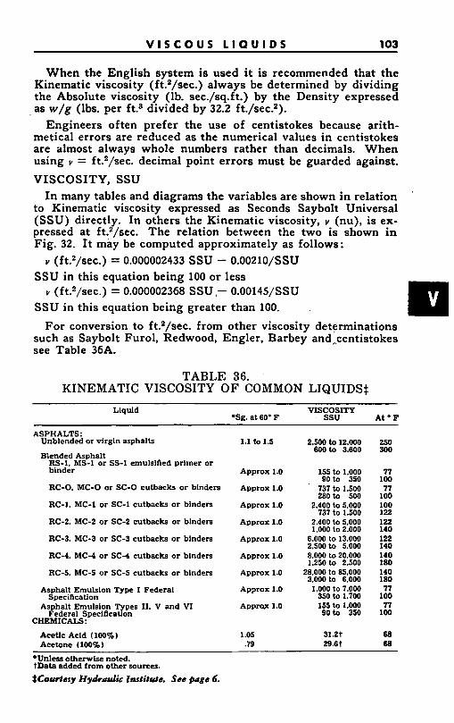
V I S C O U S L I Q U I D S 103
When the English system is used it is recommended that the Kinematic viscosity (ft.l/sec.) always be determined by dividing the Absolute viscosity (lb. sec./sq.ft.) by the Density expressed as w/g (lbs. per ft.a divided by 32.2 ft./sec.l).
Engineers often prefer the use of centistokes because arith- metical errors are reduced as the numerical values in centistokes are almost always whole numbers rather than decimals. When using v = ft.l/sec. decimal point errors must be guarded against.
VISCOSITY, SSU I n many tables and diagrams the variables are shown in relation
to Kinematic viscosity expressed as Seconds Saybolt Universal (SSU) directly. In others the Kinematic viscosity, v (nu), is ex- pressed at ft.2/sec. The relation between the two is shown in Fig. 32. I t may be computed approximately as follows:
v (ft.l/sec.) = 0.000002433 SSU - O.O021O/SSU SSU in this equation being 100 or less
v (ft.2/sec.) = 0.000002368 SSU ,- O.O0145/SSU SSU in this equation being greater than 100.
For conversion to ft.2/sec. from other viscosity determinations such as Saybolt Furol, Redwood, Engler, Barbey and,centistokes see Table 36A.
TABLE 36. KINEMATIC VISCOSITY O F COMMON LIQUIDS+
Liquid VISCOSITY *Sg. at 60" F - ssu At F
ASPHALTS: Unblended or virgin asphalts
B:ended Asphalt RS-1. MS-1 or SS-1 emulsified primer or binder
RC-0. MC-0 or SC-0 cutbacks or binders
RC-1. MC-1 or SC-1 cutbacks or binders
RC-2. MC-2 or SC-2 cutbacks or blnders
RC-3. MC-3 or SC-3 cutbacks or blnders
RC-4. MC-4 or SC-4 cutbacks or binders
RC-5. MC-5 or SC-5 cutbacks or binders
Asphalt Emulsion Type I Federal Specification
Asphalt Emulsion Types 11. V and VI Federal Specificauon
CHEMICALS :
Acetlc Acid f 100%) Acetone (100%)
1.1 to 1.5
Approx 1.0
Approx 1.0
Approx 1.0
Approx 1.0
Approx 1.0
Approx 1.0
Appmx 1.0
Aparox 1.0
Apprax 1.0
1 .05 .79
2.500 to 12.000 600to 3,600
155 to 1,000 goto 350
737 to 1.500 28Oto 500
2.400 to 5.000 737 to 1.500
2,400 to 5.000 1,000 to 2.000
6.000 to 13.000 2,500 to 5.000 8,000 to 20.000 1.250 to 2.500
28,000 to 85,000 3.000 to 6.000
1,000 to 7.000 350 to 1.700 155 to 1.000 9oto 350
31.2t 29.6t
250 300
71 100 77
100 100 122 122 140 122 140 140 180 140 180 17
100 77
100
68 68
*Unles3 otherwise noted. tData added from other sources.
#Com&sy Hydrovlic Insti1ds. See page 6.
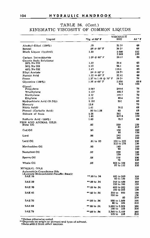
104 H Y D R A U L I C H A N D B O O K
TABLE 36. (Cont.) KINEMATIC VISCOSITY O F COMMON LIQUIDS
Liquid
Alcohol-Ethyl (100%) Benzol Black Liquor (typical)
Carbon Tetrachloride Caustic Soda Solutions:
20% Na OH 30% Na OH 40% Na OH
Ethyl Acetate Formic Acid Freon Glycerine (100%)
Glycol: Propylene Triethylene Diethylene Ethylene
Hydrochloric Acid (31.5%) Mercury Nitric Acidt Phenol (Carbolic Acid) Silicate of Soda
Sulfuric Acid (100% I FISH AND ANIMAL OILS:
Bone Oil
Cod Oil
Lard
Lard Oil
Menhadden Oil
Neatsfoot Oil
Sperm Oil
Whale Oil
MINERAL OILS Automobile Cranckcase Oils (Average Midcontinent Paraffin Base):
SAE 10
SAE 20
SAE 30
SAE 40
SAE 50
SAE 60
SAE 70
VISCOSITY *Sg. at 60" F ssu At F
.79
.88 @ 68' F 1.30
1.59 @ 68" F
1.22 1.33 1.43 .90 @ 68" F
1.22 @ 68'F 1.37 to 1.49 @ 70' 1.26 @ 68" F
1.04t 1.13t 1.12 1.13 1.15t 13.6 1.41
1.38 1.41 1.83
.92
.93
.96
.91 to .93
.93
.92
.88
.93
.95 to 1.08
**.88 to .94
**.88 to .94
**.88 to .94
**.88 to .94
**.88 to .94
**A8 to .94
**.as to .94
32 3t 30 3t 5.000 2.500 30.1 t
39.4 58.1
110.1 29.7t 32.47
F 29.3t 2.950
813
240.6 185.7 149.7 88.4 33t
31.5 65
365 637.6 75.7
220 65
150 95
2R7 160
190 to 220 112 to 128
140 90
230 130 110 78
163 to 184 97 to 112
165 to 240 90 to 120
240 to 400 120 to 185 400 to 580 185 to 255
580to 950 255 to
80 950 to 1.600 80 to 105
1,600 to 2.300 105to 125
2,300 to 3.100 125 to 150
68 68
122 130 68
65 65 65 68 68 70 68.6
100
70 70 70 70 68 70 68 65
100 100 68
130 212 100 130 100 130 100 130 100 130 100 130 100 130 100 130
100 130 100
100 130 100 130 210 100 210 100 210 100 210
130
*Unless otherwise noted.
tData added from other sources. **Depends a n origin or percent and type of solvent.
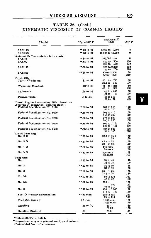
V I S C O U S L l O U l D S 105
TABLE 36. (Cont.) KINEMATIC VISCOSITY O F COMMON LIQUIDS
VISCOSITY Liquid *Sg. at 60' F ssu At F
SAE 1OW SAE 2OW
SAE 80 SAE 90
SAE 140
SAE 250
Crude Oils:
Automobile Transmission Lubricants:
Texas. Oklahoma
Wyoming. Montana
California
Pennsylvania
Diesel Engine Lubricating Oils (Based on Average Mldcontinent Paraffin Base):
Federal Specification No. 9110
Federal Specification No. 9170
Federal Specification No. 9250
Federal Specification No. 9370
Federal Specification No. 9500
Diesel Fuel Oils: No. 2 D
No. 3 D
No. 4 D
No. 5 D
Fuel Oils: No. 1
No. 2
No. 3
No. SA
No. 5B
No. 6
Fuel Oil-Navy specification
Fuel Oil-Navy XI
Gasoline
Gasoline (Natural)
*Unless otherwise noted.
tData added from other sources. **Depends on origin or percent and type of solvent.
* * .E8 to .94 ".88 to .94
'"3 to .94 **.E8 to .94
**.88 to .94
99.88 to .94
.81 to .92
.86 to .88
.78 to .92
.8 to .85
".88 to .94
09.88 to .94
**.E8 to .94
**.88 to .94
*9.m to .94
**.82 to .95
**.82 to .95
**.a2 to .95
**.82 to .95
**.82 to .95
**.82 to .95
**.82 to .95
*'.82 to .95
**.82 to .95
**.a2 to .95
**.99 max
1.0 max
.68 to .74
.68
5.000 to 10.000 lO.000 to 40.000
100,000 max 800 to 1,500 300 to 500 950 to 2.300 120 to 200 Over 2.300 Over 200
40 to 783 34.2 to 210 74 to 1.215 46 to 320 40 to 4.840 34 to 700 46 to 216 38to 86
165 to 240 90 to 120 300 to 410 140 to 180 470 to 590 200 to 255 800 to 1,100 320 to 430 490 to 600 92 to 105
32.6 to 45.5 39
45.5 to 65 39 to 48 140 max 70 max
400 max 165 max
34 to 40 32 to 35 36 to 50 33 to 40
35 to45 32.8 to 39 50 to 125 42 to 72 125 to
dnn 72 to ii6
450 to 3.000 175 to 780 110 l o 225 63 to 115 1.500 max 480 max 30 t 29.9t 29.6t
0 0
0 100 130 130 210 130 210
60 100 60 100 60
100 130 100 130 100 130 100 130 130 210
100 130 100 130 100 130 122 160
70 100 70 100 100 130 100 130 100 122 130 122 160 122 160 122 160 60 100 68
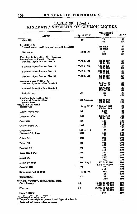
106 H Y D R A U L I C H A N D B O O K
TABLE 36. (Cont.) KINEMATIC VISCOSITY OF COMMON LIQUIDS
VISCOSITY Ltquld *Sg. at 60" B ssu At'F
cas Oil as Insulating Oil:
Transformer, switches and circuit breakers
Kerosene
Machine Lubricatin 011 (Average Pennsylvania ParaAn B-) :
Federal Specification No. 8
Federal Specification- No. 10
Federal Specification No. 20
Federal Specification No. 30
Mineral Lard Cutting Oil: Federal Specification Grade 1
Federal Specification Grade 2
Petrolatum
Turbine Lubrlcatin Oll: Federal SpecUlCa%oion (Perm Base)
VEGETABLE O m : Castor 011
Chlna Wood 011
cocoanut oll Corn Oil
Cotton Seed oil
Creosotet Ltnseed 011. Raw
Olive 011
Palm Oil
Peanut 011
Rape seed Oil
Rosin 011
Rosin (Wood)
Sesame 011
Soja Bean Oil (Soya)
Turpentine
SUGAR SYRUF'S. MOLASSES. ETC. Corn Syrups
Glucose
.7a to .LIZ
**as to .94
**.a8 to .94
**.a to .94
**.sa to .94
63
91 Average
.96@6888'F
.s4
mt .92
st
1.04 to 1.10 mt a t
.a 92
.92
.on 1.09 (A%%.)
92
.93 to .sa d?
1.5
1.4
73 50
115 max amax 35 32.6
I12 to 160 70to 90 16Oto235
90 to 120 235to385 120 to 185 w t o 5 5 0 lSSto255
140 to 190 86 to 110 190 to 220 110 to 125
100 TI
400 to 440 185 to 205
1.200 to 1.500 450to 600
1,425 580
140 to 148 76to 80
70 143 s3
200 115 221 125 195 112 250 I45
1.500 600
110 165 gs 33 32.6
5.000 to 500.ooo 1.500to 60.000
55.000 to 100.OOo &to 11.Ooo
70 100
70 100 68
100
100 130 100 130 100 130 100 150
100 130 100 130 150 160
100 130
100 130 09
100 100 130 130 212 100 130 68
100 130 100 130 IC@ 130 100 130 100 130 100 130 200 130 100 130 100 130 60
100
100 130 100 150
Honey (Raw) 340 100
.Unless otherwlse noted.
tData added from other sourcea. **Depends on origin or percent and type of solvent.
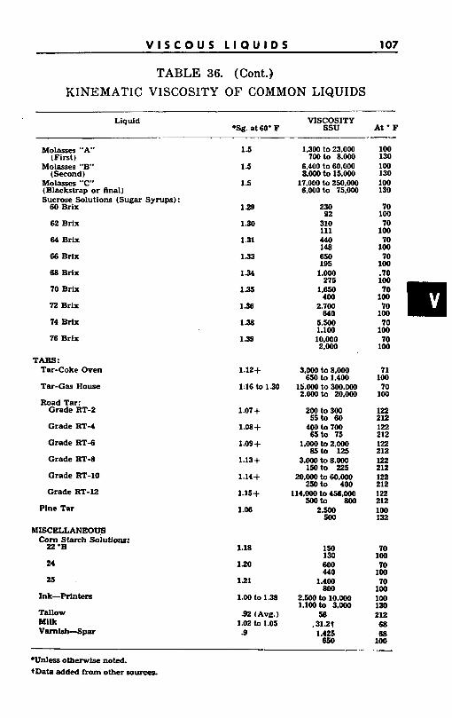
V I S C O U S L l O U l D S 107
TABLE 36. (Cont.) KINEMATIC VISCOSITY O F COMMON LIQUIDS
Liquld VISCOSITY *Sg. at 60’ F ssu At - F
Molasses “A” (First)
Molasses “E’ (Second )
Molasses “C” (Blackstrap or Anal) Sucrose Solutions (Sugar Syrups):
60 Brix
62 Brix
64 Brix
66 Brix
68 Brix
IO Brlx
I2 Brix
14 Brix
16 Brix
TARS: Tar-Coke Oven
Tar-Gas HOW
Road Tar: Grade RT-2
Grade RT-4
Grade RT-6
Grade RT-8
Grade RT-10
Grade RT-12
Plne Tar
MISCELLANEOUS Starth &8lUtlOnS:
22 ‘B
24
25
Ink-PrlIlteln
Tallow Mllk VtUlliSh--Spar
1.5
1.5
1.5
1.29
1 .so 1.31
1.33
1.34
1.35
1 s
138
139
1.12+
1:16 to 1.30
1.07 + l.Oa+
1.09+
1.13+
1.14+
1.15+
1.06
1.18
120
121
1.00 to 1.38
92 (Avg.) 1.02 to 1.05 9
1.300 to 23.000 100 to 8.000
6,400 to 60.000 1.000 to 15.000
17.000 to 250,000 6.000to 15.000
230 92
310 111 440 148 650 195
1.000 215
1.650 400
2.700 640
5.500 1.100 10.000 2.000
3.000 to 8.000 650 to 1.400
1s.OOo to 300.000 2.000to 20.000
200 to 300 55to 60
400 to I00 65to 75
1.000 to 2.000 85to 125
3.000 to 8.000 150to 225
20.000 to 6o.OOo 250to 400
114.000 to 456.000 soot0 800
2.500 500
150 130 600 440
1.400 800
2.500 to 1o.OOo 1.100 to 3.000
56 .312t 1.425 650
100 130 100 130 100 130
IO 100 70
100 IO
100 IO
100 .70
IO 100 IO m 100 IO
100
11 100 70
100
122 212 122 212 122 212 122 212 122 212 122 212 100 132
70 100 10
100 10
100 100 130 212 68 68
100
*Unless otherwfse noted. tData added from other soureea
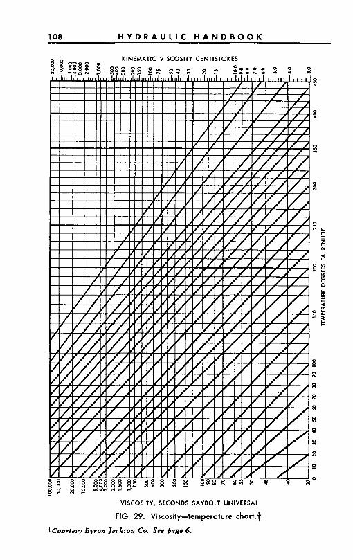
108 H Y D R A U L I C H A N D B O O K
KINEMATIC VISCOSITY CENTISTOKES
5:
8
5: o
8 o
0
" C w I Z
I 4
w LI
L
WE LI
0
Iy p: 3 I-
4 LI o w
e
' 3 I-
s s. 0 - 0 h
3 0 0
0 0
:: s!
0
VISCOSITY, SECONDS SAYBOLT UNIVERSAL
FIG. 29. Viscosity-temperature ch9rt.t
+Courtesy Byron Jackson Co. See page 6.
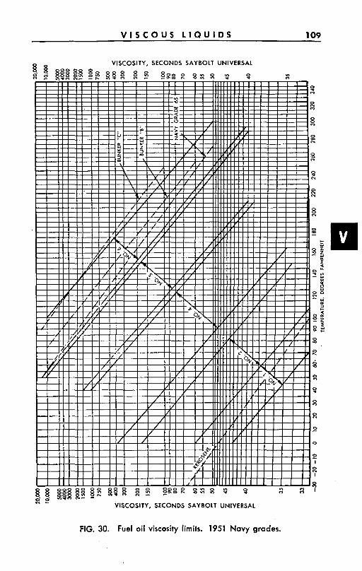
V I S C O U S L I Q U I D S 109
VISCOSITY, SECONDS SAYBOLT UNIVERSAL 8 9 @ g $ $ $ 2 3 g 5 g g g z 3 $ 3 v)
g g 88883 $ 5 8 8 5 5 5 2 s E 8 2 SL 7 8 F : P
VISCOSITY, SECONDS SAYBOLT UNIVERSAL
FIG. 30. Fuel oil viscosity limits. 1951 Navy grades.
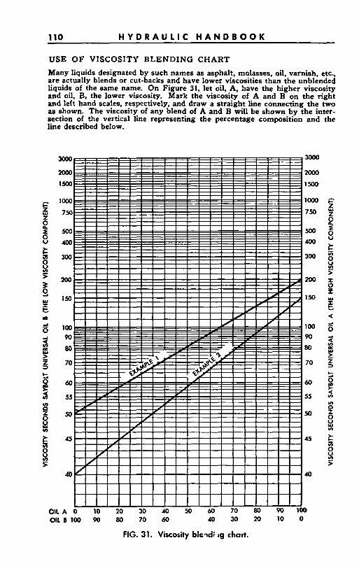
110 H Y D R A U L I C H A N D B O O K
USE OF VISCOSITY BLENDING CHART
Many liquids designated by such names as asphalt, molasses, oil, varnish, etc., are actually blends or cut-backs and have lower viscosities than the unblended liquids of the same name. On Figure 31, let oil, A, Save the higher viscosity and oil, B, the lower viscosity. Mark the viscosity of A and B on the right and left hand scales, respectively, and draw a straight line connecting the two as shown. The viscosity of any blend of A and B will be shown by the inter- section of the vertical line representing the percentage composition and the line described below.
011 B 100 90 80 70 60 4 0 3 0 2 0 1 0 0
FIG. 31. Viscosity bleqdi ig chart.
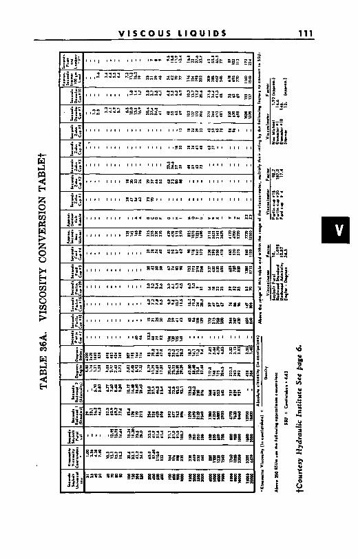
V I S C O U S L I Q U I D S 111
* -I I".
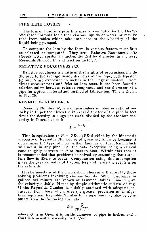
112 H Y D R A U L I C H A N D B O O K
PIPE L I N E LOSSES
The loss of head in a pipe line may be computed by the Darcy- Weisbach formula for either viscous liquids or water, or may be read from tables which take into account the viscosity of the liquid being pumped.
T o compute the loss by the formula various factors must first be selected or computed. They are: Relative Roughness, c / D (Greek letter epsilon in inches divided by diameter in inches); Reynolds Number R ; and friction factor, f.
RELATIVE ROUGHNESS r /D.
Relative roughness is a ratio of the heights of protrusions inside the pipe to the average inside diameter of the pipe, both Epsilon (e ) and D are expressed in inches in the English system. From direct measurement and friction loss tests, it has been found a relation exists between relative roughness and the diameter of a pipe for a given material and method of fabrication. This is shown in Fig. 26.
REYNOLDS NUMBER, R. Reynolds Number, R, is a dimensionless number or ratio of ve-
locity in f t . per sec. times the internal diameter of the pipe in feet times the density in slugs per cu.ft. divided by the absolute vis- cosity in lbsec. per sq.ft.
V D Y
R = . - ? -
This is equivalent to R = VD,/ ,> ( V D divided by,the kinematic viscosity). Reynolds Number is of great significance because it determines the type of flow, either laminar or turbulent, which will occur in any pipe line, the only exception being a critical zone roughly between an R of 2000 to 3500. Within this zone it is recommended that problems be solved by assuming that turbu- lent flow is likely to occur. Computation using this assumption gives the greatest value of friction loss and hence the result is on the safe side.
It is believed use of the charts shown herein will appeal to those solving problems involving viscous liquids. When discharge in gallons per minute are known or assumed, tables 1 and 2 give the velocity quickly. Hence by simple arithmetic and use of Fig. 32 the Reynolds Number is quickly obtained with adequate ac- curacy. For those who prefer the greater precision of an alge- braic equation, Reynolds Numbei for a pipe line may also be com- puted from the following formula:
Q 29.4 -d-v-
R =
where Q is in Gpm. d is inside diameter of pipe in inches, and v (nu) is kinematic viscosity in ft.'/sec.
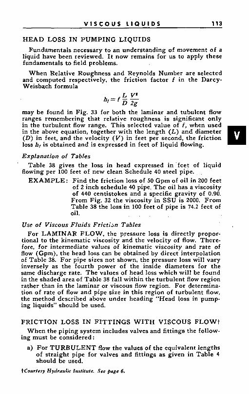
V I S C O U S L l O U l D S 113
HEAD LOSS IN PUMPING LIQUIDS
Fundamentals necessary to an understanding of movement of a liquid have been reviewed. It now remains for us to apply these fundamentals to field problems.
When Relative Roughness and Reynolds Number are selected and computed respectively, the friction factor f in the Darcy- Weisbach formula
L V’ h - f - - I - D 2 g
may be found in Fig. 33 for both the laminar and tubulent flow ranges remembering that relative roughness is significant only in the turbulent flow range. This selected value of f, when used in the above equation, together with the length (L) and diameter (D) in feet, and the velocity (V) in feet per second, the friction loss h, is obtained and is expressed in feet of liquid flowing.
Explanation of Tables
flowing per 100 feet of new clean Schedule 40 steel pipe., .
’ Table 38 gives the loss in head expressed in ‘feet of liquid
EXAMPLE: Find the friction loss of 50 Gpm of oil in 200 feet of 2 inch schedule 40 pipe. The oil has a viscosity of 440 centistokes and a specific gravity of 0.90. From Fig. 32 the viscosity in SSU is 2000. From Table 38 the loss in 100 feet of pipe is 74.2 feet of oil. . . .
Use of Viscous Fluids Frictizn Tables For LAMINAR FLOW, the pressure loss is directly propor-
tional to the kinematic viscosity and the velocity of flow. There- fore, for intermediate values of kinematic viscosity and rate of flow (Gpm), the head loss can be obtained by direct interpolation of Table 38. For pipe sizes not shown, the pressure loss will vary inversely as the fourth power of the inside diameters for the same discharge rate. The values of head loss which will be found in the shaded area of Table 38 fall within the turbulent flow region rather than in the laminar or viscous flow region. For determina- tion of rate of flow and pipe size in this region of turbulent flow, the method described above under heading “Head loss in pump- ing liquids” should be used.
FRICTION LOSS I N FITTINGS W I T H VISCOUS F L O W t When the piping system includes valves and fittings the follow-
ing must be considered:
a) For TURBULENT flow the values of the equivalent lengths of straight pipe for valves and fittings as given in Table 4 should be used.
t Courlesy Hydraulic Institule. See page 6,
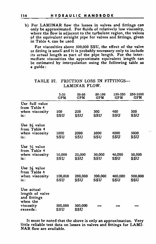
114 H Y D R A U L I C H A N D B O O K
b) For LAMINAR flow the losses in valves and fittings can only be approximated. For fluids of relatively low viscosity, where the flow is adjacent to the turbulent region, the values of the equivalent straight pipe for valves and fittings, given in Table 4, can be used.
For viscosities above 500,000 SSU, the effect of the valve or fitting is small and i t is probably necessary only to include its actual length as part of the pipe length. For the inter- mediate viscosities the approximate equivalent length can be estimated by interpolation using the following table as a guide:
TABLE 37. FRICTION LOSS I N FITTINGS- LAMINAR FLOW.
3-30 30-50 50-100 100-260 250-1000 GPM GPM GPM GPM GPM
~ ~~
Useful l value from Table 4 when viscosity is :
Use 3/s value from Table 4 when viscosity is :
Use % value from Table 4 when viscosity is :
Use % value from Table 4 when viscosity is :
Use actual length of valve and fittings when the viscosity exceeds :
100 200 300 400 ssu ssu ssu ssu
1000 2000 3000 4000 ssu ssu ssu ssu
10.000 20.000 30,000 40,000 ssu ssu ssu ssu
100,000 200,000 300,000 400,000 ssu ssu ssu ssu
500.000 500,000 - - ssu ssu
500 ssu
5000 ssu
50,000 ssu
500,000 ssu
It must be noted that the above is only an approximation. Very little reliable test data on losses in valves and fittings for LAMI- NAR flow are available.
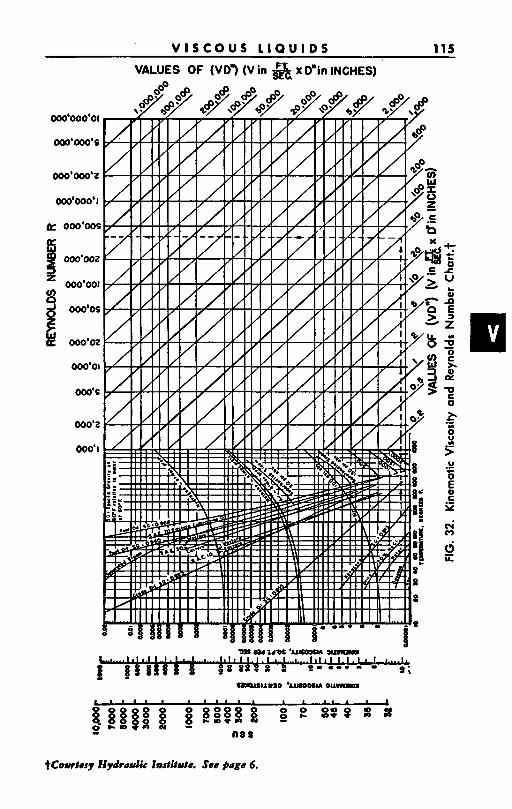
V I S C O U S L I Q U I D S 115
oO0'000'0l
000'000.S
000'000'2
oO0'00O'l
b: 000'00s
~ 0 0 0 ' 0 0 2
000'001
8 d ooo'oc
ii oO0'02
OOo'Ol
000's
000'2
000' I
~~
VALUES OF (VD? (V in gG x d i n INCHES)
tCourlesy Hydrawk Zartirvk See poge 6.
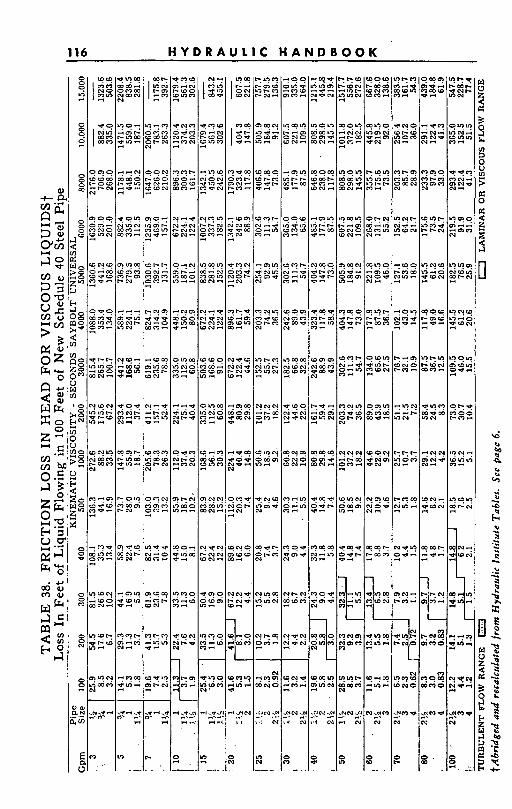
116 - H Y D R A U L I C H A N D B O O K
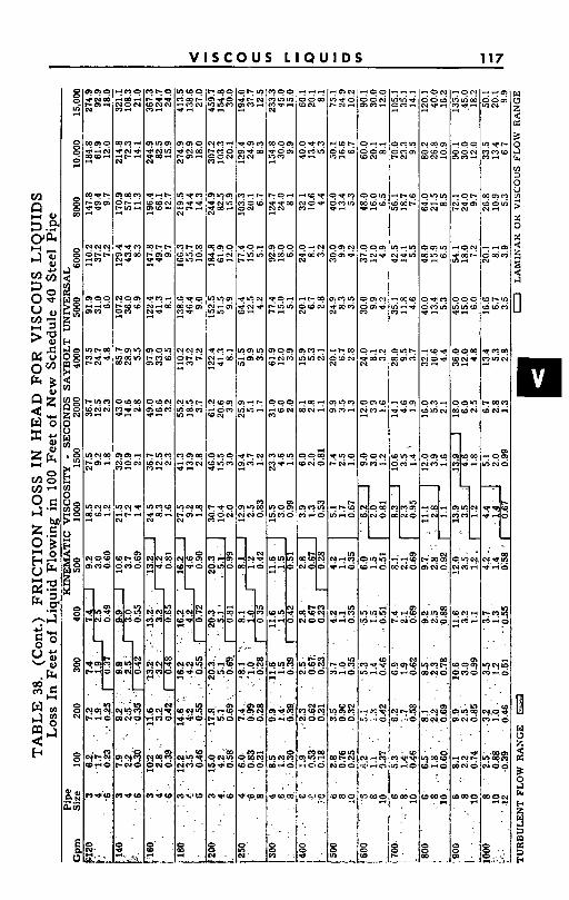
V I S C O U S L I Q U I D S 117
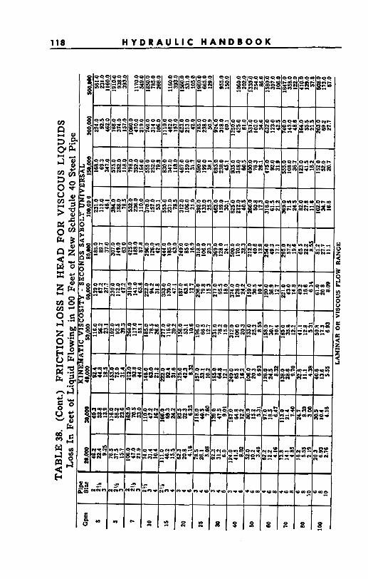
118 H Y D R A U L I C H A N D B O O K
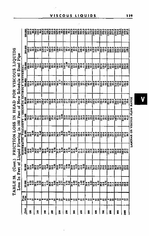
V I S C O U S L I Q U I D S 119
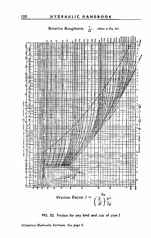
120 H Y D R A U L I C H A N D B O O K
Relative Roughness -'- (Refer to Fig. 26) D
hF Friction Factor f = z , ~
FIG. 33. Friction for any kind and size of pipe.t
$Courtesy Hydraulic Institute. See page 6.
V I S C O U S L I Q U I D S 121
CENTRIFUGAL PUMP PERFORMANCE W H E N HANDLING VISCOUS LIQUIDSt
It is recognized that the performance of centrifugal pumps is affected when handling viscous liquids. The effects are a marked increase in brake horsepower, a reduction in head, and some re- duction in capacity a t moderate and high viscosities.
It is the purpose of Fig. 34A and 34B, to provide a means of deter- mining the performance of a conventional design of centrifugal pump handling a viscous liquid, when its performance on water is known. It is also intended to be used, by an approximate method, as an aid in selecting a pump for a given application. The cor- rections are based on tests of conventional single stage pumps of 2" to S'l size, handling petroleum oils. The correction curves are an average for several pumps and are, therefore, not exact for a particular pump. It is suggested that performance tests using the viscous liquids be conducted whenever facilities are available for an accurate test.
LIMITATIONS F O R USE Use only within the scales shown. DO NOT extrapolate. Use only for pumps of conventional hydraulic design, in the normal operating range with open or closed impellers. DO N O T use for mixed flow or axial flow pumps or for pumps of special hydraulic design for either viscous or non-uniform liquids. Use only where adequate NPSH is available in order to avoid the effect of cavitation. Use only on Newtonian (uniform) liquids. Gels and slur- ries, paper stock, and other non-uniform liquids may pro- duce widely varying results, depending on the particular characteristics of the liquid.
INSTRUCTIONS F O R PRELIMINARY SELECTION OF A
DITION. Given the desired capacity and head of the viscous liquid to
be pumped and the viscosity and specific gravity at the pumping temperature, enter Fig. 34A & B a t the bottom with the desired vis- cous capacity, (euis) and proceed upward to the desired viscous head (Hvis) in feet of liquid. For multistage pumps, use head per stage. Proceed horizontally (either left or right) to the fluid viscosity, and then go upward to the correction curves. Di- vide the viscous capacity (eurs) by the capacity correction factor (C,) to get the approximate equivalent water capacity (ew ap- prox.). Divide the viscous head (Hui8) by the head correction factor (C,) from the curve marked "1.0 X en'' to get the approxi- mate equivalent water head (H, approx.). Using this new equiva- lent water head-capacity point, select a pump in the usual manner.
PUMP FOR GIVEN HEAD-CAPACITY-VISCOSITY CON-
tCourtesy Hydraulic Institute. See page 6.
122 H Y D R A U L I C H A N D B O O K
The viscous efficiency and the viscous brake horsepower may then be calculated.
This procedure is approximate as the scales for capacity and head on the lower half of Fig. 34 A 8a B are based on the water per- formance. However, the procedure has sufficient accuracy for most pump selection purposes.
Example Requirement: a pump to deliver 750 Gpm of oiI a t 100 feet total
head of liquid having a viscosity of 1000 SSU and a specific gravity of 0.90 at the pumping temperature.
Enter Fig. 34B with 750 Gpm, go up to 100 feet head, over to 1000 SSU, and then up to the correction factors:
CQ = 0.95 cli = 0.92 (for 1.0 en) CE = 0.635
750 0.95 Q w = - - 7 9 0 Gpm H,=- loo - - 108.8 say 109 feet head
0.92
Select a pump for a water capacity of 790 Gpm at 109 feet head. The selection should be at or close to the maximum efficiency point for water performance. If the pump selected has an effici- ency on water of 81% at 790 Gpm, the efficiency for the viscous liquid will be as follows: EVk = 0.635 X81% = 51.5%
The brake horsepower for pumping the viscous liquid is
750 X 100 X 0.90 = 33.1 hp = 3960 X 0.515
For performance curves of the pump selected, correct the water performance as shown in the following paragraphs.
ANCE ON A VISCOUS LIQUID W H E N PERFORMANCE ON WATER IS KNOWN.
Given the complete performance characteristics of a pump handling water to determine the performance when pumping a liquid of a specified viscosity.
From the efficiency curve, locate the water capacity (1.0 Qn) at which maximum efficiency is obtained. From this capacity, de- termine the capacities 0.6 X Qn, 0.8 X Qn and 1.2 Qn. Enter the chart a t the bottom with the capacity a t best efficiency (1.0 en), go upward to the head developed (in one stage) (H,,,) at this ca- pacity, then horizontally (either left or right) to the desired vis- cosity, and then proceed upward to the various correction curves. Read the values of Cg and CQ, and of CH for all four capacities. Multiply each capacity by CQ to obtain the corrected capacities. Multiply each head by its corresponding head correction factor to obtain the corrected heads. Multiply each efficiency value by Cg to obtain the corrected efficiency values, which apply at the corresponding corrected capacities.
INSTRUCTIONS FOR DETERMINING PUMP PERFORM-
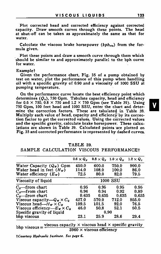
V I S C O U S L I Q U I D S 123
Plot corrected head and corrected efficiency against corrected capacity. Draw smooth curves through these points. The head at shut-off can be taken as approximately the same as that for water.
Calculate the viscous brake horsepower (bphVb) from the for- mula given.
Plot these points and draw a smooth curve through them which should be similar to and approximately parallel to the bph curve for water.
Examplet Given the performance chart, Fig. 35 of a pump obtained by
test on water, plot the performance of this pump when handling oil with a specific gravity of 0.90 and a viscosity of 1000 SSU at pumping temperature.
On the performance curve locate the best efficiency point which determines ( Qn), 750 Gpm. Tabulate capacity, head and efficiency for 0.6 X 750, 0.8 X 750 and 1.2 X 750 Gpm (see Table 39). Using 750 Gpm, 100 feet head and 1000 SSU, enter the chart and deter- mine the correction factors. These are tabulated in Table 39. Multiply each value of head, capacity and efficiency by its correc- tion factor to get the corrected values. Using the corrected values and the specific gravity, calculate brake horsepower. These calcu- lations are shown in Table 39. Calculated points 'are plotted on Fig. 35 and corrected performance is represented by dashed curves.
TABLE 39. SAMPLE CALCULATION VISCOUS PERFORMANCE+
Water Capacity (Qw) Gpm 450.0 600.0 750.0 900.0 Water head in feet ( H , ) 114.0 108.0 100.0 86.0 Water efficiency (Ew) 72.5 80.0 82.0 79.5 Viscosity of liquid 1000 ssu CQ-from chart 0.95 0.95 0.95 0.95 C-from chart 0.96 0.94 0.92 0.89 C-from chart 0.635 0.635 0.635 0.635 Viscous capacity-Q, X C4 427.0 570.0 712.0 855.0 Viscous head-I-l, x CH 109.5 101.5 92.0 76.5 Viscous efficiency--Ew x Ce 46.0 50.8 52.1 50.5
bhp viscous 23.1 25.9 28.6 29.4
bhp viscous =
Specific gravity of liquid 0.90
viscous capacity x viscous head x specific gravity 3960 x viscous efficiency
tCowtesy Hydraulic Institute. See puge 6.
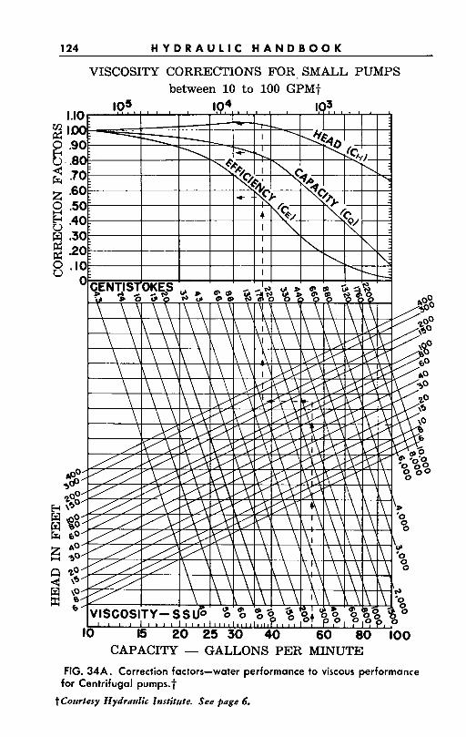
124 H Y D R A U L I C H A N D B O O K
VISCOSITY CORRECTIONS FOR. SMALL PUMPS between 10 to 100 GPMt
CAPACITY - GALLONS PER MINUTE FIG. 34A. Correction factors-water performance to viscous performance
for Centrifugal pumps.t
t Corrrtesy Hydraulic Institute. See page 6.
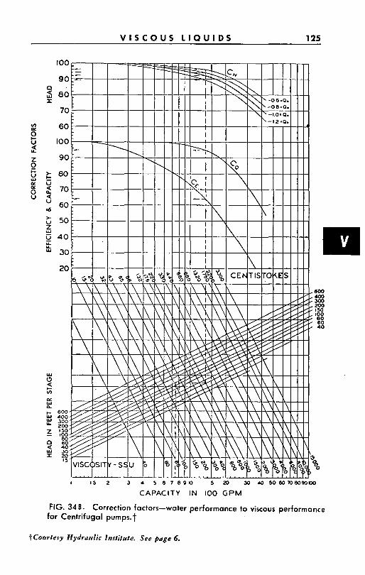
V I S C O U S L I Q U I D S 125
0 a w r
In a
g a P X k
LL
Z
+ * I Y U
2 4 .d > U Z w I! Y Y w
? I- In
m w Q
I- w w U
z n a r w
100
90
80
70
60
100
90
80
70
60
50
40
30
20
600 400 300 200 I50 100 80 60 40 30 20 I5
I 2 3 15 4 5 e 7 8 0 IQOW
CAPACITY IN I00 GPM
FIG. 34 B. Correction factors-water performance to viscous performance for Centrifugal pumps.t
t Courtesy Hydrarrlic lnstitrrte. See #age 6.
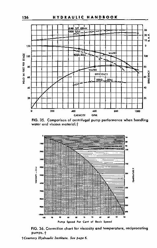
126 H Y D R A U L I C H A N D B O O K
30
f 10 d
120 0
2 100 100
t >
$ 6 0 60;
$ ::
2
= 8 0 BO
In = w
U z E
Y
40 40
10 10
0 200 400 600 800 loo0 CAPACITY GPM
FIG. 35. Comparison of centrifugal pump performance when handling water and viscous materia1.f
I W V S W a 5 ~ 0 1 5 7 o ~ m ~ %
Pump Speed Per Cent of Basic Speed
FIG. 36. Correction chart for viscosity and temperature, reciprocating pumps. t
t Courtesy Hydraulic Institute. See #age 6.
V O L A T I L E L I Q U I D S 127
SECTION VI-VOLATILE LIQUIDS
CONTENTS Page
Pumping Volatile Liquids. . . . . . . . . . . . . . . . . . . . . . . . . . . . . . . . . . .128
Reid Vapor Pressure.. . . . . . . . . . . . , . . . . . . . . . . . . . . . . . . . . . . . . . .I29 NPSH For Pumps Handling Hydrocarbon Liquids.. . . . . . . . . . .129 Chart-NPSH Correction Chart for Hydrocarbon Liquids. . . . . .130 Table-Vapor Pressure - Temperature - Specific Gravity
Relation For Several Liquids.. . . . . . . . . . . . . . . . . . . . . . . . . . .131 Chart-Vapor Pressure - Temperature Propane - Butane
Mixtures . . . . . . . . . . . . . . . . . . . . . . . . . . . . . . . . . . . . . . . . . . . . . .132 Chart-Vapor Pressure - Temperature Hydrocarbon Liquids. . -133 Chart-Vapor Pressure - Temperature Gasolines . . . . . . . . . . . . . .134 Chart-Specific Gravity - Temperature for Petroleum ,Oils. . . . .135 Chart-Expansion - Temperature for Hydrocarbon Liquids. . . .136
Y .
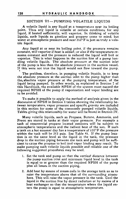
128 H Y D R A U L I C H A N D B O O K
SECTION VI - PUMPING VOLATILE LIQUIDS
A volatile liquid is any liquid at a temperature near its boiling point. Thus any liquid is volatile at certain conditions for any liquid, if heated sufficiently, will vaporize. In thinking of volatile liquids, such liquids as gasoline and propane come to mind, but water a t atmospheric pressure and near 21Z°F is just as truly a vola- tile liquid.
Any liquid a t or near its boiling point, if the pressure remains constant, will vaporize if heat is added ; or also if the temperature re- mains constant and the pressure is reduced the liquid will boil or vaporize. This is what happens in the suction line of a pump han- dling volatile liquids. The absolute pressure at the suction inlet of the pump is less than the absolute pressure in the suction vessel. If this were not true the liquid would not flow toward the pump.
The problem, therefore, in pumping volatile liquids, is to keep the absolute pressure a t the suction inlet to the pump higher than the, absolute vapor pressure at the pumping temperature, of the liquid being pumped. In other words, as explained in Section I of this Handbook, the available NPSH of the system must exceed the required NPSH of the pump if vaporization and vapor binding are to be avoided.
T o make it possible to apply the method of analysis given in the discussion of NPSH in Section I tables showing the relationship be- tween temperature, vapor pressure and specific gravity are included in this section for some of the commonly pumped volatile liquids. Tables giving this relationship for water will be found in Section IV.
Many volatile liquids, such as Propane, Butane, Ammonia, and Freon are stored in tanks a t their vapor pressure. For example a tank of commercial propane located outdoors will be subject to atmospheric temperatures and the radiant heat of the -sun. If such a tank on a hot summer day has a temperature of 1 10°F the pressure within the tank will be 213 psia. See Table 41. If the pump loca- tion is on the same level as the liquid in the tank, the pressure drop in the suction piping between the tank and pump will be suffi- cient to cause the propane to boil and vapor binding may result. T o make pumping such volatile liquids possible and reliable one of the following suggested procedures may be used.
1. Set the tank and pump so that the vertical distance between the pump suction inlet and minimum liquid level in the tank is equal to or greater than the required NPSH of the pump plus all losses in the suction piping.
2. Add heat by means of steam coils in the storage tank so as to raise the temperature above that of the surrounding atmos- here. This will raise the vapor pressure in the tank. Cool the liquid in the suction line by direct radiation or by means of a heat exchanger so that the temperature where the liquid en- ters the pump is equal to atmospheric temperature.
e
V O L A T I L E L I Q U I D S 129
3. Where heat cannot be added in the storage tank a heat ex- changer located near the pump suction capable of reducing the temperature of the liquid sufficiently below atmospheric temperature may be used.
The purpose of all three methods is to supply the pump with liquid a t a pressure above its vapor pressure at the suction inlet to the pump impeller.
REID VAPOR PRESSURE The vapor pressure of gasolines is usually obtained by the Reid
method. Because of the inadequacies of this test the true initial vapor pressure isnot obtained. The relationship between the initial vapor pressure and the Reid vapor pressure and how they vary with temperature is given in Fig. 40.
NPSH FOR PUMPS HANDLING HYDROCARBON LIQUIDS?
The NPSH requirements of centrifugal pumps are normally de- termined on the basis of handling water. I t is recognized that when pumping hydrocarbons, the NPSH to obtain satisfact,ory operation can be reduced for certain conditions. The permissible reduction in NPSH is a function of the vapor pressure and the specific gravity of the particular hydrocarbon being pumped.
It is the purpose of Fig. 37 to provide a means 'of estimating the NPSH required by a centrifugal pump when handling hydro- carbons of various gravities and vapor pressures in percentages of that required by the same pump when handling water. The cor- rection curves are based on data obtained primarily from field experience. While these data had considerable variation, they have been correlated so that the curves are considered to be usable guides. The curves have the further purpose of providing a means of comparing future experience and stimulating the accumulation of additional information.
Limitations for use of net positive suction head correction chart for hydrocarbons. Fig. 37.
1. . Use this chart for non-viscous hydrocarbons only. 2. Unusual operating conditions such as pumping hydrocarbons
close to the cracking temperature may require additional NPSH.
INSTRUCTIONS FOR USING NPSH CORRECTION CHARTS FOR HYDROCARBONS
Enter Fig. 37 at bottom with the specific gravity at pumping temperature of the particular hydrocarbon to be handled and proceed upward to the sloping line corresponding to the absolute vapor pressure in psi a t the pumping temperature. The left hand scale tCourtesy Hydrrrulic Institute. See page 6.
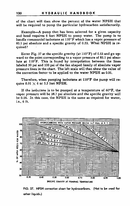
130 H Y D R A U L I C H A N D B O O K
of the chart will then show the percent of the water NPSH that will be required to pump the particular hydrocarbon satisfactorily.
Example-A pump that has been selected for a given capacity and head requires 6 feet NPSH to pump water. The pump is to handle commercial isobutane at 110°F which has a vapor pressure of 85.1 psi absolute and a specific gravity of 0.53. What NPSH is re- quired?
Enter Fig. 37 at the specific gravity (at 110°F) of 0.53 and go u p ward to the point corresponding to a vapor pressure of 85.1 psi abso- lute a t 11O0F. This is found by interpolation between the lines labeled 50 psi and 100 psi of the fan shaped family of absolute vapor pressure lines in the chart. The left scale will then show the value of the correction factor to be applied to the water NPSH as 0.91.
Therefore, when pumping isobutane at llO°F the pump will re- quire 0.91 X 6 or 5.5 feet NPSH.
If the isobutane is to be pumped at a temperature of 60°F, the vapor pressure will be 38.7 psi absolute and the specific gravity will be 0.56. In this case, the NPSH is the same as required for water, i.e., 6 f t .
SPECIFIC GRAVITY AT PUMPING W E R A T U R E
FIG. 37. NPSH correction chart for hydrocarbons. (Not to be used for
other liquids.)
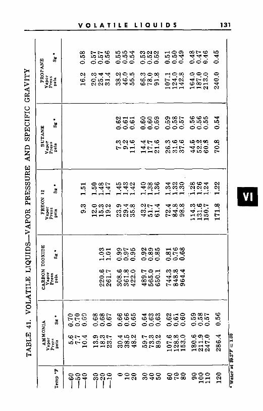
V O L A T I L E L I Q U I D S 131
00 b P - - C D m m w r l o m 0 0 b W m
0 000 000 000 000 009 0 v? v?LDv? v?v?v! v?v?" LL?v?-? "134 "1
N A r l OOQ, "I? CDwm w
000 000 000 000 0 ??e9 9?u? Lo."" ""v? v?
000 000 000 000 000 000 0 w m w mCJ7-I r ( C J m w v ) at-00 m o r ( N
l+d r( I l l I l l
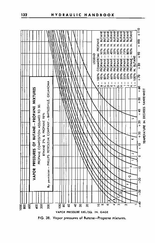
132 H Y D R A U L I C H A N D B O O K
VAPOR PRESSURE LBS./SQ. IN. G A G E
FIG. 38. Vapor pressures of Butane-Propane mixtures.
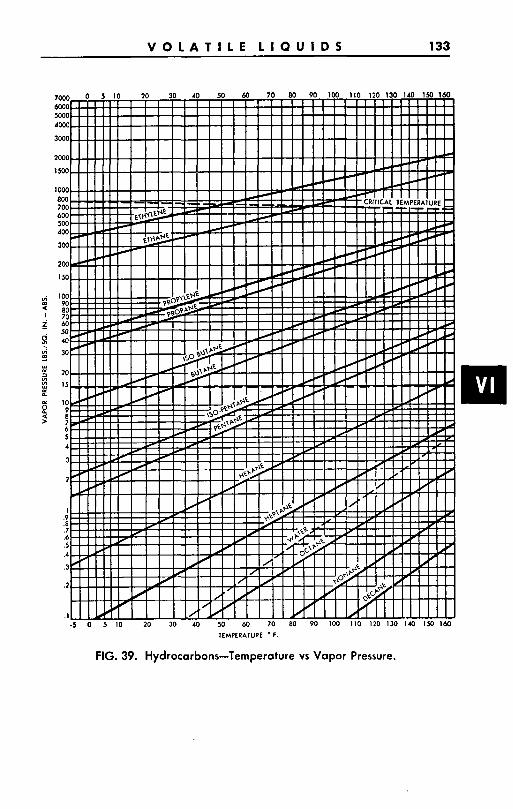
V O L A T I L E L I Q U I D S 133
TEMPERATURE ' F
FIG. 39. Hydrocarbons-Temperature vs Vapor Pressure.
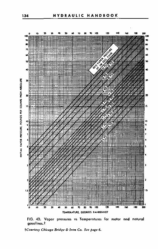
134 H Y D R A U L I C H A N D B O O K
' 0 I O 20 30 40 50 66 To 8 0 9 0 1 0 0 120 140 I60 la, m TEMPERATURE, DEGREES FAHRENHEIT
FIG. 40. Vapor pressures vs Temperatures for motor and natural gaso1ines.t
tCourtesy Chicago Bridge C Zron Co. See Page 6.
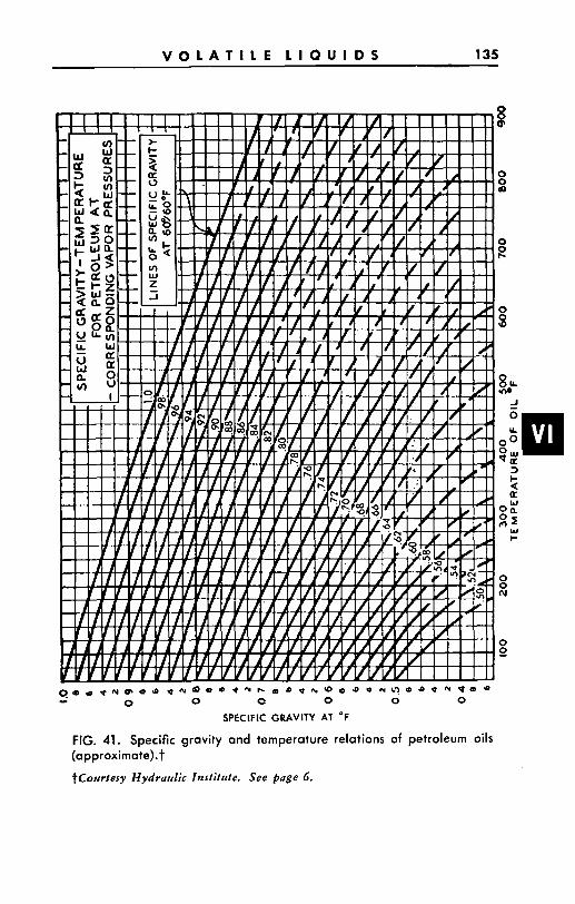
V O L A T I L E L I Q U I D S 135
Q 0 0 8
Q
0 0 (\I
0 0
SPECIFIC GRAVITY AT O F
FIG. 41. Specific gravity and temperature relations of petroleum oils (approximate) . f tCourlesy Hydraulic Institrite. See page 6.
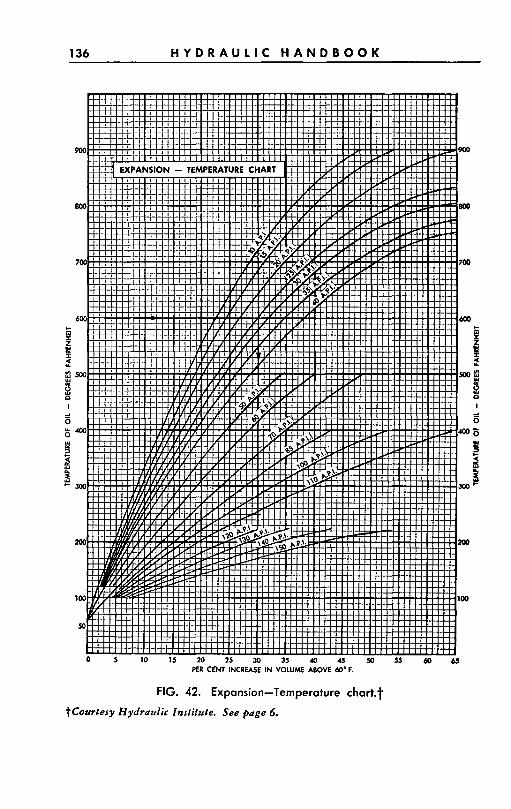
136 H Y D R A U L I C H A N D B O O K
FIG. 42. Expansion-Temperature ch0rt.f
t Courtesy Hydraulic Instilute. See page 6.
SOLIDS I N S U S P E N S I O N 137
SECTION VII-SOLIDS I N SUSPENSION
CONTENTS
Page
......... 138 Pumping Solids In Suspension - Sewage - Sand - Slurries -
............. Paper Stock - Foods - General Principles Pumping Sewage and Trash ............................................................ ,138
Pumping Sludge - Sand - Slurries .................................................... 139
Table-Fall Velocity Various Solids .............................................. 142
Chart-Friction Loss Water - Sand Mixture .............................. 142
Chart-Friction Loss - Digested Sludge ........................................ 143
Pumping Paper Stock .......................................................................... 144
Table-Required Percentage of Paper Stock to Equal Performance of Pump Lifting Kraft-Sulfa.te ...................... 145
Chart-Effect of Sulfate Paper Stock On Centrifugal Pump Characteristic .................................................................................. 145
Chart-Effect of Sulfate Paper Stock On Centrifugal Pump .......................... 146
Charts-Friction of Flow Through Pipes for Ground Wood and Sulfite Stocks .......................................................................... 147
Chart-Friction of Flow of P Fittings ..............................
Table-Weights, Volumes of Liquid Pulp Stock for Various Percentages of Air Dry Stock .................................................... 15?
Pumping Foods ............................................................. ................ 154
Illustration-Food Handling System ............................................. 156
Capacity and Efficiency ..............
138 H Y D R A U L I C H A N D B O O K
SECTION VI1 - PUMPING SOLIDS IN SUSPENSION
SEWAGE-SAND-SLURRIES-PAPER STOCK-FOODS
GENERAL PRINCIPLES
The pumping of a great variety of solid materials with liquid as the vehicle can be very successfully accomplished providing a few general principles are followed.
1. The pump should be located sufficiently below the liquid level in the suction bay so that the liquid reaches the suction eye of the impeller under a positive head.
2. All passages through the piping system, impeller, and volute should be large enough to pass the largest solid to be pumped.
3. Velocities through the pump and piping system should be such that the materials are held in suspension in the liquid. This results in less tendency to clog-less abrasion-less damage to the product pumped.
4. Velocity required in the pump varies with the pump char- acteristic and design.
5. Velocity required in the piping system depends upon the specific gravity, size, shape, consistency and friability of the material being pumped.
6. Pump materials and construction should be selected with due consideration of the substance pumped. Standard ma- terials and design are suitable for the majority of applica- tions but special metals, rubber linings, special stuffing box construction, or other features should be used in many instances.
SEWAGE AND TRASH PUMPS
The pumping of sewage is a special problem for sewage may contain a great variety of solids in suspension. I t is likely to con- tain anything that can be flushed down a toilet including towels, diapers, etc. ; anything that can fall or be thrown into a manhole; anything that can flush into a catch basin on a city street includ- ing leaves, branches, etc. ; or any type of industrial waste. . The principal consideration in pumping sewage is the passing of solids. Hydraulic performance and efficiency is secondary al- though also important. A consideration of how pumps clog will be useful in arriving at a plant design and a pump selection that will avoid this difficulty. Clogging can generally be attributed to one of the following causes:
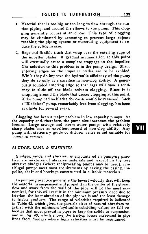
S O L I D S I N S U S P E N S I O N 139
1. Material that is too big or too long to flow through the suc- tion piping, and around the elbows to the pump. This clog- ging generally occurs a t an elbow. This type of clogging may be eliminated by screening to prevent large objects reaching the piping system or macerating equipment to re- duce the solids in size.
2. Rags and flexible trash that wrap over the entering edge of the impeller blades. A gradual accumulation at this point will eventually cause a complete stoppage in the impeller. The solution to this problem is in the pump design. Sharp entering edges on the impeller blades are to be avoided. While they do improve the hydraulic efficiency of the pump they do so only at a sacrifice in non-clog ability. A gener- ously rounded entering edge so that rags will have a tend- ency to slide off the blade reduces clogging. Since it is wrapping around the blade that causes clogging at this point, if the pump had no.blades the cause would be removed. Such a “Bladeless” pump, remarkably free from clogging, has been available for several years.
Clogging has been a major problem in low capacity pumps. As the capacity and, therefore, the pump size increases the problem lessens. Large sewage and storm water pumps with relatively sharp blades have an excellent record of non-clog ability. Any pump with stationary guide or diffusor vanes is not suitable for pumping sewage.
SLUDGE, SAND & SLURRIES
Sludges, sands, and slurries, as encountered in pumping prac- tice, are mixtures of abrasive materials and, except in the less abrasive sludges (where reciprocating pumps may be used), cen- tifugal pumps meet most requirements by having the casing, im- peller, shaft and bearings constructed in suitable materials.
In pumping practice generally the lowest velocity that will keep the material in suspension and propel it in the center of the stream flow and away from the wall of the pipe will be the most eco- nomical, for this will result in the minimum pressure drop due to friction, the least abrasion of the pipe walls and the least damage to friable products. The range of velocities required is indicated in Table 42, which gives the particle sizes of natural abrasives to- gether with the minimum hydraulic subsiding values or fall ve- locities that must prevail in pipes to keep the solids in suspension, and in Fig. 43, which shows the friction losses measured in pipe lines from dredges where high velocities must be maintained.
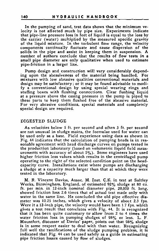
140 H Y D R A U L I C H A N D B O O K
In the pumping of sand, test data shows that the minimum ve- locity is not affected much by pipe size. Experiments indicate that pipe-line pressure loss in feet of liquid is equal to the loss by the carrier (water) multiplied by the measured specific gravity of the liquid mixture. In the turbulent flow range, the velocity components continually fluctuate and cause dispersion of ' the solids in the pipe and assist in keeping them in suspension. A number of authors conclude that the results of flow tests in a small pipe diameter are only qualitative when used to estimate pipe-friction in a larger line.
Pump design and construction will vary considerably depend- ing upon the abrasiveness of the material being handled. For mixtures with low abrasive qualities conventional materials and design may be satisfactory: or it may be found advisable to modi- fy a conventional design by using special wearing rings and stuffing boxes with flushing connections. Clear flushing liquid at a pressure above the casing pressure in the pump is piped to these parts to keep them flushed free of the abrasive material. For very abrasive conditions, special materials and completely special design are required.
DIGESTED SLUDGE
As velocities below 5 ft. per second and often 3 ft. per second are not unusual in sludge mains, the formulae used for water can be used only as a base. Field experience using data as shown in Fig. 44 indicates that the calculation of pumping heads is in rea- sonable agreement with head discharge curves on pumps tested in the production laboratory (based on volumetric liquid field meas- urements with accuracy of about 5 % ) . Some engineers have used higher friction loss values which results in the centrifugal pump operating to the right of the selected condition point on the head- capacity curve. Installations exist where pumps are discharging a sludge at a capacity much larger than that at which they were tested in the laboratory.
M. R. Vincent Daviss, Assoc. M. Inst. C.E. in test a t Saltley Works, Birmingham, England, of estimated 92% sludge at 80 cu. ft. per min. in 12-inch nominal diameter pipe, 20,000 ft . long, showed friction loss 2.6 times that of actual test made only with water in the same line. He concluded the old pipe effective dia- meter was 10.25 inches, which gives a velocity of aboct 2.3 fps. Were it a 12-inch pipe, the velocity would have been 1.7 fps. which gives a test result that correlates with Fig. 44. I t is recognized that it has been quite customary t o allow from 2 to 4 times the water friction loss in pumping sludges of 98% or less. L. F. Mountfort, discusser of Daviss' paper, points out that 98% sludge is in some respect easier to deal with than water. Recognizing full well the ramifications of the sludge pumping problem, i t is indicated that Fig. 44 can be used safely as a guide in estimating pipe friction losses caused by flow of sludges.
S O L I D S i N S U S P E N S I O N 141
SLURRIES A slurry is a liquid, usually water, in which foreign material
is suspended in varying quantities. There are many types of slur- ries such as coal, salt and the like in many different industries. The application of pumping equipment for such service depends largely on the type and quantity of foreign matter present in the mixture and the properties of the liquid carrier. No definite rules of application can be set down in this Handbook, but the following has been found essentially correct :
1.
2.
3.
4.
5.
6.
7.
8.
9.
10.
Flotation tailings from the milling of iron ores can be transported at a velocity of 5 to I fps in non-acid water. Pipe does not endure for 15 years but scouring action keeps pipe clean and reasonably free from pitting. The use of 15 year pipe-friction modifying factor appears to be too liberal and causes oversizing and overpowering. Material such as iron-pyrites ground to the fineness re- quired for flotation when thickened to a pulp can be pumped through pipes a t reasonable velocities. The head per stage should be kept as low as practical so as to hold vane-tip velocity to a minimum and to reduce ero- sion at the wearing rings. In a series of tests on a powdered glass-sand-plaster of paris mixture hardened iron impellers have proven more durable than rubber lined pumps although rubber lined pumps have their field of application. In pumping coal, the maximum quantity of fines (100 mesh) appears KO act as a lubricant in the mixture. Coal-water slurries up to 35% by weight can be pumped with a vis- cosity comparable to water at 5 fps velocity. The critical velocity for 2 to 3 inch top-size solids is 7 to 9 fps but a safe velocity is 10-12 fps in 8 inch pipe, and 11-13 fps in 10 inch pipe. Clay slurries up to 50% solids by weight can be pumped through a 4 inch pipe. SSU viscosity tests are unreliable for these slurries. The apparent viscosity varies from 25 to 85 times that for water as shown on Fig. 32.
Bentonite slurries are stiff even when they contain only 25% solids by weight. Thirty (30) percent solids by weight of some clays are too viscous to pump in a centrifugal pump. I t is possible to lift 60% solids by weight of 'iron and coke dusts or flue dirt. I t is notable that mining operations run solids as high as 70% by weight
This information indicates the great diversity of pumping ap- plications and the necessity for careful analysis of the probable field conditions before the final selection of pumping equipment.
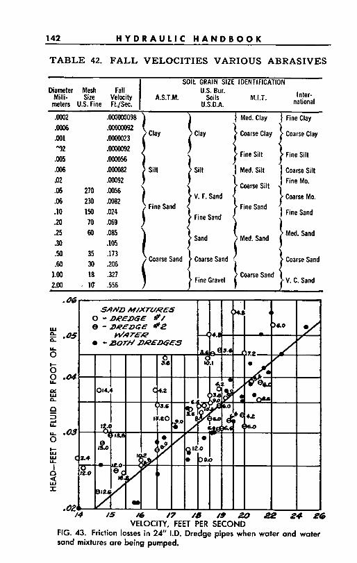
142 H Y D R A U L I C H A N D B O O K
TABLE 42. FALL VELOCITIES VARIOUS ABRASIVES
SOIL GRAIN SIZE IDENTIFICATION
lnter- national
U.S. Bur. A.S.T.M. Soils M.I.T. I U.S.D.A.
Milli- Size Velocity meters U.S. Fine Ft./Sec.
Diameter Mesh Fall
.06 270 .W56
.06 230 .ma
.10 150 .024
uwl . 10 .556
15 /6 17 18 /J 20 22 24 P6 VELOCITY, FEET PER SECOND
FIG. 43. Friction losses in 24" I.D. Dredge pipes when water and water sand mixtures are being pumped.
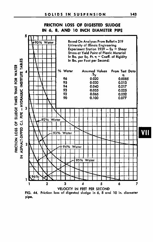
S O L I D S I N S U S P E N S I O N 143
FRICTION LOSS OF DIGESTED SLUDGE IN 6, 8, AND 10 INCH DIAMETER PIPE
Based On Analyses From Bulletin 319 University of Illinois Engineering Experiment Station 1939 - Sy = Shear Stress at Yield Point of Plastic Material In Ibs. per Sq. Ft. rl = Coeff. of Rigidity In Ibs. per Foot per Second:
1 2 3 4 5 6 7 VELOCITY IN FEET PER SECOND
FIG. 44. Friction loss of digested sludge in 6, 8 and 10 in. diameter Pipe.
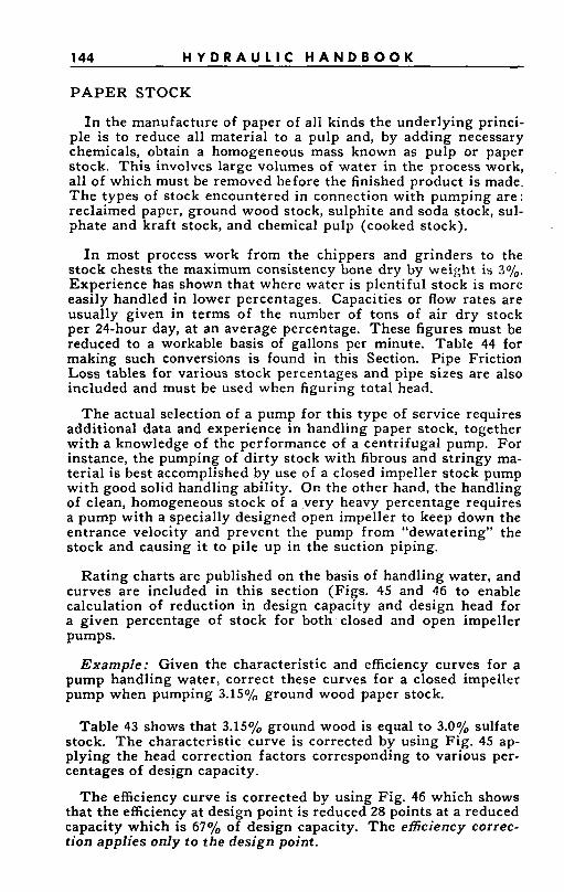
144 H Y D R A U L I C H A N D B O O K
P A P E R STOCK
I n the manufacture of paper of all kinds the underlying princi- ple is to reduce all material to a pulp and, by adding necessary chemicals, obtain a homogeneous mass known as pulp or paper stock. This involves large volumes of water in the process work, all of which must be removed before the finished product is made. The types of stock encountered in connection with pumping are: reclaimed paper, ground wood stock, sulphite and soda stock, sul- phate and kraft stock, and chemical pulp (cooked stock).
I n most process work from the chippers and grinders to the stock chests the maximum consistency bone dry by weight is 3%. Experience has shown that where water is plentiful stock is more easily handled in lower percentages. Capacities or flow rates are usually given in terms of the number of tons of air dry stock per 24-hour day, at an average percentage. These figures must be reduced to a workable basis of gallons per minute. Table 44 for making such conversions is found in this Section. Pipe Friction Loss tables for various stock percentages and pipe sizes are also included and must be used when figuring total head.
T h e actual selection of a pump for this type of service requires additional data and experience in handling paper stock, together with a knowledge of the performance of a centrifugal pump. For instance, the pumping of dirty stock with fibrous and stringy ma- terial is best accomplished by use of a closed impeller stock pump with good solid handling ability. On the other hand, the handling of clean, homogeneous stock of a very heavy percentage requires a pump with a specially designed open impeller to keep down the entrance velocity and prevent the pump from "dewatering" the stock and causing i t to pile up in the suction piping.
Rating charts are published on the basis of handling water, and curves are included in this section (Figs. 45 and 46 to enable calculation of reduction in design capacity and design head for a given percentage of stock for both.closed and open impeller pumps.
Example: Given the characteristic and efficiency curves for a pump handling water, correct these curves for a closed impeller pump when pumping 3.15% ground wood paper stock.
Table 43 shows that 3.15% ground wood is equal to 3.0% sulfate stock. The characteristic curve is corrected by using Fig. 45 ap- plying the head correction factors corresponding to various per- centages of design capacity.
The efficiency curve is corrected by using Fig. 46 which shows that the efficiency at design point is reduced 28 points at a reduced capacity which is 67% of design capacity. The efficiency correc- tion applies only t o the design point.
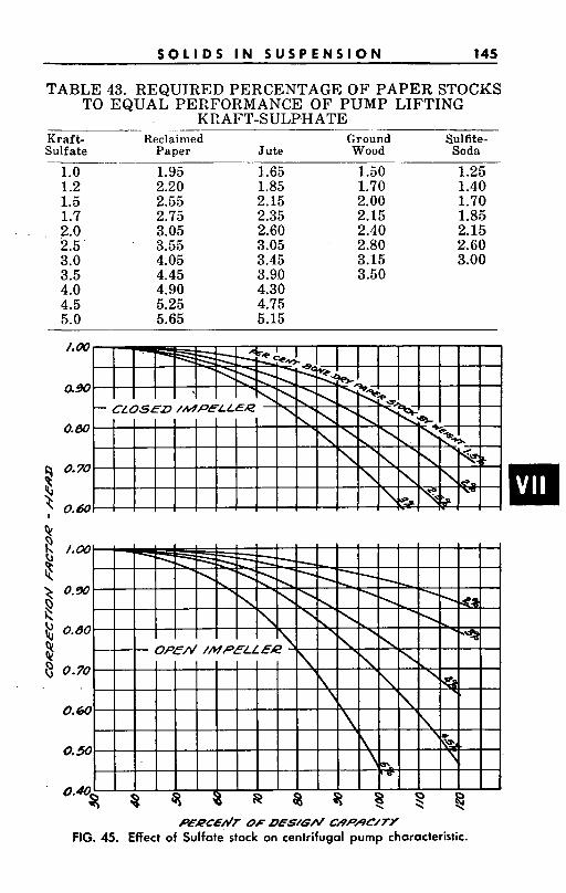
S O L I D S I N S U S P E N S I O N 145
TABLE 43. REQUIRED PERCENTAGE O F PAPER STOCKS TO EQUAL PERFORMANCE O F PUMP LIFTING
KRAFT-SULP,HATE ~ ~. .... - ___
Kraft- Reclaimed Ground Sulfite- Sulfate Paper Jute Wood Soda _______
1.0 1.2 1.5 1.7 2.0 2.5 3.0 3.5 4.0 4.5 5.0
1.95 1.65 1.50 1.25 2.20 1.85 1.70 1.40 2.65 2.15 2.00 1.70 2.75 2.35 2.15 1.85 3.05 2.60 2.40 2.15 3.55 3.05 2.80 2.60 4.05 3.45 3.15 3.00 4.45 3.9.0 3.50 4.90 4.30 5.25 4.75 5.65 5.15
a90
0.80
9 0.70
6 0.60
PEPCEdT OF DES/G/L/ CdP?c//TY FIG. 45. Effect of Sulfate stock on centrifugal pump characteristic.

146 H Y D R A U L I C H A N D B O O K
FIG. 46. Effect of Sulfate paper stock on centrifugal pump capacity and efficiency.
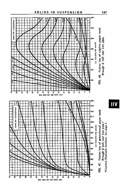
S O L I D S I N S U S P E N S I O N 147
P u.
2 U 0 c
3616 I334 001 836 SSOl I334
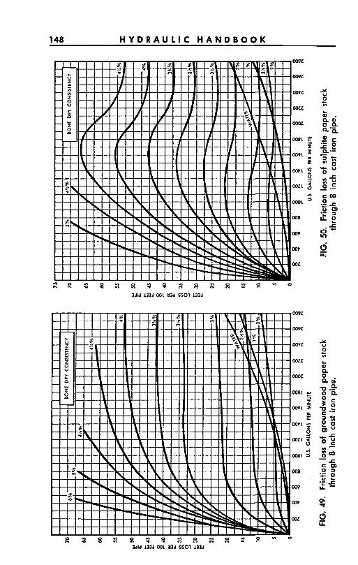
148 H Y D R A U L I C H A N D B O O K
Y
c yl
w
d E:
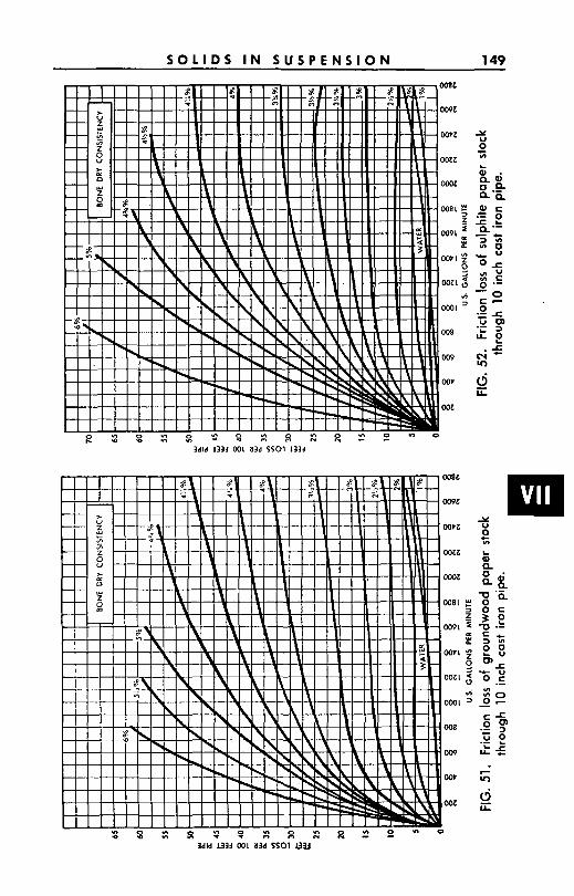
S O L I D S I N S U S P E N S I O N 149
P LL
._ - - 3dld 1331 001 13d SSOl 1334
P u.
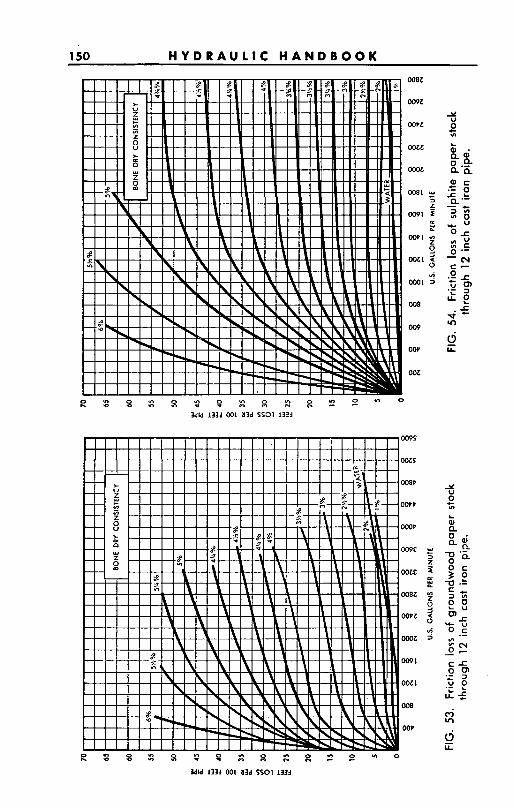
150 H Y D R A U L I C H A N D B O O K
O W L
= Y
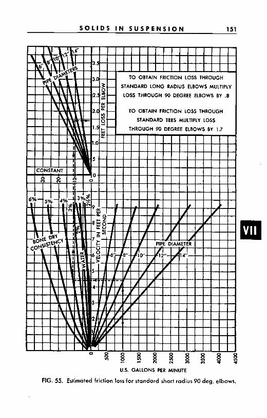
S O L I D S I N S U S P E N S I O N 151
LOSS THROUGH 90 DEGREE ELBOWS BY .8
TO OBTAIN FRICTION LOSS THROUGH
I
o a 8 a g w 8 i g $ c c N C )
U.S. GALLONS PER MINUTE
FIG. 55. Estimated friction loss for standard short radius 90 deg. elbows.
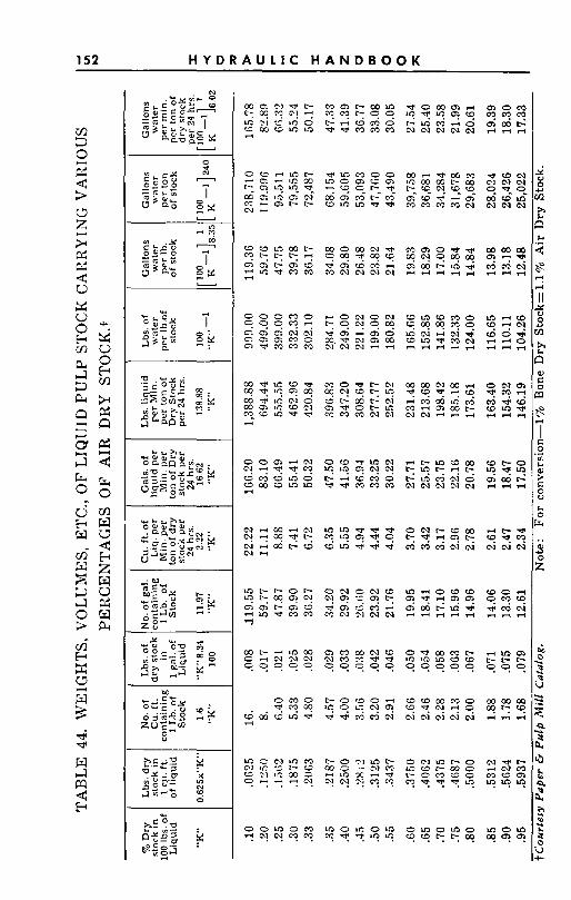
152 H Y D R A U L I C H A N D B O O K
Y
d
u Lo - c ?
u
o - m m e
99999 m m m w w
w w m m o 94"?9 " N N N
o m o m 0 ' 9 ' 9 C 1 c 1 0 9
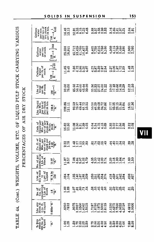
S O L I D S I N S U S P E N S I O N 153
... -
sn
154 H Y D R A U L I C H A N D B O O K
FOOD HANDLING PUMPS
Commercial canners have long desired to convey foods hy- draulically for this method represents a much less expensive means than mechanical conveyors. The problem is, of course, to handle the foods without clogging the pump or piping system and without damaging the foods. This is a manifold problem that in- volves not only the pump but also a satisfactory means of mixing the food with the liquid vehicle and finally separating the food and the liquid without damage to the product.
Hydraulic elevators that could handle such products as peas and cut beans have been on the market for many years, but new equip- ment is on the market that will handle the food so gently that the following foods have been successfully conveyed : apples, apri- cots, artichokes, cut asparagus, beans (green, lima, shelled, string, sprouts, dried or soaked), beets (peeled, diced, sugar), blueberries, brussel sprouts, carrots, cauliflower rosettes, cherries (mara- chino), chili-sauce, collard, corn (kernel), cranberries, dressings, boiled eggs, egg yolks, liquid eggs, grapes (crushed as pumped to pressing room), grits, mash, mushrooms, olives (green and ripe), onions, oranges, peas (black-eyed, field and sweet), peppers, pickles, pimientos, pineapple pulp from cores and fruit meat, white potatoes, rice (prior to soaking), soy beans (with oil ex- tracted while pumping), soups, strawberries (except Marshall ; variety), sugar (raw cane juice, cachaza, syrups, molasses), tomato catsup, tomato juice, sea foods, such as fingerlings with only 2% loss, oysters, shrimp.
Fig. 56 shows a sketch of a typical installation using pump, rod reel washer and scavenger reel with water supply tank. This in- stallation provides for vortexing of food in the hopper to the pump. This vortex is very important for i t causes very light foods that normally float on top of the liquid to sink and be drawn uni- formly into the pump suction. I t also causes long foods like string beans to enter the stream with their length parallel to the stream flow. The forced vortex is limited so air is not drawn into the Pump-
There are only six parts of a pump in contact with foods, namely; the housing or volute, back-head, removable drive shaft, packing, impeller and front-head. The interior of a pump for food han- dling service should be smoothly finished with no sharp corners, holes, pits, crevices, cracks or threads. Contact surfaces should be either ground to form a tight seal or to accommodate a rubber or single-service gasket.
Pump construction can be made to resist attack by foods, soaps, detergents and the germicidal agents used in cleaning. Stainless steel is satisfactory except for salt brines. Monel metal can be used for brines but not for corn, lima beans or peas where copper may produce darkening. Aluminum is corroded by alkalis and certain acids. Bronze is fairly corrosion resistant, but is not good
S O L I D S I N S U S P E N S I O N 155
for conveying brines in which foods are canned because of possi- ble discoloration of the end product. Experience shows that for most applications the iron fitted pump with stainless steel sleeves has been doing a creditable job. Contamination by lubricants is impossible with well designed pumps.
-
The following suggestions, based on field experience, are of- fered as a guide in pump selection and application.
1.
2.
3.
4.
5.
6.
The solids should be mixed with the liquid at a uniform rate and vortexed into the pump suction. The vortex should be limited so that air is not drawn into the pump.
Although the pump capacity required will depend upon the tonnage to be handled, the pump preferably should be se- lected so that i t will operate at its point of peak efficiency or slightly to the’r ight of this point on the characteristic curve.
The speed of the pump should be selected to meet the head requirements of the system. Heads up to l l 0 , f t . have been successful with some foods. The system should be designed to keep the head as low as possible.
The ratio of water to food solids should be as great as is practicable or economical. For peas one gallon per pound and for string beans 3 gallons per pound has been found practical.
With most foods a pump with a bladed impeller will damage the food. A pump with a “Bladeless” impeller is recom- mended.
Food solids should be carefully separated from the liquid as this is a common point of product damage.
For new uses i t is recommended that the first pumping unit be installed with a provision for variable speed operation and obser- vation of condition of the product after passing through the pump be made at the top of a riser prior to a bend. There is evidence that short radius ells, rough pipe joints or beads inside of welded pipe can cause more damage to foods than the pump itself. A velocity in the pipe of 5 fps should be tried first as this velocity appears to be above the critical for movement of food suspensions without clogging.
When pumping foods with hot water, write to the manufacturer for the required minimum suction head to obtain performance comparable with cold water. (See fundamentals concerning NPSH in Section I of this Handbook).
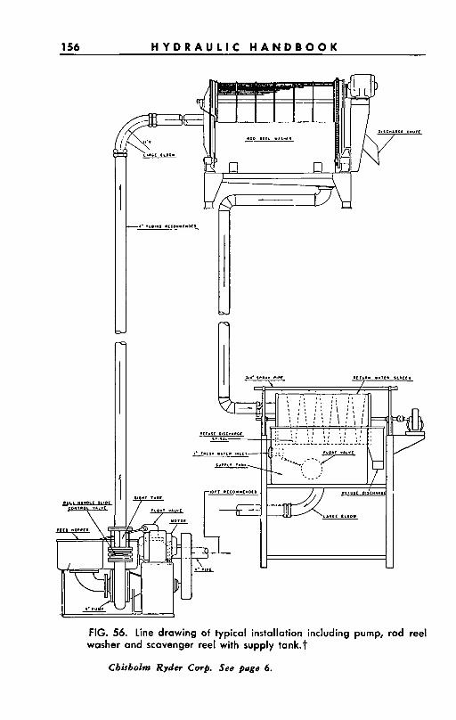
FIG. 56. line drawing of typical installation including pump, rod reel washer and scavenger reel with supply tank.t
Chisholm Ryder Cot#. See pdge 6.
C H E M I C A L L I Q U I D S 157
SECTION VIII-CHEMICAL LIQUIDS
CONTENTS
Page
Materials of Construction Used In Pumping Chemical Liquids..l58
Table-Material Selection Chart Table-Materials of Construction and
Mechanical Seals .................................................................................... 168
Packing Recommendation ...............
pH Values Various Liquids ..........
Tables-Physical Properties Calcium Chloride and Sodium Chloride ................... ............................................ 171
Table-Physical Properties Caustic Solutions .............................. 172
158 H Y D R A U L I C H A N D B O O K
SECTION VIII-CHEMICAL LIQUIDS I
MATERIALS O F CONSTRUCTION FOR PUMPING VARIOUS LIQUIDSt
Although pumps produced by various manufacturers will differ in design and performance detail, they follow the same general pattern in the utilization of materials for handling specific liquids. This is natural since the manufacturer has little control over the corrosive reaction between the materials and the liquids handled and, hence, must use those types which experience has indicated as being most satisfactory for the particular application under consideration.
Because of the many variables which influence the rate at which corrosion may occur, it is not possible to make positive predictions which will cover every application. However, for the guidance of both pump manufacturers and users, the Materials Specifications Committee of the Hydraulic Institute has compiled a list of the liquids more commonly encountered in industry, along with the materials generally associated with their use. This data is shown in Table 46.
DATA ON VARIOUS LIQUIDS The liquids are assumed to be of commercial quality and of the
degree of purity usually encountered. However, one must recog- nize that the presence of a foreign substance, even in small per- centages, may, and frequently does, have a profound effect upon the corrosiveness of the solution and, hence, upon the choice of materials. For instance, the presence of a small percentage of so!uble chloride or other halide in many of the liquids included in the table may greatly intensify their corrosive properties. Con- versely, certain substances, such as the chromates and dichromates, may inhibit the corrosive action of many solutions on ferrous metals. Further, some liquids, noticeably the vegetable oils, while relatively inactive when fresh, may, upon exposure to heat and/or the atmosphere, turn rancid and become quite corrosive. While cast iron might be used safely with such oils when sweet, it would not necessarily be satisfactory after they had soured. I n the latter case, other, more resistant materials would probably be required.
In some cases the satisfactory use of a particular material is restricted to a definite temperature and/or concentration range, and where this is known to occur, the limitations are so noted in the tabulation. As the corrosion rate usually increases with tem- tAbridged from Standards of Hydraulic Institute. See page 6.
C H E M I C A L L I Q U I D S 159
perature, the latter becomes an important factor in making a material selection. Where the space is left blank in the appropriate column, it is assumed the materials listed are suitable over the ranges of concentration and temperature normally encountered.
PUMP CONSTRUCTION MATERIALS The materials listed are those most commonly used in the
principal parts of the pump, such as casings, impellers, cylinders, and, hence, are primarily castings. Wrought materials, such as shafts, should, where practical, be of similar composition to the castings used, and, in the case of ferrous materials, would carry the designation of the American Iron and Steel Institute. Cross- reference is made to such materials in the listings.
Since it is not possible in any generalization to say with cer- tainty that any one material will best withstand the corrosive attack of a given liquid, more than one type is usually included. However, the order of listing does not necessarily indicate relative superiority, as certain factors predominating in one instance may be sufficiently overshadowed in others to' reverse the arrangement.
When the liquid to be handled is an electrolyte, combinations of dissimilar metals which may promote galvanic reactions should, where practical, be avoided. The rate of corrosion, where metals widely separated in the galvanic series are used, will depend upon such things as the nature of the electrolyte, temperature, velocity, and particularly, the relative cathode-anode surface area. Although bronze fittings in an iron pump handling sea water may initially accelerate the corrosion of the surface of the iron, the overall rate is sometimes sufficiently low to make the use of large pumps, so fitted, economically sound.
SELECTION O F MATERIALS The pump construction and materials selected as suitable for
each application are tabulated opposite the corresponding liquids in Table 46. To simplify identification, each construction and ma- terials selection is designated by descriptive letters or a number as follows:
(1) Iron or Bronze Fitted .... SF (3) All Bronze .................... AB (2) All Iron ............................ AI (4) Types 8, 9, 10, 11 ............ SS To simplify recording, the symbol SS is used in those cases
where types 8, 9, 10, 11 would normally be listed. This does not necessarily mean, however, that all are equally effective in all environments. It merely means that each type has been satisfac- torily applied in handling that liquid under some, possibly all, conditions.
Other materials, including corrosion resisting steels, are listed by number in accordance with Table 45.
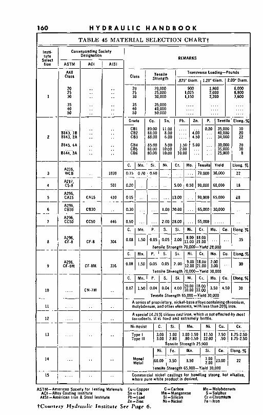
160 H Y D R A U L I C H A N D B O O K
.... I . . .
. . . . 4.00
. . . . 4.50
1.50 5.00 2.00
10.00
TABLE 45 MATERIAL SELECTION CHARTt
- . --__.- 0.20 35,000 IO . . . 40,000 20 . . . 34,000 22
_ _ . 30,000 20 . . . . . . 35.000 10 . . . . . . 25.000 8
-- - Insti- tute
Select tion
CB4 CB5 CB6
Corresponding Society Desianation
85.00 88.00 80.00
REMARKS - ASTM
A48 Class
20 25 30
35 40 50
- _ _ ACI -
Transverse Loading- Pounds
1,800 6,000 2.000 6.800
1,150 2.200 7,600
I Tensile Class ) Strength
20,000 25.000
30 30.000 1
35.000 :i I 40,000 50 50,000
.... .... .... . . . . I . . . . I .... .... .... ..,. -_ Grade I Cu.
__ Sn.
11.00 8.00 6.00
5.00 10.00 10.00
__ Pb. I Zn. I P. 1 Tensile I Elonn.'
6143; .I B 6143, 2A
B145. 4A
81441'3A
.. .. ..
2
A216. WCB
A217. c5-8
A296. CAI5
__
--
Mo. 1 Tensile Yield Elong. 7
. . . 1 70.000 36.000 22 - - ~ _ _
0.50 190.000 60,000 18 ~ _ _ ~ _ _ _
. . j 90.000 65.000
3 ~
4
1030 ~
501
1.35 I 0.70 1 0.60 -- - .- . . . . . . -__-
1.15 . . . . . .
1.30
1.50
--- 1CO8 1 ::o I
-_ . . . 5.00
. . . 13.00
-- 5
6
I-
CAI5 410
A296. CB30
A296. CC50
--
__
A296 CF-8'
A296. CF-8M
.~
....
CB30 . . . ..
. . . 55,000 CC50 446
---_.--- Si. 1 Ni. 1 Cr. I Mol 1 Cu; [€long.:
ile Strength 70.000-Yield 28.000 S. I Si. I Ni. I Cr. I Mo. I Cu. 1 Elong.:
S. I o.05 oo 8.00 18.00 35 j ' 11.00 21.00, CF-8 304
-I -I-I-I-I-I-
316 CF-8M
CN-7M LO7 1.50 1 0.04 t , I ,
e Str;ngth 65.000-Yield 30,000 Ten A series of proprietary. nickel base alloys containingchromium. molybdenum, and other elements. with less than 20% iron.
A special 14.25% silicon cast iron, which is not effected by most corrodents. I t is hard and extremely brittle.
Ni-Resist I C. I Si. I Mn. 1 Ni. I Cu. I Cr.
Type I 3.00 1.00 1.00-1.50 17.50 7.50 1.75-2.5( Type II 3.00 2.80 30-1.50 22.00 1 .50 I 1.75-2.5(
Tensile Strength 25,000 I Ni. I Fe. I Mn. I Si. I Cu. I Elon&%
- -~ -~ _ _ - _ _ ~ ~ _ _ ~ -
13 ....
I-I-I-1-1-1- 14
__ 15
z:i 160.00 I 3.50 1 3.50 I ;:!: 123.00 I 22
Tensile Strength 65,000-Yield 30,000 - - ~ ~
Commercial nickel castings lor ,handling strong. hot alkalies. where pure white product is desired.
....
- ....
.. -
ASTM-American Society for Testing Materials Cu =Copper C=Carbon Mo = Molybaenum ACI- Alloy Casting Institute Sn =Tin Mn=Manganese S=Sulphur
AIS-American Iron 8 Steel Institute Pb =Lead Si=Silicon Cr =Chromium Zn-Zinc Ni=Nickel Fe=lron
?Courtesy Hydruialic Institute See Puge 6.
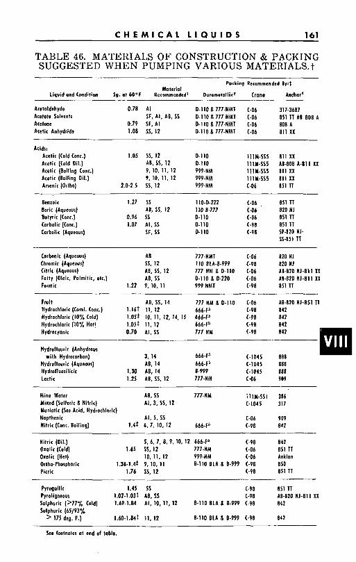
C H E M I C A L L I Q U I D S 161
TABLE 46. MATERIALS O F CONSTRUCTION & PACKING SUGGESTED WHEN PUMPING VARIOUS MATER1ALS.t
Pocking Recommended By:$ Materiot
l iquid ond Condition Sg. 01 60°F Recommended' burm"o l l i r2 Crane Anchor' -
Acetaldehyde 0.78 A I 0-110 8 177-NMT (-06 311-3687 Acetate Solvents Acetone 0.79 SF, A I 0-110 8 771-NMT (-06 808 A
SF, AI , AB. 55 0-110 8 777-NMT (-06 851 I T AB 808 A
Acetic Anhydride 1.08 ss, 12 D-110 8 777-NMT (-06 811 xx
Arids: Acetic (Cold Conc.) 1.0s 5s. 12 0-110 I l lM-IS5 811 XX Acetic (Cold Dil.) AB, 55, 12 0-110 111M-SSZ AB-808 A411 XX Acetic (Boiling Conc.) 9, IO, 11, 12 999-NM 11IM-SS5 E l l XX Acetic (Boiling Oil.) 9, IO. 11, 12 999-NM IIIM-SSS 811 XX Arsenic (Ortho) 2.0-2.5 5s. 12 999-NM (-06 851 TT
Benzoir 1.27 55 110-D-222 (-06 , 851 n
Carbolic (Conc.) 1.07 AI, 55 0-110 (-98 851 n Boric (Aqueous) AB, 55, I? 110-8-777 C-06 820 NJ Butyric (Conc.) 0.96 55 D-110 (-06 851 IT
Carbolic (Aqueous) SF, 55 0.110 (-98 5)-820 NJ- SI-851 n
Carbonic (Aqueous) AB 777-NMT (-06 820 NJ Chromic (Aqueous) $5, 12 110 BLA-8-999 (-98 820 NJ Citrir (Aqueous) AB, 55. 12 777 NM B D-110 (-06 AB-820 NJ-811 XX Folly [Oleic, Palmitic, etc.) AB, SS D-110 8 D-220 (-06 A8420 NJ-811 XX Formic 1.22 9, IO, 11 999 NMT (-98 851 TT
Fruit AB. 5 5 , 14 777 NM 8 0-110 (-06 . 18-820 NJ-851 T l Hydrochloric (Coml. Conc.) 1.16$ 11, 12 666-F5 (-98 842 Hydrochloric [IO% Cold) 1.05$ IO, 11, 12, 14, 15 666-F5 (-98 842 Hydrochloric (10% Hot! 1.05t 11,12 666-F5 (-98 812 Hydrocyonic 0.70 AI, 55 777 NM (-98 842 __ Hydroflouric (Anhydrous
with Hydrocarbon) 3, 14 666-F5 (-1045 888 Hydroflouric (Aqueous) AB, 14 666-F5 (-1045 888 Hydrofluosilicic 1.30 AB, 14 0-999 (-1045 888 Lactic 1.21 AB, 55, 12 777-NM (-06 909
Mine Water AB, 55 777-NM il lM-SS1 386
Muriatic (See Acid, Hydrochloric) Napthenit A I , I, 55 (-06 909 Nitric (Conc. Boiling) 1.4t 6, 7, IO, 12 666-F5 (-98 842
Mixed (Sulfuric 8 Nitric) AI, 3, 55, 12 (-1045 317
Nitric (Dil.) 5. 6. 7, 8. 9, IO. 12 666-F5 Oxalic (Cold) 1.65 55, 12 777-NM Oxalic (Hot) IO, 11.12 999-NM Ortho-Phosphoric 1.36-1.4t 9, IO, 11 8-110 BLA 8 8-999 Picric 1.76 SS. 12
Pyrogallic 1.45 SS Pyroligneous 1.02-1.03t AB, 55 Sulphuric (>77% Cold) 1.69-1.84 AI, IO, 11, 12 8-110 BLA 8 8-999 Sulphurir (65/93%
-
> 175 deg. F.) 1.60-1.84i 11, 12 8-110 BLA 8 8-999
See footnotes at end of table.
(-98 842 (-06 851 TT (-06 Anklon (-98 850 (-98 851 TT
(-98 851 TT (-98 18-820 NJ-811 XX (-98 842
(-98 842
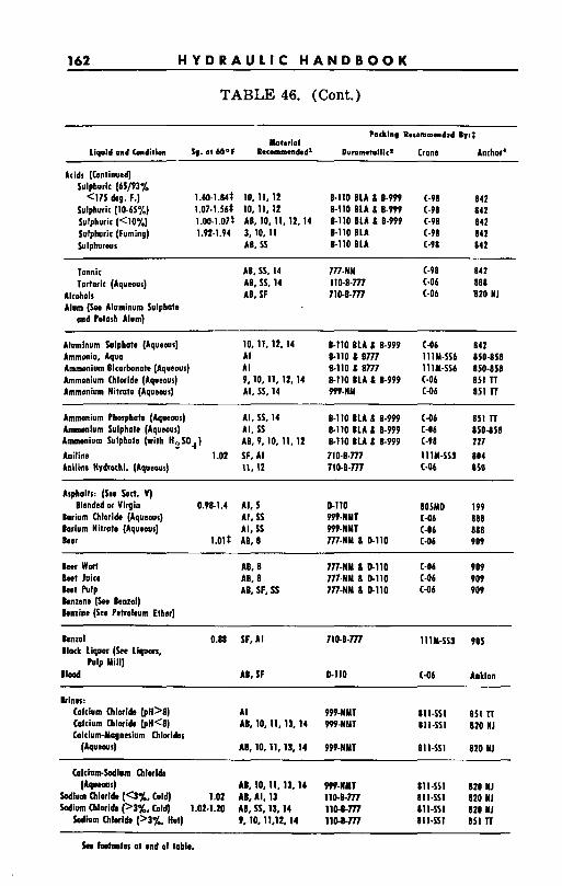
162 H Y D R A U L I C H A N D B O O K
TABLE 46. (Cont.)
Packinn hrommendrd If:$ Moterial
liquid and Condition Sg. at WOF R*commenbdl Dumnntallic* Crane Anchor
Acids (Continued) Sulphuric (65/93%
<l75 deg. F.) 1.60-1.84t 10, 11,12 8-110 BLA I B-939 (-98 842 Sulphuric ( 1 0 4 % ) 1.07-1.56$ 10, 11, 12 8-110 BLA I 8-999 (-98 842 Sulphuric (<lo%) 1.00-1.07t AB, 10, 11, 12, 14 8-110 811 I 8-999 (-98 842 Sulphuric (Fuming) 1.92-1.94 3, 10, 11 8-110 BLA (-98 841 Sulphurous AB, SS 8-110 BLA (-98 842
~~
Tannic AB, 55, 14 777-NM (-98 a42 Tartaric (AqueoUs) AB, 55. 14 i i o - ~ - n 7 (-06 888
Alcohols AB, SF 710-8-777 (-06 820 NJ Alum (See Aluminum Sulphate
and Potash Alum) ~~~ ~ ~
Aluminum Sulphate (Aqueous) 10, 11, 12, 14 8-110 BLA I 8-999 (-06 842
Ammonium Chloride (Aqueous) 9,10, 11, 12, 14 8-110 BLA I E999 (-06 8Sl n Ammonium Nitrate (Aqueous) AI, SS, 14 999-NM (-06 851 TT
Ammonium Phosphate (Aqueous) AI, 55, 14 8-110 8LA I 8-999 (-06 851 n Ammonium Sulphate (Aqueous) AI, SS 8-110 BLA I 8-999 (-06 850-8S8 Ammonium Sulphate (with H2S04) AB, 9, 10, 11, 12 8110 BLA I 8-999 (-98 211
Aniline llydrothl. (Aqueous) 1 1 , l l 710-8-777 (-06 I S 0
Ammonia, Aqua A I 8-110 I e777 l l lM- IS6 850-858 Ammonium Bicarbonate (Aqueous) A I E110 I 8777 lllM-SS6 850-858
Aniline 1.02 SF, A I 7 1 o - ~ - n 7 111P-113 804
Asphalts: (See Sect. V) Blended or Virgin 0.981.4 AI, I D-110 80SMD 199
lorium Chloride (Aqueous) AI, SS W9-NMT (-06 888 Iar ium Nitrate (Aqueous) AI, IS W9-NMT (-06 888 Beer 1.01$ AB, 8 n 7 - n ~ I D-110 (-06 909
I n r Wort AB, 8 777-NM I D-110 (-06 909 loot Juice AB, 8 777-NP I D-110 (-06 909 k t Pulp AB, SF, SS 777-NP I D-110 (-06 909 Bmzene ( k e Benzol) knz ine (be Petroleum Ether]
Benzol 0.88 I lack Liquor (be Liquors.
IloDd
k insr :
Pulp Mill)
Calcium Chloride (pH>8) Calcium Chloride (pW8) Calcium-Magnesium Chlaidss
( h u e d
Calcium-Sodium Chloride (bms)
b d i r m Chlorlde (<3%, Cold) 1.02 bdim Chloride (>3%, bid) 1.02-1.m
Sodium Chloride (>3%, Hot)
SF, A I 710-8-777 1 111-153
AB, SF D-110 (-06
A I 999-NMT 811-111 AB, 10, 11, 13, 14 999-NMT 811-SSl
AB, io, i i , i ~ , i 4 ~W-NAIT 811-111
905
A n k h
as1 TT 820 WJ
820 NJ
AB, io, 11.13.14 Ppp-wni 81 1 -SSl AB, AI, 13 110-8777 811-111 AB, SS, 13, 14 110-E-777 811-111 9, 10. 11.12. 14 1lM-777 811-151
820 111 620 111 820 111 €41 TI
h fDotnohr at end of table.
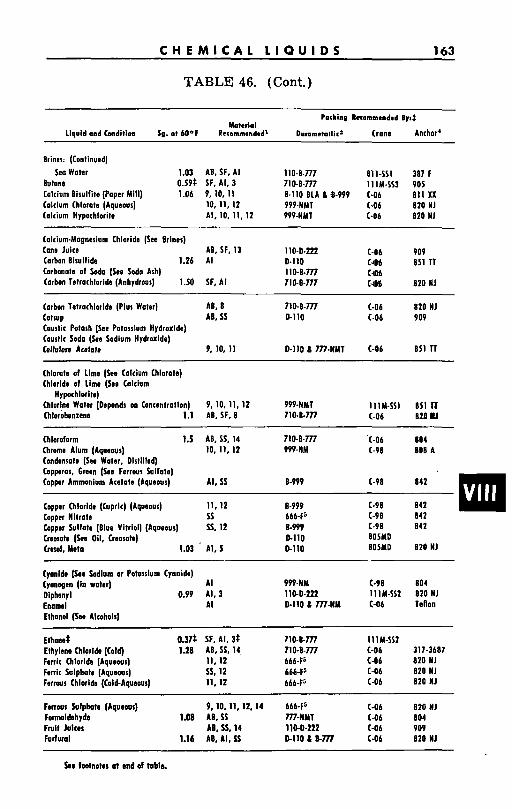
C H E M I C A L L I Q U I D S 163
TABLE 46. (Cont.)
Pocking Recommended Byit k t e r i o l
l iqu id and Cmditioa Sg. o? 60°F Recommended' Durometollic' Crane Anchor'
Brines: (Continued)
Sea Waler 1.03 AB, SF, A I 110-8-777 811-111 387 F Butane 0.59s SF, AI, 3 710-8-777 111M-IS3 905 Calcium Bisulfite (Paper Mill) 1.06 9 , 10, 11 8-110 BLA I % - 9 9 9 (-06 811 xx Calcium Chlorate (Aqueous) 10, 11,12 999." (-06 820 N J Calcium Hypochlorite AI, 10, 11, 12 999-NMT (-06 820 N J
Calcium-Magnesium Chloride (See Brines) Cane Juice AB, SF. 13 110-0.222 (-06 909 Carbon Bisulfide 1.26 A I 0-110 cJm 851 n Carbonote of Sodo [See Sodo Ash) 110-8-777 CJM Corbon Tetrachloride (Anhydrous) 1.50 SF, A I 710-8-777 c4m 820 NJ
Carbon Tetrachloride (Plus Water) AB, 8 110-8-777 (-06 820 NJ Catsup AB, 55 D-110 (-06 909 Caustic Potash (See Potassium Hydroxide) Caustic Soda (See Sodium Hydroxide) Cellulose lcotate 9, 10, 11 D-IIO a ~ - N M T (-06 851 n ~~
Chlorate of Lime (See Calcium Chlorate) Chloride of Lime (See Calcium
Hypochlorite) Chlorine Water (Depends on Contentrollon) 9 , 10, 11, 12 999-NMT 111M-SS1 851 IT Chlorobenzene 1.1 AB, SF, 8 710-8-777 GO6 828 U
Chloroform 1.5 AB, 55, 14 710-8-777 (-06 804 Chrome Alum (Aqueous) 10, 11,12 999-NM ( -98 808 A Candonsate (See Water, Dlstilled) Copperas, 6rean (See Ferrous Sulfate)
842 illll Copper Ammonium Acetate (Aqueous) AI, SS 8-999 ( -98
Capper Chlorlde (bpr lc) (Aqueous) 11,12 8-999 ( -98 Coaaar Nitrate 5s 666-F5 ( -98 842 &;;or Sulfate (Blue Vitriol) (Aquews) Creosote (See Oil, Creosote) (raol, Yeto 1.03 11, 5
Cyanide [See Sodlom or Potasslum Cyanide) Cyanogen (in water) A I Diphenyl 0.99 AI, 3 Enamel A I Elhanal (he Alcohols)
55, 12 8-999 ( -98 CllO 8OSMO DllO 805MO
999-NM ( -98 110-0-222 1 I 1 M-SS2 D-110 8 7 7 7 - N M (-06
842
820 NJ
804 820 NJ Teflon
E 1 h a n e 0.37$ SF, AI, 3t Ethylene Chloride (Cold) 1.28 AB, SS, 14. Ferric Chloride (Aqueous) 11,12 Ferric Sulphate (Aqueous) SJ, 12 Ferrous Chloride (ColbAquwrrs) 11,12
710-8-777 1 1 I M-IS? 710-E-777 (-06 666-f6 (-06 666-Fs (-06 6664' (-06
317-3681 820 NJ 820 NJ 820 NJ
Ferrous blphata (Aqoews) 9, 10, 11, 12, 14 666-F5 (-06 820 NJ Formaldehyde 1.08 AB,SS 777-NMT (-06 804 Fruit Joicer AB, SS, 14 110-D-222 (-06 909 Forfuml 1.16 AB, AI, 55 DllO 6 E777 (-06 820 NJ
Or foolnates at end of t ab la
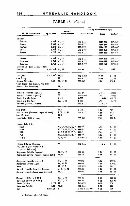
164 H Y D R A U L I C H A N D B O O K
TABLE 46. (Cont.)
Pocking Recommended By:$ Materim1
Liquid and Condition Sg. ot 60°F Retommmded' Duromefallicz Crone Anchor'
Gosolines: Pentane 0.63t AI, SF 710-8-777 11 11-513 317-3687
Heptane 0.69t AI, SF 710-8-777 ll lM-SS3 317-3687 Oclone 0.71# AI, SF 710-6-777 1 llM-SS3 317-3687 Nonane 0.72# AI , SF 710-6-777 11 IM-SS3 317-3687
Oecone 0.73# AI , SF 710-8-777 l l lM- IS3 317-3687 Undecone 0.74t AI , SF 710-6-777 lllM-SS3 317-3687 Dodetane 0.75: AI, SF 710-8-777 111M-SS3 317-3687
Hexane 0.66t AI, SF 710-6-777 l l lM-113 317-3681
Gtaubers Salt [See Sodium Sulfate) Glucose 1.35-1.44t AB, SF 777-NM (-06 1108 __ -~
t l u s (Hot) 1.20.1.25t SF, AI 110-0-222 81OW 317 W Glue Sizing AB 110-0-222 81OW 317 W Glycerol (Glycerin) 1.26 AB, SF, A I 777-NMT (-06 820 NJ Green liquor (See liquors, Pulp Mill) Heptane (See Gosolines) SF, AI
Hydrogen Peroxide (Aqueous) 5s 666-F5 (-104s 820 NJ Hydrogen Sulfide (Aqueous) 5s 110-0-222 (-98 820 NJ Kaolin Slip [In Water) AI, 3 6-777 111M-SS1 851 n Kerosene (See Oil, Kerosene) 710-6-777 11 1M-SS3 Kaolin Slip (In Acid) 10, 11, 12 6-999 (-98 851 n
lord (Hot) SF, A I 0-110 (-06 909 Lend Acetate (Aqueous) (Sugar of lead) 9, 10, 11. 14 110-0-222 (-98 842
Lime Water (Milk of Lime) A I 777-NlilT SS6J 820 HJ Lend (Molten) AI, 3 (-98 841
liquors, Pulp Mill: Black Green White Pink Sulfite
A1,3,9,10,11,12,14 666-F5 (-06 811 xx A1,3.9,10,11,12,14 666-F5 (-06 811 xx AI.3.9,lO. 11,12,14 666-F5 (-06 811 xx AI , 3,9,10,11,12,14 666-F5 (-06 811 xx 9,10, 11 8-110-BLA (-06 811 xx
~ ___
lithium Chloride (Aqueous) A I 110-6-777 lIlM.-SSl 811 XX lye, Coustic (See Potassium 8
Sodium Hydroxide) Mognesium Chloride (Aqueous) 10. 11, 12 999-NM (-06 851 n Magnesium Sulfate [Aqueous) (Epsom Salts) AI , SS 999-NM (-06 851 TT
__ ~ __ Monganese Chloride (Aqueous) AI, 55.12 999-NM (-06 820 NJ Manganous Sulfote (Aqueous) AB, AI , SS 999-NM (-06 820 NJ Mosh AB, SF, 8 110-0-222 (-06 909 Mercuric Chloride (Very dil. Aqueous) 9, 10, 11, 12 999-ttM (-06 851 TT Mercuric Chloride (Coml. Conc. Aqueous) 11, 12 999-NM (-06 851 TT
_ _ ~ . - Mercuric Sulfate (in HISO&) 10,11,12 999-NM ( -98 820 NJ Mercurous Sulfate (in HISO&) 10. 11, 12 999-NM (-98 820 NJ Methyl Chloride 0.92t AI 710-8-777 (-06 856 Methylene Chloride 1.34 AI, 8 710-6-777 (-06 856 Milk 1.03-1.04 B D-110 or 777-NM (-06 909
_. ~- See footnotes at end of table.
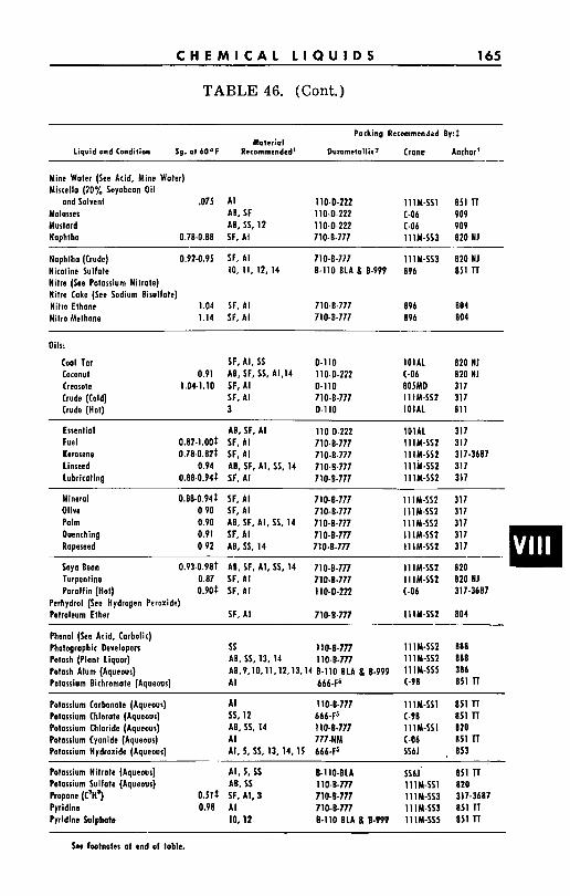
C H E M I C A L L I Q U I D S 165
TABLE 46. (Cont.)
Parking RetommrnJed Ry:t Material
l iquid ond Condition Sg. a1 60°F Recommended' Duromrtallica Crane Anchor4
Mine Woter (See Acid, Mine Woter) Mistella (20% Soyabean O i l
Molasses AB, SF 110-D-222 (-06 909 Mustard AB, 55.12 110-D-222 (-06 909
and Solvent .075 A I 110-D-222 111M-SS1 851 T I
Naphtha 0.78-0.88 SF, AI 710-8-777 lllM-SS3 820 NJ
Naphtha (Crude) 0.92-0.9S SF, AI 710-8.777 111M-SSJ 820 NJ Nicotine Sulfate 10, 11, 12, 14 8-110 BLA B 8-999 896 B S l n Nitre (See Potassium Nitrate) Nitre Coke (See Sodium Bisulfate) Nitro Ethane 1.04 SF, AI 710-8-777 896 804 Nitro Methane 1.14 SF, AI 710-8-777 896 804
Oils:
Coal Tar Coconut Creosote Crude (Cold) Crude (Hot)
Essential Fuel Kerosene Linseed Lubricating
SF, AI, SS D-110 0.91 AB, SF, 55. A1,14 110-0.222
1.04-1.10 SF, AI D-110 SF, AI 710-8-777 3 D-110
AB, SF, A I 110-0-222 0.82-1.00t SF, AI 710-8-777 0.78-0.82t SF, AI 710-8-777
0.94 AB. SF, A I , 55. 14 710-8-777 0.88.0.94t SF, A I 710-8-777
l O l A L (-06 8OSMD 11 1M-SS2 101AL
820 NJ 820 NJ 317 317 81 1
101111 11 1M-SS2 11 lUSS2 11 1M-SS2 11 1M-SS2
317 317
31 7 317
317-3687
Mineral 0.88-0.94t SF, AI 710-8-777 111M-SS2 317 Olive 0 9 0 SF, AI 7104-777 111M-SS2 317 Palm Quenching - 0.90 AB, SF. A I , 55, 14 710-8-777 111M-SS2 317
0.91 SF, AI 710-8-777 IlIM-SSP 317 Rapeseed- 0.92 AB, 55, 14 710-8-777 111M-SS2
3l7--- Soya Bean 0.93-0.98t AB, SF, AI , SS, 14 710.8-777 111M-SS2 820 Turpentine 0.87 SF, A I 7104-777 111M-SS2 820 NJ Paraffin (Hot) 0.90t SF, A I 110-D-222 (-06 317-3687
Perhydrol (See Hydrogen Peroxide) Petroleum Ether SF, A I 710-8-777 111M-IS2 804
Phenol (See Acid, Carbolic) Photographic Developers ss 110-8-777 ll lM-IS2 888 Potash (Plant Liquor) AB, 55, 13, 14 1 io-8-7n IllM-SS2 888 Potash Alum (Aqueous) A8,9,10,11,12,13,14 8.110 BLA 8 8.999 111M-SSS 386 Potassium Bichromate (Aqueous) A I 666-F5 ( -98 8Sl TT
Potassium Carbonote (Aqueous) A I 110-8-777 111M-SS1 851 TI
Potassium Chloride (Aqueous) AB. 55. 14 1104-777 111M-SSI 820 Potassium Chlorate (Aqueous) ss, 12 666-F5 ( -98 811 n
Potassium Cyanide (Aqueous) A I 777-NM (-06 I 5 1 n Potassium Hydroxide (Aqueous) AI , 5, 55, 13, 14, I S 666-F5 1161 853
Potassium Nitrote (Aqueous) A I , 5, SS B-110-BLA SS6J. 8S1 n Potassium Sulfate (Aqueous) AB, SS 110-8-777 111Y-SS1 820 Propane (C'H') 0.5lt SF, AI , 3 710-8-777 lllM-113 317-3687 Pvridins 0.98 A I 710-8-777 111M-SS3 851 T I Pyridlne Sulphale 10,12 8-110 BLA 8 8-999 ll lM-SI5 851 n
See loatnotes ot end of table.
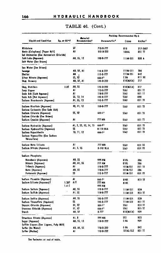
166 H Y D R A U L I C H A N D B O O K
TABLE 46. (Cont.)
Pocking Recommendad By*$ &io1
Llquid and Condition Sg. 01 bO°F Recommended' Dummetollic' Crane Anchor'
Phidoleno SF 710-8-777 810 317-3687 Rosin (Colophony) (Paper Mill) AI 110-0-222 1OOAL 8S1 TT Sa1 Ammoniac (See Ammonium Chloride)
Salt Water fSee Brines1 Salt Lake (Aqueous) AB, 55, 12 110-8-777 l l lM-SI1 808 A
Sea Water (See Brines) Sewage Shellac Silver Nitrate (Aqueous) Slop, Brewery
AB, SF, AI 110-8-777 111M-I l l 386 AB . 110-8-777 111M-IS1 842 IS, 12 666-F' (-06 811 xx AB, SF, AI 110.0-222 810(MICA) 317
Slop, Distillers 1.0s AB. SS 110-0-222 8lO(MICA) 317 Soap Liquor A I 110-8-777 5161 (51 I T Soda Ash (Cold Aquews) AI 110-8-771 1161 1151 I T Soda Ash (Hot Aqueous) 55, 13, 14 110-8.777 1161 888 Sodium Bicnrbonole (Aqueous) AI, 55, 13 110-8-777 1161 851 TT
Sodium Bisulfote (Aqueous) Sodium Carbonote (See Soda Ash) Sodium Chlorote (Aqueous) Sodium Chloride (See Brines) Sodium Cyanide (Aqueous)
Sodium Hydroxide (Aqueous) Sodium Hydrosulfite (Aqueous) Sodium Hypochlorite Sodium Hyposulfite (See Sodium
Thiosulfote)
Sodium Meln Silicote Sodium Nitrate (Aqueous)
10, 11. 12 110-8-777
IS, 12 6664'
AI 777-NM
AI, 5, 55, 13, 14, 15 ss B-110-BLA 10, 11, 12 6664'
6664'
5161 851 TT
5161 811 TT
SS6J 851 T I
1561 851 TT SShJ 851 T1 IS61 851 TT
A I 777-NM AI, I, SS 8-110 BLA
IS61 BS1 TT SS6J 851 TT
Sodium Phosphote: Monobasic (Aqueous) Dibasic (Aqueous) Tribasic (Aqueous) Meta (Aqueous) Heramelo (Aqueous)
Sodium Plumbite (Aqueous) Sodium Silicote (Aqueous)#
Sodium Sulfate (Aqueous) Sodium Sulfide (Aqueous)
AB, SS AB, AI, SS A I AB, SS 55
999-NM 777-NM 110-8-777 110-8-777 1104-777
A I 1.38t A I # 1.41t
AB, SS AI, SS
6664' 777-NM 999-NM 110-8-777 110-8-771
810s 8101 11 1 M-SI1 111M-SI1 1 1 1 M-SS I
810s 810s
11 1M-SI1 1 1 1 M-SI 1
386 386 851 T I 386 851 TT
851 TI
B20 851 TI
Sodium Sulfite (Aqueous) AB, SS 110-0-777 111M-111 820 Sodium Thiosullote (Aquews) ss 110-8-777 111M-IS1 851 T I Stannic Chloride. (Aqueous) 11,12 666-Fj 1161 851 TT Stannous Chloride (Aqueous) 11, 12 666-F" 1161 851 TT Stnrch AB, SF 8-777 8lO(MlCA) 909
Strontium Nitrate (Aqueous) AI, 8 999.NM S I 5 853 Sugar (Aqueous) AB, 51, 13 110.0-222 (-06 909 Sulfite Liquors (See Liquors, Pulp Mill) Sulfur ( I n Water) AB, AI, SS 110-0-222 (-06 842 Sulfur (Mollen) AI 110-0-222 IOlAL-SS2 851 T1
See footnotes 01 end of table.
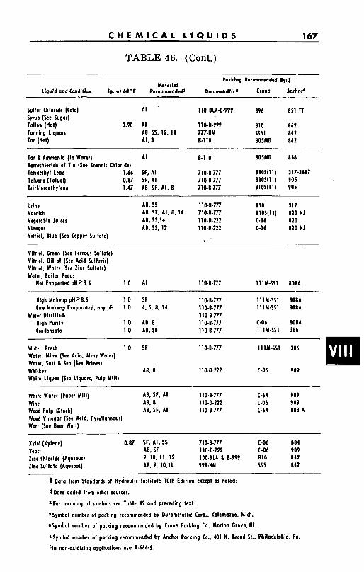
C H E M I C A L L I Q U I D S 167
TABLE 46. (Cont.)
Packing Recommend.d Byrx Moterial
Liquid and Condition le. at 6 0 - F Recommend41 Dummrbttic' Crone Anchor'
Sulfur Chloride (Cold) A I ' 110 BLA-8-999 896 8S1 n SYNP (See Sugar) Tallow (Hat) 0.90 AI 1104-222 810 862 Tonning Liquors AB, 55, 12, 14 777-NM 5161 842 Tar (Hat) AI, 3 B-110 8OSMD 842
Tar L Ammonia (In Water) Tetrachloride of Tin (See Stannic Chloride) Tetraethyl Lead 1.66 Toluene (Toluol) 0.87 Trichloroethylene 1.47
A I
SF, A I SF, A I AB, SF, AI, 8
8-110
710-8-777 710-8-777 710-8-777
8OSYO
a l o s ( l l ) 8105(11) 8lOS(ll)
856
317-3687 905 901
Urine Varnish Vegetable Julces Vinegar Vitriol, Blue (See Capper Sulfate)
AB. 55 AB, SF, AI, 8, 14 AB. 55.14 AB, 55, 12
110-8-777 710-8-777 110-0-222 110-0-222
810
(-06 (-06
e.lOS(11) 317 820 NJ 820 820 NJ
Vitriol, Green (See Ferrous Sulfate) Vitriol, O i l of (See Acid Sulfuric) Vitriol, White (See Zinc Sulfate) Water, Boiler Feed:
Not Evaparted pH>B.I 1.0 A I 110-8777 11 1M-SI1 808A
High Makeup pH>B.S 1.0 SF 110-8-777 11 1M-SI1 808A low Makeup Evoporated, any pH 1.0 4, I, 8, 14 110-8-777 11 1M-SS1 808A
Water Distilled: 110-8-777 High Purity 1.0 AB, 8 110-8-777 (-06 BORA Condensate 1.0 AB, SF i10-~-777 111M-SI1 386
Water, Fresh 1.0 SF 1104-777 111M-IS1 386 Water, Mine (See Acid, Mine Water) Watnr, Salt 6 Sea (See Brines) Whiskey AB, 8 110-0.222 (-06 909 White l iquor (Sea Liquors. Pulp Mill)
White Woter (Paper Mill) AB, SF. AI 110-8-777 (-64 909 Wine AB, 8 110-D-222 (-06 909 Wood Pulp ptock) AB, SF, AI i i o - r ~ - r n C-64 808 A Wood Vinegar (See Acid, Pyroligneous) Wort (See Beer Wort)
--
Xylol (Xylene) 0.87 SF. AI. SS 710.8-777 (-06 804 Yeast AB, SF 110-0-222 (-06 909 Zinc Chloride (Aqueous) 9, 10, 11, 12 100-BLA & 8-999 810 a42 Zinc Sulfate (Aqueous) AB, 9, 10.11 999-NM SI I 012
t Data from Standards of Hydraulic Institute 10th Edition except os noted:
*Data added from other sources.
=For meaning of symbols see Table 4s and preceding text.
*Symbol number of packing recommended by Durametallic Corp., Kalamazoo, Mich.
*symbol number of packing recommended by Crane Packing Co., Morton Crave, 111.
'Symbol number of pocking recommended by Anchor Packing Co., 401 N. Broad SI.. Philadelphia, Pa.
'In non-axidizing applicotianr use A-666-5
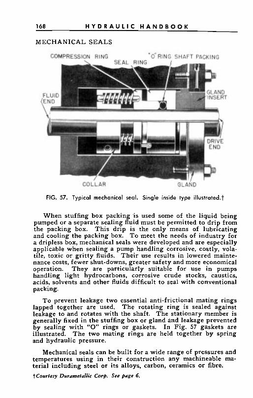
168 H Y D R A U L I C H A N D B O O K
MECHANICAL SEALS
FIG. 57. Typical mechanical seal. Single inside type il1ustroted.t
When stuffing box packing ,is used some of the liquid being pumped or a separate sealing fluid must be permitted to drip from the packing box. This drip is the only means of lubricating and cooling the packing box. T o meet the needs of industry for a dripless box, mechanical seals were developed and are especially applicable when sealing a pump handling corrosive, costly, vola- tile, toxic or grit ty fluids. Their use results in lowered mainte- nance costs, fewer shut-downs, greater safety and more economical operation. They are particularly suitable for use in pumps handling light hydrocarbons, corrosive crude stocks, caustics, acids, solvents and other fluids difficult to seal with conventional packing.
To prevent leakage two essential anti-frictional mating rings lapped together are used. The rotating ring is sealed against leakage to and rotates with the shaft. The stationary member is generally fixed in the stuffing box or gland and leakage prevented by sealing with “0” rings or gaskets. In Fig. 57 gaskets are illustrated. The two mating rings are held together by spring and hydraulic pressure.
Mechanical seals can be built for a wide range of pressures and temperatures using in their construction any machineable ma- terial including steel or its alloys, carbon, ceramics or fibre. t Courtesy Durametallic Corp. See page 6.
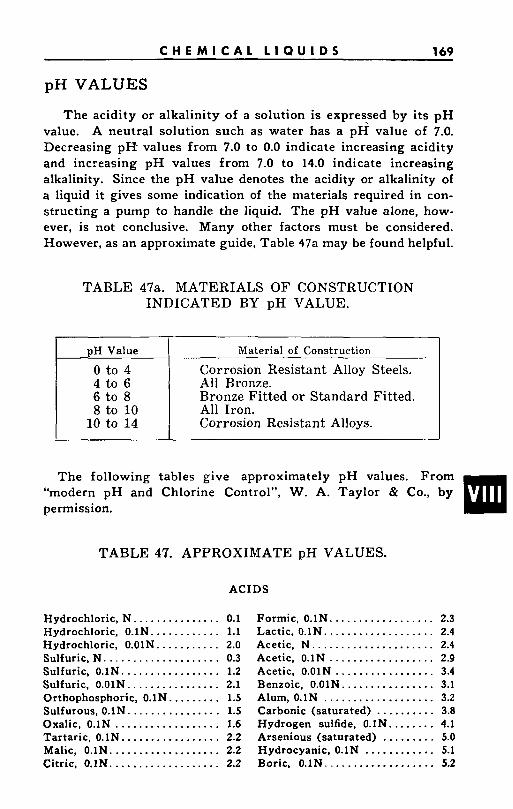
C H E M I C A L L I Q U I D S 1 69
~- pH Value
8 to 10 10 t o 14
pH VALUES
-- Material of Construction
Corrosion Resistant Alloy Steels. All Bronze. Bronze Fitted or Standard Fitted. All Iron. Corrosion Resistant Alloys.
The acidity or alkalinity of a solution is expressed by its p H value. A neutral solution such as water has a p H value of 7.0. Decreasing p R values from 7.0 to 0.0 indicate increasing acidity and increasing pH values from 7.0 to 14.0 indicate increasing alkalinity. Since the p H value denotes the acidity or alkalinity of a liquid it gives some indication of the materials required in con- structing a pump to handle the liquid. The pH value alone, how- ever, is not conclusive. Many other factors must be considered. However, as an approximate guide, Table 47a may be found helpful.
TABLE 47a. MATERIALS O F CONSTRUCTION INDICATED BY pH VALUE.
The following tables give approximately pH values. From “modern pH and Chlorine Control”, W. A. Taylor & Co., by permission.
TABLE 47. APPROXIMATE pH VALUES.
ACIDS
Hydrochloric, N . . ............. 0.1 Hydrochloric, 0.1N ............ 1.1 Hydrochloric, 0 .01N.. ......... 2.0 Sulfuric,N .................... 0.3 Sulfuric, 0 . 1 N . . ............... 1.2 Sulfuric, 0.01N ................ 2.1 Orthophosphoric, 0.1N. ........ 1.5 Sulfurous, O.1N. ............... 1.5 Oxalic, 0.1N .................. 1.6 Tartaric, 0 . 1 N . . ............... 2.2 Malic, 0 . 1 N . . ................. 2.2 Citric, 0 . 1 N . . ................. 2.2
Formic, 0.1N. ................. 2.3 Lactic, 0 . 1 N . . ................. 2.4 Acetic, N . . ................... 2.4 Acetic, 0 . 1 N . . ................ 2.9 Acetic, 0.01N ................. 3.4 Benzoic, 0.01N ................ 3.1 Alum, 0.1N ................... 3.2 Carbonic (saturated) .......... 3.8 Hydrogen sulfide, 0.1N. ....... 4.1 Arsenious (saturated) ......... 5.0 Hydrocyanic, 0.1N ............ 5.1 Boric. 0.1N. .................. 5.2
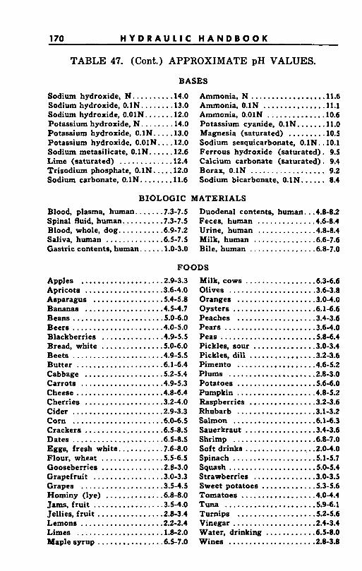
1 70 H Y D R A U L I C H A N D B O O K
TABLE 47 . (Cont.) APPROXIMATE pH VALUES . BASES
Sodium hydroxide. N ......... .1 4.0 Sodium hydroxide. 0.1N. ....... 13.0 Sodium hydroxide. 0.01N ...... .l 2.0 Potassium hydroxide. N ....... .l 4.0 Potassium hydroxide, 0.1N .... .l 3.0 Potassium hydroxide. 0.01N. . . . 12.0 Sodium metasilicate . 0.1N. .... .l 2.6 Lime (saturated) ............ .l 2.4 Trisodium phosphate . 0.1N. .... 12.0 Sodium carbonate, 0.1N ....... .l 1.6
Ammonia. N .................. 11.6 Ammonia. 0.1N .............. .1 1.1 Ammonia. 0.01N ............. .1 0.6 Potassium cyanide. 0.1N ...... .1 1.0 Magnesia (saturated) ........ .l 0.5 Sodium sesquicarbonate. 0.1N. . 10.1 Ferrous hydroxide (saturated) . 9.5 Calcium carbonate (saturated) . 9.4 Borax. 0.1N .................. 9.2 Sodium bicarbonate. 0.1N ...... 8.4
B I O L O G I C MATERIALS
Blood. plasma. human ...... .7.3. 7.5 Spinal fluid. human ......... .7.3. 7.5 Blood. whole. dog .......... .6.9. 7.2
Duodenal contents. human .. .4.8. 8.2 Feces . human ............. .4.6. 8.4 Urine. human ............. .4.8. 8.4
Saliva. human ............. .6.5. 7.5 Milk . human .............. .6.6. 7.6 Gastric contents. human ..... .l.O. 3.0 Bile. human ............... .6.8. 7.0
FOODS Apples ................... .2.9. 3.3 Milk. cows ................ .6.3. 6.6 Apricots .................. .3.6. 4.0 Olives .................... .3.6. 3.8 Asparagus ................ .5.4. 5.8 Oranges .................. .3.0. 4.0 Bananas .................. .4.5. 4.7 Oysters ................... .6.1. 6.6 Beans ..................... . S O . 6.0 Peaches .................. .3.4. 3.6 Beers ..................... .4.0. 5.0 Pears ..................... .3.6-4 .O Blackberries .............. .4.9. 5.5 Peas ...................... .5.8. 6.4
Beets ..................... .4.9. 5.5 Pickles, dill ............... .3.2. 3.6 Butter .................... .6.1. 6.4 Pimento .................. .4.6. 5.2 Cabbage .................. .5.2. 5.4 Plums .................... .2.8. 3.0 Carrots ................... .4.9. 5.3 Potatoes .................. .5.6. 6.0 Cheese .................... .4.8. 6.4 Pumpkin .................. .4.8. 5.2 Cherries .................. .3.2. 4.0 Raspberries ............... .3.2. 3.6 Cider ..................... .2.9. 3.3 Rhubarb .................. .3.1. 3.2 Corn ..................... .6.0. 6.5 Salmon ................... .6.1. 6.3 Crackers .................. .6.5. 8.5 Sauerkraut ................ .3.4. 3.6 Dates ..................... .6.5. 8.5 Shrimp ................... .6.8. 7.0 Eggs, fresh white .......... .7.6. 8.0 Soft drinks ................. .2.0 4.0 Flour. wheat .............. .5.5. 6.5 Spinach ................... .5.1. 5.7 Gooseberries .............. .2.8. 3.0 Squash .................... .5.0- 5.4 Grapefruit ................ .3.0. 3.3 Strawberries .............. .3.0. 3.5 Grapes ................... .3.5. 4.5 Sweet potatoes ............ .5.3. 5.6 Hominy (lye) ............. .6.8. 8.0 Tomatoes ................. .4.0-4 .4 Jams, f rui t ................ .3.5. 4.0 Tuna ..................... .5.9. 6.1 Jellies, f rui t ............... .2.8. 3.4 Turnips .................. .5.2. 5.6 Lemons ................... .2.2. 2.4 Vinegar ................... .2.4. 3.4 Limes .................... .1.8. 2.0 Water, drinking ........... .6.5. 8.0 Maple syrup ............... .6.5. 7.0 Wines .................... .2.8. 3.8
Bread. white .............. .SO. 6.0 Pickles, sour .............. .3.0. 3.4
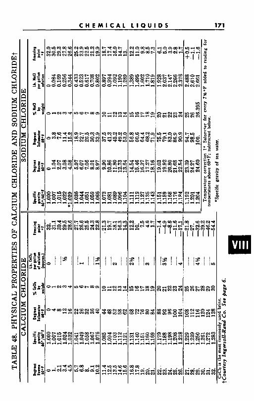
C H E M I C A L L I Q U I D S 171
+
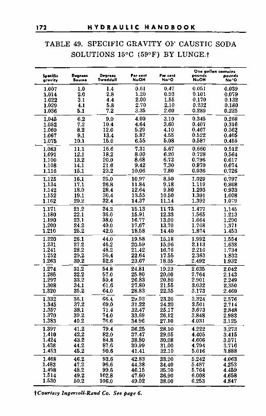
172 H Y D R A U L I C H A N D B O O K
TABLE 49. SPECIFIC GRAVITY OF CAUSTIC SODA SOLUTIONS 15OC (59OF) BY LUNGE.t
One gallon contains Specific Degrees Degrees Per cent Per cent pounds pounds gravity Baume lwaddell NaOH No20 NaOH NdO
1.007 1 .o 1.4 0.61 0.47 0.051 0.039 1.014 2.0 2.8 1.20 0.93 0.101 0.059 1.022 3.1 4.4 2.00 1.55 0.170 0.132 1.029 4.1 5.8 2.70 2.10 0.232 0.180 1.036 5.1 7.2 3.35 2.60 0.289 0.225 1.045 6.2 9.0 4.00 3.10 0.345 0.268 1 .052 7.2 10.4 4.64 3.60 0.407 0.316 - _ _ _ . ._ ~. - :::% 1.060 8.2 12.0 5.29 4.10 0.4G7 1.067 9.1 13.4 5.87 4.55 0.522 1.075 10.1 15.0 6.55 5.08 0.587 0.455 1.083 11.1 16.6 7.31 5.67 0.660 0.512 1.091 12.1 18.2 8.00 6.20 0.728 0.564 - . - -- - .~
1.100 13.2 20.0 8.68 6.73 0.796 0.617 1.108 14.1 21.6 9.42 7.30 0.8iO 0.674 1.116 15.1 23.2 10.06 7.80 0.936 0.726
.-
1.125 16.1 25.0 10.97 8.50 1.029 0.797 1.134 17.1 26.8 11.84 9.18 1.119 0.868 1.142 18.0 28.4 12.64 9.80 1.203 0.933 1.152 19.1 30.4 13.55 10.50 1.301 1.008 1.162 20.2 32.4 14.37 11.14 1.392 1.079 1.171 21.2 34.2 15.13 11.73 1.477 1.145 1.180 22.1 36.0 15.91 12.33 1.565 1.213 1.190 23.1 38.0 16.77 13.00 1.664 1.290 1.200 24.2 40.0 17.67 13.70 1.768 1.371 1.210 25.2 42.0 18.58 14.40 1.874 1.453 1.220 26.1 44.0 19.58 15.18 1.992 1.554 1.231 27.2 46.2 20.59 15.96 2.113 1.638 1.241 28.2 48.2 21.42 16.76 2.216 1.734 1.252 29.2 50.4 22.64 17.55 2.363 1.832 1.263 30.2 52.6 23.67 18.35 2.492 1.932 1.274 31.2 54.8 24.81 19.23 2.635 2.042 1.285 32.2 57.0 25.80 20.00 2.764 2.143 1.297 33.2 59.4 26.83 20.80 2.901 2.249 1.308 34.1 61.6 27.80 21.55 3.032 2.350 . i.320 35.2 64.0 28.83 22.35 3.173 2.460 1.332 36.1 6 c 4 29.93 23.20 3.324 2.576 1.345 37.2 69.0 31.22 24.20 3.501 2.714 1.357 38.1 71.4 32.47 25.17 3.673 2.848 1.370 39.2 74.0 33.69 26.12 3.848 2.983 1.383 40.2 76.6 34.96 27.10 4.031 3.125 1.397 41.2 79.4 36.25 28.10 4.222 3.273 1.410 42.2 82.0 37.47 29.05 4.405 3.415 1.424 43.2 84.8 38.80 30.08 4.606 3.671 1.438 44.2 87.6 39.99 31.00 4.794 3.716 1.453 45.2 90.6 41.41 32.10 5.016 3.888 - - -.- _ _ ~- . . ~ .
1.468 46.2 93.6 42.83 33.20 5.242 4.063 1.483 47.2 96.6 44.38 34.40 5.487 4.253 1.498 48.2 99.6 46.15 35.70 5.764 4.459 1.514 49.2 102.8 47.60 36.90 6.008 4.658 1.630 50.2 106.0 49.02 38.00 6.253 4.847
?Courtesy Zngersoll-Rand Co. See bage 6.
M E C H A N I C A L D A T A 173
SECTION IX-MECHANICAL DATA
CONTENTS
Page
Table-Dimensions Cast Iron Pipe.. .................................................... ..174 Table-Dimensions Cast Iron Flanged Fittings .................................. 175 TableDimensions Cast Iron Pipe Flanges .............................
Table-Roperties Steel and Wrought Iron Pipe ................................ ..177
Table-Weight and Dimensions of Copper and Brass Pipe and Tubes ...................................................................................... 1.
Table-Capacity of Vertical Cylindrical Tanks .................................. 181
Table-Horsepower of V-Belt Drives ...................................................... 182
Table-Functions of Numbers .................................................................. 183
Table-Capacity of Horizontal Cylindrical Tanks ............................. -181
Table-Pressure-Temperature Ratings for ASA Class 125 and Class 250 Pipe Flanges and Fittings ........................ 248
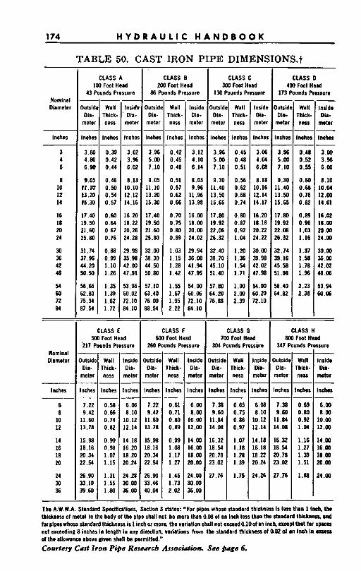
174 H Y D R A U L I C H A N D B O O K
TABLE 50. CAST IRON PIPE D1MENSIONS.t
jutside Dia-
meter
Inches
7.38 9.60
11.84 14.08
16.32 18.54 20.78 23.02
27.76
-- Wall
Thick- ness
Inches
0.65 0.75 0.86 0.97
1.07 1.18 1.28 1.39
1.75
-- --
Jutside Dia-
meter
Inches
7.22 9.42
11.60 13.78
15.98 18.16 20.34 22.54
26.90 33.10 39.60
Wall Thick. ness
Inches
0.58 0.66 0.74 0.82
0.90 0.98 1.07 1.15
1.31 1.55 1.80
-- -__
CLASS A I00 Foot Head
43 Pounds Pressure
CLASS c 300 foot Head
130 Pounds Pressure
C U S S D 400 Foot Head
I 7 3 Pounds Pressure
CLASS B 200 Foot Head
86 Pounds Pressure Nominal Diameter
- lnsidl Dia-
mete1
lnche
3.02 3.96 6.02
8.13 10.10 12.12 14.16
16.M 18.22 20.26 24.28
29.98 35.98 42.00 47.98
53.96 60.02 72.10 84.10
_.
-
- -
- Inside Dia-
metei
- Insidc Dia-
metel
Inchs:
3.06 4.04 6.08
- -
8.18 10.16 12.14 14.17
16.20 18.18 20.22 24.22
30.00 39.98 42.02 47.98
54.00 60.20 72.10
- -
- Outsid
Dia- meter
Inches
3.80 4.80 6.98
9-05
t3.20 15.30
17.40 19.50 21.60 25.80
31 .?4 37 .% 44.20 50.50
56.66 62.80 75.34 87 .54
- -
r 1 . m
- Wall
rhick ness
lnche
0.31 0.4i 0.44
0.a 0.N 0.54 0.51
0.60 0.64 0.67 0.76
0.88 0.99 1.10 1.26
1.35 1.39 I .62 1.72
-
-
Outsidl Dia-
meter
Wall rhick- ness
'nches
0.42 0.45 0.48
0.51 0.57 0.62 0.66
0.70 0.75 0.80 0.89
1.03 1.15 1.28 1.42
1.55 1.67 1.95 2.22
_.
-
Wall rhick- ness
riches
0.45 0.48 0.51
0.56 0.62 0.68 0.74
0.80 0.87 0.92 1.04
1.20 1.36 1.54 1.71
1.90 2.00 2.39
-
-
- -
Outside Dia-
meter
Inches
3 .96 5.00 7.10
9.30 11 .a 13.50 15.65
17.80 19.92 22 .ob 26.32
32.74 39.16 45.58 51.98
58.40 64.82
- -
- -
Wall Ihick- ness
riches
0.48 0.52 0.55
0.60 0.68 0.75 0.82
0.89 0.96 1.03 1.16
1.37 1.58 1.78 1.96
2.23 2.38
- -
- -
Inside Dia-
met8r
Inches -
Outsidi Dia-
meter
Inches
3.96 5.00 7.10
9.30 11.40 13.50 15.65
17.80 19.92 22.06 26.32
32.40 38.70 45.10 51.40
57.80 64.20 16.88
-
- -
~
Inches
3 4 6
8 10 I 2 I 4
16 18 20 24
30 36 42 4a
54 60 12 84
Inches
3.96 5.00 7.10
9.05 11.10 13.20 15.30
17.40 19.50 21.60 25.80
32.00 38.30 44.50 50.80
57.10 63.40 76.00 88.54
- lnche
3.12 4.1C 6.14
8.03 9.96
11.96 13.98
16.00 18.00 20.00 24.02
29.94 36.00 41.94 47 .%
54.00 60.06 72.10 84.10
__
- -
3.00 3.96 6.00
8.10 10.04 12.00 14.01
16.02 18.90 20.00 24.00
30.00 36.00 42.02 48.06
53.94 60.06
- - CLASS E
5W foot Head ,217 Pounds Pressure
CLASS F 600 Foot Head
260 Pounds Pressure
CLASS G 700 Foot Head
304 Pounds Pressure
C U S S H 800 Foot Hetd
347 Pounds P sure Nominal Diameter
- Inside Dia-
meter
lncher
6.06 8.10
10.12 12.14
14.18 16.20 18.20 20.24
24.28 30.00 36.00
- -
- Inside Dia-
meter
Inches -
- Inside Dia-
meter
Inches -
- Wall
Ihick- ness
Inches -
Outsid, Oia-
meter
lncha -
Wall rhick. ness
Inches _.
)ut s i d 1
Dia- meter
Inches -
Inside Dia-
meter
Inches -
Inches
6 8
10 12
14 16 18 20
24 30 36
7 2 2 9.42
11 .60 13.78
15.98 18.16 20.34 22.54
26.90 33.46 40.04
0.61 0.71 0.80 0.89
0.99 1.08 1.17 1.27
1.45 1.73 2.02
6.00 8.00
10.00 12.00
14.00 16.00 18.00 20.00
24.00 30.00 36.00
6.08 8.10
10.12 12.14
14.18 16.18 18.22 20.24
24.26
7.38 9.60
I1 .a4 14.08
16.32 I 8 54 20.78 23.02
27.76
0.69 0.80 0.92 1 .04
1.16 1.27 1.39 1.51
1.88
6.00 8.00
10.00 12.00
14.00 16.00 18.00 20.00
24.00
The A.W.W.A. Standard Specifications, Ssction 3 states: "for pipes whose standard thickness is less th8n 1 Inch, tbe thickness of metal i n the body of the plpe shall not be more than 0.08 of an inch less than the rt.ndrrd thickness, and for plpes whose standard thickness is I inch or more, the variation shall not erceed0.10of an inch, exceptthat for r- not exceeding 8 inches in length i n any direction. variations from the standard thickness of (LO2 ol 8n inch la ucds~ of the allowance above given shall be parmitted."
Courtesy Cat Zron Pipe Researcb A.rsocidiorr See page 6.
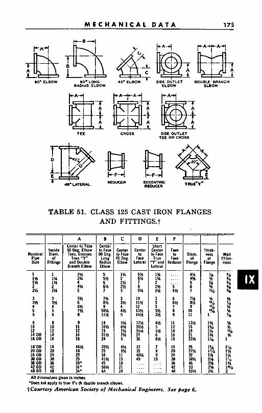
M E C H A N I C A L D A T A 175
Inside Diam.
of W n g s
1 1% 1% 2 2%
TEE
Center l o Face 90 Deg. Elbow Tees. Crosses
True "Y" and Double
Branch Elbow
3% 3% 4 4% 5
CROSS SIDE OUTLET TEE OR CROSS
Center 10 Face M Deg. Long
Radius Elbow
TABLE 51. CLASS 125 CAST IRON FLANGES AND F1TTINGS.t
Center lo Face 45 Deg Elbow
Nominal Pipe Size
1 1% 1% 2 2% 3 3% 4 5 6 8 10 12 14 OD 16 OD
180D 20 OD 24 OD 30 DD 36 OD 42 OD 48 OD
3 3% 4 5 6
8 10 12 14 16
A
5% 6 6% 7% 8
9 11 12 14 IS
::: 9
10% 11%
14 16% 19
I% 4% 5
5% 6% 7%
18 20 24 30 36 42 48
16% 18 22 25 28. 31. 34.
34 I1 41% 15 49 18 56% 21 64 24
Center I O
Face ateral
5% 6% 7 8 9%
10 11% 12 13% 14%
17% 20% 24% 27 30
32 35 40% 49
~
....
....
.... ~
- - E
Short Center to Face True
'Y'and Lateral
1% 1% 2 2% 2% 3 3 3 3% 3%
4% 5 5% 6 6%
7 8 9
-
-
10 . .... .... .... -
Face to
Face Reduce
- .... .... .... 5 5% 6
8 9
11 12 14 16 18
19 20 24 30 36 42 48
;%
--
Diam. of
Flange
4% 4% 5 6 7
7% 8% 9 10 11
13% 16 19 21 23% 25 27% 32 38% 46 53 59%
-
- All dimensions given i n inches,
*Does not apply l o true Yr Ut double branch elbows. tCowtesy American Society of Mechanical Engineers. See page 6.
-I- Thick-
Flange 1 ness
1% 1% 2% 1% 2% 1% 2% 1'!6 2% 2
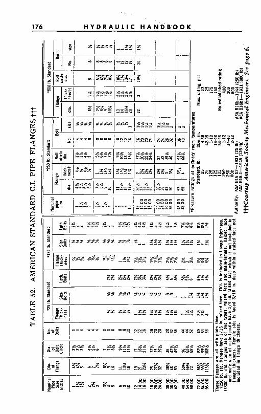
176 H Y D R A U 1 I C H A N D B'OO K
(Y
i - G
ZH s
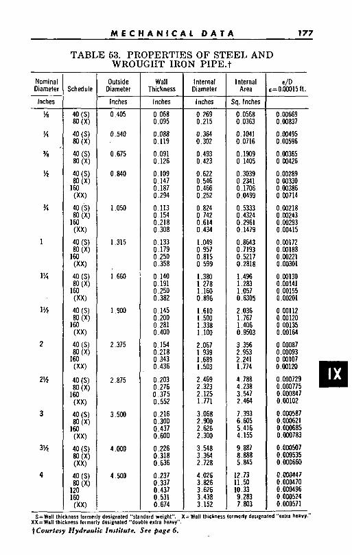
M E C H A N I C A L D A T A 177
TABLE 53. PROPERTIES O F STEEL AND WROUGHT IRON P1PE.t
Nominal Diameter
Inches
Schedule
L/s
?4
%
%
%
1
1%
1%
2
2%
3
3%
4
Outside I Wall Diameter Thickness
inches inches
0.405
0.540
0.675
0.840
1.050
1 315
1.660
1.900
2.375
2.875
3.500
4 .OOO
4.500
0.068 0.095
0.088 0.119
0.091 0.126
0.109 0.147 0.187 0.294
0.113 0.154 0.218 0.308
0.133 0.179 0.250 0.358
0.140 0.191 0.250 0.382
0.145 0.200 0.281 0.400
0.154 0.218 0.343 0.436
0.203 0.276 0.375 0.552
0.216 0.300 0.437 0.600 0.226 0.318 0.636
0.237 0.337 0.437 0.531 0.674
Internal Diameter
Inches
0.269 0.215
0.364 0.302
0.493 0.423
0.622 0.546 0.466 0.252
0 -824 0.742 0.614 0.434
1.049 0.957 0.815 0.599
1.380 1.278 1.160 0.896
1.610 1.500 1.338 1.100
2.067 1.939 1.689 1 503
2.469 2.323 2.125 1.771
3.068 2.900 2.626 2.300
3.548 3.364 2.728
4.026 3.826 3.626 3.438 3.152
Internal Area
Sq. Inches
0.0568 0.0363
0.1041 0.0716
0.1909 0.1405
0.3039 0.2341 0.1706 0.0499
0.5333 0.4324 0.2961 0.1479
0.8643 0.7193 0.5217 0.2818
1.496 1.283 1.057 0.6305
2.036 1.767 1.406 0.9503
3.356 2.953 2.241 1.774
4.788 4 238 3.547 2.464
7.393 6.605 5.416 4.155
9.887 8.888 5.845
12.73 11.50 10.33 9.283 7.803
0.00669 0.00837
0.00495 0.00596
0 00365 0 .00426
0.00289 0.00330 0 00386 0.00714
0.00218 0.00243 0.00293 0.00415
0.00172 0.00188 0.00221 0.00301
0.00130 0.00141 0.00155 0.00201
0.00112 0.00120 0.00135 0.00164
0.00087 0.00093 0.00107 0.00120
0.000729 0.000775 0.000847 0.00102
0.000587 0.000621 0.000685 0.000783
0.000507 0.000535 0.000660
0.000447 0.000470 0.000496 0.000524 0.000571
S= Wall thickness formerly designated "standard weight". X = Wall thickness lormerly designated "ertra heavy." X X = Wall thickness formerly designated "double extra heavy". $Courtesy Hydraulic Institute. See page 6.
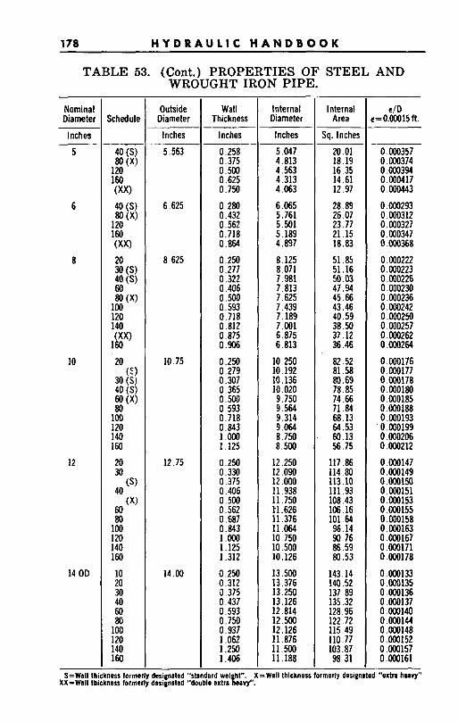
178 H Y D R A U L I C H A N D B O O K
TABLE 53. (Cont.) PROPERTIES OF STEEL AND WROUGHT IRON PIPE.
Outside Diameter
Inches
designated designated "double
Nominal Diameter
Wall Thickness
Inches -~
"standard wei ht" extra tsavr.'
Inches -
5
6
8
10
12
14 OD
S=Wall th XX-Wall thi
Schedule
5.563
6.625
8.625
10.75
12.75
14.00
0.258 0.375 0.500 0.625 0.750
0.280 0.432 0.562 0.718 0.864
0.250 0.277 0.322 0.406 0.500 0.593 0.718 0.812 0.875 0.906 0.250 0.279 0.307 0.365 0.500 0.593 0.718 0.843 1 .ooo 1.125 0.250 0.330 0.375 0.406 0.500 0.562 0.687 0.843 1 ,000 1.125 1.312 0.250 0.312 9.375 0.437 0.593 0.750 0.937 1.062 1.250 1.406
Internal Internal Diameter I Area
Inches 1 Sq. Inches
5.047 4.813 4.563 4.313 4.063 6.065 5.761 5.501 5.189 4.897 8.125 8.071 7.981 7.813 7.625 7.439 7.189 7.001 6.875 6.813 10.250 10.192 10.136 10.020 9.750 9.564 9.314 9 .OM 8.750 8.500 12.250 12.090 12 .wo 11.938 11.750 H .626 11.376 11.064 10.750 10.500 10.126 13.500 13.376 13.250 13.126 12.814 12.500 12.126 11.876 11.500 11.188
20.01 18.19 16.35 14.61 12.97 28.89 26.07 23.77 21.15 18.83 51.85 51.16 50.03 47.94 45.66 43.46 40.59 38.50 37.12 36.46 82.52 81.58 80.69 78.85 74.66 71.84 68.13 64.53 60.13 56.75 117.86 114.80 113.10 111.93 108.43 106.16 101.64 96.14 90.76 86.59 80.53
143.14 140.52 137.89 135.32 128.96 122.72 115.49 110.77 103.87 98.31
€/D e=0.00015 11.
0 000357 0 000374 0 000394 0 000417 0 000443 0 000293 0 000312 0 000327 0 000347 0 000368 0 000222 0 000223 0 000226 0 000230 0 000236 0 000242 0 000250 0 000257 0 000262 0 000264 0 000176 0 ooo177 0 000178 0 000180 0 000185 0 000188 0 000193 0 ooo199 0 000206 0 000212 0 000147 0 000149 0 oo0150 0 000151 0 000153 0 000155 0 000158 0 000163 0 000167 0 000171 0 000178 0 000133 0 000135 0 000136 0 000137 0 000140 0 OW144 0 000148 0 000152 0 000157 0 000161
led "extra heavy"
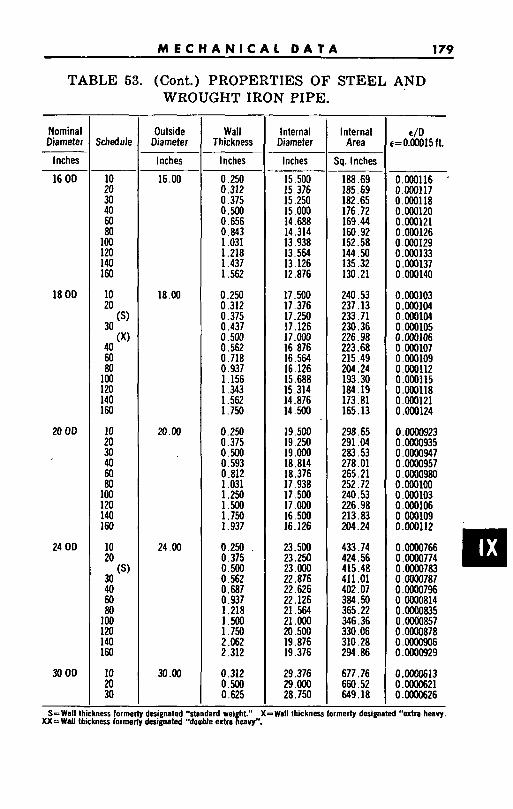
M E C H A N I C A L D A T A 179
TABLE 53. (Cont.) PROPERTIES OF STEEL AND
internal internal Diameter Area
inches Sq. Inches
WROUGHT IRON PIPE.
4 / D e=0.00015ft.
Nominal Diametei
inches
230.36 226.98 223.68 215.49 204.24 193.30 184.19 173.81 165.13
16 OD
18 OD
20 OD
24 OD
0 .000105 0.000106 0 .OO0107 0 .O00109 O.OOO112 0.000115 0.000118 0 .ooO121 0 .ooO124
Schedule
10 20 30 40 60 80
100 120 140 160
10 20
30
40 60 80
100 120 140 160
10 20 30 40 60 80
100 120 140 160
10 20
30 40 60 80
100 120 140 160
(SI
(XI
(S)
S- Wall thickness forme XX= W.U lhickness forme
Outside Diameter
Inches
16.00
18.00
20.00
24 .OO
30 .00
Wall Thickness
Inches
0.250 0.312 0.375 0.500 0.656 0.843 1.031 1.218 1.437 1.562
0.250 0.312 0.375 0.437 0.500 0.562 0.718 0.937 1.156 1.343 1.562 1.750
0.250 0.375 0.500 0.593 0.812 1.031 1.250 1.500 1.754 1.937
0 250 0.375 0.500 0.562 0.687 0.937 1.218 1 .500 1.750 2.062 2.312
0.312 0.500 0.625
designated "standard wei I designated "double extra fb;;".
15.500 15.376 15.250 15.000 14.688 14.314 13.938 13.564 13.126 12.876
17.500 17.376 17.250 17.126 17.000 16.876 16.564 16.126 15.688 15.314 14.876 14.500
19.500 19.250 19 ,000 18.814 18.376 17.938 17.500 17.000 16.500 16.126
23.500 23.250 23 ,000 22.876 22.626 22.126 21.564 21.000 20.500 19.876 19.376
188.69 185.69 182.65 176.72 169.44 160.92 152.58 144.50 135.32 130 21
0.000116 '
0.000117 0.000118 0 .m120 0.000121 0.000126 I o.Ooo129 O .oooii 0.000137 0 .OO0140
0 .ooo104 0 .Oo0104
298.65 291.04 283.53 278.01 265 21 252.72 240.53 226.98 213.83 204.24
433.74 424.56 415.48 411.01 402.07 384.50 365 2 2 346.36 330.06 310.28 294.86
0.0000766 0 .oooO774 0 .oooO783 0 .oooO787 0 .oooO796 0.0000814 0 .oooO&35 0 .oooO857 0 .oooO878 0 .oooO906 0 .Oo00929
29.376 677.76 0.0000613 29.Oo0 I 660.52 I O.oooO621 28.750 649.18 0.0000626
=Wall Ihickness formerly designated "extra heavy.
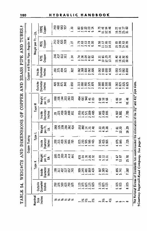
180 H Y D R A U L I C H A N D B O O K
I i L m 3 00 W L
al
z
-
I 2
E n
In v)
D c m
al CL n 0
L)
L
-
04 E n = - W
0 L)
n n
L ERE w o V
L FH w o 0
- m u L D N N W O N O N O 0 0 CQlnNO W h O N N w w o w o w o o 0 W N W O
" " 4 N c u m m u u m w ( . r w "15'9 : m 0.199? 9?9? 9149
I -
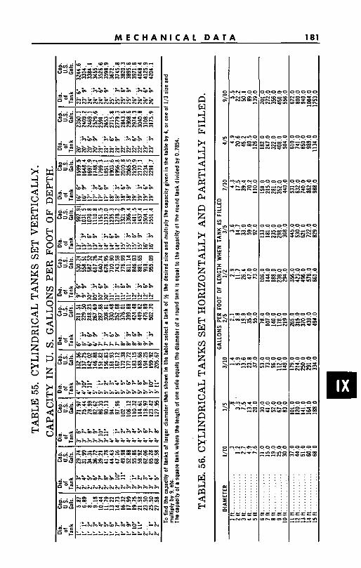
M E C H A N I C A L D A T A 181
I- f

182 H Y D R A U L I C H A N D B O O K
TABLE 57. V-BELT DR1VES.t
RECOMMENDED V-BELT CROSS-SECTIONS FOR VARIOUS HP. AND SPEEDS
575 490 ___
..................................
...................................
..................................
...................................
...................................
...................................
...................................
Horsepower 435
* )I
1 1% 2 3 5 7%
10 15 20 25 30 40 50 60 75
100 125 1M 200
1160 870
A A A A A A A A A A A B (or A)
B (or A) B B B B B o r C
B a r C C (or E) C (or B) C
C C C C
C o r D C o r D C o r D C o r D C o r D D ( o r 0
D (or C) D D D D D D 0 D D D D D D
--_ ----
250 300 and above
690
...........
...........
...........
~
. . .........
...........
...........
. . . . . . . . . . .
. . . . . . . . . . .
...........
........... D D D D D D D
D or E D o r E
E (or D) E E E
0 D D D D D
D (or E) E (or D) E (or D)
E
1750
A A A A A A
B (or A) B B B
B or C C (or B)
C C C C C C
___
..........
..........
..........
..........
..........
JTTE
Cross- iection
B
width W’ thic,k %
1.2 1.3 1.4 1.5 1.6 1.7
1.8 1.9 2.1 2.2 2.3
2.4 2.5 2.6 2.7 2.8
- -
-
-
......................
......................
...................... ........... ........... ........... ........... ...........
E E E E E
MOTOR SPEED-RPM
Velai ly in Feel
Per Minute --
_- lo00 1100 1200 1300 1400 1500 1600 1700 le00 1900 Moo
2100 2200 2300 2400 2500
Cross- Section
A
width %’
thick H’
.9 1.0 1.0 1.1 1.2 1.3
1.4 1.5 1.6 1.6 1.7
1.8 1.9 1.9 2.0 2.1
-
Cross- i g t i on
C
width K’
thick %*
Cross- Section
D
width 1%’ thick #’
--
3.0 3.2 3.4 3.6
4.0 3.13
-- 5.5 6 .0 6.5 7.0
8.0 7.5
5 BASED Velocity
Cross- in Feet Section Per
E Minute
4.3 4.6 4.9 5.2 5.5
thick
11 .o 3100
8.4 8.8 9.2 9.6
10.0
11.6 12.2 12.8 13.4 14.0
14.8 15.2 15.8 16.4 17.0
drive
3200 3300 34W 3500
3600 3700 3800 3900 4000 5000
5.7 5.9 6.1 6.3 6.5
10.5 11.0 11.5 12.0 12.5
E : I : E
............
............
............
............
. . . . . . . . . . . .
............
............
............ E E E E E E E E
N 180’ ARC OF CONTACT
A
width width width %’ zw H’
thick 1 ‘hi$ I thic,k %’ H
2.3 3.0 7.1 ::: 1 3”:: 1 ::: 2.5 I 3.3 I 7.7 2.5 3.4 7.9
22:; I 33:: I E 2.6 1 3.7 I 8.5
2.7 3.8 8.6 ::: I ::; I ::; 2.8 4.1 8.9 ::: I ::: 1 E
- - Cross- Section
D
width 1%’ thic,k #
12.9 13.3 13.7 14.1 14.5
14.8 15.1 15.4 15.7 16 .O
16.3 16.6 16.9 17.2 17.5 17.5
No. of belts required=- -- (hp per belt) (1- - ( ‘175(D-d’ C )
D=pitch diam. of large pulley, inches. d=pitch diam. of small pulley, inchar C=eenter distanca .inches. For pump. compressor and blower driver +Courtesy Dayton Rubber Manufacturing Co. See page 6.
more belting than shown by above formula should be used
- - Crms- iection
E
width 1%’ thick
1’
17.5 18.0 18.5 19.3 19.8
20 .o 20.5 21.0 21.3 21 .a 22.0 22.8 23.0 23.3 23.5 23.5
-
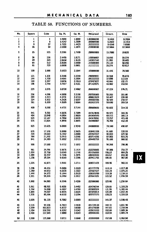
M E C H A N I C A L D A T A 183
Cu. Rl.
1.0000 1.2599 1.4423 1.5874
1.7100
1.8171 1.9129 2.0800 2.0801
2.1544
2.2240 2.2894 2.3513 2.4101
2.4662
TABLE 58. FUNCTIONS OF NUMBERS.
Reciprocal
1.000000000 .MOOD0000 .333333333 .250000000
.2OoM)wo
.I66666667
.142857143
.125000000
.111111111
.1000oOo00
.ow309091 ,083333333 ,076923077 .071428571
.OS6666667
Cube
2.6684
2.7144
2.7589 2.8020 2.8439 2.8845
2.9240
2.9625 3.MKw 3.0366 3.0723
3.1072
3.1414 3.1748 3.2075 3.23%
3.2711
3.3019 3.3322 3.3620 3.3912
3.4200
3.4482 3.4760 3.5034 3.5304
3.5569
3.5830
3.6342 3.6593
3.6840
3 . ~ 8 8
1 2 3 4
5
6 7 8 9
10
11 12 13 14
I 5
16 17 18 19
20
21 22 23 24
25
26 27 28 29
30
31 32 33 34
35
36 37 38 39
40
41 42 43 44
45
46 47 48 49
50
.OS2631579
.050000000
.047619048
.a45454545 ,043478261 1341666667
.04oowOW
,038461538 .037037037 .035714286 .034482759
.033333333
.032258065
.031250000
.ON303030
.OB411765
.028571429
,027777778 .027027027 ,026315789 ,025641026
.025000000
.024390244
.023809524 ,023255814 ,022727273
.022222222
.021739130
.020833333
.020408163
.02W000W
.02127ffim
1 4 9
16
25
36 49 64 81
100
121 144 169 1%
225
256 289 324 361
400
441 484 529 576
625
676 729 784 841
900
961 1.024 1.089 1.156
1.225
1.296 1,369 1.444 1.521
1.600
1.681 1,764 1.849 1.936
2.025
2,116 2.209 2,304 2.401
2,500
1 8
27 64
125
216 343 512 729
l.w
1.331 1.728 2.197 2.744
3.375
4,096 4,913 5.832 6.859
8,000
9.261 10,648 12.167 13.824
15.625
17.576 19.683 21.952 24.389
27.000
29,791 32.768 35.937 39.304
42.875
46.656 50.653 54.872 59.319
64.000
68.921 74.088 79.507 85.184
91.125
97,336 103.823 110,592 117,649
125,000
Sq. R t
1 .ow 1.4142 1.7321 2.0m
2.2361
2.4495 2.6458 2.8284 3.00w)
3.1623
3.3166 3.4641 3.6056 3.7417
3.8730
4 . m 4.1231 4.2426 4.3589
4.4721
4.5826 4.6904 4.7958 4.8990
5.0000
5.0990 5.1962 5.2915 5.3852
5.4772
5.5678 5.6569 5.7446 5.8310
5.9161
6.0000 6.0828 6.1644 6.2450
6.3246
6.4031 6.4807 6.5574 6.6332
6.7082
6.7823 6.8557 6.9282 7 . m
7.0711
2.5198 .062500000 2.5713 .OS8823529 2.6207 .OS5555556
Cirwm.
3.1416 6.2832 9.4248
12.5664
15.7080
18.850 21.991 25.133 28.274
31.416
34.558 37.699 40.841 43.982
47.124
50.265 53.407 56.549 59.690
62.832
65.973 69.115 72.257 75398
18.540
81.681 84.823 87.965 91.106
94.248
97.389 lOa53 103.67 106.81
109.96
113.10 116.24 119.38 122.52
125.66
128.81 131.95 135.09 138.23
141.37
144.51 147.65 150.80 153.94
157.08
Area
0.7854 3.1416 7.0686
12.5664
19.635
28.274 38.485 50266 63.617
78.540
95.033 113.10 132.73 153.94
176.71
201.06 226.98 254.47 283.53
314.16
346.36 380.13 415.48 45239
490.87
530.93 572.56 615.75 660.52
706.86
754.77 I . - ... .
855.30 907.92
962.11
1.017.88 1.07521 1.134.11 1.194.59
1.256.64
1.32025 1.385.44 1.452.20 1.520.53
1.590.43
1,661.90 1.734.94 1,809.56 1.885.74
1,963350
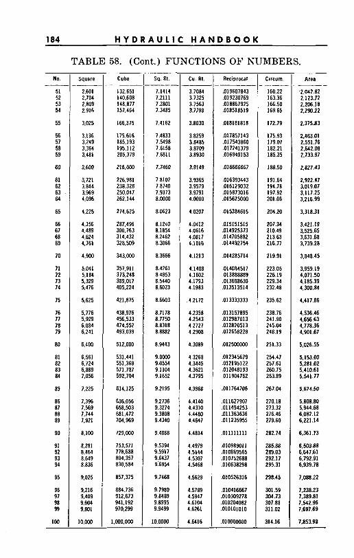
184 H Y D R A U L I C H A N D B O O K
TABLE 58. (Cont.) FUNCTIONS O F NUMBERS. -
No.
51 52 53 54
55
56 57 58 59
60
61 62 63 64
65
66 67 68 69
70
71 72 73 74
75
76 77 78 79
80
81 82 83 84
85
86 87 88 89
90
91 92 93 94
95
96 97 98 99
100
_- Square
2.601 2,704 2.809 2.916
3,025
3,136 3,249 3.364 3.481
3.600
3,721 3.844 3,969 4,096
4,225
4.356 4.489 4,624 4.761
4,900
5,041 5.184 5,329 5,476
5,625
5,776 5,929 6.084 6,241
6,400
6.561 6,724 6.889 7,056
7,225
7.396 7.569 7,744 7,921
8,100
8.281 8.464 8.649 8.836
9,025
9,216 9.409 9.604 9,801
10,000
___. Cube
132.651 140.608 148.877 157.464
166.375
175,616 185.193 195.112 205,379
216.000
226.981 238.328 250.047 262,144
274,625
287.496 300,763 314.432 328.509
343,000
357.911 373.248 389,017 405,224
421.875
438.976 456,533 474.552 493,039
512,000
531,441 551.368 571.787 592,704
614,125
636,056 658.503 681.472 704.969
729,000
753,571 778,688 804.357 830,584
857.375
884.736 912.673 941.192 970,299
1,000,000
~___ sq. ut.
7.1414 7.2111 7.2801 7.3485
7.4162
7.4833 7.5498 7.6158 7.6811
7.7460
7.8102 7.8740 7.9373 8.0000
8.0623
8.1240 8.1854 8.2462 8.3066
8.3666
8.4261 8.4853 8.5440 8.6023
8.6603
8.7178 8.7750 8.8318 8.8882
8.9443
9.0000 9.0554 9.1104 9.1652
9.2195
9.2736 9.3274 9.3808 9.4340
9.4868
9.5394 9.5917 9:6437 9.6954
9.7468
9.7980 9.8489 9.8995 9.9499
10.0000
cu. ut.
3.7084 3.7325 3.7563 3.7798
3.8030
3.8259 3.8485 3.8709 3.8930
3.9149
3.9365 3.9579 3.9791 4.0000
4.0207
4.0412 4.0616 4.0817 4.1016
4.1213
4.1408 4.1602 4.1793 4.1983
.4.2172
4.2358 4.2543 4.2727 4.2908
4.3089
4.3268 4.3445 4.3621 4.3795
4.3968
4.4140 4.4310 4.4480 4.4647
4.4814
4.4979 4.5144 4.5307 4.5468
4.5629
4.5789 4.5947 4.6104 4.6261
4.6416
-- Reciprocal
.019607843 ,019230769 .018867925 .018518519
.018181818
.017857143 ,017543860 ,017241379 .016949153
,016666667
.016393443
.016129032
.015873016
.015625000
,015384615
.015151515 ,014925373 .014705882 ,014492754
.014285714
.014084517
,013698630 ,013513514
,013333333
.013157895
.012987013
.012820513
.012658228
.012500000
,012345679 .012195122 .012048193 .011904762
.011764706
.011627907 ,011494253 ,011363636 .011235955
.011111111
.010989011 ,010869565 ,010752688 .010638298
,010526316
.010416667
.010309278
.010204082
.010101010
.o100owoo
.013~a8889
Circum.
160.22 163.36 166.50 169.65
172.79
175.93 179.07 182.21 185.35
188.50
191.64 194.78 197.92 201.06
204.20
207.34 210.49 213.63 216.71
219.91
223.05 226.19 229.34 232.48
235.62
238.76 241.90 245.04 248.19
251.33
254.47 257.61 260.75 263.89
267.04
270.18 273.32 276.46 279.60
282.74
285.88 289.03 292.17 295.31
298.45
301.59 304.73 307.88 311.02
314.16
. Area
.2.042.82 2,123.72 2.206.18 2,290.22
2.375.83
2.463.01 2.551.76 2.W2.08 2.733.97
2.827.43
2,92217 3.01 9.07 3.117.25 3.216.99
3.318.31
3,421.19 3.525.65 3,631.68 3.739.28
3.848.45
3,959.19 4.071.50 4.185.39 4.300.84
4.417.86
4,536.46 4.656.63 4.778.36 4,901.67
5,026.55
5.153.00 5.281.02 5.410.61 5.541.77
5.674.50
5.808.80 5.944.68 6,082.12 6,221.14
6,361.73
6,503.88 6,647.61 6,792.91 6.939.78
7.088.22
1.238.23 7.389.81 7,542.96 7,697.69
7.853.98
E L E C T R I C A L D A T A 185
SECTION X-ELECTRICAL DATA
CONTENTS
Page
Electric Motors-Service Conditions . . . . . . . . . . . . . . . . . . . . . . . .186 Electric Motors-Characteristics . . . . . . . . . . . . . . . . . . . . . . . + . . . .1%7 Electric Motors-Synchronous Speeds . . . . . . . . . . . . . . . . . . , . . . .187
Electric Circuits-Formula . . . . . . . . . . . . . . . . . . . . . . . . . . . . , . . . .188 Electric Motors-Full Load Currents. . . . . . . . . . . . . . . . . . . , . . . .189 Watt Hour Meters-Disc Constants and Horsepower
Formula . . . . . . . . . . . . . . . . . . . . . . . . . . . . . . . . . . . . . . . . . . , . . . .190 Electric Circuits-Wire and Fuse Sizes. . . . . . . . . . . . . . . . . . . . . . .192
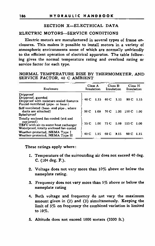
186 H Y D R A U L I C H A N D B O O K
SECTION X-ELECTRICAL DATA
ELECTRIC MOTORS-SERVICE CONDITIONS
Electric motofs are manufactured in several types of frame en- closures. This makes it possible to install motors in a variety of atmospheric environments some of which are normally unfriendly to the efficient operation of electrical apparatus. The table follow- ing gives the normal temperature rating and overload rating or service factor for each type.
NORMAL TEMPERATURE RISE BY THERMOMETER, AND SERVICE FACTOR, 40 C AMBIENT
Class A Class B Class H Enclosure Insulation Insulation Insulation
40C 1.15 60C 1.15 9OC 1.15 I Dripproof
Dripproof, guarded Dripproof with moisture-sealed features Forced-ventilated (pipe- or base-) Self-ventilated (base- and pipe-, where
Splashproof Totally enclosed fan-cooled (std and
1 ducts are attached) J 50 C 1.00 70 C 1.00 110 C 1.00
1 exp-proof)
TEFC with air-to-water heat exchanger } 55 '.O0 75 "O0 '15 '.O0 Waterproof, totally enclosed fan-cooled J
9OC 1.15 Weather-protected, N E M A Type I Weather-protected. N E M A T v w I1 } 4 0 C 1.15 60C B.15
These ratings apply where:
1.
2.
3.
4.
5.
Temperature of the surrounding air does not exceed 40 deg. C. (104 deg. F.).
Voltage does not vary more than 10% above or below the nameplate rating.
Frequency does not vary more than 5% above or below the nameplate rating
Both voltage and frequency do not vary the maximum amount given in (2) and (3) simultaneously. Keeping the limit of 5% on frequency the combined variation is limited to 10%.
Altitude does not exceed 1000 meters (3300 ft.)
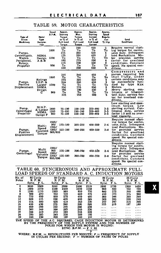
E L E C T R I C A L D A T A 187
TABLE 59. MOTOR CHARACTERISTICS
150-160 150-160 150-160
1800/ Multi- lz::l 125-180
Pumps. c ~ $ ~ ~ n t 1200/ 125-180 Positive Torque 900/600
Displacement
200-250
200-250
Low starting and max- imum torque. Low
350-400 3-5 starting current. Con- 350-400 3-5 tinuous duty, service 350-400 3-5 factor 1.0 and no over-
load capacity. Require normal sbr t - ing torque for contin-
450-550 2-4 uous. duty. Infrequent load fluctuations. ~ M o -
450-550 2-4 tor provides service factor for overload conditions. Constant speed. No special con-
Require normal start- ing torque for contin- uous duty. Infrequent
Pumps. ‘98:;’ 125-180 200-250 450-550 2-4 load fluctuations. Mo- Centrifugal Speed 1800/ tor provides service
Variable 1200/ 125-180 200-250 450-550 2-4 factor for overload Torque 900/600 conditions. Constant
speed. No special con- ditions.
WHERE: R.P.M. = REVOLUTIONS PER MINUTE: F = FREQUENCY OF SUPPLY IN CYCLES PER SECOND; P = NUMBER OF PAIRS OF POLES
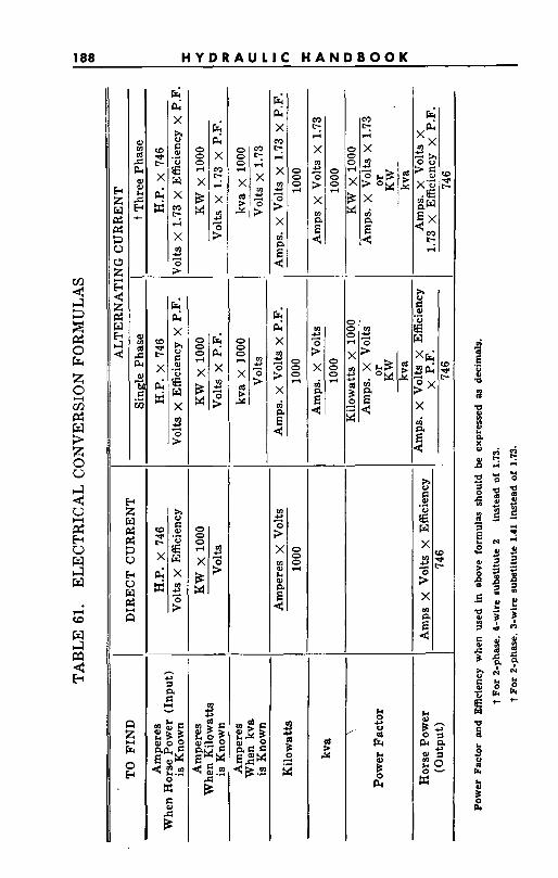
188 H Y D R A U L I C H A N D B O O K
W " c1
X
X a
W " c- X
X a
W -3 c1
X
X a
h U 7 a E U v
0 0 0 rl
X
w B
a c X
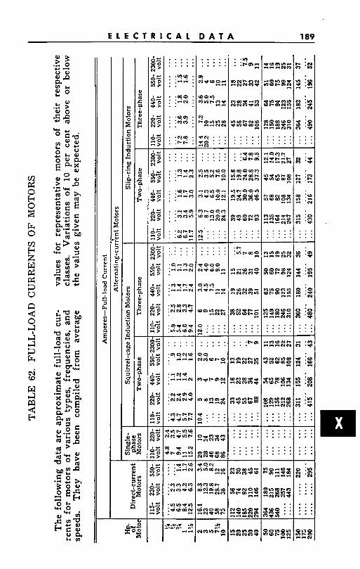
E L E C T R I C A L D A T A 189
. . . . . . . . . . . . . . . . . . . . . . . . . . . . . .
. :*c9 : : . t - C - .
. . . . . . . . . . . . . . .
W N . . . -N e o : : :
. . . . . . . . . . . . . . .
ZW%SZ ?s$; f rg . . . . . . . . . . . . . . . . . . . . . . . . . . . . . . . . . . . . . . . . . .bo, -mwPah - .m . . 0 *e
2ul'MEZ se22: 5 1s ZWSXZ S%%$ ; :g 3 $ 9 E I gg%c!S =: :2
---NN C 9 0 . . . . . . . . . . . . . . . . . . . . . . . . . . . . . . . . . . . . . . . . . . . . . . . . . . . . . . . . . . . . . . . . . . . . . . . . . . . . . . . . . . . . . . . . . . . . . . . . . . . . . . . . . . . . . . . . . . . . .
;4g$'6 Fz:=S!2 :: N 1: . . . --
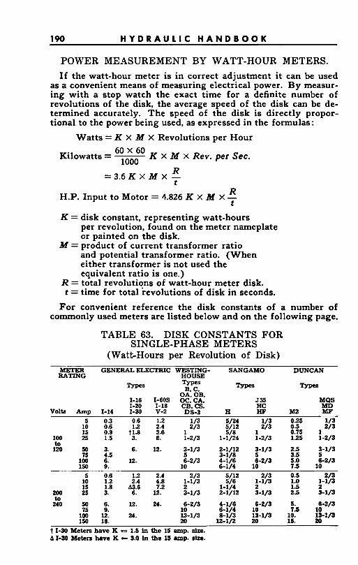
190 H Y D R A U L I C H A N D B O O K
POWER ME-4SUREMENT BY WATT-HOUR METERS.
If the watt-hour meter is in correct adjustment it can be used as a convenient means of measuring electrical power. By measur- ing with a stop watch the exact time for a definite number of revolutions of the disk, the average speed of the disk can be de- termined accurately. The speed of the disk is directly propor- tional to the power being used, as expressed in the formulas :
Watts = K X M X Revolutions per Hour
Kilowatts = ~ 6o 6o K x M X Rev. per Sec. 1000
R = 3 . 6 K x M x - t
R H.P. Input to Motor = 4.826 K X M X - t
K = disk constant, representing watt-hours per revolution, found on the meter nameplate or painted on the disk.
M = product of current transformer ratio and potential transformer ratio. (When either transformer is not used the equivalent ratio is one.)
R = total revolutions of watt-hour meter disk.
For convenient reference the disk constants of a number of commonly used meters are listed below and on the following page.
r = time for total revolutions of disk in seconds.
-___ METER RATING
Volts Amp 5
10 15
I00 25
TABLE 63. DISK CONSTANTS FOR
( Watt-Hours per Revolution of Disk) SINGLE-PHASE METERS
GENERAL ELECTRIC WESTING- SANGAMO HOUSE Types B. C.
OA OB, Types Types
1-16 1-60s 0C:CA. 535 1-20 1-18 CB. CS. HC
1-14 1-30 V-2 DS-3 H HF 0.3 0.6 1.2 1/3 5/24 1/3 0.6 1.2 2.4 2/3 5/12 2/3 0.9 71.8 3.6 1 5/8 1 1.5 3. 6. 1-2/3 1-1/24 1-2/3
DUNCAN
Types
MQS MD
M2 MF 0.25 1/3 0.5 2/3 0.75 I 1.25 1-2/3
to 120 50 3. 6. 12. 3-1/3 2-1/12 3-1/3 2.5 3-1/3
75 4.5 5 3-1/8 5 3.5 5 100 6. 12. 6-2/3 4-1/6 6-2/3 5.0 6-2/3 150 9. 10 6-1/4 10 7.5 10
5 0.6 1.2 2.4 2/3 5/12 2/3 0.5 2/3 10 1.2 2.4 4.8 1-1/3 15 1.8 A3.6 7.2 2 1-1/4 2 1.5 2
5/6 1-1/3 1.0 1-1/3
200 25 3. 6. 12. 3-1/3 2-1/12 3-1/3 2.5 3-1/3 to
240 50 6. 12. 24. 6-2/5 4-1/6 6-2/3 5. 6-2/3
100 12. 24. 13-1/3 8-1/3 13-1/3 IO. 19-1/9 75 9. 10 6-1/4 10 7.5 10
I50 18. 20 12-1/2 20 15. 20 t 1-30 Meters have K A 1-30 Metera have K
1 5 in the 15 amp. size. 3.0 in the 15 amp. &a.
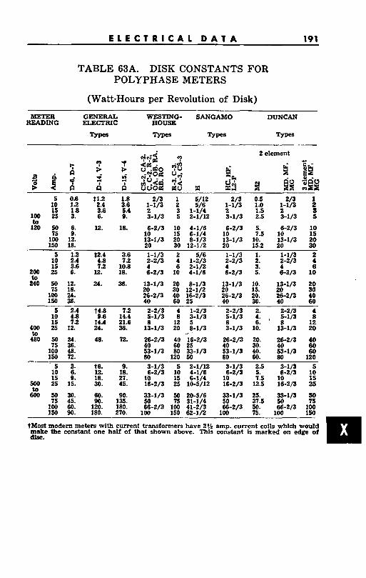
E L E C T R I C A L D A T A 191
TABLE 63A. DISK CONSTANTS FOR POLYPHASE METERS
(Watt-Hours per Revolution of Disk) METER GENERAL WESTING- SANCAMO DUNCAN
READING ELECTRIC HOUSE
Types m s Types Types - .-
5 0.6 1.8 2/3 1 5/12 2/3 0.5 2/3 1 10 1.2 % 3.6 1-1/3 2 5/6 1-1/3 1.0 1-1/3 2 15 ia 3.6 5.4 2 3 1-1/4 2 1.5 2 3
100 25 3. 6. 9. 3-1/3 5 2-1/12 3-1/3 2.5 3-1/3 5 ta 120 50
75 100 150
6. 12. 18. 6-2/3 10 4-1/6 9. 10 15 6-1/4
12. 13-1/3 20 8-1/3 18. 20 30 12-112
6-2/3 5. 6-2/3 10 10 7.5 10 15 13-1/3 10. 13-1/3 20 20 15.2 20 30
5 10 15 ?? 25
12 t2.4 3.6 1-1/3 2 5/6 1-1/3 1. 1-1/3 2 2.4 4.8 7.2 2-2/3 4 1-2/3 2-2/3 2. 2-2/3 4 3.6 7.2 10.8 4 6 2-1/2 4 3. 4 6 6. 12. 18. 6-2/3 10 4-1/6 6-2/3 5. 6-2/3 10
GO 50 12. 24. 36. 13-1/3 20 8-1/3 13-1/3 10. 13-1/3 20 75 18. 20 30 12-1/2 20 15. 20 30
100 24. 26-2/3 40 16-2/3 26-2/3 20. 26-2/3 40 150 36. 40 60 25 40 30. 40 60 --
5 2.4 t4.8 7 2 2-2/3 4 1-2/3 2-2/3 2. 2-2f3 4 io 4 8 9.6 14.4 5-113 1; g-113 5-113 4. 5-113 a 15 7 2 14.4 21.6 8 8 6. * 8 12
400 25 12. 24. 36. 13-1/3 20 8-1/3 3-1/3 10. 13-1/3 20 to 480 50
75 100 150 ___
5 10 15 25
24. 36. 48. 72. 3. 6. 9.
15.
48.
t6. 12. 18. 30.
12.
9. 18. 27. 45.
.r
26-2/3 40 16-2/3
53-1/3 80 33-1/3 40 60 25
80 120 50 3-1/3 5 2-1/12 6-2/3 10 4-1/6
10 15 6-1/4 16-2/3 25 10-5/12
26-2/3 40 53-1/3 80 3-1/3 6-2/3
10 16-2/3
20. 30. 40. 60. 2.5 5. 7.5
12.5
26-2/3 40 53-113 80 3-113 6-2/3
10 16-2 f3
40 Bo 60
120 - 5
10 15 25
600 50 30. 60. 90. 33-1/3 50 20-5/6 33-1/3 25. 33-1/3 50 75 45. 90. 135. 50 75 31-1/4 50 37.5 50 75
100 60. 120. 180. 66-2/3 100 41-2/3 66-2/3 50. 66-213 100 150 90. 180. 270. 100 150 62-1/2 100 75. 100 150
El tMost modem meters with current transformers have 2!5 amp. current coils which would make the constant one half of that shown above. This constant is marked on edge of disc.
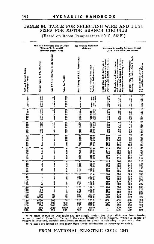
192 H Y D R A U L I C H A N D B O O K
TABLE 64. TABLE FOR SELECTING WIRE AND FUSE SIZES FOR MOTOR BRANCH CIRCUITS (Based on Room Temperature 30°C. 86°F.)
Minimum Allowoble Size of Copper Wire, A. W. C. or MCM Notional Electric Code
For Running Protection of Motors Moximum Allmwoblc Rating o f Branch.
Circuit Fuses with Code Letters
1 14 14 14 2 1.25 15 15 15 15 2 14 14 14 3 2.50 15 15 15 15 3 14 14 14 4 3.75 15 15 15 15 4 14 14 14 6 5.0 15 15 15 15 5 14 14 14 8 6.25 15 15 15 15
8 14 14 14 10 10.0 25 20 20 15 10 14 14 14 15 12.50 30 25 20 15
15 15.00 40 30 25 20 12 14 14 14 14 14 12 14 20 17.50 45 35 30 25 16 12 12 14 20 20.00 18 12 12 14 25 22.50 60 45 40 30 20 12 12 14 25 25.0 60 50 40 30
30 30.0 80 60 50 40 24 10 10 14 90 70 60 45 28 10 10 12 35 35.0
32 8 8 10 40 40.0 100 80 70 50 36 8 8 10 45 45.0 100 90 80 60 40 8 8 10 50 50.0 125 100 80 60 44 6 8 8 60 55.0 125 110 90 70
150 125 100 80 48 6 6 8 60 60.0 6 - 70-65.0 52
56 4 6 6 70 70.0 175 150 120 90 60 4 6 6 80 75.0 200 150 120 90 64 4 6 6 80 80.0 200 175 150 100 68 4 4 6 90 85.0 225 175 150 110
76 3 4 4 100 95.0 250 200 175 125 80 3 4 4 100 100.0 250 200 175 125
2 4 4 110 105.0 250 225 175 150 84 300 225 200 150 88 2 3 4 110 110.0
96 1 3 3 125 120.0 300 250 200 150 1 3 3 125 125.0 300 250 200 150 100
110 1 2 2 150 137.5 350 300 225 175 400 300 250 200 150 150.0 400
120 0 1 2 00 1 1 175 162.5
450 350 300 225 140 00 0 1 175 175.0 200 187.5 450 400 300 225 150 000 0 0
00 200 200.0 500 400 350 250 225 213.0 500 450 350 300
600----.450---460 -300-
160 000 170 0000 00
00 225 225.0 600 500 400 300
-iSF 0000 000 190 0000 000 000 250 238.0
250 0000 000 250 250.0 600 500 400 300 300 275.0 ... 600 500 400
. _ . 600 500 400 220
300 300.0 300 0000 0000
240 300 250 250
6 14 14 14 8 7.50 20 15 1 5 1 5 -
50 -40-35-- 25 --
--
175 - i50110 -
72 3 4 h 9 0 90.0 225 200 150-.--lTO-
..-2.so-.oo _ _ -150 .. -92 2 3 3- ----i25 115.0 300
200 . .... 3503-o.o. - . __ -1-30
O0 00 __ _. ____
Wire sizes shown In this table are for single motor. for short distances from feeder center to motor. therefore the wire sizes are tabulated as minimum. Where a group of motors is involved. special consideration must be given in selecting proper wire size.
Wire sizes are based on not more than three conductors in raceway or cable.
FROM NATIONAL ELECTRIC CODE 1947
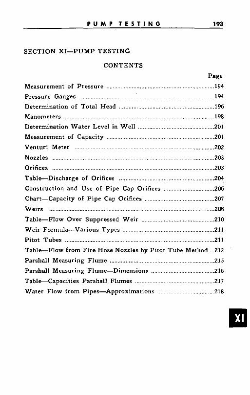
P U M P T E S T I N G 193
SECTION XI-PUMP TESTING
CONTENTS
Page
Measurement of Pressure .............................. ..194
Pressure Gauges .................................................................................... 194
Determination of Total Head ............ . .............................................. 196
Manometers ............................................................................................... 198
Determination Water Level in Well .................................... Measurement of Capacity .
Venturi Meter ...........................................................
Nozzles ........ .... .. . .. ... . .. . .. . . ..... . .... . ... . . . . . . . . . . . .. . . . . . . . . . . . . . . . . . . Orifices ...................................................................................................... 203
Table-Discharge of Orifices ............................................................ 204
Construction and Use of Pipe Cap Orifices ......
Chart-Capacity of Pipe Cap Orifices ............................................ 207
Weirs ......................................................................................................... ~ 0 8
Table-Flow Over Suppressed Weir .............................................. 210
Weir Formula-Various Types ........................................................... 211
Pitot Tubes ...................................................................... ................ 211
Table-Flow from Fire Hose Nozzles by Pitot Tube Method .... 212
Parshall Measuring Flume ................................................................... 215
Parshall Measuring Flume-Dimensions ........................................ 216
Table-Capacities Parshall Flumes .................................................. 217
Water Flow from Pipes-Approximations .................................... 218
n
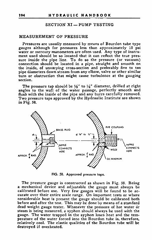
194 H Y D R A U L I C H A N D B O O K
SECTION XI - P U M P TESTING
MEASUREMENT OF PRESSURE
Pressures are usually measured by means of Bourdon tube type gauges although for pressures less than approximately 10 psi water or mercury manometers are often used. Any type of instru- ment used should be so located that it can reflect the true pres- sure inside the pipe line. T o do so the pressure (or vacuum) connection should be located in a pipe, straight and smooth on the inside, of unvarying cross-section and preferably five to ten pipe diameters down stream from any elbow, valve or other similar turn or obstruction that might cause turbulence a t the gauging section.
to f /4" diameter, drilled at right angles to the wall of the water passage, perfectly smooth and flush with the inside of the pipe and any burrs carefully removed. Two pressure taps approved by the Hydraulic Institute are shown in Fig. 58.
The pressure tap should be
APPROX.
NIPPLE CONNECTS HERE
9 4
FIG. 58. Approved pressure taps.
The pressure gauge is constructed as shown in Fig. 59. Being a mechanical device and adjustable the gauge must always be calibrated before use. Very few gauges will be found to be ac- curate over their entire scale range. On important tests or where considerable heat is present the gauge should be calibrated both before and after the test. This may be done by means of a standaTd dead weight gauge tester. Whenever the pressure of hot water or steam is being measured, a syphon should always be used with the gauge. The water trapped in the syphon loses heat and the tem- perature of the water forced into the Bourdon tube is, therefore, relatively cool. The elastic qualities of the Bourdon tube will be destroyed if overheated.
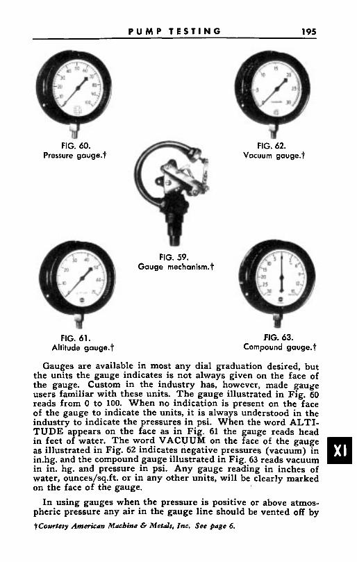
P U M P T E S T I N G 195
FIG. 60. Pressure gauge. t
FIG. 62. Vacuum gauge.t
FIG. 59. Gauge mechani5m.t
FIG. 61. Altitude gauge.t
FIG. 63. Compound gauge.1
Gauges are available in most any dial graduation desired, but the units the gauge indicates is not always given on the face of the gauge. Custom in the industry has, however, made gauge users familiar with these units. The gauge illustrated in Fig. 60 reads from 0 to 100. When no indication is present on the face of the gauge to indicate the units, it is always understood in the industry to indicate the pressures in psi. When the word ALTI- T U D E appears on the face as in Fig. 61 the gauge reads head in feet of water. The word VACUUM on the face of the gauge as illustrated in Fig. 62 indicates negative pressures (vacuum) in in.hg. and the compound gauge illustrated in Fig. 63 reads vacuum in in. hg. and pressure in psi. Any gauge reading in inches of water, ounces/sq.ft. or in any other units, will be clearly marked on the face of the gauge.
I n using gauges when the pressure is positive or above atmos- pheric pressure any air in the gauge line should be vented off by ?Courtesy American Macbine 6 Metals, Inc. See page 6.
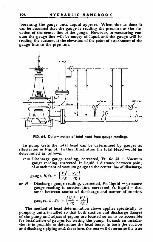
1 96 H Y D R A U L I C H A N D B O O K
loosening the gauge until liquid appeprs. When this is done it can be assumed that the gauge is reading the pressure at the ele- vation of the center line of the gauge. However, in measuring vac- uum the gauge line will be empty of liquid and the gauge will be reading the vacuum at the elevation of the point of attachment of the gauge line to the pipe line.
FIG. 64. Determination of total head from gauge readings.
In pump tests the total head can be determined by gauges as illustrated in Fig. 64. I n this illustration the total Head would be determined as follows. H = Discharge gauge reading, corrected, Ft. liquid + Vacuum
gauge reading, corrected, ft . liquid + distance between point of attachment of vacuum gauge to the center line of discharge
or H = Discharge gauge reading, corrected, Ft . liquid - pressure gauge reading in suction line, corrected, ft. liquid + dis- tance between center of discharge and center of suction
gauges, h, Ft. + - - - (1: 1;) The method of head determination above applies specifically to
pumping units installed SO th& both suction and discharge flanges of the pump and adjacent piping are located so as to be accessible for installation of gauges for testing the pump. In such an installa- tion it is possible to determine the head losses in both the suction and discharge piping and, therefore, the test will determine the true
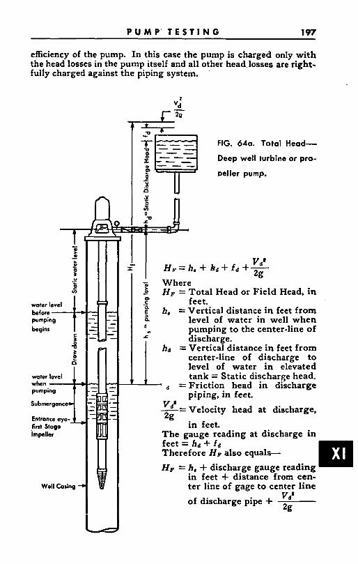
P U M P' T E 5 T I N G 197
efficiency of the pump. In this case the pump is charged only with the head losses in the pump itself and all other head.losses are right- fully charged against the piping system.
- 0
0 - L .. g .- .. 0
woter level
pumping before i begins
5 0 t e
woter level
Submergenc
Entrance eye- first Stoge Impeller
Well Caring -
+
FIG. 64a. Total Head-
Deep well turbine or pro-
Deller pump.
4 Where 3 Hp = Total Head or Field Head, i n
feet. E h, = Vertical distance in feet from 2 level of water in well when
x discharge.
m .-
II " pumping to the center-line of
ha = Vertical distance in feet from center-line of discharge to level of water in elevated tank = Static discharge head.
4 =Friction head in discharge piping, in feet.
-= Velocity head at discharge,
in feet. 2g
The gauge reading at discharge in feet = ha + fa Therefore Hp also equals-
Hp = h, + discharge gauge reading in feet + distance from cen- ter line of gage to center line
of discharge pipe +
v d '
Vd'
2g

198 H Y D R A U L I C H A N D B O O K
The installation of vertical Propeller and Turbine Pumps is in- variably such that i t is not possible to obtain pressures at the suc- tion and discharge of the submerged basic pumping unit. There- fore, the method of head determination and testing must neces- sarily vary from the practice used on horizontal pumps. The only fair method of head determination to the user of the pump is one that will permit checking of pump performance in the field. Such a method will be described here. The Total Head determined by this method will be called “Field Head”, HI, for it can be obtained by field measurements. Please refer to Figure 64a.
Notice in this method of figuring that all velocity, entrance and friction losses at the suction of the pump are charged against the pump. Also all exit losses from pump discharge as well as all column friction losses are charged against the pump. This makes the effi- ciency of the pump appear lower than it really is. These losses exist whether charged to the pump or not. When not charged to the pump it makes field checking of pump performance impractical.
In the illustrations and text relating to calculations of total head the simplest type of pumping has been used-i.e. from one open ves- sel to another. Often closed vessels under pressure or vacuum are involved. To avoid error convert all elements of total head i.e., pressure or vacuum, static, friction and velocity to head in feet of the liquid pumped and proceed algebraically as described and illustrated in the preceding text.
Pressures may also be measured by manometers. The liquid used in the manometer is generally water or mercury. However, any liquid of known specific gravity may be used. Manometers are most often used for low pressures for the instrument becomes too long when used on the higher pressures. About 10 psi is the practical limit, for this would be equivalent to a water column
23 ft. high or a mercury column about 24 in. high. The advan- tage of using the manometer is, of course, that they do not need to be calibrated and since the deflection is greater they can be read more accurately.
For field tests water mano- meters are quite convenient for they can often be fabricated out of readily obtainable ma- terials. Fig. 65 shows a sim- ple manometer installed on a suction pipe where h, = the vacuum in the pipe line at the point of attachment of the manometer to the pipe. Mer- cury could also be used in this
FIG. 65. Manometer indicating vacuum. simple manometer but great
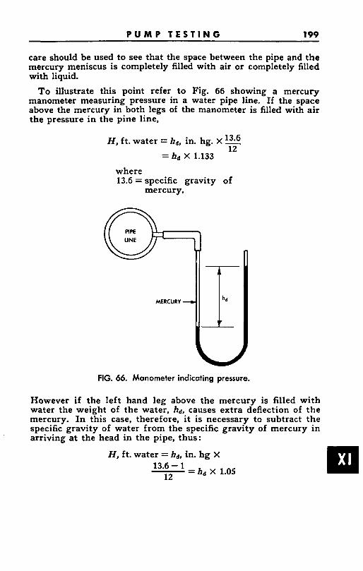
P U M P T E S T I N G 199
care should be used to see that the space between the pipe and the mercury meniscus is completely filled with air or completely filled with liquid.
To illustrate this point refer to Fig. 66 showing a mercury manometer measuring pressure in a water pipe line. If the space above the mercury in both legs of the manometer is filled with air the pressure in the pine line,
H, ft . water = hd, in. hg. X 13.6 - 12
= h d x 1.133
where 13.6 = specific gravity of
mercury.
FIG. 66. Manometer indicating pressure.
However if the left hand leg above the mercury is filled with water the weight of the water, h d , causes extra deflection of the mercury. I n this case, therefore, it is necessary to subtract the specific gravity of water from the specific gravity of mercury in arriving a t the head in the pipe, thus:
H, ft. water = hd, in. hg X 13.6 - 1
12 -=hb X 1.05
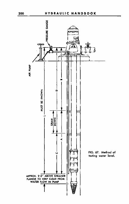
200 H Y D R A U L I C H A N D B O O K
FIG. 67. Method of testing water level.
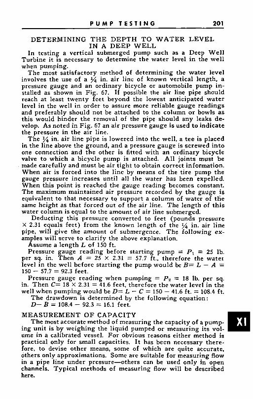
P U M P T E S T I N G 20 1
DETERMINING T H E D E P T H T O W A T E R LEVEL I N A D E E P WELL
In testing a vertical submerged pump such as a Deep Well Turbine i t is necessary to determine the water level in the well when pumping.
The most satisfactory method of determining the water level involves the use of a M in. air line of known vertical length, a pressure gauge and an ordinary bicycle or automobile pump in- stalled as shown in Fig. 67. If possible the air line pipe should reach at least twenty feet beyond the lowest anticipated water level in the well in order to assure more reliable gauge readings and preferably should not be attached to the column or bowls as this would hinder the removal of the pipe should any leaks de- velop. As noted in Fig. 67 an air pressure gauge is used t o indicate the pressure in the air line.
The M in. air line pipe is lowered into the well, a tee is placed in the line above the ground, and a pressure gauge is screwed into one connection and the other is fitted with an ordinary bicycle valve to which a bicycle pump is attached. All joints must be made carefully and must be air tight to obtain correct information. When air is forced into the line by means of the tire pump the gauge pressure increases until all the water has been expelled. When this point is reached the gauge reading becomes constant. The maximum maintained air pressure recorded by the gauge is equivalent to that necessary to support a column of water of the same height as that forced out of the air line. The length of this water column is equal to the amount of air line submerged.
Deducting this pressure converted to feet (pounds pressure X 2.31 equals feet) from the known length of the % in. air line pipe, will give the amount of submergence. The following ex- amples will serve to clarify the above explanation.
Assume a length L of 150 f t . Pressure gauge reading before starting pump = P I = 25 lb.
per sq. in. Then A = 25 X 2.31 = 57.7 ft., therefore the water level in the well before starting the pump would be B= L - A = 150 - 57.7 = 92.3 feet.
Pressure gauge reading when pumping = Pz = 18 lb. per sq. in. Then C= 18 X 2.31 = 41.6 feet, therefore the water level in the well when pumping would be D= L - C = 150 - 41.6 f t . = 108.4 ft.
The drawdown is determined by the following equation: D- B = 108.4 - 92.3 = 16.1 feet.
MEASUREMENT OF CAPACITY The most accurate method of measuring the capacity of a pump-
ing unit is by weighing the liquid pumped or measuring its vol- ume in a calibrated vessel. For obvious reasons either method is practical only for small capacities. It has been necessary there- fore, to devise other means, some of which are quite accurate, others only approximations. Some are suitable for measuring flow in a pipe line under pressure-others can be used only in open channels. Typical methods of measuring flow will be described here.
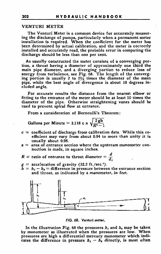
202 H Y D R A U L I C H A N D B O O K
VENTURI METER
The Venturi Meter is a common device for accurately measur- ing the discharge of pumps, particularly when a permanent meter installation is required. When the coefficient for the meter has been determined by actual calibration, and the meter i s correctly installed and accurately read, the probable error in computing the discharge should be less than one per cent.
As usually constructed the meter consists of a converging por- tion, a throat having a diameter of approximately one third the main pipe diameter, and a diverging portion to reduce loss of energy from turbulence, see Fig. 68. The length of the converg- ing portion is usually 2 to 2% times the diameter of the main pipe, while the best angle of divergence is about 10 degrees in- cluded angle.
For accurate results the distance from the nearest elbow or fitting to the entrance of the meter should be at least 10 times the diameter of the pipe. Otherwise straightening vanes should be used to prevent spiral flow at entrance.
From a consideration of Bernoulli’s Theorem :
Gallons per Minute = 3.118 c a dzl c = coefficient of discharge from calibration data. While this co-
efficient may vary from about 0.94 to more than unity i t is usually about 0.98.
a = area of entrance section where the upstream manometer con- nection is made, in square inches.
d R = ratio of entrance to throat diameter = - di
g = acceleration of gravity (32.2 ft./sec.*). h = hl - h, = difference in pressure between the entrance section
and throat, as indicated by a manometer, in feet.
FIG. 68. Venturi meter.
In the illustration Fig. 68 the pressures hl and h, may be taken by manometer as illustrated when the pressures are low. When pressures are high a differential mercury manometer which indi- cates the difference in pressure h, - h, directly, is most often
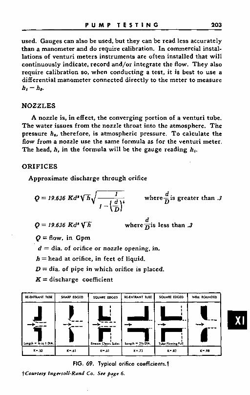
P U M P T E S T I N G 203
used. Gauges can also be used, but they can be read less accurately than a manometer and do require calibration. In commercial instal- lations of venturi meters instruments are often installed that will continuously indicate, record and/or integrate the flow. They also require calibration so, when conducting a test, it is best to use a differential manometer connected directly to the meter to measure hi - h,.
NOZZLES
A nozzle is, in effect, the converging portion of a venturi tube. The water issues from the nozzle throat into the atmosphere. The pressure h,, therefore, is atmospheric pressure. To calculate the flow from a nozzle use the same formula as for the venturi meter. The head, h, in the formula will be the gauge reading hl.
ORIFICES
Approximate discharge through orifice
d where-is greater than .3 1
Q = 19.636 K d ' f l d D 1 - ($1'
d Q = 19.636 K d L u
Q=flow, in Gpm d = dia. of orifice or nozzle opening, in.
h = head at orifice, in feet of liquid.
D = dia. of pipe in which orifice is placed.
K = discharge coefficient
whereBis less than .3
c RE-ENTW T U I SUARP EDGED SQU*RE EDGED RE.ENTRANT TUBE SQUARE EDGED WELL ROUNDED
l(=.52 K=.61 K==.61 K-.73 K=.8? KP.98
FIG. 69. -Typical orifice c0efficients.t
$Courtesy Ingersoll-Rand Co. See page 6.
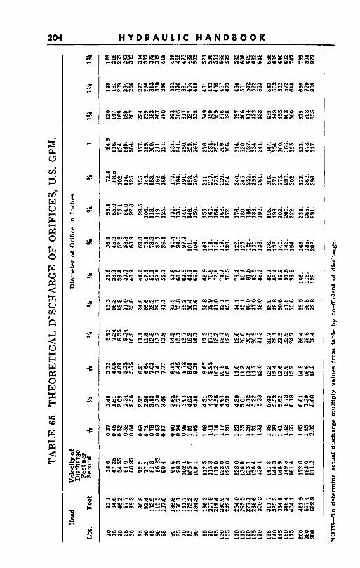
204 H Y D R A U L I C H A N D B O O K
c
c
f;
B ;
d
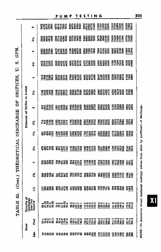
P U M P T E S T I N G 205
W
s n
n
2 d
rc
s n
n
.* n- N
s N
s N
N
.* el- .+
s r(
0
k c
c m
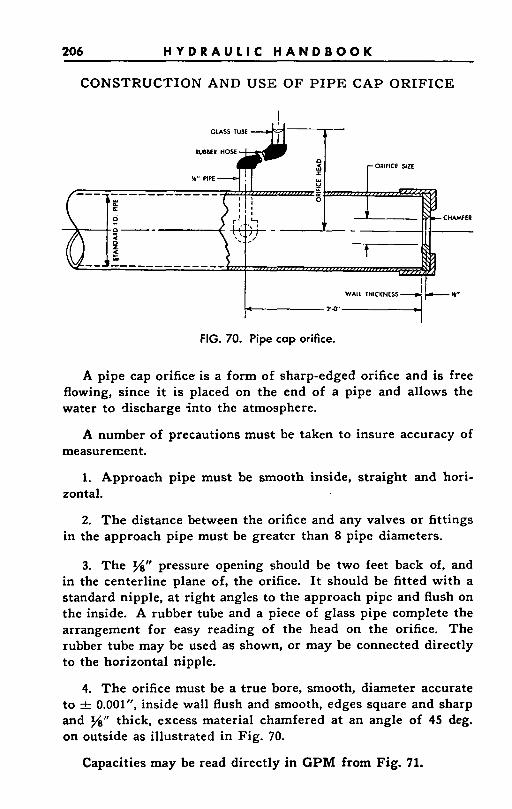
206 H Y D R A U L I C H A N D B O O K
CONSTRUCTION AND USE OF PIPE CAP ORIFICE
FIG. 70. Pipe cap orifice.
A pipe cap orifice is a form of sharp-edged orifice and is free flowing, since it is placed on the end of a pipe and allows the water to discharge into the atmosphere.
A number of precautions must be taken to insure accuracy of measurer-ent.
1. Approach pipe must be smooth inside, straight and hori- zontal.
2. The distance between the orifice and any valves or fittings in the approach pipe must be greater than 8 pipe diameters.
3. The S'' pressure opening should be two feet back of, and in the centerline plane of, the orifice. It should be fitted with a standard nipple, at right angles to the approach pipe and flush on the inside. A rubber tube and a piece of glass pipe complete the arrangement for easy reading of the head on the orifice. The rubber tube may be used as shown, or may be connected directly to the horizontal nipple.
4. The orifice must be a true bore, smooth, diameter accurate to & 0.001". inside wall flush and smooth, edges square and sharp and %'' thick, excess material chamfered a t an angle of 45 deg. on outside as illustrated in Fig. 70.
Capacities may be read directly in GPM from Fig. 71.
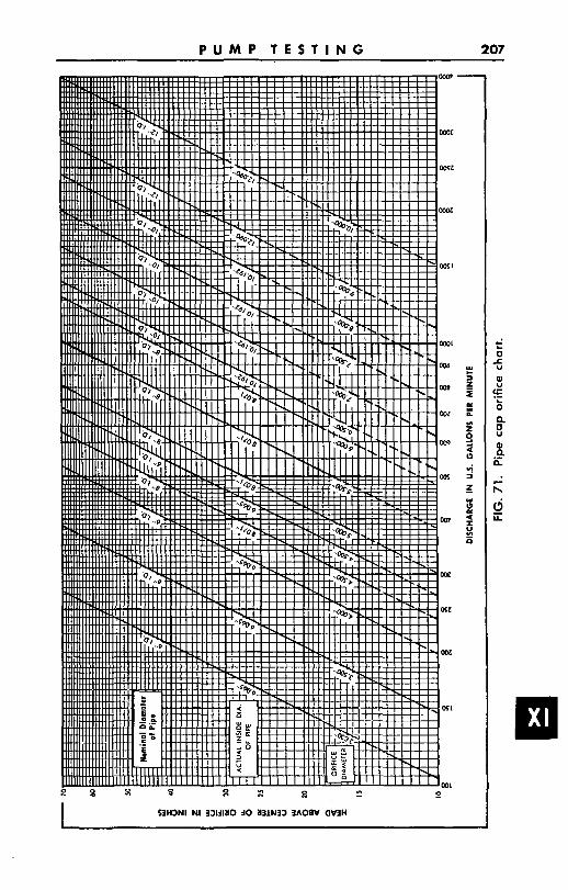
P U M P T E S T I N G 207
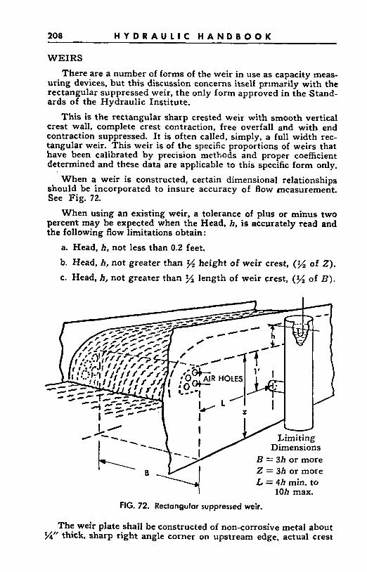
208 H Y D R A U L I C H A N D B O O K
WEIRS
There are a number of forms of the weir in use as capacity meas- uring devices, but this discussion concerns itself primarily with the rectangular suppressed weir, the only form approved in the Stand- ards of the Hydraulic Institute.
This is the rectangular sharp crested weir with smooth vertical crest wall, complete crest contraction, free overfall and with end contraction suppressed. I t is often called, simply, a full width rec- tangular weir. This weir is of the specific proportions of weirs that have been calibrated by precision methods and proper coefficient determined and these data are applicable to this specific form only.
When a weir is constructed, certain dimensional relationships should be incorporated to insure accuracy of flow measurement. See Fig. 72.
When using an existing weir, a tolerance of plus or minus two percent may be expected when the Head, h, is accurately read and the following flow limitations obtain :
a. Head, h, not less than 0.2 feet,
b. Head, h, not greater than % height of weir crest, (% of 2). c. Head, h, not greater than ‘/z length of weir crest, (% of B).
/ I- I -
Limiting Dimensions
B =I 3h or more Z = 3h or more L = 4h min. to
- 1 10h max. FIG. 72. Rectangular suppressed weir.
The weir plate shall be constructed of non-corrosive metal about %” thick, sharp right angle corner on upstream edge, actual crest
P U M P T E S T I N G 209
width %”, with plate beveled at 45O angle from crest on the down- stream face. The crest shall be. smooth and free from rust, grease, algae, etc., during testing. The plate must be mounted in a vertical plane at right angles to the line of flow, with the crest absolutely level. The channel walls shall be smooth and parallel and shall extend downstream beyond the overfall, and above the crest level. Complete aeration of the nappe is required, and observations before and during test are necessary to provide evidence of complete free- dom from adhering nappe, disturbed or turbulent flow, or surging. The weir shall be located sufficiently downstream from the source to insure that smooth flow, free from eddies, surface disturbance, or excessive air in suspension, is maintained at all flow rates. Since slight deviation from proper conditions can cause appreciable varia- tion in the indicated quantity, proper baffling is very important in order to give approximately uniform velocity across the approach channel. This channel must be of uniform cross section, straight and free from stilling racks or other obstructions for a length equal to at least fifteen times the maximum head on the weir. If out of doors, protection should be provided against surface disturbance from wind.
The head on the weir shall be measured by hook gages, securely placed in stilling boxes located at the side of the approach channel, upstream from the crest a distance, L, of between four and ten times the maximum head, h, on the weir. The stilling boxes shall com- municate with the channel by a pipe about 1%” in diameter, flush with the side of the channel and approximately one foot below the level of the crest. If located out of doors, protection against wind pressure and entrance of foreign material shall be provided.
Table 66 gives the flow over this type of weir, based on the Francis formula, Q = 3.33BhS/’, where Q = flow in cu. ft./second, B = crest length in feet, and h = head on the weir in feet. While this is an approximation, it is a close one, and is accurate enough for many field tests.
However, where accurate field testing is desired and precise in- struments are available to measure the head, h, the Rehbock formula should be used as follows :
Q = (3.228 + 0.435&)Bhe3/a 2
where : Q = quantity in Cu. ft./sec. he = h + 0.0036 h = observed head on crest, in feet, without correction for
z = height of weir crest above bottom of channel of approach,
B = length of weir crest, in feet.
velocity of approach.
in feet.

210 H Y D R A U L I C H A N D B O O K
TABLE 66. FLOW OVER RECTANGULAR SUPPRESSED WEIR IN CU. FT. PER SECOND. Q=3.33BhJIa
Crest Length in Feet
Head Ft. 1.0 1.5 2.0 3.0 4 .O 5.0 6.0 7.0 8.0
0.1 0.2 0.3 0.4 0.5 0.6 0.7 0.8 0.9 1.0 1.1 1.2 1.3 1.4 1.5 1.6
1.7 1.8 1.9 2.0 2.1 2.2 2.3 2.4 2.5 2.6 2.7 2.8 2.9 3.0
0.11 0.30 0.65 0.84 1.18 1.55 1.95 2.38 2.84 3.33 3.84
4.38 4.94 5.52 6.12 6.74 7.38 8.04 8.72 9.42 10.13 10.87 11.62 12.38 13.16 13.96 14.77 15.60 16.45 17.30
0.16 0.45 0.82 1.26 1.77 2.32 2.93 3.57 4.26 5.00 5.76 6.57 7.40 8.27 9.18 10.11
11.08 12.06 13.08 14.13 15.20 16.30 17.42 18.57 19.74 20.94 22.16 23.40 24.67 25.95
0.21
0.60 1.09 1.68 2.35 3.10 3.90 4.77 5.69 6.66
7.68
8.75 9.87 11.03 12.24 13.48
14.76 16.08 17.44 18.84 20.27 21.73 23.23 24.76 26.33 27.92 29.55 31.20 32.89 34.61
0.32 0.89 1.64 2.53 3.53 4.64 5.85 7.15 8.53 9.99 11.53
13.13 14.81 16.55 18.35 20.22
22.14 24.13
26.16 28.26 30.40 32.60 34.85 37.14 39.49 41.88 44.32 46.81 49.34 51.91
0.42
1.19 2.19 3.37 4.71 6.19 7.80 9.53 11.37 13.32
15.37 17.51 19.74 22.06 24.47 26.96
29.52 32.17 34.89 37.68 40.54 43.46 46.46 49.52 52.65 55.84 59.10 62.41 65.78 69.21
0.53 1.49 2.74 4.21 5.89 7.74 9.75 11.91 14.22 16.65 19.21
21.89 24.68 27.58 30.59 33.70
36.91 40.21 43.61 47.10 50.67 54.33 58.08 61.91 65.82 69.81 73.87 78.01 82.23 86.52
0.63 1.79 3.28 5.05 7.06 9.29 11.70 14.30 17.06 19.98 23.05 26.26 29.61 33.10 36.71 40.44
44.29 48.25 52.33 56.51 60.80 65.20 69.69 74.29 78.98 83.77 88.64 93.61 98.67 103.82
0.74 2.08 3.83 5.90 8.24 10.83 13.65 16.68 19.90 23.31 26.89
30.64 34.55 38.61 42.82 47.18
51.67 56.29 61.05 65.93 70.94 76.06 81.31 86.67 92.14 97.73 103.42 109.21 115.12 121.12
0.84 2.38 4.38 6.74 9.42
12.38 15.60 19.06 22.76 26.64 30.73
35.02 39.49 44.13 48.94 53.92 59.05 64.33 69.77 75.35 81.07 86.93 92.92 99.05 105.30 111.69 118.19 124.82 131.56 138.42
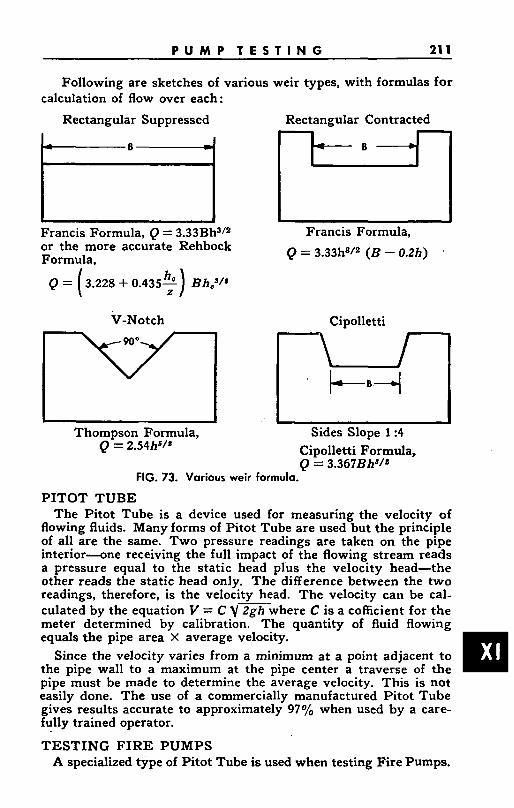
P U M P T E S T I N G 21 1
Following are sketches of various weir types, with formulas for calculation of flow over each:
Rectangular Suppressed
E Francis Formula, Q = 3.33Bh3I2 or the more accurate Rehbock Formula,
Q = (3.228 + V-Notch
Rectangular Contracted
Francis Formula, Q = 3.33h812 (B - 0.2h)
Cipolletti
Thompson Formula, Q = 2.54h61s
Sides Slope 1 :4 Cipolletti Formula, Q = 3.367Bhs/S
FIG. 73. Various weir formula.
PITOT TUBE The Pitot Tube is a device used for measuring the velocity of
flowing fluids. Many forms of Pitot Tube are used but the principle of all are the same. Two pressure readings are taken on the pipe interior-one receiving the full impact of the flowing stream reads a pressure equal to the static head plus the velocity head-the other reads the static head only. The difference between the two readings, therefore, is the velocity head. The velocity can be cal- culated by the equation V = C V 2gh where C is a cofficient for the meter determined by calibration. The quantity of fluid flowing equals the pipe area x average velocity.
Since the velocity varies from a minimum a t a point adjacent to the pipe wall to a maximum at the pipe center a traverse of the pipe must be made to determine the average velocity. This is not easily done. The use of a commercially manufactured Pitot Tube gives results accurate to approximately 97% when used by a care- fully trained operator.
TESTING F I R E PUMPS A specialized type of Pitot Tube is used when testing Fire Pumps.
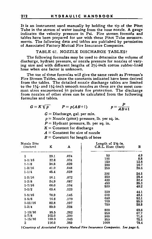
21 2 H Y D R A U L I C H A N D B O O K
(inches) K A -- -
I t is an instrument used manually by holding the tip of the Pitot Tube in the stream of water issuing from the hose nozzle. A gauge indicates the velocity pressure in Psi. Fire stream formula and tables have been prepared for use with these Pitot Tube measure- ments. The following data and tables are published by permission of Associated Factory Mutual Fire Insurance Companies.
TABLE 67. NOZZLE DISCHARGE TABLESt The following formulas may be used to determine the volume of
discharge, hydrant pressure, or nozzle pressure for nozzles of vary- ing size and with different lengths of Zs-inch cotton rubber-lined hose when one factor is unknown.
The.use of these formulas will give the same result as Freeman's Fire Stream Tables, since the constants indicated have been derived from the tables. The detailed nozzle discharge tables are limited to the 1%- and l%-inch smooth nozzles as these are the most com- mon sizes encountered in private fire protection. The discharge from nozzles of other sizes can be calculated from the following formulas and tables.
C.R.L. Hose (feet) B
G = K ~ P = p(AB+l) P p = m
1 1-1/16 1-118 1-3/16 1-114 1-5!16 1-318 1-7/16 1-112
1-9/16 1-518 1-11/16 1-314 1-13/16 1-718 1-15/16 2
29.1 32.8 36.8 41.0 45.4 50.1 54.9 60.0 65.4
70.9 76.8 82.8 89.0 95.5 102.0 109.0 116.0
.024
.031
.039
.048
.059
.072
.087
.lo4
.123
.145
.170
.197
.228
.262
.300
.343
.389
50 100 150 200 250 300 350 400 450 500
550 GOO 650 700 750 800 850 900 950 1000
4.9 8.8 12.8 16.7 20.6 24.5 28.4 32.4 35.3 40.2 44.1 48.1 62.1 65.9 58.8 63.8 67.7 71.6 75.5 79.4
t Courtesy of Associated Factory Mutual Fire Insurance Companies. See page 6.
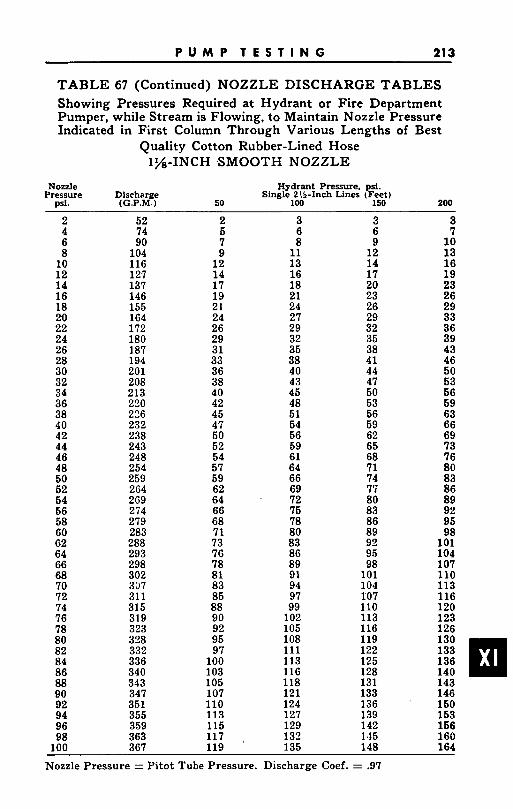
P U M P T E S T I N G 21 3
TABLE 67 (Continued) NOZZLE DISCHARGE TABLES Showing Pressures Required at Hydrant or Fire Department Pumper, while Stream is Flowing, to Maintain Nozzle Pressure Indicated in First Column Through Various Lengths of Best
Quality Cotton Rubber-Lined Hose lf/B-INCH SMOOTH NOZZLE
N o d e Hydrant Pressure, psi. Pressure Discharge Single Z!i-Inch Lines (Feet)
Psf. (G.P.M.) 50 100 150 200
2 52 4 74 6 90 8 104 10 12 14
iiS 127 137
16 146 18 155 20 164 22 172 24 180 26 187 28 194 ~~ ~ ~- 30 201 32 208 34 213 36 220 38 226 ._
40 232 42 238 44 243 46 248 48 254 50 259 52 264 54 2G9 56 274 58 279 60 283 62 288 64 293 66 298 68 302 70 307 72 311 74 315 76 319 78 323 80 328 82 332 84 336 86 340 88 343 90 347 92 351 94 355 96 359
2 5 7 9 12 14 17 19 21 24 26 29 31 33 36 38 40 42 45 47 50 52 54 57 59 62 64 66 68 71 73 76 78 81 83 85 88 90 92 95 97 100 103 105 107 110 113 115
3 6 8 11 13 16 18 21 24 27 29 32 35 38 40 43 45 48 51 54 56 59 61 64 66 69 72 75 78 80 83 86 89 91 94 97 99 102 105 108 111 113 116 118 121 124 127 129
3 6 9 12 14 17 20 23 26 29 32 35 38 41 44 47 50 53 56 59 62 65 68 71 74 77 80 83 86 89 92 95 98 101 104 107 110 113 116 119 122 125 128 131 133 136 139 142
3 7 10 13 16 19 23 26 29 33 36 39 43 46 50 63 56 69 63 66 69 73 76 80 83 86 89 92 95 98 101 104 107 110 113 116 120 123 126
146 150 163 166 _ _
98 363 ii7 , 132 I .I5 160 100 367 119 135 148 164
Nozzle Pressure = Pitot Tube Pressure. Discharge Coef. = .97
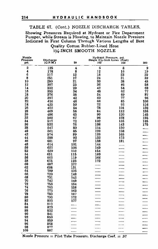
214 H Y D R A U L I C H A N D B O O K
TABLE 67. (Cont.) NOZZLE DISCHARGE TABLES. Showing Pressures Required at Hydrant or Fire Department Pumper, while Stream is Flowing, to Maintain Nozzle Pressure Indicated in First Column Through Various Lengths of Best
Quality Cotton Rubber-Lined Hose l%-INCH SMOOTH NOZZLE
Nozzle H drant Pressure. psi. Pressure Discharge slngre 2 !$-Inch Lines (Feet)
psi. (G.P.M.) 50 100 150 200
2 . 125 4 178 6 217 8 251 10 280 12 307 14 332 16 355 18 376 20 397 22 416 24 435 26 452 28 469 30 486 32 502 34 517 36 538 38 547 40 561 42 574 44 588 46 601 ~. - _ _ 48 614 50 627 52 639 54 651 66 663 58 675 60 687 62 698 64 709 ~~ ... 66. 720 68 73 1 70 742 72 753 74 763 . - . _ _ 76 773 78 783 80 793 82 803 .~ -.-
84 813 86 823 88 832 90 841 92 850 94 859 96 868 98 877 100 887
4 8 13 17 21 25 29 34 38 42 46 50 54 68 63 67 72 76 80 85 89 93 97 101 106 110 115 119 123 127 131 135 140 145 149 154 158 163 167 172 177 ......
6 8 12 16 18 23 24 31 _ _ ~~
30 38 36 46 42 54 48 62 54 69 60 77 66 85 72 93 78 101 . - - . ~
84 112 90 120 96 128 102 135 108 114 120
143 150 158
126 165 132 173 138 181 144 ...... 149 ...... 160 166 172
__._.. ...... ......
._..__ ......
...... _._.__ ...... ._..__ ......
._..__ ......
...... ......
...... ......
.._.__ ......
...... ......
...... ......
9 19 29 39 48 58 68 77 87 96 106 116 126 135 145 155 165 175 ...... .---.. ..--_. ...... ...... _____.
.__._.
.---.-
.__._.
......
......
......
...... I..._
Nozzle Pressure = Pilot Tube Pressure. Discharge Coef. = .97
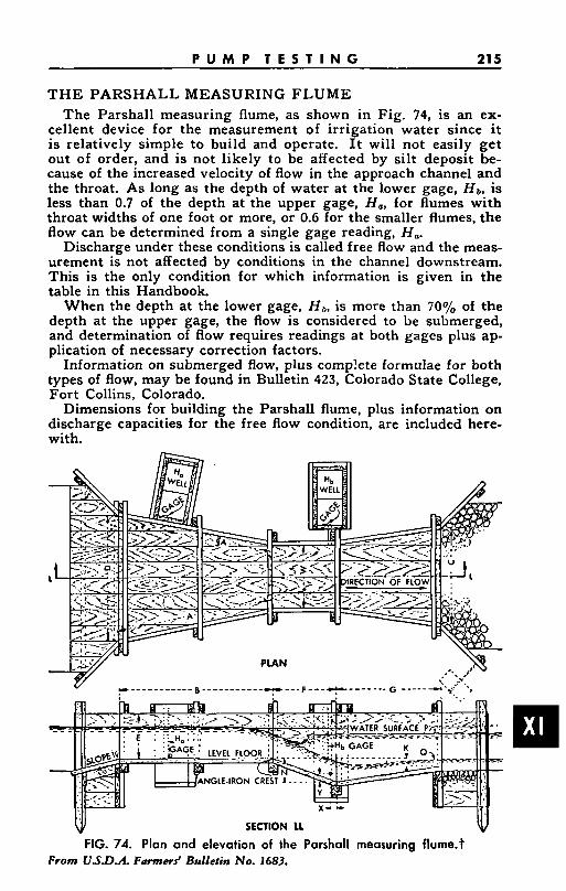
P U M P T E S T I N G 21 5
T H E PARSHALL MEASURING FLUME The Parshall measuring flume, as shown in Fig. 74, is an ex-
cellent device for the measurement of irrigation water since it is relatively simple to build and operate. I t will not easily get out of order, and is not likely to be affected by silt deposit be- cause of the increased velocity of flow in the approach channel and the throat. As long as the depth of water a t the lower gage, Ha, is less than 0.7 of the depth at the upper gage, H a , for flumes with throat widths of one foot or more, or 0.6 for the smaller flumes, the flow can be determined from a single gage reading, Ha.
Discharge under these conditions is called free flow and the meas- urement is not affected by conditions in the channel downstream. This is the only condition for which information is given in the table in this Handbook.
When the depth at the lower gage, H b , is more than 70% of the depth at the upper gage, the flow is considered to be submerged, and determination of flow requires readings at both gages plus ap- plication of necessary correction factors.
Information on submerged flow, plus comp!ete formulae for both types of flow, may be found in Bulletin 423, Colorado State College, Fort Collins, Colorado.
Dimensions for building the Parshall flume, plus information on discharge capacities for the free flow condition, are included here- with.
. . .
SECTION 11
FIG. 74. Plan and elevation of the Parshall measuring f1ume.t From U.S.D.A. Fawners' Bulleiin No. 1683.
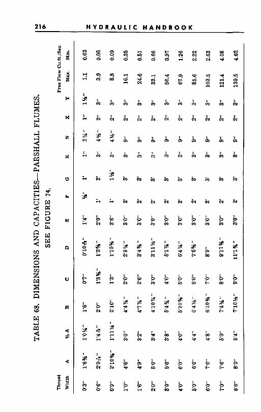
216 H Y D R A U L I C H A N D B O O K
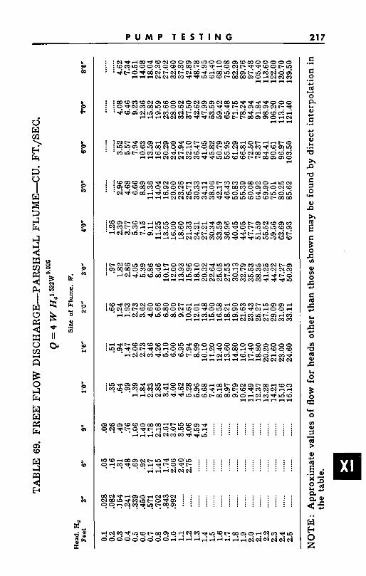
P U M P T E S T I N G 217
E .I
E 0
m 0
0
E
.d c,
c(
Ef. c,
.I
c. 0 Q) l.4
U x P U E
.d
w Q)
x : E 0 4
5
5
5
2 2
Q) m 0
E m
l.4 0)
0 m
l.4
w 0
3 0 G
0 Iu
.. w w 0 z
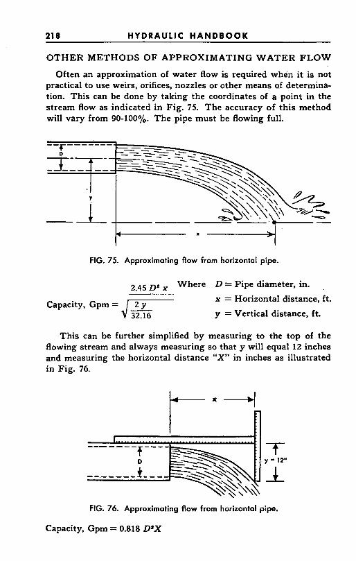
21 8 HYDRAULIC H A N D B O O K
OTHER METHODS O F APPROXIMATING WATER FLOW
Often an approximation of water flow is required when it is not practical to use weirs, orifices, nozzles or other means of determina- tion. This can be done by taking the coordinates of a point in the stream flow as indicated in Fig. 75. The accuracy of this method will vary from 90-100~o. The pipe must be flowing full.
FIG. 75. Approximating flow from horizontal pipe.
2.45 Ds Where D = Pipe diameter, in. x = Horizontal distance, ft.
y = Vertical distance, ft. Capacity, Gpm =
This can be further simplified by measuring to the top of the flowing stream and always measuring so that y will equal 12 inches and measuring the horizontal distance “X” in inches as illustrated in Fig. 76.
FIG. 76. Approximating flow from horizontal pipe.
Capacity, Gpm = 0.818 P X
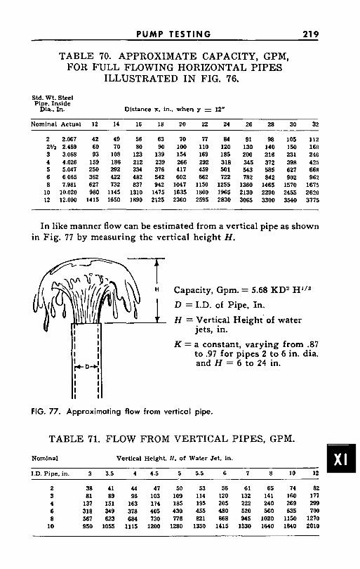
PUMP T E S T I N G 21 9
TABLE 70. APPROXIMATE CAPACITY, GPM, FOR FULL FLOWING HORIZONTAL PIPES
ILLUSTRATED IN FIG. 76.
Std. Wt. Steel Pipe, Inside
Dia.. In. Distance x. in., when y = 12"
Nominal Actual 12 14
2 2.067 2% 2.469 3 3.068 4 4.026 5 5.047 6 6.065 8 7.981
10 10.020 12 12.000
42 60 93
159 250 362 627 980
1415
49 70
108 186 292 422 732
1145 1650
16
56 80
123 212 334 482 837
1310 1890
- 18 20
63 90
139 239 376 542 942
1475 2125
70 100 154 266 417 602
1047 1635 2360
22
77 110 169 292 459 662
1150 1800 2595
- 24
84 120 185 318 501 722
1255 1965 2830
- 26
9 1 130 200 345 543 782
1360 2130 3065
- 28
98 140 216 372 585 842
1465 2290 3300
~
30
105 150 231 398 627 902
1570 2455 3540
32
112
246 425 668 962
1675 2620 3775
-
160
In like manner flow can be estimated from a vertical pipe as shown in Fig. 77 by measuring the vertical height H.
Capacity, Gpm. = 5.68 KDz
D = I.D. of Pipe, In. H = Vertical Height of water
jets, in. K = a constant, varying from .87
to .97 for pipes 2 to 6 in. dia. and H = 6 to 24 in.
FIG. 77. Approximating flow from vertical pipe.
TABLE 71. FLOW FROM VERTICAL PIPES. GPM.
Nominal Vertical Height. H. of Water Jet. in.
1.D.Pipe. in. 3 3.5 4 4.5 5 5.5 6 7 8 10 12
2 38 41 44 47 50 53 56 6 1 65 74 82 3 81 89 96 103 109 114 120 132 141 160 177 4 137 151 163 174 185 195 205 222 240 269 299 6 318 349 378 405 430 455 480 520 560 635 700 8 567 623 684 730 776 821 868 945 1020 1150 1270
10 950 1055 1115 1200 1280 1350 1415 1530 1640 1840 2010
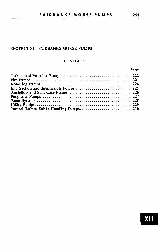
F A I R B A N K S M O R S E P U M P S 22 1
SECTION XI1 . FAIRBANKS MORSE PUMPS
CONTENTS
Page 'hrbine and Propeller Pumps .................................... 222 Fire Pumps .................................................... 223 Non-Clog Pumps ............................................... 2~ End Suction and Submersible Pumps ............................. 225 Angleflow and Split Case Pumps ................................. 226 Peripheral Pumps .............................................. 227 Water Systems ................................................. 228 Utility Pumps .................................................. 229 Vertical 'kbine Solids Handling Pumps ............................ 230
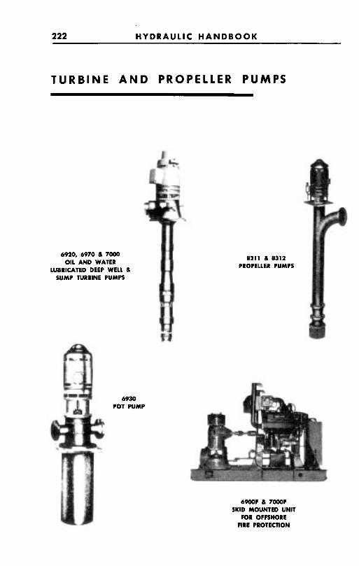
222 HYDRAULIC HANDBOOK
T U R B I N E A N D P R O P E L L E R P U M P S
6920, 6970 6 7000 OIL A N D WATER
LUBRICATED DEEP WELL 6 SUMP TURBINE PUMPS
6930 POT PUMP
8211 6 8312 PROPELLER PUMPS
6900F 6 7000F SKID MOUNTED UNIT
FOR OFFSHORE ARE P R O T K n O N
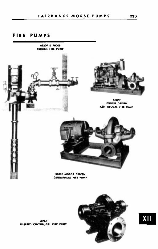
F A I R B A N K S M O R S E P U M P S 223
6920F 6 TOOOF TURBINE FIRE PUMP
HOOF ENGINE DRIVEN
CENTRIFUGAL FIRE PUMP
5876F HI-SPEED CENTRIFUGAL FIRE PUMP
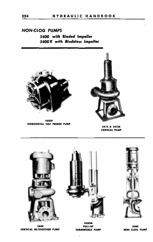
224 H Y D R A U L I C H A N D B O O K
NON-CLOG PUMPS 5400 with Bladed Impeller 5400 K with Bladeless Impeller
5420P HORIZONTAL SELF PRIMER PUMP
5 4 1 0 6 5410K VERllCAL PUMP
5430 VERTICAL BlLlOCETHER PUMP
54301 PULL-UP
SUBMERSIBLE PUMP 5440
MON CLOG PUMP
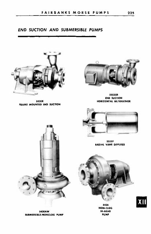
F A I R B A N K S M O R S E P U M P S 225
END SUCTION AND SUBMERSIBLE PUMPS
5520R FRAME MOUNTED END SUCTION
5430AW SUBMERSIBLE-NONCLOG PUMP
5553ER END SUCTION
HORIZONTAL BILTOGETHER
5553F RADIAL VANE DIFFUSER
5426 NON-CLOG
HI-HEAD PUMP

226 H Y D R A U L I C H A N D B O O K
ANGLEFLOW 8 SPUr CASE
5720 ANGLEFLOW
5800 SPUT CASE
5710 ANGLEFLOW
5740 ANGLEFLOW
5900 MULTISTAGE SPLIT CASE
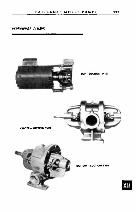
F A I R B A N K S M O R S E P U M P S 227
PERIPHERAL PUMPS
K)P-SUCTION TYPE
CENTER-SUCTION TYPE
BOTTOM-SUCTION TYPE
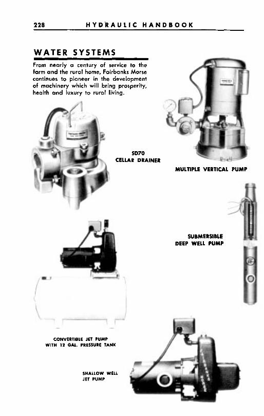
228 H Y D ' R A U L I C H A N D B O O K
WATER S Y S T E M S ~ ~~ ~~ ~
From nearly a century of service to the farm and the rural home, Fairbanks Morse continues to pioneer in the development of machinery which will bring prosperity, health and luxury to rural living.
SDIO CELLAR DRAINER
MULTIPLE VERTICAL PUMP
SUBMERSIBLE DEEP WELL PUMP
CONVERTIBLE JET PUMP WITH 12 GAL. PRESSURE TANK
SHALLOW WELL JET PUMP
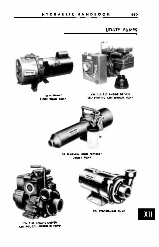
H Y D R A U L I C H A N D B O O K 229
UTILITY PUMPS
"Rain Maker" CENTRIFUGAL PUMP
ESP 315-320 ENGINE DRIVEN SELF-PRIMING CENTRIFUGAL PUMP
58 MAGNUM HIGH PRESSURE uniiw PUMP
CIJ CENNTRIFUGAL PUMP
1 'h C1 JE ENGINE DRIVEN CENTRIFUGAL FERTILIZER PUMP
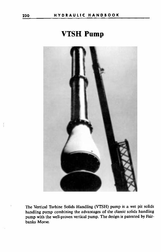
23 0 H Y D R A U L I C H A N D B O O K
VTSH Pump
The Vertical "brbine Solids Handling (VTSH) pump is a wet pit solids handling pump combining the advantages of the classic solids handling pump with the well-proven vertical pump. The design is patented by Fair- banks Morse.
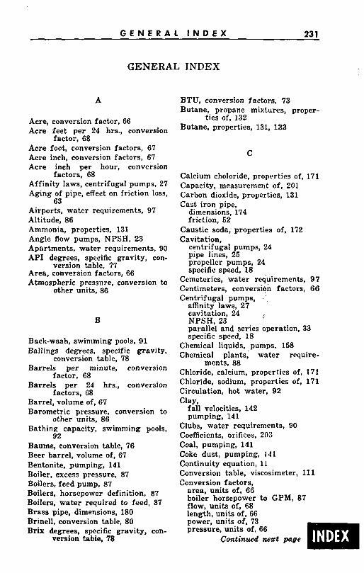
G E N E R A L I N D E X 23 1
GENERAL INDEX
A
Acre, conversion factor, 66 Acre feet per 24 hrs., conversion
Acre foot, conversion factors, 67 Acre inch, conversion factors, 67 Acre inch per hour, conversion
Affinity laws, centrifugal pumps. 27 Aging of pipe, effect on friction loss,
Airports, water requirements, 97 Altitude, 86 Ammonia, properties, 131 Angle flow pumps, NPSH, 23 Apartments, water requirements, 90 API degrees, specific gravity, con-
Area, conversion factors, 66 Atmospheric pressure, conversion to
other units, 86
factor, 68
factors, 68
63
version table, 77
B
Back-wash, swimming pools, 91 Ballings degrees, specific gravity,
Barrels per minute, conversion
Barrels pe r 24 hrs., conversion
Barrel, volume of, 67 Barometric pressure, conversion to
other units, 86 Bathing capacity, swimming pools,
92 Baume, conversion table, 76 Beer barrel, volume of, 67 Bentonite, pumping, 141 Boiler, excess pressure, 87 Boilers. feed pump, 87 Boilers, horsepower definition, 87 Boilers, water required to feed, 87 Brass pipe, dimensions, 180 Brinell, conversion table, 80 Brix degrees, specific gravity, con-
version table, 78
conversion table, 78
factor, 68
factors, 68
BTU, conversion factors, 73 Butane, propane mixtures, proper-
Butane, properties, 131, 133 ties of, 132
C
Calcium choloride, properties of, 171 Capacity, measurement of, 201 Carbon dioxide, properties, 131 Cast iron pipe,
dimensions, 174 friction, 52
Caustic soda, properties of, 172 Cavitation,
centrifugal pumps, 24 pipe lines, 25 propeller pumps, 24 specific speed, 18
Cemeteries, water requirements, 97 Centimeters, conversion factors, 66 Centrifugal pumps, ...
affinity laws, 27 cavitation, 24 NPSH, 23 parallel and series operation, 33 specific speed, 18
Chemical liquids, pumps, 158 Chemical plants, water require-
Chloride, calcium, properties of, 171 Chloride, sodium, properties of, 171 Circulation, hot water, 92
ments, 88
Clay, fall ve!ocities, 142 pumping, 141
Clubs, water requirements, 90 Coefficients, orifices, 203 Coal, pumping, 141 Coke dust, pumping, 141 Continuity equation, 11 Conversion table, viscosimeter, 111 Conversion factors,
area, units of, 66 boiler horsepower to GPM, 87 flow, units of, 68 leneth. units of. 66 power,. units of, 73 pressure, units of, 66
Continued next page
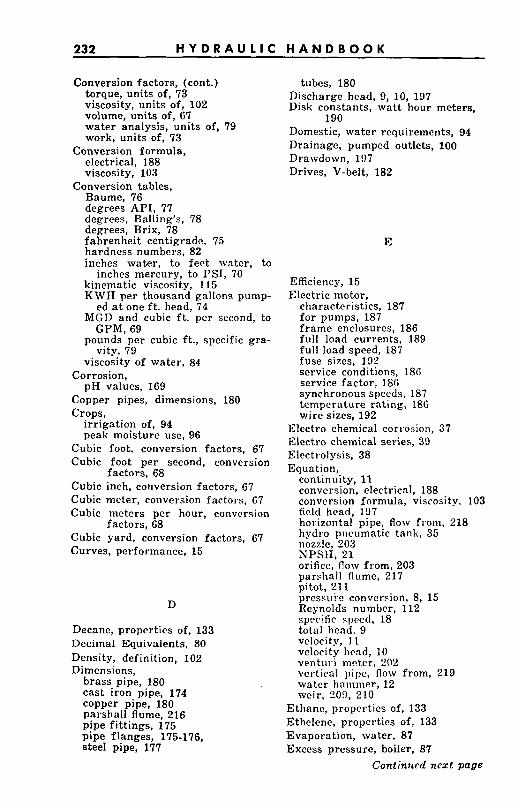
232 H Y D R A U L I C H A N D B O O K
Conversion factors, (cont.) torque, units of, 73 viscosity, units of, 102 volume, units of, 67 water analysis, units of, 79 work, units of, 73
Conversion formula, electrical, 188 viscosity, 103
Conversion tables, Baume, 76 degrees API, 77 degrees, Balling's, 78 degrees, Brix, 78 fahrenheit centigrade. 75 hardness numbers, 82 inches water, to feet water, to
inches mercury, to PSI, 70 kinematic viscosity, 115 KWH per thousand gallons pump-
ed at one f t . head. 74 M G D and -cubic ft . ' per second, to GPM, 69
pounds per cubic ft., specific gra-
viscosity of water, 84
p H values, 169
vity, 79
Corrosion,
Copper pipes, dimensions, 180 Crops,
irrigation of, 94 peak moisture use, 96
Cubic foot, conversion factors, 67 Cubic foot per second, conversion
Cubic inch, conversion factors, 67 Cubic meter, conversion factors, G7 Cubic meters per hour, convcrsion
factors, 68 Cubic yard, conversion factors, 67 Curves, performance, 15
factors, 68
D
Decane, propcrtics of, 133 Decimal Equivalents, 80 Density, definition, 102 Dimensions,
brass pipe, 180 cast iron pipe, 174 copper pipe, 180 parshall flume, 216 pipe fi t t ings, 175 pipe flanges, 175-176, steel pipe, 177
tubes, 180 Discharge head, 9, 10, 197 Disk constants, wat t hour meters,
Domestic, water requirements, 94 Drainage, pumped outlets, 100 Drawdown, 197 Drives, V-belt, 182
190
E
Efficiency, 15 Electric motor,
characteristics, 187 for pumps, 187 f rame enclosures, 186 full load currents, 189 full load speed, 187 fuse sizes, 332 service conditions, 18G service factor, 186 synchronous speeds, 187 tempcrature rating, 186 wire sizes, 192
Electro chemical corrosion, 37 Electro chemical series, 39 Electrolysis, 38 Equation,
continuity, 11 conversion, electrical, 188 Conversion formula, viscosity. 103 field head, 197 horizontal pipe, flow from, 218 hydro pnrumatic tank, 35 nozzle, 203 NPSH, 21 orifice, flow from, 203 parshall flume, 217 pitot, 211 presrui.e conversion, 8, 15 Reynolds number, 112 sprrific speed, 18 total hcnd. 9 velocity, I t velocity hcnd, 10 ventuyi meter, 202 vertical pipe, flow from, 219 water hammer, 12 weir, 209, 210
Ethane, propertics of, 133 Ethclene, propcrtics of, 133 Evaporation, water, 87 Excess pressure, boiler, 87
Continwd next page
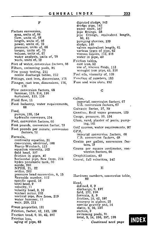
G E N E R A L I N D E X 233
F
Factors conversion, area, units of, 66 flow, units of, 68 length, units of, 66 power, units of, 73 pressure, units of, 66 torque, units of, 73 volume, units of, 67 water analysis, units of, 79 work, units of, 73
Feet of water, conversion factors, G6 Filters, swimming pools, 91 Fire pump testing, 211
Fittings, cast. iron, dimensions, 155 Flanges, cast iron, dimensions, 175,
Flow conversion factors, 68
nozzle discharge tables, 212
176
laminar, 113, 114, 116 turbulent, 113, 116
Fluid flow, 11 Food Industry, water requirements,
88 Food,
pumps, 138, 154 hydraulic conveyors, 154
Foot, conversion factors, 66 Foot pounds, conversion factor, 73 Foot pounds per minute, conversion
Formula, factors, 73
continuity equation, 11 conversion, electrical, 188 Darcy-Weisbach, 113 equation viscosity, 103 field head, 197 friction in pipes, 42 horizontal pipe, flow from, 218 hydro pneumatic tank, 3 G nozzle, 203 NPSH, 21, 22 orifice, 203 pressure head conversion, 8, 15 Reynolds number, 112 specific speed, 16 total head, 9 velocity, 11 velocity head, 9, 10 venturi meter, 202 vertical pipe, flow from, 219 water hammer, 11 weir, 209, 211
Freon properties, 131 Friction, factor, 42, 112, 120 Friction head, 9, 10, 42, 197 Friction loss,
aging of pipe, 63
digested sludge, 143 dredge pipe, 142 paper stock, 147 pipe fittings, 58 pipe fittings, equivalent length,
60, 61 pumping slurries, 139 sludge, 140 valves equivalent length, 61 various types of pipe, 62 viscous liquids, 112, 116 water in pipe, 42
Friction tables, cast iron, 52 use of, viscous fluids, 113 wrought iron pipe, 43, 116
Fuel oils, viscosity of, 109 Function of numbers, 183 Fuse and wire sizes, 192
G
Gallon, imperial, conversion factors, 67 U.S. conversion factors, 67 ,
Galvanic Series, 37, 39 Gasoline, Reid vapor pressure, 129 Gauge, pressure, 10, 194 Glass, sand, plaster of paris, pump-
Golf courses, water requirements, 97 GPM,
imperial conversion factors, G8 U.S. conversion factors, 68
Grains per gallon, conversion fac-
Grams per square centimeter, con-
Graphitization, 40 Gravel, fall velocities, 142
ing, 141
tors, 79
version factors, 66
H
Hardness numbers, conversion table,
Head, 82
defined, 8, 9 discharge, 9, 197 field, 197, 198 formula, 8, 9 friction, 10, 42, 197 recovery in siphon, 25 specific gravity and, 14 static, 9, 10, 197 suction. 9 swimming pools, 91 total, 9, 14, 196, 197, 198
Continued next page
234 H Y D R A U L I C H A N D B O O K
Head, (cont.) total, deep well pumps, 197 total dynamic, 9 velocity, formula, 9, 10, 197
Hectare, conversion factor, 66 Heptane, properties of, 133 Hexane, properties of, 133 Horizontal pipe, flow from, 218 Horsepower, 15, 16
boiler, definition, 87 conversion factors, 73 input to motor, 190
Horsepower hours, conversion fac- tors, 73
Horsepower metric, conversion fac- tors, 73
Hose; friction loss, 62 Hospitals, water requirements, 90 Hotels, water requirements, 90 Hydraulic Handbook, purpose, 8 Hydraulics, definition, 8 Hydrocarbon liquids, NPSH. 129, 130 vapor pressure, 130
Hydro-pneumatic tanks, 35
I Impeller,
peripheral velocity, 14 Inch, conversion factors, 66 Inches mercury, conversion factors,
Inches water, conversion factor, 66 Industrial plants, water require-
Irrigation,
66
ments, 88
frequency of, 96 overhead, water required, 97 quantity tables, 99 rates, various soils, 96 tables, 98
Irrigation, water requirements, 94 water requirements various cli-
water requirements various crops, mates, 96.
96 Iron dust, pumping, 141 Iron ore, pumping, 141 Iron pyrites, pumping, 141 Iso-butane, properties of, 133 Iso-pentane, properties of, 133
K Kilogram meters, conversion fac-
tors, 73
Kilograms per square cm. conversion
Kilometer, conversion factor, 66 Kilowatt, ' conversion factors, 73
Kilowatt hours,
factors, 66
input to motor, 16
conversion factors, 73 per thousand gallons, 16
L
Laminar flow, 113, 116 Length, conversion factors, 66 Liquids,
compressibility, 11 flow, 11 momentum, 11 viscous, 102 volatile, 128
Liter, conversion factor, 67 Liters per second, conversion factors,
68
M
Manometer, 198, 199 Materials of construction, pumps,
Mechanical seal, 161) Mercantile buildings, water require-
Meter,
158
ments, 90
conversion factors, 66 nozzle, 203 orifice, 203 parshall flume, 215 pipe cap orifice, 206 pitot tube, 211 venturi, 202 wat t hour, 190 weir, 208-211
imperial conversion factors, 68 U.S. conversion factors, 68
MCD,
Mile, conversion factors, 6G Milligrams per liter, conversion fac-
Millimeters mercury, conversion fac-
Miners inch, conversion factors, 68 Mixed flow pumps, NPSH, 23 Mixed flow pumps, specific speed, 18 Momentum, liquids, 11
Continued next page
tors, 79
tors, 66
G E N E R A L I N D E X 235
Motors, electric characteristics, 187 frame enclosures, 186 for pumps, 187 full load currents, 189 full load speed, 187 fuse sizes, 192 service conditions, 186 service factor, 186 synchronous speeds, 187 temperature rating, 186 wire sizes, 192
N Net positive suction head, 21
available, 21 definition, 21 hydro carbon liquids, 128, 129 required, 21 volatile liquids, 128, 129
Nonane, properties of, 133 Non-nietalic contruction material, 40 Nozzles, 203 Numbers,
functions of, 183
0 Octane, properties of, 133 Office buildings, water requirements,
Oil, barrel, volume of, 67 Oil, expansion-temperature, 136 Oil, petroleum, properties, 135 Orif ice,
90
capacity tables, 204 coefficients, 203 meter. 203 pipe cap orifice, construction of,
206
P Packing f o r various liquids, 161-167 Paper, manufacture of, 144 Paper and pulp industry, water re-
quirements, 88 Paper stock,
consistency, 144 consistency conversion, 152 conversion table, 152 definition, 144 friction i n pipe fi t t ings, 151 pumps, 138, 144
Parallel and series operation, cen-
Parshall flume, 215-217 tr ifugal pump, 33
Parts per million, conversion factors,
Pentane, properties of, 133 Performance curves, 15 Peripheral pumps, NPSH, 23 Petroleum industry, water require-
Petroleum oils, properties, 135 p H values, various liquids, 169
79
ments, 89
Pipe, cast iron. dimensions. 174 friction kbles , cast &on pipe, 52 friction tables, steel pipe, 43 friction of water in., 42 roughness, 42 roughness factors, 63
Pipe cap orifice, 206 Pipe fittings,
dimensions, 175 friction, paper stock, 151 friction loss, 58-61, 113, 114 resistance coefficient, 58, 59
Pipe flanges, dimensions, 175, 176 Pipe friction,
digested sludge, 143 dredge pipe, 142 fittings, paper stock, 151 paper stock, 147-150
slurries, 140 water, 43-57
pulp, 147-150
Pitot tube, fire pump testing, 211 Poise, 102 Positive displacement pumps, NPSH,
23 Pounds per cubic foot, specific gra-
vity conversion table, 79 Pounds per square inch, conversion
factors, 66 Power, conversion factors, 73 Pressure,
absolute, 8, 86 boiler excess, 87 conversion factor, 66 definition, 8 gauge, 10, 194 head, 8 measurement of, 194 vapor, water, 84
Products, Fairbanks-Morse, 222-228 Propane,
Butane, mixtures, properties of, 132
properties, 131, 133 Propeller pumps,
cavitation, 24 m Continued next page
236 H Y D R A U L I C H A N D B O O K
Propeller pumps, (cont.) NPSH, 23 specific speed, 17
Properties of gasoline, 134 Propylene, properties of, 133 Public buildings, water require-
ments, 90 Pulp,
conversion table, 152 definition, 144 friction in pipe fittings, 151 friction loss, 147-150
Pumping level in well, 197, 200 Pump Installation, food, 154-156 Pump,
bentonite, 141 bladeless, 139, 155 boiler feed, 87 centrifugal performance, 121 chemical liquids, 158 clay, 141 clogging, 138, 139 coal. 141 coke dust, 141 construction of, for abrasives,
drainage, 100 foods, 138,154, 155 foods, construction of, 154 glass, sand, plaster of paris, 141 hot water circulating, 92, 93 hydro carbon liquids, 129 irrigation, 94-100 iron dust, 141 iron ore, 141 iron pyrites, 141 materials recommended, 161-167 non clog, 138 paper stock, 144 paper stock selection, 144, 145, 146 performance, 198 reciprocating, viscous perf., 125 sand, 138, 139 sewage, 138, 139 sludge, 139, 140 slurries, 138, 139 storm water, 139 testing, 194 trash, 138 volatile liquid, 128 volatile liquid installation, 128
138,139
Q Quart , conversion, 67
R
Recirculation, swimming pools, 91 Reid, vapor pressure, 129
Relative roughness, definition, 112,
Residences, water requirements, 94 120
Resistance coefficient, pipe fittings, 58, 59
Reynolds number, 42, 112, 115, 120 Reynolds number equation, 112 Rockwell number, conversion table,
Rod, conversion factors, 66 Roughness factor, pipe, 63 Roughness, relative definition, 112 Rural, water requirements, 94
80
S
Sand, fall velocities, 142 Sand, pumps, 138 Saybolt Seconds Universal Viscosity,
103 Schools, water requirements, 90 Seal, mechanical, 168 Series and parallel operation, cen-
Sewage, tr ifugal pump, 33
pumps, 138, 139 pumps, bladeless, 139
Shore scleroscope number, conversion table, 80
Silt, fa l l velocities, 142 Siphons, 25 Sludge,
digested, 140 velocity in pipe lines, 140
Slugs, 102,112 Slurry, pumps, 138, 141 Soda, caustic, properties of, 172 Sodium chloride, properties of, 171 Soils,
DreciDitation rate. 96 wate; holding capacities, 95
Solids, in suspension, 138, 139 Specific gravity,
ammonia, 131 Baume, conversion factors, 76 butane, 131 carbon dioxide, 131 definition, 102 degrees API conversion table, 77 degrees Brix conversion table, 78 freon, 131 head, 14, 15 hydrocarbons, 130 hydrocarbon liquids, 130 pounds per cubic f t . conversion
table, 79 propane, 131
Continued next page
I N D E X OF T A B L E S 237
Specific gravity, (cont.) various liquids, 161-167 water, 84
Specific Speed, cavitation, 18 charts, 18, 20 definition, 16 formula, 18 pump proportions, 16, 17 suction limitation, 18, 20
Specific weight, water, 84 Static head,
defined, 9, 10 discharge, 9, 197, 199 suction, 10, 197, 198
Steel pipes, dimensions, 177-179 Stokes, 102 Storage capacity, .hydro pneumatic
tank, 35 Submergence, 197, 201 Suction Head, 10
net positive, 21 Suction, limitations specific speed, 18 Square centimeter, conversion factor,
Square foot, conversion factor, 66 Square inch, conversion factor, 66 Square kilometer, conversion factor,
Square meter, conversion factor, 66 Square mile, conversion factor, 66 Square yard, conversion factor, 66 Surge tanks, 11 Swimming pools,
66
66
back washing, 91 filter, 91 recirculation, 91 . total head, 91 water requirements, 91
Synthetic fuel, water requirements, 88
T
Tanks, capacity table, 181 hydro-pneumatic, 35 surge, 11
Testing pumps, 194 Textile industry, water requirements,
Torque, conversion factors, 73 Total head, 9
deep well pumps, 197-199 measurement of, 196
Turbulent flow, 112, 116 Tubes. dimension, 180
89
Turf, water requirements, 96
V
Valves, resistance coefficient, 58, 59 Vapor pressure,
ammonia, 131 butane, 131 butane, propane mixture, 132 carbon dioxide, 131 freon, 131 gasoline, 134 hydro carbons,130 hydro carbon liquids, 129 propane, 131 Reid, 129 water, 84
V-Belt, drives, 182 Velocity, 43, 52
abrasives, 139 clogging, 139 effect on corrosion, 37 fall, abrasives, 142 peripheral, 14
formula, 10 Velocity h&d, 10, 43, 52, 197
Velocity limit in siphon, 25 Venturi meter, 202 Vertical pipe, flow from, 219 Vickers pyramid conversion table, 80 Viscous liauids. 102
centrifugal pump performance,
reciprocating pump performance, 121-124
125 Viscosity,
absolute, 112 blending chart , 110 Conversion table, 111 definition, 102 dynamic, 102 fuel oils, 109 kinematic, 103, 112, 115 SSU, 103 temperature chart , 108 various liquids, 103-107
Volatile liquids, definition, 128 in storage, 128
Volume, conversion factors, 67
W Water,
boiling point of, 84, 86 flow measurement of, 201 hammer, 11 pound, conversion factor. 67
Continued next page
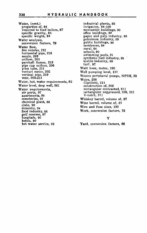
238 H Y D R A U L I C H A N D B O O K
Water, (cont.) properties of, 84 required to feed boilers, 87 specific gravity, 84 specific weight, 84
conversion factors, 79
fire nozzles, 212 horizontal pipe, 218 nozzle, 203 orifices, 203 parshall flumes, 216 pipe c a p orifices, 206 pitot tube, 211 venturi meter, 202 vertical pipe, 219 weir, 208-211
Water analysis,
Water flow,
Water, hot, water requirements, 92 Water level, deep well, 201 Water requirements,
a i r ports, 97 apartments, 90 cemeteries, 97 chemical plant, 88 clubs, 90 domestic, 94 food industry, 88 golf courses, 97 hospitals, 90 hotels, 90 hot water service, 92
industrial plants, 88 irrigation, 94-100 mercantile buildings, 90 office buildings, 90 paper and pulp industry, 88 petroleum industry, 89 public buildings, 90 residences, 94 rural , 94 schools, 90 swimming pools, 91 synthetic fuel industry, 89 . textile industry, 89 turf , 97
Wat t hour, meter, 190 Well pumping level, 197 Westco peripheral pumps, NPSH, 23 Weirs, 208
Cipolletti, 211 construction of, 208 rectangular contracted, 211 rectangular suppressed, 208, 211 V-notch, 211
Whiskey barrel, volume of, 67 Wine barrel, volume of, 67 Wire and fuse sizes, 192 Work, conversion factors, 73
Y
Yard, conversion factors, 66
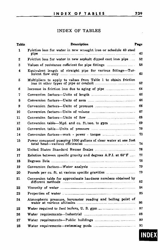
I N D E X O F T A B L E S 2 39
Table
1
2 3 4
5
6 7 8 9 10 11 12 13 14
15
16 17 18 19 20
21
22 23
24
25 26 27 28
INDEX OF TABLES
Description
Friction loss fGr water in new wrought iron o r schedule 40 steel
ter in new asphalt dipped cast iron pipe ......
Values of resistance cofficient for pipe fittings ...............................
Equivalent length of straight pipe fo r various fittings-Tur- bulent flow only ..................................................................................
Multipliers to apply to values from Table 1 to obtain fric loss in other types of pipe or conduit .....................................
Increase in friction loss due to aging of pipe ................................
Conversion factors-Units of length ...............................................
Conversion factors-Units of area ... ......................................... Conversion factors-Units of pressure ............................................ Conversion factors-Units of volume .. ....................... Conversion factors-Units of flow ....................................................
Conversion table-Mgd . and cu . ft./sec. to gpm ............................ Conversion table-units of pressure ......................
Conversion factors-work - power - torque ....................................
Power consumed pumping 1000 gallons of clear water at one foot total head-various efficiencies ........................................................
United States Standard Baume Scales .............
Relation between specific gravity and degrees A.P.I. at 60'F ......
...............................................................................
Degrees Brix ................................. ..........................................
Conversion factors-Water analysis .................................................
Pounds per cu . f t . at various specific gravities ...............................
Conversion table fo r approximate hardness numbers obtained by different methods . ................................................
Viscosity of water ..........._........................,............................................. Properties of water ................................... .............................
Atmospheric pressure, barom water at various altitudes .
Water required to feed boile
ding and boiling point of ...............................................
Water requirements-Industrial ............. .................
Water requirements-Public buildings ............................................ Water requirements-swimming pools ...............................
43 52 58
60
62 64 66 66 66 67 68 69 70 73
74 76 77 78 79 79
82 84
85
86
87 88 90 91
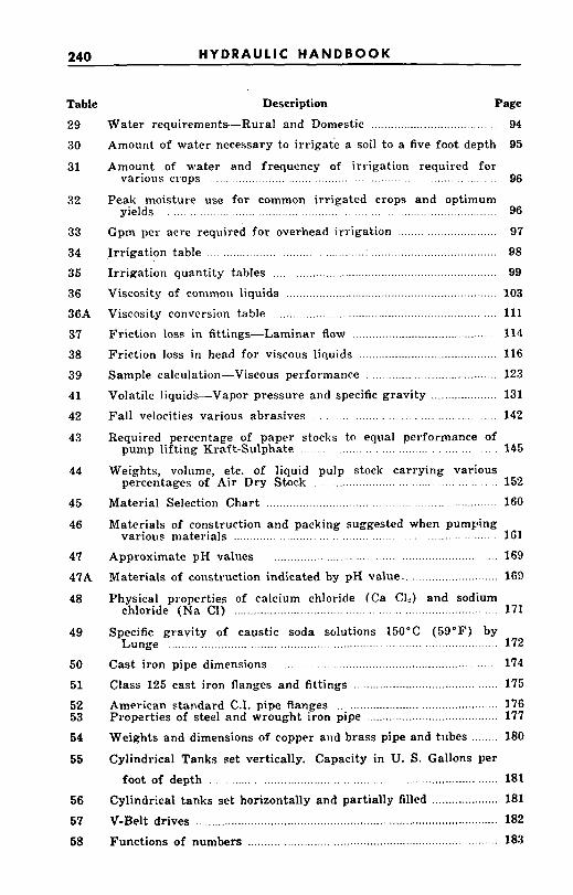
240 HYDRAULIC HANDBOOK
Table
29
30
31
32
33 34 35 36 36A 37 38 39 41 42
43
44
45
46
47 47 A 48
49
50 51 52 53
54
55
56
57
58
Description Page
Water requirements-Rural and Domestic . . ............................. 94 Amount of water necessary to irrigate a soil to a five foot depth 95
Amount of water and frequency of irrigation required for various crops . . . . . . . . . . . . . . . . . . . . . . . . . . . . . . . . . . . . . . . . . . . . . . . . . . . . . . . . . . . . . . . . 96
Peak moisture use for common irrigated crops and optimum
Gpm per acre required fo r overhead irrigation ............................
yields . . . . . . . . . . . . . . . . . . . . . . . . . . . . . . . . . . . . . . . . . . . . . . . . . . . . . . . . . . . . . . . . . . . . . . . . . . . . . . . 96
97 Irrigation table ......................................... : ...................................... 98 Irrigation quantity tables .................................................................. 99 Viscosity of common liquids ................................................................ 103
Viscosity conversion table ................................................................... 111
Friction loss in fittings-Laminar flow ........................................... 114 Friction loss in head fo r viscous liquids .......................................... 116 Sample calculation-Viscous performance ....................................... 123 Volatile liquids-Vapor pressure and specific gravity .................... 131 Fall velocities various abrasives . . . . . . . . . . . . . . . . . . . . . . . . . . . . . . . . . . . . . . . . 142
Required percentage of paper stocks to equal pcrformance of pump lifting Kraft-Sulphate . . . . . . . . . . . . . . . . . . . . . . . . . . . . . . . . . . . . . . . . . 145
Weights, volume, etc . of liquid pulp stock carrying various percentages of Air Dry Stock . . . . . . . . . . . . . . . . . . . . . . . . . . . . . . . . . . . . . . . . . . . 152
Material Selection Chart ................................................................. 160
Materials of construction and packing suggested when pumping various materials ..................................................................... 161
Approximate pH values .................................................................... 169 Materials of construction indicated by pH value ........................... 169
Physical properties of calcium chloride (Ca CIS) and sodium
Specific gravity of caustic soda solutions 150°C (59°F) by
Cast iron pipe dimensions ..........................................
Class 125 cast iron flanges and fittings ........................................... 175 American standard C.I. pipe flanges .............. ......................... 176 Properties of steel and wrought iron pipe ..... .......................... 177 Weights and dimensions of copper and brass pipe and t.ubes ........ 180
Cylindrical Tanks set vertically . Capacity in U . S . Gallons per
chloride ( N a C1) ........................................................................ 171
Lunge ............................................................................................. 172
foot of depth ...................................................................... 181
V-Belt drives ........................................................... ................. 182 Functions of numbers ........................................................................ 183
Cylindrical tanks set horizontally and partially filled .............
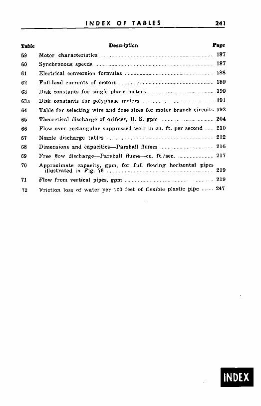
I N D E X OF T A B L E S 24 1
Table Description Page
59
60
61
62
63
63n
64
65
66
67
68
69
70
71
72
Motor characteristics ............................................................................ 187
Synchronous speeds ................................................................................ 187
Electrical conversion formulas ......... ............................... 188
Full-load currents of motors ................................................................. 189
Disk constants fo r single phase meters ..... .................................. 190
Disk constants fo r polyphase meters ......... .................................. 191
Table fo r selecting wire and fuse sizes for motor branch circuits 192
Theoretical discharge of orifices, U . S . gpm .................................. 204
Flow over rectangular suppressed weir in cu . f t . per second ...... 210
Nozzle discharge tables ................................................ ............... 212
Dimensions and capacities-Parshall flumes .................................... 216
Free flow discharge-Parshall flume-cu . ft./sec. ........................ 217
Approximate capacity, gpm, for full flowing horizontal pipes
Flow from vertical pipes, gpm .......................................................... 219
illustrated in Fig . 76 .................................................................... 219
Friction loss of water per 100 feet of flexible plastic pipe ........ 247
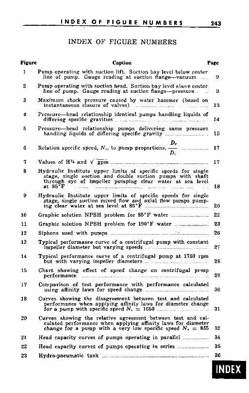
243 I N D E X O F F I G U R E N U M B E R S
INDEX O F FIGURE NUMBERS
Figure Caption Page 1
2
3
4
5
6
7 8
9
10 11 12 13
14
15
17
18
20
21 22
23
Pump operating with suction lift. Suction bay level below center line of punip. Gauge reading at suction Range-vacuum . . . . 9
Pump operating with suction head. Suction bay level above center line of pump. Gauge reading at suction flange-pressure . . . . . . . 9
Maximum shock pressure caused by water hammer (based on instantaneous closure of valves) ................................................... 13
Pressure-head relationship identical pumps handling liquids of differing specific gravities ............................................................ 14
Pressure-head relatiomhip pumps delivering same pressure handling liquids of differing specific gravity ............................. 15
D,
D, Relation specific speed, A'., to pump proportions, - ................... 17
Values of H?; and V gpm .................................................................... 17 -
Hydraulic Institute upper limits of specific speeds f o r single stage, single siiction and double suction pumps with shaft through eye of impeller pumping clear water at sea level a t 8 5 " F .......................................................................................... 18
Hydraulic Institute upper limits of specific speeds f o r single stage, single suction mixed flow and axial flow pumps pump- ing clear water at sea level a t 85°F ............................................
Graphic solution NPSH problem for 85°F water .......................... Graphic solution NPSH problem for 190°F water ........................ Siphons used with pumps ........................................... :.< .................... Typical performance curve of a centrifugal pump with constant
impeller diameter but varying speeds ..........................................
Typical performance curve of a centrifugal pump at 1750 rpm
Char t showing effect of speed change on centrifugal pi'mp performance ....................................................................................... 29
Comparison of test performance with performance calculated using aflinity laws fo r speed change ............................................ 30
Curves showing the disagreement between test and calculated performance when applying aiEnity laws fo r diameter change f o r a pump with specific speed N, = 1650 ....................................
Curves showing the relative agreement between test and cal- culated performance when applying affinity laws f o r diameter change fo r a pump with a very low specific speed N. = 855
20 22 23 26
27
but with varying impeller diameters ........... ............................ 28
31
32 Head capacity curves of pumps operating in parallel .................. 34
35 Hydro-pneumatic tank ..... .................................................. 36 Head capacity curves of pumps Operating in series ......................
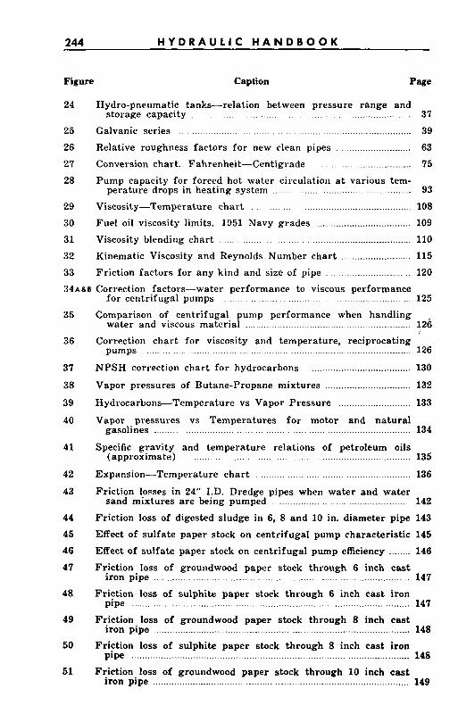
244 H Y D R A U L I C H A N D B O O K
Figure Caption Page
24 Hydro-pneumatic tanks-relation between pressure range and storage capacity ... .. .._.... ............._ .... ............._... ....................... 37
25 Galvanic series . ................. ...... . . . . . .......... ................................. 39
26 Relative roughness factors for new clean pipes .......................... 63
27 Conversion chart. Fahrenheit-Centigrade . . . . . . ..._ ...r.._..,.._.___._. 75
28 93
29 Viscosity-Temperature char t . .. .. . . . .........._...
30 Fuel oil viscosity limits. 1951 Navy grades _.....__..
31 Viscosity blending char t ..... ...... .. ... . . . ........._
32
33
34A&B Correction factors-water performance to viscous performance
Pump capacity for forced hot water circulation at various tem- perature drops in heating system . . . . . ....... ..._......... ........ ..........
Kinematic Viscosity and Reynolds Number char t ........................... 115
Friction factors for any kind and size of pipe . ............................ 120
fo r centrifugal pumps . . . . . . . ..,....._ . . ........ . .. . ....................... ... 125
35
36
37
38
39
40
41
42
43
44
45
46
47
48
49
50
51
Comparison of centrifugal pump performance when handling , water and viscous material _..,........ .. ................................... 126
Correction char t fo r viscosity and temperature, reciprocating
NPSH correction char t for hydrocarbons ....................................... 130
Vapor pressures of Butane-Propane mixtures ......................... Hydrocarbons-Temperature vs Vapor Pressure ............................ 133
Vapor pressures vs Temperatures f o r motor and na tura l gasolines _........ . .... .._......... ._....... ..... . ..... ._.... ... ... ...............___,___ 134
Specific gravity and temperature relations of petroleum oils (approximate) ........... .. . . . . . . ._ ._ . . . . . .__ ....__.. . .................................. 135
Expansion-Temperature cha r t ......... _ . ._ . ..... ...._... ....... ..........._._ 136
Friction losses in 24” I.D. Dredge pipes when water and water sand mixtures a re being pumped . _........_... ._ . _ _ _ _ ....___...__...._.... 142
Friction loss of digested sludge in 6, 8 and 10 in. diameter pipe 143
Effect of sulfate paper stock on centrifugal pump characteristic 145
Effect of sulfate paper stock on centrifugal pump efficiency .,_...._ 146
Friction.loss of groundwood paper stock through 6 inch cast iron pipe ................................................ . ...................... ...................... 147
Friction loss of sulphite paper stock through 6 inch cast iron pipe .__..__ .................................. ......._.._.__......_ .... ............................. 147
Friction. loss of ground d paper stock through 8 inch cas t iron pipe ......___.._..._...._._ ..................... ............................................. 148
Friction loss of sulphite paper stock through 8 inch cast iron pipe ................................................................................ _.__....___....__.._... 14s
Friction.loss of groundwood paper stock through 10 inch cast iron pipe ................................... .......... ....... .................................. ..._.._. 149
pumps , , . . . . . . .. . . . . . . . . . .. . . . . . . . . . . . . . . . . . . . . . . .. . . . . . .. . . . . . . .. .__. . . .._. . . . .
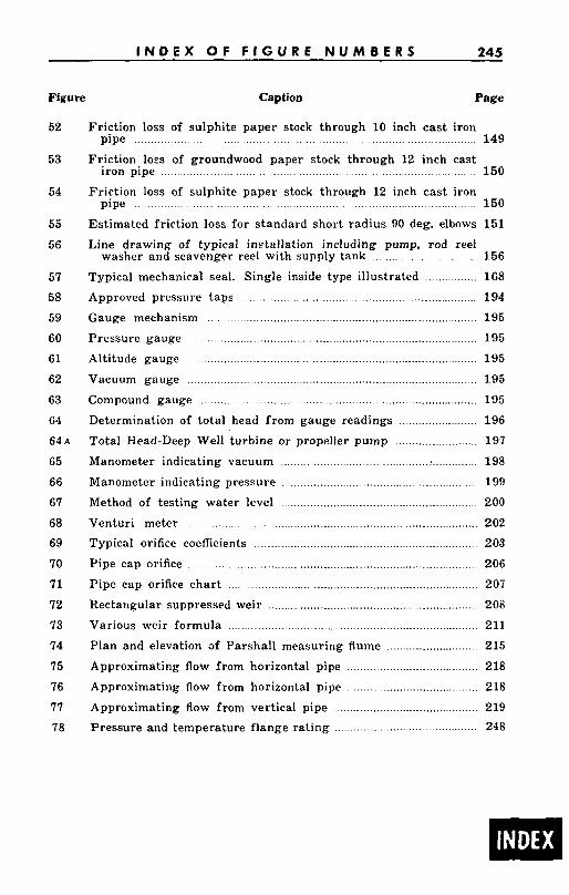
I N O E X O F F I G U R E N U M B E R S 245
Figure Caption Page
52
53
54
55 56
57 58 59 60
61 62 63 64 64 A
65 66 67 68 69 70 71 72 73 74 75 76 77 78
Friction loss of sulphite paper stock through 10 inch cast iron .................................................................................... 149 s of groundwood paper stock through 12 inch cast
iron pipe .............................................................................. 150 Friction loss of sulphite paper stock through 12 inch cast iron
pipe . . . . . . . . . . . . . . . . . . . . . . . . . . . . . . . . . . . . . . . . . . . . . . . . . . . . . . . . . . . . . . . . . . . . . . . . . . . . . . . . . . . . 150 Estimated friction loss for standard short radius 90 deg. elbows 151 Line drawing of typical installation including pump, rod reel
washer and scavenger reel with supply tank . . . . . . . . . . . . . . . . . . . 156 Typical mechanical seal. Single inside type illustrated ................ 168
Gauge mechanism .............................................................................. 195 Pressure gauge .................................... ......... 195 Altitude gauge ..................................................................................... 195 Vacuum gauge ........................... ..... 195 Compound gauge ................................................................................. 195 Determination of total head from gauge readings .......
Total Head-Deep Well turbine or propeller pump .......................... 197 Manometer indicating vacuum ........................................... : .............. 198 Manometer indicating pressure ............................................................ 199
Approved pressure taps ...................................................................... 194
Method of testing water level
Typical orifice coefficients ......
Pipe cap orifice char t ............ ................. 207 Rectangular suppressed weir ..
Various weir formula .............
Plan and elevation of Parshall measuring flume ............................ 215 Approximating flow from horizontal pipe .................... _ _ . _ _ _ 218 Approximating flow from horizontal pipe ..................................... 218
.. 219 Pressure and temperature flange rating ............................................ 248
.....................
Venturi meter ................................................................................. 202
Pipe cap orifice .....................
Approximating flow from vertical pipe . _ _
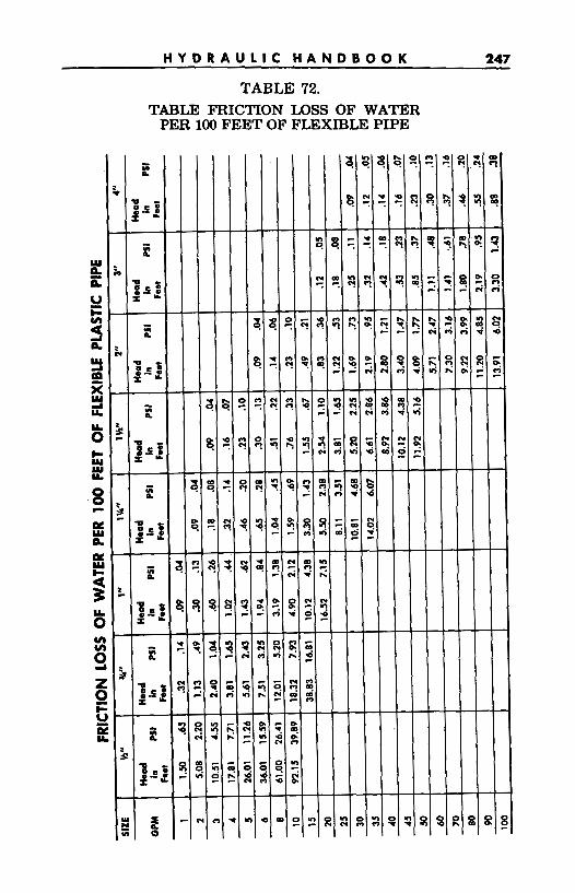
H Y D R A U L I C H A N D B O O K 247
TABLE 72. TABLE FRICTION LOSS OF WATER
PER 100 FEET OF FLEXIBLE PIPE
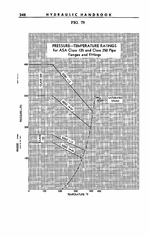
248 H Y D R A U L I C H A N D B O O K
FIG. 78

M E M O R A N D A

H Y D R A U L I C H A N D B O O K

M E M O R A N D A

H Y D R A U L I C H A N D B O O K

M E M O R A N D A
Directory of Operations
mFairbanks Morse Pump
CORPORATE HEADQUARTERS
Pentair, Inc. Waters Edge Plaza
1500 County Road 82 West St. Paul, MN 55113-3105
Phone: (612) 636-7920 Fax: (612) 639-5203
MANUFACTURING FACILITY
Fairbanks Morse Pump 3601 Fairbanks Avenue Kansas City, KS 66106 Phone: (913) 371 -5000
Fax: (913) 371-2272
PUMP SERVICES GROUP
Fairbanks Morse Pump 3601 Fairbanks Avenue Kansas City, KS 661 06 Phone: (913) 371-5000
Fax: (913) 371-0515

N O T E S


