69-70 NSTTUTE FOR RESEARCH ON ADJUSTED AND EXTENDED PRELIMINARY RESULTS FROM THE URBAN GRADUATED WORK INCENTIVE EXPERIMENT Harold W. Watts " i , " \ , . f", : J. '-l , , ':',' .!! ,,1_ : UNIVERSITY OF WISCONSIN - MADISON iW
Transcript
69-70
NSTTUTE FORRESEARCH ONPOVERTYD,scWl~~~~
ADJUSTED AND EXTENDED PRELIMINARY RESULTS FROM THE
URBAN GRADUATED WORK INCENTIVE EXPERIMENT
Harold W. Watts
"
i, " \
, . M"~I~f", : J. '-l
, , ':',',~,;;"i~,:i:7I'~'j.!!,,1_ :
~{ ~~UNIVERSITY OF WISCONSIN -MADISON iW
Revised June 10, 1970
ADJUSTED AND EXTENDED PRELIMINARY RESULTS FROM THE
URBAN GRADUATED WORK INCENTIVE EXPERIMENT
*by Harold W. Watts
General Description and Orientation of the Experiment
It is useful to review the objectives and structure of the Urban
Graduated Work Incentive Experiment, before going on to present and
interpret early results. The relevance of this experiment to the on-
going discussion of Nixon's Family Assistance Plan .and welfare reform
in general is genuine enough; but because it was planned and initiated
well before the introduction of legislation, and because it is still
along way from completion, these results must inevitably be both
less comprehensive and less powerful than many people would like them
to be, or think they should be.
The impact of welfare reform on the labor supply is both crucial
and poorly understood. First, if earned income goes down, the actual
benefit paid out will increase. This will raise the cost of the pro-
gram above the levels projected on the assumption of no change in in-
come, though not by the full amount of the drop in earnings. Secondly,
because any such income loss is only partially made up, the increase
in spendable income for the recipient of the benefit will be less than
that intended--i.e., less than the total amount of income before the
program plus the benefit. Consider the followi);J.g example: of a
given dollar paid out in benefits (at a fifty percent rate) ten cents
*Extensive credit for efforts underlying this report is due to DavidKershaw, Robinson Hollister, Jeri Fair, Felicity Skidmore and NancyWilliamson.
--~~-_._---- . -- ---------~._------------~
2
may in fact be offsetting a twenty-cent reduction in earnings, leav
ing the family only 80 cents better off than before. This would
compare with an expected benefit of 90 cents, all of which would
have represented increased spending power had there been no change
in earnings. Hence, reductions in income induced by the transter
system cut two ways; costs are 10 cents higher than expected and the
net impact on family income turns out to be 10 cents lower than ex
pected. This double-edged effect of disincentives on costs and
benefits makes accurate estimation of the earnings response crucial.
For many of the groups currently receiving the conventional wel
fare programs, large amounts of work and earnings have been neither
expected nor realized. An improved incentive structure for these
groups may elicit some small amount of additional effort; but for
precisely the reason that they were originally allowed to receive
transfers, it is unrealistic to expect that improvements beyond the
$33 1/3 of income they can now keep in most states will produce a
quantitatively significant increase in self support. The effect on
labor supply of the group that has not traditionally been eligible
for transfer payments (those working poor with appreciable if inade
quate incomes) may turn out to be significant, however. This group
represents proposed new beneficiaries who at present perform a sub
stantial amount of work. Their gainful work could well be discour
aged but we have no idea by how much. Therefore, the first priority
in an experiment that aims at ascertaining the labor supply response
to a major change in our transfer mechanism (and the consequent impact
on costs and benefits of such a program) must be to examine this group.
----_ .._~ ..~_._---~ -
3
This is the reasoning that led us to restrict our first experiment
to families (i) which include at least one dependent person and one
male between 18 and 58 where the male is neither disabled nor gqing
to school at the time of initial enrollment, and (ii) whose total~'(
family income is less than 150 percent of the "poverty line."
People have expressed concern that other important beneficiaries of
public assistance (the female~headed families, the aged, single per-
sons, etc.) were not included. In large part, this concern reflects
lack of appreciation of the difference between an experiment focussed
on a specific and pivotal issue and a demonstration or pilot program
aimed at a more holistic (and superficial) assessment of a proposed
program. It is not because the excluded groups are regarded as unim-
portant in general, nor that the kinds of reforms being proposed would
not provide major improvements in terms of dignity, equity, and even
'*The actual income levels used for determining eligibility are notthe same as the official poverty line~, but they are close. Our"poverty lines" are shown below along with the eligibility ceilingin terms of 1968 prices.
Family Size "Poverty Line" 150% of"Poverty Line"
2 2,000 3,000
3 2,750 4,125
4 3,300 4,950
5 3,700 5,550
6 4,050' 6,075
7 4,350 6,525
8 or more 4,600 6,900
4
incentives for these groups. It is rather that one important, well~
specified and as yet unclarified issue can be most appropriately ex-
plored by confining the study to the working--largely male-headed--
poor.
People have also been surprised to find the experiment not limited
entirely to families below the poverty line. But it must be clear
that any scheme that raises families up to or even close to the
poverty line and provides incentives for recipients to augment their
benefits must make partial payments to families well above the poverty
line. The Family Assistance Plan, for example, pays minimum benefits
of $1,600 for a family of four, but continues to pay fractional bene
*fits up to an earned income of $3,920. If the minimum benefit were
raised to, say, $2,400 the benefits schedule would extend up to earn-
ings of $5,520. There are many more working families in the $3,000-
$5,000 range than there are helow $3,000; and since these "near poor"
are directly affected by such a program it would be very foolish to
evaluate it on the basis of a minority among those who will be affected.
These restrictions on the eligible population do, certainly, limit
the value of the experiment for any holistic kind of evaluation. The
urban experiment in New Jersey and Pennsylvania is further limited by
concentrating on families in those parts of specific Eastern indus-
trial cities where poverty is most concentrated. Much of America's
*This amount is equal to twice the mlnlmum benefit (because of a 50percent tax rate) plus the $720 "set aside" of initial earnings thatdoes not reduce the benefit at all.
5
poverty population is in rural areas and smaller non-industrial towns.
And again much of it is scattered in parts of our metropolitan areas
outside the most ghetto-like environments.
This one experiment was simply not designed to provide direct
evidence on a random sample of poor families. It was designed to con
centrate on an important but more manageable group within which the
non-experimental variation was both less extreme and along fewer
dimensions. Other experiments are underway--in rural areas and in ,
urban areas with less exclusive sub-populations. But these are less
far along, with some, indeed, just getting underway. Bearing all these
limitations in mind, then, we may now consider a few key details of
the structure of the experiment.
The sample of households includes (a) control households who re
ceive no experimental transfers no matter how low their income goes
and (b) experimental households who are similar to the control house
holds in every way except that they are also eligible for payments
related to their income, under one of eight different variants of a
negative income tax. These eight differ as to (a) the maximum benefit
paid when income is zero, and (b) the rate at which benefits are re
duced as income increases; consequently they will also differ in terms
of (c) the break-even point, i.e., the level at which benefits finally
disappear. Some families at any time have incomes above the break-
even point for their particular program variant, and will therefore be
receiving no benefit. The control families, as well as the experi
mental families, can avail themselves of ordinary welfare and other
benefits provided by state or federal programs, although the experimental
6
families are required to forego benefits from the experimental pro-
gram if they receive cash welfare payments.
Every four weeks the experimental families (and not the controls)
are required to report their income and any changes in family size.
The benefit calculation is made at the central office; and if a bene-
fit is due, it is mailed to the family in two bi-weekly installments.
All of the families, however, are interviewed every three months;
and the data collected in this way (being comparable between control
and experimental families) is the basis for all controlled and scien~
tific comparisons. There are four experimental sites: Trenton,
Paterson-Passaic, Jersey City, and Scranton Pa. The magnitude of
work involved in finding and enrolling these households required
that the experimental sites be started up one at a time. Payments
were begun for the small (almost pilot) group in Trenton in August
1968. Paterson-Passaic did not come into operation until January
1969 followed by Jersey City in July and Scranton in October of the
same year.
The families:have been promised anonymity; they have also been
promised that, so long as they report their income to us accurately
and on time, they will remain eligible for payments based on their
income for a three-year period. It has been expected that families
will only gradually become adjusted to the program and the options
it provides. Moreover, it seems possible that their behavior will.
be affected by the approach of the end of the experiment to the
extent that they anticipate it. Thus, it may be that only a stretch
of data from the middle part of the experiment will reflect "normal"
behavior under a negative income tax program.
-------------------------------------
7
Selection and Assignment of Control and Experimental Treatments
The basis for measuring the effects of the eight negative tax
treatments on experimental families lies in the comparison between
the experimental group and the control group (null treatment) over
time. The extent to which these two groups exhibit different char-
acteristics at the time of enrollment on important variables such as
income, employment and family size may therefore be important in
interpreting the preliminary results. Using data from the screening
interview, we found no significant differences between these groups
in the urban experiment, allowing us to eliminate the possibility that
variations in response could be caused by the mismatch of control and
experimental groups on the basis of initial characteristics.
Experimental and control observations were selected randomly from
. )~
a stratified "poo.;L" of families who were judged eligible on the basis
of a screening and pre-enrollment interview (for eligibility criteria
see above). No attempt was made to "match" the experimental and con-
trol observations on the basis of any of the characteristics; observa-
tio~s assigned to each of the three income strata were randomly allo~
cated (using the RAND Corporation Tabie of Random Digits) to .the con-
trol group or to one of the eight negative tax plans. In Trenton,
Paterson and Passaic, 364 families were assigned to the experimental
treatments and 145 families to the control groMp.
*The three strata are: (i) family income below $3300/year for afamily of four; (ii) $330l/year to $4l25/year for a family of four;(iii) $4126 to $4950 for· a family of four. These levels are basedon revisions in the 1965 Social Security Administration poverty lines.
8
Tables 1 through 5 below compare the two groups for several criti-
cal variables, including summaries of initial characteristics both for
the 509 families from Trenton, Paterson and Passaic on which the OED.
report and the present study are based, and for the full sample of
*1218 (adding Jersey City and Scranton).
History of the February 18 Document
When the House Ways and Means Committee was in the final stages
of consideration of Nixon's Family Assistance Plan, the Office of
Economic Opportunity asked the Institute for a report on the first
indications from the urban experiment. At that point analysis of the
first returns had not yet been planned, let alone carried out. Only
a fraction of the eventual data base was available, and attempts to
draw conclusions from such a slim base would have been premature--
at least from the viewpoint of conventional scientific research.
Because of this opinion indeed, the development of a system for re-
cor:iHng, checking correcting, and finally analyzing the data had been
allowed to proceed slowly, and was only in an early stage of develop-
ment.
As soon as we began to consider how to respond to OED (at the·
very end of January), it became clear that a special crash effort was
required simply because the data and processing system being developed
for "normal" use would have taken at least two months to produce the
*This group does not include additional control families selectedsubsequently to bring the total sample to 1359.
Table 1: Racial Distribution
(Percentage)
Experimental
Trenton, Patersonand Passaic:
9
Control
BlackWhiteSpanish
Full sample:
BlackWhiteSpanish
44.613.042.0
38.632.828.6
47.512.040.0
30.94LO28.0
Table 2: Mean Years ofBchool Completed
Trenton, Patersonand Passaic:
Experimental
Control
Full sample:
Experimental
Control
7.96
7.46
8.63
8.69
*Table 3: Family Head Employed at Enrollment
(Percentage)
10
Trenton, Patersonand Passaic:
YesNo
Full sample:
YesNo
Experimental
89.011. 0
93.16.9
Control
93.76.3
94.15.9
*The difference in proportion unemployed at start is not largeenough to be significant at the .90 level (two-tailed test), although the "t" value is just short of the critical value in theTrenton, Paterson and Passaic subsamp1e.
Table 4: Mean Family Size at Enrollment
Trenton, Patersonand Passaic:
Experimental
Control
Full ·samp1e:
Experimental
Control
5.92 .
5.54
6.00
5.69
Table 5: Mean Fami Zy Earnings
(Year Preceding Enrollment)
Trenton, Patersonand Passaic:
11
Experimental
Control
Full sample:
Experimental
Control
$4,001
4,008
4,103
3,959
-------,
12
data instead of the two weeks we'had. Consequently, quick decisions
had to be made as to which variables would be of greatest interest and
also from which of the available interview waves these variables could
best be measured. It was possible to get observations spanning a full
year for Trenton; for Paterson-Passaic the available observations were
for nine months; and for the other cities the available time span was
felt to be too short to provide useful indications of any impact the
program might be having. Concentrating on the first two sites, then,
we chose to use the 9-month income changes in Paterson-Passaic and to
pool them with the 12-month changes for Trenton. Some information, of
course, was drawn from first, second, and third quarterlies for both
sites, as well as several items which were taken from the baseline or
pre-enrollment survey. These items were coded from the several sur
veys by recruiting a large number of people over one very busy week-end.
The coded data was punched in another rush operation, and then carried
from Princeton to Madison for tabulation and analysis. Machine tabu1a
tions proceeded through the first week of February. We encountered,
in the process, minor errors of punching and coding; but simply had no
time to trace them down and correct them if we were to meet the dead
line fprced upon us.
The following week personnel from Wisconsin and MATHEMATICA took
the raw tabulations to Washington, where a first draft of the report
was put together. In addition to the coded and processed data from the
questionnaires, two other sources of information were drawn upon for
the report: (i) some earlier tabulations of data from the screening
and pre-enrollment questionnaires that covered the entire sample (i.e.,
not just 'for Trenton and Paterson-Passaic), and (ii) income reports
13
submitted every four weeks by the experimental families only. These
income reports are valuable because they provide a more continuous and
comprehensive record of income than can be obtained from the question- ..
naires, which are only administered quarterly. They do not (of course)
provide any comparison!3 between experimental and control families.
Issues Concerning the Original Data Base
The most important and interesting issue about the experiment is,
as was stated above,the effect of the transfer treatment on labor
supply: i.e., the response of family earnings to the receipt of bene
fits. It was imperative that the OEO report addres!3 itself directly
to this problem. Table IV of that report, showing income changes for
control and experimental groups, represented our best efforts at that
point to answer the question: What do negative inqome tax payments
do to earnings of recipient family members?
The data behind that table were weekly incomes, measured by iden~
tical interviewing procedures for both control and experimental house
holds, at two points in time. We were concerned to make the interval
between measurements as lliong as possible, and to that end we used data
from the pre-enrollment and fourth quarterly interviews in Trenton
(which were administered in August of 1968 and 1969 respectively) and
data from the pre-enrollment and thi~d quarterlies ~or Paterson and
Passaic (administered in January and October 1969): This involved the
pooling of 9-month income changes for Paterson-Passaic with full-year
changes for Trenton. Given that there are controls in both places it
was not unreasonable to pool incQme changes for unequal intervals.
14
Longer intervals are, of course, better than shorter ones, and it is
now possible to incorporate data from the Paterson-Passaic fourth
quarterly and consider all the changes as referring to a one-year
interval. The new income change tables in this report are all based
on one~year changes.
A second problem is presented by the fact that a substantial
number of the families initially enrolled had been lost for a variety
of reasons, leading to the absence of any third or fourth quarterly
to provide income information for them. Eighty of the original 509
households were in this category for Trenton. An additional 18 were
lost in Paterson-Passaic between the third and fourth quarterlies.
This attrition is very troublespme--amounting to 19.3 percent of
the 509 original sample points during the first year of 9peration.
The attrition is understandably higher for controls than experimentals
(27 percent versus 16 percent); and it has been around 21 percent for
families with incomes too high to get benefits at the start. The rate
is also higher for the Spanish-speaking part of the sample (28 percent)
than for blacks and other whites (13 percent). It is, not surprisingly,
lowest among families that have started and remained eligible for
benefits above the minimum payments (8.3 percent).
In Trenton it is 22 percent and in Paterson-Passaic 18 percent.
The better experience in Paterson-Passaic may be attributable to (i)
higher base payments and also (ii) special efforts (introduced after
our initial experience in Trenton) to reduce attrition. Since most of
the Spanish-speaking people are in Paterson-Passaic, it seems likely
that the added efforts to cut down on attrition have been successful,
but partially offset by the inclusion of more Puerto Ricans. Within
15
the experimental group, the high tax rate plans show slightly more
attrition than the low ones; and the lower two income strata also have
a slightly higher rate of attrition than the upper one. Some of the
currently missing cases will be recovered, in the course of following
cases that have moved, etc., but there will be other new attrition
cases made up of those we can't find at the next interview. We shall
only know the final extent of the attrition when the interviewing
program is completed.
Besides cases of attrition, partially incomplete questionnaires
made it impossible to secure usable information on income change for
some families. Ideally, the income concept used for OEO's original
Table IV required that there be complete income information for the
husband and the wife from both the pre-enroilment and the subsequent
quarterly interview. Two different practices were used when any of
this information was missing:
1) If, on a given interview, income was reported properly·for one spouse but not for the other, the latter was assumed tobe zero. If neither spouse reported income, either at the earlyor later interview, the family was excluded from the analysis ofincome change. On this basis, 316 families provided usable income changes--84 control families and 232 experimental ones.Hence, in addition to the 80 families for whom the later interview was not available at all, another 103 were deleted becauseof incomplete income answers. These are the data that underlievariation I in the next section.
2) A second convention was used that permitted recovery ofmost of the 183 observations. If a spouse reported working inthe previous week (on a separate question) but did not provideearnings information, that component of income change was considered unusable; and the logic outlined in (1) above was followed. If, however, the previous question was either unansweredor answered with a non-work response, the earnings item was assumed to be zero. On this basis, 484 out of the 509 were usable-i.e., another 168 observations were salvaged. But these wouldnecessarily have a zero income total either for the earlier or
------ ------- -- ------
16
the later reading or both (40 in fact were zero both times).Nine more observations were rendered usable after correctionsof original card punching, and this produced the data baseunderlying variation III in the next section.
Neither of these two conventions are entirely satisfactory. The
first one excludes too many observations--cases where a zero income is
a reasonable guess. The second includes too many--namely the attrition
cases, for which no information at all was obtained from the fourth
quarterly. ,A middle ground has subsequently been adopted, which ex-
eludes cases with no fourth quarterly data and assigns zero for other
non-responses (except where there is evidence that one or both spouses
are working). This process yielded a total of 401 observations on
income change, which provide the data used for variations IV and V
below, and for the income change tables in the following section.
Updating and Extending Charts IV and V of the OED Preliminary ResultsReport of February 18, 1970.
As a previous section indicated, the OED Report was compiled
under considerable time pressure. Interviews used for analysis in-
eluded the pre-enrollment through the fourth quarterly in Trenton and
pr~-enrollment through the third quarterly in Paterson and Passaic.
We have subsequently had the opportunity both to correct coding and
punching errors in the original data cards and to increase th~ length
of the Paterson and Passaic experience by including the fourth quar-
terly interview.
The two most important entities in OED's Report are clearly
Charts IV and V: Chart IV specifying comparisons between experimental
17
and control groups in Trenton and Paterson-Passaic with regard to
changes in family incomes over time, and Chart V specifying the monthly
*mean incomes of experimental families in Pater$on and PassaIc only.
In Table VI, we shall present OEO' s Chart IV in its 'original
form (variation I) along with four close substitutes (only one of
which was available when the OEO Report was compiled).
Variation I (the one published in the report) was, as indicated
earlier, based on the 316 families which reported earnings (possibly
zero) on both the earlier and later interviews for at least one
spouse. It was also based on data cards that contained minor coding
and punching errors; and the l2-month changes from Trenton were pooled
with the 9~month changes for Paterson~Passaic.
Families were cross-classified jointly by their pre-experiment
earnings and their later earnings using intervals (of weekly earnings)
as follows: 0; $1-25; $26-50; $51-65; $66-80; $8l-95;$96~110;
$111-125; $126-150; $151 or more.
Income was regarded as having changed for any family found in a
different earnings interval for the later interview than for the
earlier one. On average this required a change of at least $15/week
in the middle of the observed earning distribution.
Variation II is based on the same procedure as Variation I, the
only difference being that the errors in the data cards were corrected.
*Trenton was not included in Chart V primarily because of difficultiesin handling the different time periods covered in the two sites. Itcould be included, however, without changing the direction of the trendshown in the chart.
18
Table 6: Comparisons between Experimental and Control Groupswith Regard to Changes in Family Earnings Over Time
Variation:(:1 --Original Report: Trenton Fourth Quarterly and Patersonand Passaic Third Quarterly (Coding. errors uncorrected; all non~
responses eliminated; N = 316)
Percent of families whose:
Earnings increasedEarnings did not changeEarnings declined
Control
43%2631
Experimental
53%1829
Variation II ~-Trenton Fourth Quarterly and Paterson and Passaic ThirdQuarterly (Data cards corrected; all non-responses eliminated, N = 318)
Percent of families whose:
Earnings increasedEarnings did not changeEarnings declined
44%2432
55%1827
Variation III ~-Trenton Fourth Quarterly and Paterson and Passaic ThirdQuarterly (Data cards corrected; non-responses analyzed to add in zeroincomes; significant at 95 percent level of confidence; N =493)
Percent of Families whose:
Earnings increasedEarnings did not changeEarnings declined
31%2544
43%1938
Variation IV --Trenton Fourth Quarterly and Paterson and Passaic FourthQuarterly (Data cards corrected; families required to move out ofinterval $25 wide to show increase or decrease; attrition cases eliminated, other non-responses set equal to zero; N'= 401)
Percent of families whose:
Earnings increasedEarnings did not changeEarnings decreased
34%3729
33%3928
Variation V --Trenton Fourth Quarterly and Paterson and Passaic FourthQuarterly (Data cards corrected; families required to move out ofinterval $15 wide to show increase or decrease~ attrition caseseliminated, other non-responses set equal to zero; N = 400)
Percent of families whose:
Earnings increasedEarnings did not changeEarnings decreased
--------------~.~~-----
41%2930
43%2829
19
Two additional cases were usable and the percentage distribution was
changed only slightly.
Variation III shows the corrected data; but the alternative pro
cedure outlined above was used to assign zero incomes to most of the
non-response cases. This made a total of 493 "usable" records (97
percent). With the larger sample, the greater percentage of increases
among experimentals become significant at the .05 level. A comparable'
table was computed while preparing the OED Report using the uncorrected
cards and was, again, only trivially different from this one.
Variations IV and V are based on a more drastically improved
data base. Fourth quarterly earnings have replaced third quarter~y
earnings for the Paterson-Passaic families (these were not available
earlier), and all (98) that have not (as yet) completed the fourth
quarterly interview have been eliminated. The 410 observations
remaining (one family that had split was entered twice in the original
509 cases), were then processed using the zero-assignment procedure
when a head or spouse was not known to have been working. This pro
cess eliminated 9 families in which someone was working but no earn
ings were reported. For each of the remaining 401 families, the change
in earnings over the year since the experiment started was explicitly
calculated rather than inferred from a cross-tabulation. From the
distribution of changes so calculated, Variation IV displays the
percentage breakdowns for (a) increases of $25/week or more, (b) no
change (plus or minus) as great as $25/week and (c) decreases of
$25/week or more. Using these procedures there is virtually no dif
ference between the experience of control and experimental families-..,.
---~-~.-----~
20
the latter had one percent fewer increases but also one percent few
er decreases.
For variation V, a narrower interval was used for "no change."
Changes of $15/week or more were counted. This produced a substantial
increase in positive 'changes and very little change (one percent) in
the number of decreases counted. Here the experimental families had
more increases and fewer decreases--but even so, the differences do
not approach statistical significance.
Of the first three variations, which relate to the data used for
the original report (except for correcting minor errors) variation
III provides the strongest indication of greater effort, as reflected
in earnings, for experimental families. Almost all families are re
presented, and the data have been purged of minor errors. The result
ing differences in that table are significant at the .05 level (i.e.,
would happen only one time out of 20 purely by chance if there were no
real difference between controls and experimental changes in earnings).
Variation I was used in the original report rather than (the uncor
rected version of)'Variation III for two reasons. First, it involved
no assignment of values to non-response--and was "conservative" in that
sense. Second, since there were, and are, ample reasons for being
cautious in interpreting these early data, a non-significant and less
marked contrast between control and experimental families, as provided
in Variation I (or II), was preferred for immediate release--again with
the aim of making a conservative choice.
The last two variations, which are based on a third approach to
the non-response problem and use data for full-year changes in earnings
I! 21
in both cities show no significant differences. There is some effectI
that depends on the required size of earnings changes however. For
~eference it may be useful to note that a $15/week change of earnings
of head and spouse corresponds to about 20 percent of average earnings
at enrollment, and a $25/week change corresponds to 33 percent of
average earnings at enrollment. The actual average increase over the
year was around 7 percent, broken down as shown below in Table 7.
Table 7: WeekZy Mean Average FamiZy Earnings
Enrollment
Fourth Quarterly
Percentage Change
Control
$74.87
79.84
6.6%
Experimental
$77.74
83.52
7.4%
The original report's Chart V has now been updated, thereby elimi-
nating two small problems with the original data. There were minor
entry errors in the raw data tables used to calculate the chart, and
the final summation of Paterson and Passaic mean family incomes was
not weighted correctly (data went to OEO for Chart V in six parts--mean
incomes for each of the three incomes strata in each city--which were
not properly weighted when added to get a total monthly mean income).
Neither of these errors had any appreciable impact on the Chart and the
conclusions obviously remain the same. In addition to the above' correc-
tions, the chart has now been extended to include two additional months,
bringing it to a full year. Comparisons between the original and the
updated and extended monthly means are shown below (Table 8):
Table 8: COY'Y'ected and Updated VeY'$ions of the Cha:rt Vin OED's DY'iginaZ Rep0Y't
Original Updated and Extended
Month 1 $340 332
Month 2 361 361
Month 3 3~8 379
Month 4 383 383
Month 5 381 372
Month 6 380 386
Month 7 363 355
Month 8 358 356
Month 9 385 370 .
Month 10 381 375
Month 11 383
Month 12 391
22
23
The Paterson-Passaic experimental group was used alon~ in OED's
original chart, because their report had to be short and easy to under-~'(
stand and Trenton could not be "added in" in any simple or obvious way.
Trenton started five months earlier and had been running longer, but
there were many more observations in the Paterson-Passaic group, making
the trend, though shorter, more reliable. In any case, since there are
no comparable measures for the control group, Chart V can only be in-
terpreted relative to general knowledge of income experience of the
poor. Within this frame of reference, both Chart V and the comparable
diagram for Trenton (or even for subgroups such as income strata) are
equally emphatic in showing that there is no pronounced reduction in
incomes following enrollment in our benefit program.
Further Tests and Analysis
This section presents more complete results for the subgroup of
410 families from Trenton, Paterson and Passaic from whom we have usable
fourth quarterly questionnaires.
As regards the analysis of change in earnings, the discussion here
will concentrate on earnings changes greater than $25/week. Similar
tests and tables were compiled using the $15/week criterion but, since
they generally gave the same indications (and were similarly non-sig-
nificant) :they are deleted here. In addition to changes in total
earnings of head and spouse (called family earnings above) changes in
*For instance, should one combine the 'same calendar month, as closelyas possible, or months that are equidistant from the beginning ofbenefit payments?
II
I
I----_-!
24
earnings of the head alone have been analyzed and are presented below,
again considering only changes greater than $25/week.
The earnings changes of families or heads were classified accord
ing to treatment--both the gross control/experimental contrast and
distinguishing among treatments within the experimental groups (Tables
9 and 10). Chi-square contingency tests were carried out, and in no
case was the null hypothesis of no difference in earnings change among
groups rejected at the .10 level (a less stringent requirement than
the .05 level typically used for such tests). Classifications by city,
ethnic group and stratum were also made (Tables 11 and 12). The only
instance of significance at the .10 level was for husband's earnings
change for the contrast between Trenton and Paterson-Passaic; here
most of the difference between the two cities was found in the experi
mental groups.
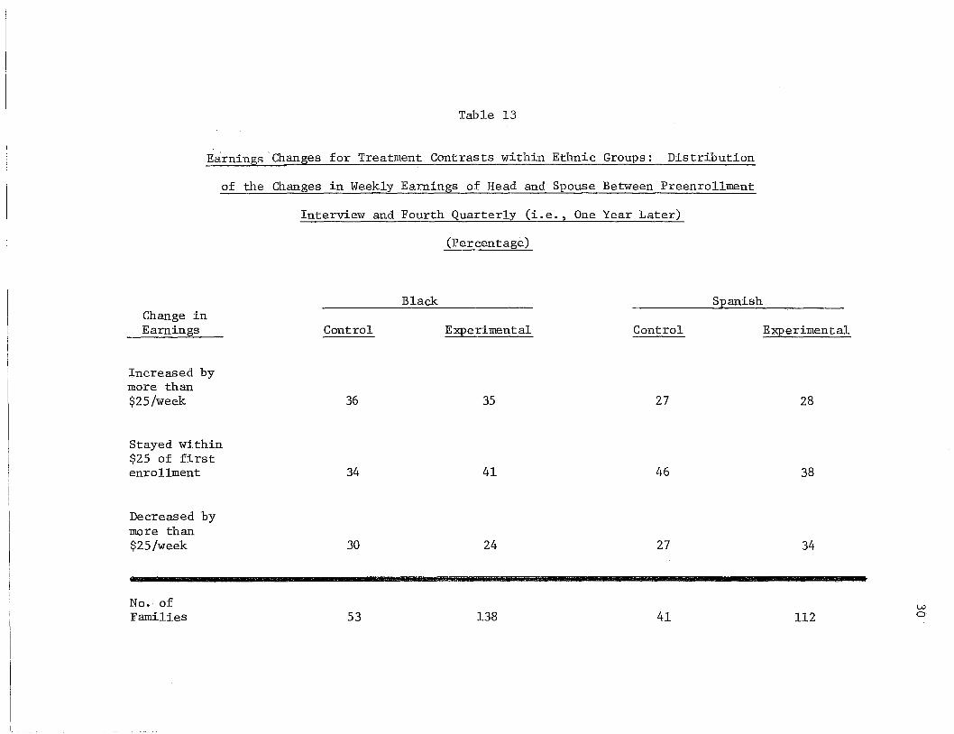
When control/experimental comparisons were made within black and
Spanish subgroups, there was a nearly-significant relation between the
treatment and city classification and change in total family earnings.
Most of this was due to a sharp difference between the two experimental
subgroups (Table 13).
In Table 14 the control/experiment comparisons are shown within
the two cities for earnings of the head alone. As will be noted, most
of the favorable evidence for the experimental group comes from a dis~
proportionate number of earnings increases in Paterson-Passaic.
Even though the other differences are not statistically signifi"':
cant, it will be useful to discuss further the patterns of income change·
shown in Tables 9-14.
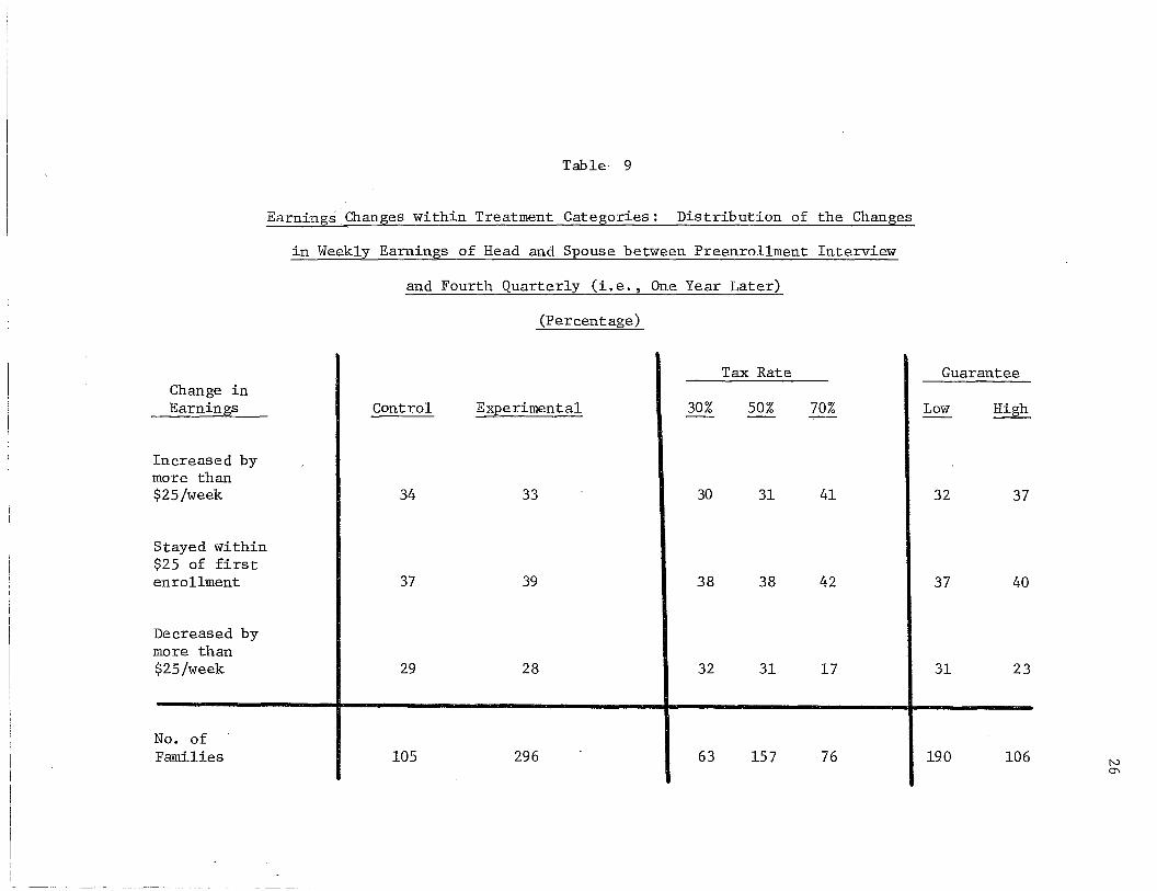
25
Table 9 shows the distribution of earnings changes for the con
trol and experimental groups and, within the experimentals, .for tax
rate and guarantee level. With the change to a more satisfactory data
base, the distribution of changes in earnings is virtually identical
between controls and experimentals when one considers the earnings of
head and spouse combined. Higher tax rates appear to elicit more earn
ings increases in this table, as do high guarantees. But it must be
emphasized that these differences are not significant. Table 10 shows
the same comparison for earnings of the head only. Here heads of ex
perimental families show up slightly better than controls; but otherwise
the picture is much the same, and again not significant.
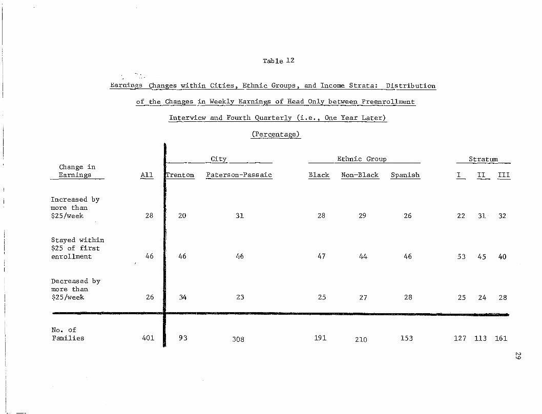
Tables 11 and 12 show the change distributions for the total sample
and for the two different cities (or experimental sites) for ethnic
groups and for income strata. Paterson-Passaic shows a greater preval
ence of earnings increases and fewer decreases both for the earnings of
head and for head and spouse combined. The differences are significant
at the 90 percent level for head's earnings. The sample is then split
into two parts--black and non-black--and a separate column is shown for
the Spanish-speaking (overwhelmingly Puerto Rican) portion of the non
black group. For changes in head's earnings (Table 12) there is scarcely
any discernible difference. What little there is shows the blacks
having fewer decreases in earnings. Considering combined income of
head and spouse, the experience of the black families shows a more pro
nounced (but not yet significant at the 90 percent level) tendency
toward earnings gains as compared to the rest of the sample. The con-
trasts by stratum mainly show a tendency for the higher strata to have
Table· 9
Earnings Changes within Treatment Categories: Distribution of the Changes
in Weekly Earnings of Head and Spouse between Preenrollment Interview
and Fourth Quarterly (i.e., One Year Later)
(Percentage)
Tax Rate GuaranteeChange inEarnings
Increased bymore than$25/week
Stayed within$25 of firstenrollment
Decreased bymore than$25/week
No. ofFamilies
Control
34
37
29
105
Experimental
33
39
28
296
30%
30
38
32
63
50%
31
38
31
157
70%
41
42
17
76
Low
32
37
31
190
High
37
40
23
106 N~
I
Table 10
Earnings Changes within Treatment Categories: Distribution of Changes
in Weekly Earnings of Head Only between Preenrollment Interview and
Fourth Quarterly (i.e., One Year Later)
(Percentage)
Change inEarnings
of Head Control Experimental
Tax Rate
30% 50% 70%
Guarantee
Low High
Increased bymore than$25/week
Stayed within$25 of firstenrollment
Decreased bymore than$25/week
No. ofFamilies
24
49
27
105
30
44
26
296
27
43
30
63
28
45
27
157
37
45
18
76
28
44
28
190
33
45
22
106N-....J
Table 11
Earnings Changes within Cities, Ethnic Groups, and Income Strata: Distribution
of the Changes in Weekly Earnings of Head and Spouse between Preenrollment
Interview and Fourth Quarterly (i.e., One Year Later)
(Percentage)
City Ethnic Group StratumChange in
-
Earnings All I Trenton Paterson-Passaic Black Non-Black Spanish I II III