1

Title: Physical density estimations of single- and dual-energy CT using material-based forward 1

projection algorithm 2

Running Title: Physical density estimations using material-based forward projection 3

4

Author: 5

Kai-Wen Li1,2, Daiyu Fujiwara3, Akihiro Haga3a, Huisheng Liu1 and Li-Sheng Geng2,1,4,5 6

1. Beijing Advanced Innovation Center for Big Data-Based Precision Medicine, School of Medicine 7

and Engineering, Beihang University, Key Laboratory of Big Data-Based Precision Medicine 8

(Beihang University), Ministry of Industry and Information Technology, Beijing 100191, China 9

2. School of Physics, Beihang University, Beijing 102206, China 10

3. Graduate School of Biomedical Sciences, Tokushima University, Tokushima 770-8503, Japan 11

4. Beijing Key Laboratory of Advanced Nuclear Materials and Physics, Beihang University, Beijing 12

102206, China 13

5. School of Physics and Microelectronics, Zhengzhou University, Zhengzhou, Henan 450001, China 14

15

Corresponding Author: 16

Akihiro Haga, Ph.D. 17

Electronic mail: haga@tokushima-u.ac.jp 18

Telephone number: +81 88 633 9024 19

Mailing address: 3-18-15 Kuramoto-cho, Tokushima, 770-8503, Japan 20

21

2

Abstract 22

Purpose: This study aims to evaluate the accuracy of physical density prediction in single-energy CT 23

(SECT) and dual-energy CT (DECT) by adapting a fully simulation-based method using a material-24

based forward projection algorithm (MBFPA). 25

Methods: We used biological tissues referenced in ICRU Report 44 and tissue substitutes to prepare 26

three different types of phantoms for calibrating the HU-to-density curves. Sinograms were first 27

virtually generated by the MBFPA with four representative energy spectra (i.e. 80 kV, 100 kV, 120 kV, 28

and 6 MV) and then reconstructed to form realistic CT images by adding statistical noise. The HU-to-29

density curves in each spectrum and their pairwise combinations were derived from the CT images. The 30

accuracy of these curves was validated using the ICRP110 human phantoms. 31

Results: The relative mean square errors (RMSEs) of the physical density by the HU-to-density curves 32

calibrated with kV SECT nearly presented no phantom size dependence. The kV-kV DECT calibrated 33

curves were also comparable with those from the kV SECT. The phantom size effect became notable 34

when the MV X-ray beams were employed for both SECT and DECT due to beam hardening effects. 35

The RMSEs were decreased using the biological tissue phantom. 36

Conclusions: Simulation-based density prediction can be useful in the theoretical analysis of SECT 37

and DECT calibrations. The results of this study indicated that the accuracy of SECT calibration is 38

comparable with that of DECT using biological tissues. The size and shape of the calibration phantom 39

could affect the accuracy, especially for MV CT calibrations. 40

Keywords: CT calibration, Dual-energy CT, Biological tissue, ICRP110 human phantom, HU-to-41

density curve 42

43

Introduction 44

To establish the relationship between the computed tomography (CT) number (in Hounsfield units, 45

HU) of a given voxel and the physical (or electron) density relative to water is one of the crucial 46

processes that control the variance of patient dose calculations in radiotherapy treatment planning1-3. 47

The HU-to-density conversion is typically determined by calibration curves, which are experimentally 48

3

obtained from tissue-substitutes with known densities in a calibration phantom. Several studies have 49

investigated the sensitivity of dose calculation for photon and particle beams relative to the accuracy of 50

this conversion4-7. A major concern of this approach is that the elemental composition of these substitutes 51

may differ from that of biological tissues, and consequently, the adopted calibration curves may not be 52

sufficiently accurate. One way to overcome this problem is the state-of-the-art stoichiometric calibration 53

method introduced by Schneider et al.8, in which the specific parameters of a CT scanner are determined 54

by the measurement of a few tissue-substitutes with known materials. Recently, this method has been 55

re-examined in the context of single-energy CT (SECT) calibration for proton therapy treatment 56

planning, and its accuracy was found to depend on the tissue-substitutes used for calibration9. This 57

dependency implies that the improvement of dual energy CT (DECT) over SECT should also be re-58

assessed, which may depend on the use of tissue substitutes as determined in a number of experiments 59

for predicting relative stopping powers in proton therapy10. 60

In this study, the accuracy of physical density prediction using SECT and DECT was evaluated, which 61

is the first step in treatment planning. To reduce the uncertainty of the calibration, the HU-to-density 62

conversion using biological tissues from ICRU Publication 44 was proposed11-15. The approach in this 63

study differs from the stoichiometric calibration8 by assuming that the X-ray spectra are known for the 64

evaluation of the attenuation coefficients. In this case, CT values were reconstructed from the sinograms 65

generated by the material-based forward projection algorithm (MBFPA), which has been utilised in 66

model-based material decomposition16,17, when the material composition of the object was determined. 67

These CT values were then used to perform the calibration to obtain the HU-to-density look-up-table 68

(LUT). Using this LUT, arbitrary CT images can be converted to density images. Namely, this approach 69

is a full simulation of the clinical process because it is based on the modelling of the entire CT system, 70

including the incident X-ray energy spectrum. 71

The aim of this study was threefold. First, the feasibility of the proposed approach using MBFPA for 72

physical density prediction was presented, which is significantly relevant to estimate proton stopping 73

powers for treatment planning. To achieve this, the HU-to-density curves were simulated using three 74

types of phantoms, where phantom (size/shape and composition) dependence in the calibration was also 75

analysed. Second, the advantage of DECT over SECT for calibrations based on the proposed approach 76

4

was quantitatively evaluated. Furthermore, the issue of whether a large energy gap in DECT, such as in 77

the kilovoltage-megavoltage (kV-MV) range, could improve the accuracy of estimating the physical 78

density was reassessed. 79

Materials and Methods 80

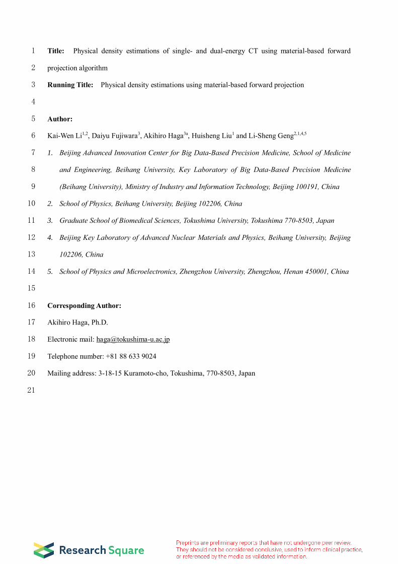
The schematic workflow is shown in Fig. 1. The method starts with the preparation of three types of 81

two-dimensional material-based digital calibration phantoms. Next, virtual projections (or sinograms) 82

were produced using MBFPA, and CT images were sequentially reconstructed with the sinograms. 83

Using the reconstructed images, the HU-to-density LUTs were calculated for each phantom. Finally, 84

these LUTs were validated by predicting the physical density distributions of the ICRP110 human 85

phantom. Four different X-ray energy sources (i.e. 80 kV, 100 kV, 120 kV, 6 MV) were employed. Thus, 86

four SECTs and their six pairwise combinations for DECTs were considered. 87

88

89

Fig. 1. Workflow of the current study for total density evaluation. BT(A), TS, and BT(B) phantoms were used for

the calibration, and the ICRU human phantoms were used for the validation (for more details, see the main text).

5

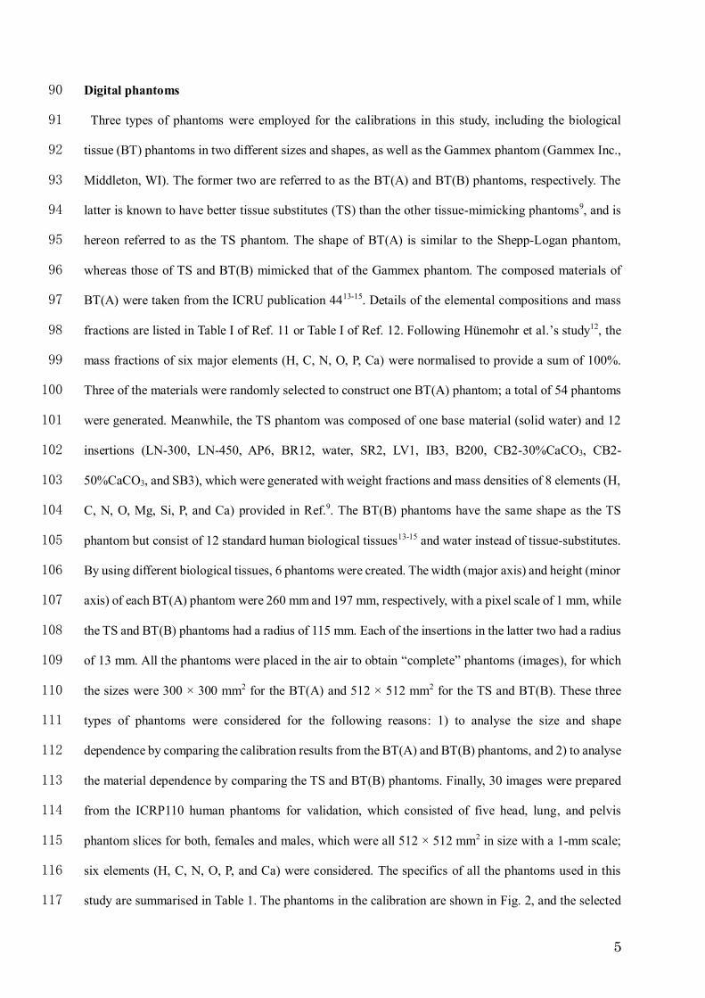
Digital phantoms 90

Three types of phantoms were employed for the calibrations in this study, including the biological 91

tissue (BT) phantoms in two different sizes and shapes, as well as the Gammex phantom (Gammex Inc., 92

Middleton, WI). The former two are referred to as the BT(A) and BT(B) phantoms, respectively. The 93

latter is known to have better tissue substitutes (TS) than the other tissue-mimicking phantoms9, and is 94

hereon referred to as the TS phantom. The shape of BT(A) is similar to the Shepp-Logan phantom, 95

whereas those of TS and BT(B) mimicked that of the Gammex phantom. The composed materials of 96

BT(A) were taken from the ICRU publication 4413-15. Details of the elemental compositions and mass 97

fractions are listed in Table I of Ref. 11 or Table I of Ref. 12. Following Hunemohr et al.’s study12, the 98

mass fractions of six major elements (H, C, N, O, P, Ca) were normalised to provide a sum of 100%. 99

Three of the materials were randomly selected to construct one BT(A) phantom; a total of 54 phantoms 100

were generated. Meanwhile, the TS phantom was composed of one base material (solid water) and 12 101

insertions (LN-300, LN-450, AP6, BR12, water, SR2, LV1, IB3, B200, CB2-30%CaCO3, CB2-102

50%CaCO3, and SB3), which were generated with weight fractions and mass densities of 8 elements (H, 103

C, N, O, Mg, Si, P, and Ca) provided in Ref.9. The BT(B) phantoms have the same shape as the TS 104

phantom but consist of 12 standard human biological tissues13-15 and water instead of tissue-substitutes. 105

By using different biological tissues, 6 phantoms were created. The width (major axis) and height (minor 106

axis) of each BT(A) phantom were 260 mm and 197 mm, respectively, with a pixel scale of 1 mm, while 107

the TS and BT(B) phantoms had a radius of 115 mm. Each of the insertions in the latter two had a radius 108

of 13 mm. All the phantoms were placed in the air to obtain “complete” phantoms (images), for which 109

the sizes were 300 × 300 mm2 for the BT(A) and 512 × 512 mm2 for the TS and BT(B). These three 110

types of phantoms were considered for the following reasons: 1) to analyse the size and shape 111

dependence by comparing the calibration results from the BT(A) and BT(B) phantoms, and 2) to analyse 112

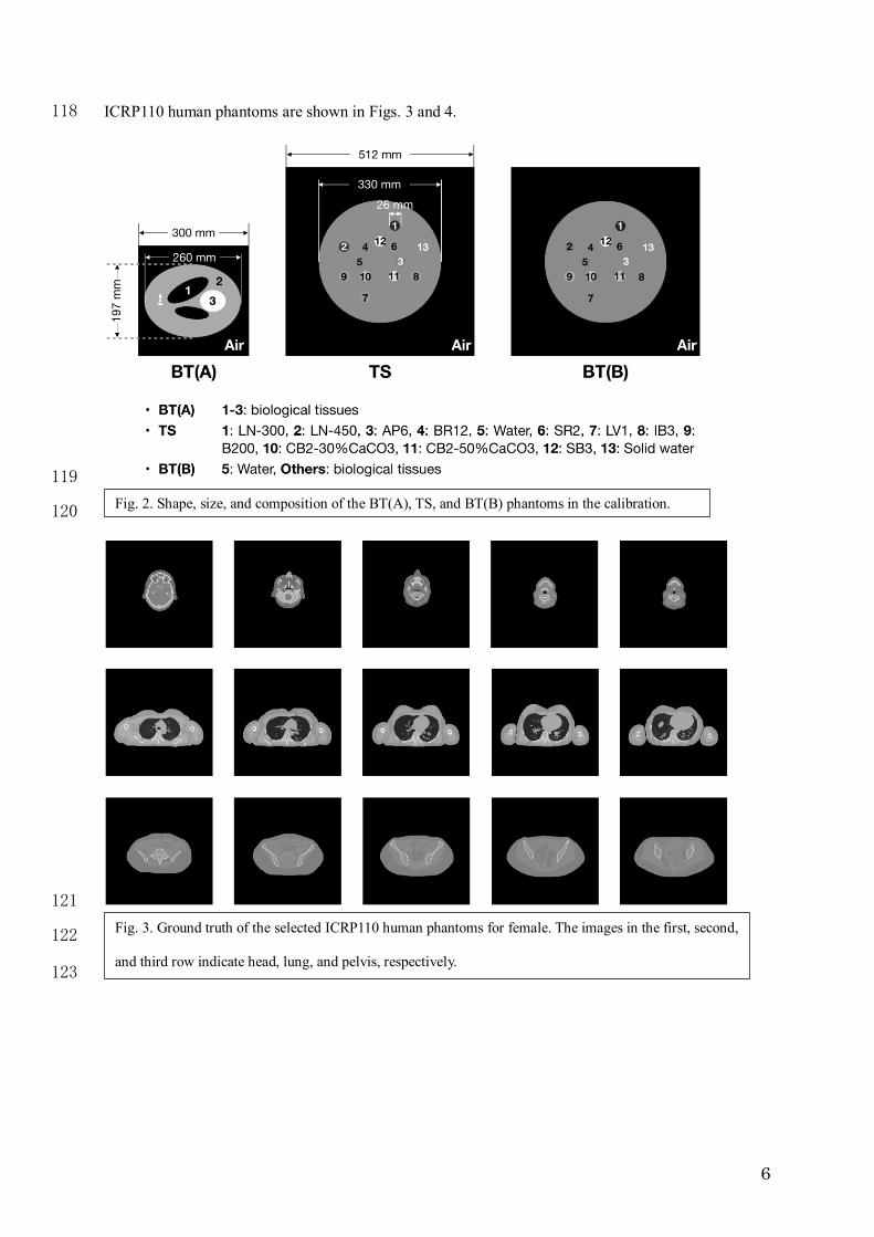
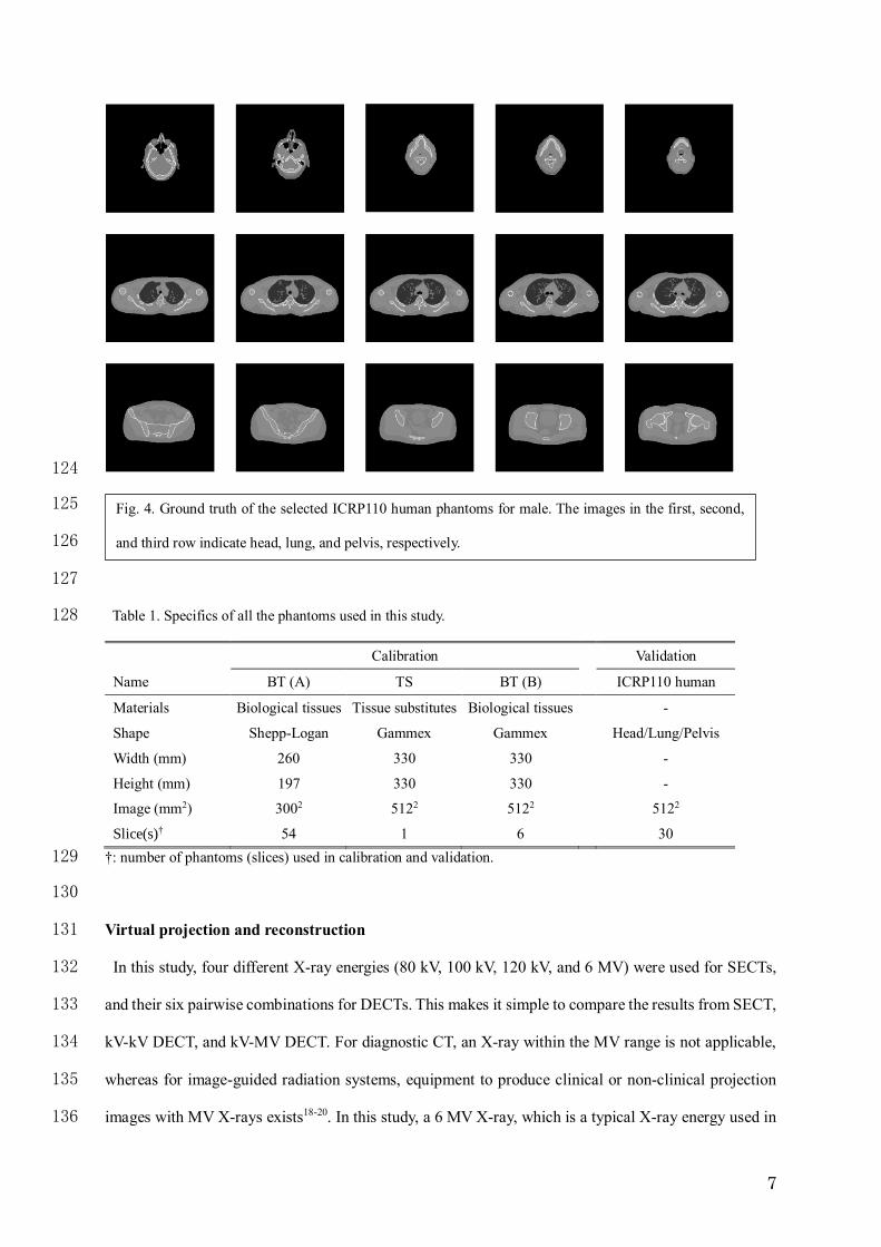
the material dependence by comparing the TS and BT(B) phantoms. Finally, 30 images were prepared 113

from the ICRP110 human phantoms for validation, which consisted of five head, lung, and pelvis 114

phantom slices for both, females and males, which were all 512 × 512 mm2 in size with a 1-mm scale; 115

six elements (H, C, N, O, P, and Ca) were considered. The specifics of all the phantoms used in this 116

study are summarised in Table 1. The phantoms in the calibration are shown in Fig. 2, and the selected 117

6

ICRP110 human phantoms are shown in Figs. 3 and 4. 118

119

120

121

122

123

Fig. 2. Shape, size, and composition of the BT(A), TS, and BT(B) phantoms in the calibration.

Fig. 3. Ground truth of the selected ICRP110 human phantoms for female. The images in the first, second,

and third row indicate head, lung, and pelvis, respectively.

7

124

125

126

127

Table 1. Specifics of all the phantoms used in this study. 128

Calibration Validation

Name BT (A) TS BT (B) ICRP110 human

Materials Biological tissues Tissue substitutes Biological tissues -

Shape Shepp-Logan Gammex Gammex Head/Lung/Pelvis

Width (mm) 260 330 330 -

Height (mm) 197 330 330 -

Image (mm2) 3002 5122 5122 5122

Slice(s)† 54 1 6 30

†: number of phantoms (slices) used in calibration and validation. 129

130

Virtual projection and reconstruction 131

In this study, four different X-ray energies (80 kV, 100 kV, 120 kV, and 6 MV) were used for SECTs, 132

and their six pairwise combinations for DECTs. This makes it simple to compare the results from SECT, 133

kV-kV DECT, and kV-MV DECT. For diagnostic CT, an X-ray within the MV range is not applicable, 134

whereas for image-guided radiation systems, equipment to produce clinical or non-clinical projection 135

images with MV X-rays exists18-20. In this study, a 6 MV X-ray, which is a typical X-ray energy used in 136

Fig. 4. Ground truth of the selected ICRP110 human phantoms for male. The images in the first, second,

and third row indicate head, lung, and pelvis, respectively.

8

radiation treatment, was selected. The spectra of the X-ray sources were obtained by Monte-Carlo (MC) 137

simulations using the GEANT4 toolkit (version 10.4) for a linear accelerator with kV imaging capability 138

(Synergy, Elekta, UK). For kV X-rays, low-energy photons generated from an anode were decimated 139

by filters composed of aluminium and copper, and the beam shape was formed by lead-cone and cassette 140

collimators. For the MV X-rays, the photons generated from the target were decimated by a flattening 141

filter, and the beam shape was formed by primary, jaw, and multi-leaf collimators. In both cases, the 142

energy spectrum was formed by the photons collected on the plane located 70 cm from the sources21. 143

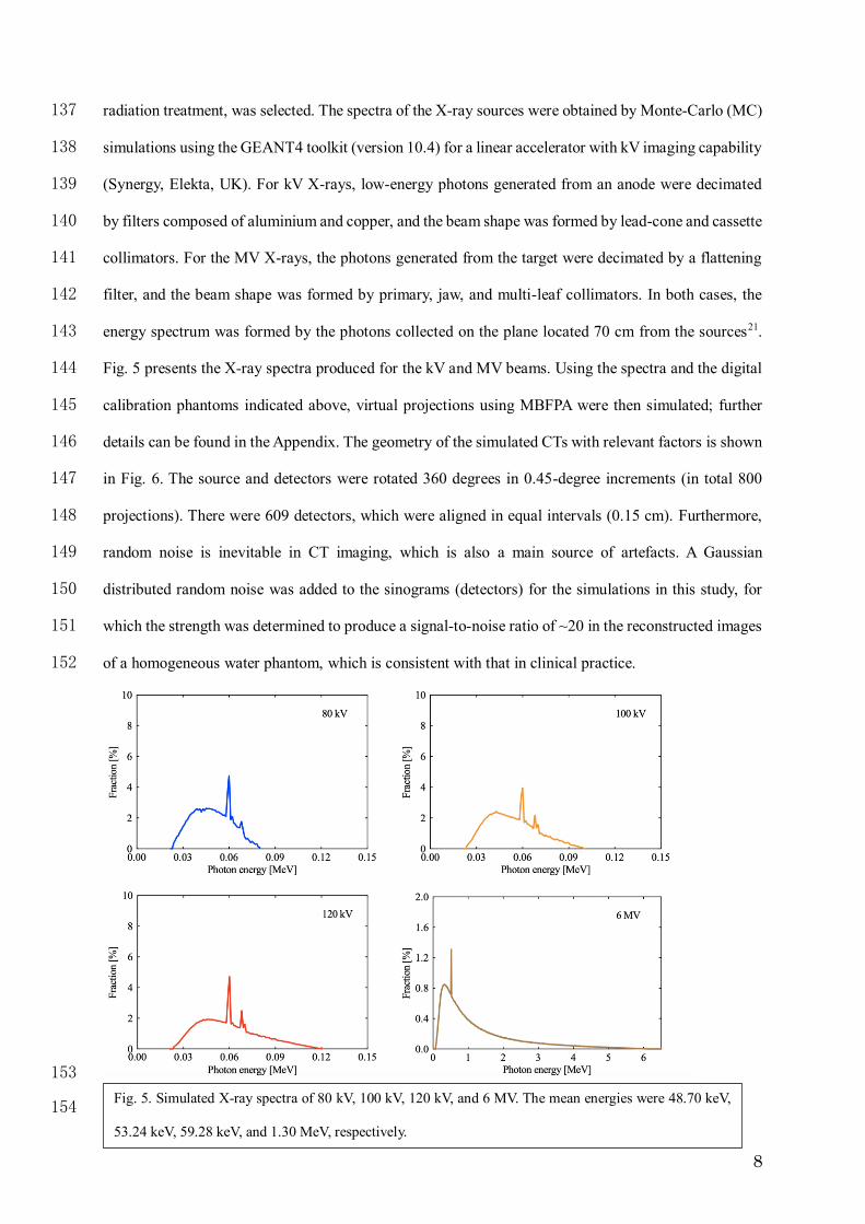
Fig. 5 presents the X-ray spectra produced for the kV and MV beams. Using the spectra and the digital 144

calibration phantoms indicated above, virtual projections using MBFPA were then simulated; further 145

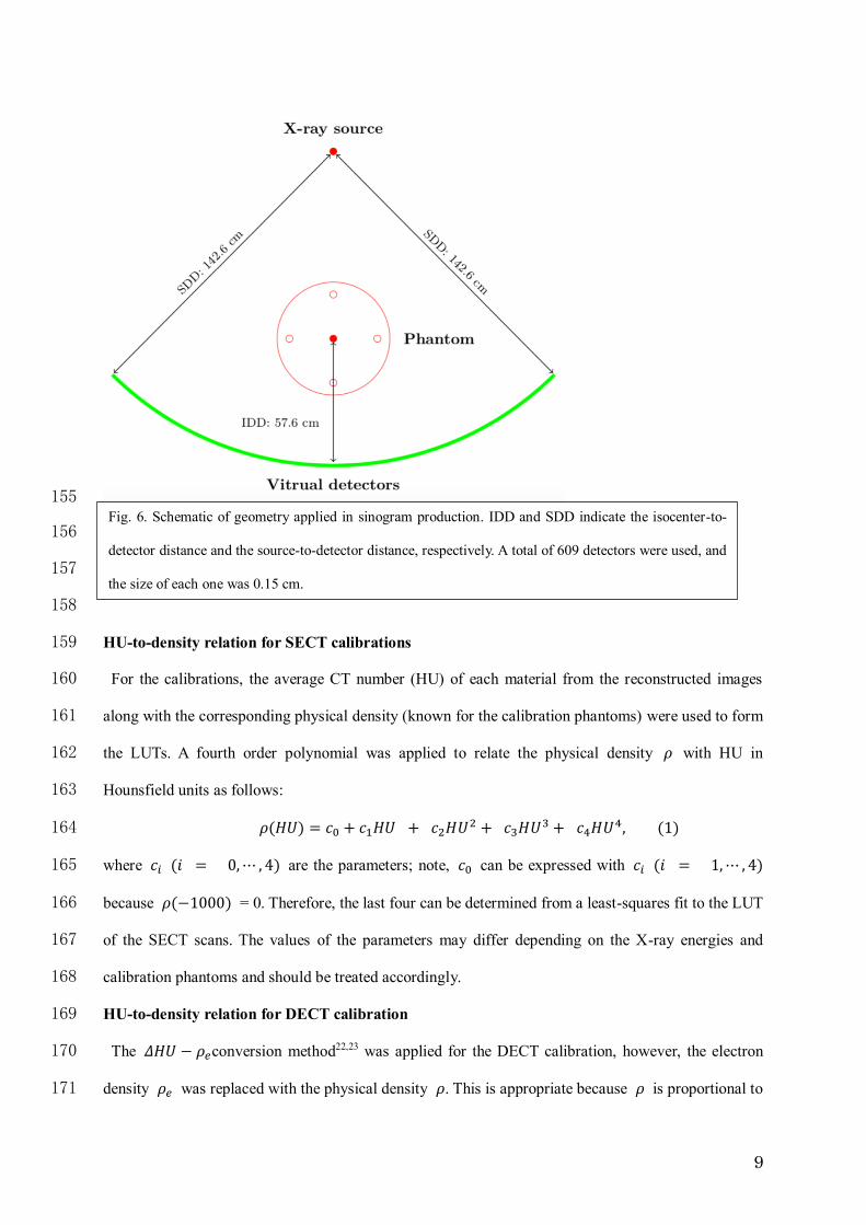
details can be found in the Appendix. The geometry of the simulated CTs with relevant factors is shown 146

in Fig. 6. The source and detectors were rotated 360 degrees in 0.45-degree increments (in total 800 147

projections). There were 609 detectors, which were aligned in equal intervals (0.15 cm). Furthermore, 148

random noise is inevitable in CT imaging, which is also a main source of artefacts. A Gaussian 149

distributed random noise was added to the sinograms (detectors) for the simulations in this study, for 150

which the strength was determined to produce a signal-to-noise ratio of ~20 in the reconstructed images 151

of a homogeneous water phantom, which is consistent with that in clinical practice. 152

153

154 Fig. 5. Simulated X-ray spectra of 80 kV, 100 kV, 120 kV, and 6 MV. The mean energies were 48.70 keV,

53.24 keV, 59.28 keV, and 1.30 MeV, respectively.

9

155

156

157

158

HU-to-density relation for SECT calibrations 159

For the calibrations, the average CT number (HU) of each material from the reconstructed images 160

along with the corresponding physical density (known for the calibration phantoms) were used to form 161

the LUTs. A fourth order polynomial was applied to relate the physical density 𝜌 with HU in 162

Hounsfield units as follows: 163

𝜌(𝐻𝑈) = 𝑐0 + 𝑐1𝐻𝑈 + 𝑐2𝐻𝑈2 + 𝑐3𝐻𝑈3 + 𝑐4𝐻𝑈4, (1) 164

where 𝑐𝑖 (𝑖 = 0, ⋯ , 4) are the parameters; note, 𝑐0 can be expressed with 𝑐𝑖 (𝑖 = 1, ⋯ , 4) 165

because 𝜌(−1000) = 0. Therefore, the last four can be determined from a least-squares fit to the LUT 166

of the SECT scans. The values of the parameters may differ depending on the X-ray energies and 167

calibration phantoms and should be treated accordingly. 168

HU-to-density relation for DECT calibration 169

The 𝛥𝐻𝑈 − 𝜌𝑒conversion method22,23 was applied for the DECT calibration, however, the electron 170

density 𝜌𝑒 was replaced with the physical density 𝜌. This is appropriate because 𝜌 is proportional to 171

Fig. 6. Schematic of geometry applied in sinogram production. IDD and SDD indicate the isocenter-to-

detector distance and the source-to-detector distance, respectively. A total of 609 detectors were used, and

the size of each one was 0.15 cm.

10

𝜌𝑒. The dual energy subtracted quantity 𝛥𝐻𝑈 was defined as follows: 172

𝛥𝐻𝑈 ≡ (1 + α)HU𝐻 − αHU𝐿 , (2) 173

where HU𝐻 and HU𝐿 denote the high-energy and low-energy CT numbers in Hounsfield units, 174

respectively. Further, α is a weighting factor for the subtraction, which is regarded as material-175

independent. Similar to a previous study22, the relation between 𝛥𝐻𝑈 and 𝜌 was assumed to be linear 176

for materials with low effective atomic numbers as follows: 177

𝜌(𝛥𝐻𝑈) = 𝑎𝛥𝐻𝑈

1000+ 𝑏 , (3) 178

where 𝑎, 𝑏, and α can be determined by a least squares fit to (HU𝐻 , HU𝐿) − 𝜌 data obtained from 179

DECT scans of materials with a known density 𝜌 in calibration phantoms, which is similar to the SECT 180

calibration. 181

Validation 182

The minimum 𝜒2 value of the fitting curves for the physical density were evaluated for all three 183

calibration phantoms. A total of 30 virtual images based on the ICRP110 human phantoms (shown in 184

Table I and Figs. 3 and 4) were independently prepared via virtual projections and image reconstructions. 185

The physical density distribution converted by the LUTs of each energy spectrum and calibration 186

phantom were compared with the ground truth. Statistical analysis was performed to determine the 187

differences in the RMSE among the chosen energies (for SECT), their combinations (for DECT), or the 188

chosen calibration phantoms. In particular, the following differences were assessed: 1) between SECT 189

and DECT, 2) between TS and BT(B), and 3) among the energies with BT(A) and BT(B). For the 190

statistical analysis, a Student's t-test was employed for the first two cases, while Tukey's range test was 191

employed for the last. 192

Results 193

Generated sinograms and reconstructed images 194

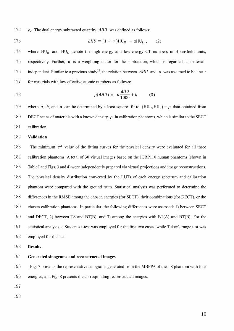
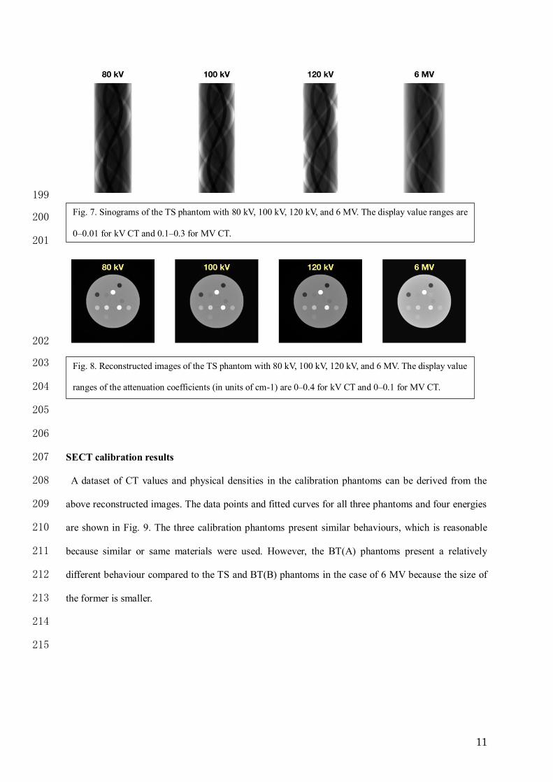
Fig. 7 presents the representative sinograms generated from the MBFPA of the TS phantom with four 195

energies, and Fig. 8 presents the corresponding reconstructed images. 196

197

198

11

199

200

201

202

203

204

205

206

SECT calibration results 207

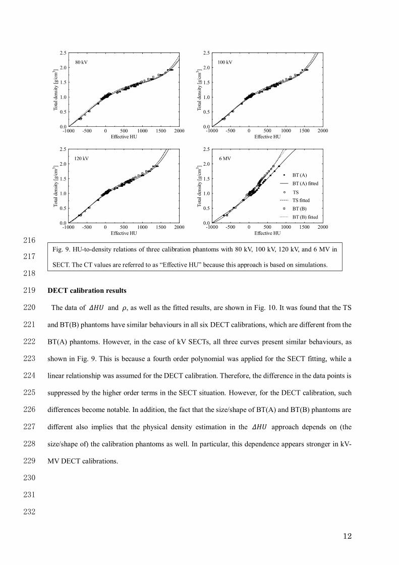
A dataset of CT values and physical densities in the calibration phantoms can be derived from the 208

above reconstructed images. The data points and fitted curves for all three phantoms and four energies 209

are shown in Fig. 9. The three calibration phantoms present similar behaviours, which is reasonable 210

because similar or same materials were used. However, the BT(A) phantoms present a relatively 211

different behaviour compared to the TS and BT(B) phantoms in the case of 6 MV because the size of 212

the former is smaller. 213

214

215

Fig. 7. Sinograms of the TS phantom with 80 kV, 100 kV, 120 kV, and 6 MV. The display value ranges are

0–0.01 for kV CT and 0.1–0.3 for MV CT.

Fig. 8. Reconstructed images of the TS phantom with 80 kV, 100 kV, 120 kV, and 6 MV. The display value

ranges of the attenuation coefficients (in units of cm-1) are 0–0.4 for kV CT and 0–0.1 for MV CT.

12

216

217

218

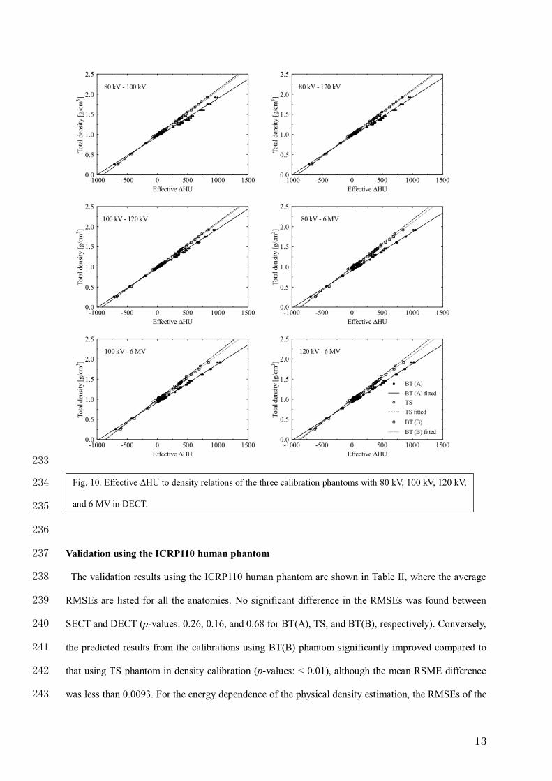
DECT calibration results 219

The data of 𝛥𝐻𝑈 and 𝜌, as well as the fitted results, are shown in Fig. 10. It was found that the TS 220

and BT(B) phantoms have similar behaviours in all six DECT calibrations, which are different from the 221

BT(A) phantoms. However, in the case of kV SECTs, all three curves present similar behaviours, as 222

shown in Fig. 9. This is because a fourth order polynomial was applied for the SECT fitting, while a 223

linear relationship was assumed for the DECT calibration. Therefore, the difference in the data points is 224

suppressed by the higher order terms in the SECT situation. However, for the DECT calibration, such 225

differences become notable. In addition, the fact that the size/shape of BT(A) and BT(B) phantoms are 226

different also implies that the physical density estimation in the 𝛥𝐻𝑈 approach depends on (the 227

size/shape of) the calibration phantoms as well. In particular, this dependence appears stronger in kV-228

MV DECT calibrations. 229

230

231

232

Fig. 9. HU-to-density relations of three calibration phantoms with 80 kV, 100 kV, 120 kV, and 6 MV in

SECT. The CT values are referred to as “Effective HU” because this approach is based on simulations.

13

233

234

235

236

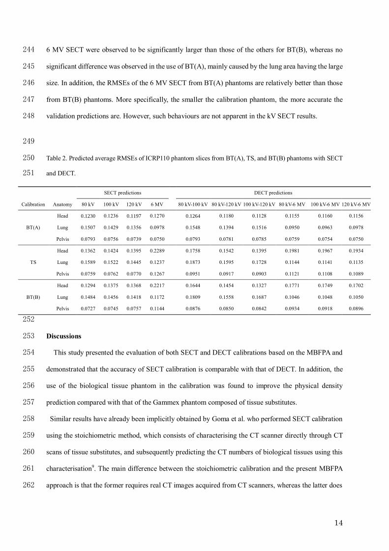
Validation using the ICRP110 human phantom 237

The validation results using the ICRP110 human phantom are shown in Table II, where the average 238

RMSEs are listed for all the anatomies. No significant difference in the RMSEs was found between 239

SECT and DECT (p-values: 0.26, 0.16, and 0.68 for BT(A), TS, and BT(B), respectively). Conversely, 240

the predicted results from the calibrations using BT(B) phantom significantly improved compared to 241

that using TS phantom in density calibration (p-values: < 0.01), although the mean RSME difference 242

was less than 0.0093. For the energy dependence of the physical density estimation, the RMSEs of the 243

Fig. 10. Effective ∆HU to density relations of the three calibration phantoms with 80 kV, 100 kV, 120 kV,

and 6 MV in DECT.

14

6 MV SECT were observed to be significantly larger than those of the others for BT(B), whereas no 244

significant difference was observed in the use of BT(A), mainly caused by the lung area having the large 245

size. In addition, the RMSEs of the 6 MV SECT from BT(A) phantoms are relatively better than those 246

from BT(B) phantoms. More specifically, the smaller the calibration phantom, the more accurate the 247

validation predictions are. However, such behaviours are not apparent in the kV SECT results. 248

249

Table 2. Predicted average RMSEs of ICRP110 phantom slices from BT(A), TS, and BT(B) phantoms with SECT 250

and DECT. 251

252

Discussions 253

This study presented the evaluation of both SECT and DECT calibrations based on the MBFPA and 254

demonstrated that the accuracy of SECT calibration is comparable with that of DECT. In addition, the 255

use of the biological tissue phantom in the calibration was found to improve the physical density 256

prediction compared with that of the Gammex phantom composed of tissue substitutes. 257

Similar results have already been implicitly obtained by Goma et al. who performed SECT calibration 258

using the stoichiometric method, which consists of characterising the CT scanner directly through CT 259

scans of tissue substitutes, and subsequently predicting the CT numbers of biological tissues using this 260

characterisation9. The main difference between the stoichiometric calibration and the present MBFPA 261

approach is that the former requires real CT images acquired from CT scanners, whereas the latter does 262

SECT predictions DECT predictions

Calibration Anatomy 80 kV 100 kV 120 kV 6 MV 80 kV-100 kV 80 kV-120 kV 100 kV-120 kV 80 kV-6 MV 100 kV-6 MV 120 kV-6 MV

BT(A)

Head 0.1230 0.1236 0.1197 0.1270 0.1264 0.1180 0.1128 0.1155 0.1160 0.1156

Lung 0.1507 0.1429 0.1356 0.0978 0.1548 0.1394 0.1516 0.0950 0.0963 0.0978

Pelvis 0.0793 0.0756 0.0739 0.0750 0.0793 0.0781 0.0785 0.0759 0.0754 0.0750

TS

Head 0.1362 0.1424 0.1395 0.2289 0.1758 0.1542 0.1395 0.1981 0.1967 0.1934

Lung 0.1589 0.1522 0.1445 0.1237 0.1873 0.1595 0.1728 0.1144 0.1141 0.1135

Pelvis 0.0759 0.0762 0.0770 0.1267 0.0951 0.0917 0.0903 0.1121 0.1108 0.1089

BT(B)

Head 0.1294 0.1375 0.1368 0.2217 0.1644 0.1454 0.1327 0.1771 0.1749 0.1702

Lung 0.1484 0.1456 0.1418 0.1172 0.1809 0.1558 0.1687 0.1046 0.1048 0.1050

Pelvis 0.0727 0.0745 0.0757 0.1144 0.0876 0.0850 0.0842 0.0934 0.0918 0.0896

15

not. In this study, the CT scanners were modelled, characterised by X-ray energy spectra directly, by 263

which various simulations, with not only the kV-range X-rays but also MV-range X-rays, could be 264

performed. Furthermore, the density results cannot be validated for real patients in the stoichiometric 265

calibration framework. However, using the proposed MBFPA-based calibration approach, the validation 266

is now possible by preparing, for example, the reconstructed CT datasets using the ICRP110 human 267

phantom, which could be considered as real patients to a certain extent. This study not only supported 268

the results of Goma et al. 9 but also newly presented that the tissue substitutes differ from the biological 269

tissues in physical density calibration. 270

The results of this study indicated that kV-MV DECT is not as outperformed as it was expected to be. 271

This is due to the large beam hardening effect in MV CT, compared to that in kV CT. This can be inferred 272

from the fact that different sizes of the calibration phantoms provided different calibration curves with 273

MV X-rays. For a more apparent indication, a simulation using monochromatic energy X-rays with 3 274

MeV was also performed, which does not suffer from beam hardening. In this case, no phantom size 275

dependence in the calibration curves was observed. The magnitude of beam hardening in MV CT could 276

also be observed in the homogeneous water phantom (of the same size as the TS phantom) by extracting 277

the reconstructed CT values in the centre and peripheral regions. Their relative difference was ~17% for 278

MV CT due to the cupping artefacts; however, this value is only ~10% for kV CT. Such ambiguity in 279

the MV CT with a practical spectrum significantly affected the accuracy of the calibration. Hence, DECT 280

with MV X-rays does not improve the accuracy of the physical density estimation as well as the SECT 281

of MV X-rays. Furthermore, the use of MV X-rays passing through a titanium filter could, to a certain 282

extent, reduce the beam-hardening effect. 283

Note that Yang et al. assessed the superiority of kV-MV DECT in determining proton stopping power 284

by generating 1 MV beams from MC calculations24. According to the authors, when CT number 285

uncertainties and artefacts such as imaging noise and beam hardening effects were considered, the kV-286

MV DECT improved the perfectly of SPR estimation substantially over kV-kV or MV-MV DECT methods. 287

The SPR estimation is directly influenced by the electron density (or physical density), and therefore, 288

Yang et al.’s study implied a substantial decrease in the physical density uncertainties in kV-MV DECT. 289

However, this study apparently supports the contrary. This might indicate that the beam hardening 290

16

effects were underestimated in MV CT in Yang et al.’s study because the authors assumed the “average 291

spectra” accurately modelled the CT scanner. Thus, the beam hardening effect should be carefully 292

treated in MV CT. 293

The proposed method can be considered an improvement over previous stoichiometric approaches in 294

which the parameters, depending on the X-ray spectrum, which characterise the CT scanner are 295

determined by fitting to the effective linear attenuation coefficients of a given material, whereas the 296

proposed method explicitly deals with the X-ray spectrum. Although the explicit handling of the X-ray 297

spectrum is advantageous in CT calibration, the requirement of the X-ray spectrum imposes limitations 298

for practical applications. That is, the exact energy spectrum of medical CT scanners is unknown, and 299

its direct measurement is difficult because of the high photon flux. Nevertheless, novel methods to 300

estimate X-ray spectra in practical CT scanners have been proposed in recent years25-27. Therefore, it is 301

reasonable to assume that X-ray spectra are currently available. 302

303

Conclusions 304

The proposed method using the MBFPA is useful in the theoretical analysis of physical density 305

calibrations. The accuracy of SECT calibration is comparable with that of DECT calibration and is 306

improved with the use of biological tissues. The size and shape of the calibration phantom could affect 307

the accuracy, especially for MV CT, mainly because of the beam hardening effects. The present method 308

based on the MBFPA can also be applied to various other studies, such as effective atomic number 309

estimations and material decompositions. 310

311

17

Declarations 312

Ethics approval and consent to participate 313

Not applicable. 314

Consent for publication 315

Not applicable. 316

Availability of data and materials 317

The datasets used and/or analysed during the current study are available from the corresponding author 318

upon reasonable request. 319

Competing interests 320

The authors declare that they have no competing interests. 321

Funding 322

This work was partially supported by JSPS KAKENHI (Grant No. 19K08201) and by the National 323

Natural Science Foundation of China (Grant No. 11735003). 324

Authors’ contributions 325

KL and DF conceived the idea. The method was discussed for KL, DF, and AH. Based on the discussion, 326

KL and AH developed the software, and KL and DF analysed the generated data. KL, AH, HL, and LG 327

presented the obtained results. KL and AH drafted the manuscript. All authors read, modified, and 328

approved the manuscript. 329

Acknowledgements 330

The authors thank Elekta for providing the structural information of the scanner heads for the MC 331

simulation of XVI systems. 332

333

18

Appendix: Material-based forward projection algorithm (MBFPA) 334

The material-based forward projection algorithm applied in the X-ray virtual projections is briefly 335

introduced here. According to Lambert-Beer's law, the photon number 𝑛𝑖 in the 𝑖 -th detector after 336

penetrating the object with attenuation coefficient 𝜇𝑗 in voxel 𝑗 is as follows: 337

𝑛𝑖(𝐸) = 𝑛0(𝐸)𝑒∑ −𝑎𝑖𝑗𝑗 𝜇𝑗(𝐸), (𝐴1) 338

where 𝐸 is the photon energy, 𝑛0 is the photon number in the X-ray source, and 𝑎𝑖𝑗 is the photon 339

pass length in voxel 𝑗, representing an element of the “system matrix”. If the spectrum of the X-ray is 340

considered (as bins), the total photon number in the 𝑖-th detector becomes the following: 341

𝑛𝑖𝑡𝑜𝑡𝑎𝑙 = ∑ 𝛼(𝐸)𝑛𝑖(𝐸)

𝐸

= ∑ 𝛼(𝐸)𝑛0(𝐸)

𝐸

𝑒∑ −𝑎𝑖𝑗𝑗 𝜇𝑗(𝐸), (𝐴2) 342

where 𝛼(𝐸) is the fraction of the corresponding photon energy bin. 𝜇𝑗(𝐸) is dependent on the atomic 343

number 𝑍 and the density 𝜌 of the materials in a voxel 𝑗 , which is expressed as a sum of the 344

attenuation coefficients for each element 𝑚 as follows: 345

𝜇𝑗(𝐸, 𝑍, 𝜌) = ∑ 𝑤𝑚𝜇𝑚,𝑗(𝐸, 𝑍, 𝜌)

𝑚

, (𝐴3) 346

where 𝑤𝑚 denotes the weight (fraction) of the 𝑚th element. For the energy range considered in this 347

study, the attenuation coefficient 𝜇𝑚,𝑗(𝐸, 𝑍, 𝜌) can be written as the sum of the processes of the 348

photoelectric effect, Compton scattering, and pair production as follows: 349

𝜇𝑚,𝑗(𝐸, 𝑍, 𝜌) = 𝜌𝑍𝑁𝐴

𝐴[𝜎𝑝𝑒(𝐸, 𝑍) + 𝜎𝑐𝑜𝑚𝑝(𝐸) + 𝜎𝑝𝑝(𝐸, 𝑍)], (𝐴4) 350

where 𝑁𝐴 and 𝐴 denote the Avogadro constant and atomic weight, respectively. 𝜎 is the cross section 351

of the photon – matter interactions. The cross section of the photoelectric effect can be approximated 352

by28 as follows: 353

𝜎𝑝𝑒(𝐸, 𝑍) = 3.45 × 10−6𝑟𝑒2(1 + 0.008𝑍)

𝑍3

𝐸3(1 −

𝐸𝑘

4𝐸−

𝐸𝑘2

1.21𝐸), (𝐴5) 354

where 𝑟𝑒 = 2.81794 fm is the classical electron radius and 𝐸𝑘 is the K-shell binding energy. The 355

latter is ignored in this study. The Compton scattering cross section is theoretically expressed by the 356

Klein–Nishina formula as follows: 357

19

𝜎𝑐𝑜𝑚𝑝(𝐸) = 2𝜋𝑟𝑒2 {

1 + 𝐸

𝐸2[2(1 + 𝐸)

1 + 2𝐸−

𝑙𝑛(1 + 2𝐸)

𝐸] +

𝑙𝑛(1 + 2𝐸)

2𝐸−

1 + 3𝐸

(1 + 2𝐸)2} . (𝐴6) 358

The cross section of the pair production is approximated as28 follows: 359

𝜎𝑝𝑝(𝐸, 𝑍) = 0.2545𝑟𝑒2(𝐸 − 2.332)

𝑍

137. (𝐴7) 360

As a result, the virtual projections were simulated by a ray-tracing method to generate sinograms. The 361

sinograms were simulated by considering the energy spectrum with a bin width of 1 keV in this study. 362

363

20

References 364

1. Mull RT. Mass estimates by computed tomography: physical density from CT numbers. Am J 365

Roentgenol 1984;143(5):1101-1104. 366

2. Langen KM, Meeks SL, Poole DO, Wagner TH, Willoughby TR, Kupelian PA, Ruchala KJ, 367

Haimerl J, Olivera GH. The use of megavoltage CT (MVCT) images for dose recomputations. 368

Phys Med Biol 2005;50(18):4259. 369

3. Yang Y, Schreibmann E, Li T, Wang C, Xing L. Evaluation of on-board kV cone beam CT 370

(CBCT)-based dose calculation. Phys Med Biol 2007;52(3):685. 371

4. Verhaegen F, Devic S. Sensitivity study for CT image use in Monte Carlo treatment planning. 372

Physics in Medicine & Biology, 50:937, 2005. 373

5. Fang R, Mazur T, Mutic S, Khan R, The impact of mass density variations on an electron Monte 374

Carlo algorithm for radiotherapy dose calculations. Phys Imag Radiat Oncol 2018;8:1. 375

6. Cozzi L, Fogliata A, Buffa F, Bieri S. Dosimetric impact of computed tomography calibration on 376

a commercial treatment planning system for external radiation therapy. Radiother Oncol 377

1998;48(3):335-338. 378

7. Schaffner B, Pedroni E. The precision of proton range calculations in proton radiotherapy 379

treatment planning: experimental verification of the relation between CT-HU and proton stopping 380

power. Phys Med Biol 1998;43(6):1579. 381

8. Schneider U, Pedroni E, Lomax A. The calibration of CT Hounsfield units for radiotherapy 382

treatment planning. Phys Med Biol 1996;41(1):111. 383

9. Gomá C, Almeida IP, Verhaegen F. Revisiting the single-energy CT calibration for proton therapy 384

treatment planning: a critical look at the stoichiometric method. Phys Med Biol 385

2018;63(23):235011. 386

10. Michalak G, Taasti V, Krauss B, Deisher A, Halaweish A, McCollough C. A comparison of 387

relative proton stopping power measurements across patient size using dual- and single-energy 388

CT. Acta Oncol 2017;56:1465-71. 389

21

11. Yang M, Virshup G, Clayton J, Zhu XR, Mohan R, Dong L. Theoretical variance analysis of 390

single-and dual-energy computed tomography methods for calculating proton stopping power 391

ratios of biological tissues. Phys Med Biol 2010;55(5):1343. 392

12. Hunemohr N, Paganetti H, Greilich S, Jakel O, Seco J. Tissue decomposition from dual energy ct 393

data for mc based dose calculation in particle therapy. Med Phys 2014;41(6Part1):061714. 394

13. II ICRU. Tissue substitutes in radiation dosimetry and measurement. International Commission on 395

Radiation Units and Measurements, 1989. 396

14. White DR, Woodard HQ, Hammond SM. Average soft-tissue and bone models for use in radiation 397

dosimetry. Brit J Radiol 1987;60(717):907-913. 398

15. Woodard HQ, White DR. The composition of body tissues. Brit J Radiol 1986;59(708):1209-399

1218. 400

16. Elbakri, IA, Fessler JA. Statistical image reconstruction for polyenergetic x-ray computed 401

tomography. IEEE Trans Med Imaging 2002;21(2):89-99. 402

17. Shen L, Xing Y. Multienergy CT acquisition and reconstruction with a stepped tube potential 403

scan. Med Phys 2015;42(1):282-296. 404

18. Ruchala KJ, Olivera GH, Schloesser EA, Mackie TR: Megavoltage CT on a tomotherapy system. 405

Phys Med Biol 1999;44:2597-2621. 406

19. Wertz H, Stsepankou D, Blessing M, Rossi M, Knox C, Brown K, Gros U, Boda-Heggemann J, 407

Walter C, Hesser C, Lohr F, Wenz F: Fast kilovoltage/megavoltage (kVMV) breathhold cone-408

beam CT for image-guided radiotherapy of lung cancer, Phys Med Biol 2010;55:4203-4217. 409

20. Pouliot J, Bani-Hashemi A, Chen J, et al. Low-dose megavoltage cone-beam CT for radiation 410

therapy. Int J Radiat Oncol Biol Phys 2005;61:552-560. 411

21. Sakata D, Haga A, Kida S, Imae T, Takenaka S, Nakagawa K. Effective atomic number 412

estimation using kV-MV dual-energy source in linac. Phys Medica, 2017;39:9-15. 413

22. Saito M. Potential of dual-energy subtraction for converting CT numbers to electron density based 414

on a single linear relationship. Med Phys 2012;39. 415

23. Tsukihara M, Noto Y, Sasamoto R, Hayakawa T, Saito M. Initial implementation of the 416

conversion from the energy-subtracted CT number to electron density in tissue inhomogeneity 417

22

corrections: An anthropomorphic phantom study of radiotherapy treatment planning. Med Phys 418

2015;42. 419

24. Yang M, Virshup G, Clayton J, Zhu XR, Mohan R, Dong L. Does kV–MV dual-energy computed 420

tomography have an advantage in determining proton stopping power ratios in patients? Phys Med 421

Biol 2011;56(14):4499. 422

25. Sidky EY, Yu L, Pan X, Zou Y, Vannier M. A robust method of x-ray source spectrum estimation 423

from transmission measurements: Demonstrated on computer simulated, scatter-free transmission 424

data. J Appl Phys 2005;97(12):124701. 425

26. Duan X, Wang J, Yu L, Leng S, McCollough CH. CT scanner x-ray spectrum estimation from 426

transmission measurements. Med Phys 2011;38(2):993-997. 427

27. Ha W, Sidky EY, Barber RF, Schmidt TG, Pan X. Estimating the spectrum in computed 428

tomography via Kullback–Leibler divergence constrained optimization. Med Phys 2019;46(1):81-429

92. 430

28. Yao W, Leszczynski KW. An analytical approach to estimating the first order x-ray scatter in 431

heterogeneous medium. Med Phys 200936(7):3145-3156. 432

433

434

435