SANDIA REPORT SAND2009-8377 Unlimited Release Printed December 2009 Power Electronics Reliability Analysis Mark A. Smith, Stanley Atcitty Prepared by Sandia National Laboratories Albuquerque, New Mexico 87185 and Livermore, California 94550 Sandia is a multiprogram laboratory operated by Sandia Corporation, a Lockheed Martin Company, for the United States Department of Energy’s National Nuclear Security Administration under Contract DE-AC04-94AL85000. Approved for public release; further dissemination unlimited.
Transcript
SANDIA REPORT SAND2009-8377 Unlimited Release Printed December 2009
Power Electronics Reliability Analysis Mark A. Smith, Stanley Atcitty Prepared by Sandia National Laboratories Albuquerque, New Mexico 87185 and Livermore, California 94550
Sandia is a multiprogram laboratory operated by Sandia Corporation, a Lockheed Martin Company, for the United States Department of Energy’s National Nuclear Security Administration under Contract DE-AC04-94AL85000.
Approved for public release; further dissemination unlimited.
2
Issued by Sandia National Laboratories, operated for the United States Department of Energy by Sandia Corporation. NOTICE: This report was prepared as an account of work sponsored by an agency of the United States Government. Neither the United States Government, nor any agency thereof, nor any of their employees, nor any of their contractors, subcontractors, or their employees, make any warranty, express or implied, or assume any legal liability or responsibility for the accuracy, completeness, or usefulness of any information, apparatus, product, or process disclosed, or represent that its use would not infringe privately owned rights. Reference herein to any specific commercial product, process, or service by trade name, trademark, manufacturer, or otherwise, does not necessarily constitute or imply its endorsement, recommendation, or favoring by the United States Government, any agency thereof, or any of their contractors or subcontractors. The views and opinions expressed herein do not necessarily state or reflect those of the United States Government, any agency thereof, or any of their contractors. Printed in the United States of America. This report has been reproduced directly from the best available copy. Available to DOE and DOE contractors from U.S. Department of Energy Office of Scientific and Technical Information P.O. Box 62 Oak Ridge, TN 37831 Telephone: (865) 576-8401 Facsimile: (865) 576-5728 E-Mail: [email protected] Online ordering: http://www.osti.gov/bridge Available to the public from U.S. Department of Commerce National Technical Information Service 5285 Port Royal Rd. Springfield, VA 22161 Telephone: (800) 553-6847 Facsimile: (703) 605-6900 E-Mail: [email protected] Online order: http://www.ntis.gov/help/ordermethods.asp?loc=7-4-0#online
3
SAND2009-8377 Unlimited Release
Printed December 2009
Power Electronics Reliability Analysis
Mark A. Smith Systems Readiness and Sustainment Technologies
Stanley Atcitty Energy Infrastructure and Distributed Energy Resources
Sandia National Laboratories P.O. Box 5800
Albuquerque, New Mexico 87185-MS1188
Abstract
This report provides the DOE and industry with a general process for analyzing power electronics reliability. The analysis can help with understanding the main causes of failures, downtime, and cost and how to reduce them. One approach is to collect field maintenance data and use it directly to calculate reliability metrics related to each cause. Another approach is to model the functional structure of the equipment using a fault tree to derive system reliability from component reliability. Analysis of a fictitious device demonstrates the latter process. Optimization can use the resulting baseline model to decide how to improve reliability and/or lower costs. It is recommended that both electric utilities and equipment manufacturers make provisions to collect and share data in order to lay the groundwork for improving reliability into the future. Reliability analysis helps guide reliability improvements in hardware and software technology including condition monitoring and prognostics and health management.
4
ACKNOWLEDGMENTS
This work has been sponsored by the United States Department of Energy (DOE) Office of Electricity Delivery & Energy Reliability under contract to Sandia National Laboratories (SNL). The authors would like to thank Gil Bindewald of DOE for giving us the opportunity to pursue this work. The project could not have happened without the cooperation of Harshad Mehta and Mahesh Gandhi of Silicon Power Corporation (SPCO) in providing a real-world power electronics project to address. They along with Bruce Thompson and Valerie Peters are responsible for successfully negotiating the project and getting it going. Dennis Longsine provided a detailed review and improvements to the final draft of the manuscript. Special thanks go to Simon Bird and other staff of SPCO for gathering data and answering our questions.
2. Terminology and Tools ............................................................................................................. 10 2.1. Equipment and Components ............................................................................................ 10 2.2. Failure .............................................................................................................................. 10 2.3. Fault Trees ....................................................................................................................... 10 2.4. Series and Parallel ............................................................................................................ 11 2.5. Downtime ......................................................................................................................... 11 2.6. Repairable and Non-repairable Systems .......................................................................... 11 2.7. Mean Time Between Failures .......................................................................................... 11 2.8. Reliability and Availability .............................................................................................. 11 2.9. Reliability Block Diagrams.............................................................................................. 12 2.10. Reliability Software ....................................................................................................... 12
3. Field Maintenance Data and Analysis ...................................................................................... 13 3.1. Collecting Field Maintenance Data ................................................................................. 13 3.2. Analyzing Field Maintenance Data ................................................................................. 14 3.3. Summary Data ................................................................................................................. 14
4. Fault Tree Analysis ................................................................................................................... 15 4.1. Collecting Reliability Design Information ....................................................................... 15 4.2. Creating a Fault Tree ....................................................................................................... 16 4.3. Analyzing a Fault Tree ..................................................................................................... 17
4.3.1. Series Fault Trees ............................................................................................... 17 4.3.2. Constant Failure Rate Approximation ................................................................ 17 4.3.3. Mean Time Between Failures ............................................................................. 18 4.3.4. Average Downtime ............................................................................................. 18 4.3.5. Availability ......................................................................................................... 18 4.3.6. Average Cost per Failure .................................................................................... 18 4.3.7. MTBF Sensitivity ............................................................................................... 18 4.3.8. Average Downtime Sensitivity and Availability Sensitivity ............................. 19 4.3.9. Cost Sensitivity ................................................................................................... 19
4.4. Other Analyses ................................................................................................................. 19 4.5. Application to Power Electronics .................................................................................... 20
5. Illustrative Example .................................................................................................................. 21 5.1. Specification, Application, and Failure of the S7 ............................................................ 21 5.2. Functional Breakdown and Fault Tree of the S7 ............................................................. 21 5.3. Analysis of the S7 ............................................................................................................ 21
6. Optimization ............................................................................................................................. 24 6.1. Optimization in General ................................................................................................... 24 6.2. Application to the S7 ....................................................................................................... 24
6
7. Prognostics and Health Management ........................................................................................ 27 7.1. Failure Detection Strategies ............................................................................................. 27 7.2. Maintenance Strategies .................................................................................................... 28 7.3. Health Management ......................................................................................................... 28 7.4. Risk-Based Cost Optimization ......................................................................................... 28
Distribution ................................................................................................................................... 33
LIST OF FIGURES Figure 2-1. An example of a fault tree. ........................................................................................ 10 Figure 2-2. An example of a reliability block diagram. ............................................................... 12 Figure 5-1. A fault tree for the Solid-State Shunt SubStation Sag Suppressor. ........................... 21 Figure 5-2. Relative contributions to MTBF from each primary failure mode. .......................... 22 Figure 5-3. Relative contributions to Downtime/Availability from each primary failure mode. 23 Figure 6-1. Evolution of the fitness objective function over 29 generations. .............................. 25 Figure 6-2. Maximizing the MTBF objective. ............................................................................. 25 Figure 6-3. Satisfying the total component MTBF constraint. .................................................... 26 Figure 7-1. Probability of non-detection as a function of failure prediction lead time. .............. 29
LIST OF TABLES Table 5-1. Basic reliability metrics for the S7. ............................................................................ 22 Table 7-1. Failure detection strategy dependencies. .................................................................... 27 Table 7-2. Maintenance strategy dependencies. .......................................................................... 28
7
PREFACE This report is the final, main deliverable of the Power Electronics Reliability Project under the Energy Storage Systems Research Program at Sandia National Laboratories (SNL or Sandia) funded by the Power Electronics Program of the U.S. Department Of Energy (DOE/PE) Office of Electricity Delivery and Energy Reliability (http://www.oe.energy.gov/). It gives reliability data collection recommendations and describes a general process for analyzing the reliability of any power electronics (PE) system. The overall goal of this project has been to utilize Sandia’s modeling, simulation, and optimization capabilities to address DOE objectives in enhancing the reliability and availability of PE [1]. The modeling and analysis process described here is an adaptation of Sandia’s reliability analysis methodology developed by the Systems Readiness and Sustainment Technologies department. In addition to the general technological capabilities mentioned above, Sandia has developed specific software tools for (1) Design for Reliability/Maintainability, (2) Systems of Systems Analysis, (3) Integrated Logistics Support, and (4) Technology Management Optimization. These tools and technologies have been developed and validated through use with a range of military and industrial customers. To further extend such capabilities while helping the PE industry, another goal of the project has been to apply the reliability analysis methodology to a specific PE application. Accordingly, this adaptation of Sandia’s process has benefitted greatly from an engagement with Silicon Power Corporation (SPCO) to model and analyze the reliability of their Solid-State Current Limiter (SSCL). Further goals in that instance have been to:
1. Use SPCO expert knowledge to create a system reliability model of the SSCL. 2. Analyze the model to anticipate reliability issues and suggest reliability improvements in
components, software, and operations. 3. Use optimization to explore opportunities for Prognostics and Health Management
(PHM). While no specific design or reliability details are given, lessons learned from that engagement have been incorporated throughout the text. This particular work—from the perspective of a manufacturer of PE equipment—has focused on reliability analysis at the level of systems containing high-powered semiconductor switches such as might be found in an electrical switching station, substation, or converter station. However, with the right partnerships, these technologies, tools, and processes could be adapted—or new ones developed—to address reliability for smaller or larger PE systems; specifically, devices or transmission and distribution networks. Research into PE applications of condition monitoring (CM), prognostics, or health management (HM) could also be undertaken.
8
ABBREVIATIONS AAC Average Annual Cost ADT Average Annual Downtime CM Condition Monitoring CPF Cost per Failure DOE Department of Energy GA Genetic Algorithm HM Health Management IGBT Insulated Gate Bipolar Transistor MTBF Mean Time Between Failures MTTR Mean Time To Repair PE Power Electronics PHM Prognostics and Health Management RBD Reliability Block Diagram SCADA Supervisory Control and Data Acquisition SF Sensitivity Factor SPCO Silicon Power Corporation SSCL Solid-State Current Limiter
9
1. INTRODUCTION This report provides the DOE and industry with a general process for analyzing the reliability of any power electronics (PE) system. The analysis proceeds by reducing field maintenance data or creating a model of equipment failure that logically traces back to the reliability of individual components. The intent is to enable engineers involved in PE to perform basic reliability analysis on their own systems and, along with management, start to build an internal reliability program which is incorporated into their work. The reliability analysis process can:
1. Encourage stakeholders to think in concrete terms about reliability and associated costs and how they can be understood and managed.
2. Provide information about how system design and reliability at the component level affect overall reliability.
3. Help identify components that may need additional testing or more rigorous quality assurance scrutiny.
4. Show where redundancy helps and where it adds little value. 5. Show how operational changes and maintenance policies can affect system reliability. 6. Help managers make near-optimal choices with regards to upgrades. 7. Illuminate further pathways to improving PE reliability.
The rest of the report is organized as follows. Section 2 introduces some important terminology and analysis tools that will be used thereafter. Section 3 discusses the first approach to reliability analysis which is to collect field maintenance data and reduce it to derive conclusions. Section 4 is the core of the report and discusses a second approach to reliability analysis based on fault trees and summary failure data for components. Fault trees confer the advantage of being able to analyze redundancy while the use of summary data derived from subject matter expert opinion means the analysis can apply to systems that don’t yet exist. Some ways in which PE reliability analysis is different from reliability analysis for other systems are also given here. Section 5 presents an example of using fault tree analysis on a fictitious piece of PE equipment, the S7. Section 6 explains optimization in the context of reliability analysis and develops an example based on the S7. Section 7 introduces prognostics and health management (PHM) and how it can be informed by optimization analysis. Section 8 presents some recommendations to industry on data collection which is the key to improving reliability in the future. Finally, Section 9 concludes by expanding on the list of benefits above.
10
2. TERMINOLOGY AND TOOLS This section introduces some important concepts in reliability engineering and establishes terminology for PE that will be used throughout the rest of the report.
2.1. Equipment and Components Equipment (or the system) refers to related electrical boxes such as those which might be found in an electrical switching station or substation. Electrical and mechanical components are what the equipment is comprised of and include items such as capacitors, circuit boards, and cooling machinery as well as semiconductor devices. Component, part, and device are synonyms. Components do not include conditions, procedures, or elements—including humans—that are external to the system.
2.2. Failure A failure is an all-or-nothing event, meaning a component, the system, an operator, or the electrical grid, is not working as desired. Failure is a binary concept, not continuous one, and it does not describe partially failed components. A component or system either meets a certain specification or it doesn’t in which case it has failed. The costs or consequences of a failure are treated separately. Sometimes, certain types of failures such as scheduled maintenance, operator error, or environmental condition are given other names. For example, scheduled maintenance is usually called an “event” to distinguish it from unscheduled maintenance which stems from a component failure, but scheduled or unscheduled, the effects are similar since electrical transmission and distribution equipment is typically supposed to operate 24/7. Similarly, some distinguish between failures and faults where the word “fault” in this report should not be confused with the usual meaning of fault in the context of the electric power industry. To keep things simple, we will usually call all of these things failures. Failures that are not broken down into further causes will be called primary failures.
2.3. Fault Trees A fault tree is a graphical representation of a Boolean expression for the failure of a system in terms of the failures of its components (see Figure 2-1).
Figure 2-1. An example of a fault tree.
The entire system S fails if both components A and B fail or if component C fails. The fault tree is composed of AND gates and OR gates. If there is no redundancy in the system, the corresponding fault tree can be expressed entirely with OR gates. More complex situations (e.g., time ordering of failures) can be modeled by including specialized gate symbols.
11
2.4. Series and Parallel In reliability engineering, the terminology of series and parallel follow the analogy of a chain. A chain will fail if any of the links in series fail. However, if the links are in parallel, the chain will only fail if all of the links fail. Therefore, an OR gate represents failures that combine in series while an AND gate represents failures that combine in parallel. It is important to note that the structure of a fault tree matches the functional structure of a system; it does not necessarily match the electrical structure of the system. Components such as thyristors in electrical series may function in parallel for reliability purposes and vice versa.
2.5. Downtime Downtime usually refers to the period of time that a system is down and typically has a one-to-one connection with a failure. However, there can be downtime without any component failures, for example, in the case of preventative maintenance, testing, or inspection. Conversely, if there is redundancy for a component and the component can be repaired while the system continues to run, a failure may not cause any downtime. In this latter case, the time that an expeditious repair would take is considered to be the downtime.
2.6. Repairable and Non-repairable Systems Non-repairable systems are based on failure probabilities over a fixed period of time. In this case, the failure probabilities at the end of the time interval are combined by the fault tree by the usual laws of probability. One PE example where a non-repairable system model might be appropriate is that of a photovoltaic inverter system over the period of a single day from sunrise to sunset. Repairable systems operate indefinitely and are based on failure rates and repair times. Since PE systems involved in transmission and distribution are typically intended to operate 24/7, they are treated as repairable systems in this report. System failure rates and failure probabilities can be estimated from stationary solutions to continuous-time Markov processes.
2.7. Mean Time Between Failures The Mean Time Between Failures (MTBF) is the average length of time a system will run without failing. For a non-repairable system, it is the average time until the first failure. For a repairable system, it is the average time from the end of one downtime period to the beginning of the next.
2.8. Reliability and Availability Reliability is the probability that a system will not fail in the timeframe of interest under given conditions. For a repairable system with a constant failure rate, the reliability or survival function is
/MTBF. In the case of 24/7 operations, availability is the fraction of the time that a repairable system is working. Of course, it is complementary to the fraction of the time that the system is down.
12
2.9. Reliability Block Diagrams A reliability block diagram (RBD) focuses on the reliability of components rather than failures. If a component fails, it cuts the diagram at that point. The system works if there is an unbroken path from the beginning of the diagram to the end. The RBD in Figure 2-2 corresponds to the fault tree in Figure 2-1.
Figure 2-2. An example of a reliability block diagram.
The system S works if component A or B work and if component C works. As with fault trees, more complex situations can be modeled by including specialized fault-tree-like symbols. RBDs tend to be more popular than fault trees in commercial reliability software although it is perhaps easier to express complex forms of redundancy using fault trees.
2.10. Reliability Software The right software tools can help greatly with the reliability modeling and analysis tasks described in this report. There are any number of commercially available software packages that can do various types of analyses described herein, although it is not the purpose of this report to recommend or teach any particular one. Many of the analyses can even be done with spreadsheets. Numerical, mathematical, or statistical programs may also prove useful depending on what the analyst is used to. Of course, general-purpose programming language software can also be used in cases where iteration would be useful. Sandia has developed its own program called Pro-Opta [2, 3, 4] which has been used to do all of the analyses described below. Pro-Opta contains analytic approximations for reliability metrics based on fault trees which make it fast and suitable for performing optimization studies [5].
13
3. FIELD MAINTENANCE DATA AND ANALYSIS There are two main approaches to performing reliability analysis of PE equipment. The first approach is to collect and analyze maintenance data from fielded systems. This type of analysis does not necessarily require any knowledge of the internal workings of the equipment, but detailed analysis of the data can provide useful insights. The second approach is to create a model of the logical connection between failures of the overall system and failures of the individual components whose reliability can be characterized. The first approach is viable only when one already has equipment deployed while the second can also be performed even before the equipment is built. Since the future electric grid will be enabled by new PE equipment just now under development, the main focus of this report will be on the latter, systems-modeling approach. As described subsequently in Section 4, fault trees will be used to model the equipment while failure rates and downtimes will describe the reliability of the components. However, it is worth briefly looking and the field data analysis approach in this section. The field data analysis approach can be used to answer questions such as: Which failures are causing the most reliability problems? Which failures are costing the most? Which pieces of equipment are causing the most problems? When are most of the failures occurring? How much would the system reliability improve if a certain component never failed? The field data analysis can also be followed by optimization studies to answer questions such as: What inventory of spare parts should be on hand to minimize maintenance costs? Given a certain budget and options for upgrading components, what is the maximum reliability that can be achieved?
3.1. Collecting Field Maintenance Data The field maintenance data basically consists of a list of maintenance records. This list might be stored in a table in a (temporal) relational database along with other tables that define codes or record other events. In general, there is a many-to-many relationship between failures and maintenance actions, and it can get quite complicated, especially for a system that does not have to operate 24/7. However, we will simplify by assuming it is possible to recast the records into a one-to-one mapping between a component (i.e., every failure must be attributed to a single component) and a maintenance action (which translates into a certain amount of downtime). Then the basic information that needs to be recorded for each failure is as follows:
1. Date and time 2. Equipment ID 3. Failure Mode ID (this must be the same across all occurrences and all equipment for
modes that are to be considered the same and different for modes that are to be considered different)
4. Downtime 5. Repair cost
Some of this information can be further broken down depending on what questions are to be addressed. Downtime can be broken into administration time, waiting time, and actual
14
maintenance time. Cost can be broken down into labor time costs, part costs, and fixed costs. Other meaningful details could be added to each record including:
a. A functional breakdown of the component involved. b. A user-friendly textual description of the failure mode (ideally, this will always be the
same for the same failure mode at different times or on different equipment). c. The type of failure (component failure, preventative maintenance, human error,
inspection). d. A description of the failure mechanism (fail open, fail closed) e. Maintenance action required (replacement, repair, adjustment). f. Downstream consequences of the failure. g. The level of system degradation if there is redundancy.
Of course, the more detail desired, the more difficult the data collection will be. Since certain data may be missing or invalid, the records must be cleaned, and any assumptions used to do so should be made explicit. For example, the labor cost may not be captured in the maintenance log, so it could be split in proportion to some standard “book rate” repair time.
3.2. Analyzing Field Maintenance Data This type of analysis implicitly assumes a series model which is to say there is no redundancy, and every failure causes downtime. The main reliability metrics of interest are MTBF, availability, downtime (per failure or per year), and cost (per failure or per year). It is straightforward to calculate these metrics once the data is in the right form. They can be calculated for all the data, or they can be partitioned and averaged the by groups of equipment, groups of failure modes, failure types, subsystems involved, or time period. The more detail captured in the maintenance records, the more ways the analysis can be broken down. Other quantities of interest are sensitivities and variabilities in the above metrics with respect to each failure mode. They can be normalized and plotted together as a Pareto chart from greatest to least which quickly shows which failure modes contribute the most to that metric. Sensitivity refers to the fraction of each quantity that is determined by a given failure mode. Variability refers to differences in the metrics between copies of the same type of equipment. It can be used to identify equipment that is having more problems than most.
3.3. Summary Data In addition to obtaining equipment-level metrics, the field data for each component or external failure type can be summarized to create or augment a “failure mode library.” Such a library contains data on failure rates and downtimes for various failure modes. The failure rate data could also come from laboratory tests on individual components, supplier information, historical data on similar devices, or subject matter expert opinion. Combining all sources of failure data provides the most complete picture of the properties of each failure mode. Downtimes rely heavily on operational specifics, but they can also be estimated. Similarly, cost data may also be estimated or introduced later. Summary data can be used in fault tree analysis as described next.
15
4. FAULT TREE ANALYSIS As an alternative to field data analysis as described previously in Section 3, fault tree analysis is a systems approach to performing reliability analysis of PE equipment and is the main focus of this report. The main difference between the two approaches is that field data analysis requires failure data from extant installations whereas fault tree analysis does not. Another major difference is that fault trees can analyze the effects of redundancy and the extent to which it helps, which is essential to investigate alternative designs. In other words, fault tree analysis allows reliability issues to be uncovered and addressed before they become a problem. Otherwise, both approaches yield a model of system failure: in the former case, the field data is summarized into a statistical model whereas in the latter case, the fault tree constitutes the model. If the failure mode parameters are included in the fault tree model, both models can answer similar questions and can both be used for “what-if” analysis and optimization studies. The PE reliability analysis process starts with collecting information necessary to create a system reliability model in the form of a fault tree. The tree traces the logical connection between primary failures and system failures while taking redundancy into account. Data on the primary failure modes will come in the form of summary data as described in the previous section. As with the field data collection and analysis approach, it is important to make explicit any assumptions about the data or the structure of the model.
4.1. Collecting Reliability Design Information To perform a good reliability analysis on a piece of PE equipment using a systems-modeling approach, a great deal of information and expertise is needed. Furthermore, the modeling and analysis process tends to be iterative, so it is best to do it in a team environment rather than attempt to transfer all the information to a single analyst. While not all of the following information must be provided explicitly, the modeling and analysis will tacitly assume something for each element (depending on the questions the analysis is designed to answer), so there is substantial room for error if the corresponding knowledge is not captured by the team.
1. Information on the design, function, and principles of operation of the equipment. Design information includes schematics and mechanical drawings. Function information says what the equipment is supposed to do under various circumstances. Principles of operation refer to the underlying physics of how the device works and therefore what can go wrong. This information will determine how failure modes combine to cause a system failure or how the components work to avoid it. Experts will be needed to decide on the system failure of interest.
2. Specifications and application notes. The specifications will be used to define a level of performance which defines failure, and the application notes will provide the context in which the equipment will be deployed including the frequency and severity of external failures. This information will also be used to determine the consequences of various system failures. Input from electric utilities that will use the equipment is very valuable here.
16
3. Data is on the primary failure modes: specifically, the failure rate of each one. It could take the form of raw data or data that has already been summarized. Each failure mode should be uniquely labeled, and can be further described by any of the details listed in Section 3.1, a–g.
4. Information on operations and maintenance. It will include information on equipment utilization levels (when the equipment is used and under what conditions). Most importantly, it will include downtimes and costs associated with maintenance. The repair time is commonly referred to as downtime, but they are potentially different if repairs can be performed on redundant components while the system is up. This is also where the human element enters the equation: actions that could lead to equipment failure may be listed as primary failures.
In all the areas above, the lack of concrete data need not stop the modeling process because there is always some information, knowledge, or experience available to support assumptions and estimates. If acceptable to the stakeholders, team members can make and document assumptions and press on.
4.2. Creating a Fault Tree A fault tree is a model of reliability that reflects the functional structure of the PE equipment. Creating a fault tree is the analytical process at the core of this report and must be done with care. The team must first decide on an unambiguous definition of system failure. Primary failure modes may have already been identified with the belief that they would be important, but they do not necessarily contribute to that particular defined system failure. Start building the fault tree at the root which corresponds to the defined system failure of interest. If any failure is not a primary failure, break it into failures that are immediate causes of that failure as follows. Look for the all of the smallest possible groups of immediate causes that can cause the failure. Those causes will themselves be failures. All of the failures within each group should be combined with an AND gate to create intermediate failures. All of the intermediate failures are in turn combined with an OR gate to give the root failure. Note that any given failure may feed into more than one gate. The tree is further developed by repeatedly breaking down each intermediate failure in a similar fashion until only primary failures remain. The tree can be simplified at any point in the development using the rules of Boolean algebra. Keep in mind that in our terminology, primary failures can even include things like scheduled maintenance, operator errors, and drops in grid power quality. Primary failures that cannot contribute to the defined system failure should not end up on the tree. At this point, the tree is only making a static statement about what sets of primary failures together imply that the equipment will be in a failed state. There is no implication of simulated time. However, the notion of time could start coming in by further labeling gates to indicate the order in which failures must happen; for example, one component may be unused until another one fails. Ways to analyze the resulting tree to derive reliability metrics will be discussed next.
17
4.3. Analyzing a Fault Tree Given a fault tree, supporting failure mode summary data, and operational information, one would like to calculate a number of metrics to assess reliability and use the results for decision purposes. There are different ways to approximate the calculations, and the answers depend on the particular problem formulation as well as assumptions on how failures and repairs dynamically unfold over time. Furthermore, if closed-form formulas are desired, certain mathematical approximations are usually required. If averages over sample histories are sufficient, direct Monte Carlo simulation can eliminate the approximations and accommodate a wider range of assumptions (although random errors will be introduced).
4.3.1. Series Fault Trees In many cases, a fault tree amounts to a series model: it only has OR gates. For a system with redundancy, the calculations are much more complicated because of the contribution of repairs performed during partially failed states. For example, for a series system, downtimes do not affect the system MTBF, but for a redundant system they do. Trees with redundancy can sometimes be approximated with series trees by replacing redundant sub-trees with nearly equivalent primary failures.
4.3.2. Constant Failure Rate Approximation When calculating reliability metrics, the way failures unfold over time depends on the failure distribution, but the failure distribution is not solely determined by the MTBF. Constant failure rates (denoted by λ) lead to exponential failure distributions:1
· However, components and systems frequently show wear-out effects which means that failure rates increase with time. Nevertheless, throughout this report, we will assume failure rates are constant so that λ 1/MTBF. There are a number of reasons to use a constant failure rate approximation for all failures in contrast to an increasing failure rate when analyzing a fault tree:
1. Tractability. Closed-form formulas for estimating reliability metrics are simpler and much easier to derive.
2. Conservative. For a brand new system, the MTBF will underestimate the time to first failure.
3. Correct in time. Even if the system MTBF underestimates the time to first failure, it will correctly describe the MTBF over an extended period of time (assuming components are not replaced before they fail).
4. Describing a fleet. The MTBF will correctly describe the MTBF of a fleet of many similar systems of varying ages (assuming components are not replaced before they fail).
5. Parameter estimation. Fitting a non-constant failure rate failure distribution would require even more data to estimate at least one more parameter beyond the MTBF.
6. End use. Regardless of early biases in MTBF, the sensitivity results will still trend in the right direction and the fault tree can be used for optimization, uncertainty analysis, or to identify problem areas.
1 Colloquially speaking. Technically speaking, this is a failure density function, and the integral of the density is the distribution.
18
Using “more correct” failure distributions such as lognormal or Weibull is likely to require Monte Carlo simulation where the lack of analytic formulas makes optimization much more difficult. Even those distributions don’t simultaneously include both wear-out effects and wear-in (“infant mortality”) effects. The sections below give formulas for metrics for repairable systems having series fault trees and constant primary failure rates. The failure rate, MTBF, Mean Time to Repair, and Cost Per Failure associated with component are denoted by λ , MTBF , MTTR , and CPF respectively. The formulas describe system behavior averaged over a long period of time so there is no notion of time left: they are steady-state results and don’t describe transients. The formulas are simple enough to calculate on a spreadsheet, and even with the caveats, they frequently provide useful results. If more detailed results are desired, more sophisticated methods and software will be required. Even then, it is useful to be able to compare the more detailed results with the results from simple formulas.
4.3.3. Mean Time Between Failures For a series system, failure rates add to give a total system failure rate: λ ∑ λ . Therefore, the MTBF of the entire system, not including downtime is
MTBF1
∑·
4.3.4. Average Downtime The average downtime per failure is the total downtime for each failure mode weighted by the fractional failure rate for that mode:
MTTR∑ MTTR
∑·
4.3.5. Availability Availability is a fraction which refers to the amount of time a system is running or available to run normalized by some total time of interest (e.g., working hours or desired operating hours). In the case of a system that is intended to run 24/7, it is
MTBF
MTBF MTTR
11 ∑ MTTR
·
4.3.6. Average Cost per Failure The average cost per failure is the total cost for each failure mode weighted by the fractional failure rate for that mode:
CPF∑ CPF
∑·
4.3.7. MTBF Sensitivity The MTBF sensitivity factor for failure mode gives the approximate fractional change in MTBF if failure mode were to never occur. It is defined as
SFMTBF
∑
19
which is the same as the fraction of the failure rate contributed by failure mode . Plotting these from highest to lowest gives a Pareto chart showing which failure modes are most important for driving MTBF. An example chart is given in Section 5.3.2.
4.3.8. Average Downtime Sensitivity and Availability Sensitivity The average annual downtime (ADT) sensitivity factor for failure mode is the relative reduction in the average downtime rate if failure mode were to never occur:
SFADTMTTR
∑ MTTR·
The availability sensitivity factor for failure mode is the relative reduction in unavailability if failure mode were to never occur, and is therefore exactly the same as ADT sensitivity. It has a different name because sometimes it is useful to think in terms of availability (or uptime) instead of downtime (or unavailability) even though the failures which affect them are the same in terms of their proportion of impact. Plotting these from highest to lowest gives a Pareto chart showing which failure modes are most important for driving downtime (or availability). An example chart is given in Section 5.3.3.
4.3.9. Cost Sensitivity The sensitivity factor to average annual cost (AAC) for failure mode is the relative reduction in the average cost rate if failure mode were to never occur:
SFAAC CPF
∑ CPF·
4.4. Other Analyses In addition to calculating reliability metrics for series systems, one would also like to be able to calculate them for redundant systems. For both types of systems, it might be further desirable to do uncertainty and/or optimization analysis. Such analyses can be done with Pro-Opta or other reliability software or with tools developed separately. The example in subsequent sections illustrates both redundancy and optimization analysis but not uncertainty analysis. Uncertainty analysis quantifies the impact of uncertainty in the input parameters on the uncertainty in output metrics. Uncertainty could describe machine-to-machine variability and/or a wide confidence interval for a given parameter. In the case of a fleet of machines, the goal would be to identify machines that have outlier metrics and may therefore be having particular problems. In the case of uncertainty in summary data, one would like to find out which uncertain parameters are important to the final results and therefore might be good places to focus further data collection efforts. In principle, uncertainty analysis is easy using a sampling approach: parameters are sampled from the appropriate distributions and the variation in output metrics is observed. Optimization analysis can be used to get the most out of a current or future system. Setting up an optimization problem consists of (1) defining an objective function to minimize or maximize, (2) listing available options along with their impact on the constraints and the failure mode data, and (3) defining constraints. An example would be to minimize downtime by selecting a spare parts inventory subject to a warehouse space constraint. Another example would be to maximize
20
MTBF by improving component reliability subject to a given budget for upgrades. In principle, the problem is easy to solve by simply trying every option and picking the best one that satisfies the constraints. In practice, there is a combinatorial explosion of options, and an optimization routine must be used to approximate the best solution. Having closed-form formulas for the reliability metrics is extremely useful in this regard because they are fast and deterministic to evaluate. Many optimization algorithms are available for solving the problem including conjugate gradient methods, simulated annealing, and genetic algorithms.
4.5. Application to Power Electronics At this point, it is useful to mention some of the ways in which PE presents special challenges for reliability analysis. Since PE equipment is an integral part of the power grid, it is difficult to draw a system boundary that contains all the potential causes of failure. Besides random internal failures, external causes of failure including human error, weather, and power events may be of greater interest than external causes in other domains. Closely related to the problem of system boundary is the question of defining what it means for the system to fail. Certainly it is a failure if the PE equipment doesn’t alleviate the power issue for which it was designed, but what if it is off-line when the power is otherwise fine? What if a failure inside the equipment causes some other problem for the grid? What if the equipment is in a degraded state where some of the redundant components have failed but the system still works? Since the system boundary may be defined in different ways and there may be various degraded states of interest, it is helpful to create several fault trees corresponding to different definitions of system failure. When it comes to using reliability analysis for making improvement recommendations, there are a number of issues. Every installation is likely to be unique, so utility input is needed even though it may be difficult for the PE manufacturer to obtain. In cases where power failures are a possibility, reliability is more important than availability because the grid is supposed to operate 24/7, and once there is a power failure, the consequences don’t depend very strongly on the length of the downtime. That makes analysis easier but it makes design or redesign for reliability more challenging. Finally, optimization analysis is clouded by the fact that costs to the utility and to society may not be borne by the manufacturer.
21
5. ILLUSTRATIVE EXAMPLE This example involves an imaginary device: the Solid-State Shunt SubStation Sag Suppressor or S7. It is not offered as a device that could really work with so few components but was contrived to have many features that will be familiar to PE engineers.
5.1. Specification, Application, and Failure of the S7 The S7 is to be installed in a substation in a shunt configuration, and it will compensate for voltage sags under heavy load conditions. The system failure of interest occurs whenever the voltage in the substation drops to less than 95% of its rated value.
5.2. Functional Breakdown and Fault Tree of the S7 The only components that are critical enough that they could cause a system failure are three IGBTs, two cooling units, a microcontroller, and the electrical insulation. Insulation is the only primary failure that could cause a system failure by itself. Otherwise, the load must be heavy enough that there would be a voltage sag failure if it were not for the operation of the S7. The S7 will not work if it is taken offline for scheduled maintenance or by an operator mistake. It is assumed to automatically trip offline if the microcontroller fails or if both coolers fail. Otherwise the S7 will work if any two out of the three IGBTs has not failed. The resulting fault tree is shown in Figure 5-1.
Figure 5-1. A fault tree for the Solid-State Shunt SubStation Sag Suppressor.
Each of the circles represents other possible system failures of interest that could have been defined. The color-coded rectangles represent component failures. Red causes immediate system failure. Yellow only causes system failure under voltage sag conditions. Green and blue will cause system failure under a voltage sag if two of the same color fail. The gray failure modes are external to the system.
5.3. Analysis of the S7 Since the S7 is utilized 100% of the time, repairs are started immediately after any failure, so it will be analyzed as a repairable system. Just to simplify the numbers for the example, the summary data for every one of the primary failure modes in the tree is the same: MTBF = MTTR = 1000 hours. No cost data has been given since we are focusing on the reliability in this report. Since the S7 has redundancy, it is not a series system and the above formulas do not apply. The results below come from Pro-Opta which assumes a continuous time Markov process with
22
constant repair rates as well as constant failure rates of 1 per 1000 hours for every component and external failure. The corresponding modeling assumption is that the system does not need to be taken down to affect repairs on redundant components.
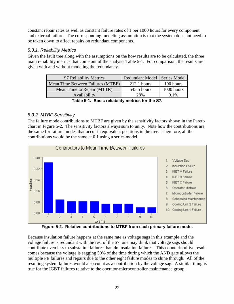
5.3.1. Reliability Metrics Given the fault tree along with the assumptions on the how results are to be calculated, the three main reliability metrics that come out of the analysis Table 5-1. For comparison, the results are given with and without modeling the redundancy.
S7 Reliability Metrics Redundant Model Series Model Mean Time Between Failures (MTBF) 212.1 hours 100 hours
Mean Time to Repair (MTTR) 545.5 hours 1000 hours Availability 28% 9.1%
Table 5-1. Basic reliability metrics for the S7.
5.3.2. MTBF Sensitivity The failure mode contributions to MTBF are given by the sensitivity factors shown in the Pareto chart in Figure 5-2. The sensitivity factors always sum to unity. Note how the contributions are the same for failure modes that occur in equivalent positions in the tree. Therefore, all the contributions would be the same at 0.1 using a series model.
Figure 5-2. Relative contributions to MTBF from each primary failure mode.
Because insulation failure happens at the same rate as voltage sags in this example and the voltage failure is redundant with the rest of the S7, one may think that voltage sags should contribute even less to substation failures than do insulation failures. This counterintuitive result comes because the voltage is sagging 50% of the time during which the AND gate allows the multiple PE failures and repairs due to the other eight failure modes to shine through. All of the resulting system failures would also count as a contribution by the voltage sag. A similar thing is true for the IGBT failures relative to the operator-microcontroller-maintenance group.
23
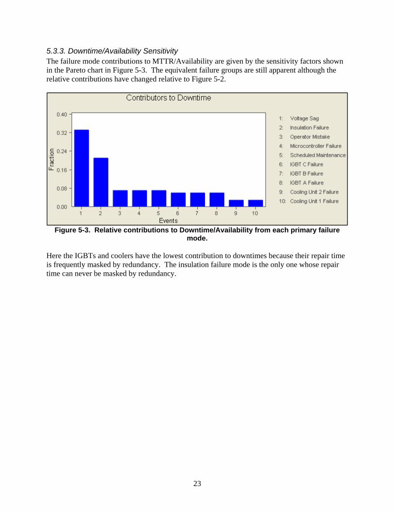
5.3.3. Downtime/Availability Sensitivity The failure mode contributions to MTTR/Availability are given by the sensitivity factors shown in the Pareto chart in Figure 5-3. The equivalent failure groups are still apparent although the relative contributions have changed relative to Figure 5-2.
Figure 5-3. Relative contributions to Downtime/Availability from each primary failure
mode. Here the IGBTs and coolers have the lowest contribution to downtimes because their repair time is frequently masked by redundancy. The insulation failure mode is the only one whose repair time can never be masked by redundancy.
24
6. OPTIMIZATION One of the most useful applications of reliability analysis is optimization. This example uses the previous example as the baseline from which to optimize.
6.1. Optimization in General As explained in Section 4.4, to set up an optimization problem, one has to define an objective function, list change options with their impacts, and define constraints. In general, the objective function will be a combination of several objectives. The options could involve discrete or continuous changes. The constraints could be hard or soft. In the latter case, they would be moved into the objective function. Once the problem has been set up, an optimization package is used to find good solutions. Objectives could be to: increase MTBFs or availability, or to reduce downtime, costs, size, or power dissipation. Options could be to: improve component reliability, insert new technology, redesign the system, or choose a mix of spare parts to keep on hand. Constraints could include: development budget, total component area/volume, total system weight, or implementation time. If the maximum budget to spend is a constraint, it obviously applies to whoever is choosing the options. But if minimizing cost is an objective, the optimum choice of options may depend on who bears that cost. In the case of PE systems, the manufacturer of the equipment may incur costs associated with design, redesign, fabrication, sales losses, or warranty claims. Electric utilities may incur the cost of parts, labor, loss of revenue, liability, fines, and increased regulation. Society may incur costs associated with loss of business, spoilage, safety, security, and public confidence. Optimization problems could be defined for any of these cases.
6.2. Application to the S7 This example was designed to convey the type of things optimization can do. Intuitively, we are trying how to allocate a fixed budget of reliability among the S7 components. Our objective is to increase the system MTBF. The options are to increase MTBFs of the individual components starting from 1,000 hours each (with downtimes fixed at 1,000 hours each). The specific “budget” constraint is a total component MTBF of 100,000 hours for the four component failure modes denoted by the colored leaves in Figure 5-1 (IGBT, cooler, microprocessor, and insulation). The external failure modes in the gray leaves are assumed to have fixed parameters. The objective function is called “fitness” since we are using a genetic algorithm (GA) to maximize it. The fitness function is some combination of total component MTBF and the resulting system MTBF. The GA is allowed to run for 29 generations as shown in the Figure 6-1.
25
Figure 6-1. Evolution of the fitness objective function over 29 generations.
Although the absolute scale doesn’t mean much, the small increase in fitness is enough to simultaneously maximize MTBF and satisfy the 100,000 hour total component lifetime constraint. The fitness appears to stop rising after 15 generations, but it doesn’t actually reach its maximum value until near the end of the simulation. The GA might still find an even better solution by running longer. As calculated in Section 5.3.1, MTBF starts at 212.1 hours with no hours yet spent on component upgrades. Figure 6-2 shows how the MTBF objective grows through the generations.
Figure 6-2. Maximizing the MTBF objective.
At the end of 29 generations, the system MTBF has reached a maximum of 709 hours. Even though most of the components have lifetimes over 10,000 hours, the maximum system MTBF is held down by the external failure modes in gray in Figure 5-1 which still have MTBFs of only 1000 hours.
Baseline Optimum
0.0951 0.104
Fitness
Baseline Optimum
212.1 709
MTBF
26
Figure 6-3 shows how the total component life is optimally spent across the four component types.
Figure 6-3. Satisfying the total component MTBF constraint.
The total component MTBF starts out at 4000 hours and quickly jumps up to near the objective of 100,000 hours. Only after 15 generations does it allocate all 100,000 hours. Note that the insulation failure mode gets the greatest lifetime boost to 34,000 hours since it leads directly into the system failure at the root of the tree. Conversely, the coolers and IGBTs are left with the lowest lifetimes because of their redundancy.
Improve Mean Life
Insulation 34,000.00
Microcontroller 32,000.00
Cooler 14,000.00
IGBT 20,000.00
Total Life 100,000.00
27
7. PROGNOSTICS AND HEALTH MANAGEMENT The cost of PE ownership can be unnecessarily high if maintenance or replacement is done too early or too late. Waiting until a system fails can be very expensive, so PE systems are usually replaced well before the end of their useful life to avoid the risk of unscheduled downtime. PHM seeks to reduce the cost by using sensors to detect anomalies, diagnose problems, predict a time to failure, and manage subsequent maintenance and operations in such a way to optimize overall system utility and cost. This section discusses certain PHM issues to then show how optimization analysis can also be used to identify potentially worthwhile PHM opportunities to pursue in the first place.
7.1. Failure Detection Strategies Possible failure detection strategies are (1) simple notification, (2) condition monitoring (CM), (3) prognostics, or (4) system failure. If there is no communication to central power operations, either through the SCADA system or periodic manned inspections, then there will be no notification of redundant failures or nascent failures before the system fails. Otherwise, if there is redundancy in the system, some simple notification method is probably possible. It may be the case that an incipient failure will inevitably lead, after some period of time, to a serious failure: one capable of contributing to a system failure. An example would be a slow leak in a fluid system. If the delay between an incipient failure and a serious failure is short relative to the mean time between incipient failures, the two types of failures could be rolled together and the MTBFs added together for analysis purposes. Alternatively, the delay could be used as a potential leverage point to make use of CM systems through which basic sensors and data signal processing flags for maintenance the less serious, incipient failure. In the case of CM, no estimate of the time until the serious failure is given. Clearly, a greater delay between the detection of an incipient failure and the subsequent serious failure is desirable. In cases where advanced indications of the serious failure are more subtle or predictions of time-to-failure are desired for health management (HM) purposes, sophisticated prognostics in the form of added sensors and real-time algorithms would be needed to make the failure prediction. These possibilities are given in Table 7-1.
Communication Redundancy Incipient Failure Detection Strategy
Y Y Y Simple Notification
Y Y N Simple Notification
Y N Y CM (no HM)
Y N N Prognostics (HM possible)
N Y Y System Failure
N Y N System Failure
N N Y System Failure
N N N System Failure Table 7-1. Failure detection strategy dependencies.
28
7.2. Maintenance Strategies Possible maintenance strategies are (1) unscheduled downtime, (2) scheduled downtime, (2) delayed scheduled downtime, and (4) repair while running. If there is no prior warning of failure, not even a recommended regular replacement schedule, the only option is running to failure and then performing repairs during unscheduled downtime. If there is no redundancy in the failed component but there is prior warning, scheduled downtime before system failure is a possibility. If there has been a failure in a redundant component (and therefore prior warning), but it is not possible to repair the system without taking it down, then the scheduled downtime will be merely delayed. In the case of constant failure rate, a factor of redundancy only increases the MTBF by a factor of less than 1 ln , and it increases the MTBF even less in cases where there is wear-out and the constant failure rate assumption does not apply. Since ln is such a slowly growing function, the redundancy doesn’t help much relative to cases where another method of prior warning is possible (viz., prognostics or CM of incipient failures). The best possible case is if there has been a failure in a redundant component (and therefore prior warning) and it is possible to repair the system without taking it down. These possibilities are given in Table 7-2.
Prior Warning Redundant Run & Repair Maintenance Strategy
Y Y Y Repair While Running
Y Y N Delayed Scheduled Downtime
Y N N/A Scheduled Downtime
N Y Y Unscheduled Downtime
N Y N Unscheduled Downtime
N N N/A Unscheduled Downtime Table 7-2. Maintenance strategy dependencies.
7.3. Health Management In cases where prior warning is possible (especially if there are reasonable time-to-failure predictions), the question of how to manage the health of the equipment is important. Once an incipient failure is detected, when should the necessary maintenance be conducted? Should the equipment be scheduled for repairs or taken off line immediately? The full cost of the serious failure, the cost of getting a repair crew out with the necessary parts, upcoming operational states, as well as the estimated time to failure would all need to be taken into account.
7.4. Risk-Based Cost Optimization With the preceding sections as an introduction, we turn to the use of optimization to identify potential PHM opportunities. The idea is to define an objective function that reflects both high consequences and little chance of detecting the failure early enough to do something about it. Optimal allocation of failure rate improvements on a fixed budget will then tell us which failure modes are potentially worthwhile PHM candidates. Those failure modes whose failure rates are reduced the most by the optimization would equivalently be places where PHM would profitably detect the failures early.
29
Define a risk-weighted cost for failure mode by multiplying the probability of not detecting it early enough by the cost of system failure. Then define the objective function as the average annual cost of those failures. This really only makes sense for a series system, so any redundant sub-trees would have to be replaced by an equivalent primary failure mode. The annual cost can be reduced by making components more reliable or by lowering the probability of non-detection. Note that the party that has the budget to make improvements does not have to be the same as the party that bears the cost. The optimization will try to reduce the failure rates of the most expensive modes. PHM could accomplish exactly the same thing by increasing the probability of detection of the corresponding incipient failures in time to do something about it. Although we do not know the probability of not detecting each failure mode in advance, one possible model for the probability of non-detection is
where is the time delay between an incipient failure and a major failure, and is the inspection time interval. This functional form reflects the fact that the probability of detection on each inspection is not independent of earlier inspections but is more likely to miss a problem the more it was missed earlier. Figure 7-1 shows the how the probability of non-detection drops as a function of increasing time delay between an incipient failure and the subsequent serious failure.
Figure 7-1. Probability of non-detection as a function of failure prediction lead time.
PHM has the effect of increasing the time delay ( ) with the effect of increasing the probability of detection, 1 . Having more frequent inspections (reducing ) would clearly have the same effect. Adding a canary device that would make it easier to detect an incipient failure during regular inspections would also help.
0
0.2
0.4
0.6
0.8
1
0.01 0.1 1 10 100 1000 10000 100000
Pro
bab
ility
Time Since Incipient Fault (hours)
Probability of Nondetection Given a 24-Hour Inspection Interval
30
8. RECOMMENDATIONS This section contains some brief recommendations to the PE and electric utility industries on ways to reduce costs and improve reliability of future PE systems as well as to reduce the cost of operations and maintenance. Specifically, the key to reliability improvement is to collect data, and as much as permissible, make it available to the community at large. Data is required to do basic reliability analysis through CM to advanced PHM, so any efforts in this direction will pay off. Manufacturers of PE equipment should:
1. Make provisions to record system data and make it available to the utility operator wherever practicable (e.g., through the SCADA system). Operating state, device cycle counts, external event statistics, component failures, temperatures, voltages, currents, etc. should be collected as functions of time. If information storage is an issue, histograms could be saved just a few times per day. Some of the histograms could even be two-dimensional to collect correlations; for example, they could record the frequency of combinations of temperature and current or the count of switching events as a function of operational state.
2. Maintain a reporting system for data back from utilities for continuous improvement. Incentives might include member database access and service discounts.
Electric utilities should:
1. Warehouse detailed maintenance data along with any data the manufactures provide. The maintenance data should include the sorts of fields described in Section 3.1.
2. Promote data collection understanding and buy-in for maintainers. In order to achieve the greatest possible accuracy and compliance, those maintaining the equipment need to understand what the data is being collected for and why it is important.
31
9. CONCLUSIONS This report has presented a general process for analyzing the reliability of any PE system. As we have seen, a number of assumptions and approximations have been made along the way. Even though the resulting models are not an exact representation of the equipment’s reliability characteristics, the reliability analysis process has many benefits. Continuing from the introduction (Section 1), the report has helped to illustrate that the process can also:
8. Encourage engineers to be explicit about reliability modeling assumptions and the data needed.
9. Reveal some unintuitive facts about the causes of unreliability, unavailability, and cost. 10. Show the relative importance of each type of failure mode. 11. Show how important external factors are relative to inherent reliability. 12. Help identify reliability problems at design time or after operations have begun. 13. Show where uncertainty in parameter estimates really matter to the final results. 14. Reveal areas where it might be profitable to pursue CM or prognostics.
Improvements in hardware and software technology are certainly essential to increase PE reliability. However, this report has shown that a systems view and judicious analysis can also help guide those improvements. Further development, dissemination, and adoption of analysis processes such as that presented here will further serve to enhance the reliability of PE and thereby help to enable the future electric grid.
32
10. REFERENCES 1. Office of Electricity Delivery and Energy Reliability, “Power Electronics Research and
Development Program Planning Document,” U.S, Department of Energy, Draft Document circa 2008 (http://www.ornl.gov/sci/electricdelivery/pdfs/PE_PP.pdf).
2. Sandia National Laboratories, Analyzing Field Data: User Manual for Pro-Opta Import Setup and Pro-Opta Data Analyzer. Sandia Corporation, Albuquerque, NM, April 2007.
3. Sandia National Laboratories, Design for Reliability: User Guide for Pro-Opta Fault Tree Interface, Pro-Opta Data Manager, and Pro-Opta Results Module. Sandia Corporation, Albuquerque, NM, April 2007.
4. Sandia National Laboratories, Optimization: User Manual for Pro-Opta Optimizer. Sandia Corporation, Albuquerque, NM, April 2007.
5. Campbell, James E., Longsine, Dennis E., and Atkins, Joel, “Algorithms for Treating Redundancy in Repairable and Non-Repairable Systems,” Sandia Report, SAND93-1822, October, 1993 (http://infoserve.sandia.gov/sand_doc/1993/931822.pdf).
33
DISTRIBUTION 1 MS1033 Stanley Atcitty 6336 10 MS1188 Mark A. Smith 6342 1 MS1188 Bruce M. Thompson 6342 1 MS 0899 Technical Library 9536 (electronic copy) 1 OE-10 Office of Electricity Delivery & Energy Reliability Attn: Gilbert Bindewald U.S. Department of Energy 1000 Independence Avenue, SW Washington, DC 20585