108
University of Toronto Power Management for VLSI Circuits Farid N. Najm University of Toronto [email protected]

University of Toronto
Power Management for VLSI Circuits
Farid N. Najm
University of Toronto

Outline
The Power Problem
Impact, issues, objectives, trends
Technology Trends and Projections
Historical trends (since 1960)
Future projections (up to 2020)
EDA for Power Management
Low-level power models
Power estimation and optimization
High-level power models
Bottom-up
Top-down
Conclusion
FMCAD-07 2Power Management for VLSI Circuits

FMCAD-07 Power Management for VLSI Circuits 3
The Power Problem
High frequency and chip density lead to high power
Today’s microprocessors consume 100-150 W
Future microprocessors may consume over 200 W
Power has an impact on:
System performance (battery life)
Chip performance (circuit speed)
Packaging and cooling (cost)
Signal integrity: Inductive kick (Ldi/dt), IR drop, noise, etc.
Physical reliability: Electromigration, hot-carriers, etc.
Power is a problem in both portable & fixed equipment

Impact on Performance
Power dissipation affects chip speed in two ways:
Power supply (voltage) variations (IR drop, Ldi/dt drop)
Temperature variations
Power supply reduction causes a circuit to slow down
A 5% reduction in Vdd may cause a 15% increase in gate delay
FMCAD-07 Power Management for VLSI Circuits 4
Id
Vdd
Idd+ -
Vdrop
Increased temperature has a
complex effect on speed
Traditionally: slow down
Today: gates speed-up, wires slow down
Overall result depends on the “mix”
Speed-up is not necessarily a good
thing, due to thermal runaway

FMCAD-07 Power Management for VLSI Circuits 5
Cooling/Packaging Cost
$$$
$$$
Energy
Tj Ta
avgthaj PRTT

FMCAD-07 Power Management for VLSI Circuits 6
Impact on Signal Integrity
Power supply current transients
cause:
Inductive kick due to Ldi/dt
IR drop due to line resistance
Leads to supply voltage glitches
and signal integrity problems:
Glitches get coupled to sensitive
analog or mixed signal nodes
Can cause dynamic circuits to loose
charge
Can cause latches to change state
Id
Vdd
Idd
+ -Ldi/dt

FMCAD-07 Power Management for VLSI Circuits 7
Impact on Chip Reliability
ICs are subject to a variety of
physical failure mechanisms:
Electromigration (EM)
Hot-carrier degradation (HC)
Other
Reliability is worse under:
High switching activity
High temperature
Result: chip MTF is reduced
under high power conditions
Voiding in metal1 due to electron wind from right-to-left through via.
Electromigration Damage

FMCAD-07 Power Management for VLSI Circuits 8
Power 101
p
n Cn
Cp
tot n pC C C
Q C Vlh n dd Q C Vhl p dd
lh hl lh hl tot ddQ Q Q C V
2
01 10 lh dd hl dd tot ddE E Q V Q V C V
212avg tot ddE C V (average energy per logic transition)
ddV
2
avg tot ddP C V f (average power at frequency: f )
Average power depends on:
switching frequency
supply voltage (squared)
transistor or gate count (C)

FMCAD-07 Power Management for VLSI Circuits 9
Bottom Line
Power has become a primary design concern
As part of a low-power design methodology, tools are
needed to accomplish several tasks:
Power Modeling and Characterization
Levels: MOSFET, gate, cell, macro, core, memory, IO
Objectives: static, average, RMS, peak power
Power Estimation (Analysis)
At all levels and for all objectives
Power Optimization (Synthesis)
At all levels and for all objectives
High-level tools are highly desirable

FMCAD-07 Power Management for VLSI Circuits 10
Power Depends on Workload
Power, much more so than delay, depends on what
stimulus is applied to the circuit, i.e., power is:
Pattern-dependent
Mode-dependent
Workload-dependent
Example: Running MS-Word on a laptop requires much
less power than running a 3D video game
For power estimation, reasonable accuracy is possible
only when the mode of operation is understood

FMCAD-07 Power Management for VLSI Circuits 11
Power Analysis Objectives
Different power objectives:
Transient power (waveform over time) v.s. average power
Use transient power for IR drop, power bus sizing, signal
integrity, physical reliability, etc.
Sometimes, only interested in peak power
May be interested only in highest current slope
Use average power for package selection, battery life, temperature
analysis, etc.
Static power v.s. dynamic power
It is possible to talk about the transient static power,
and the average static power
Static power is pattern-dependent (it’s not exactly DC)
P(t)
t

FMCAD-07 Power Management for VLSI Circuits 12
Dynamic Power
Dynamic power is consumed
when signals are
switching, and is due to:
Short-circuit current, also called
crowbar, or rush-through current
Current to charge internal nodes
Current required to charge output
and loading capacitance
Best understood as dynamicenergy per transition

FMCAD-07 Power Management for VLSI Circuits 13
Static Power
Static power consists of:
Off-current (leakage)
Sub-threshold current
Gate oxide leakage
pn-junction leakage
Standby current (sneak
paths, pull-ups, trickle
devices, sense-amplifiers)
0
2000
4000
6000
8000
10000
12000
14000
16000
1 3 5 7 9
11
13
15
17
19
Leakage Power (x 2.3 nW)
Nu
mb
er
of
Vecto
rs
In CMOS, leakage can be large:
1996: 100 MHz DSP core: 10%
1998: 600 MHz Alpha uP: 2W/72W
2002: 90nm FPGA: 10W
2006: 65nm 2-core Itanium: 40%
Future: 50% ?
Leakage, being exponential in
Vth, is the key reason why Vdd
will not scale any more!

Outline
The Power Problem
Impact, issues, objectives, trends
Technology Trends and Projections
Historical trends (since 1960)
Future projections (up to 2020)
EDA for Power Management
Low-level power models
Power estimation and optimization
High-level power models
Bottom-up
Top-down
Conclusion
FMCAD-07 14Power Management for VLSI Circuits

Moore’s Law
Empirical observation by Gordon Moore, 1965: “the number of transistors on a chip [for minimum component cost] doubles about every two years”
This exponential trend has fueled economic expansion on a global scale
Very few things in nature are “exponential”
Things cannot grow exponentially forever!
Source: http://www.intel.com/technology/mooreslaw/
FMCAD-07 15Power Management for VLSI Circuits

FMCAD-07 Power Management for VLSI Circuits 16
Microprocessor Performance
386486
Pentium(R)
Pentium Pro
(R)
Pentium(R)
IIMPC750
604+604
601, 603
21264S
2126421164A
21164
21064A
21066
10
100
1,000
10,000
19
87
19
89
19
91
19
93
19
95
19
97
19
99
20
01
20
03
20
05
Mh
z
1
10
100
Ga
te D
ela
ys
/ C
lock
Intel
IBM Power PC
DEC
Gate delays/clock
Processor freq
scales by 2X per
generation
Source: Intel

FMCAD-07 Power Management for VLSI Circuits 17
1998 DEC Alpha 21264
0
10
20
30
40
50
60
70
80
Po
we
r (W
)
0 100 200 300 400 500 600
Frequency (MHz)
Average Power Dissipation
0.35 , 2.2V
Rth=0.3 C/W
2W at DC, mostly leakage
Max 95W at 600MHz72 W, 33 A, at 600 MHz
15.2 Million Transistors, 3.14 cm2

FMCAD-07 Power Management for VLSI Circuits 18
1998 DEC Alpha 21264
Power Breakdown at 600 MHz
32%
18%15%
10%
10%
8%
5% 2%
Global Clock Network
Instruction Issue Units
Caches
Floating Execution Units
Integer Execution Units
Memory Management Unit
I/O
Miscellaneous Logic

FMCAD-07 Power Management for VLSI Circuits 19
Intel uPs, Maximum Power
0
10
20
30
40
50
1.5u 1u 0.8u 0.5u 0.35u 0.25u 0.18u
Process
Po
wer
(W
)
Pentium-II
Pentium Pro
Pentium
486386
Pentium/MMX
FMCAD-07 Power Management for VLSI Circuits 20
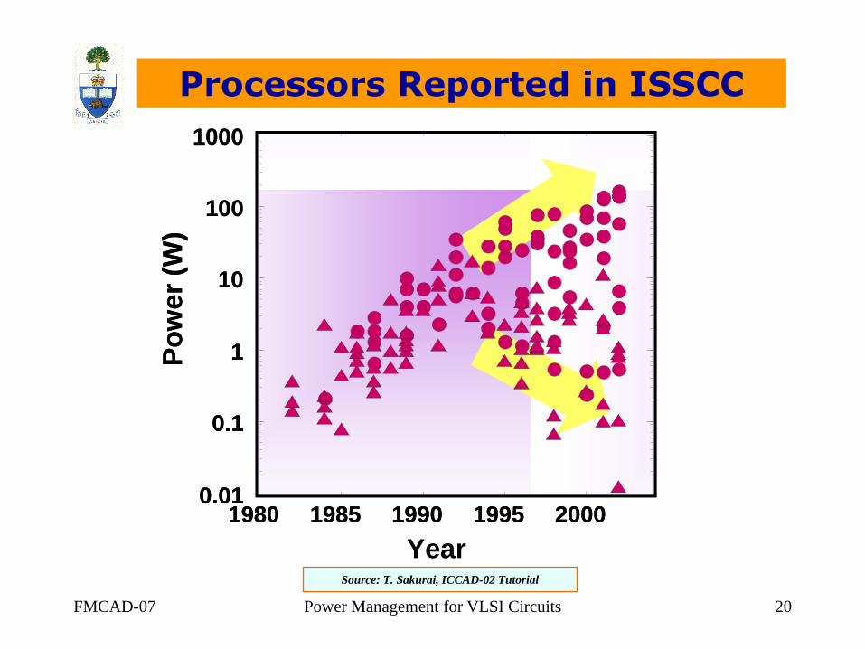
Processors Reported in ISSCC
Po
we
r (W
)
1980 1985 1990 1995 20000.01
0.1
1
10
100
1000
Year
Po
we
r (W
)
1980 1985 1990 1995 20000.01
0.1
1
10
100
1000
YearSource: T. Sakurai, ICCAD-02 Tutorial

FMCAD-07 Power Management for VLSI Circuits 21
Intel uPs, Power Density (1999)
1
10
100
1000
1.5u 1.0u 0.7u 0.5u 0.35u 0.25u 0.18u 0.13u 0.1u 0.07u
Process Generations
Watt
s/c
m2
Pentium III
Pentium II
Pentium Pro
Pentium
i486i386
Hot Plate
Nuclear Reactor
Rocket Nozzle
Pentium IV
(~1996)
(~2008)
(~2016)
Source: F. J. Pollack, “New microarchitecture challenges in the coming generations of CMOS process technologies,” 32nd Annual ACM/IEEE
International Symposium on Microarchitecture (Micro32), Haifa, Israel, p. 2, 1999. (Plenary Presentation)

FMCAD-07 Power Management for VLSI Circuits 22
Intel Leakage Trend (2000)
0
50
100
150
200
250
Technology
Po
wer
(Watt
s)
0%
20%
40%
60%
80%
100%
120%
Active Power
Leakage
Source (Intel paper): Kam, Rawat, Kirkpatrick, Roy, Spirakis, Sherwani andPeterson, “EDA challenges
facing future microprocessor design”, IEEE Transactions on Computer-Aided Design, Vol. 19, No. 12,
December 2000.

FMCAD-07 Power Management for VLSI Circuits 23
IBM Leakage Trend (2002)
Active-power
density
?
Subthreshold-power
density
0.01 0.1 1
Gate Length (um)
0.01
0.1
1
10
100
1000
0.001
0.0001
10-5
Pow
er
(W/c
m2)
E.J. Nowak. Maintaining the benefits of
CMOS scaling when scaling bogs down.
Volume 46, Numbers 2/3, Page 169
(2002)

FMCAD-07 Power Management for VLSI Circuits 24
Intel di/dt Trend (2000)
Pentium
Pro (R)Pentium
(R)
486386
1.E+00
1.E+01
1.E+02
1.E+03
1.E+04
1.E+05
1.E+06
1.E+07
1.E+08
di/
dt
in A
U
Source (Intel paper): Kam, Rawat, Kirkpatrick, Roy, Spirakis, Sherwani andPeterson, “EDA
challenges facing future microprocessor design”, IEEE Transactions on Computer-Aided Design, Vol.
19, No. 12, December 2000.

Outline
The Power Problem
Impact, issues, objectives, trends
Technology Trends and Projections
Historical trends (since 1960)
Future projections (up to 2020)
EDA for Power Management
Low-level power models
Power estimation and optimization
High-level power models
Bottom-up
Top-down
Conclusion
FMCAD-07 25Power Management for VLSI Circuits

Power Management for VLSI Circuits
Feature Size
Source: ITRS-05 & 06, http://public.itrs.net.
0
20
40
60
80
100
120
140
160
2000 2005 2010 2015 2020
Years
nan
o-m
ete
rs
DRAM 1/2 pitch MPU/ASIC M1 1/2 pitch
FMCAD-07 26

Power Management for VLSI Circuits
Functionality
Source: ITRS-05 & 06, http://public.itrs.net.
1
10
100
1000
10000
100000
2000 2005 2010 2015 2020 2025
Years
Mil
lio
n T
ran
sis
tors
/ch
ip
0.1
1
10
100
1000
DR
AM
Gig
a-b
its/c
hip
MPU cost-perf MPU perf ASIC DRAM
FMCAD-07 27

Power Management for VLSI Circuits
Speed
Source: ITRS-05 & 06, http://public.itrs.net.
1
10
100
2000 2005 2010 2015 2020 2025
Lo
cal C
lock F
req
uen
cy (
GH
z)
Years
FMCAD-07 28

FMCAD-07 Power Management for VLSI Circuits 29
Power Dissipation (ITRS-03)
Source: ITRS-03, http://public.itrs.net.
0
3
6
9
12
15
18
21
0
50
100
150
200
250
300
350
2000 2005 2010 2015 2020
Max
imum
Pow
er (M
obile
) (W
)
Max
imum
Pow
er (D
eskt
op) (
W)
Years
High-perf Cost-perf Mobile

Power Management for VLSI Circuits
Power Dissipation (ITRS-06)
Source: ITRS-06, http://public.itrs.net.
0
3
6
9
12
15
18
21
0
50
100
150
200
250
2000 2005 2010 2015 2020 2025
Ma
xim
um
Po
wer
(Mo
bile
) (W
)
Ma
xim
um
Po
wer
(De
sk
top
) (W
)
Years
High-perf Cost-perf Mobile
FMCAD-07 30

Power Management for VLSI Circuits
Supply Voltage
Source: ITRS-05 & 06, http://public.itrs.net.
0
0.2
0.4
0.6
0.8
1
1.2
1.4
2000 2005 2010 2015 2020 2025
Years
Su
pp
ly V
olt
ag
e (
V)
High-performance
Low power
FMCAD-07 31
FMCAD-07 Power Management for VLSI Circuits 32
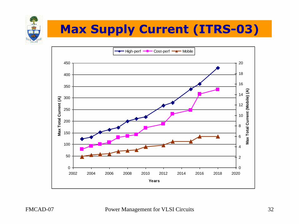
Max Supply Current (ITRS-03)
0
50
100
150
200
250
300
350
400
450
2002 2004 2006 2008 2010 2012 2014 2016 2018 2020
Years
Max T
ota
l C
urr
en
t (A
)
0
2
4
6
8
10
12
14
16
18
20
Max T
ota
l C
urr
en
t (M
ob
ile)
(A)
High-perf Cost-perf Mobile

Power Management for VLSI Circuits
Max Supply Current (ITRS-06)
0
2
4
6
8
10
12
14
16
18
20
0
50
100
150
200
250
300
350
2000 2005 2010 2015 2020 2025
Ma
x T
ota
l C
urr
en
t (M
ob
ile
) (A
)
Ma
x T
ota
l C
urr
en
t (A
)
Years
High-perf Cost-perf Mobile
FMCAD-07 33

Power Management for VLSI Circuits
Chip Pads
Source: ITRS-05 & 06, http://public.itrs.net.
0
1000
2000
3000
4000
5000
6000
7000
2000 2005 2010 2015 2020 2025
Years
Pad
Co
un
t
MPU Total MPU P/G (2/3) ASIC Total ASIC P/G (1/2)
FMCAD-07 34

Outline
The Power Problem
Impact, issues, objectives, trends
Technology Trends and Projections
Historical trends (since 1960)
Future projections (up to 2020)
EDA for Power Management
Low-level power models
Power estimation and optimization
High-level power models
Bottom-up
Top-down
Conclusion
FMCAD-07 35Power Management for VLSI Circuits

The Language of Power
Power modeling, estimation, and optimization methods
have been in development since the late 80s
A specialized terminology has developed
signal probability, static probability, transition
probability, entropy, state probability, conditional probability
switching activity, transition density, transition activity, toggle
rate, activity factor
spatial correlation, temporal correlation, spatio-temporal
correlation, pair-wise correlation, correlation factors
independence, conditional independence, lag-one model
bottom-up, top-down models, cycle-accurate
model, compaction
etc ...
FMCAD-07 Power Management for VLSI Circuits 36
Basics
In order to introduce basic power concepts, it is helpful
to consider the case of a single CMOS logic gate
The static power, Ps , for a given input vector, is the
constant power dissipated by the gate in steady state
when that vector is applied
Due to “off-current” (leakage)
The dynamic energy, Ed , for a given input (ordered)
pair of vectors is the energy dissipated in the gate due
to that vector transition.
Includes short-circuit, internal charging, and external charging
currents
Energy = QV = CV2 is measured in Joules, 1 J = 1 Watt-second
FMCAD-07 Power Management for VLSI Circuits 37

Avoid Double-Counting
During a transition, we must avoid mixing up the static
and dynamic components; here’s one way of doing this:
FMCAD-07 Power Management for VLSI Circuits 38
WPP
EE ssdtot
2
21
1sP2sP
)()( titv dddddE
W
)(tidd
)(tvdd

Power Vector Set
Power dissipation is well defined in connection with a
given input vector sequence, called a power vector set
Let Tpvs be the time duration of this vector set, then:
Transient power waveform is given by:
Average static power is given by:
Average dynamic power is given by:
FMCAD-07 Power Management for VLSI Circuits 39
)()( titv dddd
i
d
pvs
iET
)(1
pvsT
s
pvs
dttPT
0
)(1

Signal Statistics
Define: Indicator Function Ix(t) of a signal x(t) :
Ix(t) is 1 when x(t) is at logic high
Ix(t) is 0 when x(t) is at logic low
Ix(t) changes value instantaneously halfway through the
transition window duration W
Define: Signal Probability of a signal x(t) as the fraction
of time during which x(t) is high; formally:
The signal probability is a non-negative dimensionless
real number between 0 and 1.
FMCAD-07 Power Management for VLSI Circuits 40
pvsT
x
pvs
pvs dttIT
TxPxP0
)(1
),0;()(

Switching Activity
Define: Switching Activity of a signal x(t) as the average
number of logic transitions per unit time; formally:
where Nx(0, t) is the number of (complete) logic
transitions of the signal between 0 and t.
Other names for the switching activity:
switching rate, toggle rate, activity factor, transition
activity, and transition density
The switching activity is a non-negative real number
with units of transitions per second
FMCAD-07 Power Management for VLSI Circuits 41
pvs
pvsx
pvsT
TNTxRxR
),0(),0;()(

Outline
The Power Problem
Impact, issues, objectives, trends
Technology Trends and Projections
Historical trends (since 1960)
Future projections (up to 2020)
EDA for Power Management
Low-level power models
Power estimation and optimization
High-level power models
Bottom-up
Top-down
Conclusion
FMCAD-07 42Power Management for VLSI Circuits

Single Gate Power
Consider a gate with output node x, and let the static
power when x is low (high) be Ps0 (Ps1), then the
Average Static Power is:
Let Ed be the dynamic energy per transition, then the
Average Dynamic Power is:
FMCAD-07 Power Management for VLSI Circuits 43
)(1)(
))(1()(1
01
0 0
01,
xPPxPP
dttIPdttIPT
P
ss
T T
xsxs
pvs
savg
pvs pvs
)(),0(
, xRET
TNEP d
pvs
pvsxd
davg

Different Rise/Fall Energies
If the dynamic energy on a low to high transition is Ed,01
and is different from the dynamic energy on a high to
low transition Ed,10 , then:
If the initial state of the node is low, the expression for average
dynamic power becomes:
It is enough to talk about the average of Ed,01 and Ed,10 as the
average dynamic energy per transition, Ed
FMCAD-07 Power Management for VLSI Circuits 44
,01 ,10
,
,01 ,10
(0, ) 2 (0, ) 2
( )2
d x pvs d x pvs
avg d
pvs
d d
E N T E N TP
T
E ER x

Power and Capacitance
Let us ignore the internal power of a gate and focus on
the energy required to switch the output (drain and
interconnect) capacitance:
FMCAD-07 Power Management for VLSI Circuits 45
p
n Cn
Cp
pntot CCC
Q C Vlh n dd Q C Vhl p dd
lh hl lh hl tot ddQ Q Q C V
2
10,01, ddtotddhlddlhdd VCVQVQEE
)(2
21
, xRVCP ddtotdavg
ddV
212d tot ddE C V

Clocked Circuits
If the circuit is clocked, then it becomes convenient and
natural to normalize by the clock period
Let T be the clock period, and let Tpvs = NT, and let
t0=0, t1=T, t2=2T, …, tN=NT=Tpvs , then:
Thus, the signal probability is equal to the average fraction of a cycle in which the signal is high.
FMCAD-07 Power Management for VLSI Circuits 46
N
i
iipvs ttxPN
TxPxP1
1 ),;(1
),0;()(

Clocked Circuits
Switching activity is best normalized by the clock
frequency, leading to a revised definition :
Thus, the (normalized) switching activity is the average number of transitions per cycle, which is a dimensionless non-
negative real number
The two definitions are related by:
And the average dynamic power is now given by:
FMCAD-07 Power Management for VLSI Circuits 47
N
i
iix ttNN
xDxD1
1 ),(1
),0;()(
)()( xRTxD
, ( ) ( )avg d d dP E R x E D x f

The Zero-Delay Case
If all gates have zero-delay, then:
where Ix(i) is the indicator function evaluated at any time
during (but not at the start of) cycle i
So, the signal probability becomes: the average fraction of cycles in which the signal has a final value of logic high.
In this case, we also have:
where Pt(x) is the transition probability of x(t), defined as: the average fraction of clock cycles in which the final value of the signal is different from its initial value
FMCAD-07 Power Management for VLSI Circuits 48
N
i
xpvs iIN
TxPxP1
)(1
),0;()(
)()( xPxD t

Outline
The Power Problem
Impact, issues, objectives, trends
Technology Trends and Projections
Historical trends (since 1960)
Future projections (up to 2020)
EDA for Power Management
Low-level power models
Power estimation and optimization
High-level power models
Bottom-up
Top-down
Conclusion
FMCAD-07 49Power Management for VLSI Circuits

Power Estimation
At a low-level, power estimation requires computation
of the node switching activity R(x) or D(x)
A major difficulty is: pattern-dependence
The obvious solution approach is to use simulation:
Simulate a power-vector set to measure the toggle count
Combine with capacitance information to compute the power
Disadvantages: simulation is slow and expensive
Many attempts have been made to develop “static”
techniques to compute the power without simulation:
Analytical (probabilistic) methods
Monte Carlo (statistical) methods
FMCAD-07 Power Management for VLSI Circuits 50

Analytical Techniques
Propagate switching activity directly on the netlist
Key result: transition density propagation:
The partial derivative is the Boolean difference:
Probability computation is possible using a BDD
FMCAD-07 Power Management for VLSI Circuits 51
1
( ) ( )n
i
i i
yD y P D x
x
0 1( ) ( ) ( )
i ix xi
f x f x f xx
Logic Gate
or
Boolean Function
f(x)
x1
x2
xn
y

Analytical Techniques
A key assumption: inputs are uncorrelated
In practice, signals are often correlated, in complex ways
It is impractical to keep track of signal correlation
As a result, overall, these methods are inaccurate
Total large circuit accuracy within 10%
Local error can be much larger
Limited use:
Inside an optimization loop
Incremental analysis
FMCAD-07 Power Management for VLSI Circuits 52

Monte Carlo Techniques
Randomly select and simulate (only) short vector
sequences, from a large power-vector set
Use Monte Carlo theory to converge on the
mean, which is the average power
Although more accurate, these methods have not
displaced the simple simulation based approach
Dealing with unknown circuit state is a complication
The power vector set can itself be viewed as a collection of
“samples” and can be chosen small enough to simulate
The method of choice today remains simulation, and that remains unsatisfactory
FMCAD-07 Power Management for VLSI Circuits 53

Low-Power Synthesis
Incorporate power as an objective during synthesis
Practical experience shows that doing this during logic
synthesis is not very effective
This refers to standard logic synthesis, employing Boolean
optimizations followed by technology mapping
Once a circuit has been optimized for area, there is only 5-10%
further improvement to be had by further power optimization
It is generally agreed that optimizations at a higher level would have a higher impact
FMCAD-07 Power Management for VLSI Circuits 54

Design Techniques for Power
Despite nearly 20 years of research, there are no good truly EDA-driven solutions for power-aware design Power Estimation is still done by simulation
Low Power Logic Synthesis is ineffective
A number of “design techniques” have emerged: For dynamic power control:
Clock gating , dynamic frequency and/or voltage control, low-power libraries
Duplication and parallelism … multicore processor architectures
For leakage power control:
Multiple supply voltages and/or voltage islands, multiple Vth
transistors, sleep transistors and/or body bias control
While they benefit from EDA, the above techniques are not EDA-centric
FMCAD-07 55Power Management for VLSI Circuits

Duplication & Parallelism
Single core:
Reduce the supply voltage (slows down the circuit):
Run two identical copies in parallel at the lower (half)
frequency:
FMCAD-07 Power Management for VLSI Circuits 56
212avg tot dd avgP C V D f
2
12
2 2
ddavg tot avg
V fP C D
21 14 2avg tot dd avgP C V D f

Outline
The Power Problem
Impact, issues, objectives, trends
Technology Trends and Projections
Historical trends (since 1960)
Future projections (up to 2020)
EDA for Power Management
Low-level power models
Power estimation and optimization
High-level power models
Bottom-up
Top-down
Conclusion
FMCAD-07 57Power Management for VLSI Circuits

FMCAD-07 Power Management for VLSI Circuits 58
High-Level Power Models
Power estimation is required early in the design process
in order to:
Avoid costly redesign, in case the power is too high
Enable design exploration in a design-reuse environment
This requires power estimation at a high level of
abstraction
The key technology required is power models that can
be used at various levels of abstraction

FMCAD-07 Power Management for VLSI Circuits 59
Two Types of Power Models
Two types of models have been pursued:
Bottom-up (for hard macros)
Given complete low-level implementation, build a compact high
level model for power in terms of vector stimulus
Top-down (for soft macros)
Given a high-level functional description (and no low-level
implementation), along with a delay specification, a gate
library, and I/O switching activity, predict the required power
In practice, a high level design exploration environment
may need to mix both types of power models
Outline
The Power Problem
Impact, issues, objectives, trends
Technology Trends and Projections
Historical trends (since 1960)
Future projections (up to 2020)
EDA for Power Management
Low-level power models
Power estimation and optimization
High-level power models
Bottom-up
Top-down
Conclusion
FMCAD-07 60Power Management for VLSI Circuits

FMCAD-07 Power Management for VLSI Circuits 61
Bottom-Up Power Modeling
Logic block internal details are available
Generate a high level power macromodel :
Ward et al., Proc. IEEE, 1984
Powell and Chau, TCAS-91
Landman and Rabaey, TVLSI-95
Mehra and Rabaey, IWLPD-94
Mehta, Owens, and Irwin, DAC-96
Raghunathan, Dey, and Jha, ICCAD-96
Gupta and Najm, DAC-97
Qiu, Wu, Pedram, and Ding, ISLPED-97
etc. ...

FMCAD-07 Power Management for VLSI Circuits 62
Landman’s Method
Block power model is in terms of:
Block I/O statistics
Block structural attributes
Expert analysis is needed for a new type of function, in
order to determine:
The type of model required
The type of characterization needed

FMCAD-07 Power Management for VLSI Circuits 63
Example
For an SRAM with W words, & bit-width N :
The average capacitance switched per input bit, for a certain
transition ID, is modeled as:
The Ci coefficients are obtained by a process of
characterization and fitting
From this, the power is simply Pavg= CV2f
C C C W C N C WN0 1 2 3

FMCAD-07 Power Management for VLSI Circuits 64
Other Methods
Mehra’s method (with Rabaey):
Power model is Pavg= NaCaV2f, where:
Na is the average number of accesses to the resource, per cycle
Ca is the average capacitance switched per access
Even though Ca depends on input statistics, they compute it
up-front using UWN (Uniform White Noise)
System behavioral flowchart used to compute Na
Raghunathan’s method (with Dey and Jha):
Estimate activity and power in presence of glitching activity
They use both analytical and look-up tables
Power macromodel is built in terms of 9 or more variables

FMCAD-07 Power Management for VLSI Circuits 65
Our Approach
Power model : Pavg=DavgCtotV2f , where Davg is a
function of input statistics
What input statistics are sufficient to capture Davg over a
wide range of I/O data?
In terms of every input vector pair?
In terms of probability and activity at every input node?
Can we express Pavg in terms of aggregate input/output
statistics?

FMCAD-07 Power Management for VLSI Circuits 66
Aggregate Statistics
Use a fixed model template, on only 4 variables
Can be a LUT or equation-based using RLS
Model size is fixed, independent of circuit size
Variables are I/O switching activity statistics
Average input pin probability, Pin
Average input pin switching activity, Din
Average pair-wise input pin joint probability, SCin
Average output zero-delay pin switching activity, Dout
Characterization process is automatic, using simulation
No user intervention is required
Model evaluation is fast, based on the results of high-
level simulation

FMCAD-07 Power Management for VLSI Circuits 67
Spatial Correlation
Spatial correlation is defined as :
The 4-dimensional look-up table becomes :
Average error is 2-5%, worst case is -16% to +22%
{ 1}ij i jSC P x x
( , , , )avg in in in outP f P D SC D

FMCAD-07 Power Management for VLSI Circuits 68
Feasibility Region

FMCAD-07 Power Management for VLSI Circuits 69
Combinational Ckts - RLS

FMCAD-07 Power Management for VLSI Circuits 70
Sequential Circuits
State line statistics are implicit in the input vector
statistics, assuming correlation dies down over time

FMCAD-07 Power Management for VLSI Circuits 71
Cost of Characterization
Circuit #I #O #G Model Time #RLS
c499 41 32 202 C 16.31m 258
c880 60 26 383 Q 29.10m 162
c1355 41 32 546 C 22.2m 230
c1908 33 25 880 Q 36.14m 120
c432 36 7 160 Q 22.52m 163
c5315 178 123 2307 Q 3.74hrs 286
c2670 233 140 1193 C 2.24hrs 207
c3540 50 22 1669 Q 5.08hrs 228
c7552 207 108 3512 Q 19.75hrs 601
c6288 32 32 2406 C 9.23hrs 286

FMCAD-07 Power Management for VLSI Circuits 72
Cost of Characterization
Circuit #I #O #G #FF Model Time #RLS
s420 18 1 218 16 Q 56.96m 164
s641 35 24 379 19 Q 1.33hrs 179
s1196 14 14 529 18 Q 1.69hrs 2716
s510 19 7 211 6 Q 1.45hrs 147
s953 16 23 395 29 Q 5.5hrs 227
s298 3 6 119 14 Q 38.46m 288
s1238 14 14 508 18 Q 25.6m 456
s444 3 6 181 21 Q 22.2m 137
s820 18 19 289 5 Q 1.47hrs 141
s838 34 1 446 32 Q 2.86hrs 179
s5378 35 49 2779 179 Q 5.5hrs 89
s9234 36 39 5597 211 Q 14.64hrs 127

Outline
The Power Problem
Impact, issues, objectives, trends
Technology Trends and Projections
Historical trends (since 1960)
Future projections (up to 2020)
EDA for Power Management
Low-level power models
Power estimation and optimization
High-level power models
Bottom-up
Top-down
Conclusion
FMCAD-07 73Power Management for VLSI Circuits

FMCAD-07 Power Management for VLSI Circuits 74
Background
Estimation from a functional view is highly desirable
Early history: Two methods based on rough synthesis:
Muller-Glasser et al., ICCAD-91
Svensson et al., IWLPD-94
Function is synthesized as Boolean network, using
reference gates (eg. NAND2)
The gate count is multiplied by the average activity per
gate, estimated under UWN.
Subsequent work has explored other metrics, which
would not rely on rough synthesis

FMCAD-07 Power Management for VLSI Circuits 75
Estimation without Synthesis
Block internal details are not available
One approximation seems inevitable:
This approximation is very good in practice, leading to:
Both Davg and Ctot must be estimated from knowledge
of the input/output behavior only!
212avg tot dd avgP C V D f
1 1
( )N N
avg i i avg i avg tot
i i
P C D x D C D C

FMCAD-07 Power Management for VLSI Circuits 76
Our Approach
Power depends on the product of total capacitance and
average switching activity
Activity model:
Average internal activity in terms of average I/O activities
Several refinements
Capacitance model:
Computed as the product of:
Predicted average capacitance per gate
Predicted gate count
The resulting model is acceptable, but not final

FMCAD-07 Power Management for VLSI Circuits 77
Circuit Model
Assume the circuit is described in terms of:
Registers or flip-flops, and
Boolean equations for the combinational logic blocks
Combinational
Circuit
Registers
State lines
OutputsInputs
FMCAD-07 Power Management for VLSI Circuits 78
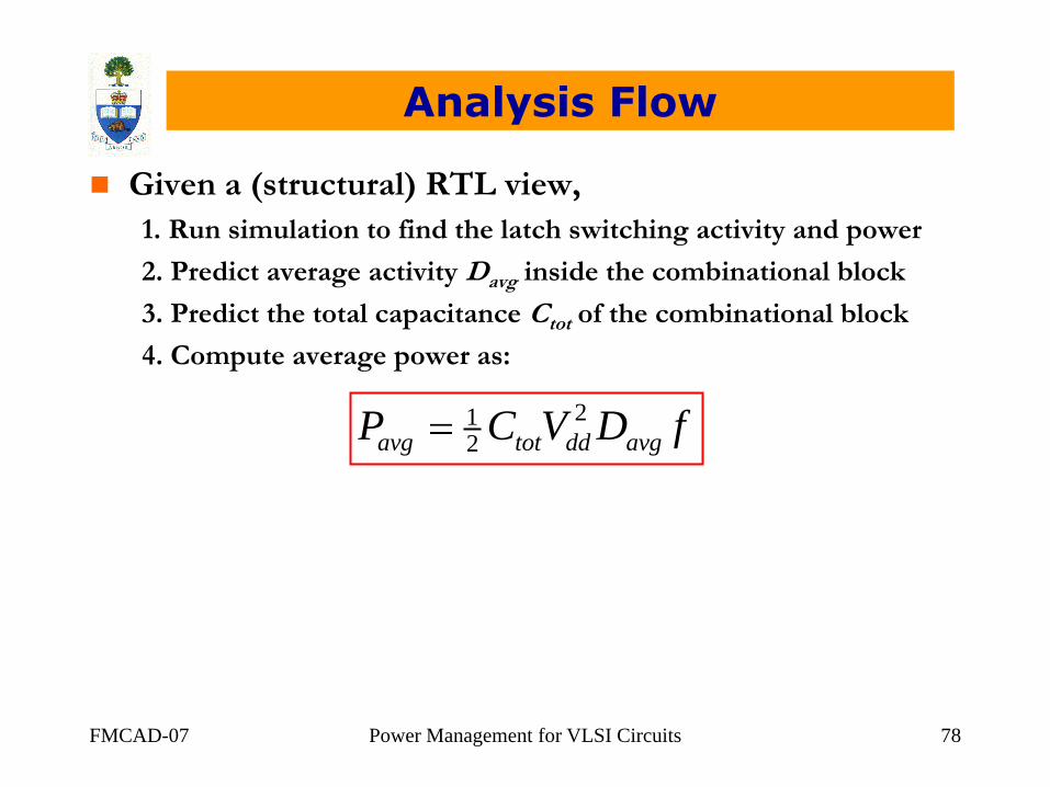
Analysis Flow
Given a (structural) RTL view,
1. Run simulation to find the latch switching activity and power
2. Predict average activity Davg inside the combinational block
3. Predict the total capacitance Ctot of the combinational block
4. Compute average power as:
212avg tot dd avgP C V D f

FMCAD-07 Power Management for VLSI Circuits 79
Average Activity Prediction
Study information transfer across the block:
Najm, ISLPD-95
Marculescu et al., ISLPD-95
Empirically, the scaled total switching activity per level
varies quadratically with circuit depth
This gives a model for the average switching activity
that depends only on I/O activity
This model gives zero-delay activity prediction only
We have also developed some refinements based on
pair-wise signal correlations

FMCAD-07 Power Management for VLSI Circuits 80
Average Activity Model
Assuming the quadratic behavior, this leads to:
where:
Di is the sum of the input switching activities
Do is the sum of the output switching activities
n is the number of input nodes
m is the number of output nodes
23 2avg i oD D D
m n

FMCAD-07 Power Management for VLSI Circuits 81
Zero-Delay Activity Results

FMCAD-07 Power Management for VLSI Circuits 82
Capacitance Prediction
Use Ctot = ACavg , where:
A is an estimate of the gate count of an “optimal” (in some
sense) implementation of the function
Cavg is the average gate + wire capacitance per gate
We have estimated A in two ways:
A theoretically appealing model that benefits from the structure
of the Boolean space of the function
A more practical empirical model based on Boolean networks
and tuning with a given synthesis flow
The practical model works better

FMCAD-07 Power Management for VLSI Circuits 83
Theoretical Approach
Area model:
Define complexity of a Boolean function
Consider Randomly Generated Boolean Functions (RGBF)
Characterize RGBFs synthesized in the target library for
dependence of area on function complexity
Typical logic functions exhibit similar dependence
For model evaluation, estimate complexity then use the RBGF
model to get the area
Limitations:
Not suitable for arithmetic blocks; good for control
Awkward concept of an output multiplexer and area recovery
Awkward handling of delay specification under synthesis
Model is expensive to evaluate

FMCAD-07 Power Management for VLSI Circuits 84
Area and Entropy
Early history: Entropy has been used to predicted area
of Randomly Generated Boolean Functions (RGBF)
For very small input count “n”, the average RGBF was
found to have area:
This model is empirical
As well, for very large “n”, it has been shown
theoretically that the area complexity is exponential
A Hn2

FMCAD-07 Power Management for VLSI Circuits 85
Previous Model is Unrealistic
When applied to moderate size functions that are
typical of VLSI, this model breaks down
Predicts an area of ~ 400 million gates, for a 32-input function
which can be built with 84 gates
The area function fitting was done for RGBFs with 25 inputs
Typical VLSI functions are very different from RGBFs -
they are not “average”

FMCAD-07 Power Management for VLSI Circuits 86
Our Model
In addition to entropy, we use the structure of the
Boolean ON-set/OFF-set of the function
Based on Average Cube Complexity C(f) :
Weighted average number of literals in a prime implicant
Obtained by random sampling and logic simulation
We have found that (approximately):
A HC f2 ( )

FMCAD-07 Power Management for VLSI Circuits 87
Limitations of Proposed Model
It is expensive to find the average cube complexity
This model breaks down for functions that contain
arrays of exclusive-or gates
This includes adders and multipliers
These circuits are perhaps best modeled via a bottom-up power
macromodel
This model is perhaps best suited for control-intensive
applications
The following results exclude XOR circuits

FMCAD-07 Power Management for VLSI Circuits 88
Area Prediction Technique
General procedure (for multi-output functions):
Transform to a single output function
Compute single-output function complexity
Compute single-output function area
Recover multi-output function area
f(n x m) mux(m x 1)

FMCAD-07 Power Management for VLSI Circuits 89
Single Output Area Model
0
100
200
300
400
500
600
2 3 4 5 6 7 8 9
Are
a (
ga
te c
ou
nt)
Complexity Metric
RGBF at H=0.68
VLSI at H=0.68

FMCAD-07 Power Management for VLSI Circuits 90
Area Recovery
A(f) = A( ) - Amux
lies between 0 and 1
The fraction, , depends on the average number of
control inputs in the prime implicants of
Based on this observation, an empirical model for
estimating was derived
f
f
f
f (n x m) mux (mx1)

FMCAD-07 Power Management for VLSI Circuits 91
Results
0
100
200
300
400
500
600
700
800
0 100 200 300 400 500 600 700
Pre
dic
ted
Are
a (g
ate
co
un
t)
Actual Area (gate count)

FMCAD-07 Power Management for VLSI Circuits 92
A More Practical Approach
Problem:
Previous method inaccurate and computationally expensive
Need fast and relatively accurate alternatives
Possible solution:
Use a Boolean Network (BN) representation of RTL
Pros: very easy to build and makes use of established graph
theoretical methods
Cons: not a canonical representation

FMCAD-07 Power Management for VLSI Circuits 93
Boolean Networks
Various measures can be defined to capture the
complexity of the BN
Node count, fan-in, fan-out, cut sets…
We need a complexity measure that
Is invariant for different BNs of the same Boolean function
Captures the gate count requirements of the actual circuit
Define area complexity measure as
where:
n : number of nodes in the BN
fin : average fan-in of the nodes in the graph
fout : average fan-out of the nodes in the graph
outin ffnBC )(

FMCAD-07 Power Management for VLSI Circuits 94
Complexity Measure
Can be written as
where:
fin : average fan-in of the BN
Rough measure of gate-count (silicon cost) of the node
Represents the amount of computation done in the nodes
Eout = n fout : total number of all outgoing edges
A measure of connectedness of the graph
Represents the overall communication in the graph
inout fEBC )(
FMCAD-07 Power Management for VLSI Circuits 95
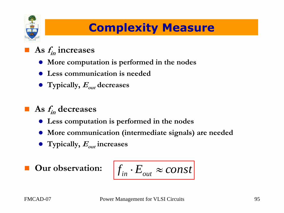
Complexity Measure
As fin increases
More computation is performed in the nodes
Less communication is needed
Typically, Eout decreases
As fin decreases
Less computation is performed in the nodes
More communication (intermediate signals) are needed
Typically, Eout increases
Our observation: constEf outin

FMCAD-07 Power Management for VLSI Circuits 96
Complexity Measure
0
500
1000
1500
2000
2500
C1355 C1908 C499 C880 alu2 apex6 example2 i5 my_adder ttt2
Co
mp
lexit
y M
easu
re
C(B) for different Boolean primitives
OR2
OR4
AND2
AND4
OR3/AND3

FMCAD-07 Power Management for VLSI Circuits 97
Complexity Measure
0
100
200
300
400
500
600
700
C1355 C1908 C499 C880 alu2 apex6 example2 i5 my_adder ttt2
No
de c
ou
nt
Node count for different Boolean primitives
OR2
OR3
OR4
OR5
OR6

FMCAD-07 Power Management for VLSI Circuits 98
Complexity Measure
0
500
1000
1500
2000
2500
3000
3500
4000
0 5000 10000 15000 20000 25000
Gate
Co
un
t
Complexity Measure - C(B)
Gate Count vs. C(B)

FMCAD-07 Power Management for VLSI Circuits 99
Gate Count Estimation Flow
Characterize the synthesis/mapping tool and the target
library (up-front one-time cost)
Choose a number of previously synthesized designs
Build the BNs corresponding to each
Compute the area complexity measure C(B)
Establish a model for the relationship between C(B) and the
gate-count (regression analysis, or look-up tables)
Gate count estimation
Build the BN for a new candidate design
Compute its area complexity measure
Using the above model, find the gate count

FMCAD-07 Power Management for VLSI Circuits 100
Results – Gate Count Estimation
0
200
400
600
800
1000
1200
1400
1600
1800
2000
0 200 400 600 800 1000 1200 1400 1600 1800 2000
Es
tim
ate
d G
ate
Co
un
t
Actual Gate Count
Using "Class" library

FMCAD-07 Power Management for VLSI Circuits 101
Results – Gate Count Estimation
0
200
400
600
800
1000
1200
1400
1600
0 200 400 600 800 1000 1200 1400 1600
Es
tim
ate
d G
ate
Co
un
t
Actual Gate Count
Using "Tc6a_core" library
FMCAD-07 Power Management for VLSI Circuits 102
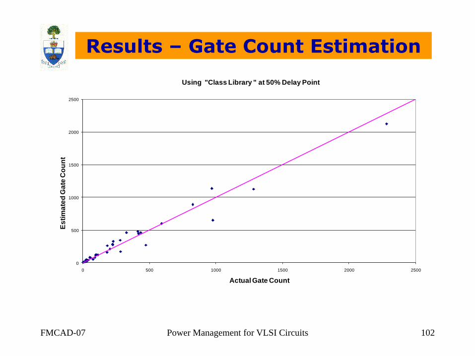
Results – Gate Count Estimation
0
500
1000
1500
2000
2500
0 500 1000 1500 2000 2500
Es
tim
ate
d G
ate
Co
un
t
Actual Gate Count
Using "Class Library " at 50% Delay Point

FMCAD-07 Power Management for VLSI Circuits 103
Capacitance Estimation Flow
Pre-computing Cavg (average capacitance per gate) for
the target library (characterization)
Obtain total capacitance for a number of synthesized designs in
the target library
Divide by gate count to obtain cavg for each circuit
Average these numbers to get Cavg for the library
Estimation of Ctot (total capacitance) for a given circuit
(estimation)
Estimate the gate count using the C(B) model
Obtain Ctot by multiplying the gate count by Cavg
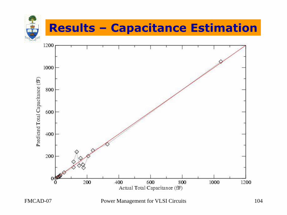
FMCAD-07 Power Management for VLSI Circuits 104
Results – Capacitance Estimation

FMCAD-07 Power Management for VLSI Circuits 105
Overall Power Estimation Flow
Read in:
The Boolean equations describing the design
The input statistics and delay constraints
Build a BN representation of the function
Estimate the gate count and the total capacitance
Run a zero-delay logic simulator to get the output
switching activity, Do, given the input activity, Di
Estimate the average (internal) switching activity
Estimate the power

FMCAD-07 Power Management for VLSI Circuits 106
Results (zero-delay power)

Outline
The Power Problem
Impact, issues, objectives, trends
Technology Trends and Projections
Historical trends (since 1960)
Future projections (up to 2020)
EDA for Power Management
Low-level power models
Power estimation and optimization
High-level power models
Bottom-up
Top-down
Conclusion
FMCAD-07 107Power Management for VLSI Circuits

Conclusion
Power is a primary concern for IC design
Dynamic power limits how fast we can clock an IC
Leakage power limits how much we can reduce the supply
Power is why the industry moved to CMOS 20 years ago
Power is why the industry is moving to multi-core processors
Several design techniques have been adopted to
mitigate the power problem
EDA contributions at the netlist/logic/RTL have had a
limited impact
It is felt that high-level early EDA intervention would
have a higher impact on the power of the final IC
FMCAD-07 Power Management for VLSI Circuits 108


