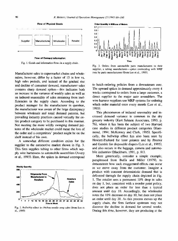
Creation and sale of goods often involves a num- ber of distinct firms operating in a serial time-line (Fig. 1). In a typical arrangement, suppliers provide raw materials to manufacturers, who provide finished goods to wholesalers, who combine many manufac- turers' products for sale to retailers, who then sell to the consumer of the product. In addition to the physical flow of goods downstream in the chain, there is an information flow that proceeds upstream. Only the retailer has direct contact with the ultimate consumer. The demand seen by wholesalers consists of orders from retailers, rather than consumers, and so on up the supply chain.
A number of firms in this environment have observed that distortions in demand information can occur as we proceed away from the consumer. For a number of reasons that will be discussed later, it has
been noticed that both the perceived demand season- ality and forecast error can increase as we proceed upstream in the supply chain. This distortion of demand in upstream activities is known variously as the "bul lwhip," "whip-saw," or "whip- lash" ef- fect (Lee et al., 1995). It is so called because a small variance or seasonality in actual consumer demand can "crack the whip" for upstream suppliers, caus- ing upstream suppliers to alternately produce at ca- pacity then experience downtime•
The bullwhip effect can have dramatic effects on companies that are removed from the end-user. Two specific examples are discussed here that relate to the experimental design later.
Fig. 2 depicts manufacturer's sales pattern and retailer's sales to the public of a major manufacturer of chicken noodle soup. Retail sales exhibit strong seasonality, with weekly sales differing by a factor of six between the high and low demand weeks•
90 R. Metters / Journal of Operations Management 15 (1997) 89-100
Flow of Physical Goods
Supplier Manufactur~ Wholesaler Retailer
Flow of Demand Information
Fig. 1. Goods and information flows in a supply chain.
Manufacturer sales to supermarket chains and whole- salers, however, differ by a factor of 15 in low vs. high sales periods, and instead of the gradual rise and decline of consumer demand, manufacturer sales contains sharp demand spikes--this indicates both an increase in the variance of weekly sales as well as an induced seasonality of sales stemming from inef- ficiencies in the supply chain. According to the product manager for the manufacturer in question, the manufacturer was aware of the large discrepancy between wholesale and retail demand patterns, but prevailing industry practices caused virtually the en- tire product category to be purchased in this manner. Not meeting the more wildly swinging demand pat- terns of the wholesale market could mean the loss of the order and a competitors' product might be on the shelf instead of his own.
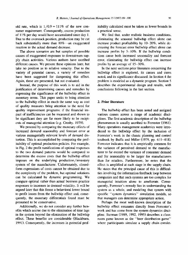
A somewhat different condition exists for the supplier to the automotive market shown in Fig. 3. This firm supplies tubing to other firms which sup- ply wire hamessess to automobile assemblers (Avery et al., 1993). Here, the spikes in demand correspond
Weekl Quantity 800
Shipments From /'~\ 600 Manufacturer to " ~ . . I \
Retailers " ~ 1 Retailers t Sales
400 :"':/ t / 200 ~
0 I ' ' ~ l ~ ' l , * l , , l , , I , , I , , l . t l ~ l . t . . l . l . , l * ~ l 4 7 10 13 16 19 22 28 28 31 34 37 40 43 46 41) 82
Time in Week
Fig. 2. Bullwhip effect in chicken noodle soup sales (from Lee et al., 1995).
Order Quantity In Millions of Meters 0.7
0.5
0.4
0.3
0.2
0.1
0
Time
Fig. 3. Orders from automobile parts manufacturers to their
supplier, a tubing manufacturer--spikes cooinciding with MRP runs by parts manufacturers (from Lee et al., 1995).
to batch-ordering policies from a downstream user. The upward spikes in demand approximately every 4 weeks correspond to orders from a large customer, a direct supplier to the major auto assemblers. The wire harness suppliers use MRP systems for ordering which order material once every month (Lee et al., 1995).
This phenomenon of induced seasonality and in- creased demand variance is common in the dry grocery industry (Kurt Salmon Associates, 1993, p. 76), where it has been the subject of two Harvard case studies in different product categories (Ham- mond, 1994; McKenney and Clark, 1995). Specifi- cally, the bullwhip effect has also been seen by Hewlett-Packard for laser printers and by Proctor and Gamble for disposable diapers (Lee et al., 1995), and also occurs in the luggage, camera and automo- bile industries (Blackburn, 1991, p. 81).
More generically, consider a simple example, paraphrased from Buffa and Miller (1979), to demonstrate how such exaggerated effects can occur as we move away from the customer. Imagine a product with constant deterministic demand that is delivered through the supply chain depicted in Fig. 1. The retailer sees a permanent 10% drop in sales on day 1, but, consistent with a reorder point policy, does not place an order for less than a typical amount until day 10. Accordingly, the wholesaler notes the 10% decrease on day 10, but does not place an order until day 20. As this process moves up the supply chain, the firm furthest upstream may not discover the decline in demand for several weeks. During this time, however, they are producing at the
R. Metters / Journal of Operations Management 15 (1997) 89-100 91
old rate, which is 1//0.9 = 111% of the new con- sumer requirement. Consequently, excess production of 11% per day would have accumulated since day 1. Due to the overstock position, production may be cut back substantially more than 10%--an exaggerated reaction to the actual demand decrease.
The above scenarios are but samples of possible causes of exaggerated responses to downstream sup- ply chain activities. Various authors have ascribed different causes. We present these opinions later, but take no position as to relative veracity. Due to the variety of potential causes, a variety of remedies have been suggested for dampening this effect. Again, these are presented, but not evaluated.
Instead, the purpose of this work is to aid in the justification of determining causes and remedies by expressing the significance of the bullwhip effect in monetary terms. This paper seeks to bring attention to the bullwhip effect in much the same way as cost of quality measures bring attention to the need for quality improvement programs: if the financial im- pact of inefficiencies can be measured and shown to be significant they are far more likely to be recipi- ents of managerial attention (e.g. Crosby, 1979).
We proceed by comparing the monetary effects of increased demand seasonality and forecast error at various managerially relevant levels of demand dis- tortion. This is accomplished by comparing the prof- itability of optimal production policies. For example, in Fig. 2 the profit ramifications of optimal responses to the two demand patterns would be compared to determine the excess costs that the bullwhip effect imposes on the underlying production/inventory system of the manufacturer. Unfortunately, closed- form expressions of costs cannot be obtained due to the complexity of the problem, but optimal solutions can be calculated by dynamic programming. We compare optimal rather than actual business practice responses to increases in demand volatility. It will be argued later that this forms a behavioral lower bound to profit losses from the bullwhip effect and, conse- quently, the monetary differentials found must be presumed to be conservative.
Additionally, we do not consider any further ben- efits which accrue due to the elimination of time lags in the system beyond the elimination of the bullwhip effect. These benefits are considerable (Blackburn, 1991). Consequently, the increases in potential prof-
itability calculated must be taken as lower bounds in a practical sense.
We find that, under realistic business conditions, eliminating the seasonal bullwhip effect alone can increase product profitability by 10-20%, while de- creasing the forecast error bullwhip effect alone can increase profits by 5-10%. If the bullwhip condi- tions cause both increased seasonality and forecast error, eliminating the bullwhip effect can increase profits by an average of 15-30%.
In the next sections prior literature concerning the bullwhip effect is explored, its causes and cures noted, and its significance discussed. In Section 4 the problem is modeled as a dynamic program. Section 5 describes the experimental design and results, with conclusions following in the last section.
2. Prior literature
The bullwhip effect has been noted and assigned various causes across a range of academic disci- plines. The first academic description of the bullwhip phenomenon is usually ascribed to Forrester (1961). Many operations management academics were intro- duced to the bullwhip effect by the inclusion of Forrester's work in the classic planning and control textbook by Buffa and Miller (1979, pp. 411-418). Forrester indicates that it is empirically common for the variance of perceived demand to the manufac- turer to far exceed the variance of consumer demand and for seasonality to be larger for manufacturers than for retailers. Furthermore, he notes that the effect is amplified at each stage in the supply chain. He states that the principal cause of this is difficul- ties involving the information feedback loop between companies and that such systems are too complex for managerial intuition alone to ameliorate. Conse- quently, Forrester's remedy lies in understanding the system as a whole, and modeling that system with specific "system dynamics" simulation models, so that managers can determine appropriate action.
Perhaps the most well-known description of the bullwhip effect emanates directly from Forrester's work and has come from the system dynamics disci- pline. Sterman (1989, 1992, 1995) describes a class- room game known as the "beer distribution game" where pariticipants simulate a supply chain consist-
92 R. Metters/ Journal of Operations Management 15 (1997) 89-100
ing of a beer retailer, wholesaler, distributor and brewery. As the game proceeds, a small change in a consumer demand invariably is translated into wild swings in both orders and inventory upstream. This game has been played many times over by students as well as executives in firms that are part of such supply chains and the result is still the same: exag- gerated responses occur upstream in the supply chain. These responses result in total system costs that are often five to 10 times the costs of optimal policies. Sterman (1989) and Diehl and Sterman (1989) char- acterize the reason for nonoptimal solutions in this game as poor decision making based on a lack of appreciation for the system as a whole. The poor decisions are deemed to come from difficulties in evaluating complex feedback loops in conjunction with time delays.
The beer game is well known and a useful teach- ing tool, but it may not be useful in obtaining accurate cost estimates of the bullwhip effect. Ster- man noted that one specific behavior participants exhibit is that they tend to order based on a per- ceived inventory position of on-hand inventory less backorders, rather than the correct view of inventory position being on-hand inventory plus on-order in- ventory less backorders. Although other factors are at work here as well, it is unlikely that this basic inventory position problem would occur in actual business practice with great regularity.
In a more expansive view of the same condition, Senge (1990) and Senge and Sterman (1992) use the beer distribution game as a prime example of empiri- cally observed managerial behavior and indicate that the bullwhip effect, in addition to many other man- agerial difficulties, is due to a lack of "system thinking" by management. Corrective action recom- mended by Senge and Sterman for this deficiency is a costly program of retraining managers.
Economists have also noted the bullwhip effect, but ascribe a different cause. Numerous studies of empirical data have all noted that the variance of production is greater than the variance of sales in a number of industries (Blinder, 1986; Blanchard, 1983; West, 1986; Krane and Braun, 1991). The reasons for this are variously described as the ratio- nal actions of profit optimizing managers responding to either demand shocks (Naish, 1994), stockout avoidance (Kahn, 1987), or production cost-smooth-
ing (Eichenbaum, 1989) to name only some of the potential reasons given.
Solutions to this problem are lacking in the above cited work as none of the authors seek to remedy the bullwhip effect, only to acknowledge the existence of the phenomenon and model the cause. We can, however, infer solutions by examining the causal agents. Largely, Naish (1994) and Kahn (1987) claim that ignorance of changes in end-user behavior cause the variance increases. Naish (1994) specifically ar- gues that if foreknowledge of demand changes are incorporated, the effect disappears. Consequently, it could be argued that investments in marketing and information systems that better appraise management of this behavior would alleviate the effect.
The bullwhip effect has not escaped the attention of researchers in operations management. Blackburn (1991, pp. 78-81) notes Forrester's prior work, but indicates that the overriding cause of the bullwhip effect--in addition to many other business problems - - i s the time delays between supply chain links. These time delays can be substantial, with average times quoted to be a year (Fisher and Raman, 1996, p. 87) to 66 weeks (Blackburn, 1991 p. 249) elapsing between supply orders and retail availability in the apparel industry and an average of 104 days in the dry grocery industry (Kurt Salmon Associates, 1993). Blackburn indicates that, among other results, fore- cast errors can be substantially reduced while sales are increased by compressing the time delays be- tween supply chain links.
Lee et al. (1994, 1995) have documented the effect in a number of specific businesses and have posited both causes and cures. In agreement with the economists, the bullwhip effect is purported to stem from rational, profit maximizing managers. Two spe- cific sources are claimed for the effect that are relevant for this research:
(1) Forward buying practices for seasonal items by downstream wholesalers and retailers amplifies the seasonality seen by the manufacturers. Fig. 2 is representative of such practices. As a general practice in the dry grocery industry, wholesale level buyers often induce larger seasonalities for manufacturers by purchasing overly large quanti- ties of product during the peak demand season for that product in an attempt to get reduced prices per unit.
R. Metters / Journal of Operations Management 15 (1997) 89-100 93
(2) Batching of orders by downstream participants. In Fig. 3, this is associated with MRP system ordering at month end, but it can also stem from the use of (s, S) systems. Demand may be rela- tively continuous by consumers, but due to order- ing costs or periodic ordering system runs it is batched early in the supply chain. This batching of orders induces demand variance up the supply chain that is not present at lower levels. A wide variety of corrective actions are recom-
mended, most of which involve the installation of information systems such as point of sale databases, EDI systems, etc.
3. Significance of the bullwhip effect
large (Blinder, 1986; Krane and Braun, 1991). All the econometric studies, however, are broad industry totals rather than finn or product specific results.
Lee et al. (1994, 1995) have specific product data that, although anecdotal, are more useful in deter- mining the scale of the effect and are used here in constructing the experimental design. In two specific corporate examples of increasing demand variance, the variance-to-mean ratios increased from 0.23 to 4.70 and 0.49 to 3.37 from consumer to manufac- turer demand. Although no simple metric exists for seasonality, some information may be obtained by comparing seasonal peaks. In two examples of in- duced seasonality (including the data in Fig. 2), manufacturer demand peaks were double and triple consumer sales peaks.
3.1. Empirical increases in demand distortion 3.2. Business profitability impacts
The purpose of this work is to demonstrate the significance of the bullwhip effect. The significance can be measured in two ways: the increase in param- eter values such as demand variance and seasonality, or the more consequential difference, the effects on overall business profitability. We first discuss the evidence concerning the magnitude of the increase in parameter values. Next, the central focus of this paper, estimating the decreased profitability due to the bullwhip effect, will be discussed.
In determining the magnitude of supply chain forecast error, Blackburn (1991, p. 250) indicates that forecast errors have, in practice, been cut in half by applying time-compression tactics, indicating the magnitude of potential decreases.
For a stronger statement concerning forecast er- ror, we first link the concepts of forecast error and empirically observed demand variance. For most probability distributions, given a series of random draws from a distribution, the best forecast of the next random draw would be the distribution mean. Empirically observed demand variance measures the deviation of actual demand from seasonally adjusted demand means and, consequently, provides a proxy for forecast error.
Such empirical observations have been obtained by the economists cited earlier. In industries that have a higher variance of production than sales variance, production variance is on average twice as
The distortions in perceived demand caused by the bullwhip may be intellectually interesting, but it is not clear that they are of practical interest. The monetary effect of such demand behavior as seen in Figs. 2 and 3 may or may not be significant. Given sufficient capacity, and technical conditions such as linear costs and deterministic demand spikes, such a demand pattern is no more costly than stationary demand. For example, consider two parallel situa- tions, one with known demand of 0 one week fol- lowed by demand of 1000 the next, compared to known demand of 500 both weeks. As long as capacity is greater than 1000 per week, and demand is deterministic, costs are identical in either case.
Even when demand is stochastic rather than deter- ministic, the overall increase in holding and shortage costs is closely approximated by a myopic policy (Lovejoy, 1990).
In business practice, however, two conditions pre- vail that cause the bullwhip effect to be of concern:
(1) manufacturers are typically capacitated; and (2) missing a customer deadline for a seasonal product often has ramifications in addition to the loss of revenue. Because of capacity considerations, meeting the
demand pattern in Fig. 3 requires carrying inventory in low demand weeks in anticipation of a demand spike. The demand pattern in Fig. 2 is more costly yet, as anticipatory inventory would have to be
94 R. Metters / Journal of Operations Management 15 (1997) 89-100
stockpiled long before the peak sales time to meet peak demand. As will be demonstrated later when discussing results, the combination of seasonality with capacitated systems cause the bullwhip effect to have significant cost effects.
Seasonal, capacitated systems are difficult to as- sess analytically. The cost functions of many unca- pacitated inventory scenarios can be expressed in a closed form equation. The optimal solution to the simpler uncapacitated, seasonal stochastic demand problem remains a complex algorithm (Zipkin, 1989). Capacity constrained stationary stochastic inventory systems also resist elegant solutions (Federgruen and Zipkin, 1986a,b), though some special cases have been solved (e.g. Ciarallo et al., 1994). Conse- quently, analytic cost comparisons must be made on a case by case basis from specifically calculated optimal policies, rather than by formula.
There are also difficulties in assessing such costs empirically. There are wide-ranging case study esti- mates that, for example, the grocery industry as a whole has $30 billion in excess inventory (Kurt Salmon Associates, 1993), the apparel industry has excess costs of $25 billion/year related to supply chain inefficiencies (Blackburn, 1991) or that Xerox was able to cut $1 billion in excess assets due to appropriate supply chain management (Lee et al., 1994). However, the relative contribution of the bullwhip effect vs. other factors is unclear.
4. Optimal policy calculation
Because of the difficulty of assessing such costs either empirically or by analytical closed-form ex- pressions, we address cost determination by a theo- retical comparison of optimal policies for example systems, where the optimal policies are determined by dynamic programming. We model the problem under consideration as a periodic, time-varying, stochastic demand dynamic program with capaci- tated production. We further assume that demand in excess of inventory incurs an additional penalty cost beyond lost revenue. This penalty cost is typically construed as lost sales. Lost sales is a more reason- able criterion than backordering in highly seasonal, capacitated businesses, where excess demand must be turned down since capacity is maximized in the
high demand season and customers no longer desire the goods once capacity is available. However, this cost can also be considered an additional cost for expediting, subcontracting, or other high marginal cost activities, combined with loss of customer good- will.
The purpose of problem modeling is to determine the cost of optimal production policies. Optimal policy costs are clearly lower bounds for the costs of heuristics used in business practice. We argue, how- ever, that the ratio of optimal policy costs in low variance, low seasonality environments vs. high vari- ance and seasonality environments is a behavioral lower bound for the cost ratios of business practice heuristics in low vs. high variance and seasonality environments. The limiting case of stochastic, time- varying demand is stationary demand with zero vari- ance. In this case, there is no reason for business practice production decisions to differ from optimal solutions. As variance and the time-varying proper- ties of demand increase, the situation becomes more complex managerially and business practice heuris- tics are likely to be in greater error. In the case of stochastic, seasonal demand it has been noted that businesses typically engage in far from optimal pro- duction plans (Bush and Cooper, 1988). Conse- quently, the ratio of high to low variance and season- ality optimal solutions should provide a conservative estimate of the actual costs of the bullwhip effect in practice.
Furthermore, efforts to reduce the bullwhip effect may include reducing the time delays between sup- ply chain links. This time compression itself causes less inventory to be held in transit. This corollary inventory reduction is in addition to the profitability model below.
The following notation is used to model a peri- odic, stochastic demand, capacitated production/in- ventory system. For time period t = 1,2 . . . . . the state and action variables, respectively, are:
i t inventory on hand at the beginning of the period Yt inventory on hand after production, but before
demand, where Yt >- it
We assume that demand, x t >_ 0, is stochastic and time dependent, independent between periods, and has a known probability distribution. We assume that the demand distribution parameters are time-varying.
R. Metters / Journal of Operations Management 15 (1997) 89-100 95
The general setting considers an unbounded planning horizon and discounted costs.
Define as follows:
&t(x) probability density function of demand in pe- riod t
~ t (x ) cumulative distribution function of demand in period t
t, revenue per unit h holding cost per unit per period 7r penalty cost per unit of unsatisfied demand in
addition to lost revenue c production cost per unit r units of scarce resource used to produce one
unit of product
R is the total units of scarce resource available in each period, and let c~ be the one period discount factor, 0 < ~ < 1. As is typical in such models, the costs of future decisions are discounted to avoid infinite costs in the general case of an infinite hori- zon.
The appropriate optimization can be characterized as a dynamic programming model (Zipkin, 1989; Federgruen and Zipkin, 1986a,b). For notational con- venience, we minimize costs rather than maximizing profit and treat revenue as a negative cost. Results, however, will be reported in terms of profit. Let jt(i t) denote the discounted expected cost that is incurred over an unbounded horizon when i t is the initial stock level and an optimal production rule is used. With time subscripts suppressed, we have
{ f0 y [ h ( y f ( i ) = m~n c ( y - i ) + -x ) -vx]4 , (x )
x d x + f f [ ~ r ( x - y) - vy] 4~( x)dx
So y, +a f(O)6(x)dx+ ( y - x ) 6 ( x )
X d x ] } s . t .y>_i ,y- i<R/r (1)
The function minimizes cost over Yt, the produce- up-to inventory position, subject to the conditions of non-negative production and production obeying ca- pacity constraints. Costs minimized are the sum of production, expected holding and excess demand
penalty costs and discounted future costs, less the effect of revenue. The form of the optimal solution to formulations similar to Eq. (1) has been shown to be that of a single critical produce-up-to number, Yt, that is the target point for the combination of produc- tion and entering inventory (Zipkin, 1989; Feder- gruen and Zipkin, 1986a,b).
5. Experimental design
We estimate the excess costs of the bullwhip effect by comparing the optimal solution costs of Eq. (1) under different parameter settings. We consider two distinct experimental designs corresponding to the analysis of Lee et al. (1994, 1995): (a) induced seasonality month by month on an annual basis caused by incorrect demand updating and forward contracts, depicted by Fig. 2; and (b) induced sea- sonality week by week on a monthly basis caused by order batching, depicted by Fig. 3. The former will be termed the "monthly analysis," the latter the "weekly analysis."
The monthly analysis assumes constant parameter values of r = l , h = l , a = 0 . 9 9 , c = 3 6 , v = 5 0 . This represents a product with a 40% profit margin over production costs, with a 33% annual holding cost and an annualized cost of capital of 13%, where each product unit requires one unit of capacity.
Varied quantities within both the monthly and weekly analysis include seasonality levels, demand variance, lost sales penalty costs, capacity levels and demand distributions.
The essential elements of the experimental design are the induced demand seasonality and demand variance caused by the bullwhip effect. Three de- mand seasonalities are used, with mean demand in each time period shown in Table 1. The values in Table 1 are chosen to correspond to actual business
Table 1 Monthly analysis: demand seasonality. Mean demand by time period
96 R. Metters / Journal of Operations Management 15 (1997) 89-100
practice. The ratio between the high and low demand points in the heaviest seasonality on Table 1 is 15:1, which corresponds to both the canned soup example in Fig. 2 and a similar example from a consumer product cited by Lee et al. (1995). The moderate seasonality level shown corresponds to the retail seasonality experienced in Fig. 2.
There is a constant variance-to-mean ratio in each time period. The variance-to-mean ratios are 0.5, 2 and 4. These variance-to-mean ratios correspond to two empirical examples cited by Lee et al. (1995) in the automotive and consumer goods industries.
Two demand distributions are used: uniform and a unimodal distribution 1. We vary penalty cost 7r = 0, 18, 36, so that the excess penalty for unsatisfied demand is only the loss of the profit margin, an additional 50% of production cost, or an additional 100% of production cost, respectively. Capacity is defined as a percentage of average cycle demand. Capacities of 125%, 150% and ~ are used. Since average demand per period is 12 for all seasonalities in Table 1, this corresponds to numerical values of capacity R = 15, 18 and ~. The number of experi- mental cells is 162 for the monthly analysis.
The weekly analysis has the constant parameter values r = 1, h = 1, ce = 0.9975, c = 156, v = 218. The parameter values differ from the monthly analy- sis because we now emulate weekly, rather than monthly decisions. The parameters are chosen to again represent a product with a 40% profit margin over production costs, with a 33% annual holding cost and an annualized cost of capital of 13%, where each product unit requires one unit of capacity.
We vary penalty cost 7r = 0, 78, 156, in accor- dance with the monthly analysis. Three demand sea- sonalities are used, with mean demand in each time period shown in Table 2. The heavy seasonality is chosen to represent the data on Fig. 3.
The variance-to-mean ratios, demand distributions and capacity levels used are identical to the monthly
Due to the mathematical requirements of unimodal distribu- tions, the negative binomial distribution is used for variance-to- mean ratios larger than 1 and the binomial distribution is used for variance-to-mean ratios less than 1. The uniform distribution is truncated where the mean and variance-to-mean ratio combination would cause negative demand.
Table 2 Weekly analysis: demand seasonality. Mean demand by time period
1 2 3 4
None 12 12 12 12 Moderate 8 8 24 8 Heavy 4 4 36 4
analysis, for a total of 162 additional experimental cells. The results of Eq. (1) are calculated for each experimental cell over 80 seasonal cycles. (Due to the discounting of future costs, beyond this point additional seasonal cycles cease to add meaningful costs.) Eq. (1) is coded in Turbo Pascal and the combined 324 experimental cells require 119 CPU hours on a Pentium 75 Mhz personal computer.
6. R e s u l t s
Standard statistical tools often used to evaluate results are not applicable here, as the costs are precise expected values found by dynamic program- ming, rather than statistical estimates.
We focus the reporting of results on the two factors that eliminating the bullwhip effect can en- hance: a decrease in demand seasonality or demand variance. Other experimental factors, such as capac- ity or the penalty cost for lost sales, are important firm or market characteristics, but are not altered by the bullwhip effect.
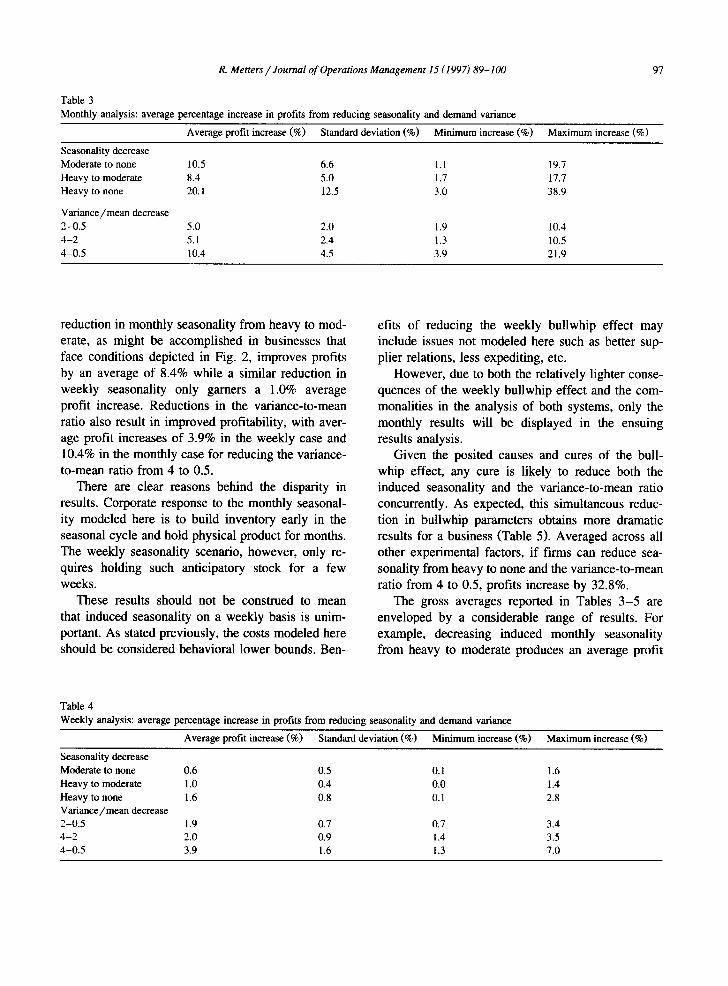
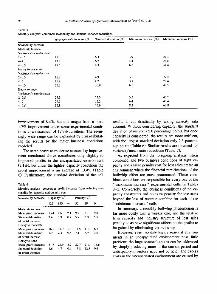
The percentage increase in optimal profits by reducing the bullwhip effect are summarized in Ta- bles 3 and 4. The results are averaged across all other experimental design parameters, so that each gross average in Tables 3 and 4 represents 108 experimental cells involving 54 matched pairs, and the minimum and maximum increases the largest and smallest number among those matched pairs. In gen- eral, reductions in the bullwhip effect can improve profits by large amounts, but the size of profit im- provement depends on both the cause of the bull- whip effect and associated business conditions.
The potential profit increases from dampening monthly seasonal changes far outweigh those that are associated with weekly seasonality. For example, a
R. Meners / Journal of Operations Management 15 (1997) 89-100
Table 3 Monthly analysis: average percentage increase in profits from reducing seasonality and demand variance
97
Average profit increase (%) Standard deviation (%) Minimum increase (%) Maximum increase (%)
Seasonality decrease Moderate to none 10.5 Heavy to moderate 8.4 Heavy to none 20.1
reduction in monthly seasonality from heavy to mod- erate, as might be accomplished in businesses that face conditions depicted in Fig. 2, improves profits by an average of 8.4% while a similar reduction in weekly seasonality only garners a 1.0% average profit increase. Reductions in the variance-to-mean ratio also result in improved profitability, with aver- age profit increases of 3.9% in the weekly case and 10.4% in the monthly case for reducing the variance- to-mean ratio from 4 to 0.5.
There are clear reasons behind the disparity in results. Corporate response to the monthly seasonal- ity modeled here is to build inventory early in the seasonal cycle and hold physical product for months. The weekly seasonality scenario, however, only re- quires holding such anticipatory stock for a few weeks.
These results should not be construed to mean that induced seasonality on a weekly basis is unim- portant. As stated previously, the costs modeled here should be considered behavioral lower bounds. Ben-
efits of reducing the weekly bullwhip effect may include issues not modeled here such as better sup- plier relations, less expediting, etc.
However, due to both the relatively lighter conse- quences of the weekly bullwhip effect and the com- monalities in the analysis of both systems, only the monthly results will be displayed in the ensuing results analysis.
Given the posited causes and cures of the bull- whip effect, any cure is likely to reduce both the induced seasonality and the variance-to-mean ratio concurrently. As expected, this simultaneous reduc- tion in bullwhip parameters obtains more dramatic results for a business (Table 5). Averaged across all other experimental factors, if firms can reduce sea- sonality from heavy to none and the variance-to-mean ratio from 4 to 0.5, profits increase by 32.8%.
The gross averages reported in Tables 3-5 are enveloped by a considerable range of results. For example, decreasing induced monthly seasonality from heavy to moderate produces an average profit
Table 4 Weekly analysis: average percentage increase in profits from reducing seasonality and demand variance
Average profit increase (%) Standard deviation (%) Minimum increase (%) Maximum increase (%)
Seasonality decrease Moderate to none 0.6 Heavy to moderate 1.0 Heavy to none 1.6 Variance/mean decrease 2-0.5 1.9 4 - 2 2.0 4-0.5 3.9
0.5 0.1 1.6 0.4 0.0 1.4 0.8 0.1 2.8
0.7 0.7 3.4 0.9 1.4 3.5 1.6 1.3 7.0
98 R. Metters / Journal of Operations Management 15 (1997) 89-100
Table 5 Monthly analysis: combined seasonality and demand variance reductions
Average profit increase (%) Standard deviation (%) Minimum increase (%) Maximum increase (%)
Seasonality decrease Moderate to none Variance/mean decrease 2-0.5 13.3 4-2 13.8 4-0.5 18.5 Heavy to moderate Variance/mean decrease 2-0.5 16.2 4-2 16.8 4-0.5 23.1 Heavy to none Variance/mean decrease 2-0.5 25.3 4-2 27.5 4-0.5 32.8
6.3 3.9 24.3 6.7 4.4 24.8 8.3 6.2 34.4
8.3 3.5 27.2 8.7 3.8 29.4 10.9 6.5 40.5
13.3 5.5 45.7 15.2 6.4 49.4 16.9 8.3 60.9
improvement of 8.4%, but this ranges from a mere 1.7% improvement under some experimental condi- tions to a maximum of 17.7% in others. The seem- ingly wide range can be explained by cross-tabulat- ing the results by the major business conditions
modeled. The same heavy to moderate seasonality improve-
ment mentioned above contributes only slightly to improved profits in the uncapacitated environment (2.1%), but under the tightest capacity conditions the profit improvement is an average of 13.4% (Table 6). Furthermore, the standard deviation of the cell
Table 6 Monthly analysis: percentage profit increases from reducing sea- sonality by capacity and penalty cost
Seasonality decrease Capacity (%) Penalty (%)
125 150 ~ 36 18 0
Moderate to none Mean profit increase 13.4 9.6 2.1 9.7 8.7 9.0 Standard deviation 2.4 1.9 0.2 5.7 5.0 5.5 of profit increase Heavy to moderate Mean profit increase 16.1 13.9 1.6 11.5 11.0 6.7 Standard deviation 1.9 2.3 0.5 7.1 6.9 3.6 of profit increase Heavy to none Mean profit increase 31.7 24.9 3.7 22.7 21.0 16.6 Standard deviation 4.6 4.7 0.6 13.8 12.8 9.6 of profit increase
results is cut drastically by taking capacity into account. Without considering capacity, the standard deviation of results is 5.0 percentage points, but once capacity is considered, the results are more uniform, with the largest standard deviation only 2.3 percent- age points (Table 6). Similar results are obtained for va r i ance /mean ratio reductions (Table 7).
As expected from the foregoing analysis, when combined, the two business conditions of tight ca- pacity and a large penalty cost for lost sales create an environment where the financial ramifications of the bullwhip effect are most pronounced. These com- bined conditions are responsible for every one of the " m a x i m u m increase" experimental cells in Tables 3 -5 . Conversely, the business conditions of no ca- pacity constraints and no extra penalty for lost sales beyond the loss of revenue combine for each of the " m i n i m u m increase" cells.
In summary, a monthly bullwhip phenomenon is far more costly than a weekly one, and the relative firm capacity and industry structure of lost sales penalty costs have significant effects on the profits to be gained by eliminating the bullwhip.
However, even monthly highly seasonal environ- ments in an uncapacitated environment pose little problem: the huge seasonal spikes can be addressed by simply producing more in the current period and anticipatory inventory need not be held. The excess costs in the uncapacitated environment are caused by
R. Metters / Journal of Operations Management 15 (1997) 89-100
Table 7 Monthly analysis: percentage profit increases from reducing the variance/mean ratio by capacity and penalty cost
99
Variance/mean decrease Capacity (%) Penalty (%)
125 150 ~ 36 18 0
Variance/mean of 2-0.5 Mean profit increase 6.1% 5.3% 3.9% 6.3% Standard deviation of profit increase 2.3 2.3 2.1 2.8 Variance/mean of 4-2 Mean profit increase 5.9 5.3 3.9 6.4 Standard deviation of profit increase 2.0 1.9 2.1 2.2 Variance/mean of 4-0.5 Mean profit increase 12.3 10.9 7.9 13.2 Standard deviation of profit increase 4.4 4.3 3.6 5.1
5.4% 3.6% 2.1 1.0
5.3 3.3 1.5 0.7
10.9 7.0 3.7 1.6
the reverse problem of anticipatory stock--if de- mand is less than expected, too much inventory may be available in the post-demand peak time periods. Furthermore, although the costs of such an uncapaci- tated environment are less in this analysis, adding capacity should not be viewed as a method for controlling the bullwhip effect. Clearly, adding ca- pacity includes substantial costs not modeled here. Additionally, this would not solve any root problems that may be causing more business problems than just the bullwhip effect.
7. Conclusions
The bullwhip effect is the amplification of both demand seasonality and variance as we proceed up- stream in a multiple finn supply chain. As a practical matter, the bullwhip effect is a well-documented problem that affects many businesses in serial supply chains across a variety of industries. Although it may seem an obvious inefficiency that is easy to correct, discovery of the bullwhip effect does not automati- cally lead to its solution: previous case studies IHammond, 1994; McKenney and Clark, 1995) demonstrate that, despite significant effort, the bull- whip effect can persist. Elimination of the bullwhip effect depends on altering well-established methods of doing business.
Although the precise causes of the bullwhip effect remain under debate, it is generally agreed that a lack of inter-company communication combined with
large time lags between receipt and transmittal of information are at the root of the problem. Conse- quently, solutions to the problem often involve in- creasing the abilities of companies to coordinate activity and cut lead times--which is typically ac- complished by both "sof t" means such as training, as well as by procurement of expensive MIS hard- ware such as point of sale and electronic data inter- change systems. The important point being that solu- tions to the bullwhip problem are expensive, and these expenses must be justified.
The purpose of this research is to assist in the justification of both practitioner and research interest in the bullwhip effect by determining the signifi- cance of the detrimental effect that the bullwhip effect can have on profitability. The approach taken here has been extremely cautious: we have delin- eated the benefits only of the amplified demand seasonality and variance that characterize the bull- whip effect. For example, a lead time reduction strategy that could eliminate the bullwhip effect would also generate significant savings in pipeline inventories and other costs, while generating addi- tional revenue through better attention to customer needs.
Despite this caution, results indicate that elimina- tion of the bullwhip effect can improve profitability in dramatic fashion. Utilizing managerially relevant parameter settings, eliminating demand distortions can improve profitability by several percentage points, making an investment in reducing demand distortions a highly profitable endeavor.
100 R. Metters / Journal of Operations Management 15 (1997) 89-100
Acknowledgements
The author wishes to acknowledge the guidance of J. Blackburn on this work.
References
C.N. Avery, M.A. Lariviere and J.M. Harrison, Raychem Corpo- ration, Thermofit Division (C): Demand Management, Case S-OIT-IC, Graduate School of Business, Stanford University, Stanford, CA, 1993.
J.D. Blackburn (ed.), The quick response movement in the apparel industry: a case study in time-compressing supply chains, in Time-Based Competition: The Next Battleground in American Manufacturing, Irwin, Homewood, IL, 1991, Chapter 11.
O.J. Blanchard, The production and inventory behavior of the American automobile industry, J. Polit. Econ., 91, 3 (1983) 365-400.
A.S. Blinder, Can the production smoothing model of inventory behavior be saved? Q. J. Econ., 101, 3, (1986) 431-454.
E.S. Buffa and J. Miller, Production-Inventory Systems: Planning and Control, Irwin, Boston, MA, 3rd edn, 1979.
C.M. Bush and W.D. Cooper, Inventory level decision support, Product. Inventory Manage. J., 29, 1 (1988) 16-20.
F.W. Ciarallo, R. Akella and T.E. Morton, A periodic review, production planning model with uncertain capacity and uncer- tain demand--optimality of extended myopic policies, Man- age. Sci., 40, 3 (1994) 320-332.
P.B. Crosby, Quality is Free, McGraw-Hill, New York, 1979. E. Diehl and J.D. Sterman, Effects of feedback complexity on
M.S. Eichenbanm, Some empirical evidence on the production level and production cost smoothing models of inventory investment, Am. Econ. Rev., 79, 4 (1989) 853-864.
A. Federgruen and P.H. Zipkin, An inventory model with limited production capacity and uncertain demands. I. The average-cost criterion, Math. Ops Res., 11, 2 (1986a) 193-207.
A. Federgruen and P.H. Zipkin, An inventory model with limited production capacity and uncertain demands. II. The dis- counted-cost criterion, Math. Ops Res., 11, 2 (1986b) 208- 216.
M.L. Fisher and A. Raman, Reducing the cost of demand uncer- tainty through accurate response to early sales, Ops Res., 44, 1 (1996) 87-99.
J.W. Forrester, Industrial Dynamics, MIT Press, Cambridge, MA, 1961.
J.H. Hammond, Barilla SpA (A), Case N9-694-046, Harvard Business School Publishing, Boston, MA, 1994.
J.A. Kahn, Inventories and the volatility of production, Am. Econ. Rev., 77, 4 (1987) 667-679.
S.D. Krane and S.N. Braun, Production smoothing evidence from physical product data, J. Polit. Econ., 99, 3 (1991) 558-581.
Kurt Salmon Associates, Efficient Consumer Response: Enhanc- ing Consumer Value in the Grocery Industry, Kurt Salmon Associates, Atlanta, GA, 1993.
H.L. Lee, P. Padmanabhan and S. Whang, Information distortion in a supply chain: the bullwhip effect, Working paper, Stan- ford University, Stanford, CA, 1994.
H.L. Lee, P. Padmanabhan and S. Whang, The paralyzing curse of the bullwhip effect in a supply chain, Working paper, Stanford University, Stanford, CA, 1994.
W.S. Lovejoy, Myopic policies for some inventory models with uncertain demand distributions, Manage. Sci., 36, 6 (1990) 724-738.
J.L. McKenney and T.H. Clark, Campbell Soup Co.: a leader in continuous replenishment innovations, Case 9-195-124, Har- vard Business School Publishing, Boston, MA, 1995.
H.F. Naish, Production smoothing in the linear quadratic inven- tory model, Q. J. Econ., 104, 425 (1994) 864-875.
P.M. Senge, The Fifth Discipline, Doubleday, New York, 1990. P.M. Senge and J.D. Sterman, Systems thinking and organiza-
tional learning: acting locally and thinking globally in the organization of the future, Eur. J. Opl Res., 59, 3 (1992) 137-145.
J.D. Sterman, Modeling managerial behavior: misperceptions of feedback in a dynamic decision making experiment, Manage. Sci., 35, 3 (1989) 321-339.
J.D. Sterman, Teaching takes off, flight simulators for manage- ment education, OR~MS Today, 19, 5 (1992) 40-44.
J.D. Sterman, The beer distribution game, in J. Heineke and L. Meile (eds), Games and Exercises for Operations Manage- ment, Prentice Hall, Englewood Cliffs, NJ, 1995, pp. 101-112.
K.D. West, A variance bounds test of the linear quadratic inven- tory model, J. Polit. Econ., 94, 4 (1986) 374-401.
P.H. Zipkin, Critical number policies for inventory models with periodic data, Manage. Sci., 35, 1 (1989) 71-80.