Journal of Business Studies Quarterly

2012, Vol. 3, No. 4, pp. 24-42 ISSN 2152-1034

REAL EXCHANGE RATE EQUILIBRIUM AND

MISALIGNMENT IN KENYA

Danson Musyoki

Ganesh P. Pokhariyal

Moses Pundo

University of Nairobi, Kenya

Abstract

This paper examines Real Exchange Rates (RER) misalignment in Kenya by using Johansen

Cointegration and error correction technique based on single equation and Vector

Autoregressive (VAR) specification. It was found that actual RER was more often above its

equilibrium value for the study period of June 1993 – December 2009 and the country’s

international competitiveness deteriorated over the study period.

Keywords: Real Exchange Rate, Misalignment, Equilibrium.

1.0 Introduction

Misalignment of the RER, whereby the actual RER deviates from equilibrium value, has

important implications on a country’s economic growth. RER overvaluation, for instance, would

be damaging to a country’s economic growth, as it would particularly hamper growth in all

sectors (Edwards, 1989, Gylfason, 2002). Such misalignment is widely believed to influence

economic behaviour. In particular, overvaluation is expected to hinder economic growth, while

undervaluation is sometimes thought to provide an environment conducive to growth.

An exchange rate is defined as a price at which one currency may be converted into

another. Exchange rate is referred to as the nominal exchange rate (NER) when inflation effects

are embodied in the rate, and as the real exchange rate (RER) when inflation influences have not

been factored in the rate (Copeland, 1989:4, Lothian, and Taylor, 1997).

During the era of the fixed exchange rate regime, that covered the period of 1966-92,

Kenya, like many developing countries, had to frequently devalue its currency in an attempt to

reduce the negative effects that RER misalignment had on its economy. The adoption of a

floating exchange rate system in 1993 marked the climax of efforts to make the RER more

aligned to the market determined equilibrium RER, and thus eliminate RER misalignment. There

is, however, no available evidence that success has since been achieved in realizing the objective

for which the foreign exchange market was liberalized.

In spite of the abundant literature on the effects of exchange rate volatility on

macroeconomic variables such as economic growth, studies that specifically focus on Kenyan

economy are scanty. Were et. al., (2001), analyzed factors that have influenced the exchange rate

Journal of Business Studies Quarterly

2012, Vol. 3, No. 4, pp. 24-42

©JBSQ 2012 25

movements since the foreign exchange market was liberalized in 1993. A related study by

Ndung'u (1999) assessed whether the exchange rates in Kenya were affected by monetary policy,

and whether these effects were permanent or transitory. The study by Kiptoo (2007) focused on

the real exchange rate, misalignment, and its impact on the Kenya’s international trade, and

investment. Sifunjo (2011) investigated chaos and nonlinear dynamical approaches to predicting

exchange rates in Kenya.

Few studies in Kenya too have attempted to estimate the RER equilibrium path, and use it

to provide any evidence on the nature and extent of exchange rate misalignment, and the

implications of such misalignment on Kenya’s economic growth. This study examines and

provide a deep understanding of equilibrium RER by not only investigating factors that

determine RER behaviour, but also measuring RER deviations from the equilibrium path.

Real Exchange Rate Misalignment

RER misalignment, refer to measures of deviations of actual RER from its long run or

equilibrium level. Therefore, the equilibrium RER is the RER that would be prevailing when an

economy is operating at full employment and maximum output, and its balance of payment

position is at sustainable level. Thus, misalignment in the RER is the difference between the

actual RER, and the equilibrium RER.

An exchange rate is labeled undervalued when it is more depreciated than the equilibrium

RER, and overvalued when it is more appreciated than the equilibrium RER (Edwards, 1989).

Determining the equilibrium RER is pivotal in computing the degree of misalignment. Policy

makers and many researchers are interested in predicting, and monitoring misalignment in the

foreign exchange market, because, in many cases, it is closely related to possible current account

problems or impending currency crises.

1.2 Exchange Rate Determination

There are at least five competing theories of the exchange rate concept, which may either

be classified as traditional or modern. These theories are: the elasticity approach to exchange rate

determination, the monetary approach to exchange rate determination, the portfolio balance

approach to exchange rate determination, and the purchasing power theory of exchange rate

determination. The modern theory explain the short run volatility of the exchange rate and their

ability to shoot in the long run.

1.3 Overview of Kenya’s Exchange Rate Policy and its economic impact

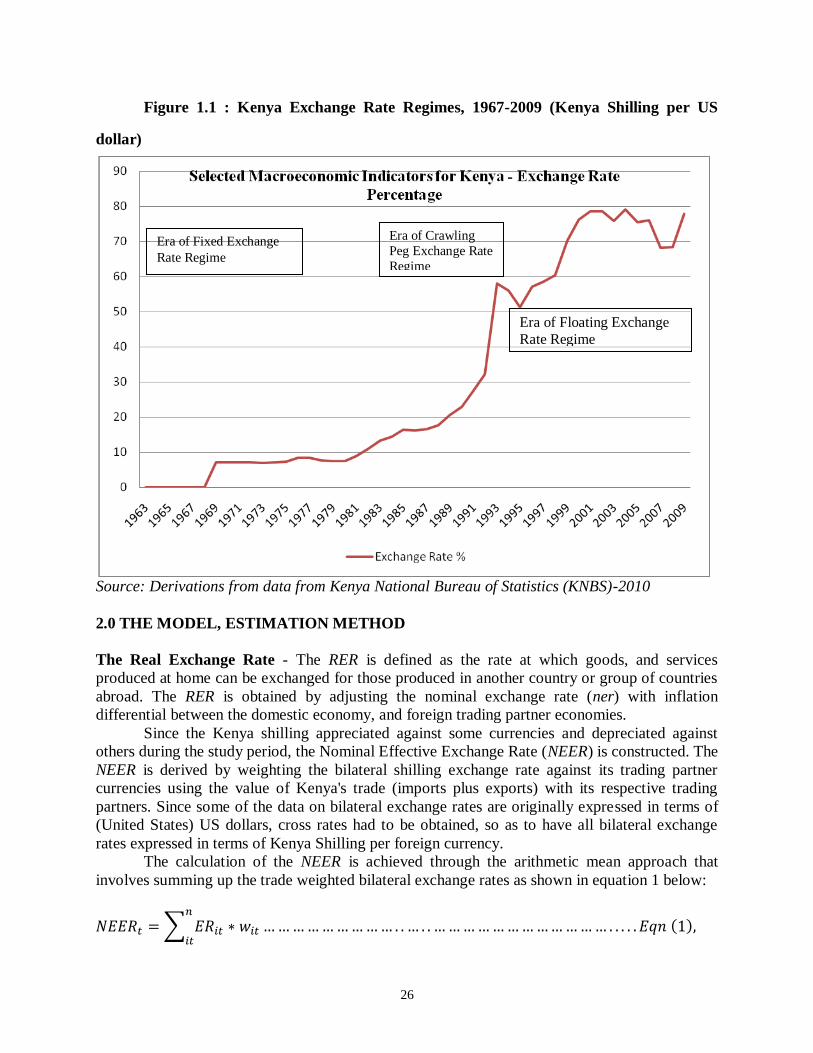
The exchange rate of Kenya shilling to the US Dollar from 1967 to 2009 has been

described by the fixed exchange rate error, the crawling peg error and the floating error.

26

Figure 1.1 : Kenya Exchange Rate Regimes, 1967-2009 (Kenya Shilling per US

dollar)

Source: Derivations from data from Kenya National Bureau of Statistics (KNBS)-2010

2.0 THE MODEL, ESTIMATION METHOD

The Real Exchange Rate - The RER is defined as the rate at which goods, and services

produced at home can be exchanged for those produced in another country or group of countries

abroad. The RER is obtained by adjusting the nominal exchange rate (ner) with inflation

differential between the domestic economy, and foreign trading partner economies.

Since the Kenya shilling appreciated against some currencies and depreciated against

others during the study period, the Nominal Effective Exchange Rate (NEER) is constructed. The

NEER is derived by weighting the bilateral shilling exchange rate against its trading partner

currencies using the value of Kenya's trade (imports plus exports) with its respective trading

partners. Since some of the data on bilateral exchange rates are originally expressed in terms of

(United States) US dollars, cross rates had to be obtained, so as to have all bilateral exchange

rates expressed in terms of Kenya Shilling per foreign currency.

The calculation of the NEER is achieved through the arithmetic mean approach that

involves summing up the trade weighted bilateral exchange rates as shown in equation 1 below:

Era of Fixed Exchange

Rate Regime

Era of Crawling

Peg Exchange Rate

Regime

Era of Floating Exchange

Rate Regime

Journal of Business Studies Quarterly

2012, Vol. 3, No. 4, pp. 24-42

©JBSQ 2012 27

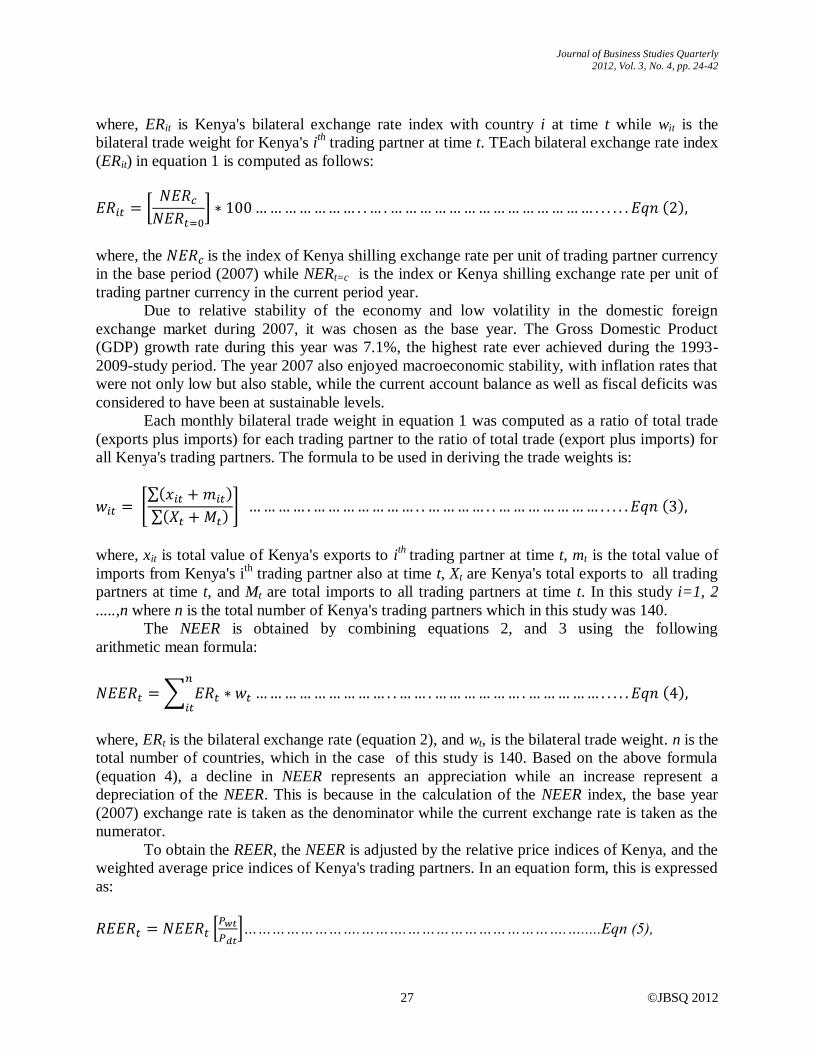
where, ERit is Kenya's bilateral exchange rate index with country i at time t while wit is the

bilateral trade weight for Kenya's ith

trading partner at time t. TEach bilateral exchange rate index

(ERit) in equation 1 is computed as follows:

where, the is the index of Kenya shilling exchange rate per unit of trading partner currency

in the base period (2007) while NERt=c is the index or Kenya shilling exchange rate per unit of

trading partner currency in the current period year.

Due to relative stability of the economy and low volatility in the domestic foreign

exchange market during 2007, it was chosen as the base year. The Gross Domestic Product

(GDP) growth rate during this year was 7.1%, the highest rate ever achieved during the 1993-

2009-study period. The year 2007 also enjoyed macroeconomic stability, with inflation rates that

were not only low but also stable, while the current account balance as well as fiscal deficits was

considered to have been at sustainable levels.

Each monthly bilateral trade weight in equation 1 was computed as a ratio of total trade

(exports plus imports) for each trading partner to the ratio of total trade (export plus imports) for

all Kenya's trading partners. The formula to be used in deriving the trade weights is:

where, xit is total value of Kenya's exports to ith

trading partner at time t, mt is the total value of

imports from Kenya's ith

trading partner also at time t, Xt are Kenya's total exports to all trading

partners at time t, and Mt are total imports to all trading partners at time t. In this study i=1, 2

.....,n where n is the total number of Kenya's trading partners which in this study was 140.

The NEER is obtained by combining equations 2, and 3 using the following

arithmetic mean formula:

where, ERt is the bilateral exchange rate (equation 2), and wt, is the bilateral trade weight. n is the

total number of countries, which in the case of this study is 140. Based on the above formula

(equation 4), a decline in NEER represents an appreciation while an increase represent a

depreciation of the NEER. This is because in the calculation of the NEER index, the base year

(2007) exchange rate is taken as the denominator while the current exchange rate is taken as the

numerator.

To obtain the REER, the NEER is adjusted by the relative price indices of Kenya, and the

weighted average price indices of Kenya's trading partners. In an equation form, this is expressed

as:

…………………….……….…………………………….….....Eqn (5),

28

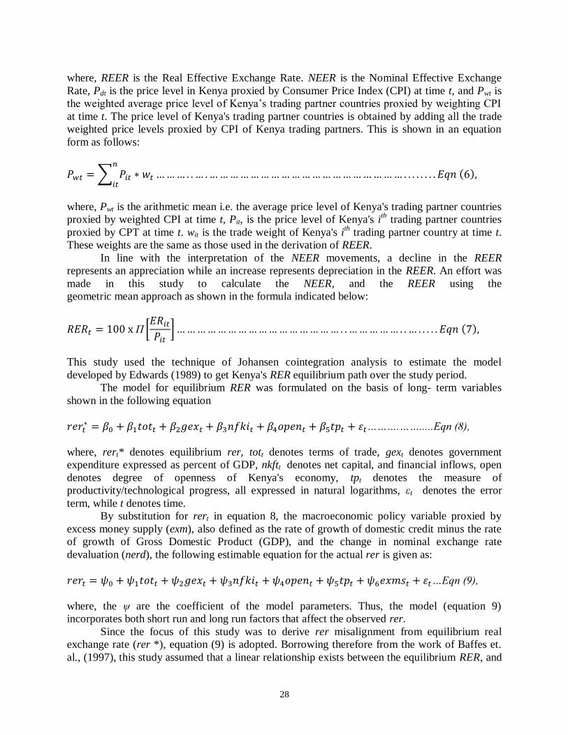
where, REER is the Real Effective Exchange Rate. NEER is the Nominal Effective Exchange

Rate, Pdt is the price level in Kenya proxied by Consumer Price Index (CPI) at time t, and Pwt is

the weighted average price level of Kenya’s trading partner countries proxied by weighting CPI

at time t. The price level of Kenya's trading partner countries is obtained by adding all the trade

weighted price levels proxied by CPI of Kenya trading partners. This is shown in an equation

form as follows:

where, Pwt is the arithmetic mean i.e. the average price level of Kenya's trading partner countries

proxied by weighted CPI at time t, Pit, is the price level of Kenya's ith

trading partner countries

proxied by CPT at time t. wit is the trade weight of Kenya's ith

trading partner country at time t.

These weights are the same as those used in the derivation of REER.

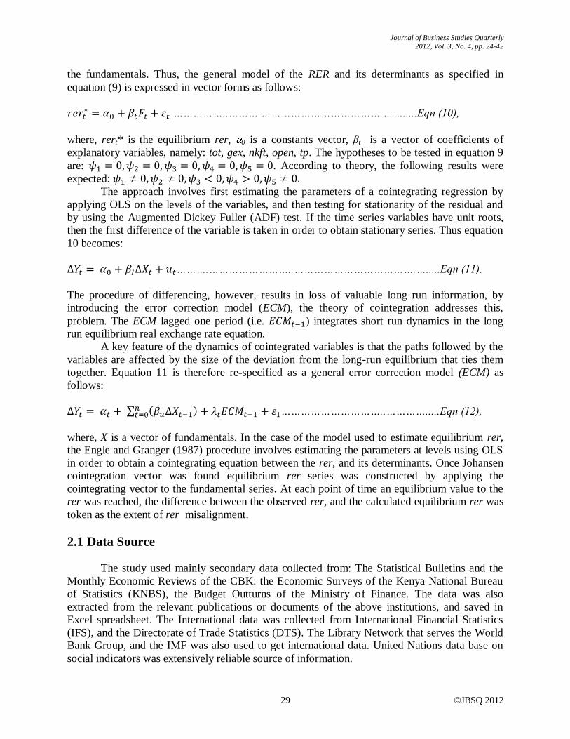
In line with the interpretation of the NEER movements, a decline in the REER

represents an appreciation while an increase represents depreciation in the REER. An effort was

made in this study to calculate the NEER, and the REER using the

geometric mean approach as shown in the formula indicated below:

This study used the technique of Johansen cointegration analysis to estimate the model

developed by Edwards (1989) to get Kenya's RER equilibrium path over the study period.

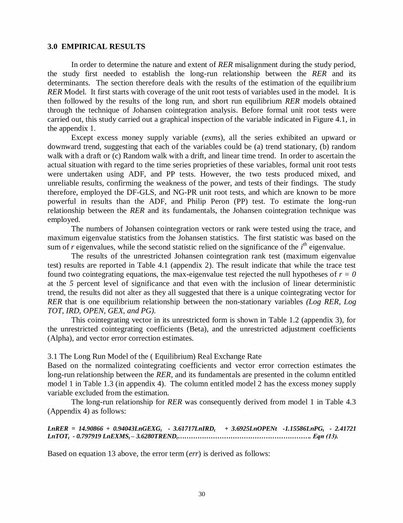
The model for equilibrium RER was formulated on the basis of long- term variables

shown in the following equation

……….…….....Eqn (8),

where, rert* denotes equilibrium rer, tott denotes terms of trade, gext denotes government

expenditure expressed as percent of GDP, nkftt denotes net capital, and financial inflows, open

denotes degree of openness of Kenya's economy, tpt denotes the measure of

productivity/technological progress, all expressed in natural logarithms, εt denotes the error

term, while t denotes time.

By substitution for rert in equation 8, the macroeconomic policy variable proxied by

excess money supply (exm), also defined as the rate of growth of domestic credit minus the rate

of growth of Gross Domestic Product (GDP), and the change in nominal exchange rate

devaluation (nerd), the following estimable equation for the actual rer is given as:

…Eqn (9),

where, the ψ are the coefficient of the model parameters. Thus, the model (equation 9)

incorporates both short run and long run factors that affect the observed rer.

Since the focus of this study was to derive rer misalignment from equilibrium real

exchange rate (rer *), equation (9) is adopted. Borrowing therefore from the work of Baffes et.

al., (1997), this study assumed that a linear relationship exists between the equilibrium RER, and

Journal of Business Studies Quarterly

2012, Vol. 3, No. 4, pp. 24-42

©JBSQ 2012 29

the fundamentals. Thus, the general model of the RER and its determinants as specified in

equation (9) is expressed in vector forms as follows:

……………..……….……………………………….…….....Eqn (10),

where, rert* is the equilibrium rer, 0 is a constants vector, βt is a vector of coefficients of

explanatory variables, namely: tot, gex, nkft, open, tp. The hypotheses to be tested in equation 9

are: . According to theory, the following results were

expected: The approach involves first estimating the parameters of a cointegrating regression by

applying OLS on the levels of the variables, and then testing for stationarity of the residual and

by using the Augmented Dickey Fuller (ADF) test. If the time series variables have unit roots,

then the first difference of the variable is taken in order to obtain stationary series. Thus equation

10 becomes:

……….……………………..……………………………….….....Eqn (11).

The procedure of differencing, however, results in loss of valuable long run information, by

introducing the error correction model (ECM), the theory of cointegration addresses this,

problem. The ECM lagged one period (i.e. ) integrates short run dynamics in the long

run equilibrium real exchange rate equation.

A key feature of the dynamics of cointegrated variables is that the paths followed by the

variables are affected by the size of the deviation from the long-run equilibrium that ties them

together. Equation 11 is therefore re-specified as a general error correction model (ECM) as

follows:

…………………………..………….....Eqn (12),

where, X is a vector of fundamentals. In the case of the model used to estimate equilibrium rer,

the Engle and Granger (1987) procedure involves estimating the parameters at levels using OLS

in order to obtain a cointegrating equation between the rer, and its determinants. Once Johansen

cointegration vector was found equilibrium rer series was constructed by applying the

cointegrating vector to the fundamental series. At each point of time an equilibrium value to the

rer was reached, the difference between the observed rer, and the calculated equilibrium rer was

token as the extent of rer misalignment.

2.1 Data Source

The study used mainly secondary data collected from: The Statistical Bulletins and the

Monthly Economic Reviews of the CBK: the Economic Surveys of the Kenya National Bureau

of Statistics (KNBS), the Budget Outturns of the Ministry of Finance. The data was also

extracted from the relevant publications or documents of the above institutions, and saved in

Excel spreadsheet. The International data was collected from International Financial Statistics

(IFS), and the Directorate of Trade Statistics (DTS). The Library Network that serves the World

Bank Group, and the IMF was also used to get international data. United Nations data base on

social indicators was extensively reliable source of information.

30

3.0 EMPIRICAL RESULTS

In order to determine the nature and extent of RER misalignment during the study period,

the study first needed to establish the long-run relationship between the RER and its

determinants. The section therefore deals with the results of the estimation of the equilibrium

RER Model. It first starts with coverage of the unit root tests of variables used in the model. It is

then followed by the results of the long run, and short run equilibrium RER models obtained

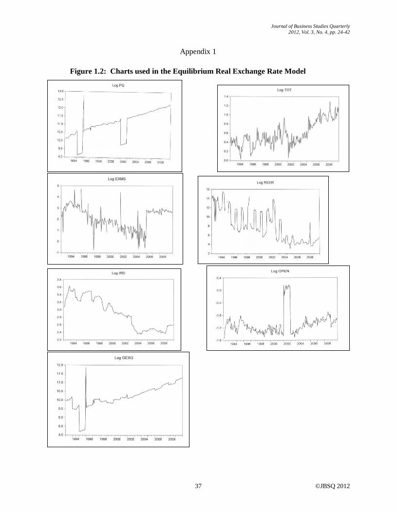
through the technique of Johansen cointegration analysis. Before formal unit root tests were

carried out, this study carried out a graphical inspection of the variable indicated in Figure 4.1, in

the appendix 1.

Except excess money supply variable (exms), all the series exhibited an upward or

downward trend, suggesting that each of the variables could be (a) trend stationary, (b) random

walk with a draft or (c) Random walk with a drift, and linear time trend. In order to ascertain the

actual situation with regard to the time series proprieties of these variables, formal unit root tests

were undertaken using ADF, and PP tests. However, the two tests produced mixed, and

unreliable results, confirming the weakness of the power, and tests of their findings. The study

therefore, employed the DF-GLS, and NG-PR unit root tests, and which are known to be more

powerful in results than the ADF, and Philip Peron (PP) test. To estimate the long-run

relationship between the RER and its fundamentals, the Johansen cointegration technique was

employed.

The numbers of Johansen cointegration vectors or rank were tested using the trace, and

maximum eigenvalue statistics from the Johansen statistics. The first statistic was based on the

sum of r eigenvalues, while the second statistic relied on the significance of the ith

eigenvalue.

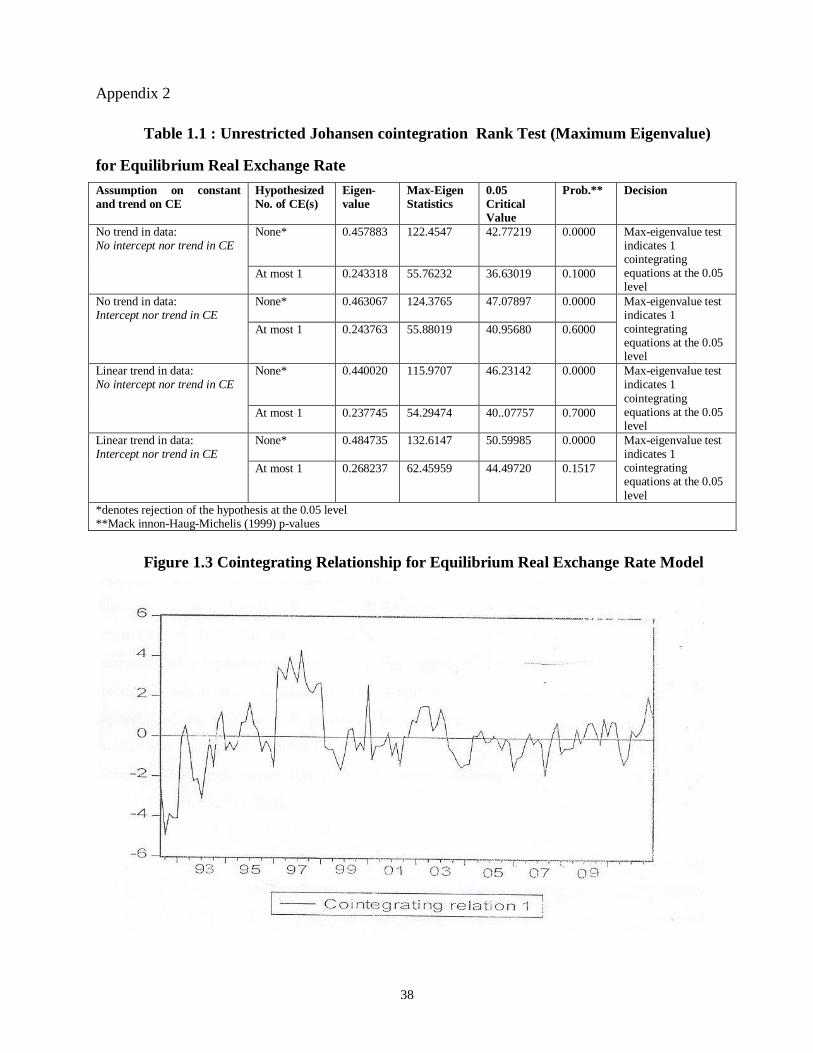
The results of the unrestricted Johansen cointegration rank test (maximum eigenvalue

test) results are reported in Table 4.1 (appendix 2). The result indicate that while the trace test

found two cointegrating equations, the max-eigenvalue test rejected the null hypotheses of r = 0

at the 5 percent level of significance and that even with the inclusion of linear deterministic

trend, the results did not alter as they all suggested that there is a unique cointegrating vector for

RER that is one equilibrium relationship between the non-stationary variables (Log RER, Log

TOT, IRD, OPEN, GEX, and PG).

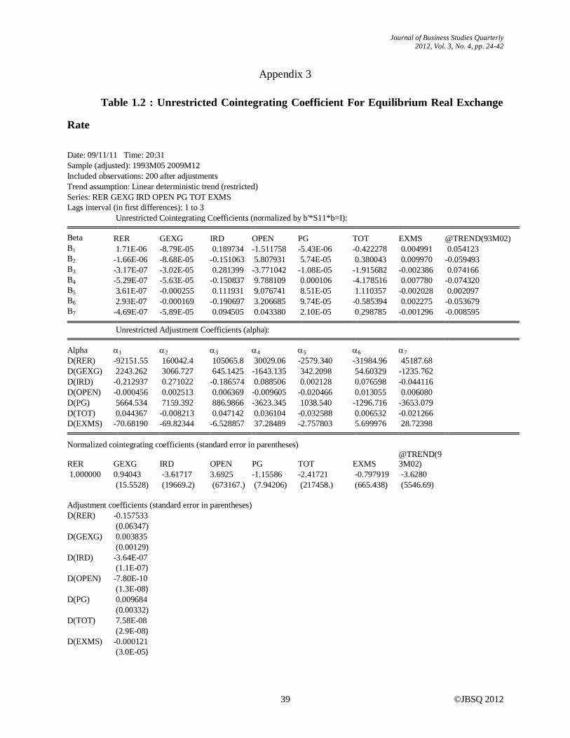
This cointegrating vector in its unrestricted form is shown in Table 1.2 (appendix 3), for

the unrestricted cointegrating coefficients (Beta), and the unrestricted adjustment coefficients

(Alpha), and vector error correction estimates.

3.1 The Long Run Model of the ( Equilibrium) Real Exchange Rate

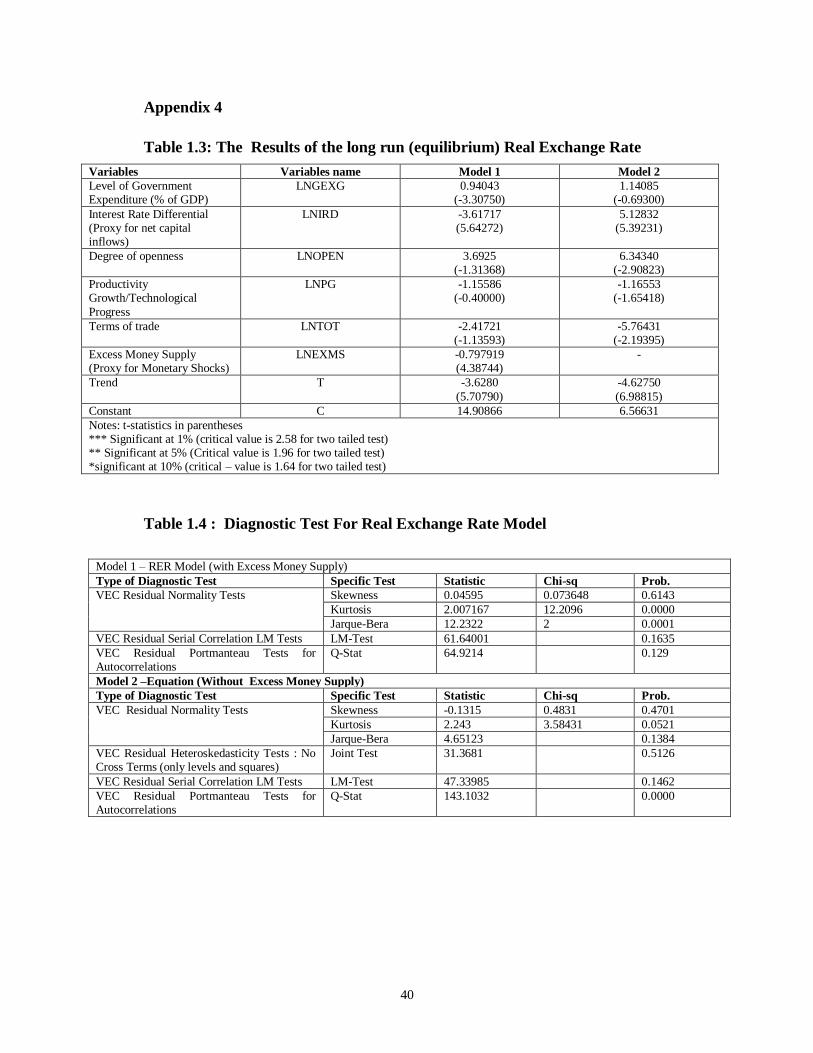
Based on the normalized cointegrating coefficients and vector error correction estimates the

long-run relationship between the RER, and its fundamentals are presented in the column entitled

model 1 in Table 1.3 (in appendix 4). The column entitled model 2 has the excess money supply

variable excluded from the estimation.

The long-run relationship for RER was consequently derived from model 1 in Table 4.3

(Appendix 4) as follows:

LnRER = 14.90866 + 0.94043LnGEXGt - 3.61717LnIRDt + 3.6925LnOPENt -1.15586LnPGt - 2.41721

LnTOTt - 0.797919 LnEXMSt – 3.6280TRENDt……………………………………………………. Eqn (13).

Based on equation 13 above, the error term (err) is derived as follows:

Journal of Business Studies Quarterly

2012, Vol. 3, No. 4, pp. 24-42

©JBSQ 2012 31

Err = LnRERt -14.90866 - 0.94043LnGEXGt + 3.61717LnIRDt + 3.6925LnOPENt + 1.15586LnPGt + 2.41721

LnTOTt + 0.797919 LnEXMSt + 3.6280TREND….……………………………...……….…Eqn(14).

The long-run relationship for RER from model 2, which excluded excess money supply variable,

is:

LnRER = 6.56631 + 1.14085LnGEXGt + 5.12832LnIRDt + 6.34340LnOPENt -1.16553LnPGt - 5.76432 LnTOTt

- 4.62750TRENDt …………………………………………………........................................Eqn (15).

The error term (err) of model 2, is thus:

Err = LnRER – 6.56631 – 1.14085 - 5.12832LnIRDt - 6.34340LnOPENt +1.16553LnPGt + 5.76432 LnTOTt +

4.62750TRENDt ……………………………………………….……………………….....Eqn (16).

3.2 The Short-Run Model of the Real Exchange Rate

According to the Granger representation theorem, a dynamic error –correction representation of

a set of data exists if a co integrating relationship exists among a set of 1 (1) series. Based on this

theorem, the study proceeded to find this representation for equilibrium RER by using the

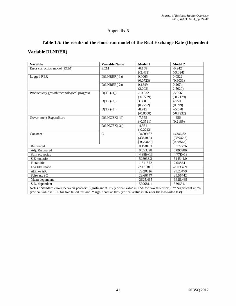
general-to-specific principle describe by Hendry et. al., (1984). Table 1.5 (appendix 5) shows the

parsimonious results.

Considering that each regress, and in Table 1.5 (Appendix 5) is cast in first-difference,

the empirical results suggest that the statistical fit of the models to the data is weak, as indicated

by the value of R2, which is 0.15 and 0.17 in models 1 and 2. The statistical appropriateness

fulfilled the condition of no serial correlation and homoscedasticity, but not the normality of

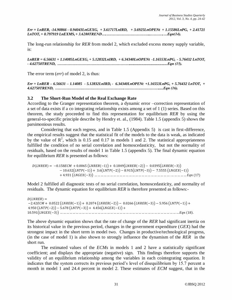
residuals, based on the results of model 1 in Table 1.5 (appendix 5). The final dynamic equation

for equilibrium RER is presented as follows:

Model 2 fulfilled all diagnostic tests of no serial correlation, homoscedasticity, and normality of

residuals. The dynamic equation for equilibrium RER is therefore presented as follows:-

The above dynamic equation shows that the rate of change of the RER had significant inertia on

its historical value in the previous period, changes in the government expenditure (GEX) had the

strongest impact in the short term in model two. Changes in productive/technological progress,

(in the case of model 1) is also shown to strongly influence the dynamism of the RER in the

short run.

The estimated values of the ECMs in models 1 and 2 have a statistically significant

coefficient; and displays the appropriate (negative) sign. This findings therefore supports the

validity of an equilibrium relationship among the variables in each cointegrating equation. It

indicates that the system corrects its previous period’s level of disequilibrium by 15.7 percent a

month in model 1 and 24.4 percent in model 2. These estimates of ECM suggest, that in the

32

absence of further shocks, the gap would be closed within a period of 6.3 months in model 1, and

4.1 months in model 2.

3.3 Real Exchange Rate Equilibrium, and Misalignment

The results of the estimated long run parameters shown in Table 1.3 (Appendix 4) were used to

calculate the equilibrium RER, and the degree of RER misalignment over the period 1993 -2009.

In particular, the long run relationship for RER from model 2, which excludes excess money

supply variable, was used due to its good results of diagnostic tests (Table 1.4- Appendix 4).

Thus, the equilibrium rers were obtained by using the actual values of fundamentals in the fitted

(i.e. estimated) model 2, whose results are shown in Table 1.3 (Appendix 4), and equation 15,

which we re-specify as:

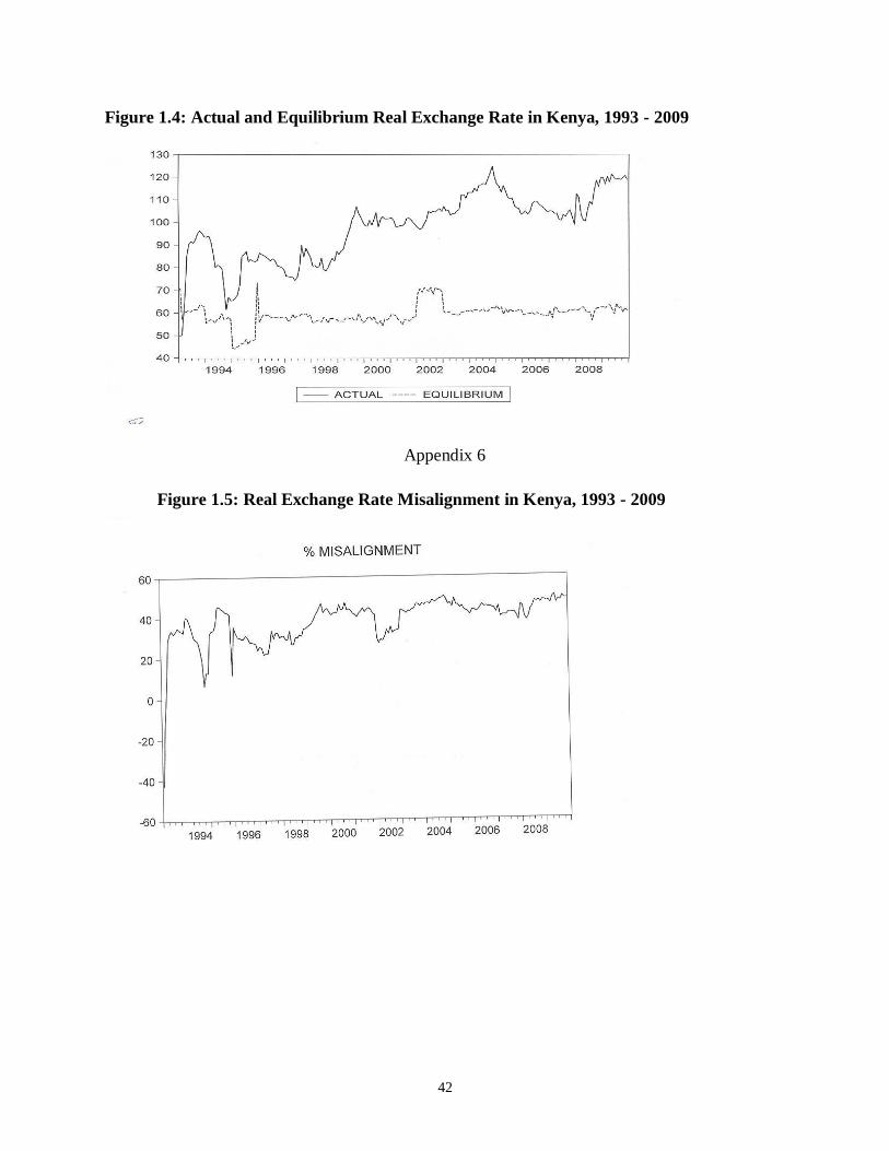
Figure 1.4 (Appendix 5) shows the profile of both the equilibrium RER and the actual RER over

the study period. Average deviations of the fitted values of RER form the actual ones were

expected to be zero by construction. Hence, deviations of actual indices form the fitted values

merely showed the short run RER misalignment. Such RER misalignment was expressed in

percentage form, and are shown in Figures 1.5 (Appendix 6). Based on these resulted, Kenya

lost international competitiveness when the value of RER misalignment was positive (i.e. was

overvalued), and gained international competiveness when the value of RER misalignment was

negative (i.e. was undervalued). When RER misalignment was zero, then Kenya did not lose

international competitiveness. Consequently economic growth deteriorates with RER over

valuation and improved with RER under valuation.

Figure 1.4 (Appendix 5) shows that the actual RER rate was more often than not above its

equilibrium value in the period between January 1993, and December 2009, implying that the

RER was generally overvalued during this period. The appreciation of the RER during this

period was attributed to significant appreciation in the NER brought about by capital, and

financial inflows owing to the then prevailing high interest rates regimes in government security

markets. The appreciation pressures observed in the trend of RER over this period could also be

attributed to significant improvements in the terms of trade as a result of the coffee boom, and

the corresponding increased in commodity prices.

These results are mainly attributed to developments in some of the fundamentals. Over

these periods, there was an increase in the degree of openness variable, and this is assumed to be

due to decline in customs tariff rates, which led to a fall in the domestic prices of importable.

This led to high, demand of foreign currency (to take advantage of cheap imports), and

less demand for domestic currency. Hence the increase in the degree of openness that led to the

depreciation of the equilibrium RER. The RER was, however, overvalued in the period, implying

also deterioration in the country’s international competitiveness hence deterioration of economic

growth, albeit marginal. It is also a reflection of relatively high interest rates domestically that

led to capital and financial inflows, hence the appreciation of the RER.

Overall, figure 1.5 (Appendix 6) shows that, between 1993 and 2009, Kenya’s RER

misalignment generally exhibited a appreciating trend, implying that in general, the country’s

international competitiveness deteriorated over the study period.

Journal of Business Studies Quarterly

2012, Vol. 3, No. 4, pp. 24-42

©JBSQ 2012 33

4.0 CONCLUSIONS AND DISCUSSIONS

One of the main objectives of this study was to estimate Kenya’s equilibrium RER path,

determine the degree of RER misalignment between the observed, and equilibrium RER.

Drawing heavily from the works of, among others, Edwards (1989), and Baffes et. al., (1997),

the study employed the technique of Johansen cointegration analysis based on a single equation

approach to establish the equilibrium RER over the period 1993 to 2009. The deviations of actual

RERs from the equilibrium RER path, which represent RER misalignment, was then calculated.

The result show that during the study period, the actual RER rate was more often than not

above its equilibrium value in the period between June 1993 and December 2009, implying that

the RER was generally overvalued. Overall, however, Kenya’s RER generally exhibited a

appreciating trend, implying that in general, the country’s international competitiveness

deteriorated over the study period.

The conclusion drawn from these results is that the adoption of the floating exchange rate

regime has not achieved the intended purpose for which it was established, namely to reduce

RER misalignment, and in particular RER overvaluation. Although declining, and generally

exhibiting an appreciating trend, RER misalignment continued to hamper the country’s economic

growth. Results similar to this study were reported by various authors, mostly dealing with

developing countries.

The study by Elbadawi, and Soto (1997) focused on capital flows, and long-term

equilibrium RERs in Chile, and found that under a pegged NER expansionary fiscal, and

monetary policy tended to cause persistent RER overvaluation. Similar conclusions were drawn

by the study of Norman et. al., (1997), who examined the degree of misalignment of the RER in

Argentina, Brazil, Chile, Colombia, Mexico, Peru, the United States, and Venezuela. The study

by Zalduendo (2006) also found that parallel market rate of Venezuela was 15 percent more-

appreciated than its equilibrium rate (but still below the official rate), and that the -speed of

adjustment to this equilibrium was much higher.

The studies carried out in Africa were: Baffes, et. al., (1997), Aron et. al., (1997),

Mongardini (1998), Nabli and Veganzones-Varoudakis (2002), MacDonald and Ricci (2003),

Mathisen (2003), Koranchclian (2005), and Limi (2006), majority of these studies used the

technique of Johansen cointegration to estimate the equilibrium RER path, and derive the degree

of RER misalignment in the respective countries. A number of them also established that

countries were characterized by a significant overvaluation of their currency, and that this

overvaluation had a cost for the region in terms of export competitiveness, particularly, to

manufactured goods. Most of the results also showed that RER overvaluation had declined in the

1990s and beyond.

The study by Ranki (2002) also derived equilibr ium RERs, and calculated the

misalignment by subtracting the equilibrium RER from the actual RER. The results showed

that the deviations from the equ i l ibr ium RER have been transitory and surpr is ing ly small

(15% at the highest). These results were supported by a study by Beguna (2002), who

estimated the equilibrium RER for Latvia. Based on the Fundamental Equilibrium Exchange

Rates (FEER) methodology, the study found that on a yearly basis, the RER in Latvian was

overvalued by 2 percent.

The study by Ghura, and Grennes (1993) found that Edwards (1989) model of RER

determination performed well for Kenya, and the region at large. Black market premia tended to

show a greater degree of misalignment in RER than alternative measures. The study observed that

34

misalignment of the RER acted as an implicit tax on exports, and that as the RER gets more

overvalued, the profitability of producing exportable goods falls, and hence less was produced.

Elbadawi and Soto (1997) estimated the long run cointegrated equilibrium of the RER, and

a set of fundamentals consistent with internal, and external balances for seven developing

countries including 4 countries from Sub-Saharan Africa (SSA) for the period 1960-93. The SSA

countries were: CoteD'Ivoire, Mali, Kenya, and Ghana. Both Cote D’lvoire and Mali belonged

to the fixed exchange rate economies of Communaute Financiere Africanised (CFA) Monetary

Union while Kenya and Ghana represented the other flexible exchange rate economies covered

by the study.

In particular, the results indicated that the Kenya shilling was generally overvalued during the

study period 1960-93.

Bleaney, and Greenaway (2001) estimated investment, and growth equations on a

reasonably sized panel of annual data from 14 sub-Saharan African countries (including Kenya)

from 1980 to 1995. Both growth and investment were higher when the, terms of trade were

more favorable, and the RER was less overvalued. The most striking feature of the sample was

that all countries had experienced considerable RER depreciation by more than 4% per annum

on average.

Finally, the study by Maturu (2002), examined the RER behaviour for Kenya using

quarterly data drawn for the period 1980:1998:4 using Johansen cointegration analysis. The

results showed that a linear relationship binding together the RER, and its fundamentals existed

in Kenya during the study period. The study show Kenya RER was overvalued

The study by Kiptoo (2007), focused on RER volatility and misalignment on international

trade and investment. The study found out that RER was undervalued, and that RER volatility

and misalignment has a negative and significance impact on trade and investment during the

study period 1993 to 2003.

Journal of Business Studies Quarterly

2012, Vol. 3, No. 4, pp. 24-42

©JBSQ 2012 35

REFERENCES

Aron, J., Elbadawi 1. & Khan, B., 1997. Determinants of the Real Exchange Rate in South

Africa, Centre for the Study of African Economies Working Paper Series, No. 16,

University of Oxford.

Baffes, J.B., Elbadawi, LA., & O'ConneIlS. A., 1997. Single-Equation Estimation of the

Equilibrium Exchange Rate, A World Bank Policy - Research Working Paper in

http://www.worldbank.org/html/dec/Publications/Workpapers/WPSI800series/wps1800/

wps1800.pdf

Bleaney, M. & Greenaway, D., 2001. The Impact of Terms of Trade and Real Exchange Rate

Volatility on Investment and Growth in Sub-Saharan Africa, Journal of

Development Economics, Vol. 65, pp. 491-500 www.elsevier.comrlocatereconbase.

Copeland, L. S., 1989. Exchange Rates and International Finance, University of Manchester

Institute, United Kingdom pp. 41-75.

Edwards, S., 1989. Exchange Rate Misalignment in developing Countries, National Bureau of

Economic Research (NBER) Working Paper Series, No. 2950, April, Oxford University

Press.

Elbadawi, I. & Soto, R., 1997. Real Exchange Rates and Macroeconomic Adjustment in

Sub-Saharan Africa and Other Developing Countries, Journal of African Economies, Vol.

6(3), pp. 74-120.

Engle, R.F. & Granger, C.W.G., 1987. Co-Integration and Error Correction: Representation,

Estimation, and Testing, Econometrica, Vol. 55, No 2.

Ghura, D. & Grennes T.J., 1993. The Real Exchange Rate and Macroeconomics Performance in

Africa, Journal of Development Economics, Vol. 32: 155-174, North-Holland.

Gylfason, T., 2002. The Real Exchange Rate Always Floats, center for Economic Policy

Research (CEPR) Discussion Paper Series No. 3376, London.

Hendry D. Pagan, A & Sargan, J.D., 1984. Dynamic Specification, in Handbook of

Econometrics, Vol. 1, (EDS, Griliges, Z. and Intrilagor, M.), Amsterderm, North

Holland.

Kiptoo C., 2007. Real Exchange Rate Volatility, and misalignment in Kenya,1993-2003 ,

Assessment of its impact on International Trade, and investments, unpublished Ph.D

Thesis, University of Nairobi .

Koranchelian, T., 2005. The Equilibrium Real Exchange Rate in a Commodity Exporting

Country: Algeria's Experience, IMF Working Paper Series, WP/051135, IMF,

Washington DC, 20431, USA.

Limi, A., 2006. Exchange Rate Misalignment: An Application of the Behavioural Equilibrium

Exchange Rate (BEER) to Botswana, IMF Working Paper, WP/061140, IMF,

Washington DC, 20431.

Lothian, J.R. & Taylor, M.P., 1997. Real Exchange Rate behaviour, Journal of International

Money and Finance, Vol. 116, No. 6, pp.945-954.

36

MacDonald R. & Ricci, L. 2003. Estimation of Equilibrium Real Exchange Rate for South

Africa, IMF Working Paper NO. WP/03/44, IMF, Washington DC, 20431.

Mathisen, J. 2003. Estimation of Equilibrium~ Real Exchange Rate for Malawi, IMF Working

Paper No. WP/031104, IMF, Washington D.C., 20431, USA.

Maturu, B.O. 2002. Modeling the Real Exchange Rate for Kenya, 1980-1998, Unpublished Ph.d

Thesis, Jomo Kenyatta University of Agriculture and Technology.

Mongardini, J. 1998. Estimating Egypt's Equilibrium Real Exchange Rate, IMF Working Paper

No. WP/98/5, IMF, Washington D.C. 20431,USA.

Nabli, M.K. & Veganzones-Varoudakis M. 2002. Exchange Rate Regime and Competitiveness .

of Manufactured Exports: The Case of MENA Countries,

http://lnweb18.worldbank.org/mna/mena.nsf/Attachments/Nabli-

Veganzones/$File/Nabli-Veganzones.pdf

Ndung’u, N.S. 1999. Monetary and Exchange Rate Policy in Kenya, AERC, Research, Paper

No. 94, Nairobi, Kenya.

Norman, L., Humberto, L. J. & Fernando B. 1997. Misalignment and Fundamentals: Equilibrium

Exchange Rates in Seven Latin American Countries, World Bank, Policy Research

Department, Washington, DC. http://wbln0018.worldbank.org/Research/workpapers.nsf.

Ranki, S. 2002. The Real Exchange Rate as an Indicator of Baltic Competitiveness,

Bimonthly Review, Institute of Economies in Transition, Bank of Finland.

Sifunjo, E. K 2011. Chaos and Non-linear Dynamical Approaches to Predicting Exchange Rates

in Kenya, Unplished PhD Thesis University of Nairobi.

Were, M., Geda, A., Karingi, S. and Njuguna, S.N. (2001). Kenya’s Exchange rate Movement in

a Liberalised Environment:, An Empirical Analysis, The Kenya Institute for Public

Policy Research and Analysis (KIPPRA), Discussion paper Series No. 10, Nairobi,

Kenya.

Zalduendo, J. 2006. Determinants of Venezuela's Equilibrium Real Exchange, IMF

Working Paper Series, No. WP/06174, IMF, Washington DC, 20431.

Journal of Business Studies Quarterly

2012, Vol. 3, No. 4, pp. 24-42

©JBSQ 2012 37

Appendix 1

Figure 1.2: Charts used in the Equilibrium Real Exchange Rate Model

38

Appendix 2

Table 1.1 : Unrestricted Johansen cointegration Rank Test (Maximum Eigenvalue)

for Equilibrium Real Exchange Rate

Assumption on constant

and trend on CE

Hypothesized

No. of CE(s)

Eigen-

value

Max-Eigen

Statistics

0.05

Critical

Value

Prob.** Decision

No trend in data: No intercept nor trend in CE

None* 0.457883 122.4547 42.77219 0.0000

Max-eigenvalue test indicates 1 cointegrating equations at the 0.05 level

At most 1 0.243318 55.76232 36.63019 0.1000

No trend in data: Intercept nor trend in CE

None* 0.463067 124.3765 47.07897 0.0000

Max-eigenvalue test indicates 1 cointegrating equations at the 0.05 level

At most 1 0.243763 55.88019 40.95680 0.6000

Linear trend in data: No intercept nor trend in CE

None* 0.440020 115.9707 46.23142 0.0000

Max-eigenvalue test indicates 1

cointegrating equations at the 0.05 level

At most 1 0.237745 54.29474 40..07757 0.7000

Linear trend in data: Intercept nor trend in CE

None*

0.484735 132.6147 50.59985 0.0000 Max-eigenvalue test indicates 1 cointegrating equations at the 0.05

level

At most 1 0.268237 62.45959 44.49720 0.1517

*denotes rejection of the hypothesis at the 0.05 level **Mack innon-Haug-Michelis (1999) p-values

Figure 1.3 Cointegrating Relationship for Equilibrium Real Exchange Rate Model

Journal of Business Studies Quarterly

2012, Vol. 3, No. 4, pp. 24-42

©JBSQ 2012 39

Appendix 3

Table 1.2 : Unrestricted Cointegrating Coefficient For Equilibrium Real Exchange

Rate

Date: 09/11/11 Time: 20:31

Sample (adjusted): 1993M05 2009M12

Included observations: 200 after adjustments

Trend assumption: Linear deterministic trend (restricted)

Series: RER GEXG IRD OPEN PG TOT EXMS

Lags interval (in first differences): 1 to 3

Unrestricted Cointegrating Coefficients (normalized by b'*S11*b=I): Beta RER GEXG IRD OPEN PG TOT EXMS @TREND(93M02) B1 1.71E-06 -8.79E-05 0.189734 -1.511758 -5.43E-06 -0.422278 0.004991 0.054123 B2 -1.66E-06 -8.68E-05 -0.151063 5.807931 5.74E-05 0.380043 0.009970 -0.059493 B3 -3.17E-07 -3.02E-05 0.281399 -3.771042 -1.08E-05 -1.915682 -0.002386 0.074166 B4 -5.29E-07 -5.63E-05 -0.150837 9.788109 0.000106 -4.178516 0.007780 -0.074320

B5 3.61E-07 -0.000255 0.111931 9.076741 8.51E-05 1.110357 -0.002028 0.002097 B6 2.93E-07 -0.000169 -0.190697 3.206685 9.74E-05 -0.585394 0.002275 -0.053679 B7 -4.69E-07 -5.89E-05 0.094505 0.043380 2.10E-05 0.298785 -0.001296 -0.008595 Unrestricted Adjustment Coefficients (alpha): Alpha 1 2 3 4 5 6 7

D(RER) -92151.55 160042.4 105065.8 30029.06 -2579.340 -31984.96 45187.68

D(GEXG) 2243.262 3066.727 645.1425 -1643.135 342.2098 54.60329 -1235.762

D(IRD) -0.212937 0.271022 -0.186574 0.088506 0.002128 0.076598 -0.044116

D(OPEN) -0.000456 0.002513 0.006369 -0.009605 -0.020466 0.013055 0.006080

D(PG) 5664.534 7159.392 886.9866 -3623.345 1038.540 -1296.716 -3653.079

D(TOT) 0.044367 -0.008213 0.047142 0.036104 -0.032588 0.006532 -0.021266

D(EXMS) -70.68190 -69.82344 -6.528857 37.28489 -2.757803 5.699976 28.72398

Normalized cointegrating coefficients (standard error in parentheses)

RER GEXG IRD OPEN PG TOT EXMS @TREND(93M02)

1.000000 0.94043 -3.61717 3.6925 -1.15586 -2.41721 -0.797919 -3.6280

(15.5528) (19669.2) (673167.) (7.94206) (217458.) (665.438) (5546.69)

Adjustment coefficients (standard error in parentheses)

D(RER) -0.157533

(0.06347)

D(GEXG) 0.003835

(0.00129)

D(IRD) -3.64E-07

(1.1E-07)

D(OPEN) -7.80E-10

(1.3E-08)

D(PG) 0.009684

(0.00332)

D(TOT) 7.58E-08

(2.9E-08)

D(EXMS) -0.000121

(3.0E-05)

40

Appendix 4

Table 1.3: The Results of the long run (equilibrium) Real Exchange Rate

Variables Variables name Model 1 Model 2

Level of Government Expenditure (% of GDP)

LNGEXG 0.94043 (-3.30750)

1.14085 (-0.69300)

Interest Rate Differential (Proxy for net capital inflows)

LNIRD -3.61717 (5.64272)

5.12832 (5.39231)

Degree of openness LNOPEN 3.6925 (-1.31368)

6.34340 (-2.90823)

Productivity Growth/Technological

Progress

LNPG -1.15586 (-0.40000)

-1.16553 (-1.65418)

Terms of trade LNTOT -2.41721 (-1.13593)

-5.76431 (-2.19395)

Excess Money Supply (Proxy for Monetary Shocks)

LNEXMS -0.797919 (4.38744)

-

Trend T -3.6280

(5.70790)

-4.62750

(6.98815)

Constant C 14.90866 6.56631

Notes: t-statistics in parentheses *** Significant at 1% (critical value is 2.58 for two tailed test) ** Significant at 5% (Critical value is 1.96 for two tailed test) *significant at 10% (critical – value is 1.64 for two tailed test)

Table 1.4 : Diagnostic Test For Real Exchange Rate Model

Model 1 – RER Model (with Excess Money Supply)

Type of Diagnostic Test Specific Test Statistic Chi-sq Prob.

VEC Residual Normality Tests Skewness 0.04595 0.073648 0.6143

Kurtosis 2.007167 12.2096 0.0000

Jarque-Bera 12.2322 2 0.0001

VEC Residual Serial Correlation LM Tests LM-Test 61.64001 0.1635

VEC Residual Portmanteau Tests for Autocorrelations

Q-Stat 64.9214 0.129

Model 2 –Equation (Without Excess Money Supply)

Type of Diagnostic Test Specific Test Statistic Chi-sq Prob.

VEC Residual Normality Tests Skewness -0.1315 0.4831 0.4701

Kurtosis 2.243 3.58431 0.0521

Jarque-Bera 4.65123 0.1384

VEC Residual Heteroskedasticity Tests : No Cross Terms (only levels and squares)

Joint Test 31.3681 0.5126

VEC Residual Serial Correlation LM Tests LM-Test 47.33985 0.1462

VEC Residual Portmanteau Tests for Autocorrelations

Q-Stat 143.1032 0.0000

Journal of Business Studies Quarterly

2012, Vol. 3, No. 4, pp. 24-42

©JBSQ 2012 41

Appendix 5

Table 1.5: the results of the short-run model of the Real Exchange Rate (Dependent

Variable DLNRER)

Variable Variable Name Model 1 Model 2

Error correction model (ECM) ECM -0.158 (-2.482)

-0.242 (-3.324)

Lagged RER D(LNRER(-1)) 0.0065 (0.0723)

0.0522 (0.6031)

D(LNRER(-2)) 0.1849 (2.002)

0.2074 2.5029)

Productivity growth/technological progress D(TP (-1)) -10.632 (-0.7729)

-5.956 (-0.7179)

D(TP (-2)) 3.600 (0.2752)

4.950 (0.599)

D(TP (-3)) -8.915 (-0.8588)

--5.678 (-0.7232)

Government Expenditure D(LNGEX(-1)) -7.555 (-0.3511)

4.456 (0.2189)

D(LNGEX(-3)) -4.931 (-0.2243)

Constant C 34809.67 (43610.3) [ 0.79820]

14246.82 (36942.2) [0.38565]

R-squared 0.158163 0.177776

Adj. R-squared 0.053528 0.090986

Sum sq. resids 4.88E+13 4.77E+13

S.E. equation 525038.3 514544.0

F-statistic 1.511572 2.048341

Log likelihood -2905.816 -2903.459

Akaike AIC 29.28816 29.23459

Schwarz SC 29.66747 29.56442

Mean dependent -3625.465 -3625.465

S.D. dependent 539681.1 539681.1

Notes : Standard errors between parents” Significant at 1% (critical value is 2.58 for two tailed test), ** Significant at 5% (critical value is 1.96 for two tailed test and * significant at 10% (critical-value is 16.4 for the two tailed test)

42

Figure 1.4: Actual and Equilibrium Real Exchange Rate in Kenya, 1993 - 2009

Appendix 6

Figure 1.5: Real Exchange Rate Misalignment in Kenya, 1993 - 2009