Report Systems Comparison

Field Measurements, Evaluation and Comparison of Supermarket Refrigeration Systems

Final Report

Author: Pavel Makhnatch

Project leader / supervisor: Jörgen Rogstam

January 2011

Stockholm - Sweden

ABSTRACT

Current paper summarizes partial results of the project initiated by Sveriges Energi- & Kylcentrum in Katrineholm and co-financed by the Swedish energy agency. The project evaluates the potential of refrigeration systems using carbon dioxide in supermarket refrigeration.

This report includes the description and analysis of a number of supermarkets using different cooling systems such as CO2 transcritical chiller unit, CO2 transcritical freezer unit, CO2 transcritical booster unit, R404A/CO2 cascade unit, etc.

The collected data cover a long period (varies from supermarket to supermarket and is more than a year of constant analysis in some cases). The data collected has been summarized and evaluated in order to reveal the opportunities for improving the design and regulation of different refrigeration systems.

CO2 fluid as refrigerant for supermarket‟s refrigeration systems has been studied in detail and compared to the conventional HFC-based refrigeration solutions.

CONTENTS

Abstract ................................................................................................................................ 2

Contents ............................................................................................................................... 3

List of Figures ....................................................................................................................... 5

List of tables ......................................................................................................................... 9

Nomenclature ..................................................................................................................... 10

1. Introduction ................................................................................................................. 13

1.1 Description of the project ....................................................................................... 13

1.2 Methodology and Objectives ................................................................................. 14

2. Refrigeration solutions................................................................................................. 15

2.1 Indirect systems .................................................................................................... 15

2.2 Cascade DX systems ............................................................................................ 16

2.3 Transcritical DX systems ....................................................................................... 17

3. Measurements and Evaluation Methods ..................................................................... 18

3.1 Pressure and temperature. .................................................................................... 18

3.2 Electrical power consumption ................................................................................ 20

3.3 Mass flow .............................................................................................................. 23

3.4 COP calculation .................................................................................................... 28

4. Systems‟ descriptions and performance analysis ........................................................ 31

4.1 Supermarket refrigeration system RS1 ................................................................. 31

4.1.1 RS1 description .............................................................................................. 31

4.1.2 RS1 analysis ................................................................................................... 33


4.2.1 RS2 description .............................................................................................. 36

4.2.2 RS2 analysis ................................................................................................... 38


4.3.1 RS3 description .............................................................................................. 42

4.3.2 RS3 analysis ................................................................................................... 43

4.4 Supermarket with transcritical system TR1 ........................................................... 44

4.4.1 TR1 description ............................................................................................... 44

4.4.2 TR1 analysis ................................................................................................... 47


4.5.1 TR2 description ............................................................................................... 50

4.5.2 TR2 analysis ................................................................................................... 52


4.6.1 TR3 description ............................................................................................... 55

4.6.2 TR3 analysis ................................................................................................... 57


4.7.1 TR4 description ............................................................................................... 61

4.7.2 TR4 analysis ................................................................................................... 66


4.8.1 TR5 description ............................................................................................... 69

4.8.2 TR5 analysis ................................................................................................... 69

4.9 Supermarket with cascade system CC1 ................................................................ 72

4.9.1 CC1 description .............................................................................................. 72

4.9.2 CC1 analysis................................................................................................... 74

4.10 Supermarket with cascade system CC2 ............................................................ 76

4.10.1 CC2 description ........................................................................................... 76

4.10.2 Overall system description .......................................................................... 76

4.10.3 CC2 analysis ............................................................................................... 79

4.11 Supermarket with cascade system CC3 ............................................................ 87

4.11.1 CC3 description ........................................................................................... 87

4.11.2 CC3 analysis ............................................................................................... 92

4.12 Pump circulation system PC1 ............................................................................ 92

4.12.1 PC1 description ........................................................................................... 92

4.12.2 PC1 analysis ............................................................................................... 95

5. Refrigeration systems comparison .............................................................................. 96

6. Parasitic energy loads in refrigiration systems and their influence on total system‟s performance ..................................................................................................................... 104

7. Conclusion ................................................................................................................ 108

8. Bibliography .............................................................................................................. 109

LIST OF FIGURES

Figure 2.1: Secondary fluid systems with phase change (Girotto, 2005). ........................... 15 Figure 2.2: Direct expansion system in cascade (Girotto, 2005). ....................................... 16 Figure 2.3: Simplified trans-critical CO2 system with two-stage compression and inter-cooling for the low temperature unit and single stage compression for the medium temperature unit (left) and Ph diagramm for one stage (right). ........................................... 17

Figure 3.1: Schematic of a CO2 Transcritical Supermarket with the pressure and temperature measurement points. ...................................................................................... 19 Figure 3.2: ViSi+ interface for referent system ................................................................... 19 Figure 3.3: Data normalisation software user interface ...................................................... 20 Figure 3.4: Compressor electrical power measured for one day in July 2008 (01.07.08) in TR1 Supermarket. .............................................................................................................. 21 Figure 3.5: Compressor‟s electrical power consumption as a function of the pressure ratio for Bitzer compressors in CC1 supermarket. ...................................................................... 22 Figure 3.6: Electrical power consumption, comparison with the two methods for a single stage CO2 system during the whole year 2008, KA1 unit in the TR1 Supermarket. ........... 23 Figure 3.7: Volumetric efficiency based on compressor data for three CO2 compressors .. 24 Figure 3.8: Mass flow of CO2 in the freezer system FA1 during one day of July 2008 in the TR1 supermarket ................................................................................................................ 25 Figure 3.9: Mass flow of CO2 in a transcritical system for different mass flow measurement method ............................................................................................................................... 26 Figure 3.10:COP of a CO2 transcritical system for different mass flow measurement method ............................................................................................................................... 27 Figure 4.1: Simplified circuit of the reference refrigeration systems ................................... 31

Figure 4.2: System RS1: main parameters for the medium temperature side during the observation period .............................................................................................................. 33 Figure 4.3: System RS1: Main parameters for the low temperature side during the observation period .............................................................................................................. 34 Figure 4.4: System RS1: condensing temperature for the medium and low temperature side, outdoor temperature, and the differential of temperature between the condensing temperature and the outdoor temperature. ......................................................................... 35 Figure 4.5: System RS1: Coefficient of performance for the chiller and the freezer ........... 35

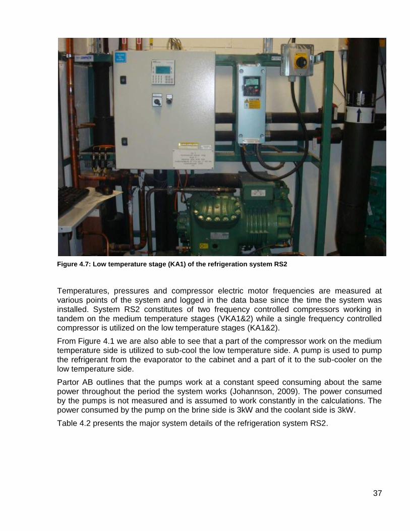
Figure 4.6: Medium temperature stage (VKA1) of the refrigeration system RS2 ................ 36 Figure 4.7: Low temperature stage (KA1) of the refrigeration system RS2 ........................ 37

Figure 4.8: System RS2: condensing temperature of each units and outdoor temperature during the observation period. ............................................................................................ 39 Figure 4.9: System RS2: cooling capacity and electrical consumption for low and medium temperature units during the observation period. ............................................................... 40 Figure 4.10: System RS2: average of the subcooling for both freezers units, evaporating temperature for the low and the medium temperature side, and the outdoor temperature during the observation period ............................................................................................. 40 Figure 4.11: System RS2: COP for the chillers units and the freezers units during the observation period. ............................................................................................................. 41 Figure 4.12: System RS3: cooling capacity and electrical consumption for the medium and the low temperature units. .................................................................................................. 43

Figure 4.13: System RS3: subcooling capacity and evaporating temperature of chillers and freezers during the observation period. .............................................................................. 44 Figure 4.14: Refrigiration unit in TR1 Supermarket ............................................................ 45 Figure 4.15: Schematic diagram of the TR1 system ........................................................... 46

Figure 4.16: Cooling capacity of one medium temperature unit (KA1) and one low temperature unit (FA1) during the years 2008 – 2009 ........................................................ 47 Figure 4.17: Compressors electrical power consumption for one medium temperature unit (KA1) and one low temperature unit (FA1) during the years 2008 - 2009 .......................... 48 Figure 4.18: COP function of coolant temperature for medium temperature units and low temperature units, measures for TR1 supermarket during 2008. ....................................... 49 Figure 4.19: COP for each units during the whole testing period for the TR1 supermarket. ........................................................................................................................................... 49 Figure 4.20: Booster unit in TR2 Supermarket ................................................................... 50

Figure 4.21: Schematic diagram of the TR2 system ........................................................... 51 Figure 4.22: Different parameters plots for the KAFA1 unit during the whole period of study in the TR2 supermarket ...................................................................................................... 52

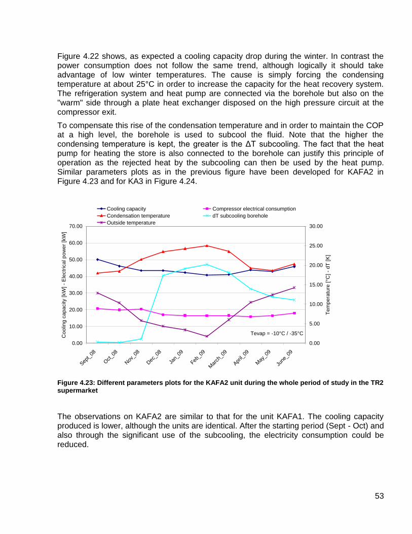
Figure 4.23: Different parameters plots for the KAFA2 unit during the whole period of study in the TR2 supermarket ...................................................................................................... 53

Figure 4.24: Different parameters plots for the KA3 unit during the whole period of study in the TR2 supermarket .......................................................................................................... 54

Figure 4.25: COP for each units during the whole testing period for the TR2 supermarket. ........................................................................................................................................... 55 Figure 4.26: Schematic diagram of the TR3 system unit 1 (KA/FA1) ................................. 56

Figure 4.27: Different parameters plots for the KA/FA1 unit during the whole period of study in the TR3 supermarket ...................................................................................................... 57 Figure 4.28: Different parameters plots for the KA/FA2 unit during the whole period of study in the TR3 supermarket ...................................................................................................... 58

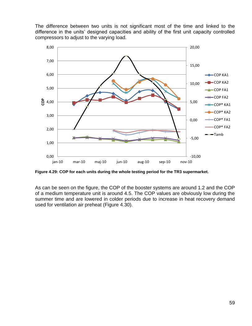
Figure 4.29: COP for each units during the whole testing period for the TR3 supermarket. ........................................................................................................................................... 59

Figure 4.30: Schematic diagram of the TR3 system heat recovery unit ............................. 60 Figure 4.31: Refrigiration system TR 3 heat recovery performance ................................... 61 Figure 4.32: Combine chiller and freezer unit for system TR4............................................ 62

Figure 4.33: Freezer unit (left) and chiller unit (right) for system TR5. ............................... 63

Figure 4.34: System schematic for TR4 and TR5 with important components and measurement points. .......................................................................................................... 64 Figure 4.35: Simplified P-h diagram for TR4 and TR5 during trans-critical operation. ........ 66

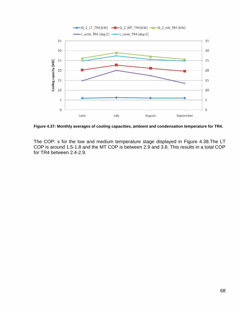
Figure 4.36: Monthly averages of LT, MT and total power consumption and outdoor temperature for TR4. .......................................................................................................... 67 Figure 4.37: Monthly averages of cooling capacities, ambient and condensation temperature for TR4. .......................................................................................................... 68

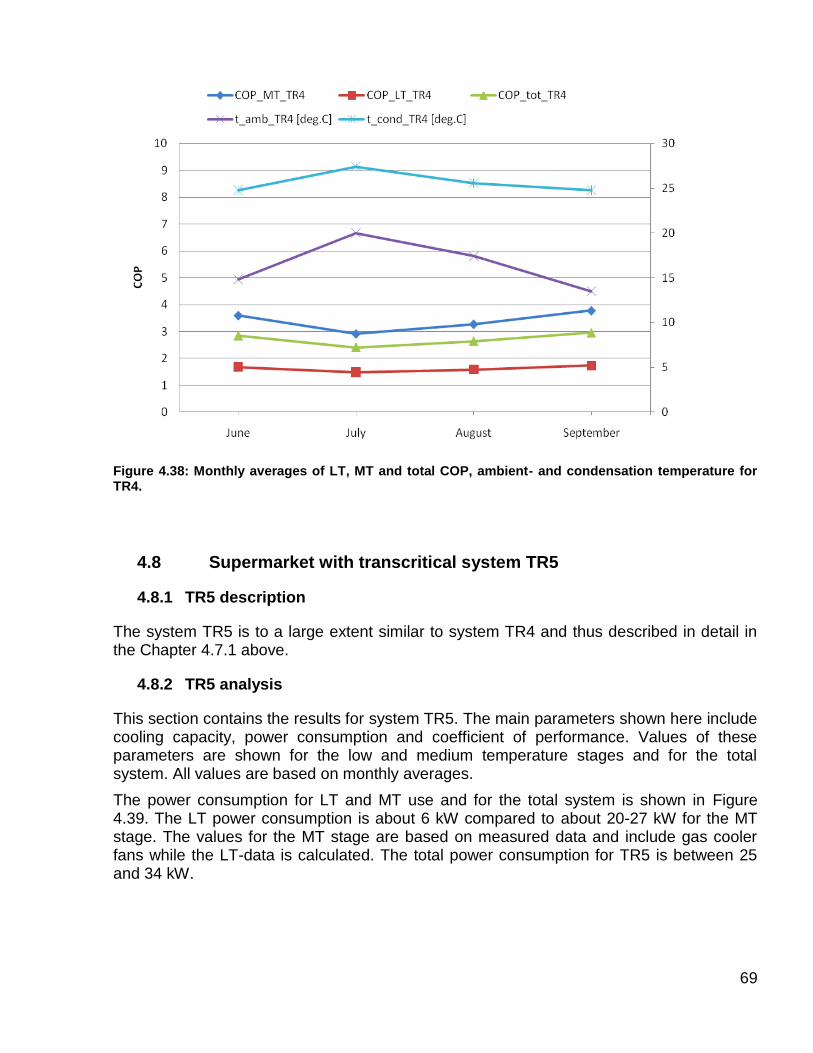
Figure 4.38: Monthly averages of LT, MT and total COP, ambient- and condensation temperature for TR4. .......................................................................................................... 69 Figure 4.39: Monthly averages of LT, MT and total power consumption, ambient- and condensation temperature for TR5. .................................................................................... 70 Figure 4.40: Monthly averages of LT, MT and total cooling capacity, ambient- and condensation temperature for TR5. .................................................................................... 71 Figure 4.41: Monthly averages of LT, MT and total COP, ambient- and condensation temperature for TR5. .......................................................................................................... 71

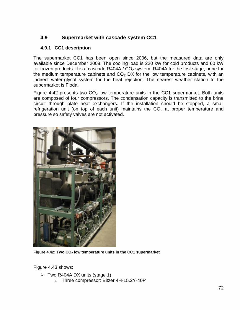
Figure 4.42: Two CO2 low temperature units in the CC1 supermarket ............................... 72

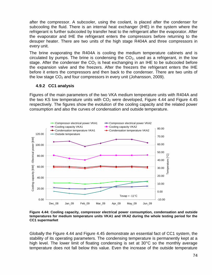
Figure 4.43: Schematic diagram of the cooling system in the supermarket CC1 ............... 73 Figure 4.44: Cooling capacity, compressor electrical power consumption, condensation and outside temperatures for medium temperature units VKA1 and VKA2 during the whole testing period for the CC1 supermarket .............................................................................. 74 Figure 4.45: Cooling capacity, compressor electrical power consumption, condensation and outside temperatures for low temperature units KS5 and KS6 during the whole testing period for the CC1 supermarket ......................................................................................... 75 Figure 4.46: COP for each units during the whole testing period for the CC1 supermarket. ........................................................................................................................................... 76 Figure 4.47: Freezer unit KS4 in system CC2 .................................................................... 77 Figure 4.48: Full system schematic for CC2 including all components and measurement points. ................................................................................................................................. 79

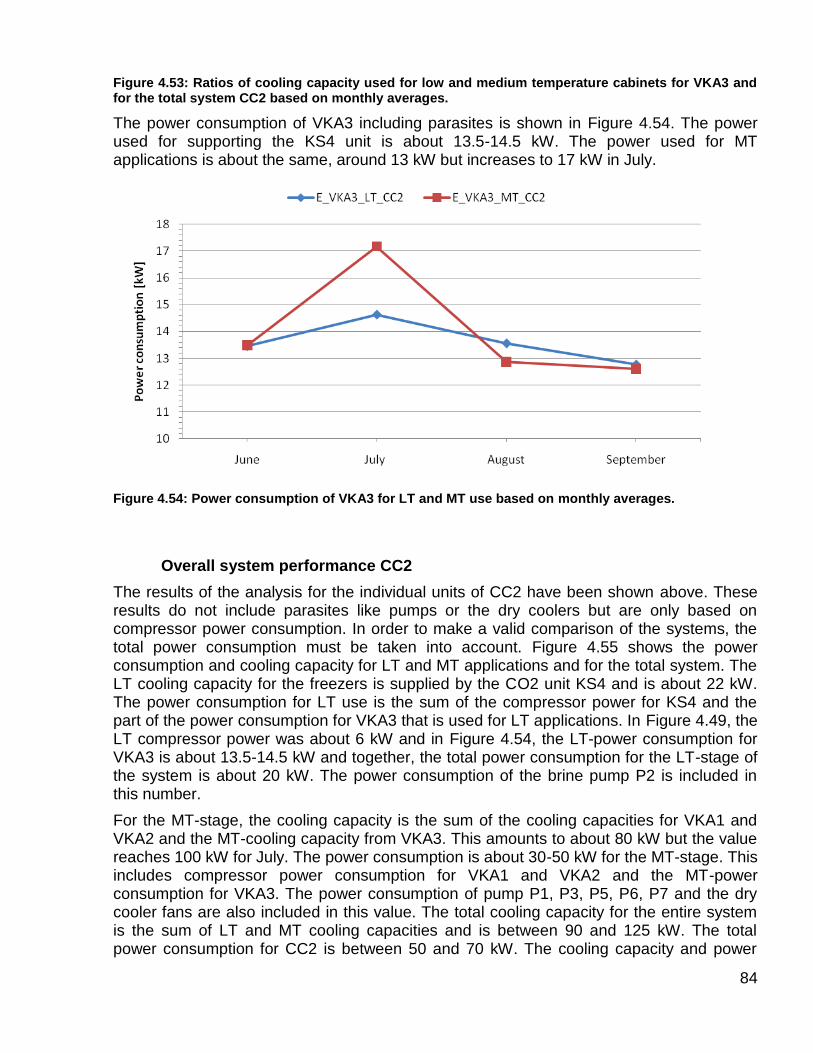
Figure 4.49: Monthly averages of outdoor temperature and compressor power consumption for the units of CC2. ........................................................................................................... 80 Figure 4.50: Monthly averages of outdoor temperature and cooling capacity for the different units of CC2. ....................................................................................................................... 81 Figure 4.51: Monthly averages of COP (excluding parasites) and outdoor temperature for the units of CC2. ................................................................................................................. 82 Figure 4.52: Ratios of cooling capacity that VKA1, VKA2 and VKA3 each supply to the medium temperature cabinets based on monthly averages. .............................................. 83 Figure 4.53: Ratios of cooling capacity used for low and medium temperature cabinets for VKA3 and for the total system CC2 based on monthly averages. ...................................... 84

Figure 4.54: Power consumption of VKA3 for LT and MT use based on monthly averages. ........................................................................................................................................... 84 Figure 4.55: Monthly averages of LT, MT and total cooling capacities and power consumption for CC2. ......................................................................................................... 85

Figure 4.56: LT, MT and total COP for system CC2 based on monthly averages. ............. 86 Figure 4.57: Monthly averages of brine supply- and return temperatures for MT cabinets in CC2. ................................................................................................................................... 86 Figure 4.58: Schematic diagram of the cooling system in the supermarket CC3 ............... 87 Figure 4.59: Refrigeration system CC3: IWMAC measured points at medium temperature level unit. ............................................................................................................................ 88

Figure 4.60: Refrigeration system CC3: IWMAC measured points at low temperature level unit. .................................................................................................................................... 89 Figure 4.61: The deviation between measured condensing temperature and predicted using linear regression method .......................................................................................... 90 Figure 4.62: Refrigeration system CC3 dry cooler unit energy usage correlation............... 91 Figure 4.63: Bitzer compressor mass flow estimation based on polinomial generation. ..... 91 Figure 4.64: Schematic diagram of the cooling system in the supermarket PC1................ 93

Figure 4.65: Refrigeration system PC3: IWMAC measured points (left) at medium (center) and low (right) temperature level units. .............................................................................. 94 Figure 5.1: Total COP with a load ratio of 3 in function of the condensing temperature for all the systems analysed ......................................................................................................... 97 Figure 5.2: Total COP* with a load ratio of 3 in function of the condensing temperature for the three systems analysed ................................................................................................ 98 Figure 5.3: COP* of the medium temperature parts for all systems versus their respective condensing temperatures ................................................................................................... 99

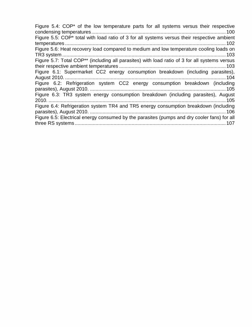
Figure 5.4: COP* of the low temperature parts for all systems versus their respective condensing temperatures ................................................................................................. 100 Figure 5.5: COP* total with load ratio of 3 for all systems versus their respective ambient temperatures .................................................................................................................... 102

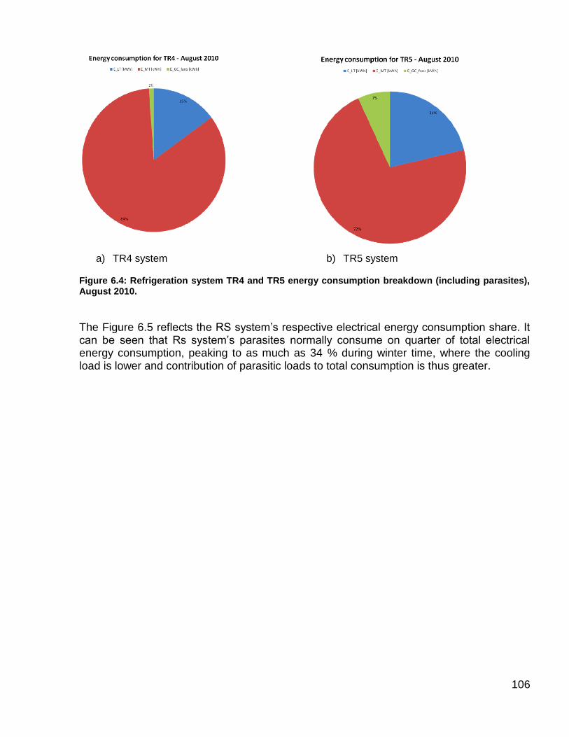
Figure 5.6: Heat recovery load compared to medium and low temperature cooling loads on TR3 system ...................................................................................................................... 103 Figure 5.7: Total COP** (including all parasites) with load ratio of 3 for all systems versus their respective ambient temperatures ............................................................................. 103 Figure 6.1: Supermarket CC2 energy consumption breakdown (including parasites), August 2010. .................................................................................................................... 104 Figure 6.2: Refrigeration system CC2 energy consumption breakdown (including parasites), August 2010. .................................................................................................. 105 Figure 6.3: TR3 system energy consumption breakdown (including parasites), August 2010. ................................................................................................................................ 105 Figure 6.4: Refrigeration system TR4 and TR5 energy consumption breakdown (including parasites), August 2010. .................................................................................................. 106

Figure 6.5: Electrical energy consumed by the parasites (pumps and dry cooler fans) for all three RS systems ............................................................................................................. 107

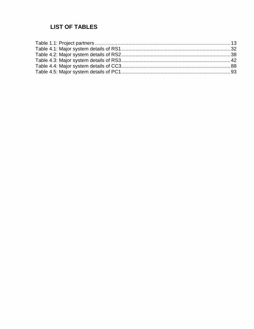
LIST OF TABLES

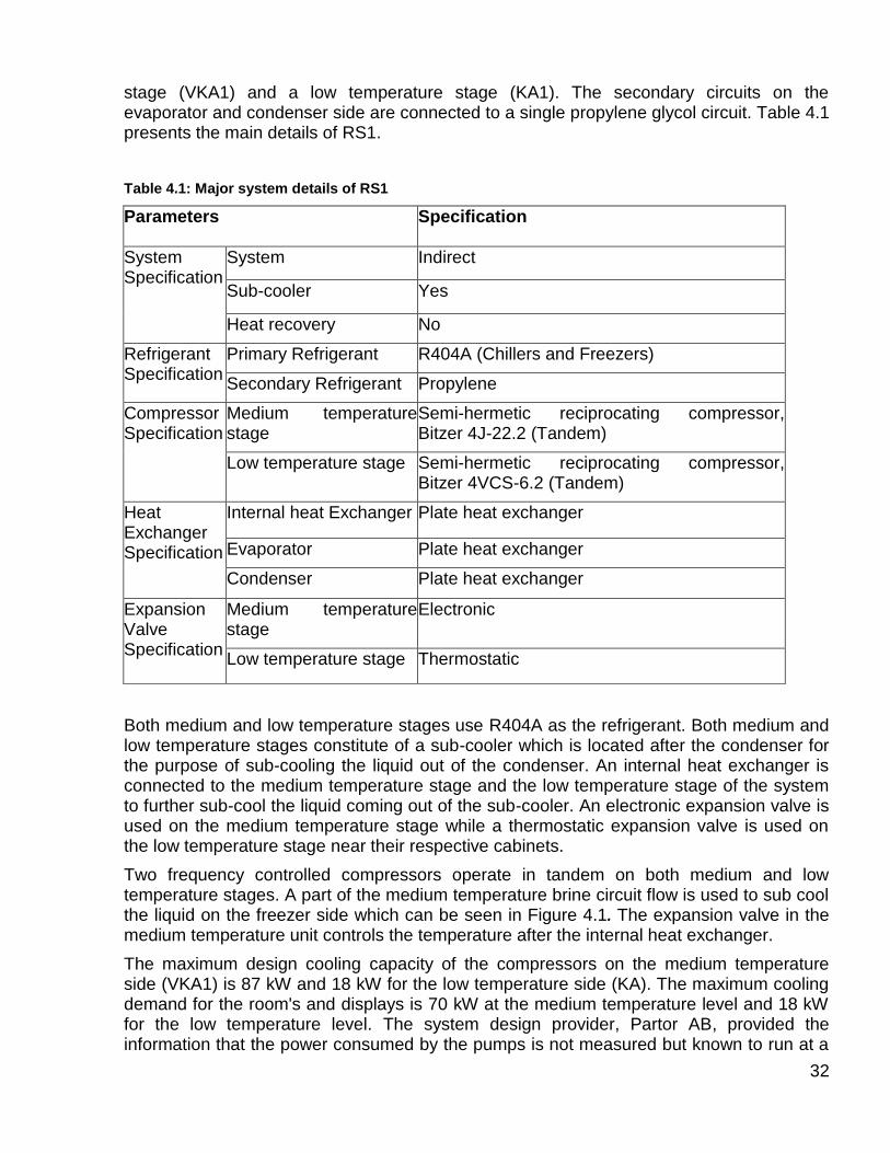
Table 1.1: Project partners ................................................................................................. 13 Table 4.1: Major system details of RS1 .............................................................................. 32 Table 4.2: Major system details of RS2 .............................................................................. 38 Table 4.3: Major system details of RS3 .............................................................................. 42 Table 4.4: Major system details of CC3 .............................................................................. 88

Table 4.5: Major system details of PC1 .............................................................................. 93

NOMENCLATURE

CC Cascade refrigeration system

22 COorCO Carbone dioxide

COP Coefficient of performance [-]

DX Direct expansion

E Electrical power [kW]

h Enthalpy [kJ/kg]

IHE Internal heat exchanger

HC Hydrocarbons

HFC Hydrofluorocarbons

HVAC Heating, Ventilating, and Air Conditioning

IHE Internal heat exchanger

KA Medium temperature unit or cabinet

KAFA Booster system with low and medium temperature

LT Low temperature

LR Load ratio

corrLR Load ratio correction, fixed value

m Mass flow [kg/s]

MT Medium temperature

NH3 or NH3 Ammonia

P Pressure [bar absolute]

PR Pressure ratio [-]

cQ Condensation capacity [kW]

oQ Cooling capacity [kW]

vq Volumetric refrigeration effect [kJ/m3]

RS Reference System

SC Subcritical refrigeration system

SH Superheat [K]

T Temperature [°C]

TR Transcritical refrigeration system

V Volume flow [m3/s]

Greek

Difference [-]

Density [kg/m3]

is Isentropic efficiency [-]

v Volumetric efficiency [-]

tot Total efficiency [-]

Specific volume [m3/kg]

Subscript

abs Absolute

amb Ambient

booster Booster system

brine Brine

cab Cabinet medium temperature

chiller Chiller

comp Compressor

cond Condenser

corr Corrected

el Electric

evap Evaporation

in Inlet

is Isentropique

freezer Freezer

gc Gas cooler

losses Heat losses

LR Load ratio

map Map or design conditions

new New or running conditions

out Outlet

cooleroil Oil cooler losses

V Volume

s Swept

pumps Pumps

sat Saturation

state State

tot Total

13

1. INTRODUCTION

The work, summarized in current report, has started as an investigation of different refrigeration systems solutions performance.

Usage of natural refrigerant has become the hot topic in recent times after the introduction of legislations to control manufacturing and usage of manmade refrigerants. Usage of natural refrigerants cannot become the solution to the environmental problems if the natural refrigerant based system solutions are not energy efficient. The performance and efficiency of the refrigeration system depends on various parameters such as demand, control strategies, climatic conditions etc. Only by evaluation of the installed system solutions this new technology can be facilitated.

The long-term refrigeration systems solutions performance evaluation results are summarized in this report.

1.1 Description of the project

Sveriges Energi- & Kylcentrum (SEK) which is a subsidiary company of Installatörernas Utbildingscentrum (IUC) in Katrineholm initialized this project work in order to analyse and evaluate the application of CO2-based technologies in supermarkets with a focus on energy efficiency and environmental issues. In many CO2 supermarket installations in Sweden analysis have not been carried out to study the performance of the systems. Previously investigations have been done on CO2 supermarket system solutions as a cooperation project between SEK and KTH which included computer simulation modelling and experimental work. The projects have suggested that CO2-based system solutions can be an efficient alternative to conventional solutions.

The project partner organisations and respective participants are presented in

Table 1.1.

Table 1.1: Project partners

Organisation Participant/s

Sveriges Energi- & Kylcentrum Jörgen Rogstam KTH - Energiteknik Björn Palm / Samer Sawalha

ICA Per-Erik Jansson Green and Cool Micael Antonsson

Partor AB Martin Johanson WICA Peter Rylander

Ahlsell Torbjörn Larsson Huurre Göran Sundin

AGA Christer Hens Tranter Ulf Vestergren Cupori David Sharp

Oppunda Svets Ken Johansson Energimyndigheten Conny Ryytty

14

1.2 Methodology and Objectives

The objectives of the project are to analyse, evaluate and compare the performance of a number of supermarkets: three of which are HFC-based refrigeration system solutions, five supermarkets which are CO2-based refrigeration system solutions, three supermarkets which combine CO2- and HFC-based refrigeration system solutions in the form of cascade refrigeration systems (3 supermarkets) and pump circulation system (1 supermarket).

Thus the report summarises previous analysis and evaluation results achieved by David Frelechox (Frelechox, 2009), Loius Tamilarasan (Tamilarasan, 2009), Sarah Johansson (Johansson, 2009) as well as provides new evaluation results made by Pavel Makhnatch, Johan Kullheim (Kullheim, 2011) and Yohann Caby (Caby, 2010).

All these HFC and CO2-based supermarket refrigeration systems are different in terms of varying load, climatic conditions, configurations and control. Although there are differences among these refrigeration systems a fair comparison will be established.

The method used in order to achieve the results described in this report includes:

Collecting information on the HFC- and CO2-based refrigeration systems installed in the supermarkets;

Creating data collection and calculation templates;

Measured data collection;

Data processing and calculation of necessary parameters, mainly COP's;

Comparing the supermarket refrigeration systems analysed;

Propose improvement possibilities for the supermarket refrigeration systems.

15

2. REFRIGERATION SOLUTIONS

In general, two temperature levels are required in supermarkets for chilled and frozen products. Product temperatures of around +3°C and –18°C are commonly maintained. In these applications, there are mainly three design options: indirect system, cascade DX system or transcritical DX system. It is also possible to advantage of different system and built mixed system.

2.1 Indirect systems

The main refrigeration circuit, of the conventional type with HFC or NH3, conveys heat from the main evaporator to the secondary fluid, which is pumped, obviously in liquid state, into the evaporators positioned inside the units to be refrigerated. The secondary fluid CO2 evaporates and removes heat from the units. The circulation ratio of the CO2 in the secondary circuit is generally between 1.5 and 3, and its highest operating temperature is at -10°C and lowest at -40°C. The following Figure 2.1 shows a schematic of the system and the cycle on the h-logP diagram.

a) Simplified indirect system layout b) Ph-diagram

Figure 2.1: Secondary fluid systems with phase change (Girotto, 2005).

Compared to traditional indirect systems, with propylene or ethylene glycol, the system in question requires lower flow rates and consequently smaller pipes and less pumping power and of course does not feature any change in temperature in the evaporators. The solution with forced circulation of CO2 offers major advantages in very extensive systems, with hundreds of metres between the units to be refrigerated and the central refrigeration unit, main advantages are (Girotto, 2005):

non-toxic fluid in circulation

16

no problem as regards the return of the oil regarding DX systems

low energy consumption for pumping regarding indirect brine systems

2.2 Cascade DX systems

At low temperatures (evaporation at temperature below -30°C) the cascade system is preferable. As can be seen on the Figure 2.2, two refrigeration units, each optimised for its own operating range, are thermally linked in series by means of an intermediate exchanger, which for one of the units represents the evaporator and for the other, the condenser.

For commercial refrigeration, for cost reasons, R404A or R507 are used in the high-temperature circuit, while NH3 is used for industrial refrigeration, this is especially suitable for this application because each NH3 and CO2 operates in its optimum temperature range. The risk related to the use of NH3 in premises where there could be people is thus eliminated, and this represents a big advantage.

For evaporation temperatures around -30°C, in applications where well water can be used as heat source, instead of using a cascade system with NH3, it could be possible to operate in single stage with the CO2 system, in the event of the size of the compressors available today for a supply pressure of up to 70 bar being big enough. In cold climates, air from outside could even be used for most of the year (Girotto, 2005).

a) Cascade DX system layout b) Ph-diagram

Figure 2.2: Direct expansion system in cascade (Girotto, 2005).

17

2.3 Transcritical DX systems

What separates trans-critical systems from other systems is the ability to reject heat at a state above the critical point. At pressures higher than the critical point, there is no saturated condition and temperature is independent of pressure. This means that both temperature and pressure have a separate influence on cooling capacity and COP. In the trans-critical region, COP is a function of the gas cooler outlet temperature and the discharge pressure. This means, that for each gas cooler outlet temperature, there is an optimum value of high stage discharge pressure (Likitthammanit, 2007). Since the refrigerant is a gas when above the critical point, the heat rejection process is referred to as “gas cooling” for trans-critical operation. Figure 2.3 shows a simplified schematic of a trans-critical CO2 system. The low and high stages are separated and both connected to a coolant loop for the heat rejection. The medium temperature unit has single-stage compression and the low temperature unit has two-stage compression with inter-cooling.

Figure 2.3: Simplified trans-critical CO2 system with two-stage compression and inter-cooling for the low temperature unit and single stage compression for the medium temperature unit (left) and Ph diagramm for one stage (right).

The ambient conditions affect the operation of this type of system. When the ambient temperature is high, the system mainly operates in a trans-critical mode, but for low ambient temperatures, the cycle is sub-critical. Because of the high pressure ratio and corresponding high compressor energy consumption that is required for trans-critical operation, trans-critical CO2 systems are best suited for cold climates. One of the main advantages with using CO2 as the only refrigerant in the cycle is that it eliminates the temperature differences that are present in the heat exchangers of indirect and cascade systems (Johansson, 2009).

18

3. MEASUREMENTS AND EVALUATION METHODS

The important parameters for the evaluation of cooling systems are mainly the cooling capacities and the COPs. For these capacities, the temperatures and pressures are needed to determine the enthalpies and then the mass flow rate is needed in order to determine the cooling capacities and different losses. Mass flow rate is not measured directly and it is normally evaluated from the compressor side. Then COPs are calculated using the cooling capacity and the measured or calculated electrical consumption. This chapter presents general approach to the measurements and the data evaluation in the supermarkets. More detailed description could be found in the previous studies reports.

3.1 Pressure and temperature.

The input data for the calculation of the refrigerant thermodynamics states are the measures of pressure and temperature. The temperature sensor types are generally PT100 or PT1000 and widely used in the refrigeration regulation. Pressure sensors give an absolute or relative pressure depending on their initial settings. The sensors used are generally from the manufacturer Danfoss and types are AKS or HSK according to their pressure range.

The sensors were mainly not installed especially for our study but are primarily used to operate the systems and are essential regulation elements. On the Figure 3.1 there is an example, which shows the measurement points distribution over the CO2 transcritical supermarket system. These points allow tracing the refrigeration cycle in the h-logP diagram and calculating the cooling capacity as well as various parameters which could influence this capacity, such as the internal and external superheat, the subcooling and the pressure ratio.

Two different systems have been used for the data acquisition:

IWMAC for TR1, TR2, TR3, CC2, CC3 and PC1 supermarket (Iwmac, 2009)

RDM with an interval of 15 minutes for CC1 supermarket (RDM, 2009)

Long Distance Service, LDS, for TR4 and TR5

ViSi+ software for RS1, RS2 and RS3 (see Figure 3.2)

19

Figure 3.1: Schematic of a CO2 Transcritical Supermarket with the pressure and temperature measurement points.

Figure 3.2: ViSi+ interface for referent system

20

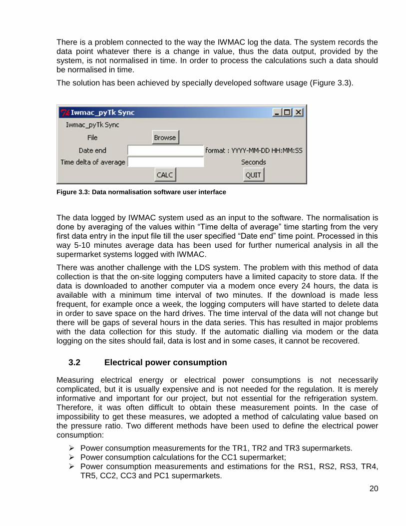
There is a problem connected to the way the IWMAC log the data. The system records the data point whatever there is a change in value, thus the data output, provided by the system, is not normalised in time. In order to process the calculations such a data should be normalised in time.

The solution has been achieved by specially developed software usage (Figure 3.3).

Figure 3.3: Data normalisation software user interface

The data logged by IWMAC system used as an input to the software. The normalisation is done by averaging of the values within “Time delta of average” time starting from the very first data entry in the input file till the user specified “Date end” time point. Processed in this way 5-10 minutes average data has been used for further numerical analysis in all the supermarket systems logged with IWMAC.

There was another challenge with the LDS system. The problem with this method of data collection is that the on-site logging computers have a limited capacity to store data. If the data is downloaded to another computer via a modem once every 24 hours, the data is available with a minimum time interval of two minutes. If the download is made less frequent, for example once a week, the logging computers will have started to delete data in order to save space on the hard drives. The time interval of the data will not change but there will be gaps of several hours in the data series. This has resulted in major problems with the data collection for this study. If the automatic dialling via modem or the data logging on the sites should fail, data is lost and in some cases, it cannot be recovered.

3.2 Electrical power consumption

Measuring electrical energy or electrical power consumptions is not necessarily complicated, but it is usually expensive and is not needed for the regulation. It is merely informative and important for our project, but not essential for the refrigeration system. Therefore, it was often difficult to obtain these measurement points. In the case of impossibility to get these measures, we adopted a method of calculating value based on the pressure ratio. Two different methods have been used to define the electrical power consumption:

Power consumption measurements for the TR1, TR2 and TR3 supermarkets. Power consumption calculations for the CC1 supermarket; Power consumption measurements and estimations for the RS1, RS2, RS3, TR4,

TR5, CC2, CC3 and PC1 supermarkets.

21

The first method is easy. A measuring device collects consumption values with the same definition that the measures of pressure and temperature, so 5 or 15 minutes. The Figure 3.4 the electrical consumption for one day of July for the freezer (FA) unit and the chiller (KA) unit. The collecting interval is 5 minutes for this device, thus about 300 measurement points per parameters each days. There is, of course, a normalisation procedure utilised for data logged by IWMAC system (as in is described in the Chapter 3.1 above).

Figure 3.4: Compressor electrical power measured for one day in July 2008 (01.07.08) in TR1 Supermarket.

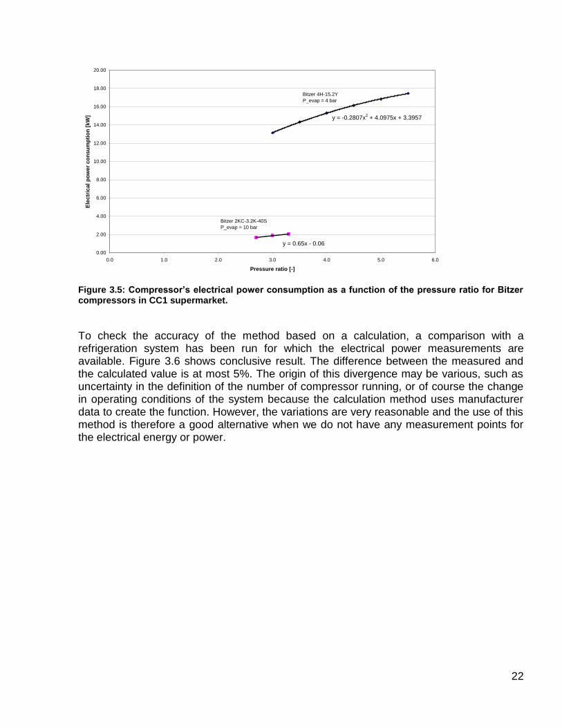
The second method uses a mathematic formula to calculate the power in function of the pressure ratio. Two formulas, used in CC1 refrigeration system, are shown on the Figure 3.5. The determination of this formula has been done with compressor manufacturer data (Bitzer, 2010). Obviously it is different for each type of compressor. The function is slightly different for each evaporation pressure, but this one is rather stable on our systems, so we decided to use the function for a given evaporation pressure. This gave satisfactory results.

22

Figure 3.5: Compressor’s electrical power consumption as a function of the pressure ratio for Bitzer compressors in CC1 supermarket.

To check the accuracy of the method based on a calculation, a comparison with a refrigeration system has been run for which the electrical power measurements are available. Figure 3.6 shows conclusive result. The difference between the measured and the calculated value is at most 5%. The origin of this divergence may be various, such as uncertainty in the definition of the number of compressor running, or of course the change in operating conditions of the system because the calculation method uses manufacturer data to create the function. However, the variations are very reasonable and the use of this method is therefore a good alternative when we do not have any measurement points for the electrical energy or power.

y = -0.2807x2 + 4.0975x + 3.3957

y = 0.65x - 0.06

0.00

2.00

4.00

6.00

8.00

10.00

12.00

14.00

16.00

18.00

20.00

0.0 1.0 2.0 3.0 4.0 5.0 6.0

Pressure ratio [-]

Ele

ctr

ical

po

we

r c

on

su

mp

tio

n [

kW

]

Bitzer 4H-15.2Y

P_evap = 4 bar

Bitzer 2KC-3.2K-40S

P_evap = 10 bar

23

Figure 3.6: Electrical power consumption, comparison with the two methods for a single stage CO2 system during the whole year 2008, KA1 unit in the TR1 Supermarket.

It should be noted that in all our calculations and simulations, we use the energy consumption of the compressors and for indirect systems we add also the energy consumption of the brine pumps. The power of the pumps was evaluated using the nominal power of the pumps, as no energy measurements have been available. Defrost heater, fans, lighting of the cabinets are not included.

3.3 Mass flow

The mass flow measurement is always a difficult process and is generally a key factor to obtain good results. None of the studied supermarkets had any mass flow measurement point. So method based on the pressure and temperature measures at the compressor inlet to get the specific volume was been used for the analysis. Official compressor manufacture data has been used to obtain the swept volume (Dorin, 2009) and (Bitzer, 2010), which is given as a fixed value in m3/h when the compressor is running under 50 Hz and the volumetric efficiency in function of the pressure ratio, as shown for some of the compressors on Figure 3.7. The swept volume multiplied by the volumetric efficiency could be seen as the volumetric flow through the compressor. In order to calculate the mass flow with Equation 3.1, the state (pressure and temperature) of the fluid at the compressor inlet were used to define the specific volume.

incomp

SVCO

v

Vm

_

2

Equation 3.1

0.00

5.00

10.00

15.00

20.00

25.00

30.00

Jan_

08

Feb_0

8

Mar

ch_0

8

Apr

il_08

May

_08

June

_08

July_0

8

Aug

_08

Sep

t_08

Oct_0

8

Nov

_08

Dec

_08

Ele

ctr

ical pow

er

consum

ption [kW

] -

Low

pre

ssure

[bar]

1.00

1.50

2.00

2.50

3.00

3.50

Pre

ssure

ratio [

-]

Compressor Power Measured Compressor Power Calculated Low pressure Pressure ratio

24

);(]/[

]/[

][

___

3

_

3

incompincompabsstateincomp

S

V

TPfkgmvolumespecificv

datacompressoronbasedsmvolumesweptV

fitteddatacompressoronbasedefficiencyvolumetric

Figure 3.7: Volumetric efficiency based on compressor data for three CO2 compressors

The following Figure 3.8 shows the variation of the CO2 mass flow during one day in July 2009 in the freezer system of the TR1 supermarket using the method based on the volumetric efficiency.

TCS373-D = -0.4079x2 - 6.5843x + 102.42

TCDH372= 0.0251x2 - 1.1706x + 93.424

SCS 362 SC = -0,1139x2 - 4,1854x + 95,12

0

10

20

30

40

50

60

70

80

90

100

0.00 2.00 4.00 6.00 8.00 10.00 12.00

Pressure ratio [-]

Vo

lum

etr

ic

eff

icie

ncy [

%]

TCS373-D

TCDH372 B-D

SCS 362 SC

25

Figure 3.8: Mass flow of CO2 in the freezer system FA1 during one day of July 2008 in the TR1 supermarket

As can be seen on the figure, the compressor inlet conditions are unstable mainly depending on the cooling capacity used in the cabinets and also the control of the internal superheat by the expansion valve, thus the compressor inlet temperature could vary quite a lot. The volume flow is quit constant because the pressure ratio is stable and the only things which affected are the number of compressor working. But the compressor inlet conditions of the fluid vary and affect the stability of the mass flow. Thus when only one compressor is working the mass flow of refrigerant could vary between 0.06 and 0.1 kg/s. In this case one or two compressors could be working. When the mass flow is above 0.1 kg/s then the second compressor has started working.

This method based on the volumetric efficiency has been chosen after several tests designed to apply the method that we consider the most reliable. Several researches have been held to find comparable methods in the literature. To assess the reliability of our method various comparisons have been made of which we present in the Figure 3.9 below.

0

0.05

0.1

0.15

0.2

0.25

30.06.2008

19:12

01.07.2008

00:00

01.07.2008

04:48

01.07.2008

09:36

01.07.2008

14:24

01.07.2008

19:12

02.07.2008

00:00

02.07.2008

04:48

CO

2 m

ass f

low

[kg

/s]

-25

-20

-15

-10

-5

0

5

10

15

20

Tem

pera

ture

[°C

] -

Pre

ssu

re [

bar]

CO2 mass flow Compressor inlet temperature Compressor inlet pressure

26

Figure 3.9: Mass flow of CO2 in a transcritical system for different mass flow measurement method

The first comparative method is the Dabiri‟s method based on an article proposed by Dabiri and Rice (Dabiri & Rice, 1982). Here, it is briefly summarized, firstly through Equation 3.2 which makes a ratio between design (map) conditions and actual (new) conditions:

11

map

new

map

new Fm

m

Equation 3.2

Where F is a chosen percentage of the theoretical mass flow rate increase (F = 0.75 is usually used) and where the densities are evaluated based on suction port conditions.

This method is difficult to apply because of the proposed correction factor is the result of experience with R22 and the experience is from 1982. Nonetheless, it has recently been used in laboratory test and gave satisfaction.

The second comparative method is based on the energy balance around the compressor according Equation 3.3. The compressor can be seen as a black box and the method is to do a simple energy balance.

cooleroillossescompel QQhmE

Equation 3.3

0.00

0.05

0.10

0.15

0.20

0.25

0.30

0.35

0.40

0.45

Jan_

08

Feb_0

8

Mar

_08

Apr

_08

May

_08

Jun_

08

Jul_08

Aug

_08

Sep

_08

Oct_0

8

Nov

_08

Dec

_08

Jan_

09

Feb_0

9

Mar

_09

Mass f

low

CO

2 [

kg/s

]

0.0

0.5

1.0

1.5

2.0

2.5

Pre

ssure

ratio

[-],

Eta

_to

t [-

]

mCO2 ηvol mCO2 Dabiri mCO2 15%Oil cooler Pressure Ratio Eta tot

27

The electrical consumption is measured and the enthalpy before or after the compressor is given from pressures and temperatures at the compressor inlet and outlet. Based on general experience and manufacturer information the heat losses are about 7% of electrical input and the oil cooler losses are about 15%. This last value does not seem to be a fix value as the oil cooler losses are affected from many parameters as the air or water inlet temperature and the pressure ratio of the compressor.

The Figure 3.9 shows differences between the three proposed methods. The first method based on compressor data has been finally chosen to use in the analysis because it seems the most reliable one. It is less dependent on external parameters than the others. The method of Dabiri is difficult to apply because of the use of a correction factor which is unreliable, particularly when we do not know the bases of this correction. Moreover, it seems to be very responsive to the pressure ratio and suffered large fluctuations. The evaluation of mass flow by the energy balance around the compressor uses fixed percentages of losses although the dissipated energy by the oil cooler fluctuates. Eta_tot is the total efficiency of the compressors including heat losses, oil coolers losses, isentropic losses, volumetric losses. Its value is around 0.6. The method we chose allows to calculate the heat dissipation in the oil cooler and to improve the technical knowledge of this item.

The Figure 3.10 below gives an overview of the effects of these various methods on our final objective, the COP calculation. Again, the method based on the volumetric efficiency, COPηvol, gives satisfactory results. It correlates very well with the COP resulting from the use of losses of 15% through the oil cooler, as well. In contrast, the method proposed by Dabiri and Rice seems doubtful. Indeed, it is hard to notice a real correlation with the pressure ratio while we know its importance on the efficiency of a system. The decrease of the pressure ratio in November 2008 does not really increase the COP which is unlikely.

Figure 3.10:COP of a CO2 transcritical system for different mass flow measurement method

0.0

1.0

2.0

3.0

4.0

5.0

6.0

Jan_

08

Feb_0

8

Mar

_08

Apr

_08

May

_08

Jun_

08

Jul_08

Aug

_08

Sep

_08

Oct_0

8

Nov

_08

Dec

_08

Jan_

09

Feb_0

9

Mar

_09

CO

P [

-],

PR

[-]

COP ηvol COP Dabiri COP 15%oil cooler Pressure Ratio

28

3.4 COP calculation

Eventually, the value that is important for the refrigeration systems performance analysis is the coefficient of performance of the system or COP. This value gives information about the efficiency of each system, thus provided, comparing them at identical operating conditions. The COP of a refrigeration system is calculated using the following Equation 3.4:

nconsumptiopowerElectrical

capacityCooling

E

QCOP

comp

o

inst

.

Equation 3.4

The equation above could be further modified in order to obtain a single value for the whole cooling system (as presented by the Equation 3.5):

)( ___

__

brinepumpchillercompfreezercomp

chillerofreezero

totEEE

QQCOP

Equation 3.5

A COP for the booster system must also be calculated. Since the high stage compressors and the booster compressors are located in different places in the system it is possible to calculate two mass flows. One mass flow is the total mass flow going through the high stage compressors and one mass flow is the mass flow maintaining the freezers. A mass balance can be applied to calculate the mass flow going through the medium temperature cabinets, see Equation 3.6

freezertotalchiller mmm

Equation 3.6

This mass flow and the pressure and temperature measurements allow calculating the power of each part of the system. Thus, the total COP of the booster system could be calculated in

Equation 3.7. Only the cooling capacity from the freezer side and the capacity from the medium temperature side which goes to the medium temperature cabinets is taken into account. The medium temperature power used for the condensation on the freezer side is eliminated.

chillercompfreezercomp

freezercchillerofreezero

boostertotEE

QQQCOP

__

___

_

Equation 3.7

For a cascade system, with the mass flow and the temperatures and pressure it is possible to calculate the cooling capacity of the R404A- and CO2-units ( Equation 3.8).

29

oo hmQ

Equation 3.8

where Δho is the enthalpy difference over the evaporator.

The condenser load of the CO2-unit can be calculated with Equation 3.9.

shaftfreezercompfreezerofreezerc EQQ ____

Equation 3.9

To decide the load of the medium temperature side cabinets

Equation 3.10 are used.

freezercchillerocabo QQQ ___

Equation 3.10

The electrical energy from the chiller which goes to the freezer can be calculated by Equation 3.11.

chillercomp

chillero

freezerc

freezerforchiller EQ

QE _

_

_

Equation 3.11

The COP for the freezers can be calculated by

Equation 3.12.

freezerpumpsfreezerforchillerfreezercomp

freezero

freezerEEE

QCOP

__

_

Equation 3.12

The COP for the chillers can be calculated by

Equation 3.13.

cabpumpsfreezerforchillerchillercomp

cabo

chillerEEE

QCOP

__

_

Equation 3.13

Where opumps QE %4 (Granryd, 2007)

To compare the concepts between each other, the load ratio has to be identical, i.e. the ratio of the cooling capacity between the chiller and the freezer is the same for each installation. An approximate value for European supermarket is 3, so 3 times more cooling

30

capacity for medium temperature cabinets than for low temperature cabinets. In order to correct our COP according to a fix load ratio (LRcorr), the Equation 3.14 has been developed (Frelechox, 2009). The abbreviation of load ratio is LR, thus COPtot_LR is the total COP of system with a defined load ratio LRcorr.

chillercomp

freezero

chillero

freezercomp

corr

corr

corrchillero

LRtot

EQ

QE

LR

LR

LRQ

COP

_

_

_

_

_

_1

1

Equation 3.14

Note that the COP is the instantaneous efficiency of the installation. It was calculated for each measurement interval (5, 10 or 15 minutes depending on the system analysed). Then averaging has been made to get a monthly value. It may slightly differ from the monthly COP which is a ratio of energy rather than power.

31

4. SYSTEMS’ DESCRIPTIONS AND PERFORMANCE ANALYSIS

This chapter summarises the work which has been done to evaluate the potential of refrigeration systems using carbon dioxide in supermarket refrigeration and their performance compared to traditional HFC-based systems. The results presented below based on previous measurements, evaluation and comparison of supermarket refrigeration systems held by Loius Tamilarasan, Sarah_Johansson, David Frelechox, Pavel Makhnatch, Johan Kullheim and Yohann Caby (Frelechox, 2009) (Tamilarasan, 2009) (Johansson, 2009) (Kullheim, 2011) (Caby, 2010). Thus more detailed information on respective systems‟ performance analysis is available in the above referred publications.

4.1 Supermarket refrigeration system RS1

4.1.1 RS1 description

Figure 4.1 shows the simplified circuit diagram of the reference systems.

Figure 4.1: Simplified circuit of the reference refrigeration systems

RS1 is open since the month of October 2008 and is located in the northern part of Sweden. The refrigeration system in this supermarket consists of a medium temperature

32

stage (VKA1) and a low temperature stage (KA1). The secondary circuits on the evaporator and condenser side are connected to a single propylene glycol circuit. Table 4.1 presents the main details of RS1.

Table 4.1: Major system details of RS1

Parameters Specification

System Specification

System Indirect

Sub-cooler Yes

Heat recovery No

Refrigerant Specification

Primary Refrigerant R404A (Chillers and Freezers)

Secondary Refrigerant Propylene

Compressor Specification

Medium temperature stage

Semi-hermetic reciprocating compressor, Bitzer 4J-22.2 (Tandem)

Low temperature stage Semi-hermetic reciprocating compressor, Bitzer 4VCS-6.2 (Tandem)

Heat Exchanger Specification

Internal heat Exchanger Plate heat exchanger

Evaporator Plate heat exchanger

Condenser Plate heat exchanger

Expansion Valve Specification


Electronic

Low temperature stage Thermostatic

Both medium and low temperature stages use R404A as the refrigerant. Both medium and low temperature stages constitute of a sub-cooler which is located after the condenser for the purpose of sub-cooling the liquid out of the condenser. An internal heat exchanger is connected to the medium temperature stage and the low temperature stage of the system to further sub-cool the liquid coming out of the sub-cooler. An electronic expansion valve is used on the medium temperature stage while a thermostatic expansion valve is used on the low temperature stage near their respective cabinets.

Two frequency controlled compressors operate in tandem on both medium and low temperature stages. A part of the medium temperature brine circuit flow is used to sub cool the liquid on the freezer side which can be seen in Figure 4.1. The expansion valve in the medium temperature unit controls the temperature after the internal heat exchanger.

The maximum design cooling capacity of the compressors on the medium temperature side (VKA1) is 87 kW and 18 kW for the low temperature side (KA). The maximum cooling demand for the room's and displays is 70 kW at the medium temperature level and 18 kW for the low temperature level. The system design provider, Partor AB, provided the information that the power consumed by the pumps is not measured but known to run at a

33

"constant" speed consuming roughly the same amount of energy throughout the year further the power consumed by the pump on the low temperature side is 1.5 kW and the power consumed by the coolant pump is 1.5 kW (Johannson, 2009).

Temperatures, pressures and compressors electric motor frequencies are measured since the time of installation for every 5 minutes interval and logged in the data base system SAIA- ViSi+ (Sicatron, 2009). In total the system performance has been studied since October 2008 until June 2010. However, due to measurement system failure there is no data measured for February 2010. Further analysis charts are plotted for the period covering last full year of observation, thus from Jun 209 till June 2010.

4.1.2 RS1 analysis

One of the most important parameters which should be considered while studying the performance characteristics of the system is the cooling capacity. The cooling capacity for the system RS1 is presented and analysed for a period of total 12 months: from June 2008 till January 2010 and from March 2010 till June 2010.

The Figure 4.2 shows the mains parameters of RS1 for the medium temperature unit during the observation period. This plot shows the cooling capacity, the electrical power consumption, the evaporating temperature, and the outdoor temperature. The cooling capacity depends of the electrical consumption and is influence by the outdoor temperature.

Figure 4.2: System RS1: main parameters for the medium temperature side during the observation period

-20

-15

-10

-5

0

5

10

15

20

0

10

20

30

40

50

60

70

80

Tem

pe

ratu

re [

°C]

Co

olin

g ca

pac

ity

[kW

] -

Ele

ctri

cal c

on

sum

pti

on

[k

W]

Cooling capacity_chiller Electrical consumption_chiller

Outdoor temeperature Evaporating temperature_chiller

34

The Figure 4.3 shows the cooling capacity, the electrical consumption, the evaporating temperature, and the outdoor temperature during one year. The evaporating temperature is almost constant during the year it means -8°C for the chillers and -29°C for the freezers.

Figure 4.3: System RS1: Main parameters for the low temperature side during the observation period

The cooling capacity on the medium temperature side has more fluctuation than the low temperature side. The reason is the low temperature cabinets have a glass doors which decrease the heat exchange with the ambient. The fluctuation of the cooling capacity for the medium temperature side is around 25kW (let 28% of the maximum design cooling capacity) although for the low medium side it is around 3kW (let 17% of the maximum design cooling capacity).

A peak of electrical consumption appears during the summer period in order to provide enough cooling power. The electrical consumption decreases during the winter. The ambient temperature has an influence on the condensing temperature and so has an influence on the compressor power consumption.

So the condensing temperature has en influence on the performance of the system. The condensing temperature for the medium temperature side is around 22°C while for the low temperature side the condensing temperature is around 16°C. Indeed, the Figure 4.4 shows, the differential of temperature between the condensing temperature and the outdoor temperature is one time and half important on the chiller that on the freezers. The condensing temperature for the chiller is a bit too high but it is a design default. The one way valve which located on the compressor discharge is sized very small hence causing a higher pressure drop in the compressor discharge line which in turn leads to a higher discharge pressure than necessary.

-40

-30

-20

-10

0

10

20

0

2

4

6

8

10

12

14

Tem

pe

ratu

re [

°C]

Co

olin

g ca

pac

ity

[kW

] -E

lect

rica

l co

nsu

mp

tio

n

[kW

]

Cooling capacity_freezer Electrical consumption_freezer

Evaporating temeperature_freezer Outdoor temperature

35

Figure 4.4: System RS1: condensing temperature for the medium and low temperature side, outdoor temperature, and the differential of temperature between the condensing temperature and the outdoor temperature.

The Figure 4.5 shows the COP trend during the year. It appears clearly the COP decrease when the outdoor temperature increases, which increase the condensing temperature of the system. The high condensing temperature is the consequence of the low COP.

Figure 4.5: System RS1: Coefficient of performance for the chiller and the freezer

-20

-10

0

10

20

30

40

0

5

10

15

20

25

30

35

40

45

50

Tem

pe

ratu

re [

°C]

dT

[K]

freezer dT chiller dT

Condensing temperature_chiler Condensing temperature_freezer

Outdoor temperature

-20

-15

-10

-5

0

5

10

15

20

0

1

2

3

4

5

6

Tem

pe

ratu

re [

°C]

CO

P [

-]

COP_chiller COP_freezer Outdoor temperature

36



This supermarket was opened in the month of October 2008. In this system there are two medium temperature and two low temperature level circuits (VKA1&2 and KA1&2). R407C is the refrigerant used on the medium temperature stage while R404A is used on the low temperature stage. The secondary circuits on the evaporator and condenser sides are connected to the ethylene glycol circuit.

The liquid after the condenser is sub-cooled on both medium and low temperature levels with the use of a sub-cooler. An internal heat exchanger is also installed on the medium temperature and low temperature levels to further sub-cool the liquid coming out of the sub cooler and also to superheat the suction gas into the compressor. In the case of the low temperature stage the internal heat exchanger is placed in the cabinet and in the case of medium temperature stage the internal heat exchanger is present after the evaporator and before the compressor inlet similar to that of RS1.

Figure 4.6 and Figure 4.7 presents the medium temperature and low temperature stages in the supermarket refrigeration system RS2. It is clear from both figures that two compressors using frequency control work in tandem on the medium temperature side while single frequency controlled compressor is operated on the low temperature stage.

Figure 4.6: Medium temperature stage (VKA1) of the refrigeration system RS2

37

Figure 4.7: Low temperature stage (KA1) of the refrigeration system RS2

Temperatures, pressures and compressor electric motor frequencies are measured at various points of the system and logged in the data base since the time the system was installed. System RS2 constitutes of two frequency controlled compressors working in tandem on the medium temperature stages (VKA1&2) while a single frequency controlled compressor is utilized on the low temperature stages (KA1&2).

From Figure 4.1 we are also able to see that a part of the compressor work on the medium temperature side is utilized to sub-cool the low temperature side. A pump is used to pump the refrigerant from the evaporator to the cabinet and a part of it to the sub-cooler on the low temperature side.

Partor AB outlines that the pumps work at a constant speed consuming about the same power throughout the period the system works (Johannson, 2009). The power consumed by the pumps is not measured and is assumed to work constantly in the calculations. The power consumed by the pump on the brine side is 3kW and the coolant side is 3kW.

Table 4.2 presents the major system details of the refrigeration system RS2.

38




System Indirect

Sub-cooler Yes

Heat recovery No


Primary Refrigerant R404A (Freezers), R407C (Chillers)

Secondary Refrigerant Ethylene glycol



Semi-hermetic reciprocating compressor, Bitzer 4J-22.2 (Tandem)

Low temperature stage Semi-hermetic reciprocating compressor, Bitzer 4J13.2 (single)







Electronic


4.2.2 RS2 analysis

Reference system number 2 is located in Stockholm and the analysis period extends for up to 20 months from November 2008 to June 2010, 13 latest of which are presented here in further analysis. RS2 use two different refrigerants: refrigerant R407C is used in the medium temperature level while refrigerant R404A is used in the low temperature level.

The Figure 4.8 shows the monthly average of the condensing temperature for each unit (low and medium temperature unit) with the outdoor temperature during the observation period. It appears the condensing temperature is maintained to a same value for low and medium temperature units. However the unit VKA1 has always the highest condensing temperature.

39

Figure 4.8: System RS2: condensing temperature of each units and outdoor temperature during the observation period.

The Figure 4.9 shows the cooling capacity and the electrical power consumption of RS2. The lowest cooling capacity appears during the winter when the outdoor temperature is the lowest. However the variation of cooling capacity is higher for the medium temperature units than the low temperature units. The reason is the same as for RS1: the cabinets of the low temperature units are protected by a glass door which decreases the exchange with the ambient. On the contrary the highest cooling capacity appears during the summer period when the outdoor temperature is the highest.

The electrical power consumption follows the same trend like the cooling capacity but with less variation. The electrical consumption increases in summer and decrease in winter.

-10

-5

0

5

10

15

20

25

0

5

10

15

20

25

30

35

Ou

tdo

or

tem

pe

ratu

re [

°C]

Co

nd

en

sin

g te

mp

era

ture

[°C

]

Condensing temperature VKA1 Condensing temperature VKA2

Condensing temperature KA1 Condensing temperature KA2

Outdoor temperature

40

Figure 4.9: System RS2: cooling capacity and electrical consumption for low and medium temperature units during the observation period.

The Figure 4.10 shows the subcooling capacity during the year. The evaporating temperature is maintained at a rather constant value of -8°C for the medium temperature side and -32°C for the low temperature side. It can be noticed that the subcooling capacity is the highest during the summer and the lowest during the winter. The trend of the subcoolng capacity follows the trend of the outdoor temperature.

Figure 4.10: System RS2: average of the subcooling for both freezers units, evaporating temperature for the low and the medium temperature side, and the outdoor temperature during the observation period

-10

-5

0

5

10

15

20

25

0102030405060708090

100

Tem

pe

ratu

re [

°C]

Co

olin

g ca

pac

ity

[kW

] -

Ele

ctri

cal

con

sum

pti

on

[kW

]

Cooling capacity chiller Electrical consumption chiller

Cooling capacity freezer Electrical consumption freezer

Outdoor temperature

-40

-30

-20

-10

0

10

20

30

0

1

2

3

4

5

6

7

Tem

pe

ratu

re [

°C]

Sub

coo

ling

cap

acit

y [k

W]

KA_subcooling capacity Evaporating temeprature chiller

Evaporating temperature freezer Outdoor temperature

41

The Figure 4.11 shows the evolution of the COPs during the year for RS2. The highest COP is during the winter; it is logical because the demand is the lowest and the condensing temperature is reduced with the low outdoor temperature. On the contrary the COP is the lowest during the summer when the cooling demand is the higher and the outdoor temperature doesn‟t permit a low condensing temperature. So the maximum COP for the chiller is 4.7 and for the freezer is 3.

Figure 4.11: System RS2: COP for the chillers units and the freezers units during the observation period.

-10

-5

0

5

10

15

20

25

0

0,5

1

1,5

2

2,5

3

3,5

4

4,5

5

Tem

pe

ratu

re [

°C]

CO

P [

-]

COP chiller COP freezer Outdoor temperature

42



This supermarket is open since March 2008. The system constitutes of two medium temperature stages (VKA1&2) and two low temperature stages (KA1&2). There is a mix of refrigerant usage in the medium temperature stage R404A is utilized on one of the medium temperature stages (VKA1) and R407C is utilized on the other medium temperature stage (VKA2). Both the temperature stages (KA1&2) utilize R404A as the refrigerant. Heat is recovered from the system (VKA5) and an air conditioner (VKA3) is also utilized during the summer period. Frequency controlled compressors work in tandem on both medium and low temperature levels.

Both medium and low temperature stages constitute of a sub-cooler each, used to sub-cool the liquid coming out of the condenser. An internal heat exchanger is present on the medium temperature stage to further sub-cool the liquid coming out of the sub-cooler. Compressor power on the medium temperature stage is utilized to sub-cool the freezers similar to that of RS 1 and 2. Temperatures, pressures and electric motor frequencies are measured and logged in the data base system (SAIA-ViSi+) (Sicatron, 2009). Measured data's are available since May 2009. Partor AB (Johannson, 2009) outlines that the pumps are assumed to work at a constant speed consuming the same power throughout the period the system works further the power consumed by the pumps is not measured and hence calculated by using the information given that the power consumed by the pump on the cold glycol is 6 kW and the warm glycol is 6 kW.




System Indirect

Sub-cooler Yes

Heat recovery Heat pump


Primary Refrigerant R404A (Freezers), R407C (Chillers) R404A(Chillers)

Secondary Refrigerant Propylene glycol


Medium temperature stage Semi-hermetic reciprocating compressor, Bitzer 6F-50.2 (Tandem)

Low temperature stage Semi-hermetic reciprocating compressor, Bitzer 4H-15.2 (Tandem)






Medium temperature stage Electronic


43

4.3.2 RS3 analysis

For RS3, the refrigerant R404A is used for the low temperature side and for one of the medium temperature unit (VKA1). The refrigerant R407C is used for the medium temperature unit VKA2.

The Figure 4.12 shows the cooling capacity and the electrical consumption for the low and the medium temperature units. The same observation can be applied on the cooling capacity and the electrical consumption; it means a higher cooling capacity during the summer period than during the winter period. The cooling capacity variation is less important on the low temperature side because the cabinets have a glass door which decreases the heat exchange with the ambient.

Figure 4.12: System RS3: cooling capacity and electrical consumption for the medium and the low temperature units.

The Figure 4.13 shows the subcooling capacity of the freezers units. The evaporating temperature is almost constant for the medium and the low temperature side. The evaporating temperature for the medium temperature units is -7. The evaporating temperature for the low temperature unit is -31°C.

The subcooling capacity decreases for the winter period when the outdoor temperature is low and so when the condensing temperature decreases too.

-10

-5

0

5

10

15

20

0

10

20

30

40

50

60

70

80

90

100

01-08-2009 01-09-2009 01-10-2009 01-11-2009 01-12-2009

Tem

pe

ratu

re [

°C]

Co

olin

g ca

pac

ity

[kW

] -

Ele

ctri

cal c

on

sum

pti

on

[k

W]

Cooling capacity chiller Electrical consumption chiller

Cooling capacity freezer Electrical consumption freezer

Outdoor temperature

44

Figure 4.13: System RS3: subcooling capacity and evaporating temperature of chillers and freezers during the observation period.

4.4 Supermarket with transcritical system TR1

4.4.1 TR1 description

The TR1 supermarket has been open since autumn 2007. The maximal cabinet design cooling load is 230 kW for cold products and 60 kW for frozen products. There are four separated transcritical units, two for the medium temperature cabinets and two for the low temperature, with an indirect water-glycol system for the heat rejection. The nearest weather station to the supermarket is Storön.

Figure 4.14 represents a refrigeration unit installed in the TR1 supermarket; three compressors are visible at the bottom of this unit. They produce the cooling capacity for the medium temperature. The 4th compressor is barely visible behind the electrical panel. On each compressor the oil cooler can be distinguished, oil heat is transferred to the coolant.

-40

-30

-20

-10

0

10

20

0

0,5

1

1,5

2

2,5

3

3,5

4

4,5

01-08-2009 01-09-2009 01-10-2009 01-11-2009 01-12-2009

Tem

pe

ratu

re [

°C]

Sub

coo

ling

cap

acit

y [k

W]

Subcooling capacity Evaporating temperature chiller

Evaporating temperature freezer Outdoor temperature

45

Figure 4.14: Refrigiration unit in TR1 Supermarket

Figure 4.15 shows:

Two Coolers o Transcritical CO2, single-stage / Compressor four Dorin TCS 373-D o Oil cooler o Heat recovery o Coolant

Two Freezers o Transcritical CO2, two-stages with intercooler / Compressor:

two Dorin TCDH 372 B-D

o Oil cooler o Heat recovery o Coolant

46

Figure 4.15: Schematic diagram of the TR1 system

The system is a parallel solution where there are two separate carbon dioxide circuits, one for the medium temperature side (KA1/KA2) and one for the cold temperature side (FA1/FA2). A benefit from using a parallel solution is that if one of the cycles fail, the other cycle can unaffectedly continue to work (Sawalha, 2008).

The cold temperature side, seen to the right in Figure 4.15, has a two-stage compression with an intercooler in between. This is arranged to achieve cold temperatures but still keep low pressure ratios in the compressors. This will lower the inlet temperature to the second compressor, decrease the discharge pressure after the second stage and decrease the losses, thereby increase the efficiency of the system. The carbon dioxide is condensed in the condenser and expanded in the expansion valve before entering the evaporator (freezers). The expansion valves are placed out in the supermarkets close to the evaporators. The reason is to minimize the losses in the system by transporting the refrigerant with high pressure. After the freezer the refrigerant return to the machinery room and enters a liquid separator before the compressors. This is done to make sure that no liquid is going in to the compressors. There are two units for the cold temperature side (FA1 and FA2). Each unit has two two-stage compressors.

The medium temperature side has a one-stage compressor since it doesn‟t need to operate with as high pressure ratio as the cold temperature side to maintain the chillers. After the condenser the refrigerant is expanded in the expansion valve where the pressure is reduced, before entering the evaporator (chillers). For the same reasons as in the FA-units, the expansion valves are placed in the Supermarket area close to the cabinets. There are two units for the medium temperature side (KA1 and KA2). There are four one-stage compressors in every unit.

The refrigerant in both cycles is gas cooled by brine circulating between the main condenser and the two CO2-cycles. The cold brine is used for the oil coolers and the condensers/gas coolers in both circuits and for the intercooler in the cold temperature side

47

see Figure 4.15. The brine condenser is placed on the roof and is using the outside air temperature to cool down the brine. There is an additional heat exchanger in the brine circuit, placed before the condenser, for maintaining a heat pump that is supplying the supermarket with air conditioning and heating (Johannson, 2009).

4.4.2 TR1 analysis

The Figure 4.20 shows the cooling capacity for the medium and low temperature units KA1 and FA1. A peak of consumption appears during the summer. This increase is particularly visible on the medium temperature unit as freezers, most of which are fitted with glass doors, are less responsive to ambient conditions.

Figure 4.16: Cooling capacity of one medium temperature unit (KA1) and one low temperature unit (FA1) during the years 2008 – 2009

The plot on Figure 4.16 is divided in curves for 2008 and 2009 because the system seems to have different control schemes during these periods. Since the end of 2008 the limit of the floating condensation was lowered. The elevated consumption during January and February 2008 on KA1 is linked to the commissioning of the cooling system. The installation was still in a settings stage. From 2008 to 2009 the load falls, while external conditions are almost identical and that the layout of the store has not changed. To our knowledge, no changes have been made on cabinets, the load should not vary. However, several external parameters may explain this decrease as decrease in a customer‟s numbers or an adjustment of the regulation on the HVAC system.

Some improvements on the system after the summer 2008 can also play a role in this development. The setting on the condensers‟ coolant temperature was lowered which led to a COP improvement and thus reduced the compressors‟ power consumption. This trend

0.00

10.00

20.00

30.00

40.00

50.00

60.00

70.00

Jan Feb Mar Apr May Jun Jul Aug Sep Oct Nov Dec

Co

olin

g c

ap

acity [

kW

]

-20.00

-15.00

-10.00

-5.00

0.00

5.00

10.00

15.00

20.00

25.00

30.00

Te

mp

era

ture

[°C

]

KA1 cooling capacity 2008 KA1 cooling capacity 2009 FA1 cooling capacity 2008

FA1 cooling capacity 2009 Outdoor temperature 2008 Outdoor temperature 2009

48

is clearly visible on Figure 4.21 below. The evaporation temperature has been rather constant all the way around -10°C for the medium temperature units and -35°C for the low temperature units.

Figure 4.17: Compressors electrical power consumption for one medium temperature unit (KA1) and one low temperature unit (FA1) during the years 2008 - 2009

The modification of the coolant temperature is particularly important. Its effect is clear on the consumption curve of FA1. Just after the change during August 2008, the power consumption decreases. To highlight the impact of coolant temperature on the COP, we present the Figure 4.42.

The data based on the field measurements show a clear correlation between the coolant temperature at the entrance of the condenser / gas cooler and the performance of the system. The impact on the COP of decreasing the coolant temperature is more important on medium temperature unit. This is evidently because of its lower pressure ratio.

0.00

5.00

10.00

15.00

20.00

25.00

Jan Feb Mar Apr May Jun Jul Aug Sep Oct Nov Dec

Ele

ctr

ica

l p

ow

er

[kW

]

0.00

5.00

10.00

15.00

20.00

25.00

30.00

35.00

40.00

Te

mp

era

ture

[°C

]

KA1 comp electrical consumption 2008 KA1 comp electrical consumption 2009

FA1 comp electrical consumption 2008 FA1 comp electrical consumption 2009

Coolant temperature 2008 Coolant temperature 2009

49

Figure 4.18: COP function of coolant temperature for medium temperature units and low temperature units, measures for TR1 supermarket during 2008.

Finally the Figure 4.43 shows the COP of each unit for the whole test period. The low temperature units FA 1 and 2 show small changes in function of the ambient conditions and also following the modification of the coolant temperature. In contrast, the medium temperature COP of the KA 1 and 2 units can vary from 2.8 to 4.5. This is the result of the use of the floating condensation which considerably increases the COP during the winter. From winter 2008 to winter 2009, the COP was improved of about 25 % following the lowering of the coolant temperature which was reduced from 12 to 7 K.

Figure 4.19: COP for each units during the whole testing period for the TR1 supermarket.

y = 0.0058x2 - 0.2932x + 6.3315

y = 0.0024x2 - 0.0957x + 2.2924

0.00

0.50

1.00

1.50

2.00

2.50

3.00

3.50

4.00

4.50

5.00

0.00 2.00 4.00 6.00 8.00 10.00 12.00 14.00 16.00 18.00 20.00

Coolant temperature [°C]

CO

P

COP_chiller_KA1 COP_chiller_KA2

COP_freezer_FA1 COP_freezer_FA2

Polynomial (COP_chiller_KA1) Polynomial (COP_freezer_FA2)

0.00

0.50

1.00

1.50

2.00

2.50

3.00

3.50

4.00

4.50

5.00

Jan_

08

Feb_0

8

Mar

_08

Apr

_08

May

_08

Jun_

08

Jul_08

Aug

_08

Sep

_08

Oct_0

8

Nov

_08

Dec

_08

Jan_

09

Feb_0

9

Mar

_09

Apr

_09

May

_09

Jun_

09

CO

P

COP KA1 COP KA2 COP FA1 COP FA2

50



The supermarket TR2 has been open since august 2008. The maximal cabinet design cooling load is 200 kW for cold products and 50 kW for frozen products. There are three separated transcritical units, two booster types for the medium temperature cabinets and the low temperature cabinets with a load ratio of about 2, and one standard-type for the rest of the medium temperature cabinets, with a direct system for the heat rejection. The nearest weather station to the supermarket is Gothenburg.

Figure 4.20 represents a booster unit installed in the TR2 supermarket. Three compressors are visible at the bottom of this unit. They produce the cooling capacity for the medium temperature. The two compressors for the low temperature are behind the electrical panel. On each compressor an air cooled oil coolers can be distinguished. On top of the large tanks, there are three valves to avoid overpressure in the system. The 3 tanks are used as receiver and oil separator.

Figure 4.20: Booster unit in TR2 Supermarket

Figure 4.21 shows:

Two Boosters o Transcritical CO2, two-stage intercooling booster o Compressor: two Dorin SCS 362 (low temperature level), three Dorin TCS

373 (high temperature level) o Oil cooler

51

o Heat recovery o Subcooling from ground heat sink o Gas cooler on the roof

Single Standard o Transcritical CO2, single-stage / four Dorin TCS 373 o Oil cooler o Heat recovery o Subcooling from ground heat sink o Gas cooler on the roof

Figure 4.21: Schematic diagram of the TR2 system

In this supermarket there are one circuit for the medium temperature side (KA3) and one circuit for a combined medium and cold temperature side (KAFA1/KAFA2). There are two units for the combined side (KAFA1 and KAFA2) and one unit for only medium temperature cabinets (KA3).

The KA3 cycle can be seen to the right in Figure 4.21 and is similar to the KA-unit in trans-critical system 1. After the evaporator (chillers) the refrigerant enters the one-stage compressor. An extra heat exchanger is placed after the compressor to recover heat to floor and space heating of the supermarket. The refrigerant is after that gas cooled/condensed in the gas cooler. The gas cooler is placed on the roof and uses the outside air temperature to cool down the refrigerant. Before the refrigerant reaches the expansion valve an extra heat exchanger is placed to further cool down the refrigerant and

52

gain some additional heat recovery. This heat exchanger uses a ground heat source for heat exchange with the carbon dioxide.

The combined circuit (KAFA1/KAFA2) side can be seen to the left in Figure 4.21 and it serves both medium temperature cabinets and freezers. The gas cooler is placed on the roof and uses the outside air to cool down the refrigerant. After the gas cooler/condenser the CO2 runs through an additional heat exchanger for heat recovery, which also uses the same ground heat source as in KA3. The ground heat source is used for heating the supermarket. The mass flow of the refrigerant is separated before it reaches the expansion valves and cabinets/freezers. After the freezers two compressors called “booster compressors” are located. They increase the pressure of CO2 to the same pressure as the CO2 has during the evaporation in the medium temperature cabinets. The mass flows from the medium temperature cabinets and from the freezers are mixed in the liquid separator before the high stage compressors. The high stage compressors raise the pressure of the CO2 to condensing pressure. The refrigerant runs through an additional heat exchanger, for floor and space heating as in the case of KA3-unit, before it is gas cooled/condensed in the gas cooler (Johansson, 2009).

4.5.2 TR2 analysis

A figure per unit has been achieved, KAFA 1 and 2 are booster units and KA3 is a medium temperature unit. These figures show the evolution of the cooling power and the related power consumption, the curves of condensing and outdoor temperature, as well as the effect of subcooling produced by the borehole. This effect is expressed by its ΔT in Kelvin. Note that the borehole is connected to the heat pump as well and used as heat source to heat the building during the winter.

Figure 4.22: Different parameters plots for the KAFA1 unit during the whole period of study in the TR2 supermarket

0.00

10.00

20.00

30.00

40.00

50.00

60.00

70.00

Sept_

08

Oct_0

8

Nov

_08

Dec

_08

Jan_

09

Feb_0

9

Mar

ch_0

9

April_

09

May

_09

June

_09

Coolin

g c

apacity [

kW

] -

Ele

ctr

ical pow

er

[kW

]

0.00

5.00

10.00

15.00

20.00

25.00

30.00

Tem

pera

ture

[°C

] -

dT

[K

]

Cooling capacity Compressor electrical consumption

Condensation temperature dT subcooling borehole

Outside temperature

Tevap = -10°C / -35°C

53

Figure 4.22 shows, as expected a cooling capacity drop during the winter. In contrast the power consumption does not follow the same trend, although logically it should take advantage of low winter temperatures. The cause is simply forcing the condensing temperature at about 25°C in order to increase the capacity for the heat recovery system. The refrigeration system and heat pump are connected via the borehole but also on the "warm" side through a plate heat exchanger disposed on the high pressure circuit at the compressor exit.

To compensate this rise of the condensation temperature and in order to maintain the COP at a high level, the borehole is used to subcool the fluid. Note that the higher the condensing temperature is kept, the greater is the ΔT subcooling. The fact that the heat pump for heating the store is also connected to the borehole can justify this principle of operation as the rejected heat by the subcooling can then be used by the heat pump. Similar parameters plots as in the previous figure have been developed for KAFA2 in Figure 4.23 and for KA3 in Figure 4.24.

Figure 4.23: Different parameters plots for the KAFA2 unit during the whole period of study in the TR2 supermarket

The observations on KAFA2 are similar to that for the unit KAFA1. The cooling capacity produced is lower, although the units are identical. After the starting period (Sept - Oct) and also through the significant use of the subcooling, the electricity consumption could be reduced.

0.00

10.00

20.00

30.00

40.00

50.00

60.00

70.00

Sep

t_08

Oct_0

8

Nov

_08

Dec

_08

Jan_

09

Feb_0

9

Mar

ch_0

9

Apr

il_09

May

_09

June

_09

Co

olin

g c

ap

acity [

kW

] -

Ele

ctr

ica

l p

ow

er

[kW

]

0.00

5.00

10.00

15.00

20.00

25.00

30.00

Te

mp

era

ture

[°C

] -

dT

[K

]



Outside temperature

Tevap = -10°C / -35°C

54

Figure 4.24: Different parameters plots for the KA3 unit during the whole period of study in the TR2 supermarket

The study of the KA3 unit confirms our previous observations. The Figure 4.25 shows the trend of the COPs and their slight decrease during the winter period related to the high condensing temperature. The use of subcooling does not seem to compensate completely for these losses. The differences on the 2 booster units are linked to the missing of separate energy measurement for the medium temperature and low temperature compressors on the unit KAFA2. Some assumptions have been made for KAFA-units to be able to perform these calculations. Before January there was only data available of the total energy that goes o the KAFA-unit and no separate measurement of the energy that goes to the booster compressors was done. From January the measurement of the energy to the high stage and booster compressors are separated for KAFA1. Based on that information an average of the energy that goes to the booster compressors of the total power consumption of the compressors was estimated. This was used to perform calculations of COP and cooling capacity for the months prior to the separate energy measurements on KAFA1 and for all the month for KAFA2.

0.00

10.00

20.00

30.00

40.00

50.00

60.00

70.00

Sep

t_08

Oct_0

8

Nov

_08

Dec

_08

Jan_

09

Feb_0

9

Mar

ch_0

9

Apr

il_09

May

_09

June

_09

Co

olin

g c

ap

acity [

kW

] -

Ele

ctr

ica

l p

ow

er

[kW

]

0.00

5.00

10.00

15.00

20.00

25.00

Te

mp

era

ture

[°C

] -

dT

[K

]



Outside temperature

Tevap = -10°C

55


As can be seen on the figure, the COP of the booster systems are around 2.5 and the COP of a medium temperature unit is around 4.



The supermarket TR3 has been open since february 2010. There are two separated transcritical units: two booster types for the medium temperature cabinets and the low temperature cabinets.

Figure 4.26 shows the first booster unit of the TR3 system:

o Transcritical CO2, two-stage booster o Compressor: one Dorin SCS340 D and one capacity regulated Dorin SCS

362 D (LS), five Dorin TCS373-D (MS) of which one is capacity regulated. o Oil cooler o Heat recovery o Gas cooler/condensor on the roof

0.00

0.50

1.00

1.50

2.00

2.50

3.00

3.50

4.00

4.50

5.00

Sept_

08

Oct_0

8

Nov

_08

Dec

_08

Jan_

09

Feb_0

9

Mar

ch_0

9

April_

09

May

_09

June

_09

CO

P

COP KAFA1 COP KAFA2 COP KA3

56

Figure 4.26: Schematic diagram of the TR3 system unit 1 (KA/FA1)

The second booster unit has similar layout to first one, presented at the figure above, but differs in a number and type of compressors used: two Dorin SCS340 D an low temperature side, four Dorin TCS373-D at medium temperature side. One compressor at each temperature level is capacity regulated by frequency control.

In this supermarket there are two units for the combined side (KA/FA1 and KA/FA2) having one circuit for a combined medium and cold temperature side in each of them.

The combined circuit (KA/FA1&KA/FA2) side can be seen to the left in Figure 4.26 and it serves both medium temperature cabinets and freezers. The gas cooler is placed on the roof and uses the outside air to cool down the refrigerant. After the gas cooler the refrigerant expands in the expansion valve and process through liquid vessel LV. The mass flow of the refrigerant is separated before it reaches the cabinets/freezers. After the freezers two compressors called “booster compressors” are located. They increase the pressure of CO2 to the same pressure as the CO2 has during the evaporation in the medium temperature cabinets. The mass flows from the medium temperature cabinets and from the freezers are mixed in the liquid separator before the high stage compressors. The high stage compressors raise the pressure of the CO2 to condensing pressure. The

57

refrigerant runs through an additional heat exchanger connected to heat recovery system before it is gas cooled/condensed in the gas cooler.

4.6.2 TR3 analysis

The Figure 4.27 shows the cooling capacity for the medium and low temperature unit KA/FA1. These figure show the evolution of the cooling, the curves of condensing and evaporation temperatures. A peak of cooling load appears during the summer. This increase is particularly visible on the medium temperature unit as freezers, most of which are fitted with glass doors, are less responsive to ambient conditions.

Figure 4.27: Different parameters plots for the KA/FA1 unit during the whole period of study in the TR3 supermarket

The respective values for KAFA2 unit obeys similar pattern as those presented for KAFA1 unit due to similar unit‟s design and operation conditions.

Figure 4.27 shows expected cooling capacity drop during the winter. However, it could be seen that during March-April period the medium temperature unit‟s cooling capacity decreases in spite of the ambient temperature increase. The cause is simply forcing the condensing temperature to elevate in order to increase the capacity for the heat recovery system, which is in operation majority of time in this system. Additionally it should be noted that the TR3 system measurements have started simultaneously with the system start, thus

-40,00

-30,00

-20,00

-10,00

0,00

10,00

20,00

30,00

0,00

10,00

20,00

30,00

40,00

50,00

60,00

70,00

mar-10 apr-10 maj-10 jun-10 jul-10 aug-10 sep-10 okt-10

Tem

pe

ratu

re [

oC

]

Co

olin

g ca

pac

ity

[kW

] -

Ele

ctri

cal p

ow

er

[kW

]

Q_evap_MT Q_evap_LT E_comp_KAFA (kW)

E_comp_FA Outdoor temperature T_evap_LT

T_evap_MT

58

the observed parameters in the beginning of the operation time could be affected by the unsteady conditions in the supermarket.

Similar parameters plots as in the previous figure have been developed for KA/FA2 in Figure 4.28.

Figure 4.28: Different parameters plots for the KA/FA2 unit during the whole period of study in the TR3 supermarket

The respective values for KAFA2 unit obeys similar pattern as those presented for KAFA1 unit due to similar unit‟s design and operation conditions. The cooling capacity produced is lower as the unit‟s designed capacity is lower than that of unit KAFA1.

The Figure 4.29 shows the trend of the COPs with reference to the ambient temperature. There are two differently measured COP values presented on the figure: directly obtained from the IWMAC software (referred as COP*) and calculated COP values, based on the method described in Chapter 3.4 of this report (referred as COP). It could be clearly seen from the graph that the measured COP values are on average as much as 17% and 37% lower than COP* values for medium temperature and low temperature side respectively. The reason for this as the method IWMAC utilises to calculate the COP* which doesn‟t include any losses on the compressor side (i.e. oil cooler losses and compressor‟s heat losses). Thus the COP values (instead of COP*) values are used as a reference values for system analysis and comparison.

-40,00

-30,00

-20,00

-10,00

0,00

10,00

20,00

30,00

0,00

5,00

10,00

15,00

20,00

25,00

30,00

35,00

40,00

45,00

mar-10 apr-10 maj-10 jun-10 jul-10 aug-10 sep-10 okt-10

Tem

pe

ratu

re [

oC

]

Co

olin

g ca

pac

ity

[kW

] -

Ele

ctri

cal p

ow

er

[kW

]

Q_evap_KA Q_evap_FA E_comp_KAFA (kW)

E_comp_FA Outdoor temperature T_evap_KA

T_evap_FA

59

The difference between two units is not significant most of the time and linked to the difference in the units‟ designed capacities and ability of the first unit capacity controlled compressors to adjust to the varying load.


As can be seen on the figure, the COP of the booster systems are around 1.2 and the COP of a medium temperature unit is around 4.5. The COP values are obviously low during the summer time and are lowered in colder periods due to increase in heat recovery demand used for ventilation air preheat (Figure 4.30).

-10,00

-5,00

0,00

5,00

10,00

15,00

20,00

0,00

1,00

2,00

3,00

4,00

5,00

6,00

7,00

8,00

jan-10 mar-10 maj-10 jun-10 aug-10 sep-10 nov-10

CO

P

COP KA1

COP KA2

COP FA1

COP FA2

COP* KA1

COP* KA2

COP* FA1

COP* FA2

Tamb

60

Figure 4.30: Schematic diagram of the TR3 system heat recovery unit

The heat recovery performance could be easily visualised by presenting the share of heat recovered in heat recovery heat exchanger to medium temperature side compressors power consumption. This curve coupled with ambient temperature and gas cooler capacity curves is presented on the Figure 4.31.

61

Figure 4.31: Refrigiration system TR 3 heat recovery performance

The heat recovery performance chart above clearly describes the system‟s COP observed behaviour. It is seen that the Heat recovery unit is constantly in operation peaking up to 82% of heat recovery share from the MT compressors during colder ambient conditions.



The systems TR4 and TR5 are very similar in construction and only differ by size. For this reason, they can be described in the same chapter. The two systems TR4 and TR5 are located in the southern part of Sweden, on the southwest- and southeast coast respectively. TR4 is the smallest of the three systems in the investigation with only eight island freezers and five chillers. The size of TR5 is comparable to that of the cascade system CC2 but TR5 has a few cabinets less. Both TR4 and TR5 are very new installations and have only been in operation since the beginning of May 2010.

TR4 and TR5 are trans-critical CO2 refrigeration systems with direct expansion in both low and medium temperature stage. Figure 4.42 shows the combined low- and medium temperature unit of TR4. For the low temperature stage, two subcritical compressors of the model; Bitzer 2MHC-05KB-40S, are placed in parallel. The trans-critical operation is then achieved by two Bitzer compressors of the model; 4MTH-10KI-40S, also mounted in

0

10

20

30

40

50

60

70

80

90

-10,00

-5,00

0,00

5,00

10,00

15,00

20,00

mar-10 apr-10 maj-10 jun-10 jul-10 aug-10 sep-10 okt-10 nov-10

[%]

T, o

C

T_amb Q_hr/Q_mt GK_cap,%

62

parallel. The MT compressors are used for compressing the entire refrigerant flow of the system. The section of the store area that is used for chilled or frozen products is comparatively small for TR4 with only 5 cooling cabinets and 8 island freezers. Therefore, the design capacity for this system is only about 5.8 kW for the freezers and 24.5 kW for the chillers. Both the chillers and freezers of TR4 have no glass doors or glass lids which increases the influence of the ambient temperature on cooling capacity and energy consumption during the summer period, mainly due to increased humidity in the outdoor and indoor air.

Figure 4.32: Combine chiller and freezer unit for system TR4.

Figure 4.33 shows the separate freezer and chiller units for TR5. The setup is identical to that of TR4 but in TR5, there are four parallel Bitzer compressors of the model; 2HHC-2K in the freezer unit. The unit that supports the chillers have five parallel Bitzer 4HTC-20KI compressors that are used for circulating the entire refrigerant flow of the system. TR5 has glass doors on almost all chillers and glass lids on all freezers which reduces the influence of the ambient.

63

Figure 4.33: Freezer unit (left) and chiller unit (right) for system TR5.

A simplified schematic of the refrigeration system is displayed in Figure 4.34 where the important components and measurement points are visible. The two systems both have a two stage compression using parallel Bitzer compressors. In the first stage, subcritical compression increases the pressure from about 12 to 30 bars. In the second stage compression, trans-critical compressors are used in parallel to raise the pressure to the heat rejection level at about 50-75 bar. The pressure levels are very similar for both TR4 and TR5. The refrigerant enters the heat recovery system which acts as a de-super heater before the condenser. On the liquid side, there is a small amount of sub cooling for each system in the condensers, about 3 Kelvin for TR4 and four Kelvin for TR5, before the refrigerant flows through an expansion valve and is collected in a receiver vessel.

Figure 4.34 includes:

Low temperature stage:

- Two parallel Bitzer 2MHC-05 compressors for TR4

- Four parallel Bitzer 2HHC-2K compressors for TR5

- Low temperature cabinets (freezers)

- Direct expansion

Medium temperature stage:

- Two parallel Bitzer 4MTC-7K compressors for TR4

- Five parallel Bitzer 4HTC-20KI compressors for TR5

- Medium temperature cabinets (chillers)

64

- Direct expansion

- Heat recovery (de-super heater)

- Gas cooler

- Receiver

- Gas bypass to MT compressor inlet

Figure 4.34: System schematic for TR4 and TR5 with important components and measurement points.

The receiver vessel has two outlets, one at the bottom for the liquid that is to be introduced to the cabinets and evaporated, and one at the top for vapour extraction to a gas bypass circuit. This vapour is first expanded in two parallel expansion valves to reduce its pressure and temperature. Second, the resulting vapour-liquid mixture in this line and the saturated liquid from the bottom of the receiver tank enter a counter flow heat exchanger where the liquid is sub-cooled and the vapour-liquid mixture is heated and returned to the suction side of the high stage compressors.

65

There are two main reasons for using a heat exchanger in this manner. First, when expanding the saturated vapour from the receiver to the suction side of the high stage compressors, the result will be a liquid-vapour mixture and there is a risk of liquid droplets entering the compressor causing harmful cavitations. Since this mixture will be mixed with the relatively hot discharge gas from the low pressure compressors, the risk of this happening is probably small but the use of the heat exchanger reduces it further. Due to the slope of the saturated vapour line in the p-h diagram, the lower the receiver pressure is, the higher the vapour quality in the gas bypass will be, which reduces the risk of liquid entering the compressors and increases the COP (Danfoss, 2008). Second, sub-cooling of the liquid from the receiver reduces the vapour quality at the inlet of the evaporators. This means that a larger region of the evaporators will be filled with liquid which improves the heat transfer. The liquid sub cooling in the heat exchanger turned out to be very small, on average about one degree C or less for the time period of this study.

After the heat exchanger, the liquid refrigerant flow is divided in two parts, one leading to the medium temperature cabinets and one to the freezers. There, evaporation takes place after the refrigerant has passed through expansion valves. The refrigerant from the freezers is returned to the low stage compressors and mixes with the flow from the chillers at the compressor discharge. It also mixes with the flow from the receiver before being compressed to a heat sink level. A p-h diagram for the entire cycle is shown in Figure 4.35 including explanations.

Some features have been left out of the simplified sketch in Figure 4.34. For example, for TR4, there is a pipe leading from the receiver to the roof of the building, acting as a safety valve. Similar pipes are connected to the suction sides for the flows coming from the cooling cabinets and the freezers. There is also a pipe connecting the high stage compressor discharge with the receiver tank vapour outlet. This pipe has a relatively small diameter compared to the other parts of the system which indicates a smaller mass flow. However, this connection is not always in operation. Its purpose is rather to serve as a pressure regulator as hot gas can be introduced to the tank from the compressor discharge, thus increasing the temperature and pressure if necessary.

If instead, the high stage compressor discharge temperature is too high, there is a sensor located after the compressors that is connected to a valve controlling a pipe used for liquid injection. This pipe is situated between the liquid side outlet from the heat exchanger and the vapour side inlet. Due to the difference in pressure, liquid will be injected into the vapour-liquid mixture line if the valve is opened, thereby reducing the temperature at the second stage compressor inlet and outlet. Another part that has been excluded from the simplified system schematic is a bypass from the heat exchanger outlet on the liquid side to the pipe that leads to the cabinets but this bypass is only used for maintenance and does not affect the system in normal operation.

Figure 4.35 shows a simplified pressure-enthalpy diagram with explanations that also relates to measurement points in Figure 4.34. The distance between some of the parameters and the vapour-liquid saturation lines has been exaggerated to clarify how the systems operate. The figure includes:

1) Cooling of the refrigerant in the condenser [e-f]

2) Expansion of the refrigerant [f-g]

66

3) The refrigerant entering the receiver where liquid and vapour separation takes place

[g-h] and [g-l] respectively.

4) Expansion of the vapour in two parallel expansion valves [l-m].

5) The vapour-liquid mixture and the liquid from the receiver entering the heat

exchanger. The vapour-liquid mixture is heated up and the liquid is sub-cooled [m-n]

and [h-i] respectively.

6) Expansion of the refrigerant before the cooling cabinets [i-j].

7) Evaporation of the refrigerant in the medium temperature cabinets [j-(m)]

8) Expansion of the refrigerant before the freezers [j-k].

9) Evaporation of the refrigerant in the freezers [k-a] including external super heat.

10) Subcritical compression of the refrigerant [a-b]

11) The refrigerant from the 1:st stage compressor discharge being mixed with the flow

from the medium temperature cabinets and the vapour from the heat exchanger

[b+n+MT=c].

12) The refrigerant being compressed before entering the heat recovery system [c-d].

13) The refrigerant rejecting heat to the ventilation air in the heat recovery system via a

heat exchanger with a water-glycol loop on the heat sink side [d-e].

Figure 4.35: Simplified P-h diagram for TR4 and TR5 during trans-critical operation.

4.7.2 TR4 analysis

Figure 4.36 shows monthly averages of power consumption used for LT and MT applications and for the total system as well as the ambient temperature and condensing temperature. The equivalent plot for cooling capacities is shown in Figure 4.37. The power

67

consumption for the LT stage is equal to the calculated compressor power for the LT-compressors but for the MT-stage, it is the measured value of power consumption that is shown. The power consumption of the only parasites in the system, the gas cooler fans, is included in this value.

Figure 4.36: Monthly averages of LT, MT and total power consumption and outdoor temperature for TR4.

The LT compressor power and cooling capacity are not very affected by the change in ambient temperature. The LT power consumption is about 1.8 kW and the cooling capacity for the LT cabinets is about 6 kW. The cooling capacity used for MT-purposes amounts to about 22 kW and is clearly more dependent on the ambient temperature. So is the MT compressor power with about 7-11 kW, reaching its peak in July. The total cooling capacity for TR4 is about 26-29 kW and the total power consumption 9-12 kW. The difference between condensing temperature and ambient temperature is about 10 degrees C.

68

Figure 4.37: Monthly averages of cooling capacities, ambient and condensation temperature for TR4.

The COP: s for the low and medium temperature stage displayed in Figure 4.38.The LT COP is around 1.5-1.8 and the MT COP is between 2.9 and 3.8. This results in a total COP for TR4 between 2.4-2.9.

69

Figure 4.38: Monthly averages of LT, MT and total COP, ambient- and condensation temperature for TR4.



The system TR5 is to a large extent similar to system TR4 and thus described in detail in the Chapter 4.7.1 above.

4.8.2 TR5 analysis

This section contains the results for system TR5. The main parameters shown here include cooling capacity, power consumption and coefficient of performance. Values of these parameters are shown for the low and medium temperature stages and for the total system. All values are based on monthly averages.

The power consumption for LT and MT use and for the total system is shown in Figure 4.39. The LT power consumption is about 6 kW compared to about 20-27 kW for the MT stage. The values for the MT stage are based on measured data and include gas cooler fans while the LT-data is calculated. The total power consumption for TR5 is between 25 and 34 kW.

70

Figure 4.39: Monthly averages of LT, MT and total power consumption, ambient- and condensation temperature for TR5.

The cooling capacities for the LT and MT stage and for the total system are shown in Figure 4.50. The LT cooling capacity is about 21 kW and the MT cooling capacity somewhere between 51 and 61kW. This yields a total cooling capacity of about 72-82 kW for TR5. Both cooling capacity and power consumption depends on the ambient temperature for the MT-stage, showing the highest values in July when the temperature is at its peak. For LT results, the values don‟t vary a lot with the ambient conditions. The temperature difference between condensing temperature and ambient temperature is about 8 degrees C for TR5.

The coefficient of performance for the LT and MT stage and for the total system is plotted in Figure 4.41. For LT, the COP is close to 1.8 - 1.9 and rather constant. For MT, it changes between 3.2 and 4.1 depending on the ambient. The total COP for TR5 is around 2.5 – 3, very similar to the values for TR4.

71

Figure 4.40: Monthly averages of LT, MT and total cooling capacity, ambient- and condensation temperature for TR5.

Figure 4.41: Monthly averages of LT, MT and total COP, ambient- and condensation temperature for TR5.

72

4.9 Supermarket with cascade system CC1

4.9.1 CC1 description

The supermarket CC1 has been open since 2006, but the measured data are only available since December 2008. The cooling load is 220 kW for cold products and 60 kW for frozen products. It is a cascade R404A / CO2 system, R404A for the first stage, brine for the medium temperature cabinets and CO2 DX for the low temperature cabinets, with an indirect water-glycol system for the heat rejection. The nearest weather station to the supermarket is Floda.

Figure 4.42 presents two CO2 low temperature units in the CC1 supermarket. Both units are composed of four compressors. The condensation capacity is transmitted to the brine circuit through plate heat exchangers. If the installation should be stopped, a small refrigeration unit (on top of each unit) maintains the CO2 at proper temperature and pressure so safety valves are not activated.

Figure 4.42: Two CO2 low temperature units in the CC1 supermarket

Figure 4.43 shows:

Two R404A DX units (stage 1) o Three compressor: Bitzer 4H-15.2Y-40P

73

o Internal heat exchanger o Heat recovery o Coolant

Single Brine loop (intermediate stage) o Brine 34% glycol o Pumped

Two CO2 DX units (stage 2) o Four Compressor Bitzer 2KC-3.2K-40S o CO2 subcritical o Internal heat exchanger

Figure 4.43: Schematic diagram of the cooling system in the supermarket CC1

The system solution is a cascade solution with R404A in the high stage and CO2 in the low stage. There is direct expansion with CO2 for the freezers and indirect for the chillers. Figure 4.43 shows a schematic picture of the system. There are two units of the low stage (KS5 and KS6) and two units for the high stage (VKA1 and VKA2). There is only one brine circuit.

R404A in the high stage are condensed by a coolant that is heat exchanging with the outside air. Before the condenser a desuperheater are located for reuse some of the heat

74

after the compressor. A subcooler, using the coolant, is placed after the condenser for subcooling the fluid. There is an internal heat exchanger (IHE) in the system where the refrigerant is further subcooled by transfer heat to the refrigerant after the evaporator. After the evaporator and IHE the refrigerant enters the compressors before returning to the desuper heater. There are two units of the high stage R404A and three compressors in every unit.

The brine evaporating the R404A is cooling the medium temperature cabinets and is circulated by pumps. The brine is condensing the CO2, used as a refrigerant, in the low stage. After the condenser the CO2 is heat exchanging in an IHE to be subcooled before the expansion valve and the freezers. After the freezers the refrigerant enters the IHE before it enters the compressors and then back to the condenser. There are two units of the low stage CO2 and four compressors in every unit (Johansson, 2009).

4.9.2 CC1 analysis

Figures of the main parameters of the two VKA medium temperature units with R404A and the two KS low temperature units with CO2 were developed, Figure 4.44 and Figure 4.45 respectively. The figures show the evolution of the cooling capacity and the related power consumption and also the curves of condensation and outside temperature.

Figure 4.44: Cooling capacity, compressor electrical power consumption, condensation and outside temperatures for medium temperature units VKA1 and VKA2 during the whole testing period for the CC1 supermarket

Globally the Figure 4.44 and Figure 4.45 demonstrate an essential fact of CC1 system, the stability of its operating parameters. The condensing temperature is permanently kept at a high level. The lower limit of floating condensing is set at 30°C so the monthly average temperature does not fall below this value. Even the increase of the outside temperature

0.00

20.00

40.00

60.00

80.00

100.00

120.00

Dec_08 Jan_09 Feb_09 Mar_09 Apr_09 May_09 Jun_09

Co

olin

g c

ap

acity [

kW

] -

Ele

ctr

ica

l p

ow

er

[kW

]

-10.00

0.00

10.00

20.00

30.00

40.00

50.00

60.00

70.00

80.00

Te

mp

era

ture

[°C

]

Compressor electrical power VKA1 Compressor electrical power VKA2

Cooling capacity VKA1 Cooling capacity VKA2

Condensation temperature VKA1 Condensation temperature VKA2

Outside temperature

Tevap = -11°C

75

does not really affect the condensation level. The cooling capacity was slightly lowered during the winter months like January and February.

The analysis of this supermarket does not raise any significant changes or developments. The only question mark is the justification for maintaining the condensing temperature as high, even if the coolant circuit is connected to HVAC system and allows heat recovery in winter.

Figure 4.45: Cooling capacity, compressor electrical power consumption, condensation and outside temperatures for low temperature units KS5 and KS6 during the whole testing period for the CC1 supermarket

The comparison of units‟ COP on Figure 4.46 does not really give much of variations. The medium temperature unit‟s COP is slightly decreased approaching the summer period. The COPs of the low temperature units are constant due to the rather constant condensing and evaporating temperatures.

0.00

5.00

10.00

15.00

20.00

25.00

30.00


Co

olin

g c

ap

acity [

kW

] -

Ele

ctr

ica

l p

ow

er

[kW

]

-10.00

-5.00

0.00

5.00

10.00

15.00

Te

mp

era

ture

[°C

]

Cooling capacity KS5 Cooling capacity KS6

Compressor electrical power KS5 Compressor electrical power KS6

Condensation temperature KS5 Condensation temperature KS6

Outside temperature

Tevap = -36°C

76

Figure 4.46: COP for each units during the whole testing period for the CC1 supermarket.



The refrigeration system CC2 has been in operation since the end of Mars 2009. With more than 50 medium temperature cabinets and 30 low temperature cabinets, it is one the largest system analysed. It has a design capacity of about 240 kW for the chillers and about 50 kW for the freezers. It is also the system located furthest to the north and unlike the trans-critical CO2 systems, it is situated inland and not on the coast.

4.10.2 Overall system description

CC2 is a cascade system that has three R404A-circuits in the high temperature stage and one DX CO2- circuit in the low temperature stage. The CO2-circuit supports the low temperature cabinets while the medium temperature cabinets are connected to a propylene-glycol brine circuit in the intermediate stage. An indirect system with an ethylene-glycol coolant loop is used for heat rejection and heat recovery. Figure 4.47 shows the CO2 unit KS4 that supports the freezers.

0.00

0.50

1.00

1.50

2.00

2.50

3.00

3.50


CO

P

COP VKA1 COP VKA2 COP KS5 COP KS6

77

Figure 4.47: Freezer unit KS4 in system CC2

This unit has five LG rotary compressors with number GP290PA that are on-off controlled. These are originally designed for R410A but used for CO2 in this case. The number of compressors in operation is available as a percentage and this is used as input data to the calculations of system performance.

Figure 4.48 shows the full system schematic for CC2 including the different components and the measurement points. In the figure, two of the R404A circuits are placed in parallel (VKA1 and VKA2) and produces cooling capacity for the medium temperature cabinets via the brine circuit. This parallel solution enables VKA2 to work as a backup-system in case VKA1 should fail. VKA3 is a separate unit that is connected to the low temperature CO2 unit KS4 via the brine loop. The cooling capacity produced in this unit is thus used for both low and medium temperature applications. The VKA3 cooling capacity for LT use is equal to the heat rejected in the condenser of KS4. The heat from the VKA units is rejected to the coolant loop in the condensers and in the sub coolers located after the condensers. After the sub coolers, the VKA-units are all equipped with liquid suction heat exchangers (IHE 1-3) which further increases the amount of sub-cooling and heats the refrigerant before the compressors. Each of the VKA-units has two compressors mounted in parallel. The compressors are Copeland ZB220CE-TWM hermetic scroll compressors (Elektronika S.A, 2010) and they are all frequency controlled. This makes the system more adaptable to changes in the cooling load.

The brine circuit is equipped with three pumps that circulate the brine from the machine room to the medium temperature cabinets in the store area and back. Pump 2A and 2B are placed in parallel and pump the brine from the KS4 condenser out to the MT cabinets. P1 is the main pump that circulates the brine with a volumetric flow of about 52 m3 per hour. This is the flow that goes through the evaporators of VKA1 and VKA2 which have the same evaporation temperature. One part of the flow is pumped back to store area and one part is

78

circulated through the evaporator of VKA3 before entering the KS4 condenser and reaching the pumps 2A and 2B. The two flows from pump 1 and 2 mix before the brine is supplied to the medium temperature cabinets.

The ethylene-glycol in the coolant loop is circulated with six pumps, P3-P8. The coolant loop is constructed as a two way flow circuit, having pumps located before the dry coolers and before the heat recovery system (P3 and P4 respectively). Depending on how these pumps are regulated, the heat from the VKA-units can be utilized either in the heat recovery system or be released to the ambient. The heat that reaches the heat recovery system is used for floor and space heating applications. In this report, the heat recovery system in supermarket CC2 has not been thoroughly investigated due to a lack of measurement points at the site. The pumps P5, P6 and P7 supply the coolant to the condensers of VKA1, VKA2 and VKA3 respectively. Pump P8 supplies the coolant to the sub-coolers in all three VKA-units. VKA3 is the unit closest to the dry cooler.

Unit VKA3 is highly interesting because of its dual function; producing both LT and MT cooling capacity. It also the unit closest to the dry cooler and its operation and characteristics will be investigated in chapter 6.5.

Figure 4.48 includes:

Three R404A DX units for the first stage (VKA 1-3):

- Two parallel compressors per VKA-unit: Copeland ZB220KCE-TWM,

- Three internal heat exchangers (IHE 1-3)

- Three sub coolers

- Three evaporators an three condensers

Brine loop:

- Brine - Propylene glycol

- Pumps P1 & P2-A&B

- Chillers

One CO2 DX unit for the second stage (KS4)

- Five parallel compressors: LG GP290PA

- Receiver

- Condenser

- Freezers

Coolant loop:

- Coolant – Ethylene glycol

- Pumps P3-8

- Dry cooler

79

Figure 4.48: Full system schematic for CC2 including all components and measurement points.

4.10.3 CC2 analysis

The cascade system, having the most complex structure of the three systems, will require a more thorough analysis of its different parts before evaluating the entire system. The heat recovery of this system has not been included in this investigation due to the lack of measurement points at the system location.

Individual units

Figure 4.49 shows monthly averages of compressor power consumption for the three R404a-units and the CO2-unit in supermarket CC2 and the outdoor temperature. As expected, the power consumption peaks during July since it is the month with the highest average outdoor temperature, and drops during August and September due to the decrease in temperature.

80

Figure 4.49: Monthly averages of outdoor temperature and compressor power consumption for the units of CC2.

It is apparent that the ambient conditions have a much larger impact on the power consumption of the VKA medium temperature units than that of the low temperature CO2-unit KS4 which remains rather constant over the time period. Unit VKA2 has very low values of compressor power consumption compared to the other medium temperature units since it is rarely in operation. The values for VKA3 are about twice as large as the values for VKA1 as it also supplies the low temperature unit. The shape of the graphs for VKA1 and VKA3 are similar but the very low values in June and the high values in July can be questioned. This is even more obvious when looking at the cooling capacities in Figure 4.50. For VKA1, the cooling capacity increases from 35 kW in June to 55 kW in July. Such a large increase does not seem reasonable when comparing with the temperature difference. The monthly average of the outdoor temperature is about the same for June and September, but the cooling capacities have completely different values. This also affects the calculations on the basis of the total system.

In the Figure 4.50, VKA3 has the highest cooling capacity of about 60 kW followed by VKA1 at between 35-55 kW. VKA2 contribute with about 11 kW in July and 7 kW in August but almost nothing in June and September. The low temperature unit KS4 is very stable at about 23 kW cooling capacity and does not change much with the ambient temperature. All the VKA-units show the highest values in July when the ambient temperature is at its highest. The increase in cooling capacity and compressor power consumption in July is mainly due to the increase in relative humidity of the indoor and outdoor air when the ambient temperature increases. The reason why the low temperature unit is not affected

81

the same way is mainly due to the glass doors covering the freezers and the fact that horizontal cabinets contain the cold better than vertical cabinets.

Figure 4.50: Monthly averages of outdoor temperature and cooling capacity for the different units of CC2.

In Figure 4.51, the coefficient of performance is shown for the different units of CC2 together with outdoor temperature based on monthly averages. It is the compressor COP that is shown, calculated by using compressor power consumption and excluding parasites such as dry cooler fans and pumps.

82

Figure 4.51: Monthly averages of COP (excluding parasites) and outdoor temperature for the units of CC2.

As expected, the CO2 unit KS4 has the highest value of COP which is rather constant, about 4. Unit VKA1 has a COP of about 3.5 while VKA3 has much lower values of about 2.2. The high values for VKA2 in June and September are a result of the fact that VKA2 is almost never in operation during these two months. Looking at July and August, when VKA2 is running more frequently, it is clear that it reaches similar values of COP as VKA1. All systems, including KS4, show an increase in COP with falling ambient temperature.

Analysis of VKA3

The plots on Figure 4.49 and Figure 4.50 depict how the different units of CC2 operate and it is clear that VKA3 is the main unit that drives the system. The large contribution of cooling capacity merits a closer look at unit VKA3. Figure 4.52 shows the ratios between the MT cooling capacities that each unit produces to the total cooling capacity used for medium temperature applications. From this diagram, it is clear that the average contribution from VKA3 is between 35 and 45 percent of the total MT cooling capacity. The rest is supplied mainly by VKA1 but VKA2 also contributes with about 11 and 7 percent during the two warmest months, July and August respectively. This shows that the VKA2 unit is not only used as a backup-unit in case VKA1 fails, but that it actually is in operation when the outdoor temperature reaches a certain point and the cooling load increases.

While producing a large portion of the cooling capacity for the medium temperature cabinets, VKA3 also drives the low temperature CO2-cycle by being connected to its condenser. Figure 4.53 shows the ratio between the VKA3 cooling capacity used for low

83

temperature applications and the total cooling capacity produced by VKA3. Evidently, about 50 percent of the total VKA3 cooling capacity is used to supply the low temperature unit KS4. During the warmest month, July, this value drops in favor of the MT cooling capacity as the medium temperature cooling cabinets are more sensitive to an increase in ambient temperature.

Figure 4.52: Ratios of cooling capacity that VKA1, VKA2 and VKA3 each supply to the medium temperature cabinets based on monthly averages.

Figure 4.53 also shows the relation between LT and MT use of cooling capacity when considering the total production of system CC2. About 72-82 percent is used for MT-applications. This makes sense because of the very large number of medium temperature cabinets that are used in the store-area of supermarket CC2. The highest percentage of cooling capacity for MT use is found in July when the cooling load is at its highest.

84

Figure 4.53: Ratios of cooling capacity used for low and medium temperature cabinets for VKA3 and for the total system CC2 based on monthly averages.

The power consumption of VKA3 including parasites is shown in Figure 4.54. The power used for supporting the KS4 unit is about 13.5-14.5 kW. The power used for MT applications is about the same, around 13 kW but increases to 17 kW in July.

Figure 4.54: Power consumption of VKA3 for LT and MT use based on monthly averages.

Overall system performance CC2

The results of the analysis for the individual units of CC2 have been shown above. These results do not include parasites like pumps or the dry coolers but are only based on compressor power consumption. In order to make a valid comparison of the systems, the total power consumption must be taken into account. Figure 4.55 shows the power consumption and cooling capacity for LT and MT applications and for the total system. The LT cooling capacity for the freezers is supplied by the CO2 unit KS4 and is about 22 kW. The power consumption for LT use is the sum of the compressor power for KS4 and the part of the power consumption for VKA3 that is used for LT applications. In Figure 4.49, the LT compressor power was about 6 kW and in Figure 4.54, the LT-power consumption for VKA3 is about 13.5-14.5 kW and together, the total power consumption for the LT-stage of the system is about 20 kW. The power consumption of the brine pump P2 is included in this number.

For the MT-stage, the cooling capacity is the sum of the cooling capacities for VKA1 and VKA2 and the MT-cooling capacity from VKA3. This amounts to about 80 kW but the value reaches 100 kW for July. The power consumption is about 30-50 kW for the MT-stage. This includes compressor power consumption for VKA1 and VKA2 and the MT-power consumption for VKA3. The power consumption of pump P1, P3, P5, P6, P7 and the dry cooler fans are also included in this value. The total cooling capacity for the entire system is the sum of LT and MT cooling capacities and is between 90 and 125 kW. The total power consumption for CC2 is between 50 and 70 kW. The cooling capacity and power

85

consumption for the freezers remains very constant for time period but for the chillers, and thereby also the total system, the values are more affected by the ambient conditions. Figure 4.56 shows the COP for the LT and MT stages and the total COP for the system.

Figure 4.55: Monthly averages of LT, MT and total cooling capacities and power consumption for CC2.

The COP for the low temperature stage is about 1.2 compared to 2.1 for the medium temperature stage. This results in a total COP of about 1.8. It is a comparatively low value of COP and it is mainly because the VKA3 unit has to supply the KS4 unit with about 50 percent of the total cooling capacity it produces as shown in Figure 4.53.

86

Figure 4.56: LT, MT and total COP for system CC2 based on monthly averages.

Cabinets

The brine that flows to the medium temperature cabinets in the store and back to the compressor room must have a sufficiently low temperature in order to absorb heat from the cabinets. The monthly averages for brine inlet and outlet temperatures to the medium temperature cabinets are shown in Figure 4.57. The inlet temperature has values between -2.4 and -3.4 degrees C which are very high for a system of this size. The return temperature is between 0.4 and -0.4 degrees C and this means that the temperature difference over all MT cabinets is only about 3 degrees C.

Figure 4.57: Monthly averages of brine supply- and return temperatures for MT cabinets in CC2.

87

Because of the fairly high inlet brine temperature to the MT-cabinets and the long distance the refrigerant has to be transported through the store area, there has been some concern that the temperatures inside the cabinets will be too high.



The system CC3 constitutes of three medium temperature stages (VKA1:1, VKA1:2 and VKA 1:3) and three low temperature stages (KKA1,2&3) combined as it shown on the Figure 4.58. The R404A refrigerant is used in the medium temperature stages and CO2 is utilized on the low temperature stages. Heat is recovered from the system at medium temperature condensers stages. Two compressors at each unit serves the medium temperature level needs and three per stage – low temperature level.

Figure 4.58: Schematic diagram of the cooling system in the supermarket CC3

Each of the medium temperature stages constitute of a sub-cooler, used to sub-cool the liquid coming out of the condenser. The low temperature stages, in contrast, has no sub cooler installed.

88

Table 4.4: Major system details of CC3



System Cascade

Sub-cooler Yes

Heat recovery Yes


Primary Refrigerant CO2 (Freezers), R404A(Chillers)

Secondary Refrigerant Propylene 40%


Medium temperature stage Semi-hermetic reciprocating compressor, Bitzer 6G-30.2Y

Low temperature stage Semi-hermetic reciprocating compressor, 2JC-3,2K(40S)

Temperatures, pressures and electric motor frequencies are measured and logged by IWMAC system (Iwmac, 2009). However, the system is equipped in the way that only few important process points are measured, what makes proper performance analysis impossible.

Figure 4.59 and Figure 4.60 give an idea on how insufficient the CC3 system is equipped for the performance analysis.

Figure 4.59: Refrigeration system CC3: IWMAC measured points at medium temperature level unit.

89

Figure 4.60: Refrigeration system CC3: IWMAC measured points at low temperature level unit.

As it can be clearly seen from the pictures above the data obtained from the points measured by IWMAC is not sufficient to give us any valuable information for system performance analysis. Therefore, the system was additionally equipped with a number of instrument transducers. This re-equipment has been done for one per each temperature stage: VKA1:1 at medium temperature stage and KKA2 at low temperature stage.

In order to obtain full system performance data the missing parameters were evaluated by means of different extrapolation techniques. The measured data for VKA1:1 and KKA2 units have been used as a statistical data to correlate known parameters to those unknown at VKA1:2, VKA1:3, KKA3 and KKA4 units. It has been done by utilising different extrapolation techniques. The linear regression method has been used as one of it and gave sufficient extrapolation quality, which could be quantified in terms of multiple regression coefficient R=0.85. The deviations between measured values and predicted in this way condensing temperature values are visualised on Figure 4.61.

90

Figure 4.61: The deviation between measured condensing temperature and predicted using linear regression method

The same or/and similar to above described methods have been used for a number of correlations needed to accomplish the system‟s performance analysis.

A number of metering has been made in order to develop the correlation between IWMAC measured parameters and unknown energy consumption of different elements. For instance, the dry cooler energy consumption has been successfully correlated to funs‟ motor frequency measurement data, which is direct to current through the units (Figure 4.62).

20,0

25,0

30,0

35,0

40,0

45,0

50,0

1 1001 2001 3001 4001 5001 6001 7001

Co

nd

en

sin

g te

mp

era

ture

, [gr

ad_C

]

Time interval, [5 min]

Measured Predicted

91

a) frequency/current correlation b) on-site data measurement

Figure 4.62: Refrigeration system CC3 dry cooler unit energy usage correlation.

Similar approach to that explained above was used for pumps energy consumption determination, compressors‟ operation status detection.

The mass flow through the compressors was estimated based on the data polynomial data provided by manufacturer (Figure 4.63). The Bitzer software has been used to generate the polynome based on condenser and evaporator temperatures as variable parameters (BITZER, 2010). The polynomial formula coefficients are based on the stored manufacture data and dependent on some other important input parameters such as liquid sub cooling and suction gas superheat temperatures, power supply mode and others.

Figure 4.63: Bitzer compressor mass flow estimation based on polinomial generation.

92

In total, although the system is measured by IWMAC since the June 2009, the additional measurement transducers have been installed in the beginning of August 2010, resulting in sufficient data available since that time only. The measurements have ben ended at the beginning of September, thus only one month of representative data available.

4.11.2 CC3 analysis

The measured sufficient system performance data is available for period of one month. It has been additionally extended to total 10 months by means of linear regression analysis formula results with high level of confidence. The attempt has been also done to prolong the evaluation period backwards. However, the data quality results decrease has been observed due to uncertainty grows in time, hence additional validation methods should be used in order to be able to make reliable quantitative analysis for long period of time.

The qualitative system analysis reveals that the refrigeration system CC3 is characterised with poorer control compared to that used in transcritical systems analysed. Compared to the reference systems the parasites installed in the system CC3 are larger while still having the same refrigerant. These factors make no reason for the system CC3 to be more efficient than reference or transcritical systems studied.

4.12 Pump circulation system PC1

4.12.1 PC1 description

The system constitutes of three medium temperature stages (VKA1:1, VKA1:2 and VKA1:3) and three low temperature stages (VFA1:1, VFA1:2 and VFA1:3) combined as it shown on the Figure 4.64. The R404A refrigerant is used both in medium and low temperature stages. Heat recovery system is designed in the way to recover heat from both medium and low temperature stage condenser units. Medium temperature level is served by three compressors per each unit; low temperature level has one compressor per unit. There is no capacity regulation used at any stage of the system.

93

Figure 4.64: Schematic diagram of the cooling system in the supermarket PC1

Each of the unit constitute of a sub-cooler, used to sub-cool the liquid coming out of the condenser.

Table 4.5: Major system details of PC1



System Pump circulation

Sub-cooler Yes

Heat recovery Yes


Primary Refrigerant R404A (Freezers), R404A (Chillers)

Secondary Refrigerant CO2 (Freezers), Propylen 40% (Chillers)



Semi-hermetic reciprocating compressor, Bitzer 8FC-70.2Y

Low temperature stage Semi-hermetic reciprocating compressor, Bitzer 4G-20.2Y

94

Temperatures, pressures and electric motor frequencies are measured and logged by IWMAC system (Iwmac, 2009). However, the system is equipped in the similar way to system PC1, where: only few important process points are measured, not allowing tracing the refrigeration cycle in the h-logP diagram and calculating the cooling capacity as well as various parameters which could influence this capacity.

. Only evaporation temperature and suction gas superheat temperatures are measured and logged by the system, as it is indicated on Figure 4.65. There is also a lack of energy consumption measurements in the supermarket.

Figure 4.65: Refrigeration system PC3: IWMAC measured points (left) at medium (center) and low (right) temperature level units.

In order to perform proper analysis the system has been additionally equipped with additional measurement transducers for complete refrigeration cycle state logging. This procedure has been performed for each first unit at both medium and low temperature stage since the middle of August 2010. Energy measurements have been started since October 21, 2010.

The measured in this way data can‟t provide us with high quality performance analysis of whole system. In order to obtain sufficient analysis results a number of different extrapolation techniques have been utilised to extrapolate known measured data both to other medium and low temperature units and back in time (energy consumption measurements). Some of the methods are presented in the refrigeration system CC3 description part (see Chapter 4.11.1 of this report).

In sum, although the system is measured by IWMAC since the beginning of 2008, the supplementary equipment of the system has been started on August 12, 2010, resulting in sufficient data available since the October 21, 2010 with energy measurements start. The measurements have been ended by the end of November 2010, thus only one month of representative data available with possibility of extension up to 4 month with proper data extrapolation validation.

95

4.12.2 PC1 analysis

The measured system performance data is fully available for period of one month. It has been additionally extended to total 4 months by means of linear regression analysis formula results with high level of confidence. The data quality results are uncertain due to a number of approximations used, which cause obvious data quality decrease.

The system is utilises the same R404A refrigerant as reference systems RS1,2 and 3, but has large parasitic losses than other systems and poorer control compared to the transcritical solutions presented in the report. Thus the efficiency level of this system is lower compared to more advanced TR and RS solutions.

96

5. REFRIGERATION SYSTEMS COMPARISON

Current chapter compares and summarises all the supermarkets performance data studied previously. The analysis below includes, but not limited to, the data already described in the report; it additionally includes the most reliable data from all the reports presented within the context of the project.

In order to achieve a fair comparison, the evolution of such parameters as condensing and ambient temperature during the period of analysis, the load ratio is shown. The load ratio is defined as the ratio of cooling capacity between the medium temperature and the low temperature cabinets. This is different for each supermarket and may also change during the year. The medium temperature cabinets are generally more sensitive to the outside temperature and humidity conditions during the summer. That is the explanation why the load ratio increases during this period.

The previous analysis done by David and Louis has studied the evolution of the load ratio for different supermarket (Frelechox, 2009) (Tamilarasan, 2009). It was observed that the value of the load ratio of each supermarket moves relatively close to the value of 3, which is what would be expected in a Swedish supermarket.

The condensing temperature is also an essential factor to take into consideration for the analysis of the different COPs. A number of supermarkets are equipped with heat recovering systems, which elevate the condensing temperatures at the moments when high heat demand is observed (normally during winter time). The objective of recovering a maximum of heat during the winter in transcritical systems is rather negative for their COP. However the total performance of the system normally is higher due to heat recovery.

For the sake of clear comparison the COP values will be compared at different condensing temperatures in this project report.

The use of Equation 3-14 allows correcting the COP in function of the load ratio and thus to obtain the COP equivalent to a load ratio of 3 for each system. This correction has been made on the total COP for each supermarket including medium and low temperature. The Figure 5.1 shows the total COP as function of the condensing temperature for each system with the load ratio correction. Here and further, unless it is noted, the COP values are calculated not including any parasites at the warm side (cooling medium pumps and gascooler\drycooler funs), but including brine pumps, if any. Such a COP values denoted as COP*.

Figure 5.1 shows COP values for three reference refrigeration systems RS1, RS2 and RS 3 and five transcritical refrigeration systems TR1, TR2, TR3, TR4 and TR5.

97

Figure 5.1: Total COP with a load ratio of 3 in function of the condensing temperature for all the systems analysed

As it can be observed on Figure 5.1 the Reference HFC based systems obeys similar trend in COP variations depending on condensing temperatures and thus for the sake of simplicity it is advantageous to substitute all three reference systems with one virtual RS123 system, which is the sum of different observed COP=f(Tc) values for all three RS1, RS2 and RS3 systems.

The Figure 5.2 represents total COP values (considering load ratio 3) for all the CO2 based transcritical systems and RS123 system as a function of the condensing temperature

0

0,5

1

1,5

2

2,5

3

3,5

4

4,5

10 15 20 25 30 35

CO

P [

-]

Tcond [oC]

TR3

RS1

TR1

TR2

TR4

TR5

RS2

RS3

Linear (TR3)

Linear (RS1)

Linear (TR1)

Linear (TR2)

Linear (TR4)

Linear (TR5)

Linear (RS3)

98

Figure 5.2: Total COP* with a load ratio of 3 in function of the condensing temperature for the three systems analysed

It could be observed from the plot that system TR1 works under lower condensing temperatures than other transcritical systems; systems TR4 and TR4 work under higher condensing temperatures. There are two main influencing factors which can be noted to explain this observation: firstly – the systems are geographically located in different parts of Sweden, secondly – some systems actively utilises heat recovery, what evaluates the system‟s condensing temperature during periods with high heat loads.

The plot, similar to the plot on Figure 5.2 is made for medium temperature side (presented on Figure 5.3) and for low temperature side (presented on Figure 5.4)

0

0,5

1

1,5

2

2,5

3

3,5

4

4,5

5

-15,00 -10,00 -5,00 0,00 5,00 10,00 15,00 20,00 25,00 30,00

CO

P*

[-]

T_amb [oC]

TR3 RS123 TR1 TR2

TR4 TR5 Linear (TR3) Linear (RS123)

Linear (TR1) Linear (TR2) Linear (TR4) Linear (TR5)

99

Figure 5.3: COP* of the medium temperature parts for all systems versus their respective condensing temperatures

0,00

1,00

2,00

3,00

4,00

5,00

6,00

10 15 20 25 30 35

CO

P [

-]

T cond [oC]

TR3_COP2*_MT TR1_COP2*_MT TR4_COP2*_MT

TR5_COP2*_MT RS1_COP2*_MT Linear (TR3_COP2*_MT)

Linear (TR1_COP2*_MT) Linear (TR4_COP2*_MT) Linear (TR5_COP2*_MT)

Linear (RS1_COP2*_MT)

100

Figure 5.4: COP* of the low temperature parts for all systems versus their respective condensing temperatures

The information on Figure 5.3 indicates that the medium temperature systems of the transcritical CO2 systems perform better than the reference systems (RS1 in this specific example). TR1 system shows slighter COP increase than other transcritical systems, compared to RS1 system.

The TR4 and TR5 systems are showing the same pattern as TR1 system but the COP values are on average 30% higher than TR1 system COP values and 90% higher if compared to RS1 system.

The TR3 system shows the same range of COP values in diapason of condensing temperatures up to 24 oC, but further there is a trend to higher COP values at high condensing temperatures.

0,00

0,50

1,00

1,50

2,00

2,50

3,00

10 15 20 25 30 35

CO

P*

[-]

T cond [oC]

TR3_COP2*_LT TR1_COP2*_LT TR4_COP2*_LT

TR5_COP2*_LT RS1_COP2*_LT Linear (TR3_COP2*_LT)

Linear (TR1_COP2*_LT) Linear (TR4_COP2*_LT) Linear (TR5_COP2*_LT)

Linear (RS1_COP2*_LT)

101

Unlike the plot in Figure 5.3 where the CO2 based systems show their advantage compared to reference system, Figure 5.4 indicates that the low temperature systems of the reference systems perform better than the CO2 based systems.

It can be noticed that the reference systems have higher COP compared to the CO2 based systems. The presence of sub-cooler (sub-cooling the low temperature units using the medium temperature units) in the reference systems is one of the main parameters which creates this difference. Another important parameter which has to be taken into consideration is the evaporation temperature difference between the systems. The slight higher COP of RS1 is also because of the higher evaporation temperature when compared to that of the other reference systems.

The evaporation temperature in the reference systems (an average of -29,-30 and -32 °C) are higher than that of the CO2 based systems where an average of -35 and -36°C is maintained. It can also be noticed that the magnitude of deviations with changing condensing temperatures in all systems for the medium temperature part is not as high as noticed in the case of the low temperature state. There is a difference of 15 to 25 % in the case of the low temperature side compared to the medium temperature side.

The following Figure 5.5 shows the relation between the total COP and the ambient temperatures.

0

0,5

1

1,5

2

2,5

3

3,5

4

4,5

5

-15,00 -10,00 -5,00 0,00 5,00 10,00 15,00 20,00 25,00 30,00

CO

P*

[-]

T_amb [oC]

TR3

RS123

TR1

TR2

TR4

TR5

Linear (TR3)

Linear (RS123)

Linear (TR1)

Linear (TR2)

Linear (TR4)

Linear (TR5)

102

Figure 5.5: COP* total with load ratio of 3 for all systems versus their respective ambient temperatures

The influence heat recovery has during winter on the performance level can be easily observed from the curves for TR2 and TR3. All the systems perform in a trend where COP increases with decreasing ambient temperature while TR2 and TR3 shows COP decrease at average ambient temperatures below 10 oC. One of the main observations from this plot is that on a comparative scale between the reference and CO2 based systems, the reference systems show higher COP of about 25% compared to TR1, TR2 and TR3 systems. This is mainly the result of higher evaporation temperature and the presence of sub-cooling in the reference systems. Additionally the effect of heat recovery system, which is affected COP values, describes the increase in COP difference with ambient temperatures decrease (thus increase in heat load).

Nevertheless, TR4 and TR5 systems shows COP of about 15% higher compared to reference systems.

Figure 5.6 visualises the effect heat recovery has on transcritical systems. It can be seen that heat recovery is constantly in operation, what is beneficial for system but affects our comparison as decreases observed cooling COP.

0

20

40

60

80

100

120

mar-10 apr-10 maj-10 jun-10 jul-10 aug-10 sep-10 okt-10 nov-10

Q, k

W

Q_HR Q_MT Q_LT

103

Figure 5.6: Heat recovery load compared to medium and low temperature cooling loads on TR3 system

In order to give fair comparison of total system performance the systems a further compared by COP** values, where COP** denotes COP calculated including all energy parasites in refrigeration system. The plot, presenting the different systems‟ COP** variation in varying outdoor temperatures is presented on Figure 5.7 below.

Figure 5.7: Total COP** (including all parasites) with load ratio of 3 for all systems versus their respective ambient temperatures

The data from the figure Figure 5.7 indicates that systems TR4 and TR5 perform better than reference systems. There is also a trend showing that system TR2 could provide good performance in high ambient conditions. In contrast, systems TR1 and TR3 show weaker performance than RS systems due to a number of reasons. For instance, a main reason why the COP obtained with the TR2 system could be higher than TR1 is due to the use of the borehole to subcool the refrigerant. The TR3 system‟s COP** is small due to high heat recovery loads throughout annual operation.

0,00

0,50

1,00

1,50

2,00

2,50

3,00

3,50

4,00

4,50

5,00

-15,00 -10,00 -5,00 0,00 5,00 10,00 15,00 20,00 25,00 30,00

CO

P [

-]

T_amb [oC]

TR3

RS123

TR1

TR2

TR4

TR5

Linear (TR3)

Linear (RS123)

Linear (TR1)

Linear (TR2)

Linear (TR4)

Linear (TR5)

104

6. PARASITIC ENERGY LOADS IN REFRIGIRATION SYSTEMS AND THEIR INFLUENCE ON TOTAL SYSTEM’S PERFORMANCE

Refrigeration system energy demand basically includes the refrigeration compressors energy consumption coupled with remaining "parasitic" energy use, which basically includes supply fans, condenser fans, cooling towers, chilled water pumps, condenser water pumps, and others.

The Figure 6.1 shows the energy consumption for CC2 supermarket energy consumption. The chart indicates energy consumption share of medium temperature and low temperature compressors, as well as parasites energy consumption. Thus, it could be seen that for specific months of August 2010 the disks energy consumption has accounted to 45% of total system‟s energy consumption. Gas cooler fans have accounted to additional 5% of total value and pumps represented by 6% share.

Figure 6.1: Supermarket CC2 energy consumption breakdown (including parasites), August 2010.

The plot similar to that on Figure 6.1 but with focus on supermarket‟s refrigeration system energy consumption is shown on the Figure 6.2. In the case of refrigiration sytem‟s energy consumption the gascooler fans accont for as much as 9% of total energy consumption value; pumps – for additional 10%. Thus 19% energy is consumed by parasites in the system.

105

Figure 6.2: Refrigeration system CC2 energy consumption breakdown (including parasites), August 2010.

The similar analysis has been made for refrigiration systems TR3 (Figure 6.3), TR4 and TR5 (Figure 6.4).

a) supermarket„s total b) refrigiration system

Figure 6.3: TR3 system energy consumption breakdown (including parasites), August 2010.

106

a) TR4 system b) TR5 system

Figure 6.4: Refrigeration system TR4 and TR5 energy consumption breakdown (including parasites), August 2010.

The Figure 6.5 reflects the RS system‟s respective electrical energy consumption share. It can be seen that Rs system‟s parasites normally consume on quarter of total electrical energy consumption, peaking to as much as 34 % during winter time, where the cooling load is lower and contribution of parasitic loads to total consumption is thus greater.

107

Figure 6.5: Electrical energy consumed by the parasites (pumps and dry cooler fans) for all three RS systems

As it is clearly seen from the charts indicated in current chapter, the trans-critical systems are characterised by much lower parasitic energy consumers compared to other systems. The parasitic energy consumption in trans-critical systems comes from gascooler fans operation and accounts to a 1%-11% share in total refrigeration system energy consumption, whereas this share for cascade and reference systems is much higher.

108

7. CONCLUSION

A total of eleven refrigeration systems used in supermarkets located at different parts of Sweden have been analysed during the project and summarised in this report. The scattered location of the supermarkets reiterates the fact that the results produced in this report can be applied for a wide variety of systems with different locations in Sweden.

A method for evaluating and comparing refrigeration systems operating in different conditions have been developed in this project. Although it is proven that comparing refrigeration systems in field installations is very challenging the reported approach has yield good results.

This study reveals some important points and provides opportunities to continuously improve the efficiency of refrigeration systems. The focus was set on the natural fluid CO2

usage in refrigeration systems. The use of CO2 as a refrigerant can be very beneficial because of its good thermodynamic properties and low environmental impact.

Comparisons done between the refrigeration systems have shown that on average the CO2 systems were found to be less efficient than the state of the art HFC systems. However, the performance of the most recently developed trans-critical CO2 systems TR4 and TR5 are found to me better compared to reference HFC-systems.

The difference in COP between the CO2 and the HFC systems found in this study are mainly due to the fact that the HFC refrigeration systems have been developed over many years. Improvements and optimisation of the components and system design together with advanced control strategies being the main reason. Since CO2 systems are relatively new in this application, it can still take some time before the refrigeration industry find the most optimised solutions, of course there cannot be one optimised solution for all systems. But with more CO2 systems in operation, the refrigeration industry can learn more about the system behaviour which would lead to better optimisation of future systems.

It was additionally found that the cascade systems have much lower values of COP than the trans-critical systems. This is mainly because of the structure of the systems; the great number of parasites used in the system also reduces the COP.

The use of a heat recovery system reduces the COP of the refrigeration system while increasing the COP of the heating system. This is very obvious for trans-critical CO2 systems where the condensation temperature/pressure must be raised to a level that is appropriate for heat recovery and this increases the power consumption of the compressors, reducing the refrigeration COP.

The experimental and theoretical studies reported here prove that CO2 based system solutions investigated can be efficient solutions for supermarket refrigeration; however additional development is needed.

109

8. BIBLIOGRAPHY

BITZER. (2010). BITZER-Software. Retrieved Dec 10, 2010, from BITZER Software version 5.3.0.2: http://www.bitzer.de

Caby, Y. (2010). Field measurements and simulations of CO2 refrigerant system for supermarket . Stockholm, Sweden: The Royal Institute of Technology.

Dabiri, A. E., & Rice, C. K. (1982). A compressor simulation model with corrections for the level of suction gas superheat. ASHRAE Transactions , 87, 771-782.

Danfoss. (2008, Dec). Transcritical CO2 system in a small supermarket.

Dorin. (2009). The widest CO2 compressor range, carbon dioxide for all your. Retrieved from www.dorin.com/documents/Download/19/CO2_-0809a.pdf

Elektronika S.A. (2010). Data for hermetic scroll compressor ZB220-KCE-TWM. Retrieved 12 15, 2010, from Copeland compressor performance data: www.elektronicka-sa.com

Frelechox, D. (2009). Field measurements and simulations of supermarkets with CO2 refrigeration systems. Stockholm: KTH School of Industrial Engineering and Management.

Girotto, S. (2005). Commercial and industrial refrigeration, Application of carbon dioxide as a secondary fluid with phase change, in the low temperature cycle of cascade systems and direct expansion systems with transfer of heat into the environment. XI European conference on technological innovations in air conditioning and refrigeration. Milano: Politecnico of Milano.

Granryd, E. (2007). Optimum flow rates in indirect systems. International Congress of Refrigeration. Beijing.

Iwmac. (2009). Centralised operation and surveillance, by use of WEB technology. Retrieved from http://www.iwmac.no/english/

Johannson, M. (2009, Aug 24). E-mail.

Johansson, S. (2009). Evaluation of CO2 supermarket refrigeration systems. Stockholm: KTH.

Kullheim, J. (2011). Field Measurements and Evaluation of CO2 Refrigeration Systems for Supermarkets. Stockholm, Sweden: The Royal Institute of Technology.

Likitthammanit, M. (2007). Experimental Investigations of NH3/CO2 Cascade and Transcritical CO2 Refrigeration Systems in Supermarkets. Master of Science Thesis Project in Energy Technology. Stockholm: KTH.

RDM. (2009). Centralised operation and surveillance, access through modem line. Retrieved from http://www.resourcedm.com/

Sicatron. (2009). Retrieved from http://www.sicatron.de/en

Tamilarasan, L. (2009). Field Measurements, Evaluation and Comparison of Supermarket Refrigeration Systems. Stockholm: KTH School of Industrial Engineering and Management.

Date post:	20-Oct-2015
Category:	Documents
Upload:	majedabdi123
View:	11 times
Download:	1 times

Report Systems Comparison

Documents