P P ORTFOLIO ORTFOLIO A A NALYSIS NALYSIS AND AND M M ONEY ONEY M M ANAGEMENT ANAGEMENT W W ORKSHOP ORKSHOP C C OMPANION OMPANION G G UIDE UIDE B BY D D AVID AVID S S TENDAHL TENDAHL Video Companion Guide Page 1
Transcript
PPORTFOLIOORTFOLIO A ANALYSISNALYSIS ANDAND M MONEYONEY M MANAGEMENTANAGEMENT WWORKSHOPORKSHOP C COMPANIONOMPANION G GUIDEUIDE
Chapter One System Design............................................................................................8Trending vs. Non-Trending Markets...............................................................................8Crossover Methodology...............................................................................................10Greed and Fear Description.........................................................................................12System Development Process.....................................................................................12Trading System Code..................................................................................................13Chapter One Summary................................................................................................14
Chapter Two: Robustness Analysis..............................................................................16Robustness Analysis....................................................................................................16Optimization Pro’s and Con’s.......................................................................................17Cluster Analysis...........................................................................................................18Chapter Two Summary................................................................................................19
Chapter Four: Money, Risk & Equity Management.......................................................30Money Management Overview.....................................................................................30Risk & Equity Management Overview...........................................................................30Money Management Warning......................................................................................31Long Deutsche Mark Trading System..........................................................................31Drawdown Support......................................................................................................31Winning Series............................................................................................................33Fixed Fraction..............................................................................................................35Short Deutsche Mark Trading System..........................................................................37Maximum Favorable Excursion....................................................................................38Drawdown Support (Short Side)...................................................................................39Optimal f.....................................................................................................................40Secure f...................................................................................................................... 42Fixed Fraction (Short Side)..........................................................................................45Chapter Four Summary...............................................................................................46
Chapter Five: Portfolio Analysis....................................................................................47Long and Short Deutsche Mark Portfolio......................................................................47Portfolio with Applied Money Management...................................................................48Stage Five Summary...................................................................................................48
I would like to specifically thank James Goldcamp, Leo Zamansky and Terry Carr for their help and guidance developing many of the concepts and tools used throughout this book.
In addition, special mention is deserved for the many authors, experts and colleagues who have influenced this work including: Tim Slater, Walter Bressert, Ralph Vince, Jack Schwager, John Sweeney, Robert Deel, Mark Jurik, Curtis Stendahl, Sunny Harris, Averill Strasser, John Boyer and the numerous individuals at Omega Research.
TRADING DISCLAIMER
Trading involves risk including possible loss of principle and other losses. Your trading results may vary. Trading futures involves risk and may not be suited for all traders. No representation is being made that any account will or is likely to achieve profits similar to those shown. RINA Systems' products and services are intended for use as a tool by traders to assist and enhance various approaches to trading.
Video Companion Guide Page 3
Preface
Traders can typically describe the methods they use to initiate and liquidate trades. However, when forced to describe a methodology for the amount of capital to risk when trading few traders have a concrete answer. Some make vague references to experts that recommended risking one or two percent of portfolio equity on any trade. Others rely on intuition to determine when to increase position size on a particular trade, always risking different amounts. Experienced traders learn, however, that as important as it is to have an effective method to determine when to trade, it is equally important to develop a methodology to determine how much to risk. A trader that risks too much increases the chance that he will not survive long enough to realize the long run benefits of a valid trading strategy. However, risking to little creates the possibility that a trading methodology may not realize its’ full potential. Therefore, while a positive expectation may be a minimal requirement to trade successfully, the way in which you are able to exploit that positive expectation will in large part determine your success as a trader. This is, in fact, one of the greatest challenges for traders.
At RINA Systems, we have had the fortune of working with many experienced traders, and in that process we became increasingly aware of the need for sound methods for applying money management strategies. In fact, it seems that as traders reach a certain level of comfort with a system they begin to realize that a sound money management approach is missing from their trading strategy. Our work in this area has led us to research several strategies for determining position size and ways in which to add to, decrease, and stop out positions. Many of these strategies are well known and readily available in the public domain and others are hybrids that we have built from improving concepts already available. Moreover, once you understand the importance of money management, the opportunity to modify many of the well-known strategies to meet your needs is endless.
It is our belief that there is really no “black box” formula for money management. That is, different trading strategies and systems require different approaches to money management. In addition, we must always consider the trader’s ability to implement a money management strategy given their tolerance for risk and other psychological factors. For example, several strategies that emphasize optimizing the amount of capital to invest in a trade to achieve maximum returns often deliver substantial drawdowns. Few traders are comfortable suffering through a drawdown of fifty, sixty, or seventy percent, which is not unheard of for some aggressive strategies. Therefore, it is essential to match the theoretical drawdown with the traders ability to tolerate it.
Finally, and not insignificant, is that a trader’s capitalization may effect their ability to execute a strategy. Even in cases where it might be preferable from a system performance perspective to utilize a money management strategy that tends to add to positions as the price moves against the trader, an undercapitalized trader may be unable to add to positions during a drawdown in equity while in a trade. In this situation the trader would be unable to derive the potential benefits of the strategy.
Therefore, apart from the effectiveness of a particular strategy on a given trading methodology, there are two important variables: the psychological preferences of the trader and their level of capitalization. If either of these two factors do not support the money management strategy employed, then it is unlikely the trader
Video Companion Guide Page 4
will be able to use the strategy effectively. Though seemingly insignificant, this point cannot be overemphasized because as many strategies are developed over large histories of data (in many cases 10 or 20 years of data). The trader needs to have the confidence to remain with the strategy even if positive results do not come immediately.
We believe that you will benefit from the strategies presented in this guide. In addition, we hope we have created a greater awareness for the need to evaluate what type of money management system you are using. Hopefully, we will spur your imagination when thinking about ways in which to use money management. We find that many traders focus much of their creativity on entry and exit logic. However, a range of methods for determining position size can be employed and traders are well advised to devote considerable effort in determining this as well.
It should be noted that all traders are using some form of money management. Some, though, are not conscious of what type of strategy or method they are using. Other traders use thought out and tested methodologies for determining how much capital to commit to trades and sound strategies for adding to or exiting positions which are consistent with their expectations of risk. It is our hope that you will find yourself among the latter group.
Video Companion Guide Page 5
Introduction
The goal of this book is to explain the process by which traders can develop, evaluate and ultimately improve the performance of trading systems with money management strategies. These improvements must be based on an individuals risk tolerance and trading psychology. At RINA Systems we have developed an evaluation and improvement process to address these issues.
We believe that money management does not exist in a vacuum. This means that it is essential that your money management strategy be integrated into an overall approach to system design and development. Therefore, before we move directly into the application of various money management strategies we will focus on some elementary issues concerning system design and testing. We believe this is an essential component in our approach to money management. To provide you with an adequate foundation to apply money management we will take you through the necessary stages of development that precede the application of money management. It is a requirement that the trader sufficiently understands the methodology being employed and where its’ likely to succeed or fail.
To assist in our evaluation we will present analysis that has been derived using MoneyManager and 3D SmartView from RINA Systems and Portfolio Maximizer, a product co-developed by RINA Systems and Omega Research.
While many approaches and strategies to money management are available, in this book we will focus on the money and risk management strategies listed below:
Maximum Adverse Excursion Maximum Favorable Excursion Drawdown Support Winning Series Fixed Fractional Optimal f Secure f
In addition, we will combine some of these strategies to create a fully integrated approach to money and risk management. Once again, we do not claim nor intend to cover all of the strategies for money and risk management available to traders. We do, however, strive to present a useful overview of several techniques available to traders to achieve effective money management methodology.
Before we get into the details, let’s take this opportunity to briefly discuss the chapters we will cover in this book.
In chapter one we will design a methodology to trade the currency markets using continuous price data. In addition, we will center on developing and programming the system using TradeStation by Omega Research. It should be noted, however, that many of our examples could also be implemented in Microsoft Excel or other spreadsheet applications.
Video Companion Guide Page 6
In chapter two we will begin evaluating the stability of our trading system. We will use three dimensional graphs to help evaluate the robustness of our Deutsche Mark trading system. Once again, this type of analysis can be accomplished using a variety of spreadsheet or advanced mathematics packages available.
In chapter three we will evaluate the systems’ performance to determine if the trading characteristics of the system fit our psychological profile. We will use Portfolio Maximizer, an evaluation package co-developed by RINA Systems and Omega Research, to assist in our detailed system evaluation. This detailed evaluation will be invaluable as we begin applying our money management strategies.
The process of improving the performance of the system by applying money, risk, and equity management strategies is addressed in the fourth chapter. We will build on the evaluation stage by testing a number of money and risk management techniques to determine which strategies work best with our system. This stage is critical to making significant improvements to the performance of our Deutsche Mark system.
In chapter five we will conclude our discussion of money management by analyzing the performance of our portfolio to ensure that a risk-adjusted portfolio is created. Issues relating to diversification and the way systems interact in a portfolio are discussed.
In summary we will design a simple trading system, evaluate its performance and ultimately improve its results using a variety of money management strategies.
Although the focus of this book is on money management, it is important to realize that it is imperative that know as much about our system as possible to justify applying specific money management strategies. This implies that we fully evaluate our systems design and performance prior to applying any form of money management. Once the evaluation is complete we can apply appropriate money management strategies with a high degree of confidence that our systems performance results will be improved in accordance with our risk tolerance.
Video Companion Guide Page 7
Chapter One System Design
The goal of Elements of Money Management is to introduce and apply a systematic process of developing, evaluating and improving trading systems. Once you understand this process you can apply it to any number of systems or trading ideas you may have.
The sample system we have selected is a simple moving average crossover system that trades the Deutsche Mark. If we are able to design a profitable system using this methodology then imagine what you can do with more complex trading systems and methodologies. By using a simple system in particular, we do not have to spend a lot of time on the system itself, but rather we can spend our time on the process of evaluation and improvement, which is, after all, the goal of this book.
Our base system, once taken through the evaluation and money management process will generate superior performance, especially or such a simple system. The actual improvement will increase the system‘s net profit by over 635%. This is a huge increase given the fact that we are designing a simple Moving Average trading system. The net result will be a stable system that is highly profitable and easy to trade.
The first step in designing a system is to evaluate what type of market we are trading. Markets basically come in two types; Trending and Non-trending. Each of these markets will have their own personality.
TRENDING VS. NON-TRENDING MARKETS
Trending markets have a tendency to move in the same direction for extended periods of time in either a bullish and bearish manner. The currencies are an example of markets that often exhibit this trending behavior. To illustrate this lets look at a graphic of a trending market.
Video Companion Guide Page 8
Exhibit 1:Trending Market
Notice that once the market begins its trend it typically moves in the same direction for a long period of time. Trending markets are typically traded with breakout or moving average systems. This type of systems never catches the exact top or bottom of a market, but rather it aims to remain with the general trend. Trending systems do not necessarily generate a lot of winning trades, but when they experience a profitable trade it is typically quite large.
Non-trending markets like the financials have a tendency to make quick moves reversing direction at the drop of a dime. Our next exhibit illustrates a non-trending market.
Video Companion Guide Page 9
Exhibit 2: Non-Trending Market
Notice how the market appears to be locked between support and resistance levels. These levels help determine when the market is overbought or oversold. Non-trending markets are typically traded with momentum indicators such as RSI, %R, CCI as well as whole host of other rate-of-change based indicators. These systems attempt to catch the tops and bottoms and are typically have a higher percentage of winning trades than trending systems. Non-trending systems are capable of generating a large number of consistent profitable trades.
By reviewing the underlying market we can determine whether it’s trending or non-trending. Now bear in mind that all markets whether they are futures, stocks or mutual fund exhibit signs of being both trending and non-trending. So what we are talking about here is the markets primary nature -- is it typically trending or non-trending? Once we know what we are dealing with developing our primary system is a lot easier and a great deal more profitable.
We are attempting to ensure that our methodology is consistent with the behavior of the underlying market. Attempting to use a long-term trend following system on a choppy market generally does not work. It is for this reason that every system may not be appropriate for every market.
Since we will be trading the Deutsche Mark, we will want to design a system that is primarily trend following oriented. The system will be based on a simple moving average crossover that will attempt to capture the majority of the larger trends in the Deutsche Mark.
Now that we know a little more about the trading characteristics of our market we are ready to develop the trading system.
CROSSOVER METHODOLOGY
Video Companion Guide Page 10
Evaluation Tip
RINA Systems’ Dynamic Zone indicator works
exceptionally well with non-trending markets. For
more information on the Dynamic Zone indicator
refer to our article “Dynamic Zone ” published
in the July 97 issue of Technical Analysis of
Stocks and Commodities
We begin with the typical crossover system that goes long the market when the faster moving average crosses the slower moving average. The system remains long until the moving average crosses in the opposite direction causing the system to short the market.
Let’s take a look at a graphic to better understand our trading logic.
Exhibit 3: Crossover Methodology
The system goes long at point A where the moving averages cross in a positive manner. And at point B the system reverses and goes short as the moving averages cross again in a negative manner. The system initiates a new trade every time the moving averages cross one another.
This basically describes our trading methodology but already there is a conceptual flaw that will effect the long-term performance of our system. This flaw centers on how the system trades the long and short side of the market.
Video Companion Guide Page 11
GREED AND FEAR DESCRIPTION
Let’s explain the need to develop a methodology for both the long and short side in a little more detail. No matter which market you trade, all markets are effected by human nature; greed and fear. Markets have a tendency to move in a direction for an extended period of time and then quickly reverse. The greedy nature of traders accounts for market trending in a certain direction whether it’s bullish or bearish. Fear on the other hand accounts for the quick reversal of fortune. When the herd mentally of the market decides to change direction it may do so very quickly. Greed and fear help to explain why markets react the way they do to bull and bear moves. These bullish and bearish tendencies can be seen in all time frames whether they are short or long term. What is important to realize is that trading boils down to human nature; greed and fear.
If the markets are effected by greed and fear then so too is the system. The conceptual flaw in our system relates to the fact that our system trades long then short and then repeats again. Any time the moving averages cross one another we reverse our position. A reversal system that trades 100% of the time doesn't give us any opportunity to make adjustments at the system development stage. And for that matter, it will really effect us at the money management stage.
Because we want to design an effective trading system -- we will have to account for greed and fear in the development of our system. To do this we will develop two systems to trade the same market. One only goes long and the other short. Splitting the methodology into two systems allows use to evaluate and improve the individual systems and then combine them back together at the portfolio level. Developing systems separately for both the long and the short side gives us greater flexibility in evaluating and improving our system.
SYSTEM DEVELOPMENT PROCESS
We now have one more refinement to properly develop the trading system. This involves separating the entry and exit signals. There is no reason to believe that whatever logic got us into our trade is appropriate to exit the trade. Let's take a look at Exhibit 4 to see exactly how we are developing our system.
Video Companion Guide Page 12
Exhibit 4: System Development Process
Whenever possible we want to bring our system down to the lowest level, which in this case is the signal level. We have entry signals and exit signals for both our long system and short system. The entry and exit signals combine to create our separate long and short systems. These two separate systems are then combined to create our mini portfolio. The net result is -- we end up with a system that trades long and short but allows us to refine the system based on our robustness analysis, system evaluation and money management strategies.
TRADING SYSTEM CODE
Let's take a look at the code to our system to better understand how it trades. For the sake of time we will focus primarily on the Long side.
Exhibit 5: Long Moving Average Crossover SystemInput: Length1(8),Length2(20), Length3(5),Length4(23);
IF CurrentBar > 1 and Average(Close,Length1) crosses over Average(Close,Length2) Then Buy on Close;
IF CurrentBar > 1 and Average(Close,Length3) crosses below Average(Close,Length4) Then Exitlong on Close;
We see that our system enters into a Long position when the Moving Average #1 crosses over Moving Average #2. The position is exited when Moving Average #3 crosses below Moving Average #4.
This system is very similar to every moving average system ever developed. We simply go a step further by breaking the system down to a lower level. Therefor we have four inputs per system. As you can see at the top of Exhibit 5 the system inputs are Length 1 through Length 4 which correspond to the four
Video Companion Guide Page 13
Evaluation TipYou can also use
TradeStation's Moving Average system as a
starting point for developing your own
crossover system. The system can be found in the
Power Editor under the name MovAvg Crossover.
moving averages. The short trading system shown below follows the same logic using separate moving averages to enter and exit its short positions.
Exhibit 6: Short Moving Average Crossover SystemInput: Length1(5),Length2(20), Length3(12),Length4(15);
IF CurrentBar > 1 and Average(Close,Length1) crosses below Average(Close,Length2) Then Sell on Close;
IF CurrentBar > 1 and Average(Close,Length3) crosses over Average(Close,Length4) Then ExitShort on Close;
CHAPTER ONE SUMMARY
In summary, we have separated the long and short positions and refined the system by separating the entry and exit signals. These refinements will allow us to better evaluate the performance of the system. As you will see this is a key part to developing a profitable well designed system.
Video Companion Guide Page 14
Chapter Two: Robustness Analysis
In this chapter we will conduct a detailed evaluation of our system. We will center on evaluating the robustness of our system using three-dimensional graphs.
ROBUSTNESS ANALYSIS
Robustness analysis allows us to take the inputs for a system and evaluate them to determine the most stable settings. To accomplish this task we must optimize the system inputs in TradeStation. Our goal is not to optimize our trading system to generate the largest historical net profit, but rather use the optimization report to determine the stability of our system. An unstable trading system may appear to be historically sound, but eventually the system will fail due to subtle changes in the market over time. Therefore the more stable the system over a range of inputs, the more likely it is to maintain its performance in the future.
To help us assess our systems’ stability we will look at a variety of three-dimensional performance graphs. A few of the more important performance characteristics to consider are net profit, profit factor, the ratio of average wins to average loss and drawdown. With robustness analysis we are able to understand our system’s stability across all of these performance measures.
If we find that the system's net profit, for example, drops off dramatically by making a small change to the input value, then we know that the system is not very stable and may be susceptible to failure in the future. If, however, the systems’ performance is NOT highly sensitive to the systems’ settings, that is, small changes in inputs do not result in a large change in the net profit then we may feel more comfortable with the stability of the system. The point is that it’s preferable to have a system perform well over a large range of values.
Let's review the results of a trading system to better understand how to determine the robustness of a system. The system we are about to evaluate is not our moving average system but rather another system that allows us to easily see the difference between stable and non-stable trading results. Once we know what a bad system looks like it is easier to appreciate our stable Deutsche Mark system.
Video Companion Guide Page 15
Exhibit 7: Unstable Trading System
The results in Exhibit 7 reflect the net profit output for a trading system plotted on a three-dimensional graph. The system has been optimized generating a Net Profit figure for each of the system’s inputs. Notice the rounded Net Profit section on the right hand side of the graphic. Any small adjustment made to the system’s inputs has little effect on the net profit. The system's net profit ranges between $41,000 and $43,000. This amounts to less than a 5% deviation.
The left-hand side of the 3D SmartView graphic tells a different story. The system's net profit figure drops off dramatically with little adjustment made to the system's inputs. The system's optimized net profit figure generated a $54,000 net profit. But a slight adjustment to the inputs produces a net profit figure of $34,000 in one direction and $22,000 in another. That's a 40% and 63% decline in profitability, respectively, based on a small adjustment to the systems inputs.
We would hate to be trading this system with parameters set at the spike. The likely hood that the system will continue to trade at that level is very low. Selecting the inputs on the right hand side of Exhibit 7 will produce less of a historic net profit, but a much more stable system for trading in the future.
The bottom line is, the system is stable, with certain input settings and very unstable with other settings. Evaluating your system using three-dimensional area graphs of a system’s performance over a range of parameters is a tremendous aid in evaluating the robustness of your trading system.
OPTIMIZATION PRO’S AND CON’S
Optimization can be your best friend or worst enemy. It all depends upon how you use it. Because it is often used incorrectly, optimization has a bad reputation. However, instead of using it to make the system look better from a
Video Companion Guide Page 16
historic perspective, we should use it to evaluate a system’s sensitivity to changes in the underlying market.
It’s always surprising when traders say that they don't use optimization because they don't want to fit their system to past data. Without analyzing the robustness of a system how do they know they haven’t inadvertently selected highly unstable system parameter settings. Traders may make a conscious effort not to “fit” the data but through lack of testing actually DO fit their system to the past. Performing a simple robustness analysis on a system will go a long way to ensuring that curve fitting is minimized.
CLUSTER ANALYSIS
We want to recognize, of course, that Net Profit is an important performance measure, however, we should also pay attention to several other measures of performance. Robustness analysis involves reviewing the results of a number of performance related statistics including profit factor, percent profitable trades, the ratio of average wins to average losses, maximum drawdown, and several others. The goal is to find an area that offers stable trading results simultaneously across several system performance measures and several inputs. We call this process cluster analysis.
Let's return our attention to our Deutsche Mark system and implement what we have just learned.
Exhibit 8: Stable Trading System based on Net Profit
Notice that our Deutsche Mark system generates stable results in the center of the graphic. If we were to evaluate the same system using all of our other performance measures they would all point to the same area. Take a look at our average trade 3D Graphic to refine our robustness analysis.Exhibit 9: Stable Trading System based on Average Trade
Video Companion Guide Page 17
Based on our robustness analysis we have selected the following inputs for our Deutsche Mark trading system.
Long Moving Average Crossover System InputsInput: Length1(8),Length2(20), Length3(5),Length4(23);
Short Moving Average Crossover System InputsInput: Length1(5),Length2(20), Length3(12),Length4(15);
CHAPTER TWO SUMMARY
Having used three-dimensional graphs to determine robust trading inputs we can now move on to the next chapter and evaluate the performance of our system with a higher degree of confidence.
Video Companion Guide Page 18
Evaluation Tip
These inputs were used to generate the trading
results for both our long and short Deutsche Mark
trading system.
Chapter Three: System Evaluation
Performing a system evaluation is critical to the design and development of a trading system. Traders need to assess their system's true performance in order to build confidence in the system.
The rationale for a detailed evaluation is simple -- every trader has his or her own idea as to what makes a great trading system. A system that is preferable to one person may not be appropriate for another. It's not uncommon to hear two traders talk about the same trading system that one loves and the other hates. This difference of opinion is most likely attributed to their individual trading style. For example, one trader may be aggressive while the other is conservative. Because a system is historically profitable, doesn't necessarily mean that the system is suited to that trader.
At RINA Systems we talk to a lot of traders that say "I know my system is good because it makes money". That factor alone may not be indicative of a system that is compatible with your trading style. The reality is a conservative trader will likely not be able to tolerate the volatility that is inherent with many aggressive strategies. As well, an aggressive trader my not have the patience to remain with a conservative system. Both systems may be profitable, but just not suited to that particular trader. Understanding how you relate to your trading system is perhaps the most important element in trading.
One factor you will want to keep in mind is that we have the ability to adjust how aggressive or conservative a system is through the use of money management. Therefore, it is not always necessary to think about whether the system is aggressive or conservative in the development stage. What we do need however is a well-designed and stable trading system to be able to subsequently improve it with money management.
It is for this reason we perform a thorough and complete evaluation to assess the strengths and weakness of a system BEFORE we trade it. The better prepared an individual is to trade; the better chance they have of becoming a successful trader. In the end it is up to the individual to decide if the system is worth trading. No matter how profitable a system appears, if they don't have the ability to stick with the system during periods of poor performance or sufficient capital to survive drawdowns, then they should look for another system to trade. There are plenty to choose from – the goal is find the one that is most correct for the individual.
The remainder of this chapter will concentrate on the evaluation tools offered in Portfolio Maximizer. The performance statistics presented in Portfolio Maximizer are divided into a number of sections. Each section dissects the system's performance from a different perspective.
Video Companion Guide Page 19
EVALUATION PROCESS
The evaluation process begins with a general overview of the system's performance. We then begin to focus on specific areas of performance, from which we can make improvements. The entire evaluation process is comprised of the following sections.
System Analysis Total Trades Profit Ratios Outlier Trades Return Figures Drawdown/Run-up Trading Summary Consecutive Trades Equity Curve Analysis Time Analysis
Each of these sections will help us fully evaluate and ultimately improve our Deutsche Mark trading system.
MAXIMUM ADVERSE EXCURSION
Before we begin evaluating our Deutsche Mark system we must apply some form of stop logic to ensure the safety of our trading capital. The process we will use to find and set appropriate stop levels is called Maximum Adverse Excursion or MAE for short. This process was introduced to traders by John Sweeney of Technical Analysis of Stocks and Commodities magazine, and is a great tool for finding appropriate levels to place stops.
MAE allows us to evaluate our systems’ individual trades to determine at what dollar or percentage amount to place our protective stop. Let’s take a look at how to use the MAE graphic to properly place our stop.
Video Companion Guide Page 20
Evalaution TipRINA Systems’ created a two tape video series with Omega Research entitled
“A Guide to Testing and Evaluating Portfolios with
Portfolio Maximizer” to cover the evaluation
process in greater detail.
Evalaution Tip
Maximum Adverse Excursion is a money
management strategy that limits our systems expose
to large drawdowns.
Exhibit 10: Maximum Adverse Excursion
This graphic shows all 59 trades that make up our Deutsche Mark system. For each trade we can see the amount of drawdown that occurred in relation to realized profit or loss. The winning trades are shown as up arrows and the losing trades are represented as down arrows. Since we are using this graphic to determine where to place our stops we have put all the winning and losing trades on the same cluster graph. So this means that although trades A and B appear to be similar they are in reality quite different. Trade A had a drawdown of $600 before recovering to net a profit of $1000. Trade B, on the other hand, had a drawdown of $1,250 before recovering a little to loose $1,000. Both Trades A and B appear to generate the same profit, when in reality the Trade A actually made $1,000 and Trade B actually lost $1,000. Whether the dollar amount indicated along the Y-axis is a profit or loss, is determined by the color and direction of the arrow.
Keeping the trades clustered on the same graph makes it easier to figure out how much unrealized loss must be incurred by a trade before it typically does not recover. In other words, MAE tells us when to cut our loss because the risks associated with the trade are no longer justified. This MAE graphic gives us a great indication where to place our protective stop.
Video Companion Guide Page 21
Evaluation Tip
MAE can be calculated in either a dollar or
percentage format. We have selected the dollar format for this example,
but both formats were tested to ensure that a complete analysis was
performed.
Exhibit 11: Maximum Adverse Excursion Stop Level
Notice that the majority of winning trades can be found on the left side of Exhibit 11 while the losing trades are spread out a little more with the majority found more on the right side of the graph. Notice as well that when a trade experiences a drawdown of at least $1500 it typically continues to lose even more money, failing to recover. Take trade C as an example. This trade had a drawdown of $3100 but recovered somewhat to net a loss of $2000. The beauty of MAE is that it shows that once a trade experiences a determined amount of drawdown we might as well stop out the trade. For our Deutsche Mark System that stop level is approximately $1500.
Table 1 shows the performance results for the system when using a stop of $1,500.
Table 1: Maximum Adverse ExcursionRisk Management Strategy: MAE Protective Stop placed at $1,500
Original Adjusted DifferenceNet Profit $33,250 $35,375 6.39%Number of Trades 59 59 0.00%% Profitable 47.37 45.76 (0.39%)Ratio Avg. Wins/ Avg. Loss 2.25 2.57 14.22%Profit Factor 2.03 2.17 6.89%RINA Index 52.20 71.29 36.57%Max DD% 18.75 15.69 (4.61%)Average Trade $583 $600 2.19%
Notice that applying the MAE stop not only improves our profitability by over 6 percent but we also lower our maximum drawdown by almost 5 percent. Although we have not discussed the RINA Index directly notice that it increases dramatically by 36%. In summary, these results tell us that the system makes
Video Companion Guide Page 22
more money, takes on less risk and is much more reliable with the application of the MAE protective stop.
MAE is a much more efficient way to determine a stop when compared to other subjective measures. This is because in essence, we are letting the system's performance direct us to the most logical stop level. Now that we have applied a MAE stop to our system we can begin evaluating our system in more detail.
SYSTEM ANALYSIS SECTION
Our first evaluation section centers on the overall performance of the trading system and should be used to gauge the system's general performance. In other words, does the system make enough money to justify following its signals. We begin by reviewing a few key measures of system performance.
Net ProfitThe Deutsche Mark system generated a healthy net profit of $35,375, a gross profit of $65,625, and gross loss of a little over $30,000. All based on trading one Deutsche Mark contract over a ten year period.
Table 2: System Performance Measures
Net Profit $35,375Gross Profit $65,625Gross Loss $30,250Percent profitable 45.76%Ratio Avg. Win/Avg. Loss 2.57Profit Factor 2.17Select Net Profit $27,500RINA Index 71.29
Percent ProfitableThese are important numbers but they don’t tell us anything about how we made the money. What we are really interested in is a few performance numbers.This Deutsche Mark system was profitable in 45.76 percent of its’ trades. This number can be interpreted in many different ways, however what we are looking for in a system is a percentage of 60% or more for non-trending systems and 35% or more for a trending systems as starting point. In our case, because we are using moving averages to identify trends in the Deutsche Mark, we find a percent profitable of 45.76 acceptable.
Ratio Avg. Win/Avg. Loss:Another performance number is the ratio of average wins to average loss. This number simply divides the average wining trade by the average losing trade to produce a ratio. Our system generated a ratio of 2.57. What you are looking for is a number above 1 as a starting point. Again our system is above or evaluation level.
Profit Factor:Our next number is called Profit factor. Profit factor is calculated by dividing Gross profit by gross loss. It represents how much money was made for every dollar lost. Look for a system with a profit factor of 2.5 or more. Our system doesn’t hit our performance goal but then again we haven’t applied any money management to system yet.
Select Net Profit:
Video Companion Guide Page 23
Select Net Profit is our next performance number. This figure adjusts the system' s results by removing all positive and negative outlier trades. Systems that are heavily dependent upon outlier trades will have dramatically different net profit results then systems that do not. A trade is considered to be an outlier if its profit/loss is greater than three standard deviations away from the average. This calculation removes what we would consider to be good luck and bad luck trades from our analysis. Our Deutsche Mark system generates a very positive $27,500. This is less then the systems real net profit but its still quite good and very stable.
RINA Index:The RINA Index is our final risk measure that we will review. This index represents the reward to risk ratio per one unit of time. The RINA Index is calculated by taking the Selected Net Profit divided by Average Drawdown which is then divided by the Percent Time in the Market. The larger the RINA Index the better the trading performance. Look for a system with an index of 30 or more. This is an extremely important performance measure that will be used extensively in the money management chapter. Our system produced a very healthy RINA Index of 71.29, well above our evaluation level of 30.
Before we conclude our general system overview let’s take a look at a detailed equity graph for our system. Equity graphs can tell us a great deal about the performance of our system over time.
Exhibit 12: Detailed Equity Graph
This graph offers greater insight into trading performance because it displays net profit on a bar-by-bar basis revealing equity drawdowns and run-ups. Flat or non-trading periods are also shown to present a detailed overview of equity performance. Notice that our system has strong equity graph that produces large consistent profit over time.
Video Companion Guide Page 24
Evaluation Tip
The RINA Index will be used extensively to
evaluate our system’s performance once we
apply a few money management strategies.
TOTAL TRADE ANALYSIS
Our next evaluation section centers on the system’s individual trades. The total trade section takes the evaluation a step further by critiquing each trade made by the system.
Table 3: Total Trade Performance MeasuresNumber of Trades: 59Average Trade: $600Coefficient of Variation: 377%
Our Deutsche Mark trading system generated 59 Trades with an average profit of $600. Looking at our total trade numbers a little closer we see that our average trade of $600 is not extremely stable. The coefficient of variation for the average trade is 377%, which is quite high. Generally we like to see this number below 250%. But since we are dealing with a simple trend following moving average system – this number is not that unusual. However, if we had our way we would like to see this number lower. The lower the Coefficient of Variation the more stable the number. Coefficient of Variation expresses the standard deviation as a percentage of the mean. This percentage figure relates to the stability of the trades.
DRAWDOWN ANALYSIS
This section centers on the statistically evaluation of a system's drawdown. Drawdown is defined as the system’s maximum loss potential during the course of a trade. The greater the drawdown the more pain experienced by the trader.
Table 4: Drawdown Performance MeasuresMaximum Drawdown: $1,625 Average Drawdown: $805Coefficient of variation: 64%
Our Deutsche Mark system had an average drawdown of only $805 and its Coefficient of Variation was a very stable 64%. In this case we look for a Coefficient of Variation of 150% or less – which is accomplished in this case. More to the point, the maximum drawdown for an individual trade was only $1,625, which is extremely small given the history of the Deutsche Mark.
RUN-UP ANALYSIS
This section centers on the statistically evaluation of a system's run-up. Run-up is defined as the system’s maximum profit potential during the course of a trade. Basically it’s the opposite of drawdown. The greater the run-up the better the performance, assuming the system captures the majority of the move.
For more complete information concerning the interpretation of Coefficient
of Variation refer to our Trading Stability tip in
Appendix A.
Evaluation TipThe drawdown analysis
section plays an important role in the evaluation of the
Drawdown Support, and Maximum Adverse
Excursion risk management strategies.
Evaluation Tip
The run-up analysis section plays an important
role in the evaluation of the Maximum Favorable
Excursion risk management strategy.
The average run-up for the system was $2,600. Not that it captured all of that but it had the potential to make that dollar amount on average. The Coefficient of Variation for the run-up was 104% which is less then our 150% level for this number. Remember the lower the Coefficient of Variation the better. The System Maximum Run-up was a $13,750 very high. But again we are dealing with a trend following system so we should expect that an occasional run-up of this level.
EFFICIENCY ANALYSIS
This section centers on a trade’s efficiency to capture the maximum profit potential from the total price movement. The efficiencies are broken into three sections; entry, exit and total. Trading systems tend to be relatively inefficient, even the best system does not take full advantage of each and every trading opportunity. This section is best used to improve system results either through indicator adjustments or money management techniques.
In total the system does not trade very efficiently but when we break our system down to the entry and exit efficiencies we quickly see a different story. Our entry signals are very efficient while our exit signals less efficient. The strength to this system lies in its entry signals. This information will help us latter in the money management stage.
The systems total efficiency was a negative 9.91%, which means that it made money but did so in an inefficient manner. Whenever possible we want the total efficiency figure to be in positive territory. Entry and exit numbers above 40% generally indicate a strong system. In our case the systems strengths can be seen in the entry efficiency number which will help us improve our system.
The trading summary section expands the general overview of the systems trading performance. In the previous sections the evaluation tools measured performance from the start to end during the test period. The next step is to examine the system over various time periods to ensure consistent performance. After all, what good is a winning system if a trader fails to follow it after its first loss? Remember consistency breeds confidence.
The Trading Summary section is divided between Annual, Monthly and Rolling period analysis. These various time periods are used to ensure the system’s performance remains consistent over time. A mark-to-market is performed at the end of each test period resulting in a complete and through performance evaluation.
Now before we get into to much detail let’s address a question that is frequently asked. What does Mark-to-Market mean? So let’s explain. Mark-to-Market is another term for closing the books at a certain time. If a Mark-to-Market is performed on a monthly basis, it means the account is officially closed at the end of each month. It is similar to receiving an account statement from your broker with a bottom line on all open and closed positions. This is important because without a Mark-to-Market it would be impossible to know where profit or losses
Video Companion Guide Page 26
Evaluation TipFor more complete
information concerning Efficiency Analysis refer to
RINA Systems’ article, “Evaluating System
Efficiency” published in the October 97 issue of
Technical Analysis of Stocks and
Commodities.
Evaluation TipFor more complete
information concerning Annual and Rolling Period
Analysis refer to our Trading Summary tip in
Appendix A.
are to be allocated. Take for example a trade that makes 30% and that begins November 1st and closes January 15th of the next year. The Mark-to-Market allocates the proper percentages to each month as a posed to the entire amount at the end of the period. Without this simple accounting function it is impossible to have a thoroughly and complete evaluation.
Now if we look at the rolling annual analysis of our Deutsche Mark system we see that the system results remain very consistent no matter when the system starts trading. Pay close attention to the Profit Factor and % Profitable figures and notice that they remain very stable over the rolling time period.
Table 7: Rolling Period Trading Summary
Video Companion Guide Page 27
Evaluation Tip
To complete the trading summary section traders
should also evaluate performance based on a
Monthly format.
WINNING (LOSING) TRADE ANALYSIS
Our next evaluation section center on the systems winning and losing trades. The same statistical measures used for total trades are used again on winning and losing trades to fine-tune the evaluation process.
Table 8: Winning Losing Performance Measures
Winning Trades Losing Trades# of Trades 27 32Average Trade $2,430 $945Coefficient of Variation 88.61% 57.09%
The number of winning and losing trades are about the same, but the average for winning trades is quite a bit larger then the average losing trade. The raw data that makes up the ratio of average wins to average loss can be seen here. But more important are the Coefficient of Variation for each number. Our system again generates very consistent numbers. We are looking of a Coefficient of Variation of less than 150%, which our system certainly meets.
EQUITY CURVE ANALYSIS
Our final section centers on our systems’ equity curve. Based on the detailed equity graph (Exhibit 11) our maximum equity drawdown figure calculates the greatest drawdown experienced by the system over time. It is then presented as a % or net profit at the time of the drawdown. This is a key performance measure used to evaluate risk.
Our simple Deutsche Mark system, although extremely stable, is not full proof. Every system experiences some form of drawdown and our system is certainly no exception. This maximum equity drawdown measure is used to present the risks associated with trading a system. If a trader feels uncomfortable with the percentage drawdown then they should look for another system to trade.
CHAPTER THREE SUMMARY
Our Deutsche Mark system has stable performance measures with a high Entry Efficiency and RINA Index and consistent run-up and drawdown figures. All in all we have a robust and profitable system that will become even more profitable once we begin to improve it with money management strategies.
Video Companion Guide Page 28
Workshop TipMaximum Equity
Drawdown calculates the drawdown based on
consecutive trades. This differs from the drawdown
figure presented in the total trade section, which only looks at the largest
drawdown for an individual trade.
Chapter Four: Money, Risk & Equity Management
Now that we have completed our system evaluation -- we are now ready to improve the trading system through a variety of money, risk and equity management strategies.
Money management is a process of altering trade size to achieve desired performance objectives. In its’ broader definition, it encompasses not only trade size, but also techniques which we call risk and equity management. Money Management can therefore be broken down into three different categories: Money, Risk and Equity. These separate money management strategies are available in RINA Systems Money Manager software.
MONEY MANAGEMENT OVERVIEW
Money Management strategies are used to determine the position size to take on the next trade. These generally take the forms of rules, which range from simple algorithms to strategies that optimize past performance to determine trade size.
A few Money Management strategies include:
Martingale Anti-Martingale Losing Series Winning Series Fixed Fractional Optimal F Secure F Diluted Optimal F Fixed Contract Amount
RISK & EQUITY MANAGEMENT OVERVIEW
While money management strategies help determine the number of contracts or shares to trade in the next position, risk and equity management strategies determine what to do while in an open position.
By applying risk and equity management strategies to a system, you may reduce the level of risk and thereby enhance the system’s overall performance. This improvement may include an increase in profitability, a lowering of risk, or a combination of both.
Risk and equity management strategies include:
Maximum Adverse Excursion Maximum Favorable Excursion Run-up Resistance Drawdown Support Underwater Equity Shutdown Equity Performance Scaling
Video Companion Guide Page 29
Evalaution TipRINA Systems’ created
the video workshop entitled “Portfolio
Analysis and Money Management” to cover
applying money, risk and equity management
strategies in more detail.
As a trader, you don't want to take chances with your equity. If the market conditions aren't set up properly for your system, then you may want to liquidate positions and wait for another trading opportunity in order to minimize your losses. For the most part Money, Risk and Equity Management strategies enable you to increase the profitability of your trading system, while maintaining or lowering your risk exposure.
MONEY MANAGEMENT WARNING
Before we continue with our Deutsche Mark system we want to caution you on the proper way to use money management techniques. Like optimization, money management can be your best friend or worst enemy. If you attempt to impress people with astronomically large profits without regard to risk -- you will defeat the purpose of money management. What we are about to explain is how to improve trading performance for practical real world trading. If we wanted to, we could easily impress you by turning our $35,000 system into a multi-million dollar system using ultra-aggressive money management strategies, however, that would merely be an exercise in pyramiding and curve fitting. Its great for show but just isn’t practical to trade. So the bottom line is -- if it sounds too good to be true then it probable is. Any attempt to improve a system through the use of money management techniques must be followed by a complete and thorough system evaluation.
LONG DEUTSCHE MARK TRADING SYSTEM
Let’s return to our Deutsche Mark system and begin improving it through the use of a number of money and risk management strategies. We will concentrate on the long side and later we will do the same for our short system.
DRAWDOWN SUPPORT
Let’s begin by improving our system with a realistic risk management strategy called Drawdown Support. You will recall that our long trading system was extremely consistent especially when it came to the various drawdown figures. More importantly, the system exhibited a high level of entry efficiency. This knowledge helps us determine strengths in our system that lends itself to improving the overall system. These numbers basically tell us that the system occasionally enters into positions to soon which causes it to experiences some form of drawdown. Therefore, if the system experiences X amount of drawdown lets add to our open position. How much drawdown must be experienced to allow us to add to positions can be answered with the use of a special graph and a little bit of testing.
The Drawdown Profit and Loss graph certainly helps point us in the correct direction to improve our system.
Video Companion Guide Page 30
Evaluation TipThe Drawdown Support
strategy is most effective if the trading system its
applied to has an Average Drawdown CoV figure less
than 150% and Entry Efficiency greater than
40%.
Exhibit 13: Drawdown Profit and Loss Graphic
What you are looking at in Exhibit 13 is a trade-by-trade bar chart showing each trade’s maximum drawdown in comparison to its realized profit or loss. The low of each bar represents drawdown and the high of the bar represents the closed profit or loss. If the bar is green it made money and if its red it lost money. Look at trade 34 in particular. This trade was down as much as $1,125 at one time but was able to recover to net a profit of $3,125. If we were to add to this position when it was down $500 to $1000, knowing that this system typically reverses from that drawdown level then we would make a heck of a lot more money with little added risk. Psychologically however traders seem to have difficulty adding to positions when they aren’t making money. That’s why in looking at this graph we can see an area of support for our trading system. When a trade losses between $500 to $1,000 dollars it has a tendency to recover. After a trade looses more than $1,000 it probable won’t recover anyway and our Maximum Adverse Excursion stop discussed earlier will take over and liquidate the position.
This seems to be great but we don’t trust anything unless we can crunch some numbers. So let’s review the results of our trading system having added to positions once we are down $500 during the trade. To make this more interesting we have added not one contract but rather three contracts to take full advantage of our systems efficiency and drawdown characteristics.
Video Companion Guide Page 31
Table 10: Drawdown SupportAdd 3 contracts to the trade when a drawdown of $500 is experienced.
Original Adjusted DifferenceNet Profit $35,375 $138,875 292.58%Number of Trade 59 105 77.96%% Profitable 47.37% 45.71 (3.50%)Ratio Avg. Win/ Avg. Loss 2.25 3.02 34.22%Profit Factor 2.17 2.74 26.26%RINA Index 74.26 124.23 74.26%Max DD% 15.69% 25.18% 60.48%Select Net Profit $27,750 $72,875 162.61%Average Trade $599 $1,322 120.70%
The Deutsche Mark system increases its net profit by almost 300%. At the same time our performance measures also improved; our ratio of average wins to average loss increases by 34%, our profit factor jumps by 26% and most importantly our RINA index explodes by 74%. All of these numbers are impressive but we also have to think about risk. Our Deutsche Mark system is effected by an increase to our risk measure, namely Maximum Drawdown percentage, which increased by 60%. With all things equal, the positives far out way the negatives. What is most important here is that we must evaluate the pros and cons of this strategy and make our own decision.
WINNING SERIES
Let’s turn our attention to improving the same system with a money management strategy. In this case the system has a tendency to make a fair sum of money in certain types of markets – mainly bullish markets. This is of course no surprise since this particular system only goes long the market. Logically then, once our system finds its trading niche we may want to increase our position size. Having said this how do we know when our system has found its niche? Very simply, we evaluate the consecutive winning series for our Long trading system. The question that must be addressed is how many winning trades does the system need to experience before we increase our contract size?
Video Companion Guide Page 32
Table 11: Consecutive Winning Series
By looking at the consecutive winning series exhibit we notice that the system had 4 different winning streaks. In each case the amount of money made during the series was relatively large in comparison to the money lost on the trade that ended the series. We will need at least one winning trade to justify that the system is trading in a friendly environment. After that let’s add one more contract after each winning trade up to a maximum of three contracts. Once a losing trade occurs we will return to trading one contract and wait for the next winning series.
The only reason we are adding to positions is simple -- the system has a tendency to do well during winning streaks. The system also has relatively small losses when the winning series ends. We are not saying that every system should apply this strategy, only those that have this type of trading characteristic. Besides we always test just to make sure our evaluation is correct.
Video Companion Guide Page 33
Evaluation TipFor more complete
information concerning Winning Series Analysis refer to our Consecutive
Trades tip in Appendix A.
Evaluation Tip
The Winning Series strategy is more effective if
the trading system has large gains during a
winning streaks relative to the average loss that ends the streak. It also helps if
the coefficient of variation figure for the
average winning trade is less than 150%.
Table 12: Winning Series Add 1 contract after at first winning trade up to a maximum or 3 contracts and return to a single contract after a losing trade.
Original Adjusted DifferenceNet Profit $35,375 $70,750 100.00%Number of Trades 59 59 0.00%% Profitable 45.76% 45.76% 0.00%Ratio Avg. Wins/ Avg. Loss 2.25 2.84 26.22%Profit Factor 2.17 2.39 10.14%RINA Index 74.26 83.70 12.71%Max DD% 15.69% 16.29% 3.82%Select Net Profit $27,750 $53,500 92.79%Average Trade $599 $1,199 100.16%
Take a look at the performance results once we apply our winning series strategy. These results show a 100% increase in profitability and only a small 4% increase in our Maximum Drawdown risk measure. Just at important our RINA index increases by almost 13%. All in all we make more money with little effect to risk
FIXED FRACTION
The next step to improving our trading system is to combine money and risk management strategies together. In this example we will combine the Fixed Fractional money management strategy with our Drawdown Support risk management strategy introduced earlier.
Since the fixed fractional money management strategy is new – let’s first briefly describe it in some detail to fully appreciate it true capabilities. The fixed fractional strategy invests a specified percent or (fraction) of the capital, in each trade which is limited to the Margin requirement per contract. Now there are many variations to the Fixed Fraction strategy so let’s run through an example to make sure we know how to calculate this version of Fixed Fraction.
As an example, if your starting capital is $100,000 and the specified fraction is, say 20%, then only $20,000 will be invested into the next trade. If the margin requirements are $10,000 per contract and we have $20,000 to invest we can purchase two contracts. Basically, the higher your equity grows, the more funds you have available for trading and the more capital your system can earn. The fixed fractional strategy enables trader to manage positions by setting aside a portion of the equity. The advantage to this strategy is that it limits the amount of equity to risk, and allows the account to dramatically increase assuming the system traded is consistent and stable manner.
Video Companion Guide Page 34
Table 13: Fixed Fractional
A consistent and stable system is exactly what we have in our Deutsche Mark moving average system. So let’s apply our Fixed Fractional and Drawdown Support strategies to our system and evaluate the improvements.
First we will use the same Drawdown Support inputs we used before but increase the number of contracts traded to a total of 5. Second we will use a conservative 15% of our capital to trade the Deutsche Mark based on a margin requirement of $5,000. With this said let’s look at the results.
Original Adjusted DifferenceNet Profit $35,375 $256,500 625.08%Number of Trades 59 105 77.96%% Profitable 47.37% 47.62 0.53%Ratio Avg. Wins/ Avg. Loss 2.25 2.18 (3.11%)Profit Factor 2.17 1.98 (8.75%)RINA Index 74.26 96.53 29.98%Max DD% 15.69% 37.70% 140.28%Select Net Profit $27,750 $177,750 540.54%Average Trade $599 $2,442 307.67%
Notice that systems net profit increases by 625%, but at the same time so too does one of our risk calculations. The Maximum Drawdown in percentage increases by 140%, but this is relatively small in comparison to the increase in net profit. More importantly, our RINA Index jumps by almost 30% a big improvement to the results of our long trading system. All of our other performance calculations basically remain unchanged as in the % profitable, ratio avg. wins to average loss as well as profit factor. A few of the other calculations
Video Companion Guide Page 35
Evaluation TipThe fixed fractional money
management strategy is most effective with
consistent and stable trading system. Systems
with volatile results should lower the fixed fractional
percentage to reduce the impact of drawdown on
performance.
actually increase in a positive manner. All in all, the system generates a lot more money with only a small increase to risk.
Well, if we like these results let’s push the strategies to the limit to make as much money as possible. This after all is what money management is all about right. Wrong! If we push the system to much we will make the system overly aggressive and not worth trading.
To show you the effects money management can have on a trading system let’s adjust our money management setting to make our system much more aggressive. We will use the same risk and money management strategies as we used before, but in this case, make the strategies trade more contracts.
The inputs for fixed fractional will be set at 50% of total capital and the margin requirement will be lowered to $3,000. These two changes will be the only alterations made to the money management strategies. These adjustments are basically telling the system to trade half of the available capital in every trade. That is extremely aggressive and most serious traders would agree that this is not terrible realistic. Now the only reason we are going to test these results is to prove a very important point. Its not how much money you make but how you make the money that is most important.
Table 15: Aggressive Fixed Fraction & Drawdown Support Fixed Fraction set at 50% w/$3,000 and DD $500 adding 5 Contracts
Original Adjusted DifferenceNet Profit $35,375 $2,246,625 6,250.88%Number of Trades 59 105 77.96%% Profitable 47.62% 47.62% 0.00%Ratio Avg. Wins/Avg. Loss 2.25 1.94 (13.77%)Profit Factor 2.17 1.76 (18.89%)RINA Index 74.26 17.90 (75.89%)Max DD% 15.69% 49.41% 214.91%Select Net Profit $27,750 $35,9125 1,194.14%Average Trade $599 $21,396 3,471.95%
Take at look at these results in Table 15. The system now makes almost 2 ¼ million dollars that’s an improvement of 6,250%. Now we are talking some real numbers, but unfortunately this increase in profitability comes at a cost. Notice that the systems maximum Drawdown percentage increases well over 200% and more importantly the RINA index plummets by 76%. These numbers make it very difficult to get overly exited about these trading results. Making well over 2 million dollars sounds great but the risk reward ratios do not justify trading this system based on these aggressive money management settings. The reality is less is more when it comes to this particular trading system.
SHORT DEUTSCHE MARK TRADING SYSTEM
Up until now we have been centering on the long side of this Deutsche Mark trading system. Let’s flip thing around and refocus on the short side of our system. Now due to space limitations we won’t be able to run our robustness analysis or detailed system evaluation on our short system, but we can skip ahead and improve it with a few money and risk management techniques.
Video Companion Guide Page 36
MAXIMUM FAVORABLE EXCURSION
The first technique we will use on our short Deutsche Mark system is a risk management strategy called Maximum Favorable Excursion. Maximum Favorable Excursion or MFE is an analytical process that allows traders to distinguish between average trades and those that offer blockbuster profit potential. The advantage of MFE is its ability to recognize above average performance during a trade and therefore give traders an opportunity to enhance performance with the MFE risk management strategy.
To assist in our analysis we will use a Maximum Favorable Excursion by Percentage graphic provided by Portfolio Maximizer.
Exhibit 14: Maximum Favorable Excursion by Percentage
The vertical axis represents the closed profit or loss for each individual trade. The horizontal axis represents the amount of unrealized profit or run-up experienced by the trade during the life of the trade. To make the MFE analysis easier to interpret both winning and losing trades are plotted on the same graph. The green up arrows represent the winning trades, while the red down arrows represent loosing trades. This graphic is similar to the Maximum Adverse Excursion presented earlier but rather then centering on drawdown this graphic centers on run-up.
The question we are attempting to answer is how much unrealized profit does a trade have to make before it typically generates a larger then average profit. Let’s take a look at a specific trade to appreciate the MFE risk management strategy.
Trade A was up 5 ¾ % at one time during its trade but it fell back a bit to generate to realized profit of 4 ½%. Now because we can see that this system is
Video Companion Guide Page 37
Evaluation Tip
Maximum Favorable Excursion strategy is most effective with systems that
have a run-up CoV figure of 150% or less and an
exit efficient figure of 40% or higher.
stable all we have to do is add to positions once a trade makes more then X percent of run-up. Notice that the majority of loosing trades falls between a 0 and 2% run-up. A couple of losing trades actually makes it up to 3% but this is certainly not the norm. So in evaluating this system, if we wait for a trade hit a 2% run-up before adding to the position. We should make a lot more money with little effect to risk.
This strategy works particularly well for trending systems, because when the system hits a bona fined trend we want as many positions on as possible.
Lets use Money Manager to test our MFE strategy to see if the risk reward calculations justify implementing this technique.
Table 16: Maximum Favorable ExcursionAdd 2 contracts at the MFE 2% level
Original Adjusted DifferenceNet Profit $43,000 $100,515 133.75%Number of Trades 71 100 40.84%% Profitable 45.07% 49.00% 8.72%Ratio Avg. Wins/ Avg. Loss 2.03 2.30 13.30%Profit Factor 2.21 2.70 22.17%RINA Index 79.22 147.85 86.63%Max DD% 12.91% 22.13% 71.41%Select Net Profit $26,250 $73,340 179.39%Average Trade $605 $1,005 66.11%
Our system’s net profit improves by over 130%, the RINA Index rockets up over 85% and our Maximum Drawdown % increases by 70%. All of our other calculations are improved making the system much more profitable relative to our risk measures. If a trader was unwilling to accept this increase in risk that they could increase their trading capital prior to trading the system or trade fewer contracts or shares. Either way its up to the trade to make the final decision whether to implement the strategy or not.
DRAWDOWN SUPPORT (SHORT SIDE)
Let’s continue improving our short Deutsche Mark system with another risk management strategy. We will revisit our Drawdown Support strategy introduced earlier. We will use this same strategy to prove that it works for both the long and short system. In this case we will wait for a trade to lose $750 before adding 3 contracts to the position. Again just to reiterate, stock and mutual fund traders would add shares not contracts to properly apply this strategy.
Video Companion Guide Page 38
Table 17: Drawdown Support Add 3 contracts at the $750 Drawdown Support
Original Adjusted DifferenceNet Profit $43,000 $127,750 197.09%Number of Trades 71 115 61.97%% Profitable 45.07% 45.22% 0.33%Ratio Avg. Wins/ Avg. Loss 2.03 2.43 19.70%Profit Factor 2.21 2.57 16.29%RINA Index 79.22 200.95 153.66%Max DD% 12.91% 17.41% 34.85%Select Net Profit $26,250 $85,750 226.66%Average Trade $605 $1,110 83.47%
The results of the drawdown support strategy certainly suggest that the system has been substantially improved. Our net profit increases by almost 200%, our RINA Index increases by over 150%, and our risk measure of Maximum Drawdown % only increases by 34%. This is a huge improvement to simple moving average system.
OPTIMAL F In addition to the strategies we have discussed thus far, there are several strategies that seek to find optimal amounts of a trader’s capital to risk on each trade. The strategies we will discuss determine the optimal amounts of capital to invest, while doing so in a manner that keeps the amount of capital risked on each trade at a fixed proportion of total account equity.
In much the same way that trading systems can be optimized for entry and exit parameters, they can also be back tested to determine what would have been the optimal amount of capital to risk on each trade. Because traders have the opportunity to employ a variety of money management strategies it is useful to know what would have been the optimal amount of capital to invest in each trade. We will begin with a discussion of the strategy known as Optimal f and how it can be applied to trading. In addition, we will present a strategy developed at RINA Systems, know as Secure f, which attempts to overcome some of the limitations and problems associated with trading the Optimal f strategy.
Ralph Vince introduced optimal f in his book Portfolio Management Formulas. The following excerpt clearly demonstrates the significance of determining the amount of capital invested in a series of trades.
As an example, let’s imagine you have tossed a coin 3 times. You won the first two and lost the third. How much should you have invested if you had known that in advance? Obviously, the case is much simpler than the trading history but they have similarities. In the example above the correct answer without any other considerations is 1/3 of your money every time and you would have made slightly over 18%. If you had put 2/3 of the allocated money into every trade you would have actually lost over 7%.
This strategy determines, based on a sequence of past trades, the amount of equity to invest in each trade to yield the highest return. For a more detailed discussion of the mathematics behind the optimal f strategy refer to Vince’s book Portfolio Management Formulas.
The purpose of Optimal f is to maximize the final equity by investing the correct amount in each trade. This amount is f% of the existing equity at the time the
Video Companion Guide Page 39
trade is initiated. To find the value of optimal f the calculations are applied to a set of historical trades. The history of trades must be profitable to derive any useful information from this strategy. Neither optimal f, nor any other strategy, will turn a losing strategy into a winning one. The longer optimal f is used the more final equity will result from its application, assuming that the additional series of trades have a positive expectation. However, this does not necessarily imply that a greater annualized return will be achieved by applying it over a longer timeframe. Also, we shall see that there are concerns of how Optimal f may perform on past trades and its’ persistence (that is, the value for f remaining stable) in future sequences of trades or outcomes.
Optimal f provides a geometric growth of capital for a trader that has long series of successful trades. The geometric growth applies, however, not only to the profitability but also to the potential risk. The information gained from Optimal f is invaluable because it gives a trader the option to see the amount of capital required to invest in each trade to achieve maximum system results. In addition, you can learn whether optimal performance of a system is compatible with the amount of capital you intend to risk on each trade. Indeed, if possible, traders would benefit from trading at or levels slightly below the percent of equity to invest, as determined by the Optimal f strategy.
Several limitations exist, however, that have led to the limited use of the Optimal f money management strategy in the trading community. In fact, even for those who have tested the strategy, we seldom find traders who are actually willing to trade the percent of equity suggested by the optimal f strategy. Perhaps the main limitation of the Optimal f strategy is that it requires the assumption that the nature of the data or input to the trading methodology will have the same characteristics in the future as it does in the base period. This means that a trader implementing Optimal f is making assumptions about the distribution and behavior of price in the past trades having some similarity to the nature and behavior of price in the future. Essentially this means that the nature of the data from which the buy and sell rules are derived (which of course determines our outcomes or profits) must be representative of what we can expect in the future. This may seem trivial because you can always assert that for any technical system to work it must make some assumptions of how the future will be related to the past. However, employing an Optimal f strategy may serve to magnify the effects by creating a geometric growth of capital that is built upon assumptions about the characteristics of the inputs (typically market price) in the past. Also, if the value of the optimal f shifts in the future, a substantial deterioration in results can occur quite quickly. In Exhibit 15 displays a curve demonstrating the relationship between net profit and the amount of capital invested in a trade for a set of theoretical trades. Notice the steep decline as the value of f moves to the right. An overestimation of the value for f when trading can prove to be catastrophic. Therefore, while it is a mathematical property that the Optimal f is the preferred amount of capital to risk on each trade for a systems trader using a fixed betting/ investing strategy, the implementation of this strategy can be quite difficult given the uncertainties between the properties of the inputs which generate outcomes (profits/losses) of trades during the period observed (base period) and future outcomes (real time trading). Or stated more simply, if the market changes and the system produces different profits (or losses God forbid) trading with the optimal f from the base period may push the trader to the right on the optimal f curve, possibly leading to disaster. Therefore, many traders have sought out ways to ensure that they remain to the left of optimal f on this curve by employing many different methods ranging from a dilution of the value of f to adding constraints to the calculation of f. It is the latter method, that we have introduced (which we call Secure f), that we will discuss next.Exhibit 15: Optimal f/Secure f Comparison
Video Companion Guide Page 40
Let’s apply the Optimal f strategy in combination with the Drawdown Support strategy and review the results of our Deutsche Mark trading system. In this example we will apply the Optimal f strategy based on $5,000 margin per contract and the Drawdown Support strategy based on adding 5 contracts once a trade generates a $500 unrealized loss
Table 18: Optimal f & Drawdown SupportOptimal f set with a 10 trade base period and a 5k margin and Drawdown Support set at a $500 level adding 5 contracts
Original Adjusted DifferenceNet Profit $43,000 $803,375 1,768.31%Number of Trades 71 126 77.46%% Profitable 45.07% 53.97% 19.74%Ratio Avg. Wins/ Avg. Loss 2.03 1.49 (26.60%)Profit Factor 2.21 1.75 (20.81%)RINA Index 79.22 96.52 24.99%Max DD% 12.91% 49.37% 282.42%Select Net Profit $26,250 $488,625 1,761.43%Average Trade $605 $6,375.99 953.88%
The results in Table 18 show a dramatic improvement but at a cost to our risk measure. The Net Profit figure increases by over 1,700% but our Maximum Drawdown percentage calculation increases by almost 300%. This increase in risk will most likely prevent the typical trader from following this aggressive strategy despite the impressive $800,000 net profit return.
SECURE F
Secure f is a money management strategy that uses a fixed bet size to determine how much capital to invest in a trade. It is similar to Optimal f in every respect except that it introduces a drawdown constraint. Because of traders inability to accept the drawdown often associated with trading at optimal amounts of capital and because of the risk of overstating the value of f in the base period we designed a method that gives a trader the ability to subject Optimal f to constraints was needed.
Video Companion Guide Page 41
Evaluation TipThe Optimal f/Secure f comparison graphic in
An essential difference between the two strategies is that Secure f incorporates price analysis into its calculation. This is accomplished by including the constraint on drawdown in the Secure f calculation. Therefore, it goes beyond factoring in only the entry and exit points of a trade. What happens during a trade (more specifically, the drawdown incurred) is included into the calculation of Secure f. We find that many traders are not concerned only with where the traded was entered and exited, but also with the fluctuations in price during a trade.
As with Optimal f, Secure f allows the trader to see the optimal amount of capital to invest in each trade to achieve the highest return, subject to the drawdown constraint. Secure f, however, gives the trader the ability to calculate an optimal fraction of the capital to invest with an acceptable amount of drawdown. Therefore, instead of simply viewing whether the value for f is consistent with the trader’s risk tolerance, the trader can make the value for f compliant with their comfort with risk.
If the value of the maximum trade drawdown is set higher or equal to the maximum trade drawdown during the trades then the result will be the same as in the case of optimal f. If the value for f is set too small it will limit the capital and profitability of the strategy causing too many trades to be prematurely exited/ stopped out. A primary benefit of this strategy is that it can be made to be as aggressive or conservative as the trader wishes, depending on the drawdown constraint selected.
Let’s apply the Secure f strategy to our system using the exact same setting used for the Optimal f strategy and review the results. As you can see in Table 19 the Secure f generates a smaller net profit figure then the Optimal f results in Table 18 but the results still reflect better all around performance. The systems Net Profit increased by over 1,100%, the RINA Index increased by almost 120% and percent profitable increased by almost 20%. The downside to this improvement is the increase to our risk measure Maximum Drawdown percent, which increased by 140%. With all thing considered the systems performance is definitely improved. The improvement however must be weighed against a traders risk tolerance.
Table 19: Secure f & Drawdown SupportSecure f set with a 10k drawdown limit and a 10 trade base period with 5k margin and Drawdown Support set at level $500 adding 5 contracts
Original Adjusted DifferenceNet Profit $43,000 $503,250 1,133.14%Number of Trades 71 126 77.46%% Profitable 45.07% 53.97% 19.74%Ratio Avg. Wins/ Avg. Loss 2.03 1.95 (3.94%)Profit Factor 2.21 2.28 3.17%RINA Index 79.22 173.48 118.98%Max DD% 12.91% 30.90 139.53%Select Net Profit $26,250 $357,000 1,260%Average Trade $605 $4,208.33 595.59%
Video Companion Guide Page 42
Evalaution Tip
The Secure f strategy is best applied to systems that produce consistent results with an Average
Trade CoV less then 250% and an Average Drawdown
CoV less than 150%.
Evaluation TipFor more complete
information concerning Secure F refer to RINA
Systems article, “Secure Fractional Money
Management ” published in the July 98 issue of
Technical Analysis of Stocks and
Commodities.
FIXED FRACTION (SHORT SIDE)
Let’s continue with the improvement stage and apply a few money and risk management strategy to our short Deutsche Mark trading system
Similar to the improvement techniques applied to our long system, let’s do the same to our short system. In this example we will use Fixed Fractional and Drawdown Support strategies to improve our trading system.
In this case we are allocating 30% of our capital to trade the Deutsche Mark based a margin requirement of $7,000. We will also add 3 contracts to our position when it experiences a drawdown support level of $750.
Table 20: Money & Risk Management Strategy -- Fixed Fractional & Drawdown SupportFixed Fractional set at 30% with 7k margin and Drawdown Support set at level $750 adding 3 contracts
Original Adjusted DifferenceNet Profit $43,000 $319,590 643.23%Number of Trades 71 136 91.54%% Profitable 45.07% 49.26% 9.29%Ratio Avg. Wins/ Avg. Loss 2.03 1.65 (18.71%)Profit Factor 2.21 2.03 (8.14%)RINA Index 79.22 144.97 82.99%Max DD% 12.91% 42.23% 227.11%Average DD $848 $2,800 229.82%Select Net Profit $26,250 $214,590 717.48%Average Trade $605 $2,349 288.26%
Combining these two strategies makes a significant improvement to our trading system. Our net profit figure increases well over 640%, the % profitable figure increases by 9% to stand at almost 50%. 50 percent winners for a simple crossover system is pretty good. Our RINA index also improves by over 80%. Our risk measure maximum drawdown % increases by 227%, but given the fact that net profit increased by 643% the risk measure increase is acceptable.
Now if we wanted to be ultra aggressive we can improve the system but, as always, we have to take into account our risk measures. If we were to change our fixed fractional setting we could easily improve our net profit figure by 5,400% but this would came at a cost to our RINA index and max drawdown % measures.
Take a look at these results and you will see that although net profit appears to improve in reality the risk measure tell a different story.
Table 21: Aggressive Fixed Fraction & Drawdown Support Fixed 50% with 3k margin DD $500 Add 5 contracts
Original Adjusted DifferenceNet Profit $43,000 $2,468,125 5,439.82%Number of Trades 71 126 77.46%% Profitable 45.07% 53.97% 19.74%Ratio Avg. Wins/ Avg. Loss 2.03 1.56 (23.15%)Profit Factor 2.21 1.83 (17.19%)
Combining these strategies together generates a huge improvement to the system’s net profit but our RINA Index falls by almost 50%. As soon as we see a decline in the RINA index of this magnitude -- it’s probably a safe bet that our performance results are going to suffer. Take a close look at these numbers and you will see that systems is now extremely aggressive and not worth trading.
CHAPTER FOUR SUMMARY
Each of the money management examples we have used has improved our performance results. These improvements do not steam from a simple increase in profitability but more importantly from conclusive analysis of a variety of risk/reward calculations. It is not enough to say I’ve made more money therefor I’ve improved my system. A realistic improvement must include the trading characteristics of the system and the risk tolerance of the trader. Improving a system without regard to risk may be acceptable to a few ultra aggressive traders, but the rest of trading community must apply money management techniques in an appropriate manner to ensure that we feel comfortable with our trading system.
Now that we have improved our separate long and short Deutsche Mark moving average systems, the next stage is to combine them together. To accomplish this task we will create and analyze a small moving average crossover Deutsche Mark portfolio using Portfolio Maximizer. The portfolio in this case will contain two components a long trading system and a short trading system.
Video Companion Guide Page 44
Chapter Five: Portfolio Analysis
The final step in the creation of our trading system is to join our two systems together into a portfolio. Now even though we could have developed a single system inside of TradeStation, we have deliberately separated our two systems. Why? Because we wanted to evaluate and improve the systems separately to build the most profitable portfolio possible.
Creating our overall system or portfolio in this format offers us two distinct advantages.
First evaluating and ultimately improving the systems separately allows us to develop a stronger methodology that effectively trades both bullish and bearish moves independently to capitalize on human nature driven by Greed and Fear. What works in a bull phase may not work in a bear phase and vice versa. Therefore developing two separate systems that join together to create a portfolio allows us more control at both the evaluation stage as well as the improvement or money management stage.
Second creating our portfolio in this format allows the independent systems to trade at the same time. Systems that trade both long and short in TradeStation can not trade simultaneously. A system that is long can not go short until it has completed its long signal. Therefore the system could miss a perfectly sound short signal solely because the system was still in a long position. Separating the systems allows the portfolio to trade more efficiently.
LONG AND SHORT DEUTSCHE MARK PORTFOLIO
Let’s take a look at the separate systems and see how they combine to create our Deutsche Mark portfolio.
Both systems evolved from the same trading methodology to generate very similar trading results. The systems net $78,000 based on trading only two Deutsche Mark contracts one for the long system and one for the short. The systems combine to produce % profitable figure of nearly 50%, pretty good for a moving average system. More importantly, the ratio average wins to loss, profit factor and RINA Index all show signs that we have a profitable portfolio. The bottom line is we have a very strong portfolio that is now capable of trading the DM in both bullish and bearish markets.
Video Companion Guide Page 45
Table 22: Portfolio Long/Short Original
Long Short PortfolioNet Profit $35,375 $43,000 $78,375Number of Trades 59 71 130% Profitable 47.37% 52.11% 49.23%Ratio Avg. Win/Avg. Loss 2.57 2.03 2.26Profit Factor 2.17 2.21 2.19RINA Index 74.26 79.22 73.81Max DD% 15.69% 12.91% 14.30%Select Net Profit $27,750 $26,250 $54,640Average Trade $599 $605 $602
PORTFOLIO WITH APPLIED MONEY MANAGEMENT
The next step is to join our individual systems together after having applied our money and risk management strategies.
Table 23: Portfolio Long/Short Systems with Money Management
Original Adjusted DifferenceNet Profit $78,375 $576,090 635.04%Number of Trades 130 214 64.61%% Profitable 49.23% 51.87% 5.36%Ratio Avg. Win/Avg. Loss 2.26 1.86 (17.69%)Profit Factor 2.19 2.01 (8.22%)RINA Index 73.81 116.99 58.50%Max DD% 16.76% 25.12% 51.02%Select Net Profit $54,640 $392,340 618.05%Average Trade $602 $2,390 297.01%
STAGE FIVE SUMMARY
As you can see our portfolio dramatically improves with our net profit soaring 635%. Our % Profitable improves to over 50%. Our RINA Index also improves by almost 60%, a dramatic increase. On the downside our ratio of average wins to average loss and profit factor both decease and our Max % DD increases. However, we find this acceptable given the improvements made to our performance figures. Now that the two systems have been combined together we can see the positive effects of our money and risk management strategies.
Video Companion Guide Page 46
Conclusion: Stage Review
Now that we have constructed a portfolio and examined the results, we have completed all of the necessary stages for designing a winning trading system.
Before we finish let’s briefly review what we covered in this workshop case study.
First, we designed a trading methodology, seeking to exploit some tendency of the underlying market. In our case, we looked at the DM, which falls into the trending category.
Next, we developed a simple system using moving averages to take advantage of the Deutsche Mark. We also separated the system into long and short to better trade this market.
Having established a system, we began the process of evaluating our system using robustness analysis to determine stable system inputs. After finding stable setting for our system we evaluated the performance with Portfolio Maximizer to find the strengths and weaknesses of the system.
Having determined that we have a sound trading system in place we focused on improving the trading system using both money and risk management. We were able to achieve substantial improvements by using strategies such as Drawdown support, Fixed Fractional, and Maximum Favorable Excursion just to name a few.
Finally, we combined our long and short Deutsche Mark systems into a portfolio to analyze how they interacted.
Whether you decide to follow these stages verbatim or adapt them to your needs we think you will find this process helpful in improving your trading. Using the stages we covered today you can:
Determine the stability of your system.
Objectively evaluate the performance of your system.
Improve your systems results with innovative money & risk management tools.
Combine systems into a portfolio that meets your objectives and trading profile.
We feel confident that the information in this book will help you maximize your ability to improve trading systems that match your trading style and objectives.
Good luck in your trading. If you have questions concerning any of the material covered in Element of Money Management please feel free to contact RINA Systems at: Tel. (513) 469-7462 or Fax (513) 469-2223.
Video Companion Guide Page 47
About the Author
David Stendahl is Vice–President of RINA Systems, Inc. a leader in portfolio analysis and money management software. David has contributed to the development of RINA Systems’ portfolio evaluation, money management and trading software; which includes Portfolio Maximizer, Money Manager, 3D SmartView and the Dynamic Zone indicator.
A frequent speaker at national and international conferences, David presents workshops that concentrate on improving trading performance. He has also authored numerous articles on evaluation and money management techniques. David has also co-authored Computerized Trading: Maximizing Day Trading and Overnight Profits (ISBN 0-7352-0077-7), edited by Mark Jurik a book published by the New York Institute of Finance. An active trader David specializes in trading S&P futures, OEX options and specialty mutual funds following mechanized trading system.
Video Companion Guide Page 48
Appendix A
TRADING STABILITY
Let’s begin our evaluation of total trades by comparing the results of two systems. On the surface both systems listed below appear to be same, with identical figures for net profit, total number of trades and average profit per trade. Beneath the surface however lies a different story.
System A System B
Net Profit $100,000 $100,000Total Trades 50 50Average Trade $2,000 $2,000
Standard Deviation $714 $5,335Coefficient of Variation 35.71% 266.78%
Notice the differences between the standard deviation and coefficient of variation calculations for the two systems. These numbers measure the volatility of the average trade. The greater the volatility the less stable the average. Both systems had the same average $2,000 profit per trade. The trades associated with System A fluctuate around the average in a tight range. Based on its standard deviation of $714, the average trade should range between $2,714 and $1,286. System B on the other hand has a standard deviation of $5,335, which translates into trades that range between $7,335 and ($3,335). These are dramatically different numbers for systems that appear to be the same. The net result is System A is the more stable system.
The systems can also be evaluated based on their coefficient of variations. This statistical measure is similar to standard deviation, the smaller the figure the more stable the trades. Coefficient of variation is calculated in a percentage format allowing for easy interpretation between systems. Look for systems with coefficient of variations of 250% or less. Numbers larger than this should be viewed with a certain amount of skepticism.
Video Companion Guide Page 49
Total Trades
It’s easy to get lost in these numbers. Sometimes it’s best to review these statistical results in a graphic format. The chart to the right plots the individual trades for the Dynamic Zones Rydex System. Notice the clustering of data points. Very few trades deviate from the average. The one exception was trade number thirty-four. This type of trade is considered to be an outlier and will be discussed in greater detail in the next section. Despite this one outlier trade, the standard deviation and coefficient of variation for this trading system was $108.26 and 154.11% respectfully. These low values reflect a system that is extremely stable in relation to its average. This high degree of stability breeds trading confidence.
CONSECUTIVE TRADES
Short-term trading confidence, or lack thereof, quite often stems from the number of consecutive winning and losing trades produced by a system. After a winning streak, you can become overly confident and believe that your system is infallible. While after a few losing trades you can become easily discouraged, risk averse and perhaps, even reluctant to trade. In either case, the trading principles behind your system have remained constant, while your perception of the system has changed. By tracking the performance of consecutive trades, you can gain additional insight into the personality of your system and thereby trade with greater confidence.
Video Companion Guide Page 50
Let’s begin our discussion of consecutive trade analysis with a definition. A series is defined as a sequence of winning or losing trades that occur in consecutive order. The streak ends when a trade results in a gain or loss in the opposite direction of the series. Calculations based on consecutive series data can produce two very powerful evaluation tools:
1. Average gain or loss for the series.2. Average gain or loss for the trade that ends the series.
These tools help you analyze your system’s performance, during and after a variety of trading situations. They also serve as a historical reference for future trades. The first calculation takes an average of all the trades that occur within the consecutive series. This figure can determine a system’s profitability during periods of extended strength or weakness. The longer the series, theoretically, the larger the average gain or loss.
The second calculation centers on the average return for the trade that ends the series. This figure can determine how abruptly a system reverses its course of action after a consecutive series. A small losing reversal is preferred for a winning series, while a large winning reversal is preferred for a losing series. The object after all is to end the consecutive series with the smallest loss or largest gain that is possible.
Let’s take a look at the consecutive winning series for our sample CCI Spike trading system. A description of this system, including the TradeStation code, can be found on our web site. All number are quoted in S&P 500 Index points.
Consecutive Winning Series Consec. # of Avg. Avg. LossWinners Series Gain/Series Next Trade
This system generated a number of consecutive winning trades, and as expected, the longer the series, the larger the average gain per series. Notice the inverse relationship between the average series gain and the series ending trade. As the average series gain increased, the series ending trade actually decreased. In this case, when the system wasn’t trading in sync (i.e. few consecutive winning trades), the loss on the series ending trade was relatively high. However, when the system was able to accumulate a few consecutive winning trades, the loss that followed was relatively low.
The trading rationale is simple -- a system that trades exceptionally well (i.e. numerous consecutive winning trades) has most likely found its preferred trading zone. In other words, the system is running on all cylinders. It would be unusual for a system that is trading “red hot” to immediately turn “ice cold.” The more likely scenario would have the system end its winning streak based on a relatively small loss. This is the mark of a well-designed system. Knowing a system’s historical tendency during and after a consecutive series of trades will help you build confidence in your trading system.
As a speaker at a Bridge/Telerate TAG Conference, I heard a number of market related stories. One story in particular fits nicely with our discussion of “real world” Consecutive Series Data analysis.
An investor, after months of comparing trading services, finally decided to subscribe to a trading service with an impressive track record. The service was in the midst of a small winning streak, making the investment decision all the easier. As time passed the service continued to extend its winning streak. The investor thrilled with the results, felt reassured in his decision to subscribe to the service. After a few more winning trades, the investor began to feel a little uneasy, knowing that all winning streak must eventually end. As the winning streak persisted, the investor completely centered his attention on the next losing position. The more the service won the more uncomfortable the investor became. Eventually the investor, consumed with fear of a major loss, decided to pull out of the service. When asked why the investor had left the service the response was why wait for a major loss?
It is important to remember that the only thing that changed in this case was the investor’s perception. Who says that the next losing trade had to be a major loss. If the system had been evaluated using the consecutive series data in the first place, then the investor would have been better prepared to trade the system. Fear of the unknown always weighs heavier in our mind than that which is known. Preparing for the unknown begins with a thorough system evaluation.
TRADING SUMMARY
The most common approach to evaluating a trading system consists of a general overview. This form of evaluation reviews the performance of a system only at the end of the test period. The next step is to dissect a system over various time periods to ensure consistent performance.
A concerted effort to fully evaluate your system may flush out hidden strengths or weaknesses not readily apparent. Three simple evaluation methods provide a unique insight into your system’s true performance. The greater the detail, the better the perspective you will have on the system. A word of warning -- never rely on any one time frame in your review.
Portfolio Maximizer provides instant access to the following evaluation methods:
Video Companion Guide Page 52
1. Annual -- Searches for pockets of strength or weakness.2. Rolling Period -- Searches for extended periods of strength or weakness.3. Equity Curve -- Provides a graphic of the systems performance over time.
Let’s take a look at two trading systems to better understand the advantages of dissecting a system over various time frames.
Yearly Total ‘98 ‘97 ‘96 ‘95System A 80K 20K 20K 20K 20KSystem B 80K 10K 90K (15K) (5K)
Rolling Total ‘98 ‘98-’97 ‘98-’96 ‘98-’95System A 80K 20K 40K 60K 80KSystem B 80K 10K 100K 85K 80K
Both systems generated the same net profit over the same time period; however, the paths taken were distinctly different. System A was extremely consistent, while System B was more volatile. Without this extended review, both systems would appear on the surface to be the same. This added detail serves to critique the system in an effort to better match the personality of the trader to that of the system. The results provide greater insight than that of the general overview.
However note that this analysis does not attempt to rank the performance of these systems, but rather simply point out potential differences between the systems. In addition to net profit, a number of other evaluation tools (i.e. % gain, profit factor and % profitable) are also used by Performance Summary Plus in the trading summary analysis.
Viewing a system’s equity curve can also provide some additional insight into its performance. Equity curve charts tally a system’s individual trades and presents a time line of trade-by-trade results, (see example chart on front page). The chart examines the same basic yearly and rolling period information, but does so in a graphical format. A quick review of an equity curve chart can provide the needed mental security to trade any system. Until you see your system’s equity curve, you never know what’s really at stake.
Video Companion Guide Page 53
Workshop Overview
Effective Methods for Evaluating and Improving Trading Performance
This intensive three-day workshop covers the six stages to building and trading profitable systems. David Stendahl will present a variety of trading systems he personally uses to trade S&P Futures, OEX Options and Specialty Index Mutual Funds. These fully disclosed trading systems will be used to illustrate how to properly design, development, evaluation and ultimately improve the performance of your own trading systems.
Stage 1: Designing Learn the art of defining a trading approach prior to developing a specific
trading system. Review a variety of methodologies applicable to mechanized trading. Discuss the advantages and disadvantages of mechanical trading. End-of-Day vs. Intraday trading. Review RINA Systems indicator and systems library.
Stage 2: Developing Learn to write Indicators and trading systems using the PowerEditor. Create independent Long and Short trading systems. Learn to use 3D Smart View to create stable and robust trading systems. Review actual trading systems including, CCI Spike, Variable Detrend, and
DZ%R.
Stage 3: Evaluating Learn to use Portfolio Maximizer to critique trading performance. System returns analysis. Run-up and drawdown analysis. Winning and losing trade analysis. Multiple Reward/Risk ratios. Time analysis. Annual & monthly trading summery.
Stage 4: Improving Learn to place intelligent protective stops using John Sweeney's Maximum
Adverse Excursion (MAE). Adjust systems based on entry and exit efficiency analysis. Review a variety of Money Management techniques. Learn to use money management strategies based using Money Manager. Learn to use filtering techniques to improve trading performance.
Video Companion Guide Page 54
Stage 5: Applying Learn to fine-tune the trading process for real world trading. Use Time and Price Adjustments Analysis to assist intuitive trading. Learn proper order entry techniques.
Stage 6: Monitoring Recognize the early warning signals of a failing trading system. Understand and implement equity curve analysis, featuring the Underwater
Equity Curve. Adjusting trading parameters over time using 3D Optimization charts.
Who should attend this intensive three-day Workshop?
Traders and Investors interested in: A variety of technical analysis methodologies. The basic operations of TradeStation®/SuperCharts®. Building mechanical trading systems from the ground up. Evaluating performance results using Portfolio Maximizer™. Improving trading performance with a variety of Money Management
techniques using Money Manager. Analyze the robustness of systems using 3D Smart View. Learning the art of trading Index Futures, OEX Options and Mutual Funds.
What do Workshop participants receive?
Look at what you receive by attending: Three days of the personalized training. A comprehensive workshop manual. Seminar time to evaluate personal trading systems ($399.00 Value).
Each workshop is limited to five (5) participants to allow for intensive hands-on training. Reserve your seat today. Contact RINA Systems for more information.
RINA Systems, Inc.8180 Corporate Park DriveSuite 140Cincinnati, OH 45242
Fosback, Norman G., Stock Market Logic.Harris, Sunny., Trading 101.Harris, Sunny., Trading 102.Murphy, John J., Technical Analysis of the Futures Markets.Pring, Martin J., Technical Analysis Explained.Schwager Jack, Market Wizards.Schwager Jack, New Market Wizards.Schwartz, Martin. Lessons from Wall Street Champion Traders.Weinstein, Stan, Secrets for Profiting in Bull and Bear Markets.Zweig, Martin, Winning on Wall Street.
Advanced BooksBabcock, Bruce, Trading Systems.Balsara, Nauzer. J., Money Management for Futures Traders.Bressert, Walter, The Power of Oscillator/Cycle Combinations.Chande, Tushar S., & Kroll, Stanley, The New Technical Trader.Deel, Robert, Trading the Plan.DeMark, Thomas R., The New Science of Technical Analysis.Douglas, Mark, The Disciplined Trader. Elder, Alexander, Trading for a Living. Eng, William, Options - Trading Strategies That Work. Gehm, Fred, Quantitative Trading & Money Management.Jurik, Mark, Computerized Trading.Kaufman, Perry, Smarter Trading. Le Beau, Charles, Computer Analysis of the Futures Market. McMillan, Lawrence G., McMillan on Options. McMillan, Lawrence G., Options as a Strategic Investment.Murphy, John, J., Intermarket Technical Analysis. Nison, Steve, Japanese Candlestick Charting Techniques. Pardo, Robert, Design, Testing, and Optimization of Trading Systems.Plummer, Tony, Forecasting Financial Markets. Pring, Martin, Market Momentum. Shaleen, Kenneth H., Technical Analysis and Option Strategies. Schwager Jack, Schwager on Futures: Technical Analysis. Schwager Jack, Managed Futures Myths and Truths.Soros, George, The Alchemy of Finance.Sun Tzu. The Art of War.Sweeney, John, Campaign Trading. . Wilder, Wells J., New Concepts in Technical Trading Systems. Wilmott, Paul, & Dewynne, Jeff, Option Pricing. Vince, Ralph, The New Money Management.


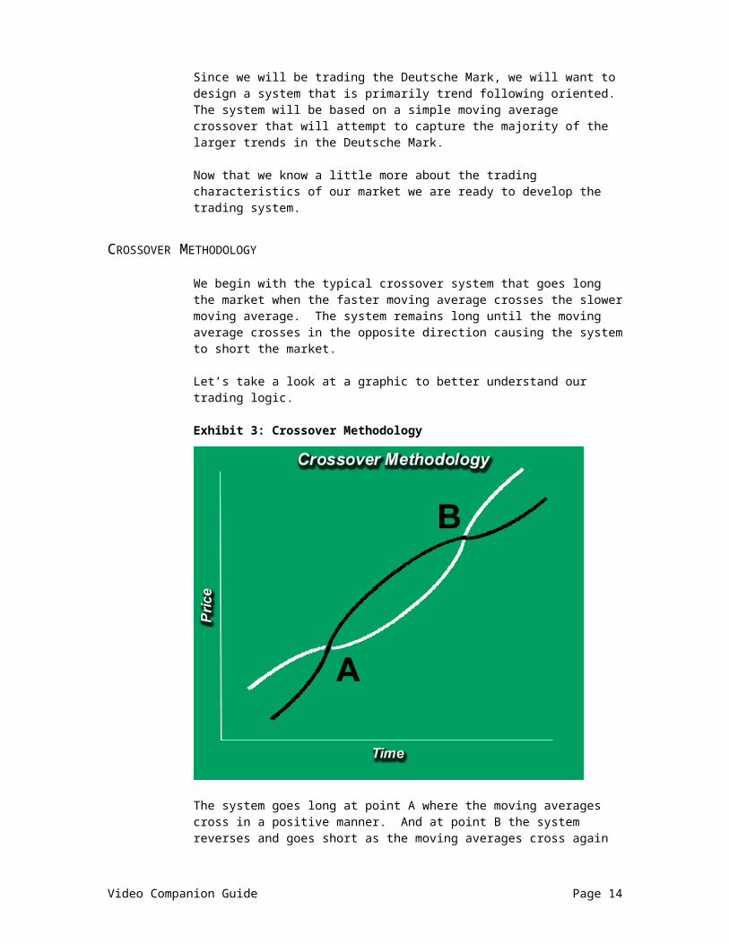


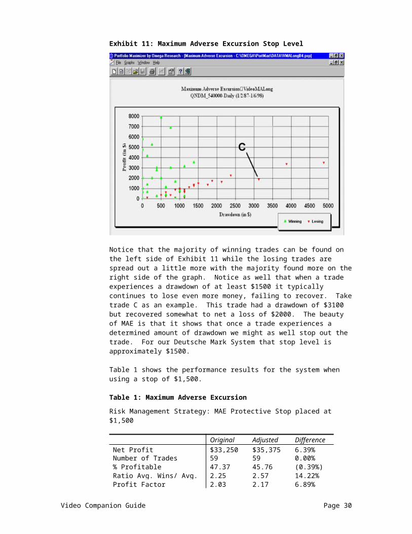
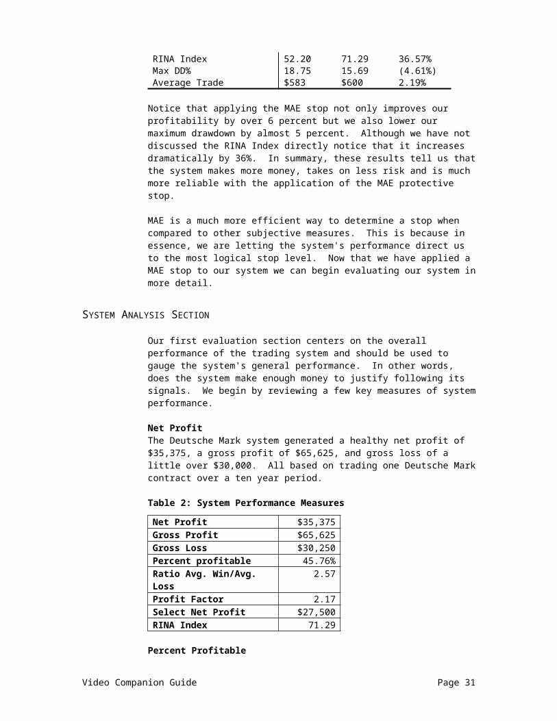


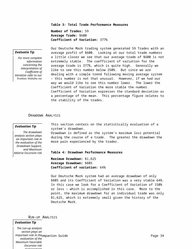


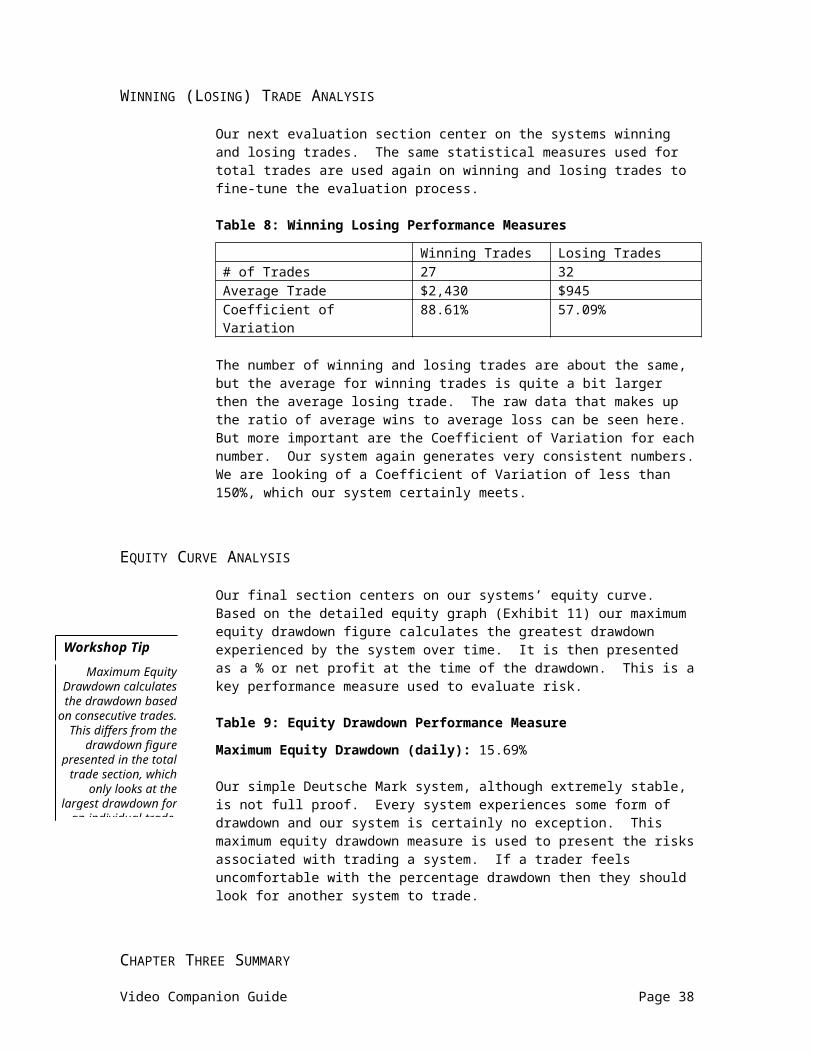


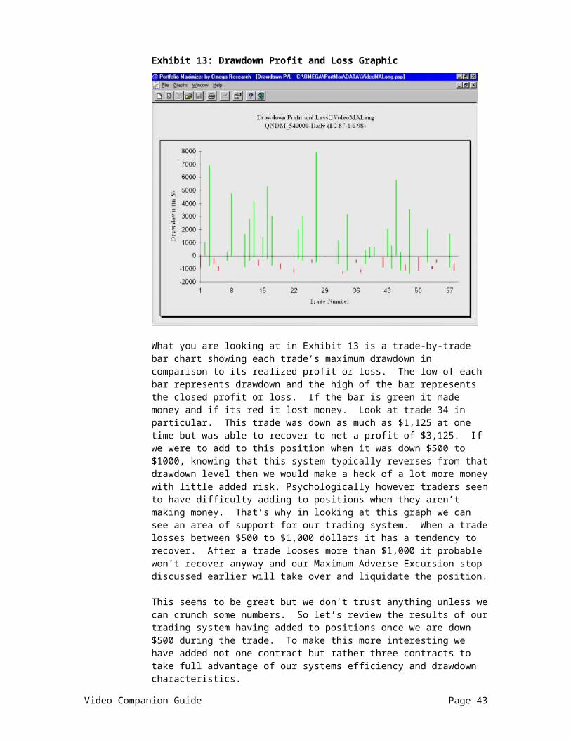


![[XLS]Stockfry.com Yahoo Portfolio Manager UPDATES.xls · Web viewPortfolio Entry Stock Price Details Stock Symbol Help _T1 AutoUpdateOff AutoUpdateOn AutoUpdateStatusCell Company_Name](https://static.documents.pub/doc/80x56/5a9ebbb57f8b9a67178bc8b6/xls-yahoo-portfolio-manager-updatesxlsweb-viewportfolio-entry-stock-price-details.jpg)