JOURNAL OF ECONOMIC DEVELOPMENT 19 Volume 34, Number 1, June 2009 SHORT-RUN AND LONG-RUN EFFECTS OF CURRENCY DEPRECIATION ON THE BILATERAL TRADE BALANCE BETWEEN PAKISTAN AND HER MAJOR TRADING PARTNERS MOHSEN BAHMANI-OSKOOEE AND JEHANZEB CHEEMA * The University of Wisconsin-Milwaukee Previous studies that investigated the short-run (J-curve) and the long-run effects of currency depreciation on the trade balance of Pakistan used aggregate trade data between Pakistan and the rest of the world and provided no evidence of any significant impact. We wonder whether lack of the relation is due to aggregation bias. In this paper, therefore, we go one step further by employing disaggregated data at bilateral level between Pakistan and her 13 major trading partners to determine if we can discover partners whose trade balances react to changes in the real bilateral exchange rate. The results from bounds testing approach are still inconclusive and show that only in half of the cases the real bilateral exchange rate plays a role. Keywords: Bilateral J-Curve, Bounds Testing, Cointegration, Pakistan JEL classification: F31 1. INTRODUCTION A large number of studies that examine short run and long run relationships between exchange rate and trade balance have been conducted in the last few decades. Magee (1973) was one of the very first attempts in the literature to outline possibility of the J-curve phenomenon. He put forward two possible reasons for the existence of a deteriorating trade balance in the wake of currency depreciation. First, there are contract rigidities that take time to wear off. Second, there is a pass-through effect of currency depreciation on domestic prices which may not take place until some time has passed after such depreciation. As a result, favorable effects of exchange rate depreciation may not be immediately visible even though the long run elasticities satisfy the Marshall -Lerner condition. Over the next decades several studies sought to gather evidence for Magee’s * Valuable comments of an anonymous referee are appreciated. Any error, however, is ours.
Transcript
JOURNAL OF ECONOMIC DEVELOPMENT 19 Volume 34, Number 1, June 2009
SHORT-RUN AND LONG-RUN EFFECTS OF CURRENCY
DEPRECIATION ON THE BILATERAL TRADE BALANCE BETWEEN
PAKISTAN AND HER MAJOR TRADING PARTNERS
MOHSEN BAHMANI-OSKOOEE AND JEHANZEB CHEEMA
*
The University of Wisconsin-Milwaukee
Previous studies that investigated the short-run (J-curve) and the long-run effects of
currency depreciation on the trade balance of Pakistan used aggregate trade data between
Pakistan and the rest of the world and provided no evidence of any significant impact. We
wonder whether lack of the relation is due to aggregation bias. In this paper, therefore, we go
one step further by employing disaggregated data at bilateral level between Pakistan and her
13 major trading partners to determine if we can discover partners whose trade balances
react to changes in the real bilateral exchange rate. The results from bounds testing approach
are still inconclusive and show that only in half of the cases the real bilateral exchange rate
1. INTRODUCTION A large number of studies that examine short run and long run relationships between
exchange rate and trade balance have been conducted in the last few decades. Magee (1973) was one of the very first attempts in the literature to outline possibility of the J-curve phenomenon. He put forward two possible reasons for the existence of a deteriorating trade balance in the wake of currency depreciation. First, there are contract rigidities that take time to wear off. Second, there is a pass-through effect of currency
depreciation on domestic prices which may not take place until some time has passed after such depreciation. As a result, favorable effects of exchange rate depreciation may not be immediately visible even though the long run elasticities satisfy the Marshall -Lerner condition.
Over the next decades several studies sought to gather evidence for Magee’s
* Valuable comments of an anonymous referee are appreciated. Any error, however, is ours.
MOHSEN BAHMANI-OSKOOEE AND JEHANZEB CHEEMA 20
hypotheses. Important works from this period include Miles (1979), Bahmani-Oskooee (1985), Flemingham (1988), Meade (1988), Rosenweig and Koch (1988), Noland (1989), Marquez (1991), and Marwah and Klein (1996) among others. These studies experimented with various econometric models, introduced new definitions for the endogenous and exogenous variables, covered different time periods and included a wide range of countries in their analysis. The empirical evidence however remained
mixed. Almost all of the works discussed above relied on either the ordinary least squares (OLS), instrumental variables (IV) or the two-step least squares (2SLS) techniques, all of which are subject to the hazards of spurious correlation unless the time series data under consideration is stationary, thus making their predictions somewhat untenable.1
By late 1980s advancements in econometric theory had allowed researchers to
estimate short run and long run relationships in the presence of non-stationary time series data. The ground-breaking econometric advances in this direction are due to Sims (1980) who pioneered the vector autoregressive (VAR) technique, Engle and Granger (1987) who introduced a two step cointegration test in an error correction modeling framework and, Johansen and Juselius (1990), and Johansen (1991) who proposed cointegration tests for VAR models based on the maximum likelihood method. This
availability of advanced cointegration techniques in time series analysis ushered in a new round of empirical testing from early 1990s to early 2000s. Again, however, the empirical evidence was mixed with some studies supporting the existence of a short run J-curve while others rejecting it. The cointegration techniques discussed above require that all time series variables included in the analysis be integrated of the same order. For models that contain both stationary and non-stationary variables, transformation of the
data may not be a trivial task, not to mention that the results for such transformed variables can be notoriously difficult to interpret.
In the last few years, a new approach to error correction modeling introduced by Pesaran, Shin and Smith (2001) called the bounds testing approach has been employed in time series analysis. This technique can be applied to models in which exact order of integration of variables, though unknown, is not greater than I(1). In other words, the
bounds testing approach can be used in any of the following situations: when all variables are I(0), when all variables are I(1), and when the variables are either I(0) or I(1) or combination of the two. In addition, the bounds testing approach makes it relatively simple to derive the short-run and the long-run effects of one variable on the other. Bahmani-Oskooee and Ratha (2004a) provide a comprehensive review of the literature showing who has applied which technique in testing the J-Curve.
1 For some other studies that deal with trade-related issues see Agbola and Damoense (2005), Alse and
Bahmani-Oskooee (1995), Charos et al. (1996), Du and Zhu (2001), King (1993), Love and Chandra (2005),
Narayan and Narayan (2005), Truett and Truett (2000), Seyoum (2007), and Bahmani-Oskooee and Hegerty
(2007).
SHORT-RUN AND LONG-RUN EFFECTS OF CURRENCY DEPRECIATION 21
Since this paper is about Pakistan, a brief review of the literature about Pakistan’s experience is in order. The number of studies that have included Pakistan in their investigation of the J-curve is small. Many studies investigate only the long run relationship between exchange rate and trade balance while ignoring the J-curve altogether. Furthermore, almost all of the studies that include Pakistan in their analysis either use the OLS, IV or the 2SLS techniques, all of which are prone to the problem of
spurious correlation unless the time series under consideration are stationary, thus casting considerable doubt on their findings. Because of the stationarity problem, at the very least the empirical results in those studies cannot be directly compared with the ones that employ recently developed econometric methods such as the VAR and error-correction modeling technique.
Gylfason and Schmid (1983) used aggregate data on five developed and five less
developed countries and incorporated both demand and supply side effects of real exchange rate depreciation into their model. They found support for a long run relationship between exchange rate and trade balance with an expected increase in trade balance due to a 10% devaluation of Pakistan’s rupee to be equal to 1.3% of Pakistani GNP. However, since the data used were not tested for stationarity, their empirical results are somewhat biased.
Bahmani-Oskooee and Alse (1994) formulated their model following the error correction specification proposed by Engel and Granger (1987). They used aggregate quarterly data from 1970I to 1990IV for 19 developed and 22 less developed countries. Once they controlled for stationarity properties of regression variables, support for co-integration between real exchange rate and trade balance for Pakistan could not be found. It should be noted however that the model used in this study regressed trade
balance directly on the real exchange rate without controlling for other variables such as income. Short run dynamics for countries that failed the co-integration test which included Pakistan were ignored.
Bahmani-Oskooee (1998) employed the Johansen and Juselius maximum likelihood co-integration technique to estimate the well-known Marshall-Lerner condition for six countries using quarterly data over the period 1973I-1990IV. In the results for Pakistan,
the Marshall-Lerner condition which implies that the sum of import and export demand elasticities must add up to more than one was not met. This finding using aggregate data to test the Marshall-Lerner condition is in line with that of Bahmani-Oskooee and Alse (1994) who could not establish cointegration between Pakistani trade balance and the real exchange rate. These findings were, however, contradicted by Aftab and Aurangzeb (2002) who used Johansen and Juselius method and quarterly data over the period
1980-2000 to show that the long-run Marshall-Lerner condition for Pakistan is satisfied. Although their method is an improvement over Bahmani-Oskooee (1998), it may still suffer from aggregation bias as bilateral data for individual trading partners were not employed.
Due to conflicting findings by previous research, as reviewed above, we would like to reconsider the short-run (i.e., the J-curve) and the long-run effects of real depreciation
MOHSEN BAHMANI-OSKOOEE AND JEHANZEB CHEEMA 22
of Pakistani rupee on her trade balance. However, unlike previous research we employ trade data at bilateral level between Pakistan and her 13 major trading partners, a practice originally introduced by Rose and Yellen (1989) for the trade balance between U.S. and her seven trading partners. These 13 partners account for almost 70% of overall trade activity of Pakistan in 2003. In order to get some insight about the relative importance of each partner, we provide these trade shares in Table 1.2
Table 1. Bilateral Trade Flow Between Pakistan and Her Major Trading Partners in 2003
Trading Partners Value of Exports
(Millions of U.S. dollars)
Value of Imports
(Millions of U.S. dollars)
China 447 1,858
France 310 318
Germany 598 672
Hong Kong 472 117
Italy 394 352
Japan 145 838
Korea 259 371
Kuwait 70 918
Malaysia 74 590
Saudi Arabia 448 1,492
U.A.E. 1,013 1,632
U.K. 795 525
U.S.A. 2,528 924
World total 11,283 14,825
Source: Direction of Trade Statistics 2004, International Monetary Fund.
The remaining of the paper is composed of three additional sections. Section 2 presents the model and the method that is based on bounds testing approach to cointegration and error-correction modeling. Empirical results are presented and discussed in sections 3, and formal concluding remarks summarizing the overall findings are presented in section 4. Finally, data sources and definition of variables are cited in an appendix.
2 There is now a growing literature on testing the J-Curve at the bilateral level. Some examples are:
Shirvani and Wilbratte (1997), Bahmani-Oskooee and Kanitpong (2001), Wilson (2001), Bahrumshah (2001),
Bahmani-Oskooee and Goswami (2003), Bahmani-Oskooee and Ratha (2004b, 2004c), Bahmani-Oskooee, et
al. (2005), Bahmani-Oskooee, et al. (2006), and Bahmani-Oskooee, et al. (2008).
SHORT-RUN AND LONG-RUN EFFECTS OF CURRENCY DEPRECIATION 23
2. THE MODEL AND METHOD In assessing the short-run and the long-run effects of changes in the exchange rate on
the trade balance, whether at the aggregate or at the bilateral level, it is a common practice to regress a measure of trade balance directly on real exchange rate while controlling for real income at home and in foreign country. In specifying such a trade
balance model between Pakistan and her trading partner i, we follow the specification by Bahmani-Oskooee and Brooks (1999) and Arora et al. (2003) as outlined by equation (1):
This specification expresses trade balance between Pakistan and trading partner i
( iTB ) defined as the ratio of Pakistan’s nominal imports from trading partner i to her
nominal exports to the same trading partner as a function of Pakistan’s income, tanPakisY ,
income of trading partner i, iY , and the real bilateral exchange rate. We expect an
estimate of b to be positive as an increase in domestic (Pakistan) income generally
leads to an increase in imports. A negative estimate for b is possible if increase in
domestic income reflects expansion in the production of import-substitute goods (Bahmani-Oskooee (1986)). An estimate of g is expected to be negative as an increase
in trading partner’s income leads to higher exports by Pakistan. However, a positive estimate of g is possible if increase in foreign income comes from an expansion in
foreign production of substitutes for Pakistani export goods. Finally, as the appendix
shows iREX is defined in a way that a decrease reflects a real depreciation of Pakistani
rupee. If depreciation is to decrease imports and increase exports, hence improve the trade balance, an estimate of j would be positive
Since the model given in (1) is a long run relationship and the J-curve phenomenon occurs in the short run, it is necessary to modify (1) in order to incorporate the short-run dynamics. A common practice is to express (1) in an error-correction modeling format. We do this by following Pesaran et al.’s (2001) bounds testing approach as in (2):
.loglog
logloglog
loglogloglog
1,41,3
1tan,21,1,
0
,
0
,
0
,
1
,
ttiti
tPakistikti
n
k
k
tki
n
k
kktc
n
k
kkti
n
k
kti
REXY
YTBREX
YYTBTB
udd
ddj
gbha
+++
++D+
D+D+D+=D
--
---
=
=
-
=
-
=
å
ååå
(2)
Pesaran et al. (2001) show that for the error correction specification in (2) there is no
need to test for unit roots as long as all the variables involved are either I(0) or I(1) or combination of the two. In order to justify the retention of lagged level variables, we
MOHSEN BAHMANI-OSKOOEE AND JEHANZEB CHEEMA 24
need to test whether their coefficients are jointly significant. In other words, the null
hypothesis of no cointegration, i.e., 0: 43210 ==== ddddH is tested against the
alternative of 0,0,0,0: 43211 ¹¹¹¹ ddddH . Pesaran et al. (2001) propose applying
the familiar F test with new critical values that they tabulate. An upper bound critical value is tabulated if all variables are I(1) and a lower bound critical value is tabulated if all variables are I(0). An acceptance of the null hypothesis would thus provide evidence
against co-integration while its rejection would provide evidence in support of co-integration. In this set up, the short-run effects of real depreciation is judged by the
estimates of kj ’s. Negative values for lower lags followed by positive values for higher
lags will indeed support the J-curve. The long-run effects of real depreciation are
inferred by the estimate of 4d that is normalized on 1d .
3. EMPIRICAL RESULTS
The error-correction model outlined by Equation (2) is estimated between Pakistan and each of her 13 partners using quarterly data over the period 1980-2003. The first
step is to select the number of lags of first differenced variables. Bahmani-Oskooee and Brooks (1999) have shown that the results of the F test will depend on the number of lags. In order to see how the F test reacts to number of lags selected, as a starting exercise two, four, six and eight lags are introduced. The calculated F values for these models are presented in Table 2. As can be seen from the results, the F values are sensitive to the number of lags imposed. As we move from 2 lags to 8 lags, the number
of significant cases at 10% level of significance drops from 11 to just 2.
Table 2. The Results of the F Test at Different Lags Trading Partners 2 lags 4 lags 6 lags 8 lags China 12.0122 3.8139 3.5187 1.9880
France 6.4872 3.6668 3.7595 3.5733
Germany 4.5402 4.2837 2.0405 1.6201
Hong Kong 4.2470 2.9708 1.9853 1.4031
Italy 2.8284 1.8739 1.1373 1.8288
Japan 4.1240 3.7934 1.2314 1.1215
Korea 2.3109 1.0972 2.7453 1.3999
Kuwait 6.6424 5.4359 3.2146 1.8568
Malaysia 4.1733 2.7942 1.9837 1.2673
Saudi Arabia 4.3051 3.3158 4.0083 3.5524
U.A.E. 4.5701 2.8070 0.9683 1.1089
U.K. 6.8756 4.5153 3.6117 3.3482
U.S.A. 6.3129 3.2869 3.9560 2.2607
Note: Critical values of F statistic at 5% and 10% levels of significance are 4.01 and 3.52 respectively.
Source: These are taken from Pesaran, Shin and Smith (2001).
SHORT-RUN AND LONG-RUN EFFECTS OF CURRENCY DEPRECIATION 25
Given such sensitivity of test results to number of lags, following Bahmani-Oskooee and Gelan (2006) we rely on some information criterion in order to select the optimal number of lags and carry the F test at optimum lags. The two criteria considered in this study are the Akaike Information Criterion (AIC) and the Schwarz Bayesian Criterion (SBC). F test results and number of optimal lags for models using AIC and SBC are presented in Table 3. These results show that the number of significant cases at 10%
level of significance for models with AIC-selected lags is 11 while this number increases to 12 for models using SBC-selected lags. Furthermore, all the F values that are significant at 10% level of significance under both AIC and SBC, unlike Table 2 results, are also significant at 5% level of significance.
Table 3. F Statistics at AIC and SBC-Selected Optimal Lags
Trading Partners AIC
Optimal lags
F Statistic at
AIC-Selected
Optimal Lags
SBC
Optimal Lags
F Statistic at
SBC-Selected
Optimal Lags
China 3,0,3,0 8.2941 1,0,0,0 30.3398
France 0,1,0,0 19.4358 0,1,0,0 19.4358
Germany 0,3,0,0 10.2310 0,0,0,0 9.7009
Hong Kong 0,3,7,0 9.6113 0,0,0,0 10.0022
Italy 6,0,0,2 1.3540 0,0,0,0 5.3217
Japan 0,3,0,0 11.2341 0,0,0,0 6.9143
Korea 2,0,1,0 2.4253 2,0,0,0 2.3155
Kuwait 2,0,4,3 7.2734 0,0,1,0 18.5362
Malaysia 2,0,1,0 5.0955 0,0,0,0 9.9226
Saudi Arabia 6,7,8,0 4.6881 0,0,3,0 6.8545
U.A.E. 1,0,0,1 4.7006 0,0,0,0 12.7654
U.K. 0,0,0,1 13.5272 0,0,0,1 13.5272
U.S.A. 4,0,0,0 6.0962 0,0,0,0 15.2139
Notes: a) Critical values of F statistic at 5% and 10% levels of significance are 4.01 and 3.52 respectively.
These are taken from Pesaran, Shin and Smith (2001). b) The number of lags follows the specification in
model (2). Thus 3,0,3,0 for China means that three lags were imposed on iTBlogD , zero lags on
tanlog PakisYD , three lags on iYlogD , and zero lags on iREXlogD .
It should be noted here however that Table 3 results are sensitive to lag selection
criterion. This can be observed in case of Italy for which the calculated F value is not significant when AIC is used but becomes significant under SBC. For this reason, and because of additional co-integration analysis presented later in this work, it is decided to keep the lagged values in all cases even where F test is not significant.
MOHSEN BAHMANI-OSKOOEE AND JEHANZEB CHEEMA 26
(Table 4 is here.)
SHORT-RUN AND LONG-RUN EFFECTS OF CURRENCY DEPRECIATION 27
In order to assess the J-curve or the short-run effects of real depreciation, we next report the coefficient estimates obtained for 1log -D tREX variables. Since AIC
criterion chooses longer lags, here we restrict ourselves to reporting AIC based results. These results are reported in Table 4.
As indicated before, existence of the J-curve can be inferred by looking at the
coefficient estimates of itREX -D log . Negative coefficients followed by positive ones
would support the J-curve. The results in Table 4 suggest that these coefficient estimates
follow the J-curve pattern only for Italy even though some of these estimates are not significant. Although results in Table 4 do not support the existence of J-curve, there is at least one significant coefficient at the 10% level in the cases of China, Italy, Korea, Kuwait, U.A.E., and the U.K., suggesting that importance of real exchange rate as a determinant of trade balance in the short run cannot be completely ignored.3 The next question is in how many of these countries, the short-run significant effects last into the
long run. To this end, we report in Table 5 and 6 estimates of 32 ,dd and 4d
normalized on 1d from both AIC based and SBC based models.
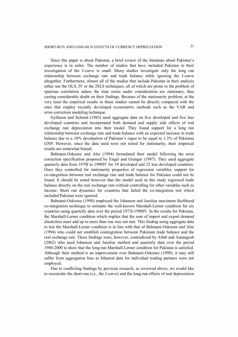
Table 5 results show that the coefficient on real exchange rate is positive in twelve out of thirteen cases, and is significant and positive for six cases at 5% level of significance. These results signal that a long run relationship between real exchange rate and trade balance cannot be ignored. The coefficient on Pakistani income is positive for
six of the trading partners but is significant for only five at 5% level of significance. For Hong Kong and Japan, real Pakistani income has a negative but significant coefficient. These results provide support for a long term relationship between real Pakistani income and her trade balance. Coefficients on incomes of trading partners have the correct sign and significance at 5% level of significance for only two partners, Germany and U.K. For Kuwait and U.A.E. the coefficients are significant but have a positive sign.
The situation in Table 6 is almost similar with the only difference that Saudi Arabia now has a negative coefficient on real exchange rate and the coefficient for Japan is no longer significant. For five countries the coefficients are positive and significant, again suggesting that a long run relationship between real exchange rate and trade balance cannot be ruled out. The coefficient on real Pakistani income is positive for more than half of the trading partners but is significant and positive for only three at 5% level of
significance. Two trading partners have a negative but significant coefficient on real Pakistani income. Overall these results provide support for a long run relationship between Pakistani income and her trade balance. Coefficients on income of trading partner have the correct sign and significance at 5% level of significance for three partners. For four other partners the coefficients are significant but have a positive sign. Again, these results provide support for a long run relationship between partner’s
income and own trade balance.
3 Results from SBC-selected models showed a similar story with scarce support for the J-curve.
MOHSEN BAHMANI-OSKOOEE AND JEHANZEB CHEEMA 28
Table 5. Long-run Coefficient Estimates of Models Using AIC Lag Selection
SHORT-RUN AND LONG-RUN EFFECTS OF CURRENCY DEPRECIATION 29
Italy 6.18 -0.41 -0.18 0.07
(0.60) (0.62) (0.28) (1.37)
Japan -1.92 -1.18 0.91 1.66
(0.15) (3.08) (1.08) (1.59)
Korea -79.46 0.25 4.71 7.49
(1.37) (0.26) (1.32) (1.50)
Kuwait -34.99 0.42 4.6 2.36
(2.82) (0.48) (9.92) (2.31)
Malaysia -3.78 0.92 0.14 1.43
(0.37) (1.49) (0.23) (1.06)
Saudi Arabia 3.77 -0.83 0.36 -0.59
(0.31) (1.73) (0.45) (0.58)
U.A.E. -6.92 -0.91 2.1 1.5
(0.72) (1.40) (3.91) (3.45)
U.K. 25.22 -0.18 -1.65 0.9
(6.85) (0.89) (9.27) (5.72)
U.S.A. 11.03 1.58 -1.78 0.17
(0.94) (3.88) (2.94) (0.61) Note: Figures in parentheses are t-values.
In the next stage of this analysis, estimates of 32 ,dd and 4d normalized on 1d
are used to calculate the linear combination of 1,log -tiTB , logYPakistan, t-1, 1,log -tiY , and
1,log -tiREX as a new series, denoted by 1, -tiECM . After replacing the linear combination
of lagged level variables by 1-tECM and after imposing the optimum lags, we estimate
(2) one more time. A significantly negative coefficient obtained for 1-tECM not only
supports cointegration but also adjustment toward equilibrium. These results are also
reported in Table 4. As can be seen, all 1, -tiECM coefficients are negative and
significant with Italy being the only exception.4
Although 1, -tiECM coefficient estimates reported in Table 4 are highly significant
and constitute enough evidence to support endogeneity of iTBlog , it is worthwhile to
test the possibility of any of the other three variables in (1) being endogenous.5 Following Boyd et al. (2003) and Bahmani-Oskooee and Wang (2006), this is done by
4 It should be mentioned that SBC-based models yielded the same results. 5 In any error-correction model, one interpretation of a significant lagged error-correction term is that the
right-hand-side variables in the long-run model cause the dependent variable, implying that the right-hand-
side variables are exogenous where as the dependent variable is endogenous. For more on this see Jones and
Joulfaian (1991, p. 150).
MOHSEN BAHMANI-OSKOOEE AND JEHANZEB CHEEMA 30
re-estimating (2) after interchanging iTBlogD , the dependent variable in (2) with the
remaining three exogenous variables one by one. The 1-tECM coefficient estimates
from these additional models are reported in Table 7. These results show strong support for endogeneity of real exchange rate with all 13 coefficients being negative and significant at 5% level of significance. There is also mixed support for the endogeneity of real income of Pakistan and that of her trading partners. In short, the assumption of
right hand side variables in (1) being completely exogenous seems untenable.6
Table 7. Coefficient Estimates of 1, -tiECM with Different Dependent Variables Under AIC
Trading partners
Dependent
variable TBlogD
Dependent
variable REXlogD
Dependent
variable logD YPakistan
Dependent
variable
PartnerYlogD
China -1.11 -0.38 0.04 0.01
(5.17) (3.73) (0.53) (0.30)
France -0.82 -0.12 -0.08 -0.07
(7.56) (2.73) (0.72) (2.40)
Germany -0.67 -0.18 -0.24 -0.07
(6.34) (3.31) (2.59) (1.63)
Hong Kong -0.71 -0.18 -0.14 -0.38
(6.28) (3.15) (1.33) (4.90)
Italy -0.14 -0.11 0.06 -0.07
(0.92) (2.49) (0.81) (1.82)
Japan -0.52 -0.25 -0.00 -0.40
(5.96) (3.18) (0.01) (6.40)
Korea -0.17 -0.25 -0.13 -0.18
(2.47) (3.16) (2.70) (2.06)
Kuwait -0.91 -0.32 -0.60 -0.18
(4.96) (4.57) (4.03) (1.55)
Malaysia -0.53 -0.35 -0.22 -0.05
(4.11) (4.30) (3.82) (1.54)
Saudi Arabia -0.56 -0.38 -0.02 -0.06
(4.35) (3.47) (0.29) (1.40)
6 Note that Bahmani-Oskooee and Tanku (2006, p. 261) have argued that the issue is not as serious as it
sounds, mostly because lagged values in the model could be considered as instruments for current values
which amounts to treating each variable as endogenous.
SHORT-RUN AND LONG-RUN EFFECTS OF CURRENCY DEPRECIATION 31
U.A.E. -0.59 -0.12 -0.29 -0.02
(4.86) (2.71) (2.13) (0.34)
U.K. -0.80 -0.36 -0.15 -0.15
(7.41) (4.02) (1.66) (3.73)
U.S.A. -0.61 -0.43 -0.15 -0.10
(4.36) (4.65) (1.12) (2.06)
Note: Figures in parentheses are t-values.
Table 8. Johansen’s Maximum Likelihood Results with AIC-selected VAR Order
Note: Number of co-integrating vectors is given by r.
In order to allow the feedback effects among the variables in (1), Johansen’s
co-integration approach is adopted. After confirming through various tests, including the ADF unit root test, the I(1) property of our variables, the next step in the Johansen’s co-integration analysis is to calculate max-l and trace statistics that will help us
identify the number of co-integrating vectors.7 Once again in selecting the optimum lags,
7 China, Italy and U.A.E. have at least one I(0) series and thus the results for these countries should be
interpreted with some caution.
MOHSEN BAHMANI-OSKOOEE AND JEHANZEB CHEEMA 32
we rely upon the AIC criterion. Note that following Cheung and Lai (1993, p. 317), the two statistics are adjusted for the number of observations T, number of lags n, and the number of variables in the co-integrating space m. The adjustment factor is (T-nm)/T. Thus, max-l and trace statistics that are reported in Table 8 are the original figures
multiplied by the adjustment factor.
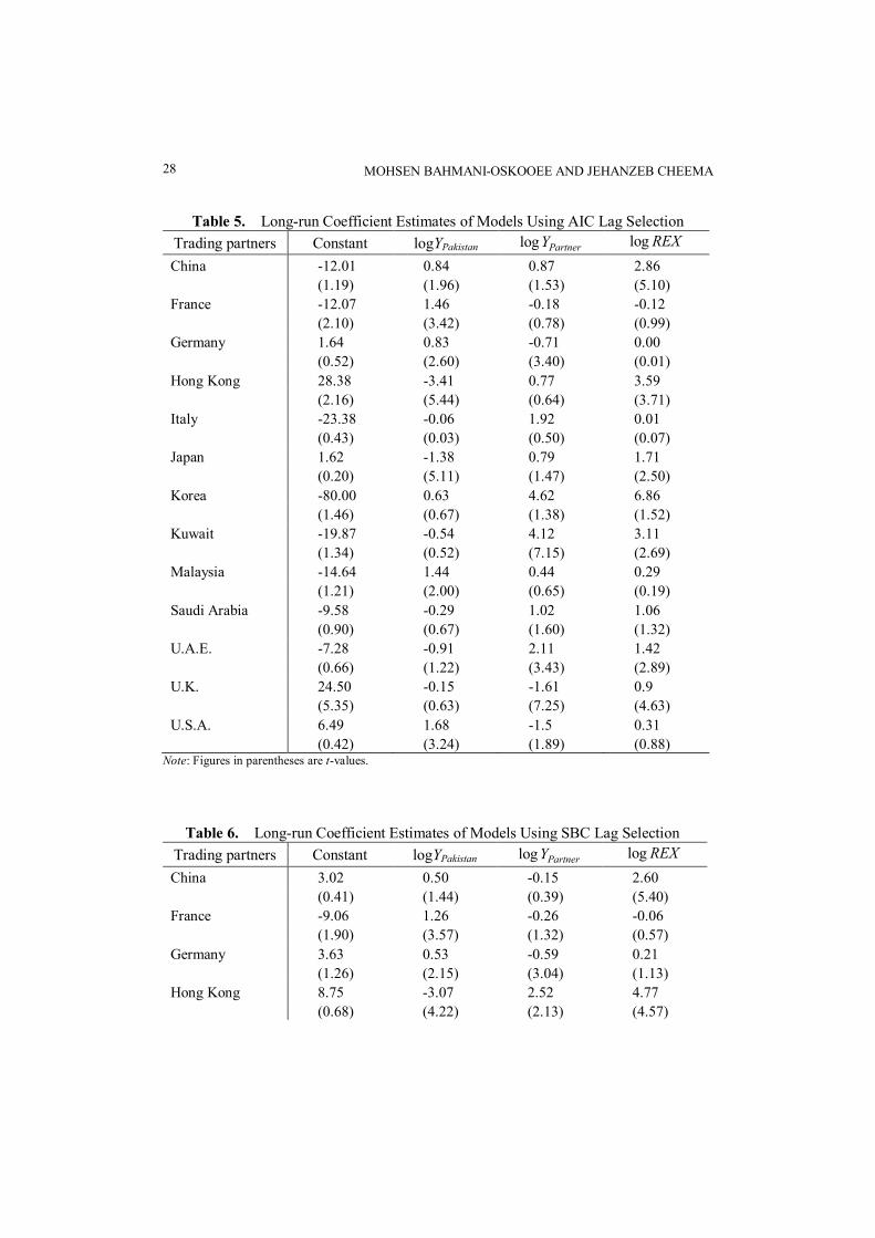
Table 9. The Maximum Likelihood Estimate of Each Co-integrating Vector Under AIC
Notes: The critical values of 2c statistic are given in parentheses. At 1%, 5% and 10% levels of
significance with 1 degree of freedom these critical values are 6.63, 3.84 and 2.71.
SHORT-RUN AND LONG-RUN EFFECTS OF CURRENCY DEPRECIATION 33
(Figure 1 is here.)
MOHSEN BAHMANI-OSKOOEE AND JEHANZEB CHEEMA 34
(Figure 1 is here. - continued)
SHORT-RUN AND LONG-RUN EFFECTS OF CURRENCY DEPRECIATION 35
(Figure 1 is here. - continued)
MOHSEN BAHMANI-OSKOOEE AND JEHANZEB CHEEMA 36
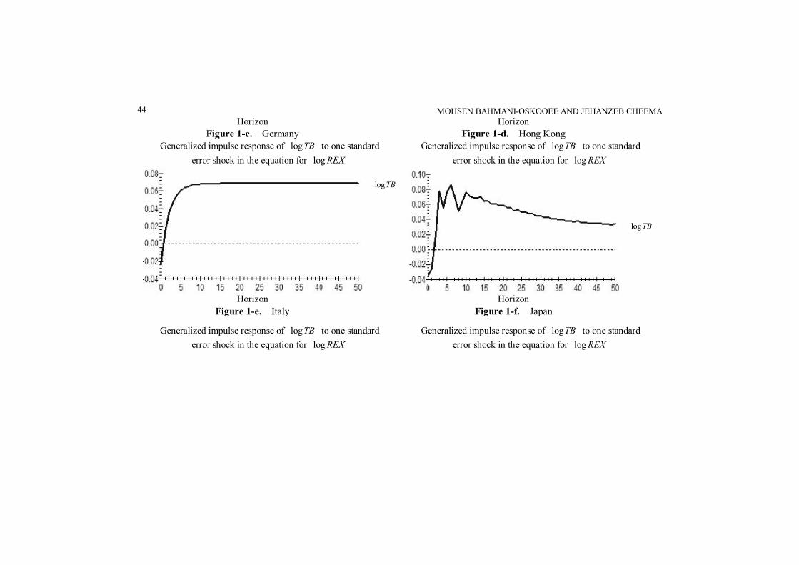
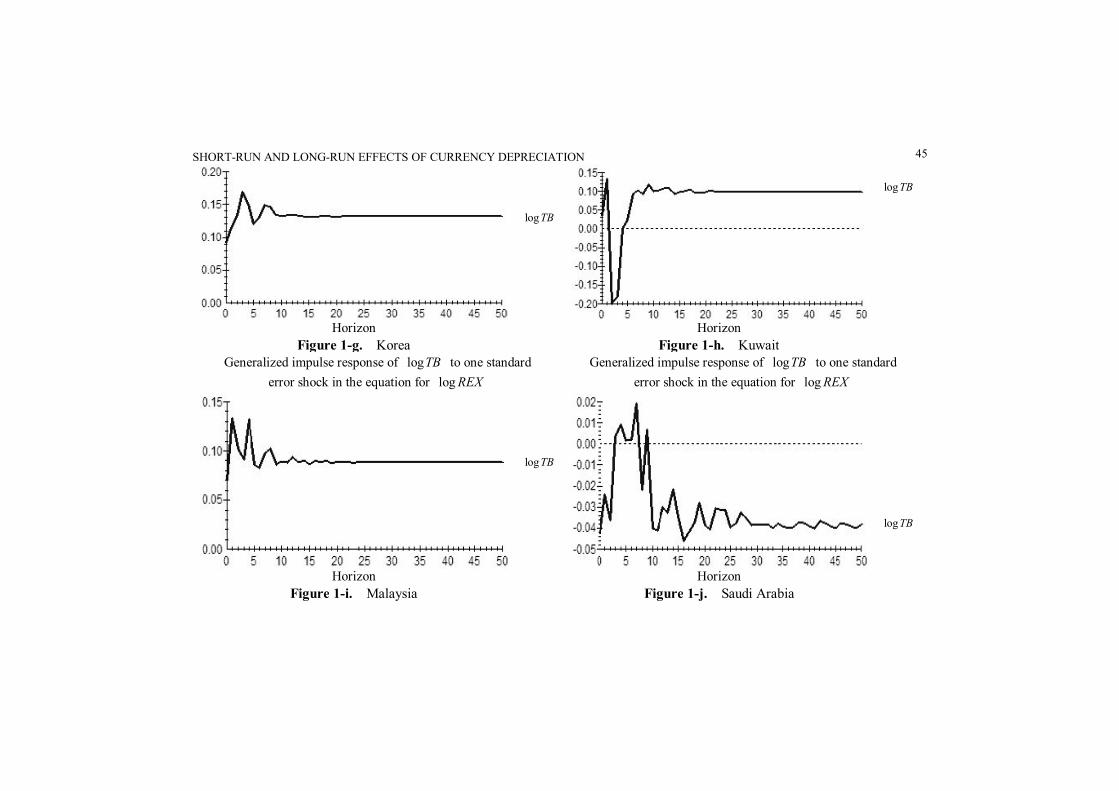
Figure 1. Generalized Impulse Response of TBlog to One Standard Error Shock
in the Equation for REXlog Under AIC
Table 8 figures show that null of no co-integration is rejected at 10% level of
significance only for Hong Kong, Italy, U.A.E. and U.S.A. using either max-l or
trace test. Also, using either test, there is no evidence for the existence of more than one vector except in case of U.A.E. and U.S.A. Based on these results it is assumed that for all countries at least one co-integrating vector exists. The results for the first vector are
reproduced in Table 9 along with calculated value of the 2c statistic for likelihood
ratio test of exclusion of corresponding variable in parentheses below the maximum likelihood estimates. Notice that the maximum likelihood estimates are normalized on
the coefficient of iTBlog which is set equal to -1.
It can be seen from Table 9 that iREXlog has a significant coefficient for Hong
Kong and Korea at 5% level of significance, with Italy added to the list at 10% level. However, only the coefficient for Italy carries the correct sign. With SBC lag selection criterion (results not reported here but available upon request) we can further expand the list of trading partners to include China, Hong Kong, Japan, U.A.E. and U.K with both
significant and positive coefficients on iREXlog , and Saudi Arabia with a significant
but negative coefficient at 10% level of significance. These results are similar to those obtained from the bounds testing approach.
Following Halicioglu (2007), as a final step, the existence of J-curve is tested under
this feedback scenario using Johansen’s full information estimates for each trading
partner by tracing out the generalized impulse response function of iTBlog to one
standard error shock in the equation for iREXlog . Since increase in iREXlog represents
real exchange rate appreciation, an inverse J shape of the impulse response function
Generalized impulse response of TBlog to one standard
error shock in the equation for REXlog
TBlog
Horizon Figure 1-m. U.S.A
SHORT-RUN AND LONG-RUN EFFECTS OF CURRENCY DEPRECIATION 37
would constitute evidence for the existence of the J-curve. Graphs of impulse response functions for all trading partners are presented in Figure 1. None of these plots clearly support the inverse J-curve.
4. SUMMARY AND CONCLUSION In the last few decades numerous studies have sought evidence in support of the
J-curve. The results however have not been conclusive. A recent trend in literature has been to employ disaggregated bilateral data between a country and her major trading partners in order to avoid the aggregation bias that can be present when aggregated data is used.
Previous research on Pakistan relied on aggregated data for J-curve related studies. This study went one step further and employed disaggregated bilateral data between Pakistan and her 13 largest trading partners in order to test the short-run (J-curve) and the long-run effects of real depreciation of Pakistani rupee. The two econometric techniques used for this purpose were the bounds testing approach and Johansen’s co-integration approach. Two information criteria (Akaike Information Criterion and
Schwarz Bayesian Criterion) for model selection were employed and a number of diagnostic tests were conducted in order to ensure the appropriateness of econometric results.
The bounds testing approach provided some evidence of short run effect of real exchange rate on trade balance. However these short run dynamics were inconsistent with the J-curve hypothesis. The long run results showed evidence of a positive and
significant relationship between real exchange rate and trade balance in almost half of the trading partners in the sample using the bounds testing approach. The list included China, Hong Kong, Japan, Kuwait, and U.A.E. One policy implication of our findings is that not all trading partners are affected by real depreciation of Pakistani currency. The two largest trading partners, i.e., China and U.A.E. will be hurt by depreciation of Pakistani rupee. Johansen’s co-integration approach did not provide much evidence in
support of the J-curve nor any evidence of a significant long-run impact of the real exchange rate on bilateral trade balance.
APPENDIX. Data Definition and Sources Quarterly data over 1980Q1-2003Q4 period was used for empirical analysis and
came from World Development Indicators (World Bank, 2004 CD-ROM), International Financial Statistics (International Monetary Fund; online CD-ROM) and Direction of Trade Statistics (International Monetary Fund; 2004 CD-ROM).
MOHSEN BAHMANI-OSKOOEE AND JEHANZEB CHEEMA 38
Variables:
1. =iTB Pakistan’s trade balance with her trading partner i. It is calculated as
Pakistan’s nominal imports from trading partner i divided by her nominal exports to the
same trading partner.
2. =iY measure of real GDP for country i. Where unavailable, quarterly GDP
figures were generated following Bahmani-Oskooee (1986). tanPakisY is Pakistani real
GDP.
3. =iREX bilateral real exchange rate between Pak Rs. and the trading partner i’s
currency. NEXPPREX iPakisi ´= )/( tan , where tanPakisP and iP are the price levels
(CPI used as proxy) in Pakistan and in trading partner i, and iNEX is the bilateral
nominal exchange rate expressed as number of units of trading partner i’s currency per Pak Rs.
REFERENCES
Aftab, Z., and Aurangzeb (2002), “The Long Run and Short Run Impacts of Exchange
Rate Devaluation on Pakistan’s Trade Performance,” The Pakistan Development Review, 41(3), 277-286.
Agbola, F.W., and Maylene Y. Damoense (2005), “Time-series Estimation of Import Demand Functions for Pulses in India,” Journal of Economic Studies, 32, 146-157.
Alse, J., and M. Bahmani-Oskooee (1995), “Do Devaluations Improve or Worsen the Terms of Trade?” Journal of Economic Studies, 22, 16-25.
Arora, S., Bahmani-Oskooee, M. and G. Goswami (2003), “Bilateral J-Curve Between India and Her Trading Partners,” Applied Economics, 35(9), 1037-1041.
Bahmani-Oskooee, M. (1985), “Devaluation and the J-Curve: Some Evidence from LDCs,” The Review of Economic and Statistics, 67(3), 500-504.
_____ (1986), “Determination of International Trade Flows: The Case of Developing Countries,” Journal of Development Economics, 20(1), 107-123.
_____ (1998), “Cointegration Approach to Estimate the Long-Run Trade Elasticities in LDCs,” International Economic Journal, 12(3), 89-96.
Bahmani-Oskooee, M., and J. Alse (1994), “Short-Run versus Long-Run Effects of Devaluation: Error-Correction Modeling and Cointegration,” Eastern Economic
Journal, 20(4), 453-464. Bahmani-Oskooee, M., and T.J. Brooks (1999), “Bilateral J-curve Between U.S. and Her
Trading Partners,” Weltwirtschaftliches Archiv, 135(1), 156-165. Bahmani-Oskooee, M., and T. Kantipong (2001), “Bilateral J-Curve Between Thailand
and Her Trading Partners,” Journal of Economic Development, 26, 107-117. Bahmani-Oskooee, M., and G. Goswami (2003), “A Disaggregated Approach to Test the
SHORT-RUN AND LONG-RUN EFFECTS OF CURRENCY DEPRECIATION 39
J-Curve Phenomenon: Japan vs. Her Major Trading Partners,” Journal of Economics and Finance, 27, 102-113.
Bahmani-Oskooee, M., and A. Ratha (2004a), “The J-Curve: A literature Review,” Applied Economics, 36(13), 1377-1398.
_____ (2004b), “The J-Curve Dynamics of U.S. Bilateral Trade,” Journal of Economics and Finance, 28, 32-38.
_____ (2004c), “Dynamics of U.S. Trade with Developing Countries,” Journal of Developing Areas, 37, 1-11.
Bahmani-Oskooee, M., and A. Gelan (2006), “Black Market Exchange Rate and the Productivity Bias Hypothesis,” Economic Letters, 91(2), 243-249.
Bahmani-Oskooee, M., and A. Tanku (2006), “Black Market Exchange Rate, Currency Substitution and the Demand for Money in LDCs,” Economic Systems, 20, 249-263.
Bahmani-Oskooee, M., and Y. Wang (2006), “The J Curve: China versus Her Trading Partners,” Bulletin of Economic Research, 58(4), 323-343.
Bahmani-Oskooee, M., and S.W. Hegerty (2007), “Exchange Rate Volatility and Trade Flows: A Review Article,” Journal of Economic Studies, 34, 211-255.
Bahmani-Oskooee, M., C. Economidou, and G. Goswami (2006), “Bilateral J-Curve Between the U.K. vis-à-vis Her Major Trading Partners,” Applied Economics, 38,
879-888. Bahmani-Oskooee, M., G. Goswami, and B. Talukdar (2005), “The Bilateral J-Curve:
Australia versus Her 23 Trading Partners,” Australian Economic Papers, 44, 110-120. _____ (2008), “The Bilateral J-Curve: Canada versus Her 20 Major Trading Partners,”
International Review of Applied Economics, 22, 93-104. Baharumshah, A.Z. (2001), “The Effect of Exchange Rate on Bilateral Trade Balance:
New Evidence from Malaysia and Thailand,” Asian Economic Journal, 15, 291-312. Boyd, D., G.M. Caporale, and R. Smith (2001), “Real Exchange Rate Effects on the
Balance of Trade: Cointegration and the Marshall-Lerner Condition,” International Journal of Finance and Economics, 6, 187-200.
Charos, E.N., E.O. Simos, and A.R. Thompson (1996), “Exports and Industrial Growth: A New Framework and Evidence,” Journal of Economic Studies, 23, 18-31.
Cheung, Y., and K. Lai (1993), “Finite-Sample Sizes of Johansen’s Likelihood Ratio Tests for Cointegration,” Oxford Bulletin of Economics and Statistics, 55(3), 313-328.
Du, H., and Z. Zhu (2001), “The Effect of Exchange-Rate Risk on Exports: Some Additional Empirical Evidence,” Journal of Economic Studies, 28, 106-121.
Engle, R.F., and C.W.J. Granger (1987), “Co-Integration and Error Correction:
Representation, Estimation, and Testing,” Econometrica, 55(2), 251-276. Felmingham, B.S. (1988), “Where is the Australian J-Curve?” Bulletin of Economic
Research, 40(1), 43-56. Gylfason, T., and M. Schmid (1983), “Does Devaluation Cause Stagflation?” The
Canadian Journal of Economics, 16(4), 641-654.
MOHSEN BAHMANI-OSKOOEE AND JEHANZEB CHEEMA 40
Halicioglu, F. (2007), “The J-Curve Dynamics of Turkish Bilateral Trade: A Cointegration Approach,” Journal of Economic Studies, 34, 103-119.
Johansen, S. (1991), “Estimation and Hypothesis Testing of Cointegration Vectors in Gaussian Vector Autoregressive Models,” Econometrica, 59(6), 1551-1580.
Johansen, S., and K. Juselius (1990), “Maximum Likelihood Estimation and Inference on Cointegration: With Applications to the Demand for Money,” Oxford Bulletin of
Economics and Statistics, 52(2), 169-210. Jones, J.D., and D. Joulfaian (1991), “Federal Government Expenditures and Revenues
in the Early Years of the American Republic: Evidence from 1792 to 1860,” Journal of Macroeconomics, 13, 133-155.
King, A. (1993), “The Functional Form of Import Demand: The Case of UK Motor Vehicle Imports, 1980-90,” Journal of Economic Studies, 20, 36-50.
Love, J., and R. Chandra (2005), “Testing Export-led Growth in South Asia,” Journal of Economic Studies, 32, 132-145.
Magee, S.P. (1973), “Currency Contracts, Pass Through and Devaluation,” Brooking Papers on Economic Activity, 1973(1), 303-325.
Marquez, J. (1991), “The Dynamics of Uncertainty or the Uncertainty of Dynamics: Stochastic J-Curves,” Review of Economics and Statistics, 73(1), 125-133.
Marwah, K., and L.R. Klein (1996), “Estimation of J-Curves: United States and Canada,” The Canadian journal of Economics, 29(3), 523-539.
Meade, E.E. (1988), “Exchange Rate, Adjustment, and the J-Curve,” Federal Reserve Bulletin, 74(10), 633-644.
Miles, M.A. (1979), “The Effects of Devaluation on the Trade Balance and the Balance of Payments: Some New Results,” The Journal of Political Economy, 87(3),
600-620. Narayan, S., and P.K. Narayan (2005), “An Empirical Analysis of Fiji’s Import Demand
Function,” Journal of Economic Studies, 32, 158-168. Noland, M. (1989), “Japanese Trade Elasticities and the J-Curve,” Review of Economic
and Statistics, 71(1), 175-179. Pesaran, M.H., Y. Shin, and R.J. Smith (2001), “Bounds Testing Approaches to the
Analysis of Level Relationships,” Journal of Applied Econometrics, 16(3), 289-326. Rose, A.K., and J.L. Yellen (1989), “Is There a J-curve?” Journal of Monetary
Economics, 24(1), 53-68. Rosenweig, J.A., and P.D. Koch (1988), “The U.S. Dollar and the Delayed J-Curve,”
Economic Review, 73(4), 2-15. Seyoum, B. (2007), “Export Performance of Developing Countries Under the Africa
Growth and Opportunity Act; Experience from US Trade with Sub-Saharan Africa,” Journal of Economic Studies, 34, 515-533.
Shirvani, H., and B. Wilbratte (1997), “The Relation Between the Real Exchange Rate and the Trade Balance: An Empirical Reassessment,” International Economic Journal, 11(1), 39-49.
Sims, C.A. (1980), “Macroeconomics and Reality,” Econometrica, 48(1), 1-48.
SHORT-RUN AND LONG-RUN EFFECTS OF CURRENCY DEPRECIATION 41
Truett, L.J., and Dale B.T. (2000), “The Demand for Imports and Economic Reform in Spain,” Journal of Economic Studies, 27, 182-199.
Wilson, P. (2001), “Exchange Rates and the Trade Balance for Dynamic Asian Economies-Does the J-Curve Exist for Singapore, Malaysia and Korea?” Open Economies Review, 12, 389-413.
Mailing Address: The Center for Research on International Economics and Departmenr of Economics, The University of Wisconsin-Milwaukee, Milwaukee, WI 53201. Tel: 414-229-4334. E-mail: [email protected].
Received December 6, 2007, Revised May 13, 2008, Accepted September 3, 2008.
MOHSEN BAHMANI-OSKOOEE AND JEHANZEB CHEEMA 42
Table 4. Coefficient Estimates for itREX -D log Under AIC Lag Selection