12
Stochastical Immunological Layer Optimizer SILO II

Stochastical Immunological Layer Optimizer
SILO II

Stochastical ImmunologicalLayer Optimizer
SILO IIBio-inspired computing is a field which helps us solve complex problems using computational methods ob-served in nature. For example, Artificial Intelligence al-gorithms and models such as Neural Networks, Genetic Algorithms and Particle Swarm Optimization, are very useful in industrial process control and optimization. One of the newest fields in bio-inspired computing are methods inspired by the operation of immune systems of living creatures. Characteristic features of Artificial Immune Systems are on-line learning and effective ad-aptation. These features are much desired in solutions which perform on-line industrial process optimization and control. Below we present SILO II - a new immune inspired optimizer of industrial processes, which has demonstrated with stunning success to provide high efficiency gains in power plants in USA, South Korea, Taiwan and Poland.
SILO II is one of the Emerson SmartProcess applica-tion modules used in large-scale industrial processes for advanced control and optimization. The main ap-plication of the SILO II system is combustion pro-cess optimization. Heat and electricity producers can minimize NO
X, CO and SO
2 emissions and increase
generation efficiency. SILO II also can be used to in-crease plant controllability. Therefore, costs related to the power generation process itself, and to emis-sions control regulations are reduced. Furthermore, when using SILO II, companies may avoid the higher costs of emission mitigation systems allowing for substantial increases in their infrastructure efficiency. SILO II could also be used for FGD, SCR and SNCR optimization.
SILO II system performs an on-line optimization of MIMO (Multi Input Multi Output) industrial processes. It is responsible for:
• Maximization of income that is related with output product,
• Minimization of costs which are related with fuel costs and penalties for air pollution.
The SILO II economical calculation module helps to de-fine optimization goals, that assure the best economical profits. In the case of combustion processes in power boilers, SILO II increases process efficiency, reduces NO
X, CO and SO
2 emissions, reduces LOI (Loss of Igni-
tion) and decreases unit heat rate.
SILO II base information
SILO II is a completely new solution for industrial pro-cess optimization. This new approach is based on analogy with the immune systems of living creatures. Other advanced process control and optimization solu-tions are based on a large, sophisticated models, that are difficult to obtain, maintain and tune. SILO II uses a different approach. It gathers portions of knowledge (B cells) about the process, and uses selected portions of knowledge to forecast plant behavior in the close neighborhood of the current process operating point. Such an approach used within the SILO II system has some unique features:
On-line learning of a process based on current meas-urements
Comment: SILO II learns static process responses for a given control change. In particular it stores packets of information which in analogy to the immune system are like B cells. These packets are used by the optimiza-tion module to create a direct model of inner process dependencies in the neighborhood of the current pro-cess operating point. Moreover SILO II is able to gather knowledge about the process based on historical data that may be stored within a DCS system.
Direct and fast adaptation to current process state
Comment: Using its own knowledge base, SILO II is able to identify de-pendences between process inputs and outputs for each analyzed pro-cess operating point. It is a brand new approach in process non-line-
arity handling. Based on the B cell specialized knowl-edge, that represents process behavior in the neigh-borhood of current operating point, SILO II is also able to automatically create a mathematical model in every optimization period (e.g. every 5 minutes). It assures more direct adaptation to a non-linear characteristic in comparison with other solutions, which use manually created models.
Fig. 1 SILO II web interface
• 2
Direct and fast adaptation to non-stationary process characteristics
Comment: Characteristics of industrial processes are changing over differ-ent time scales, ranging from days to months. These changes result from the wearing down or failure of devices, changes in chemical properties of components used in a process (e.g. fuel properties), unit modernizations or external condition changes (e.g. seasonality). SILO II is able to handle these changes via the continuous on-line learning of a process.
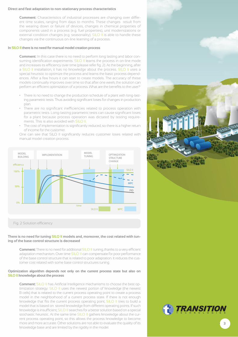
In SILO II there is no need for manual model creation process
Comment: In this case there is no need to perform long lasting and labor con-suming identification experiments. SILO II learns the process in on-line mode and increases its efficiency over time (please refer fig. 2). At the beginning, after a SILO II installation, it has no knowledge about the process. SILO II uses a special heuristic to optimize the process and learns the basic process depend-ences. After a few hours it can start to create models. The accuracy of these models continually improves over time so that after one week, the solution can perform an efficient optimization of a process. What are the benefits to the user?
• There is no need to change the production schedule of a plant with long-last-ing parametric tests. Thus avoiding significant loses for changes in production plan.
• There are no significant inefficiencies related to process operation with parametric tests. Long-lasting parametric tests can cause significant loses for a plant because process operation was dictated by testing require-ments. This is also avoided with SILO II.
• The cost of implementation is significantly reduced, so there is a higher return of income for the customer.
One can see that SILO II significantly reduces customer loses related with manual model creation process.
MODELBUILDING
MODELTUNING OPTIMIZATION
STRUCTURECHANGE
IMPLEMENTATION
e�ciency
100%
50%
0%time
SILO II
MPC
PID
MPCSILO II
Fig. 2 Solution efficiency
There is no need for tuning SILO II models and, moreover, the cost related with tun-ing of the base control structure is decreased
Comment: There is no need for additional SILO II tuning, thanks to a very efficient adaptation mechanism. Over time SILO II can compensate for poor performance of the base control structure that is related to poor adaptation. It reduces the cus-tomer cost related with some base control structures tuning.
Optimization algorithm depends not only on the current process state but also on SILO II knowledge about the process
Comment: SILO II has Artificial Intelligence mechanisms to choose the best op-timization strategy. SILO II uses the newest portion of knowledge (the newest B cells) that is related to the current process operating point to create a process model in the neighborhood of a current process state. If there is not enough knowledge that fits the current process operating point, SILO II tries to build a model that is based on stored knowledge from different operating points. If such knowledge is insufficient, SILO II searches for a better solution based on a special stochastic heuristic. At the same time SILO II gathers knowledge about the cur-rent process operating point, so this allows the process knowledge to become more and more accurate. Other solutions are not able to evaluate the quality of its knowledge base and are limited by the rigidity in the model.
• 3
Fleet optimization solution
Comment: SILO II is dedicated for different types of large-scale plants. In case of combustion process optimization, it can handle all types of energetic boilers, different fuels and different load pro-files. SILO II reaches highest performance during steady-state control, however there is a special dedicated mechanism that is activated during a transition state. Thanks to this mechanism, SILO II is able to handle operating point transi-tions (e.g. load changes). The SILO II optimizer is very easy to install and maintain. It has an effi-cient adaptation mechanism and a flexible struc-ture of the optimization task, thus it can follow changes of process characteristics and modifica-tions of production strategy. All these features make SILO II a perfect solution for a fleet optimi-zation approach.
Possibility of expert knowledge implementation
Comment: There is a possibility to implement an expert knowledge about the process, even if such knowledge is fuzzy. Users can define con-straints for chosen gains of an automatically cre-ated plant model.
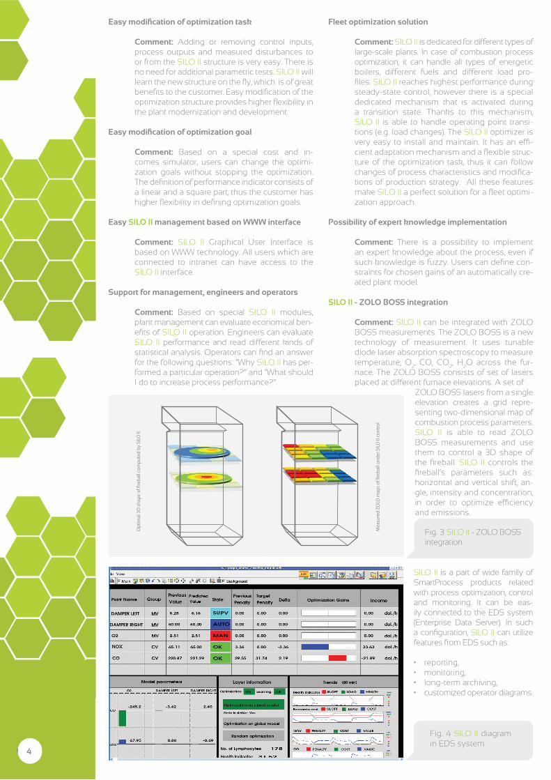
SILO II - ZOLO BOSS integration
Comment: SILO II can be integrated with ZOLO BOSS measurements. The ZOLO BOSS is a new technology of measurement. It uses tunable diode laser absorption spectroscopy to measure temperature, O
2, CO, CO
2, H
2O across the fur-
nace. The ZOLO BOSS consists of set of lasers placed at different furnace elevations. A set of
ZOLO BOSS lasers from a single elevation creates a grid repre-senting two-dimensional map of combustion process parameters.SILO II is able to read ZOLO BOSS measurements and use them to control a 3D shape of the fireball. SILO II controls the fireball’s parameters such as: horizontal and vertical shift, an-gle, intensity and concentration, in order to optimize efficiency and emissions.
• 3
Opt
imal
3D
shap
e of
�re
ball
com
pute
d by
SIL
O II
Mea
sure
d ZO
LO m
aps o
f �re
ball
unde
r SIL
O II
con
trol
SILO II is a part of wide family of SmartProcess products related with process optimization, control and monitoring. It can be eas-ily connected to the EDS system (Enterprise Data Server). In such a configuration, SILO II can utilize features from EDS such as:
• reporting,• monitoring,• long-term archiving,• customized operator diagrams.
• 4
Easymodificationofoptimizationtask
Comment: Adding or removing control inputs, process outputs and measured disturbances to or from the SILO II structure is very easy. There is no need for additional parametric tests. SILO II will learn the new structure on the fly, which is of great benefits to the customer. Easy modification of the optimization structure provides higher flexibility in the plant modernization and development.
Easymodificationofoptimizationgoal
Comment: Based on a special cost and in-comes simulator, users can change the optimi-zation goals without stopping the optimization. The definition of performance indicator consists of a linear and a square part, thus the customer has higher flexibility in defining optimization goals.
Easy SILO II management based on WWW interface
Comment: SILO II Graphical User Interface is based on WWW technology. All users which are connected to intranet can have access to the SILO II interface.
Support for management, engineers and operators
Comment: Based on special SILO II modules, plant management can evaluate economical ben-efits of SILO II operation. Engineers can evaluate SILO II performance and read different kinds of statistical analysis. Operators can find an answer for the following questions: “Why SILO II has per-formed a particular operation?” and “What should I do to increase process performance?”.
Fig. 4 SILO II diagram in EDS system
Fig. 3 SILO II - ZOLO BOSS integration
• 5
SILO II – how does it
work?
SILO II OPERATOR
SILO SUPERVISORY
SILO SUPERVISORY
m cm t m d
m f
YES
YES
PID PID
NO
NO
SUBPROCESS SUBPROCESS
m p1 m p
2
m t2
m c1
d3
d 1
m c2
y
d
d
y1
y3
PLAN
TBA
SE C
ON
TRO
LAD
VAN
CED
CO
NTR
OL
OPTIMIZED MIMO PROCESS
The optimization of power boilers is an important topic in research and in the im-plementation of projects in the power industry. The combustion process in a power boiler is a complex process, with a large number of control variables, disturbances and outputs. This is a dynamic non-linear process characterized by long response time caused by process inertia and transport delay. It is hard to control such a pro-cess using only standard SISO (Single Input Single Output) control algorithms.
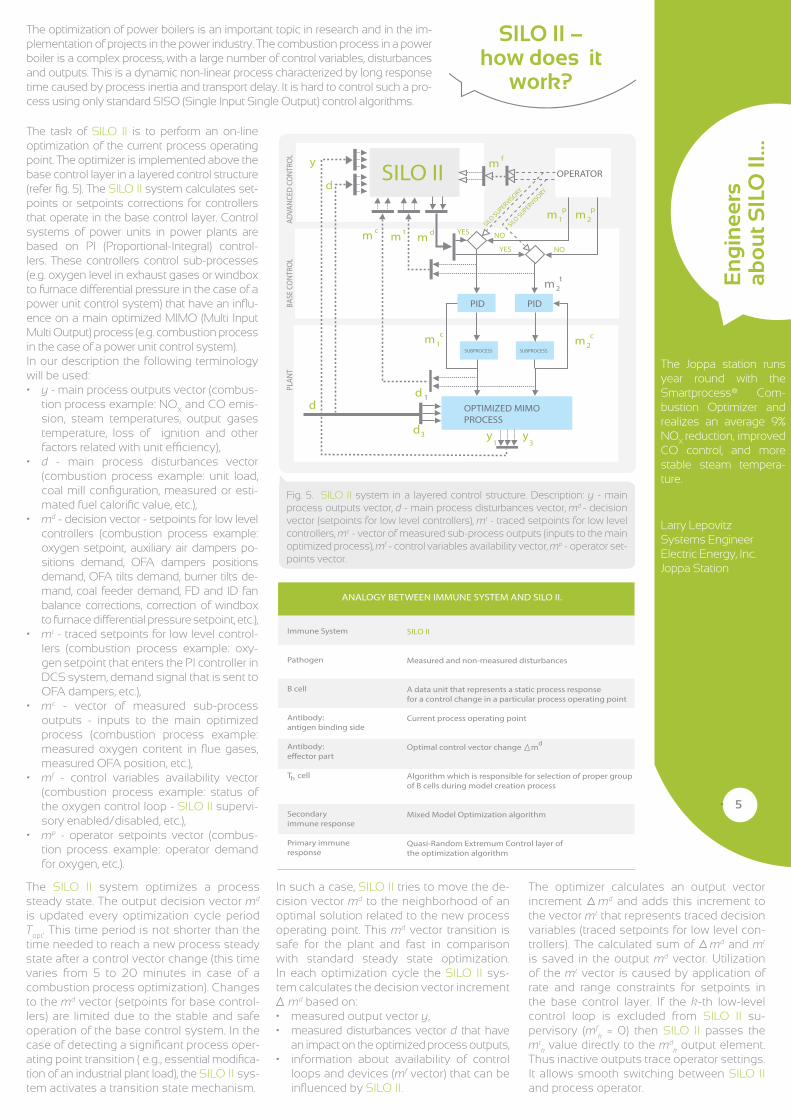
Fig. 5. SILO II system in a layered control structure. Description: y - main process outputs vector, d - main process disturbances vector, md - decision vector (setpoints for low level controllers), mt - traced setpoints for low level controllers, mc - vector of measured sub-process outputs (inputs to the main optimized process), mf - control variables availability vector, mp - operator set-points vector.
The task of SILO II is to perform an on-line optimization of the current process operating point. The optimizer is implemented above the base control layer in a layered control structure (refer fig. 5). The SILO II system calculates set-points or setpoints corrections for controllers that operate in the base control layer. Control systems of power units in power plants are based on PI (Proportional-Integral) control-lers. These controllers control sub-processes (e.g. oxygen level in exhaust gases or windbox to furnace differential pressure in the case of a power unit control system) that have an influ-ence on a main optimized MIMO (Multi Input Multi Output) process (e.g. combustion process in the case of a power unit control system).In our description the following terminology will be used:• y- main process outputs vector (combus-
tion process example: NOX and CO emis-
sion, steam temperatures, output gases temperature, loss of ignition and other factors related with unit efficiency),
• d - main process disturbances vector (combustion process example: unit load, coal mill configuration, measured or esti-mated fuel calorific value, etc.),
• md - decision vector - setpoints for low level controllers (combustion process example: oxygen setpoint, auxiliary air dampers po-sitions demand, OFA dampers positions demand, OFA tilts demand, burner tilts de-mand, coal feeder demand, FD and ID fan balance corrections, correction of windbox to furnace differential pressure setpoint, etc.),
• mt - traced setpoints for low level control-lers (combustion process example: oxy-gen setpoint that enters the PI controller in DCS system, demand signal that is sent to OFA dampers, etc.),
• mc - vector of measured sub-process outputs - inputs to the main optimized process (combustion process example: measured oxygen content in flue gases, measured OFA position, etc.),
• mf - control variables availability vector (combustion process example: status of the oxygen control loop - SILO II supervi-sory enabled/disabled, etc.),
• mp - operator setpoints vector (combus-tion process example: operator demand for oxygen, etc.).
Immune System
Pathogen
B cell
Antibody:antigen binding side
Antibody: e�ector part
T cell
Secondaryimmune response
Primary immune response
d
h
ANALOGY BETWEEN IMMUNE SYSTEM AND SILO II.
SILO II
Measured and non-measured disturbances
A data unit that represents a static process response for a control change in a particular process operating point
Current process operating point
Optimal control vector change m
Algorithm which is responsible for selection of proper group of B cells during model creation process
Mixed Model Optimization algorithm
Quasi-Random Extremum Control layer of the optimization algorithm
The SILO II system optimizes a process steady state. The output decision vector md is updated every optimization cycle period T
opt. This time period is not shorter than the
time needed to reach a new process steady state after a control vector change (this time varies from 5 to 20 minutes in case of a combustion process optimization). Changes to the md vector (setpoints for base control-lers) are limited due to the stable and safe operation of the base control system. In the case of detecting a significant process oper-ating point transition ( e.g., essential modifica-tion of an industrial plant load), the SILO II sys-tem activates a transition state mechanism.
In such a case, SILO II tries to move the de-cision vector md to the neighborhood of an optimal solution related to the new process operating point. This md vector transition is safe for the plant and fast in comparison with standard steady state optimization. In each optimization cycle the SILO II sys-tem calculates the decision vector increment
md based on:• measured output vector y,• measured disturbances vector d that have
an impact on the optimized process outputs,• information about availability of control
loops and devices (mf vector) that can be influenced by SILO II.
The optimizer calculates an output vector increment md and adds this increment to the vector mt that represents traced decision variables (traced setpoints for low level con-trollers). The calculated sum of md and mtis saved in the output md vector. Utilization of the mt vector is caused by application of rate and range constraints for setpoints in the base control layer. If the k-th low-level control loop is excluded from SILO II su-pervisory (mf
k = 0) then SILO II passes the
mtk value directly to the md
koutput element.
Thus inactive outputs trace operator settings. It allows smooth switching between SILO II and process operator.
The Joppa station runs year round with the Smartprocess® Com-bustion Optimizer and realizes an average 9% NO
X reduction, improved
CO control, and more stable steam tempera-ture.
Larry LepovitzSystems EngineerElectric Energy, Inc.Joppa Station
En
gin
eers
ab
ou
t SIL
O II
...
• 6
The SILO II operation and optimizer structure are inspired by immune system – biological structures and processes within an organism. Analogy between immune system and SILO II table (page 5) in order to provide information concerning bio-logical inspiration of our system. In SILO II system there are two main, independent modules: the Optimization and the Knowledge Gathering module. The optimization module uses the collected knowledge to find such control vector change ( md) that minimizes the follow-ing performance indicator:
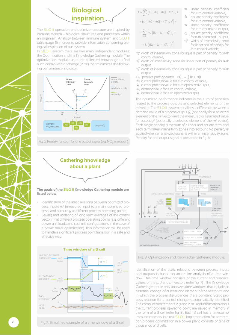
Biological inspiration
Tksy
Tkly
Linear Intensivity Zone
Square Intensivity Zone
Yk Yk ~
Setpoint
square + linear penalty
only linear penalty
no penalty
PEN
ALT
Y
Example:NO emission [mg/Nm ] 3120
180 220
200x280
Fig. 6. Penalty function for one output signal (e.g. NOX emission).
J =nm
k=1
αk |mck − mc
k | − τ lmk + +
+ βk ( |mck − mc
k | − τ smk )+2
+
+n y
k=1
γk |yk − yk | − τ lyk ++
+ δk ( |yk − yk | − τ syk )+2
linear penalty coefficien for k-th control variable,square penalty coefficient for k-th control variable,linear penalty coefficient for k-th optimized output,square penalty coefficient for k-th optimized output,width of insensitivity zone for linear part of penalty for k-th control variable,
The optimized performance indicator is the sum of penalties related to the process outputs and selected elements of the mc vector. The SILO II system penalizes a difference between a demand value of a process output y
k (optionally for a selected
element of the mc vector) and the measured or estimated value for output yk (optionally a selected element of the mc vector). Each single penalty is the sum of a linear and square term, and each term takes insensitivity zones into account. No penalty is applied when an analyzed signal is within an insensitivity zone. Penalty for one output signal is presented in fig. 6.
+ +
++
width of insensitivity zone for square part of penalty for k-th control variable,width of insensitivity zone for linear part of penalty for k-th output,width of insensitivity zone for square part of penalty for k-th output,“positive part” operator current process value for k-th control variable,current process value for k-th optimized output,demand value for k-th control variable,demand value for k-th optimized output.
Gathering knowledgeabout a plant
Identification of the static relations between process inputs and outputs is based on an on-line analysis of a time win-dow. This time window consists of the current and historical values of the y, d and mc vectors (refer fig. 7) . The Knowledge Gathering module only analyzes time windows that include an essential change of at least one element of the vector mc and in which the process disturbances d are constant. Static pro-cess reaction for a control change is automatically identified. The computed increments y and mc, and information about the current process operating point, are saved in memory in the form of a B cell (refer fig. 8). Each B cell has a timestamp. Immune memory in a real SILO II implementation for combus-tion process optimization in a power plant, consists of tens of thousands of B cells.
The goals of the SILO II Knowledge Gathering module arelisted below:
• Identification of the static relations between optimized pro-cess inputs mc (measured input to a main, optimized pro-cess) and outputs y at different process operating points;
• Saving and updating of long term averages of the control vector mc at different process operating points (e.g. different power unit loads and coal mill configurations in the case of a power boiler optimization). This information will be used to handle a significant process point transition in a safe and effective way.
oxygen setpointcorrection
OFA damperposition
NOemission
unit load
Time window of a B cell
mc1
mc2
before
beforem
c1
mc1
after
mc2
mc2
after
before
y1
after
y1
y1
d1
x
Fig.7. Simplified example of a time window of a B cell
TIMESTAMP
KNOWLEDGEGATHERINGMODULE
LONG TERMAVERAGES
IDENTIFICATIONOF STATIC PROCESSREACTION
B CELLAUTOMATICALLY IDENTIFIED TARGET
TAR
GE
TS
BA
SE
B C
ELL
SB
AS
E
USER DEFINEDTARGETS
LONG TERMMEMORY
THE NEWESTGLOBAL CELLS
STEADY-STATE
TARGETSELECTION
TRANSITION STATE LAYER
MIXED MODEL LAYER
GLOBAL MODEL LAYER
QUASI RANDOM EXTREMUM CONTROL
AUTOMATICSUB-ALGORITHM
SELECTION
SIGNIFICANT PROCESS
POINT TRANSITIO
N
OPTIMIZATION MODULE
y
y
d
d
mc
md
mt mf
Fig. 8. Optimization and Knowledge Gathering module.
Optimization module: Quasi Random
Extremum Control
αk
γk
δk
τ lmk
τ smk
τ lyk
τ syk
( ·)+ (x )+ = 12 (x + |x |)
mck
ykmc
k
yk
βk

The information stored in B cells is utilized in the model creation process which is automatically performed in each optimization cycle. The second goal of the Knowledge Gathering mo- dule is the saving and updating of long term aver-ages of the mc, d and y vectors at different process operating points. These long term averages are trans-formed into AIT (Automatically Identified Targets) objects that are used in the TransitionState layer (a sub-algorithm of the Optimization module). Each AIT has a timestamp. When a process transition state is detected, the system searches for the most recent AIT that fits the current or estimated process operating point.
∆M L =
∆mc1,1 ∆mc
1,2 . . . ∆mc1,nm
∆mc2,1 ∆mc
2,2 . . . ∆mc2,nm
......
. . ....
∆mcl,1 ∆mc
l,2 . . . ∆mcl,nm
,
• 7
Optimization module: Quasi Random
Extremum Control
In the initial phase of SILO II operation the size of the immune memory is relatively small. In analogy to the immune system one can say that the body is often attacked by new, unknown pathogens. Early on, SILO II does not have sufficient knowledge to create a mathemati-cal model of the process and solve the optimization task based on this model. A special heuristic that is applied in the QuasiRandomExtremumControl layer covers the following goals:• Gathering knowledge about the process. This is done
by modifying the md vector in such way that each modification can be treated as a standard identifica-tion experiment. New B cells are created based on these identification experiments;
• Decreasing the value of an optimized quality indicator at a long time horizon with the assumption that process distur-bances are constant at a long time horizon. In analogy to the immune system one can say that a goal of the QuasiRandomExtremumControl layer is the elimination of the pathogen at the long time horizon with the assumption that the body is attacked by one sort of pathogen at the long time horizon (a primary immune response);
• Maintaining the good conditioning of the model identifica-tion task.
A special heuristic applied in the QuasiRandomExtrem-umControl layer changes only one element of the md vector in each optimization cycle (e.g., only the oxygen setpoint is changed in case of a combustion process). In reaction to this change, the process outputs y reach a new steady state. The Knowledge Gathering module au-tomatically identifies such a static process reaction and creates a B cell. In a new optimization cycle a different element of md (e.g. OFA damper position demand) is modified and a new B cell is created. After a defined number of cycles, the best md vector value is restored and applied. This value of the md vector is related to the lowest registered value of an optimized quality indicator.The Quasi Random Extremum Control layer is executed if:• There are not enough B cells in the immune memory to
create a mathematical model of the process; • The knowledge stored in the immune memory is not
sufficient to improve the value of the performance indi-cator. It means that the model is not accurate enough. The applied increment of the mdvector calculated in the MixedModelOptimization, or the GlobalModelOptimi-zation layer (refer fig. 8), is not able to decrease the value of the quality indicator.
Steady state model based optimization is performed in the MixedModelOptimization or the GlobalModelOptimizationlayer (refer fig. 8). In both layers a model is formulated in thefollowing way:
Optimization module: Steady State
Optimalization
In the case of mixed model based optimization, elements of the matrix K (process gains) are estimated based on in-formation stored in the local observation matrices M
L and
YL, as well as the global observation matrices M
G and
YG
, where
∆y = ∆mdK
mink
{ kT η∆MTL ∆ML + ∆MT
G ∆MG k
− 2kT η∆MTL ∆yL + ∆MT
G ∆yG }
v
v
with constraints
Each of the l rows of the ML matrix consist of in-
crements mci of elements of the mc vector. These
increments are stored in a local B cell. This local B cell belongs to the set of l youngest local B cells. The local B cell is a selected B cell that is related to the cur-rent process operating point. Such a B cell was created when a historical process operating point (e.g. unit load in case of a combustion process optimization in a power boiler) was similar to the current process operating point. By analogy, the matrix M
G consists
of mc vector increments that are stored in the set of g youngest global B cells. Global B cell selection is based only on a time criterion. Each of the l rows of the Y
L matrix consist of y vector element incre-
ments yi that are stored in a local B cell. By analogy,
the matrix YG consists of y vector increments that
are stored in the set g youngest global B cells. A vector k is related to a selected column of the pro-cess gains matrix K. It represents gains between pro-cess inputs and selected process output. In the case of a MISO (Multi Input Single Output) model, a spe-cial additional optimization task is executed in order to estimate a vector k value
∆Y L =
∆y1,1 ∆y1,2 . . . ∆y1,ny∆y2,1 ∆y2,2 . . . ∆y2,ny...
.... . .
...∆yl,1 ∆yl,2 . . . ∆yl,ny
.
k l ≤ k ≤ ku

The computed increment md is added to the current value of the mt vector. This sum is saved as the optimizer output md.
The increment of inactive elements of the md vector (defined by the mf vector – refer fig. 5) is set to zero. The Mixed Model Optimization layer is activated when SILO II has sufficient knowledge about static process dependencies in the close neighborhood of the current process operating point. If there are not enough local B cells in memory, then only global B cells will be used to create a global model. However if there are not enough global B cells in memory (initial phase of SILO II operation), or further improvement of a performance indicator value is not possible based on the model, then SILO II switches to the QuasiRandomExtremumControl layer. By analogy to the immune system, the operation of the MixedModelOptimizationlayer can be compared to a secondary immune response. The SILO II system uses the knowledge stored in the B cells to provide the fast and effective elimination of pathogens (process disturbances compensation).
md = mt + ∆md
Optimization module: Transition of Process
Operating Point
The newest version of SILO II has a new algorithm that is able to handle a signif-icant process transition in an effective way. This algorithm is implemented in the Transition State layer in the Opti-mization module of SILO II (refer fig. 8). In the case of a combustion process optimization, this new mechanism al-lows for optimization of relatively small power units characterized by frequent transitions of unit load.
The AIT (Automatically Identified Tar-gets) and UDT (User Defined Targets) are used to move the control vector val-ue to a point that lies in a close neigh-borhood of an optimal solution related with the new process operating point. This transition is fast. A new process operating point is a starting point for model based optimization.
min∆m d
nm
k=1
αk mck + ∆md − mc
k − τ lmk +
+ βk mck + ∆md − mc
k − τ smk +
2+
+n y
k=1
γk yk + ∆mdK k − yk − τ lyk +
+ δk yk + ∆mdK k − yk − τ syk +
2
with constraints
∆mdlow ≤ ∆md ≤ ∆md
hi ,
mdlow ≤ mt + ∆md ≤ md
hi
• 8
The presented additional optimization task, allows for the utilization of constraints related with automatically identified model gains. In most SILO II implementations these gains are unbounded. In such a case, a Least Square Method can be used to estimate elements of the gain matrix K. Thanks to the additional optimization task, the system can use someexpert knowledge about the range of gain values for selected dependences between process inputs and outputs. An optimal increment md of the md vector is computed based on the identified model. This increment minimizes the value of a quality indicator. It also fulfills constraints for a maximal absolute increment of the md vector in one optimization cycle. The following optimization task is solved in each optimization cycle:
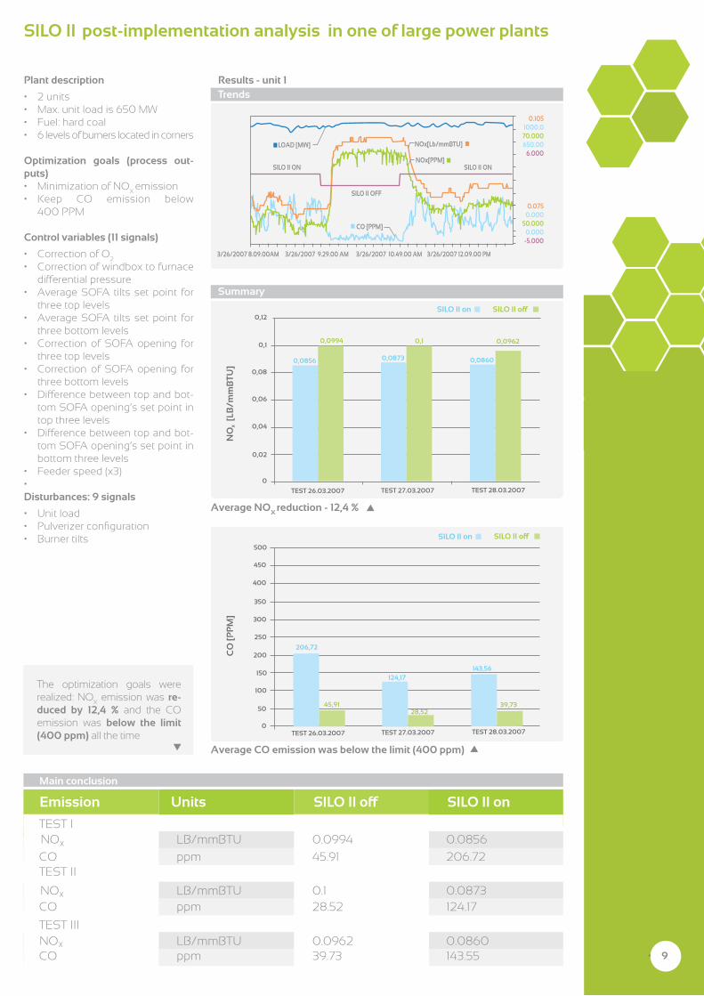
SILO II post-implementation analysis in one of large power plants
• 9
Plant description
• 2 units• Max. unit load is 650 MW• Fuel: hard coal• 6 levels of burners located in corners
Optimization goals (process out-puts)• Minimization of NO
X emission
• Keep CO emission below 400 PPM
Control variables (11 signals)
• Correction of O2
• Correction of windbox to furnace differential pressure
• Average SOFA tilts set point for three top levels
• Average SOFA tilts set point for three bottom levels
• Correction of SOFA opening for three top levels
• Correction of SOFA opening for three bottom levels
• Difference between top and bot-tom SOFA opening’s set point in top three levels
• Difference between top and bot-tom SOFA opening’s set point in bottom three levels
• Feeder speed (x3)• Disturbances: 9 signals
• Unit load• Pulverizer configuration• Burner tilts
Emission Units SILO II off SILO II on
TEST II
TEST III
TEST INO LB/mmBTU 0.0994 0.0856
CO ppm 45.91 206.72
NO LB/mmBTU 0.1 0.0873CO ppm 28.52 124.17
NO LB/mmBTU 0.0962 0.0860CO ppm 39.73 143.55
x
x
x
The optimization goals were realized: NO
X emission was re-
duced by 12,4 % and the CO emission was below the limit (400 ppm) all the time
3/26/2007 8.09.00AM 3/26/2007 9.29.00 AM 3/26/2007 10.49.00 AM 3/26/2007 12.09.00 PM
0.1051000.0
70.000650.00
6.000
0.0750.000
50.0000.000-5.000
NOx[Lb/mmBTU]
NOx[PPM]SILO II ONSILO II ON
LOAD [MW]
CO [PPM]
SILO II OFF
Trends
Summary
0,0994 0,1
0,0856 0,0873 0,0860
0,0962
TEST 26.03.2007 TEST 27.03.2007 TEST 28.03.2007
0,12
0,1
0,08
0,06
0,04
0,02
0
SILO II on SILO II off
NO
[L
B/m
mB
TU]
x
Average NOX
reduction - 12,4 %
45,9128,52
206,72
124,17143,56
CO
[PP
M]
TEST 26.03.2007 TEST 27.03.2007 TEST 28.03.2007
SILO II on SILO II off
39,73
500
450
400
350
300
250
200
150
100
50
0
Average CO emission was below the limit (400 ppm)
Main conclusion
Results - unit 1
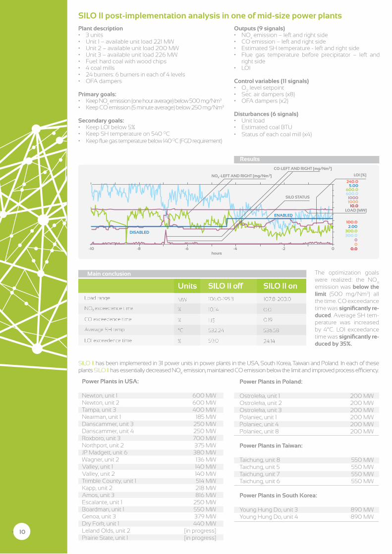
Power Plants in USA:
Newton, unit 1 600 MWNewton, unit 2 600 MWTampa, unit 3 400 MWNearman, unit 1 185 MWDanscammer, unit 3 250 MWDanscammer, unit 4 250 MWRoxboro, unit 3 700 MWNorthport, unit 2 375 MWJP Madgett, unit 6 380 MWWagner, unit 2 136 MWValley, unit 1 140 MWValley, unit 2 140 MWTrimble County, unit 1 514 MWKapp, unit 2 218 MWAmos, unit 3 816 MWEscalante, unit 1 250 MWBoardman, unit 1 550 MWGenoa, unit 3 379 MWDry Fork, unit 1 440 MWLeland Olds, unit 2 [in progress]Prairie State, unit 1 [in progress]
240.05.00
600.0600.0
10001000
10.0
100.02.00
300.0300.0
00
0.0
LOAD [MW]
LOI [%]
CO-LEFT AND RIGHT [mg/Nm ]
NO -LEFT AND RIGHT [mg/Nm ]
SILO STATUS
ENABLED
DISABLED
hours-10 -8 -6 -4 -2 0
3
3
X
Plant description• 3 units• Unit 1 – available unit load 221 MW• Unit 2 – avail able unit load 200 MW• Unit 3 – available unit load 226 MW• Fuel: hard coal with wood chips• 4 coal mills• 24 burners: 6 burners in each of 4 levels• OFA dampers
Primary goals:• Keep NO
x emission (one hour average) below 500 mg/Nm3
• Keep CO emission (5 minute average) below 250 mg/Nm3
Secondary goals:• Keep LOI below 5%• Keep SH temperature on 540 0C• Keep flue gas temperature below 140 0C (FGD requirement)
The optimization goals were realized: the NO
X
emission was below the limit (500 mg/Nm3) all the time. CO exceedance time was significantlyre-duced. Average SH tem-perature was increased by 4°C. LOI exceedance time was significantlyre-duced by 35%.
Power Plants in Poland:
Ostroleka, unit 1 200 MWOstroleka, unit 2 200 MWOstroleka, unit 3 200 MWPolaniec, unit 1 200 MWPolaniec, unit 4 200 MWPolaniec, unit 8 200 MW
Power Plants in Taiwan:
Taichung, unit 8 550 MWTaichung, unit 5 550 MWTaichung, unit 7 550 MWTaichung, unit 6 550 MW
Power Plants in South Korea:
Young Hung Do, unit 3 890 MWYoung Hung Do, unit 4 890 MW
Outputs (9 signals)• NO
x emission – left and right side
• CO emission – left and right side• Estimated SH temperature - left and right side• Flue gas temperature before precipitator – left and
right side• LOI
Control variables (11 signals)• O
2 level setpoint
• Sec. air dampers (x8)• OFA dampers (x2)
Disturbances (6 signals)• Unit load• Estimated coal BTU• Status of each coal mill (x4)
SILO II post-implementation analysis in one of mid-size power plants
Results
SILO II has been implemented in 31 power units in power plants in the USA, South Korea, Taiwan and Poland. In each of these plants SILO II has essentially decreased NO
X emission, maintained CO emission below the limit and improved process efficiency.
Main conclusion
• 10

ScientificPublications
SILOIIsystemwasdescribedin14scientificpublications.Select-ed publications are presented below:
[1] K. Wojdan, K. Świrski, M. Warchol, G. Jarmoszewicz, T. Chomiak: „Bio-inspired process control”, book chapter “Bio-inspired com-puting and communication networks” edited by Yang Xiao, CRC Press – Taylor and Francis Group, ISBN 978-1-4200-8032-2, Boca Raton, USA, March 2011
[2] K. Wojdan, K. Świrski, M. Warchol, J. Milewski, A. Miller: “A Prac-tical Approach To Combustion Process Optimization Using an Improved Immune Optimizer”, Sustainable Research and Inno-vation Proceedings, vol. 3, Kenya, 2011
[3] K. Wojdan, K. Świrski, and M. Warchol: “Transition State Layer in the Immune Inspired Optimizer”, Trends in Applied Artificial In-telligence, Lecture Notes in Artificial Intelligence, vol. 6096, pp. 11–20, 2010
[4] K. Wojdan, K. Świrski, M. Warchoł, M. Maciorowski: “Condition-ing of Model Identification Task in Immune Inspired Optimizer SILO”, book chapter “IAENG Transactions on Engineering Tech-nologies Volume 3”, American Institute of Physics (AIP), Novem-ber 2009
Awards
SILO II is protected by patents in USA, China, India and Poland. SILO II has received the following awards:
• Silver medal at International Exhibition “Innovations, Research and New Technologies - INNOVA 2006”, Brussels, 2006
• Diploma from Polish Ministry of Science at Polish Research Exhibition, Warsaw 2007
• Product of the Year 2007 by Control Engineering magazine, Warsaw 2007
• Polish Product of the Future 2008 by Polish Agency for Enter-prise Development

Transition Technologies S.A.Pawia 55, 01-030 WarszawaTel.: +48 22 331 80 20Fax: +48 22 331 80 30E-mail: [email protected]
M.Sc. Eng. Łukasz ŚladewskiProduct ManagerM.: +48 601 805 120 F.: +48 (0) 22 [email protected]
Contact
About Transition Technologies
Since over 20 years we have been providing our customers with the highest world’s levelITsolutionsbasedonthelatesttechnologies.Ourofferincludes:
• Development and distribution of software for utility sectors• Optimization of technological processes• Electrical energy and gas trading• Risk management• Programming• Engineering services• Solutions to mobile technologies • Research and development projects• Software service outsourcing• Software consulting
• Our established technological leadership is an outcome of a long-term experience in advanced projects implementation and application of the most innovative solutions, which together have resulted in a number of competitive realizations adjusted to the customers’ needs.We believe that our employees are the key to our success. Our team consists of ex-ceptionally educated young people – graduates of major polish technical universities. Their knowledge and professional consultancy in application of delivered solutions determine the quality and innovation of our products. With offices located in five Polish cities; Warsaw, Lodz, Bialystok, Wroclaw and Ostrow Wielkopolski in Germany and in United States our company maintains rapid and dynamic growth.
Ph.D. Eng. Konrad WojdanR&D Team ManagerM.: +48 603 910 108 F.: +48 (0) 22 [email protected]


