SPECTRAL TECHNOLOGIES FOR ANALYZING 3D CONVERGING-DIVERGING NOZZLE, VENTURI TUBE, AND 90-DEGREE BEND DUCT

Undergraduate Honors Thesis

In Partial Fulfillment of the Requirements for Graduation with Distinction and Honors in the

Department of Mechanical Engineering at The Ohio State University

by

Rory C. Kennedy

Spring 2012

Advisor: Oliver G. McGee III, Ph.D. - Howard University, Washington, D.C.

This work was supported by the United Technologies Corporation and the Air Force Research Laboratory

Abstract

Computational fluid dynamics (CFD) is used to provide detailed predictions of complex

fluid flows. CFD enables scientists and engineers to perform numerical experiments or computer

simulations in a virtual flow laboratory. This study focuses on CFD for predicting the

performance map of various Turbomachinery and nozzle configurations. The performance map

can be characterized as the pressure ratio and efficiency of aircraft engines. Since small

improvements in engine efficiency can lead to huge savings in fuel costs for a fleet of

commercial aircraft, scientists and engineers are very interested in CFD tools that can give

accurate quantitative predictions of engine performance maps without the need to run as many

costly full scale wind tunnel tests. A three-dimensional (3D) spectral procedure has been

developed to predict the flow solutions for the various nozzle configurations. The flow

predictions have been charted against the evidence of well-established test data previously

obtained in the literature. A spectral analysis procedure was formulated to reduce the governing

coupled nonlinear parabolic partial differential equations to associated coupled nonlinear

algebraic equations for the unsteady viscous compressible flow inside the geometry

configurations. No conventional ordinary differential equations and associated time-marching

techniques linked with finite element, volume, or differencing methodologies were needed.

Favorable agreement is shown between the present 3D spectral method predictions and

previously published 3D finite volume predictions of the transonic flow. The phenomenology of

3D spectral calculated secondary flow in the nozzles were traced and compared to that

previously published in the literature. The favorable results obtained from the study shows clear

evidence that the 3D spectral procedure developed can be an important tool in analyzing aircraft

engines to improve performance efficiencies.

iii

Acknowledgements

This thesis is a compilation of countless hours of work I have performed for the past three

years. None of this would be possible without my advisor and mentor Professor Oliver McGee. I

met him three years ago serendipitously and I have been working with him ever since. He

brought me with him to NASA Glenn Research Center to assist him with his research during

summers 2010 and 2011, and he also brought me to Washington D.C. for a quarter to work with

him and alongside a couple of brilliant Howard University mechanical engineering students. Not

only has he given me this amazing opportunity, but he has also helped me push myself in the

classroom and in other career choices.

I would like to thank Dr. Rob Siston of Ohio State University, Dr. Scott Sawyer of Akron

University, NASA Glenn Research Center Employees Mark Celestina and Rod Chima, and

undergraduate engineering students of Howard University Rishi Jaglal and Michael Gallion for

their assistance in helping me pull this all together.

I would also like to thank the Ohio State University’s College of Engineering, Howard

University’s College of Engineering, and the Air Force Research Laboratory for funding the

project for the past three years.

Lastly, I would like to give thanks to my parents Mark and Julie Kennedy for putting up

with me for the last three years. They have given me tremendous support and without them, I

wouldn’t have been able to do this. Thank you Mom and Dad for everything.

iv

Table of Contents

1.1 Methodologies ----------------------------------------------------------------------------------------- 2 1.2 Purpose of Research ---------------------------------------------------------------------------------- 4

2.1 Converging-Diverging Nozzle ---------------------------------------------------------------------- 5 2.2 Venturi Tube ------------------------------------------------------------------------------------------ 17 2.3 Rectangular 90-Degree Bend Duct ---------------------------------------------------------------- 22

Abstract --------------------------------------------------------------------------------------------------------- ii

Acknowledgements ------------------------------------------------------------------------------------------ iii

Table of Contents --------------------------------------------------------------------------------------------- iv

List of Figures ------------------------------------------------------------------------------------------------- v

List of Tables-------------------------------------------------------------------------------------------------- vii

Chapter 1: Introduction --------------------------------------------------------------------------------------- 1

Chapter 2: Findings of Work Completed ------------------------------------------------------------------ 5

Chapter 3: Conclusion and Future Work ------------------------------------------------------------------ 29

References ----------------------------------------------------------------------------------------------------- 31

Appendix A: Converging-Diverging Nozzle ------------------------------------------------------------- 32

Appendix B: Venturi Tube Industry Nozzle -------------------------------------------------------------- 40

v

List of Figures

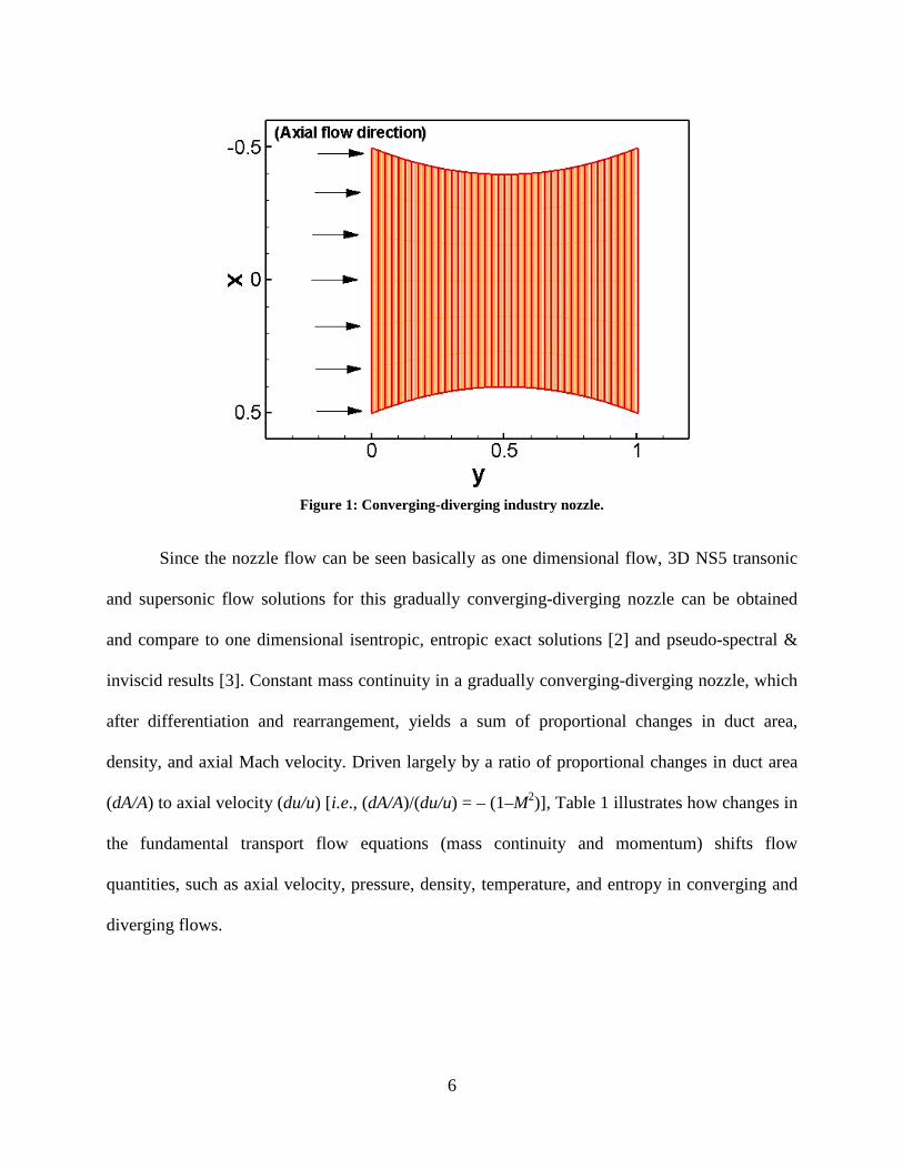
Figure 1: Converging-diverging industry nozzle.--------------------------------------------------------- 6

Figure 2: Findings of transonic and supersonic transport axial Mach flow across a gradually converging-diverging nozzle, comparing exact 1-D isentropic (shown in red), exact 1-D entropic (shown in blue) [2], 3D NS5 (shown in magenta), and 3D NS8 (shown in black)) with published findings of Hanley [3], comparing a pseudo-spectral computational transport analysis with an inviscid transport theory (right). -------------------------------------------------- 8

Figure 3: Findings of transonic and supersonic transport flow properties (axial Mach, density, temperature, and pressure) across a gradually converging-diverging nozzle, comparing exact 1-D isentropic (shown in red), exact 1-D entropic (shown in blue), 3D NS5 (shown in magenta), and 3D NS8 (shown in black). ------------------------------------------------------------ 8

Figure 4: Results of 3D NS5 steady-state conservative transonic-supersonic flow solutions computed using Legendre non-periodic spectral approximations using 220 terms for each flow state (density, fluidic velocity (u,v,w), and temperature) incorporating 40,000 points in passage. Results are normalized to the maximum non-dimensional values. -------------------- 9

Figure 5: Results of 3D NS8 steady-state conservative transonic-supersonic flow solutions computed using Legendre non-periodic spectral approximations using 220 terms for each flow state (density, fluidic velocity (u,v,w), and temperature) incorporating 40,000 points in passage. Results are normalized to the maximum non-dimensional values. ------------------- 10

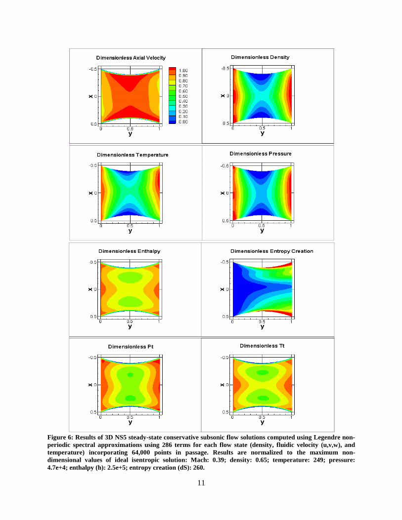
Figure 6: Results of 3D NS5 steady-state conservative subsonic flow solutions computed using Legendre non-periodic spectral approximations using 286 terms for each flow state (density, fluidic velocity (u,v,w), and temperature) incorporating 64,000 points in passage. Results are normalized to the maximum non-dimensional values of ideal isentropic solution: Mach: 0.39; density: 0.65; temperature: 249; pressure: 4.7e+4; enthalpy (h): 2.5e+5; entropy creation (dS): 260. -------------------------------------------------------------------------------------- 11

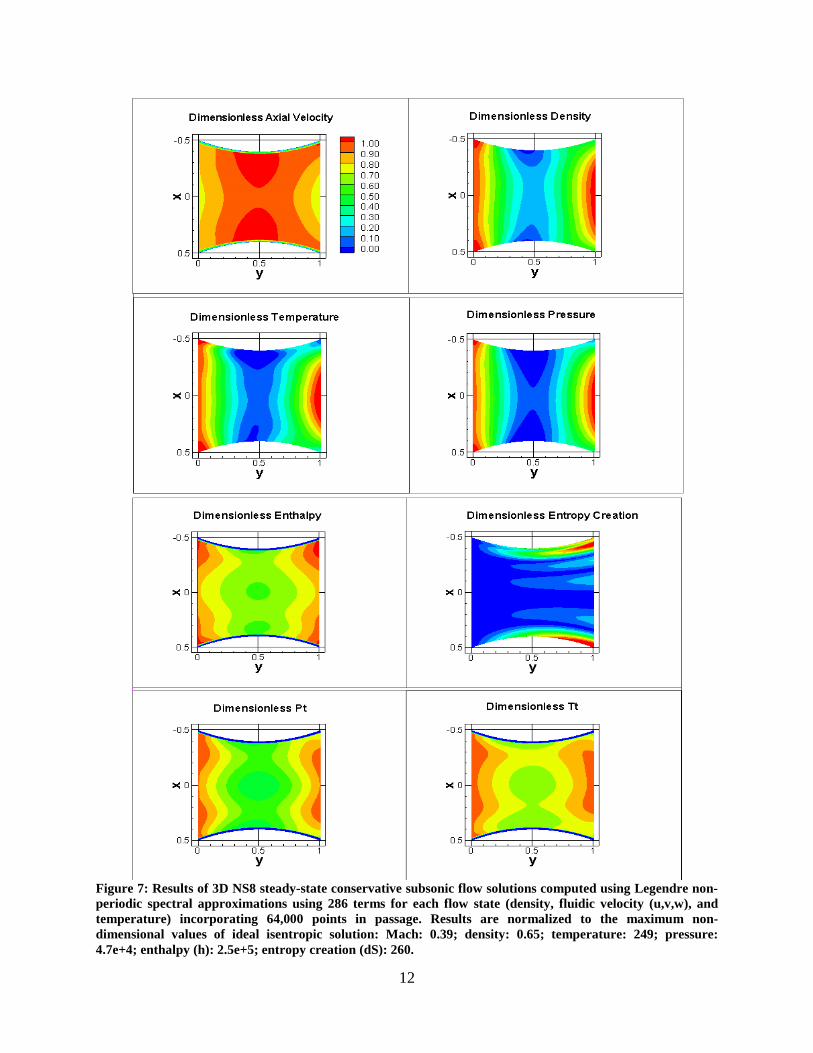
Figure 7: Results of 3D NS8 steady-state conservative subsonic flow solutions computed using Legendre non-periodic spectral approximations using 286 terms for each flow state (density, fluidic velocity (u,v,w), and temperature) incorporating 64,000 points in passage. Results are normalized to the maximum non-dimensional values of ideal isentropic solution: Mach: 0.39; density: 0.65; temperature: 249; pressure: 4.7e+4; enthalpy (h): 2.5e+5; entropy creation (dS): 260. -------------------------------------------------------------------------------------- 12

Figure 8: Computational and physical Chebyshev grids of a gradually converging-diverging nozzle for 3D NS5/NS8 analyses. Physical grid (x y z) = (40 × 40 × 40) points. ----------- 13

Figure 9: Computational grid (ξ × η × ζ) = (40 × 40 × 40) points. ----------------------------------- 13

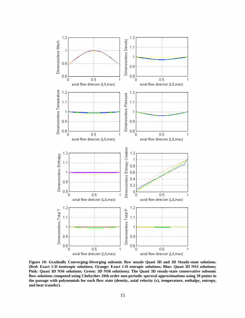
Figure 10: Gradually Converging-Diverging subsonic flow nozzle Quasi 3D and 3D Steady-state solutions. (Red: Exact 1-D isentropic solutions; Orange: Exact 1-D entropic solutions; Blue:

vi

Quasi 3D NS3 solutions; Pink: Quasi 3D NS6 solutions; Green: 3D NS8 solutions). The Quasi 3D steady-state conservative subsonic flow solutions computed using Chebyshev 20th order non-periodic spectral approximations using 20 points in the passage with polynomials for each flow state (density, axial velocity (v), temperature, enthalpy, entropy, and heat transfer). -------------------------------------------------------------------------------------- 15

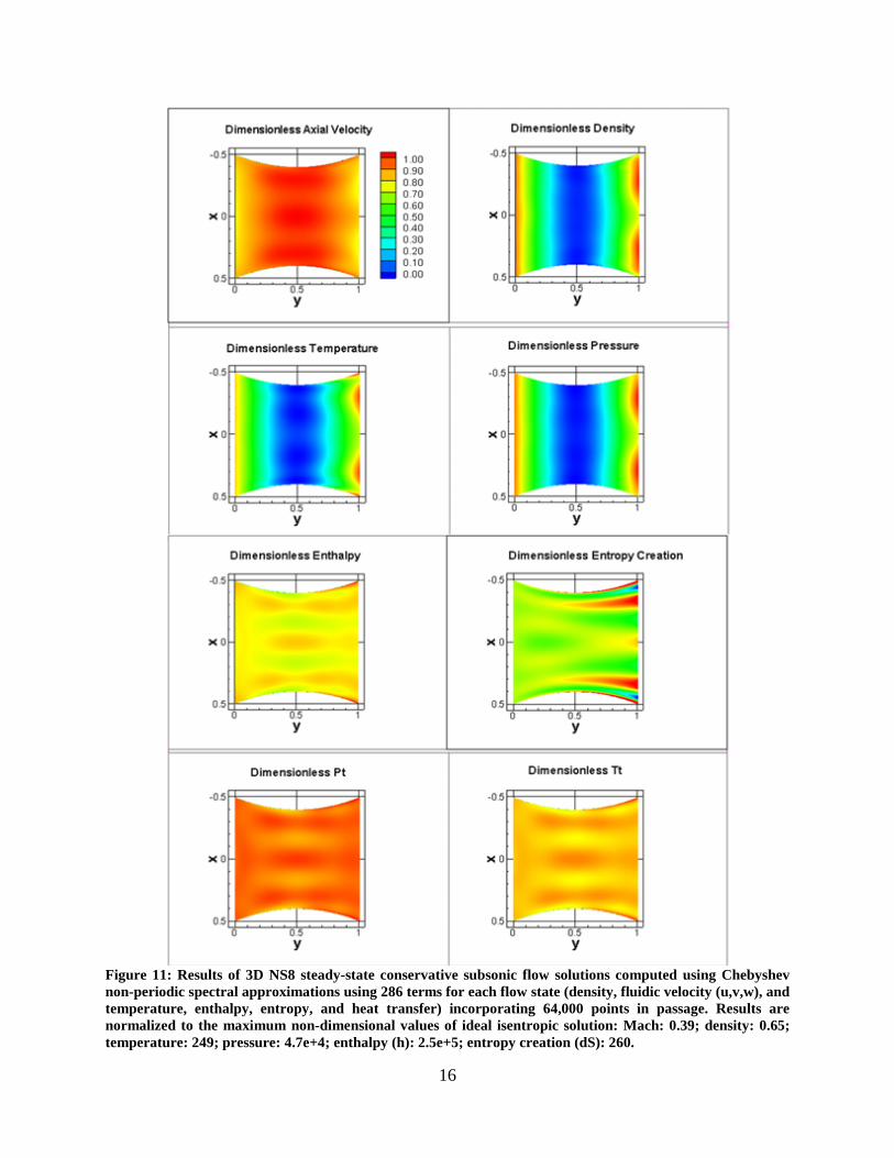
Figure 11: Results of 3D NS8 steady-state conservative subsonic flow solutions computed using Chebyshev non-periodic spectral approximations using 286 terms for each flow state (density, fluidic velocity (u,v,w), and temperature, enthalpy, entropy, and heat transfer) incorporating 64,000 points in passage. Results are normalized to the maximum non-dimensional values of ideal isentropic solution: Mach: 0.39; density: 0.65; temperature: 249; pressure: 4.7e+4; enthalpy (h): 2.5e+5; entropy creation (dS): 260. ---------------------- 16

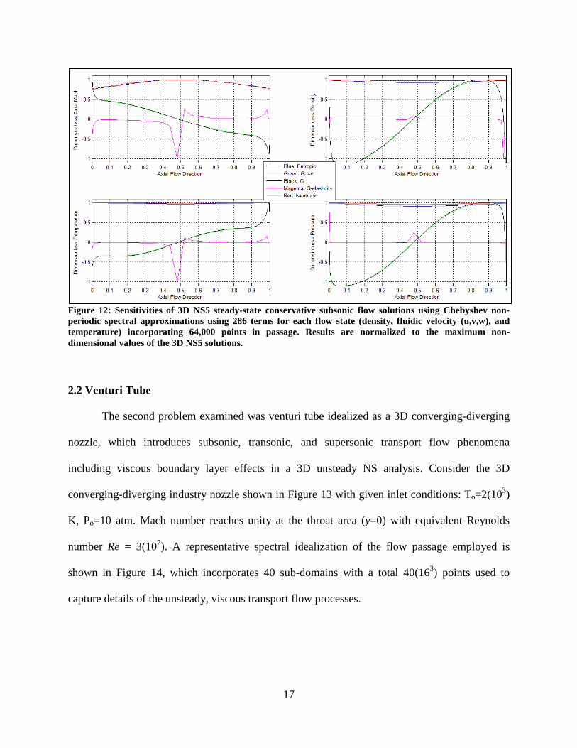
Figure 12: Sensitivities of 3D NS5 steady-state conservative subsonic flow solutions using Chebyshev non-periodic spectral approximations using 286 terms for each flow state (density, fluidic velocity (u,v,w), and temperature) incorporating 64,000 points in passage. Results are normalized to the maximum non-dimensional values of the 3D NS5 solutions. 17

Figure 13: Uniform physical grid (Legendre non-periodic computational approximation) of the 3D venturi tube industry nozzle. --------------------------------------------------------------------- 18

Figure 14: Uniform physical grid (Legendre non-periodic computational approximation) of the 3D venturi tube industry nozzle with 40 sub-domains denoted by color. Each sub-domain has 4,096 points (16x16x16 xyz) for a total of 163,840 points through the nozzle passage 18

Figure 15: Steady state findings of transonic and supersonic transport flow properties (axial Mach, density, temperature, and pressure) across a gradually converging-diverging industry nozzle, comparing exact 1D isentropic (shown in red), exact 1D entropic (shown in blue), 3D NS5 Legendre non-periodic spectral calculation (shown in magenta), and 3D NS8 Legendre non-periodic spectral calculation (shown in black) solutions. ----------------------- 20

Figure 16: Results of 3D NS8 steady-state conservative transonic and supersonic flow solutions computed along with the sensitivities using Legendre non-periodic spectral approximations using 192 terms for each flow state (density, fluidic velocity (u,v,w), and temperature, 960 total terms) incorporating 163,840 points in passage. Results are normalized to the maximum non-dimensional values of the 3D NS8 solutions; the 3D NS8 loss sensitivity measures for the run was also examined, and are normalized to the maximum non-dimensional values of the G-stress and G-entropy. ----------------------------------------------- 21

Figure 17: Joy’s [4] 90 degree rectangular cross sectional bend with a 15 in. radius experimental configuration. ------------------------------------------------------------------------------------------- 22

Figure 18: Joy’s [4] velocity profiles measured at each marked station. ----------------------------- 23

Figure 19: 90 degree square cross sectional bend created to analyze with the spectral methods. 24

vii

Figure 20: Axial velocity cross sectional contours of the 90 degree square cross sectional bend showing the formation of a separation bubble and the existence of secondary circulation development. -------------------------------------------------------------------------------------------- 25

Figure 21: Comparison of pressure loss versus Reynolds curvature effect of experimental results of White’s [5], Collins and Dennis [6], and Dean’s [7] empirical equations for laminar fully developed curved flow. -------------------------------------------------------------------------------- 27

Figure 22: Comparison of scaled pressure loss versus scaled Reynolds curvature effects of experimental results of Ito’s [9] [8] empirical equations for turbulent flow in rectangular bends. ---------------------------------------------------------------------------------------------------- 28

List of Tables

Table 1: Subsonic and supersonic flows in converging and diverging nozzles.---------------------- 7

Table 2: Dependent variables sensitivities used during analyses. ------------------------------------- 14

1

Chapter 1: Introduction

The goal of computational fluid dynamics (CFD) is to provide detailed predictions of

complex fluid flows of all sorts. CFD enables scientists and engineers to perform numerical

experiments or computer simulations in a virtual flow laboratory reducing costly full-scale tests.

This thesis focuses on CFD for predicting the performance map of various nozzle and geometry

configurations. The performance map can be characterized as the pressure ratio and efficiency of

aircraft engines. Since small improvements in engine efficiency can lead to huge savings in fuel

costs for a fleet of commercial aircraft, scientists and engineers are very interested in CFD tools

that can give accurate quantitative predictions of engine performance maps [1]. In the early

literature only qualitative comparisons were made against experimental Mach contours.

There are many reasons why performance predictions in the early literature were scarce.

One reason is in the past, computers could not effectively calculate the efficiency and loss due to

its high dependence on viscous effects, which requires high grid resolution for successful

calculation [1]. Currently, computers that are capable of performing such calculations are widely

available for CFD analysts. Another reason for the scarcity of performance predictions in the

early literature is it was difficult to obtain experimental data due to the small components and

high speeds needed for transonic turbomachinery tests. Now with advance measuring

technologies and high speed wind tunnels available to scientists, accurate test data of various

transonic systems is obtainable. The data is used to validate CFD methods in virtual laboratories.

CFD predictions are now becoming widely available and provide useful information for

scientists and engineers to help them develop and test full scale turbomachinery prototypes.

2

1.1 Methodologies

A three-dimensional spectral procedure (reduced ordered method (ROM) analysis) has

been developed to predict the Navier-Stokes flow solutions of various transport systems.

Specifically, the transport systems are modeled as a hydrodynamic continuum utilizing only

nodal data to describe the arbitrary volume in which the 3D unsteady Navier-Stokes equations

(Equations 1-5) were explicitly solved. A spectral analysis procedure was formulated to reduce

the governing coupled nonlinear parabolic partial differential equations to associated coupled

nonlinear algebraic equations for the unsteady viscous compressible flow. To achieve this, the

flow was subjected to constraints imposed by an assumed hydrodynamic state field (i.e., density,

axial, swirl, radial velocities, temperature, enthalpy, entropy, and conducted-heat) at each fluidic

point comprised of mathematically complete, orthonormal polynomials in coupled space-time

multiplied by generalized coefficients. The coefficients were determined by constraining the

polynomial series to satisfy the governing partial differential equations, initial conditions, and

boundary conditions of the transonic flow inside the transport systems. No conventional ordinary

differential equations and associated time-marching techniques linked with finite element,

volume or differencing methodologies were needed.

For solving the nonlinear 3D convection-diffusion problems of high Reynolds number,

the ROM analysis is implemented on variable geometry configurations through sub-domain

isoparametric mapping and generalized Fourier series approximation theory. The 3D Navier-

Stokes equation system (NS5) solved, including continuity, three directional (radial, axial,

tangential) momentum, and energy involving five (5) unknown fluidic properties (density, radial,

axial, and tangential velocities, and temperature), are:

3

Continuity

0)()()()(

=+++dz

wddy

vddx

uddt

d ρρρρ (1)

Radial (x) Momentum

𝜌 𝑑(𝑢)

𝑑𝑡+ 𝜌𝑢 𝑑(𝑢)

𝑑𝑥+ 𝜌𝑣 𝑑(𝑢)

𝑑𝑦+ 𝜌𝑤 𝑑(𝑢)

𝑑𝑧+ 𝑑𝑃

𝑑𝑥− 𝜇 �𝑑

2(𝑢)𝑑𝑥2

+ 𝑑2(𝑢)𝑑𝑦2

+ 𝑑2(𝑢)𝑑𝑧2

� = 0 (2)

Axial (y) Momentum

𝜌 𝑑(𝑣)𝑑𝑡

+ 𝜌𝑢 𝑑(𝑣)𝑑𝑥

+ 𝜌𝑣 𝑑(𝑣)𝑑𝑦

+ 𝜌𝑤 𝑑(𝑣)𝑑𝑧

+ 𝑑𝑃𝑑𝑦− 𝜇 �𝑑

2(𝑣)𝑑𝑥2

+ 𝑑2(𝑣)𝑑𝑦2

+ 𝑑2(𝑣)𝑑𝑧2

� = 0 (3)

Tangential (z) Momentum

𝜌 𝑑(𝑤)

𝑑𝑡+ 𝜌𝑢 𝑑(𝑤)

𝑑𝑥+ 𝜌𝑣 𝑑(𝑤)

𝑑𝑦+ 𝜌𝑤 𝑑(𝑤)

𝑑𝑧+ 𝑑𝑃

𝑑𝑧− 𝜇 �𝑑

2(𝑤)𝑑𝑥2

+ 𝑑2(𝑤)𝑑𝑦2

+ 𝑑2(𝑤)𝑑𝑧2

� = 0 (4)

3D Energy

𝜌 𝑑(𝐶𝑣𝑇)𝑑𝑡

+ 𝜌𝑢 𝑑(𝐶𝑣𝑇)𝑑𝑥

+ 𝜌𝑣 𝑑(𝐶𝑣𝑇)𝑑𝑦

+ 𝜌𝑤 𝑑(𝐶𝑣𝑇)𝑑𝑧

+ 𝑃∇𝑈 − 𝜅 �𝑑2(𝑇)𝑑𝑥2

+ 𝑑2(𝑇)𝑑𝑦2

+ 𝑑2(𝑇)𝑑𝑧2

� − Φ = 0 (5) The pressure can be calculated from the equation of state:

RTP ρ= (6)

The flow systems were subject to non-slip velocity conditions on all surfaces.

The 3D Navier-Stokes equation system (NS7) solved, includes the NS5 system with the

energy equation substituted by two additional equations of enthalpy (h, internal energy plus

thermal energy, dh, work), and entropy creation (ds, losses), plus an additional equation for heat

conductivity involving eight (8) unknown fluidic properties (density, radial, axial, and tangential

velocities, temperature, enthalpy (h, internal energy plus thermal energy, dh, work), entropy

creation (ds), and added heat (dQ, effecting temperature distribution through heat conductivity):

4

Enthalpy

𝜌 𝑑(ℎ)𝑑𝑡

+ 𝜌𝑢 𝑑(ℎ)𝑑𝑥

+ 𝜌𝑣 𝑑(ℎ)𝑑𝑦

+ 𝜌𝑤 𝑑(ℎ)𝑑𝑧

− 𝑑𝑃𝑑𝑡− 𝜅∇2𝑇 − Θ − 𝜇(𝑢∇2𝑢 + 𝑣∇2𝑣 + 𝑤∇2𝑤) = 0 (7)

Entropy Creation

0)( 2

2

2

2

2

2

=Θ−++−dz

Tddy

Tddx

TdTds κ (8)

Heat Conductivity

0)( 2

2

2

2

2

2

=+++dz

Tddy

Tddx

TddQ κ (9)

1.2 Purpose of Research

If reduced-ordered spectral technologies can be proved to find smooth, unique, and

computationally exact solutions to 3D unsteady NS transport systems, CFD methodologies

would be change forever. It would allow scientists to settle far reaching questions in fluids

engineering and reactive transport sciences. For transonic flow simulations, spectral CFD

methodologies would allow scientists and engineers to simulate real life conditions, including

unsteady turbulence flow, in a virtual laboratory. This would save efforts and energy used

towards testing full scale models in wind tunnels. Spectral technologies will also be able to find

where all the loss mechanisms are inside nozzles and turbomachines, so that scientists have a

better idea how to develop a new more efficient prototype. Spectral technologies will also be

more accessible to the science community because of its solving nature and not having to use a

super computer to obtain accurate results. The analyses can predict complex fluid flows in

intricate nozzle and turbomachinery geometry configurations by using a single computer.

5

Chapter 2: Findings of Work Completed

In order to verify the effectiveness and accuracy of the spectral methods and theory

described, a series of problems were examined. The findings produced herein summarize a

number of theoretical problems of the associated literature as well as industry models, apropos to

steady advection-diffusion, unsteady convection-diffusion, and unsteady compressible viscous

flows. The three problems examined were a converging-diverging nozzle, a venturi tube, and a

rectangular 90-degree bend duct. Each problem has different geometrical characteristics that

determine how the flow properties will react as the fluid flows through the geometry. The three

problems are rather simple compared to NASA test rotors; however, they all have geometry

characteristics that are similar to NASA test rotors when all three problems are combined. If the

ROM analysis can predict the flow properties of the three problems posed effectively and

accurately, then the ROM analysis can be used to analyze NASA test rotors as well as other test

rotors that exist in the literature.

2.1 Converging-Diverging Nozzle

Consider the 3D gradually converging-diverging industry nozzle (Figure 1) with given

inlet conditions: ρo = 0.6528 kg/m3, To = 249.15K, µ = 1.79x10-5, κ = 2.6x10-2, γ = 1.4. The cross

section area distributions of the testing converging diverging nozzle: )1(8.01)( xxxA −−= ,

0<x<1m. When inlet Mach = 0.553 with equivalent Reynolds number, Re = 6.4x106, the flow

Mach number will reaches one at throat area (y = 0.5m) and a shock will occurred at the

diverging area. Flow passage discretization for the 3D model has 40 sub-domains with total

13x103 points within the domain for the solutions.

6

Figure 1: Converging-diverging industry nozzle.

Since the nozzle flow can be seen basically as one dimensional flow, 3D NS5 transonic

and supersonic flow solutions for this gradually converging-diverging nozzle can be obtained

and compare to one dimensional isentropic, entropic exact solutions [2] and pseudo-spectral &

inviscid results [3]. Constant mass continuity in a gradually converging-diverging nozzle, which

after differentiation and rearrangement, yields a sum of proportional changes in duct area,

density, and axial Mach velocity. Driven largely by a ratio of proportional changes in duct area

(dA/A) to axial velocity (du/u) [i.e., (dA/A)/(du/u) = – (1–M2)], Table 1 illustrates how changes in

the fundamental transport flow equations (mass continuity and momentum) shifts flow

quantities, such as axial velocity, pressure, density, temperature, and entropy in converging and

diverging flows.

7

Table 1: Subsonic and supersonic flows in converging and diverging nozzles.

Geometry Converging Diverging Flow Mach > 1 Mach < 1 Mach > 1 Mach < 1

Axial Velocity (u) Decrease Increase Increase Decrease Pressure (P) Increase Decrease Decrease Increase Density (ρ) Increase Decrease Decrease Increase

Temperature (T) Increase Decrease Decrease Increase Entropy (s) Constant Constant Constant Constant

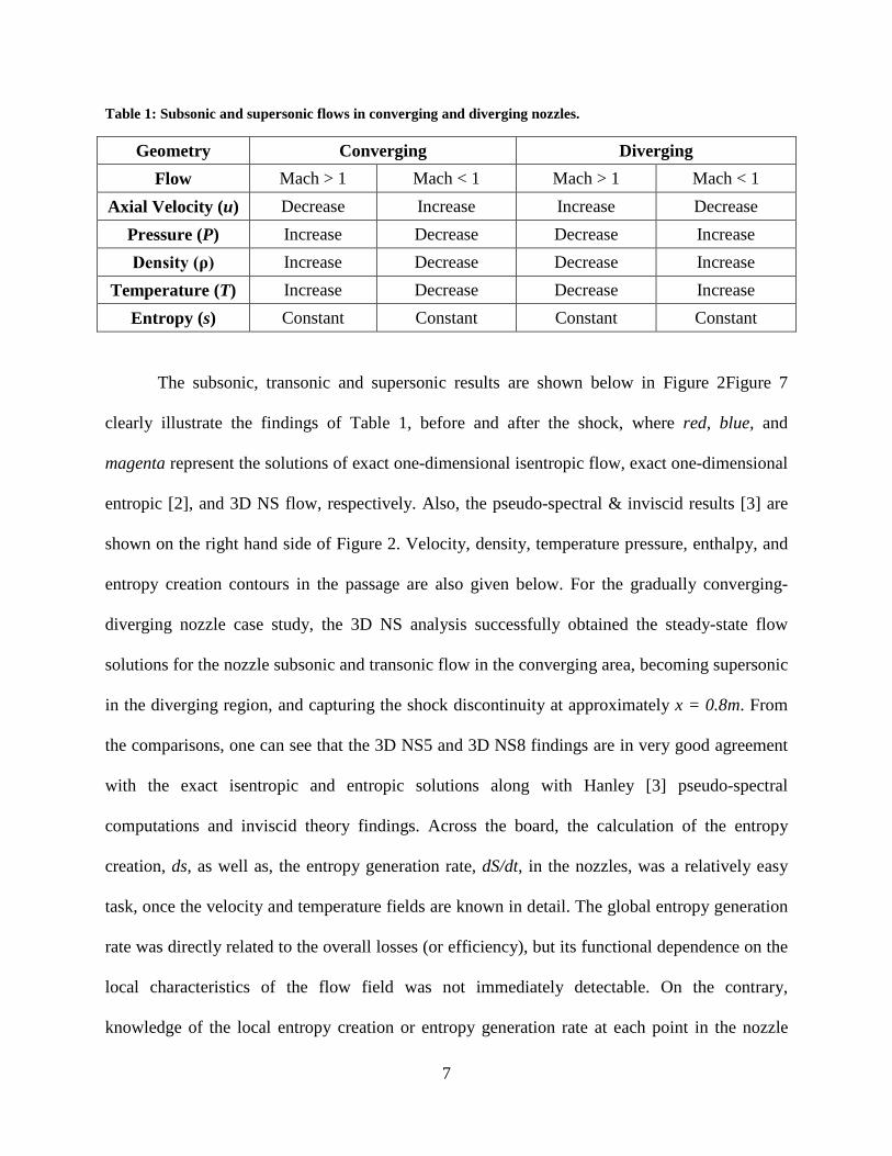
The subsonic, transonic and supersonic results are shown below in Figure 2Figure 7

clearly illustrate the findings of Table 1, before and after the shock, where red, blue, and

magenta represent the solutions of exact one-dimensional isentropic flow, exact one-dimensional

entropic [2], and 3D NS flow, respectively. Also, the pseudo-spectral & inviscid results [3] are

shown on the right hand side of Figure 2. Velocity, density, temperature pressure, enthalpy, and

entropy creation contours in the passage are also given below. For the gradually converging-

diverging nozzle case study, the 3D NS analysis successfully obtained the steady-state flow

solutions for the nozzle subsonic and transonic flow in the converging area, becoming supersonic

in the diverging region, and capturing the shock discontinuity at approximately x = 0.8m. From

the comparisons, one can see that the 3D NS5 and 3D NS8 findings are in very good agreement

with the exact isentropic and entropic solutions along with Hanley [3] pseudo-spectral

computations and inviscid theory findings. Across the board, the calculation of the entropy

creation, ds, as well as, the entropy generation rate, dS/dt, in the nozzles, was a relatively easy

task, once the velocity and temperature fields are known in detail. The global entropy generation

rate was directly related to the overall losses (or efficiency), but its functional dependence on the

local characteristics of the flow field was not immediately detectable. On the contrary,

knowledge of the local entropy creation or entropy generation rate at each point in the nozzle

8

provided immediate useful insight into the relative importance of the different sources of

irreversibility across the nozzle’s NS transport processes.

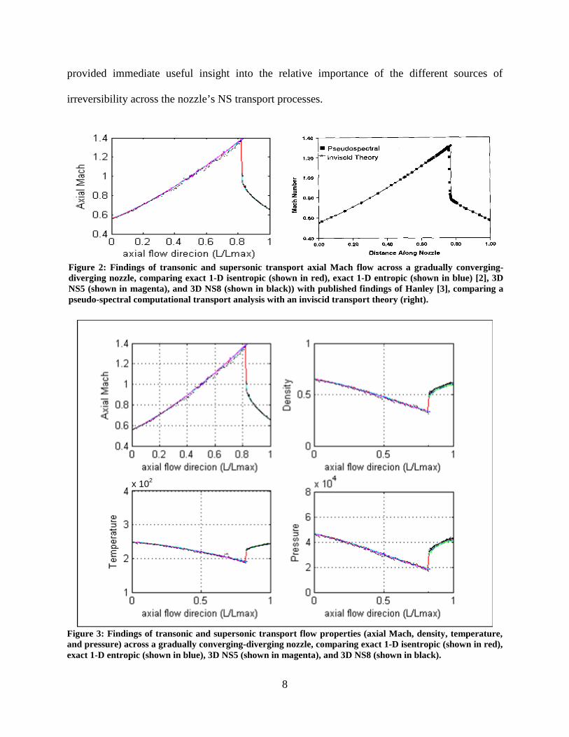
Figure 3: Findings of transonic and supersonic transport flow properties (axial Mach, density, temperature, and pressure) across a gradually converging-diverging nozzle, comparing exact 1-D isentropic (shown in red), exact 1-D entropic (shown in blue), 3D NS5 (shown in magenta), and 3D NS8 (shown in black).

x 102

Figure 2: Findings of transonic and supersonic transport axial Mach flow across a gradually converging-diverging nozzle, comparing exact 1-D isentropic (shown in red), exact 1-D entropic (shown in blue) [2], 3D NS5 (shown in magenta), and 3D NS8 (shown in black)) with published findings of Hanley [3], comparing a pseudo-spectral computational transport analysis with an inviscid transport theory (right).

9

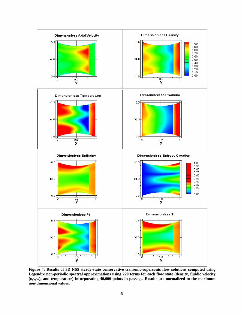
Figure 4: Results of 3D NS5 steady-state conservative transonic-supersonic flow solutions computed using Legendre non-periodic spectral approximations using 220 terms for each flow state (density, fluidic velocity (u,v,w), and temperature) incorporating 40,000 points in passage. Results are normalized to the maximum non-dimensional values.

10

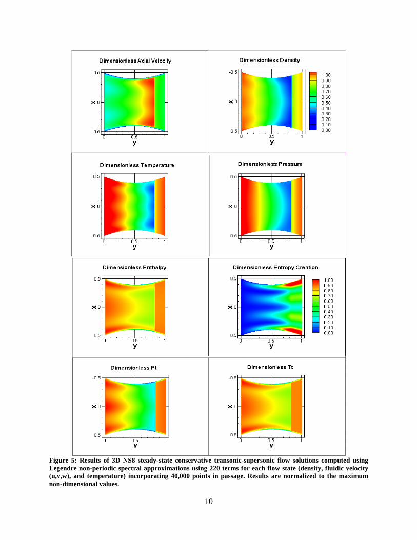
Figure 5: Results of 3D NS8 steady-state conservative transonic-supersonic flow solutions computed using Legendre non-periodic spectral approximations using 220 terms for each flow state (density, fluidic velocity (u,v,w), and temperature) incorporating 40,000 points in passage. Results are normalized to the maximum non-dimensional values.

11

Figure 6: Results of 3D NS5 steady-state conservative subsonic flow solutions computed using Legendre non-periodic spectral approximations using 286 terms for each flow state (density, fluidic velocity (u,v,w), and temperature) incorporating 64,000 points in passage. Results are normalized to the maximum non-dimensional values of ideal isentropic solution: Mach: 0.39; density: 0.65; temperature: 249; pressure: 4.7e+4; enthalpy (h): 2.5e+5; entropy creation (dS): 260.

12

Figure 7: Results of 3D NS8 steady-state conservative subsonic flow solutions computed using Legendre non-periodic spectral approximations using 286 terms for each flow state (density, fluidic velocity (u,v,w), and temperature) incorporating 64,000 points in passage. Results are normalized to the maximum non-dimensional values of ideal isentropic solution: Mach: 0.39; density: 0.65; temperature: 249; pressure: 4.7e+4; enthalpy (h): 2.5e+5; entropy creation (dS): 260.

13

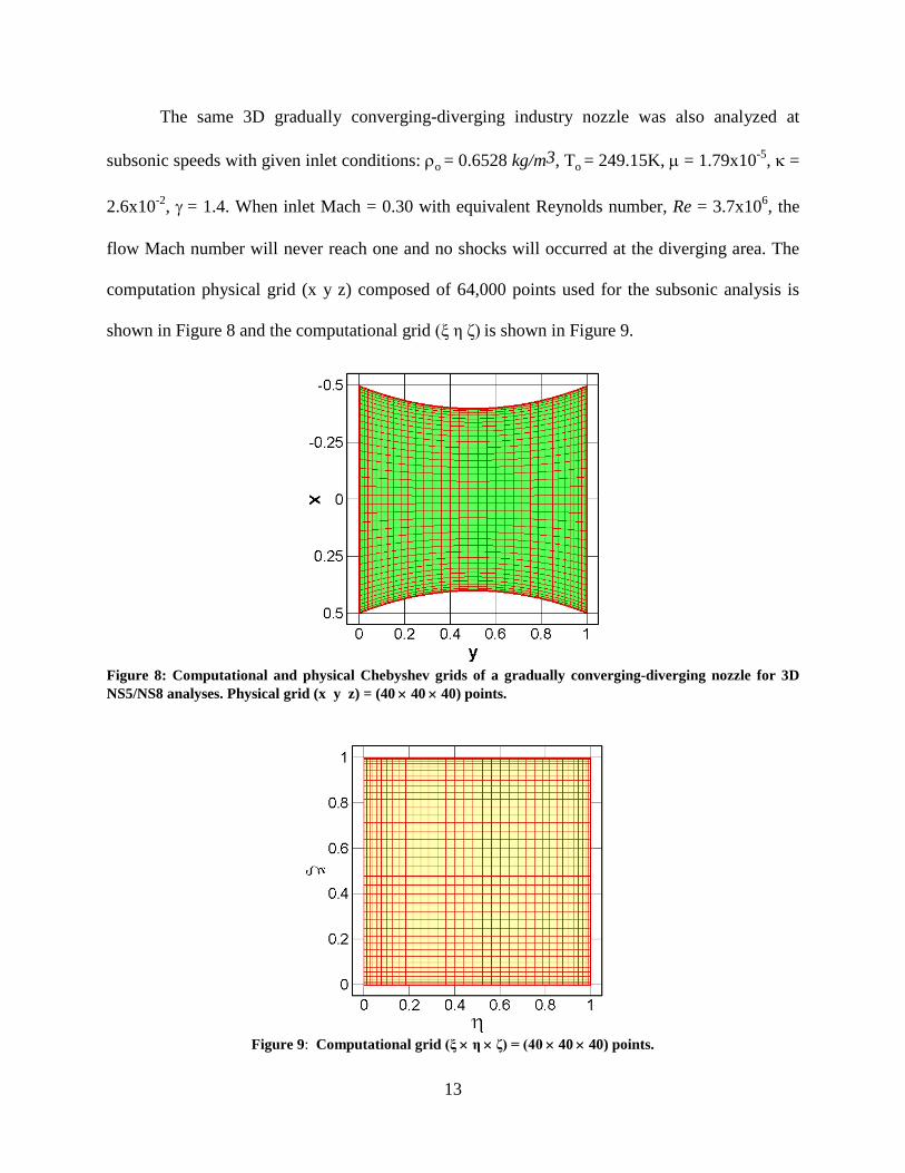
The same 3D gradually converging-diverging industry nozzle was also analyzed at

subsonic speeds with given inlet conditions: ρo = 0.6528 kg/m3, To = 249.15K, µ = 1.79x10-5, κ =

2.6x10-2, γ = 1.4. When inlet Mach = 0.30 with equivalent Reynolds number, Re = 3.7x106, the

flow Mach number will never reach one and no shocks will occurred at the diverging area. The

computation physical grid (x y z) composed of 64,000 points used for the subsonic analysis is

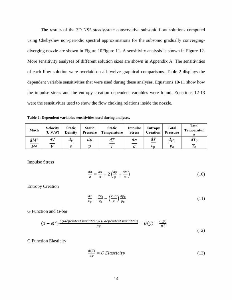
shown in Figure 8 and the computational grid (ξ η ζ) is shown in Figure 9.

Figure 8: Computational and physical Chebyshev grids of a gradually converging-diverging nozzle for 3D NS5/NS8 analyses. Physical grid (x y z) = (40 × 40 × 40) points.

Figure 9: Computational grid (ξ × η × ζ) = (40 × 40 × 40) points.

14

The results of the 3D NS5 steady-state conservative subsonic flow solutions computed

using Chebyshev non-periodic spectral approximations for the subsonic gradually converging-

diverging nozzle are shown in Figure 10Figure 11. A sensitivity analysis is shown in Figure 12.

More sensitivity analyses of different solution sizes are shown in Appendix A. The sensitivities

of each flow solution were overlaid on all twelve graphical comparisons. Table 2 displays the

dependent variable sensitivities that were used during these analyses. Equations 10-11 show how

the impulse stress and the entropy creation dependent variables were found. Equations 12-13

were the sensitivities used to show the flow choking relations inside the nozzle.

Table 2: Dependent variables sensitivities used during analyses.

Mach Velocity (U,V,W)

Static Density

Static Pressure

Static Temperature

Impulse Stress

Entropy Creation

Total Pressure

Total Temperatur

e 𝑑𝑀2

𝑀2 𝑑𝑉𝑉

𝑑𝜌𝜌

𝑑𝑝𝑝

𝑑𝑇𝑇

𝑑𝜎𝜎

𝑑�̅�𝑐𝑝

𝑑𝑝0𝑝0

𝑑𝑇0𝑇0

Impulse Stress

𝑑𝜎𝜎

= 𝑑κκ

+ 2 �𝑑𝑝𝑝

+ 𝑑𝑀𝑀� (10)

Entropy Creation

𝑑𝑠

𝐶𝑝= 𝑑𝑇0

𝑇0− �κ−1

𝜅� 𝑑𝑝0

𝑝0 (11)

G Function and G-bar

(1 −𝑀2) 𝑑(′𝑑𝑒𝑝𝑒𝑛𝑑𝑒𝑛𝑡 𝑣𝑎𝑟𝑖𝑎𝑏𝑙𝑒′ )/ (′ 𝑑𝑒𝑝𝑒𝑛𝑑𝑒𝑛𝑡 𝑣𝑎𝑟𝑖𝑎𝑏𝑙𝑒′)

𝑑𝑦= �̅�(𝑦) = 𝐺(𝑦)

𝑀2 (12)

G Function Elasticity

𝑑(�̅�)

𝑑𝑦= 𝐺 𝐸𝑙𝑎𝑠𝑡𝑖𝑐𝑖𝑡𝑦 (13)

15

Figure 10: Gradually Converging-Diverging subsonic flow nozzle Quasi 3D and 3D Steady-state solutions. (Red: Exact 1-D isentropic solutions; Orange: Exact 1-D entropic solutions; Blue: Quasi 3D NS3 solutions; Pink: Quasi 3D NS6 solutions; Green: 3D NS8 solutions). The Quasi 3D steady-state conservative subsonic flow solutions computed using Chebyshev 20th order non-periodic spectral approximations using 20 points in the passage with polynomials for each flow state (density, axial velocity (v), temperature, enthalpy, entropy, and heat transfer).

16

Figure 11: Results of 3D NS8 steady-state conservative subsonic flow solutions computed using Chebyshev non-periodic spectral approximations using 286 terms for each flow state (density, fluidic velocity (u,v,w), and temperature, enthalpy, entropy, and heat transfer) incorporating 64,000 points in passage. Results are normalized to the maximum non-dimensional values of ideal isentropic solution: Mach: 0.39; density: 0.65; temperature: 249; pressure: 4.7e+4; enthalpy (h): 2.5e+5; entropy creation (dS): 260.

17

Figure 12: Sensitivities of 3D NS5 steady-state conservative subsonic flow solutions using Chebyshev non-periodic spectral approximations using 286 terms for each flow state (density, fluidic velocity (u,v,w), and temperature) incorporating 64,000 points in passage. Results are normalized to the maximum non-dimensional values of the 3D NS5 solutions.

2.2 Venturi Tube

The second problem examined was venturi tube idealized as a 3D converging-diverging

nozzle, which introduces subsonic, transonic, and supersonic transport flow phenomena

including viscous boundary layer effects in a 3D unsteady NS analysis. Consider the 3D

converging-diverging industry nozzle shown in Figure 13 with given inlet conditions: To=2(103)

K, Po=10 atm. Mach number reaches unity at the throat area (y=0) with equivalent Reynolds

number Re = 3(107). A representative spectral idealization of the flow passage employed is

shown in Figure 14, which incorporates 40 sub-domains with a total 40(163) points used to

capture details of the unsteady, viscous transport flow processes.

18

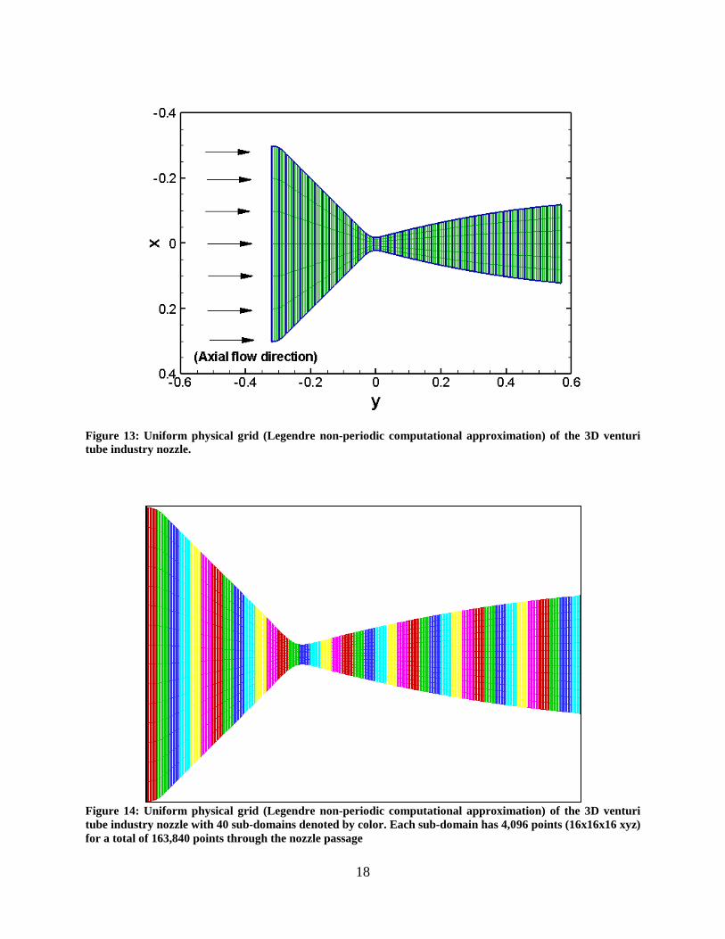
Figure 13: Uniform physical grid (Legendre non-periodic computational approximation) of the 3D venturi tube industry nozzle.

Figure 14: Uniform physical grid (Legendre non-periodic computational approximation) of the 3D venturi tube industry nozzle with 40 sub-domains denoted by color. Each sub-domain has 4,096 points (16x16x16 xyz) for a total of 163,840 points through the nozzle passage

19

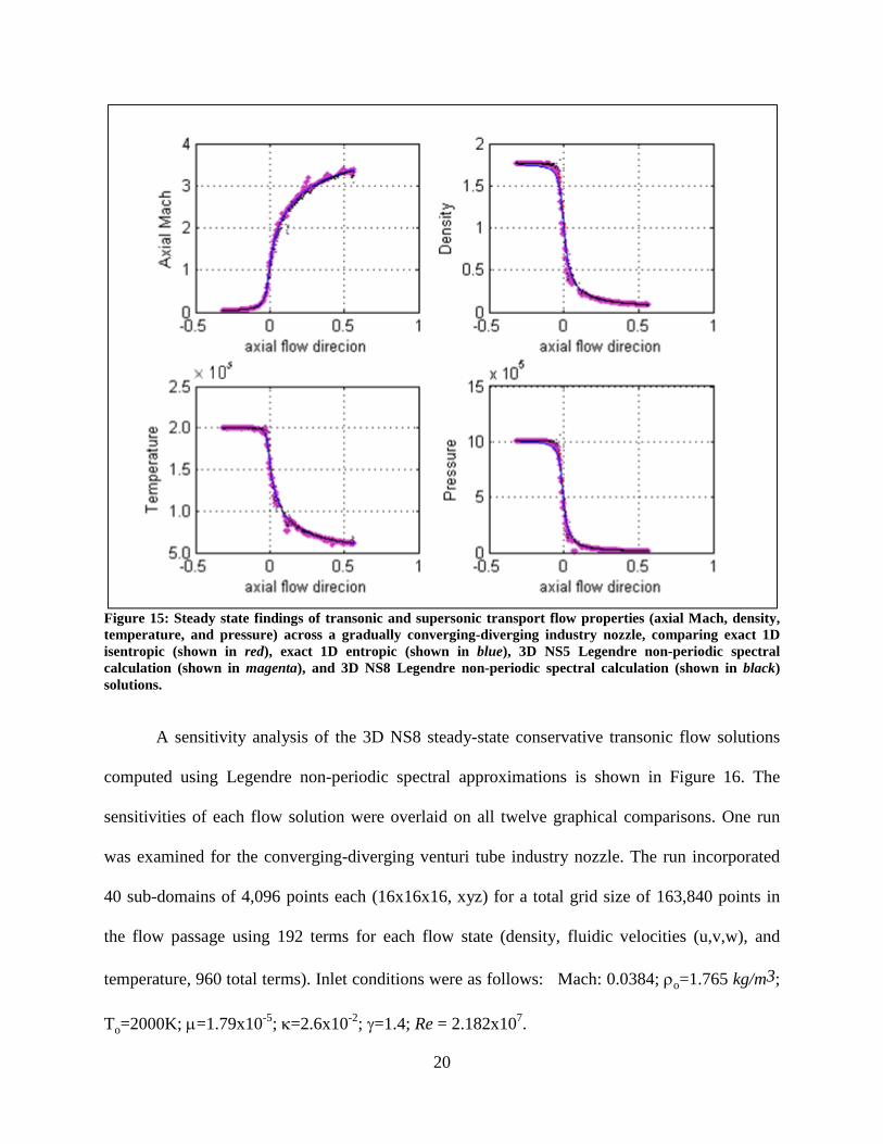
Steady state findings of transonic and supersonic transport flow solutions are shown in

Figure 15, where red, blue, and magenta colored data coinciding therein represent the solutions

of exact 1D isentropic, exact 1D entropic and unsteady 3D NS5 and 3D NS8 solutions,

respectively. The 3D NS solutions are transonic and supersonic flow of high Reynolds number

on the order of 107. The 3D NS solutions agree favorably with the exact isentropic and entropic

solutions. The results show the axial velocity in the nozzle accelerates past the Mach number of

unity at the throat area and gradually increases to supersonic Mach number well over 3 at the

outlet. Details of the 3D NS flow processes are summarized in the axial Mach, velocity, density,

temperature, and pressure contours through the nozzle passage shown in Appendix B. These

contours depict fundamentally not only how axial Mach velocity increases significantly and

consistently with density, temperature, and pressure drop across the nozzle passage, but also how

viscous boundary layer effects develop, and how convective heat transfer, that occurs between

the nozzle wall surface and the flowing fluid over it, advances particularly in the supersonic

diverging regions of the nozzle passage. The thermal effects of the nozzle surfaces on the

flowing fluid, like the viscous effects, are confined to a region near the surface that is thin

compared to the characteristic length of the nozzle surface, given the high Reynolds number on

the order of 107 treated in this industry nozzle case study. Generally speaking, the boundary layer

thickness relative to the characteristic length of the nozzle is at most proportional to the order of

(Re)-1/2 = (10)-7/2. In most of the components of such gas nozzle transport systems, analysts aim

to minimize viscous effects, working to achieve such high Reynolds numbers and thin boundary

layers, as predicted in Figure 16.

20

Figure 15: Steady state findings of transonic and supersonic transport flow properties (axial Mach, density, temperature, and pressure) across a gradually converging-diverging industry nozzle, comparing exact 1D isentropic (shown in red), exact 1D entropic (shown in blue), 3D NS5 Legendre non-periodic spectral calculation (shown in magenta), and 3D NS8 Legendre non-periodic spectral calculation (shown in black) solutions.

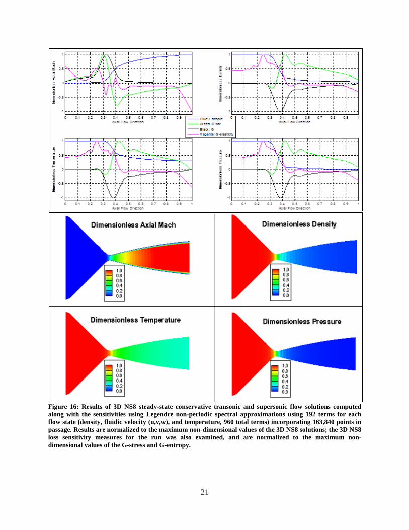
A sensitivity analysis of the 3D NS8 steady-state conservative transonic flow solutions

computed using Legendre non-periodic spectral approximations is shown in Figure 16. The

sensitivities of each flow solution were overlaid on all twelve graphical comparisons. One run

was examined for the converging-diverging venturi tube industry nozzle. The run incorporated

40 sub-domains of 4,096 points each (16x16x16, xyz) for a total grid size of 163,840 points in

the flow passage using 192 terms for each flow state (density, fluidic velocities (u,v,w), and

temperature, 960 total terms). Inlet conditions were as follows: Mach: 0.0384; ρo=1.765 kg/m3;

To=2000K; µ=1.79x10-5; κ=2.6x10-2; γ=1.4; Re = 2.182x107.

21

Figure 16: Results of 3D NS8 steady-state conservative transonic and supersonic flow solutions computed along with the sensitivities using Legendre non-periodic spectral approximations using 192 terms for each flow state (density, fluidic velocity (u,v,w), and temperature, 960 total terms) incorporating 163,840 points in passage. Results are normalized to the maximum non-dimensional values of the 3D NS8 solutions; the 3D NS8 loss sensitivity measures for the run was also examined, and are normalized to the maximum non-dimensional values of the G-stress and G-entropy.

22

2.3 Rectangular 90-Degree Bend Duct

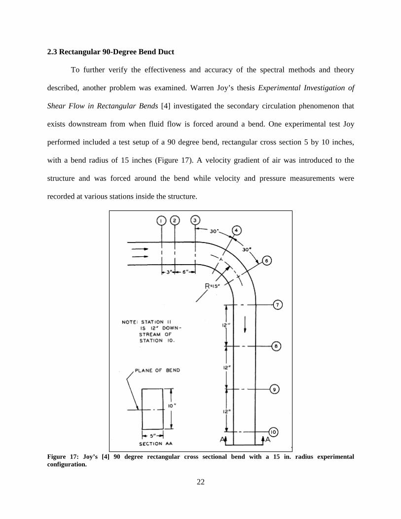
To further verify the effectiveness and accuracy of the spectral methods and theory

described, another problem was examined. Warren Joy’s thesis Experimental Investigation of

Shear Flow in Rectangular Bends [4] investigated the secondary circulation phenomenon that

exists downstream from when fluid flow is forced around a bend. One experimental test Joy

performed included a test setup of a 90 degree bend, rectangular cross section 5 by 10 inches,

with a bend radius of 15 inches (Figure 17). A velocity gradient of air was introduced to the

structure and was forced around the bend while velocity and pressure measurements were

recorded at various stations inside the structure.

Figure 17: Joy’s [4] 90 degree rectangular cross sectional bend with a 15 in. radius experimental configuration.

23

The stations indicted in the Figure 17 are where velocity measurements were taken to

analyze the flow going through the duct. Inlet flow conditions were 85 feet per second. The flow

started upstream far enough to have fully developed flow once the flow reached the start of the

bend (station 3). Joy’s experiment was designed to capture the evidence of secondary circulation

phenomena that occurs in rectangular cross sectional ducts downstream of bends. The results

obtained from Joy’s experiment can be seen in Figure 18.

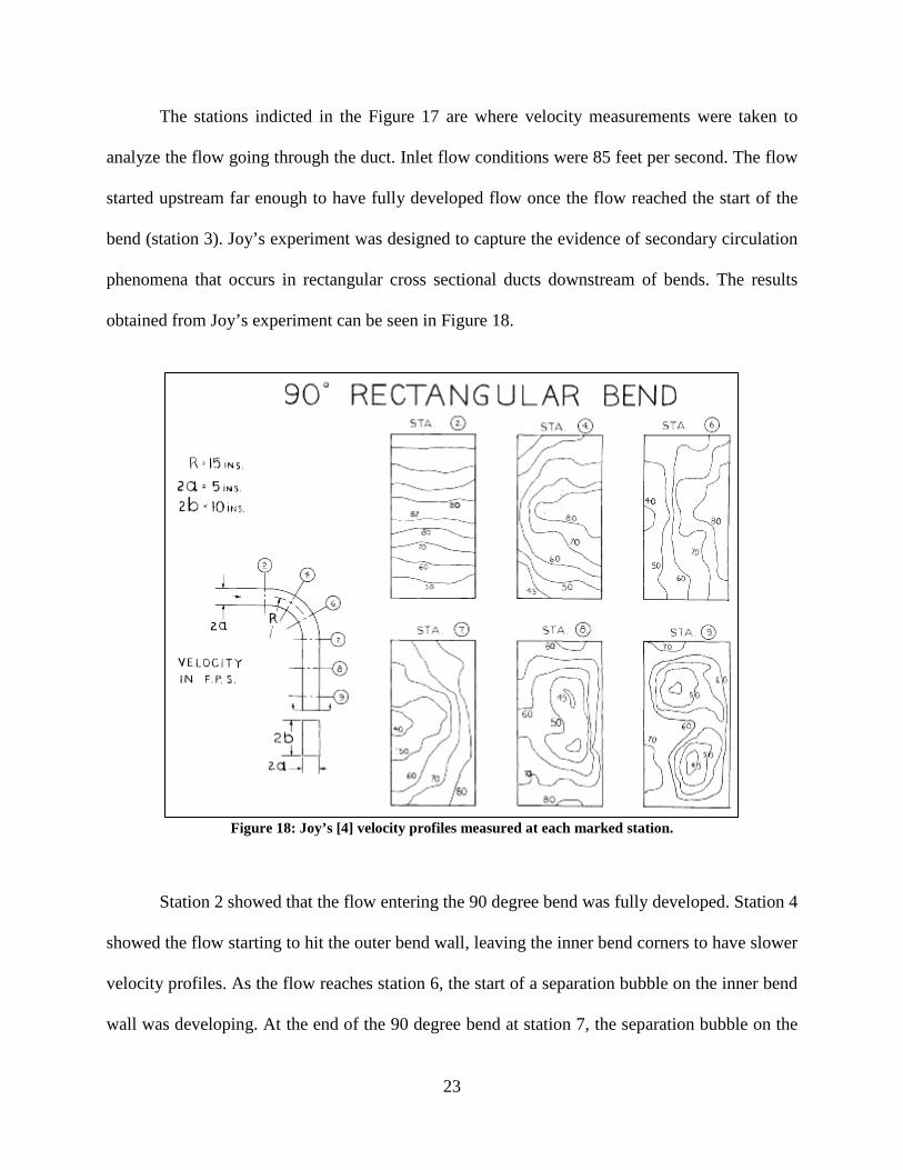
Figure 18: Joy’s [4] velocity profiles measured at each marked station.

Station 2 showed that the flow entering the 90 degree bend was fully developed. Station 4

showed the flow starting to hit the outer bend wall, leaving the inner bend corners to have slower

velocity profiles. As the flow reaches station 6, the start of a separation bubble on the inner bend

wall was developing. At the end of the 90 degree bend at station 7, the separation bubble on the

24

inner bend wall was more apparent and the faster velocity profile started to separate at the outer

bend wall. Station 8 showed the velocity profile starting to swirl displaying some evidence of

secondary circulation. The final station (station 9), 24 inches downstream from the end of the 90

degree bend, showed full evidence of secondary circulation which is displayed as two vortices in

the duct cross section.

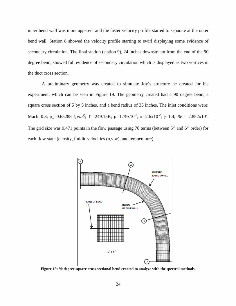
A preliminary geometry was created to simulate Joy’s structure he created for his

experiment, which can be seen in Figure 19. The geometry created had a 90 degree bend, a

square cross section of 5 by 5 inches, and a bend radius of 35 inches. The inlet conditions were:

Mach=0.3; ρo=0.65288 kg/m3; To=249.15K; µ=1.79x10-5; κ=2.6x10-2; γ=1.4; Re = 2.852x107.

The grid size was 9,471 points in the flow passage using 78 terms (between 5th and 6th order) for

each flow state (density, fluidic velocities (u,v,w), and temperature).

Figure 19: 90 degree square cross sectional bend created to analyze with the spectral methods.

25

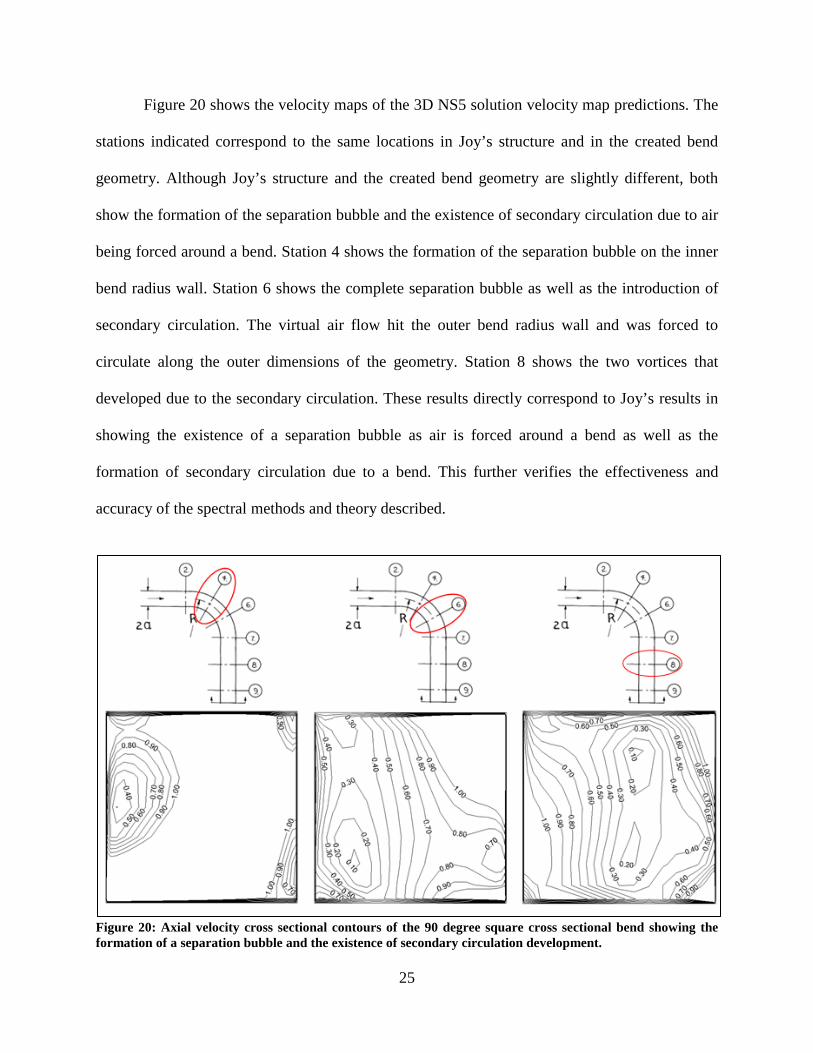
Figure 20 shows the velocity maps of the 3D NS5 solution velocity map predictions. The

stations indicated correspond to the same locations in Joy’s structure and in the created bend

geometry. Although Joy’s structure and the created bend geometry are slightly different, both

show the formation of the separation bubble and the existence of secondary circulation due to air

being forced around a bend. Station 4 shows the formation of the separation bubble on the inner

bend radius wall. Station 6 shows the complete separation bubble as well as the introduction of

secondary circulation. The virtual air flow hit the outer bend radius wall and was forced to

circulate along the outer dimensions of the geometry. Station 8 shows the two vortices that

developed due to the secondary circulation. These results directly correspond to Joy’s results in

showing the existence of a separation bubble as air is forced around a bend as well as the

formation of secondary circulation due to a bend. This further verifies the effectiveness and

accuracy of the spectral methods and theory described.

Figure 20: Axial velocity cross sectional contours of the 90 degree square cross sectional bend showing the formation of a separation bubble and the existence of secondary circulation development.

26

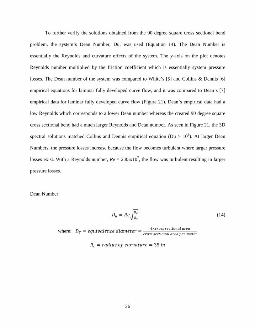
To further verify the solutions obtained from the 90 degree square cross sectional bend

problem, the system’s Dean Number, Du, was used (Equation 14). The Dean Number is

essentially the Reynolds and curvature effects of the system. The y-axis on the plot denotes

Reynolds number multiplied by the friction coefficient which is essentially system pressure

losses. The Dean number of the system was compared to White’s [5] and Collins & Dennis [6]

empirical equations for laminar fully developed curve flow, and it was compared to Dean’s [7]

empirical data for laminar fully developed curve flow (Figure 21). Dean’s empirical data had a

low Reynolds which corresponds to a lower Dean number whereas the created 90 degree square

cross sectional bend had a much larger Reynolds and Dean number. As seen in Figure 21, the 3D

spectral solutions matched Collins and Dennis empirical equation (Du > 103). At larger Dean

Numbers, the pressure losses increase because the flow becomes turbulent where larger pressure

losses exist. With a Reynolds number, Re = 2.85x107, the flow was turbulent resulting in larger

pressure losses.

Dean Number

𝐷𝑢 = 𝑅𝑒�𝐷𝐸𝑅𝑐

(14)

where: 𝐷𝐸 = 𝑒𝑞𝑢𝑖𝑣𝑎𝑙𝑒𝑛𝑐𝑒 𝑑𝑖𝑎𝑚𝑒𝑡𝑒𝑟 = 4×𝑐𝑟𝑜𝑠𝑠 𝑠𝑒𝑐𝑡𝑖𝑜𝑛𝑎𝑙 𝑎𝑟𝑒𝑎𝑐𝑟𝑜𝑠𝑠 𝑠𝑒𝑐𝑡𝑖𝑜𝑛𝑎𝑙 𝑎𝑟𝑒𝑎 𝑝𝑒𝑟𝑖𝑚𝑒𝑡𝑒𝑟

𝑅𝑐 = 𝑟𝑎𝑑𝑖𝑢𝑠 𝑜𝑓 𝑐𝑢𝑟𝑣𝑎𝑡𝑢𝑟𝑒 = 35 𝑖𝑛

27

Figure 21: Comparison of pressure loss versus Reynolds curvature effect of experimental results of White’s [5], Collins and Dennis [6], and Dean’s [7] empirical equations for laminar fully developed curved flow.

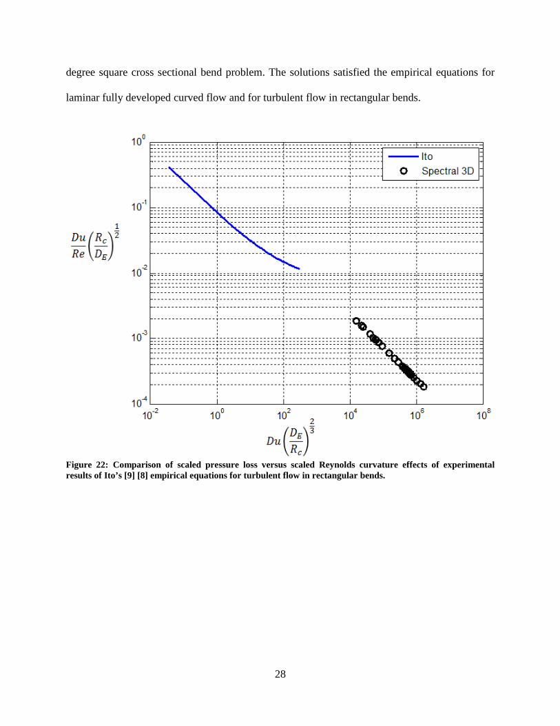
Furthermore, the 3D spectral solutions for the 90 degree square cross sectional bend

problem was matched against Ito’s [8] [9] empirical equation for turbulent flow in rectangular

bends (Figure 22). The plot is a comparison of the scaled pressure loss versus the scaled

Reynolds curvature effects. As seen from the plot, 3D spectral solutions for the bend problem

examined, showed the same form as Ito’s equation as if it were an extension to the equation

(higher scaled Reynolds curvature effects). The bend problem examined had turbulent flow

present due to the large inlet velocity introduced into the bend. The relationships highlighted in

Figure 21Figure 22 shows that the 3D spectral solutions obtained are correct solutions for the 90

28

degree square cross sectional bend problem. The solutions satisfied the empirical equations for

laminar fully developed curved flow and for turbulent flow in rectangular bends.

Figure 22: Comparison of scaled pressure loss versus scaled Reynolds curvature effects of experimental results of Ito’s [9] [8] empirical equations for turbulent flow in rectangular bends.

29

Chapter 3: Conclusion and Future Work After taking a step back and analyzing the three problems mentioned in this thesis, the

converging-diverging nozzle, the venturi tube industry nozzle, and the rectangular 90-degree

bend duct, the ROM analysis developed has been verified to be working effectively and

accurately in obtaining close-form solutions to steady advection-diffusion, unsteady convection-

diffusion, and unsteady compressible viscous flow problems. The three problems were chosen

specifically to analyze different geometry affects that when combined are similar to

turbomachinery problems. One flow domain between a set of rotor blades is very similar to a

converging-diverging nozzle problem along with a bend problem. The developed ROM analysis

obtained correct solutions for these problems; therefore it can be used for turbomachinery

applications.

Future work would entail analyzing NASA test rotor 67 along with other NASA test

rotors, standard configuration rotors, and other multistage rotor/stator turbomachines that have

experimental test data available to the science community. If the ROM analysis proves to be

effective and efficient in obtaining accurate results to turbomachinery problems, it can become a

powerful tool that can help the aerospace industry in analyzing jet engines. Loss mechanisms

will be predicted inside a jet engine before the engine is even made, which will help engineers

and scientists develop better and more advanced jet engines.

Spectral technologies are not a new analysis that is going to replace conventional CFD

methodologies, but another analysis that will complement conventional CFD methodologies in

analyzing turbomachinery. More research needs to be performed on spectral technologies to

catch up with conventional CFD methodologies to prove to be useful along with conventional

30

CFD methodologies. The future of CFD may involve some type of combination of spectral

technologies with conventional CFD methodologies. Only time will tell.

31

References

[1] R. V. Chima, "Viscous Three-dimensional Calculationss of Transonic Fan Performance," in CFD Techniques for Propulsion Applications, AGARD Conference Proceedings No. CP-510, Neuilly-Sur-Seine, France, 1992.

[2] J. E. A. John, Gas Dynamics, 2nd ed. Prentice Hall, Englewood Cliffs, NJ, 1984.

[3] P. Hanley, "A Strategy for the Efficient Simulation of Viscous Compressible Flows using a Multi-domain Pseudospectral Method," Journal of Computational Physics, vol. 108, pp. 153-158, September 1993.

[4] W. Joy, Experimental Investigation of Shear FLow in Rectangular Bends, MIT Master's Thesis, 1950.

[5] C. M. White, "Streamline Flow Through Curved Pipes," Proc. Royal Society A, 123, pp. 645-663, 1929.

[6] W. N. Collins, "The Steady Motion of a Viscous Fluid in a Curved Tube," Quart J. Mech. Appl. Math, vol. 28, no. 2, pp. 133-156, 1975.

[7] W. R. Dean, "Note on the Motion of Fluids in a Curved Pipe," Phil. Mag. Ser. 7, vol. 4, no. 20, pp. 208-223, 1927.

[8] H. Ito, "Theory on Laminar Flows through Curved Pipes, Elliptic and Rectangular Cross Sections," High Speed Mech. Tohoku University, Japan 1, pp. 1-16, 1951.

[9] H. Ito, "Friction Factor for Turbulent Flows in Curved Pipes," Trans. ASME, Ser. D, 81, pp. 123-134, 1959.

32

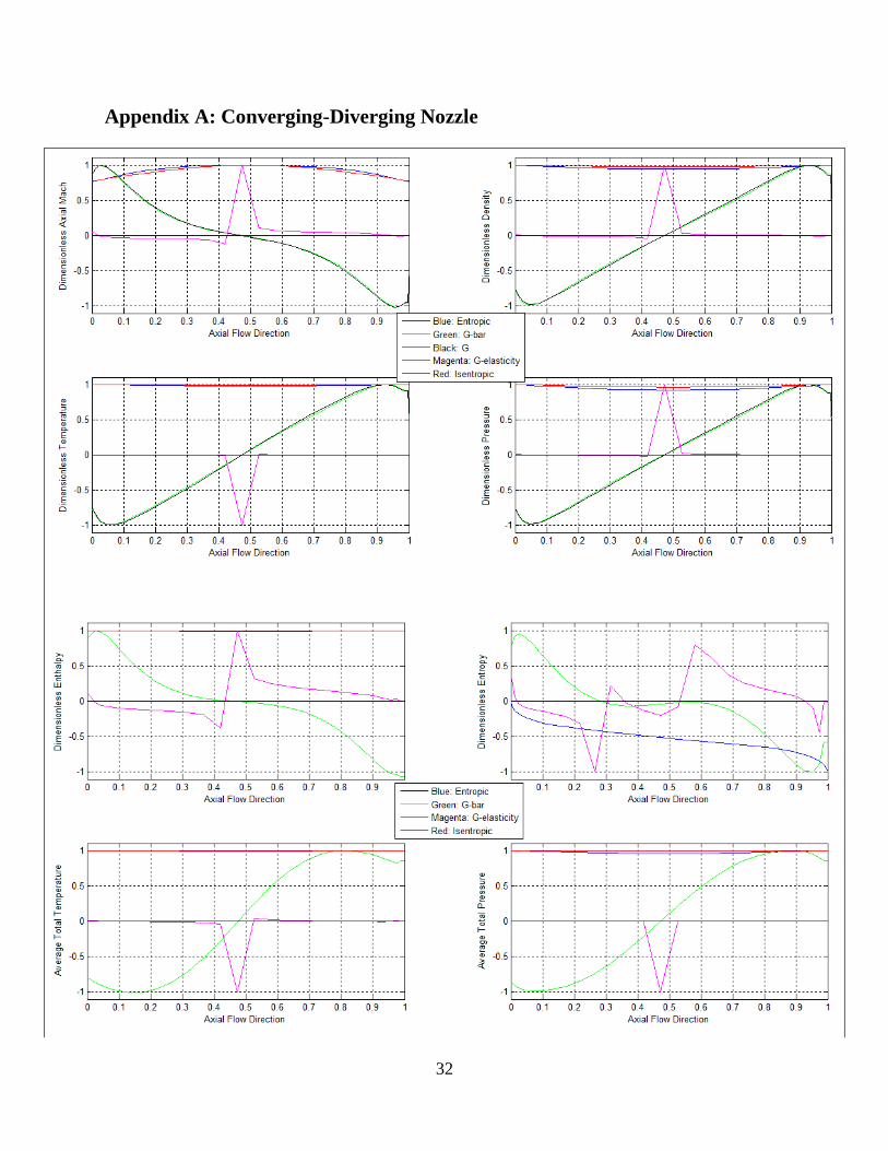
Appendix A: Converging-Diverging Nozzle

33

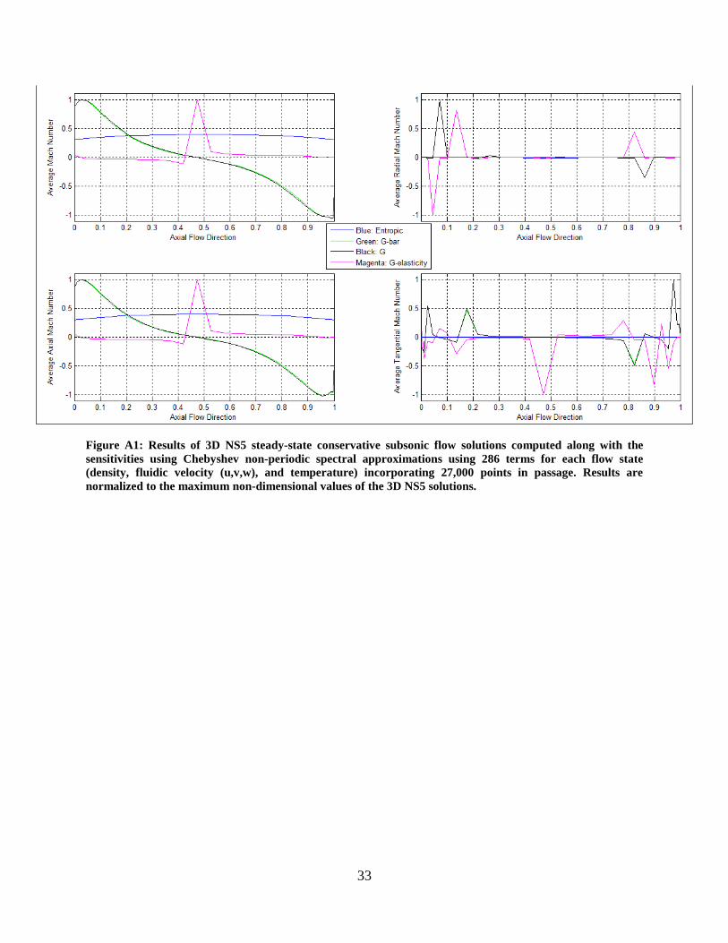
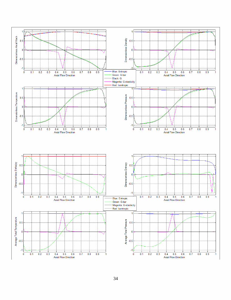
Figure A1: Results of 3D NS5 steady-state conservative subsonic flow solutions computed along with the sensitivities using Chebyshev non-periodic spectral approximations using 286 terms for each flow state (density, fluidic velocity (u,v,w), and temperature) incorporating 27,000 points in passage. Results are normalized to the maximum non-dimensional values of the 3D NS5 solutions.

34

35

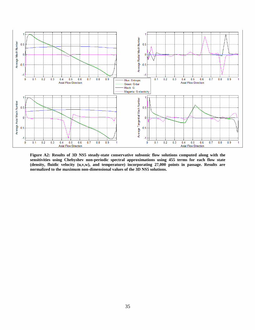
Figure A2: Results of 3D NS5 steady-state conservative subsonic flow solutions computed along with the sensitivities using Chebyshev non-periodic spectral approximations using 455 terms for each flow state (density, fluidic velocity (u,v,w), and temperature) incorporating 27,000 points in passage. Results are normalized to the maximum non-dimensional values of the 3D NS5 solutions.

36

37

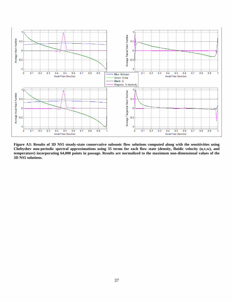
Figure A3: Results of 3D NS5 steady-state conservative subsonic flow solutions computed along with the sensitivities using Chebyshev non-periodic spectral approximations using 35 terms for each flow state (density, fluidic velocity (u,v,w), and temperature) incorporating 64,000 points in passage. Results are normalized to the maximum non-dimensional values of the 3D NS5 solutions.

38

39

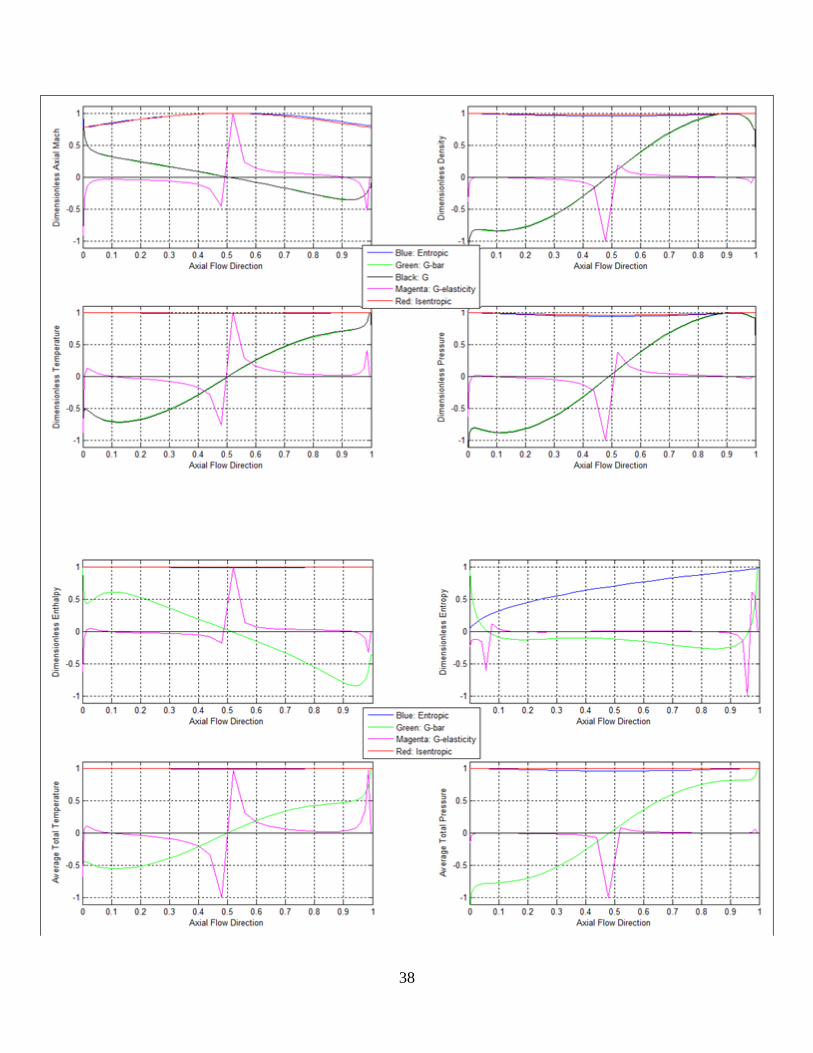
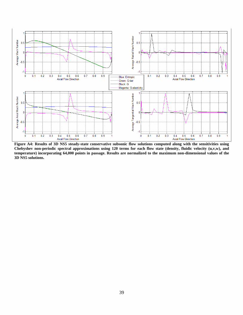
Figure A4: Results of 3D NS5 steady-state conservative subsonic flow solutions computed along with the sensitivities using Chebyshev non-periodic spectral approximations using 120 terms for each flow state (density, fluidic velocity (u,v,w), and temperature) incorporating 64,000 points in passage. Results are normalized to the maximum non-dimensional values of the 3D NS5 solutions.

40

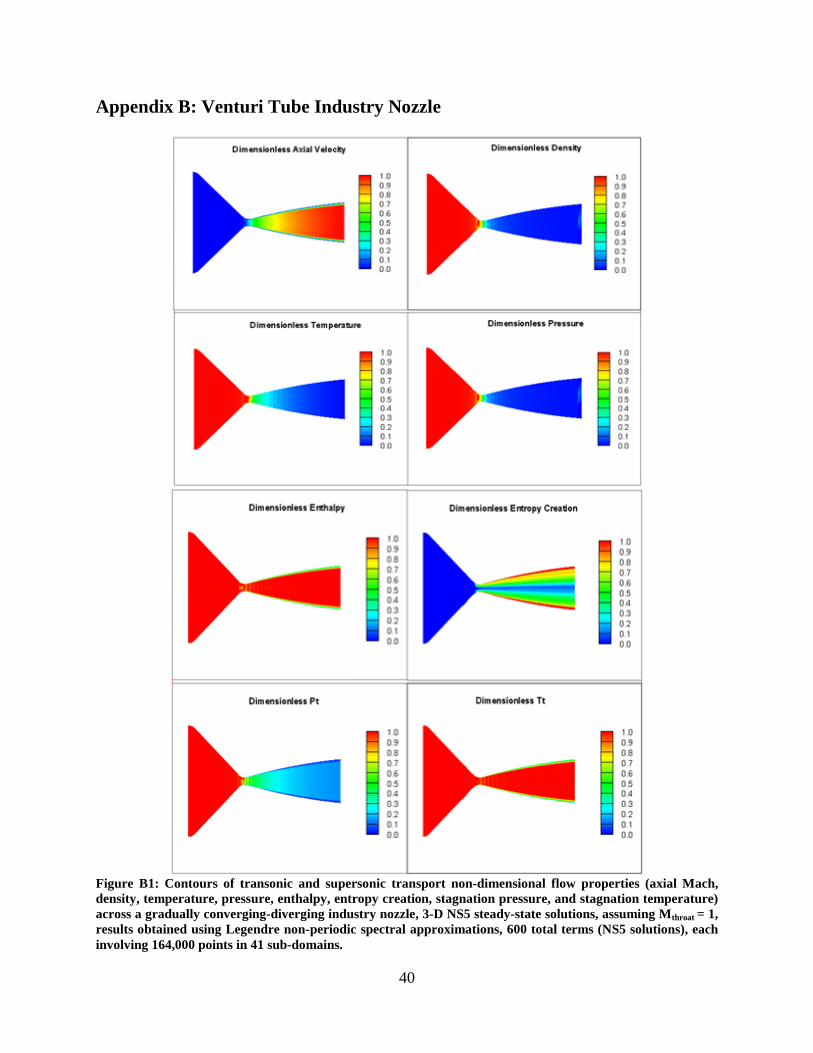
Appendix B: Venturi Tube Industry Nozzle

Figure B1: Contours of transonic and supersonic transport non-dimensional flow properties (axial Mach, density, temperature, pressure, enthalpy, entropy creation, stagnation pressure, and stagnation temperature) across a gradually converging-diverging industry nozzle, 3-D NS5 steady-state solutions, assuming Mthroat = 1, results obtained using Legendre non-periodic spectral approximations, 600 total terms (NS5 solutions), each involving 164,000 points in 41 sub-domains.

41

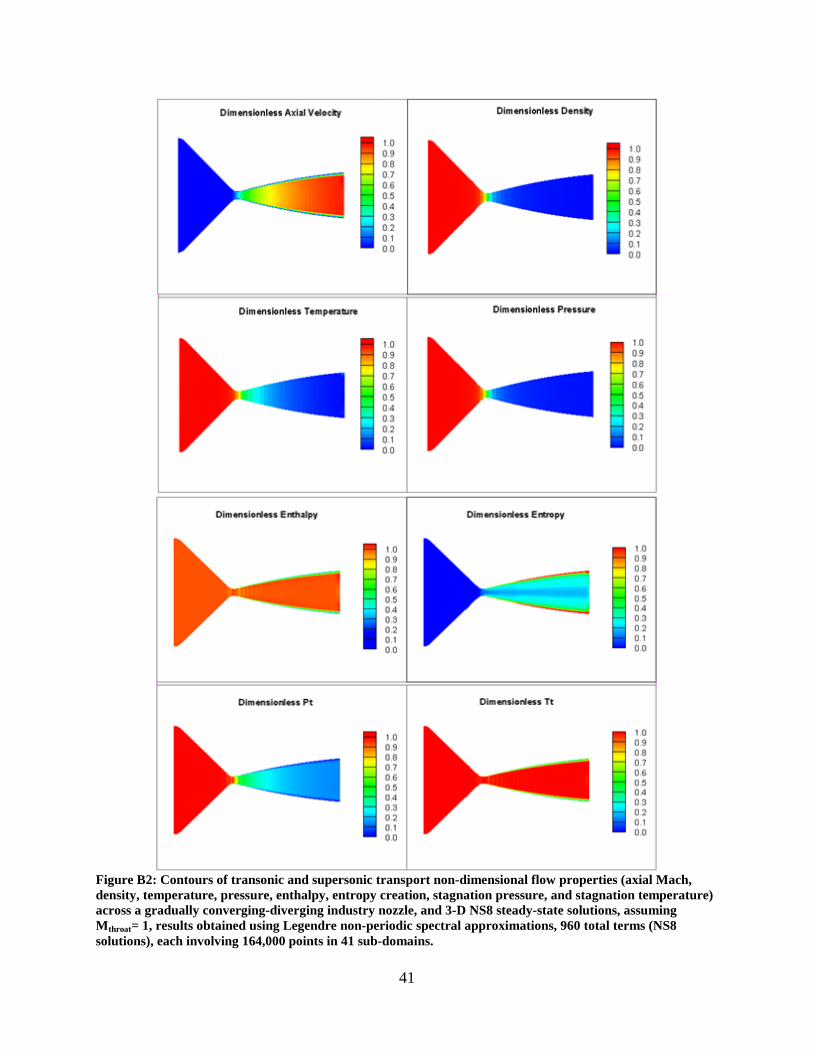
Figure B2: Contours of transonic and supersonic transport non-dimensional flow properties (axial Mach, density, temperature, pressure, enthalpy, entropy creation, stagnation pressure, and stagnation temperature) across a gradually converging-diverging industry nozzle, and 3-D NS8 steady-state solutions, assuming Mthroat= 1, results obtained using Legendre non-periodic spectral approximations, 960 total terms (NS8 solutions), each involving 164,000 points in 41 sub-domains.