The Value of Quality Improvements

Djoko Setijono1 and Jens J. Dahlgaard2

1Department of Forest & Wood Technology, School of Technology & Design

Växjö University, Sweden 2Division of Quality Technology and Management, Department of Management

and Engineering, Linköping University, Sweden

djoko.setijono@vxu.se jens.jorn.dahlgaard@liu.se

Abstract Purpose - To present a proactive quality costs measurement methodology, which describes the value of quality improvements and the implication of this value on customers' perception regarding the value of the product. Design/methodology/approach - By describing the perceived customer value in a dynamic term, it becomes possible to derive an analytical model that recognizes the implication of a company's efforts to improve design quality and conformance quality on product value as perceived by the customers. Quality costs as a performance indicator of improved design quality and conformance quality (as the results of prevention and appraisal activities) can be expressed in terms of value (i.e. a trade-off between benefits and sacrifices), where the benefits of the improvement include higher product quality and reduction of failure costs. The sacrifices include the costs to perform improvement activities (i.e. prevention and appraisal costs). Expressing quality costs in this way thus establishes a link between producer's efforts to improve quality and the way customers perceive the value of the product. The developed methodology of proactive quality cost measurement has been applied for collecting, measuring, and reporting quality costs in a Swedish wood-flooring manufacturing company. Findings - Transforming quality cost measurements into value provides a better explanation regarding the effect of prevention and appraisal activities on the quality improvement indicators. Thus, the value of quality improvements is a measure of return on quality improvements (ROQI), which indicates whether the quality improvement efforts gave higher, fair, or lower return. Originality/value - This paper develops and discusses a model of customer value by accommodating its relative-nature, and presents a proactive way of measuring quality costs (i.e. value-oriented and customer-oriented). Keywords Proactive quality cost, value, return on quality improvements. Paper type Research paper. Introduction Quality cost is a well-known concept in the area of quality management and gains much attention from the academic society as well as companies, consultants, etc. However, most of the authors discuss the subject of defining and categorizing quality cost but skip over the subject of gathering/measuring (Williams et al, 1999; Mandal and Shah, 2002). In practice, few companies have established systems for collecting the required cost elements, which probably is caused by a lack of systematic methodologies for collection, measurement, and reporting (Shah and Fitzroy, 1998).

1

The existing concept of quality costs itself has been criticized as: 1) it is reactive

rather than proactive, i.e. deals with the consequences of failures and losses, 2) it is based on producer's way of defining quality and it does not adequately take customers' perspectives into account (Moen, 1998). Gryna (1977; in Juran, 1998) tried to solve problem (2) through the development of a user's quality cost definition, but was criticised that it was still reactively defined.

Roden and Dale (2000) state that the value of conducting a quality cost analysis

is through highlighting non-value adding activities or waste and pinpointing potential improvements. According to Dahlgaard et al (1992), quality costs are an indicator (or a measure) of the effectiveness of a quality management system, and the identification of potential failures lead to the identification of improvement opportunities. Conti (1993) states that using only quality costs for improvement is inadequate; it is necessary to broaden the narrow perspective of quality costs into a customer value analysis to capture a broader impact of quality and adopt a continuous improvement approach to "sense" the improvement opportunities.

We may capture the messages above that: 1) there is a need for a systematic

quality cost collection, measurement, and reporting system, as well as 2) there is a need to develop quality cost measurements in a proactive way, i.e. to consider the customer's perspective, which often either may be difficult to measure or is unknown. Hence, the purpose of this paper is to suggest a proactive quality cost measurement methodology as a mechanism to indicate if quality improvements are valuable in the sense that the producer's efforts (activities) to improve quality will likely affect customers' perceptions about the value of the product. Thus, it encourages awareness that producers have active roles (e.g. capturing, interpreting, and improving) in customer value creation.

After a literature review, the authors present a model of dynamic customer value

and the producer's way of viewing and influencing customer value, followed by the description of a methodology for systematically collecting, measuring, and reporting quality costs. Next, the paper presents a case study in a Swedish wood-flooring manufacturer, where quality costs were identified and measured using the new methodology, and the applicability of proactive quality cost measurements. After discussion of the results and the findings, the authors finalise with conclusions. Literature review on quality cost Definitions of quality cost Juran (1951; in Dahlgaard, 1998) first defined quality cost as the cost, which would disappear if no defects were produced. This definition was redefined, by Juran after 38 years, as the cost of poor quality is the sum of all cost that would disappear if there were no quality problems. According to Besterfield (1994; in Chiadamrong, 2003), quality costs are those costs associated with the non-achievement of product or service quality as defined by the requirements established by the company and its contract with customers and society. All these definitions view quality cost as the consequence of failures or problems.

A “wider” interpretation of quality cost can be found in the definition that quality

cost is the cost in ensuring and assuring quality as well as loss incurred when quality

2

is not achieved - BS 6143 part 2 (see e.g. Dale and Plunkett, 1999) or the expenditure incurred in defect prevention and appraisal activities plus the losses due to internal and external failure - BS 4778 part 2 (see e.g. Dale and Plunkett, 1999).

Campanella (1990; in Dahlgaard et al, 1998) presented another version of quality

cost as the sum of prevention, appraisal, and failure costs that represents the difference between the actual cost of a product or service, and what the reduced cost would be if there was no possibility of substandard service, failure of product, or defects in their manufacture.

The definition of quality cost in Kolarik (1995) is probably the most appropriate

to “integrate” the different definitions above. Kolarik defines quality cost as any cost that result from the fact that systems (including people), processes, products, and services are imperfect. Models and definitions of quality cost elements According to Feigenbaum (1956, 1991), quality costs include two principal areas, i.e. the cost of control and the costs of failure of control. The costs of control are measured in two segments: prevention costs and appraisal costs, and the costs of failure of control consist of internal failure costs and external failure costs.

Prevention cost is the cost or investment of any action taken to investigate,

prevent, or reduce the risk of non-conformity (BS 6143 part 2, in Dale and Plunkett, 1999) or errors from occurring in all functions within the company (Omachonu et al, 1994). Prevention cost reflects the upfront investment of time and effort to prevent a problem from occurring (Millar, 1999); it seeks to eliminate the opportunity for quality defects (Angell and Chandra, 2001).

Appraisal cost is the cost of evaluating the achievement of quality requirements

including e.g. cost of verification and control performed at any stage of the quality loop (BS 6143: part 2) whenever there exists a chance for poor quality (Angell and Chandra, 2001) incurred before shipment of the product (Omachonu, 2004).

Internal failure cost is the cost arising within an organization due to non-

conformities at any stage of the quality loop such as costs of scrap, rework, retest, re-inspection, and redesign (BS 6143: part 2, in Dale and Plunkett, 1999; Morse, 1993; in Angell and Chandra, 2001). It is the result of quality failures or defective goods found within the company before shipment to customers (Millar, 1999; Angell and Chandra, 2001; Omachonu, 2004).

External failure cost is the cost arising after delivery to customers/users due to

non-conformities or defects which may include the cost of claims against warranty, replacement and consequential losses and evaluation of penalties required (BS 6143: part 2, in Dale and Plunkett, 1999). It is the cost resulting from products not conforming to customer requirements (Millar, 1999) or cost associated with defects that are found after the products are shipped to the customers (Angell and Chandra, 2001; Omachonu, 2004).

Several authors have proposed models of quality cost, e.g. Dahlgaard et al (1992)

and Dahlgaard et al (1998) suggest that quality cost can be classified in two

3

dimensions, with internal and external quality costs on the one dimension and visible and invisible quality costs on the other dimension; Sandoval-Chavez and Beruvides (1998) add opportunity cost into the PAF (Prevention-Appraisal-Failures) model; Chiadamrong et al (2003) propose that total quality cost is the sum of production-invisible quality costs, visible quality costs, and opportunity cost. Other models such as time-based cost element method and semi-structured identification and measurement methods, i.e. department based quality cost analysis method, team-based quality cost analysis, and a process cost model have been described in Dale and Plunkett (1999).

Carr and Ponomeon (1994; in Omachonu et al, 2004) suggest that internal failure

is the most expensive and prevention is the least expensive quality cost component. Omachonu et al (2004) suggest that prevention activities have a direct and positive influence on the profit margin and the company should not exclusively invest in appraisal because it may lead to unacceptable costs and may affect the company's reputation. The failure costs are usually much higher than prevention and appraisal costs, and failure costs have a negative correlation with the level of quality.

Tsai (1998) "initiates" the effort of identifying the link between quality cost and

value by classifying the quality cost elements into "value-added" and "non value-added" based on Activity Based Costing (ABC). Although the model indicates value added (-ness), there is no reference to customer value neither the effect of those value-added (-ness) on customer value. He also highlights that the PAF and the ABC models are related, where prevention and appraisal costs are value-added quality costs and failure costs are non-value added quality costs. The use of quality cost Quality cost can be used to capture top management’s attention for quality programs (Angell and Chandra, 2001) to indicate the quality level (Chen and Weng, 2002) and the symptom of problems (Millar, 1999). It is an important aspect of the development of a quality system (Dahlgaard et al, 1992) and a foundation for building a quality culture and implementing TQM as well as sophisticating the quality culture and management in term of practices (Prickett and Rapley, 2001; Mandal and Shah, 2002). The use of quality cost usually leads to the identification, selection, priority, measurement, evaluation, and monitoring of quality improvements (Keogh et al, 1998; Dale and Plunkett, 1999; Williams et al, 1999; Angell and Chandra, 2001), which is found to be very beneficial for continual improvement at the beginning of a quality journey (Tatikonda and Tatikonda, 1996; in Angell and Chandra, 2001).

According to Dale and Plunkett (1999), quality cost is a business parameter and a

performance measure that can be used as a means for planning and controlling future quality costs (see also the "quality cost thermometer", implemented in Milliken Denmark A/S (in Dahlgaard et al, 1998)). Omachonu et al (2004) state that a quality cost system can be established in an attempt to increase the value of the product and process output, and enhance customer satisfaction.

Juran (1951) states that the purpose of quality management is to satisfy customer

requirements through quality of design and quality of production (conformance to specifications), or similar to Ishikawa's forward-looking and backward-looking quality (see Kondo, 1993). The existing concept of quality costs is very much

4

influenced by conformance quality or backward-looking (must-be) quality but is less influenced by design quality or forward-looking (attractive) quality. Hence, quality costs depend on how the quality is defined and who (producer or customer) defines it. Therefore, quality cost normally presents a measure seen from the producer's perspective but seldom from the customer's perspective.

In order to capture the "true essence" of quality, it is suggested that quality costs

should be put in another context and measured in a new way, i.e. in terms of value. By doing so, the measurements can be used to model the contribution of improvements on the change in customer value. Customer value and its dynamic model Customer value Customer value is a trade-off (in terms of a difference or a ratio) between benefits and sacrifices (Dumond, 2000; Khalifa, 2004). The customers may be willing to sacrifice a certain amount of time, effort, money, and risk in exchange of expected benefits such as utility value and/or psychic value (Khalifa, 2004). When the benefits are expected to be higher than the sacrifices, then the customers may decide to purchase the product.

According to Bounds et al (1994), customer value is both idiosyncratic

(personally determined) and relative (changing over time). Most of the models that explain the concept and definition of customer value emphasize the idiosyncratic nature of customer value but there is not much emphasis on the relative nature because accommodating the relative nature of customer value into a model is not a simple task. The idiosyncratic and relative natures make customer value subjective, ambiguous, and difficult to define (Khalifa, 2004).

A dynamic model of customer value In this paper, a model to accommodate the relative nature of customer value is proposed, with the assumptions that: 1) the model is to be used to describe the effect of continuous improvements on customer value, and 2) the main focus is on customer value in the acquisition context, or as Gale (1994) refers as perceived customer value, which is defined as a ratio between market perceived quality (MPQ) and market perceived price (MPP).

The dynamic model of perceived customer value (PCV) can be expressed as:

PCVii RPCVPCV *1 =+ (1) Where: PCVi : Perceived customer value at time i

RPCV : The relative change in PCV from time i to (i+1), stated as i

i

PCVPCV 1+

Customer value is indeed changing over time, and people's perceptions about the value of a product can only be measured at a certain point in time. Since customer value is also idiosyncratic in its nature, the customer is the only entity that knows exactly the way he/she perceives the value of a product. Other entities, such as the producer, can only estimate (approximate) customers' minds (perceptions) regarding

5

the value of a product. However, producer's activities have significant effects on customers' perceptions regarding the value of the product. In the following sections, the producer's way of viewing and influencing customer value will be discussed and defined.

Producer's view (interpretation) of customer perceived value The producer may face another difficulty on the attempt to predict the PCV because the PCV is an abstract (intangible) matter and may be difficult to understand. According to Conti (2005), an economic relation (i.e. the relation between seller and purchaser in the purchasing-context) always implies the relation between the purchaser and the "object" of transaction (product) in order to appreciate the object's value [in a monetary term].

The interpretation would then be that the seller (whom might be the producer as well) recognizes the amount of money paid by the purchaser as an indicator of how valuable is the object for the purchaser. Therefore, producers tend to use this indirect-but-tangible indicator to "monitor" the changes in customer's perception about the product's value. This indicator is the exchange value, or how much the customers are willing to give as an exchange for a product or service (in comparison with their perception about the product value). With regard to that money is a conventional standard to measure exchange value (Conti, 2005), and then, in most cases, "price" represents exchanged value.

However, using only price to indicate the value perceived by customers is not

appropriate because price, as a measure of value, is relative to other aspects of the market place (e.g. competition), which makes it a poor/convoluted measure of exchange value. Therefore, the definition of exchange value should include two distinct measures, the utility of the product (the absolute measure) and the price of the product (the relative measure). In fact, "[customer perceived] value is ... overall assessment of the utility of a product ..." (Zeithaml, 1988, p. 14).

The point is that the producer's effort should be directed to improve the utility of

the product by making the product more "attractive" to the customers. This argumentation is valid because the customers are willing to pay more if they perceive that a product has a high value.

The efforts of making the product "attractive" should also consider a reasonable

price level in which this "attractive" product can be sold, because if the price is considered as "too expensive", the customers might not be interested in buying the product.

There are two theories explaining why a customer decides to buy a product:

consumer's surplus theory and equity theory (see Padula and Busacca, 2005). The consumer's surplus theory describes that a consumer (or customer) wants to buy the products if the actual price of the product is less than the maximum price that he/she is willing to pay, while the equity theory states that a customer decides to buy a product if the product is sold at a "fair" price level, i.e. that the worth of a product does not significantly differ from its actual price. The surplus theory further describes that the amount of money that a customer is willing to pay may be below or above the actual price, while according to the equity theory, the maximum worth of a product is

6

equal to the actual price. The customer's willingness to pay [a certain amount of money] and the worth of

a product comprise the definition of the utility concept, where the utility of a product can be higher or lower than a product’s actual price. This implies that when a customer is willing to pay a certain amount of money that exceeds the actual price, he/she may perceive that the product is of value and has a high level of quality.

The way customers evaluate the price of a product (or as Padula and Busacca

(2005) refer as the multidimensionality of price) may trigger the necessity to redefine the way we formulate exchange value of a product, in the sense that exchange value should no longer be simply stated as "price". Instead, it should be redefined as the ratio between utility and the actual price of a product (Setijono and Dahlgaard, 2007).

Assuming that customer exchanges are equal to what he/she gets in return, i.e.

the equality between exchange value and acquisition value (Setijono and Dahlgaard, 2007), we are able to define and estimate the changes in perceived customer value (PCV) through the changes in exchange value (EV), so that:

i

i

i

i

EVEV

PCVPCV 11 ++ = (2)

Where:

i

i

EVEV 1+ : The relative change in exchange value from time i to time (i+1)

Since EV can be defined as a ratio between utility (U) and the actual price (P),

the changes in EV can be reformulated as:

P

U

i

i

i

i

i

i

i

i

i

i

RR

PP

UU

PUPU

EVEV

===+

++

+

+

1

11

1

1 * (3)

Where: RU : The relative change in utility RP : The relative change in price

The combination of equations (2) and (3) suggests that the increase of utility (RU>1) will increase customer's perception about the value of a product and a decrease of the price (RP<1) will have the same effect. Quality management as a means to influence customer value Quality improvements and product’s utility The way customers determine the utility of a product involves judgment, such as the overall perception about the quality of the product (Mochimoto and Ohfuji, 2005). Therefore, the producer influences the relative change in utility (RU) through the improvement of design quality or forward-looking quality and the quality of

7

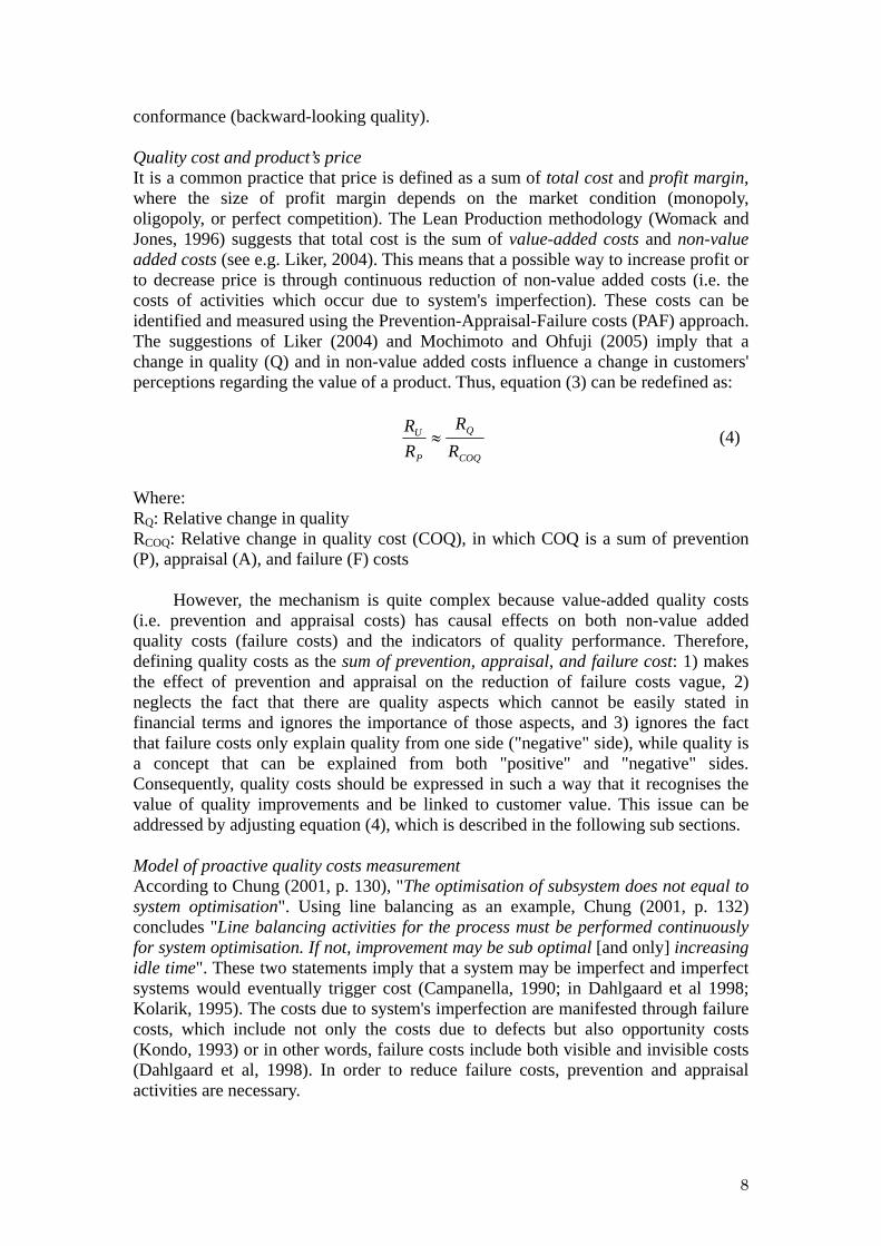
conformance (backward-looking quality). Quality cost and product’s price It is a common practice that price is defined as a sum of total cost and profit margin, where the size of profit margin depends on the market condition (monopoly, oligopoly, or perfect competition). The Lean Production methodology (Womack and Jones, 1996) suggests that total cost is the sum of value-added costs and non-value added costs (see e.g. Liker, 2004). This means that a possible way to increase profit or to decrease price is through continuous reduction of non-value added costs (i.e. the costs of activities which occur due to system's imperfection). These costs can be identified and measured using the Prevention-Appraisal-Failure costs (PAF) approach. The suggestions of Liker (2004) and Mochimoto and Ohfuji (2005) imply that a change in quality (Q) and in non-value added costs influence a change in customers' perceptions regarding the value of a product. Thus, equation (3) can be redefined as:

COQ

Q

P

U

RR

RR

≈ (4)

Where: RQ: Relative change in quality RCOQ: Relative change in quality cost (COQ), in which COQ is a sum of prevention (P), appraisal (A), and failure (F) costs

However, the mechanism is quite complex because value-added quality costs (i.e. prevention and appraisal costs) has causal effects on both non-value added quality costs (failure costs) and the indicators of quality performance. Therefore, defining quality costs as the sum of prevention, appraisal, and failure cost: 1) makes the effect of prevention and appraisal on the reduction of failure costs vague, 2) neglects the fact that there are quality aspects which cannot be easily stated in financial terms and ignores the importance of those aspects, and 3) ignores the fact that failure costs only explain quality from one side ("negative" side), while quality is a concept that can be explained from both "positive" and "negative" sides. Consequently, quality costs should be expressed in such a way that it recognises the value of quality improvements and be linked to customer value. This issue can be addressed by adjusting equation (4), which is described in the following sub sections. Model of proactive quality costs measurement According to Chung (2001, p. 130), "The optimisation of subsystem does not equal to system optimisation". Using line balancing as an example, Chung (2001, p. 132) concludes "Line balancing activities for the process must be performed continuously for system optimisation. If not, improvement may be sub optimal [and only] increasing idle time". These two statements imply that a system may be imperfect and imperfect systems would eventually trigger cost (Campanella, 1990; in Dahlgaard et al 1998; Kolarik, 1995). The costs due to system's imperfection are manifested through failure costs, which include not only the costs due to defects but also opportunity costs (Kondo, 1993) or in other words, failure costs include both visible and invisible costs (Dahlgaard et al, 1998). In order to reduce failure costs, prevention and appraisal activities are necessary.

8

Chung (2001, p. 127) further states that "... the efforts of improving quality [through prevention and appraisal activities] bring not only reducing the failure costs but also many other benefits which are tangible or intangible". This statement implies that the effects of quality improvements do not merely manifest into a change in failure costs but also other benefit-related quality performance results.

Kondo (1993) describes that increased quality performance (Q) will decrease

failure costs (F), and at the same time argues that the efforts to improve quality can be performed creatively, meaning that the same or higher level of quality performance can be achieved with lower prevention and appraisal (PA) costs (figure 1).

<Take in figure 1>

Figure 1. Creative quality improvements

Based on the thoughts of Kondo (1993) and Chung (2001), we conclude that: A discussion about quality improvement should include PA (the effort), an

indicator that explains quality-construct from the "positive" side (in this case, it is simply defined as Q), and an indicator that explains quality-construct from the "negative" side, i.e. the failure costs (F).

The prevention-appraisal activities (PA) have a direct effect on quality performance (Q) and subsequently affect the failure costs (F) because changes in quality performance will influence changes in failure costs.

Using these two points, a general model of the value of quality improvements will be constructed. After the suggested general model, two specific models of the value of quality improvements are suggested. General model of the value of quality improvements From the producer's perspective, assessing quality improvements is [essentially] a comparison between the benefits (i.e. changes in quality (Q) and failure costs (F)) gained from the improvements and the expenses to perform prevention and appraisal activities (PA). As a part of the job description of quality staffs or workers, it wouldn't be easy to point out whether a performed task is either P or A [because it might be a combination]. This became the motivation not to separate P and A. Treating P and A as a synergy may (depending on industry characteristics and the level of quality advancement in a company) provide a better explanation regarding the relationship between the efforts and the results of quality improvements. The ratio between the benefits of improvement and the expenses is defined as the value of quality improvements considering that value is a ratio between benefits and costs. Hence, the value of improvement may be expressed as a two-dimensional vector (v):

yRRx

RR

vPA

F

PA

Q ))⎟⎟⎠

⎞⎜⎜⎝

⎛+⎟⎟

⎠

⎞⎜⎜⎝

⎛= (5)

Where: RPA : The relative change in prevention and appraisal related expenses RQ : The relative change in quality performance results

9

RF : The relative change in failure costs yx )), : The directions (coordinates) of the value vector

The change in quality (Q) will likely influence customers' perceptions regarding

the benefits of the product, while the change in failure costs (F) will likely influence customers' perception regarding the sacrifices to acquire the product. The changes in the prevention-appraisal costs (PA) and failure costs (F) are usually measured in terms of money (e.g. $, £), and the change in quality performance (Q) is measured in terms of percentage (0-100%). These are the absolute measurements of PA, Q, and F, which are expressed in terms of differences (Δ) and take zero (0) as a reference point. However, it is also possible to measure the changes of PA, Q, and F in relative terms (R), where one (1) is the reference point. These alternative types of measurement are not contradictive − we just used different measurement scales. In this paper, the change of PA, Q, and F are measured in relative terms.

The analytical model (5) suggests that changes in prevention and appraisal

activities affect both the benefits from the changes in failure costs and quality performance. The former part of the equation (RQ/RPA) indicates the direct effect of improvement efforts, while the latter part of the equation (RF/RPA) indicates the subsequent effect of improvement efforts (meaning that the quality performance must be improved first before the failure cost can be reduced). Although the model does not accommodate the time lag of performance improvements, the value measurements indicate whether the overall relative benefits achieved through improvements are higher than the relative expenses to perform the improvement activities.

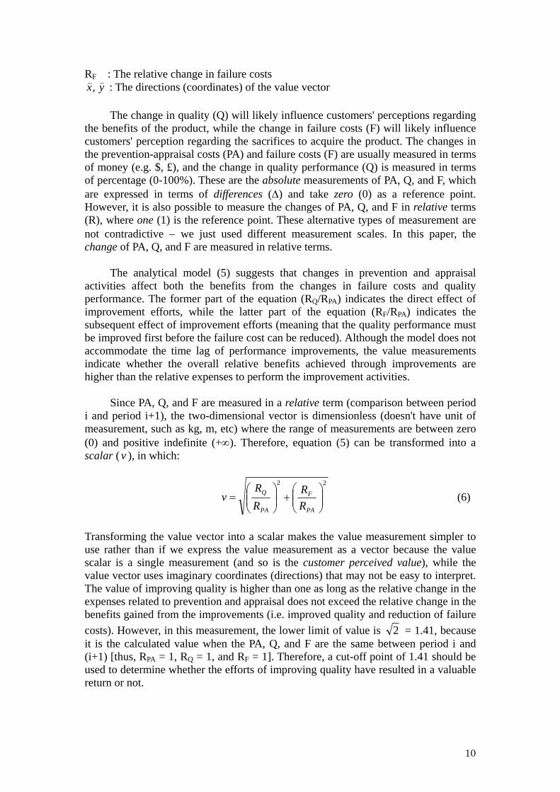
Since PA, Q, and F are measured in a relative term (comparison between period

i and period i+1), the two-dimensional vector is dimensionless (doesn't have unit of measurement, such as kg, m, etc) where the range of measurements are between zero (0) and positive indefinite (+∞). Therefore, equation (5) can be transformed into a scalar ( ), in which: v

22

⎟⎟⎠

⎞⎜⎜⎝

⎛+⎟⎟

⎠

⎞⎜⎜⎝

⎛=

PA

F

PA

Q

RR

RR

v (6)

Transforming the value vector into a scalar makes the value measurement simpler to use rather than if we express the value measurement as a vector because the value scalar is a single measurement (and so is the customer perceived value), while the value vector uses imaginary coordinates (directions) that may not be easy to interpret. The value of improving quality is higher than one as long as the relative change in the expenses related to prevention and appraisal does not exceed the relative change in the benefits gained from the improvements (i.e. improved quality and reduction of failure costs). However, in this measurement, the lower limit of value is 2 = 1.41, because it is the calculated value when the PA, Q, and F are the same between period i and (i+1) [thus, RPA = 1, RQ = 1, and RF = 1]. Therefore, a cut-off point of 1.41 should be used to determine whether the efforts of improving quality have resulted in a valuable return or not.

10

Specific models of the value measure Model 1: the value of improving forward-looking quality The benefit that the producer expects from the performed quality improvements is that the customers' perceptions regarding the quality of the product will be increased. Thus, customers' judgment on quality (Q(1)) is the indicator of forward-looking quality. The value of improving forward-looking quality (ν1) is therefore:

22

)1(1 ⎟⎟

⎠

⎞⎜⎜⎝

⎛+⎟⎟

⎠

⎞⎜⎜⎝

⎛=

PA

EF

PA

Q

RR

RR

v (7)

Where: RPA : The relative change in prevention and appraisal related expenses RQ(1) : The relative change in customers' judgment on quality REF : The relative change in external failure costs The change in prevention-appraisal costs (PA) is defined as the ratio between PA at period (i+1) and PA at period i. Then:

i

iPA PA

PAR 1+= (8)

If PA at period (i+1) is lower than the PA at period (i), the RPA is smaller than one. The change in failure costs is defined as the ratio between the external failure costs (EF) at period i and the external failure costs at period (i+1). Then:

1+

=i

iEF EF

EFR (9)

If the external failure costs (EF) at period (i+1) is lower than the failure costs at period (i), the REF is higher than one. We define RQ(1) as the ratio between the overall customer's cognitive judgment on quality (CCJQ) on period (i+1) and (i). Therefore:

i

iQ CCJQ

CCJQR 1

)1(+= (10)

It follows that RQ(1) is larger than one if the CCJQ is improved from period (i) to period (i+1). Considering the practicality aspect, Q(1) may be measured e.g. every six months or annually. If we first measure it at month 1 (i.e. period i) then the next measurement is at month 7 (i.e. period (i+1)). The measurement of ν1 in (7) requires that the "distance" between period (i) and period (i+1) of RQ1 should be equal to the "distance" between period (i) and period (i+1) of REF and RPA. CCJQ is a measure of customers’ perceptions regarding the quality of a company's product or service. There are two ways of measuring CCJQ: single-attribute (overall)

11

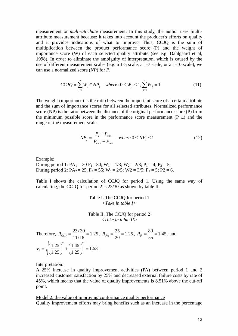
measurement or multi-attribute measurement. In this study, the author uses multi-attribute measurement because: it takes into account the producer's efforts on quality and it provides indications of what to improve. Thus, CCJQ is the sum of multiplication between the product performance score (P) and the weight of importance score (W) of each selected quality attribute (see e.g. Dahlgaard et al, 1998). In order to eliminate the ambiguity of interpretation, which is caused by the use of different measurement scales (e.g. a 1-5 scale, a 1-7 scale, or a 1-10 scale), we can use a normalized score (NP) for P.

(11) ∑∑==

=≤≤=n

jjj

n

jjj WWwhereNPWCCJQ

11

1,10:*

The weight (importance) is the ratio between the important score of a certain attribute and the sum of importance scores for all selected attributes. Normalized performance score (NP) is the ratio between the distance of the original performance score (P) from the minimum possible score in the performance score measurement (Pmin) and the range of the measurement scale.

10minmax

min ≤≤−

−= j

jj NPwhere

PPPP

NP (12)

Example: During period 1: PA1 = 20 F1= 80; W1 = 1/3; W2 = 2/3; P1 = 4; P2 = 5. During period 2: PA2 = 25, F2 = 55; W1 = 2/5; W2 = 3/5; P1 = 5; P2 = 6. Table I shows the calculation of CCJQ for period 1. Using the same way of calculating, the CCJQ for period 2 is 23/30 as shown by table II.

Table I. The CCJQ for period 1 <Take in table I>

Table II. The CCJQ for period 2

<Take in table II>

Therefore, 25.118/1130/23

)1( ==QR , 25.12025

==PAR , 45.15580

==FR , and

53.125.145.1

25.125.1 22

1 =⎟⎠⎞

⎜⎝⎛+⎟

⎠⎞

⎜⎝⎛=v .

Interpretation: A 25% increase in quality improvement activities (PA) between period 1 and 2 increased customer satisfaction by 25% and decreased external failure costs by rate of 45%, which means that the value of quality improvements is 8.51% above the cut-off point.

Model 2: the value of improving conformance quality performance Quality improvement efforts may bring benefits such as an increase in the percentage

12

of the produced products that conforms to specifications or backward-looking quality (Q(2)). Therefore, the value of improving backward quality (ν2) is defined as:

22

)2(2 ⎟⎟

⎠

⎞⎜⎜⎝

⎛+⎟⎟

⎠

⎞⎜⎜⎝

⎛=

PA

IF

PA

Q

RR

RR

v (13)

We may define:

i

iQ Y

YR 1

)2(+= (14)

Where: Yi+1: The yield (the percentage of conforming products) at period (i+1) Yi: The yield at period i

It follows that RQ(2) is greater than one if the yield at period (i+1) is larger than the yield at period (i). While RPA follows the definitions as shown by equation (8), and the relative change in internal failure cost (RIF) is measured in a similar way as equation (9). Even though there are additional factors, which might influence yield, yield has been used as an indicator of conformance quality.

Considering the practicality aspect, Q(2) may be measured e.g. every month or quarterly, while Q(1) may be measured e.g. every six months or annually. This means that the "distance" between period (i) and period (i+1) for Q(1) and Q(2) may not be equally long, but the "distance" between period (i) and period (i+1) of RQ(2) should be equal to the "distance" between period (i) and period (i+1) of RPA and RIF. In the case Q(2) is measured quarterly, if we first measure it at month 1 (i.e. period i) then the next measurement is at month 4 (i.e. period (i+1)).

Example: Let's assume that: During period 1: Y1 = 0.8; PA1 = 30, F1 = 70, and during period 2: Y2 = 0.9; PA2 = 30, F2 = 60. Then we get = 0.9/0.8 = 1.12, R)2(QR PA = 1, RIF = 70/60 = 1.17, and

62.1117.1

112.1 22

2 =⎟⎠⎞

⎜⎝⎛+⎟

⎠⎞

⎜⎝⎛=v .

The result can be interpreted in the following way: The same amount of efforts to improve quality (but more creatively) increased the yield by 12.5% and decreased the internal failure costs by a rate of 17%. Thus, the value of quality improvements is 14.89% above the cut-off point.

Case study The case company described in this paper is a Swedish wood-flooring manufacturer, and one of Europe's leading parquet and wood-flooring producers that mainly serves US and European markets. The average sales revenue during 2003-2004 was more than 200 millions Euros per year.

13

Selecting the model to be applied Based on the general model of proactive quality cost (equation (6)), there are two specific models to be applied, i.e. equation (7) and (13). However, considering the company’s priority to first improve quality in the production (where quality cost measurements become the indicator), the case study only demonstrates the applicability of the second specific model of the value of quality improvements (i.e. equation (13)). Another consideration to first apply equation (13) is the emphasis on the necessity of being customer value-oriented when measuring quality cost although those measurements contain data that are identified backward in the production. In this paper, we analysed ten (10) sets of data that have been collected in the case company. Model validation The data analysis (see figure 2) indicates that quality improvement efforts do have effects on the quality improvement indicators (R2 = 94.61%), which supports our reasoning to adjust equation (4) into equation (5) and also validates equation (13). Figure 2 explains the concept of creative quality improvements in the following way:

• Higher results (from y ≈ 1.34 to y ≈ 1.54) can be achieved with the same amount of efforts (x ≈ 0.96)

• The same results (y ≈ 1.40) can be achieved with less amount of efforts (from x ≈ 1.33 to x ≈ 0.82)

<Take in figure 2>

Figure 2. The effect of quality improvement efforts on quality improvement indicators The two “extreme” points, one on the right (RPA ≈ 1.70) and one on the left hand side (RPA ≈ 0.56) have been ignored in the above explanation because they may be regarded as outliers until more data have been collected. When more data are collected around the extreme values of RPA, the function in figure 2 is likely to change and may then be used as a tool for prediction. Until now, the estimated function in figure 2 was only used to show potential effects of creative quality improvement efforts. The operating definition of Q(2) The yield (stated as a fraction of total output) of thick wood-flooring products (15 mm) are defined as the quality indicator (Q(2)), where these data are collected at the final inspection (after profiling process) before the products are packed and delivered to the distribution centre. Quality cost identification and measurements With reference to equation (4) that has been adjusted into equations (5) and (6), the Prevention-Appraisal-Failure (PAF) model according to British Standard (BS) 6143 was selected to identify the quality cost in the case company because it provides a standardization regarding quality cost. Although the PAF model (and BS 6143) has been put under scrutiny and constructively criticized for a number of reasons (Dahlgaard et al, 1992; Dale and Plunkett, 1999), it does make users aware that failures cause reduced profits and change (i.e. reduction of failures) will improve overall performance and quality (Keogh et al, 1998). Also manufacturing industries mostly implement the PAF model (Keogh et al, 2003) since it is easy to understand

14

and is universally accepted (Dale and Plunkett, 1999), and the method of categorizing quality cost is the most common method in literature (Chiadamrong, 2003). Using a standardized model is beneficial because identifying quality costs requires a “careful” definition of what quality-related costs are because it is not easy to disown a cost element after being claimed as quality-related, i.e. the danger of potential backfire of amplifying quality cost (Dale and Plunkett, 1999).

The quality cost identification project was intended as the foundation or the starting point for continuous quality improvement by showing the activities or events that drive quality cost and state them in terms of financial figures. Simplicity and the use of existing data are among the keywords of how quality cost was identified and visualized in the company. Simplicity in this case means that quality cost identification was mostly focused on the cost elements that were "easy to capture" as well as the use of simple mathematical equations to express them. Mathematical equations were used to estimate the costs that are not recorded in the company's accounting/financial system.

A systematic collection of quality costs was suggested to consist of the following serial process: define, streamline, identify, and allocate. Define means "translate" the definition of quality cost elements into the specific industrial context, in this case a wood-flooring manufacturer. Streamlining means to consider the quality cost elements that are applicable to a significant extent in the company. The next step is to identify the cost drivers of the quality cost elements. These three steps were performed as a qualitative study through interviews, brainstorming, and observations. The use of qualitative studies in quality cost identification is common, especially interviews (see e.g. Suresh et al (2000), Keogh et al (2003)).

The last step, allocate, is concerned with the process of allocating costs using bases such as: number of inspections, percentage of total working time (or duration) to perform a certain activity, number of complaints, number of defects, volume of scraps. This process is the quantitative study of quality cost identification, where mathematical algorithms were developed for the purpose of allocation. Figure 3 describes the systematic way of collecting, measuring, and reporting quality costs.

<Take in figure 3>

Figure 3. Systematic collection, measurement, and reporting quality costs Quality cost reporting is done regularly every month, every quarter, and every year in order to assess the progress of quality improvements.

The system to identify and document quality cost consists of four parts: 1) a file

that contains the definition of quality cost elements in the industry/company context, 2) a file that contains mathematical algorithms to describe the way of calculating the costs, 3) a spreadsheet-based cost calculation, and 4) a file used for quality cost reporting. The quality cost results reported first time by using this system are shown in table III.

Table III. Quality cost results during 2004

<Take in table III>

15

The internal failure cost is the largest portion of the quality cost measurements and prevention cost is the smallest cost category. The combination of internal and external failure cost is higher than prevention and appraisal. These results are consistent with the characteristics of quality cost as described in the theory section. The figures in table III indicate that the quality activities in the company are managed in a reactive way instead of a preventive way.

The value of quality improvements The relative change in quality (RQ(2)) is calculated according to equation (14), and is shown in table IV.

Table IV. Relative changes in quality <Take in table IV>

The relative change in prevention-appraisal costs (PA) and internal failure costs (IF) is shown in table V.

Table V. Relative changes in PA and IF <Take in table V>

The value of improving the conformance quality was estimated using equation (13). However, as discussed above, the calculated value measurements are sensitive to "extreme" changes of its variables and because of that, it is not always easy to "extract" a meaningful interpretation from a fluctuating figure. This problem may be overcome by smoothing the results using Exponentially Weighted Moving Average (EWMA) method (see e.g. Wadsworth, 2000). By using this method, fluctuations are reduced and shifts can be detected, which facilitate interpretation of the results. Table VI shows the value of improving backward quality (ν2) and the EWMA of ν2, where the initial value of EWMA (ν2) is set at 90% of ν2 during Jan-Feb and the smoothing factor is 0.1, which is one of the most commonly used smoothing factors (Wadsworth, 2000). The result is plotted in figure 4.

Table VI. The value of improving the conformance quality <Take in table VI>

<Take in figure 4>

Figure 4. The value of quality improvements If we take v = 1.41 as a cut-off point, figure 4 indicates that between January and June, the value of improving the conformance quality was below the cut-off point (although it is increasing), while between July to November, the value of improving conformance quality was above the cut-off point. Thus, the quality improvement efforts during the last six months fulfil the expectations, meaning that benefits were higher than the expenses. Discussion In this article, relative measurements of value were used which enabled us to combine different types of measurement scales and the transformation of the value vector into a scalar simplifying the value measurement.

16

The way customers perceive the value of a product is a function of the value of quality improvements, where it is assumed that the function is positive and increasing, meaning that when the value of quality improvements goes up, the relative change in perceived customer value also goes up. This implies that valuable quality improvements are the means to influence the perceived customer value of a product, and the dynamics of customer value is the result of continuous improvement efforts to increase the quality of a product and/or decreasing the costs due to non-conformance.

The changes in prevention-appraisal costs, failure costs, and yield are the determining variables whether the improvements have given more than fair return (ν>1.41), relatively fair return (ν ≈1.41), or less than fair return (ν<1.41). In other words, the value of quality improvements indicates the return on quality improvement (ROQI), which measures the return on the “investments” (in terms of employees’ efforts and knowledge as well as other resources) to reach a higher level of quality performance. It might be important to note that when ν<1.41, it should not be interpreted as an indication of failure in quality improvement. Instead, it may indicate that the efforts of improving quality could have been performed smarter in order to have a stronger effect on the value to both producer and customers. Conclusions The weakness of the existing concept of quality costs is obvious when we reflect on the fundamental purpose of quality management, i.e. creating customer satisfaction and value. Hence, measuring quality performance should not just involve costs viewed from producer's perspective, but it should also be about measuring quality performance in terms of value seen from customers' perspective.

Understanding and improving quality cost in a value-context is to think

proactively, because quality cost measurements: 1) can be used to assess whether the improvement activities were valuable (gave more benefits compared to the expenses), and 2) can lead to an understanding that the efforts of improving product and process quality, also influence the way customers perceive the value of the product.

This paper has described a new method for measuring quality costs (define,

streamline, identify, and allocate) and transforming the measurements into value of quality improvements (ROQI). The value measure (ROQI) indicates that quality improvement efforts are valuable (give more than fair return) if the gained overall benefits (the increase of a quality indicator, e.g. yield, and the decrease of failure costs) are higher than the costs to perform improvement activities, or if the same or higher benefits can be gained at the same or lower expenses.

The method has been theoretically developed and tested in a Swedish wood

flooring manufacturer. More empirical tests are needed to give further insights regarding practical implementation problems in other industries. References Angell, L.C., Chandra, M.J. (2001), "Performance implications of investments in

continuous improvement", International Journal of Operations & Production Management, Vol. 21, No. 1/2, pp. 108-125.

17

Bounds, G., Yorks, L., Adams, M., Ranney, G. (1994), Beyond Total Quality Management: toward the emerging paradigm, McGraw-Hill, New York.

Breyfogle, F.W., Cupello, J.M., Meadows, B. (2001), Managing Six Sigma, John Wiley & Sons, Inc., Canada.

Chen, L.H., Weng, M.C. (2002), "Using fuzzy approaches to evaluate quality improvement alternative based on quality costs", International Journal of Quality & Reliability Management, Vol. 19, No. 2, pp. 122-136.

Chiadamrong, N. (2003), "The development of an economic quality cost model", Journal of Total Quality Management & Business Excellence, Vol. 14, No. 9, pp. 999-1014.

Chung, K.S. (2001), "Rethinking for the monetary effect of quality improvement activities", Proceedings of The Sino-Korea International Conference on Quality Science and Productivity Promotion, Zhengzhou, China.

Conti, T. (1993), Building total quality: a guide for management, Chapman & Hall. Conti, T. (2005), "Quality and Value: Convergence of Quality Management and

System Thinking", in the Proceeding of World Conference on Quality and Improvement, Seattle.

Dahlgaard, J.J., Kristensen, K., Kanji, G.K. (1992), "Quality costs and total quality management", Total Quality Management, Vol. 3, No. 3, pp. 211-221.

Dahlgaard, J.J., Kristensen, K., Kanji, G.K. (1998), Fundamentals of total quality management, Nelson Thornes, UK.

Dale, B.G., Plunkett, J.J. (1999), Quality Costing, 3rd edition, Chapman & Hall. Dumond, E.J (2000), "Value Management: an underlying framework", International

Journal of Operations & Production Management, Vol. 20, No. 9, pp. 1062-1077. Feigenbaum, A.V. (1956), "Total Quality Control", Harvard Business Review, Vol.

34, No. 6, pp. 93-101. Feigenbaum, A.V. (1991), Total Quality Control, 3rd edition, McGraw-Hill. Gale, B.T. (1994), Managing Customer Value, The Free Press, New York. Juran, J.M (1951), Quality Control Handbook, McGraw Hill Book Company, Inc.,

New York. Juran, J.M. (1998), Juran's Quality Handbook, 5th edition, McGraw-Hill. Keogh, W., Atkins, M.H., Dalrymple, J.F. (1998), "Human resource issues in quality

cost: results from a longitudinal study", Total Quality Management, Vol. 9, No. 4&5, pp. 141-144.

Keogh, W., Dalrymple, J.F., Atkins, M.H. (2003), "Improving performance: quality costs with a new name?", Managerial Auditing Journal, 18/4, pp. 340-346.

Khalifa, A. S. (2004), "Customer value: a review of recent literature and an integrative configuration", Journal of Management Decision, Vol. 42, No. 5, pp. 645-666.

Kolarik, W.J. (1995), Creating Quality: concepts, systems, strategies, and tools, McGraw-Hill

Kondo, Y. (1993), Companywide Quality Control, 3A Corporation, Tokyo-Japan. Liker, J.K. (2004), The Toyota Way, McGraw-Hill, New York. Mandal, P., Shah, K. (2002), "An analysis of quality costs in Australian

manufacturing firms", Total Quality Management, Vol. 13, No. 2, pp. 175-182. Millar, I. (1999), "Performance improvement. Part 2", Industrial Management & Data

System, 99/6, pp. 257-265. Mochimoto, T., Ohfuji, T. (2005), "A Study on Quality Corresponding to Price", in

JUSE (Ed), Quality Evolution - Way to Sustainable Growth, Proceeding of International Conference on Quality, Tokyo-Japan, II-5, pp. 1-12.

18

Moen, R.M. (1998), New quality cost model used as top management tool, The TQM Magazine, Vol. 10, No. 5, pp.334-341.

Omachonu, V.K., Suthummanon, S., Einspruch, N.G. (2004), The relationship between quality and quality cost for a manufacturing company, International Journal of Quality & Reliability Management, Vol. 21, No. 3, pp. 277-290.

Padula, G., Busacca, B. (2005), "The asymmetric impact of price-attribute performance on overall price evaluation", International Journal of Service Industry Management, Vol. 16, No. 1, pp. 28-54.

Prickett, T.W., Rapley, C.W. (2001), Quality Costing: a study of manufacturing organisations. part2: main survey, Journal of Total Quality Management, Vol. 12, No. 2, pp. 211-222.

Roden, S., Dale, B.G. (2000), Understanding the language of quality costing, The TQM Magazine, Vol. 12, No. 3, pp. 179-185.

Sandoval-Chavez, D.A., Beruvides, M.G. (1998), Using opportunity costs to determine the cost of quality: a case study in a continuous-process industry, The Engineering Economists, Vol. 43, No. 2, pp. 107-124.

Setijono, D., Dahlgaard, J.J. (2007), "Customer value as a key performance indicator (KPI) and a key improvement indicator (KII)", Measuring Business Excellence, Vol. 11, No. 2, pp. 44-61.

Shah, K.K.R, Fitzroy, P.T. (1998), "A review of quality cost surveys", Total Quality Management, Vol. 9, No. 6, pp. 479-486.

Suresh, K.K., Arawati, A., Nooreha, H. (2000), "Cost of quality: the hidden cost", Total Quality Management, Vol. 11, No. 4/5&6, pp. 844-848.

Tsai, W.H. (1998), "Quality Cost Measurement Under Activity-Based Costing", International Journal of Quality & Reliability Management, Vol. 15, No. 7, pp. 719-752.

Williams, A.R.T., van der Wiele, A., Dale, B.G. (1999), "Quality costing: a management review", International Journal of Management Reviews, Vol. 1, Issue 4, pp. 441-460.

Womack, J.P., Jones, D.T. (1996), Lean Thinking: Banish Waste and Create Wealth in Your Corporation, Simon & Schuster, New York.

Woodsworth, H.M. (2000), "Statistical Process Control", in Juran, J.M., Godfrey, A.B. (Eds), Juran's Quality Handbook, 5th edition, McGraw Hill.

Zeithaml, V.A. (1988), “Consumer perception on price, quality, and value: a means-end model and synthesis of evidence”, Journal of Marketing, Vol. 13, No. 2, pp. 314-332.

19

LIST OF FIGURES

Figure 1

Quality of conformance

Cost

Q2

Failure costsPrevention + Appraisal

costs

Q1

Figure 2

y = 4,4178x4 - 23,135x3 + 44,04x2 - 36,368x + 12,442R2 = 0,9461

0

0,5

1

1,5

2

2,5

0 0,5 1 1,5 2

PAR

22)2( IFQ RR +

20

Figure 3

BS 6143 DefineStream-

lineIdentify Allocate

Industry context

Result

Company activities

Cost drivers

Algorithms

Qualitative study Quantitative study

Figure 4

0

0,2

0,4

0,6

0,8

1

1,2

1,4

1,6

1,8

jan-fe

b

feb-m

ar

mar-ap

r

apr-m

ay

may-ju

njun

-jul

jul-aug

aug-s

ep

sep-o

ct

oct-n

ov

v

21

LIST OF TABLES Table I Attribute W NP W*NP

1 1/3 (4-1)/(7-1) = 1/2 1/6 2 2/3 (5-1)/(7-1) = 2/3 4/9

Total 1 CCJQ = 11/18 Table II Attribute W NP W*NP

1 2/5 (5-1)/(7-1) = 4/6 8/30 2 3/5 (6-1)/(7-1) = 5/6 15/30

Total 1 CCJQ = 23/30 Table III

Category Portion Percent of sales Prevention 2.5% < 1% Appraisal 15.5% < 1%

Internal failure 53% 1-2 % External failure 29% 1-2 %

Total 100% 3-4 % Table IV

RQ(2)Jan-Feb 0.9997 Feb-Mar 0.9996 Mar-Apr 0.9977 Apr-May 0.9973 May-Jun 1.0064 Jun-Jul 0.9958 Jul-Aug 0.9988

Aug-Sept 1.0092 Sept-Oct 0.9998 Oct-Nov 1.0022

Table V

RPA RIFJan-Feb 0.9556 0.8993 Feb-Mar 1.3294 0.9860 Mar-Apr 0.8194 0.9555 Apr-May 0.9439 1.0733 May-June 0.9563 1.1730

Jun-Jul 0.5640 2.1274 Jul-Aug 1.6995 0.5172

Aug-Sept 1.1190 0.8759 Sept-Oct 1.0699 0.8539 Oct-Nov 0.9796 1.0471

22

Table VI ν2 EWMA (ν2)

Jan-Feb 1.4072 1.2665 Feb-Mar 1.0562 1.2455 Mar-Apr 1.6859 1.2895 Apr-May 1.5521 1.3158 May-June 1.6161 1.3458

Jun-Jul 4.3022 1.6414 Jul-Aug 0.6618 1.5435

Aug-Sept 1.1942 1.5086 Sept-Oct 1.2230 1.4800 Oct-Nov 1.4866 1.4807

23