Tomographic SAR

Gianfranco Fornaro National Research Council (CNR)

Institute for Electromagnetic Sensing of the Environment (IREA) Via Diocleziano, 328

I-80124 Napoli ITALY

fornaro.g@irea.cnr.it

ABSTRACT Synthetic Aperture Radar (SAR) tomography is a technique that has been intensely developed in the last years for the analysis of complex scenarios. SAR Tomography is based on the principle of synthesizing a large aperture along the height provide imaging radar 3D resolution capabilities. SAR tomography can be applied to the imaging of scattering distributed along the vertical direction such as forest mapping with lower frequency (L and P-Band) SAR systems; with higher frequency (C and X-Band) sensors, where penetration is very limited and the scattering mainly occurs at the surface level SAR tomography allows tackling problems that limits classical SAR Interferometry related to the interference of scatterers within the same pixels due to the occurrence of layover. This paper aims to provide an overview of the technique by explaining the basics concepts of SAR tomography and illustrating the advantages over classical SAR interferometry. Results achieved by processing real spaceborne data are provided to show the capabilities and potentialities of the application of SAR tomography.

1.0 INTRODUCTION

Synthetic Aperture Radar (SAR) systems exploit the possibility to synthesize a large antenna along the azimuth direction to achieve a sharp beam that allows reaching resolutions up to the order of 1m. This option is possible thank to the capability to transmit a coherent radiation, i.e. with regular oscillations. SAR focusing is the operation that allows the azimuth beam sharpening and therefore the generation of high resolution 2D images of the backscattered radiation [1]. The reality is 3D and the resulting image represents only an integration along the elevation direction, also referred to as normal-to-slant-range direction, of the 3D scene scattering properties onto the 2D azimuth-range plane.

Assuming that the radiation penetration is negligible and that the mapping from 3D to the 2D (azimuth-range plane) is injective SAR Interferometry (InSAR) is a technique that, by exploiting at least two antennas which image the scene from slightly different look angles, is able to provide the reconstruction of the 3D scattering properties and hence the scene topography (Digital Elevation Model). Key point of this technique is the determination of the off-nadir angle, on a pixel-by-pixel basis, of the effective phase centre of the scatterers within the resolution cell. This information, in addition to the knowledge of the azimuth and range pixel coordinates provided by the SAR focusing operation, allows the complete localization of the (mean or dominant) scattering mechanism and therefore the reconstruction of the height scene profile [1][2]. Differential Interferometry (DInSAR), is a further advance of InSAR for the detection and mapping of ground deformations which has considerably increased the use of SAR data in geophysics, hydrology and in general for civilian and surveillance applications [3].

Either due to the intrinsic side-looking characteristic of the imaging system (which discriminate distances and hence is affected by layover) or to the penetration of the radiation below the surface mapping from 3D to the 2D (azimuth-range) domain can be surjective. Hence target characterization and localization cannot be carried out neither by two measurements (i.e. by a single baseline) nor via classical interferometric approaches.

STO-EN-SET-191-2014 8 - 1

Tomographic SAR

The recent advances of the space technology involving constellations of satellites, and the planning for future missions involving formation of satellites able to acquire simultaneous (multi-baseline) SAR images repeatedly over the time, have pushed the research in the development of new techniques capable of processing, jointly and coherently, stacks of SAR images. Available archives are filled with datasets acquired over the same scene at different times and with varying imaging geometries (spatial baselines).

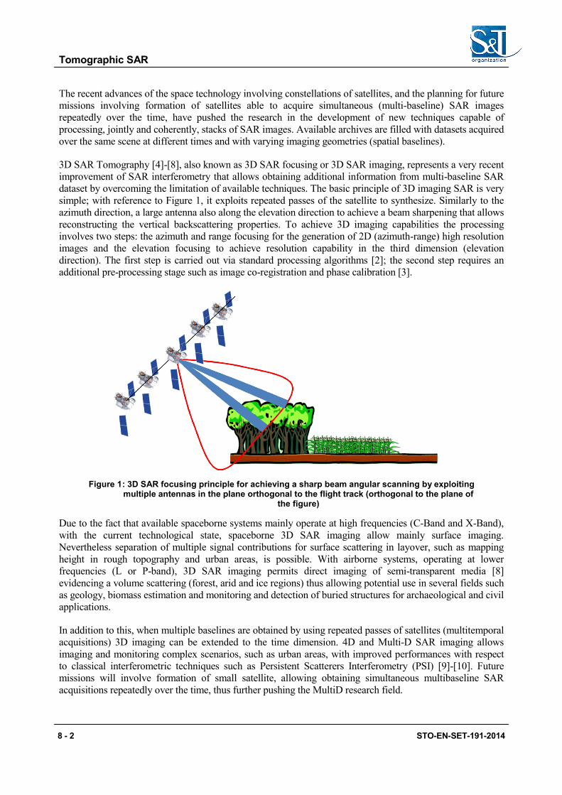
3D SAR Tomography [4]-[8], also known as 3D SAR focusing or 3D SAR imaging, represents a very recent improvement of SAR interferometry that allows obtaining additional information from multi-baseline SAR dataset by overcoming the limitation of available techniques. The basic principle of 3D imaging SAR is very simple; with reference to Figure 1, it exploits repeated passes of the satellite to synthesize. Similarly to the azimuth direction, a large antenna also along the elevation direction to achieve a beam sharpening that allows reconstructing the vertical backscattering properties. To achieve 3D imaging capabilities the processing involves two steps: the azimuth and range focusing for the generation of 2D (azimuth-range) high resolution images and the elevation focusing to achieve resolution capability in the third dimension (elevation direction). The first step is carried out via standard processing algorithms [2]; the second step requires an additional pre-processing stage such as image co-registration and phase calibration [3].

Figure 1 : 3D SAR focusing principle for achieving a sharp beam angular scanning by exploiting multiple antennas in the plane orthogonal to the flight track (orthogonal to the plane of

the figure)

Due to the fact that available spaceborne systems mainly operate at high frequencies (C-Band and X-Band), with the current technological state, spaceborne 3D SAR imaging allow mainly surface imaging. Nevertheless separation of multiple signal contributions for surface scattering in layover, such as mapping height in rough topography and urban areas, is possible. With airborne systems, operating at lower frequencies (L or P-band), 3D SAR imaging permits direct imaging of semi-transparent media [8] evidencing a volume scattering (forest, arid and ice regions) thus allowing potential use in several fields such as geology, biomass estimation and monitoring and detection of buried structures for archaeological and civil applications.

In addition to this, when multiple baselines are obtained by using repeated passes of satellites (multitemporal acquisitions) 3D imaging can be extended to the time dimension. 4D and Multi-D SAR imaging allows imaging and monitoring complex scenarios, such as urban areas, with improved performances with respect to classical interferometric techniques such as Persistent Scatterers Interferometry (PSI) [9]-[10]. Future missions will involve formation of small satellite, allowing obtaining simultaneous multibaseline SAR acquisitions repeatedly over the time, thus further pushing the MultiD research field.

8 - 2 STO-EN-SET-191-2014

Tomographic SAR

This paper aims to provide a discussion about the principles of SAR Tomography, to summarize the main achievements in terms of advanced processing algorithms such as 4D and MultiD SAR imaging and to show applications of the technique to simulated and real spaceborne data.

2.0 BASICS OF SAR TOMOGRAPHY

2.1 Geometry and models for 3D SAR imaging We refer to the geometry of the MP 3D-SAR system of Figure 1 where we consider the availabilities of N antennas (possibly implemented with repeat passes of a single antenna sensor) over the orbits S1,..., SN. characterized by spatial offsets that provide angular imaging diversity. A Cartesian reference system is adopted to describe the geometry: zrx ,, are the azimuth, range and height axes, respectively; s (orthogonal to the azimuth-range plane) is the elevation.

Figure 2 : 3D SAR focusing geometry

Under the Born weak-scattering approximation we have the following expression for the focused data the azimuth range sample ( )rx ′′, at the generic (n-th) antenna:

( ) ( ) ( ) ( )∫∫∫

−−′−′=′′

srxRj

nnsrxdsrrxxfdrdxrx

,,4

e ,,,,ˆ λπ

γγ (1)

where λ is the operating wavelength, ( )rsxRn ,, represents the distance of antenna n (n=1,…,N) from the generic point target, see Figure 2, ( )⋅γ is the function that models the 3D (volumetric) scene scattering properties and ( )⋅f is the (azimuth-range) point spread function (PSF). Equation (1) shows that the generic SAR image is the result of integration along the elevation direction that performs a mapping of 3D scene backscattering properties onto the azimuth - (slant) range plane.

STO-EN-SET-191-2014 8 - 3

Tomographic SAR

In 3D SAR imaging azimuth and range focusing as well as image registration is carried out as first processing stage. To simplify the notation in the following we assume the azimuth (Doppler) and range (transmitted) bandwidths are large enough to allow approximating the post focusing PSF with a 2D Dirac generalized function. Under these assumptions, for a given pixel ),( rx , the signal sample nh measured at the n-th antenna is given by:

( )

∫−

= dseshsRj

nnλ

π

γ4

)( (2)

and the integral is assumed to involve an interval with extension 2a (support of the scene along the elevation direction). A procedure, referred to as de-ramping compensation with respect to a reference point O, is at this stage applied to compensate for the phase quadratic distortion due to the Fresnel phase approximation, see Figure 3. This operation involves the following multiplication by the distance of the reference point (which is typically adapted on a pixel basis onto an available external DEM):

( ) ( ) ( )[ ]

∫∫ −−−−≈== dsesdsesehg sjRsRjRj

nnn

nnn πζλπ

λπ

γγ 20404

)()( , rbn

n λζ 2

= (3)

Figure 3 : Geometry relevant to the de-ramping procedure

where nb is the orthogonal baseline of the n-th antenna with respect to the master antenna. The last approximation is the result of an expansion of the difference ( ) ( )0nn RsR − and of the association of an inessential s2-dependent term in the unknown backscattering function. Equation (3) shows that the relation between the received signal (for n=1,…,N) and the unknown backscattering function is a Fourier series.

By collecting ng in a data vector g , by sampling )(sγ in ms (m=1,…,M) and by collecting the samples in a vector γ , the problem to reconstruct the unknown samples of )(sγ consists of inverting the following linear system:

8 - 4 STO-EN-SET-191-2014

Tomographic SAR

Aγg =

=−−

−−

MNN

M

sjsj

sjsj

ee

ee

πζπζ

πζπζ

22

22

1

111

, (4)

where A is a NxM matrix (model or sensing matrix) whose (N-dimensional) column vectors:

[ ] Mmee mNm sjsjm ,...1,....., 22T 1 == −− πζπζa , (5)

are referred to as steering vectors associated with the elevations ms (m=1,…,M), i.e. with the angle rsm / ( )2ar >> .

In general M is chosen at least equal to (typically larger than) N to preserve the spatial details of the reconstructed backscattering function contained in the measurements.

2.2 Inversion via beam-forming A very simple and robust inversion of (3) ((4) in the discrete case) can be carried by using the conjugate operator associated with the operator (hermitian, or transpose conjugate in the discrete case), i.e.:

gLγ H1ˆN

= (6)

that is:

gaH1ˆ mm N=γ (7)

for the backscattering at the elevation sample m (the scaling factor is introduced to preserve the power of the backscattering signal). The reconstruction algorithm is referred to as Beam-Forming (BF) [5][6] and has an equivalent interpretation in the framework of matched filtering.

To fully understand the rational of the above inversion method we refer to a simple case in which it is assumed that baselines are uniformly distributed with a baseline separation of b∆ : this case is also referred to Uniform Linear Array (ULA). The following condition:

arb

4λ

=∆ (8)

that is a spectral separation of

a2

1=∆ζ (9)

associated with a sampling of the spectrum of the function )(sγ to the Nyquist limit [11].

Letting N=M the matrix A assumes a Vandermonde structure [12]. Choosing a separation for the samples in s of:

STO-EN-SET-191-2014 8 - 5

Tomographic SAR

Nas 2

=∆ (10)

it results that:

NmeeNm

NjmNj

m ,...1,.....,22

T =

=

−−ππ

a (11)

In this conditions the matrix A becomes then a DFT matrix, that is (but for a proper scaling) a unitary matrix: the hermitian matrix in (6) becomes therefore an inverse matrix. According to the Nyquist sampling, the highest achievable resolution is given by the following Rayleigh limit:

Na

Brs 2

2==

λδ bNB ∆= (12)

where bNB ∆= is the total baseline span.

In the most general case, i.e. non uniform baselines sampling, the (in general non diagonal) MxM matrix AHA describes in Point Spread Function of the acquisition and (inversion by BF) imaging system along the elevation which is in general space variant. It is worth to point out that in the case M>N, AHA has a maximum rank of N, so that it cannot be in any case a diagonal matrix; accordingly the maximum spatial resolution is Na2 and can never reach the sampling step Ma2 ; moreover the reconstruction shows the presence of sidelobes which can reach, in the general case of uneven baseline distribution, also high levels.

3.0 ADVANCED 3D INVERSION METHODS

BF inversion described in the previous section is a simple, effective and robust technique that founds on the theory of matched filters. In this section, it is given a brief review of advanced 3D inversion algorithms, able to achieve either or both super-resolution improvements and sidelobes reduction.

3.1 Inversion via Singular Value Decomposition SVD is a tool that allows analysing the property of a matrix, or better of compact operator in the more general case of transformation of continuous signals, and implementing an effective regularized and “controlled”, inversion of linear problems. By applying the SVD analysis [12], the sensing matrix A is amenable of a representation in terms of a singular system { }N

nnnn 1,, =uvσ , where nσ are the eigenvalues of A, nv and nu are the orthonormal basis for the subspace of the visible objects (subspace normal to the null-space) and the orthonormal basis for the range of the operator A, respectively.

Introduction of the singular system allows writing the following two fundamental relations that connect the data space and the object (unknown) space [12]:

∑ ==

N

n nnn1Hγvug σ (13)

∑ ==

N

n nnn

1H1 guvγ

σ (14)

8 - 6 STO-EN-SET-191-2014

Tomographic SAR

Equations (13) and (14) represent the fundamental result of the SVD analysis: the first equation describes how the data is composed starting from the unknown γ . It states that all the different vectors ku concur, in principle, to the composition of the observed vector g : each contribution is however weighted by the associated singular value nσ thus leading to a strengthening or weakening of the mapping depending on the magnitude of the singular values.

Singular values are inverted in the inversion formula in (14). In a real case where data are corrupted by the noise, the presence of low singular values highlights the involvement of critical (weak) directions where the signal could be even overwhelmed by the noise. Accordingly, should not those directions be identified and properly handled with during the inversion process, high instabilities in the output reconstruction could be observed as a result of the noise amplification [13].

Low singular values are generally present in the presence of a non-uniform baseline distribution which causes an uneven distribution of the spectral samples, see (3). With reference to the uniform baseline distribution sampling of b∆ (i.e. uniform sampling in nζ ) and a scene extension again of a2 , the following parameter A can be considered as an indicator of the sampling characteristic of the spectrum:

r

baaAλ

ζ ∆=∆=

42 (15)

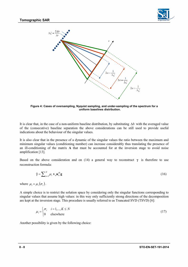
Figure 4 shows the different cases related to 1<≥A . The case 1>A corresponds to a scene extension that is

larger the limit corresponding to the spectral sampling thus generating spatial aliasing of the reconstruction along the elevation. The spectrum is said to be under-sampled and the singular values (generally ordered according to the magnitude) do not show a clear decay thus translating the peculiarity of the acquisition system to induce a loss of information. The case 1=A , previously described corresponds to a sampling at the Nyquist limit: in this case the singular values are all constant in such a way to provide, accordingly to (13) and (14) , the equivalence between A-1 and AH. Finally, the case 1<A corresponds to a scene extension that is smaller than the limit corresponding to the spectral sampling. The spectrum is in this case oversampled, and the oversampling generates a decay of the singular values that translates the redundancy of the sampled information. Such a redundancy can be used to achieve super-resolution in the reconstruction, i.e. Nas 2<δ . A more exhaustive discussion about this topic can be found in [6] [14][15].

STO-EN-SET-191-2014 8 - 7

Tomographic SAR

Figure 4 : Cases of oversampling, Nyquist sampling, and under-sampling of the spectrum for a uniform baselines distribution.

It is clear that, in the case of a non-uniform baseline distribution, by substituting b∆ with the averaged value of the (consecutive) baseline separation the above considerations can be still used to provide useful indications about the behaviour of the singular values.

It is also clear that in the presence of a dynamic of the singular values the ratio between the maximum and minimum singular values (conditioning number) can increase considerably thus translating the presence of an ill-conditioning of the matrix A that must be accounted for at the inversion stage to avoid noise amplification [13].

Based on the above consideration and on (14) a general way to reconstruct γ is therefore to use reconstruction formula:

∑ ==

N

nHnni1

ˆ guvγ µ (16)

where ( )iii σµµ = .

A simple choice is to restrict the solution space by considering only the singular functions corresponding to singular values that assume high values: in this way only sufficiently strong directions of the decomposition are kept at the inversion stage. This procedure is usually referred to as Truncated SVD (TSVD) [6]:

≤=

=elsewhere0

,...,1 NKiii

σµ (17)

Another possibility is given by the following choice:

8 - 8 STO-EN-SET-191-2014

Tomographic SAR

22 ασσµ+

=i

ii (18)

which regularizes the inversion by imposing controlling the square norm of the solution, i.e.:

[ ]2

22minargˆ γLγgγ

γα+−= (19)

where 2⋅ is the L2 norm in C M . The solution provided by the choice in (18) is equivalent to the Wiener filter

[16], in particular to the filter that achieves the solution with a minimum mean square error criterion in the presence of additive white noise.

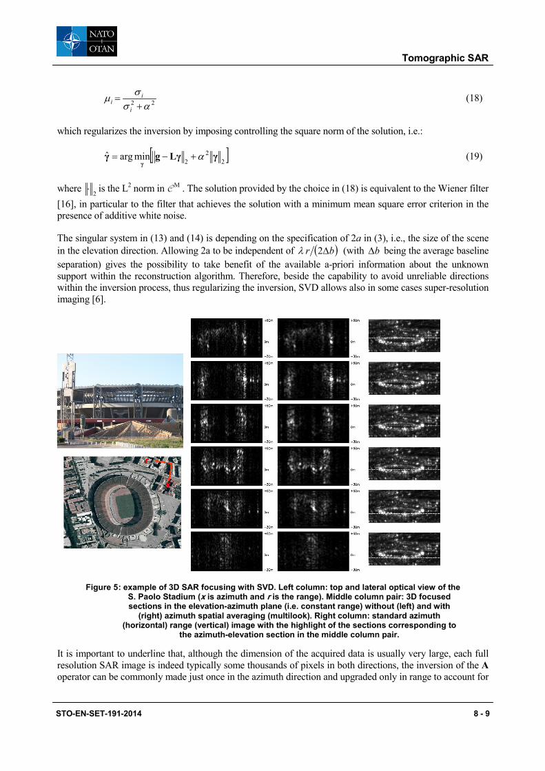
The singular system in (13) and (14) is depending on the specification of 2a in (3), i.e., the size of the scene in the elevation direction. Allowing 2a to be independent of ( )br ∆2λ (with b∆ being the average baseline separation) gives the possibility to take benefit of the available a-priori information about the unknown support within the reconstruction algorithm. Therefore, beside the capability to avoid unreliable directions within the inversion process, thus regularizing the inversion, SVD allows also in some cases super-resolution imaging [6].

Figure 5 : example of 3D SAR focusing with SVD. Left column: top and lateral optical view of the S. Paolo Stadium (x is azimuth and r is the range). Middle column pair: 3D focused sections in the elevation-azimuth plane (i.e. constant range) without (left) and with

(right) azimuth spatial averaging (multilook). Right column: standard azimuth (horizontal) range (vertical) image with the highlight of the sections corresponding to

the azimuth-elevation section in the middle column pair.

It is important to underline that, although the dimension of the acquired data is usually very large, each full resolution SAR image is indeed typically some thousands of pixels in both directions, the inversion of the A operator can be commonly made just once in the azimuth direction and upgraded only in range to account for

STO-EN-SET-191-2014 8 - 9

Tomographic SAR

the variations of the orthogonal baseline components due to the change of the looking geometry. In addition to this, the number of acquisitions is commonly not large; hence the computational cost of the reconstructing algorithm is rather low.

3.2 Capon inversion A more general expression for the evaluation of nγ̂ is given by

gfmHˆ =mγ (20)

where Hmf is the filter for the estimation of ( )mm sγγ = .

Letting [ ]Hg E gg=C , that is the data covariance matrix, a solution obtained from the spectral estimation

theory such that:

1tosubject

minargminargˆ H2

=

=

=

m

ff

af

ffgff

Hm

mgmH

mnmn

E C (21)

i.e., a solution that achieves the minimum output power, subject to unitary gain at the frequency of interest (Capon filter), is provided by [5]:

mm

m

aaa

f 1-g

H

-1g

CC

=m (22)

i.e.:

( )mm aa 1-

gH

2 1ˆC

=msE γ (23)

It is interesting to note that when IC =g , i.e. in the case of a constant data spectrum power, the Capon filtering leads to Nm maf = , i.e. to the classical beam-forming (matched filter). The advantage of the Capon filer is the achievement of high super-resolution for line spectra (i.e. concentrated scatterers along s). However a disadvantage of the Capon filter is the need to estimate the data covariance matrix. This estimation is carried out via spatial averaging (i.e. multilook) thus leading to a loss of spatial resolution.

3.2 Compressed sensing Compressed sensing (CS) [17][18] is a recent technique used in linear inversion problems for signal recovery that takes benefit of the hypothesis that the signal to be reconstructed have (in some basis) a sparse representation, i.e. a small number of non-zero entries. Under certain assumptions of the measurement matrix, the signal can be reconstructed from a small number of measurements.

SAR Tomography in urban areas is a favorable application scenario for CS due to the fact that for typical operative frequencies, the scattering occurs only on some scattering centers associated with ground, façades and roofs of ground structures [19]. From a mathematical point of view CS looks for the best (in the square norm sense) solution of:

8 - 10 STO-EN-SET-191-2014

Tomographic SAR

Aγg = (24)

under the hypothesis that only S<<M entries of γ are different by zero (S=0γ , where

0⋅ is the L0 norm in C M ), with a number of measurements N generally much lower than M . This latter condition is due to the fact that a fine sampling of the output is required to correctly achieve super-resolution reconstructions. In other words CS looks for the solution of the following problem:

ε<−= 20 subject tominargˆ Aγgγγγ

(25)

The problem can be also generalized to the case in which 0γ is close to M but can be assumed sparse under

a linear transformation Bxγ = with MS <=0x where B is not necessary an orthonormal transformation but generally an over-complete dictionary. However, in the case in which SAR Tomography is applied to urban areas the signal is γ has intrinsically a sparse nature ( IB = ).

Under certain conditions it is shown that the solution of the following L1 norm:

ε<−= 21 subject tominargˆ Aγgγγγ

(26)

or equivalently:

{ }21minargˆ Aγgγγ

γ−+= δ (27)

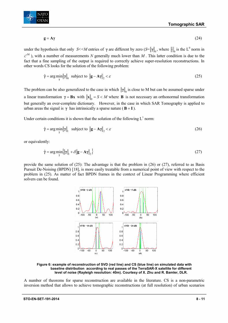
provide the same solution of (25): The advantage is that the problem in (26) or (27), referred to as Basis Pursuit De-Noising (BPDN) [18], is more easily treatable from a numerical point of view with respect to the problem in (25). As matter of fact BPDN frames in the context of Linear Programming where efficient solvers can be found.

Figure 6 : example of reconstruction of SVD (red line) and CS (blue line) on simulated data with baseline distribution according to real passes of the TerraSAR-X satellite for different

level of noise (Rayleigh resolution: 40m). Courtesy of X. Zhu and R. Bamler, DLR.

A number of theorems for sparse reconstruction are available in the literature. CS is a non-parametric inversion method that allows to achieve tomographic reconstructions (at full resolution) of urban scenarios

STO-EN-SET-191-2014 8 - 11

Tomographic SAR

with better performances in terms elevation resolution with respect to BF and SVD [20][21], moreover with respect to Capon inversion it has the advantage of not requiring spatial averaging. The price paid for this improvement is the computational cost that increases: operative tools for processing high resolution data implements joint SVD/CS inversion with CS used in areas where it is expected to have interference of scatterers located at close elevations.

3.0 4D AND MULTID SAR IMAGING

SAR Tomography allows profiling the scattering along the elevation direction. Differential SAR Tomography, also referred to as 4D (3D space + velocity) SAR imaging (focusing) is a natural extension of SAR Tomography for imaging and monitoring targets that exhibit displacements [22][23][24]. It allows measuring the scattering distribution in an elevation–velocity (EV) plane, also known as tomo-doppler plane. For each azimuth and range pixel, the presence of peaks in the EV plane identifies scatterers, possibly interfering in the same resolution cell if more than one peak is present, located at certain elevations and moving with certain velocities.

By referring to Figure 3, where the acquisitions S1 … SN are now supposed to be acquired at different times Ntt ...1 , letting the target P located at elevation s to be characterized by a deformation d(s,tn), we have the

following model for the signal (after de-ramping):

( )

∫−−

≈ dsesg nn tsdjsj

n

,42)( λ

ππζγ (28)

that extends (3) to the presence of movements. The exponential signal related to the deformation can be expanded in Fourier harmonics [23] thus leading to:

( )∫∫ −−= dvdsevsg vjsjDn

nn πηπζγ 224 ,

rbn

n λζ 2

= λ

η nn

t2= (29)

where ν is the Fourier variable associated with nη ; ν measures in ms-1 and assumes the meaning of a velocity (spectral velocity). For linear deformation the spectral velocity coincides with the deformation rate, whereas for more complex motion, ν identifies the (velocity) harmonic involved in the motion.

Inversion of (13) leads to the estimation of the scattering distribution in the EV plane. To this aim, each one of the approaches described for the 3D case in Section 3 can be applied by extending the definition of steering vector as:

[ ] Mmee mNmNmm vjsjvjsjm ,...1,....., 2222T 11 == −−−− πηπζπηπζa , (30)

where M is the product between the number of bins in elevation and velocities of the grid used for the discretization of the 2D integral in (29).

Beside separation of elevations and velocities, 4D SAR imaging allows also the separation of time series of scatterers affected by layover. Furthermore it can be extended to MultiD SAR imaging to account for the presence of specific deformation models (f.i., seasonal and thermal dilations)

8 - 12 STO-EN-SET-191-2014

Tomographic SAR

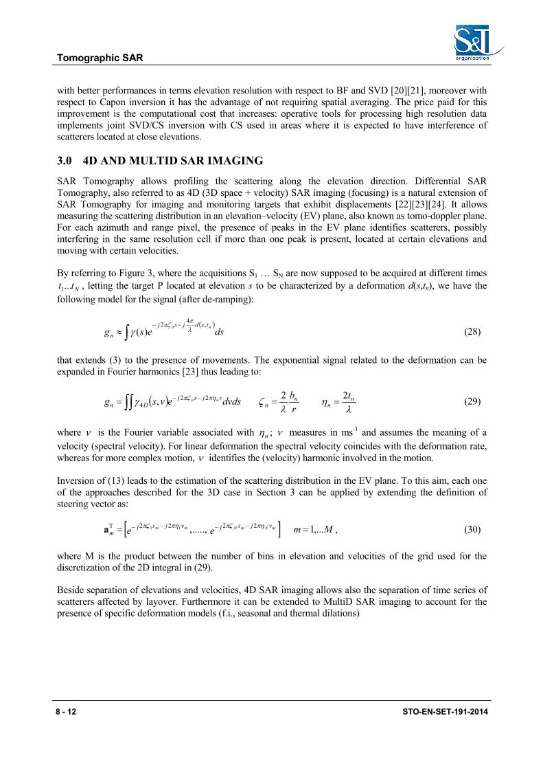
Figure 7 : Example of 4D imaging with medium resolution data of the ENVISAT satellite: The images show the detected single (left) and double (right) scatterers overlaid to a Google

map image. The colour is associated with the mean deformation velocity.

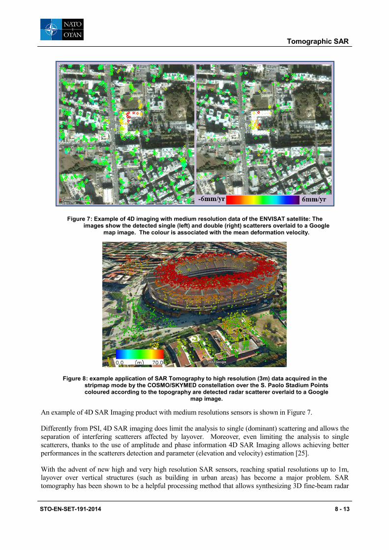
Figure 8 : example application of SAR Tomography to high resolution (3m) data acquired in the stripmap mode by the COSMO/SKYMED constellation over the S. Paolo Stadium Points coloured according to the topography are detected radar scatterer overlaid to a Google

map image.

An example of 4D SAR Imaging product with medium resolutions sensors is shown in Figure 7.

Differently from PSI, 4D SAR imaging does limit the analysis to single (dominant) scattering and allows the separation of interfering scatterers affected by layover. Moreover, even limiting the analysis to single scatterers, thanks to the use of amplitude and phase information 4D SAR Imaging allows achieving better performances in the scatterers detection and parameter (elevation and velocity) estimation [25].

With the advent of new high and very high resolution SAR sensors, reaching spatial resolutions up to 1m, layover over vertical structures (such as building in urban areas) has become a major problem. SAR tomography has been shown to be a helpful processing method that allows synthesizing 3D fine-beam radar

STO-EN-SET-191-2014 8 - 13

Tomographic SAR

scanners from the space capable of solving the layover [25][27] and of achieving improved imaging and monitoring complex structures. Figure 8 shows an example of application of SAR tomography to high resolution data acquired by the COSMO/SKYMED constellation.

4.0 ACKNOWLEDGMENTS

The author wish to acknowledge the European Space Agency (ESA), the Italian Space Agency (ASI) and the National Department of Civil Protection (DPC) for providing the data used for the generation of the images included in this paper. Many thanks also to X. X. Zhu and R. Bamler of DLR for providing the simulated results for Compressive Sensing.

5.0 REFERENCES

[1] A. Moreira, P. Prats-Iraola, M. Younis, G. Krieger, I. Hajnsek, K.P. Papathanassiou, “A tutorial on synthetic aperture radar”, IEEE Geosci. Remote Sens. Magaz., 1 (1), pp. 6-43, 2013.

[2] G. Fornaro, G. Franceschetti, ”SAR Interferometry”, Chapter IV in G.Franceschetti, R.Lanari Synthetic Aperture Radar Processing, CRC-PRESS, Boca Raton, Marzo 1999.

[3] G. Fornaro, V. Pascazio, SAR Interferometry and Tomography: Theory and Applications, Academic Press Library in Signal Processing vol. 2, Elsevier Ltd. 2013

[4] A. Reigber, A. Moreira, “First Demonstration of Airborne SAR Tomography using Multibaseline L-band Data”, IEEE Trans. Geosci. Remote Sens., 38(5), pp. 2142-2152, 2000.

[5] F. Lombardini, M. Montanari, F. Gini, “Reflectivity estimation for multibaseline interferometric radar imaging of layover extended sources”, IEEE Trans. Signal Process., 51, pp. 1508-1519, 2003.

[6] G. Fornaro, F. Serafino, F. Soldovieri, “Three-dimensional focusing with multipass SAR data” IEEE Trans. Geosci. Remote Sens., vol.43 (3), pp.507-517, 2003.

[7] G. Fornaro, F. Lombardini, F. Serafino, “Three-dimensional multipass SAR focusing: experiments with long-term spaceborne data”, IEEE Trans. Geosci. Remote Sens., 43(4), pp. 702-714, 2005.

[8] S. Tebaldini, “Single and Multipolarimetric SAR Tomography of Forested Areas: A Parametric Approach”, IEEE Trans. Geosci. Remote Sens., 48(5), pp. 2375-2387, 2010.

[9] A. Ferretti, C. Prati, F. Rocca, “Nonlinear Subsidence Rate Estimation using Permanent Scatterers in Differential SAR Interferometry”, IEEE Trans. Geosci. Remote Sens., 38, pp. 2202-2212, 2000.

[10] A. Ferretti, C. Prati, F. Rocca, “Permanent Scatterers in SAR interferometry”, IEEE Trans. Geosci. Remote Sens., 39(1), pp. 8-20, 2001.

[11] R.J. Marks, “Introduction to Shannon Sampling and Interpolation Theory”, Spinger-Verlag, 1991, ISBN-10: 146139710

[12] G.H. Golub, C. F. Van Loan, “Matrix Computations”, Johns Hopkins Univ Pr., 1996.

[13] M. Bertero, Linear inverse and ill-posed problems, in Advances in Electronics and Electron Physics, Academic Press, (1989).

8 - 14 STO-EN-SET-191-2014

Tomographic SAR

[14] H.J. Landau, H.O. Pollak, “Prolate Spheroidal Wave Functions, Fourier Analysis and Uncertainties”, The Bell System Tech. J., pp. 65-84, 1960.

[15] D. Slepian, “Prolate spheroidal wave functions, Fourier analysis, and uncertainty – V: The discrete case”, The Bell System Tech. Journal, vol. 57, pp. 1371-1430, May-June 1978.

[16] X. X. Zhu, R. Bamler, “Very High Resolution Spaceborne SAR Tomography in Urban Environment” IEEE Trans. Geosci. Remote Sens, 48 (12), pp. 4296-4308, 2010.

[17] E. J. Candes, M. B. Wakin, “An Introduction To Compressive Sampling”, IEEE Signal Processing Magazine, 25(2), pp. 21-30, 2008.

[18] D.L. Donoho, “Compressed sensing”, IEEE Trans. Inf. Theory, 52(4), pp.1289-1306, 2006.

[19] A. Budillon, A. Evangelista, G. Schirinzi, “SAR Tomography from Sparse Samples, Proc. IEEE Int Geoscience and Remote Sensing Symp. (IGARSS 2009), IV, pp. 865-868, 2009.

[20] A. Budillon, A. Evangelista, G. Schirinzi, “Three-Dimensional SAR Focusing from Multipass Signals Using Compressive Sampling”, IEEE Trans. Geosci. Remote Sens., 49(1), pp. 488-499, 2011.

[21] X. X. Zhu, R. Bamler, “Super-Resolution Power and Robustness of Compressive Sensing for Spectral Estimation With Application to Spaceborne Tomographic SAR”, IEEE Trans. Geosci. Remote Sens, 50(1), pp. 247-258, 2012.

[22] F. Lombardini, “Differential Tomography: a New Framework for SAR Interferometry”, IEEE Trans. Geosci. Remote Sens., 43(1), pp. 37-44, 2005.

[23] G. Fornaro, D. Reale, F. Serafino, “Four-Dimensional SAR Imaging for Height Estimation and Monitoring of Single and Double Scatterers”, IEEE Trans. Geosci. Remote Sens., 47(1), pp. 224-237, 2009.

[24] G. Fornaro, F. Serafino, D. Reale, “4-D SAR Imaging: The Case Study of Rome”, IEEE Geosci. Remote Sens. Lett., 7, pp. 236-240, 2010.

[25] De Maio A., G. Fornaro, and A. Pauciullo (2009), Detection of Single Scatterers in Multdimensional SAR Imaging, IEEE Trans. Geosci. Remote Sens., 47(7), 2284-2997.

[26] D. Reale, G. Fornaro, A. Pauciullo, X. Zhu, R. Bamler, “Tomographic Imaging and Monitoring of Buildings With Very High Resolution SAR Data”, IEEE Geosci. Remote Sens. Lett, 8(4), pp. 661-665, 2011.

[27] X. X. Zhu, R. Bamler , “Demonstration of Super-Resolution for Tomographic SAR Imaging in Urban Environment”, , IEEE Trans. Geosci. Remote Sens., 50 (8), pp.3150-3157, 2012.

[28] G. Fornaro, A. Pauciullo, D. Reale, X. Zhu, R. Bamler, “SAR Tomography: an Advanced Tool for 4D Spaceborne Radar Scanning with Application to Imaging and Monitoring of Cities and Single Building”, IEEE Geosci. and Remote Sens. Soc. Newsletter, pp. 10-20, December 2012.

STO-EN-SET-191-2014 8 - 15

Tomographic SAR

8 - 16 STO-EN-SET-191-2014