University of Nebraska - Lincoln DigitalCommons@University of Nebraska - Lincoln Computer Science and Engineering: eses, Dissertations, and Student Research Computer Science and Engineering, Department of 5-2014 Using a UAV to Effectively Prolong Wireless Sensor Network Lifetime with Wireless Power Transfer Jinfu Leng University of Nebraska-Lincoln, [email protected]Follow this and additional works at: hp://digitalcommons.unl.edu/computerscidiss Part of the Computer Engineering Commons is Article is brought to you for free and open access by the Computer Science and Engineering, Department of at DigitalCommons@University of Nebraska - Lincoln. It has been accepted for inclusion in Computer Science and Engineering: eses, Dissertations, and Student Research by an authorized administrator of DigitalCommons@University of Nebraska - Lincoln. Leng, Jinfu, "Using a UAV to Effectively Prolong Wireless Sensor Network Lifetime with Wireless Power Transfer" (2014). Computer Science and Engineering: eses, Dissertations, and Student Research. 72. hp://digitalcommons.unl.edu/computerscidiss/72
Transcript
University of Nebraska - LincolnDigitalCommons@University of Nebraska - LincolnComputer Science and Engineering: Theses,Dissertations, and Student Research Computer Science and Engineering, Department of
5-2014
Using a UAV to Effectively Prolong Wireless SensorNetwork Lifetime with Wireless Power TransferJinfu LengUniversity of Nebraska-Lincoln, [email protected]
Follow this and additional works at: http://digitalcommons.unl.edu/computerscidiss
Part of the Computer Engineering Commons
This Article is brought to you for free and open access by the Computer Science and Engineering, Department of at DigitalCommons@University ofNebraska - Lincoln. It has been accepted for inclusion in Computer Science and Engineering: Theses, Dissertations, and Student Research by anauthorized administrator of DigitalCommons@University of Nebraska - Lincoln.
Leng, Jinfu, "Using a UAV to Effectively Prolong Wireless Sensor Network Lifetime with Wireless Power Transfer" (2014). ComputerScience and Engineering: Theses, Dissertations, and Student Research. 72.http://digitalcommons.unl.edu/computerscidiss/72
A wireless sensor network is a collection of sensor nodes organized into a coopera-
tive network [13]. Now wireless sensor networks are widely used in many fields,
from habit monitoring to healthcare [2], [6], [32] and [3]. Batteries are currently
the main energy source for the wireless sensor networks. Roundy et al. indicated
that effective energy supplies become the challenge of the applications of wireless
sensor networks, although a few very low power wireless sensor platforms have
entered the marketplace [26]. Current wireless sensor networks deployed for long
periods either require additional infrastructure, such as solar panels, or periodic
maintenance.
In our lab, Griffin and Detweiler proposed a novel solution, using a micro
unmanned aerial vehicle (UAV) to wirelessly charge the sensor nodes and then
prolong the lifetime of the wireless sensor network [11]. UAV has been adopted in
the military world over the last decade and achieved great success [8]. Now there
are a wide range of non-military UAV applications, from autonomous aerial water
sampling [24] to UAV-based remote sensing [22]. Tesla developed the original
idea of wireless power transfer over a century ago [33]. Then recently, researchers
2
have shown that they can significantly and effectively transfer power over medium
distance. For instance, Kurs et al. were able to transfer several tens of watts to fully
light up a 60 W light bulb from distances more than 2 m away [17].
UAV based wireless power transfer system is a very promising solution for
prolonging the sensor network lifetime. First, the sensor nodes are usually dis-
tributed over a large area, and the UAV is able to cover a large area because of
its fast moving speed. At the same time, the UAV is even able to charge sensor
nodes at locations which are normally inaccessible to humans. Second, the wireless
power transfer method makes the charging process easy since no complicated
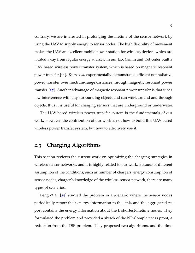
mechanical mechanism is required to operate the sensor node. Fig 1.1 shows a
motivating example of using a UAV to charge sensor nodes. Recently we have
experienced several bridge collapses, such as Minneapolis I35 bridge in 2007 [12].
These disasters would be avoided by deploying wireless sensor nodes on the
bridge to monitor the health of the bridge. The UAV-based wireless power transfer
system is able to maintain the wireless sensor network as a long-term monitoring
system by regularly charge these sensor nodes. In addition, these sensor nodes
even can be embedded into the bridge as some wireless power transfer methods
can work through many materials [28].
If there are many sensor nodes and they are distributed widely, it is a challenge
to decide which nodes should be charged and how much energy should be
transfered. In this thesis, we answer the question: Given the UAV and the sensor
network, what is the most optimal strategy for the UAV so it can prolong the
lifetime of the sensor network as much as possible with a single flight?
There are many possible strategies. For example, one simple strategy is to
let the UAV always fly to next random sensor node and then transfer a random
amount of energy to this sensor node until the UAV has to fly back to the base
3
Figure 1.1: A motivating example of using a UAV to charge sensor nodes
station because of insufficient energy. However, there are a few obvious problems
with this simple strategy. First, the UAV may need to fly back and forth to visit
all these sensor nodes and waste its energy on extra flight. Second, the UAV
may transfer not enough energy to sensor nodes with low energy level but too
much energy to sensor nodes with high energy level, while the sensor network
lifetime is determined by the sensor node with the least energy level. As a result,
the sensor network lifetime is not the optimal, or not even close to the optimal.
There are some other intuitive strategies, including fully charging each sensor
node, transferring a fixed amount of energy to each sensor node, and flying in
the shortest cycle. Also, the UAV is able to use more advanced algorithms if it
has more information about the sensor network, such as the average energy level
4
of all sensor nodes or the exact energy level of each sensor node. However, there
is energy overhead on collecting and maintaining this type of information since
sensor nodes are widely located.
1.1 Contributions
In this thesis, we address the challenge of how to use a UAV to effectively charge
a sensor network. This work partially contributes to a submitted paper [20].
Specially, we
• Give a formal definition of the problem and prove its NP-Completeness. To
the best of our knowledge, this is the first complete NP-Completeness proof
for this problem.
• Propose a series of heuristic algorithms and develop a simulation system to
test them. Since the UAV-based wireless power transfer system is a novel
platform, there is not too much existing research providing related algorithms.
The sensor network energy information can help the UAV to make decisions,
but the sensor network consumes extra resource to provide this information.
Based on this fact, three types of algorithms are discussed.
• Identify the bottleneck of the current system and then guide future devel-
opment. There are many trade-offs while building the UAV-based wireless
power transfer system. It is not straightforward to always make the correct
decision, and it is expensive to build and test different designs. The simula-
tion system can offer insights about these trade-offs and reduce the cost of
the experiments.
5
The rest of this paper is organized as follows. In Chapter 2, we review the
related work, including different approaches to prolong the sensor network lifetime,
main methods of wireless power transfer, and several existing charging algorithms.
In Chapter 3, we then introduce the background, the design of our UAV-based
wireless power transfer system. Next, Chapter 4 gives a formal definition of the
problem and its NP-Completeness proof. Chapter 5 proposes three categories of
algorithms based on their knowledge level of the sensor node energy. In Chapter 6,
we describe a simulation system which is used to evaluate the performance of
different algorithms later. Chapter 7 shows the simulation results and discusses
their implications. We conclude in Chapter 8.
6
Chapter 2
Related Work
The UAV-based wireless power transfer system is a novel platform for prolonging
sensor network lifetime. Many other methods have been proposed to increase the
sensor network lifetime. In section 2.1, we review the existing methods to prolong
the lifetime of sensor networks and discuss their advantages and limitations. Next,
Section 2.2 discusses recent research in wireless power transfer and its combination
with aerial vehicles. Lastly, many researchers focus their efforts on creating
algorithms to allow robots to efficiently traverse the network and charge the nodes.
Section 2.3 introduces current work on optimizing algorithms to improve the
overall charging efficiency.
2.1 Prolonging Wireless Sensor Network Lifetime
Wireless sensor networks consist of sensor nodes mainly powered by small batteries.
After deployment, the small sensor nodes are usually inaccessible to the users,
and thus replacement of the energy source is not feasible [21]. As a result, a
critical limitation of wireless sensor networks applications is the sensor network
7
lifetime. This section briefly reviews the main methods used to prolong the
lifetime of the wireless sensor network. These methods can be divided into three
types, improving energy capacity, reducing energy consumption, and harvesting
environmental energy.
Electrochemical energy, stored in the battery, is the predominant means of
providing power to wireless devices today [26]. Both academia and industry have
been working on improving the energy density of the batteries for decades. For
example, Sim et al. fabricated a micro power source using a micro direct methanol
fuel cell [30]. However, the size of batteries has only decreased mildly while the
size of electronic circuits has decreased by orders of magnitude. Although the
energy density of hydrocarbon fuels used in micro heat engines is very high, they
are not applicable to the wireless sensor nodes because the output power of these
devices is too high and they are not easily to be turned off once started [18].
Sensing and communications consume significant amount of energy in wireless
sensor network. Many researchers have been working on optimizing the data
collecting and data transmission to reduce the energy consumption. Chang and
Tassiulas proposed to adjust the transmitter power level to use the minimum
energy required to reach the intended next hop receiver [7]. Cardei et al. considered
adjusting the sensing range of each sensor node to maximize the sensor network
lifetime for the scenario where a large number of sensors are randomly deployed
to monitor a number of targets [5]. Wang et al. investigated the benefits of adding
a few resource rich mobile nodes to a large number of simple static nodes, where
these resource rich mobile nodes can either act as mobile relays or mobile sinks [34].
Ye et al. developed an energy-efficient medium-access control (MAC) protocol for
wireless sensor networks [36].
There are some other potential energy sources for wireless sensor network.
8
On a bright day, the incident light on the earth surface has a power density of
roughly 100 mW/cm2, and Zhao et al. showed that single crystal silicon solar cells
can achieve efficiency as much as 24.4% [27, 39]. However, in areas or in times
when there is little or no light, the energy density of solar is inadequate. Stordeur
and Stark built a low power thermoelectric generator, which converts thermal
energy directly in electrical energy, so the micro systems have self-sufficient energy
supply [31]. The problem is that it is difficult to get greater than a 10◦C thermal
gradient in a volume of 1 cm3 [27].
Improving battery capacity and optimizing sensing and communications can
slow down the energy consumption of the wireless sensor network, but the
sensor network lifetime is still limited. For harvesting environmental energy, its
continuous work is subject to the environment.
2.2 Wireless Power Transfer
In this section, we briefly introduce the research on the intersections between aerial
vehicles and wireless power transfer.
The vast majority of the previous research focused on supplying power to the
aerial vehicles from ground to improve their flight time. In 1964, a microwave-
powered helicopter was demonstrated to fly 60 f t above a transmitting antenna [4].
In 2011, Achtelik et al. designed a quadcopter platform which broke the micro aerial
vehicle endurance record with laser power beaming [1]. Their work is based on a
powerful infrared laser system. They used complex optics to direct the laser beam
to a special optimized solar cell array equipped on the quadcopter. In this solar
cell array, the laser beam is transformed back to electric energy. In fact, according
to Achtelik et al., this 1 kg quadcopter can achieve unlimited flight time. On the
9
contrary, we are interested in prolonging the lifetime of the sensor network by
using the UAV to supply energy to sensor nodes. The high flexibility of movement
makes the UAV an excellent mobile power station for wireless devices which are
located away from regular energy sources. In our lab, Griffin and Detweiler built a
UAV based wireless power transfer system, which is based on magnetic resonant
power transfer [11]. Kurs et al. experimentally demonstrated efficient nonradiative
power transfer over medium-range distances through magnetic resonant power
transfer [17]. Another advantage of magnetic resonant power transfer is that it has
low interference with any surrounding objects and can work around and through
objects, thus it is useful for charging sensors that are underground or underwater.
The UAV-based wireless power transfer system is the fundamentals of our
work. However, the contribution of our work is not how to build this UAV-based
wireless power transfer system, but how to effectively use it.
2.3 Charging Algorithms
This section reviews the current work on optimizing the charging strategies in
wireless sensor networks, and it is highly related to our work. Because of different
assumption of the conditions, such as number of chargers, energy consumption of
sensor nodes, charger’s knowledge of the wireless sensor network, there are many
types of scenarios.
Peng et al. [25] studied the problem in a scenario where the sensor nodes
periodically report their energy information to the sink, and the aggregated re-
port contains the energy information about the k shortest-lifetime nodes. They
formulated the problem and provided a sketch of the NP-Completeness proof, a
reduction from the TSP problem. They proposed two algorithms, and the time
10
complexity of both are superpolynomial. The core idea of the two algorithms
is to test each permutation of the charging sequence. The difference is that the
preliminary one select the target energy from the current sensor node energy levels
and the more advanced one used a binary search to look for the target energy. They
built a proof-of-concept prototype of the system, and used simulation to study the
proposed algorithms. We believe that their proof is not accurate because the TSP
problem requires that each node to be visited exactly once while the transformed
problem requires that each node to be visited at least once. We provide a more
precise proof based on our definition of problem in Chapter 4. In addition, because
the time complexity of their algorithms are superpolynomial, they are not feasible
for the case where there are a large number of sensor nodes. Also, they studied
the case where the k shortest-lifetime nodes are known, but they did not consider
other cases, such as no energy information at all.
Yoon et al. [37] examined a scenario where the sensor nodes are moving and
that the charging events rely on a fortuitous encounter. Within this scenario, it is
very hard to keep all the sensor nodes alive all the time. The authors used the time
ratio of a node being alive to evaluate the performance of each charging algorithms.
The alive time is assumed to be proportional to the energy consumed by the
node. In addition, they assumed there is a mobile charger with very large energy
capacity. They proposed three basic algorithms: Passive Energy Charging, only
charge nodes with dead battery; Active Energy Charging, charge any encountered
nodes; Restricted Energy Charging, only charge nodes with energy level under a
certain threshold. Through simulation, they found that the performance rank of
algorithms were highly related to the encounter rate. As a result, they proposed the
fourth algorithm, Trend-based Energy Charging, an algorithm like Restricted Energy
Charging but adjusting the value of the threshold according to current encounter
11
rate.
Shi et al. [29] discussed a scenario where a mobile charging vehicle periodically
visits sensor nodes and charges them with wireless power transfer, thus the sensor
network can have unlimited lifetime. They assumed that the charger knows the
energy level of all the sensor nodes and has enough energy to visit and charge all
sensor nodes in a single trip. They studied the problem, given that guaranteeing
unlimited sensor network lifetime is the prerequisite, how to minimize the cost?
Here they defined the cost as working time of the mobile charging vehicle. They
proposed the concept of Renewable Energy Cycle, where the energy level of each
sensor node exhibits periodicity within cycles. A full cycle includes working period
and resting period, based on the status of the mobile charging vehicle, and their
goal is to minimize the percent of working period. First, they offered the necessary
and sufficient conditions for the existence of Renewable Energy Cycle. Second,
they proved that the shortest Hamiltonian cycle is the optimal traveling path by
contradiction. Third, they developed a provable near-optimal algorithm. This work
considers the problem of how to minimize the cost if the mobile charging vehicle
can work multiple times, while we consider the problem of how to maximize
the sensor network lifetime if the mobile charging vehicle only has one working
opportunity.
Zhang et al. [38] defined an interesting scenario, collaborative mobile charging,
where multiple mobile charging vehicles are used to charge sensor nodes and
these charging vehicles are allowed to charge each other. They considered to
maximize the ratio of payload energy (the energy eventually obtained by sensors)
to the overhead energy (energy consumed by chargers’ movements). They had
two significant assumptions. First, the energy transfer efficiencies (base station
to charger, charger to charger, and charger to sensor node) are 1.0. Second,
12
the charging time is negligible compared to the traveling time. Moreover, they
restricted their work on 1-D wireless sensor networks to reduce the complexity.
For homogeneous case where all sensors consume energy at the same rate, they
indicated that the payload energy is fixed in a charging cycle and the goal is
equivalent to minimizing the overhead energy (i.e., the total moving distance of
chargers). They proposed to let these chargers meet at some rendezvous points
and concentrate their residual energy to a few chargers to reduce the total moving
distance. For heterogeneous case where sensors have various energy consumption
rate, they presented a heuristic algorithm. The main idea of this algorithm is to
cluster the sensor nodes into groups and then employs the previous algorithm (the
algorithm for homogeneous case) to these groups. We consider that their proposed
algorithms are not applicable to our UAV-based wireless power transfer system
because their two assumptions, 1.0 transfer efficiency and negligible charging
time, are not practical for our system, or even any existing wireless power transfer
system.
Johnson et al. [15] already studied using the UAV-based wireless power transfer
system, built by Griffin and Detweiler [11], to prolong the sensor network lifetime.
Their work focused on the scenario where the UAV can have multiple flights but it
can only charge a single node in every single flight. Regarding the wireless sensor
network, they explored five different sink positioning algorithms and found that
Greedy Heuristic and LP sink selection algorithms performed well. Regarding
charging, they found that charging the sensor node with the least energy level is
the best sensor node selection strategy. In our work, we removed the restriction
that the UAV can only charge a single sensor node during a flight.
13
Chapter 3
Background
3.1 System Overview
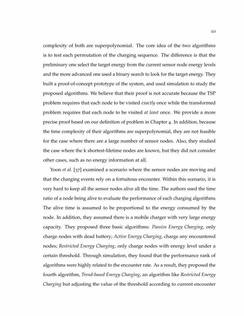
Fig. 3.1 shows an overview of the hardware of the UAV-based wireless power
transfer system. The three main components are the UAV, the wireless power
transfer system and the sensor node localization system.
Our basic UAV platform is an Ascending Technologies Hummingbird quad-
copter. The UAV is light weight and agile. We give more details of the UAV in
section 3.2.
The wireless power transfer system consists of the power transmission part and
power receiver part. The power transmission part is deployed on the UAV and it
consists of a plastic frame, a drive board and coils. The plastic frame holds the
transmitting coils and the drive board on the UAV. The power receiver part consists
of a receiver board, coils, and a sensor node that is specific to the application, such
as vibration, temperature, soil moisture, or pressure sensing. In this paper we omit
any application specific sensing system and instead focus on the wireless power
transfer and the sensor node localization. We give more details of the wireless
14
Figure 3.1: The UAV-based wireless power transfer system (Andrew Mittleider).
power transfer system in section 3.3.
The sensor node localization system can guide the UAV to achieve more
accurate localization than only using GPS data. It consists of a magnetic resonant
sensor and an optical flow camera. The magnetic resonant sensor is supposed
to be deployed with the the power receiver part. The magnetic resonant sensor
can be used to estimate the distance between the UAV and itself by measuring
the voltage. The optical flow camera, mounted on the bottom of the UAV, can
provide accurate relative motion estimates. Combining the estimated distance and
the estimated relative motion, the UAV is able to localize the magnetic resonant
sensor with decent error. More details can be found in section 3.4.
The UAV power transfer system is controlled by a computer station. The
computer station runs Robot Operating System (ROS), which provides a collection
15
ху
z
T1
Front Right Rotor
T4
Back Right Rotor
T2
Front Left Rotor
T3
Back Left Rotor
θψ
ø
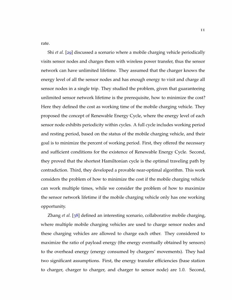
Figure 3.2: The schematic of the UAV (Andrew Mittleider). Rotors 1 and 3 spin inone direction, while rotors 2 and 4 spin in the opposite direction, yielding
opposing torques for control.
of libraries and tools for developing robot applications [10]. We use ROS to control
the overall system and operate the communication. The computer station has two
separate 802.15.4 (Zigbee) radio links operating at 2.4GHz. One of the Zigbee links
is used for the flight of the UAV and the other is dedicated to the power transfer
and localization.
3.2 UAV
Fig. 3.2 shows the schematic of the UAV. It has four rotors. Different spinning
speed of the rotor will produce different thrust and torque about the center of the
rotor. If the thrust and torque from all sides are equal, the vehicle will produce
force only in the z-axis direction. Unequal thrust and torque will cause rotational
moments around ψ, θ, or φ and force moments in the x-axis or y-axis direction.
16
The UAV is 368 g without battery and 543 with the battery. It has a recom-
mended maximum payload of 200 g, and our experiment results show that the
UAV is capable to carry object up to 400 g. We are interested finding an optimal
UAV velocity so that the UAV can minimize the energy cost for reaching the sensor
nodes. Andrew Mittleider did comprehensive experiments and determined that
the optimal speed for the UAV we are using is 7.3 m/s. In fact, results show that
with a single battery by flying at the speed of 7.3 m/s the UAV can fly for 2.7 km
more than flying at 9.5 m/s and 3.5 km more than flying at 3 m/s.
3.3 Wireless Power Transfer
In our lab, Brent Griffin designed and built the wireless power transfer system as
discussed below.
An AD9833 programmable waveform generator is the main component of the
TX Drive Board. In our system, we use the waveform generator to generate a signal
at 165 KH. The frequency of the generated wave can be tuned online to increase
power transfer or utilize different coils. This signal is input into an H-Bridge that
generates a high-power alternating current that is driven through the TX Drive
Coil. A processor is integrated into the TX Drive Board to control the frequency,
enable or disable power transfer, monitor voltage and current, and communicate
with the ground sensors and the computer station. The Drive Board sends an
alternating current through the TX Drive Coil causing an alternating magnetic
field that drives the neighboring TX Resonant Coil. The TX Resonant Coil focuses
the magnetic field to the RX Resonant Coil for transmission. The RX Resonant Coil,
which is placed near the sensor node, receives power from the magnetic field, then
the power is inductively transferred to the RX load coil. The Rx Receiver Board
17
is connected to the RX Load Coil to draw energy from the RX Resonant Coil and
then provide to the sensor node. For additional details see [11].
3.4 Sensor Node Localization
To charge a sensor node, the UAV need to localize this sensor node at first. GPS
data is good to lead the UAV to the rough location of the sensor node, but GPS
data has up to 7.8 m error in a 95% confidence range [9]. As a result, sole GPS data
is insufficient for sensor node localization in our application, since the UAV must
be within 30 cm for efficient wireless power transfer. Andrew Mittleider designed
and built the sensor node localization system to achieve more accurate localization
as discussed below.
A MR Sensor Node, including a MR Sensor Board and a MR Sensor Coil, is
used to assist more accurate localization. The MR Sensor Node measures the
voltage through the a MR Sensor Coil. The voltage measurements are then be
sent to the computer station over a short-range radio. We are able to estimate
the distance between the UAV and the MR Sensor Node through the measured
voltage. At the same time, the equipped optical flow camera can provide accurate
relative motion estimates over short periods of time [16, 35]. The UAV starts by
going to points in a square surrounding the initially estimated position while
simultaneously calculating the position of the sensor node based on the voltage
and relative motion measurements. After the last waypoint is reached, the UAV
flies to the estimated position of the sensor node.
The experiment results show an average error of 27 cm, with a maximum of
48 cm, and an average localization time of 36 seconds. At 27 cm, the wireless power
transfer rate is at 98.6% of the maximum [20].
18
Chapter 4
Problem Definition and
NP-Completeness Proof
We begin by talking about the intuition of the problem. Then we formally describe
the problem and give the decision version of the problem. At the end, we show
that the problem is NP-Complete by reduction from Metric-TSP [19]. Metric-TSP is
a special case of Traveling Salesman Problem (TSP) where the intercity distances
satisfy the triangle inequality thus the direct connection between two cities is never
farther than a route via intermediate cities.
4.1 Problem Intuition
Usually a group of wireless sensor nodes is distributed on a field with a pre-
designed scheme. The number of sensor nodes and the size of the field may vary
depending on the application. We assume that all the sensor nodes have a constant
energy consumption rate for simplicity. For our system, we assume the UAV starts
at a fixed or mobile base station near the sensor network field. The UAV starts with
19
full energy capacity from the base station and returns to the base station for further
maintenance and recharging after it finishes its work. During the working time,
the UAV is either flying from one location to another location, or it is hovering
to charge a sensor node. To reduce the complexity of the proof we assume that
the energy consumption rate of hovering is 0 in the formal problem definition. In
addition, the UAV needs a process to localize the sensor node before charging.
This is because that the GPS data is not accurate enough to lead the UAV to a
satisfied position to achieve good transfer efficiency. For the sake of simplicity, we
do not include the localization process in our formal definition of the problem.
However, we do consider this process in our simulation experiments, as discussed
in Chapter 6 and Chapter 7. We also assume that the UAV transfers power at a
constant rate to the sensor node with a constant transfer efficiency. The goal of our
work is to use a system like this to prolong the sensor network lifetime as much as
possible.
4.2 Problem Definition
We now present a formal definition of this problem, and we call it UAVWS
(UAV Wireless Power Transfer for Sensor Network). Fig. 4.1 shows a visual
representation of the problem. We begin by defining the problem in a graph
G = (V, E), V = {vbase} ∪Vnodes, where vbase is the base station and each vertex of
the Vnodes is a sensor node that may need to be charged. Base station and sensor
nodes are connected through edges of possible UAV flight paths, E. The UAV is
able to travel along edges in E and stop at nodes in Vnodes to charge the sensors. The
UAV also consumes energy at a rate of ec f while flying and ect while transferring
energy. The total energy consumed by the UAV cannot exceed energy capacity,
20
Figure 4.1: A representation of the UAV, UAV base station, and sensor nodesalong with the different variables used in the algorithm.
EUAV of the UAV. These variables and notations are summarized in Table 4.1.
The system is said to be dead when the energy of any of the sensor nodes is 0.
It is constrained such that the initial location of the UAV is at vbase and the UAV
must return to vbase before it consumes all of its energy. When the UAV is at vertex
A, where A ∈ V, it has two types of valid actions. It can move to vertex B, where
B ∈ V and edge (A, B) ∈ E, or it can stay at A and charge A, if A ∈ Vnodes, for
a time of t, where t ∈ R+. The optimization version of the problem is stated as:
What is the longest lifetime the system can achieve? The decision version of the
problem is stated as: Given the values of the variables (G, vbase, Vnodes, EUAV , ec f ,
ect, r, v, Ei, ei), is there a finite sequence of valid UAV actions that can keep the
system alive until time T?
21
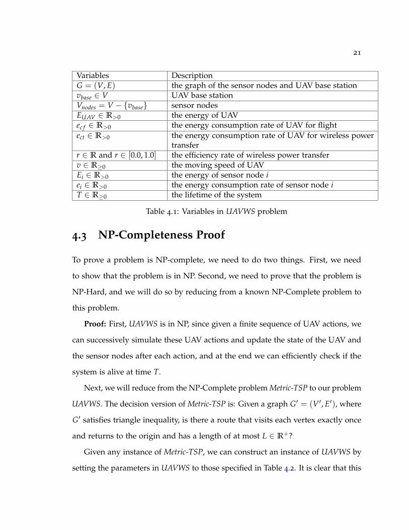
Variables DescriptionG = (V, E) the graph of the sensor nodes and UAV base stationvbase ∈ V UAV base stationVnodes = V − {vbase} sensor nodesEUAV ∈ R>0 the energy of UAVec f ∈ R>0 the energy consumption rate of UAV for flightect ∈ R>0 the energy consumption rate of UAV for wireless power
transferr ∈ R and r ∈ [0.0, 1.0] the efficiency rate of wireless power transferv ∈ R≥0 the moving speed of UAVEi ∈ R>0 the energy of sensor node iei ∈ R>0 the energy consumption rate of sensor node iT ∈ R≥0 the lifetime of the system
Table 4.1: Variables in UAVWS problem
4.3 NP-Completeness Proof
To prove a problem is NP-complete, we need to do two things. First, we need
to show that the problem is in NP. Second, we need to prove that the problem is
NP-Hard, and we will do so by reducing from a known NP-Complete problem to
this problem.
Proof: First, UAVWS is in NP, since given a finite sequence of UAV actions, we
can successively simulate these UAV actions and update the state of the UAV and
the sensor nodes after each action, and at the end we can efficiently check if the
system is alive at time T.
Next, we will reduce from the NP-Complete problem Metric-TSP to our problem
UAVWS. The decision version of Metric-TSP is: Given a graph G′ = (V′, E′), where
G′ satisfies triangle inequality, is there a route that visits each vertex exactly once
and returns to the origin and has a length of at most L ∈ R+?
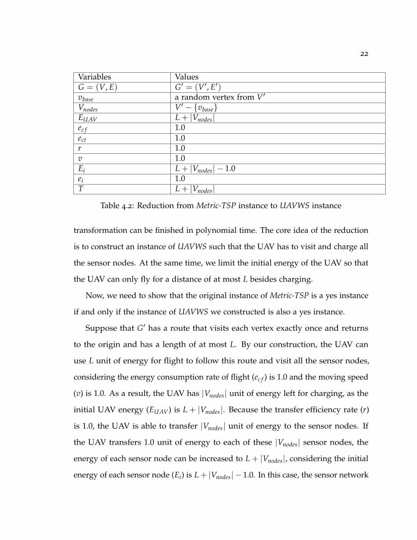
Given any instance of Metric-TSP, we can construct an instance of UAVWS by
setting the parameters in UAVWS to those specified in Table 4.2. It is clear that this
22
Variables ValuesG = (V, E) G′ = (V′, E′)vbase a random vertex from V′
Vnodes V′ − {vbase}EUAV L + |Vnodes|ec f 1.0ect 1.0r 1.0v 1.0Ei L + |Vnodes| − 1.0ei 1.0T L + |Vnodes|
Table 4.2: Reduction from Metric-TSP instance to UAVWS instance
transformation can be finished in polynomial time. The core idea of the reduction
is to construct an instance of UAVWS such that the UAV has to visit and charge all
the sensor nodes. At the same time, we limit the initial energy of the UAV so that
the UAV can only fly for a distance of at most L besides charging.
Now, we need to show that the original instance of Metric-TSP is a yes instance
if and only if the instance of UAVWS we constructed is also a yes instance.
Suppose that G′ has a route that visits each vertex exactly once and returns
to the origin and has a length of at most L. By our construction, the UAV can
use L unit of energy for flight to follow this route and visit all the sensor nodes,
considering the energy consumption rate of flight (ec f ) is 1.0 and the moving speed
(v) is 1.0. As a result, the UAV has |Vnodes| unit of energy left for charging, as the
initial UAV energy (EUAV) is L + |Vnodes|. Because the transfer efficiency rate (r)
is 1.0, the UAV is able to transfer |Vnodes| unit of energy to the sensor nodes. If
the UAV transfers 1.0 unit of energy to each of these |Vnodes| sensor nodes, the
energy of each sensor node can be increased to L + |Vnodes|, considering the initial
energy of each sensor node (Ei) is L+ |Vnodes| − 1.0. In this case, the sensor network
23
lifetime can be prolonged to the desired time (T), L + |Vnodes|, considering the
energy consumption rate of each sensor node (ei) is 1.0. Therefore, our constructed
instance is a yes instance if the instance of Metric-TSP is a yes instance.
Now suppose that our constructed instance of UAVWS is a yes instance, where
the UAV can follow a sequence of UAV actions and then no sensor node is dead
before the desired time (T), L + |Vnodes|. Because each sensor node needs to be
charged at least 1.0 unit of energy to be alive until time T, |Vnodes| unit of energy is
required for charging in total. As a result, the UAV has at most L unit of energy for
flight and thus it can fly a distance of at most L. Therefore, G must have a route
that covers all these |Vnodes| sensor nodes and returns to the origin and the distance
is at most L. Consequently, G′ must have a route that visits each vertex exactly
once and returns to the origin and has a length of at most L. This is because that if
a vertex is previously visited we can simply remove it from the route and directly
connect the previous vertex and the next vertex to guarantee that no vertex will be
visited more than once. At the same time, the triangle inequality of the edges can
warrant that the distance of the updated route will never be farther then the origin
one. Therefore, the instance of Metric-TSP is a yes instance if our constructed
instance is a yes instance.
We have shown that UAVWS is in NP, and proved that the original instance of
Metric-TSP is a yes instance if and only if the constructed instance of UAVWS is a
yes instance. Therefore, UAVWS is NP-Complete.
24
Chapter 5
Algorithms
In this chapter, we develop a set of heuristic algorithms for selecting the nodes to
charge. We evaluate their performance in the Chapter 7.
The UAV is assumed to be able to know the energy level of a node when it is
nearby. When the UAV just starts from the base station, it may have no knowledge,
some knowledge, or complete knowledge of the sensor node energy level. We
separate the algorithms based on knowledge levels because that the UAV is able to
use more advanced algorithms with more available information but in practical
applications there is overhead on maintaining this information.
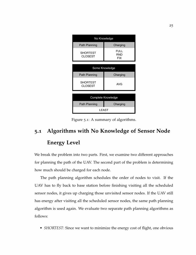
For the three categories, there are nine total algorithms. Fig. 5.1 summarizes all
the nine algorithms. For No Knowledge category, there are six algorithms, combining
two path planning algorithms (SHORTEST and CLOSEST) and three charging
algorithms (FULL, RND and FIX). For Some Knowledge category, there are two
algorithms, combining two path planning algorithms (SHORTEST and CLOSEST)
and one charging algorithm (AVG). There is one specific algorithm for Complete
Knowledge category. The details of these algorithms are discussed in the following
sections.
25
Figure 5.1: A summary of algorithms.
5.1 Algorithms with No Knowledge of Sensor Node
Energy Level
We break the problem into two parts. First, we examine two different approaches
for planning the path of the UAV. The second part of the problem is determining
how much should be charged for each node.
The path planning algorithm schedules the order of nodes to visit. If the
UAV has to fly back to base station before finishing visiting all the scheduled
sensor nodes, it gives up charging those unvisited sensor nodes. If the UAV still
has energy after visiting all the scheduled sensor nodes, the same path planning
algorithm is used again. We evaluate two separate path planning algorithms as
follows:
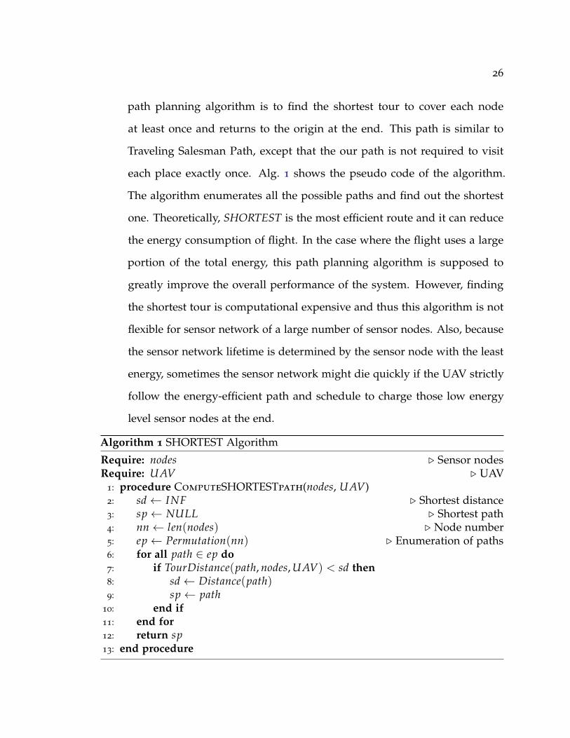
• SHORTEST: Since we want to minimize the energy cost of flight, one obvious
26
path planning algorithm is to find the shortest tour to cover each node
at least once and returns to the origin at the end. This path is similar to
Traveling Salesman Path, except that the our path is not required to visit
each place exactly once. Alg. 1 shows the pseudo code of the algorithm.
The algorithm enumerates all the possible paths and find out the shortest
one. Theoretically, SHORTEST is the most efficient route and it can reduce
the energy consumption of flight. In the case where the flight uses a large
portion of the total energy, this path planning algorithm is supposed to
greatly improve the overall performance of the system. However, finding
the shortest tour is computational expensive and thus this algorithm is not
flexible for sensor network of a large number of sensor nodes. Also, because
the sensor network lifetime is determined by the sensor node with the least
energy, sometimes the sensor network might die quickly if the UAV strictly
follow the energy-efficient path and schedule to charge those low energy
level sensor nodes at the end.
Algorithm 1 SHORTEST Algorithm
Require: nodes . Sensor nodesRequire: UAV . UAV
1: procedure ComputeSHORTESTpath(nodes, UAV)2: sd← INF . Shortest distance3: sp← NULL . Shortest path4: nn← len(nodes) . Node number5: ep← Permutation(nn) . Enumeration of paths6: for all path ∈ ep do7: if TourDistance(path, nodes, UAV) < sd then8: sd← Distance(path)9: sp← path
10: end if11: end for12: return sp13: end procedure
27
• CLOSEST: It is a greedy algorithm to always move to the closest unvisited
sensor node until all the nodes are visited. Alg. 2 shows the pseudo code of
the algorithm. The status of all the nodes are initiated as unvisited. Then the
algorithm uses loops to find the next closest unvisited node, add it to the
path, and set its status to visited, until all the nodes are added to the path.
The time complexity of the algorithm is polynomial, so it is applicable to the
sensor network of a large number of sensor nodes. At the same time, the
implementation of the algorithm is straightforward and easy. The problem is
that the UAV may need to move back and forth several times and then waste
its energy on flight. Also, the sensor nodes with low energy level might be
located far away and then be ignored at the beginning. As a result, these
sensor nodes may use up their energy before the UAV starts charging them.
The charging algorithm determines the amount of energy to transfer from the
UAV to the node. We evaluate three different charging algorithms as follows:
• FULL: It charges each candidate node to its full capacity. FULL can reduce
the ratio of overhead (flight and localization), regarding energy consumption.
However, charging each node to its full capacity means that the UAV may be
unable to visit every node in the network due to its own energy limitations.
• RND: It charges each candidate node with a random amount of energy. The
random value is generated in the range from 0 to the amount of used energy.
RND decreases the possibility of the case where the UAV charges a few sensor
nodes and leave most sensor nodes uncharged. However, this algorithm may
have the problem of charging too much energy to sensor nodes with high
energy level and charging too few energy to sensor nodes with low energy
level. As a result, the energy is not distributed effectively to sensor nodes.
28
Algorithm 2 CLOSEST Algorithm
Require: nodes . Sensor nodesRequire: UAV . UAV
1: procedure ComputeSHORTESTpath(nodes, UAV)2: cl ← UAV[′location′] . Current location3: cp← [] . CLOSEST Path4: nn← len(nodes) . Node number5: for i = 0 to nn− 1 do6: nodes[i][′visited′]← False7: end for8: for i = 1 to nn do9: cd← INF . Closest distance
10: cn← −1 . Closest node11: for j = 0 to nn− 1 do12: if nodes[j][′visited′] == False and Distance(cl, nodes[j][′location′]) <
cd then13: cd← Distance(cl, nodes[j][′location′])14: cn← j15: end if16: end for17: cl ← nodes[cn][′location′]18: nodes[cn][′visited′]← True19: cp.append(cn)20: end for21: return cp22: end procedure
• FIX: It charges each candidate node with a fixed amount of energy. Although
FIX is not optimal as sensor nodes with lower energy level should be charged
with more energy, it guarantees that each sensor node gets a roughly equal
amount of energy. It is supposed to work well for the case where the initial
energy levels of sensor nodes are close, but work poorly for the case where
the initial energy levels of sensor nodes are very different. Also, another
problem is that it is hard to determine the value of the fixed amount. A small
value may increase the ratio of energy consumption overhead, and a large
value may lead to that the UAV does not have enough energy to charge the
29
sensor nodes which are scheduled to visit at the end.
Combining two path planning algorithms and three charging algorithms there
are six total algorithms in this category.
5.2 Algorithms with Some Knowledge of Sensor
Node Energy Level
Because the lifetime of the whole system is determined by the node with the
least energy level, an intuitive idea is to firstly charge nodes whose energy levels
are below the average. Olfati-Saber and Shamma introduced a distributed filter
that allows the nodes to track the average of multiple measurements using an
average consensus based distributed filter [23]. We consider the case where the
UAV knows the initial average energy level of all the sensor nodes, and then uses
this knowledge to guide its behavior. We call this charging algorithm AVG, and the
UAV charges each candidate node to the initial average energy level of the sensor
network. However, the potential problem is that the UAV may fly around and
do nothing when all the sensor nodes are already charged to the initial average
energy level. This is likely to occur when all the sensor nodes have similar initial
energy or the UAV has a very large energy capacity.
We still evaluate two separate path planning algorithms SHORTEST and CLOS-
EST, as described in last section 5.1.
Combining two path planning algorithms and one charging algorithm there
are two total algorithms in this category.
30
5.3 Algorithms with Complete Knowledge of Sensor
Node Energy Level
We have one more algorithm, LEAST, which requires the knowledge of the exact
energy level of each sensor node at the beginning. The LEAST algorithm schedules
its path based on the energy level of sensor nodes. It starts from the sensor node
with the least power, then move to sensor node with second least power, and so
forth. Although this path is not the most energy-efficient, it makes sure that sensor
nodes with low energy level can be charged at the beginning. Because the energy
level of each sensor node and the scheduled path is known, the UAV is able to
compute how much energy is required for flying, localization and hovering, and
then the UAV knows how much energy can be effectively transfered to sensor
nodes. At the end, it computes a value as target energy, and charges all the
candidate nodes to this target energy.
The algorithm used to compute this target energy is demonstrated in Alg. 3.
It uses a loop to enumerate the number of sensor nodes to be charged, computes
their corresponding optimal values of target energy, and finds out the overall best.
Given the number of sensor nodes to be charged, it firstly computes the amount of
energy which can be effectively received by sensor nodes. Next, the corresponding
optimal target energy is computed by a helper function BINARYSEARCHTARGET,
which uses binary search to narrow the range of the optimal target energy until
the result satisfies the accuracy requirement.
The LEAST algorithm in practice performs extremely well (details discussed in
the Chapter 7), even though it is not optimal theoretically. We can improve LEAST
in the path planning part by finding the shortest cycle to cover all the candidate
nodes and thus more energy can be used for charging sensor nodes. The problem
31
Algorithm 3 Compute Target Energy for LEAST Algorithm
Require: nodes . Sensor nodesRequire: UAV . UAV
1: procedure ComputeTargetEnergy(nodes, UAV)2: sn← SortByEnergy(nodes) . Sorted nodes3: te← 0 . Target energy4: nn← len(sn) . Node number5: for i = 1 to nn do6: cn← sn[0 : i] . Candidate nodes, the first i nodes of the sorted nodes7: te← UAV[′energy′] . Total energy8: te← te− FlyingCost(cn, UAV)9: te← te− LocalizationCost(cn, UAV)
10: te← te− HoveringCost(cn, UAV)11: ee← te ∗ trans f erRate . Efficient energy for sensor nodes12: cte← BinarySearchTarget(ee, cn) . Current target energy13: if i < nn then14: cte← min(cte, nodes[i][′energy′])15: end if16: te← max(te, cte)17: end for18: return te19: end procedureRequire: ee . Efficient energyRequire: cn . Candidate nodes20: procedure BinarySearchTarget(ee, cn)21: lb← cn[0][′energy′] . Left bound22: rb← lb + ee . Right bound23: while (rb− lb) > AccurancyRequirement do24: m← (rb + lb)/225: re← 0 . Required energy26: for i = 0 to len(cn)− 1 do27: if cn[i][′energy′] < m then28: re← re + m− cn[i][′energy′]29: end if30: end for31: if re < ee then32: lb← m33: else34: rb← m35: end if36: end while37: return lb38: end procedure
32
is that finding the shortest cycle is computationally expensive and thus it is not
feasible for sensor networks with a large number of sensor nodes. In some extreme
cases, the charging part of LEAST may fail. For example, the second sensor node
may die before the UAV finishes charging the first sensor node. However, in
practice, this is very unlikely to happen. This is because the chance that several
sensor nodes are dying while the UAV is charging another sensor node is very low
considering that the charging only takes a few minutes and the full lifetime of a
sensor node is tens of days. Also, the path planning algorithm of starting from the
sensor nodes with lower energy even further reduces the probability.
We should note that the LEAST algorithm assumes that the UAV has complete
knowledge of sensor node energy level, and there is overhead to maintain this
knowledge in real life. At this point, the information of sensor nodes’ energy
consumption rates is not assumed to be available to the UAV. If this information is
available, LEAST can be improved by computing individual target energy for each
sensor node. For example, if a sensor node has a higher energy consumption rate,
LEAST could be modified to charge it to a higher target energy.
33
Chapter 6
Simulation System
We developed a simulation system to test the performance of the nine algorithms
discussed in Chapter 5 and explore the impacts of a series of system parameters.
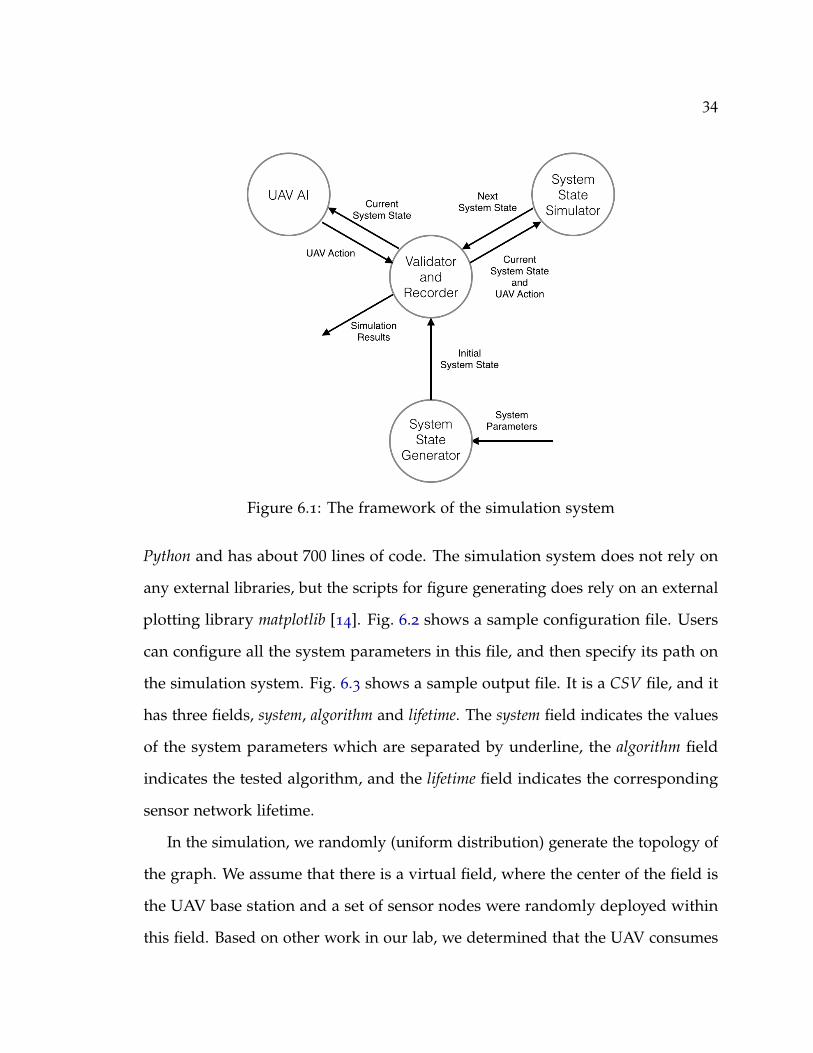
Fig. 6.1 shows the framework of the simulation system. It consists of four main
components, System State Generator, UAV AI, System State Simulator, and Validator
and Recorder. System State Generator takes the system parameters as the input and
then generates the initial system state. UAV AI takes the current system state
as input and returns the UAV action as output. System State Simulator takes the
current system state and UAV action as input and returns the next system state as
output. Validator and Recorder connects the other components, validates the data,
and records the simulation results.
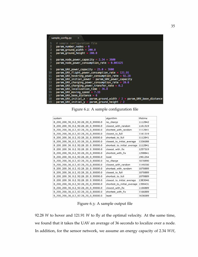
The simulation system gets the values of all system parameters by reading
a configuration file. Every system parameter can have a list of possible values,
and then the simulation system will test all the combinations of these values. The
simulation system writes the simulation results (system parameters, algorithm
name, and sensor network lifetime) to specified output files, which are then used
by other scripts to generate figures. The simulation system is implemented in
34
Figure 6.1: The framework of the simulation system
Python and has about 700 lines of code. The simulation system does not rely on
any external libraries, but the scripts for figure generating does rely on an external
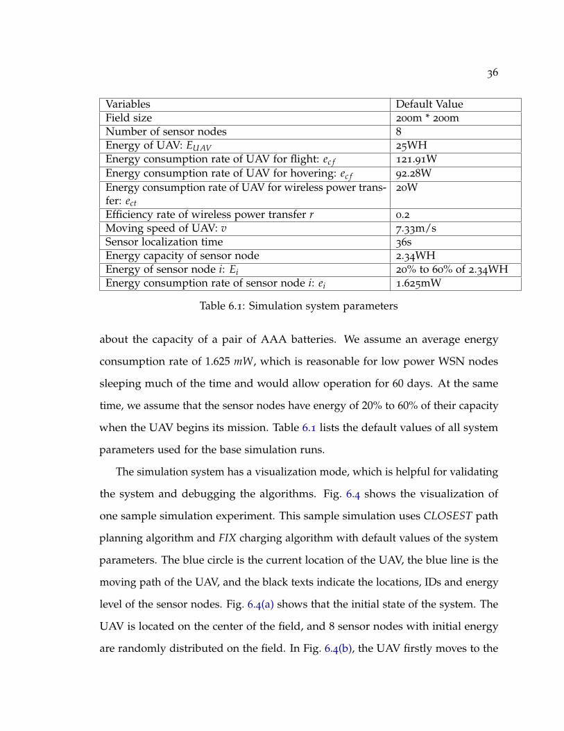
Energy of UAV: EUAV 25WHEnergy consumption rate of UAV for flight: ec f 121.91WEnergy consumption rate of UAV for hovering: ec f 92.28WEnergy consumption rate of UAV for wireless power trans-fer: ect
20W
Efficiency rate of wireless power transfer r 0.2Moving speed of UAV: v 7.33m/sSensor localization time 36sEnergy capacity of sensor node 2.34WHEnergy of sensor node i: Ei 20% to 60% of 2.34WHEnergy consumption rate of sensor node i: ei 1.625mW
Table 6.1: Simulation system parameters
about the capacity of a pair of AAA batteries. We assume an average energy
consumption rate of 1.625 mW, which is reasonable for low power WSN nodes
sleeping much of the time and would allow operation for 60 days. At the same
time, we assume that the sensor nodes have energy of 20% to 60% of their capacity
when the UAV begins its mission. Table 6.1 lists the default values of all system
parameters used for the base simulation runs.
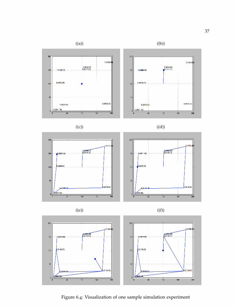
The simulation system has a visualization mode, which is helpful for validating
the system and debugging the algorithms. Fig. 6.4 shows the visualization of
one sample simulation experiment. This sample simulation uses CLOSEST path
planning algorithm and FIX charging algorithm with default values of the system
parameters. The blue circle is the current location of the UAV, the blue line is the
moving path of the UAV, and the black texts indicate the locations, IDs and energy
level of the sensor nodes. Fig. 6.4(a) shows that the initial state of the system. The
UAV is located on the center of the field, and 8 sensor nodes with initial energy
are randomly distributed on the field. In Fig. 6.4(b), the UAV firstly moves to the
37
((a)) ((b))
((c)) ((d))
((e)) ((f))
Figure 6.4: Visualization of one sample simulation experiment
38
sensor node 6 since this is the closest sensor node to the UAV. Fig. 6.4(c) shows
that the UAV successively charges sensor node 6, 1, 7, 3, 5, 0, 2 and 4. At this point,
the UAV has visited all the sensor nodes. In Fig. 6.4(d), the UAV begins a new
round of charging and starts from sensor node 4 and 2. Fig. 6.4(e) shows that in
the second round of charging the UAV has visited sensor node 4, 2, 5, 0, 3 and is
moving to sensor node 6. Fig. 6.4(f) shows the final state of the system. We can
notice that the UAV has to fly back to the base station before complete its charging
at sensor node 6.
In next section, we use the average sensor network lifetime to compare the
performance of the nine algorithms. For each configuration of the system param-
eters, we run all the algorithms 100 times. The running time of the simulation
depends on the values of the system parameters. It takes about 30 minutes for the
simulation system to test all the algorithms 100 times with default values of the
system parameters.
39
Chapter 7
Results
7.1 Introduction
In this chapter, we test the algorithms with different system configurations. On
the one hand, we are interested in comparing and summarizing these algorithms’
performance in different situations. On the other hand, we want to explore the
influence of these system parameters and then guide the development of the
UAV-based wireless power transfer system.
Based on the requirements of real world applications, the field size of sensor
network and the number of sensor nodes may change. In Section 7.2 and Section 7.3,
we evaluate simulation results to determine the performance of the algorithms
with varying size of sensor network field or varying number of sensor nodes.
Also, the UAV base station may not be able to be located in the center of every
sensor network field in consideration of the operation cost. For example, several
sensor networks may need to share a centralized UAV base station. We have an
experiment in Section 7.4 to explore the impact of the distance from the UAV base
station to the sensor network.
40
In addition, at this point, it requires 36 seconds for the UAV to locate a sensor
node before charging. The localization time might be greatly reduced with a better
localization algorithm and thus the overhead of charging a sensor node can be
reduced. Section 7.5 explores the impact of an improved localization time.
The UAV itself has a very limited energy capacity now. For example, the UAV
energy capacity is 25 WH and the energy consumption rate of flight is 121.91 W.
This means the UAV can merely fly about 12 minutes. With the increasing cargo
ability, the UAV will be able to carry larger battery with large energy capacity.
Section 7.6 shows the simulation results of larger UAV energy capacity.
At this point, the UAV-based wireless power transfer system is still in rapid
progress stage, and we believe that the system has the potential to be improved in
many aspects. For example, the UAV might be able to land on the ground while
charging the sensor node to reduce the energy consumption of hovering, and the
potential influence is discussed in Section 7.7. Also, currently the wireless power
transfer energy consumption rate is only 20 WH and the efficiency rate is only 0.2.
In Section 7.8, we discuss the impact of stronger wireless power transfer, and in
Section 7.9 we discuss the benefit of higher charging efficiency.
In Section 7.10, we compare all these changes of system parameters to each
other and discuss what changes are more achievable in reality. In addition, we
show the simulation results assuming we can combine all these changes.
For every experiment, we run the simulation 100 times and use the average
value in the figures. Also, to make the figures clearer, we use a shorter symbol to
represent each algorithm, as showed in Table 7.1. Through all these experiments,
we:
• Identify the characters of each algorithm and its applicable scenarios. For
41
Symbol DescriptionNO No chargeFULL Path algorithm CLOSEST with charging algorithm FULLFULL* Path algorithm SHORTEST with charging algorithm FULLRND Path algorithm CLOSEST with charging algorithm RNDRND* Path algorithm SHORTEST with charging algorithm RNDFIX Path algorithm CLOSEST with charging algorithm FIXFIX* Path algorithm SHORTEST with charging algorithm FIXAVG Path algorithm CLOSEST with charging algorithm AVGAVG* Path algorithm SHORTEST with charging algorithm AVGLEAST Algorithm LEAST
Table 7.1: Symbols and descriptions
example, we note that in some cases the naive algorithms have very poor
performance and it may be worthwhile to spend extra energy on gathering
more sensor network information to improve the overall performance.
• Find the bottleneck of the current system. For instance, we find out that
the current localization time is acceptable, but the huge hovering energy
consumption significantly degrades the system performance.
• Conclude suggestions for future work. An example is that we suggest to land
the UAV on the ground while charing to reduce the vast energy consumption
of hovering.
7.2 Varying Field Size of Sensor Network
Depending on the requirements of real life applications, the field size of the sensor
network are different. For instance, structural monitoring may requires the sensor
network to cover a building, and soil composition monitoring may require the
sensor network to cover a few square kilometers. Fig. 7.1 shows the performance
42
((a)) 100 m × 100 m field ((b)) 200 m × 200 m field
((c)) 400 m × 400 m field ((d)) 800 m × 800 m field
Figure 7.1: The performance of algorithms with different field size of sensornetwork. Error bar is for the standard error.
of algorithms on sensor network of 8 sensor nodes deployed over a variety of
areas: 100 m × 100 m, 200 m × 200 m, 400 m × 400 m and 800 m × 800 m. We
choose to test with 8 sensor nodes, because the computation of the SHORTEST
path planning algorithm is NP-Complete and it is too computational expensive
with more than 8 sensor nodes.
For all sizes of fields, the performance difference between the two path planning
algorithms is very limited. This is because UAV has a relatively fast movement
43
speed in relation to the size of the field. As a result, significantly more energy
is used to localize, hover and charge than is used to move between nodes. The
difference among charging algorithms is more significant. For the FULL charging
algorithm, the improvement of the lifetime is negligible over the basic case, no
charge. This is because the lifetime of the network is determined by the node with
the least energy, but by charging each node fully, the UAV may leave too many
nodes uncharged, or else the UAV may not be able to return to the base station.
Overall, the RND charging algorithm works slightly better than the FULL charging
algorithm, but the improvement is still negligible. This is because the UAV charges
a random amount of energy to nodes, thus it may charge too few energy to nodes
with insufficient energy or waste energy on nodes with enough energy. The FIX
charging algorithm gives better results. This method alleviates the problems of
the FULL and the RND algorithms by more evenly distributing the energy from
the UAV into the sensor network. The problem with this method is that this fixed
value may not be optimal. In the simulations, we determine that 156 j is nearly
optimal and is used in the simulations, however this number depends on the area
of the sensor network, the number of nodes in the network, the current power
level of each node, and other factors. The AVG charging algorithm is significantly
better than the FULL, RND and FIX charging algorithms. In the FIX charging
algorithm, we have to guess a value which evenly distributes the energy of the UAV.
In contrast, the AVG charging algorithm essentially has an estimate of the state
of the network. While the initial average may not be the optimal value for which
to charge the network, it is a relatively good estimation. The LEAST algorithm
is remarkably, even better than the AVG charging algorithm. Because the energy
level of each sensor node is known, the UAV is able to travel along the nodes
with least energy. Even though this path may not be the most energy-efficient
44
path, it is guaranteed that the nodes urgently need energy can be charged firstly.
As we discussed above, the energy cost for flight is only a very small portion of
the total cost. For the charging part, the LEAST algorithm computes an optimal
target energy level based the energy level of each sensor nodes, instead of using
initial average energy as an estimation. The performance ranking of the charging
algorithms holds regardless of the change of the size of the network and number
of nodes in the network. From the best to the worst, they are LEAST, AVG, FIX,
RND and FULL. Simply put: the more information the UAV has about the network,
the longer the network will survive.
7.3 Varying Number of Sensor Nodes
Based on the requirements of real life applications, the number of the sensor nodes
may change. We are interested in exploring the influence of the number of the
sensor nodes, and thus we can decide the appropriate strategy of using the UAV-
based wireless power transfer system given an application. For this experiment,
CLOSEST is used as the path planning algorithm with charging algorithms, FULL,
RND, FIX and AVG. We do not use the path planning algorithm SHORTEST
because it is too computationally expensive for more than 8 nodes. In addition, the
previous results indicate that the difference between SHORTEST and CLOSEST
is very small for sensor network of this size. If there is no specific explanation,
CLOSEST is used as the default path planning algorithm for all later experiments.
Fig. 7.2 shows lifetime of five algorithms on sensor network of different number
of sensor nodes. The performance of five algorithms remains the same order
with varying number of sensor nodes. Fig. 7.2(a) shows that, as expected, the
lifetime decreases with the increasing of number of sensor nodes for all algorithms.
45
((a)) Lifetime
((b)) Normalized lifetime
Figure 7.2: The performance of algorithms with different number of sensor nodes.Error bar is for the standard error.
46
Fig. 7.2(b) shows the lifetime of each algorithm normalized around base case,
no charge. The LEAST algorithm works well from sensor network of 4 nodes to
sensor network of 12 sensor nodes, and the improvement is between 45% to 60%.
However, the performance of the AVG algorithm decreases dramatically when
there are more than 8 sensor nodes. One possible reason is that the initial average
is not a good indicator if there are too many sensor nodes. This is because too
much energy is required to charge all the sensor nodes to their initial average
energy. The FIX algorithm, which has no knowledge of the energy level of sensor
nodes, can prolong the sensor network lifetime by 7% to 15%.
7.4 Varying Distance of UAV Base Station
By default, we assume that the UAV base station is in the center of the sensor
network. However, in some cases, there might be a centralized base station which
covers multiple sensor networks, and then the UAV base station can not be located
in the center of every sensor network. In this section, we explore the impact of the
distance of UAV base station.
Fig. 7.3 shows that the lifetime of the sensor network decreases with the
increasing of the distance of the UAV base station. For algorithms with no
knowledge of the sensor node energy level, FULL, RND and FIX, the impact
is slight when the distance increases from 0 m to 500 m. However, when the
distance increases to 1000 m, the sensor network can rarely benefit from this type
of algorithms. For the algorithm with some knowledge of sensor node energy
level, AVG, the gained sensor network lifetime drops from about 25% to almost
nothing while the distance increases from 0 m to 2000 m, but it still outperforms all
the algorithms with no knowledge. For the algorithm with complete knowledge of
47
((a)) Lifetime
((b)) Normalized lifetime
Figure 7.3: The performance of algorithms with different distance of UAV basestation. Error bar is for the standard error.
48
sensor node energy level, LEAST, the prolonged lifetime remains above 40% when
the distance is within 1000 m, but it drops to about 20% for the distance of 2000 m.
Increased distance to the sensor network is equivalent to reduced UAV energy
capacity. For the UAV, farther distance means that the UAV has to spend more
energy on flight, and thus it has less energy before charging the sensor nodes.
7.5 Varying Length of Localization Time
Currently, our average localization time is about 36 seconds. We believe that in
the future the localization time can be reduced with a better algorithm or other
methods, such as visual object detection. We are curious how much improvement
we can gain by reducing the localization time. In this section, we explore the
impact of the localization time on the system.
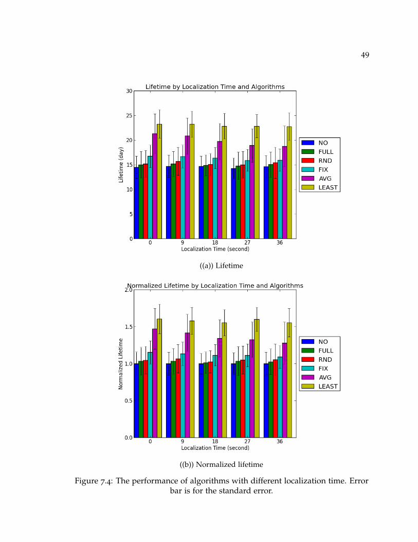
Fig. 7.4(a) shows lifetime of five charging algorithms on sensor network of
different localization time. The sensor network lifetime is supposed to be increased
as the localization time decreases, since the localization process consumes extra
energy. Fig. 7.4(b) shows the lifetime of each algorithm normalized around the base
case, no charge. For the LEAST algorithm, the improvement fluctuates between
50% and 60% for all lengths of localization time. For the AVG algorithm, its
improvement increases from about 30% to about 45% if no localization time is
required. For all the algorithms with no knowledge of the sensor node energy level,
we can see the trend that the sensor network life decreases with the increasing of
the localization time. However, the difference is insignificant except that the FIX
algorithm’s improvement increase from about 10% to about 15%.
Overall, the longer the localization time, the shorter the sensor network lifetime.
For algorithms, FULL, RND and LEAST, the impact of reduced localization time is
49
((a)) Lifetime
((b)) Normalized lifetime
Figure 7.4: The performance of algorithms with different localization time. Errorbar is for the standard error.
50
slight. This is because the FULL and RND algorithms spend all the energy on a
very few number of sensor nodes the UAV meets at the beginning, and the LEAST
algorithm is sophisticatedly designed to charge each sensor node at most once.
All these algorithm only require a few times of localization process. The FIX and
AVG algorithms are supposed to gain more benefit from the reduced localization
time, because these two algorithms require the UAV to visit and then localize each
sensor node multiple times.
7.6 Varying Energy Capacity of UAV
Energy capacity of UAV is one of the main constraints of the UAV power transfer
system. As the development of the UAV, the cargo capacity of UAV is increasing.
So, in the future, the UAV might be able to carry larger size battery, which has
larger energy capacity.
Currently, the UAV is using a battery of 25 WH energy, and we test what if the
UAV can have batteries of 50 WH, 100 WH and 200 WH energy. Fig. 7.5 shows
the results. The larger the UAV energy capacity, the longer the sensor network
lifetime, for most of the algorithms. The AVG algorithm is an exception. This is
reasonable because when the UAV energy capacity is large enough for the UAV to
charge every sensor node to the initial average energy level of the sensor network,
the AVG algorithm can barely benefit from a larger UAV energy capacity. For the
FIX and LEAST algorithms, the sensor network lifetime is constantly improved
when the UAV energy capacity increases from 25 WH to 200 WH. For the FULL
algorithm, the improvement is slight even if the battery energy capacity is 200 WH.
This is because the sensor network lifetime is determined by the sensor node with
the least power, and algorithm FULL may fully charge a few sensor nodes and then
51
((a)) Lifetime
((b)) Normalized lifetime
Figure 7.5: The performance of algorithms with different UAV energy capacity.Error bar is for the standard error.
52
leave others completely uncharged. When the UAV energy capacity is 200 WH,
the RND algorithm becomes the second best. We guess that statistically the RND
algorithm transfers more energy to sensor nodes with less energy compared with
the FIX algorithm, and at the same time it covers more sensor nodes compared
with the FULL algorithm.
7.7 Varying Energy Consumption Rate of UAV
Hovering
Because the UAV consumes a significant amount of energy for hovering while
charging a sensor node, we are interested in reducing the energy used for hovering
and exploring its influence. For example, in the case where a sensor node is placed
on the ground, the UAV can land on it and then turn off its motors.
Fig. 7.6 demonstrates the influence of zero hovering energy consumption rate.
As expected, the performance of all the algorithms are improved. The previous
experiments shows that the naive charging algorithms, FULL and RND, can rarely
prolong the lifetime of the sensor network. However, Fig. 7.6(a) shows that their
performance are significantly improved with zero hovering energy consumption
rate. The FULL algorithm can prolong the lifetime by about two days, and the RND
algorithm can prolong the lifetime by more than five days. To easily see the lifetime
percent gained, Fig. 7.6(b) shows the lifetime with no cost to hover normalized
around the lifetime with the standard energy consumption rate for each algorithm.
The LEAST algorithm gains largest percent, 60%, of improvement. After that,
charging algorithm RND gains about 40 percent improvement. Algorithms FIX
and AVG are both improved more than 30 percent as well.
53
((a)) Lifetime
((b)) Normalized lifetime
Figure 7.6: The performance of algorithms with different hovering energyconsumption rate. Error bar is for the standard error.
54
It is obvious that all the charging algorithms can greatly benefit from the
reduced energy consumption for hovering. This result suggest that, when charging
the sensor nodes, the UAV should land, when it is possible.
7.8 Varying Energy Consumption Rate of Wireless
Power Transfer
To charge a specific amount of energy to a sensor node, with a fixed charging
efficiency rate, the higher the transfer energy consumption rate, the shorter the
required time. Because the UAV consumes extra energy for hovering while
charging a sensor node, shorter charging time can reduce the extra energy for
hovering. We guess that the performance of the algorithms can be improved with
a higher transfer energy consumption rate.
Fig. 7.7 shows the performance of algorithms with different transfer energy
consumption rate. For algorithms with no knowledge of sensor node energy level,
FULL, RND and FIX, the gained benefit is very limited. For the algorithm with
some knowledge of sensor node energy level, AVG, the improvement is more
significant. For example, when the transfer energy consumption rate is 20 W, the
AVG algorithm prolongs the lifetime of the sensor network by about 25%, and
when the transfer energy consumption rate is 80 W, the AVG algorithm prolongs
the lifetime of the sensor network by about 60%. For the algorithm with complete
knowledge of sensor node energy level, LEAST, the improvement is also obvious.
The prolonging of lifetime increases from about 60% to almost 90% when the
transfer energy consumption rate changes from 20 W to 80 W.
55
((a)) Lifetime
((b)) Normalized lifetime
Figure 7.7: The performance of algorithms with different transfer energyconsumption rate. Error bar is for the standard error.
56
7.9 Varying Charging Efficiency Rate of Wireless
Power Transfer
Higher charging efficiency rate implies that same energy can be charged to the sen-
sor nodes with less time and energy consumption. We expect that the increment of
lifetime can be positively and significantly improved when doubling the efficiency.
However, our expectation is not true. Fig. 7.8 shows that the benefit of higher
charging efficiency is not obvious for algorithms, FULL, RND and FIX. The AVG
algorithm improves its performance when the charging efficiency rate increases
from 0.2 to 0.4, but the its performance almost does not change when the charging
efficiency rate increases from 0.4 to 0.6. We guess that it is because that the UAV
mainly spends the gained time (by reducing charging time) on looking for and
localizing more sensor nodes, instead of transferring more energy to visited sensor
nodes. This indicates that the algorithms should adjust their parameters based on
the state of the sensor network. For instance, with default system parameters 156 J
is nearly optimal for FIX algorithm, but with increased transfer efficiency 312 J
might be closer to the optimal value. Indeed, the LEAST algorithm, which is able
to adjust its charging schedule based on the available full knowledge, has the most
stable improvement with the increasing charging efficiency rate.
7.10 Comparison of System Parameters
In the previous sections, we have individually discussed the impacts of a series
of system parameters. In this section, we want to compare the impacts of these
system parameters to each other.
Fig. 7.9 shows the sensor network lifetime by system parameter changes for
57
((a)) Lifetime
((b)) Normalized lifetime
Figure 7.8: The performance of algorithms with different charging efficiency rate.Error bar is for the standard error.
58
((a)) Individual system parameter changes
((b)) Individual and combined system parameters changes
Figure 7.9: The performance of LEAST algorithm with different system parameterchanges.
59
LEAST algorithm. In this figure, label Basic means that default system parameters
are used, label Localization means that the localization time is changed to 0 second,
label Capacity means that the UAV energy capacity is changed to 200 WH, label
Hovering means that the UAV hovering energy consumption rate is changed 0 WH,
label Transfer means that the wireless power transfer energy consumption rate
is changed to 80 WH, label Efficiency means that the charging efficiency rate is
changed to 0.8, and label Combined means the combination all all these changes.
In Fig. 7.9(a), all the data match the data we presented in the previous sections.
The plot shows that decreasing the localization time from 36 seconds to 0 seconds
has little effect. The sensor network lifetime can be prolonged to almost 45 days
if the UAV can have 200 WH energy capacity. Even though the improvement is
significant, it is not likely to occur soon since 200 WH is 8 times larger than the
current 25 WH. Reducing hovering energy consumption rate can also greatly
improve the performance. In addition, it is more achievable since landing the
UAV while charging can reduce energy consumption of hovering. Both larger
wireless power transfer energy consumption rate and better charging efficiency
can mildly improve the performance. Larger energy transfer is likely since it is
obtainable with current system by using higher voltage batteries. Better charging
efficiency is also possible because Kurs et al. already experimentally measured
about 0.8 charging efficiency at a distance of 1m [17]. In fact, based on these
comparisons, we see that the UAV energy capacity is the most important (but hard
to achieve), and removing the hovering while charging is nearly as important but
much easier to achieve simply by landing while charging. Fig. 7.9(b) adds the data
of the combined changes. To demonstrate the idea we set the sensor node energy
capacity to unlimited otherwise the sensor network lifetime is bounded by the
sensor node energy capacity. Obviously we are still faraway from this, but it shows
60
us that the UAV only need to charge the sensor nodes once and then the sensor
network can work for more than one year.
7.11 Summary
These results show that the energy status of the sensor network can effectively
guide the behavior of UAV. We consider this, 8 sensor nodes distribute on a 200 m
× 200 m field, as the basic case. With no information of the energy level of sensor
nodes, the best charging algorithm can achieve about 15% improvement. With
information of the initial average energy of sensor nodes, the charging algorithm
can achieve about 40% improvement. With information of the energy level of each
sensor node, the algorithm can achieve about 60% improvement. In fact, for all the
system parameters we tested, the results show that the algorithm with complete
information always beats all the other algorithms, and the algorithm with some
information mostly beats all the algorithms with no information. Even more, in
some cases, the algorithm with complete information is the only algorithm which
can effectively prolong the lifetime the sensor network. For instance, when the
distance between UAV base station and the sensor network increases to 2000 m,
the LEAST algorithm can improve the sensor network lifetime by about 20%, and
the improvement by all the other algorithms can barely achieve 5%.
These results also imply that the majority of UAV’s energy is being spent
charging the nodes and hovering. Assuming as we do that the energy capacity of
a sensor node is 2.34 WH, and knowing that the UAV consumes 20 W to transfer
power with an efficiency rate of 0.2, the energy transferred to the node is 4 W.
At this rate, it would take 35 minutes to charge a fully discharged node. The
energy required to fully charge just one completely discharged node exceeds the
61
energy capacity of the UAV. If the UAV has a larger energy capacity, like 200 WH,
the sensor network lifetime can be improved to more than 40 days in the best
case. One experiment shows that a higher charging efficiency rate can improve
all the algorithms’ performance. For instance, the the sensor network lifetime is
improved to about 25 days by the AVG algorithm and to about 30 days by the
LEAST algorithm, when the charging efficiency rate is 0.8. Another experiment
shows that for the LEAST algorithm the prolonging of lifetime increases from
about 60% to nearly 90% when the energy consumption rate of transfer changes
from 20 W to 80 W. Additionally, the cost to hover is very expensive. The energy
consumption rate of hovering is 92.28 W and the efficient energy transfer is 4 W.
By that it means the UAV consumes 23.07 unit of energy for hovering to transfer
1 unit of energy to the sensor nodes. According to one experiment, if the UAV
does not have to hover while charging the sensor nodes, the LEAST algorithm can
prolong the sensor network lifetime from about 15 days to more than 35 days. In
addition, even the most naive algorithm, FULL, can prolong the sensor network
lifetime by 2 days in this case. The localization process is the overhead for the UAV
before charging a sensor node. An experiment shows that most algorithms can
only slightly benefit from a reduced localization time, even when the localization
time is 0 second. For instance, the AVG can prolong the sensor network lifetime
to about 19 days for a localization time of 36 seconds and to about 21 days for a
localization time of 0 second.
To summarize, we believe that reducing the energy consumption of UAV
hovering by landing the UAV while charging a sensor node is the most efficient
method to improve the performance of the UAV-based wireless power transfer
system. Also, the system can benefit from larger UAV energy capacity, more
efficient wireless power transfer and reduced localization time as well.
62
Chapter 8
Conclusions
In this work, we study the problem of how to use a UAV to effectively charge a
sensor network with wireless power transfer.
8.1 Contributions
The contributions of this work are as follows.
NP-Completeness Proof: The problem is based on a novel UAV-based wireless
power transfer system. We introduce the background of the problem, give a formal
definition of the problem, and also prove its NP-Completeness by reduction from
the problem Metric-TSP.
Heuristic Algorithms: As the problem is NP-Complete, we propose three cate-
gories of heuristic algorithms based on different information types, No Knowledge,
Some Knowledge and Complete Knowledge, of sensor node energy level. Experi-
ment results show that these algorithms can effectively prolong the lifetime of
a basic sensor network by 50%, and some advanced algorithms can significantly
outperform some naive algorithms.
63
Bottlenecks Identification: The experiment results indicate that the biggest
bottleneck of the current UAV-based wireless power transfer system is the huge
energy consumption of hovering while the UAV is charging sensor nodes. This
finding suggests us to make the UAV being able to land while charging in our next
generation of UAV-based wireless power transfer system. Also, we identify that
limited UAV energy capacity and inefficient wireless power transfer also notably
restrict the overall performance.
8.2 Future Work
The work presented is only a first step in investigating UAV-based wireless power
transfer system. There are several directions in which this work will proceed.
More Accurate Simulation: In the future, we can build a more accurate sim-
ulation system. For example, the current simulation system does not consider
the acceleration of moving. We just assume that the UAV can have immediate
stop and immediate optimal speed. Also, in real life the energy consumption rate
of then sensor nodes is changing since the sensor nodes work for a little while
and then rest for a while. However, the current simulation system consider the
sensor nodes have a constant energy consumption rate. In our next generation
of simulation system, we can remove all this type of assumptions and make the
simulation results more accurate.
Multiple UAVs: As we discussed, the UAV has a limited energy capacity, so it
is hard for a UAV to cover more than tens of sensor nodes in a single flight. As
the cost of the UAV is decreasing, more and more UAVs will be affordable. Then,
how to arrange multiple UAVs to work together and effectively charge tens or
hundreds of sensor nodes is a challenge. A naive solution is to assign a group of
64
sensor nodes to a UAV, and then every UAV only charge its assigned sensor nodes.
More advanced algorithms should make the UAV dynamically select sensor nodes
based on the status, such as location and energy level, of UAVs and sensor nodes
to optimize the performance.
Multiple Flights: In our work, we only consider the scenario where the UAV
can charge the sensor nodes with a single flight. In fact, the UAV might be able
to be recharged at the base station, and then the UAV can fly out and charge the
sensor nodes periodically. For charging with a single flight, the best strategy is to
charge those sensor nodes with low energy level because the UAV can only have
a single flight and the sensor network lifetime is determined by the sensor node
with lowest energy level. However, if the UAV is able to repeatably charge these
sensor nodes, the UAV might want to charge one single node as much as possible
for every flight to reduce the overhead of charging and then improve the overall
efficiency. We are interested in exploring this scenario in our future work.
65
Bibliography
[1] M.C. Achtelik, J. Stumpf, D. Gurdan, and K.-M. Doth. Design of a flexible high
performance quadcopter platform breaking the mav endurance record with
laser power beaming. In Intelligent Robots and Systems (IROS), 2011 IEEE/RSJ
International Conference on, pages 5166–5172, Sept 2011. 2.2
[2] Ian F Akyildiz and Mehmet Can Vuran. Wireless sensor networks, volume 4.
John Wiley & Sons, 2010. 1
[3] Hande Alemdar and Cem Ersoy. Wireless sensor networks for healthcare: A