Variability of zooplankton communities at Condorseamount and surrounding areas, Azores (NE Atlantic)

Vanda Carmo a,n, Mariana Santos b,c, Gui M. Menezes a, Clara M. Loureiro a,d,Paolo Lambardi a, Ana Martins a,d

a Departamento de Oceanografia e Pescas, Universidade dos Açores, Rua Professor Doutor Frederico Machado, 9901-862 Horta, Faial, Açores, Portugalb IMAR – Instituto do Mar, Centro do IMAR da Universidade dos Açores & Laboratorio Associado LARSyS, Rua Professor Doutor Frederico Machado, 9901-862Horta, Faial, Açores, Portugalc IPMA, Instituto Português do Mar e da Atmosfera, Av. de Brasília 6, 1449-006 Lisboa, Portugald CIBIO, Centro de Investigação em Biodiversidade e Recursos Genéticos, InBIO Laboratório Associado, Pólo dos Açores & Departamento de Oceanografia ePescas, Universidade dos Açores, Rua Professor Doutor Frederico Machado, 9901-862 Horta, Faial, Açores, Portugal

a r t i c l e i n f o

Available online 24 August 2013

Keywords:Zooplankton abundanceZooplankton biomassSeasonal variabilityCondor seamountAzores

a b s t r a c t

Seamounts are common topographic features around the Azores archipelago (NE Atlantic). Recently therehas been increasing research effort devoted to the ecology of these ecosystems. In the Azores, themesozooplankon is poorly studied, particularly in relation to these seafloor elevations. In this study,zooplankton communities in the Condor seamount area (Azores) were investigated during March, July andSeptember 2010. Samples were taken during both day and night with a Bongo net of 200 mm mesh thattowed obliquely within the first 100 m of the water column. Total abundance, biomass and chlorophyll aconcentrations did not vary with sampling site or within the diel cycle but significant seasonal variationwas observed. Moreover, zooplankton community composition showed the same strong seasonal patternregardless of spatial or daily variability. Despite seasonal differences, the zooplankton communitystructure remained similar for the duration of this study. Seasonal variability better explained our resultsthan mesoscale spatial variability. Spatial homogeneity is probably related with island proximity and localdynamics over Condor seamount. Zooplankton literature for the region is sparse, therefore a short reviewof the most important zooplankton studies from the Azores is also presented.

& 2013 Elsevier Ltd. All rights reserved.

1. Introduction

Seamounts are topographically distinct seafloor features thatoccur ubiquitously in the world's oceans but are still considered asone of the least known habitats on earth (Pitcher, 2007). In recentdecades, there has been considerable research effort focused onseamount ecology, as outlined in the reviews of Keating et al.(1987), Rogers (1994), Pitcher (2007), Clark et al. (2010) andSchlacher et al. (2010). A series of paradigms emerged based onearly seamount studies (Rowden et al., 2010a), suggesting sea-mounts as stepping stones for dispersal (Hubbs, 1959), places ofenhanced production (e.g. Dower et al., 1992; Genin and Boehlert,1985), biodiversity hotspots (e.g. Samadi et al., 2006; Worm et al.,2003) and ‘oases’ of increased abundance and biomass (Samadiet al., 2006), not only for fish (Morato and Clark, 2007) but also forinvertebrates (Rowden et al., 2010b). While it is generally acceptedthat increased vertical nutrient fluxes and material retention onseamounts may result in enhanced productivity and trophic uplift,

there is still little scientific proof of such phenomena. In fact,according to some authors (e.g. Mendonça et al., 2012; White et al.,2007), the variability between different seamounts and theirdissimilar local dynamics disrupt the above “idealized” model ofseamount ecology and the rather well established paradigms, sothese generalizations must be carefully applied (McClain, 2007;Schlacher et al., 2010).

In the upper layers of the open ocean zooplankton has a keyrole in the food web by establishing the link between primaryproduction and higher trophic levels, which include fish of com-mercial interest (Lenz, 2000; Raymont, 1983a). One of the hypoth-eses for explaining the trophic mechanisms at seamounts statesthat the vertically migrating zooplankters that during their descentabruptly encounter the seafloor in shoal areas become vulnerableto the resident predators (Isaacs and Schwarzlose, 1965). Theinteraction between the daily accumulation of zooplankton, pre-dation, physical advection and local dynamics can promote trophicfocusing and prey subsidy up the food web thus supportingaggregations of higher predators (Genin 2004; Genin and Dower,2007; Genin et al., 1994). Therefore, studying the abundance anddistribution of zooplankton and its trophic relations can bringfurther insight into seamount ecosystem functioning.

Contents lists available at ScienceDirect

journal homepage: www.elsevier.com/locate/dsr2

Deep-Sea Research II

0967-0645/$ - see front matter & 2013 Elsevier Ltd. All rights reserved.http://dx.doi.org/10.1016/j.dsr2.2013.08.007

n Corresponding author. Tel.: þ351 292 207 800; fax: þ351 292 207 811.E-mail addresses: vandacarmo@gmail.com, vandacarmo@uac.pt (V. Carmo).

Deep-Sea Research II 98 (2013) 63–74

Seamounts have been historically exploited by Azorean fisher-men due to their empirical knowledge of local fish aggregations(Brewin et al., 2007). Recent research at Azorean seamountsfocused mainly on fish and fisheries (Menezes et al., 2006, 2009;Morato et al., 2008; Pitcher et al., 2010; Porteiro and Sutton, 2007),while zooplankton has been largely overlooked. There are fewstudies on zooplankton from the Azores area and these are limitedto estimations of displacement volume (Dias et al., 1976; Sobralet al., 1985) and biomass (Sobrinho-Gonçalves and Isidro, 2001).Other investigations focused on mesozooplankton and copepodcommunity composition from areas nearby but away from Azoresregion (Gaard et al., 2008; Head et al., 2002; Huskin et al., 2004).Only two studies on seamounts located within the AzoreanExclusive Economic Zone (EEZ) were found, examining biomass(Martin and Christiansen, 2009; Sobrinho-Gonçalves and Cardigos,2006), size distribution and vertical migration data (Martin andChristiansen, 2009), but details on the taxonomic composition ofzooplankton main groups are missing. In this regard, the majorgoal of this study was to provide further knowledge about thezooplankton community in the archipelago of the Azores bydetermining its variability in terms of abundance, biomass andcomposition at the Condor seamount.

2. Material and methods

2.1. Study site

Condor seamount is located about 17 km southwest of FaialIsland, Azores. This seamount is 39 km long, 23 km wide, withdepths ranging from 2000 m and as little as 185 m at the mainsummit (Tempera et al., 2013). Condor is elongated in shape(mainly in an east–west direction), is nearly flat at a depth ofnearly 300 m, and bears two major peaks. This seamount isinhabited by cold water corals, sponges, sea-urchins, crabs, andseveral fish species of economical interest (Morato et al., 2010;Tempera et al., 2012). The study area and oceanographic contextare described in more detail in Bashmachnikov et al. (2013) andTempera et al. (2012, 2013). In the past, this seamount was heavilyfished by local fishermen (Menezes et al., 2013). The AzoresRegional Government has declared Condor seamount closed fordemersal/deep water fishing from 2010 to 2014, although scientificresearch and other uses (i.e. touristic activities) are still allowed(Giacomello et al., 2013).

2.2. Field sampling

The material for this study was provided by three cruisesaboard R/V Arquipélago. These occurred in March (“CONDOR-PAC-

MAR10”), July (“CONDOR-PAC-JUL10”) and September (“CONDOR-PAC-SET10”) 2010.

Previous studies from the Azores region (Martins et al., 2007),and more specifically for Condor seamount (Martins et al., 2011),showed that despite interannual variability in the region, seasonsare well defined in terms of near-surface chlorophyll a concentra-tions (as a proxy for phytoplankton), sea-surface temperature(SST), water stratification and mixing properties. Based on thesestudies, as well as phytoplankton average seasonal cycles for theregion (Santos et al., 2013), we defined seasons as: spring (March–May), summer (June–August), autumn (September–November),and winter (December–February).

The sampling sites selected for this work are shown in Fig. 1.Due to operational and financial limitations, only four stationswere sampled. Station CP11 corresponds to Condor seamountsummit; station CP03 is located in a deeper channel betweenCondor and Faial Island; station C01 is placed SE of Condorseamount, near Pico Island; and station C08 is located in deepestwaters NW of Condor. These locations were sampled once a month(i.e. March, July and September) during both day and nighttimeregimes within a 24 h period. Night sampling was performed inthe dark period between sunset and sunrise and daytime samplingafter sunrise and before sunset. A total of 20 samples were used inthis study. Equipment malfunctions or bad weather conditionsprevented sampling to be carried out in a few sites during certainperiods.

Sampling material included a Bongo net system with twoseparate nets (60 cm in diameter) of different mesh sizes(200 μm and 335 μm) each equipped with a collector, a digitalflow meter (Hydro-Bios, Model 438110), and a datalogger (VemcoMinilog TDR). Only zooplankton captured by the 200 μm mesh netwas used in this study. The upper 100 m of the water column wastowed obliquely, at a hauling speed of approximately 1 m s�1, forabout 20 min. The zooplankton collected in the cod-end bucketwas then preserved in a 1 l container with a solution of neutralizedformaldehyde (4%) and seawater. The volume of water filteredduring the haul was calculated based on the flow meter data,while real tow time was obtained from the datalogger record. Oneliter of surface seawater was also collected on each sampling sitefor in situ chlorophyll a concentration determination. Due to TDRmalfunctions at some stations, real time depth and temperaturewere not registered. Bottom depth was then calculated through anacoustic sounder EK500 and based on the average depths regis-tered at the start and end of the Bongo net tow. Ocean surfacetemperature was obtained by acquiring daily L2 MODIS/AQUA1 km resolution satellite data obtained from the Ocean Color Level1/2 browser (OceanColor Web, 2006). These images were mapped(Level2-map) with SeaDAS (NASA/GSFC), by creating a master filespecifically for the Condor region. The download and mapping

Fig. 1. Study area and location of zooplankton sampling sites. Numbers beneath the station codes represent the average bottom depth of all oblique tows at that station.

V. Carmo et al. / Deep-Sea Research II 98 (2013) 63–7464

Table 1Sampling details including environmental data and zooplankton abundance/biomass results for each sample. Sample code, station code as in Fig. 1; D/N, day or night sample; M/J/S, month of sampling: March, July or September.Chl, chlorophyll. Biovolume¼zooplankton displacement volume/volume water filtered.

Samplecode

Date LatitudeN (in)

LongitudeW (in)

LatitudeN (out)

LongitudeW (out)

Averagebottomdepth (m)

Chl a in situ(mg m�3)

Chl aMODIS(mg m�3)

SurfaceTemperatureMODIS (1C)

Volumewaterfiltered(m�3)

Biovolume(ml m�3)

Totalabundance(no 103 m�3)

Biomass(mg DW m�3)

C01N_M 30-03-2010 38125′85″ 28128′78″ 38125′42″ 28129′21″ 359.1 0.486 1.149 15.5 221.973 0.189 0.77 19.7C08N_M 31-03-2010 38134′30″ 29118′19″ 38133′92″ 29117′81″ 1883.7 0.822 1.149 15.5 271.052 0.192 1.43 20.0CP03D_M 30-03-2010 38131′79″ 28150′59″ 38131′99″ 28151′07″ 978.7 0.768 1.149 15.5 104.875 0.420 3.29 49.4CP03N_M 29-03-2010 38131′75″ 28150′65″ 38132′02″ 28151′49″ 989.8 0.249 0.25 14.8 266.946 0.322 1.86 36.4CP11D_M 30-03-2010 38132′35″ 29102′74″ 38132′00″ 29103′04″ 260.3 0.186 1.149 15.5 228.598 0.096 1.00 9.0CP11N_M 30-03-2010 38132′36″ 29102′58″ 38131′55″ 29102′76″ 297.0 0.178 1.149 15.5 272.731 0.125 1.18 12.1C01D_J 08-07-2010 38125′84″ 28128′73″ 38125′38″ 28128′92″ 351.6 0.081 0.074 21.5 70.166 0.399 2.64 46.6C08D_J 06-07-2010 38134′25″ 29118′06″ 38134′05″ 29117′38″ 1877.8 0.021 0.074 21.5 211.523 0.104 1.17 9.8CP03D_J 08-07-2010 38131′74″ 28150′76″ 38132′02″ 28151′31″ 988.8 0.049 0.074 21.5 59.156 0.338 2.58 38.5CP03N_J 09-07-2010 38131′67″ 28150′78″ 38131′44″ 28151′32″ 906.1 0.014 0.074 21.5 74.738 0.428 2.19 50.5CP11D_J 10-07-2010 38132′34″ 29102′78″ 38131′85″ 29102′25″ 210.6 0.164 0.074 21.5 78.563 0.331 2.03 37.5CP11N_J 10-07-2010 38132′33″ 29102′76″ 38131′84″ 29102′83″ 290.0 0.007 0.074 21.5 71.938 0.139 1.23 13.8C01D_S 17-09-2010 38125′77″ 28128′75″ 38125′23″ 28129′14″ 398.0 0.008 0.063 22.9 210.124 0.057 0.53 4.9C01N_S 17-09-2010 38125′83″ 28128′76″ 38125′30″ 28129′32″ 378.5 0.004 0.063 22.9 184.371 0.130 0.43 12.8C08D_S 15-09-2010 38134′24″ 29118′08″ 38133′88″ 29117′52″ 1875.8 0.011 0.063 22.9 273.664 0.110 0.52 10.5C08N_S 18-09-2010 38134′32″ 29118′35″ 38134′01″ 29117′96″ 1879.5 0.004 0.063 22.9 156.286 0.128 0.80 12.5CP03D_S 18-09-2010 38131′65″ 28150′68″ 38131′23″ 28151′12″ 873.6 0.029 0.063 22.9 160.112 0.050 0.41 4.2CP03N_S 18-09-2010 38131′64″ 28150′61″ 38131′35″ 28151′40″ 867.0 0.017 0.063 22.9 202.379 0.109 0.58 10.4CP11D_S 17-09-2010 38132′29″ 29102′62″ 38131′76″ 29102′84″ 319.2 0.006 0.063 22.9 132.307 0.106 0.83 10.0CP11N_S 17-09-2010 38132′37″ 29102′69″ 38131′69″ 29102′68″ 300.0 0.003 0.063 22.9 110.660 0.163 1.17 16.5

Missing samples: C01D_M, C08D_M, C01N_J, C08N_J (no sampling occurred due to bad weather conditions or equipment malfunctions).

V.Carmoet

al./Deep-Sea

Research

II98

(2013)63

–7465

process was automated within the HAZO system developed byFigueiredo et al. (2004). Weekly (8-day) averages were derived foreach location and period. MODIS also provided near-surfacechlorophyll a concentration data for the same time and region.

2.3. Laboratory procedure

Biomass was estimated by measuring the total displacementvolume (DV, ml) of each sample. Plankton was filtered andseparated from its preserving fluid with a small 200 μm net (witha volume of 2 ml) and then completely immersed inside ameasuring cylinder of 250 ml (72 ml) containing a knownamount of the preserving liquid. The DV was obtained by thedifference between the final measurement (subtracting the netvolume) and the original volume in the measuring cylinder. TheDV was then converted to dry weight (DW, mg m�3) using theregression calculated by Wiebe (1988)

log ðDVÞ ¼ �1:842þ0:865 log ðDWÞEvery 1 l sample was then sub-sampled for observation using a

Folsom Splitter. Fractions of 1/256 and 1/16 from each samplewere usually applied, but these depended on the abundance oforganisms, i.e. in rarefied samples the 1/128 and 1/8 divisionswere used instead. Individual organisms were counted andidentified in a zooplankton chamber to the lowest possibletaxonomical level, given the timeline and objective of this study,using a stereoscope (Leica MZ16FA) coupled with an imagerysystem. All individuals of the 1/256 fraction were counted so thatthe total was at least 400 individuals (Stehle et al., 2007). In casethe total count was less than 400, the analyzed sub-sample wasdoubled to 1/128. In the small sub-sample, all taxa accounted forZ50 individuals were directly extrapolated for the total. Only lessabundant and rare taxa (o50 individuals) were then (re)countedon the larger fraction (1/16 or 1/8). Abundance per taxon and totalabundance (no. m�3) were estimated based on the volume ofseawater filtered in each tow.

For chlorophyll a concentration determination, 1 l of surfaceseawater was vacuum-filtered on 47 mm Whatman grade GF/Fglass microfiber filter and then stored in a �80 1C freezer. Thesubsequent analysis followed the recommendation of Yentsch andMenzel (1963), based on the “Turner Fluorometer” method, andwas described in detail in Arístegui et al. (2009). Chlorophyll aconcentration was determined using the LS 55 FluorescenceSpectrometer.

2.4. Statistical analysis

Univariate analyses were executed using the software packageSTATISTICA 6.0 while multivariate analyses were performed onPRIMER 6 (Clarke and Gorley, 2006) with the add-on PERMANOVAþ(Anderson et al., 2008).

A PERMANOVA (Permutational Multivariate Analysis ofVariance) with three factors, crossed and fixed, was employed tocompare zooplankton total abundance and biomass among sea-sons (sampling months), locations (stations) and diel migrations(day/night samples), followed by pairwise tests whenever appro-priate. For these analyses, variables were standardized by theirtotal and for the resemblance matrix the Euclidean distance wasapplied.

A series of analyses were then performed to investigate themain patterns of the zooplankton community composition andtaxonomic diversity. The raw matrix of zooplankton abundances atthe lowest possible taxonomic level for each sample was squareroot transformed. The Bray–Curtis resemblance measure wasapplied for the remaining multivariate analyses. A dominance plotwas used to investigate changes in diversity and evenness in each

sampling period. Data were averaged per sampling month only forthe dominance plot. A PERMANOVA test was also applied to adistance-based matrix of the monthly dominance curves (obtainedby the DOMDIS routine, log-weighting taxa ranks) to test forseasonal sampling period differences in zooplankton diversity.Ordination by Principal Coordinates Analysis (PCO) was used toidentify groups of samples and patterns in zooplankton commu-nity composition, followed by the Similarity Percentage (SIMPER)routine for determining which taxa most contributed to thedifferences obtained among the identified groups. PERMANOVAroutines tested formally for differences in zooplankton communitycomposition between seasons (sampling months), locations (sta-tions) and diel migrations (day/night samples).

3. Results

3.1. Total zooplankton biomass and abundance, and chlorophyll aconcentration

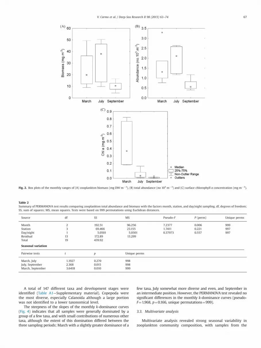
Table 1 provides detailed information about every sample usedin the present study and Fig. 2 summarizes some of these resultswithin each sampling period. Zooplankton biomass estimateswere highest on an average in July (�32.8 mg DW m�3) andlowest in September (�10.2 mg DW m�3). Zooplankton totalabundance was similar between March and July and much lowerin September, with an average of �1300 individuals per m3 in allperiods sampled. The in situ chlorophyll a concentration averagewas 0.155 (standard error¼0.056 mg m�3) while MODIS estimateswere more than twice this estimate (0.347 mg m�3). SST valueswere more conservative within each sampling period, due in partto the influence of occasional high cloud cover on the 8-dayaverage, but show seasonal variability as expected for the region,varying between �15 and 23 1C.

We tested zooplankton total abundance and biomass in relationto sampling site or diel period and the results showed nosignificant differences (Table 2). Nevertheless, significant differ-ences were obtained between sampling months, with Septembersamples significantly different from the others.

3.2. Zooplankton composition and taxonomical diversity

In terms of zooplankton groups across all samples, Crustaceadominated comprising 72.6% of total abundance, mainly repre-sented by Copepoda (60.9%). Urochordata was another importantgroup (17.4%), followed by Protozoa (4.7%) and Mollusca (3.5%).Other taxa merely represented 1.9% of total abundance.

In terms of seasonal zooplankton composition (Fig. 3), Calanoidcopepods dominated the samples in all months studied, althoughthis group had much higher relative abundances in March (57.8%)and September (45.8%) than in July when they were reduced bynearly half (26.5%). The second position, in terms of relativeabundance, fluctuated between Crustacea nauplii in early spring(12.5%), Appendicularia in summer (18.0%) and Cyclopoida in latesummer (13.3%). The copepod groups, Poecilostomatoida andCyclopoida, alternated between second and fifth positions butwere always important in terms of abundance, each representingabout 10% of the monthly total. An exception occurred in March,when the Poecilostomatoida (11.1%) were twice as abundant asCyclopoida (5.6%), while in the other two months Cyclopoida wereslightly more abundant. In July, the relative abundances of eachtaxon were slightly more even than in other sampling periods,Appendicularia and Doliolida having the greatest abundanceof all months sampled (together almost 30%), and groups such asCladocera (5.6%) and Cirripedia larvae (3.7%) appearing amongstthe top 10.

V. Carmo et al. / Deep-Sea Research II 98 (2013) 63–7466

A total of 147 different taxa and development stages wereidentified (Table A1—Supplementary material). Copepoda werethe most diverse, especially Calanoida although a large portionwas not identified to a lower taxonomical level.

The steepness of the slopes of the monthly k-dominance curves(Fig. 4) indicates that all samples were generally dominated by agroup of a few taxa, and with small contributions of numerous othertaxa, although the extent of this domination differed between thethree sampling periods; March with a slightly greater dominance of a

few taxa, July somewhat more diverse and even, and September inan intermediate position. However, the PERMANOVA test revealed nosignificant differences in the monthly k-dominance curves (pseudo-F¼1.968, p¼0.166, unique permutations¼999).

3.3. Multivariate analysis

Multivariate analysis revealed strong seasonal variability inzooplankton community composition, with samples from the

Fig. 2. Box plots of the monthly ranges of (A) zooplankton biomass (mg DWm�3), (B) total abundance (no 103 m�3) and (C) surface chlorophyll a concentration (mg m�3).

Table 2Summary of PERMANOVA test results comparing zooplankton total abundance and biomass with the factors month, station, and day/night sampling. df, degrees of freedom;SS, sum of squares; MS, mean squares. Tests were based on 999 permutations using Euclidean distances.

Source df SS MS Pseudo-F P (perm) Unique perms

Month 2 192.51 96.256 7.2377 0.006 999Station 3 69.466 23.155 1.7411 0.221 997Day/night 1 5.0501 5.0501 0.37973 0.557 997Residual 13 172.89 13.299Total 19 439.92

Seasonal variation

Pairwise tests t p Unique perms

March, July 1.1927 0.270 998July, September 2.368 0.015 998March, September 3.6418 0.010 999

V. Carmo et al. / Deep-Sea Research II 98 (2013) 63–74 67

same month grouping together but being clearly separated fromthe samples belonging to other months (Fig. 5). About 33% of thespecies composition variability is explained by the first PCO axis

that distinguishes well between samples taken in September andthose from other sampling periods. The second axis explains about23% of the variation, nicely separating the samples obtained inMarch and July. No clear patterns were detected for spatial(stations) or diel migration (day/night) differences, although therewas some segregation of the samples taken within the sameseason (e.g. station CP03 is somehow distinct from the remaindersampled in March, and stations CP11 and C08 are separated fromeach other and from the remaining stations in September).

Results of the SIMPER analysis revealed the most importanttaxa that contributed to discriminate the monthly groups obtainedby the PCO analyses (Table 3). In March, the Calanoida, namelythe group ‘Calanus spp. and Clauso-, Cteno-, Pseudo- and Para-calanus spp.’, Pleuromamma spp., the Poecilostomatoida Oncaeidaeand crustacean nauplii were more abundant than in the othermonths. In July, Appendicularia, Doliolida, the Copepoda Centro-pages spp. and Oithona spp., the Cladocera Evadne spp. andPseudevadne spp. and Cirripedia larvae dominated in relation toother periods. September was generally characterized by much

Fig. 4. Dominance plot representing the average k-dominance curves for eachmonth in the study.

Fig. 5. Principal coordinates analysis (PCO) plot based on Bray–Curtis similarity ofsquare root transformed abundances of zooplankton identified at the lowesttaxonomic level. Circles represent 60% of similarity.

OstracodaCalanoida

Crustacea nauplii Chaetognatha

CladoceraPoecilostomatoida

BivalviaCyclopoida

RadiolariaAppendicularia

CirripediaDoliolida

ForaminiferaEuphausiacea

OthersHydrozoa

57.8%

12.5%

11.1%

5.6%

4.6%2.1%

1.8%

0.9%

0.7%0.6%2.2%

March

26.5%

18.0%

10.8%

9.3%

9.0%

5.6%

5.0%5.0%3.7%

1.9%5.1%

July

45.8%

13.3%

12.9%

7.9%

7.5%

2.9%

1.9%1.0%1.0%0.9%

5.0%

September

Fig. 3. Monthly abundances (%) of the main zooplankton taxa (top 10).

V. Carmo et al. / Deep-Sea Research II 98 (2013) 63–7468

Table 3Most important taxa that determined the groups obtained in the PCO analysis. The average monthly abundances (no m-3, square root transformed), respective contributions (%),and the cumulative contributions (%) of each taxon to the observed dissimilarity between groups are provided.

SIMPER average dissimilarity¼42.94 SIMPER average dissimilarity¼44.76 SIMPER average dissimilarity¼43.43

Taxon Square root of abundance(no. m�3)

Taxon Square root of abundance(no. m�3)

Taxon Square root of abundance(no. m�3)

March July Contrib.%

Cumul.%

July September Contrib.%

Cumul.%

March September Contrib.%

Cumul.%

Appendicularia 7.85 17.79 6.1 6.1 Doliolida 13.99 1.95 8.12 8.12 Calanus spp.groupa

17.63 4.22 10.33 10.33

Centropagesspp.

0.54 10.04 5.55 11.66 Appendicularia 17.79 6.96 7.10 15.22 Crustaceanauplius

9.78 1.38 6.02 16.36

Doliolida 5.20 13.99 5.34 17.00 Centropagesspp.

10.04 1.18 5.84 21.06 Calanoida 17.17 11.82 5.51 21.87

Evadne spp. 0.00 7.51 4.57 21.57 Calanus spp.groupa

10.88 4.22 4.82 25.89 Oncaeidae 11.61 6.63 4.32 26.19

Calanus spp.groupa

17.63 10.88 4.29 25.86 Evadne spp. 7.51 1.79 3.92 29.81 Acantharia 0.94 5.94 3.92 30.11

Calanoida 17.17 10.98 4.10 29.96 Pseudevadnespp.

6.01 0.66 3.67 33.48 Pleuromamma spp. 5.34 1.39 3.34 33.45

Crustaceanauplius

9.78 4.87 3.90 33.86 Calanoida 10.98 11.82 3.19 36.67 Lucicutia spp. 5.67 2.12 2.92 36.38

Pseudevadnespp.

0.00 6.01 3.66 37.52 Cirripedianauplius

5.73 2.14 3.16 39.82 Doliolida 5.20 1.95 2.85 39.22

Cirripedianauplius

0.24 5.73 3.13 40.65 BivalviaVeligera larva

6.69 2.31 3.09 42.91 Eucalanidae 9.16 6.34 2.67 41.90

BivalviaVeligeralarva

1.71 6.69 2.87 43.52 Oithona spp. 13.18 9.28 2.81 45.72 Furcilia larva 3.43 0.37 2.37 44.26

Oithona spp. 9.14 13.18 2.73 46.25 Oncaeidae 10.15 6.63 2.80 48.52 Appendicularia 7.85 6.96 2.34 46.61Radiolaria 1.95 5.89 2.55 48.80 Radiolaria 5.89 2.58 2.63 51.14 Rhincalanus spp.

nauplius3.62 0.56 2.32 48.93

Pleuromammaspp.

5.34 1.56 2.43 51.22 Acartia spp. 6.29 4.52 2.29 51.21

a Calanus spp. and Clauso/Cteno/Pseudo/Paracalanus spp.

Table 4Summary of the results of PERMANOVA tests on zooplankton community composition for the factors month, station and day/night sample. Number of permutationsused¼9999.

Seasonal variation

Source df SS MS Pseudo-F P (perm) Unique perms Components of variation

Estimate Square root

Month 2 7817.1 3908.6 8.6545 0.0001 9936 523.78 22.886Residual 17 7677.5 451.62 451.62 21.251Total 19 15,495

Pairwise tests t p Unique perms

March, July 2.8094 0.0024 462July, September 2.9887 0.0005 2904March, September 3.0006 0.0005 2894

Spatial variation

Source df SS MS Pseudo-F P (perm) Unique perms Components of variation

Estimate Square root

Station 3 2174.7 724.9 0.87076 0.614 9915 �21.81 �4.6701Residual 16 13,320 832.5 832.5 28.853Total 19 15,495

Diel variation

Source df SS MS Pseudo-F P (perm) Unique perms Components of variation

Estimate Square root

Day/night 1 807.4 807.4 0.98951 0.3981 9451 �0.85569 �0.92504Residual 18 14,687 815.96 815.96 28.565Total 19 15,495

V. Carmo et al. / Deep-Sea Research II 98 (2013) 63–74 69

lower abundances of these taxa than in other months, with theexception of the Acantharia.

The PERMANOVA routine tested formally for differences inzooplankton taxonomical composition regarding three factors:season, location and day/night samples (Table 4). Spatial and dielvariation were not statistically significant, but again, there was ahighly significant monthly variation in the composition of theidentified zooplankters. Pairwise tests also revealed significantstatistical differences between the three months studied (July andMarch with po0.01 and September against the other two monthswith po0.001).

4. Discussion

4.1. Sources of bias

Variability in zooplankton estimates between previous studiesand ours (Table 5) can be related to environmental factors(including interannual variability) as well as sampling conditionsand methodology employed, such as sampling depth, gear, typeand duration of tows and mesh size. Even at comparable samplingdepths, the type and duration of tows may influence the catches,since vertical hauls sample a lesser distance, and consequently

Table 5Mesozooplankton biomass estimates for the Azores archipelago and surrounding areas in the NE Atlantic. See text for further details. D/N, day and/or night samples.

Study Area Sampling method Period of study Biomass estimates

Azores Archipelago and Seamounts (within 371–401N, 24–301W)Dias et al. (1976) Archipelago and seamounts Bongo net: 500 mm;

200–0 m; D/NNovember 1975 1.13 mg DW m�3a (average all

stations)Sobral et al. (1985) Archipelago and seamounts WP-2 net: 200 mm;

200–0 m; D/NSeptember 1979 34.17 mg DWm�3 (average all

stations)Muzavor (1981) Transect between Princesa Alice Seamount and S. Miguel

IslandNeuston–Schlitten:330 mm; sub-surface; D/N

March-April1980

23.04 mg DW.m�3b

Roden, 1987 Porto Pim Bay, S coast of Faial Island FAO net: 330 mm; sub-surface; N

September 1989–August 1990

11.68 mg DWm�3a (one yearaverage)

Silva (2000) Off the S coast of Faial Island Bongo net: 335 mm;100–0 m; N

February 1998 11.05 mg DWm�3a

March 1998 14.11 mg DWm�3a

May 1998 58.65 mg DWm�3a

June 1998 11.61 mg DWm�3a

July 1998 10.72 mg DWm�3a

August 1998 8.43 mg DWm�3(a)

Sobrinho-Gonçalvesand Isidro (2001)

Off the S coast of Faial Island Bongo net: 335 mm;100–0 m; N

February 1998 5.70 mg DWm�3a

March 1998 7.28 mg DWm�3a

May 1998 30.25 mg DWm�3a

June 1998 5.99 mg DWm�3a

Sobrinho-Gonçalvesand Cardigos (2006)

D. João de Castro seamount (38113′N, 26136′W) Bongo net: 335 mm;100–0 m; N

August 2000 2.00 mg DWm�3 (minimum, aboveseamount summit)6.00 mg DWm�3 (maximum, 3, 5 Nmiles away from summit)3.75 mg DWm�3 (average allstations)

Santos (2011) Off the W coast of Faial Island (Condor seamount) and SWof Pico Island

Bongo net: 200 mm;100–0 m; D/N

March 2009 26.53 mg DWm�3a

June 2009 17.83 mg DWm�3a

August 2009 14.62 mg DWm�3a

November 2009 9.61 mg DW m�3a

All periods 17.15 mg DWm�3a

Present study Off the W coast of Faial Island (Condor seamount) and SWof Pico Island

Bongo net: 200 mm;100–0 m; D/N

March 2010 24.42 mg DWm�3a

July 2010 32.78 mg DWm�3a

September 2010 10.22 mg DWm�3a

All periods 21.85 mg DW m�3a (average allstations)

Vicinity of the Azores, NE Atlantic

Angel (1989) Vicinity of the Azores Front, SW of the Azores (30–351N,30–341W)

RMT: 320 mm; 100–0 m; N November 1980 �3.20 mg DWm�3a (standingcrop)

RMT: 320 mm; 100–0 m; D April–May 1981 �4.00 to �7.00 mg DWm�3a

RMT: 320 mm; 100–0 m; N �8.00 to �23.00 mg DWm�3a

Gallienne et al. (2001) Transect 60�371N (centered at 201W) WP-2 net: 200 mm;200–0 m; D/N

July 1996 �1.00–4.00 mg DWm�3a

Head et al. (2002) Azores Current, transect between Azores and Madeira/Canary Islands (27158″–381N, 20136″–231W)

WP-2 net: 200 mm;200–0 m; D/N

August 1998 � 5.43 mg DWm�3c

April 1999 � 6.00 mg DWm�3c

Martin andChristiansen (2009)

Seine (33150′N, 14120'W), Sedlod (40120′N, 27150′W) andAmpère (35102′N, 12154′W) seamounts

MOCNESS: 333 mm;100–0 m; N

Autumn 2003 �8.00 mg DWm�3b (aboveseamount summit)�16.00 mg DWm�3b (seamountslopes and far-field)

MOCNESS: 333 mm;100–0 m; D

�10.00 mg DWm�3b (all stations)

MOCNESS: 333 mm;100–0 m; D

Summer 2004 �1.00 mg DWm�3b (aboveseamount summit)�5.00 mg DWm�3b (far-field)

a Converted from displacement volume after Wiebe (1988): log(DV)¼�1.842þ0.865 log(DW).b Converted from wet weight after Wiebe (1988): log(WW)¼�2.002þ0.950 log(DW).c Converted from carbon values after Wiebe (1988): log(DW)¼0.499þ0.991 log(C).d Only data for Sedlo (located N of the Azores archipelago but within its EEZ) is shown.

V. Carmo et al. / Deep-Sea Research II 98 (2013) 63–7470

volume of water, collecting far less plankton when compared withoblique hauls (Smith et al., 1985). Also, in theory, longer tows havea higher probability of encountering a zooplankton patch (Cassie,1968).

Regarding mesh size, Gallienne and Robins (2001) showed thatan important fraction of mesozooplankton between 200 and800 mm could be significantly under-represented, especially dueto the loss of smaller taxa and copepodite stages of largercopepods, which can have severe consequences on biomass andabundance estimates. A net with a 200 mm mesh, like the one usedin the present study, may capture less than 10% of the mesozoo-plankton total numbers and underestimate their biomass by one-third. Losses are even more dramatic in case 330 mm mesh nets areapplied. For example, Silva (2000) used the same gear andsampling methodology as in our study, excepting for mesh size(335 mm), and their total abundance estimates varied between ca.100 and 450 no. m�3, one order of magnitude less than ours.

Moreover, displacement volume (DV) as a measure for estimat-ing biomass can be quite inaccurate and cause great variabilityespecially when measured from fixed samples. Fixation informaldehyde (4%) can cause important losses of the live volumeof organisms, decreasing it between 15 and 82% (Ahlstrom andThrailkill, 1962). Thus, DV's measured after preservation under-estimate those of living material. According to the results ofAhlstrom and Thrailkill (1962), the decrease was greatest whengelatinous organisms made up most of the volume, while thesamples dominated by crustaceans had the smallest losses. In theirsamples the major volume losses up to 82% occurred immediatelyafter preservation, while afterwards the decrease did not varymuch (0–7% between 1 and 12 months). In our study, DV's weredetermined in October 2010 which corresponds to a period of 7,3 and 1 month of preservation since collection of the samples inMarch, July and September, correspondingly. In spite of thedifferences in preservation time, major volume losses should havealready occurred and samples should be comparable. Even thoughthe taxa were accounted for in terms of numbers (abundance) andnot by volume in this study, the gelatinous components were mostabundant in July, so any resulting underestimate should be mostpronounced in that month. Yet, the biomass estimate reached itsmaximum in summer. While our general results may be under-estimated they should not stray very far from the general trendthat would be expected if estimates had been determined from theDV of live animals.

4.2. Temporal and spatial variability in abundance and biomass

In the present study, total zooplankton abundance and biomassvaried seasonally, regardless of sampling site and daily cycle. Ourdata showed higher zooplankton abundance and biomass inMarch and July (spring/summer), compared with September (earlyautumn). Chlorophyll a concentration was reduced from the firstto the third sampling periods as expected for this region (Martinset al., 2007). Santos et al. (2013) also found a decreasing trend inchlorophyll a concentration (concerning the deep chlorophyllmaximum) at Condor seamount during the same year. Thisvariation is consistent with the relatively strong phytoplanktonbloom which occurred in spring 2010, starting in March andattaining its maximum in April, preceded by weak winter mixing,according to the results obtained by Martins et al. (2011) fromMODIS/AQUA near-surface derived monthly chlorophyll a concen-tration averages.

In March (late winter/early spring), the water column was wellmixed, temperature was still low but the phytoplankton bloomwas already underway (Santos et al., 2013). Therefore, we can inferthat the phytoplankton bloom was later followed by the growth ofthe zooplankton community that only peaked around

summertime. In July, water was stratified and warm (Santoset al., 2013), characteristic of the summer period, and the abun-dant zooplankton would have already consumed a large portion ofthe phytoplankton, leaving very low concentrations of chlorophylla in near-surface waters. Chlorophyll a was even more depleted inSeptember and, consequently, a diminished zooplankton commu-nity was observed during that same period most probably due tothe lack of food.

In contrast with 2010, strong winter mixing during 2009 likelycaused the phytoplankton to be distributed deeper in the watercolumn where photosynthesis is limited by the lack of sunlight.The phytoplankton bloom was therefore weakened and delayed,only occurring in May (Martins et al., 2011), which certainly hadconsequences in the zooplankton cycle that year. In fact, in 2009,the average zooplankton biomass in this location was much lowerin the summer period as found by Santos (2011) in the firstzooplankton investigations in the Condor area, when comparedwith summer 2010 (Table 5). These results are corroborated bystatistical analyses of nine years of 1.1 km resolution chlorophyll aand SST MODIS/AQUA satellite data processed for the Condorregion (Martins et al., 2011). This study showed that the springbloom was most dominant in April (0.39 mg m�3), and that,throughout the nine year period, spring blooms always occurredduring March, April or May and lowest chlorophyll a concentra-tions were found from July to September.

Other studies reported that zooplankton peaks in July 1990(Roden, 1987) in Porto Pim Bay (southern shore of Faial), and inMay 1998 off the southern coast of Faial island (Silva, 2000;Sobrinho-Gonçalves and Isidro, 2001). All these data follow theclassic annual productivity cycles for the region and the temperateNorth Atlantic, typical of mid-latitude ecosystems (Mann andLazier, 2006; Miller, 2004; Winder and Cloern, 2010).

Our zooplankton biomass estimates are in general agreementwith previous results for the same seasons of sampling in theregion (Table 5). Other studies conducted in the vicinity of theAzores (Angel, 1989; Gallienne et al., 2001; Head et al., 2002)presented biomass estimates lower by one order of magnitudewhen compared to the ones within the archipelago, with onlya few exceptions. In general, mesozooplankton biomass andabundance estimates throughout the region were low, character-istic of oligotrophic waters, and significant increases were onlyobserved in the Azores Subtropical Front (Huskin et al., 2001).

Only two studies were found in the Azores area that focusedspecifically on zooplankton at seamounts (Martin and Christiansen,2009; Sobrinho-Gonçalves and Cardigos, 2006). Martin andChristiansen (2009) found reduced zooplankton biomasses abovethe summits of Sedlo, Seine and Ampère seamounts (NE Atlantic),when compared to the slope and far-field stations, regardless oftime of day, season and summit elevation, possibly caused byhydrographic effects and predation. Sobrinho-Gonçalves andCardigos (2006) reported a mesozooplankton biomass hole abovethe summit of Dom João de Castro Seamount (Azores archipelago)when compared with the surrounding areas up to 4.3 nauticalmiles away. Both studies suggest a “seamount effect” to explaintheir data. Their biomass estimates were lower than the onesobtained for Condor, but this could have been a sampling artifact,due to the different mesh sizes employed. Our results did notreveal significant spatial variability, but must be interpreted withcaution since more stations and a different sampling designstrategy would have been necessary in order to fully understandspatial differences and a possible seamount effect.

No diel variations in mesozooplankton total abundance andbiomass were recognized in our data. Huskin et al. (2001) didnot find any differences related with daily cycles in copepodabundances in the first 200 m of the water column of theAzores Current. However, Martin and Christiansen (2009)

V. Carmo et al. / Deep-Sea Research II 98 (2013) 63–74 71

analyzed depth-stratified samples down to �4000 m, anddetected diel vertical migrations, in zooplankters (5–20 mm inlength/size) at Sedlo, Seine and Ampère seamounts. It is importantto bear in mind that in our study only the surface 100 m of thewater column were sampled. Discrete depth sampling down to theplateau and slopes would have to be employed to better explorethis subject.

During 2010, the summit circulation at Condor seamount wascharacterized most of the time by the presence of an “anticycloniccap or Taylor cap” given the weak impinging flow and strong waterstratification (see Bashmachnikov et al., 2013, for a detailedexplanation). While “Taylor columns” can extend all the way tothe sea-surface, in the case of Condor seamount, only a thin capwas formed over the summit and permanent trapping was justreported up to 50–60 m above the bottom. This is due to theimpinging flow being quite weak (below 10 cm s�1 90% of timeand below 5 cm s�1 40–50% of time) and stable, reaching at least600 m depth (Bashmachnikov et al., 2013). These authors alsoreported strongly intensified near-bottom mixing, in particularover the gentle eastern slope of Condor, but the vertical extensionof the trapped water volume was limited to the 200 m bottom-most layer, an effect that was not captured at our sampling depths.In this sense, stations and depth sampling procedures in thepresent study did not suffice for local patchiness to be detectedin the surface 100 m above and away from the seamount.

In the particular case of Condor, the proximity of Faial Island maycreate a “shadow effect” over the seamount causing instability andaffecting mean dynamics. In other words, the presence of the islandsas a topographic and ecosystem-conditioning feature (providingexogenous nutrients to the surrounding waters) at a medium spatialscale should influence the zooplankton community more stronglythan the presence of the moderately sized seamount itself.

4.3. Zooplankton community composition and taxonomical diversity

Multivariate analysis focused on the zooplankton communitycomposition supported our previous results regarding total abun-dance and biomass, revealing strong seasonal variation, while nospatial or diel patterns were noticeable.

Raymont (1983b) pointed out that copepods usually representZ70% of the net zooplankton in the ocean and, in fact, in our studythey dominated the community (67–91.3% of total abundance) asin other studies in the area (Angel, 1989; Dias et al., 1976;Gallienne et al., 2001; Head et al., 2002; Huskin et al., 2001;Martin and Christiansen, 2009; Silva, 2000). There was also a goodagreement between those investigations and ours regardingthe list of dominant genera that were identified in the Azorescopepod community, the common denominators being Clausocalanus,Ctenocalanus, Pseudocalanus, Paracalanus, Oncaea, Oithona, Cory-caeus, Calocalanus, Pleuromamma and Acartia (Gaard et al., 2008;Gallienne et al., 2001; Head et al., 2002; Huskin et al., 2001; Silva,2000). In fact, at a larger scale, looking into the ContinuousPlankton Recorder Survey charts from 1958 to 1999 (Barnardet al., 2004) the abundances of these genera were typicallyhigher in the Azores region and in its vicinity when compared toother northern mid-Atlantic areas. This was especially obvious forthe most abundant Clausocalanus and Oncaea and to a lesserextent for Paracalanus, Pseudocalanus, Oithona, Acartia spp. andPleuromamma spp.

Other relatively abundant taxa identified in previous works werethe Siphonophora, Salpida, Ostracoda, Euphausiacea and Chaetog-natha (Angel, 1989; Dias et al., 1976; Gallienne et al., 2001; Huskinet al., 2001; Head et al., 2002; Martin and Christiansen, 2009;Muzavor, 1981; Silva, 2000). Although these taxa were also recordedin our study there are some differences in the order of abundance inwhich they appear compared with previous works. For example, the

Appendicularia and Doliolida had higher abundances exclusively inour summer samples, probably related to the exceptionally reducedCalanoida numbers in that month. Several authors reported swarmsof the Appendicularia Oikopleura dioica in the coastal waters of theSea of Japan and in mesocosm experiments after the decline ofCalanoida populations or when their abundances were low(Nakamura, 1998; Sommer et al., 2003; Stibor et al., 2004). Accordingto Paffenhöfer et al. (1995), when there was a Doliolida swarm off thesoutheastern USA in winter 1990, the vertical distribution of thisgroup was inversely related to that of the Calanoida and suggestedthat this could be a consequence of limiting copepod production viaremoval of food particles (reducing reproduction rates) and/orconsumption of Copepoda eggs and nauplii (reducing recruitment).Temperature has also been suggested as a limiting factor for theoccurrence of Doliolida swarms (Esnal and Daponte, 1999). Forexample, the subtropical Doliolum denticulatum was present predo-minantly during the warm phase of the California Current (e.g.Lavaniegos and Ohman, 2003). Therefore, competition for food, aswell as temperature constraints, could explain the increased abun-dances of Appendicularia and Doliolida and limited Calanoida pro-duction in the Condor area in July 2010. Also Dower and Mackas(1996) found enhanced abundances of Doliolida (Dolioletta sp.) andAppendicularia (Oikopleura sp.) near Cobb Seamount.

The Salpida were more abundant in our samples in spring.Kremer (2002) identified favorable conditions for Salpida swarmoccurrence, such as pulsed mixing of oceanic water and resultinghigh standing stock of autotrophs, as well as sustained primaryproduction to support the biomass of the Salpida population.According to Bashmachnikov et al. (2013), in 2010 wave-likeoscillations played the leading role in the dynamics of the flow.It is reasonable to suggest that in March 2010 due to the weakwinter mixing and particular flow dynamics observed during thatyear, Salpida were more abundant than in the other months ofsampling as a fast response to favorable food inputs provided bythe increase of phytoplankton availability. Siphonophora were alsosignificantly more abundant in March than in the remainingsampling months in our study. In another study, in the TyrrhenianSea and the Adriatic, Gamulin and Kršinić (1993) noted that annualabundance maxima of the calycophore fauna occurred in spring.

Ostracoda were not so common in our samples, compared withprevious studies in the region where this group actually rankedsecond or third in abundance (Gallienne et al., 2001; Head et al.,2002; Silva, 2000). Such differences in abundances could havebeen caused by interannual variability but most likely by thevertical distribution of this group in the water column. In general,at high latitudes, planktonic ostracod abundance is low within thefirst 100 m, while maximum numbers occur at depths of 200–300 m (Angel, 1999). In fact, Head et al. (2002) identified Ostra-coda as the second most abundant group in the surface 200 m.

Many species of Euphausiacea are known to exhibit strong dielvertical migrations of over 200 m (Mauchline, 1980), sometimesoccurring just at or just above the bottom during the day (Gibbonset al., 1999). In Silva's (2000) study Euphausiacea seemed to be moreimportant than in ours most probably because samples by this authorwere only taken during the night. Furthermore, adult Euphausiaceaappear to be able to detect and avoid nets especially during theday (Angel, 1989; Gibbons et al., 1999). Also in our study, juvenileEuphausiacea and larval stages were most abundant in early springthan in later seasons. This could be a result of predation, namely bywhales. Peak abundances of baleen whales in the Azores wererecorded in April–May, the timing of their presence strongly relatedwith the spring phytoplankton bloom (with a lag of about 13–16weeks), feeding actively on krill during their stay, before continuingmigrating towards their summer feeding ground (Visser et al., 2011).

In summary, the seasonal variations in zooplankton communitycomposition can be explained mainly by environmental factors

V. Carmo et al. / Deep-Sea Research II 98 (2013) 63–7472

that condition the appearance of fast-growing opportunists(e.g. the Cladocera population explosion in summer) and thesuccession of taxa throughout the year but also taxon-specific lifecycles, reproductive strategies (in meroplanktonic forms) andtrophic interactions. Metabolic rates of zooplankton are dependenton ambient temperature (Ikeda, 1985), which varied seasonallyduring our sampling periods. In warmer water conditions it ispossible that a large population develops from a low standingstock because of their high growth rate (Lenz, 2000). On the otherhand, the trophic connection between chlorophyll a (assumed as aproxy of phytoplankton biomass), that also varied seasonally, andzooplankton is likely. Other predictors such as phytoplanktonabundance, salinity, dissolved oxygen and nutrients, could havecontributed to further explaining the variability found in our data.

Despite the pointed seasonal differences observed in thezooplankton taxa in our data, k-dominance curves do not reveala significant difference between the three months of sampling.Thus, in general the diversity/evenness patterns of the zooplank-ton community remains similar throughout the months consid-ered in this study, with a few highly abundant taxa (mainlyCopepoda) dominating all the other less representative taxa.

5. Conclusions

Zooplankton abundance and biomass estimates for Condorseamount were within the range of values previously reportedfor the region. Seasonal differences in total abundance, biomassand community composition were observed, whereas the basiccommunity structure remained the same, with no major variationin the diversity/dominance indicators of the community betweenthe months sampled. Large-scale variability (seasonal variation)explained our results much better than meso- or small-scalevariability (spatial and diel variation). Further research shouldfocus on zooplankton spatial distribution and diel migrations byexpanding the sampling area and studying discrete depth strata ofthe water column over the seamount and far-field locations.

Acknowledgments

The authors would like to thank Dr. Eduardo Isidro for provid-ing some material including the Bongo net and for his most helpfulfield sampling suggestions on the collection, preservation andanalysis of the zooplankton samples. Acknowledgments are alsodue to Prof. João Gonçalves for granting us access to non-publisheddata which enriched our discussion, to PhD student Irma Cascão[FCT doctoral grant SFRH/BD/41192/2007] (as chief scientist ofcetacean/zooplankton cruises), the oceanographic techniciansAlexandre Medeiros and Sérgio Gomes, whose help was crucialduring field work, and to all remaining scientific team members,the captain and crew of R/V “Arquipélago”. Last but not least, theauthors are in debt with Dr. Ruth Higgins for reviewing the Englishand for valuable comments on the manuscript as well as our editorand anonymous reviewers.

This work was funded by project “CONDOR—Observatory forLong-Term Study and Monitoring of Azorean Seamount Ecosys-tems” co-financed by the EEA Grants Financial Mechanism—Ice-land, Liechtenstein and Norway (PT0040/2008). The cetacean/acoustic zooplankton cruises were funded under the project:FCT – PTDC/MAR/74071/2006: TRACE – (Cetacean habitat associa-tions in oceanic ecosystems: an integrated approach). The first andsecond authors were also supported by a grant of the RegionalGovernment of the Azores, the Estagiar-L Program (FSE/PRO-EMPREGO) co-funded by DOP & Centre of IMAR of the Universityof the Azores. Paolo Lambardi was funded by a post-doctoral grant

FCT SFRH/BPD/41199/2007. We also acknowledge FCT – PEst/OE/EEI/LA0009/2011-2014 – Project LA 9 (LARSyS). IMAR-DOP/UAz isResearch and Development Unit # 531 and LARSyS – AssociatedLaboratory #9 partially funded by the Portuguese Foundation forScience and Technology (FCT) through pluriannual and program-matic funding schemes (OE, FEDER, POCI2001, FSE) and by theAzores Directorate for Science and Technology (DRCT).

Appendix A. Supplementary material

Supplementary data associated with this article can be found inthe online version at http://dx.doi.org/10.1016/j.dsr2.2013.08.007.

References

Ahlstrom, E.H., Thrailkill, J.R., 1962. Plankton volume loss with time of preservation.Rapp. P. Reun. Cons. Int. Explor. Mer 153, 78.

Anderson, M.J., Gorley, R.N., Clarke, K.R., 2008. PERMANOVAþ for PRIMER: Guideto Software and Statistical Methods. PRIMER-E, Plymouth, UK.

Angel, M.V., 1989. Vertical profiles of pelagic communities in the vicinity of theAzores Front and their implications to deep ocean ecology. Prog. Oceanogr. 22,1–46.

Angel, M.V., 1999. Ostracoda. In: Boltovskoy, D. (Ed.), South Atlantic Zooplankton,vol. 1. Backhuys Publishers, Leiden, The Netherlands, pp. 815–868.

Arístegui, J., Mendonça, A., Vilas, J.C., Espino, M., Polo, I., Montero, M.F., 2009.Plankton metabolic balance at two North Atlantic seamounts. Deep-Sea Res. II56, 2646–2655.

Barnard, R., Batten, S., Beaugrand, G., Buckland, C., Conway, D.V.P., Edwards, M.,Finlayson, J., Gregory, L.W., Halliday, N.C., John, A.W.G., Johns, D.G., Johnson, A.D.,Jonas, T.D., Lindley, J.A., Nyman, J., Pritchard, P., Reid, P.C., Richardson, A.J., Saxby, R.E., Sidey, J., Smith, M.A., Stevens, D.P., Taylor, C.M., Tranter, P.R.G., Walne, A.W.,Wootton, M., Wotton, C.O.M., Wright, J.C., 2004. Continuous plankton records:plankton atlas of the North Atlantic Ocean (1958–1999). II. Biogeographical charts.Mar. Ecol. Prog. Ser., 11–75.

Bashmachnikov, I., Loureiro, C., Martins, A., 2013. Topographically induced circula-tion patterns and mixing over Condor seamount. Deep-Sea Res. II. 98 (PA),38–51.

Brewin, P.E., Stocks, K.I., Menezes, G., 2007. A history of seamount research. In: Pitcher,T.J., Morato, T., Hart, P.J.B., Clark, M.R., Haggan, N., Santos, R.S. (Eds.), Seamounts:Ecology, Fisheries & Conservation. Blackwell Publishing, Oxford, pp. 41–61.

Cassie, R.M., 1968. Sample design. In: Tranter, D.J. (Ed.), Zooplankton sampling,Monogr. Oceanogr. Methodol. 2. UNESCO Press, Paris, pp. 105–122.

Clark, M.R., Rowden, A.A., Schlacher, T., Williams, A., Consalvey, M., Stocks, K.I.,Rogers, A.D., O'Hara, T.D., White, M., Shank, T.M., Hall-Spencer, J.M., 2010. Theecology of seamounts: structure, function, and human impacts. Annu. Rev. Mar.Sci. 2, 253–278.

Clarke, K.R., Gorley, R.N., 2006. PRIMER v6: User Manual/Tutorial. PRIMER-E,Plymouth, UK.

Dias, M.L., Olsen, K., Østvedt, O.J., 1976. .Dower, J., Freeland, H., Juniper, K., 1992. A strong biological response to oceanic

flow past Cobb Seamount. Deep-Sea Res. 39, 1139–1145.Dower, J., Mackas, D.L., 1996. “Seamount effects” in the zooplankton community

near Cobb Seamount. Deep-Sea Res. I 43, 837–858.Esnal, G.B., Daponte, M.C., 1999. Doliolida. In: Boltovskoy, D. (Ed.), South Atlantic

Zooplankton, vol. 2. Backhuys Publishers, Leiden, The Netherlands, pp. 1409–1421.Figueiredo, M., Martins, A., Castellanos, P., Mendonça, A., Macedo, L., Rodrigues, M.,

Lafon, V., Goulart, N., 2004. HAZO: A Software Package for Automated AVHRRand SeaWiFS Aquisition and Processing: Version 1. University of the Azores p.91. (Interim Progress Report. DOP Archives, Internal Report Series).

Gaard, E., Gislason, A., Falkenhaug, T., Søiland, H., Musaeva, E., Vereshchaka, A.,Vinogradov, G., 2008. Horizontal and vertical copepod distribution and abun-dance on the Mid-Atlantic Ridge in June 2004. Deep-Sea Res. II 55, 59–71.

Gallienne, C.P., Robins, D.B., 2001. Is Oithona the most important copepod in theworld's oceans? J. Plankton Res. 23 (12), 1421–1432.

Gallienne, C.P., Robins, D.B., Woodd-Walker, R.S., 2001. Abundance, distribution andsize structure of zooplankton along a 201 west meridional transect of thenortheast Atlantic Ocean in July. Deep-Sea Res. II 48, 925–949.

Gamulin, T., Kršinić, F., 1993. On the occurrence of calycophores (Siphonophora) inthe southern Adriatic and Tyrrhenian Sea: a comparison of the annual cycles offDubrovnik and Naples. J. Plankton Res. 15, 855–865.

Genin, A., 2004. Bio-physical coupling in the formation of zooplankton and fishaggregations over abrupt topographies. J. Marine Syst. 50 (1), 3–20.

Genin, A., Dower, J.F., 2007. Seamount plankton dynamics. In: Pitcher, T.J., Morato,T., Hart, 835, P.J.B., Clark, M.R., Haggan, N., Santos, R.S. (Eds.), Seamounts:Ecology, Fisheries & 836 Conservation.Blackwell Publishing, Oxford, pp. 85–100.

Genin, A., Boehlert, G.W., 1985. Dynamics of temperature and chlorophyll struc-tures above a seamount: an oceanic experiment. J. Mar. Res. 43, 907–924.

Genin, A., Greene, C., Haury, L., Wiebe, P., Gal, G., Kaartvedt, S., Meir, E., Fey, C.,Dawson, J., 1994. Zooplankton patch dynamics: daily gap formation over abrupttopography. Deep-Sea Res. I 41, 941–951.

V. Carmo et al. / Deep-Sea Research II 98 (2013) 63–74 73

Giacomello, E., Bergstad, O.A., Menezes, G., 2013. An Integrated Approach forStudying Seamounts: CONDOR Observatory. Deep-Sea Res. II. 98 (PA), 1–6.

Gibbons, M.J., Spiridonov, V.A., Tarling, G.A., 1999. Euphausiacea. In: Boltovskoy, D.(Ed.), South Atlantic Zooplankton, Vol. 2. Backhuys Publishers, Leiden, TheNetherlands, pp. 1241–1279.

Head, R.N., Medina, G., Huskin, I., Anadon, R., Harris, R.P., 2002. Phytoplankton andmesozooplankton distribution and composition during transects of the AzoresSubtropical Front. Deep-Sea Res. II 49, 4023–4034.

Hubbs, C.L., 1959. Initial discoveries of fish faunas on seamounts and offshore banksin the eastern Pacific. Pac. Sci. 12, 311–316.

Huskin, I., Anadón, R., Medina, G., Head, R.N., Harris, R.P., 2001. Mesozooplanktondistribution and copepod grazing in the subtropical Atlantic near the Azores:influence of mesoscales structures. J. Plankton Res. 23 (7), 671–691.

Huskin, I., Viesca, L., Anadón, R., 2004. Particle flux in the subtropical Atlantic nearthe Azores: influence of mesozooplankton. J. Plankton Res. 26 (4), 403–415.

Ikeda, T., 1985. Metabolic rates of epipelagic marine zooplankton as a function ofbody mass and temperature. Mar. Biol. 85, 1–11.

Isaacs, J.D., Schwarzlose, R.A., 1965. Migrant sound scatterers: interaction with theseafloor. Science 150, 1810–1813.

Keating, B.H., Fryer, P., Batiza, R., Boehlert, G. (Eds.), 1987. Seamounts, Islands, andAtolls. Geophys. Monogr. Ser., 43. American Geophysical Union, Washington, DC.

Kremer, P., 2002. Towards an understanding of salp swarm dynamics. PaperPresented at the ICES Annual Science Conference and ICES Centenary, Copen-hagen, October 3–5.

Lenz, J., 2000. Introduction. In: Harris, R.M., Wiebe, P., Lenz, J., Skjodal, H.R.,Huntley, M. (Eds.), ICES Zooplankton Methodology Manual. Academic Press,London, pp. 1–32.

Lavaniegos, B.E., Ohman, M.D., 2003. Long-term changes in pelagic tunicates of theCalifornia Current. Deep-Sea Res. II 50, 2437–2498.

Mann, K.H., Lazier, J.R.N., 2006. Dynamics of Marine Ecosystems: Biological–Physical Interactions in the Oceans. Blackwell Publishing Ltd., Oxford.

Martin, B., Christiansen, B., 2009. Distribution of zooplankton biomass at threeseamounts in the NE Atlantic. Deep-Sea Res. II 56, 2671–2682.

Martins, A.M., Amorim, A.S.B., Figueiredo, M.P., Sousa, R.J., Mendonça, A., Bash-machnikov, I.L., Carvalho, D.D., 2007. Sea surface temperature (AVHRR, MODIS)and ocean colour (MODIS) seasonal and interannual variability in the Macar-onesian islands of Azores, Madeira, and Canaries. Proc. SPIE 6743. (67430A1–67430A15).

Martins, A., Loureiro, C., Carvalho, A.F., Mendonça, A., Bashmachnikov, I., Figueiredo,M., Santos, M., Sequeira, S., Gomes, S., Medeiros, A., Silva, A.F., 2011. Oceano-graphic In Situ and Satellite Data Collection on CONDOR Bank (Azores, NEAtlantic): Comparison with NAO Indices. Poster Session Presented at: ESA,SOLAS, EGU Joint Conference: Earth Observation for Ocean-Atmosphere Inter-actions Science, Frascati, Italy, November 29–December 2.

Mauchline, J., 1980. The biology of the Euphausiacea. Adv. Mar. Biol. 18, 373–623.McClain, C.R., 2007. Seamounts: identify crisis or split personality? J. Biogeogr. 34,

2001–2008.Mendonça, A., Arístegui, J., Vilas, J.C., Montero, M.F., Ojeda, A., Espino, M., Martins, A.,

2012. Is there a seamount effect on microbial community structure and biomass?The case study of Seine and Sedlo Seamounts (Northeast Atlantic). PLoS ONE 7 (1).

Menezes, G.M., Rosa, A., Melo, O., Pinho, M.R., 2009. Demersal fish assemblages offthe Seine and Sedlo seamounts (northeast Atlantic). Deep-Sea Res. II 56,2683–2704.

Menezes, G.M., Sigler, M.F., Silva, H.M., Pinho, M.R., 2006. Structure and zonation ofdemersal fish assemblages off the Azores Archipelago (mid-Atlantic). Mar. Eco.Prog. Ser. 324, 241–260.

Menezes, G.M., Diogo, H., Giacomello, E., 2013. Reconstruction of DemersalFisheries on the Condor Seamount, Azores Archipelago (Northeast Atlantic).Deep-Sea Res. II. 98 (PA), 190–203.

Miller, C.B., 2004. Biological Oceanography. Blackwell Publishing Ltd., Oxford.Morato, T., Clark, M.R., 2007. Seamount fishes: ecology and life histories. In: Pitcher,

T.J., Morato, T., Hart, P.J.B., Clark, M.R., Haggan, N., Santos, R.S. (Eds.), Seamounts:Ecology, Fisheries & Conservation. Blackwell Publishing, Oxford, pp. 170–188.

Morato, T., Varkey, D.A., Damaso, C., Machete, M., Santos, M., Prieto, Santos, S.R.,Pitcher, T.J., 2008. Evidence of a seamount effect on aggregating visitors. Mar.Ecol. Prog. Ser. 357, 23–32.

Morato, T., Pitcher, T.J., Clark, M.R., Menezes, G., Tempera, F., Porteiro, F., Giacomello,E., Santos, R.S., 2010. Can we protect seamounts for research?–a call forconservation. Oceanography 23, 190–199.

Muzavor, S.N., 1981. Contribuição para o estudo do zooplancton nas águas dosAçores. Arquipélago Ser. Sci. Nat. 2, 153–163.

Nakamura, Y., 1998. Blooms of tunicates Oikopleura spp. And Dolioletta gegnbauri inthe Seto Inland Sea, Japan, during summer. Hydrobiologia 385, 183–192.

OceanColor Web, 2006. OceanColor Level 1/2 Browser (⟨http://oceancolor.gsfc.nasa.gov/cgi/browse.pl⟩) (Daily accessed).

Paffenhöfer, G.A., Atkinson, L.P., Lee, T.N., Verity, P.G., Bulluck III, L.R., 1995.Distribution and abundance of thaliaceans and copepods off the southeasternUSA during winter. Cont. Shelf Res. 15, 255–280.

Pitcher, T.J., 2007. Preface. In: Pitcher, T.J., Morato, T., Hart, P.J.B., Clark, M.R.,Haggan, N., Santos, R.S. (Eds.), Seamounts: Ecology, Fisheries, and Conservation.Blackwell Publishing, Oxford. (pp. xvii–xv).

Pitcher, T.J., Clark, M.R., Morato, T., Watson, R., 2010. Seamount fisheries: do theyhave a future? Oceanography 23, 134–144.

Porteiro, F.M., Sutton, T., 2007. Midwater fish assemblages and seamounts. In: Pitcher,T.J., Morato, T., Hart, P.J.B., Clark, M.R., Haggan, N., Santos, R.S. (Eds.), Seamounts:Ecology, Fisheries & Conservation. Blackwell Publishing, Oxford, pp. 101–116.

Raymont, J.E.G., 1983a. The food and feeding and respiration of zooplankton.second ed. In: Zooplankton (Ed.), Plankton and Productivity in the Oceans,vol. 2. Pergamon Press, Oxford.

Raymont, J.E.G., 1983b. The major taxa of the marine zooplankton. second ed. In:Zooplankton (Ed.), Plankton and Productivity in the Oceans, vol. 2. PergamonPress, Oxford.

Roden, G.I., 1987. Effects of seamounts and seamount chains on ocean circulationand thermohaline structure. In: Kaeting, B.H., Fryer, P., Batisa, R., Boehlert, G.W.(Eds.), Seamounts, Islands and Atolls, Geophysical Monograph Series, 43. AGU,Washington D.C., pp. 335–354.

Rogers, A.D., 1994. The biology of seamounts. Adv. Mar. Biol. 30, 305–350.Rowden, A.A., Dower, J.F., Schlacher, T.A., Consalvey, M., Clark, M.R., 2010a.

Paradigms in seamount ecology: fact, fiction and future. Mar. Ecol. 31, 226–241.Rowden, A.A., Schlacher, T.A., Williams, A., Clark, M.R., Stewart, R., Althaus, F.,

Bowden, D.A., Consalvey, M., Robinson, W., Dowdney, J., 2010b. A test of theseamount oasis hypothesis: seamounts support higher epibenthic megafaunalbiomass than adjacent slopes. Mar. Ecol. 31, 95–106.

Samadi, S., Bottan, L., Macpherson, E., Richer de Forges, B., Boisselier, M.C., 2006.Seamount endemism questioned by the geographical distribution and popula-tion genetic structure of marine invertebrates. Mar. Biol. 149, 1463–1475.

Santos, M., 2011. Caracterização de comunidades planctónicas no banco submarinoCondor (Sudoeste da Ilha do Faial, Açores): Associação dos principais padrõesde distribuição com factores ambientais subjacentes. MSc Dissertation. Depart-ment of Oceanography and Fisheries, University of the Azores, Horta, 106 pp.

Santos, M., Moita, M.T., Bashmachnikov, I., Menezes, G.M., Carmo, V., Loureiro, C.M.,Mendonça, A., Silva, A.F., Martins, A., 2013. Phytoplankton Variability andOceanographic Conditions at Condor Seamount, Azores (NE Atlantic). Deep-Sea Res. II 98 (PA), 52–62.

Schlacher, T.A., Rowden, A.A., Dower, J.F., Consalvey, M., 2010. Seamount sciencescales undersea mountains: new research and outlook. Mar. Ecol. 31, 1–13.

Silva, C., 2000. Estudo da comunidade epizooplanctónica da costa sul da ilha doFaial, Arquipélago dos Açores. Report in Marine Biology applied to MarineResources. Faculty of Sciences of the University of Lisbon p. 18.

Smith, P.E., Flerx, W., Hewitt, R.P., 1985. The CalCOFI vertical egg tow (CalVET) net. In:Lasker, R. (Ed.), An Egg Production Method for Estimating Spawning Biomass ofPelagic Fish: Application to the Northern Anchovy (Engraulis mordax), 36. USDepartment of Commerce, pp. 27–32. (NOAA Technical Report NMFS).

Sobral, M., Cabeçadas, G., Ferreira, A.M., Sampaio, M.A., Lima, F., Raminhos, A., 1985.Programa de apoio às Pescas nos Açores: cruzeiro 020100979. InstitutoNacional de Investigação das Pescas p. 91.

Sobrinho-Gonçalves, L., Cardigos, F., 2006. Fish larvae around a seamount withshallow hydrothermal vents from the Azores, Thalassas. Int. J. Mar. Sci. 22 (1),19–28.

Sobrinho-Gonçalves, L., Isidro, E., 2001. Fish larvae and zooplankton biomassaround Faial Island (Azores archipelago). A preliminary study of speciesoccurrence and relative abundance. Arquipélago Life Mar. Sci. 18A, 35–52.

Sommer, F., Hansen, T., Feuchtmayr, H., Santer, B., Tokle, N., Sommer, U., 2003. Docalanoid copepods suppress appendicularians in the coastal ocean? J. PlanktonRes. 25, 869–871.

Stehle, M., Santos, A., Queiroga, H., 2007. Comparison of zooplankton samplingperformance of Longhurst–Hardy Plankton recorder and Bongo nets. J. PlanktonRes. 29 (2), 169–177.

Stibor, H., Vadstein, O., Lippert, B., Roederer, W., Olsen, Y., 2004. Calanoid copepods andnutrient enrichment determine population dynamics of the appendicularianOikopleura dioica: a mesocosm experiment. Mar. Ecol. Prog. Ser. 270, 209–215.

Tempera, F., Giacomello, E., Mitchell, N.C., Campos, A.S., Braga-Henriques, A.,Bashmachnikov, I., Martins, A., Mendonça, A., Morato, T., Colaço, A., Porteiro,F.M., Catarino, D., Gonçalves, J., Pinho, M.R., Isidro, E.J., Santos, R.S., Menezes, G.,2012. Mapping the Condor seamount seafloor environment and associatedbiological assemblages (Azores, NE Atlantic). In: Harris, P.T., Baker, E.K. (Eds.),Seafloor Geomorphology as Benthic Habitat: Geohab Atlas of Seafloor Geo-morphic Features and Benthic Habitats. Elsevier, London, pp. 807–818.http://dx.doi.org/10.1016/B978-0-12-385140-6.00059-1.

Tempera, F., Hipólito, A., Vieira, S., Campos, A.S., Madeira, J., Mitchell, N.C., 2013.Condor seamount (Azores, NE Atlantic): a morpho-tectonic interpretation.Deep-Sea Res. II. 98 (PA), 7–23.

Visser, F., Hartman, K.L., Pierce, G.J., Valavanis, V.D., Huisman, J., 2011. Timing ofmigratory baleen whales at the Azore in relation to the North Atlantic springbloom. Mar. Ecol. Prog. Ser. 440, 267–279.

White, M., Bashmachnikov, I., Arístegui, J., Martins, A., 2007. Physical processes andseamount productivity. In: Pitcher, T.J., Morato, T., Hart, P.J.B., Clark, M.R.,Haggan, N., Santos, R.S. (Eds.), Seamounts: Ecology, Fisheries & Conservation.Blackwell Publishing, Oxford, pp. 65–84.

Wiebe, P.H., 1988. Functional regression equations for zooplankton displacementvolume, wet weigh, dry weigh, and carbon: a correction. Fish. Bull. 86 (4),833–835.

Winder, M., Cloern, J.E., 2010. The annual cycles of phytoplankton biomass. Phil.Trans. R. Soc. B 365, 3215–3226.

Worm, B., Lotze, H.K., Myers, R.A., 2003. Predator diversity hotspots in the blueocean. Proc. Natl. Acad. Sci. USA 100, 9884–9888.

Yentsch, C.S., Menzel, D.W., 1963. A method for determination of phytoplanktonchlorophyll and phaeophytin by fluorescence. Deep-Sea Res. Oceanogr. Abstr.10, 221–231.

V. Carmo et al. / Deep-Sea Research II 98 (2013) 63–7474