ABLE: AN ADAPTIVE BLOCK LANCZOS METHOD FOR...

ABLE: AN ADAPTIVE BLOCK LANCZOS METHOD FORNON-HERMITIAN EIGENVALUE PROBLEMS∗

ZHAOJUN BAI† , DAVID DAY‡ , AND QIANG YE§

SIAM J. MATRIX ANAL. APPL. c© 1999 Society for Industrial and Applied MathematicsVol. 20, No. 4, pp. 1060–1082

Abstract. This work presents an adaptive block Lanczos method for large-scale non-HermitianEigenvalue problems (henceforth the ABLE method). The ABLE method is a block version of thenon-Hermitian Lanczos algorithm. There are three innovations. First, an adaptive blocksize schemecures (near) breakdown and adapts the blocksize to the order of multiple or clustered eigenvalues.Second, stopping criteria are developed that exploit the semiquadratic convergence property of themethod. Third, a well-known technique from the Hermitian Lanczos algorithm is generalized tomonitor the loss of biorthogonality and maintain semibiorthogonality among the computed Lanczosvectors. Each innovation is theoretically justified. Academic model problems and real applicationproblems are solved to demonstrate the numerical behaviors of the method.

Key words. non-Hermitian matrices, eigenvalue problem, spectral transformation, Lanczosmethod

AMS subject classifications. 65F15, 65F10

PII. S0895479897317806

1. Introduction. A number of efficient numerical algorithms for solving large-scale matrix computation problems are built upon the Lanczos procedure, a procedurefor successive reduction of a general matrix to a tridiagonal form [28]. In the 1970s and’80s, great progress in mathematical and numerical analysis was made on applyingthe Lanczos algorithm for solving large sparse Hermitian eigenvalue problems. Today,a Lanczos-based algorithm has been accepted as the method of choice to large sparseHermitian eigenvalue problems arising in many computational science and engineeringareas.

Over the last decade there has been considerable interest in Lanczos-based algo-rithms for solving non-Hermitian eigenvalue problems. The Lanczos algorithm with-out rebiorthogonalization is implemented and applied to a number of applicationproblems in [12]. Different schemes to overcome possible failure in the non-HermitianLanczos algorithm are studied in [38, 17, 53]. A Lanczos procedure with look-aheadscheme is available in QMRPACK [18]. Theoretical studies of breakdown and insta-bility can be found in [21, 36, 23, 6]. Error analyses of the non-Hermitian Lanczosprocedure implemented in finite precision arithmetic are presented in [2, 14].

Despite all this progress, a number of unresolved issues, some of which are relatedto the use of nonorthogonal basis and hence its conditional stability property, obstructa robust and efficient implementation of the non-Hermitian Lanczos procedure. Theseissues include

• how to distinguish copies of converged Rayleigh–Ritz values from multiple orclustered eigenvalues,

∗Received by the editors March 4, 1997; accepted for publication (in revised form) by Z. StrakosFebruary 27, 1998; published electronically July 9, 1999. This work was supported in part by NSFgrant ASC-9313958, DOE grant DE-FG03-94ER25219, and a research grant from NSERC of Canada.

http://www.siam.org/journals/simax/20-4/31780.html†Department of Mathematics, University of Kentucky, Lexington, KY 40506 ([email protected]).‡MS 1110, Sandia National Laboratories, PO Box 5800, Albuquerque, NM 87185 (dday@cs.

sandia.gov).§Department of Applied Mathematics, University of Manitoba, Winnipeg, MB R3T 2N2, Canada

([email protected]).

1060

ABLE METHOD 1061

• how to treat a (near) breakdown to preserve the stringent numerical stabil-ity requirements on the Lanczos procedure for eigenvalue problems in finiteprecision arithmetic,• how to explain and take advantage of the observed semiquadratic convergence

rate of the Lanczos procedure, and• how to extend the understanding of the Hermitian Lanczos algorithm with

semiorthogonality [46] and the non-Hermitian Lanczos algorithm with semibi-orthogonality [14] to the block non-Hermitian Lanczos algorithm.

In the adaptive block Lanczos method for large-scale non-Hermitian Eigenvalue prob-lems (ABLE method) proposed in this work, we address each of these issues as follows:

• A block version of the Lanczos procedure is implemented. Several nontrivialimplementation issues are addressed. The blocksize adapts to be at least theorder of multiple or clustered eigenvalues, and the linear independence of theLanczos vectors is maintained. This accelerates convergence in the presenceof multiple or clustered eigenvalues.• The blocksize also adapts to cure (near) breakdowns. The adaptive block-

ing scheme proposed here enjoys the theoretical advantage that any exactbreakdown can be cured with fixed augmentation vectors. In contrast, theprevalent look-ahead techniques require an arbitrary number of augmenta-tion vectors to cure a breakdown and may not be able to cure all breakdowns[38, 17, 36].• An asymptotic analysis of the second-order convergence of the Lanczos pro-

cedure is presented and utilized in the stopping criteria.• A scheme to monitor the loss of the biorthogonality and maintain semibior-

thogonality is developed in the adaptive block Lanczos procedure.

The ABLE method is a generalization of the block Hermitian Lanczos algorithm[10, 19, 39, 22] to the non-Hermitian case. For general application codes that representtheir matrices as out-of-core, block algorithms substitute matrix block multiplies andblock solvers for matrix vector products and simple solvers [22]. In other words, higherlevel BLAS are used in the inner loop of block algorithms. This decreases the I/Ocosts essentially by a factor of the blocksize.

We will demonstrate numerical behaviors of the ABLE method using several nu-merical examples from academic model problems and real application problems. Thereare many competitive methods for computing large sparse non-Hermitian eigenvalueproblems, namely, the simultaneous iteration method [5, 50, 15], Arnoldi’s method[1, 42], the implicitly restarted Arnoldi method [48, 29], block Arnoldi [43, 45], therational Krylov subspace method [40], Davidson’s method [13, 44], and the Jacobi–Davidson method [47, 8]. In particular, ARPACK [31], an implementation of theimplicitly restarted Arnoldi method, is gaining acceptance as a standard piece ofmathematical software for solving large-scale eigenvalue problems. A comparativestudy of simultaneous iteration-based methods and Arnoldi-based methods is pre-sented in [30]. It is beyond the scope of this paper to compare our ABLE methodwith the rest of the methods. However, a comprehensive comparison study is certainlya part of our future work.

The rest of this paper is organized as follows. In section 2, we present a basic blocknon-Hermitian Lanczos algorithm, discuss its convergence properties, and review howto maintain biorthogonality among Lanczos vectors computed in finite precision arith-metic. An adaptive block scheme to cure (near) breakdown and adapt the blocksize tothe order of multiple or clustered eigenvalues is described in section 3. In section 4, we

1062 ZHAOJUN BAI, DAVID DAY, AND QIANG YE

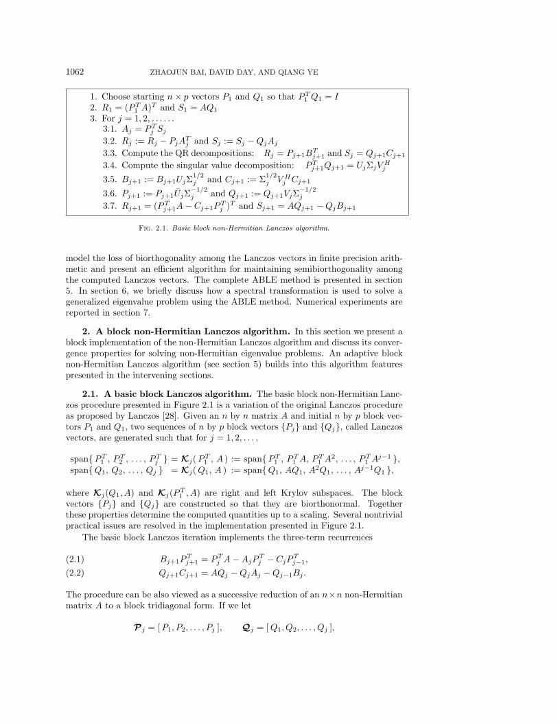
1. Choose starting n× p vectors P1 and Q1 so that PT1 Q1 = I2. R1 = (PT1 A)T and S1 = AQ1

3. For j = 1, 2, . . . . . .3.1. Aj = PTj Sj3.2. Rj := Rj − PjATj and Sj := Sj −QjAj3.3. Compute the QR decompositions: Rj = Pj+1B

Tj+1 and Sj = Qj+1Cj+1

3.4. Compute the singular value decomposition: PTj+1Qj+1 = UjΣjVHj

3.5. Bj+1 := Bj+1UjΣ1/2j and Cj+1 := Σ

1/2j V Hj Cj+1

3.6. Pj+1 := Pj+1UjΣ−1/2j and Qj+1 := Qj+1VjΣ

−1/2j

3.7. Rj+1 = (PTj+1A− Cj+1PTj )T and Sj+1 = AQj+1 −QjBj+1

Fig. 2.1. Basic block non-Hermitian Lanczos algorithm.

model the loss of biorthogonality among the Lanczos vectors in finite precision arith-metic and present an efficient algorithm for maintaining semibiorthogonality amongthe computed Lanczos vectors. The complete ABLE method is presented in section5. In section 6, we briefly discuss how a spectral transformation is used to solve ageneralized eigenvalue problem using the ABLE method. Numerical experiments arereported in section 7.

2. A block non-Hermitian Lanczos algorithm. In this section we present ablock implementation of the non-Hermitian Lanczos algorithm and discuss its conver-gence properties for solving non-Hermitian eigenvalue problems. An adaptive blocknon-Hermitian Lanczos algorithm (see section 5) builds into this algorithm featurespresented in the intervening sections.

2.1. A basic block Lanczos algorithm. The basic block non-Hermitian Lanc-zos procedure presented in Figure 2.1 is a variation of the original Lanczos procedureas proposed by Lanczos [28]. Given an n by n matrix A and initial n by p block vec-tors P1 and Q1, two sequences of n by p block vectors Pj and Qj, called Lanczosvectors, are generated such that for j = 1, 2, . . . ,

spanPT1 , PT2 , . . . , PTj = Kj(PT1 , A ) := spanPT1 , PT1 A, PT1 A2, . . . , PT1 Aj−1 ,

spanQ1, Q2, . . . , Qj = Kj(Q1, A ) := spanQ1, AQ1, A2Q1, . . . , A

j−1Q1 ,

where Kj(Q1, A) and Kj(PT1 , A) are right and left Krylov subspaces. The blockvectors Pj and Qj are constructed so that they are biorthonormal. Togetherthese properties determine the computed quantities up to a scaling. Several nontrivialpractical issues are resolved in the implementation presented in Figure 2.1.

The basic block Lanczos iteration implements the three-term recurrences

Bj+1PTj+1 = PTj A−AjPTj − CjPTj−1,(2.1)

Qj+1Cj+1 = AQj −QjAj −Qj−1Bj .(2.2)

The procedure can be also viewed as a successive reduction of an n×n non-Hermitianmatrix A to a block tridiagonal form. If we let

Pj = [P1, P2, . . . , Pj ], Qj = [Q1, Q2, . . . , Qj ],

ABLE METHOD 1063

and

Tj =

A1 B2

C2 A2. . .

. . .. . . BjCj Aj

,(2.3)

then the three-term recurrences (2.1) and (2.2) have the matrix form

PTj A = TjPTj + EjBj+1PTj+1,(2.4)

AQj =QjTj +Qj+1Cj+1ETj ,(2.5)

where Ej is a tall thin matrix whose bottom square is an identity matrix and whichvanishes otherwise. Furthermore, the computed Lanczos vectors Pj and Qj satisfythe biorthonormality

PTj Qj = I.(2.6)

When the blocksize p = 1, this is just the unblocked non-Hermitian Lanczos algorithmdiscussed in [20, p. 503].

Remark 1. For a complex matrix A we still use the transpose ·T instead of theconjugate transpose ·H . If A is complex symmetric and P1 = Q1, then (2.4) is thetranspose of (2.5), and it is necessary to compute only one of these two recurrencesprovided that a complex symmetric scaling scheme is used at step 3.4 in Figure 2.1.

Remark 2. The above block Lanczos algorithm can breakdown prematurely ifRTj Sj is singular (see step 3.6 in Figure 2.1). We will discuss this issue in section 3.

Remark 3. Many choices of the p×p nonsingular scaling matrices Bj+1 and Cj+1

satisfy RTj Sj = Bj+1Cj+1. The one presented here involves a little more work (com-

puting singular value decomposition (SVD) of PTj+1Qj+1), but it maintains that thelocal basis vectors in Pj+1 and Qj+1 are orthogonal and at the same time biorthogonalto each other. Furthermore, the singular values provide principal angles between thesubspaces spanned by Pj+1 and Qj+1, which is a measure of the quality of the basesconstructed (see Remark 4 below).

An alternative scaling maintains the unit length of all Lanczos vectors. Thisscaling scheme for the unblocked Lanczos algorithm is used in [17, 36, 14]. In this

case the Lanczos algorithm determines a pencil (Tj ,Ωj), where Tj is tridiagonal andΩj is diagonal. It can be shown that the tridiagonal Tj determined by the aboveunblocked (p = 1) Lanczos algorithm and this pencil are related by

Tj = ±|Ωj |1/2Tj |Ωj |1/2.

The Lanczos vectors are also related, up to sign, by a similar scaling.Remark 4. The condition numbers of the Lanczos vectors Pj and Qj can be

monitored by the diagonal matrices Σ1,Σ2, . . . ,Σj . Recall that the condition numberof the rectangular matrix Qj is defined by

cond(Qj) def= ‖Qj‖2‖Q†j‖2 =

‖Qj‖2σmin(Qj) ,


where σmin(Qj) = min‖x‖2=1 ‖Qjx‖2. To derive the bound for cond(Qj) observe from

step 3.6 in Figure 2.1 that ‖PTi ‖2 = ‖Qi‖2 = ‖Σ−1/2i ‖2. Then for a unit vector v such

that ‖PTj ‖2 = ‖PTj v‖2,

‖PTj ‖22 = ‖PTj v‖22 =

j∑i=1

‖PTi v‖22 ≤j∑i=1

1

min(Σi),

where min(Σi) denotes the smallest diagonal element of Σi. The latter bound alsoapplies toQj . Furthermore, we note that the biorthonormality condition (2.6) impliesthat ‖Pj‖2 σmin(Qj) ≥ 1. Therefore,

cond(Qj) ≤ ‖Pj‖2‖Qj‖2 ≤j∑i=1

1

min(Σi).

The bound applies to cond(Pj) by the similar argument. This generalizes and slightlyimproves a result from [36].

Remark 5. This implementation is a generalization of the block Hermitian Lanc-zos algorithms of Golub and Underwood [19] and Grimes, Lewis, and Simon [22] tothe non-Hermitian case. A simple version of the block non-Hermitian Lanczos proce-dure has been studied in [3]. Other implementations of the basic block non-HermitianLanczos procedure have been proposed for different applications in [7].

2.2. Eigenvalue approximation. To extract approximate the eigenvalues andeigenvectors of A, we solve the eigenvalue problem of the jp × jp block tridiagonalmatrix Tj after step 3.3 in Figure 2.1. Each eigentriplet (θ, wH , z) of Tj ,

wHTj = θwH and Tjz = zθ,

determines a Rayleigh–Ritz triplet , (θ, yH , x), where yH = wHPTj and x = Qjz.Rayleigh–Ritz triplets approximate eigentriplets of A.

To assess the approximation, (θ, yH , x), of an eigentriplet of the matrix A, let sand r denote the corresponding left and right residual vectors. Then by (2.4) and(2.5), we have

sH = yHA− θyH = (wHEj)Bj+1PTj+1,(2.7)

r = Ax− xθ = Qj+1Cj+1(ETj z).(2.8)

Note that a remarkable feature of the Lanczos algorithm is that the residual norms‖sH‖2 and ‖r‖2 are available without explicitly computing yH and x. There is noneed to form yH and x until their accuracy is satisfactory.

The residuals determine a backward error bound for the triplet. The biorthogo-nality condition, (2.6), applied to the definition of x and yH yields

PTj+1x = 0 and yHQj+1 = 0.(2.9)

From (2.8) and (2.7), we have the following measure of the backward error for theRayleigh–Ritz triplet (θ, yH , x):

yH(A− F ) = θyH and (A− F )x = xθ,

ABLE METHOD 1065

where the backward error matrix F is

F =rxH

‖x‖22+ysH

‖y‖22(2.10)

and ‖F‖2F = ‖r‖22/‖x‖22 + ‖sH‖22/‖y‖22. That is, the left and right residual normsbound the distance to the nearest matrix to A with eigentriplet (θ, yH , x). In fact ithas been shown that F is the smallest perturbation of A such that (θ, yH , x) is aneigentriplet of A − F [25]. The computed Rayleigh–Ritz value θ is a ‖F‖F -pseudoeigenvalue of the matrix A [51].

If we write A = B+F , where B = A−F , then a first-order perturbation analysisindicates that there is an eigenvalue λ of A such that

|λ− θ| ≤ cond(θ)‖F‖2,

where cond(θ) = ‖yH‖2 ‖x‖2/|yHx| is the condition number of the Rayleigh–Ritzvalue θ [20]. This first-order estimate is very often pessimistic because θ is a two-sided or generalized Rayleigh quotient [34]. A second-order perturbation analysisyields a more realistic error estimate, which should be used as a stopping criterion.Global second-order bounds for the accuracy of the generalized Rayleigh quotient maybe found in [49] and [9]. Here we derive an asymptotic bound.

Recall that (θ, yH , x) is an eigentriplet of B = A − F and that yHF = sH

and Fx = r. Assume that B has distinct eigenvalues θi and the correspondingnormalized left and right eigenvectors yHi , xi (‖yHi ‖2 = ‖xi‖2 = 1). Let us perturbθ = θ(0) toward an eigenvalue λ of A using the implicit function θ(t) = θ(B + tE)for E = F/‖F‖2. Under classical results from function theory [26], it can be shownthat in a neighborhood of the origin there exist differentiable θ(t), yH(t), and x(t)(‖yH(t)‖2 = ‖x(t)‖2 = 1) such that

yH(t)(B + tE) = θ(t)yH(t) and (B + tE)x(t) = x(t)θ(t).(2.11)

Next expand θ(t) about t = 0:

λ = θ(‖F‖2) = θ(0) + θ′(0)‖F‖2 +1

2θ′′(0)‖F‖22 +O(‖F‖32).

By differentiating (2.11) with respect to t, and setting t = 0, we obtain

θ′(0) =1

‖F‖2yHFx

yHx.

Note that from (2.10), yHFx = yHr + sHx. Substitute (2.7), (2.8), and (2.9) to findyHFx = 0. This implies the stationarity property θ′(0) = 0. Differentiate (2.11) withrespect to t twice, and set t = 0, and there appears

θ′′(0) =2

‖F‖2sH

yHxx′(0).

Now the standard eigenvector sensitivity analysis gives

x′(0) =∑θi 6=θ

yHi Ex

(θ − θi)yHi xixi.


See, for example, Golub and Van Loan [20, p. 345]. From the above two formulas, upto the second order of ‖F‖2, we obtain

|λ− θ| ≤ ‖sH‖2 ‖r‖2

gap(θ,B)

1

|yHx|∑θi 6=θ

1

|yHi xi|

.(2.12)

Here gap(θ,B) = minθi 6=θ |θ− θi|. Note that the term in the parentheses involves thecondition numbers of the eigenvalues θi of B.

The bound (2.12) shows that the accuracy of the Rayleigh–Ritz value θ is pro-portional to the product of the left and right residuals and the inverse of the gapin eigenvalues of B. We call this the semiquadratic convergence. Since gap(θ,B) isnot computable, we use the gap(θ, Tj) to approximate gap(θ,B) when ‖F‖2 is small.From (2.10) and (2.12), we advocate accepting θ as an approximate eigenvalue of A if

min

‖sH‖2, ‖r‖2, ‖s

H‖2 ‖r‖2gap(θ, Tj)

≤ τc,(2.13)

where τc is a given accuracy threshold. Note that for ill-posed problems, small resid-uals (backward errors) do not imply high eigenvalue accuracy (small forward error).In this case, the estimate is optimistic. In any case, since both the left and rightapproximate eigenvectors are available, the approximate eigenvalue condition num-bers are readily computable. This detects ill-posedness in an eigenvalue problem. Seenumerical example 5 in section 7.

It is well known that for Hermitian matrices, the Lanczos algorithm reveals firstthe outer and well-separated eigenvalues [35]. In the block Hermitian Lanczos algo-rithm with blocksize p, the outer eigenvalues and the eigenvalue clusters of order upto p that are well separated from the remaining spectra converge first [19, 41]. Thisqualitative understanding of convergence has been extended to the block Arnoldi al-gorithm for non-Hermitian eigenproblems in [42, 24].

2.3. Maintaining the biorthogonality of the Lanczos vectors. The quan-tities computed in the block Lanczos algorithm in the presence of finite precisionarithmetic have different properties than the corresponding exact quantities. Thebiorthogonality property, (2.6), fails to hold, and the columns of the matrices Pj andQj are spanning sets but not bases. The loss of linear independence in the matricesPj and Qj computed by the three-term recurrence is coherent; as a Rayleigh–Ritztriplet converges to an eigentriplet of A, copies of the Rayleigh–Ritz values appear.At this iteration, Qj is singular because it maps a group of right eigenvectors of Tjto an eigenvector of A.

For example, in a Lanczos run of 100 iterations, one may observe 5 copies ofthe dominant eigenvalue of A among the Rayleigh–Ritz values. This increases thenumber of iterations required to complete a given task. As a partial remedy, weadvocate maintaining local biorthogonality to ensure the biorthogonality among con-secutive Lanczos vectors in the three-term recurrences [14]. Local biorthogonality ismaintained as follows. After step 3.2 in Figure 2.1,

Rj := Rj − Pj(QTj Rj),Sj := Sj −Qj(PTj Sj).

Repeating this inner loop increases the number of floating point operations in a Lanc-zos iteration. However, no new data transfer is required, and without repetition

ABLE METHOD 1067

the local biorthogonality would normally be swamped. The cost effectiveness seemsindisputable.

Another limitation of simple implementations of the three-term recurrences isthat the multiplicity of an eigenvalue of A is not related in any practical way to themultiplicity of a Rayleigh–Ritz value. To reveal the multiplicity or clustering of aneigenvalue it typically suffices to explicitly enforce (2.6). This variation has beencalled a Lanczos algorithm with full rebiorthogonalization [38]. It is maintained byincorporating a variant of the Gram–Schmidt process called the two-sided modifiedGram–Schmidt biorthogonalization (TSMGS) [36]. After step 3.6 in Figure 2.1, webiorthogonalize Pj+1 and Qj+1 in place against all previous Lanczos vectors Pj =[P1, P2, . . . , Pj ] and Qj = [Q1, Q2, . . . , Qj ]:

for i = 1, 2, . . . , jPj+1 := Pj+1 − Pi(QTi Pj+1)Qj+1 := Qj+1 −Qi(PTi Qj+1)

endMaintaining full biorthogonality substantially increases the cost per iteration of theLanczos algorithm. To be precise, at Lanczos iteration j, an additional 8p2jn flopsis required. More importantly all the computed Lanczos vectors are accessed at eachiteration. This is very often the most costly part of a Lanczos run, although thereare cases where the matrix-vector multiplications may be the dominating factor. Aless-costly alternative to full biorthogonality is presented in section 4.

3. An adaptive block Lanczos algorithm. In this section, we present anadaptive block scheme. This algorithm has the flexibility to adjust the blocksize tothe multiplicity or the order of a cluster of desired eigenvalues. In addition, thealgorithm can be used to cure (near) breakdowns.

3.1. Augmenting the Lanczos vectors. In a variable block Lanczos algo-rithm, at the jth iteration, Pj and Qj have pj columns, respectively. At the next(j+ 1)th iteration, the number of columns of the Lanczos vectors Pj+1 and Qj+1 canbe increased by k as follows.

First note that for any n by k matrices Pj+1 and Qj+1, the basic three-term recur-

rences (2.1) and (2.2) also hold with augmented (j+1)th Lanczos vectors [Pj+1 Pj+1]

and [Qj+1 Qj+1]:

[Bj+1 0

] [ PTj+1

PTj+1

]= PTj A−AjPTj − CjPTj−1

and [Qj+1 Qj+1

] [ Cj+1

0

]= AQj −QjAj −Qj−1Bj .

Provided that [Pj+1 Pj+1

]T [Qj+1 Qj+1

](3.1)

is nonsingular , the Lanczos procedure continues as before under the substitutions

Pj+1 ←[Pj+1 Pj+1

], Qj+1 ←

[Qj+1 Qj+1

]


with proper normalization and

Bj+1 ←[Bj+1 0

], Cj+1 ←

[Cj+1

0

].

The only other constraint on Pj+1 and Qj+1 is that they satisfy the biorthogonalitycondition among the Lanczos vectors; i.e., it is required that

PTj+1Qj = 0 and PTj Qj+1 = 0.

As a consequence, the adaptive block scheme has the same governing equations andthe same resulting Rayleigh–Ritz approximation properties as the basic block Lanczosmethod described in section 2.

Before we turn to the usage of the adaptive block scheme, we discuss the choice ofthe increment vectors PTj+1 and Qj+1. Ideally we would like to choose augmentations

so that the resulting matrix PTj+1Qj+1 is well conditioned. To be precise we want

the smallest singular value of PTj+1Qj+1 to be larger than the given threshold τb, say

τb = 10−8 in double precision. However, there may not exist PTj+1 and Qj+1 such

that the given threshold τb is satisfied. A natural choice to choose Pj+1 and Qj+1 inpractice is to biorthogonalize a pair of random n by k vectors to the previous Lanczosvectors. In other words, the vectors Pj+1 and Qj+1 are computed by applying TSMGS(see section 2.3) to a pair of random n by k vectors. The construction is repeated afew times (say, 3 at most) if necessary to ensure that the smallest singular value of(3.1) is larger than a threshold. We observe that this works well in practice.

3.2. Adaptive blocking for clustered eigenvalues. If A has an eigenvalue ofmultiplicity greater than the blocksize, then the Rayleigh–Ritz values converge slowlyto this group of eigenvalues [12, 19, 22, 3]. In some applications, information aboutmultiplicity is available a priori and then the blocksize can be chosen accordingly. Butwhen this information is not available, it is desirable to adjust the blocksize using theinformation obtained during the iteration.

In any variable block implementation of the Lanczos algorithm in which thebiorthogonality of the computed Lanczos vectors is maintained, it is advantageousto increase the blocksize to the order of the largest cluster of Rayleigh–Ritz values,θi. The adaptive block scheme proposed in section 3.1 offers such flexibility.

The cluster of Rayleigh–Ritz values about θi is the set of all θk such that

|θi − θk| ≤ ηmax(|θi|, |θk|),(3.2)

where η is a user-specified clustering threshold. The order of the largest cluster ofRayleigh–Ritz values is computed whenever we test for convergence, and the blocksizeis increased to the order of the largest cluster.

3.3. Adapting the blocksize to treat breakdown. A second reason to in-crease the blocksize is to overcome a breakdown in the block Lanczos algorithm. Recallfrom section 2.1 that breakdown occurs when RTj Sj is singular. There are two cases:

I. Either Rj or Sj is rank deficient.II. Both Rj and Sj are not rank deficient but RTj Sj is.

Exact breakdowns are rare, but near breakdowns (i.e., RTj Sj has singular valuesclose to 0) do occur. In finite precision arithmetic this can cause numerical instability.

In case I, if Sj vanishes in step 3.2 of Figure 2.1 of the basic block Lanczosalgorithm, an invariant subspace is detected. To restart the Lanczos procedure choose

ABLE METHOD 1069

Qj+1 to be any vector such that PTj Qj+1 = 0. If Sj is just (nearly) rank deficient,then after the QR decomposition of Sj , Sj = Qj+1Cj+1, we biorthogonalize Qj+1

to the previous left Lanczos vectors Pj . This also effectively expands the Krylovsubspace and continues the procedure. Rank deficiency of Rj is treated similarly.Note that in this case, the blocksize is not changed. This generalizes the treatmentsuggested by Wilkinson for the unblocked Lanczos procedure [52, p. 389].

Case II is called a serious breakdown [52]. Let us first examine the case of exactbreakdown. Let Rj = Pj+1B

Tj+1 and Sj = Qj+1Cj+1 be the QR decompositions of

Rj and Sj . In this case, PTj+1Qj+1 is singular. Suppose that PTj+1Qj+1 has the SVD

PTj+1Qj+1 = U

[Σ 00 0

]V H ,

where Σ is nonsingular if it exists (Σ may be 0 by 0). Let us see how to augmentPj+1 and Qj+1 so that PTj+1Qj+1 is nonsingular. For clarity, drop the subscript j + 1

and partition PU and QV into

PU =[P(1) P(2)

]and QV =

[Q(1) Q(2)

].

Here the number of columns of P(2) and Q(2) is the number of zero singular values ofPTQ. Let the augmented Lanczos vectors be

P :=[P(1) P(2) P

]and Q :=

[Q(1) Q(2) Q

],

where

P = (I −Πj)T Q(2) and Q = (I −Πj)P(2).

Πj = QjPTj is the oblique projector. The biorthogonality condition (2.6) and then

the orthonormality of the columns of[P(1) P(2)

]yield

PT(1)Q = PT(1)(I −Πj)P(2) = PT(1)P(2) = 0

and

PT(2)Q = PT(2)(I −Πj)P(2) = PT(2)P(2) = I.

Similarly, PTQ(1) = 0 and PTQ(2) = I. Therefore, we have

PTQ =

Σ 0 00 0 I

0 I PT Q

,which is nonsingular for any PT Q. Therefore, we conclude that exact breakdowns arealways curable by the adaptive blocksize technique.

However, for the near breakdown case, the situation is more complicated. Theabove choice may not succeed in increasing the smallest singular value of PTj+1Qj+1

above a specific given threshold, τb. The difficulty involves the fact that the norms of Pand Q can be large because of the use of oblique projector Πj . In our implementation,

we have chosen P and Q by dualizing a pair of random n by k vectors to the previous


Lanczos vectors as described in section 3.1. The increment to the blocksize is thenumber of singular values of PTj+1Qj+1 below a specified threshold.

Another scheme for adjusting the block size to cure (near) breakdown is the look-ahead strategy [38, 17]. In the look-ahead Lanczos algorithm, the spans of the columnsof Pj and Qj remain within K(PT1 , A) and K(Q1, A), respectively. Specifically, PTj+1

and Qj+1 are augmented by

P = (I −Πj)TATPj+1 = ATPj+1 − PjCTj+1

and

Q = (I −Πj)AQj+1 = AQj+1 −QjBj+1.

If [Pj+1 PT ] [Qj+1 Q] is not (nearly) singular, then one step of look-ahead is successful

and Pj+1 and Qj+1 are obtained from P and Q, respectively, after normalization.Since

span(Qj+1) = span(Qj , [Qj+1, Q])

and

span(Qj+2) = span(Qj , [Qj+1, Q], A[Qj+1, Q])

= span(Qj+1, A2Qj+1),

Qj+2 has no more columns than Qj+1 prior to augmentation. That is, the blocksize doubles at step j + 1 only and then returns to the ambient block size at thefollowing step j+2. It may be necessary to repeatedly augment the (j+1)th Lanczosblock-vectors [36]. In contrast, we have shown that the adaptive strategy has theproperty that an exact breakdown is cured in using a fixed number of augmentationvectors. Moreover, to reveal clustered eigenvalues and to eliminate a potential sourceof slow convergence, we store Pj and Qj and maintain biorthogonality (see section4). We have found the adaptive block scheme to be a viable alternative to look-aheadstrategies here.

4. Maintaining semibiorthogonality. In this section we present a form oflimited rebiorthogonalization that is more efficient than the full rebiorthogonalizationdescribed in section 2.3. This method extends the block Hermitian Lanczos algorithmwith partial reorthogonalization to the non-Hermitian case [22]. Instead of maintain-ing full biorthogonality (section 2.3), only semibiorthogonality is maintained at eachiteration; i.e., for j ≥ 1,

dj+1 = max

(‖PTj Qj+1‖1‖Pj‖1‖Qj+1‖1 ,

‖QTj Pj+1‖1‖Qj‖1‖Pj+1‖1

)≤ √ε,(4.1)

where ε is the roundoff error unit. This generalizes the definition of semibiorthogonal-ity for the unblocked Lanczos algorithm [14]. We will show that semibiorthogonalityrequires less computation and data transfer to maintain than full biorthogonality. Inparticular, Pj and Qj are accessed only at certain iterations.

In section 4.1 we show how to monitor the loss of numerical biorthogonalitywithout significantly increasing the number of floating point operations in the Lanczosrecurrences. In section 4.2 we show how best to correct the loss of biorthogonality.

ABLE METHOD 1071

4.1. Monitoring the loss of biorthogonality. When the Lanczos algorithmis implemented in finite precision arithmetic, the computed quantities can be modeledby perturbed three-term recurrences:

Bj+1PTj+1 = PTj A−AjPTj − CjPTj−1 − FTj ,(4.2)

Qj+1Cj+1 = AQj −QjAj −Qj−1Bj −Gj ,(4.3)

where Fj and Gj represent the roundoff error introduced at iteration j. By applyingthe standard model of the rounding errors committed in floating point arithmetic [52],it can be shown that to first order in roundoff errors there holds

‖Fj‖F ≤ u(‖A‖1 ‖Pj‖1 + ‖Aj‖1 ‖Pj‖1 + ‖Cj‖1 ‖Pj−1‖1),

‖Gj‖F ≤ u(‖A‖1 ‖Qj‖1 + ‖Aj‖1 ‖Qj‖1 + ‖Bj‖1 ‖Qj−1‖1),

where u is a constant multiple of the roundoff error unit ε. The governing equationsfor the computed quantities are

PTj A = TjPTj + EjBj+1PTj+1 +FTj ,(4.4)

AQj =QjTj +Qj+1Cj+1ETj + Gj ,(4.5)

where the matrices F j = [F1, F2, . . . , Fj ] and Gj = [G1, G2, . . . , Gj ] are such that

max(‖F j‖F , ‖Gj‖F ) ≤ u(‖A‖1 + ‖Tj‖1) max(‖Pj‖F , ‖Qj‖F ).(4.6)

A detailed analysis for the unblocked case can be found in [2, 14].Now we use this model of rounding errors in the Lanczos process to quantify the

propagation of the loss of biorthogonality from iteration to iteration. The biorthogo-nality of the (j+1)th Lanczos vectors to the previous Lanczos vectors can be measuredusing the short vectors

Xj = PTj Qj+1 and Yj = PTj+1Qj .In the following, we show that these vectors satisfy perturbed three-term recurrenceswhich we can use to efficiently monitor the biorthogonality loss.

The recurrence for Xj is derived as follows. Note that

PTj Qj =

[Xj−1

0

]+ Ej .(4.7)

Let Wij = PTi Qj . Multiply (4.3) by PTj on the left, substitute in (4.4) × Qj , andthere appears

XjCj+1 = TjPTj Qj −PTj QjAj −PTj Qj−1Bj(4.8)

+ EjBj+1Wj+1,j +FTj Qj −PTj Gj .Substitute (4.7) above and (2.3), the definition of Tj , and simplify to find

TjPTj Qj −PTj QjAj = Tj

[Xj−1

0

]−[Xj−1

0

]Aj + Ej−1Bj .(4.9)

In addition, we have the identity

PTj Qj−1 =

Xj−2

00

+ Ej−1 +Wj,j−1Ej .(4.10)


Substituting (4.9) and (4.10) into (4.8) finally yields

XjCj+1 = Tj

[Xj−1

0

]−[Xj−1

0

]Aj −

Xj−2

0Wj,j−1

Bj(4.11)

+ EjBj+1Wj+1,j +O(uj),

where O(uj) represents the local rounding error term FTj Qj −PTj Gj and

uj = u(‖Tj‖1 + ‖A‖1) max(‖Pj‖F , ‖Qj‖F ).

The similar analysis of the left Lanczos vectors yields

Bj+1Yj = [Yj−1, 0 ]Tj −Aj [Yj−1, 0 ]− Cj [Yj−2, 0, Wj−1,j ](4.12)

+ Wj,j+1Cj+1Ej +O(uj).

Equations (4.11) and (4.12) model the propagation of the loss of the numericalbiorthogonality among Lanczos vectors from iteration to iteration. The followingalgorithm implements these recurrence relations to monitor the biorthogonality loss.Note that the scalar parameter dj+1 is our measure of the biorthogonality. When

dj+1 >√ε, then TSMGS is invoked to recover biorthogonality as described in the

next section.1

Algorithm for monitoring the loss of biorthogonality.Initially, when j = 1, we set X1 = 0, Y1 = 0, d1 = u, compute

X2 = PT1 Q2, Y2 = PT2 Q1, and let W(l)1 = Y2, W

(r)1 = X2. When

j > 1.

1. W(l)2 = PTj+1Qj

2. X3 = Tj

[X2

0

]−[X2

0

]Aj −

[X1

W(l)1

]Bj +

[0

Bj+1W(l)2

]3. X3 := (X3 + Fj)C

−1j+1

4. X1 =

[X2

0

]; X2 = X3

5. W(r)2 = PTj Qj+1

6. Y3 =[Y2 0

]Tj−Aj

[Y2 0

]−Cj [ Y1 W(r)1

]+[

0 W(r)2 Cj+1

]7. Y3 := B−1

j+1(Y3 + FTj )

8. Y1 =[Y2 0

]; Y2 = Y3

9. W(l)1 = W

(l)2 ; W

(r)1 = W

(r)2

10. dj+1 = max(‖X2‖1/(‖Pj‖1‖Qj+1‖1), ‖Y2‖∞/(‖Qj‖1‖Pj+1‖1))The matrix Fj is a random matrix scaled to have norm uj to simulate the roundofferrors in the three-term recurrences. The number of floating point operations periteration of the monitoring algorithm is 2j2 +O(n), where the 2j2 is for the multipli-cations by Tj in steps 2 and 6 above and the n comes from the “inner products” ofblock Lanczos vectors in steps 1 and 5 above. If the block tridiagonal structure of Tjis taken in account, then the cost is just O(n). Therefore the cost of the monitoringalgorithm is not significant, as promised.

1To economize on storage there is a subtle change of notation in the following monitoring algo-rithm. At Lanczos iteration j, the vectors Xj−1, Xj , and Xj+1 are denoted X1, X2, and X3, andthe previous Xk are not stored. Similar conventions apply to Yi and Wi,k.

ABLE METHOD 1073

4.2. Correcting the loss of biorthogonality. When action is required tomaintain semibiorthogonality (4.1), TSMGS (see section 2.3) is invoked to rebiortho-normalize or correct the candidate Lanczos vectors Pj+1 and Qj+1. Recall from (4.11)that the sequence Xj satisfies a perturbed three-term recurrence. Correcting Qj+1

annihilates the O(√ε) matrix Xj , but at the next Lanczos iteration Xj+1 will be a

multiple of the nearly O(√ε) matrix Xj−1. Instead, as Qj+1 is corrected to maintain

semibiorthogonality, we also correct Qj ; in this way the biorthogonality of the fol-lowing Lanczos vectors can deteriorate gradually. The similar comments hold for theleft Lanczos vectors. There is a much better way to do this than to apply TSMGSat consecutive iterations to the pairs of Pj and Qj and Pj+1 and Qj+1, respectively.Instead, as the columns of Pj and Qj are transferred from slow storage to the com-putational unit to correct Pj+1 and Qj+1, the previous Lanczos vectors Pj and Qjalso can be retroactively corrected. This halves the amount of data transfer required.

Retroactive TSMGS. Biorthogonalize Pj , Pj+1, Qj , and Qj+1 against theprevious Lanczos vectors in place.

for i = 1, 2, . . . , j − 1

Pj := Pj − Pi(QTi Pj)Pj+1 := Pj+1 − Pi(QTi Pj+1)

Qj := Qj −Qi(PTi Qj)Qj+1 := Qj+1 −Qi(PTi Qj+1)

end

Pj+1 := Pj+1 − Pj (QTj Pj+1)

Qj+1 := Qj+1 −Qj(PTj Qj+1)

We do not update the QR decompositions and SVDs computed in the basic Lanczosalgorithm after retroactive TSMGS for the same technical reasons discussed in section6.3 of [14] for the unblocked Lanczos algorithm.

5. The ABLE method. In summary, the ABLE method presented in Figure5.1 incorporates an adaptive blocking scheme (section 3) into the basic block Lanczosalgorithm (section 2) and maintains the local and semibiorthogonality of Lanczosvectors (section 4). Specifically, we have the following:

• At step 3.3, we suggest the use of (2.13) in section 2.2 as the stopping criterion.Then, at the end of a Lanczos run, we compute the residual norms ‖sH‖2 and‖r‖2 corresponding to the converged Rayleigh–Ritz triplets (θ, yH , x). See(2.7) and (2.8) in section 2.2. Note that the theory in section 2.2 is basedon the exact biorthogonality. When only semibiorthogonality is maintained,θ′(0) is no longer zero. However, using (4.4), (4.5), and semibiorthogonality(4.1), it is easy to see that θ′(0) is still in the magnitude of

√ε. Thus, as far as

‖F‖2 is not too small (not less than O(√ε)), the second term in the expansion

for λ still dominates the first term θ′(0)‖F‖2, and therefore, (2.13) would bevalid. (Specifically, yHr ∼ √ε‖r‖2 and the first term in the expansion satisfiesθ′(0)‖F‖2 ∼ 1

|yHx|√ε‖F‖2.)

• At step 3.4, (3.2) is used to compute the order of the largest cluster as de-scribed in section 3.2.• For step 3.7, see section 3.3 for an explanation.• At step 3.9, τb is a threshold for breakdown. min(Σ) is the smallest singular

value of the matrix PTj+1Qj+1. If there is (near) breakdown and/or the orderof the largest cluster of the converged Rayleigh–Ritz values is larger than theblocksize, then the blocks are augmented as described in section 3.1.


1. Choose starting vectors P1 and Q1 so that PT1 Q1 = I2. R = (PT1 A)T and S = AQ1

3. For j = 1, 2, . . . until convergence3.1. Aj = PTj S

3.2. R := R− PjATj and S := S −QjAj3.3. Compute the eigen-decomposition of Tj , and test for convergence3.4. Find the largest order δ of the clustering of converged Rayleigh–Ritz

values3.5. Local biorthogonality: R := R− Pj(QTj R) and S := S −Qj(PTj S)

3.6. Compute the QR decompositions: R = Pj+1BTj+1 and S = Qj+1Cj+1

3.7. If R or S (or both) is rank deficient, apply TSMGS to biorthogonalizePj+1 and Qj+1 against the previous Lanczos vectors

3.8. Compute the SVD: PTj+1Qj+1 = UΣV H

3.9. Increase blocksize if min(Σ) < τb and/or δ > pj3.10. Bj+1 := Bj+1UΣ1/2 and Cj+1 := Σ1/2V HCj+1

3.11. Pj+1 := Pj+1UΣ−1/2 and Qj+1 := Qj+1V Σ−1/2

3.12. Monitor the loss of biorthogonality, and correct if necessary3.13. R = (PTj+1A− Cj+1P

Tj )T and S = AQj+1 −QjBj+1

Fig. 5.1. ABLE method.

• Algorithms for monitoring the loss of biorthogonality and maintaining semibi-orthogonality at step 3.12 are described in sections 4.1 and 4.2.

The non-Hermitian Lanczos algorithm is also called the two-sided Lanczos algo-rithm because both the operations

XTA and AX

are required at each iteration. A is referenced only as a rule to compute these matrix-vector products. Because of this feature, the algorithm is well suited for large sparsematrices or large structured dense matrices for which matrix-vector products can becomputed cheaply. The efficient implementation of these products depends on thedata structure and storage format for the A matrix and the Lanczos vectors.

If no Lanczos vectors are saved, the three-term recurrences can be implementedusing only six block vectors of length n. To maintain the semibiorthogonality of thecomputed Lanczos vectors Pj and Qj , it is necessary to store these vectors in coreor out-of-core memory. This consumes a significant amount of memory. The usermust be conscious of how much memory is needed for each application. For verylarge matrices it may be best to store the Lanczos vectors out-of-core. After eachLanczos iteration, save the current Lanczos vectors to an auxiliary storage device.The Lanczos vectors are recalled in the procedure TSMGS for rebiorthogonalizationand when the converged Rayleigh–Ritz vectors are computed at the end of a Lanczosrun.

A block Lanczos algorithm is ideal for application codes that represent A out-of-core. The main cost of a Lanczos iteration, with or without blocks, is accessing A.Block algorithms compute the matrix block vectors product with only one pass overthe data structure defining A, with a corresponding savings of work.

The most time-consuming steps in a Lanczos run are to1. apply the matrix A (from the left and the right),2. apply retroactive TSMGS to maintain semibiorthogonality, and

ABLE METHOD 1075

3. solve the eigenproblem for the block tridiagonal matrix Tj when j increases.Items 1 and 2 have been addressed already (see the above and section 4.2). For item3, we presently use the QR algorithm for Tj . We note that it is not necessary to solvethe eigenproblem for Tj at each Lanczos iteration. A way to reduce such cost is tosolve the eigenvalue problem for Tj only after a correction iteration has been madeto maintain semibiorthogonality. This technique utilizes the connection between theloss of the biorthogonality and convergence [33, 35, 2].

6. A spectral transformation ABLE method. In this section we brieflydiscuss how to use the ABLE method to compute some eigenvalues of the generalizedeigenvalue problem

Kx = λMx(6.1)

nearest an arbitrary complex number, σ. We assume that K−σM is nonsingular andthat it is feasible to solve the linear system of equations with coefficient matrix K −σM . The reward for solving this linear system of equations is the rapid convergence ofthe Lanczos algorithm. In section 7 we apply the ABLE method to such a generalizedeigenvalue problem arising in magneto-hydro-dynamics (MHD).

We apply a popular shift-and-invert strategy to the pair (K,M) with shift σ [16].In this approach, the ABLE method is applied with

A = (K − σM)−1M.(6.2)

The eigenvalues, µ, of A are µ = 1/(λ − σ). The outer eigenvalues of A are nowthe eigenvalues of (K,M) nearest to σ. This spectral transformation also generallyimproves the separation of the eigenvalues of interest from the remaining eigenvaluesof (K,M), a very desirable property.

When we apply the ABLE method to the matrix A = (K − σM)−1M , the gov-erning equations become

PTj (K − σM)−1M = TjPTj + EjBj+1PTj+1,(6.3)

(K − σM)−1MQj =QjTj +Qj+1Cj+1ETj .(6.4)

If (θ, wH , z) is an eigentriplet of Tj , then from the above governing equations (6.3)and (6.4), the triplet(

λ, yH , x)

:=

(σ +

1

θ, wHPTj (K − σM)−1, Qjz

)is an approximate eigentriplet of the matrix pair (K,M). The corresponding left andright residuals are

sH = yHK − λyHM = −1

θwHEjBj+1P

Tj+1,

r = Kx− λMx = −1

θ(K − σM)Qj+1Cj+1E

Tj z.

The matrix-vector products Y = [(K−σM)−1M ]X and ZT = XT [(K−σM)−1M ]required in the inner loop of the algorithm can be performed by first computing theLU factorization of K − σM = LU and then solving the linear systems of equationsLUY = MX and ZT = XT (LU)−1M for Y and ZT , respectively.


If K and M are real, and the shift σ is complex, one can still keep the Lanczosprocedure in real arithmetic using a strategy proposed by Parlett and Saad [37].

In many applications, M is symmetric positive definite. In this case, one can avoidfactoring M explicitly by preserving M -biorthogonality among the Lanczos vectors[16, 35, 11, 22]. Numerical methods for the case in which M is symmetric indefiniteare discussed in [22, 32].

7. Summary of numerical examples. This section summarizes our numericalexperience with the ABLE method. We have selected test eigenvalue problems fromreal applications to demonstrate the major features of the ABLE method. Eachnumerical example illustrates a property of the ABLE method. All test matricespresented here can be found in the test matrix collection for non-Hermitian eigenvalueproblems [4].

The ABLE method has been implemented in Matlab 4.2 with sparse matrix com-putation functions. All numerical experiments are performed on a SUN Sparc 10workstation with IEEE double precision floating point arithmetic. The tolerancevalue τc for the stopping criterion (2.13) is set to be 10−8. The clustering threshold(3.2) is η = 10−6. The breakdown threshold is τb = 10−8.

Example 1. The block algorithm accelerates convergence in the presence of mul-tiple and clustered eigenvalues. When the desired eigenvalues are known in advanceto be multiple or clustered, we should initially choose the blocksize as the expectedmultiplicity or the cluster order. For example, the largest eigenvalue of the 656× 656Chuck matrix has multiplicity 2. If we use the unblocked ABLE method, then atiteration 20 the converged Rayleigh–Ritz values,

5.502378378875370e+ 00,1.593971696766128e+ 00,

approximate the two largest distinct eigenvalues. But the multiplicity is not yetrevealed. However, if we use the ABLE method with initial blocksize 2, then atiteration 7 the converged Rayleigh–Ritz values are

5.502378378347202e+ 00,5.502378378869873e+ 00.

Each computed Rayleigh–Ritz value agrees to 10 to 12 decimal digits compared withthe one computed by the dense QR algorithm.

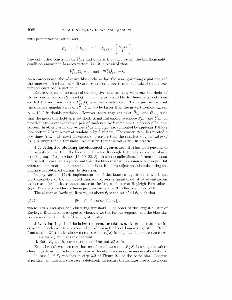
Example 2. Full biorthogonality is very expensive to maintain in terms of floatingpoint operations and memory access. Based on our experience, maintaining semibi-orthogonality is a reliable and much less expensive alternative. Our example is a2500 × 2500 block tridiagonal coefficient matrix obtained by discretizing the two-dimensional model convection-diffusion differential equation

−∆u+ 2p1ux + 2p2uy − p3u = f in Ω,

u = 0 on ∂Ω

using finite differences, where Ω is the unit square (x, y) ∈ R2, 0 ≤ x, y ≤ 1.The eigenvalues of the coefficient matrix can be expressed analytically in terms ofthe parameters p1, p2, and p3. In our test run, we choose p1 = 0.5, p2 = 2, andp3 = 1. For this set of parameters, all eigenvalues of the resulting matrix A arepositive real and distinct. With full biorthogonality, at iteration 132, the two largest

ABLE METHOD 1077

20 40 60 80 100 120

10-14

10-12

10-10

10-8

10-6

10-4

10-2

100

Lanczos step

bior

thog

onal

ity

Estimated (dash dot) and Exact (solid) Duality, Omega (+)

Fig. 7.1. The exact (solid line) and estimated (dash-dot line) biorthogonality of the Lanczosvectors and the smallest singular values (+) of PTj+1Qj+1.

eigenvalues are converged. If we use the ABLE method with semibiorthogonality, atiteration 139, the same two largest eigenvalues are converged to the same accuracy.The difference is that only 8 corrections of biorthogonality loss are invoked to maintainsemibiorthogonality, compared to 132 corrections for full biorthogonality.

In Figure 7.1 the solid and dotted lines display the exact and estimated biorthog-onality of the computed Lanczos vectors, and the “+”-points concern breakdown andare the smallest singular values of PTj Qj . The solid line plots

dj+1 = max

(‖PTj Qj+1‖1‖Pj‖1‖Qj+1‖1 ,

‖QTj Pj+1‖1‖Qj‖1‖Pj+1‖1

)for j = 1, 2, . . . , 132. Each sharp decrease corresponds to a correction. The dottedline plots the estimate, dj+1, of this quantity computed by the monitoring algorithmof section 4.2. Correction iterations are taken when the dotted line increases to thethreshold

√ε, where ε denotes the machine precision. The observation that the solid

line is below the dotted line indicates that the monitoring algorithm is prudent. Anear breakdown occurs if the smallest singular value of PTj+1Qj+1 is less than thebreakdown threshold, but this is not the case in this example.

Example 3. As mentioned before, when we know the multiplicity of the eigenvaluesin advance, we should choose the appropriate blocksize, otherwise the adaptive schemepresented in section 3 can dynamically adjust the blocksize to accelerate convergence.This smooths the convergence behavior to clusters of eigenvalues. For example, weapply the ABLE method with initial blocksize 1 to the 656 × 656 Chuck matrix. Atiteration 24, the double eigenvalue is detected and the blocksize is doubled.

Example 4. Exact breakdowns are rare but near breakdowns are not. In general,we can successfully cure the near breakdowns. For example, when the ABLE methodis applied to the 882 × 882 Quebec Hydro matrix from the application of numerical


0 5 10 15 20 25 30−8

−6

−4

−2

0

2

4

6

8

real part

imag

inar

y pa

rt

Eigenvalues (+) and Rayleigh−Ritz values (o)

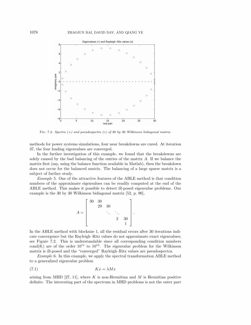
Fig. 7.2. Spectra (+) and pseudospectra () of 30 by 30 Wilkinson bidiagonal matrix.

methods for power systems simulations, four near breakdowns are cured. At iteration37, the four leading eigenvalues are converged.

In the further investigation of this example, we found that the breakdowns aresolely caused by the bad balancing of the entries of the matrix A. If we balance thematrix first (say, using the balance function available in Matlab), then the breakdowndoes not occur for the balanced matrix. The balancing of a large sparse matrix is asubject of further study.

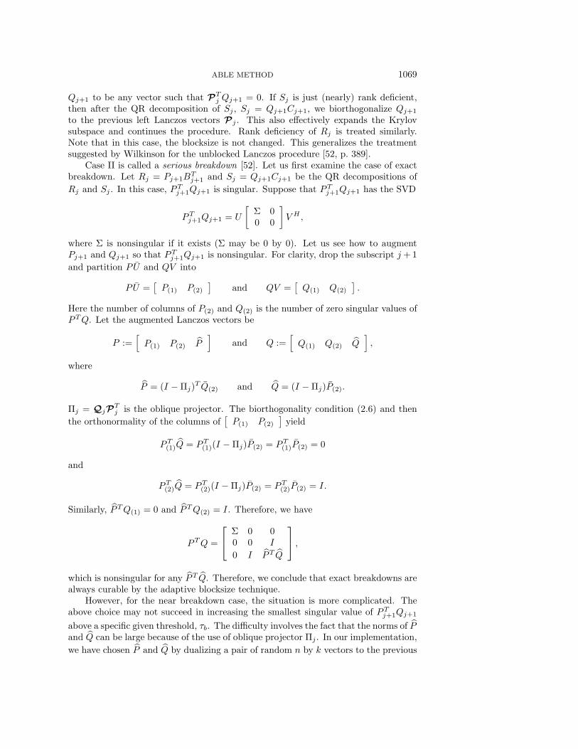
Example 5. One of the attractive features of the ABLE method is that conditionnumbers of the approximate eigenvalues can be readily computed at the end of theABLE method. This makes it possible to detect ill-posed eigenvalue problems. Ourexample is the 30 by 30 Wilkinson bidiagonal matrix [52, p. 90],

A =

30 30

29 30. . .

. . .

2 301

.In the ABLE method with blocksize 1, all the residual errors after 30 iterations indi-cate convergence but the Rayleigh–Ritz values do not approximate exact eigenvalues;see Figure 7.2. This is understandable since all corresponding condition numberscond(θi) are of the order 1011 to 1013. The eigenvalue problem for the Wilkinsonmatrix is ill-posed and the “converged” Rayleigh–Ritz values are pseudospectra.

Example 6. In this example, we apply the spectral transformation ABLE methodto a generalized eigenvalue problem

Kx = λMx(7.1)

arising from MHD [27, 11], where K is non-Hermitian and M is Hermitian positivedefinite. The interesting part of the spectrum in MHD problems is not the outer part

ABLE METHOD 1079

of the spectrum but an internal branch, known as the Alfven spectrum. We need touse a spectral transformation technique to transfer the interesting spectrum to theouter part. In section 6, we have outlined a general approach. Now, we show thenumerical results of this general approach for the MHD test problem. Both K andM are 416 by 416 block tridiagonal matrices with 16 by 16 blocks. To two significantdigits, there holds

‖K‖1 = 3100 and ‖M‖1 = 2.50,

but the estimated condition number of M is 5.05×109; M is quite ill conditioned. Thecomputational task is to calculate the eigenvalues close to the shift σ = −0.3 + 0.65i[8].

We ran the unblocked spectral transformation ABLE method. After only 30iterations, 10 Rayleigh–Ritz values are converged; their accuracy ranges from 10−8 to10−12, compared with the eigenvalues computed by the QZ algorithm. The followingtable lists the 10 converged Rayleigh–Ritz values θi and the corresponding left andright residual norms, where

Res-Li =‖yHi K − θiyHi M‖2max(‖K‖1, ‖M‖1)

, Res-Ri =‖Kxi − θiMxi‖2

max(‖K‖1, ‖M‖1),

and (yHi , xi) are the normalized approximate left and right eigenvectors of (K,M)(i.e., ‖yHi ‖2 = ‖xi‖2 = 1):

i θi Res-Li Res-Ri

1 −2.940037576164888e− 01 + 5.871546479737660e− 01i 3.82e− 12 6.59e− 112 −2.381814888866186e− 01 + 5.914958688660595e− 01i 2.66e− 11 4.46e− 113 −3.465530921874517e− 01 + 5.468970786348115e− 01i 1.23e− 11 2.76e− 104 −3.780991425908282e− 01 + 5.071655448857557e− 01i 6.18e− 11 3.98e− 105 −2.410301845692590e− 01 + 5.238090347100917e− 01i 9.81e− 11 4.32e− 106 −1.989292783177918e− 01 + 5.900118523050361e− 01i 5.34e− 11 8.55e− 117 −2.045328538082208e− 01 + 5.678048139549289e− 01i 5.97e− 11 1.12e− 108 −3.092857309948118e− 01 + 4.687528684165645e− 01i 5.23e− 09 2.59e− 089 −1.749780170739634e− 01 + 5.920044440850396e− 01i 5.62e− 10 9.58e− 1010 −1.573456542107287e− 01 + 5.976613227972810e− 01i 5.98e− 09 9.63e− 09

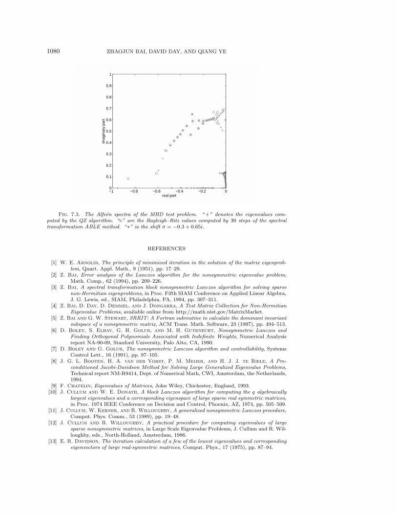
In addition, six other Rayleigh–Ritz values range in accuracy from 10−5 to 10−7.Figure 7.3 shows Alfven spectrum computed by the QZ algorithm (+) and the Ray-leigh–Ritz values () computed by the spectral transformation ABLE method.

Three corrections to maintain semibiorthogonality were taken at iterations 13,20, and 26. The convergence history of the Rayleigh–Ritz values are shown in thefollowing table, where j is the Lanczos iteration and k is the number of convergedRayleigh–Ritz values at the jth iteration:

j ≤ 14 15–18 19 20–22 23–24 25–26 27–28 29 30k 0 1 2 3 4 7 8 9 10

Moreover, at Lanczos iteration 45, the entire Alfven branch of spectra of the MHD testproblem are revealed: 20 Rayleigh–Ritz values converged, and 12 other Rayleigh–Ritzvalues range in accuracy from 10−7 up to 10−5. No copies of eigenvalues are observed.

Acknowledgments. The authors would like to thank the referees for their valu-able comments on the manuscript.


−1 −0.8 −0.6 −0.4 −0.2 00

0.1

0.2

0.3

0.4

0.5

0.6

0.7

0.8

0.9

1

real part

imag

inar

y pa

rt

Fig. 7.3. The Alfven spectra of the MHD test problem. “ +” denotes the eigenvalues com-puted by the QZ algorithm. “” are the Rayleigh–Ritz values computed by 30 steps of the spectraltransformation ABLE method. “ ∗” is the shift σ = −0.3 + 0.65i.

REFERENCES

[1] W. E. Arnoldi, The principle of minimized iteration in the solution of the matrix eigenprob-lem, Quart. Appl. Math., 9 (1951), pp. 17–29.

[2] Z. Bai, Error analysis of the Lanczos algorithm for the nonsymmetric eigenvalue problem,Math. Comp., 62 (1994), pp. 209–226.

[3] Z. Bai, A spectral transformation block nonsymmetric Lanczos algorithm for solving sparsenon-Hermitian eigenproblems, in Proc. Fifth SIAM Conference on Applied Linear Algebra,J. G. Lewis, ed., SIAM, Philadelphia, PA, 1994, pp. 307–311.

[4] Z. Bai, D. Day, D. Demmel, and J. Dongarra, A Test Matrix Collection for Non-HermitianEigenvalue Problems, available online from http://math.nist.gov/MatrixMarket.

[5] Z. Bai and G. W. Stewart, SRRIT: A Fortran subroutine to calculate the dominant invariantsubspace of a nonsymmetric matrix, ACM Trans. Math. Software, 23 (1997), pp. 494–513.

[6] D. Boley, S. Elhay, G. H. Golub, and M. H. Gutknecht, Nonsymmetric Lanczos andFinding Orthogonal Polynomials Associated with Indefinite Weights, Numerical Analysisreport NA-90-09, Stanford University, Palo Alto, CA, 1990.

[7] D. Boley and G. Golub, The nonsymmetric Lanczos algorithm and controllability, SystemsControl Lett., 16 (1991), pp. 97–105.

[8] J. G. L. Booten, H. A. van der Vorst, P. M. Meijer, and H. J. J. te Riele, A Pre-conditioned Jacobi-Davidson Method for Solving Large Generalized Eigenvalue Problems,Technical report NM-R9414, Dept. of Numerical Math, CWI, Amsterdam, the Netherlands,1994.

[9] F. Chatelin, Eigenvalues of Matrices, John Wiley, Chichester, England, 1993.[10] J. Cullum and W. E. Donath, A block Lanczos algorithm for computing the q algebraically

largest eigenvalues and a corresponding eigenspace of large sparse real symmetric matrices,in Proc. 1974 IEEE Conference on Decision and Control, Phoenix, AZ, 1974, pp. 505–509.

[11] J. Cullum, W. Kerner, and R. Willoughby, A generalized nonsymmetric Lanczos procedure,Comput. Phys. Comm., 53 (1989), pp. 19–48.

[12] J. Cullum and R. Willoughby, A practical procedure for computing eigenvalues of largesparse nonsymmetric matrices, in Large Scale Eigenvalue Problems, J. Cullum and R. Wil-loughby, eds., North-Holland, Amsterdam, 1986.

[13] E. R. Davidson, The iteration calculation of a few of the lowest eigenvalues and correspondingeigenvectors of large real-symmetric matrices, Comput. Phys., 17 (1975), pp. 87–94.

ABLE METHOD 1081

[14] D. Day, Semi-Duality in the Two-Sided Lanczos Algorithm, Ph.D. thesis, University of Cali-fornia, Berkeley, CA, 1993.

[15] I. Duff and J. Scott, Computing selected eigenvalues of sparse nonsymmetric matrices usingsubspace iteration, ACM Trans. Math. Software, 19 (1993), pp. 137–159.

[16] T. Ericsson and A. Ruhe, The spectral transformation Lanczos method for the numericalsolution of large sparse generalized symmetric eigenvalue problem, Math. Comp., 35 (1980),pp. 1251–1268.

[17] R. W. Freund, M. H. Gutknecht, and N. M. Nachtigal, An implementation of the look-ahead Lanczos algorithm for non-Hermitian matrices, SIAM J. Sci. Comput., 14 (1993),pp. 137–158.

[18] R. W. Freund, N. M. Nachtigal, and J. C. Reeb, QMRPACK User’s Guide, Technicalreport ORNL/TM-12807, Oak Ridge National Laboratory, Oak Ridge, TN, 1994.

[19] G. Golub and R. Underwood, The block Lanczos method for computing eigenvalues, inMathematical Software III, J. Rice, ed., Academic Press, New York, 1977, pp. 364–377.

[20] G. Golub and C. Van Loan, Matrix Computations, 2nd ed., Johns Hopkins University Press,Baltimore, MD, 1989.

[21] W. B. Gragg, Matrix interpretations and applications of the continued fraction algorithm,Rocky Mountain J. Math., 5 (1974), pp. 213–225.

[22] R. Grimes, J. Lewis, and H. Simon, A shifted block Lanczos algorithm for solving sparsesymmetric generalized eigenproblems, SIAM J. Matrix Anal. Appl., 15 (1994), pp. 228–272.

[23] M. H. Gutknecht, A completed theory of the unsymmetric Lanczos process and related algo-rithms, Parts I and II, SIAM J. Matrix Anal. Appl., Part I, 13 (1992), pp. 594–639, PartII, 15 (1994), pp. 15–58.

[24] Z. Jia, Generalized block Lanczos methods for large unsymmetric eigenproblems, Numer. Math.,80 (1998), pp. 239–266.

[25] W. Kahan, B. N. Parlett, and E. Jiang, Residual bounds on approximate eigensystems ofnonnormal matrices, SIAM J. Numer. Anal., 19 (1982), pp. 470–484.

[26] T. Kato, Perturbation Theory for Linear Operators, 2nd ed., Springer-Verlag, Berlin, 1980.[27] W. Kerner, Large-scale complex eigenvalue problems, J. Comput. Phys., 85 (1989), pp. 1–85.[28] C. Lanczos, An iteration method for the solution of the eigenvalue problem of linear differential

and integral operators, J. Res. Natl. Bur. Stand, 45 (1950), pp. 225–280.[29] R. Lehoucq, Analysis and Implementation of an Implicitly Restarted Arnoldi Iterations, Ph.D.

thesis, Rice University, Houston, Texas, 1995.[30] R. Lehoucq and J. A. Scott, An Evaluation of Software for Computing Eigenvalues of

Sparse Nonsymmetric Matrices, Preprint MCS-P547-1195, Argonne National Laboratory,Argonne, IL, 1996.

[31] R. Lehoucq, D. Sorensen, and C. Yang, ARPACK Users’ Guide: Solution of Large ScaleEigenvalue Problems by Implicitly Restarted Arnoldi Methods, SIAM, Phildelphia, PA,1998.

[32] K. Meerbergen and A. Spence, Implicitly Restarted Arnoldi with Purification for the Shift-Invert Transformation, report tw 225, Dept. of Comput. Sci., Katholieke Universiteit Leu-ven, Belgium, 1995.

[33] C. Paige, The Computation of Eigenvalues and Eigenvectors of Very Large Sparse Matrices,Ph.D. thesis, London University, London, UK, 1971.

[34] B. Parlett, The Rayleigh quotient algorithm iteration and some generalizations for nonnor-mal matrices, Math. Comp., 28 (1974), pp. 679–693.

[35] B. Parlett, The Symmetric Eigenvalue Problem, Prentice-Hall, Englewood Cliffs, NJ, 1980.[36] B. Parlett, Reduction to tridiagonal form and minimal realizations, SIAM J. Matrix Anal.

Appl., 13 (1992), pp. 567–593.[37] B. Parlett and Y. Saad, Complex shift and invert strategies for real matrices, Linear Algebra

Appl., 88/89 (1987), pp. 575–595.[38] B. N. Parlett, D. R. Taylor, and Z. A. Liu, A look-ahead Lanczos algorithm for unsym-

metric matrices, Math. Comp., 44 (1985), pp. 105–124.[39] A. Ruhe, Implementation aspects of band Lanczos algorithms for computation of eigenvalues

of large sparse symmetric matrices, Math. Comp., 33 (1979), pp. 680–687.[40] A. Ruhe, Rational Krylov, a Practical Algorithm for Large Sparse Nonsymmetric Matrix Pen-

cils, Computer Science Division UCB/CSD-95-871, University of California, Berkeley, CA,1995.

[41] Y. Saad, On the rates of convergence of the Lanczos and block Lanczos methods, SIAM J.Numer. Anal., 17 (1980), pp. 687–706.

[42] Y. Saad, Variations on Arnoldi’s method for computing eigenelements of large unsymmetric


matrices, Linear Algebra Appl., 34 (1980), pp. 269–295.[43] Y. Saad, Numerical Methods for Large Eigenvalue Problems, Halsted Press (division of John

Wiley), New York, 1992.[44] M. Sadkane, Block-Arnoldi and Davidson methods for unsymmetric large eigenvalue problems,

Numer. Math., 64 (1993), pp. 195–211.[45] M. Sadkane, A block Arnoldi-Chebyshev method for computing the leading eigenpairs of large

sparse unsymmetric matrices, Numer. Math., 64 (1993), pp. 181–193.[46] H. Simon, The Lanczos algorithm with partial reorthogonalization, Math. Comp., 42 (1984),

pp. 115–142.[47] G. L. G. Sleijpen and H. A. van der Vorst, A Jacobi-Davidson iteration method for linear

eigenvalue problems, SIAM J. Matrix Anal. Appl., 17 (1996), pp. 401–425.[48] D. Sorensen, Implicit application of polynomial filters in a k-step Arnoldi method, SIAM J.

Matrix Anal. Appl., 13 (1992), pp. 357–385.[49] G. W. Stewart, Error and perturbation bounds for subspaces associated with certain eigen-

value problems, SIAM Rev., 15 (1973), pp. 727–764.[50] W. J. Stewart and A. Jennings, Algorithm 570 LOPSI: A simultaneous iteration algorithm

for real matrices, ACM Trans. Math. Software, 7 (1981), pp. 230–232.[51] L. N. Trefethen, Pseudospectra of matrices, in Numerical Analysis 1991, Dundee, Scotland,

Longman Sci. Tech., Harlow, 1992.[52] J. H. Wilkinson, The Algebraic Eigenvalue Problem, Oxford University Press, Oxford, UK,

1965.[53] Q. Ye, A breakdown-free variation of the nonsymmetric Lanczos algorithms, Math. Comp., 62

(1994), pp. 179–207.

Date post:	17-Jul-2018
Category:	Documents
Upload:	hanguyet
View:	216 times
Download:	0 times

ABLE: AN ADAPTIVE BLOCK LANCZOS METHOD FOR...

Documents