Applied Statistics and EconometricsBinary dependent variable

Giuseppe Ragusa15 apr 2016

1

The problem

So far the dependent variable (Y) has been continuous:

• district-wide average test score• traffic fatality rate

What if Y is binary?

• Y = get into college, or not; X = high school grade• Y = person smokes, or not; X = income• Y = mortgage application is accepted, or not; X = income, house characteristics,

marital status, race

2

The Boston Fed HMDA data

Individual applications for single-family mortgages made in 1990 in the greater Bostonarea

• 2379 observations, collected under Home Mortgage Disclosure Act (HMDA)

Variable

Dependent variable:

• Is the mortgage denied or accepted? (deny)

Independent variables:

• demographic characteristics of applicants and other loan and propertycharacteristics

3

Linear Probability Model

A natural starting point is the linear regression model with a single regressor:

Yi = β0 + β1Xi + ui

But:

• What does β1 mean when Y is binary?• What does β0+β1 Xi mean when Y is binary?• What does the predicted value Y mean when Y is binary?

4

The linear probability model, ctd.

Yi = β0 + β1Xi + ui

Recall assumption #1 : E(ui |Xi)=0, so

E (Yi |Xi ) = E (β0 + β1Xi + ui |Xi ) = β0 + β1Xi

When Y is binary,

E (Yi |Xi ) = 1× Pr(Y = 1|Xi ) + 0× Pr(Y = 0|Xi ) = Pr(Yi = 1|Xi )

ImportantE (Yi |Xi ) = Pr(Yi = 1|Xi )

5

The linear probability model, ctd.

When Y is binary, the linear regression model

Yi = β0 + β1Xi + ui

is called the linear probability model.

• The predicted value is a probability• E (Y |X = x) = Pr(Y = 1|X = x) = prob. that Y = 1 given X = x• Yi = β0 + β1Xi = the predicted probability that Yi = 1, given X = x

• β1 = change in probability that Y = 1 for a given X

β1 = Pr(Yi = 1|Xi = x + 1)− Pr(Yi |Xi = x)

6

HMDA Act

The Home Mortgage Disclosure Act (HMDA) was enacted by Congress in 1975.

The Home Mortgage Disclosure Act was enacted to monitor minority and low-incomeaccess to the mortgage market. The data collected for this purpose show that minoritiesare more than twice as likely to be denied a mortgage as whites.

7

HMDA Data (I)

- deny: Factor. Was the mortgage denied?- pirat: Payments to income ratio.- hirat: Housing expense to income ratio.- lvrat: Loan to value ratio.- chist: Factor. Credit history: consumer payments.- mhist: Factor. Credit history: mortgage payments.- phist: Factor. Public bad credit record?- unemp: 1989 Massachusetts unemployment rate in applicant's

industry.- selfemp: Factor. Is the individual self-employed?- insurance: Factor. Was the individual denied mortgage

insurance?- condomin: Factor. Is the unit a condominium?- afam: Factor. Is the individual African-American?- single: Factor. Is the individual single?- hschool: Factor. Does the individual have a high-school

diploma?

8

HMDA Data (II)

library(ase)data(hmda)

## deny pirat hirat lvrat chist## no :2095 Min. :0.0000 Min. :0.0000 Min. :0.0200 1:1352## yes: 284 1st Qu.:0.2800 1st Qu.:0.2140 1st Qu.:0.6530 2: 441## Median :0.3300 Median :0.2600 Median :0.7797 3: 126## Mean :0.3297 Mean :0.2542 Mean :0.7378 4: 77## 3rd Qu.:0.3700 3rd Qu.:0.2984 3rd Qu.:0.8685 5: 182## Max. :1.4200 Max. :1.1000 Max. :1.9500 6: 201## mhist phist selfemp condomin afam## 1: 747 no :2204 no :2103 no :1693 no :2040## 2:1571 yes: 175 yes: 276 yes: 686 yes: 339## 3: 40## 4: 21####

9

Example: Linear probability model, HMDA data

deny and payment to income ratio

0.0 0.5 1.0

0.0

0.5

1.0

pirat

nden

y

Figure 1: Mortgage denial v. ratio of debt payments to income. Source: HMDA 10

Example: Linear probability model: HMDA data, ctd.

lm1 <- lm(ndeny ~ pirat, data = hmda)summary_rob(lm1)

#### Coefficients:## Estimate Std. Error z value Pr(>|z|)## (Intercept) -0.11138 0.02949 -3.777 0.000159## pirat 0.69993 0.09191 7.615 2.63e-14## ---## Heteroskadasticity robust standard errors used#### Residual standard error: 0.3179 on 2377 degrees of freedom## Multiple R-squared: 0.03965, Adjusted R-squared: 0.03925## F-statistic: 57.99 on 1 and Inf DF, p-value: 2.628e-14

11

Prediction

To obtain (in sample) predicted probabilitieslm1 <- lm(ndeny ~ hirat, data = hmda)denyhat <- predict(lm1)summary(denyhat) ## Summarize the probabilities

## Min. 1st Qu. Median Mean 3rd Qu. Max.## -0.01075 0.09880 0.12240 0.11940 0.14200 0.55240

head(cbind(actual = hmda$ndeny, predicted = ifelse(denyhat >0.5, 1, 0)), 10)

## actual predicted## 1 0 0## 2 0 0## 3 0 0## 4 0 0## 5 0 0## 6 0 0## 7 0 0## 8 0 0## 9 1 0## 10 0 0

12

The linear probability model

Models Pr(Y = 1|X ) as a linear function of X

• Advantages:• simple to estimate and to interpret• inference is the same as for multiple regression (need heteroskedasticity-robust

standard errors)

• Disadvantages:• Does it make sense that the probability should be linear in X• Predicted probabilities can be < 0 or > 1

13

Solution

These disadvantages can be solved by using a nonlinear probability model:

• probit regression• logit regression

14

Probit Regression

The problem with the linear probability model is that it models the probability of Y=1 asbeing linear:

Pr(Yi = 1|Xi ) = β0 + β1Xi

Instead, we want:

• 0 ≤ Pr(Y = 1|X ) ≤ 1 for all X• Pr(Yi = 1|Xi ) to be increasing in X (for β1 > 0)

This requires a nonlinear functional form for the probability. How about an “S-curve”. . .

15

Graphical Intuition

deny and payment to income ratio

0.0 0.5 1.0

0.0

0.5

1.0

pirat

nden

y

16

Probit Regression

The probit Regression models the probability that Y = 1 using the cumulative standardnormal distribution function, evaluated at β0 + β1X :

Pr(Yi = 1|Xi ) = Φ(β0 + β1Xi )

• Φ() is the cumulative normal distribution function• z = β0 + β1X is the “z-score” of the probit model

17

The normal cumulative distribution

-4 -2 0 2 4

0.0

0.2

0.4

0.6

0.8

1.0

x

Φ(x

)

18

The normal cumulative distribution

-4 -2 0 2 4

0.0

0.1

0.2

0.3

0.4

x

Φ(x

)

-4 -2 0 2 4

0.0

0.2

0.4

0.6

0.8

1.0

x

φ(x

)

19

Probit regression

Suppose β0 = −2, β1 = 3, and X = .4, so

Pr(Y = 1|X = .4) = Φ(−2 + 3× .4) = Φ(−.8)

Pr(Y=1|X=.4) is the area under the standard normal density to left of z = −.8, whichis given. . .

# R command to calculate the c.d.f. of the standard normal# distribution evaluated at -.8pnorm(-0.8)

. . . by 0.2118554

20

Probit Regression

21

Probit regression, ctd.

Why use the cumulative normal probability distribution?

• The “S-shape” gives us what we want:• 0 ≤ Pr(Y = 1|X ) ≤ 1 for all X• Pr(Y = 1|X ) is increasing in X (for β1 > 0)

• Easy to use — the probabilities are tabulated in the cumulative normal tables• Relatively straightforward interpretation:

• z-score = β0 + β1Xi

• β0 + β1Xi is the predicted z-score, given X• β1 is the change in the zscore for a unit change in X

22

Probit Regression: Example: HMDA data

glm(deny ~ pirat, data = hmda, family = binomial(probit))

#### Call: glm(formula = deny ~ pirat, family = binomial(probit), data = hmda)#### Coefficients:## (Intercept) pirat## -2.194 2.968#### Degrees of Freedom: 2378 Total (i.e. Null); 2377 Residual## Null Deviance: 1740## Residual Deviance: 1664 AIC: 1668

Pr(denyi = 1|pirat) = Φ(−2.19(.16)

+ 2.97(.46)× pirat)

23

Probit regression: HMDA data, ctd.

Pr(denyi = 1|pirat) = Φ(−2.19(.16)

+ 2.97(.46)× pirat)

• Positive coefficient: does this make sense?• Standard errors have the usual interpretation• Predicted probabilities:

Pr(denyi = 1|pirat = .3) = Φ(−2.19 + 2.97× .3)= Φ(−1.30) = .097

Pr(denyi = 1|pirat = .4) = Φ(−2.19 + 2.97× .4)≈ Φ(−1.0) = .159

24

Probit regression

Effect of a change in payment income ratio from .3 to .4 is

Pr(denyi = 1|pirat = .4)− Pr(denyi = 1|pirat = .3)= .159− .097

= 0.062

Predicted probability of denial rises from .097 to .159 (an increase of 6.2 percentagepoint).

25

Probit regression with multiple regressors

Pr(Y = 1|X1, . . . ,Xk) = Φ(β0 + β1X1 + β2X2 + . . .+ βkXk)

• Φ is the cumulative normal distribution function• z = β0 + β1X1 + β2X2 + . . .+ βkXk is the “z-score” of the probit model• β1 is the effect on the z-score of a unit change in X1, holding costant X2, . . . ,Xk

Note: the z-score does not have anything to do with the z-value reported in the thirdcolumns of the output in R.

26

Probit Regression: R Example - HMDA data

summary_rob(glm(deny ~ pirat, data = hmda, family = binomial(probit)))

#### Coefficients:## Estimate Std. Error z value Pr(>|z|)## (Intercept) -2.1942 0.1891 -11.605 < 2e-16## pirat 2.9681 0.5372 5.525 3.29e-08## ---## Heteroskadasticity robust standard errors used#### Multiple R-squared: , Adjusted R-squared:## F-statistic: 30.53 on 1 and Inf DF, p-value: 3.292e-08

27

Probit Regression

Interpretation of the coefficientWe want to estimate (when there is only one X ):

∂ Pr(Yi = 1|Xi )∂Xi

that is, the effect on the probability of increasing Xi .

For the probit regression, this effect is equal to:

∂Φ(β0 + β1Xi )∂Xi

= φ(β0 + β1Xi )β1

Since φ(u) > 0 (the probability density function of a normal), β1 only identifies the signof the effect, but not its magnitude.

28

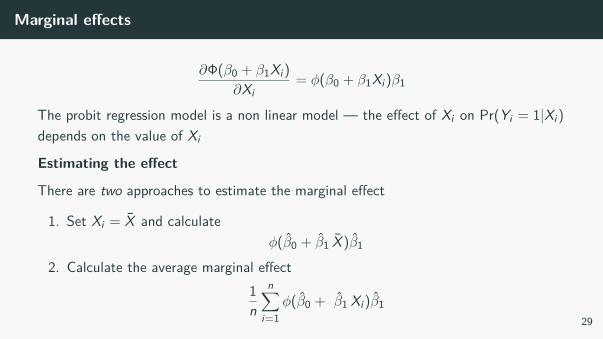
Marginal effects

∂Φ(β0 + β1Xi )∂Xi

= φ(β0 + β1Xi )β1

The probit regression model is a non linear model — the effect of Xi on Pr(Yi = 1|Xi )depends on the value of Xi

Estimating the effect

There are two approaches to estimate the marginal effect

1. Set Xi = X and calculateφ(β0 + β1 X )β1

2. Calculate the average marginal effect1n

n∑i=1

φ(β0 + β1 Xi )β129

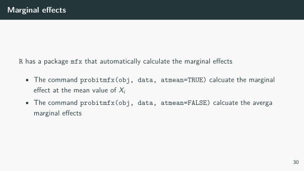
Marginal effects

R has a package mfx that automatically calculate the marginal effects

• The command probitmfx(obj, data, atmean=TRUE) calcuate the marginaleffect at the mean value of Xi

• The command probitmfx(obj, data, atmean=FALSE) calcuate the avergamarginal effects

30

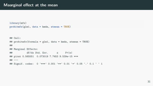
Maarginal effect at the mean

library(mfx)probitmfx(glm1, data = hmda, atmean = TRUE)

## Call:## probitmfx(formula = glm1, data = hmda, atmean = TRUE)#### Marginal Effects:## dF/dx Std. Err. z P>|z|## pirat 0.565551 0.073019 7.7453 9.539e-15 ***## ---## Signif. codes: 0 '***' 0.001 '**' 0.01 '*' 0.05 '.' 0.1 ' ' 1

31

Average Marginal effect

probitmfx(glm1, data = hmda, atmean = FALSE)

## Call:## probitmfx(formula = glm1, data = hmda, atmean = FALSE)#### Marginal Effects:## dF/dx Std. Err. z P>|z|## pirat 0.566748 0.073145 7.7483 9.312e-15 ***## ---## Signif. codes: 0 '***' 0.001 '**' 0.01 '*' 0.05 '.' 0.1 ' ' 1

32

What about discrimination

glm1 <- glm(deny ~ pirat + afam, data = hmda, family = binomial(probit))summary_rob(glm1)

#### Coefficients:## Estimate Std. Error z value Pr(>|z|)## (Intercept) -2.25877 0.17660 -12.790 < 2e-16## pirat 2.74174 0.49765 5.509 3.6e-08## afam 0.70816 0.08309 8.523 < 2e-16## ---## Heteroskadasticity robust standard errors used#### Multiple R-squared: , Adjusted R-squared:## F-statistic: 111.3 on 2 and Inf DF, p-value: < 2.2e-16

33

What about discrimination

probitmfx(glm1, atmean = FALSE, data = hmda)

## Call:## probitmfx(formula = glm1, data = hmda, atmean = FALSE)#### Marginal Effects:## dF/dx Std. Err. z P>|z|## pirat 0.501624 0.069043 7.2654 3.720e-13 ***## afam 0.169664 0.024254 6.9954 2.644e-12 ***## ---## Signif. codes: 0 '***' 0.001 '**' 0.01 '*' 0.05 '.' 0.1 ' ' 1#### dF/dx is for discrete change for the following variables:#### [1] "afam"

34

Logit Regression

Logit regression models the probability of Y=1 as the cumulative standard logisticdistribution function, evaluated at β0 + β1X :

Pr(Y = 1|X ) = F (β0 + β1X )

• F is the cumulative logistic distribution function:

F (β0 + β1X ) = 11 + e−(β0+β1X)

35

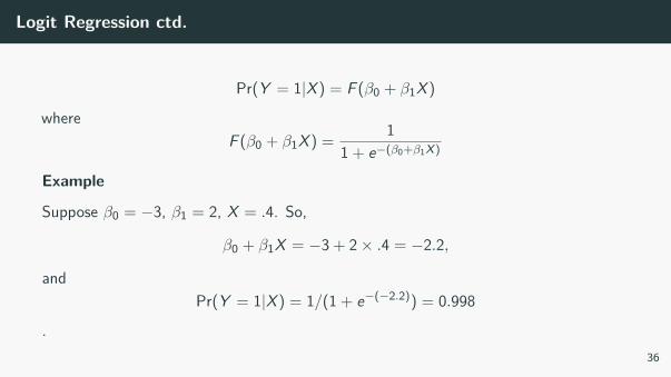
Logit Regression ctd.

Pr(Y = 1|X ) = F (β0 + β1X )

whereF (β0 + β1X ) = 1

1 + e−(β0+β1X)

Example

Suppose β0 = −3, β1 = 2, X = .4. So,

β0 + β1X = −3 + 2× .4 = −2.2,

andPr(Y = 1|X ) = 1/(1 + e−(−2.2)) = 0.998

.36

Logit Regression

Why bother with logit if we have probit?

• Historically, logit is more convenient computationally• In practice, logit and probit are very similar

37

Logit is very convinient

P(Y = 1|X1, . . . ,Xk) = 11 + expβ0 + β1X1 + . . .+ βkXk

impliesP(Y = 0|X1, . . . ,Xk) = expβ0 + β1X1 + . . .+ βkXk

1 + expβ0 + β1X1 + . . .+ βkXk

impliesP(Y = 0|X1, . . . ,Xk)P(Y = 1|X1, . . . ,Xk) = exp(β0 + β1X1 + · · ·+ βkXk)

38

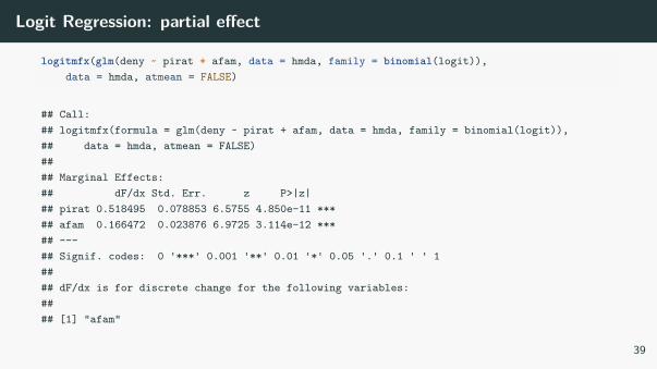
Logit Regression: partial effect

logitmfx(glm(deny ~ pirat + afam, data = hmda, family = binomial(logit)),data = hmda, atmean = FALSE)

## Call:## logitmfx(formula = glm(deny ~ pirat + afam, data = hmda, family = binomial(logit)),## data = hmda, atmean = FALSE)#### Marginal Effects:## dF/dx Std. Err. z P>|z|## pirat 0.518495 0.078853 6.5755 4.850e-11 ***## afam 0.166472 0.023876 6.9725 3.114e-12 ***## ---## Signif. codes: 0 '***' 0.001 '**' 0.01 '*' 0.05 '.' 0.1 ' ' 1#### dF/dx is for discrete change for the following variables:#### [1] "afam"

39

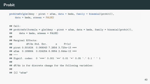
Probit

probitmfx(glm(deny ~ pirat + afam, data = hmda, family = binomial(probit)),data = hmda, atmean = FALSE)

## Call:## probitmfx(formula = glm(deny ~ pirat + afam, data = hmda, family = binomial(probit)),## data = hmda, atmean = FALSE)#### Marginal Effects:## dF/dx Std. Err. z P>|z|## pirat 0.501624 0.069043 7.2654 3.720e-13 ***## afam 0.169664 0.024254 6.9954 2.644e-12 ***## ---## Signif. codes: 0 '***' 0.001 '**' 0.01 '*' 0.05 '.' 0.1 ' ' 1#### dF/dx is for discrete change for the following variables:#### [1] "afam"

40

LPM

summary_rob(lm(ndeny ~ pirat + afam, data = hmda))

#### Coefficients:## Estimate Std. Error z value Pr(>|z|)## (Intercept) -0.11575 0.02901 -3.990 6.60e-05## pirat 0.63744 0.09067 7.030 2.06e-12## afam 0.17520 0.02491 7.033 2.02e-12## ---## Heteroskadasticity robust standard errors used#### Residual standard error: 0.312 on 2376 degrees of freedom## Multiple R-squared: 0.07501, Adjusted R-squared: 0.07423## F-statistic: 108.2 on 2 and Inf DF, p-value: < 2.2e-16

41

Example: Characterizing the Background of Hezbollah Militants

Source: Alan Krueger and Jitka Maleckova, “Education, Poverty and Terrorism: IsThere a Causal Connection?” Journal of Economic Perspectives, Fall 2003, 119-144

42

Example: Characterizing the Background of Hezbollah Militants

!

Figure 2: 43

Example: Characterizing the Background of Hezbollah Militants

!

Figure 3: 44

Example: Characterizing the Background of Hezbollah Militants

Pr(Y = 1|secondary = 1, poverty = 0, age = 20)− Pr(Y = 1|secondary = 1, poverty = 0, age = 20)

= .000646− .000488 = .000158

Both these statements are true:

• The probability of being a Hezbollah militant increases by 0.0158 percentage point,if secondary school is attended.

• The probability of being a Hezbollah militant increases by 32%, if secondary schoolis attended (.000158/.000488 = .32).

45

Logit and Probit: Estimation and Inference

• Logit and Probit coefficients are estimated through Maximum likelihood• Once the coefficients are estimated, R gives you all the information to carry out

inference on the parameters (confidence intervals, testing, etc.)• What happens if the X of the probit model is expressed in logarithm? And if X is a

dummy variable?

46