28 Boundary layers Between the two extremes of sluggish creeping flow at low Reynolds number and lively ideal flow at high, there is a regime in which neither is dominant. At large Reynolds number, the flow will be nearly ideal almost everywhere, except near solid boundaries where the no- slip condition requires the speed of the fluid to match the speed of the boundary wall. Here transition layers will arise in which the flow velocity changes rapidly from the velocity of the wall to the velocity of the flow in the fluid at large. Boundary layers are typically thin compared to the radii of curvature of the solid walls, and that simplifies the basic equations. In a boundary layer the character of the flow thus changes from creeping near the boundary to ideal well outside. The most interesting and also most difficult physics characteristically takes place in such transition regions. But humans live out their lives in nearly ideal flows of air and water at Reynolds numbers in the millions with boundary layers only millimeters thick, and are normally not conscious of them. Smaller animals eking out an existence at the surface of a stone in a river may be much more aware of the vagaries of boundary layer physics which may influence their body shapes and internal layout of organs. Ludwig Prandtl (1875–1953). German physicist, often called the father of aerodynamics. Con- tributed to wing theory, stream- lining, compressible subsonic air- flow and turbulence. Boundary layers serve to insulate bodies from the ideal flow that surrounds them. They have a ‘life of their own’ and may separate from the solid walls and wander into regions con- taining only fluid. Detached layers may again split up, creating complicated unsteady patterns of whirls and eddies. Advanced understanding of fluid mechanics begins with an understand- ing of boundary layers. Systematic boundary layer theory was initiated by Prandtl in 1904 and has in the twentieth century become a major subtopic of fluid mechanics [Schlichting and Gersten 2000, Sobey 2000, White 1991]. In this chapter we shall mainly focus on the theory of incompressible laminar boundary layers without heat flow. 28.1 Physics of boundary layers q q q q q q q q q . . . . . U . . . .. . . . . . . . . . . . . . . . . . . . ı The transition from zero velocity at the wall to the mainstream ve- locity U mostly takes place in a layer of finite thickness ı. The no-slip condition forces the velocity of a fluid to vanish at a static solid wall. Under many—but not all—circumstances, the transition between the rapid flow at high Reynolds number in the fluid at large and the stagnation at the wall will take place in a thin boundary layer hugging the wall. Close to the wall, the velocity field is so small that the flow pattern will always be laminar, in fact creeping, with the velocity field rising linearly from zero. The laminar flow may extend all the way to the edge of the boundary layer, or it may become turbulent if the Reynolds number is sufficiently large. Copyright c 1998–2010 Benny Lautrup
Transcript
28Boundary layers
Between the two extremes of sluggish creeping flow at low Reynolds number and lively idealflow at high, there is a regime in which neither is dominant. At large Reynolds number,the flow will be nearly ideal almost everywhere, except near solid boundaries where the no-slip condition requires the speed of the fluid to match the speed of the boundary wall. Heretransition layers will arise in which the flow velocity changes rapidly from the velocity ofthe wall to the velocity of the flow in the fluid at large. Boundary layers are typically thincompared to the radii of curvature of the solid walls, and that simplifies the basic equations.
In a boundary layer the character of the flow thus changes from creeping near the boundaryto ideal well outside. The most interesting and also most difficult physics characteristicallytakes place in such transition regions. But humans live out their lives in nearly ideal flowsof air and water at Reynolds numbers in the millions with boundary layers only millimetersthick, and are normally not conscious of them. Smaller animals eking out an existence atthe surface of a stone in a river may be much more aware of the vagaries of boundary layerphysics which may influence their body shapes and internal layout of organs.
Ludwig Prandtl (1875–1953).German physicist, often calledthe father of aerodynamics. Con-tributed to wing theory, stream-lining, compressible subsonic air-flow and turbulence.
Boundary layers serve to insulate bodies from the ideal flow that surrounds them. Theyhave a ‘life of their own’ and may separate from the solid walls and wander into regions con-taining only fluid. Detached layers may again split up, creating complicated unsteady patternsof whirls and eddies. Advanced understanding of fluid mechanics begins with an understand-ing of boundary layers. Systematic boundary layer theory was initiated by Prandtl in 1904 andhas in the twentieth century become a major subtopic of fluid mechanics [Schlichting and Gersten 2000,Sobey 2000, White 1991].
In this chapter we shall mainly focus on the theory of incompressible laminar boundarylayers without heat flow.
The transition from zero velocityat the wall to the mainstream ve-locity U mostly takes place in alayer of finite thickness ı.
The no-slip condition forces the velocity of a fluid to vanish at a static solid wall. Undermany—but not all—circumstances, the transition between the rapid flow at high Reynoldsnumber in the fluid at large and the stagnation at the wall will take place in a thin boundarylayer hugging the wall. Close to the wall, the velocity field is so small that the flow patternwill always be laminar, in fact creeping, with the velocity field rising linearly from zero. Thelaminar flow may extend all the way to the edge of the boundary layer, or it may becometurbulent if the Reynolds number is sufficiently large.
Copyright c 1998–2010 Benny Lautrup
476 PHYSICS OF CONTINUOUS MATTER
Laminar boundary layer thicknessDenoting the typical velocity of the mainstream flow by U , the Reynolds number is as usualRe � UL=� where L is the length scale for significant changes in the flow, determined bythe geometry of bodies and containers. We shall always assume that it is large, Re� 1. Theeffective Reynolds number in a steady laminar boundary layer of thickness ı can be estimatedfrom the ratio of advective to viscous terms in the Navier–Stokes equation,
j.v � r/vj
j�r2vj�U 2=L
�U=ı2Dı2
L2Re: (28.1)
Here the numerator is estimated from the change in mainstream velocity along the wall overa distance L, using that the flow in a laminar layer must follow the geometry of the body.The denominator is estimated from the rapid change in velocity across the thickness ı of theboundary layer.
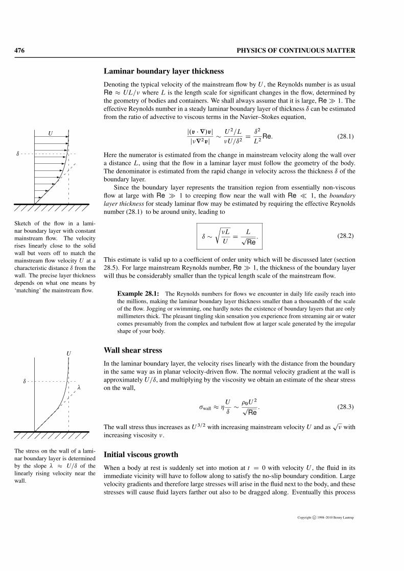
Sketch of the flow in a lami-nar boundary layer with constantmainstream flow. The velocityrises linearly close to the solidwall but veers off to match themainstream flow velocity U at acharacteristic distance ı from thewall. The precise layer thicknessdepends on what one means by‘matching’ the mainstream flow.
Since the boundary layer represents the transition region from essentially non-viscousflow at large with Re � 1 to creeping flow near the wall with Re � 1, the boundarylayer thickness for steady laminar flow may be estimated by requiring the effective Reynoldsnumber (28.1) to be around unity, leading to
ı �
r�L
UD
Lp
Re: (28.2)
This estimate is valid up to a coefficient of order unity which will be discussed later (section28.5). For large mainstream Reynolds number, Re � 1, the thickness of the boundary layerwill thus be considerably smaller than the typical length scale of the mainstream flow.
Example 28.1: The Reynolds numbers for flows we encounter in daily life easily reach intothe millions, making the laminar boundary layer thickness smaller than a thousandth of the scaleof the flow. Jogging or swimming, one hardly notes the existence of boundary layers that are onlymillimeters thick. The pleasant tingling skin sensation you experience from streaming air or watercomes presumably from the complex and turbulent flow at larger scale generated by the irregularshape of your body.
The stress on the wall of a lami-nar boundary layer is determinedby the slope � � U=ı of thelinearly rising velocity near thewall.
In the laminar boundary layer, the velocity rises linearly with the distance from the boundaryin the same way as in planar velocity-driven flow. The normal velocity gradient at the wall isapproximately U=ı, and multiplying by the viscosity we obtain an estimate of the shear stresson the wall,
�wall � �U
ı��0U
2
pRe
: (28.3)
The wall stress thus increases as U 3=2 with increasing mainstream velocity U and asp� with
increasing viscosity �.
Initial viscous growthWhen a body at rest is suddenly set into motion at t D 0 with velocity U , the fluid in itsimmediate vicinity will have to follow along to satisfy the no-slip boundary condition. Largevelocity gradients and therefore large stresses will arise in the fluid next to the body, and thesestresses will cause fluid layers farther out also to be dragged along. Eventually this process
Copyright c 1998–2010 Benny Lautrup
28. BOUNDARY LAYERS 477
may come to an end and the flow will become steady. In the beginning the newly createdboundary layer is extremely thin, so that the general geometry of the flow and the shape ofthe body cannot matter. This indicates that suddenly created boundary layers always start outtheir growth in the same universal way.
The wall is suddenly set into mo-tion. After a time t , the veloc-ity of the fluid at the edge ofthe growing boundary layer haschanged from 0 to U .
To estimate the universal growth of the boundary layer thickness ı.t/, we use that at time tthe fluid at the edge of the boundary layer will have changed its velocity from 0 to U , makingthe local acceleration of order U=t . The ratio between the local and advective accelerationthen becomes,
j@v=@t j
j.v � r/vj�
U=t
U 2=LD
L
Ut: (28.4)
The time the fluid takes to pass the body is L=U . For times much shorter than this, t �L=U , the local acceleration dominates the advective acceleration term, and the boundarylayer will continue to grow. In a ‘young’ boundary layer the advective acceleration can thusbe disregarded, and the physics is controlled by the ratio of local to viscous acceleration,
j@v=@t j
j�r2vj�
U=t
�U=ı2Dı2
�t: (28.5)
Requiring this to be of order unity, we find for t � L=U ,
ı �p�t : (28.6)
A suddenly created boundary layer always starts out like this, growing with the square root oftime. This behaviour is typical of viscous diffusion processes (page 231).
Initial growth of a laminar bound-ary layer. The three velocityprofiles correspond to increasingtimes t1 < t2 < t3 and increas-ing thicknesses ı1 < ı2 < ı3.
After the initial universal growth, the boundary layer comes to depend on the generalgeometry of the flow for t � L=U , when the estimate reaches the steady layer thickness(28.2) . It takes more careful analysis to see whether the flow eventually ‘goes steady’, orwhether instabilities arise, leading to a radical change in the character of the flow, such asboundary layer separation or turbulence.
A semi-infinite plate in an other-wise uniform flow. The dashedcurve is the estimated parabolicboundary layer shape.
The simplest geometry in which a steady boundary layer can be studied is a semi-infinite platewith its edge orthogonal to a uniform mainstream flow (solved analytically in section 28.5).Here the only possible length scale is the distance x from the leading edge, so we must have
ı �
r�x
U: (28.7)
This shows that the boundary layer grows thicker downstream, even if the mainstream flow iscompletely uniform and independent of x. Disregarding sound waves, the time t D x=U ittakes the flow to pass through the distance x is also the earliest moment that the leading edgecan causally influence the flow near x. Intuitively one might say that the universal viscousgrowth of the boundary layer is curtailed by the encounter with the blast of undisturbed fluidcoming in from afar.
Sketch of the boundary layeraround a bluff body in steadyuniform flow. On the windwardside the boundary layer is thin,whereas it widens and tends toseparate on the lee side. Inthe channel formed by the sep-arated boundary layer, unsteadyflow patterns may arise.
Boundary layers have a natural tendency towards downstream thickening, because theybuild up along a body in a cumulative fashion. Having reached a certain thickness, a boundarylayer acts as a not-quite-solid ‘wall’ on which another boundary layer will form. The thicknessof a steady boundary layer is also strongly dependent on whether the mainstream flow isaccelerating or decelerating along the body, behaviour which in turn is determined by thegeometry. If the mainstream flow accelerates, i.e. grows with x, the boundary layer tends toremain thin. This happens at the front of a moving body, where the fluid must speed up to get
Copyright c 1998–2010 Benny Lautrup
478 PHYSICS OF CONTINUOUS MATTER
out of the way. Conversely, towards the rear of the body, where the mainstream flow againdecelerates in order to ‘fill up the hole’ left by the passing body, the boundary layer becomesrapidly thicker, and may even separate from the body, creating an unsteady, even turbulent,trailing wake. The von Karman vortex street (page 460) is an example of periodic unsteadyflow in the wake of a body.
Merging boundary layers
The increase of a boundary layer’s thickness with downstream distance implies that the bound-ary layer around an infinite body must become infinitely thick or at least so thick that it fillsout all the available space. In steady planar flow between moving plates (section 14.1), wesaw that the velocity profile of the fluid interpolates linearly between the plate velocities,and there is nothing like a boundary layer with finite thickness near the plates. Likewise, inpressure-driven steady planar flow or pipe flow (sections 15.2 and 15.4), the exact shape ofthe velocity profile is parabolic (as long as the flow is laminar), whatever the viscosity of thefluid. Again we see no trace of a finite boundary layer in the exact solutions. Completelymerged boundary layers are, however, only found in infinite systems. In a pipe of finite lengththe boundary layers grow out from the walls, starting at the entrance to the pipe and eventuallymerge at a distance, called the entrance length, which we estimated on page 252.
The thickening of a boundarylayer decelerates the flow andleads to upwelling of fluid fromthe boundary.
Inside a boundary layer, at a fixed distance from a flat solid wall with a uniform mainstreamvelocity U , the flow decelerates downstream as the boundary layer thickens due to the actionof viscosity. Mass conservation requires a compensating upwelling of fluid into the fluid atlarge. If, on the other hand, the boundary is permeable and fluid is sucked down through it ata constant rate, the upflow can be avoided, and a steady boundary layer of constant thicknessmay be created (problem 28.1).
The mainstream flow is determined by bodies and containers that guide the fluid and willgenerally not be uniform but rather accelerate or decelerate along the boundaries. An acceler-ating mainstream flow will counteract the natural deceleration in the boundary layer and mayeven overwhelm it, leading to a downwash towards the boundary. Mainstream accelerationthus tends to stabilize a boundary layer so that it has less tendency to thicken, and may lead toconstant or even diminishing thickness. Conversely, if the mainstream flow decelerates, thiswill add to the natural deceleration in the boundary layer and increase its thickness as well asthe upwelling.
Velocity profiles before and af-ter the separation point (dashedline).
Even at very moderate mainstream deceleration, the upwelling can become so strong that atsome point the fluid flowing in the mainstream direction cannot feed it. Some of the fluid inthe boundary layer will then have to flow against the mainstream flow. Between the forwardand reversed flows there will be a separation line ending in a stagnation point on the wall.Such flow reversal was also noted in lubrication (page 281), although there are no boundarylayers in creeping flow.
In the region of reversed flow, the velocity still has to vanish right at the boundary. Movingup from the boundary wall, the flow first moves backwards with respect to the mainstream, butfarther from the wall it must again turn back to join up with the mainstream. The velocity gra-dient must accordingly be negative right at the boundary in the reversal region, correspondingto a negative wall stress �wall. At the separation point the wall stress must necessarily vanish,but flow reversal can in principle take place entirely within the boundary layer without properseparation, for example at a dent in the wall.
Copyright c 1998–2010 Benny Lautrup
28. BOUNDARY LAYERS 479
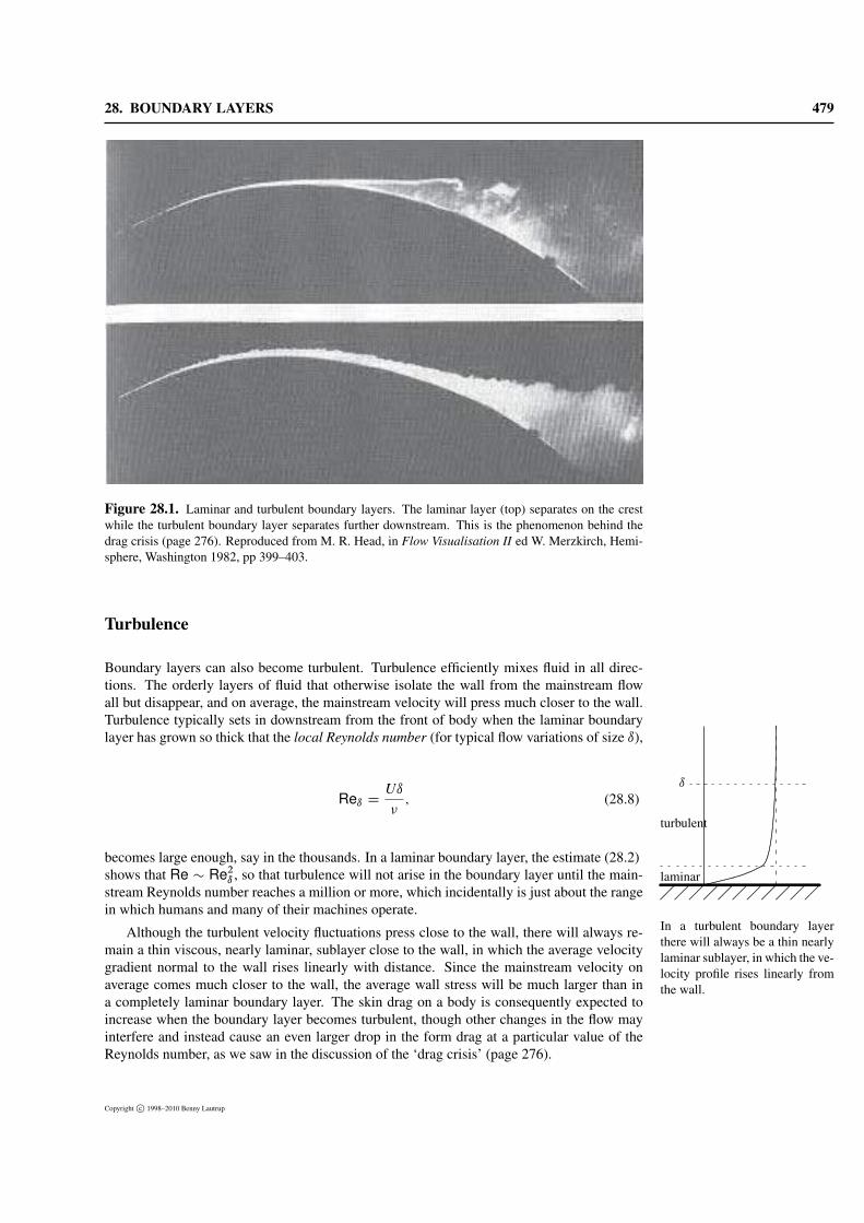
Figure 28.1. Laminar and turbulent boundary layers. The laminar layer (top) separates on the crestwhile the turbulent boundary layer separates further downstream. This is the phenomenon behind thedrag crisis (page 276). Reproduced from M. R. Head, in Flow Visualisation II ed W. Merzkirch, Hemi-sphere, Washington 1982, pp 399–403.
Turbulence
Boundary layers can also become turbulent. Turbulence efficiently mixes fluid in all direc-tions. The orderly layers of fluid that otherwise isolate the wall from the mainstream flowall but disappear, and on average, the mainstream velocity will press much closer to the wall.Turbulence typically sets in downstream from the front of body when the laminar boundarylayer has grown so thick that the local Reynolds number (for typical flow variations of size ı),
Reı DUı
�; (28.8)
becomes large enough, say in the thousands. In a laminar boundary layer, the estimate (28.2)shows that Re � Re2ı , so that turbulence will not arise in the boundary layer until the main-stream Reynolds number reaches a million or more, which incidentally is just about the rangein which humans and many of their machines operate.
In a turbulent boundary layerthere will always be a thin nearlylaminar sublayer, in which the ve-locity profile rises linearly fromthe wall.
Although the turbulent velocity fluctuations press close to the wall, there will always re-main a thin viscous, nearly laminar, sublayer close to the wall, in which the average velocitygradient normal to the wall rises linearly with distance. Since the mainstream velocity onaverage comes much closer to the wall, the average wall stress will be much larger than ina completely laminar boundary layer. The skin drag on a body is consequently expected toincrease when the boundary layer becomes turbulent, though other changes in the flow mayinterfere and instead cause an even larger drop in the form drag at a particular value of theReynolds number, as we saw in the discussion of the ‘drag crisis’ (page 276).
Copyright c 1998–2010 Benny Lautrup
480 PHYSICS OF CONTINUOUS MATTER
28.2 The Stokes layerThe initial growth of the boundary layer at a flat plate suddenly set into motion (Stokes firstproblem) must also follow the universal law (28.6) . In this case there is no intrinsic lengthscale for the geometry, and the transition to geometry-dependent steady flow cannot takeplace. The planar boundary layer, called the Stokes layer, can for this reason be expected toprovide a clean model for the universal viscous growth.
Analytic solutionAs usual it is best to view the system from the reference frame in which the plate and the fluidinitially move with the same velocity U and the plate is suddenly stopped at t D 0. Assumingthat the flow is planar with vx D vx.y; t/ and vy D 0, the Navier–Stokes equation forincompressible flow reduces to the momentum-diffusion equation (14.5) , which is repeatedhere for convenience
@vx
@tD �
@2vx
@y2: (28.9)
The linearity of this equation guarantees that the velocity everywhere must be proportionalto U , and since there is no intrinsic length or time scale in the definition of the problem, thevelocity field must be of the form,
vx.y; t/ D Uf .s/; s Dy
2p�t: (28.10)
The so far unknown function f .s/ should obey the boundary conditions f .0/ D 0 andf .1/ D 1. The factor two in the denominator is just a convenient choice.
Upon insertion of (28.10) into (28.9) we are led to an ordinary second-order differentialequation for f .s/,
f 00.s/C 2sf 0.s/ D 0: (28.11)
Viewed as a first-order equation for f 0.s/, it has the unique solution f 0.s/ � exp.�s2/.Integrating this expression once more over s and applying the boundary conditions, the finalresult becomes
f .s/ D2p�
Z s
0
e�u2
du D erf.s/; (28.12)
where erf.�/ is the well-known error function, shown in figure 28.2(a).
Gaussian tailFor large values the error function approaches unity with a Gaussian tail, 1�f .s/ � exp.�s2/ Dexp.�y2=4�t/, typical of momentum diffusion. The Gaussian tail extends all the way tospatial infinity for any positive time, t > 0, but how can that be, when the plate was onlybrought to stop at time t D 0? Will it take a finite time for this event to propagate to spa-tial infinity? The short answer is that we have assumed the fluid to be incompressible, andthis—fundamentally untenable—assumption will in itself entail infinite signal speeds. At adeeper level, a diffusion equation like (28.9) is the statistical continuum limit of the dynamicsof random molecular motion in the fluid, and although extremely high molecular speeds arestrongly damped, they may in principle occur. The effective limit to diffusion speed is, asdiscussed before, always set by the finite speed of sound.
Copyright c 1998–2010 Benny Lautrup
28. BOUNDARY LAYERS 481
Figure 28.2. (a) The Stokes layer shape function f .s/. The sloping dashed line is tangent at s D 0
with inclination f 0.0/ D 2=p� . (b) Detail near f .s/ D 1 in %.
Vorticity
The vorticity field has only one component
!z.y; t/ D �@vx.y; t/
@yD �
Uf 0.s/
2p�tD �
Up��t
e�y2=4�t : (28.13)
When the plate was still moving for t < 0, stopped, the flow was everywhere irrotational.Afterwards there is evidently vorticity everywhere in the boundary layer. Where did thatcome from?
-U
L
-
6
�
?
The circulation around an in-finitely tall rectangle with side Lagainst the moving wall is � DH
v � d` D �UL.
Consider a (nearly) infinite rectangle with support of length L on the plate. By Stokes’theorem the total flux of vorticity (or circulation) through the rectangle is � D
R! � dS DH
v � d`. The fluid velocity always vanishes on the plate, is orthogonal to the sides andapproaches the constant U at infinity, so that we obtain � D �UL. Since the circulation isconstant in time, vorticity is not generated inside the boundary layer itself during its growth,but rather at the plate surface during the instantaneous deceleration to zero velocity. If theplate did not stop with infinite deceleration, but followed a gentler road U.t/ from U to 0,the circulation �.t/ D .U.t/ � U/L would also have decreased gently from 0 to �UL.The conclusion is that vorticity is generated at the plate surface during the deceleration, andafterwards it diffuses away from the plate and into the fluid at large without changing the totalcirculation.
Thickness
The velocity field is self-similar because it only depends on the dimensionless variable s Dy=2p�t . At different times the velocity profiles only differ by the ‘vertical’ length scale
2p�t . There is no cut-off in the infinitely extended Gaussian tail and therefore no ‘true’
thickness ı. Conventionally, one defines the boundary layer thickness to be the distance wherethe velocity has reached 99% of the terminal velocity. The solution to f .s/ D 0:99 is s D1:82 : : : (see figure 28.2(b)), such that
ı99 D 1:82 : : : � 2p�t � 3:64
p�t : (28.14)
In section 28.8 we shall meet other more physical definitions of boundary layer thickness.
Copyright c 1998–2010 Benny Lautrup
482 PHYSICS OF CONTINUOUS MATTER
28.3 Advective cooling or heating
When you take a walk on a cold day, your heat loss is amplified by wind which removes thewarm air near your body and creates a large temperature gradient at the surface of the skin,resulting in a larger conductive heat transfer from your body to the air. In meteorology thisis known as wind chill, and the local ‘wind chill temperature’ is often announced by weatherforecasters during winter. A similar phenomenon must of course occur in a hot desert wind,although the local ‘wind burn’ is not a regular part of a summer weather forecast. In a saunawith air at 120 ı C, it is well known that one should not move around too fast.
Fur coats or wet suits: Somewhat surprisingly, the heat diffusivity of air at rest (31 �10�6 m2=s) turns out to be about 200 times larger than that of water (0:14 � 10�6 m2=s). Whyis it then that we use air for insulation in thermoglass windows, bed covers and fur coats—ratherthan sleeping and walking in wet suits? The explanation is that although heat diffuses much fasterin air than in water, the actual heat current (22.17) is—for a given temperature gradient—not de-termined by the diffusivity but by the thermal conductivity which is about 23 times larger in waterthan in air. Consequently, you lose much less heat in a fur coat than in a wet suit, even if the lowtemperature penetrates the fur coat much faster. The role of fur coats or wet suits is mainly to pre-vent advection of heat by air or water currents which will rapidly remove the warm fluid adjacentto your skin, thereby increasing the temperature gradient at the skin and thus the heat flow fromyour body.
Water chill is even more important. A cold water current moving with the same speed andtemperature as a cold wind results in much stronger cooling because of the 25 times higherthermal conductivity of water. This is why you are only able to survive naked for minutes instreaming water at 0 ı C whereas you may survive for hours in a wind of that temperature.Similarly, hot water scalds you much faster than hot air of the same temperature.
In this section we shall discuss the limit where the temperature does not influence themotion of the fluid. In that case the flow of heat takes place against the background of a massflow, completely controlled by the external forces that drive the fluid. This limit is often calledthe limit of forced convection to distinguish it from the opposite limit, free convection, wherethe motion of the fluid is entirely caused by temperature differences (to be discussed at lengthin chapter 30).
Advective cooling of a plate withwind coming in from the left. Theboundary for the mass flow (solidline) and the heat fronts (dashed)for large and small Prandtl num-bers.
Advective cooling (or heating) of the surface of a body involves both momentum and heatdiffusion along the normal to the surface. In a time t after the start of the flow, momentumdiffusion reaches a characteristic distance ımass �
p�t from the surface whereas heat dif-
fusion reaches ıheat �p�t . The ratio between momentum and heat diffusivities is for this
reason an important dimensionless quantity, called the Prandtl number,
Pr D�
�: (28.15)
When the Prandtl number is large, temperature variations will take place well inside the usualboundary layer, whereas if the Prandtl number is small, the temperature distribution spreadswell beyond the boundary layer.
In contrast to other dimensionless numbers, for example the Reynolds or Peclet numbers, thePrandtl number is a property of the fluid rather than of the flow. In gases it is of order unity, forexample Pr D 0:73 for air at normal temperature and pressure. In liquids it may take a wide rangeof values: in water it is about 6, whereas in liquid metals it is quite small, for example 0:025 formercury. For isolating liquids like oil it may be quite large, of the order of 1000.
Copyright c 1998–2010 Benny Lautrup
28. BOUNDARY LAYERS 483
Wind chill estimateIn a steady flow with velocity scale U boundary layers will stop growing after the time t �L=U it takes for the fluid to move across the downstream length L of the body. The scaleof the heat boundary layer thickness thus becomes ıheat �
p�L=U , and the temperature
gradient at the surface is expected to be jrT j � ‚=ıheat, where ‚ is the temperature excessof the body relative to the fluid at large. From Fourier’s law (22.17) we estimate that the rateof loss of heat from a body surface of area A is,
PQ � k‚
ıheatA � k‚A
rU
�L: (28.16)
We shall show below in an exact calculation that this is indeed of the right form.The main consequence of the above estimate is that the heat loss grows with the squareroot
of the velocity, thus confirming the observation that a higher velocity has the same effect as alarger temperature excess. Let the actual temperature excess be ‚ D T0 � T where T0 is theexposed surface temperature and T is the wind temperature, and let the actual wind velocitybe U . Then the heat loss will be the same for a temperature excess‚� D T0�T � and a windspeed U �, provided‚�
pU � D ‚
pU . Solving for the fictive wind temperature T � we find,
Paul Allen Siple (1908-68).American Antarctic explorer.Accompanied (as an EagleScout) the first Byrd expedi-tion to Antarctica in 1928-30.Participated in Byrd’s secondexpedition 1933-35 as a chief bi-ologist. Coined the term “windchill” in 1939.
T � D T0 � .T0 � T /
rU
U �: (28.17)
This is the essential part of the first wind chill formula by Siple and Passel (1945), who —after measuring cooling rates of water in plastic containers — arrived at the following slightlymodified empirical expression for the fictive temperature,
T � D T0 � .T0 � T /
rU
U �C 0:47 � 0:22
U
U �
!: (28.18)
The parameters were chosen to be T0 � 33ıC and U � � 5 m=s1. When the value of theexpression in the parenthesis equals unity, we have T � D T so that there is no wind chilleffect. This happens for U D 0:37U � � 1:85 m=s, roughly the speed of a walking human,which is quite reasonable. The formula makes no sense for lower speeds, because the fictivetemperature then will be higher than the wind temperature.
Example 28.2: At 0ıC a wind speed of U D 10m=s corresponds to a fictive wind temperatureof T � � �14ıC according to (28.18) . The modern formula yields instead T � � �7ıC.
Heat flow in the Blasius boundary layerThe simplest model of advective cooling is furnished by the steady-flow Blasius boundarylayer discussed in section 28.5 on page 487, with the added condition that the plate is held at aconstant temperature T D T0C‚ which is different from the ambient temperature T0. Sinceby assumption the mass flow is not influenced by the heat flow we may take the exact Blasiussolution and insert it into the steady flow heat equation,
.v � r/T D �r2T: (28.19)
In the boundary layer approximation the double derivativer2x can be disregarded in the Lapla-cian, so that the equation takes the same form as the Prandtl equation (28.33)
vx@T
@xC vy
@T
@yD �
@2T
@y2: (28.20)
1The Siple-Passel formula was used by the US National Weather Service from 1973 but became in2001 replaced by a somewhat more conservative expression based on modern theory and experiments. Seehttp://www.nws.noaa.gov/om/windchill .
Copyright c 1998–2010 Benny Lautrup
484 PHYSICS OF CONTINUOUS MATTER
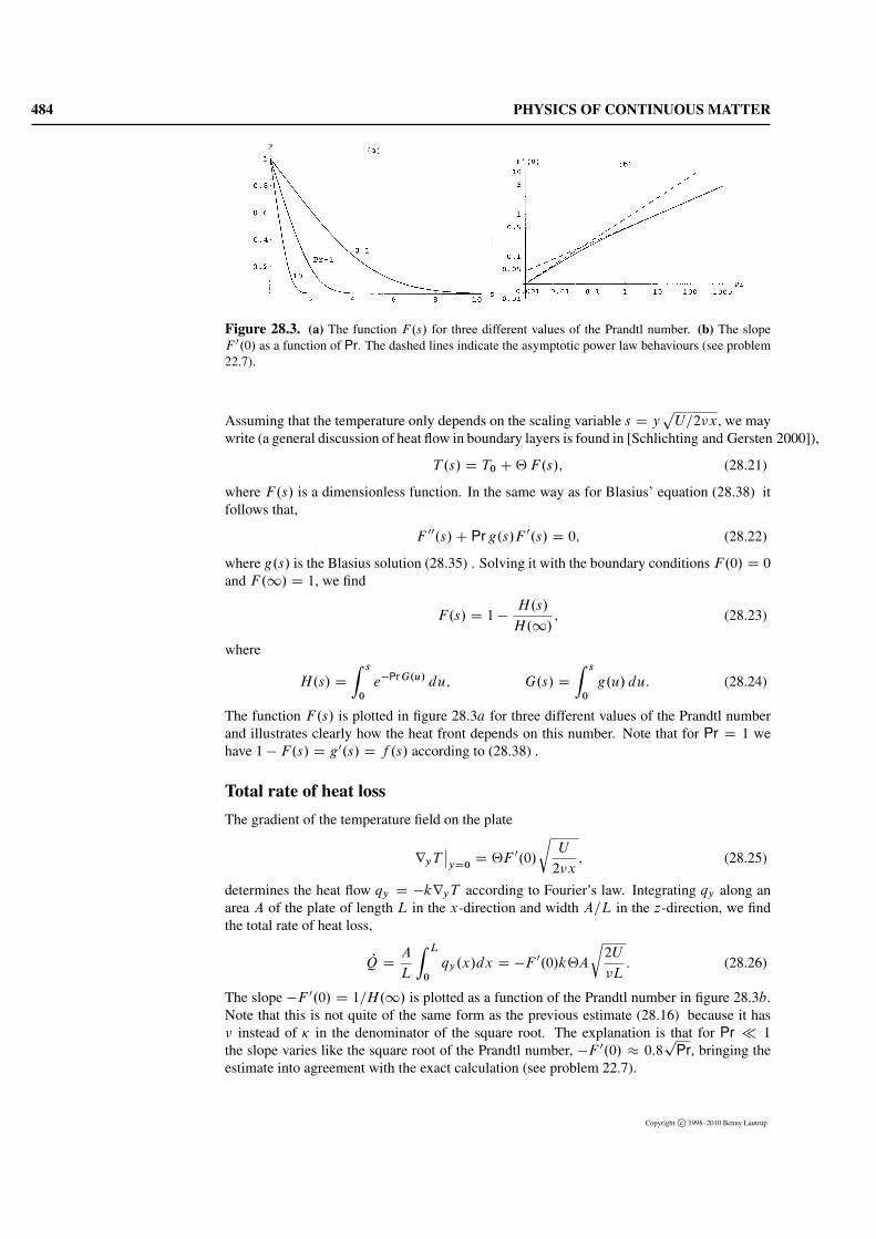
Figure 28.3. (a) The function F.s/ for three different values of the Prandtl number. (b) The slopeF 0.0/ as a function of Pr. The dashed lines indicate the asymptotic power law behaviours (see problem22.7).
Assuming that the temperature only depends on the scaling variable s D ypU=2�x, we may
write (a general discussion of heat flow in boundary layers is found in [Schlichting and Gersten 2000]),
T .s/ D T0 C‚F.s/; (28.21)
where F.s/ is a dimensionless function. In the same way as for Blasius’ equation (28.38) itfollows that,
F 00.s/C Prg.s/F 0.s/ D 0; (28.22)
where g.s/ is the Blasius solution (28.35) . Solving it with the boundary conditions F.0/ D 0and F.1/ D 1, we find
F.s/ D 1 �H.s/
H.1/; (28.23)
where
H.s/ D
Z s
0
e�PrG.u/ du; G.s/ D
Z s
0
g.u/ du: (28.24)
The function F.s/ is plotted in figure 28.3a for three different values of the Prandtl numberand illustrates clearly how the heat front depends on this number. Note that for Pr D 1 wehave 1 � F.s/ D g0.s/ D f .s/ according to (28.38) .
Total rate of heat lossThe gradient of the temperature field on the plate
ryTˇyD0D ‚F 0.0/
rU
2�x; (28.25)
determines the heat flow qy D �kryT according to Fourier’s law. Integrating qy along anarea A of the plate of length L in the x-direction and width A=L in the z-direction, we findthe total rate of heat loss,
PQ DA
L
Z L
0
qy.x/dx D �F0.0/k‚A
r2U
�L: (28.26)
The slope �F 0.0/ D 1=H.1/ is plotted as a function of the Prandtl number in figure 28.3b.Note that this is not quite of the same form as the previous estimate (28.16) because it has� instead of � in the denominator of the square root. The explanation is that for Pr � 1
the slope varies like the square root of the Prandtl number, �F 0.0/ � 0:8p
Pr, bringing theestimate into agreement with the exact calculation (see problem 22.7).
Copyright c 1998–2010 Benny Lautrup
28. BOUNDARY LAYERS 485
Example 28.3 [Human heat loss]: The grown-up human body has a skin surface area ofabout A � 2 m2. A naked human standing with shoulders aligned with the wind will roughlypresent a (two-sided) plate area with L � 0:5 m and A=L � 4 m. For air with Pr D 0:73 wehave �F 0.0/ D 0:42, so that in a wind with U D 1 m s�1 and a temperature ‚ D 10 K belowthe skin temperature we find the heat loss rate PQ � 100 W. Since the human body produces heatat this rate, a skin temperature of 27 ı C can thus be maintained essentially indefinitely in a gentlebreeze with velocity 1 m s�1 and temperature 17 ı C, not unlike what you find on a Scandinavianbeach on a summer day. In this calculation we have ignored natural convection and evaporativeheat losses.
Under the same conditions in water where �F 0.0/ D 0:87 the rate of heat loss becomesenormous, PQ � 23 kW, and will almost instantly cool the skin to the temperature of the water.Everybody is familiar with the (relatively mild) skin shock that is experienced when one jumpsinto water as warm as 17 ı C. At this temperature the loss of heat will eventually lead to severehypothermia and death in the course of some hours, depending on what you wear and how youbehave.
Geometry of two-dimensionalplanar boundary flow. In the ab-sence of viscosity there would bea slowly varying slip-flow U.x/
along the boundary. Viscosity in-terposes a thin boundary layer ofthickness ı.x/ between the slip-flow and the boundary.
When Prandtl introduced the concept of boundary layers he pointed out that there were sim-plifying features, allowing for less complicated equations. The greater simplicity comes fromthe assumption of nearly ideal mainstream flow with Re � 1, which according to the esti-mate (28.2) implies that boundary layers are thin, i.e. ı � L where L is the length scale forvariations in the mainstream flow.
We shall—as Prandtl did—consider only the two-dimensional case with an infinitely ex-tended planar boundary wall at y D 0 and a unidirectional mainstream flow along x. In theabsence of viscosity, the incompressible fluid would slip along the boundary, y D 0, witha slowly varying slip-velocity, vx D U.x/. Leaving out gravity, it follows from Bernoulli’stheorem (13.5) that there must be an associated slip-flow pressure at the boundary,
P.x/ D P0 �12�0U.x/
2; (28.27)
where P0 is a constant. The slip-flow pressure simply reflects the variation in slip-velocityalong the boundary.
The Prandtl equationsIn viscous flow the no-slip condition demands that the true velocity must change rapidly fromvx D 0 right at the boundary y D 0 to vx D U.x/ outside the boundary layer y � ı.Formulated more carefully, the slip-flow velocity U.x/ and boundary pressure P.x/ shouldnow be understood as describing the flow in the region ı � y � L, well outside the boundarylayer but still so close to the boundary that the mainstream flow depends mainly on x. Inthe mainstream proper, for y & L, flow and pressure come to depend on the general flowgeometry with other length scales for major flow variations along both x and y.
The continuity equation,
@vx
@xC@vy
@yD 0 (28.28)
determines the upflow vy both inside and outside the boundary layer. Integrating over y, andusing the boundary condition vy D 0 for y D 0, we obtain the exact relation,
vy.x; y/ D �@
@x
Z y
0
vx.x; y0/ dy0: (28.29)
Copyright c 1998–2010 Benny Lautrup
486 PHYSICS OF CONTINUOUS MATTER
Since major flow variations take place on the length scales L along x and ı along y, thisequation permits us to estimate the upflow to be of magnitude vy � U ı=L � U=
pRe. The
upflow inside the boundary layer will thus for Re� 1 be much smaller than the slip-flow.Mass conservation implies that the upflow inside the boundary layer continues into the
slip-flow region ı � y � L. Writing vx D U � .U � vx/ in (28.29) we obtain,
vy.x; y/ � �ydU.x/
dxCdQ.x/
dxfor ı � y � L; (28.30)
where
Q.x/ D
Z y
0
.U.x/ � vx.x; y// dy �
Z L
0
.U.x/ � vx.x; y// dy: (28.31)
In the last step we have replaced the upper limit y by L under the assumption that U � vxvanishes rapidly outside the boundary layer for y & ı.
The quantityQ.x/ represents the volume of the slip-flow displaced by the boundary layerper unit of time (and per unit of length along z). The upflow (28.30) in the slip-flow regionthus has two contributions, one from the variations in slip-flow and one from the boundarylayer itself. The latter represents the natural upwelling in the boundary layer discussed onpage 478.
In two dimensions the steady-flow Navier–Stokes equations (15.1) become
vx@vx
@xC vy
@vx
@yD �
1
�0
@p
@xC �
�@2vx
@x2C@2vx
@y2
�; (28.32a)
vx@vy
@xC vy
@vy
@yD �
1
�0
@p
@yC �
�@2vy
@x2C@2vy
@y2
�: (28.32b)
In either of these equations, the double derivative after y is proportional to 1=ı2, whereasthe double derivative after x is proportional to 1=L2, making it a factor 1=Re smaller andthus negligible for Re � 1. Setting vx � U and vy � Uı=L we estimate from any ofthe remaining terms in the second equation that the normal pressure gradient is @p=@y ��0U
2ı=L2. Finally, multiplying this expression with ı we obtain the pressure variation acrossthe boundary layer �yp � ı @p=@y � �0U
2ı2=L2 � �0U2=Re. For Re � 1 this is much
smaller than the typical variation in slip-flow pressure �P � �0U 2 and may be disregarded.In this approximation the true pressure in the boundary layer equals the slip-flow pressureeverywhere, p.x; y/ � P.x/. The slip-flow pressure appears to be ‘stiff’, and penetrates theboundary layer to act directly on the boundary.
Inserting p D P in (28.32a) and dropping the second order derivative after x, we arriveat Prandtl’s momentum equation,
vx@vx
@xC vy
@vx
@yD U
dU
dxC �
@2vx
@y2: (28.33)
Since vy is given in terms of vx by (28.29) , we have obtained a single integro-differentialequation which for any given U.x/ determines vx , subject to the boundary conditions vx D 0for y D 0 and vx ! U for y ! 1. The preceding analysis shows that the correction termsto this equation are of order 1=Re. The Prandtl approximation, however, breaks down near aseparation point, where the upflow becomes comparable to the mainflow.
Copyright c 1998–2010 Benny Lautrup
28. BOUNDARY LAYERS 487
28.5 The Blasius layerPaul Richard Heinrich Blasius(1883–1970). German physicist,a student of Prandtl’s. Workedon boundary-layer drag and onsmooth pipe resistance.
The generic example of a steady laminar boundary layer is furnished by a semi-infinite platewith its edge orthogonal to a uniform flow with constant velocity U , a problem first solved byBlasius in 1908.
Self-similarityAs the main variation in vx happens across the boundary layer, it may be convenient to mea-sure y in units of the thickness of the boundary layer, estimated to be of order ı �
p�x=U
in (28.7) . Let us for this reason write the velocity in dimensionless self-similar form,
vx.x; y/ D Uf .s/; s D y
rU
2�x; (28.34)
where f .s/ must satisfy the boundary conditions, f .0/ D 0 and f .1/ D 1. The factor oftwo in the square root is conventional. In principle, the function could also depend on thedimensionless variable Rex D Ux=�, but the correctness of the above assumption will bejustified by finding a solution satisfying the boundary conditions.
UpflowFrom the equation of continuity (28.29) we obtain
vy.x; y/ D �@
@x
Z y
0
vx.x; y0/ dy0 D �
@
@x
hp2U�x g.s/
i:
Here we have for convenience defined the integral
g.s/ D
Z s
0
f .s0/ ds0 (28.35)
such that f .s/ D g0.s/. Carrying out the differentiation, we obtain the upflow from the layer,
vy.x; y/ D h.s/
rU�
2x; (28.36)
with
h.s/ D sf .s/ � g.s/: (28.37)
The asymptotic value h.1/ D lims!1.s � g.s// determines the total upflow injected intothe mainstream by the boundary layer.
Blasius’ equationFinally, vy is inserted into the Prandtl equation (28.33) and using that in this case U is con-stant, we obtain a single third-order ordinary differential equation, called the Blasius equation,
g000.s/C g.s/g00.s/ D 0; (28.38)
which must be solved with the boundary conditions g.0/ D 0, g0.0/ D f .0/ D 0, andg0.1/ D f .1/ D 1. Numeric integration yields the results shown in figure 28.4 and 28.5.
Copyright c 1998–2010 Benny Lautrup
488 PHYSICS OF CONTINUOUS MATTER
Figure 28.4. Streamlines around a semi-infinite thin plate with fluid flowing uniformly in from the left(see problem 28.4). Units are chosen so that U D � D 1. The thin dashed streamline terminates in astagnation point. The heavy dashed curve indicates the 99% thickness, y D ı D 5
px. The kink in the
streamlines at x D 0 signals breakdown of the Prandtl approximation in this region.
Numeric trick: The condition g0.1/ D 1 seems at first a bit troublesome to implementnumerically. The trick is first to find the solution Qg.s/ which satisfies the Blasius equation withwith Qg00.0/ D 1. This solution converges at infinity to a value a2 � Qg0.1/ D 1:65519 : : : insteadof unity. The correct solution is finally obtained by the transformation,
g.s/ D1
aQg� sa
�: (28.39)
It is a simple matter to verify that this function also satisfies the Blasius equation.
Definition of conventional thick-ness ı99 as the distance fromthe wall where the velocity hasreached 99% of the mainstreamvelocity U .
As for the Stokes layer (section 28.2) the conventional thickness of the Blasius layer is definedto be the distance y D ı where the velocity has reached 99% of the slip-flow velocity. Thesolution of f .s/ D 0:99 is s D 3:4719 : : :, so the thickness becomes,
ı99 D 3:4719 : : : �
r2�x
U� 4:91
r�x
U: (28.40)
Typically, one uses ı � 5p�x=U for estimates. In dimensionless form, this may be ex-
pressed in terms of the local Reynolds number,
Reı DUı
�� 5
pRex ; (28.41)
where as before Rex D Ux=� is the ‘downstream’ Reynolds number. Turbulence typicallysets in around Rex � 5 � 105, corresponding to Reı � 3500.
Copyright c 1998–2010 Benny Lautrup
28. BOUNDARY LAYERS 489
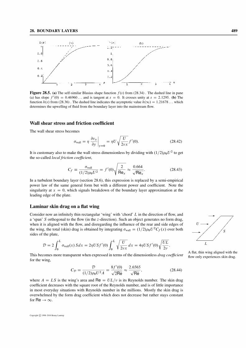
Figure 28.5. (a) The self-similar Blasius shape function f .s/ from (28.34) . The dashed line in pane(a) has slope f 0.0/ D 0:46960 : : : and is tangent at s D 0. It crosses unity at s D 2:1295. (b) Thefunction h.s/ from (28.36) . The dashed line indicates the asymptotic value h.1/ D 1:21678 : : : whichdetermines the upwelling of fluid from the boundary layer into the mainstream flow.
Wall shear stress and friction coefficientThe wall shear stress becomes
�wall D �@vx
@y
ˇyD0
D �U
rU
2�xf 0.0/: (28.42)
It is customary also to make the wall stress dimensionless by dividing with .1=2/�0U 2 to getthe so-called local friction coefficient,
Cf ��wall
.1=2/�0U 2D f 0.0/
s2
Rex�
0:664p
Rex: (28.43)
In a turbulent boundary layer (section 28.6), this expression is replaced by a semi-empiricalpower law of the same general form but with a different power and coefficient. Note thesingularity at x D 0, which signals breakdown of the boundary layer approximation at theleading edge of the plate.
Laminar skin drag on a flat wing
%%%%%%%�
������
L
S-
-
-
U
A flat, thin wing aligned with theflow only experiences skin drag.
Consider now an infinitely thin rectangular ‘wing’ with ‘chord’ L in the direction of flow, anda ‘span’ S orthogonal to the flow (in the z-direction). Such an object generates no form drag,when it is aligned with the flow, and disregarding the influence of the rear and side edges ofthe wing, the total (skin) drag is obtained by integrating �wall D .1=2/�0U
2Cf .x/ over bothsides of the plate,
D D 2Z L
0
�wall.x/ Sdx D 2�USf0.0/
Z L
0
rU
2�xdx D 4�USf 0.0/
rUL
2�:
This becomes more transparent when expressed in terms of the dimensionless drag coefficientfor the wing,
CD DD
.1=2/�0U 2AD8f 0.0/p2Re
�2:6565p
Re; (28.44)
where A D LS is the wing’s area and Re D UL=� is its Reynolds number. The skin dragcoefficient decreases with the square root of the Reynolds number, and is of little importancein most everyday situations with Reynolds number in the millions. Mostly the skin drag isoverwhelmed by the form drag coefficient which does not decrease but rather stays constantfor Re!1.
Copyright c 1998–2010 Benny Lautrup
490 PHYSICS OF CONTINUOUS MATTER
Example 28.4 [Weather vane]: A little rectangular metal weather vane with sides L D30 cm and S D 20 cm in a U D 10 m s�1 wind has Re D UL=� � 2� 105, well below the onsetof turbulence. The drag coefficient becomes CD � 6� 10�3, and the total skin drag D � 0:02 N,when the vane is aligned with the wind. This drag corresponds to a weight of merely 2 g, whereasthe form drag and the other aerodynamic forces that align the vane are much stronger. One shouldcertainly not dimension the support of the vane on the basis of the laminar skin drag!
28.6 Turbulent boundary layer in uniform flow
Sufficiently far downstream from the leading edge, the Reynolds number, Rex D Ux=�,will eventually grow so large that the boundary layer becomes turbulent. Empirically, thetransition happens for 5 � 105 . Rex . 3 � 106, depending on the circumstances, forexample the uniformity of the mainstream flow and the roughness of the plate surface. Weshall in the following discussion take Rex D 5 � 105 as the nominal transition point.
Sketch of the thickness of theboundary layer from the leadingedge through the transition re-gion. At the transition (dashedline), the turbulent layer growsrapidly whereas the viscous sub-layer only grows slowly.
The line of transition across the plate is not a straight line parallel with the z-axis, butrather an irregular, time-dependent, jagged, even fractal interface between the laminar andturbulent regions. This is also the case for the extended, nearly ‘horizontal’ interface betweenthe turbulent boundary layer and the fluid at large. Such intermittent and fractal behaviour iscommon to the onset of turbulence in all systems.
Friction coefficient
In a turbulent boundary layer, the true velocity field v fluctuates in all directions and in timearound some mean value. Even very close to the wall, there will be notable fluctuations. Theno-slip condition nevertheless has to be fulfilled and a thin sublayer dominated by viscousstresses must exist close to the wall. In this viscous sublayer the average velocity Nvx riseslinearly from the surface with a slope, @ Nvx=@yjyD0 D N�wall=� that can be determined fromdrag measurements.
A decent semi-empirical expression for the friction coefficient of a turbulent boundarylayer was already given by Prandtl (see for example [White 1999, White 1991] for details)
Cf �N�wall
1=2�0U 2�0:027
Re1=7x: (28.45)
The turbulent friction coefficient thus decreases much slower than the corresponding laminarfriction coefficient (28.43) . The two expressions cross each other at Rex � 7800which is farbelow the transition to turbulence, implying a jump from Cf � 9:4�10
�4 toCf � 4:1�10�3
at Rex � 5 � 105. Turbulent boundary layers thus cause much more skin drag than laminarboundary layers (by a factor of more than four at the nominal transition point).
In figure 28.6 the friction coefficient is plotted across the laminar and turbulent regimes.The transition from laminar to turbulent is in reality not nearly as sharp as shown here, partlybecause of the average over the jagged transition line. Eventually, for sufficiently large Rex ,the roughness of the plate surface makes the friction coefficient nearly independent of viscos-ity and thus of Rex .
Drag on a flat wing
Let us again consider a finite ‘wing’ of size A D L � S . For sufficiently large Reynoldsnumber Re D UL=�, the boundary layer will always become turbulent some distance down-stream from the the leading edge, and the drag will in general be dominated by the turbulentboundary layer’s larger friction coefficient. Assuming a fully turbulent boundary layer, the
Copyright c 1998–2010 Benny Lautrup
28. BOUNDARY LAYERS 491
Figure 28.6. Schematic plot of the local friction coefficient Cf D N�wall.x/=.1=2/�0U2 across the
laminar and turbulent regions as a function of the downstream Reynolds number Rex D Ux=�. Thetransitions at the nominal points Rex D 5 � 105 and at Rex D 109 are in reality softer than shownhere. The position of the second transition and the terminal value of Cf depend on the roughness of theplate surface (see [White 1999] for details).
dimensionless turbulent drag coefficient becomes (including both sides of the plate)
CD D2
1=2�0U 2A
Z L
0
N�wall.x/ Sdx D0:063
Re1=7: (28.46)
If the leading laminar boundary layer cannot be disregarded, this expression is somewhatmodified.
Example 28.5 [Flag blowing in the wind]: A A D 2 � 2 m2 flag in a U D 10 m s�1 windhas a Reynolds number of Re � 1:3�106, well inside the turbulent region. The laminar skin dragcoefficient is CD � 2:3 � 10�3 whereas the turbulent skin drag coefficient is CD � 8:4 � 10�3.The turbulent skin drag is only D � 1:68 N which seems much too small to keep the flag straight.But flags tend to flap irregularly in the wind, thereby adding a much larger average form drag tothe total drag, and giving them even in a moderate wind the nearly straight form that we admire somuch.
Local drag and momentum balance
x1 x2
The drag on the plate between x1and x2 must equal the rate of lossof momentum from the fluid be-tween the dashed lines.
Momentum balance guarantees that the drag on any section of the plate, say for x1 < x < x2,must equal the rate of momentum loss from the slice of fluid above this interval, independentof whether the fluid is laminar or turbulent. Formally, we may use the Prandtl equations toderive such a relation for an infinitesimal slice of the boundary layer, as was first done by vonKarman in 1921.
For constant slip-flow it follows trivially from (28.28) and (28.33) that
Integrating over all y and using the boundary conditions, we see that the second term on the
Copyright c 1998–2010 Benny Lautrup
492 PHYSICS OF CONTINUOUS MATTER
Figure 28.7. Schematic plot of the dimensionless ‘true’ thickness, represented by Reı D Uı=�, as afunction of downstream distance x, represented by Rex D Ux=�. Also shown is the thickness of theviscous sublayer ı� . The momentum thickness ımom is obtained from the refined expression (28.54)and is everywhere roughly a factor 10 smaller than the ‘true’ thickness ı. The real transition at thenominal value, Rex D 5 � 105, is even softer than shown here. The transition from smooth to roughplate at Re D 109 is barely visible.
right-hand side does not contribute, and we obtain
�@vx
@y
ˇyD0
Dd
dx
Z 10
.U � vx/vx dy: (28.48)
The quantity on the left-hand side is simply �wall=�0, and the integral on the right-hand sideis the flux of lost momentum. In section 28.8 we shall make a more systematic study of suchrelations.
The turbulent velocity profile isapproximately a power Nvx � y
with � 1=7. The vertical tan-gent at y D 0 is unphysical,because it implies infinite wallstress. A finite wall stress is pro-vided by a thin viscous sublayer.
Empirically, the flat-plate turbulent boundary layer profile outside the thin viscous sublayer isdecently described by the simple model (due to Prandtl [White 1991]),
vx
UD
�yı
�1=7; .0 . y < ı/: (28.49)
Ignoring the sublayer which cannot contribute much to the integral, we obtainZ ı
0
.U � vx/vx dy D7
72U 2ı: (28.50)
Although the thickness ı is not known at this stage, we may use the von Karman relation(28.48) to relate it to the friction coefficient, for which we have the semi-empirical expression(28.45) . In this way we obtain an ordinary differential equation for the thickness,
dı
dxD36
7Cf : (28.51)
Copyright c 1998–2010 Benny Lautrup
28. BOUNDARY LAYERS 493
In a fully turbulent boundary layer, we may integrate this equation using (28.45) with theinitial value ı D 0 at x D 0, to get
ı D36
7
Z x
0
Cf dx � 0:16�
URe6=7x : (28.52)
Expressing the thickness in dimensionless form by means of the local Reynolds number, wefinally have
Reı �Uı
�D 0:16Re6=7x : (28.53)
The jump in the local Reynolds number at the nominal transition point x D x0 where Rex0 D5 � 105, is only apparent. A more precise expression for the local Reynolds number may beobtained by using the Blasius result for 0 � x � x0, and integrating the turbulent expressiononly for x > x0,
Reı D
8<:5p
Rex x < x0
5p
Rex0 C 0:16�Re6=7x � Re6=7x0
�x > x0:
(28.54)
By construction, this expression is continuous across the nominal transition point (see fig-ure 28.7).
The ‘true’ thickness ı� of the vis-cous sublayer is obtained fromthe intercept between Prandtl’spower profile (28.49) and the lin-early rising velocity in the sub-layer. The kink at y D ı�is unphysical, because it givesrise to a small jump in shearstress that violates Newton’s thirdlaw (slightly). The real transi-tion from viscous sublayer to tur-bulent main layer is softer thanshown here.
It is also possible to get an estimate of the thickness ı� of the viscous sublayer from theintercept between the linearly rising field, vx D y N�wall=�, in the sublayer and the power law(28.49) . Demanding continuity at y D ı� , we get
N�wall
�ı� D U
�ı�
ı
�1=7:
Solving this equation for ı� and inserting �wall from (28.45) and ı from (28.53) we obtainthe remarkable expression,
Uı�
�D 206Re1=42x : (28.55)
At the nominal transition point Rex D 5 � 105, this becomes 282, which grows to 337 atRex D 109. The sublayer thickness is also plotted in figure 28.7 and its variation with Rexis barely perceptible.
It is now also possible to calculate what fraction of the terminal velocity the fluid hasachieved at the ‘edge’ of the sublayer,
vxjyDı�U
D 2:8Re�5=42x : (28.56)
At the nominal transition point it is 0.59 and falls by roughly a factor 2 to 0.24 at Rex D 109.
Copyright c 1998–2010 Benny Lautrup
494 PHYSICS OF CONTINUOUS MATTER
* 28.7 Self-similar boundary layersIn the two preceding sections we have only discussed the case of constant slip-flow, but nowwe turn to the study of slip-flows that vary with x. In this section we shall focus on thegeneralization of the self-similar laminar Blasius solution to non-constant flat-plate slip-flowU.x/. The assumption of self-similarity has before allowed us to convert the partial differen-tial equations of fluid mechanics into ordinary differential equations. We shall now see thatself-similarity implies that the Prandtl equations essentially only permit power law slip-flowsof the form U � xm. The class of such slip-flows is on the other hand sufficiently general toillustrate what happens when a slip-flow accelerates (m > 0) or decelerates (m < 0), althoughit cannot handle the separation phenomenon.
The Falkner–Skan equationA self-similar flow is defined to be of the form,
vx D U.x/f .s/; s Dy
ı.x/; (28.57)
where f .s/ is a dimensionless function of the dimensionless variable. The velocity scale isset by U.x/ and the scale of the boundary layer thickness by ı.x/. As for the Blasius layer wechoose the boundary conditions to be f .0/ D 0 and f .1/ D 1. In the following we suppressthe x-dependence wherever possible.
It follows immediately from the equation of continuity (28.29) that
vy D �@
@x.Uıg/; (28.58)
where g.s/ is again given by (28.35) . Substituting vx and vy into the Prandl equation (28.33)we obtain after a little algebra the coupled ordinary differential equations,
f 00 C ˛gf 0 C ˇ.1 � f 2/ D 0; g0 D f; (28.59)
where a prime indicates the derivative with respect to s. Using a dot to denote the derivativeafter x, the purely numerical coefficients become,
˛ Dı PıU C ı2 PU
�; ˇ D
ı2 PU
�; (28.60)
and may by construction be x-dependent. The crucial point is now that since f .s/ and g.s/only depend on s, it follows from the differential equation (28.59) that both ˛ and ˇ must infact be independent of x.
The definitions (28.60) may thus be viewed as two coupled ordinary differential equationsfor ı and U with constant values of ˛ and ˇ. To solve them we first note that they implyd.ı2U/=dx D .2˛ � ˇ/�. For ˛ > 0 we may without loss of generality rescale ı such thatwe get ˛ D 1. Integrating we now obtain ı2U D .2 � ˇ/�x where for ˇ ¤ 2 we choose theorigin of x such that integration constant vanishes. Inserting this into the second equation in(28.60) , it follows that ˇ D .2 � ˇ/x PU=U , implying that U � xm with m D ˇ=.2 � ˇ/.Putting it all together, the allowed class is given by,
U.x/ D Axm; ı.x/ D
s2�x
.1Cm/U.x/; (28.61)
where A > 0 is a constant. For m D 0 this reduces to the Blasius case with ı Dp2�x=U .
Copyright c 1998–2010 Benny Lautrup
28. BOUNDARY LAYERS 495
Figure 28.8. Self-similar Falkner–Skan velocity profiles f .s/ for select values of mc < m < 1
where mc D �0:0904286. The Blasius profile is obtained for m D 0. Note that there are two solutionsfor each value of m in the interval mc < m < 0, one of which has reversed flow close to the wall. Thecritical profile with m D mc is shown dashed.
The resulting nonlinear third-order differential equation,
g000 C gg00 C ˇ.1 � g02/ D 0; (28.62)
with ˇ D 2m=.1Cm/ was introduced in 1931 by Falkner and Skan2, and the one-parameterfamily of solutions has since been extensively studied [Schlichting and Gersten 2000, Sobey 2000].A selection of profiles are shown in figure 28.8 for a few values of m. We leave it as an exer-cise to discuss the other families of solutions with ˛ � 0 or ˇ D 2.
UpflowA non-constant inviscid slip-flow vx D U.x/ generates by itself (and mass conservation) anupflow vy D �y PU.x/. The part of the upflow due to the presence of a boundary layer isconsequently vy C y PU , which may be written in the form
vy C y PU.x/ D�
ıh.s/; (28.63)
h.s/ D sf .s/ � g.s/C ˇs.1 � f .s//: (28.64)
This reduces to the Blasius result (28.36) for ˇ D 0. Since for s ! 1 we expect thatf .s/ ! 1 with an exponential tail, this function converges for s ! 1 to a finite value,h.1/ D lims!1.s � g.s//.
Numeric method and resultsNumeric integration of the Falkner–Skan equation is reasonably straightforward using a ‘bal-listic’ method of integration. The integration process is initiated with g.0/ D f .0/ D 0 and
2V. M. Falkner and S.W.Skan, Some approximate solutions of the boundary layer equations, Phil. Mag. 12,(1931) 865.
Copyright c 1998–2010 Benny Lautrup
496 PHYSICS OF CONTINUOUS MATTER
Figure 28.9. (a) The wall slope f 0.0/ as a function of m in the interval �0:1 � m � 0:2. It is double-valued for negative m, and the negative solution (dotted) joins continuously with vertical tangent to thepositive solution at the critical pointmc D �0:0904286 : : :. (b) The limiting upflow h.1/ as a functionof m. It is also double-valued for negative m and takes the value h.1/ D 2:35885 : : : for m D mc .
f 0.0/ D �, and a search is made for the value of the slope � that yields f .1/ D 1. In thesame way as there are two elevation angles that may be used to hit a target with a cannon ball,there may be more than one solution to the Falkner–Skan equation for certain values of m.
In figure 28.8 the velocity profile is shown for a selection of m-values and in figure 28.9the wall slope f 0.0/ and asymptotic upflow h.1/ are plotted as a function ofm in the interval�0:1 < m < 0:2. The most conspicuous feature of the figures is the existence of two solutionsin the intervalmc < m < 0 wheremc D �0:0904286 : : :. One solution has positive slope andthe other negative, indicating backflow in the boundary layer. The slope vanishes at the criticalpoint m D mc , where the positive solution joins with the negative with vertical tangent.
Accelerating and decelerating slip-flow
In the region 0 < m < 1 the slip-velocity increases downstream. The solutions are uniqueand all resemble the Blasius solutions, except that the thickness scale
ı.x/ � x.1�m/=2 (28.65)
grows slower thanpx. For m > 1 the layer is even suppressed by the accelerating flow and
gets thinner with x.For �1 < m < 0 the slip-flow decelerates and the thickness grows faster than
px. There
are, as mentioned, precisely two solutions in the interval mc < m < 0. Just below thecritical point, in the interval �1=3 < m < mc , there are no solutions at all, but for any min the interval �1 < m < �1=3 there appears to be from one to three distinct solutionswith different values of the slope [Sobey 2000]. These solutions oscillate and overshoot whileconverging upon f .1/ D 1. They are of no interest in the context of flat plate boundarylayers.
Separation?
Self-similar flows can strictly speaking not be used to model separation, because the velocityprofile by construction has the same general shape for all x. If we let m slide down towardsthe critical valuemc , it nevertheless looks very much as if separation does take place (all overthe x-axis at the same time). At the critical point, where the positive solution joins with thebackflowing negative solution, there is a singularity with infinite slope derivative f 00.mc/.Such singularities are generic for the Prantdl equations (see section 28.9).
0, the wall curvature is negative,whereas in decelerating flow thecurvature is positive. The dashedcurve sketches the velocity pro-file for vanishing wall curvature.
A varying slip-flow U.x/ will strongly influence the flow in the boundary layer. Acceleratingflow with dU=dx > 0 tends to suppress the boundary layer, so that its downstream thicknessgrows slower than the
px of the Blasius layer. Sufficiently strong acceleration may even
make the boundary layer become thinner downstream. Conversely, if the slip-flow decelerates,dU=dx < 0, the thickness will grow faster than
px, and sufficiently strong deceleration may
lift the boundary layer off the plate and make it wander into the mainstream as a separatedboundary layer.
In this section we shall establish some relations that are valid for any exact solution toPrandtl’s equations. These relations will be useful for the discussion of the separation phe-nomenon to be taken up in section 28.9. Although we shall always think of a flat plateboundary layer, the following discussion is also valid for slowly curving walls, such as themuch-studied flow around a cylinder.
Exact wall derivatives
At the wall, y D 0, we know that both vx and vy must vanish, and that the derivative of thevelocity at the wall,
� D@vx
@y
ˇyD0
(28.66)
is in general non-vanishing, except at a separation point, where it has to vanish. The wallvorticity is !z D ��.
Setting y D 0 in the Prandtl equation (28.33) we immediately get the double derivative,also called the wall curvature,
�@2vx
@y2
ˇyD0
D �UdU
dx: (28.67)
Its direct relation to the slip-flow opens up a qualitative discussion of the shape of the velocityprofile. If the slip-flow accelerates (dU=dx > 0), the wall curvature will be negative andfavor the approach of the velocity towards its terminal value, U . Conversely, if the slip-velocity decreases (dU=dx < 0), the wall curvature will be positive and adversely affect theapproach to terminal velocity. This forces an inflection point into the velocity profile andraises the need for including higher derivatives to secure the turn-over towards the asymptoticslip-flow. For constant slip-flow, i.e. the Blasius case, we have dU=dx D 0, and the wallcurvature vanishes.
The higher order wall derivatives may be calculated by differentiating the Prandtl equationrepeatedly with respect to y. Differentiating once, we find
�@3vx
@y3
ˇyD0
D 0; (28.68)
and once more
�@4vx
@y4
ˇyD0
D �d�
dx: (28.69)
Clearly, this process can be continued indefinitely to obtain all wall derivatives of vx depend-ing only on U , � and their derivatives.
Copyright c 1998–2010 Benny Lautrup
498 PHYSICS OF CONTINUOUS MATTER
Exact integral relationsWe have already derived a relation (28.48) from momentum balance in uniform flow. Forgeneral varying slip-flow we first rewrite the Prandtl equation (28.33) in the form,
��@2vx
@y2D .U � vx/
dU
dxC@Œvx.U � vx/�
@xC@Œvy.U � vx/�
@y: (28.70)
Integrating this equation over y from 0 to 1, and using the boundary values vy ! 0 fory ! 0 and U � vx ! 0 for y !1, we obtain the general von Karman relation
�@vx
@y
ˇyD0
DdU
dx
Z 10
.U � vx/ dy Cd
dx
Z 10
.U � vx/vx dy: (28.71)
It states that the drag on any infinitesimal interval of the plate equals the rate of momentumloss from the slice of fluid above the interval.
We may similarly derive a relation expressing kinetic energy balance by multiplying thePrandtl equation with vx , and rewriting it in the form,
�
�@vx
@y
�2D1
2�@2.v2x/
@y2C1
2
@..U 2 � v2x/vx/
@xC1
2
@.vy.U2 � v2x//
@y: (28.72)
Integrating this over all y and using the boundary conditions, we get
�
Z 10
�@vx
@y
�2dy D
1
2
d
dx
Z 10
.U 2 � v2x/vx dy: (28.73)
This relation states that the rate of heat dissipation in any infinitesimal slice equals the rate ofloss of kinetic energy from the fluid. It is also possible to derive further relations for angularmomentum balance and thermal energy balance [White 1991, Schlichting and Gersten 2000].
The integrands in the momentum and energy balance equations, (28.71) and (28.73) , maybe interpreted physically in terms of flow properties. The expression U �vx is the volume fluxof fluid displaced by the plate, the expression �0.U � vx/vx is the flux of ‘lost momentum’caused by the presence of the plate, 1=2�0.U 2�v2x/vx is the flux of ‘lost kinetic energy’, and�.@vx=@y/
Definition of displacement thick-ness from the integral of the fluxof volume loss, U � vx .
It is convenient to introduce dynamic length scales (or thicknesses) related to each of thesequantities (and the wall stress),
1
ı wallD
1
U
@vx
@y
ˇyD0
; (28.74a)
ıdisp D1
U
Z 10
.U � vx/ dy; (28.74b)
ımom D1
U 2
Z 10
.U � vx/vx dy; (28.74c)
ıener D1
U 3
Z 10
.U 2 � v2x/vx dy; (28.74d)
1
ı heatD
1
U 2
Z 10
�@vx
@y
�2dy: (28.74e)
Copyright c 1998–2010 Benny Lautrup
28. BOUNDARY LAYERS 499
Figure 28.10. Laminar boundary layer separation from a sphere at Re D 15 000. Note how theboundary layer separates at the forward facing half of the sphere. ONERA photograph, H. Werle Rech.Aerospace 198-5 (1980) 35–49.
In terms of these thicknesses, the momentum and energy balance equations now take thecompact and quite useful forms,
�U
ıwallD U
dU
dxıdisp C
d�U 2ımom
�dx
; (28.75a)
�U 2
ıheatD1
2
d.U 3ıener/
dx(28.75b)
We emphasize that these relations, like the wall derivatives (28.67) –(28.69) , are fulfilled forany exact solution to the boundary layer equations.
The self-similarity thus guarantees that the ratios between any thicknesses are pure numbersindependent of x. The integral relations (28.75) simplify in this case to,
2ıwallımom D ıheatıener D 2ı2: (28.77)
These relations are of course fulfilled for the numeric values above.
Copyright c 1998–2010 Benny Lautrup
500 PHYSICS OF CONTINUOUS MATTER
28.9 Laminar boundary layer separationWhen a separating boundary layer takes off into a decelerating mainstream, the character ofthe mainstream flow is profoundly changed, thereby actually invalidating the Prandtl approx-imation. Careful analysis has revealed that this is a generic problem, to which the boundarylayer equations respond by developing an unphysical singularity at the point of separation.This so-called Goldstein singularity [Sobey 2000] prevents us in general from using bound-ary layer theory to connect the regions before and after separation.
Although Prandtl’s boundary layer theory for this reason is useless for separation prob-lems, the existence of a singularity is nevertheless believed to be an indicator of boundarylayer separation in the general vicinity of the point where the singularity occurs. During thetwentieth century the problem of predicting the singular separation point for boundary layersaround variously shaped objects has been of great importance to fluid mechanics, for funda-mental as well as technological reasons. It has proven to be a challenging problem, to say theleast [Schlichting and Gersten 2000, Sobey 2000]. A number of approximative schemes havebeen proposed and tried out, and with suitable empirical input, they compare reasonably wellwith analytic or numeric calculations [White 1991].
The Goldstein singularity is unavoidable as long as we persist in the belief that we canemploy Prandtl’s equations and also specify the slip-flow velocity as we wish. The price topay for avoiding the singularity is that the Prandtl equations must be replaced by the Navier–Stokes equations and that the mainstream flow cannot be fully specified in advance, but has tobe allowed to be influenced by what happens deep inside the boundary layer. Since separationoriginates in the innermost viscous ‘deck’ of the boundary layer, viscosity thus takes a decisivepart in selecting the presumed inviscid flow at large, again emphasizing that inviscid flowsolutions are not unique, and that inviscid flow is indeed an ideal.
Sydney Goldstein (1903–89).British mathematical physicist.Worked on numerical solutions tothe steady-flow laminar boundarylayer equations.
Schematic picture of how sepa-ration is thought to take placein a decelerating flow. Themainstream flow is profoundlychanged by the separation bothupstream and downstream fromthe separation point.
In the last half of the twentieth century, it has been conclusively demonstrated throughtheoretical analysis and numerical simulation that the Navier–Stokes equations do not leadto any boundary layer singularities and do in fact smoothly connect the regions before andafter separation. The most successful method is in fact a natural extension of Prandtl’s idea ofdividing the flow into two ‘decks’, a viscous transition layer and an inviscid slip-flow layer,that in the end are ‘stitched together’ to form a complete boundary layer. In the ‘triple deck’approach the transition layer is further subdivided into a near-wall viscous sublayer and asecond viscous layer interpolating between the sublayer and the slip-flow. Unfortunately,there does not seem to be any simple way of presenting this modern ‘interactive’ boundarylayer theory [Schlichting and Gersten 2000, Sobey 2000, Sychev et al. 1998].
In this section we shall first justify that the Goldstein singularity exists, and make a prim-itive attempt to determine its position in a number of cases where the exact position is known(table 28.1). In the remainder of the section we shall see that it is possible to predict theposition of the singularity to an accuracy better than 1% from momentum and energy bal-ance alone without any empirical input. A simplified version of this model yields an accuracybetter than 3%.
The wall-anchored modelThe simplest model of boundary layer flow is obtained by approximating the velocity profilewith a fourth-order polynomial in y constructed from the exact wall derivatives (page 497)
vx D �y �U PU
2�y2 C
� P�
24�y4; (28.78)
where a dot is used to denote differentiation with respect to x. Evidently, this expression isexact for y ! 0, but for y !1 where all three terms diverge, there is of course a problem.In decelerating slip-flow ( PU < 0), the second-order term is always positive, and the fourth-order term is always negative just upstream from the separation point, because the slope � is
Copyright c 1998–2010 Benny Lautrup
28. BOUNDARY LAYERS 501
positive and decreasing towards zero at separation. After an initial rise governed by the first-and second-order terms, the fourth-order term must eventually pull down the profile to minusinfinity, unless we ‘catch’ it at the top.
Wall-anchored fourth-order poly-nomial joins continuously withvx D U at its maximum y D ı.The continuation beyond ı dropsto �1 in a decelerating slip-flowand is unphysical.
We ‘catch’ the profile by requiring the velocity to join smoothly at maximum with thegiven slip-flow U.x/, i.e. vx D U.x/ and @vx=@y D 0 at y D ı, resulting in the conditions,
� ı �U PU
2�ı2 C
� P�
24�ı4 D U; (28.79a)
� �U PU
�ı C
� P�
6�ı3 D 0: (28.79b)
Eliminating � P� between these equations we obtain an algebraic relation between � and ı,
� D4U
3ı
1C
PUı2
4�
!: (28.80)
This shows that there is in fact only one free parameter in the problem, say ı, satisfying afirst-order differential equation (see problem 28.6). It also follows from this relation thatsince � D 0 at a separation point the thickness ıc D ı.xc/ will be finite here,
ıc D 2
r��
PUc; (28.81)
where PUc D PU.xc/ is the ‘deceleration’ at the separation point ( PUc < 0).From the second condition (28.79b) the behaviour of � P� can be now determined in the
vicinity of the separation point, where
2� P� � �3Uc PU
2c
�: (28.82)
Integrating over x using � D 0 for x D xc we arrive at,
� � �pxc � x; � D � PUc
r3Uc
�; (28.83)
which clearly demonstrates the existence of the Goldstein singularity.Near the wall just upstream from the separation point, the velocity profile becomes,
vx � �y � � ypxc � x; (28.84)
and from mass conservation (28.29) we determine the corresponding upflow
vy � �1
2
d�
dxy2 �
�
4
y2pxc � x
: (28.85)
Evidently, the upflow diverges for all y at the separation point. Apart from being totallyunphysical, this shows that it is not possible to solve the separation problem within the Prandtlapproximation itself, because one of the conditions for this approximation,
ˇvyˇ� jvxj, fails
miserably near the separation point.The model is analysed further in problem 28.6. The separation points obtained from nu-
meric integration of this model are listed in the third column (marked ‘wall’) in table 28.1 fornine decelerating slip-flows. They agree rather poorly with the exact results (second column),overshooting by up to 50%. The poor performance of the model must be ascribed to the muchtoo solid anchoring of the boundary layer to the wall, which tends to generate errors in theshape of the velocity profile in the bulk of the boundary layer.
Copyright c 1998–2010 Benny Lautrup
502 PHYSICS OF CONTINUOUS MATTER
Table 28.1. Table of decelerating slip-flows and the positions of their Goldstein singularities (‘sep-aration points’) calculated in various models discussed in the text. The exact values xc in the secondcolumn are taken from [White 1991]. The separation points determined by the wall-anchored fourth-order polynomial (28.78) are listed in the third column, and have typical errors of 40%. The fourthcolumn is obtained by Pohlhausen’s method (28.111) . It has errors less than 25% and is in all casesbetter than the wall-anchored approximation. In the fifth column the separation points are determinedfrom both momentum and energy balance (28.75) with typical errors smaller than 1%. Finally, in thelast column, the separation points are derived from the simple approximation (28.97) with the typicalerror being less than 3%.
U.x/ xc wall wallCmom momCener approximation
1. 1 � x 0.120 0.176 0.157 0.121 0.1232.p1 � x 0.218 0.314 0.277 0.219 0.221
The fourth-order polynomialjoins smoothly with vx D U
with a horizontal inflection pointat y D ı. The continuation be-yond y D ı which diverges toC1 for � < 3 is not used.
The wall-anchored approximation (28.78) suffers from an unnatural jump in the curvature@2vx=@y
2 at the edge of the boundary layer at y D ı. A smoother fourth-order polynomialwas introduced by Pohlhausen in 1921, in which the coefficients are fixed by demanding thefield to approach vx D U at y D ı with vanishing first- and second-order derivatives,
vx
UD �
y
ıC 3.2 � �/
�yı
�2� .8 � 3�/
�yı
�3C .3 � �/
�yı
�4: (28.86)
It contains two unknown functions: the dimensionless slope at the wall �.x/ and the layerthickness ı.x/. One may readily verify that this is indeed O
�.y � ı/3
�for y ! ı.
Note that for � < 2, the second- and fourth-order terms are always positive. It is thenegative third-order term, which secures the smooth turn-over towards the slip-flow at y D ı.A selection of this family of profiles is shown in figure 28.11. The profiles are well definedfor all �, both before the separation point (� > 0) and after (� < 0). After separationthey exhibit backflow, as one would expect, but the Goldstein singularity prevents us fromconnecting these two regions of solutions.
Pohlhausen solved the model by imposing the wall-curvature condition (28.67) togetherwith the von Karman relation (28.75a) . The details are given in problem 28.7, and the separa-tion point predictions are tabulated in the fourth column (marked ‘wall+mom’) of table 28.1.The agreement is still rather poor with typical errors of 25%.
Momentum and energy balanceThe nearly self-similar form of the Pohlhausen family (28.86) implies that all thicknesses arepolynomials in � scaled by ı. The wall, displacement and momentum thicknesses become
ı
ıwallD �;
ıdisp
ıD2
5
�1 �
�
8
�;
ımom
ıD
4
35
�1C
�
12�5�2
144
�; (28.87)
Copyright c 1998–2010 Benny Lautrup
28. BOUNDARY LAYERS 503
Figure 28.11. Profiles of the Pohlhausen family for integer values of � from �5 to C5. The dashedcurve is the profile at separation, corresponding to � D 0, and the profiles with � < 0 have backflow.
and the energy and heat thicknesses,
ıener
ıD
876
5005
�1C
�
12�253�2
10512�7�3
3504
�;
ı
ıheatD48
35
�1 �
�
12C�2
16
�: (28.88)
Inserting these into the integral relations (28.75) , one arrives at two rather horrible coupledfirst-order differential equations for ı and �. These differential equations are derived in prob-lem 28.8 and solved numerically with the results shown in the column marked ‘momCener’of table 28.1. They agree with the exact singularities to better than 1% in nearly all cases,demonstrating that together momentum and energy balance do predict the position of theGoldstein singularity with acceptable precision.
Approximative solutionWe now turn to the question of whether it is possible to simplify the model and still retaina reasonable predictive ability. The approximation is based on the observation that the di-mensionless ratios ımom=ıener and ıener=ıheat are nearly constant because the terms linear in �cancel in the ratios (see also figure 28.12).
Multiplying the energy relation (28.75b) with 4U 3ıener, we may rewrite it as
d.U 6ı2ener/
dxD 4�U 5
ıener
ıheat: (28.89)
Approximating the ratio by a constant, we may integrate the equation to get,
U 6ı2ener � 4�ıener
ıheat
Z x
0
U.x/5 dx: (28.90)
The integral defines a slip-flow length scale
L.x/ D1
U.x/5
Z x
0
U.x/5 dx; (28.91)
and the energy relation may now be expressed as
ıheatıener D 4�L.x/
U.x/; (28.92)
Copyright c 1998–2010 Benny Lautrup
504 PHYSICS OF CONTINUOUS MATTER
Figure 28.12. Nearly constant thickness ratios in the Pohlhausen family. (a) The ratio ımom=ıenervaries by about 1.3% around its mean value between � D 0 and � D 2. (b) The ratio ıener=ıheat variesby about 6.6% around its mean value in the same interval.
which is of the same general form as the Blasius result (28.77) , corresponding to L.x/ D x.The momentum equation (28.75a) is analogously multiplied with 2U 4ımom, and rewritten
in the form,
2�U 5ımom
ıwallD 2U 5 PU
�ıdisp
ımom� 1
�ı2mom C
d.U 6ı2mom/
dx: (28.93)
Writing ı2mom D ı2ener.ı2mom=ı
2ener/ and approximating the ratio ı2mom=ı
2ener by a constant, we
may use (28.89) to get the following algebraic relation between the various thicknesses
2�ımom
ıwallD 2 PU
�ıdisp
ımom� 1
�ı2mom C 4�
ı2mom
ıenerıheat: (28.94)
Rewriting this expression by means of (28.92) it becomes a dimensionless relation,
PUL
UDıenerıheat � 2ımomıwall
4ıwall.ıdisp � ımom/� R.�/: (28.95)
Since the left-hand side depends only on the given velocity U.x/, and the right-hand side isa known rational function of �.x/ in the Pohlhausen model (see problem 28.9), this equationmay be solved for �.x/. Having obtained �.x/ one may then search for a separation pointwhere �.x/ D 0. For the Blasius layer where there is no separation point, the left-hand sidevanishes and we obtain instead from the right-hand side ıheatıener D 2ıwallımom, a relationwhich we have already derived in (28.77) .
At the separation point � ! 0 the wall thickness diverges, ıwall ! 1, while the otherthicknesses remain finite, such that
PUL
U! �
1
2
ımom
ıdisp � ımom
ˇ�D0
D �1
5; (28.96)
where on the right-hand side we have used the Pohlhausen family value ıdisp=ımom D 7=2 for� D 0. Inserting (28.92) we obtain an equation that the separation point x D xc must satisfy,
PU.xc/
U.xc/6
Z xc
0
U.x/5 dx D �1
5: (28.97)
Solving this equation for the usual test cases we find the results shown in the last column oftable 28.1. The errors are typically less than 3% which is as good as the semi-empirical meth-ods [White 1991]. The model also predicts �.x/ via (28.95) and thus all the thickness ratios(28.87) and (28.88) . The absolute thickness scale ı.x/ is finally obtained from (28.92) .
Sketch of the much-studied sepa-ration flow around a cylinder (ofwhich only half is shown here).The separating streamline is dot-ted.
Some of the more interesting slip-flows first accelerate and then decelerate. Among them thenotorious cylinder in a uniform cross-wind, which has been the favourite target for boundarylayer research for nearly a hundred years. The cylinder presents two difficulties, as does infact every realistic separation problem. The first is the question of what is the correct slip-flow. Since separation interacts with the mainstream flow, this is not so simple. The second isthe technical question of calculating a precise value for the separation point in a slip-flow thatmay not be purely decelerating.
If the external flow around the cylinder is taken to be the potential flow, the slip-flow isgiven by (13.37b), i.e. U.x/ D 2U0 sin x where U0 is the strength of the uniform cross-windand x is the angle of observation (the upwind direction corresponds to x D 0). The approxi-mative equation (28.97) immediately yields xc D 1:800 D 103 ı. The exact separation pointfor this slip-flow (obtained by numerical calculation) is known to be xc D 1:823 � 104 ı (see[White 1991]), so in this case the approximation works to a precision only slightly worse than1%.
The real flow around the cylinder is, however, not potential flow because of the vorticityinduced into the main flow by the boundary layer, especially in the separation region andbeyond. Hiemenz (1911) determined experimentally that the slip-flow at a Reynolds numberRe D U0a=� D 9500 was well described by the odd polynomial [White 1991, p. 272],
U D U0.1:814x � 0:271x3� 0:0471x5/: (28.98)
Now the approximative equation (28.97) predicts separation at xc D 1:372 D 78:6 ı which isonly about 2% away from the value xc D 80:5 ı measured by Himenz. Even if agreement isobtained, this is not very impressive, because the slip-flow itself has not been calculated fromfirst principles. Most of the information about the separation from the cylinder lies in fact inthe empirical slip-flow.
Problems28.1 (a) Show that for constant slip-flow velocity it is possible to obtain a boundary layer of con-stant thickness on an infinitely extended plate, if fluid is sucked through the plate at a constant rate.(b) Discuss what happens if fluid is pushed through instead.
* 28.2 Show that the planar flow generated by a plate at rest for t < 0 and moving with velocity U.t/for t > 0, is
vx.y; t/ D
Z t
0
1 � erf
y
2p�.t � t 0/
!!PU.t 0/ dt 0; (28.99)
where PU.t/ D dU.t/=dt . Hint: Show that it satisfies the equation of motion and the boundary condi-tions.
28.3 Show that the Blasius solution satisfiesZ 10.1 � f .s// ds D h.1/ (28.100a)Z 1
0f .s/.1 � f .s// ds D 2f 0.0/: (28.100b)
28.4 The streamlines in figure 28.4 may be obtained directly from the Blasius solution.
Copyright c 1998–2010 Benny Lautrup
506 PHYSICS OF CONTINUOUS MATTER
(a) Show that the streamlines are solutions to (with s given by (28.34) )
dy
dxD
r�
Ux
�s �
g.s/
f .s/
�: (28.101)
(b) Show that this may be written
ds
dxD �
1
2x
g.s/
f .s/: (28.102)
(c) Show that a streamline satisfies
g.s/ DCpx
(28.103)
where C is a constant.
(d) Show that the explicit solution is
y D
r�x
Ug�1
y0
rU
�x
!(28.104)
where g�1 is the inverse function of g and y0 is the intercept with the y-axis for x D 0.
* 28.5 Assume that a two-dimensional flow is of the form
vx D U.x/ (28.105)
vy D �ydU.x/
dx(28.106)
all over space and not just near a boundary. Derive a third-order differential equation for U and discussits possible solutions.
Can one choose U.x/ freely if one adds V.x/ to vy?
* 28.6 Consider the wall-anchored model (28.78) . Parametrize the model with a dimensionless slope�,
� D �U
ı; ı D
s�.3� � 4/
PU: (28.107)
(a) Show that � must satisfy the differential equation
P� D24
�
2 � �
8 � 3�
PU
U� �
4 � 3�
8 � 3�
2PU
UCRU
PU
!(28.108)
and that the initial condition is �.0/ D 4=3.
(b) Show that in the interval 0 < � < 4=3 the equation may be approximated by
P� D6
�
PU
U(28.109)
and solve it.
(c) Obtain an equation for the separation point and (d) compare the resulting values for the nine cases intable 28.1.
Copyright c 1998–2010 Benny Lautrup
PROBLEMS 507
Figure 28.13. Solutions to the coupled equations (28.113) for the nine fields in table 28.1. (a) Theslope � as a function of x. All curves have vertical tangent at the separation point, indicating a sin-gularity. (b) The parameter defined in (28.112) as a function of x. The linear envelope � 32 x
corresponds to the Blasius thickness ı �px.
* 28.7 Consider the Pohlhausen family of velocity profiles (28.86) .
(a) Show that the wall-curvature condition implies that
ı D
s6�.� � 2/
PU: (28.110)
(b) Show that the von Karman relation leads to the differential equation
P� D 4248 � 20�C 3�2
.4 � �/.24C 25�/
PU
U� .2 � �/
144C 12� � 5�2
.4 � �/.24C 25�/
RU
PU� 4PU
U
!; (28.111)
and integrate this equation numerically to obtain the separation points in the fourth column oftable 28.1.
(c) Is there a Goldstein singularity in this model?
28.8 Consider the Pohlhausen family of velocity profiles (28.86) and introduce the auxiliary variable
Dı2U
�; (28.112)
which has the dimension of length. For x D 0 we assume ı.0/ D .0/ D 0.
(a) Show that the energy and momentum relations (28.75) become,
4.6 � 5�/ P�C .144C 12� � 5�2/ P C 15.96 � 6� � �2/ PU
where a dot means differentiation with respect to x.
(b) Show that the derivative P .0/ satisfies the two relations,
P .0/ D2520�
144C 12� � 5�2D
6864.48 � 4�C 3�2/
10512C 876� � 253�2 � 21�3(28.114)
where � D �.0/ is the starting value of �.
Copyright c 1998–2010 Benny Lautrup
508 PHYSICS OF CONTINUOUS MATTER
(c) Show that this fourth-order algebraic equation for � has four real roots, with the one closest tozero being
�.0/ D 1:85685 : : : ; P .0/ D 31:3955 : : : : (28.115)
(d) Solve the coupled differential equations numerically with these initial values and produce fig-ure 28.13 for the velocities in table 28.1 as a function of x.
* 28.9 Show that the right-hand side of (28.95) is the rational function,
R D�1976832C 1103760�C 50796�2 � 42581�3 C 2085�4
2860�72 � 15�C �2
� �48 � 4�C 3�2
� : (28.116)
Show that the lowest root in the numerator is � D 1:85685 : : :.