Page 1
[100] 008 Chapter 8 Partial Differential Equations Tutorial by wwwmsharpmathcom
1
[100] 008 revised on 20121030
cemmath
The Simple is the Best
Chapter 8 Partial Differential Equations
8-1 Initial-Boundary Value Problems (Initial BVPs)
8-2 Steady Elliptic PDEs
8-3 System of Steady Elliptic PDEs
8-4 Data Extraction
8-5 Transient Elliptic PDEs
8-6 Summary of Syntax
8-7 References
In this chapter we treat the partial differential equations (PDEs) in two
different ways One is using the Umbrella lsquobvprsquo for parabolic-elliptic partial
differential equations (ie initial-boundary value problems) The other is using
the Umbrella lsquopdersquo for steady and transient elliptic PDEs of second order
Section 8-1 Initial-Boundary Value Problems (Initial
BVPs)
Systems of parabolic and elliptic partial differential equations (PDEs) in
one spatial variable and time are frequently called the initial-boundary value
problems (initial BVPs) Prevailing methods of solving initial BVPs are based
on repeated solutions of BVPs with varying initial guesses In this regard initial
BVPs are treated here
Syntax for Initial BVPs The syntax for initial BVPs is
bvp t[n=101g=1](tatb) x[n=101g=1](xaxb) IC ( DE [ BCs] )
where the character lsquorsquo is introduced to denote the partial differentiation with
[100] 008 Chapter 8 Partial Differential Equations Tutorial by wwwmsharpmathcom
2
respect to time Basically three partial derivatives with respect to time
can be handled in Cemmath where the prime denotes the partial differentiation
with respect to a spatial variable In using time derivatives such as f the first
independent variable of Hub must be time and proper IC should be prescribed
inside the Hub field
Single PDE Let us consider a single PDE the formulation of which is
discussed in ref [1]
where IC and BCs are given as
A first trial to solve this example over a range of 0 2t is
gt initial BVP
gt bvp t[21](02) x[21](01) Hub span
u = sin(pix) Hub field (initial condition)
( Stem
-pipiu + u = 0 partial differential equation
[ u = 0 piexp(-t)+u = 0 ] boundary conditions
)
peep plot2[6](u) Spoke
And Figure 1 displays six curves corresponding to Spoke lsquoplot2[6](u)rsquo
Regardless of the time span defined in the Hub span Spoke lsquoplot2[n=6g=1](u)rsquo
adopts its own time-span
[100] 008 Chapter 8 Partial Differential Equations Tutorial by wwwmsharpmathcom
3
for and otherwise The default values will be used if not
specified explicitly For this case time integration is primarily based on the
time grid specified as
bvp t[21](02)
which corresponds to t = [ 00 01 02 03 hellip 19 20 ] However time
nodes for plot are prescribed by lsquoplot2[6](u)rsquo which corresponds to t = [00
04 08 12 16 20 ] and six curves shown in Figure 1
Figure 1 Initial BVP
Using Spoke lsquoplotrsquo or lsquoplot3rsquo yields a three-dimensional plot Nevertheless
both lsquoplotrsquo and lsquoplot2rsquo cannot be used simultaneously The following
commands
gt initial BVP
gt bvp t[21](02) x[21](01)
u = sin(pix) (
pipiu - u = 0 [ u = 0 piexp(-t)+u = 0 ]
)
peep plot[6] ( u 2+01sinh(uu) )
illustrates the use of Spoke lsquoplotrsquo The results are presented in Figure 2 where
two surfaces corresponding to u and 01sinh(uu) are shown The surface on
[100] 008 Chapter 8 Partial Differential Equations Tutorial by wwwmsharpmathcom
4
the right of Figure 2 has no meaningful interpretation and is just prepared to
show the general capability of mathematical expressions for lsquoplotrsquo
Figure 2 3D plot for Initial BVP
Data Extraction The data fields in the numerical solution can be
extracted by using Spoke lsquotogorsquo For example let us consider again the PDE
discussed above
gt Data extraction for initial BVP
gt t = (02)span(4)
gt x = (01)span(5)
gt bvp [t][x] u = sin(pix) (
pipiu - u = 0
[ u = 0 piexp(-t)+u = 0 ]
) togo( X = x U = u Up = u Un = sqrt( uu+uu ) )
gt X U Up Un u
extract the fields x u u sqrt(uu+uu) and save them in corresponding
matrices as can be seen below
X =
[ 00000000 00000000 00000000 00000000 ]
[ 02500000 02500000 02500000 02500000 ]
[ 05000000 05000000 05000000 05000000 ]
[ 07500000 07500000 07500000 07500000 ]
[ 10000000 10000000 10000000 10000000 ]
U =
[ 00000000 00000000 00000000 00000000 ]
[100] 008 Chapter 8 Partial Differential Equations Tutorial by wwwmsharpmathcom
5
[ 07071068 04088247 02419403 01492274 ]
[ 10000000 05832507 03535360 02260789 ]
[ 07071068 04323081 02865326 02032533 ]
[ 00000000 00752341 01060874 01143207 ]
Up =
[ 36568542 19112923 11221755 06826950 ]
[ 20000000 13593053 08133469 05111245 ]
[ 00000000 00361025 00794188 01036875 ]
[ -20000000 -12436432 -06154460 -02862922 ]
[ -36568542 -16129484 -08281156 -04251691 ]
Un =
[ 36568542 19112923 11221755 06826950 ]
[ 21213203 14194536 08485684 05324632 ]
[ 10000000 05843670 03623466 02487223 ]
[ 21213203 13166392 06788775 03511056 ]
[ 36568542 16147021 08348832 04402704 ]
u =
[ 00000000 06826950 ]
[ 01492274 05111245 ]
[ 02260789 01036875 ]
[ 02032533 -02862922 ]
[ 01143207 -04251691 ]
The i -th column in each matrix corresponds to the field solution at time
where for this case In addition the variable u in the
Hub field contains u = [ u u ] at the final stage of solution The actual output
for u is
u =
[ 0 068269 ]
[ 014923 051112 ]
[ 022608 010369 ]
[ 020325 -028629 ]
[ 011432 -042517 ]
where is shown in the last element of the second
column as expected from BCs In prescribing IC it is also possible to specify
derivatives by the following syntax
[100] 008 Chapter 8 Partial Differential Equations Tutorial by wwwmsharpmathcom
6
u = [ u(x) u (x) ]
When the initial guess is given as u = u(x) derivatives of the initial guess are
evaluated internally with centered difference scheme Nevertheless it is wise to
specify the known mathematical expressions of derivatives for accuracy
improvement
Surface Plot Next example is the Black-Scholes PDE discussed in ref
[1]
where
And IC and BCs are given as
This example is solved by
gt Black-Scholes PDE
gt (rs) = (006508) k = r(s^22)
gt (ab) = (log(25)log(75)) (totf) = (05)
gt bvp t[11](totf) x[21](ab)
u = max(exp(x)-10) (
-u + u + (k-1)u - ku = 0
[ u = 0 u = (7-5exp(-kt))5 ]
)
peep plot[11](u)
And the results are shown in the left of Figure 3 Changing lsquoplotrsquo to lsquoplot2rsquo
[100] 008 Chapter 8 Partial Differential Equations Tutorial by wwwmsharpmathcom
7
yields a 2D plot shown in the right of Figure 3
Figure 3 3D and 2D plot for initial BVP
System of PDEs An example for a system of PDEs is taken from ref [1]
The PDEs are written as
where the initial conditions for are
And the boundary conditions for are
Since the utility of Umbrella is handling equations with minimum amount of
modification it is not surprising to note that the following Cemmath commands
gt system of initial BVP
gt bvp t[5](002) x[10](01) Hub span
u = [ 1+05cos(2pix) -pisin(2pix) ]
v = [ 1-05cos(2pix) pisin(2pix) ] Hub field
(
-u + 05u + 1(1+vv) = 0 [ u = 0 u = 0 ]
[100] 008 Chapter 8 Partial Differential Equations Tutorial by wwwmsharpmathcom
8
-v + 05v + 1(1+uu) = 0 [ v = 0 v = 0 ]
)peep
togo( U = u U1 = u V = v V1 = v KE = 05(uu+vv) )
plot[6](uv+2 4 + 05(uu+vv))
gt u v U U1 V V1 KE
produce the desired solutions The results are shown in Figure 4 and Figure 5
In particular the energy field defined as
is known to vanish as time approaches an infinity (see [ref 1]) Such a behavior
is represented in the energy field shown in Figure 5
Figure 4 Solution to a system of PDEs (u and v)
Figure 5 Solution to a system of PDEs (energy field)
[100] 008 Chapter 8 Partial Differential Equations Tutorial by wwwmsharpmathcom
9
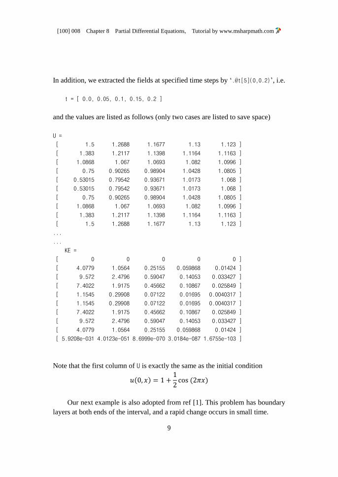
In addition we extracted the fields at specified time steps by lsquot[5](002)rsquo ie
t = [ 00 005 01 015 02 ]
and the values are listed as follows (only two cases are listed to save space)
U =
[ 15 12688 11677 113 1123 ]
[ 1383 12117 11398 11164 11163 ]
[ 10868 1067 10693 1082 10996 ]
[ 075 090265 098904 10428 10805 ]
[ 053015 079542 093671 10173 1068 ]
[ 053015 079542 093671 10173 1068 ]
[ 075 090265 098904 10428 10805 ]
[ 10868 1067 10693 1082 10996 ]
[ 1383 12117 11398 11164 11163 ]
[ 15 12688 11677 113 1123 ]
KE =
[ 0 0 0 0 0 ]
[ 40779 10564 025155 0059868 001424 ]
[ 9572 24796 059047 014053 0033427 ]
[ 74022 19175 045662 010867 0025849 ]
[ 11545 029908 007122 001695 00040317 ]
[ 11545 029908 007122 001695 00040317 ]
[ 74022 19175 045662 010867 0025849 ]
[ 9572 24796 059047 014053 0033427 ]
[ 40779 10564 025155 0059868 001424 ]
[ 59208e-031 40123e-051 86999e-070 30184e-087 16755e-103 ]
Note that the first column of U is exactly the same as the initial condition
Our next example is also adopted from ref [1] This problem has boundary
layers at both ends of the interval and a rapid change occurs in small time
[100] 008 Chapter 8 Partial Differential Equations Tutorial by wwwmsharpmathcom
10
where The initial conditions for
are
And the boundary conditions for are
Due to the presence of rapid change in time and the boundary layers in space
spanning numerical grids must reflect such behavior Therefore geometrically
increasing grid spans are employed
gt boundary layers and rapid change in small time
gt tout = [0 0005 001 005 01 05 1 15 2]
gt bvpt[2114](02) x[21-11](01) u = 1 v = 0
(
-u+0024u-( exp(573(u-v))-exp(-1146(u-v)) ) = 0
[ u = 0 u = 1 ]
-v+0170v+( exp(573(u-v))-exp(-1146(u-v)) ) = 0
[ v = 0 v = 0 ]
)
relax(04) maxiter(400) peep
plot[tout](u 2+v )
It should be noted that the function
is repeated for each equation This is because our solution is based on sequential
procedure and hence iteration is imposed at each time step Another feature
worthy of note is the use of Spoke lsquoplotrsquo If a pre-defined matrix is used inside
lsquo[ ]rsquo curves are selected from the corresponding times Numerical results are
shown in Figure 6
[100] 008 Chapter 8 Partial Differential Equations Tutorial by wwwmsharpmathcom
11
Figure 6 Solution to a system of PDs (u and v)
Section 8-2 Steady Elliptic PDEs
Steady elliptic PDEs involving two or three independent spatial variables
are treated here For generality three spatial coordinates are considered in
explaining Umbrella lsquopdersquo Nevertheless only licensed version can handle three
spatial coordinates
Standard Form The standard form of elliptic PDEs with three spatial
coordinates is written here as
where And are all of the same
sign from elliptic nature
To designate the partial derivatives our notations are innovated
[100] 008 Chapter 8 Partial Differential Equations Tutorial by wwwmsharpmathcom
12
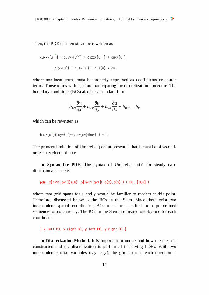
Then the PDE of interest can be rewritten as
cuxxu + cuyyu^^ + cuzzu~~ + cuxu
+ cuyu^ + cuzu~ + cuu = cs
where nonlinear terms must be properly expressed as coefficients or source
terms Those terms with lsquo rsquo are participating the discretization procedure The
boundary conditions (BCs) also has a standard form
which can be rewritten as
buxu+buyu^+buzu~+buu = bs
The primary limitation of Umbrella lsquopdersquo at present is that it must be of second-
order in each coordinate
Syntax for PDE The syntax of Umbrella lsquopdersquo for steady two-
dimensional space is
pde x[n=31g=1](ab) y[n=31g=1]( c(x)d(x) ) ( DE [BCs] )
where two grid spans for x and y would be familiar to readers at this point
Therefore discussed below is the BCs in the Stem Since there exist two
independent spatial coordinates BCs must be specified in a pre-defined
sequence for consistency The BCs in the Stem are treated one-by-one for each
coordinate
[ x-left BC x-right BC y-left BC y-right BC ]
Discretization Method It is important to understand how the mesh is
constructed and the discretization is performed in solving PDEs With two
independent spatial variables (say ) the grid span in each direction is
[100] 008 Chapter 8 Partial Differential Equations Tutorial by wwwmsharpmathcom
13
defined
Then the nodes for solution are selected to be the center of a quadrangle
enclosed by the four points
For boundaries the nodes for solution are selected to be the center of two
adjacent points It is worthy of note that the major weakness arises at four
corners of the whole domain since the solution at these corners are extrapolated
from the inside or the boundaries
Therefore for the syntax
pde x[m=31g=1](ab) y[n=31g=1]( c(x)d(x) ) ( DE [BCs] )
the mesh grid for computation has a dimension of This
means that the column of matrix represents
Single Elliptic PDE Our first example is very simple as shown below
which can be solved by
gt PDE of 2nd-order
gt pde x[10](01) y[10](01) (
u + u^^ + 10 = 0
[ u = 1 u = 1 u = 1 u = 1 ]
)
plot( u 0 )
[100] 008 Chapter 8 Partial Differential Equations Tutorial by wwwmsharpmathcom
14
The results are shown in Figure 7 Note that the computational mesh
corresponds to the field 0 and is shown in the right of Figure 7
Figure 7 Solution and mesh for a single PDE
As was mentioned above based on the pre-defined mesh
computational mesh of dimension is re-generated as shown in Figure
7 This is due to the treatment of control volume for discretizing the partial
differential equation The solution shown in the left of Figure 7 bears a
symmetry in both directions as expected
Comparison with Exact Solution Another example has an exact solution
The PDE of interest is written as
We solve this example by
gt PDE with exact solution
gt pde x[10](-11) y[10](-11) (
u + u^^ = 6
[ u = 1+2yy u = 1+2yy u = xx+2 u = xx+2 ]
)
plot( u -u+xx+2yy )
[100] 008 Chapter 8 Partial Differential Equations Tutorial by wwwmsharpmathcom
15
togo( Error = -u+xx+2yy )
gt Error
The u field is shown in Figure 8 and the error distribution is shown in Figure 9
Figure 8 A single PDE with exact solution
Figure 9 Error distribution
It is worthy of note that data at four corners are linearly extrapolated This is the
reason why there occur noticeable discrepancies at four corners in Figure 9
Conservative Form The second-order terms in some PDEs are
frequently expressed in conservative forms Thus we introduce the following
syntax for conservative forms
[100] 008 Chapter 8 Partial Differential Equations Tutorial by wwwmsharpmathcom
16
These conservative forms can be treated as long as they are the highest terms
This implies that either (p)u or u should appear once but not together
An example is
where
This PDE can be solved by
gt PDE in conservative form
gt pde xi[21](-11) eta[21]( -11 ) (
(exp(5xi)+1)u + (exp(5eta)+1)u^^ + 10 = 0
[ u = 0 u = 0 u = 0 u = 0 ]
)
plot(u)
And the result is shown in Figure 10
Figure 10 Conservative PDE
[100] 008 Chapter 8 Partial Differential Equations Tutorial by wwwmsharpmathcom
17
Next example is given below
where
For this example we employ non-uniform grid spans in both directions
gt PDE with nonuniform grid
gt pde x[21](-33) y[21]( -sqrt(10-xx)4-x2 ) (
(exp(x)+1)u + (exp(y)+1)u^^ + uu + u^ + u + 2 = 0
[ u = 0 u = 0 u = 0 u = 0 ]
)
plot(u)
And the result is shown in Figure 11
Figure 11 PDE in an irregular geometry
Section 8-3 System of Steady Elliptic PDEs
[100] 008 Chapter 8 Partial Differential Equations Tutorial by wwwmsharpmathcom
18
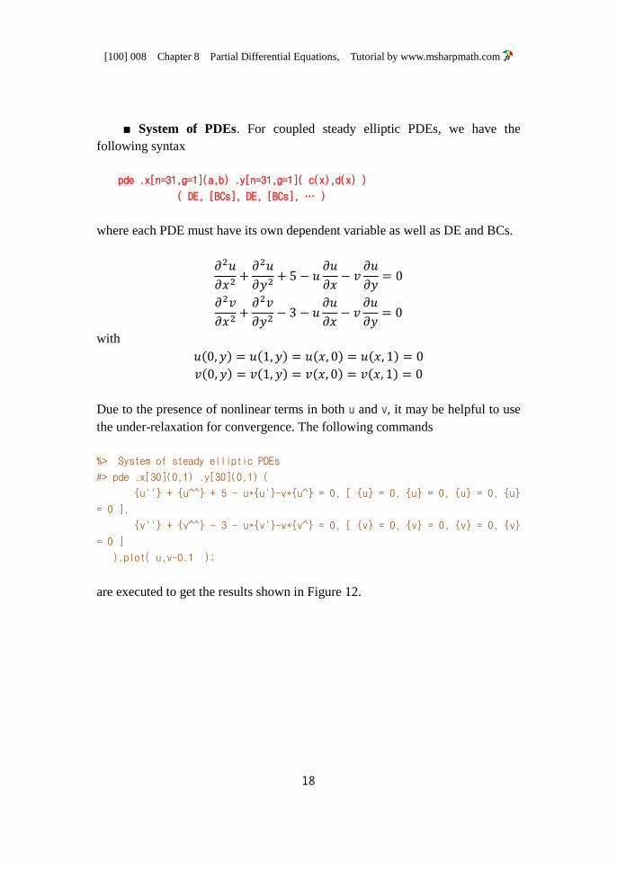
System of PDEs For coupled steady elliptic PDEs we have the
following syntax
pde x[n=31g=1](ab) y[n=31g=1]( c(x)d(x) )
( DE [BCs] DE [BCs] hellip )
where each PDE must have its own dependent variable as well as DE and BCs
with
Due to the presence of nonlinear terms in both u and v it may be helpful to use
the under-relaxation for convergence The following commands
gt System of steady elliptic PDEs
gt pde x[30](01) y[30](01) (
u + u^^ + 5 - uu-vu^ = 0 [ u = 0 u = 0 u = 0 u
= 0 ]
v + v^^ - 3 - uv-vv^ = 0 [ v = 0 v = 0 v = 0 v
= 0 ]
)plot( uv-01 )
are executed to get the results shown in Figure 12
[100] 008 Chapter 8 Partial Differential Equations Tutorial by wwwmsharpmathcom
19
Figure 12 system of PDEs
Section 8-4 Data Extraction
Spoke lsquotogorsquo To extract field data we use Spoke lsquotogorsquo as before To
illustrates this we consider again the first example discussed above
and the following Cemmath commands
gt Data extraction
gt pde x[4](01) y[5](01) (
u + u^^ + 5 = 0 [ u = 1 u = 1 u = 1 u = 1 ]
)
plot( u )
togo( X = x Y = y U = u )
gt X Y U
Note that lsquopde x[4](01) y[5](01)rsquo results in
mesh grid as shown in Figure 13
[100] 008 Chapter 8 Partial Differential Equations Tutorial by wwwmsharpmathcom
20
Figure 13 Data extraction
Data extraction for this case yields the following matrices
X =
[ 0 016667 05 083333 1 ]
[ 0 016667 05 083333 1 ]
[ 0 016667 05 083333 1 ]
[ 0 016667 05 083333 1 ]
[ 0 016667 05 083333 1 ]
[ 0 016667 05 083333 1 ]
Y =
[ 0 0 0 0 0 ]
[ 0125 0125 0125 0125 0125 ]
[ 0375 0375 0375 0375 0375 ]
[ 0625 0625 0625 0625 0625 ]
[ 0875 0875 0875 0875 0875 ]
[ 1 1 1 1 1 ]
U =
[ 1 1 1 1 1 ]
[ 1 11445 12063 11445 1 ]
[ 1 12487 13758 12487 1 ]
[ 1 12487 13758 12487 1 ]
[ 1 11445 12063 11445 1 ]
[ 1 1 1 1 1 ]
[100] 008 Chapter 8 Partial Differential Equations Tutorial by wwwmsharpmathcom
21
Section 8-5 Transient Elliptic PDEs
Syntax for PDE The syntax of Umbrella lsquopdersquo for transient two-
dimensional space is
pde t[ntime=31g=1](totf)
x[m=31g=1](ab) y[n=31g=1]( c(x)d(x) ) ( DE [BCs] )
where time must be the first grid span Spoke lsquotogorsquo for this case results in a
matrix of dimension
Therefore each column contains a field solution at a give time step
Single Transient PDE Our first example for a single transient PDE is
described as
which can be solved by
gt pdet[4](001)x[4](01)y[4](01) u=0 (
-u+u + u^^ + 10 = 0 [ u=0 u=0 u=0 u=0 ]
)
peep
plot[4]( u )
togo( U=u ) U
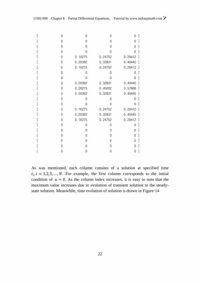
First the result from Spoke lsquotogorsquo is listed as
U =
[ 0 0 0 0 ]
[ 0 0 0 0 ]
[100] 008 Chapter 8 Partial Differential Equations Tutorial by wwwmsharpmathcom
22
[ 0 0 0 0 ]
[ 0 0 0 0 ]
[ 0 0 0 0 ]
[ 0 0 0 0 ]
[ 0 016275 024752 029412 ]
[ 0 020392 032831 040445 ]
[ 0 016275 024752 029412 ]
[ 0 0 0 0 ]
[ 0 0 0 0 ]
[ 0 020392 032831 040445 ]
[ 0 026275 045002 057668 ]
[ 0 020392 032831 040445 ]
[ 0 0 0 0 ]
[ 0 0 0 0 ]
[ 0 016275 024752 029412 ]
[ 0 020392 032831 040445 ]
[ 0 016275 024752 029412 ]
[ 0 0 0 0 ]
[ 0 0 0 0 ]
[ 0 0 0 0 ]
[ 0 0 0 0 ]
[ 0 0 0 0 ]
[ 0 0 0 0 ]
As was mentioned each column consists of a solution at specified time
For example the first column corresponds to the initial
condition of As the column index increases it is easy to note that the
maximum value increases due to evolution of transient solution to the steady-
state solution Meanwhile time evolution of solution is drawn in Figure 14
[100] 008 Chapter 8 Partial Differential Equations Tutorial by wwwmsharpmathcom
23
Figure 14 Time evolution of solution
System of Transient PDEs An example for a system of transient
elliptic PDEs is written below
With the initial condition
And the boundary conditions
This system of transient elliptic PDEs can be solved by
gt pde t[4](0015) x[30](01) y[30](01) u=0 v=1 (
-u - uu-vu^ + u + u^^ + 6 = 0
[100] 008 Chapter 8 Partial Differential Equations Tutorial by wwwmsharpmathcom
24
[ u=0 u=0 u=0 u=0 ]
-v - uv-vv^ + v + v^^ - 4 = 0
[ v=1 v=1 v=1 v=1 ]
) peepplot( uv ) uv
The results are shown in Figure 15
Figure 15 Time evolution of solution u and v
[100] 008 Chapter 8 Partial Differential Equations Tutorial by wwwmsharpmathcom
25
Section 8-6 Summary of Syntax
Syntax for Initial BVPs The syntax for initial BVPs is
bvp t[n=101g=1](tatb) x[n=101g=1](xaxb) IC ( DE [ BCs] )
pde x[m=31g=1](ab) y[n=31g=1]( c(x)d(x) ) ( DE [BCs] )
pde x[n=31g=1](ab)y[n=31g=1](c(x)d(x)) ( DE [BCs] DE [BCs])
pde x[n=31g=1](ab)y[n=31g=1](c(x)d(x)) ( DE [BCs] DE [BCs] )
pde t[ntime=31g=1](totf)
x[m=31g=1](ab) y[n=31g=1]( c(x)d(x) ) ( DE [BCs] )
Section 8-7 References
[1] DJ Higham and NJ Higham MATLAB(R) Program GuideBook 2ed
SIAM (2005)
[2] MATLAB(R) 7 Mathematics The MathWorks Inc (2009)
Page 2
[100] 008 Chapter 8 Partial Differential Equations Tutorial by wwwmsharpmathcom
2
respect to time Basically three partial derivatives with respect to time
can be handled in Cemmath where the prime denotes the partial differentiation
with respect to a spatial variable In using time derivatives such as f the first
independent variable of Hub must be time and proper IC should be prescribed
inside the Hub field
Single PDE Let us consider a single PDE the formulation of which is
discussed in ref [1]
where IC and BCs are given as
A first trial to solve this example over a range of 0 2t is
gt initial BVP
gt bvp t[21](02) x[21](01) Hub span
u = sin(pix) Hub field (initial condition)
( Stem
-pipiu + u = 0 partial differential equation
[ u = 0 piexp(-t)+u = 0 ] boundary conditions
)
peep plot2[6](u) Spoke
And Figure 1 displays six curves corresponding to Spoke lsquoplot2[6](u)rsquo
Regardless of the time span defined in the Hub span Spoke lsquoplot2[n=6g=1](u)rsquo
adopts its own time-span
[100] 008 Chapter 8 Partial Differential Equations Tutorial by wwwmsharpmathcom
3
for and otherwise The default values will be used if not
specified explicitly For this case time integration is primarily based on the
time grid specified as
bvp t[21](02)
which corresponds to t = [ 00 01 02 03 hellip 19 20 ] However time
nodes for plot are prescribed by lsquoplot2[6](u)rsquo which corresponds to t = [00
04 08 12 16 20 ] and six curves shown in Figure 1
Figure 1 Initial BVP
Using Spoke lsquoplotrsquo or lsquoplot3rsquo yields a three-dimensional plot Nevertheless
both lsquoplotrsquo and lsquoplot2rsquo cannot be used simultaneously The following
commands
gt initial BVP
gt bvp t[21](02) x[21](01)
u = sin(pix) (
pipiu - u = 0 [ u = 0 piexp(-t)+u = 0 ]
)
peep plot[6] ( u 2+01sinh(uu) )
illustrates the use of Spoke lsquoplotrsquo The results are presented in Figure 2 where
two surfaces corresponding to u and 01sinh(uu) are shown The surface on
[100] 008 Chapter 8 Partial Differential Equations Tutorial by wwwmsharpmathcom
4
the right of Figure 2 has no meaningful interpretation and is just prepared to
show the general capability of mathematical expressions for lsquoplotrsquo
Figure 2 3D plot for Initial BVP
Data Extraction The data fields in the numerical solution can be
extracted by using Spoke lsquotogorsquo For example let us consider again the PDE
discussed above
gt Data extraction for initial BVP
gt t = (02)span(4)
gt x = (01)span(5)
gt bvp [t][x] u = sin(pix) (
pipiu - u = 0
[ u = 0 piexp(-t)+u = 0 ]
) togo( X = x U = u Up = u Un = sqrt( uu+uu ) )
gt X U Up Un u
extract the fields x u u sqrt(uu+uu) and save them in corresponding
matrices as can be seen below
X =
[ 00000000 00000000 00000000 00000000 ]
[ 02500000 02500000 02500000 02500000 ]
[ 05000000 05000000 05000000 05000000 ]
[ 07500000 07500000 07500000 07500000 ]
[ 10000000 10000000 10000000 10000000 ]
U =
[ 00000000 00000000 00000000 00000000 ]
[100] 008 Chapter 8 Partial Differential Equations Tutorial by wwwmsharpmathcom
5
[ 07071068 04088247 02419403 01492274 ]
[ 10000000 05832507 03535360 02260789 ]
[ 07071068 04323081 02865326 02032533 ]
[ 00000000 00752341 01060874 01143207 ]
Up =
[ 36568542 19112923 11221755 06826950 ]
[ 20000000 13593053 08133469 05111245 ]
[ 00000000 00361025 00794188 01036875 ]
[ -20000000 -12436432 -06154460 -02862922 ]
[ -36568542 -16129484 -08281156 -04251691 ]
Un =
[ 36568542 19112923 11221755 06826950 ]
[ 21213203 14194536 08485684 05324632 ]
[ 10000000 05843670 03623466 02487223 ]
[ 21213203 13166392 06788775 03511056 ]
[ 36568542 16147021 08348832 04402704 ]
u =
[ 00000000 06826950 ]
[ 01492274 05111245 ]
[ 02260789 01036875 ]
[ 02032533 -02862922 ]
[ 01143207 -04251691 ]
The i -th column in each matrix corresponds to the field solution at time
where for this case In addition the variable u in the
Hub field contains u = [ u u ] at the final stage of solution The actual output
for u is
u =
[ 0 068269 ]
[ 014923 051112 ]
[ 022608 010369 ]
[ 020325 -028629 ]
[ 011432 -042517 ]
where is shown in the last element of the second
column as expected from BCs In prescribing IC it is also possible to specify
derivatives by the following syntax
[100] 008 Chapter 8 Partial Differential Equations Tutorial by wwwmsharpmathcom
6
u = [ u(x) u (x) ]
When the initial guess is given as u = u(x) derivatives of the initial guess are
evaluated internally with centered difference scheme Nevertheless it is wise to
specify the known mathematical expressions of derivatives for accuracy
improvement
Surface Plot Next example is the Black-Scholes PDE discussed in ref
[1]
where
And IC and BCs are given as
This example is solved by
gt Black-Scholes PDE
gt (rs) = (006508) k = r(s^22)
gt (ab) = (log(25)log(75)) (totf) = (05)
gt bvp t[11](totf) x[21](ab)
u = max(exp(x)-10) (
-u + u + (k-1)u - ku = 0
[ u = 0 u = (7-5exp(-kt))5 ]
)
peep plot[11](u)
And the results are shown in the left of Figure 3 Changing lsquoplotrsquo to lsquoplot2rsquo
[100] 008 Chapter 8 Partial Differential Equations Tutorial by wwwmsharpmathcom
7
yields a 2D plot shown in the right of Figure 3
Figure 3 3D and 2D plot for initial BVP
System of PDEs An example for a system of PDEs is taken from ref [1]
The PDEs are written as
where the initial conditions for are
And the boundary conditions for are
Since the utility of Umbrella is handling equations with minimum amount of
modification it is not surprising to note that the following Cemmath commands
gt system of initial BVP
gt bvp t[5](002) x[10](01) Hub span
u = [ 1+05cos(2pix) -pisin(2pix) ]
v = [ 1-05cos(2pix) pisin(2pix) ] Hub field
(
-u + 05u + 1(1+vv) = 0 [ u = 0 u = 0 ]
[100] 008 Chapter 8 Partial Differential Equations Tutorial by wwwmsharpmathcom
8
-v + 05v + 1(1+uu) = 0 [ v = 0 v = 0 ]
)peep
togo( U = u U1 = u V = v V1 = v KE = 05(uu+vv) )
plot[6](uv+2 4 + 05(uu+vv))
gt u v U U1 V V1 KE
produce the desired solutions The results are shown in Figure 4 and Figure 5
In particular the energy field defined as
is known to vanish as time approaches an infinity (see [ref 1]) Such a behavior
is represented in the energy field shown in Figure 5
Figure 4 Solution to a system of PDEs (u and v)
Figure 5 Solution to a system of PDEs (energy field)
[100] 008 Chapter 8 Partial Differential Equations Tutorial by wwwmsharpmathcom
9
In addition we extracted the fields at specified time steps by lsquot[5](002)rsquo ie
t = [ 00 005 01 015 02 ]
and the values are listed as follows (only two cases are listed to save space)
U =
[ 15 12688 11677 113 1123 ]
[ 1383 12117 11398 11164 11163 ]
[ 10868 1067 10693 1082 10996 ]
[ 075 090265 098904 10428 10805 ]
[ 053015 079542 093671 10173 1068 ]
[ 053015 079542 093671 10173 1068 ]
[ 075 090265 098904 10428 10805 ]
[ 10868 1067 10693 1082 10996 ]
[ 1383 12117 11398 11164 11163 ]
[ 15 12688 11677 113 1123 ]
KE =
[ 0 0 0 0 0 ]
[ 40779 10564 025155 0059868 001424 ]
[ 9572 24796 059047 014053 0033427 ]
[ 74022 19175 045662 010867 0025849 ]
[ 11545 029908 007122 001695 00040317 ]
[ 11545 029908 007122 001695 00040317 ]
[ 74022 19175 045662 010867 0025849 ]
[ 9572 24796 059047 014053 0033427 ]
[ 40779 10564 025155 0059868 001424 ]
[ 59208e-031 40123e-051 86999e-070 30184e-087 16755e-103 ]
Note that the first column of U is exactly the same as the initial condition
Our next example is also adopted from ref [1] This problem has boundary
layers at both ends of the interval and a rapid change occurs in small time
[100] 008 Chapter 8 Partial Differential Equations Tutorial by wwwmsharpmathcom
10
where The initial conditions for
are
And the boundary conditions for are
Due to the presence of rapid change in time and the boundary layers in space
spanning numerical grids must reflect such behavior Therefore geometrically
increasing grid spans are employed
gt boundary layers and rapid change in small time
gt tout = [0 0005 001 005 01 05 1 15 2]
gt bvpt[2114](02) x[21-11](01) u = 1 v = 0
(
-u+0024u-( exp(573(u-v))-exp(-1146(u-v)) ) = 0
[ u = 0 u = 1 ]
-v+0170v+( exp(573(u-v))-exp(-1146(u-v)) ) = 0
[ v = 0 v = 0 ]
)
relax(04) maxiter(400) peep
plot[tout](u 2+v )
It should be noted that the function
is repeated for each equation This is because our solution is based on sequential
procedure and hence iteration is imposed at each time step Another feature
worthy of note is the use of Spoke lsquoplotrsquo If a pre-defined matrix is used inside
lsquo[ ]rsquo curves are selected from the corresponding times Numerical results are
shown in Figure 6
[100] 008 Chapter 8 Partial Differential Equations Tutorial by wwwmsharpmathcom
11
Figure 6 Solution to a system of PDs (u and v)
Section 8-2 Steady Elliptic PDEs
Steady elliptic PDEs involving two or three independent spatial variables
are treated here For generality three spatial coordinates are considered in
explaining Umbrella lsquopdersquo Nevertheless only licensed version can handle three
spatial coordinates
Standard Form The standard form of elliptic PDEs with three spatial
coordinates is written here as
where And are all of the same
sign from elliptic nature
To designate the partial derivatives our notations are innovated
[100] 008 Chapter 8 Partial Differential Equations Tutorial by wwwmsharpmathcom
12
Then the PDE of interest can be rewritten as
cuxxu + cuyyu^^ + cuzzu~~ + cuxu
+ cuyu^ + cuzu~ + cuu = cs
where nonlinear terms must be properly expressed as coefficients or source
terms Those terms with lsquo rsquo are participating the discretization procedure The
boundary conditions (BCs) also has a standard form
which can be rewritten as
buxu+buyu^+buzu~+buu = bs
The primary limitation of Umbrella lsquopdersquo at present is that it must be of second-
order in each coordinate
Syntax for PDE The syntax of Umbrella lsquopdersquo for steady two-
dimensional space is
pde x[n=31g=1](ab) y[n=31g=1]( c(x)d(x) ) ( DE [BCs] )
where two grid spans for x and y would be familiar to readers at this point
Therefore discussed below is the BCs in the Stem Since there exist two
independent spatial coordinates BCs must be specified in a pre-defined
sequence for consistency The BCs in the Stem are treated one-by-one for each
coordinate
[ x-left BC x-right BC y-left BC y-right BC ]
Discretization Method It is important to understand how the mesh is
constructed and the discretization is performed in solving PDEs With two
independent spatial variables (say ) the grid span in each direction is
[100] 008 Chapter 8 Partial Differential Equations Tutorial by wwwmsharpmathcom
13
defined
Then the nodes for solution are selected to be the center of a quadrangle
enclosed by the four points
For boundaries the nodes for solution are selected to be the center of two
adjacent points It is worthy of note that the major weakness arises at four
corners of the whole domain since the solution at these corners are extrapolated
from the inside or the boundaries
Therefore for the syntax
pde x[m=31g=1](ab) y[n=31g=1]( c(x)d(x) ) ( DE [BCs] )
the mesh grid for computation has a dimension of This
means that the column of matrix represents
Single Elliptic PDE Our first example is very simple as shown below
which can be solved by
gt PDE of 2nd-order
gt pde x[10](01) y[10](01) (
u + u^^ + 10 = 0
[ u = 1 u = 1 u = 1 u = 1 ]
)
plot( u 0 )
[100] 008 Chapter 8 Partial Differential Equations Tutorial by wwwmsharpmathcom
14
The results are shown in Figure 7 Note that the computational mesh
corresponds to the field 0 and is shown in the right of Figure 7
Figure 7 Solution and mesh for a single PDE
As was mentioned above based on the pre-defined mesh
computational mesh of dimension is re-generated as shown in Figure
7 This is due to the treatment of control volume for discretizing the partial
differential equation The solution shown in the left of Figure 7 bears a
symmetry in both directions as expected
Comparison with Exact Solution Another example has an exact solution
The PDE of interest is written as
We solve this example by
gt PDE with exact solution
gt pde x[10](-11) y[10](-11) (
u + u^^ = 6
[ u = 1+2yy u = 1+2yy u = xx+2 u = xx+2 ]
)
plot( u -u+xx+2yy )
[100] 008 Chapter 8 Partial Differential Equations Tutorial by wwwmsharpmathcom
15
togo( Error = -u+xx+2yy )
gt Error
The u field is shown in Figure 8 and the error distribution is shown in Figure 9
Figure 8 A single PDE with exact solution
Figure 9 Error distribution
It is worthy of note that data at four corners are linearly extrapolated This is the
reason why there occur noticeable discrepancies at four corners in Figure 9
Conservative Form The second-order terms in some PDEs are
frequently expressed in conservative forms Thus we introduce the following
syntax for conservative forms
[100] 008 Chapter 8 Partial Differential Equations Tutorial by wwwmsharpmathcom
16
These conservative forms can be treated as long as they are the highest terms
This implies that either (p)u or u should appear once but not together
An example is
where
This PDE can be solved by
gt PDE in conservative form
gt pde xi[21](-11) eta[21]( -11 ) (
(exp(5xi)+1)u + (exp(5eta)+1)u^^ + 10 = 0
[ u = 0 u = 0 u = 0 u = 0 ]
)
plot(u)
And the result is shown in Figure 10
Figure 10 Conservative PDE
[100] 008 Chapter 8 Partial Differential Equations Tutorial by wwwmsharpmathcom
17
Next example is given below
where
For this example we employ non-uniform grid spans in both directions
gt PDE with nonuniform grid
gt pde x[21](-33) y[21]( -sqrt(10-xx)4-x2 ) (
(exp(x)+1)u + (exp(y)+1)u^^ + uu + u^ + u + 2 = 0
[ u = 0 u = 0 u = 0 u = 0 ]
)
plot(u)
And the result is shown in Figure 11
Figure 11 PDE in an irregular geometry
Section 8-3 System of Steady Elliptic PDEs
[100] 008 Chapter 8 Partial Differential Equations Tutorial by wwwmsharpmathcom
18
System of PDEs For coupled steady elliptic PDEs we have the
following syntax
pde x[n=31g=1](ab) y[n=31g=1]( c(x)d(x) )
( DE [BCs] DE [BCs] hellip )
where each PDE must have its own dependent variable as well as DE and BCs
with
Due to the presence of nonlinear terms in both u and v it may be helpful to use
the under-relaxation for convergence The following commands
gt System of steady elliptic PDEs
gt pde x[30](01) y[30](01) (
u + u^^ + 5 - uu-vu^ = 0 [ u = 0 u = 0 u = 0 u
= 0 ]
v + v^^ - 3 - uv-vv^ = 0 [ v = 0 v = 0 v = 0 v
= 0 ]
)plot( uv-01 )
are executed to get the results shown in Figure 12
[100] 008 Chapter 8 Partial Differential Equations Tutorial by wwwmsharpmathcom
19
Figure 12 system of PDEs
Section 8-4 Data Extraction
Spoke lsquotogorsquo To extract field data we use Spoke lsquotogorsquo as before To
illustrates this we consider again the first example discussed above
and the following Cemmath commands
gt Data extraction
gt pde x[4](01) y[5](01) (
u + u^^ + 5 = 0 [ u = 1 u = 1 u = 1 u = 1 ]
)
plot( u )
togo( X = x Y = y U = u )
gt X Y U
Note that lsquopde x[4](01) y[5](01)rsquo results in
mesh grid as shown in Figure 13
[100] 008 Chapter 8 Partial Differential Equations Tutorial by wwwmsharpmathcom
20
Figure 13 Data extraction
Data extraction for this case yields the following matrices
X =
[ 0 016667 05 083333 1 ]
[ 0 016667 05 083333 1 ]
[ 0 016667 05 083333 1 ]
[ 0 016667 05 083333 1 ]
[ 0 016667 05 083333 1 ]
[ 0 016667 05 083333 1 ]
Y =
[ 0 0 0 0 0 ]
[ 0125 0125 0125 0125 0125 ]
[ 0375 0375 0375 0375 0375 ]
[ 0625 0625 0625 0625 0625 ]
[ 0875 0875 0875 0875 0875 ]
[ 1 1 1 1 1 ]
U =
[ 1 1 1 1 1 ]
[ 1 11445 12063 11445 1 ]
[ 1 12487 13758 12487 1 ]
[ 1 12487 13758 12487 1 ]
[ 1 11445 12063 11445 1 ]
[ 1 1 1 1 1 ]
[100] 008 Chapter 8 Partial Differential Equations Tutorial by wwwmsharpmathcom
21
Section 8-5 Transient Elliptic PDEs
Syntax for PDE The syntax of Umbrella lsquopdersquo for transient two-
dimensional space is
pde t[ntime=31g=1](totf)
x[m=31g=1](ab) y[n=31g=1]( c(x)d(x) ) ( DE [BCs] )
where time must be the first grid span Spoke lsquotogorsquo for this case results in a
matrix of dimension
Therefore each column contains a field solution at a give time step
Single Transient PDE Our first example for a single transient PDE is
described as
which can be solved by
gt pdet[4](001)x[4](01)y[4](01) u=0 (
-u+u + u^^ + 10 = 0 [ u=0 u=0 u=0 u=0 ]
)
peep
plot[4]( u )
togo( U=u ) U
First the result from Spoke lsquotogorsquo is listed as
U =
[ 0 0 0 0 ]
[ 0 0 0 0 ]
[100] 008 Chapter 8 Partial Differential Equations Tutorial by wwwmsharpmathcom
22
[ 0 0 0 0 ]
[ 0 0 0 0 ]
[ 0 0 0 0 ]
[ 0 0 0 0 ]
[ 0 016275 024752 029412 ]
[ 0 020392 032831 040445 ]
[ 0 016275 024752 029412 ]
[ 0 0 0 0 ]
[ 0 0 0 0 ]
[ 0 020392 032831 040445 ]
[ 0 026275 045002 057668 ]
[ 0 020392 032831 040445 ]
[ 0 0 0 0 ]
[ 0 0 0 0 ]
[ 0 016275 024752 029412 ]
[ 0 020392 032831 040445 ]
[ 0 016275 024752 029412 ]
[ 0 0 0 0 ]
[ 0 0 0 0 ]
[ 0 0 0 0 ]
[ 0 0 0 0 ]
[ 0 0 0 0 ]
[ 0 0 0 0 ]
As was mentioned each column consists of a solution at specified time
For example the first column corresponds to the initial
condition of As the column index increases it is easy to note that the
maximum value increases due to evolution of transient solution to the steady-
state solution Meanwhile time evolution of solution is drawn in Figure 14
[100] 008 Chapter 8 Partial Differential Equations Tutorial by wwwmsharpmathcom
23
Figure 14 Time evolution of solution
System of Transient PDEs An example for a system of transient
elliptic PDEs is written below
With the initial condition
And the boundary conditions
This system of transient elliptic PDEs can be solved by
gt pde t[4](0015) x[30](01) y[30](01) u=0 v=1 (
-u - uu-vu^ + u + u^^ + 6 = 0
[100] 008 Chapter 8 Partial Differential Equations Tutorial by wwwmsharpmathcom
24
[ u=0 u=0 u=0 u=0 ]
-v - uv-vv^ + v + v^^ - 4 = 0
[ v=1 v=1 v=1 v=1 ]
) peepplot( uv ) uv
The results are shown in Figure 15
Figure 15 Time evolution of solution u and v
[100] 008 Chapter 8 Partial Differential Equations Tutorial by wwwmsharpmathcom
25
Section 8-6 Summary of Syntax
Syntax for Initial BVPs The syntax for initial BVPs is
bvp t[n=101g=1](tatb) x[n=101g=1](xaxb) IC ( DE [ BCs] )
pde x[m=31g=1](ab) y[n=31g=1]( c(x)d(x) ) ( DE [BCs] )
pde x[n=31g=1](ab)y[n=31g=1](c(x)d(x)) ( DE [BCs] DE [BCs])
pde x[n=31g=1](ab)y[n=31g=1](c(x)d(x)) ( DE [BCs] DE [BCs] )
pde t[ntime=31g=1](totf)
x[m=31g=1](ab) y[n=31g=1]( c(x)d(x) ) ( DE [BCs] )
Section 8-7 References
[1] DJ Higham and NJ Higham MATLAB(R) Program GuideBook 2ed
SIAM (2005)
[2] MATLAB(R) 7 Mathematics The MathWorks Inc (2009)
Page 3
[100] 008 Chapter 8 Partial Differential Equations Tutorial by wwwmsharpmathcom
3
for and otherwise The default values will be used if not
specified explicitly For this case time integration is primarily based on the
time grid specified as
bvp t[21](02)
which corresponds to t = [ 00 01 02 03 hellip 19 20 ] However time
nodes for plot are prescribed by lsquoplot2[6](u)rsquo which corresponds to t = [00
04 08 12 16 20 ] and six curves shown in Figure 1
Figure 1 Initial BVP
Using Spoke lsquoplotrsquo or lsquoplot3rsquo yields a three-dimensional plot Nevertheless
both lsquoplotrsquo and lsquoplot2rsquo cannot be used simultaneously The following
commands
gt initial BVP
gt bvp t[21](02) x[21](01)
u = sin(pix) (
pipiu - u = 0 [ u = 0 piexp(-t)+u = 0 ]
)
peep plot[6] ( u 2+01sinh(uu) )
illustrates the use of Spoke lsquoplotrsquo The results are presented in Figure 2 where
two surfaces corresponding to u and 01sinh(uu) are shown The surface on
[100] 008 Chapter 8 Partial Differential Equations Tutorial by wwwmsharpmathcom
4
the right of Figure 2 has no meaningful interpretation and is just prepared to
show the general capability of mathematical expressions for lsquoplotrsquo
Figure 2 3D plot for Initial BVP
Data Extraction The data fields in the numerical solution can be
extracted by using Spoke lsquotogorsquo For example let us consider again the PDE
discussed above
gt Data extraction for initial BVP
gt t = (02)span(4)
gt x = (01)span(5)
gt bvp [t][x] u = sin(pix) (
pipiu - u = 0
[ u = 0 piexp(-t)+u = 0 ]
) togo( X = x U = u Up = u Un = sqrt( uu+uu ) )
gt X U Up Un u
extract the fields x u u sqrt(uu+uu) and save them in corresponding
matrices as can be seen below
X =
[ 00000000 00000000 00000000 00000000 ]
[ 02500000 02500000 02500000 02500000 ]
[ 05000000 05000000 05000000 05000000 ]
[ 07500000 07500000 07500000 07500000 ]
[ 10000000 10000000 10000000 10000000 ]
U =
[ 00000000 00000000 00000000 00000000 ]
[100] 008 Chapter 8 Partial Differential Equations Tutorial by wwwmsharpmathcom
5
[ 07071068 04088247 02419403 01492274 ]
[ 10000000 05832507 03535360 02260789 ]
[ 07071068 04323081 02865326 02032533 ]
[ 00000000 00752341 01060874 01143207 ]
Up =
[ 36568542 19112923 11221755 06826950 ]
[ 20000000 13593053 08133469 05111245 ]
[ 00000000 00361025 00794188 01036875 ]
[ -20000000 -12436432 -06154460 -02862922 ]
[ -36568542 -16129484 -08281156 -04251691 ]
Un =
[ 36568542 19112923 11221755 06826950 ]
[ 21213203 14194536 08485684 05324632 ]
[ 10000000 05843670 03623466 02487223 ]
[ 21213203 13166392 06788775 03511056 ]
[ 36568542 16147021 08348832 04402704 ]
u =
[ 00000000 06826950 ]
[ 01492274 05111245 ]
[ 02260789 01036875 ]
[ 02032533 -02862922 ]
[ 01143207 -04251691 ]
The i -th column in each matrix corresponds to the field solution at time
where for this case In addition the variable u in the
Hub field contains u = [ u u ] at the final stage of solution The actual output
for u is
u =
[ 0 068269 ]
[ 014923 051112 ]
[ 022608 010369 ]
[ 020325 -028629 ]
[ 011432 -042517 ]
where is shown in the last element of the second
column as expected from BCs In prescribing IC it is also possible to specify
derivatives by the following syntax
[100] 008 Chapter 8 Partial Differential Equations Tutorial by wwwmsharpmathcom
6
u = [ u(x) u (x) ]
When the initial guess is given as u = u(x) derivatives of the initial guess are
evaluated internally with centered difference scheme Nevertheless it is wise to
specify the known mathematical expressions of derivatives for accuracy
improvement
Surface Plot Next example is the Black-Scholes PDE discussed in ref
[1]
where
And IC and BCs are given as
This example is solved by
gt Black-Scholes PDE
gt (rs) = (006508) k = r(s^22)
gt (ab) = (log(25)log(75)) (totf) = (05)
gt bvp t[11](totf) x[21](ab)
u = max(exp(x)-10) (
-u + u + (k-1)u - ku = 0
[ u = 0 u = (7-5exp(-kt))5 ]
)
peep plot[11](u)
And the results are shown in the left of Figure 3 Changing lsquoplotrsquo to lsquoplot2rsquo
[100] 008 Chapter 8 Partial Differential Equations Tutorial by wwwmsharpmathcom
7
yields a 2D plot shown in the right of Figure 3
Figure 3 3D and 2D plot for initial BVP
System of PDEs An example for a system of PDEs is taken from ref [1]
The PDEs are written as
where the initial conditions for are
And the boundary conditions for are
Since the utility of Umbrella is handling equations with minimum amount of
modification it is not surprising to note that the following Cemmath commands
gt system of initial BVP
gt bvp t[5](002) x[10](01) Hub span
u = [ 1+05cos(2pix) -pisin(2pix) ]
v = [ 1-05cos(2pix) pisin(2pix) ] Hub field
(
-u + 05u + 1(1+vv) = 0 [ u = 0 u = 0 ]
[100] 008 Chapter 8 Partial Differential Equations Tutorial by wwwmsharpmathcom
8
-v + 05v + 1(1+uu) = 0 [ v = 0 v = 0 ]
)peep
togo( U = u U1 = u V = v V1 = v KE = 05(uu+vv) )
plot[6](uv+2 4 + 05(uu+vv))
gt u v U U1 V V1 KE
produce the desired solutions The results are shown in Figure 4 and Figure 5
In particular the energy field defined as
is known to vanish as time approaches an infinity (see [ref 1]) Such a behavior
is represented in the energy field shown in Figure 5
Figure 4 Solution to a system of PDEs (u and v)
Figure 5 Solution to a system of PDEs (energy field)
[100] 008 Chapter 8 Partial Differential Equations Tutorial by wwwmsharpmathcom
9
In addition we extracted the fields at specified time steps by lsquot[5](002)rsquo ie
t = [ 00 005 01 015 02 ]
and the values are listed as follows (only two cases are listed to save space)
U =
[ 15 12688 11677 113 1123 ]
[ 1383 12117 11398 11164 11163 ]
[ 10868 1067 10693 1082 10996 ]
[ 075 090265 098904 10428 10805 ]
[ 053015 079542 093671 10173 1068 ]
[ 053015 079542 093671 10173 1068 ]
[ 075 090265 098904 10428 10805 ]
[ 10868 1067 10693 1082 10996 ]
[ 1383 12117 11398 11164 11163 ]
[ 15 12688 11677 113 1123 ]
KE =
[ 0 0 0 0 0 ]
[ 40779 10564 025155 0059868 001424 ]
[ 9572 24796 059047 014053 0033427 ]
[ 74022 19175 045662 010867 0025849 ]
[ 11545 029908 007122 001695 00040317 ]
[ 11545 029908 007122 001695 00040317 ]
[ 74022 19175 045662 010867 0025849 ]
[ 9572 24796 059047 014053 0033427 ]
[ 40779 10564 025155 0059868 001424 ]
[ 59208e-031 40123e-051 86999e-070 30184e-087 16755e-103 ]
Note that the first column of U is exactly the same as the initial condition
Our next example is also adopted from ref [1] This problem has boundary
layers at both ends of the interval and a rapid change occurs in small time
[100] 008 Chapter 8 Partial Differential Equations Tutorial by wwwmsharpmathcom
10
where The initial conditions for
are
And the boundary conditions for are
Due to the presence of rapid change in time and the boundary layers in space
spanning numerical grids must reflect such behavior Therefore geometrically
increasing grid spans are employed
gt boundary layers and rapid change in small time
gt tout = [0 0005 001 005 01 05 1 15 2]
gt bvpt[2114](02) x[21-11](01) u = 1 v = 0
(
-u+0024u-( exp(573(u-v))-exp(-1146(u-v)) ) = 0
[ u = 0 u = 1 ]
-v+0170v+( exp(573(u-v))-exp(-1146(u-v)) ) = 0
[ v = 0 v = 0 ]
)
relax(04) maxiter(400) peep
plot[tout](u 2+v )
It should be noted that the function
is repeated for each equation This is because our solution is based on sequential
procedure and hence iteration is imposed at each time step Another feature
worthy of note is the use of Spoke lsquoplotrsquo If a pre-defined matrix is used inside
lsquo[ ]rsquo curves are selected from the corresponding times Numerical results are
shown in Figure 6
[100] 008 Chapter 8 Partial Differential Equations Tutorial by wwwmsharpmathcom
11
Figure 6 Solution to a system of PDs (u and v)
Section 8-2 Steady Elliptic PDEs
Steady elliptic PDEs involving two or three independent spatial variables
are treated here For generality three spatial coordinates are considered in
explaining Umbrella lsquopdersquo Nevertheless only licensed version can handle three
spatial coordinates
Standard Form The standard form of elliptic PDEs with three spatial
coordinates is written here as
where And are all of the same
sign from elliptic nature
To designate the partial derivatives our notations are innovated
[100] 008 Chapter 8 Partial Differential Equations Tutorial by wwwmsharpmathcom
12
Then the PDE of interest can be rewritten as
cuxxu + cuyyu^^ + cuzzu~~ + cuxu
+ cuyu^ + cuzu~ + cuu = cs
where nonlinear terms must be properly expressed as coefficients or source
terms Those terms with lsquo rsquo are participating the discretization procedure The
boundary conditions (BCs) also has a standard form
which can be rewritten as
buxu+buyu^+buzu~+buu = bs
The primary limitation of Umbrella lsquopdersquo at present is that it must be of second-
order in each coordinate
Syntax for PDE The syntax of Umbrella lsquopdersquo for steady two-
dimensional space is
pde x[n=31g=1](ab) y[n=31g=1]( c(x)d(x) ) ( DE [BCs] )
where two grid spans for x and y would be familiar to readers at this point
Therefore discussed below is the BCs in the Stem Since there exist two
independent spatial coordinates BCs must be specified in a pre-defined
sequence for consistency The BCs in the Stem are treated one-by-one for each
coordinate
[ x-left BC x-right BC y-left BC y-right BC ]
Discretization Method It is important to understand how the mesh is
constructed and the discretization is performed in solving PDEs With two
independent spatial variables (say ) the grid span in each direction is
[100] 008 Chapter 8 Partial Differential Equations Tutorial by wwwmsharpmathcom
13
defined
Then the nodes for solution are selected to be the center of a quadrangle
enclosed by the four points
For boundaries the nodes for solution are selected to be the center of two
adjacent points It is worthy of note that the major weakness arises at four
corners of the whole domain since the solution at these corners are extrapolated
from the inside or the boundaries
Therefore for the syntax
pde x[m=31g=1](ab) y[n=31g=1]( c(x)d(x) ) ( DE [BCs] )
the mesh grid for computation has a dimension of This
means that the column of matrix represents
Single Elliptic PDE Our first example is very simple as shown below
which can be solved by
gt PDE of 2nd-order
gt pde x[10](01) y[10](01) (
u + u^^ + 10 = 0
[ u = 1 u = 1 u = 1 u = 1 ]
)
plot( u 0 )
[100] 008 Chapter 8 Partial Differential Equations Tutorial by wwwmsharpmathcom
14
The results are shown in Figure 7 Note that the computational mesh
corresponds to the field 0 and is shown in the right of Figure 7
Figure 7 Solution and mesh for a single PDE
As was mentioned above based on the pre-defined mesh
computational mesh of dimension is re-generated as shown in Figure
7 This is due to the treatment of control volume for discretizing the partial
differential equation The solution shown in the left of Figure 7 bears a
symmetry in both directions as expected
Comparison with Exact Solution Another example has an exact solution
The PDE of interest is written as
We solve this example by
gt PDE with exact solution
gt pde x[10](-11) y[10](-11) (
u + u^^ = 6
[ u = 1+2yy u = 1+2yy u = xx+2 u = xx+2 ]
)
plot( u -u+xx+2yy )
[100] 008 Chapter 8 Partial Differential Equations Tutorial by wwwmsharpmathcom
15
togo( Error = -u+xx+2yy )
gt Error
The u field is shown in Figure 8 and the error distribution is shown in Figure 9
Figure 8 A single PDE with exact solution
Figure 9 Error distribution
It is worthy of note that data at four corners are linearly extrapolated This is the
reason why there occur noticeable discrepancies at four corners in Figure 9
Conservative Form The second-order terms in some PDEs are
frequently expressed in conservative forms Thus we introduce the following
syntax for conservative forms
[100] 008 Chapter 8 Partial Differential Equations Tutorial by wwwmsharpmathcom
16
These conservative forms can be treated as long as they are the highest terms
This implies that either (p)u or u should appear once but not together
An example is
where
This PDE can be solved by
gt PDE in conservative form
gt pde xi[21](-11) eta[21]( -11 ) (
(exp(5xi)+1)u + (exp(5eta)+1)u^^ + 10 = 0
[ u = 0 u = 0 u = 0 u = 0 ]
)
plot(u)
And the result is shown in Figure 10
Figure 10 Conservative PDE
[100] 008 Chapter 8 Partial Differential Equations Tutorial by wwwmsharpmathcom
17
Next example is given below
where
For this example we employ non-uniform grid spans in both directions
gt PDE with nonuniform grid
gt pde x[21](-33) y[21]( -sqrt(10-xx)4-x2 ) (
(exp(x)+1)u + (exp(y)+1)u^^ + uu + u^ + u + 2 = 0
[ u = 0 u = 0 u = 0 u = 0 ]
)
plot(u)
And the result is shown in Figure 11
Figure 11 PDE in an irregular geometry
Section 8-3 System of Steady Elliptic PDEs
[100] 008 Chapter 8 Partial Differential Equations Tutorial by wwwmsharpmathcom
18
System of PDEs For coupled steady elliptic PDEs we have the
following syntax
pde x[n=31g=1](ab) y[n=31g=1]( c(x)d(x) )
( DE [BCs] DE [BCs] hellip )
where each PDE must have its own dependent variable as well as DE and BCs
with
Due to the presence of nonlinear terms in both u and v it may be helpful to use
the under-relaxation for convergence The following commands
gt System of steady elliptic PDEs
gt pde x[30](01) y[30](01) (
u + u^^ + 5 - uu-vu^ = 0 [ u = 0 u = 0 u = 0 u
= 0 ]
v + v^^ - 3 - uv-vv^ = 0 [ v = 0 v = 0 v = 0 v
= 0 ]
)plot( uv-01 )
are executed to get the results shown in Figure 12
[100] 008 Chapter 8 Partial Differential Equations Tutorial by wwwmsharpmathcom
19
Figure 12 system of PDEs
Section 8-4 Data Extraction
Spoke lsquotogorsquo To extract field data we use Spoke lsquotogorsquo as before To
illustrates this we consider again the first example discussed above
and the following Cemmath commands
gt Data extraction
gt pde x[4](01) y[5](01) (
u + u^^ + 5 = 0 [ u = 1 u = 1 u = 1 u = 1 ]
)
plot( u )
togo( X = x Y = y U = u )
gt X Y U
Note that lsquopde x[4](01) y[5](01)rsquo results in
mesh grid as shown in Figure 13
[100] 008 Chapter 8 Partial Differential Equations Tutorial by wwwmsharpmathcom
20
Figure 13 Data extraction
Data extraction for this case yields the following matrices
X =
[ 0 016667 05 083333 1 ]
[ 0 016667 05 083333 1 ]
[ 0 016667 05 083333 1 ]
[ 0 016667 05 083333 1 ]
[ 0 016667 05 083333 1 ]
[ 0 016667 05 083333 1 ]
Y =
[ 0 0 0 0 0 ]
[ 0125 0125 0125 0125 0125 ]
[ 0375 0375 0375 0375 0375 ]
[ 0625 0625 0625 0625 0625 ]
[ 0875 0875 0875 0875 0875 ]
[ 1 1 1 1 1 ]
U =
[ 1 1 1 1 1 ]
[ 1 11445 12063 11445 1 ]
[ 1 12487 13758 12487 1 ]
[ 1 12487 13758 12487 1 ]
[ 1 11445 12063 11445 1 ]
[ 1 1 1 1 1 ]
[100] 008 Chapter 8 Partial Differential Equations Tutorial by wwwmsharpmathcom
21
Section 8-5 Transient Elliptic PDEs
Syntax for PDE The syntax of Umbrella lsquopdersquo for transient two-
dimensional space is
pde t[ntime=31g=1](totf)
x[m=31g=1](ab) y[n=31g=1]( c(x)d(x) ) ( DE [BCs] )
where time must be the first grid span Spoke lsquotogorsquo for this case results in a
matrix of dimension
Therefore each column contains a field solution at a give time step
Single Transient PDE Our first example for a single transient PDE is
described as
which can be solved by
gt pdet[4](001)x[4](01)y[4](01) u=0 (
-u+u + u^^ + 10 = 0 [ u=0 u=0 u=0 u=0 ]
)
peep
plot[4]( u )
togo( U=u ) U
First the result from Spoke lsquotogorsquo is listed as
U =
[ 0 0 0 0 ]
[ 0 0 0 0 ]
[100] 008 Chapter 8 Partial Differential Equations Tutorial by wwwmsharpmathcom
22
[ 0 0 0 0 ]
[ 0 0 0 0 ]
[ 0 0 0 0 ]
[ 0 0 0 0 ]
[ 0 016275 024752 029412 ]
[ 0 020392 032831 040445 ]
[ 0 016275 024752 029412 ]
[ 0 0 0 0 ]
[ 0 0 0 0 ]
[ 0 020392 032831 040445 ]
[ 0 026275 045002 057668 ]
[ 0 020392 032831 040445 ]
[ 0 0 0 0 ]
[ 0 0 0 0 ]
[ 0 016275 024752 029412 ]
[ 0 020392 032831 040445 ]
[ 0 016275 024752 029412 ]
[ 0 0 0 0 ]
[ 0 0 0 0 ]
[ 0 0 0 0 ]
[ 0 0 0 0 ]
[ 0 0 0 0 ]
[ 0 0 0 0 ]
As was mentioned each column consists of a solution at specified time
For example the first column corresponds to the initial
condition of As the column index increases it is easy to note that the
maximum value increases due to evolution of transient solution to the steady-
state solution Meanwhile time evolution of solution is drawn in Figure 14
[100] 008 Chapter 8 Partial Differential Equations Tutorial by wwwmsharpmathcom
23
Figure 14 Time evolution of solution
System of Transient PDEs An example for a system of transient
elliptic PDEs is written below
With the initial condition
And the boundary conditions
This system of transient elliptic PDEs can be solved by
gt pde t[4](0015) x[30](01) y[30](01) u=0 v=1 (
-u - uu-vu^ + u + u^^ + 6 = 0
[100] 008 Chapter 8 Partial Differential Equations Tutorial by wwwmsharpmathcom
24
[ u=0 u=0 u=0 u=0 ]
-v - uv-vv^ + v + v^^ - 4 = 0
[ v=1 v=1 v=1 v=1 ]
) peepplot( uv ) uv
The results are shown in Figure 15
Figure 15 Time evolution of solution u and v
[100] 008 Chapter 8 Partial Differential Equations Tutorial by wwwmsharpmathcom
25
Section 8-6 Summary of Syntax
Syntax for Initial BVPs The syntax for initial BVPs is
bvp t[n=101g=1](tatb) x[n=101g=1](xaxb) IC ( DE [ BCs] )
pde x[m=31g=1](ab) y[n=31g=1]( c(x)d(x) ) ( DE [BCs] )
pde x[n=31g=1](ab)y[n=31g=1](c(x)d(x)) ( DE [BCs] DE [BCs])
pde x[n=31g=1](ab)y[n=31g=1](c(x)d(x)) ( DE [BCs] DE [BCs] )
pde t[ntime=31g=1](totf)
x[m=31g=1](ab) y[n=31g=1]( c(x)d(x) ) ( DE [BCs] )
Section 8-7 References
[1] DJ Higham and NJ Higham MATLAB(R) Program GuideBook 2ed
SIAM (2005)
[2] MATLAB(R) 7 Mathematics The MathWorks Inc (2009)
Page 4
[100] 008 Chapter 8 Partial Differential Equations Tutorial by wwwmsharpmathcom
4
the right of Figure 2 has no meaningful interpretation and is just prepared to
show the general capability of mathematical expressions for lsquoplotrsquo
Figure 2 3D plot for Initial BVP
Data Extraction The data fields in the numerical solution can be
extracted by using Spoke lsquotogorsquo For example let us consider again the PDE
discussed above
gt Data extraction for initial BVP
gt t = (02)span(4)
gt x = (01)span(5)
gt bvp [t][x] u = sin(pix) (
pipiu - u = 0
[ u = 0 piexp(-t)+u = 0 ]
) togo( X = x U = u Up = u Un = sqrt( uu+uu ) )
gt X U Up Un u
extract the fields x u u sqrt(uu+uu) and save them in corresponding
matrices as can be seen below
X =
[ 00000000 00000000 00000000 00000000 ]
[ 02500000 02500000 02500000 02500000 ]
[ 05000000 05000000 05000000 05000000 ]
[ 07500000 07500000 07500000 07500000 ]
[ 10000000 10000000 10000000 10000000 ]
U =
[ 00000000 00000000 00000000 00000000 ]
[100] 008 Chapter 8 Partial Differential Equations Tutorial by wwwmsharpmathcom
5
[ 07071068 04088247 02419403 01492274 ]
[ 10000000 05832507 03535360 02260789 ]
[ 07071068 04323081 02865326 02032533 ]
[ 00000000 00752341 01060874 01143207 ]
Up =
[ 36568542 19112923 11221755 06826950 ]
[ 20000000 13593053 08133469 05111245 ]
[ 00000000 00361025 00794188 01036875 ]
[ -20000000 -12436432 -06154460 -02862922 ]
[ -36568542 -16129484 -08281156 -04251691 ]
Un =
[ 36568542 19112923 11221755 06826950 ]
[ 21213203 14194536 08485684 05324632 ]
[ 10000000 05843670 03623466 02487223 ]
[ 21213203 13166392 06788775 03511056 ]
[ 36568542 16147021 08348832 04402704 ]
u =
[ 00000000 06826950 ]
[ 01492274 05111245 ]
[ 02260789 01036875 ]
[ 02032533 -02862922 ]
[ 01143207 -04251691 ]
The i -th column in each matrix corresponds to the field solution at time
where for this case In addition the variable u in the
Hub field contains u = [ u u ] at the final stage of solution The actual output
for u is
u =
[ 0 068269 ]
[ 014923 051112 ]
[ 022608 010369 ]
[ 020325 -028629 ]
[ 011432 -042517 ]
where is shown in the last element of the second
column as expected from BCs In prescribing IC it is also possible to specify
derivatives by the following syntax
[100] 008 Chapter 8 Partial Differential Equations Tutorial by wwwmsharpmathcom
6
u = [ u(x) u (x) ]
When the initial guess is given as u = u(x) derivatives of the initial guess are
evaluated internally with centered difference scheme Nevertheless it is wise to
specify the known mathematical expressions of derivatives for accuracy
improvement
Surface Plot Next example is the Black-Scholes PDE discussed in ref
[1]
where
And IC and BCs are given as
This example is solved by
gt Black-Scholes PDE
gt (rs) = (006508) k = r(s^22)
gt (ab) = (log(25)log(75)) (totf) = (05)
gt bvp t[11](totf) x[21](ab)
u = max(exp(x)-10) (
-u + u + (k-1)u - ku = 0
[ u = 0 u = (7-5exp(-kt))5 ]
)
peep plot[11](u)
And the results are shown in the left of Figure 3 Changing lsquoplotrsquo to lsquoplot2rsquo
[100] 008 Chapter 8 Partial Differential Equations Tutorial by wwwmsharpmathcom
7
yields a 2D plot shown in the right of Figure 3
Figure 3 3D and 2D plot for initial BVP
System of PDEs An example for a system of PDEs is taken from ref [1]
The PDEs are written as
where the initial conditions for are
And the boundary conditions for are
Since the utility of Umbrella is handling equations with minimum amount of
modification it is not surprising to note that the following Cemmath commands
gt system of initial BVP
gt bvp t[5](002) x[10](01) Hub span
u = [ 1+05cos(2pix) -pisin(2pix) ]
v = [ 1-05cos(2pix) pisin(2pix) ] Hub field
(
-u + 05u + 1(1+vv) = 0 [ u = 0 u = 0 ]
[100] 008 Chapter 8 Partial Differential Equations Tutorial by wwwmsharpmathcom
8
-v + 05v + 1(1+uu) = 0 [ v = 0 v = 0 ]
)peep
togo( U = u U1 = u V = v V1 = v KE = 05(uu+vv) )
plot[6](uv+2 4 + 05(uu+vv))
gt u v U U1 V V1 KE
produce the desired solutions The results are shown in Figure 4 and Figure 5
In particular the energy field defined as
is known to vanish as time approaches an infinity (see [ref 1]) Such a behavior
is represented in the energy field shown in Figure 5
Figure 4 Solution to a system of PDEs (u and v)
Figure 5 Solution to a system of PDEs (energy field)
[100] 008 Chapter 8 Partial Differential Equations Tutorial by wwwmsharpmathcom
9
In addition we extracted the fields at specified time steps by lsquot[5](002)rsquo ie
t = [ 00 005 01 015 02 ]
and the values are listed as follows (only two cases are listed to save space)
U =
[ 15 12688 11677 113 1123 ]
[ 1383 12117 11398 11164 11163 ]
[ 10868 1067 10693 1082 10996 ]
[ 075 090265 098904 10428 10805 ]
[ 053015 079542 093671 10173 1068 ]
[ 053015 079542 093671 10173 1068 ]
[ 075 090265 098904 10428 10805 ]
[ 10868 1067 10693 1082 10996 ]
[ 1383 12117 11398 11164 11163 ]
[ 15 12688 11677 113 1123 ]
KE =
[ 0 0 0 0 0 ]
[ 40779 10564 025155 0059868 001424 ]
[ 9572 24796 059047 014053 0033427 ]
[ 74022 19175 045662 010867 0025849 ]
[ 11545 029908 007122 001695 00040317 ]
[ 11545 029908 007122 001695 00040317 ]
[ 74022 19175 045662 010867 0025849 ]
[ 9572 24796 059047 014053 0033427 ]
[ 40779 10564 025155 0059868 001424 ]
[ 59208e-031 40123e-051 86999e-070 30184e-087 16755e-103 ]
Note that the first column of U is exactly the same as the initial condition
Our next example is also adopted from ref [1] This problem has boundary
layers at both ends of the interval and a rapid change occurs in small time
[100] 008 Chapter 8 Partial Differential Equations Tutorial by wwwmsharpmathcom
10
where The initial conditions for
are
And the boundary conditions for are
Due to the presence of rapid change in time and the boundary layers in space
spanning numerical grids must reflect such behavior Therefore geometrically
increasing grid spans are employed
gt boundary layers and rapid change in small time
gt tout = [0 0005 001 005 01 05 1 15 2]
gt bvpt[2114](02) x[21-11](01) u = 1 v = 0
(
-u+0024u-( exp(573(u-v))-exp(-1146(u-v)) ) = 0
[ u = 0 u = 1 ]
-v+0170v+( exp(573(u-v))-exp(-1146(u-v)) ) = 0
[ v = 0 v = 0 ]
)
relax(04) maxiter(400) peep
plot[tout](u 2+v )
It should be noted that the function
is repeated for each equation This is because our solution is based on sequential
procedure and hence iteration is imposed at each time step Another feature
worthy of note is the use of Spoke lsquoplotrsquo If a pre-defined matrix is used inside
lsquo[ ]rsquo curves are selected from the corresponding times Numerical results are
shown in Figure 6
[100] 008 Chapter 8 Partial Differential Equations Tutorial by wwwmsharpmathcom
11
Figure 6 Solution to a system of PDs (u and v)
Section 8-2 Steady Elliptic PDEs
Steady elliptic PDEs involving two or three independent spatial variables
are treated here For generality three spatial coordinates are considered in
explaining Umbrella lsquopdersquo Nevertheless only licensed version can handle three
spatial coordinates
Standard Form The standard form of elliptic PDEs with three spatial
coordinates is written here as
where And are all of the same
sign from elliptic nature
To designate the partial derivatives our notations are innovated
[100] 008 Chapter 8 Partial Differential Equations Tutorial by wwwmsharpmathcom
12
Then the PDE of interest can be rewritten as
cuxxu + cuyyu^^ + cuzzu~~ + cuxu
+ cuyu^ + cuzu~ + cuu = cs
where nonlinear terms must be properly expressed as coefficients or source
terms Those terms with lsquo rsquo are participating the discretization procedure The
boundary conditions (BCs) also has a standard form
which can be rewritten as
buxu+buyu^+buzu~+buu = bs
The primary limitation of Umbrella lsquopdersquo at present is that it must be of second-
order in each coordinate
Syntax for PDE The syntax of Umbrella lsquopdersquo for steady two-
dimensional space is
pde x[n=31g=1](ab) y[n=31g=1]( c(x)d(x) ) ( DE [BCs] )
where two grid spans for x and y would be familiar to readers at this point
Therefore discussed below is the BCs in the Stem Since there exist two
independent spatial coordinates BCs must be specified in a pre-defined
sequence for consistency The BCs in the Stem are treated one-by-one for each
coordinate
[ x-left BC x-right BC y-left BC y-right BC ]
Discretization Method It is important to understand how the mesh is
constructed and the discretization is performed in solving PDEs With two
independent spatial variables (say ) the grid span in each direction is
[100] 008 Chapter 8 Partial Differential Equations Tutorial by wwwmsharpmathcom
13
defined
Then the nodes for solution are selected to be the center of a quadrangle
enclosed by the four points
For boundaries the nodes for solution are selected to be the center of two
adjacent points It is worthy of note that the major weakness arises at four
corners of the whole domain since the solution at these corners are extrapolated
from the inside or the boundaries
Therefore for the syntax
pde x[m=31g=1](ab) y[n=31g=1]( c(x)d(x) ) ( DE [BCs] )
the mesh grid for computation has a dimension of This
means that the column of matrix represents
Single Elliptic PDE Our first example is very simple as shown below
which can be solved by
gt PDE of 2nd-order
gt pde x[10](01) y[10](01) (
u + u^^ + 10 = 0
[ u = 1 u = 1 u = 1 u = 1 ]
)
plot( u 0 )
[100] 008 Chapter 8 Partial Differential Equations Tutorial by wwwmsharpmathcom
14
The results are shown in Figure 7 Note that the computational mesh
corresponds to the field 0 and is shown in the right of Figure 7
Figure 7 Solution and mesh for a single PDE
As was mentioned above based on the pre-defined mesh
computational mesh of dimension is re-generated as shown in Figure
7 This is due to the treatment of control volume for discretizing the partial
differential equation The solution shown in the left of Figure 7 bears a
symmetry in both directions as expected
Comparison with Exact Solution Another example has an exact solution
The PDE of interest is written as
We solve this example by
gt PDE with exact solution
gt pde x[10](-11) y[10](-11) (
u + u^^ = 6
[ u = 1+2yy u = 1+2yy u = xx+2 u = xx+2 ]
)
plot( u -u+xx+2yy )
[100] 008 Chapter 8 Partial Differential Equations Tutorial by wwwmsharpmathcom
15
togo( Error = -u+xx+2yy )
gt Error
The u field is shown in Figure 8 and the error distribution is shown in Figure 9
Figure 8 A single PDE with exact solution
Figure 9 Error distribution
It is worthy of note that data at four corners are linearly extrapolated This is the
reason why there occur noticeable discrepancies at four corners in Figure 9
Conservative Form The second-order terms in some PDEs are
frequently expressed in conservative forms Thus we introduce the following
syntax for conservative forms
[100] 008 Chapter 8 Partial Differential Equations Tutorial by wwwmsharpmathcom
16
These conservative forms can be treated as long as they are the highest terms
This implies that either (p)u or u should appear once but not together
An example is
where
This PDE can be solved by
gt PDE in conservative form
gt pde xi[21](-11) eta[21]( -11 ) (
(exp(5xi)+1)u + (exp(5eta)+1)u^^ + 10 = 0
[ u = 0 u = 0 u = 0 u = 0 ]
)
plot(u)
And the result is shown in Figure 10
Figure 10 Conservative PDE
[100] 008 Chapter 8 Partial Differential Equations Tutorial by wwwmsharpmathcom
17
Next example is given below
where
For this example we employ non-uniform grid spans in both directions
gt PDE with nonuniform grid
gt pde x[21](-33) y[21]( -sqrt(10-xx)4-x2 ) (
(exp(x)+1)u + (exp(y)+1)u^^ + uu + u^ + u + 2 = 0
[ u = 0 u = 0 u = 0 u = 0 ]
)
plot(u)
And the result is shown in Figure 11
Figure 11 PDE in an irregular geometry
Section 8-3 System of Steady Elliptic PDEs
[100] 008 Chapter 8 Partial Differential Equations Tutorial by wwwmsharpmathcom
18
System of PDEs For coupled steady elliptic PDEs we have the
following syntax
pde x[n=31g=1](ab) y[n=31g=1]( c(x)d(x) )
( DE [BCs] DE [BCs] hellip )
where each PDE must have its own dependent variable as well as DE and BCs
with
Due to the presence of nonlinear terms in both u and v it may be helpful to use
the under-relaxation for convergence The following commands
gt System of steady elliptic PDEs
gt pde x[30](01) y[30](01) (
u + u^^ + 5 - uu-vu^ = 0 [ u = 0 u = 0 u = 0 u
= 0 ]
v + v^^ - 3 - uv-vv^ = 0 [ v = 0 v = 0 v = 0 v
= 0 ]
)plot( uv-01 )
are executed to get the results shown in Figure 12
[100] 008 Chapter 8 Partial Differential Equations Tutorial by wwwmsharpmathcom
19
Figure 12 system of PDEs
Section 8-4 Data Extraction
Spoke lsquotogorsquo To extract field data we use Spoke lsquotogorsquo as before To
illustrates this we consider again the first example discussed above
and the following Cemmath commands
gt Data extraction
gt pde x[4](01) y[5](01) (
u + u^^ + 5 = 0 [ u = 1 u = 1 u = 1 u = 1 ]
)
plot( u )
togo( X = x Y = y U = u )
gt X Y U
Note that lsquopde x[4](01) y[5](01)rsquo results in
mesh grid as shown in Figure 13
[100] 008 Chapter 8 Partial Differential Equations Tutorial by wwwmsharpmathcom
20
Figure 13 Data extraction
Data extraction for this case yields the following matrices
X =
[ 0 016667 05 083333 1 ]
[ 0 016667 05 083333 1 ]
[ 0 016667 05 083333 1 ]
[ 0 016667 05 083333 1 ]
[ 0 016667 05 083333 1 ]
[ 0 016667 05 083333 1 ]
Y =
[ 0 0 0 0 0 ]
[ 0125 0125 0125 0125 0125 ]
[ 0375 0375 0375 0375 0375 ]
[ 0625 0625 0625 0625 0625 ]
[ 0875 0875 0875 0875 0875 ]
[ 1 1 1 1 1 ]
U =
[ 1 1 1 1 1 ]
[ 1 11445 12063 11445 1 ]
[ 1 12487 13758 12487 1 ]
[ 1 12487 13758 12487 1 ]
[ 1 11445 12063 11445 1 ]
[ 1 1 1 1 1 ]
[100] 008 Chapter 8 Partial Differential Equations Tutorial by wwwmsharpmathcom
21
Section 8-5 Transient Elliptic PDEs
Syntax for PDE The syntax of Umbrella lsquopdersquo for transient two-
dimensional space is
pde t[ntime=31g=1](totf)
x[m=31g=1](ab) y[n=31g=1]( c(x)d(x) ) ( DE [BCs] )
where time must be the first grid span Spoke lsquotogorsquo for this case results in a
matrix of dimension
Therefore each column contains a field solution at a give time step
Single Transient PDE Our first example for a single transient PDE is
described as
which can be solved by
gt pdet[4](001)x[4](01)y[4](01) u=0 (
-u+u + u^^ + 10 = 0 [ u=0 u=0 u=0 u=0 ]
)
peep
plot[4]( u )
togo( U=u ) U
First the result from Spoke lsquotogorsquo is listed as
U =
[ 0 0 0 0 ]
[ 0 0 0 0 ]
[100] 008 Chapter 8 Partial Differential Equations Tutorial by wwwmsharpmathcom
22
[ 0 0 0 0 ]
[ 0 0 0 0 ]
[ 0 0 0 0 ]
[ 0 0 0 0 ]
[ 0 016275 024752 029412 ]
[ 0 020392 032831 040445 ]
[ 0 016275 024752 029412 ]
[ 0 0 0 0 ]
[ 0 0 0 0 ]
[ 0 020392 032831 040445 ]
[ 0 026275 045002 057668 ]
[ 0 020392 032831 040445 ]
[ 0 0 0 0 ]
[ 0 0 0 0 ]
[ 0 016275 024752 029412 ]
[ 0 020392 032831 040445 ]
[ 0 016275 024752 029412 ]
[ 0 0 0 0 ]
[ 0 0 0 0 ]
[ 0 0 0 0 ]
[ 0 0 0 0 ]
[ 0 0 0 0 ]
[ 0 0 0 0 ]
As was mentioned each column consists of a solution at specified time
For example the first column corresponds to the initial
condition of As the column index increases it is easy to note that the
maximum value increases due to evolution of transient solution to the steady-
state solution Meanwhile time evolution of solution is drawn in Figure 14
[100] 008 Chapter 8 Partial Differential Equations Tutorial by wwwmsharpmathcom
23
Figure 14 Time evolution of solution
System of Transient PDEs An example for a system of transient
elliptic PDEs is written below
With the initial condition
And the boundary conditions
This system of transient elliptic PDEs can be solved by
gt pde t[4](0015) x[30](01) y[30](01) u=0 v=1 (
-u - uu-vu^ + u + u^^ + 6 = 0
[100] 008 Chapter 8 Partial Differential Equations Tutorial by wwwmsharpmathcom
24
[ u=0 u=0 u=0 u=0 ]
-v - uv-vv^ + v + v^^ - 4 = 0
[ v=1 v=1 v=1 v=1 ]
) peepplot( uv ) uv
The results are shown in Figure 15
Figure 15 Time evolution of solution u and v
[100] 008 Chapter 8 Partial Differential Equations Tutorial by wwwmsharpmathcom
25
Section 8-6 Summary of Syntax
Syntax for Initial BVPs The syntax for initial BVPs is
bvp t[n=101g=1](tatb) x[n=101g=1](xaxb) IC ( DE [ BCs] )
pde x[m=31g=1](ab) y[n=31g=1]( c(x)d(x) ) ( DE [BCs] )
pde x[n=31g=1](ab)y[n=31g=1](c(x)d(x)) ( DE [BCs] DE [BCs])
pde x[n=31g=1](ab)y[n=31g=1](c(x)d(x)) ( DE [BCs] DE [BCs] )
pde t[ntime=31g=1](totf)
x[m=31g=1](ab) y[n=31g=1]( c(x)d(x) ) ( DE [BCs] )
Section 8-7 References
[1] DJ Higham and NJ Higham MATLAB(R) Program GuideBook 2ed
SIAM (2005)
[2] MATLAB(R) 7 Mathematics The MathWorks Inc (2009)
Page 5
[100] 008 Chapter 8 Partial Differential Equations Tutorial by wwwmsharpmathcom
5
[ 07071068 04088247 02419403 01492274 ]
[ 10000000 05832507 03535360 02260789 ]
[ 07071068 04323081 02865326 02032533 ]
[ 00000000 00752341 01060874 01143207 ]
Up =
[ 36568542 19112923 11221755 06826950 ]
[ 20000000 13593053 08133469 05111245 ]
[ 00000000 00361025 00794188 01036875 ]
[ -20000000 -12436432 -06154460 -02862922 ]
[ -36568542 -16129484 -08281156 -04251691 ]
Un =
[ 36568542 19112923 11221755 06826950 ]
[ 21213203 14194536 08485684 05324632 ]
[ 10000000 05843670 03623466 02487223 ]
[ 21213203 13166392 06788775 03511056 ]
[ 36568542 16147021 08348832 04402704 ]
u =
[ 00000000 06826950 ]
[ 01492274 05111245 ]
[ 02260789 01036875 ]
[ 02032533 -02862922 ]
[ 01143207 -04251691 ]
The i -th column in each matrix corresponds to the field solution at time
where for this case In addition the variable u in the
Hub field contains u = [ u u ] at the final stage of solution The actual output
for u is
u =
[ 0 068269 ]
[ 014923 051112 ]
[ 022608 010369 ]
[ 020325 -028629 ]
[ 011432 -042517 ]
where is shown in the last element of the second
column as expected from BCs In prescribing IC it is also possible to specify
derivatives by the following syntax
[100] 008 Chapter 8 Partial Differential Equations Tutorial by wwwmsharpmathcom
6
u = [ u(x) u (x) ]
When the initial guess is given as u = u(x) derivatives of the initial guess are
evaluated internally with centered difference scheme Nevertheless it is wise to
specify the known mathematical expressions of derivatives for accuracy
improvement
Surface Plot Next example is the Black-Scholes PDE discussed in ref
[1]
where
And IC and BCs are given as
This example is solved by
gt Black-Scholes PDE
gt (rs) = (006508) k = r(s^22)
gt (ab) = (log(25)log(75)) (totf) = (05)
gt bvp t[11](totf) x[21](ab)
u = max(exp(x)-10) (
-u + u + (k-1)u - ku = 0
[ u = 0 u = (7-5exp(-kt))5 ]
)
peep plot[11](u)
And the results are shown in the left of Figure 3 Changing lsquoplotrsquo to lsquoplot2rsquo
[100] 008 Chapter 8 Partial Differential Equations Tutorial by wwwmsharpmathcom
7
yields a 2D plot shown in the right of Figure 3
Figure 3 3D and 2D plot for initial BVP
System of PDEs An example for a system of PDEs is taken from ref [1]
The PDEs are written as
where the initial conditions for are
And the boundary conditions for are
Since the utility of Umbrella is handling equations with minimum amount of
modification it is not surprising to note that the following Cemmath commands
gt system of initial BVP
gt bvp t[5](002) x[10](01) Hub span
u = [ 1+05cos(2pix) -pisin(2pix) ]
v = [ 1-05cos(2pix) pisin(2pix) ] Hub field
(
-u + 05u + 1(1+vv) = 0 [ u = 0 u = 0 ]
[100] 008 Chapter 8 Partial Differential Equations Tutorial by wwwmsharpmathcom
8
-v + 05v + 1(1+uu) = 0 [ v = 0 v = 0 ]
)peep
togo( U = u U1 = u V = v V1 = v KE = 05(uu+vv) )
plot[6](uv+2 4 + 05(uu+vv))
gt u v U U1 V V1 KE
produce the desired solutions The results are shown in Figure 4 and Figure 5
In particular the energy field defined as
is known to vanish as time approaches an infinity (see [ref 1]) Such a behavior
is represented in the energy field shown in Figure 5
Figure 4 Solution to a system of PDEs (u and v)
Figure 5 Solution to a system of PDEs (energy field)
[100] 008 Chapter 8 Partial Differential Equations Tutorial by wwwmsharpmathcom
9
In addition we extracted the fields at specified time steps by lsquot[5](002)rsquo ie
t = [ 00 005 01 015 02 ]
and the values are listed as follows (only two cases are listed to save space)
U =
[ 15 12688 11677 113 1123 ]
[ 1383 12117 11398 11164 11163 ]
[ 10868 1067 10693 1082 10996 ]
[ 075 090265 098904 10428 10805 ]
[ 053015 079542 093671 10173 1068 ]
[ 053015 079542 093671 10173 1068 ]
[ 075 090265 098904 10428 10805 ]
[ 10868 1067 10693 1082 10996 ]
[ 1383 12117 11398 11164 11163 ]
[ 15 12688 11677 113 1123 ]
KE =
[ 0 0 0 0 0 ]
[ 40779 10564 025155 0059868 001424 ]
[ 9572 24796 059047 014053 0033427 ]
[ 74022 19175 045662 010867 0025849 ]
[ 11545 029908 007122 001695 00040317 ]
[ 11545 029908 007122 001695 00040317 ]
[ 74022 19175 045662 010867 0025849 ]
[ 9572 24796 059047 014053 0033427 ]
[ 40779 10564 025155 0059868 001424 ]
[ 59208e-031 40123e-051 86999e-070 30184e-087 16755e-103 ]
Note that the first column of U is exactly the same as the initial condition
Our next example is also adopted from ref [1] This problem has boundary
layers at both ends of the interval and a rapid change occurs in small time
[100] 008 Chapter 8 Partial Differential Equations Tutorial by wwwmsharpmathcom
10
where The initial conditions for
are
And the boundary conditions for are
Due to the presence of rapid change in time and the boundary layers in space
spanning numerical grids must reflect such behavior Therefore geometrically
increasing grid spans are employed
gt boundary layers and rapid change in small time
gt tout = [0 0005 001 005 01 05 1 15 2]
gt bvpt[2114](02) x[21-11](01) u = 1 v = 0
(
-u+0024u-( exp(573(u-v))-exp(-1146(u-v)) ) = 0
[ u = 0 u = 1 ]
-v+0170v+( exp(573(u-v))-exp(-1146(u-v)) ) = 0
[ v = 0 v = 0 ]
)
relax(04) maxiter(400) peep
plot[tout](u 2+v )
It should be noted that the function
is repeated for each equation This is because our solution is based on sequential
procedure and hence iteration is imposed at each time step Another feature
worthy of note is the use of Spoke lsquoplotrsquo If a pre-defined matrix is used inside
lsquo[ ]rsquo curves are selected from the corresponding times Numerical results are
shown in Figure 6
[100] 008 Chapter 8 Partial Differential Equations Tutorial by wwwmsharpmathcom
11
Figure 6 Solution to a system of PDs (u and v)
Section 8-2 Steady Elliptic PDEs
Steady elliptic PDEs involving two or three independent spatial variables
are treated here For generality three spatial coordinates are considered in
explaining Umbrella lsquopdersquo Nevertheless only licensed version can handle three
spatial coordinates
Standard Form The standard form of elliptic PDEs with three spatial
coordinates is written here as
where And are all of the same
sign from elliptic nature
To designate the partial derivatives our notations are innovated
[100] 008 Chapter 8 Partial Differential Equations Tutorial by wwwmsharpmathcom
12
Then the PDE of interest can be rewritten as
cuxxu + cuyyu^^ + cuzzu~~ + cuxu
+ cuyu^ + cuzu~ + cuu = cs
where nonlinear terms must be properly expressed as coefficients or source
terms Those terms with lsquo rsquo are participating the discretization procedure The
boundary conditions (BCs) also has a standard form
which can be rewritten as
buxu+buyu^+buzu~+buu = bs
The primary limitation of Umbrella lsquopdersquo at present is that it must be of second-
order in each coordinate
Syntax for PDE The syntax of Umbrella lsquopdersquo for steady two-
dimensional space is
pde x[n=31g=1](ab) y[n=31g=1]( c(x)d(x) ) ( DE [BCs] )
where two grid spans for x and y would be familiar to readers at this point
Therefore discussed below is the BCs in the Stem Since there exist two
independent spatial coordinates BCs must be specified in a pre-defined
sequence for consistency The BCs in the Stem are treated one-by-one for each
coordinate
[ x-left BC x-right BC y-left BC y-right BC ]
Discretization Method It is important to understand how the mesh is
constructed and the discretization is performed in solving PDEs With two
independent spatial variables (say ) the grid span in each direction is
[100] 008 Chapter 8 Partial Differential Equations Tutorial by wwwmsharpmathcom
13
defined
Then the nodes for solution are selected to be the center of a quadrangle
enclosed by the four points
For boundaries the nodes for solution are selected to be the center of two
adjacent points It is worthy of note that the major weakness arises at four
corners of the whole domain since the solution at these corners are extrapolated
from the inside or the boundaries
Therefore for the syntax
pde x[m=31g=1](ab) y[n=31g=1]( c(x)d(x) ) ( DE [BCs] )
the mesh grid for computation has a dimension of This
means that the column of matrix represents
Single Elliptic PDE Our first example is very simple as shown below
which can be solved by
gt PDE of 2nd-order
gt pde x[10](01) y[10](01) (
u + u^^ + 10 = 0
[ u = 1 u = 1 u = 1 u = 1 ]
)
plot( u 0 )
[100] 008 Chapter 8 Partial Differential Equations Tutorial by wwwmsharpmathcom
14
The results are shown in Figure 7 Note that the computational mesh
corresponds to the field 0 and is shown in the right of Figure 7
Figure 7 Solution and mesh for a single PDE
As was mentioned above based on the pre-defined mesh
computational mesh of dimension is re-generated as shown in Figure
7 This is due to the treatment of control volume for discretizing the partial
differential equation The solution shown in the left of Figure 7 bears a
symmetry in both directions as expected
Comparison with Exact Solution Another example has an exact solution
The PDE of interest is written as
We solve this example by
gt PDE with exact solution
gt pde x[10](-11) y[10](-11) (
u + u^^ = 6
[ u = 1+2yy u = 1+2yy u = xx+2 u = xx+2 ]
)
plot( u -u+xx+2yy )
[100] 008 Chapter 8 Partial Differential Equations Tutorial by wwwmsharpmathcom
15
togo( Error = -u+xx+2yy )
gt Error
The u field is shown in Figure 8 and the error distribution is shown in Figure 9
Figure 8 A single PDE with exact solution
Figure 9 Error distribution
It is worthy of note that data at four corners are linearly extrapolated This is the
reason why there occur noticeable discrepancies at four corners in Figure 9
Conservative Form The second-order terms in some PDEs are
frequently expressed in conservative forms Thus we introduce the following
syntax for conservative forms
[100] 008 Chapter 8 Partial Differential Equations Tutorial by wwwmsharpmathcom
16
These conservative forms can be treated as long as they are the highest terms
This implies that either (p)u or u should appear once but not together
An example is
where
This PDE can be solved by
gt PDE in conservative form
gt pde xi[21](-11) eta[21]( -11 ) (
(exp(5xi)+1)u + (exp(5eta)+1)u^^ + 10 = 0
[ u = 0 u = 0 u = 0 u = 0 ]
)
plot(u)
And the result is shown in Figure 10
Figure 10 Conservative PDE
[100] 008 Chapter 8 Partial Differential Equations Tutorial by wwwmsharpmathcom
17
Next example is given below
where
For this example we employ non-uniform grid spans in both directions
gt PDE with nonuniform grid
gt pde x[21](-33) y[21]( -sqrt(10-xx)4-x2 ) (
(exp(x)+1)u + (exp(y)+1)u^^ + uu + u^ + u + 2 = 0
[ u = 0 u = 0 u = 0 u = 0 ]
)
plot(u)
And the result is shown in Figure 11
Figure 11 PDE in an irregular geometry
Section 8-3 System of Steady Elliptic PDEs
[100] 008 Chapter 8 Partial Differential Equations Tutorial by wwwmsharpmathcom
18
System of PDEs For coupled steady elliptic PDEs we have the
following syntax
pde x[n=31g=1](ab) y[n=31g=1]( c(x)d(x) )
( DE [BCs] DE [BCs] hellip )
where each PDE must have its own dependent variable as well as DE and BCs
with
Due to the presence of nonlinear terms in both u and v it may be helpful to use
the under-relaxation for convergence The following commands
gt System of steady elliptic PDEs
gt pde x[30](01) y[30](01) (
u + u^^ + 5 - uu-vu^ = 0 [ u = 0 u = 0 u = 0 u
= 0 ]
v + v^^ - 3 - uv-vv^ = 0 [ v = 0 v = 0 v = 0 v
= 0 ]
)plot( uv-01 )
are executed to get the results shown in Figure 12
[100] 008 Chapter 8 Partial Differential Equations Tutorial by wwwmsharpmathcom
19
Figure 12 system of PDEs
Section 8-4 Data Extraction
Spoke lsquotogorsquo To extract field data we use Spoke lsquotogorsquo as before To
illustrates this we consider again the first example discussed above
and the following Cemmath commands
gt Data extraction
gt pde x[4](01) y[5](01) (
u + u^^ + 5 = 0 [ u = 1 u = 1 u = 1 u = 1 ]
)
plot( u )
togo( X = x Y = y U = u )
gt X Y U
Note that lsquopde x[4](01) y[5](01)rsquo results in
mesh grid as shown in Figure 13
[100] 008 Chapter 8 Partial Differential Equations Tutorial by wwwmsharpmathcom
20
Figure 13 Data extraction
Data extraction for this case yields the following matrices
X =
[ 0 016667 05 083333 1 ]
[ 0 016667 05 083333 1 ]
[ 0 016667 05 083333 1 ]
[ 0 016667 05 083333 1 ]
[ 0 016667 05 083333 1 ]
[ 0 016667 05 083333 1 ]
Y =
[ 0 0 0 0 0 ]
[ 0125 0125 0125 0125 0125 ]
[ 0375 0375 0375 0375 0375 ]
[ 0625 0625 0625 0625 0625 ]
[ 0875 0875 0875 0875 0875 ]
[ 1 1 1 1 1 ]
U =
[ 1 1 1 1 1 ]
[ 1 11445 12063 11445 1 ]
[ 1 12487 13758 12487 1 ]
[ 1 12487 13758 12487 1 ]
[ 1 11445 12063 11445 1 ]
[ 1 1 1 1 1 ]
[100] 008 Chapter 8 Partial Differential Equations Tutorial by wwwmsharpmathcom
21
Section 8-5 Transient Elliptic PDEs
Syntax for PDE The syntax of Umbrella lsquopdersquo for transient two-
dimensional space is
pde t[ntime=31g=1](totf)
x[m=31g=1](ab) y[n=31g=1]( c(x)d(x) ) ( DE [BCs] )
where time must be the first grid span Spoke lsquotogorsquo for this case results in a
matrix of dimension
Therefore each column contains a field solution at a give time step
Single Transient PDE Our first example for a single transient PDE is
described as
which can be solved by
gt pdet[4](001)x[4](01)y[4](01) u=0 (
-u+u + u^^ + 10 = 0 [ u=0 u=0 u=0 u=0 ]
)
peep
plot[4]( u )
togo( U=u ) U
First the result from Spoke lsquotogorsquo is listed as
U =
[ 0 0 0 0 ]
[ 0 0 0 0 ]
[100] 008 Chapter 8 Partial Differential Equations Tutorial by wwwmsharpmathcom
22
[ 0 0 0 0 ]
[ 0 0 0 0 ]
[ 0 0 0 0 ]
[ 0 0 0 0 ]
[ 0 016275 024752 029412 ]
[ 0 020392 032831 040445 ]
[ 0 016275 024752 029412 ]
[ 0 0 0 0 ]
[ 0 0 0 0 ]
[ 0 020392 032831 040445 ]
[ 0 026275 045002 057668 ]
[ 0 020392 032831 040445 ]
[ 0 0 0 0 ]
[ 0 0 0 0 ]
[ 0 016275 024752 029412 ]
[ 0 020392 032831 040445 ]
[ 0 016275 024752 029412 ]
[ 0 0 0 0 ]
[ 0 0 0 0 ]
[ 0 0 0 0 ]
[ 0 0 0 0 ]
[ 0 0 0 0 ]
[ 0 0 0 0 ]
As was mentioned each column consists of a solution at specified time
For example the first column corresponds to the initial
condition of As the column index increases it is easy to note that the
maximum value increases due to evolution of transient solution to the steady-
state solution Meanwhile time evolution of solution is drawn in Figure 14
[100] 008 Chapter 8 Partial Differential Equations Tutorial by wwwmsharpmathcom
23
Figure 14 Time evolution of solution
System of Transient PDEs An example for a system of transient
elliptic PDEs is written below
With the initial condition
And the boundary conditions
This system of transient elliptic PDEs can be solved by
gt pde t[4](0015) x[30](01) y[30](01) u=0 v=1 (
-u - uu-vu^ + u + u^^ + 6 = 0
[100] 008 Chapter 8 Partial Differential Equations Tutorial by wwwmsharpmathcom
24
[ u=0 u=0 u=0 u=0 ]
-v - uv-vv^ + v + v^^ - 4 = 0
[ v=1 v=1 v=1 v=1 ]
) peepplot( uv ) uv
The results are shown in Figure 15
Figure 15 Time evolution of solution u and v
[100] 008 Chapter 8 Partial Differential Equations Tutorial by wwwmsharpmathcom
25
Section 8-6 Summary of Syntax
Syntax for Initial BVPs The syntax for initial BVPs is
bvp t[n=101g=1](tatb) x[n=101g=1](xaxb) IC ( DE [ BCs] )
pde x[m=31g=1](ab) y[n=31g=1]( c(x)d(x) ) ( DE [BCs] )
pde x[n=31g=1](ab)y[n=31g=1](c(x)d(x)) ( DE [BCs] DE [BCs])
pde x[n=31g=1](ab)y[n=31g=1](c(x)d(x)) ( DE [BCs] DE [BCs] )
pde t[ntime=31g=1](totf)
x[m=31g=1](ab) y[n=31g=1]( c(x)d(x) ) ( DE [BCs] )
Section 8-7 References
[1] DJ Higham and NJ Higham MATLAB(R) Program GuideBook 2ed
SIAM (2005)
[2] MATLAB(R) 7 Mathematics The MathWorks Inc (2009)
Page 6
[100] 008 Chapter 8 Partial Differential Equations Tutorial by wwwmsharpmathcom
6
u = [ u(x) u (x) ]
When the initial guess is given as u = u(x) derivatives of the initial guess are
evaluated internally with centered difference scheme Nevertheless it is wise to
specify the known mathematical expressions of derivatives for accuracy
improvement
Surface Plot Next example is the Black-Scholes PDE discussed in ref
[1]
where
And IC and BCs are given as
This example is solved by
gt Black-Scholes PDE
gt (rs) = (006508) k = r(s^22)
gt (ab) = (log(25)log(75)) (totf) = (05)
gt bvp t[11](totf) x[21](ab)
u = max(exp(x)-10) (
-u + u + (k-1)u - ku = 0
[ u = 0 u = (7-5exp(-kt))5 ]
)
peep plot[11](u)
And the results are shown in the left of Figure 3 Changing lsquoplotrsquo to lsquoplot2rsquo
[100] 008 Chapter 8 Partial Differential Equations Tutorial by wwwmsharpmathcom
7
yields a 2D plot shown in the right of Figure 3
Figure 3 3D and 2D plot for initial BVP
System of PDEs An example for a system of PDEs is taken from ref [1]
The PDEs are written as
where the initial conditions for are
And the boundary conditions for are
Since the utility of Umbrella is handling equations with minimum amount of
modification it is not surprising to note that the following Cemmath commands
gt system of initial BVP
gt bvp t[5](002) x[10](01) Hub span
u = [ 1+05cos(2pix) -pisin(2pix) ]
v = [ 1-05cos(2pix) pisin(2pix) ] Hub field
(
-u + 05u + 1(1+vv) = 0 [ u = 0 u = 0 ]
[100] 008 Chapter 8 Partial Differential Equations Tutorial by wwwmsharpmathcom
8
-v + 05v + 1(1+uu) = 0 [ v = 0 v = 0 ]
)peep
togo( U = u U1 = u V = v V1 = v KE = 05(uu+vv) )
plot[6](uv+2 4 + 05(uu+vv))
gt u v U U1 V V1 KE
produce the desired solutions The results are shown in Figure 4 and Figure 5
In particular the energy field defined as
is known to vanish as time approaches an infinity (see [ref 1]) Such a behavior
is represented in the energy field shown in Figure 5
Figure 4 Solution to a system of PDEs (u and v)
Figure 5 Solution to a system of PDEs (energy field)
[100] 008 Chapter 8 Partial Differential Equations Tutorial by wwwmsharpmathcom
9
In addition we extracted the fields at specified time steps by lsquot[5](002)rsquo ie
t = [ 00 005 01 015 02 ]
and the values are listed as follows (only two cases are listed to save space)
U =
[ 15 12688 11677 113 1123 ]
[ 1383 12117 11398 11164 11163 ]
[ 10868 1067 10693 1082 10996 ]
[ 075 090265 098904 10428 10805 ]
[ 053015 079542 093671 10173 1068 ]
[ 053015 079542 093671 10173 1068 ]
[ 075 090265 098904 10428 10805 ]
[ 10868 1067 10693 1082 10996 ]
[ 1383 12117 11398 11164 11163 ]
[ 15 12688 11677 113 1123 ]
KE =
[ 0 0 0 0 0 ]
[ 40779 10564 025155 0059868 001424 ]
[ 9572 24796 059047 014053 0033427 ]
[ 74022 19175 045662 010867 0025849 ]
[ 11545 029908 007122 001695 00040317 ]
[ 11545 029908 007122 001695 00040317 ]
[ 74022 19175 045662 010867 0025849 ]
[ 9572 24796 059047 014053 0033427 ]
[ 40779 10564 025155 0059868 001424 ]
[ 59208e-031 40123e-051 86999e-070 30184e-087 16755e-103 ]
Note that the first column of U is exactly the same as the initial condition
Our next example is also adopted from ref [1] This problem has boundary
layers at both ends of the interval and a rapid change occurs in small time
[100] 008 Chapter 8 Partial Differential Equations Tutorial by wwwmsharpmathcom
10
where The initial conditions for
are
And the boundary conditions for are
Due to the presence of rapid change in time and the boundary layers in space
spanning numerical grids must reflect such behavior Therefore geometrically
increasing grid spans are employed
gt boundary layers and rapid change in small time
gt tout = [0 0005 001 005 01 05 1 15 2]
gt bvpt[2114](02) x[21-11](01) u = 1 v = 0
(
-u+0024u-( exp(573(u-v))-exp(-1146(u-v)) ) = 0
[ u = 0 u = 1 ]
-v+0170v+( exp(573(u-v))-exp(-1146(u-v)) ) = 0
[ v = 0 v = 0 ]
)
relax(04) maxiter(400) peep
plot[tout](u 2+v )
It should be noted that the function
is repeated for each equation This is because our solution is based on sequential
procedure and hence iteration is imposed at each time step Another feature
worthy of note is the use of Spoke lsquoplotrsquo If a pre-defined matrix is used inside
lsquo[ ]rsquo curves are selected from the corresponding times Numerical results are
shown in Figure 6
[100] 008 Chapter 8 Partial Differential Equations Tutorial by wwwmsharpmathcom
11
Figure 6 Solution to a system of PDs (u and v)
Section 8-2 Steady Elliptic PDEs
Steady elliptic PDEs involving two or three independent spatial variables
are treated here For generality three spatial coordinates are considered in
explaining Umbrella lsquopdersquo Nevertheless only licensed version can handle three
spatial coordinates
Standard Form The standard form of elliptic PDEs with three spatial
coordinates is written here as
where And are all of the same
sign from elliptic nature
To designate the partial derivatives our notations are innovated
[100] 008 Chapter 8 Partial Differential Equations Tutorial by wwwmsharpmathcom
12
Then the PDE of interest can be rewritten as
cuxxu + cuyyu^^ + cuzzu~~ + cuxu
+ cuyu^ + cuzu~ + cuu = cs
where nonlinear terms must be properly expressed as coefficients or source
terms Those terms with lsquo rsquo are participating the discretization procedure The
boundary conditions (BCs) also has a standard form
which can be rewritten as
buxu+buyu^+buzu~+buu = bs
The primary limitation of Umbrella lsquopdersquo at present is that it must be of second-
order in each coordinate
Syntax for PDE The syntax of Umbrella lsquopdersquo for steady two-
dimensional space is
pde x[n=31g=1](ab) y[n=31g=1]( c(x)d(x) ) ( DE [BCs] )
where two grid spans for x and y would be familiar to readers at this point
Therefore discussed below is the BCs in the Stem Since there exist two
independent spatial coordinates BCs must be specified in a pre-defined
sequence for consistency The BCs in the Stem are treated one-by-one for each
coordinate
[ x-left BC x-right BC y-left BC y-right BC ]
Discretization Method It is important to understand how the mesh is
constructed and the discretization is performed in solving PDEs With two
independent spatial variables (say ) the grid span in each direction is
[100] 008 Chapter 8 Partial Differential Equations Tutorial by wwwmsharpmathcom
13
defined
Then the nodes for solution are selected to be the center of a quadrangle
enclosed by the four points
For boundaries the nodes for solution are selected to be the center of two
adjacent points It is worthy of note that the major weakness arises at four
corners of the whole domain since the solution at these corners are extrapolated
from the inside or the boundaries
Therefore for the syntax
pde x[m=31g=1](ab) y[n=31g=1]( c(x)d(x) ) ( DE [BCs] )
the mesh grid for computation has a dimension of This
means that the column of matrix represents
Single Elliptic PDE Our first example is very simple as shown below
which can be solved by
gt PDE of 2nd-order
gt pde x[10](01) y[10](01) (
u + u^^ + 10 = 0
[ u = 1 u = 1 u = 1 u = 1 ]
)
plot( u 0 )
[100] 008 Chapter 8 Partial Differential Equations Tutorial by wwwmsharpmathcom
14
The results are shown in Figure 7 Note that the computational mesh
corresponds to the field 0 and is shown in the right of Figure 7
Figure 7 Solution and mesh for a single PDE
As was mentioned above based on the pre-defined mesh
computational mesh of dimension is re-generated as shown in Figure
7 This is due to the treatment of control volume for discretizing the partial
differential equation The solution shown in the left of Figure 7 bears a
symmetry in both directions as expected
Comparison with Exact Solution Another example has an exact solution
The PDE of interest is written as
We solve this example by
gt PDE with exact solution
gt pde x[10](-11) y[10](-11) (
u + u^^ = 6
[ u = 1+2yy u = 1+2yy u = xx+2 u = xx+2 ]
)
plot( u -u+xx+2yy )
[100] 008 Chapter 8 Partial Differential Equations Tutorial by wwwmsharpmathcom
15
togo( Error = -u+xx+2yy )
gt Error
The u field is shown in Figure 8 and the error distribution is shown in Figure 9
Figure 8 A single PDE with exact solution
Figure 9 Error distribution
It is worthy of note that data at four corners are linearly extrapolated This is the
reason why there occur noticeable discrepancies at four corners in Figure 9
Conservative Form The second-order terms in some PDEs are
frequently expressed in conservative forms Thus we introduce the following
syntax for conservative forms
[100] 008 Chapter 8 Partial Differential Equations Tutorial by wwwmsharpmathcom
16
These conservative forms can be treated as long as they are the highest terms
This implies that either (p)u or u should appear once but not together
An example is
where
This PDE can be solved by
gt PDE in conservative form
gt pde xi[21](-11) eta[21]( -11 ) (
(exp(5xi)+1)u + (exp(5eta)+1)u^^ + 10 = 0
[ u = 0 u = 0 u = 0 u = 0 ]
)
plot(u)
And the result is shown in Figure 10
Figure 10 Conservative PDE
[100] 008 Chapter 8 Partial Differential Equations Tutorial by wwwmsharpmathcom
17
Next example is given below
where
For this example we employ non-uniform grid spans in both directions
gt PDE with nonuniform grid
gt pde x[21](-33) y[21]( -sqrt(10-xx)4-x2 ) (
(exp(x)+1)u + (exp(y)+1)u^^ + uu + u^ + u + 2 = 0
[ u = 0 u = 0 u = 0 u = 0 ]
)
plot(u)
And the result is shown in Figure 11
Figure 11 PDE in an irregular geometry
Section 8-3 System of Steady Elliptic PDEs
[100] 008 Chapter 8 Partial Differential Equations Tutorial by wwwmsharpmathcom
18
System of PDEs For coupled steady elliptic PDEs we have the
following syntax
pde x[n=31g=1](ab) y[n=31g=1]( c(x)d(x) )
( DE [BCs] DE [BCs] hellip )
where each PDE must have its own dependent variable as well as DE and BCs
with
Due to the presence of nonlinear terms in both u and v it may be helpful to use
the under-relaxation for convergence The following commands
gt System of steady elliptic PDEs
gt pde x[30](01) y[30](01) (
u + u^^ + 5 - uu-vu^ = 0 [ u = 0 u = 0 u = 0 u
= 0 ]
v + v^^ - 3 - uv-vv^ = 0 [ v = 0 v = 0 v = 0 v
= 0 ]
)plot( uv-01 )
are executed to get the results shown in Figure 12
[100] 008 Chapter 8 Partial Differential Equations Tutorial by wwwmsharpmathcom
19
Figure 12 system of PDEs
Section 8-4 Data Extraction
Spoke lsquotogorsquo To extract field data we use Spoke lsquotogorsquo as before To
illustrates this we consider again the first example discussed above
and the following Cemmath commands
gt Data extraction
gt pde x[4](01) y[5](01) (
u + u^^ + 5 = 0 [ u = 1 u = 1 u = 1 u = 1 ]
)
plot( u )
togo( X = x Y = y U = u )
gt X Y U
Note that lsquopde x[4](01) y[5](01)rsquo results in
mesh grid as shown in Figure 13
[100] 008 Chapter 8 Partial Differential Equations Tutorial by wwwmsharpmathcom
20
Figure 13 Data extraction
Data extraction for this case yields the following matrices
X =
[ 0 016667 05 083333 1 ]
[ 0 016667 05 083333 1 ]
[ 0 016667 05 083333 1 ]
[ 0 016667 05 083333 1 ]
[ 0 016667 05 083333 1 ]
[ 0 016667 05 083333 1 ]
Y =
[ 0 0 0 0 0 ]
[ 0125 0125 0125 0125 0125 ]
[ 0375 0375 0375 0375 0375 ]
[ 0625 0625 0625 0625 0625 ]
[ 0875 0875 0875 0875 0875 ]
[ 1 1 1 1 1 ]
U =
[ 1 1 1 1 1 ]
[ 1 11445 12063 11445 1 ]
[ 1 12487 13758 12487 1 ]
[ 1 12487 13758 12487 1 ]
[ 1 11445 12063 11445 1 ]
[ 1 1 1 1 1 ]
[100] 008 Chapter 8 Partial Differential Equations Tutorial by wwwmsharpmathcom
21
Section 8-5 Transient Elliptic PDEs
Syntax for PDE The syntax of Umbrella lsquopdersquo for transient two-
dimensional space is
pde t[ntime=31g=1](totf)
x[m=31g=1](ab) y[n=31g=1]( c(x)d(x) ) ( DE [BCs] )
where time must be the first grid span Spoke lsquotogorsquo for this case results in a
matrix of dimension
Therefore each column contains a field solution at a give time step
Single Transient PDE Our first example for a single transient PDE is
described as
which can be solved by
gt pdet[4](001)x[4](01)y[4](01) u=0 (
-u+u + u^^ + 10 = 0 [ u=0 u=0 u=0 u=0 ]
)
peep
plot[4]( u )
togo( U=u ) U
First the result from Spoke lsquotogorsquo is listed as
U =
[ 0 0 0 0 ]
[ 0 0 0 0 ]
[100] 008 Chapter 8 Partial Differential Equations Tutorial by wwwmsharpmathcom
22
[ 0 0 0 0 ]
[ 0 0 0 0 ]
[ 0 0 0 0 ]
[ 0 0 0 0 ]
[ 0 016275 024752 029412 ]
[ 0 020392 032831 040445 ]
[ 0 016275 024752 029412 ]
[ 0 0 0 0 ]
[ 0 0 0 0 ]
[ 0 020392 032831 040445 ]
[ 0 026275 045002 057668 ]
[ 0 020392 032831 040445 ]
[ 0 0 0 0 ]
[ 0 0 0 0 ]
[ 0 016275 024752 029412 ]
[ 0 020392 032831 040445 ]
[ 0 016275 024752 029412 ]
[ 0 0 0 0 ]
[ 0 0 0 0 ]
[ 0 0 0 0 ]
[ 0 0 0 0 ]
[ 0 0 0 0 ]
[ 0 0 0 0 ]
As was mentioned each column consists of a solution at specified time
For example the first column corresponds to the initial
condition of As the column index increases it is easy to note that the
maximum value increases due to evolution of transient solution to the steady-
state solution Meanwhile time evolution of solution is drawn in Figure 14
[100] 008 Chapter 8 Partial Differential Equations Tutorial by wwwmsharpmathcom
23
Figure 14 Time evolution of solution
System of Transient PDEs An example for a system of transient
elliptic PDEs is written below
With the initial condition
And the boundary conditions
This system of transient elliptic PDEs can be solved by
gt pde t[4](0015) x[30](01) y[30](01) u=0 v=1 (
-u - uu-vu^ + u + u^^ + 6 = 0
[100] 008 Chapter 8 Partial Differential Equations Tutorial by wwwmsharpmathcom
24
[ u=0 u=0 u=0 u=0 ]
-v - uv-vv^ + v + v^^ - 4 = 0
[ v=1 v=1 v=1 v=1 ]
) peepplot( uv ) uv
The results are shown in Figure 15
Figure 15 Time evolution of solution u and v
[100] 008 Chapter 8 Partial Differential Equations Tutorial by wwwmsharpmathcom
25
Section 8-6 Summary of Syntax
Syntax for Initial BVPs The syntax for initial BVPs is
bvp t[n=101g=1](tatb) x[n=101g=1](xaxb) IC ( DE [ BCs] )
pde x[m=31g=1](ab) y[n=31g=1]( c(x)d(x) ) ( DE [BCs] )
pde x[n=31g=1](ab)y[n=31g=1](c(x)d(x)) ( DE [BCs] DE [BCs])
pde x[n=31g=1](ab)y[n=31g=1](c(x)d(x)) ( DE [BCs] DE [BCs] )
pde t[ntime=31g=1](totf)
x[m=31g=1](ab) y[n=31g=1]( c(x)d(x) ) ( DE [BCs] )
Section 8-7 References
[1] DJ Higham and NJ Higham MATLAB(R) Program GuideBook 2ed
SIAM (2005)
[2] MATLAB(R) 7 Mathematics The MathWorks Inc (2009)
Page 7
[100] 008 Chapter 8 Partial Differential Equations Tutorial by wwwmsharpmathcom
7
yields a 2D plot shown in the right of Figure 3
Figure 3 3D and 2D plot for initial BVP
System of PDEs An example for a system of PDEs is taken from ref [1]
The PDEs are written as
where the initial conditions for are
And the boundary conditions for are
Since the utility of Umbrella is handling equations with minimum amount of
modification it is not surprising to note that the following Cemmath commands
gt system of initial BVP
gt bvp t[5](002) x[10](01) Hub span
u = [ 1+05cos(2pix) -pisin(2pix) ]
v = [ 1-05cos(2pix) pisin(2pix) ] Hub field
(
-u + 05u + 1(1+vv) = 0 [ u = 0 u = 0 ]
[100] 008 Chapter 8 Partial Differential Equations Tutorial by wwwmsharpmathcom
8
-v + 05v + 1(1+uu) = 0 [ v = 0 v = 0 ]
)peep
togo( U = u U1 = u V = v V1 = v KE = 05(uu+vv) )
plot[6](uv+2 4 + 05(uu+vv))
gt u v U U1 V V1 KE
produce the desired solutions The results are shown in Figure 4 and Figure 5
In particular the energy field defined as
is known to vanish as time approaches an infinity (see [ref 1]) Such a behavior
is represented in the energy field shown in Figure 5
Figure 4 Solution to a system of PDEs (u and v)
Figure 5 Solution to a system of PDEs (energy field)
[100] 008 Chapter 8 Partial Differential Equations Tutorial by wwwmsharpmathcom
9
In addition we extracted the fields at specified time steps by lsquot[5](002)rsquo ie
t = [ 00 005 01 015 02 ]
and the values are listed as follows (only two cases are listed to save space)
U =
[ 15 12688 11677 113 1123 ]
[ 1383 12117 11398 11164 11163 ]
[ 10868 1067 10693 1082 10996 ]
[ 075 090265 098904 10428 10805 ]
[ 053015 079542 093671 10173 1068 ]
[ 053015 079542 093671 10173 1068 ]
[ 075 090265 098904 10428 10805 ]
[ 10868 1067 10693 1082 10996 ]
[ 1383 12117 11398 11164 11163 ]
[ 15 12688 11677 113 1123 ]
KE =
[ 0 0 0 0 0 ]
[ 40779 10564 025155 0059868 001424 ]
[ 9572 24796 059047 014053 0033427 ]
[ 74022 19175 045662 010867 0025849 ]
[ 11545 029908 007122 001695 00040317 ]
[ 11545 029908 007122 001695 00040317 ]
[ 74022 19175 045662 010867 0025849 ]
[ 9572 24796 059047 014053 0033427 ]
[ 40779 10564 025155 0059868 001424 ]
[ 59208e-031 40123e-051 86999e-070 30184e-087 16755e-103 ]
Note that the first column of U is exactly the same as the initial condition
Our next example is also adopted from ref [1] This problem has boundary
layers at both ends of the interval and a rapid change occurs in small time
[100] 008 Chapter 8 Partial Differential Equations Tutorial by wwwmsharpmathcom
10
where The initial conditions for
are
And the boundary conditions for are
Due to the presence of rapid change in time and the boundary layers in space
spanning numerical grids must reflect such behavior Therefore geometrically
increasing grid spans are employed
gt boundary layers and rapid change in small time
gt tout = [0 0005 001 005 01 05 1 15 2]
gt bvpt[2114](02) x[21-11](01) u = 1 v = 0
(
-u+0024u-( exp(573(u-v))-exp(-1146(u-v)) ) = 0
[ u = 0 u = 1 ]
-v+0170v+( exp(573(u-v))-exp(-1146(u-v)) ) = 0
[ v = 0 v = 0 ]
)
relax(04) maxiter(400) peep
plot[tout](u 2+v )
It should be noted that the function
is repeated for each equation This is because our solution is based on sequential
procedure and hence iteration is imposed at each time step Another feature
worthy of note is the use of Spoke lsquoplotrsquo If a pre-defined matrix is used inside
lsquo[ ]rsquo curves are selected from the corresponding times Numerical results are
shown in Figure 6
[100] 008 Chapter 8 Partial Differential Equations Tutorial by wwwmsharpmathcom
11
Figure 6 Solution to a system of PDs (u and v)
Section 8-2 Steady Elliptic PDEs
Steady elliptic PDEs involving two or three independent spatial variables
are treated here For generality three spatial coordinates are considered in
explaining Umbrella lsquopdersquo Nevertheless only licensed version can handle three
spatial coordinates
Standard Form The standard form of elliptic PDEs with three spatial
coordinates is written here as
where And are all of the same
sign from elliptic nature
To designate the partial derivatives our notations are innovated
[100] 008 Chapter 8 Partial Differential Equations Tutorial by wwwmsharpmathcom
12
Then the PDE of interest can be rewritten as
cuxxu + cuyyu^^ + cuzzu~~ + cuxu
+ cuyu^ + cuzu~ + cuu = cs
where nonlinear terms must be properly expressed as coefficients or source
terms Those terms with lsquo rsquo are participating the discretization procedure The
boundary conditions (BCs) also has a standard form
which can be rewritten as
buxu+buyu^+buzu~+buu = bs
The primary limitation of Umbrella lsquopdersquo at present is that it must be of second-
order in each coordinate
Syntax for PDE The syntax of Umbrella lsquopdersquo for steady two-
dimensional space is
pde x[n=31g=1](ab) y[n=31g=1]( c(x)d(x) ) ( DE [BCs] )
where two grid spans for x and y would be familiar to readers at this point
Therefore discussed below is the BCs in the Stem Since there exist two
independent spatial coordinates BCs must be specified in a pre-defined
sequence for consistency The BCs in the Stem are treated one-by-one for each
coordinate
[ x-left BC x-right BC y-left BC y-right BC ]
Discretization Method It is important to understand how the mesh is
constructed and the discretization is performed in solving PDEs With two
independent spatial variables (say ) the grid span in each direction is
[100] 008 Chapter 8 Partial Differential Equations Tutorial by wwwmsharpmathcom
13
defined
Then the nodes for solution are selected to be the center of a quadrangle
enclosed by the four points
For boundaries the nodes for solution are selected to be the center of two
adjacent points It is worthy of note that the major weakness arises at four
corners of the whole domain since the solution at these corners are extrapolated
from the inside or the boundaries
Therefore for the syntax
pde x[m=31g=1](ab) y[n=31g=1]( c(x)d(x) ) ( DE [BCs] )
the mesh grid for computation has a dimension of This
means that the column of matrix represents
Single Elliptic PDE Our first example is very simple as shown below
which can be solved by
gt PDE of 2nd-order
gt pde x[10](01) y[10](01) (
u + u^^ + 10 = 0
[ u = 1 u = 1 u = 1 u = 1 ]
)
plot( u 0 )
[100] 008 Chapter 8 Partial Differential Equations Tutorial by wwwmsharpmathcom
14
The results are shown in Figure 7 Note that the computational mesh
corresponds to the field 0 and is shown in the right of Figure 7
Figure 7 Solution and mesh for a single PDE
As was mentioned above based on the pre-defined mesh
computational mesh of dimension is re-generated as shown in Figure
7 This is due to the treatment of control volume for discretizing the partial
differential equation The solution shown in the left of Figure 7 bears a
symmetry in both directions as expected
Comparison with Exact Solution Another example has an exact solution
The PDE of interest is written as
We solve this example by
gt PDE with exact solution
gt pde x[10](-11) y[10](-11) (
u + u^^ = 6
[ u = 1+2yy u = 1+2yy u = xx+2 u = xx+2 ]
)
plot( u -u+xx+2yy )
[100] 008 Chapter 8 Partial Differential Equations Tutorial by wwwmsharpmathcom
15
togo( Error = -u+xx+2yy )
gt Error
The u field is shown in Figure 8 and the error distribution is shown in Figure 9
Figure 8 A single PDE with exact solution
Figure 9 Error distribution
It is worthy of note that data at four corners are linearly extrapolated This is the
reason why there occur noticeable discrepancies at four corners in Figure 9
Conservative Form The second-order terms in some PDEs are
frequently expressed in conservative forms Thus we introduce the following
syntax for conservative forms
[100] 008 Chapter 8 Partial Differential Equations Tutorial by wwwmsharpmathcom
16
These conservative forms can be treated as long as they are the highest terms
This implies that either (p)u or u should appear once but not together
An example is
where
This PDE can be solved by
gt PDE in conservative form
gt pde xi[21](-11) eta[21]( -11 ) (
(exp(5xi)+1)u + (exp(5eta)+1)u^^ + 10 = 0
[ u = 0 u = 0 u = 0 u = 0 ]
)
plot(u)
And the result is shown in Figure 10
Figure 10 Conservative PDE
[100] 008 Chapter 8 Partial Differential Equations Tutorial by wwwmsharpmathcom
17
Next example is given below
where
For this example we employ non-uniform grid spans in both directions
gt PDE with nonuniform grid
gt pde x[21](-33) y[21]( -sqrt(10-xx)4-x2 ) (
(exp(x)+1)u + (exp(y)+1)u^^ + uu + u^ + u + 2 = 0
[ u = 0 u = 0 u = 0 u = 0 ]
)
plot(u)
And the result is shown in Figure 11
Figure 11 PDE in an irregular geometry
Section 8-3 System of Steady Elliptic PDEs
[100] 008 Chapter 8 Partial Differential Equations Tutorial by wwwmsharpmathcom
18
System of PDEs For coupled steady elliptic PDEs we have the
following syntax
pde x[n=31g=1](ab) y[n=31g=1]( c(x)d(x) )
( DE [BCs] DE [BCs] hellip )
where each PDE must have its own dependent variable as well as DE and BCs
with
Due to the presence of nonlinear terms in both u and v it may be helpful to use
the under-relaxation for convergence The following commands
gt System of steady elliptic PDEs
gt pde x[30](01) y[30](01) (
u + u^^ + 5 - uu-vu^ = 0 [ u = 0 u = 0 u = 0 u
= 0 ]
v + v^^ - 3 - uv-vv^ = 0 [ v = 0 v = 0 v = 0 v
= 0 ]
)plot( uv-01 )
are executed to get the results shown in Figure 12
[100] 008 Chapter 8 Partial Differential Equations Tutorial by wwwmsharpmathcom
19
Figure 12 system of PDEs
Section 8-4 Data Extraction
Spoke lsquotogorsquo To extract field data we use Spoke lsquotogorsquo as before To
illustrates this we consider again the first example discussed above
and the following Cemmath commands
gt Data extraction
gt pde x[4](01) y[5](01) (
u + u^^ + 5 = 0 [ u = 1 u = 1 u = 1 u = 1 ]
)
plot( u )
togo( X = x Y = y U = u )
gt X Y U
Note that lsquopde x[4](01) y[5](01)rsquo results in
mesh grid as shown in Figure 13
[100] 008 Chapter 8 Partial Differential Equations Tutorial by wwwmsharpmathcom
20
Figure 13 Data extraction
Data extraction for this case yields the following matrices
X =
[ 0 016667 05 083333 1 ]
[ 0 016667 05 083333 1 ]
[ 0 016667 05 083333 1 ]
[ 0 016667 05 083333 1 ]
[ 0 016667 05 083333 1 ]
[ 0 016667 05 083333 1 ]
Y =
[ 0 0 0 0 0 ]
[ 0125 0125 0125 0125 0125 ]
[ 0375 0375 0375 0375 0375 ]
[ 0625 0625 0625 0625 0625 ]
[ 0875 0875 0875 0875 0875 ]
[ 1 1 1 1 1 ]
U =
[ 1 1 1 1 1 ]
[ 1 11445 12063 11445 1 ]
[ 1 12487 13758 12487 1 ]
[ 1 12487 13758 12487 1 ]
[ 1 11445 12063 11445 1 ]
[ 1 1 1 1 1 ]
[100] 008 Chapter 8 Partial Differential Equations Tutorial by wwwmsharpmathcom
21
Section 8-5 Transient Elliptic PDEs
Syntax for PDE The syntax of Umbrella lsquopdersquo for transient two-
dimensional space is
pde t[ntime=31g=1](totf)
x[m=31g=1](ab) y[n=31g=1]( c(x)d(x) ) ( DE [BCs] )
where time must be the first grid span Spoke lsquotogorsquo for this case results in a
matrix of dimension
Therefore each column contains a field solution at a give time step
Single Transient PDE Our first example for a single transient PDE is
described as
which can be solved by
gt pdet[4](001)x[4](01)y[4](01) u=0 (
-u+u + u^^ + 10 = 0 [ u=0 u=0 u=0 u=0 ]
)
peep
plot[4]( u )
togo( U=u ) U
First the result from Spoke lsquotogorsquo is listed as
U =
[ 0 0 0 0 ]
[ 0 0 0 0 ]
[100] 008 Chapter 8 Partial Differential Equations Tutorial by wwwmsharpmathcom
22
[ 0 0 0 0 ]
[ 0 0 0 0 ]
[ 0 0 0 0 ]
[ 0 0 0 0 ]
[ 0 016275 024752 029412 ]
[ 0 020392 032831 040445 ]
[ 0 016275 024752 029412 ]
[ 0 0 0 0 ]
[ 0 0 0 0 ]
[ 0 020392 032831 040445 ]
[ 0 026275 045002 057668 ]
[ 0 020392 032831 040445 ]
[ 0 0 0 0 ]
[ 0 0 0 0 ]
[ 0 016275 024752 029412 ]
[ 0 020392 032831 040445 ]
[ 0 016275 024752 029412 ]
[ 0 0 0 0 ]
[ 0 0 0 0 ]
[ 0 0 0 0 ]
[ 0 0 0 0 ]
[ 0 0 0 0 ]
[ 0 0 0 0 ]
As was mentioned each column consists of a solution at specified time
For example the first column corresponds to the initial
condition of As the column index increases it is easy to note that the
maximum value increases due to evolution of transient solution to the steady-
state solution Meanwhile time evolution of solution is drawn in Figure 14
[100] 008 Chapter 8 Partial Differential Equations Tutorial by wwwmsharpmathcom
23
Figure 14 Time evolution of solution
System of Transient PDEs An example for a system of transient
elliptic PDEs is written below
With the initial condition
And the boundary conditions
This system of transient elliptic PDEs can be solved by
gt pde t[4](0015) x[30](01) y[30](01) u=0 v=1 (
-u - uu-vu^ + u + u^^ + 6 = 0
[100] 008 Chapter 8 Partial Differential Equations Tutorial by wwwmsharpmathcom
24
[ u=0 u=0 u=0 u=0 ]
-v - uv-vv^ + v + v^^ - 4 = 0
[ v=1 v=1 v=1 v=1 ]
) peepplot( uv ) uv
The results are shown in Figure 15
Figure 15 Time evolution of solution u and v
[100] 008 Chapter 8 Partial Differential Equations Tutorial by wwwmsharpmathcom
25
Section 8-6 Summary of Syntax
Syntax for Initial BVPs The syntax for initial BVPs is
bvp t[n=101g=1](tatb) x[n=101g=1](xaxb) IC ( DE [ BCs] )
pde x[m=31g=1](ab) y[n=31g=1]( c(x)d(x) ) ( DE [BCs] )
pde x[n=31g=1](ab)y[n=31g=1](c(x)d(x)) ( DE [BCs] DE [BCs])
pde x[n=31g=1](ab)y[n=31g=1](c(x)d(x)) ( DE [BCs] DE [BCs] )
pde t[ntime=31g=1](totf)
x[m=31g=1](ab) y[n=31g=1]( c(x)d(x) ) ( DE [BCs] )
Section 8-7 References
[1] DJ Higham and NJ Higham MATLAB(R) Program GuideBook 2ed
SIAM (2005)
[2] MATLAB(R) 7 Mathematics The MathWorks Inc (2009)
Page 8
[100] 008 Chapter 8 Partial Differential Equations Tutorial by wwwmsharpmathcom
8
-v + 05v + 1(1+uu) = 0 [ v = 0 v = 0 ]
)peep
togo( U = u U1 = u V = v V1 = v KE = 05(uu+vv) )
plot[6](uv+2 4 + 05(uu+vv))
gt u v U U1 V V1 KE
produce the desired solutions The results are shown in Figure 4 and Figure 5
In particular the energy field defined as
is known to vanish as time approaches an infinity (see [ref 1]) Such a behavior
is represented in the energy field shown in Figure 5
Figure 4 Solution to a system of PDEs (u and v)
Figure 5 Solution to a system of PDEs (energy field)
[100] 008 Chapter 8 Partial Differential Equations Tutorial by wwwmsharpmathcom
9
In addition we extracted the fields at specified time steps by lsquot[5](002)rsquo ie
t = [ 00 005 01 015 02 ]
and the values are listed as follows (only two cases are listed to save space)
U =
[ 15 12688 11677 113 1123 ]
[ 1383 12117 11398 11164 11163 ]
[ 10868 1067 10693 1082 10996 ]
[ 075 090265 098904 10428 10805 ]
[ 053015 079542 093671 10173 1068 ]
[ 053015 079542 093671 10173 1068 ]
[ 075 090265 098904 10428 10805 ]
[ 10868 1067 10693 1082 10996 ]
[ 1383 12117 11398 11164 11163 ]
[ 15 12688 11677 113 1123 ]
KE =
[ 0 0 0 0 0 ]
[ 40779 10564 025155 0059868 001424 ]
[ 9572 24796 059047 014053 0033427 ]
[ 74022 19175 045662 010867 0025849 ]
[ 11545 029908 007122 001695 00040317 ]
[ 11545 029908 007122 001695 00040317 ]
[ 74022 19175 045662 010867 0025849 ]
[ 9572 24796 059047 014053 0033427 ]
[ 40779 10564 025155 0059868 001424 ]
[ 59208e-031 40123e-051 86999e-070 30184e-087 16755e-103 ]
Note that the first column of U is exactly the same as the initial condition
Our next example is also adopted from ref [1] This problem has boundary
layers at both ends of the interval and a rapid change occurs in small time
[100] 008 Chapter 8 Partial Differential Equations Tutorial by wwwmsharpmathcom
10
where The initial conditions for
are
And the boundary conditions for are
Due to the presence of rapid change in time and the boundary layers in space
spanning numerical grids must reflect such behavior Therefore geometrically
increasing grid spans are employed
gt boundary layers and rapid change in small time
gt tout = [0 0005 001 005 01 05 1 15 2]
gt bvpt[2114](02) x[21-11](01) u = 1 v = 0
(
-u+0024u-( exp(573(u-v))-exp(-1146(u-v)) ) = 0
[ u = 0 u = 1 ]
-v+0170v+( exp(573(u-v))-exp(-1146(u-v)) ) = 0
[ v = 0 v = 0 ]
)
relax(04) maxiter(400) peep
plot[tout](u 2+v )
It should be noted that the function
is repeated for each equation This is because our solution is based on sequential
procedure and hence iteration is imposed at each time step Another feature
worthy of note is the use of Spoke lsquoplotrsquo If a pre-defined matrix is used inside
lsquo[ ]rsquo curves are selected from the corresponding times Numerical results are
shown in Figure 6
[100] 008 Chapter 8 Partial Differential Equations Tutorial by wwwmsharpmathcom
11
Figure 6 Solution to a system of PDs (u and v)
Section 8-2 Steady Elliptic PDEs
Steady elliptic PDEs involving two or three independent spatial variables
are treated here For generality three spatial coordinates are considered in
explaining Umbrella lsquopdersquo Nevertheless only licensed version can handle three
spatial coordinates
Standard Form The standard form of elliptic PDEs with three spatial
coordinates is written here as
where And are all of the same
sign from elliptic nature
To designate the partial derivatives our notations are innovated
[100] 008 Chapter 8 Partial Differential Equations Tutorial by wwwmsharpmathcom
12
Then the PDE of interest can be rewritten as
cuxxu + cuyyu^^ + cuzzu~~ + cuxu
+ cuyu^ + cuzu~ + cuu = cs
where nonlinear terms must be properly expressed as coefficients or source
terms Those terms with lsquo rsquo are participating the discretization procedure The
boundary conditions (BCs) also has a standard form
which can be rewritten as
buxu+buyu^+buzu~+buu = bs
The primary limitation of Umbrella lsquopdersquo at present is that it must be of second-
order in each coordinate
Syntax for PDE The syntax of Umbrella lsquopdersquo for steady two-
dimensional space is
pde x[n=31g=1](ab) y[n=31g=1]( c(x)d(x) ) ( DE [BCs] )
where two grid spans for x and y would be familiar to readers at this point
Therefore discussed below is the BCs in the Stem Since there exist two
independent spatial coordinates BCs must be specified in a pre-defined
sequence for consistency The BCs in the Stem are treated one-by-one for each
coordinate
[ x-left BC x-right BC y-left BC y-right BC ]
Discretization Method It is important to understand how the mesh is
constructed and the discretization is performed in solving PDEs With two
independent spatial variables (say ) the grid span in each direction is
[100] 008 Chapter 8 Partial Differential Equations Tutorial by wwwmsharpmathcom
13
defined
Then the nodes for solution are selected to be the center of a quadrangle
enclosed by the four points
For boundaries the nodes for solution are selected to be the center of two
adjacent points It is worthy of note that the major weakness arises at four
corners of the whole domain since the solution at these corners are extrapolated
from the inside or the boundaries
Therefore for the syntax
pde x[m=31g=1](ab) y[n=31g=1]( c(x)d(x) ) ( DE [BCs] )
the mesh grid for computation has a dimension of This
means that the column of matrix represents
Single Elliptic PDE Our first example is very simple as shown below
which can be solved by
gt PDE of 2nd-order
gt pde x[10](01) y[10](01) (
u + u^^ + 10 = 0
[ u = 1 u = 1 u = 1 u = 1 ]
)
plot( u 0 )
[100] 008 Chapter 8 Partial Differential Equations Tutorial by wwwmsharpmathcom
14
The results are shown in Figure 7 Note that the computational mesh
corresponds to the field 0 and is shown in the right of Figure 7
Figure 7 Solution and mesh for a single PDE
As was mentioned above based on the pre-defined mesh
computational mesh of dimension is re-generated as shown in Figure
7 This is due to the treatment of control volume for discretizing the partial
differential equation The solution shown in the left of Figure 7 bears a
symmetry in both directions as expected
Comparison with Exact Solution Another example has an exact solution
The PDE of interest is written as
We solve this example by
gt PDE with exact solution
gt pde x[10](-11) y[10](-11) (
u + u^^ = 6
[ u = 1+2yy u = 1+2yy u = xx+2 u = xx+2 ]
)
plot( u -u+xx+2yy )
[100] 008 Chapter 8 Partial Differential Equations Tutorial by wwwmsharpmathcom
15
togo( Error = -u+xx+2yy )
gt Error
The u field is shown in Figure 8 and the error distribution is shown in Figure 9
Figure 8 A single PDE with exact solution
Figure 9 Error distribution
It is worthy of note that data at four corners are linearly extrapolated This is the
reason why there occur noticeable discrepancies at four corners in Figure 9
Conservative Form The second-order terms in some PDEs are
frequently expressed in conservative forms Thus we introduce the following
syntax for conservative forms
[100] 008 Chapter 8 Partial Differential Equations Tutorial by wwwmsharpmathcom
16
These conservative forms can be treated as long as they are the highest terms
This implies that either (p)u or u should appear once but not together
An example is
where
This PDE can be solved by
gt PDE in conservative form
gt pde xi[21](-11) eta[21]( -11 ) (
(exp(5xi)+1)u + (exp(5eta)+1)u^^ + 10 = 0
[ u = 0 u = 0 u = 0 u = 0 ]
)
plot(u)
And the result is shown in Figure 10
Figure 10 Conservative PDE
[100] 008 Chapter 8 Partial Differential Equations Tutorial by wwwmsharpmathcom
17
Next example is given below
where
For this example we employ non-uniform grid spans in both directions
gt PDE with nonuniform grid
gt pde x[21](-33) y[21]( -sqrt(10-xx)4-x2 ) (
(exp(x)+1)u + (exp(y)+1)u^^ + uu + u^ + u + 2 = 0
[ u = 0 u = 0 u = 0 u = 0 ]
)
plot(u)
And the result is shown in Figure 11
Figure 11 PDE in an irregular geometry
Section 8-3 System of Steady Elliptic PDEs
[100] 008 Chapter 8 Partial Differential Equations Tutorial by wwwmsharpmathcom
18
System of PDEs For coupled steady elliptic PDEs we have the
following syntax
pde x[n=31g=1](ab) y[n=31g=1]( c(x)d(x) )
( DE [BCs] DE [BCs] hellip )
where each PDE must have its own dependent variable as well as DE and BCs
with
Due to the presence of nonlinear terms in both u and v it may be helpful to use
the under-relaxation for convergence The following commands
gt System of steady elliptic PDEs
gt pde x[30](01) y[30](01) (
u + u^^ + 5 - uu-vu^ = 0 [ u = 0 u = 0 u = 0 u
= 0 ]
v + v^^ - 3 - uv-vv^ = 0 [ v = 0 v = 0 v = 0 v
= 0 ]
)plot( uv-01 )
are executed to get the results shown in Figure 12
[100] 008 Chapter 8 Partial Differential Equations Tutorial by wwwmsharpmathcom
19
Figure 12 system of PDEs
Section 8-4 Data Extraction
Spoke lsquotogorsquo To extract field data we use Spoke lsquotogorsquo as before To
illustrates this we consider again the first example discussed above
and the following Cemmath commands
gt Data extraction
gt pde x[4](01) y[5](01) (
u + u^^ + 5 = 0 [ u = 1 u = 1 u = 1 u = 1 ]
)
plot( u )
togo( X = x Y = y U = u )
gt X Y U
Note that lsquopde x[4](01) y[5](01)rsquo results in
mesh grid as shown in Figure 13
[100] 008 Chapter 8 Partial Differential Equations Tutorial by wwwmsharpmathcom
20
Figure 13 Data extraction
Data extraction for this case yields the following matrices
X =
[ 0 016667 05 083333 1 ]
[ 0 016667 05 083333 1 ]
[ 0 016667 05 083333 1 ]
[ 0 016667 05 083333 1 ]
[ 0 016667 05 083333 1 ]
[ 0 016667 05 083333 1 ]
Y =
[ 0 0 0 0 0 ]
[ 0125 0125 0125 0125 0125 ]
[ 0375 0375 0375 0375 0375 ]
[ 0625 0625 0625 0625 0625 ]
[ 0875 0875 0875 0875 0875 ]
[ 1 1 1 1 1 ]
U =
[ 1 1 1 1 1 ]
[ 1 11445 12063 11445 1 ]
[ 1 12487 13758 12487 1 ]
[ 1 12487 13758 12487 1 ]
[ 1 11445 12063 11445 1 ]
[ 1 1 1 1 1 ]
[100] 008 Chapter 8 Partial Differential Equations Tutorial by wwwmsharpmathcom
21
Section 8-5 Transient Elliptic PDEs
Syntax for PDE The syntax of Umbrella lsquopdersquo for transient two-
dimensional space is
pde t[ntime=31g=1](totf)
x[m=31g=1](ab) y[n=31g=1]( c(x)d(x) ) ( DE [BCs] )
where time must be the first grid span Spoke lsquotogorsquo for this case results in a
matrix of dimension
Therefore each column contains a field solution at a give time step
Single Transient PDE Our first example for a single transient PDE is
described as
which can be solved by
gt pdet[4](001)x[4](01)y[4](01) u=0 (
-u+u + u^^ + 10 = 0 [ u=0 u=0 u=0 u=0 ]
)
peep
plot[4]( u )
togo( U=u ) U
First the result from Spoke lsquotogorsquo is listed as
U =
[ 0 0 0 0 ]
[ 0 0 0 0 ]
[100] 008 Chapter 8 Partial Differential Equations Tutorial by wwwmsharpmathcom
22
[ 0 0 0 0 ]
[ 0 0 0 0 ]
[ 0 0 0 0 ]
[ 0 0 0 0 ]
[ 0 016275 024752 029412 ]
[ 0 020392 032831 040445 ]
[ 0 016275 024752 029412 ]
[ 0 0 0 0 ]
[ 0 0 0 0 ]
[ 0 020392 032831 040445 ]
[ 0 026275 045002 057668 ]
[ 0 020392 032831 040445 ]
[ 0 0 0 0 ]
[ 0 0 0 0 ]
[ 0 016275 024752 029412 ]
[ 0 020392 032831 040445 ]
[ 0 016275 024752 029412 ]
[ 0 0 0 0 ]
[ 0 0 0 0 ]
[ 0 0 0 0 ]
[ 0 0 0 0 ]
[ 0 0 0 0 ]
[ 0 0 0 0 ]
As was mentioned each column consists of a solution at specified time
For example the first column corresponds to the initial
condition of As the column index increases it is easy to note that the
maximum value increases due to evolution of transient solution to the steady-
state solution Meanwhile time evolution of solution is drawn in Figure 14
[100] 008 Chapter 8 Partial Differential Equations Tutorial by wwwmsharpmathcom
23
Figure 14 Time evolution of solution
System of Transient PDEs An example for a system of transient
elliptic PDEs is written below
With the initial condition
And the boundary conditions
This system of transient elliptic PDEs can be solved by
gt pde t[4](0015) x[30](01) y[30](01) u=0 v=1 (
-u - uu-vu^ + u + u^^ + 6 = 0
[100] 008 Chapter 8 Partial Differential Equations Tutorial by wwwmsharpmathcom
24
[ u=0 u=0 u=0 u=0 ]
-v - uv-vv^ + v + v^^ - 4 = 0
[ v=1 v=1 v=1 v=1 ]
) peepplot( uv ) uv
The results are shown in Figure 15
Figure 15 Time evolution of solution u and v
[100] 008 Chapter 8 Partial Differential Equations Tutorial by wwwmsharpmathcom
25
Section 8-6 Summary of Syntax
Syntax for Initial BVPs The syntax for initial BVPs is
bvp t[n=101g=1](tatb) x[n=101g=1](xaxb) IC ( DE [ BCs] )
pde x[m=31g=1](ab) y[n=31g=1]( c(x)d(x) ) ( DE [BCs] )
pde x[n=31g=1](ab)y[n=31g=1](c(x)d(x)) ( DE [BCs] DE [BCs])
pde x[n=31g=1](ab)y[n=31g=1](c(x)d(x)) ( DE [BCs] DE [BCs] )
pde t[ntime=31g=1](totf)
x[m=31g=1](ab) y[n=31g=1]( c(x)d(x) ) ( DE [BCs] )
Section 8-7 References
[1] DJ Higham and NJ Higham MATLAB(R) Program GuideBook 2ed
SIAM (2005)
[2] MATLAB(R) 7 Mathematics The MathWorks Inc (2009)
Page 9
[100] 008 Chapter 8 Partial Differential Equations Tutorial by wwwmsharpmathcom
9
In addition we extracted the fields at specified time steps by lsquot[5](002)rsquo ie
t = [ 00 005 01 015 02 ]
and the values are listed as follows (only two cases are listed to save space)
U =
[ 15 12688 11677 113 1123 ]
[ 1383 12117 11398 11164 11163 ]
[ 10868 1067 10693 1082 10996 ]
[ 075 090265 098904 10428 10805 ]
[ 053015 079542 093671 10173 1068 ]
[ 053015 079542 093671 10173 1068 ]
[ 075 090265 098904 10428 10805 ]
[ 10868 1067 10693 1082 10996 ]
[ 1383 12117 11398 11164 11163 ]
[ 15 12688 11677 113 1123 ]
KE =
[ 0 0 0 0 0 ]
[ 40779 10564 025155 0059868 001424 ]
[ 9572 24796 059047 014053 0033427 ]
[ 74022 19175 045662 010867 0025849 ]
[ 11545 029908 007122 001695 00040317 ]
[ 11545 029908 007122 001695 00040317 ]
[ 74022 19175 045662 010867 0025849 ]
[ 9572 24796 059047 014053 0033427 ]
[ 40779 10564 025155 0059868 001424 ]
[ 59208e-031 40123e-051 86999e-070 30184e-087 16755e-103 ]
Note that the first column of U is exactly the same as the initial condition
Our next example is also adopted from ref [1] This problem has boundary
layers at both ends of the interval and a rapid change occurs in small time
[100] 008 Chapter 8 Partial Differential Equations Tutorial by wwwmsharpmathcom
10
where The initial conditions for
are
And the boundary conditions for are
Due to the presence of rapid change in time and the boundary layers in space
spanning numerical grids must reflect such behavior Therefore geometrically
increasing grid spans are employed
gt boundary layers and rapid change in small time
gt tout = [0 0005 001 005 01 05 1 15 2]
gt bvpt[2114](02) x[21-11](01) u = 1 v = 0
(
-u+0024u-( exp(573(u-v))-exp(-1146(u-v)) ) = 0
[ u = 0 u = 1 ]
-v+0170v+( exp(573(u-v))-exp(-1146(u-v)) ) = 0
[ v = 0 v = 0 ]
)
relax(04) maxiter(400) peep
plot[tout](u 2+v )
It should be noted that the function
is repeated for each equation This is because our solution is based on sequential
procedure and hence iteration is imposed at each time step Another feature
worthy of note is the use of Spoke lsquoplotrsquo If a pre-defined matrix is used inside
lsquo[ ]rsquo curves are selected from the corresponding times Numerical results are
shown in Figure 6
[100] 008 Chapter 8 Partial Differential Equations Tutorial by wwwmsharpmathcom
11
Figure 6 Solution to a system of PDs (u and v)
Section 8-2 Steady Elliptic PDEs
Steady elliptic PDEs involving two or three independent spatial variables
are treated here For generality three spatial coordinates are considered in
explaining Umbrella lsquopdersquo Nevertheless only licensed version can handle three
spatial coordinates
Standard Form The standard form of elliptic PDEs with three spatial
coordinates is written here as
where And are all of the same
sign from elliptic nature
To designate the partial derivatives our notations are innovated
[100] 008 Chapter 8 Partial Differential Equations Tutorial by wwwmsharpmathcom
12
Then the PDE of interest can be rewritten as
cuxxu + cuyyu^^ + cuzzu~~ + cuxu
+ cuyu^ + cuzu~ + cuu = cs
where nonlinear terms must be properly expressed as coefficients or source
terms Those terms with lsquo rsquo are participating the discretization procedure The
boundary conditions (BCs) also has a standard form
which can be rewritten as
buxu+buyu^+buzu~+buu = bs
The primary limitation of Umbrella lsquopdersquo at present is that it must be of second-
order in each coordinate
Syntax for PDE The syntax of Umbrella lsquopdersquo for steady two-
dimensional space is
pde x[n=31g=1](ab) y[n=31g=1]( c(x)d(x) ) ( DE [BCs] )
where two grid spans for x and y would be familiar to readers at this point
Therefore discussed below is the BCs in the Stem Since there exist two
independent spatial coordinates BCs must be specified in a pre-defined
sequence for consistency The BCs in the Stem are treated one-by-one for each
coordinate
[ x-left BC x-right BC y-left BC y-right BC ]
Discretization Method It is important to understand how the mesh is
constructed and the discretization is performed in solving PDEs With two
independent spatial variables (say ) the grid span in each direction is
[100] 008 Chapter 8 Partial Differential Equations Tutorial by wwwmsharpmathcom
13
defined
Then the nodes for solution are selected to be the center of a quadrangle
enclosed by the four points
For boundaries the nodes for solution are selected to be the center of two
adjacent points It is worthy of note that the major weakness arises at four
corners of the whole domain since the solution at these corners are extrapolated
from the inside or the boundaries
Therefore for the syntax
pde x[m=31g=1](ab) y[n=31g=1]( c(x)d(x) ) ( DE [BCs] )
the mesh grid for computation has a dimension of This
means that the column of matrix represents
Single Elliptic PDE Our first example is very simple as shown below
which can be solved by
gt PDE of 2nd-order
gt pde x[10](01) y[10](01) (
u + u^^ + 10 = 0
[ u = 1 u = 1 u = 1 u = 1 ]
)
plot( u 0 )
[100] 008 Chapter 8 Partial Differential Equations Tutorial by wwwmsharpmathcom
14
The results are shown in Figure 7 Note that the computational mesh
corresponds to the field 0 and is shown in the right of Figure 7
Figure 7 Solution and mesh for a single PDE
As was mentioned above based on the pre-defined mesh
computational mesh of dimension is re-generated as shown in Figure
7 This is due to the treatment of control volume for discretizing the partial
differential equation The solution shown in the left of Figure 7 bears a
symmetry in both directions as expected
Comparison with Exact Solution Another example has an exact solution
The PDE of interest is written as
We solve this example by
gt PDE with exact solution
gt pde x[10](-11) y[10](-11) (
u + u^^ = 6
[ u = 1+2yy u = 1+2yy u = xx+2 u = xx+2 ]
)
plot( u -u+xx+2yy )
[100] 008 Chapter 8 Partial Differential Equations Tutorial by wwwmsharpmathcom
15
togo( Error = -u+xx+2yy )
gt Error
The u field is shown in Figure 8 and the error distribution is shown in Figure 9
Figure 8 A single PDE with exact solution
Figure 9 Error distribution
It is worthy of note that data at four corners are linearly extrapolated This is the
reason why there occur noticeable discrepancies at four corners in Figure 9
Conservative Form The second-order terms in some PDEs are
frequently expressed in conservative forms Thus we introduce the following
syntax for conservative forms
[100] 008 Chapter 8 Partial Differential Equations Tutorial by wwwmsharpmathcom
16
These conservative forms can be treated as long as they are the highest terms
This implies that either (p)u or u should appear once but not together
An example is
where
This PDE can be solved by
gt PDE in conservative form
gt pde xi[21](-11) eta[21]( -11 ) (
(exp(5xi)+1)u + (exp(5eta)+1)u^^ + 10 = 0
[ u = 0 u = 0 u = 0 u = 0 ]
)
plot(u)
And the result is shown in Figure 10
Figure 10 Conservative PDE
[100] 008 Chapter 8 Partial Differential Equations Tutorial by wwwmsharpmathcom
17
Next example is given below
where
For this example we employ non-uniform grid spans in both directions
gt PDE with nonuniform grid
gt pde x[21](-33) y[21]( -sqrt(10-xx)4-x2 ) (
(exp(x)+1)u + (exp(y)+1)u^^ + uu + u^ + u + 2 = 0
[ u = 0 u = 0 u = 0 u = 0 ]
)
plot(u)
And the result is shown in Figure 11
Figure 11 PDE in an irregular geometry
Section 8-3 System of Steady Elliptic PDEs
[100] 008 Chapter 8 Partial Differential Equations Tutorial by wwwmsharpmathcom
18
System of PDEs For coupled steady elliptic PDEs we have the
following syntax
pde x[n=31g=1](ab) y[n=31g=1]( c(x)d(x) )
( DE [BCs] DE [BCs] hellip )
where each PDE must have its own dependent variable as well as DE and BCs
with
Due to the presence of nonlinear terms in both u and v it may be helpful to use
the under-relaxation for convergence The following commands
gt System of steady elliptic PDEs
gt pde x[30](01) y[30](01) (
u + u^^ + 5 - uu-vu^ = 0 [ u = 0 u = 0 u = 0 u
= 0 ]
v + v^^ - 3 - uv-vv^ = 0 [ v = 0 v = 0 v = 0 v
= 0 ]
)plot( uv-01 )
are executed to get the results shown in Figure 12
[100] 008 Chapter 8 Partial Differential Equations Tutorial by wwwmsharpmathcom
19
Figure 12 system of PDEs
Section 8-4 Data Extraction
Spoke lsquotogorsquo To extract field data we use Spoke lsquotogorsquo as before To
illustrates this we consider again the first example discussed above
and the following Cemmath commands
gt Data extraction
gt pde x[4](01) y[5](01) (
u + u^^ + 5 = 0 [ u = 1 u = 1 u = 1 u = 1 ]
)
plot( u )
togo( X = x Y = y U = u )
gt X Y U
Note that lsquopde x[4](01) y[5](01)rsquo results in
mesh grid as shown in Figure 13
[100] 008 Chapter 8 Partial Differential Equations Tutorial by wwwmsharpmathcom
20
Figure 13 Data extraction
Data extraction for this case yields the following matrices
X =
[ 0 016667 05 083333 1 ]
[ 0 016667 05 083333 1 ]
[ 0 016667 05 083333 1 ]
[ 0 016667 05 083333 1 ]
[ 0 016667 05 083333 1 ]
[ 0 016667 05 083333 1 ]
Y =
[ 0 0 0 0 0 ]
[ 0125 0125 0125 0125 0125 ]
[ 0375 0375 0375 0375 0375 ]
[ 0625 0625 0625 0625 0625 ]
[ 0875 0875 0875 0875 0875 ]
[ 1 1 1 1 1 ]
U =
[ 1 1 1 1 1 ]
[ 1 11445 12063 11445 1 ]
[ 1 12487 13758 12487 1 ]
[ 1 12487 13758 12487 1 ]
[ 1 11445 12063 11445 1 ]
[ 1 1 1 1 1 ]
[100] 008 Chapter 8 Partial Differential Equations Tutorial by wwwmsharpmathcom
21
Section 8-5 Transient Elliptic PDEs
Syntax for PDE The syntax of Umbrella lsquopdersquo for transient two-
dimensional space is
pde t[ntime=31g=1](totf)
x[m=31g=1](ab) y[n=31g=1]( c(x)d(x) ) ( DE [BCs] )
where time must be the first grid span Spoke lsquotogorsquo for this case results in a
matrix of dimension
Therefore each column contains a field solution at a give time step
Single Transient PDE Our first example for a single transient PDE is
described as
which can be solved by
gt pdet[4](001)x[4](01)y[4](01) u=0 (
-u+u + u^^ + 10 = 0 [ u=0 u=0 u=0 u=0 ]
)
peep
plot[4]( u )
togo( U=u ) U
First the result from Spoke lsquotogorsquo is listed as
U =
[ 0 0 0 0 ]
[ 0 0 0 0 ]
[100] 008 Chapter 8 Partial Differential Equations Tutorial by wwwmsharpmathcom
22
[ 0 0 0 0 ]
[ 0 0 0 0 ]
[ 0 0 0 0 ]
[ 0 0 0 0 ]
[ 0 016275 024752 029412 ]
[ 0 020392 032831 040445 ]
[ 0 016275 024752 029412 ]
[ 0 0 0 0 ]
[ 0 0 0 0 ]
[ 0 020392 032831 040445 ]
[ 0 026275 045002 057668 ]
[ 0 020392 032831 040445 ]
[ 0 0 0 0 ]
[ 0 0 0 0 ]
[ 0 016275 024752 029412 ]
[ 0 020392 032831 040445 ]
[ 0 016275 024752 029412 ]
[ 0 0 0 0 ]
[ 0 0 0 0 ]
[ 0 0 0 0 ]
[ 0 0 0 0 ]
[ 0 0 0 0 ]
[ 0 0 0 0 ]
As was mentioned each column consists of a solution at specified time
For example the first column corresponds to the initial
condition of As the column index increases it is easy to note that the
maximum value increases due to evolution of transient solution to the steady-
state solution Meanwhile time evolution of solution is drawn in Figure 14
[100] 008 Chapter 8 Partial Differential Equations Tutorial by wwwmsharpmathcom
23
Figure 14 Time evolution of solution
System of Transient PDEs An example for a system of transient
elliptic PDEs is written below
With the initial condition
And the boundary conditions
This system of transient elliptic PDEs can be solved by
gt pde t[4](0015) x[30](01) y[30](01) u=0 v=1 (
-u - uu-vu^ + u + u^^ + 6 = 0
[100] 008 Chapter 8 Partial Differential Equations Tutorial by wwwmsharpmathcom
24
[ u=0 u=0 u=0 u=0 ]
-v - uv-vv^ + v + v^^ - 4 = 0
[ v=1 v=1 v=1 v=1 ]
) peepplot( uv ) uv
The results are shown in Figure 15
Figure 15 Time evolution of solution u and v
[100] 008 Chapter 8 Partial Differential Equations Tutorial by wwwmsharpmathcom
25
Section 8-6 Summary of Syntax
Syntax for Initial BVPs The syntax for initial BVPs is
bvp t[n=101g=1](tatb) x[n=101g=1](xaxb) IC ( DE [ BCs] )
pde x[m=31g=1](ab) y[n=31g=1]( c(x)d(x) ) ( DE [BCs] )
pde x[n=31g=1](ab)y[n=31g=1](c(x)d(x)) ( DE [BCs] DE [BCs])
pde x[n=31g=1](ab)y[n=31g=1](c(x)d(x)) ( DE [BCs] DE [BCs] )
pde t[ntime=31g=1](totf)
x[m=31g=1](ab) y[n=31g=1]( c(x)d(x) ) ( DE [BCs] )
Section 8-7 References
[1] DJ Higham and NJ Higham MATLAB(R) Program GuideBook 2ed
SIAM (2005)
[2] MATLAB(R) 7 Mathematics The MathWorks Inc (2009)
Page 10
[100] 008 Chapter 8 Partial Differential Equations Tutorial by wwwmsharpmathcom
10
where The initial conditions for
are
And the boundary conditions for are
Due to the presence of rapid change in time and the boundary layers in space
spanning numerical grids must reflect such behavior Therefore geometrically
increasing grid spans are employed
gt boundary layers and rapid change in small time
gt tout = [0 0005 001 005 01 05 1 15 2]
gt bvpt[2114](02) x[21-11](01) u = 1 v = 0
(
-u+0024u-( exp(573(u-v))-exp(-1146(u-v)) ) = 0
[ u = 0 u = 1 ]
-v+0170v+( exp(573(u-v))-exp(-1146(u-v)) ) = 0
[ v = 0 v = 0 ]
)
relax(04) maxiter(400) peep
plot[tout](u 2+v )
It should be noted that the function
is repeated for each equation This is because our solution is based on sequential
procedure and hence iteration is imposed at each time step Another feature
worthy of note is the use of Spoke lsquoplotrsquo If a pre-defined matrix is used inside
lsquo[ ]rsquo curves are selected from the corresponding times Numerical results are
shown in Figure 6
[100] 008 Chapter 8 Partial Differential Equations Tutorial by wwwmsharpmathcom
11
Figure 6 Solution to a system of PDs (u and v)
Section 8-2 Steady Elliptic PDEs
Steady elliptic PDEs involving two or three independent spatial variables
are treated here For generality three spatial coordinates are considered in
explaining Umbrella lsquopdersquo Nevertheless only licensed version can handle three
spatial coordinates
Standard Form The standard form of elliptic PDEs with three spatial
coordinates is written here as
where And are all of the same
sign from elliptic nature
To designate the partial derivatives our notations are innovated
[100] 008 Chapter 8 Partial Differential Equations Tutorial by wwwmsharpmathcom
12
Then the PDE of interest can be rewritten as
cuxxu + cuyyu^^ + cuzzu~~ + cuxu
+ cuyu^ + cuzu~ + cuu = cs
where nonlinear terms must be properly expressed as coefficients or source
terms Those terms with lsquo rsquo are participating the discretization procedure The
boundary conditions (BCs) also has a standard form
which can be rewritten as
buxu+buyu^+buzu~+buu = bs
The primary limitation of Umbrella lsquopdersquo at present is that it must be of second-
order in each coordinate
Syntax for PDE The syntax of Umbrella lsquopdersquo for steady two-
dimensional space is
pde x[n=31g=1](ab) y[n=31g=1]( c(x)d(x) ) ( DE [BCs] )
where two grid spans for x and y would be familiar to readers at this point
Therefore discussed below is the BCs in the Stem Since there exist two
independent spatial coordinates BCs must be specified in a pre-defined
sequence for consistency The BCs in the Stem are treated one-by-one for each
coordinate
[ x-left BC x-right BC y-left BC y-right BC ]
Discretization Method It is important to understand how the mesh is
constructed and the discretization is performed in solving PDEs With two
independent spatial variables (say ) the grid span in each direction is
[100] 008 Chapter 8 Partial Differential Equations Tutorial by wwwmsharpmathcom
13
defined
Then the nodes for solution are selected to be the center of a quadrangle
enclosed by the four points
For boundaries the nodes for solution are selected to be the center of two
adjacent points It is worthy of note that the major weakness arises at four
corners of the whole domain since the solution at these corners are extrapolated
from the inside or the boundaries
Therefore for the syntax
pde x[m=31g=1](ab) y[n=31g=1]( c(x)d(x) ) ( DE [BCs] )
the mesh grid for computation has a dimension of This
means that the column of matrix represents
Single Elliptic PDE Our first example is very simple as shown below
which can be solved by
gt PDE of 2nd-order
gt pde x[10](01) y[10](01) (
u + u^^ + 10 = 0
[ u = 1 u = 1 u = 1 u = 1 ]
)
plot( u 0 )
[100] 008 Chapter 8 Partial Differential Equations Tutorial by wwwmsharpmathcom
14
The results are shown in Figure 7 Note that the computational mesh
corresponds to the field 0 and is shown in the right of Figure 7
Figure 7 Solution and mesh for a single PDE
As was mentioned above based on the pre-defined mesh
computational mesh of dimension is re-generated as shown in Figure
7 This is due to the treatment of control volume for discretizing the partial
differential equation The solution shown in the left of Figure 7 bears a
symmetry in both directions as expected
Comparison with Exact Solution Another example has an exact solution
The PDE of interest is written as
We solve this example by
gt PDE with exact solution
gt pde x[10](-11) y[10](-11) (
u + u^^ = 6
[ u = 1+2yy u = 1+2yy u = xx+2 u = xx+2 ]
)
plot( u -u+xx+2yy )
[100] 008 Chapter 8 Partial Differential Equations Tutorial by wwwmsharpmathcom
15
togo( Error = -u+xx+2yy )
gt Error
The u field is shown in Figure 8 and the error distribution is shown in Figure 9
Figure 8 A single PDE with exact solution
Figure 9 Error distribution
It is worthy of note that data at four corners are linearly extrapolated This is the
reason why there occur noticeable discrepancies at four corners in Figure 9
Conservative Form The second-order terms in some PDEs are
frequently expressed in conservative forms Thus we introduce the following
syntax for conservative forms
[100] 008 Chapter 8 Partial Differential Equations Tutorial by wwwmsharpmathcom
16
These conservative forms can be treated as long as they are the highest terms
This implies that either (p)u or u should appear once but not together
An example is
where
This PDE can be solved by
gt PDE in conservative form
gt pde xi[21](-11) eta[21]( -11 ) (
(exp(5xi)+1)u + (exp(5eta)+1)u^^ + 10 = 0
[ u = 0 u = 0 u = 0 u = 0 ]
)
plot(u)
And the result is shown in Figure 10
Figure 10 Conservative PDE
[100] 008 Chapter 8 Partial Differential Equations Tutorial by wwwmsharpmathcom
17
Next example is given below
where
For this example we employ non-uniform grid spans in both directions
gt PDE with nonuniform grid
gt pde x[21](-33) y[21]( -sqrt(10-xx)4-x2 ) (
(exp(x)+1)u + (exp(y)+1)u^^ + uu + u^ + u + 2 = 0
[ u = 0 u = 0 u = 0 u = 0 ]
)
plot(u)
And the result is shown in Figure 11
Figure 11 PDE in an irregular geometry
Section 8-3 System of Steady Elliptic PDEs
[100] 008 Chapter 8 Partial Differential Equations Tutorial by wwwmsharpmathcom
18
System of PDEs For coupled steady elliptic PDEs we have the
following syntax
pde x[n=31g=1](ab) y[n=31g=1]( c(x)d(x) )
( DE [BCs] DE [BCs] hellip )
where each PDE must have its own dependent variable as well as DE and BCs
with
Due to the presence of nonlinear terms in both u and v it may be helpful to use
the under-relaxation for convergence The following commands
gt System of steady elliptic PDEs
gt pde x[30](01) y[30](01) (
u + u^^ + 5 - uu-vu^ = 0 [ u = 0 u = 0 u = 0 u
= 0 ]
v + v^^ - 3 - uv-vv^ = 0 [ v = 0 v = 0 v = 0 v
= 0 ]
)plot( uv-01 )
are executed to get the results shown in Figure 12
[100] 008 Chapter 8 Partial Differential Equations Tutorial by wwwmsharpmathcom
19
Figure 12 system of PDEs
Section 8-4 Data Extraction
Spoke lsquotogorsquo To extract field data we use Spoke lsquotogorsquo as before To
illustrates this we consider again the first example discussed above
and the following Cemmath commands
gt Data extraction
gt pde x[4](01) y[5](01) (
u + u^^ + 5 = 0 [ u = 1 u = 1 u = 1 u = 1 ]
)
plot( u )
togo( X = x Y = y U = u )
gt X Y U
Note that lsquopde x[4](01) y[5](01)rsquo results in
mesh grid as shown in Figure 13
[100] 008 Chapter 8 Partial Differential Equations Tutorial by wwwmsharpmathcom
20
Figure 13 Data extraction
Data extraction for this case yields the following matrices
X =
[ 0 016667 05 083333 1 ]
[ 0 016667 05 083333 1 ]
[ 0 016667 05 083333 1 ]
[ 0 016667 05 083333 1 ]
[ 0 016667 05 083333 1 ]
[ 0 016667 05 083333 1 ]
Y =
[ 0 0 0 0 0 ]
[ 0125 0125 0125 0125 0125 ]
[ 0375 0375 0375 0375 0375 ]
[ 0625 0625 0625 0625 0625 ]
[ 0875 0875 0875 0875 0875 ]
[ 1 1 1 1 1 ]
U =
[ 1 1 1 1 1 ]
[ 1 11445 12063 11445 1 ]
[ 1 12487 13758 12487 1 ]
[ 1 12487 13758 12487 1 ]
[ 1 11445 12063 11445 1 ]
[ 1 1 1 1 1 ]
[100] 008 Chapter 8 Partial Differential Equations Tutorial by wwwmsharpmathcom
21
Section 8-5 Transient Elliptic PDEs
Syntax for PDE The syntax of Umbrella lsquopdersquo for transient two-
dimensional space is
pde t[ntime=31g=1](totf)
x[m=31g=1](ab) y[n=31g=1]( c(x)d(x) ) ( DE [BCs] )
where time must be the first grid span Spoke lsquotogorsquo for this case results in a
matrix of dimension
Therefore each column contains a field solution at a give time step
Single Transient PDE Our first example for a single transient PDE is
described as
which can be solved by
gt pdet[4](001)x[4](01)y[4](01) u=0 (
-u+u + u^^ + 10 = 0 [ u=0 u=0 u=0 u=0 ]
)
peep
plot[4]( u )
togo( U=u ) U
First the result from Spoke lsquotogorsquo is listed as
U =
[ 0 0 0 0 ]
[ 0 0 0 0 ]
[100] 008 Chapter 8 Partial Differential Equations Tutorial by wwwmsharpmathcom
22
[ 0 0 0 0 ]
[ 0 0 0 0 ]
[ 0 0 0 0 ]
[ 0 0 0 0 ]
[ 0 016275 024752 029412 ]
[ 0 020392 032831 040445 ]
[ 0 016275 024752 029412 ]
[ 0 0 0 0 ]
[ 0 0 0 0 ]
[ 0 020392 032831 040445 ]
[ 0 026275 045002 057668 ]
[ 0 020392 032831 040445 ]
[ 0 0 0 0 ]
[ 0 0 0 0 ]
[ 0 016275 024752 029412 ]
[ 0 020392 032831 040445 ]
[ 0 016275 024752 029412 ]
[ 0 0 0 0 ]
[ 0 0 0 0 ]
[ 0 0 0 0 ]
[ 0 0 0 0 ]
[ 0 0 0 0 ]
[ 0 0 0 0 ]
As was mentioned each column consists of a solution at specified time
For example the first column corresponds to the initial
condition of As the column index increases it is easy to note that the
maximum value increases due to evolution of transient solution to the steady-
state solution Meanwhile time evolution of solution is drawn in Figure 14
[100] 008 Chapter 8 Partial Differential Equations Tutorial by wwwmsharpmathcom
23
Figure 14 Time evolution of solution
System of Transient PDEs An example for a system of transient
elliptic PDEs is written below
With the initial condition
And the boundary conditions
This system of transient elliptic PDEs can be solved by
gt pde t[4](0015) x[30](01) y[30](01) u=0 v=1 (
-u - uu-vu^ + u + u^^ + 6 = 0
[100] 008 Chapter 8 Partial Differential Equations Tutorial by wwwmsharpmathcom
24
[ u=0 u=0 u=0 u=0 ]
-v - uv-vv^ + v + v^^ - 4 = 0
[ v=1 v=1 v=1 v=1 ]
) peepplot( uv ) uv
The results are shown in Figure 15
Figure 15 Time evolution of solution u and v
[100] 008 Chapter 8 Partial Differential Equations Tutorial by wwwmsharpmathcom
25
Section 8-6 Summary of Syntax
Syntax for Initial BVPs The syntax for initial BVPs is
bvp t[n=101g=1](tatb) x[n=101g=1](xaxb) IC ( DE [ BCs] )
pde x[m=31g=1](ab) y[n=31g=1]( c(x)d(x) ) ( DE [BCs] )
pde x[n=31g=1](ab)y[n=31g=1](c(x)d(x)) ( DE [BCs] DE [BCs])
pde x[n=31g=1](ab)y[n=31g=1](c(x)d(x)) ( DE [BCs] DE [BCs] )
pde t[ntime=31g=1](totf)
x[m=31g=1](ab) y[n=31g=1]( c(x)d(x) ) ( DE [BCs] )
Section 8-7 References
[1] DJ Higham and NJ Higham MATLAB(R) Program GuideBook 2ed
SIAM (2005)
[2] MATLAB(R) 7 Mathematics The MathWorks Inc (2009)
Page 11
[100] 008 Chapter 8 Partial Differential Equations Tutorial by wwwmsharpmathcom
11
Figure 6 Solution to a system of PDs (u and v)
Section 8-2 Steady Elliptic PDEs
Steady elliptic PDEs involving two or three independent spatial variables
are treated here For generality three spatial coordinates are considered in
explaining Umbrella lsquopdersquo Nevertheless only licensed version can handle three
spatial coordinates
Standard Form The standard form of elliptic PDEs with three spatial
coordinates is written here as
where And are all of the same
sign from elliptic nature
To designate the partial derivatives our notations are innovated
[100] 008 Chapter 8 Partial Differential Equations Tutorial by wwwmsharpmathcom
12
Then the PDE of interest can be rewritten as
cuxxu + cuyyu^^ + cuzzu~~ + cuxu
+ cuyu^ + cuzu~ + cuu = cs
where nonlinear terms must be properly expressed as coefficients or source
terms Those terms with lsquo rsquo are participating the discretization procedure The
boundary conditions (BCs) also has a standard form
which can be rewritten as
buxu+buyu^+buzu~+buu = bs
The primary limitation of Umbrella lsquopdersquo at present is that it must be of second-
order in each coordinate
Syntax for PDE The syntax of Umbrella lsquopdersquo for steady two-
dimensional space is
pde x[n=31g=1](ab) y[n=31g=1]( c(x)d(x) ) ( DE [BCs] )
where two grid spans for x and y would be familiar to readers at this point
Therefore discussed below is the BCs in the Stem Since there exist two
independent spatial coordinates BCs must be specified in a pre-defined
sequence for consistency The BCs in the Stem are treated one-by-one for each
coordinate
[ x-left BC x-right BC y-left BC y-right BC ]
Discretization Method It is important to understand how the mesh is
constructed and the discretization is performed in solving PDEs With two
independent spatial variables (say ) the grid span in each direction is
[100] 008 Chapter 8 Partial Differential Equations Tutorial by wwwmsharpmathcom
13
defined
Then the nodes for solution are selected to be the center of a quadrangle
enclosed by the four points
For boundaries the nodes for solution are selected to be the center of two
adjacent points It is worthy of note that the major weakness arises at four
corners of the whole domain since the solution at these corners are extrapolated
from the inside or the boundaries
Therefore for the syntax
pde x[m=31g=1](ab) y[n=31g=1]( c(x)d(x) ) ( DE [BCs] )
the mesh grid for computation has a dimension of This
means that the column of matrix represents
Single Elliptic PDE Our first example is very simple as shown below
which can be solved by
gt PDE of 2nd-order
gt pde x[10](01) y[10](01) (
u + u^^ + 10 = 0
[ u = 1 u = 1 u = 1 u = 1 ]
)
plot( u 0 )
[100] 008 Chapter 8 Partial Differential Equations Tutorial by wwwmsharpmathcom
14
The results are shown in Figure 7 Note that the computational mesh
corresponds to the field 0 and is shown in the right of Figure 7
Figure 7 Solution and mesh for a single PDE
As was mentioned above based on the pre-defined mesh
computational mesh of dimension is re-generated as shown in Figure
7 This is due to the treatment of control volume for discretizing the partial
differential equation The solution shown in the left of Figure 7 bears a
symmetry in both directions as expected
Comparison with Exact Solution Another example has an exact solution
The PDE of interest is written as
We solve this example by
gt PDE with exact solution
gt pde x[10](-11) y[10](-11) (
u + u^^ = 6
[ u = 1+2yy u = 1+2yy u = xx+2 u = xx+2 ]
)
plot( u -u+xx+2yy )
[100] 008 Chapter 8 Partial Differential Equations Tutorial by wwwmsharpmathcom
15
togo( Error = -u+xx+2yy )
gt Error
The u field is shown in Figure 8 and the error distribution is shown in Figure 9
Figure 8 A single PDE with exact solution
Figure 9 Error distribution
It is worthy of note that data at four corners are linearly extrapolated This is the
reason why there occur noticeable discrepancies at four corners in Figure 9
Conservative Form The second-order terms in some PDEs are
frequently expressed in conservative forms Thus we introduce the following
syntax for conservative forms
[100] 008 Chapter 8 Partial Differential Equations Tutorial by wwwmsharpmathcom
16
These conservative forms can be treated as long as they are the highest terms
This implies that either (p)u or u should appear once but not together
An example is
where
This PDE can be solved by
gt PDE in conservative form
gt pde xi[21](-11) eta[21]( -11 ) (
(exp(5xi)+1)u + (exp(5eta)+1)u^^ + 10 = 0
[ u = 0 u = 0 u = 0 u = 0 ]
)
plot(u)
And the result is shown in Figure 10
Figure 10 Conservative PDE
[100] 008 Chapter 8 Partial Differential Equations Tutorial by wwwmsharpmathcom
17
Next example is given below
where
For this example we employ non-uniform grid spans in both directions
gt PDE with nonuniform grid
gt pde x[21](-33) y[21]( -sqrt(10-xx)4-x2 ) (
(exp(x)+1)u + (exp(y)+1)u^^ + uu + u^ + u + 2 = 0
[ u = 0 u = 0 u = 0 u = 0 ]
)
plot(u)
And the result is shown in Figure 11
Figure 11 PDE in an irregular geometry
Section 8-3 System of Steady Elliptic PDEs
[100] 008 Chapter 8 Partial Differential Equations Tutorial by wwwmsharpmathcom
18
System of PDEs For coupled steady elliptic PDEs we have the
following syntax
pde x[n=31g=1](ab) y[n=31g=1]( c(x)d(x) )
( DE [BCs] DE [BCs] hellip )
where each PDE must have its own dependent variable as well as DE and BCs
with
Due to the presence of nonlinear terms in both u and v it may be helpful to use
the under-relaxation for convergence The following commands
gt System of steady elliptic PDEs
gt pde x[30](01) y[30](01) (
u + u^^ + 5 - uu-vu^ = 0 [ u = 0 u = 0 u = 0 u
= 0 ]
v + v^^ - 3 - uv-vv^ = 0 [ v = 0 v = 0 v = 0 v
= 0 ]
)plot( uv-01 )
are executed to get the results shown in Figure 12
[100] 008 Chapter 8 Partial Differential Equations Tutorial by wwwmsharpmathcom
19
Figure 12 system of PDEs
Section 8-4 Data Extraction
Spoke lsquotogorsquo To extract field data we use Spoke lsquotogorsquo as before To
illustrates this we consider again the first example discussed above
and the following Cemmath commands
gt Data extraction
gt pde x[4](01) y[5](01) (
u + u^^ + 5 = 0 [ u = 1 u = 1 u = 1 u = 1 ]
)
plot( u )
togo( X = x Y = y U = u )
gt X Y U
Note that lsquopde x[4](01) y[5](01)rsquo results in
mesh grid as shown in Figure 13
[100] 008 Chapter 8 Partial Differential Equations Tutorial by wwwmsharpmathcom
20
Figure 13 Data extraction
Data extraction for this case yields the following matrices
X =
[ 0 016667 05 083333 1 ]
[ 0 016667 05 083333 1 ]
[ 0 016667 05 083333 1 ]
[ 0 016667 05 083333 1 ]
[ 0 016667 05 083333 1 ]
[ 0 016667 05 083333 1 ]
Y =
[ 0 0 0 0 0 ]
[ 0125 0125 0125 0125 0125 ]
[ 0375 0375 0375 0375 0375 ]
[ 0625 0625 0625 0625 0625 ]
[ 0875 0875 0875 0875 0875 ]
[ 1 1 1 1 1 ]
U =
[ 1 1 1 1 1 ]
[ 1 11445 12063 11445 1 ]
[ 1 12487 13758 12487 1 ]
[ 1 12487 13758 12487 1 ]
[ 1 11445 12063 11445 1 ]
[ 1 1 1 1 1 ]
[100] 008 Chapter 8 Partial Differential Equations Tutorial by wwwmsharpmathcom
21
Section 8-5 Transient Elliptic PDEs
Syntax for PDE The syntax of Umbrella lsquopdersquo for transient two-
dimensional space is
pde t[ntime=31g=1](totf)
x[m=31g=1](ab) y[n=31g=1]( c(x)d(x) ) ( DE [BCs] )
where time must be the first grid span Spoke lsquotogorsquo for this case results in a
matrix of dimension
Therefore each column contains a field solution at a give time step
Single Transient PDE Our first example for a single transient PDE is
described as
which can be solved by
gt pdet[4](001)x[4](01)y[4](01) u=0 (
-u+u + u^^ + 10 = 0 [ u=0 u=0 u=0 u=0 ]
)
peep
plot[4]( u )
togo( U=u ) U
First the result from Spoke lsquotogorsquo is listed as
U =
[ 0 0 0 0 ]
[ 0 0 0 0 ]
[100] 008 Chapter 8 Partial Differential Equations Tutorial by wwwmsharpmathcom
22
[ 0 0 0 0 ]
[ 0 0 0 0 ]
[ 0 0 0 0 ]
[ 0 0 0 0 ]
[ 0 016275 024752 029412 ]
[ 0 020392 032831 040445 ]
[ 0 016275 024752 029412 ]
[ 0 0 0 0 ]
[ 0 0 0 0 ]
[ 0 020392 032831 040445 ]
[ 0 026275 045002 057668 ]
[ 0 020392 032831 040445 ]
[ 0 0 0 0 ]
[ 0 0 0 0 ]
[ 0 016275 024752 029412 ]
[ 0 020392 032831 040445 ]
[ 0 016275 024752 029412 ]
[ 0 0 0 0 ]
[ 0 0 0 0 ]
[ 0 0 0 0 ]
[ 0 0 0 0 ]
[ 0 0 0 0 ]
[ 0 0 0 0 ]
As was mentioned each column consists of a solution at specified time
For example the first column corresponds to the initial
condition of As the column index increases it is easy to note that the
maximum value increases due to evolution of transient solution to the steady-
state solution Meanwhile time evolution of solution is drawn in Figure 14
[100] 008 Chapter 8 Partial Differential Equations Tutorial by wwwmsharpmathcom
23
Figure 14 Time evolution of solution
System of Transient PDEs An example for a system of transient
elliptic PDEs is written below
With the initial condition
And the boundary conditions
This system of transient elliptic PDEs can be solved by
gt pde t[4](0015) x[30](01) y[30](01) u=0 v=1 (
-u - uu-vu^ + u + u^^ + 6 = 0
[100] 008 Chapter 8 Partial Differential Equations Tutorial by wwwmsharpmathcom
24
[ u=0 u=0 u=0 u=0 ]
-v - uv-vv^ + v + v^^ - 4 = 0
[ v=1 v=1 v=1 v=1 ]
) peepplot( uv ) uv
The results are shown in Figure 15
Figure 15 Time evolution of solution u and v
[100] 008 Chapter 8 Partial Differential Equations Tutorial by wwwmsharpmathcom
25
Section 8-6 Summary of Syntax
Syntax for Initial BVPs The syntax for initial BVPs is
bvp t[n=101g=1](tatb) x[n=101g=1](xaxb) IC ( DE [ BCs] )
pde x[m=31g=1](ab) y[n=31g=1]( c(x)d(x) ) ( DE [BCs] )
pde x[n=31g=1](ab)y[n=31g=1](c(x)d(x)) ( DE [BCs] DE [BCs])
pde x[n=31g=1](ab)y[n=31g=1](c(x)d(x)) ( DE [BCs] DE [BCs] )
pde t[ntime=31g=1](totf)
x[m=31g=1](ab) y[n=31g=1]( c(x)d(x) ) ( DE [BCs] )
Section 8-7 References
[1] DJ Higham and NJ Higham MATLAB(R) Program GuideBook 2ed
SIAM (2005)
[2] MATLAB(R) 7 Mathematics The MathWorks Inc (2009)
Page 12
[100] 008 Chapter 8 Partial Differential Equations Tutorial by wwwmsharpmathcom
12
Then the PDE of interest can be rewritten as
cuxxu + cuyyu^^ + cuzzu~~ + cuxu
+ cuyu^ + cuzu~ + cuu = cs
where nonlinear terms must be properly expressed as coefficients or source
terms Those terms with lsquo rsquo are participating the discretization procedure The
boundary conditions (BCs) also has a standard form
which can be rewritten as
buxu+buyu^+buzu~+buu = bs
The primary limitation of Umbrella lsquopdersquo at present is that it must be of second-
order in each coordinate
Syntax for PDE The syntax of Umbrella lsquopdersquo for steady two-
dimensional space is
pde x[n=31g=1](ab) y[n=31g=1]( c(x)d(x) ) ( DE [BCs] )
where two grid spans for x and y would be familiar to readers at this point
Therefore discussed below is the BCs in the Stem Since there exist two
independent spatial coordinates BCs must be specified in a pre-defined
sequence for consistency The BCs in the Stem are treated one-by-one for each
coordinate
[ x-left BC x-right BC y-left BC y-right BC ]
Discretization Method It is important to understand how the mesh is
constructed and the discretization is performed in solving PDEs With two
independent spatial variables (say ) the grid span in each direction is
[100] 008 Chapter 8 Partial Differential Equations Tutorial by wwwmsharpmathcom
13
defined
Then the nodes for solution are selected to be the center of a quadrangle
enclosed by the four points
For boundaries the nodes for solution are selected to be the center of two
adjacent points It is worthy of note that the major weakness arises at four
corners of the whole domain since the solution at these corners are extrapolated
from the inside or the boundaries
Therefore for the syntax
pde x[m=31g=1](ab) y[n=31g=1]( c(x)d(x) ) ( DE [BCs] )
the mesh grid for computation has a dimension of This
means that the column of matrix represents
Single Elliptic PDE Our first example is very simple as shown below
which can be solved by
gt PDE of 2nd-order
gt pde x[10](01) y[10](01) (
u + u^^ + 10 = 0
[ u = 1 u = 1 u = 1 u = 1 ]
)
plot( u 0 )
[100] 008 Chapter 8 Partial Differential Equations Tutorial by wwwmsharpmathcom
14
The results are shown in Figure 7 Note that the computational mesh
corresponds to the field 0 and is shown in the right of Figure 7
Figure 7 Solution and mesh for a single PDE
As was mentioned above based on the pre-defined mesh
computational mesh of dimension is re-generated as shown in Figure
7 This is due to the treatment of control volume for discretizing the partial
differential equation The solution shown in the left of Figure 7 bears a
symmetry in both directions as expected
Comparison with Exact Solution Another example has an exact solution
The PDE of interest is written as
We solve this example by
gt PDE with exact solution
gt pde x[10](-11) y[10](-11) (
u + u^^ = 6
[ u = 1+2yy u = 1+2yy u = xx+2 u = xx+2 ]
)
plot( u -u+xx+2yy )
[100] 008 Chapter 8 Partial Differential Equations Tutorial by wwwmsharpmathcom
15
togo( Error = -u+xx+2yy )
gt Error
The u field is shown in Figure 8 and the error distribution is shown in Figure 9
Figure 8 A single PDE with exact solution
Figure 9 Error distribution
It is worthy of note that data at four corners are linearly extrapolated This is the
reason why there occur noticeable discrepancies at four corners in Figure 9
Conservative Form The second-order terms in some PDEs are
frequently expressed in conservative forms Thus we introduce the following
syntax for conservative forms
[100] 008 Chapter 8 Partial Differential Equations Tutorial by wwwmsharpmathcom
16
These conservative forms can be treated as long as they are the highest terms
This implies that either (p)u or u should appear once but not together
An example is
where
This PDE can be solved by
gt PDE in conservative form
gt pde xi[21](-11) eta[21]( -11 ) (
(exp(5xi)+1)u + (exp(5eta)+1)u^^ + 10 = 0
[ u = 0 u = 0 u = 0 u = 0 ]
)
plot(u)
And the result is shown in Figure 10
Figure 10 Conservative PDE
[100] 008 Chapter 8 Partial Differential Equations Tutorial by wwwmsharpmathcom
17
Next example is given below
where
For this example we employ non-uniform grid spans in both directions
gt PDE with nonuniform grid
gt pde x[21](-33) y[21]( -sqrt(10-xx)4-x2 ) (
(exp(x)+1)u + (exp(y)+1)u^^ + uu + u^ + u + 2 = 0
[ u = 0 u = 0 u = 0 u = 0 ]
)
plot(u)
And the result is shown in Figure 11
Figure 11 PDE in an irregular geometry
Section 8-3 System of Steady Elliptic PDEs
[100] 008 Chapter 8 Partial Differential Equations Tutorial by wwwmsharpmathcom
18
System of PDEs For coupled steady elliptic PDEs we have the
following syntax
pde x[n=31g=1](ab) y[n=31g=1]( c(x)d(x) )
( DE [BCs] DE [BCs] hellip )
where each PDE must have its own dependent variable as well as DE and BCs
with
Due to the presence of nonlinear terms in both u and v it may be helpful to use
the under-relaxation for convergence The following commands
gt System of steady elliptic PDEs
gt pde x[30](01) y[30](01) (
u + u^^ + 5 - uu-vu^ = 0 [ u = 0 u = 0 u = 0 u
= 0 ]
v + v^^ - 3 - uv-vv^ = 0 [ v = 0 v = 0 v = 0 v
= 0 ]
)plot( uv-01 )
are executed to get the results shown in Figure 12
[100] 008 Chapter 8 Partial Differential Equations Tutorial by wwwmsharpmathcom
19
Figure 12 system of PDEs
Section 8-4 Data Extraction
Spoke lsquotogorsquo To extract field data we use Spoke lsquotogorsquo as before To
illustrates this we consider again the first example discussed above
and the following Cemmath commands
gt Data extraction
gt pde x[4](01) y[5](01) (
u + u^^ + 5 = 0 [ u = 1 u = 1 u = 1 u = 1 ]
)
plot( u )
togo( X = x Y = y U = u )
gt X Y U
Note that lsquopde x[4](01) y[5](01)rsquo results in
mesh grid as shown in Figure 13
[100] 008 Chapter 8 Partial Differential Equations Tutorial by wwwmsharpmathcom
20
Figure 13 Data extraction
Data extraction for this case yields the following matrices
X =
[ 0 016667 05 083333 1 ]
[ 0 016667 05 083333 1 ]
[ 0 016667 05 083333 1 ]
[ 0 016667 05 083333 1 ]
[ 0 016667 05 083333 1 ]
[ 0 016667 05 083333 1 ]
Y =
[ 0 0 0 0 0 ]
[ 0125 0125 0125 0125 0125 ]
[ 0375 0375 0375 0375 0375 ]
[ 0625 0625 0625 0625 0625 ]
[ 0875 0875 0875 0875 0875 ]
[ 1 1 1 1 1 ]
U =
[ 1 1 1 1 1 ]
[ 1 11445 12063 11445 1 ]
[ 1 12487 13758 12487 1 ]
[ 1 12487 13758 12487 1 ]
[ 1 11445 12063 11445 1 ]
[ 1 1 1 1 1 ]
[100] 008 Chapter 8 Partial Differential Equations Tutorial by wwwmsharpmathcom
21
Section 8-5 Transient Elliptic PDEs
Syntax for PDE The syntax of Umbrella lsquopdersquo for transient two-
dimensional space is
pde t[ntime=31g=1](totf)
x[m=31g=1](ab) y[n=31g=1]( c(x)d(x) ) ( DE [BCs] )
where time must be the first grid span Spoke lsquotogorsquo for this case results in a
matrix of dimension
Therefore each column contains a field solution at a give time step
Single Transient PDE Our first example for a single transient PDE is
described as
which can be solved by
gt pdet[4](001)x[4](01)y[4](01) u=0 (
-u+u + u^^ + 10 = 0 [ u=0 u=0 u=0 u=0 ]
)
peep
plot[4]( u )
togo( U=u ) U
First the result from Spoke lsquotogorsquo is listed as
U =
[ 0 0 0 0 ]
[ 0 0 0 0 ]
[100] 008 Chapter 8 Partial Differential Equations Tutorial by wwwmsharpmathcom
22
[ 0 0 0 0 ]
[ 0 0 0 0 ]
[ 0 0 0 0 ]
[ 0 0 0 0 ]
[ 0 016275 024752 029412 ]
[ 0 020392 032831 040445 ]
[ 0 016275 024752 029412 ]
[ 0 0 0 0 ]
[ 0 0 0 0 ]
[ 0 020392 032831 040445 ]
[ 0 026275 045002 057668 ]
[ 0 020392 032831 040445 ]
[ 0 0 0 0 ]
[ 0 0 0 0 ]
[ 0 016275 024752 029412 ]
[ 0 020392 032831 040445 ]
[ 0 016275 024752 029412 ]
[ 0 0 0 0 ]
[ 0 0 0 0 ]
[ 0 0 0 0 ]
[ 0 0 0 0 ]
[ 0 0 0 0 ]
[ 0 0 0 0 ]
As was mentioned each column consists of a solution at specified time
For example the first column corresponds to the initial
condition of As the column index increases it is easy to note that the
maximum value increases due to evolution of transient solution to the steady-
state solution Meanwhile time evolution of solution is drawn in Figure 14
[100] 008 Chapter 8 Partial Differential Equations Tutorial by wwwmsharpmathcom
23
Figure 14 Time evolution of solution
System of Transient PDEs An example for a system of transient
elliptic PDEs is written below
With the initial condition
And the boundary conditions
This system of transient elliptic PDEs can be solved by
gt pde t[4](0015) x[30](01) y[30](01) u=0 v=1 (
-u - uu-vu^ + u + u^^ + 6 = 0
[100] 008 Chapter 8 Partial Differential Equations Tutorial by wwwmsharpmathcom
24
[ u=0 u=0 u=0 u=0 ]
-v - uv-vv^ + v + v^^ - 4 = 0
[ v=1 v=1 v=1 v=1 ]
) peepplot( uv ) uv
The results are shown in Figure 15
Figure 15 Time evolution of solution u and v
[100] 008 Chapter 8 Partial Differential Equations Tutorial by wwwmsharpmathcom
25
Section 8-6 Summary of Syntax
Syntax for Initial BVPs The syntax for initial BVPs is
bvp t[n=101g=1](tatb) x[n=101g=1](xaxb) IC ( DE [ BCs] )
pde x[m=31g=1](ab) y[n=31g=1]( c(x)d(x) ) ( DE [BCs] )
pde x[n=31g=1](ab)y[n=31g=1](c(x)d(x)) ( DE [BCs] DE [BCs])
pde x[n=31g=1](ab)y[n=31g=1](c(x)d(x)) ( DE [BCs] DE [BCs] )
pde t[ntime=31g=1](totf)
x[m=31g=1](ab) y[n=31g=1]( c(x)d(x) ) ( DE [BCs] )
Section 8-7 References
[1] DJ Higham and NJ Higham MATLAB(R) Program GuideBook 2ed
SIAM (2005)
[2] MATLAB(R) 7 Mathematics The MathWorks Inc (2009)
Page 13
[100] 008 Chapter 8 Partial Differential Equations Tutorial by wwwmsharpmathcom
13
defined
Then the nodes for solution are selected to be the center of a quadrangle
enclosed by the four points
For boundaries the nodes for solution are selected to be the center of two
adjacent points It is worthy of note that the major weakness arises at four
corners of the whole domain since the solution at these corners are extrapolated
from the inside or the boundaries
Therefore for the syntax
pde x[m=31g=1](ab) y[n=31g=1]( c(x)d(x) ) ( DE [BCs] )
the mesh grid for computation has a dimension of This
means that the column of matrix represents
Single Elliptic PDE Our first example is very simple as shown below
which can be solved by
gt PDE of 2nd-order
gt pde x[10](01) y[10](01) (
u + u^^ + 10 = 0
[ u = 1 u = 1 u = 1 u = 1 ]
)
plot( u 0 )
[100] 008 Chapter 8 Partial Differential Equations Tutorial by wwwmsharpmathcom
14
The results are shown in Figure 7 Note that the computational mesh
corresponds to the field 0 and is shown in the right of Figure 7
Figure 7 Solution and mesh for a single PDE
As was mentioned above based on the pre-defined mesh
computational mesh of dimension is re-generated as shown in Figure
7 This is due to the treatment of control volume for discretizing the partial
differential equation The solution shown in the left of Figure 7 bears a
symmetry in both directions as expected
Comparison with Exact Solution Another example has an exact solution
The PDE of interest is written as
We solve this example by
gt PDE with exact solution
gt pde x[10](-11) y[10](-11) (
u + u^^ = 6
[ u = 1+2yy u = 1+2yy u = xx+2 u = xx+2 ]
)
plot( u -u+xx+2yy )
[100] 008 Chapter 8 Partial Differential Equations Tutorial by wwwmsharpmathcom
15
togo( Error = -u+xx+2yy )
gt Error
The u field is shown in Figure 8 and the error distribution is shown in Figure 9
Figure 8 A single PDE with exact solution
Figure 9 Error distribution
It is worthy of note that data at four corners are linearly extrapolated This is the
reason why there occur noticeable discrepancies at four corners in Figure 9
Conservative Form The second-order terms in some PDEs are
frequently expressed in conservative forms Thus we introduce the following
syntax for conservative forms
[100] 008 Chapter 8 Partial Differential Equations Tutorial by wwwmsharpmathcom
16
These conservative forms can be treated as long as they are the highest terms
This implies that either (p)u or u should appear once but not together
An example is
where
This PDE can be solved by
gt PDE in conservative form
gt pde xi[21](-11) eta[21]( -11 ) (
(exp(5xi)+1)u + (exp(5eta)+1)u^^ + 10 = 0
[ u = 0 u = 0 u = 0 u = 0 ]
)
plot(u)
And the result is shown in Figure 10
Figure 10 Conservative PDE
[100] 008 Chapter 8 Partial Differential Equations Tutorial by wwwmsharpmathcom
17
Next example is given below
where
For this example we employ non-uniform grid spans in both directions
gt PDE with nonuniform grid
gt pde x[21](-33) y[21]( -sqrt(10-xx)4-x2 ) (
(exp(x)+1)u + (exp(y)+1)u^^ + uu + u^ + u + 2 = 0
[ u = 0 u = 0 u = 0 u = 0 ]
)
plot(u)
And the result is shown in Figure 11
Figure 11 PDE in an irregular geometry
Section 8-3 System of Steady Elliptic PDEs
[100] 008 Chapter 8 Partial Differential Equations Tutorial by wwwmsharpmathcom
18
System of PDEs For coupled steady elliptic PDEs we have the
following syntax
pde x[n=31g=1](ab) y[n=31g=1]( c(x)d(x) )
( DE [BCs] DE [BCs] hellip )
where each PDE must have its own dependent variable as well as DE and BCs
with
Due to the presence of nonlinear terms in both u and v it may be helpful to use
the under-relaxation for convergence The following commands
gt System of steady elliptic PDEs
gt pde x[30](01) y[30](01) (
u + u^^ + 5 - uu-vu^ = 0 [ u = 0 u = 0 u = 0 u
= 0 ]
v + v^^ - 3 - uv-vv^ = 0 [ v = 0 v = 0 v = 0 v
= 0 ]
)plot( uv-01 )
are executed to get the results shown in Figure 12
[100] 008 Chapter 8 Partial Differential Equations Tutorial by wwwmsharpmathcom
19
Figure 12 system of PDEs
Section 8-4 Data Extraction
Spoke lsquotogorsquo To extract field data we use Spoke lsquotogorsquo as before To
illustrates this we consider again the first example discussed above
and the following Cemmath commands
gt Data extraction
gt pde x[4](01) y[5](01) (
u + u^^ + 5 = 0 [ u = 1 u = 1 u = 1 u = 1 ]
)
plot( u )
togo( X = x Y = y U = u )
gt X Y U
Note that lsquopde x[4](01) y[5](01)rsquo results in
mesh grid as shown in Figure 13
[100] 008 Chapter 8 Partial Differential Equations Tutorial by wwwmsharpmathcom
20
Figure 13 Data extraction
Data extraction for this case yields the following matrices
X =
[ 0 016667 05 083333 1 ]
[ 0 016667 05 083333 1 ]
[ 0 016667 05 083333 1 ]
[ 0 016667 05 083333 1 ]
[ 0 016667 05 083333 1 ]
[ 0 016667 05 083333 1 ]
Y =
[ 0 0 0 0 0 ]
[ 0125 0125 0125 0125 0125 ]
[ 0375 0375 0375 0375 0375 ]
[ 0625 0625 0625 0625 0625 ]
[ 0875 0875 0875 0875 0875 ]
[ 1 1 1 1 1 ]
U =
[ 1 1 1 1 1 ]
[ 1 11445 12063 11445 1 ]
[ 1 12487 13758 12487 1 ]
[ 1 12487 13758 12487 1 ]
[ 1 11445 12063 11445 1 ]
[ 1 1 1 1 1 ]
[100] 008 Chapter 8 Partial Differential Equations Tutorial by wwwmsharpmathcom
21
Section 8-5 Transient Elliptic PDEs
Syntax for PDE The syntax of Umbrella lsquopdersquo for transient two-
dimensional space is
pde t[ntime=31g=1](totf)
x[m=31g=1](ab) y[n=31g=1]( c(x)d(x) ) ( DE [BCs] )
where time must be the first grid span Spoke lsquotogorsquo for this case results in a
matrix of dimension
Therefore each column contains a field solution at a give time step
Single Transient PDE Our first example for a single transient PDE is
described as
which can be solved by
gt pdet[4](001)x[4](01)y[4](01) u=0 (
-u+u + u^^ + 10 = 0 [ u=0 u=0 u=0 u=0 ]
)
peep
plot[4]( u )
togo( U=u ) U
First the result from Spoke lsquotogorsquo is listed as
U =
[ 0 0 0 0 ]
[ 0 0 0 0 ]
[100] 008 Chapter 8 Partial Differential Equations Tutorial by wwwmsharpmathcom
22
[ 0 0 0 0 ]
[ 0 0 0 0 ]
[ 0 0 0 0 ]
[ 0 0 0 0 ]
[ 0 016275 024752 029412 ]
[ 0 020392 032831 040445 ]
[ 0 016275 024752 029412 ]
[ 0 0 0 0 ]
[ 0 0 0 0 ]
[ 0 020392 032831 040445 ]
[ 0 026275 045002 057668 ]
[ 0 020392 032831 040445 ]
[ 0 0 0 0 ]
[ 0 0 0 0 ]
[ 0 016275 024752 029412 ]
[ 0 020392 032831 040445 ]
[ 0 016275 024752 029412 ]
[ 0 0 0 0 ]
[ 0 0 0 0 ]
[ 0 0 0 0 ]
[ 0 0 0 0 ]
[ 0 0 0 0 ]
[ 0 0 0 0 ]
As was mentioned each column consists of a solution at specified time
For example the first column corresponds to the initial
condition of As the column index increases it is easy to note that the
maximum value increases due to evolution of transient solution to the steady-
state solution Meanwhile time evolution of solution is drawn in Figure 14
[100] 008 Chapter 8 Partial Differential Equations Tutorial by wwwmsharpmathcom
23
Figure 14 Time evolution of solution
System of Transient PDEs An example for a system of transient
elliptic PDEs is written below
With the initial condition
And the boundary conditions
This system of transient elliptic PDEs can be solved by
gt pde t[4](0015) x[30](01) y[30](01) u=0 v=1 (
-u - uu-vu^ + u + u^^ + 6 = 0
[100] 008 Chapter 8 Partial Differential Equations Tutorial by wwwmsharpmathcom
24
[ u=0 u=0 u=0 u=0 ]
-v - uv-vv^ + v + v^^ - 4 = 0
[ v=1 v=1 v=1 v=1 ]
) peepplot( uv ) uv
The results are shown in Figure 15
Figure 15 Time evolution of solution u and v
[100] 008 Chapter 8 Partial Differential Equations Tutorial by wwwmsharpmathcom
25
Section 8-6 Summary of Syntax
Syntax for Initial BVPs The syntax for initial BVPs is
bvp t[n=101g=1](tatb) x[n=101g=1](xaxb) IC ( DE [ BCs] )
pde x[m=31g=1](ab) y[n=31g=1]( c(x)d(x) ) ( DE [BCs] )
pde x[n=31g=1](ab)y[n=31g=1](c(x)d(x)) ( DE [BCs] DE [BCs])
pde x[n=31g=1](ab)y[n=31g=1](c(x)d(x)) ( DE [BCs] DE [BCs] )
pde t[ntime=31g=1](totf)
x[m=31g=1](ab) y[n=31g=1]( c(x)d(x) ) ( DE [BCs] )
Section 8-7 References
[1] DJ Higham and NJ Higham MATLAB(R) Program GuideBook 2ed
SIAM (2005)
[2] MATLAB(R) 7 Mathematics The MathWorks Inc (2009)
Page 14
[100] 008 Chapter 8 Partial Differential Equations Tutorial by wwwmsharpmathcom
14
The results are shown in Figure 7 Note that the computational mesh
corresponds to the field 0 and is shown in the right of Figure 7
Figure 7 Solution and mesh for a single PDE
As was mentioned above based on the pre-defined mesh
computational mesh of dimension is re-generated as shown in Figure
7 This is due to the treatment of control volume for discretizing the partial
differential equation The solution shown in the left of Figure 7 bears a
symmetry in both directions as expected
Comparison with Exact Solution Another example has an exact solution
The PDE of interest is written as
We solve this example by
gt PDE with exact solution
gt pde x[10](-11) y[10](-11) (
u + u^^ = 6
[ u = 1+2yy u = 1+2yy u = xx+2 u = xx+2 ]
)
plot( u -u+xx+2yy )
[100] 008 Chapter 8 Partial Differential Equations Tutorial by wwwmsharpmathcom
15
togo( Error = -u+xx+2yy )
gt Error
The u field is shown in Figure 8 and the error distribution is shown in Figure 9
Figure 8 A single PDE with exact solution
Figure 9 Error distribution
It is worthy of note that data at four corners are linearly extrapolated This is the
reason why there occur noticeable discrepancies at four corners in Figure 9
Conservative Form The second-order terms in some PDEs are
frequently expressed in conservative forms Thus we introduce the following
syntax for conservative forms
[100] 008 Chapter 8 Partial Differential Equations Tutorial by wwwmsharpmathcom
16
These conservative forms can be treated as long as they are the highest terms
This implies that either (p)u or u should appear once but not together
An example is
where
This PDE can be solved by
gt PDE in conservative form
gt pde xi[21](-11) eta[21]( -11 ) (
(exp(5xi)+1)u + (exp(5eta)+1)u^^ + 10 = 0
[ u = 0 u = 0 u = 0 u = 0 ]
)
plot(u)
And the result is shown in Figure 10
Figure 10 Conservative PDE
[100] 008 Chapter 8 Partial Differential Equations Tutorial by wwwmsharpmathcom
17
Next example is given below
where
For this example we employ non-uniform grid spans in both directions
gt PDE with nonuniform grid
gt pde x[21](-33) y[21]( -sqrt(10-xx)4-x2 ) (
(exp(x)+1)u + (exp(y)+1)u^^ + uu + u^ + u + 2 = 0
[ u = 0 u = 0 u = 0 u = 0 ]
)
plot(u)
And the result is shown in Figure 11
Figure 11 PDE in an irregular geometry
Section 8-3 System of Steady Elliptic PDEs
[100] 008 Chapter 8 Partial Differential Equations Tutorial by wwwmsharpmathcom
18
System of PDEs For coupled steady elliptic PDEs we have the
following syntax
pde x[n=31g=1](ab) y[n=31g=1]( c(x)d(x) )
( DE [BCs] DE [BCs] hellip )
where each PDE must have its own dependent variable as well as DE and BCs
with
Due to the presence of nonlinear terms in both u and v it may be helpful to use
the under-relaxation for convergence The following commands
gt System of steady elliptic PDEs
gt pde x[30](01) y[30](01) (
u + u^^ + 5 - uu-vu^ = 0 [ u = 0 u = 0 u = 0 u
= 0 ]
v + v^^ - 3 - uv-vv^ = 0 [ v = 0 v = 0 v = 0 v
= 0 ]
)plot( uv-01 )
are executed to get the results shown in Figure 12
[100] 008 Chapter 8 Partial Differential Equations Tutorial by wwwmsharpmathcom
19
Figure 12 system of PDEs
Section 8-4 Data Extraction
Spoke lsquotogorsquo To extract field data we use Spoke lsquotogorsquo as before To
illustrates this we consider again the first example discussed above
and the following Cemmath commands
gt Data extraction
gt pde x[4](01) y[5](01) (
u + u^^ + 5 = 0 [ u = 1 u = 1 u = 1 u = 1 ]
)
plot( u )
togo( X = x Y = y U = u )
gt X Y U
Note that lsquopde x[4](01) y[5](01)rsquo results in
mesh grid as shown in Figure 13
[100] 008 Chapter 8 Partial Differential Equations Tutorial by wwwmsharpmathcom
20
Figure 13 Data extraction
Data extraction for this case yields the following matrices
X =
[ 0 016667 05 083333 1 ]
[ 0 016667 05 083333 1 ]
[ 0 016667 05 083333 1 ]
[ 0 016667 05 083333 1 ]
[ 0 016667 05 083333 1 ]
[ 0 016667 05 083333 1 ]
Y =
[ 0 0 0 0 0 ]
[ 0125 0125 0125 0125 0125 ]
[ 0375 0375 0375 0375 0375 ]
[ 0625 0625 0625 0625 0625 ]
[ 0875 0875 0875 0875 0875 ]
[ 1 1 1 1 1 ]
U =
[ 1 1 1 1 1 ]
[ 1 11445 12063 11445 1 ]
[ 1 12487 13758 12487 1 ]
[ 1 12487 13758 12487 1 ]
[ 1 11445 12063 11445 1 ]
[ 1 1 1 1 1 ]
[100] 008 Chapter 8 Partial Differential Equations Tutorial by wwwmsharpmathcom
21
Section 8-5 Transient Elliptic PDEs
Syntax for PDE The syntax of Umbrella lsquopdersquo for transient two-
dimensional space is
pde t[ntime=31g=1](totf)
x[m=31g=1](ab) y[n=31g=1]( c(x)d(x) ) ( DE [BCs] )
where time must be the first grid span Spoke lsquotogorsquo for this case results in a
matrix of dimension
Therefore each column contains a field solution at a give time step
Single Transient PDE Our first example for a single transient PDE is
described as
which can be solved by
gt pdet[4](001)x[4](01)y[4](01) u=0 (
-u+u + u^^ + 10 = 0 [ u=0 u=0 u=0 u=0 ]
)
peep
plot[4]( u )
togo( U=u ) U
First the result from Spoke lsquotogorsquo is listed as
U =
[ 0 0 0 0 ]
[ 0 0 0 0 ]
[100] 008 Chapter 8 Partial Differential Equations Tutorial by wwwmsharpmathcom
22
[ 0 0 0 0 ]
[ 0 0 0 0 ]
[ 0 0 0 0 ]
[ 0 0 0 0 ]
[ 0 016275 024752 029412 ]
[ 0 020392 032831 040445 ]
[ 0 016275 024752 029412 ]
[ 0 0 0 0 ]
[ 0 0 0 0 ]
[ 0 020392 032831 040445 ]
[ 0 026275 045002 057668 ]
[ 0 020392 032831 040445 ]
[ 0 0 0 0 ]
[ 0 0 0 0 ]
[ 0 016275 024752 029412 ]
[ 0 020392 032831 040445 ]
[ 0 016275 024752 029412 ]
[ 0 0 0 0 ]
[ 0 0 0 0 ]
[ 0 0 0 0 ]
[ 0 0 0 0 ]
[ 0 0 0 0 ]
[ 0 0 0 0 ]
As was mentioned each column consists of a solution at specified time
For example the first column corresponds to the initial
condition of As the column index increases it is easy to note that the
maximum value increases due to evolution of transient solution to the steady-
state solution Meanwhile time evolution of solution is drawn in Figure 14
[100] 008 Chapter 8 Partial Differential Equations Tutorial by wwwmsharpmathcom
23
Figure 14 Time evolution of solution
System of Transient PDEs An example for a system of transient
elliptic PDEs is written below
With the initial condition
And the boundary conditions
This system of transient elliptic PDEs can be solved by
gt pde t[4](0015) x[30](01) y[30](01) u=0 v=1 (
-u - uu-vu^ + u + u^^ + 6 = 0
[100] 008 Chapter 8 Partial Differential Equations Tutorial by wwwmsharpmathcom
24
[ u=0 u=0 u=0 u=0 ]
-v - uv-vv^ + v + v^^ - 4 = 0
[ v=1 v=1 v=1 v=1 ]
) peepplot( uv ) uv
The results are shown in Figure 15
Figure 15 Time evolution of solution u and v
[100] 008 Chapter 8 Partial Differential Equations Tutorial by wwwmsharpmathcom
25
Section 8-6 Summary of Syntax
Syntax for Initial BVPs The syntax for initial BVPs is
bvp t[n=101g=1](tatb) x[n=101g=1](xaxb) IC ( DE [ BCs] )
pde x[m=31g=1](ab) y[n=31g=1]( c(x)d(x) ) ( DE [BCs] )
pde x[n=31g=1](ab)y[n=31g=1](c(x)d(x)) ( DE [BCs] DE [BCs])
pde x[n=31g=1](ab)y[n=31g=1](c(x)d(x)) ( DE [BCs] DE [BCs] )
pde t[ntime=31g=1](totf)
x[m=31g=1](ab) y[n=31g=1]( c(x)d(x) ) ( DE [BCs] )
Section 8-7 References
[1] DJ Higham and NJ Higham MATLAB(R) Program GuideBook 2ed
SIAM (2005)
[2] MATLAB(R) 7 Mathematics The MathWorks Inc (2009)
Page 15
[100] 008 Chapter 8 Partial Differential Equations Tutorial by wwwmsharpmathcom
15
togo( Error = -u+xx+2yy )
gt Error
The u field is shown in Figure 8 and the error distribution is shown in Figure 9
Figure 8 A single PDE with exact solution
Figure 9 Error distribution
It is worthy of note that data at four corners are linearly extrapolated This is the
reason why there occur noticeable discrepancies at four corners in Figure 9
Conservative Form The second-order terms in some PDEs are
frequently expressed in conservative forms Thus we introduce the following
syntax for conservative forms
[100] 008 Chapter 8 Partial Differential Equations Tutorial by wwwmsharpmathcom
16
These conservative forms can be treated as long as they are the highest terms
This implies that either (p)u or u should appear once but not together
An example is
where
This PDE can be solved by
gt PDE in conservative form
gt pde xi[21](-11) eta[21]( -11 ) (
(exp(5xi)+1)u + (exp(5eta)+1)u^^ + 10 = 0
[ u = 0 u = 0 u = 0 u = 0 ]
)
plot(u)
And the result is shown in Figure 10
Figure 10 Conservative PDE
[100] 008 Chapter 8 Partial Differential Equations Tutorial by wwwmsharpmathcom
17
Next example is given below
where
For this example we employ non-uniform grid spans in both directions
gt PDE with nonuniform grid
gt pde x[21](-33) y[21]( -sqrt(10-xx)4-x2 ) (
(exp(x)+1)u + (exp(y)+1)u^^ + uu + u^ + u + 2 = 0
[ u = 0 u = 0 u = 0 u = 0 ]
)
plot(u)
And the result is shown in Figure 11
Figure 11 PDE in an irregular geometry
Section 8-3 System of Steady Elliptic PDEs
[100] 008 Chapter 8 Partial Differential Equations Tutorial by wwwmsharpmathcom
18
System of PDEs For coupled steady elliptic PDEs we have the
following syntax
pde x[n=31g=1](ab) y[n=31g=1]( c(x)d(x) )
( DE [BCs] DE [BCs] hellip )
where each PDE must have its own dependent variable as well as DE and BCs
with
Due to the presence of nonlinear terms in both u and v it may be helpful to use
the under-relaxation for convergence The following commands
gt System of steady elliptic PDEs
gt pde x[30](01) y[30](01) (
u + u^^ + 5 - uu-vu^ = 0 [ u = 0 u = 0 u = 0 u
= 0 ]
v + v^^ - 3 - uv-vv^ = 0 [ v = 0 v = 0 v = 0 v
= 0 ]
)plot( uv-01 )
are executed to get the results shown in Figure 12
[100] 008 Chapter 8 Partial Differential Equations Tutorial by wwwmsharpmathcom
19
Figure 12 system of PDEs
Section 8-4 Data Extraction
Spoke lsquotogorsquo To extract field data we use Spoke lsquotogorsquo as before To
illustrates this we consider again the first example discussed above
and the following Cemmath commands
gt Data extraction
gt pde x[4](01) y[5](01) (
u + u^^ + 5 = 0 [ u = 1 u = 1 u = 1 u = 1 ]
)
plot( u )
togo( X = x Y = y U = u )
gt X Y U
Note that lsquopde x[4](01) y[5](01)rsquo results in
mesh grid as shown in Figure 13
[100] 008 Chapter 8 Partial Differential Equations Tutorial by wwwmsharpmathcom
20
Figure 13 Data extraction
Data extraction for this case yields the following matrices
X =
[ 0 016667 05 083333 1 ]
[ 0 016667 05 083333 1 ]
[ 0 016667 05 083333 1 ]
[ 0 016667 05 083333 1 ]
[ 0 016667 05 083333 1 ]
[ 0 016667 05 083333 1 ]
Y =
[ 0 0 0 0 0 ]
[ 0125 0125 0125 0125 0125 ]
[ 0375 0375 0375 0375 0375 ]
[ 0625 0625 0625 0625 0625 ]
[ 0875 0875 0875 0875 0875 ]
[ 1 1 1 1 1 ]
U =
[ 1 1 1 1 1 ]
[ 1 11445 12063 11445 1 ]
[ 1 12487 13758 12487 1 ]
[ 1 12487 13758 12487 1 ]
[ 1 11445 12063 11445 1 ]
[ 1 1 1 1 1 ]
[100] 008 Chapter 8 Partial Differential Equations Tutorial by wwwmsharpmathcom
21
Section 8-5 Transient Elliptic PDEs
Syntax for PDE The syntax of Umbrella lsquopdersquo for transient two-
dimensional space is
pde t[ntime=31g=1](totf)
x[m=31g=1](ab) y[n=31g=1]( c(x)d(x) ) ( DE [BCs] )
where time must be the first grid span Spoke lsquotogorsquo for this case results in a
matrix of dimension
Therefore each column contains a field solution at a give time step
Single Transient PDE Our first example for a single transient PDE is
described as
which can be solved by
gt pdet[4](001)x[4](01)y[4](01) u=0 (
-u+u + u^^ + 10 = 0 [ u=0 u=0 u=0 u=0 ]
)
peep
plot[4]( u )
togo( U=u ) U
First the result from Spoke lsquotogorsquo is listed as
U =
[ 0 0 0 0 ]
[ 0 0 0 0 ]
[100] 008 Chapter 8 Partial Differential Equations Tutorial by wwwmsharpmathcom
22
[ 0 0 0 0 ]
[ 0 0 0 0 ]
[ 0 0 0 0 ]
[ 0 0 0 0 ]
[ 0 016275 024752 029412 ]
[ 0 020392 032831 040445 ]
[ 0 016275 024752 029412 ]
[ 0 0 0 0 ]
[ 0 0 0 0 ]
[ 0 020392 032831 040445 ]
[ 0 026275 045002 057668 ]
[ 0 020392 032831 040445 ]
[ 0 0 0 0 ]
[ 0 0 0 0 ]
[ 0 016275 024752 029412 ]
[ 0 020392 032831 040445 ]
[ 0 016275 024752 029412 ]
[ 0 0 0 0 ]
[ 0 0 0 0 ]
[ 0 0 0 0 ]
[ 0 0 0 0 ]
[ 0 0 0 0 ]
[ 0 0 0 0 ]
As was mentioned each column consists of a solution at specified time
For example the first column corresponds to the initial
condition of As the column index increases it is easy to note that the
maximum value increases due to evolution of transient solution to the steady-
state solution Meanwhile time evolution of solution is drawn in Figure 14
[100] 008 Chapter 8 Partial Differential Equations Tutorial by wwwmsharpmathcom
23
Figure 14 Time evolution of solution
System of Transient PDEs An example for a system of transient
elliptic PDEs is written below
With the initial condition
And the boundary conditions
This system of transient elliptic PDEs can be solved by
gt pde t[4](0015) x[30](01) y[30](01) u=0 v=1 (
-u - uu-vu^ + u + u^^ + 6 = 0
[100] 008 Chapter 8 Partial Differential Equations Tutorial by wwwmsharpmathcom
24
[ u=0 u=0 u=0 u=0 ]
-v - uv-vv^ + v + v^^ - 4 = 0
[ v=1 v=1 v=1 v=1 ]
) peepplot( uv ) uv
The results are shown in Figure 15
Figure 15 Time evolution of solution u and v
[100] 008 Chapter 8 Partial Differential Equations Tutorial by wwwmsharpmathcom
25
Section 8-6 Summary of Syntax
Syntax for Initial BVPs The syntax for initial BVPs is
bvp t[n=101g=1](tatb) x[n=101g=1](xaxb) IC ( DE [ BCs] )
pde x[m=31g=1](ab) y[n=31g=1]( c(x)d(x) ) ( DE [BCs] )
pde x[n=31g=1](ab)y[n=31g=1](c(x)d(x)) ( DE [BCs] DE [BCs])
pde x[n=31g=1](ab)y[n=31g=1](c(x)d(x)) ( DE [BCs] DE [BCs] )
pde t[ntime=31g=1](totf)
x[m=31g=1](ab) y[n=31g=1]( c(x)d(x) ) ( DE [BCs] )
Section 8-7 References
[1] DJ Higham and NJ Higham MATLAB(R) Program GuideBook 2ed
SIAM (2005)
[2] MATLAB(R) 7 Mathematics The MathWorks Inc (2009)
Page 16
[100] 008 Chapter 8 Partial Differential Equations Tutorial by wwwmsharpmathcom
16
These conservative forms can be treated as long as they are the highest terms
This implies that either (p)u or u should appear once but not together
An example is
where
This PDE can be solved by
gt PDE in conservative form
gt pde xi[21](-11) eta[21]( -11 ) (
(exp(5xi)+1)u + (exp(5eta)+1)u^^ + 10 = 0
[ u = 0 u = 0 u = 0 u = 0 ]
)
plot(u)
And the result is shown in Figure 10
Figure 10 Conservative PDE
[100] 008 Chapter 8 Partial Differential Equations Tutorial by wwwmsharpmathcom
17
Next example is given below
where
For this example we employ non-uniform grid spans in both directions
gt PDE with nonuniform grid
gt pde x[21](-33) y[21]( -sqrt(10-xx)4-x2 ) (
(exp(x)+1)u + (exp(y)+1)u^^ + uu + u^ + u + 2 = 0
[ u = 0 u = 0 u = 0 u = 0 ]
)
plot(u)
And the result is shown in Figure 11
Figure 11 PDE in an irregular geometry
Section 8-3 System of Steady Elliptic PDEs
[100] 008 Chapter 8 Partial Differential Equations Tutorial by wwwmsharpmathcom
18
System of PDEs For coupled steady elliptic PDEs we have the
following syntax
pde x[n=31g=1](ab) y[n=31g=1]( c(x)d(x) )
( DE [BCs] DE [BCs] hellip )
where each PDE must have its own dependent variable as well as DE and BCs
with
Due to the presence of nonlinear terms in both u and v it may be helpful to use
the under-relaxation for convergence The following commands
gt System of steady elliptic PDEs
gt pde x[30](01) y[30](01) (
u + u^^ + 5 - uu-vu^ = 0 [ u = 0 u = 0 u = 0 u
= 0 ]
v + v^^ - 3 - uv-vv^ = 0 [ v = 0 v = 0 v = 0 v
= 0 ]
)plot( uv-01 )
are executed to get the results shown in Figure 12
[100] 008 Chapter 8 Partial Differential Equations Tutorial by wwwmsharpmathcom
19
Figure 12 system of PDEs
Section 8-4 Data Extraction
Spoke lsquotogorsquo To extract field data we use Spoke lsquotogorsquo as before To
illustrates this we consider again the first example discussed above
and the following Cemmath commands
gt Data extraction
gt pde x[4](01) y[5](01) (
u + u^^ + 5 = 0 [ u = 1 u = 1 u = 1 u = 1 ]
)
plot( u )
togo( X = x Y = y U = u )
gt X Y U
Note that lsquopde x[4](01) y[5](01)rsquo results in
mesh grid as shown in Figure 13
[100] 008 Chapter 8 Partial Differential Equations Tutorial by wwwmsharpmathcom
20
Figure 13 Data extraction
Data extraction for this case yields the following matrices
X =
[ 0 016667 05 083333 1 ]
[ 0 016667 05 083333 1 ]
[ 0 016667 05 083333 1 ]
[ 0 016667 05 083333 1 ]
[ 0 016667 05 083333 1 ]
[ 0 016667 05 083333 1 ]
Y =
[ 0 0 0 0 0 ]
[ 0125 0125 0125 0125 0125 ]
[ 0375 0375 0375 0375 0375 ]
[ 0625 0625 0625 0625 0625 ]
[ 0875 0875 0875 0875 0875 ]
[ 1 1 1 1 1 ]
U =
[ 1 1 1 1 1 ]
[ 1 11445 12063 11445 1 ]
[ 1 12487 13758 12487 1 ]
[ 1 12487 13758 12487 1 ]
[ 1 11445 12063 11445 1 ]
[ 1 1 1 1 1 ]
[100] 008 Chapter 8 Partial Differential Equations Tutorial by wwwmsharpmathcom
21
Section 8-5 Transient Elliptic PDEs
Syntax for PDE The syntax of Umbrella lsquopdersquo for transient two-
dimensional space is
pde t[ntime=31g=1](totf)
x[m=31g=1](ab) y[n=31g=1]( c(x)d(x) ) ( DE [BCs] )
where time must be the first grid span Spoke lsquotogorsquo for this case results in a
matrix of dimension
Therefore each column contains a field solution at a give time step
Single Transient PDE Our first example for a single transient PDE is
described as
which can be solved by
gt pdet[4](001)x[4](01)y[4](01) u=0 (
-u+u + u^^ + 10 = 0 [ u=0 u=0 u=0 u=0 ]
)
peep
plot[4]( u )
togo( U=u ) U
First the result from Spoke lsquotogorsquo is listed as
U =
[ 0 0 0 0 ]
[ 0 0 0 0 ]
[100] 008 Chapter 8 Partial Differential Equations Tutorial by wwwmsharpmathcom
22
[ 0 0 0 0 ]
[ 0 0 0 0 ]
[ 0 0 0 0 ]
[ 0 0 0 0 ]
[ 0 016275 024752 029412 ]
[ 0 020392 032831 040445 ]
[ 0 016275 024752 029412 ]
[ 0 0 0 0 ]
[ 0 0 0 0 ]
[ 0 020392 032831 040445 ]
[ 0 026275 045002 057668 ]
[ 0 020392 032831 040445 ]
[ 0 0 0 0 ]
[ 0 0 0 0 ]
[ 0 016275 024752 029412 ]
[ 0 020392 032831 040445 ]
[ 0 016275 024752 029412 ]
[ 0 0 0 0 ]
[ 0 0 0 0 ]
[ 0 0 0 0 ]
[ 0 0 0 0 ]
[ 0 0 0 0 ]
[ 0 0 0 0 ]
As was mentioned each column consists of a solution at specified time
For example the first column corresponds to the initial
condition of As the column index increases it is easy to note that the
maximum value increases due to evolution of transient solution to the steady-
state solution Meanwhile time evolution of solution is drawn in Figure 14
[100] 008 Chapter 8 Partial Differential Equations Tutorial by wwwmsharpmathcom
23
Figure 14 Time evolution of solution
System of Transient PDEs An example for a system of transient
elliptic PDEs is written below
With the initial condition
And the boundary conditions
This system of transient elliptic PDEs can be solved by
gt pde t[4](0015) x[30](01) y[30](01) u=0 v=1 (
-u - uu-vu^ + u + u^^ + 6 = 0
[100] 008 Chapter 8 Partial Differential Equations Tutorial by wwwmsharpmathcom
24
[ u=0 u=0 u=0 u=0 ]
-v - uv-vv^ + v + v^^ - 4 = 0
[ v=1 v=1 v=1 v=1 ]
) peepplot( uv ) uv
The results are shown in Figure 15
Figure 15 Time evolution of solution u and v
[100] 008 Chapter 8 Partial Differential Equations Tutorial by wwwmsharpmathcom
25
Section 8-6 Summary of Syntax
Syntax for Initial BVPs The syntax for initial BVPs is
bvp t[n=101g=1](tatb) x[n=101g=1](xaxb) IC ( DE [ BCs] )
pde x[m=31g=1](ab) y[n=31g=1]( c(x)d(x) ) ( DE [BCs] )
pde x[n=31g=1](ab)y[n=31g=1](c(x)d(x)) ( DE [BCs] DE [BCs])
pde x[n=31g=1](ab)y[n=31g=1](c(x)d(x)) ( DE [BCs] DE [BCs] )
pde t[ntime=31g=1](totf)
x[m=31g=1](ab) y[n=31g=1]( c(x)d(x) ) ( DE [BCs] )
Section 8-7 References
[1] DJ Higham and NJ Higham MATLAB(R) Program GuideBook 2ed
SIAM (2005)
[2] MATLAB(R) 7 Mathematics The MathWorks Inc (2009)
Page 17
[100] 008 Chapter 8 Partial Differential Equations Tutorial by wwwmsharpmathcom
17
Next example is given below
where
For this example we employ non-uniform grid spans in both directions
gt PDE with nonuniform grid
gt pde x[21](-33) y[21]( -sqrt(10-xx)4-x2 ) (
(exp(x)+1)u + (exp(y)+1)u^^ + uu + u^ + u + 2 = 0
[ u = 0 u = 0 u = 0 u = 0 ]
)
plot(u)
And the result is shown in Figure 11
Figure 11 PDE in an irregular geometry
Section 8-3 System of Steady Elliptic PDEs
[100] 008 Chapter 8 Partial Differential Equations Tutorial by wwwmsharpmathcom
18
System of PDEs For coupled steady elliptic PDEs we have the
following syntax
pde x[n=31g=1](ab) y[n=31g=1]( c(x)d(x) )
( DE [BCs] DE [BCs] hellip )
where each PDE must have its own dependent variable as well as DE and BCs
with
Due to the presence of nonlinear terms in both u and v it may be helpful to use
the under-relaxation for convergence The following commands
gt System of steady elliptic PDEs
gt pde x[30](01) y[30](01) (
u + u^^ + 5 - uu-vu^ = 0 [ u = 0 u = 0 u = 0 u
= 0 ]
v + v^^ - 3 - uv-vv^ = 0 [ v = 0 v = 0 v = 0 v
= 0 ]
)plot( uv-01 )
are executed to get the results shown in Figure 12
[100] 008 Chapter 8 Partial Differential Equations Tutorial by wwwmsharpmathcom
19
Figure 12 system of PDEs
Section 8-4 Data Extraction
Spoke lsquotogorsquo To extract field data we use Spoke lsquotogorsquo as before To
illustrates this we consider again the first example discussed above
and the following Cemmath commands
gt Data extraction
gt pde x[4](01) y[5](01) (
u + u^^ + 5 = 0 [ u = 1 u = 1 u = 1 u = 1 ]
)
plot( u )
togo( X = x Y = y U = u )
gt X Y U
Note that lsquopde x[4](01) y[5](01)rsquo results in
mesh grid as shown in Figure 13
[100] 008 Chapter 8 Partial Differential Equations Tutorial by wwwmsharpmathcom
20
Figure 13 Data extraction
Data extraction for this case yields the following matrices
X =
[ 0 016667 05 083333 1 ]
[ 0 016667 05 083333 1 ]
[ 0 016667 05 083333 1 ]
[ 0 016667 05 083333 1 ]
[ 0 016667 05 083333 1 ]
[ 0 016667 05 083333 1 ]
Y =
[ 0 0 0 0 0 ]
[ 0125 0125 0125 0125 0125 ]
[ 0375 0375 0375 0375 0375 ]
[ 0625 0625 0625 0625 0625 ]
[ 0875 0875 0875 0875 0875 ]
[ 1 1 1 1 1 ]
U =
[ 1 1 1 1 1 ]
[ 1 11445 12063 11445 1 ]
[ 1 12487 13758 12487 1 ]
[ 1 12487 13758 12487 1 ]
[ 1 11445 12063 11445 1 ]
[ 1 1 1 1 1 ]
[100] 008 Chapter 8 Partial Differential Equations Tutorial by wwwmsharpmathcom
21
Section 8-5 Transient Elliptic PDEs
Syntax for PDE The syntax of Umbrella lsquopdersquo for transient two-
dimensional space is
pde t[ntime=31g=1](totf)
x[m=31g=1](ab) y[n=31g=1]( c(x)d(x) ) ( DE [BCs] )
where time must be the first grid span Spoke lsquotogorsquo for this case results in a
matrix of dimension
Therefore each column contains a field solution at a give time step
Single Transient PDE Our first example for a single transient PDE is
described as
which can be solved by
gt pdet[4](001)x[4](01)y[4](01) u=0 (
-u+u + u^^ + 10 = 0 [ u=0 u=0 u=0 u=0 ]
)
peep
plot[4]( u )
togo( U=u ) U
First the result from Spoke lsquotogorsquo is listed as
U =
[ 0 0 0 0 ]
[ 0 0 0 0 ]
[100] 008 Chapter 8 Partial Differential Equations Tutorial by wwwmsharpmathcom
22
[ 0 0 0 0 ]
[ 0 0 0 0 ]
[ 0 0 0 0 ]
[ 0 0 0 0 ]
[ 0 016275 024752 029412 ]
[ 0 020392 032831 040445 ]
[ 0 016275 024752 029412 ]
[ 0 0 0 0 ]
[ 0 0 0 0 ]
[ 0 020392 032831 040445 ]
[ 0 026275 045002 057668 ]
[ 0 020392 032831 040445 ]
[ 0 0 0 0 ]
[ 0 0 0 0 ]
[ 0 016275 024752 029412 ]
[ 0 020392 032831 040445 ]
[ 0 016275 024752 029412 ]
[ 0 0 0 0 ]
[ 0 0 0 0 ]
[ 0 0 0 0 ]
[ 0 0 0 0 ]
[ 0 0 0 0 ]
[ 0 0 0 0 ]
As was mentioned each column consists of a solution at specified time
For example the first column corresponds to the initial
condition of As the column index increases it is easy to note that the
maximum value increases due to evolution of transient solution to the steady-
state solution Meanwhile time evolution of solution is drawn in Figure 14
[100] 008 Chapter 8 Partial Differential Equations Tutorial by wwwmsharpmathcom
23
Figure 14 Time evolution of solution
System of Transient PDEs An example for a system of transient
elliptic PDEs is written below
With the initial condition
And the boundary conditions
This system of transient elliptic PDEs can be solved by
gt pde t[4](0015) x[30](01) y[30](01) u=0 v=1 (
-u - uu-vu^ + u + u^^ + 6 = 0
[100] 008 Chapter 8 Partial Differential Equations Tutorial by wwwmsharpmathcom
24
[ u=0 u=0 u=0 u=0 ]
-v - uv-vv^ + v + v^^ - 4 = 0
[ v=1 v=1 v=1 v=1 ]
) peepplot( uv ) uv
The results are shown in Figure 15
Figure 15 Time evolution of solution u and v
[100] 008 Chapter 8 Partial Differential Equations Tutorial by wwwmsharpmathcom
25
Section 8-6 Summary of Syntax
Syntax for Initial BVPs The syntax for initial BVPs is
bvp t[n=101g=1](tatb) x[n=101g=1](xaxb) IC ( DE [ BCs] )
pde x[m=31g=1](ab) y[n=31g=1]( c(x)d(x) ) ( DE [BCs] )
pde x[n=31g=1](ab)y[n=31g=1](c(x)d(x)) ( DE [BCs] DE [BCs])
pde x[n=31g=1](ab)y[n=31g=1](c(x)d(x)) ( DE [BCs] DE [BCs] )
pde t[ntime=31g=1](totf)
x[m=31g=1](ab) y[n=31g=1]( c(x)d(x) ) ( DE [BCs] )
Section 8-7 References
[1] DJ Higham and NJ Higham MATLAB(R) Program GuideBook 2ed
SIAM (2005)
[2] MATLAB(R) 7 Mathematics The MathWorks Inc (2009)
Page 18
[100] 008 Chapter 8 Partial Differential Equations Tutorial by wwwmsharpmathcom
18
System of PDEs For coupled steady elliptic PDEs we have the
following syntax
pde x[n=31g=1](ab) y[n=31g=1]( c(x)d(x) )
( DE [BCs] DE [BCs] hellip )
where each PDE must have its own dependent variable as well as DE and BCs
with
Due to the presence of nonlinear terms in both u and v it may be helpful to use
the under-relaxation for convergence The following commands
gt System of steady elliptic PDEs
gt pde x[30](01) y[30](01) (
u + u^^ + 5 - uu-vu^ = 0 [ u = 0 u = 0 u = 0 u
= 0 ]
v + v^^ - 3 - uv-vv^ = 0 [ v = 0 v = 0 v = 0 v
= 0 ]
)plot( uv-01 )
are executed to get the results shown in Figure 12
[100] 008 Chapter 8 Partial Differential Equations Tutorial by wwwmsharpmathcom
19
Figure 12 system of PDEs
Section 8-4 Data Extraction
Spoke lsquotogorsquo To extract field data we use Spoke lsquotogorsquo as before To
illustrates this we consider again the first example discussed above
and the following Cemmath commands
gt Data extraction
gt pde x[4](01) y[5](01) (
u + u^^ + 5 = 0 [ u = 1 u = 1 u = 1 u = 1 ]
)
plot( u )
togo( X = x Y = y U = u )
gt X Y U
Note that lsquopde x[4](01) y[5](01)rsquo results in
mesh grid as shown in Figure 13
[100] 008 Chapter 8 Partial Differential Equations Tutorial by wwwmsharpmathcom
20
Figure 13 Data extraction
Data extraction for this case yields the following matrices
X =
[ 0 016667 05 083333 1 ]
[ 0 016667 05 083333 1 ]
[ 0 016667 05 083333 1 ]
[ 0 016667 05 083333 1 ]
[ 0 016667 05 083333 1 ]
[ 0 016667 05 083333 1 ]
Y =
[ 0 0 0 0 0 ]
[ 0125 0125 0125 0125 0125 ]
[ 0375 0375 0375 0375 0375 ]
[ 0625 0625 0625 0625 0625 ]
[ 0875 0875 0875 0875 0875 ]
[ 1 1 1 1 1 ]
U =
[ 1 1 1 1 1 ]
[ 1 11445 12063 11445 1 ]
[ 1 12487 13758 12487 1 ]
[ 1 12487 13758 12487 1 ]
[ 1 11445 12063 11445 1 ]
[ 1 1 1 1 1 ]
[100] 008 Chapter 8 Partial Differential Equations Tutorial by wwwmsharpmathcom
21
Section 8-5 Transient Elliptic PDEs
Syntax for PDE The syntax of Umbrella lsquopdersquo for transient two-
dimensional space is
pde t[ntime=31g=1](totf)
x[m=31g=1](ab) y[n=31g=1]( c(x)d(x) ) ( DE [BCs] )
where time must be the first grid span Spoke lsquotogorsquo for this case results in a
matrix of dimension
Therefore each column contains a field solution at a give time step
Single Transient PDE Our first example for a single transient PDE is
described as
which can be solved by
gt pdet[4](001)x[4](01)y[4](01) u=0 (
-u+u + u^^ + 10 = 0 [ u=0 u=0 u=0 u=0 ]
)
peep
plot[4]( u )
togo( U=u ) U
First the result from Spoke lsquotogorsquo is listed as
U =
[ 0 0 0 0 ]
[ 0 0 0 0 ]
[100] 008 Chapter 8 Partial Differential Equations Tutorial by wwwmsharpmathcom
22
[ 0 0 0 0 ]
[ 0 0 0 0 ]
[ 0 0 0 0 ]
[ 0 0 0 0 ]
[ 0 016275 024752 029412 ]
[ 0 020392 032831 040445 ]
[ 0 016275 024752 029412 ]
[ 0 0 0 0 ]
[ 0 0 0 0 ]
[ 0 020392 032831 040445 ]
[ 0 026275 045002 057668 ]
[ 0 020392 032831 040445 ]
[ 0 0 0 0 ]
[ 0 0 0 0 ]
[ 0 016275 024752 029412 ]
[ 0 020392 032831 040445 ]
[ 0 016275 024752 029412 ]
[ 0 0 0 0 ]
[ 0 0 0 0 ]
[ 0 0 0 0 ]
[ 0 0 0 0 ]
[ 0 0 0 0 ]
[ 0 0 0 0 ]
As was mentioned each column consists of a solution at specified time
For example the first column corresponds to the initial
condition of As the column index increases it is easy to note that the
maximum value increases due to evolution of transient solution to the steady-
state solution Meanwhile time evolution of solution is drawn in Figure 14
[100] 008 Chapter 8 Partial Differential Equations Tutorial by wwwmsharpmathcom
23
Figure 14 Time evolution of solution
System of Transient PDEs An example for a system of transient
elliptic PDEs is written below
With the initial condition
And the boundary conditions
This system of transient elliptic PDEs can be solved by
gt pde t[4](0015) x[30](01) y[30](01) u=0 v=1 (
-u - uu-vu^ + u + u^^ + 6 = 0
[100] 008 Chapter 8 Partial Differential Equations Tutorial by wwwmsharpmathcom
24
[ u=0 u=0 u=0 u=0 ]
-v - uv-vv^ + v + v^^ - 4 = 0
[ v=1 v=1 v=1 v=1 ]
) peepplot( uv ) uv
The results are shown in Figure 15
Figure 15 Time evolution of solution u and v
[100] 008 Chapter 8 Partial Differential Equations Tutorial by wwwmsharpmathcom
25
Section 8-6 Summary of Syntax
Syntax for Initial BVPs The syntax for initial BVPs is
bvp t[n=101g=1](tatb) x[n=101g=1](xaxb) IC ( DE [ BCs] )
pde x[m=31g=1](ab) y[n=31g=1]( c(x)d(x) ) ( DE [BCs] )
pde x[n=31g=1](ab)y[n=31g=1](c(x)d(x)) ( DE [BCs] DE [BCs])
pde x[n=31g=1](ab)y[n=31g=1](c(x)d(x)) ( DE [BCs] DE [BCs] )
pde t[ntime=31g=1](totf)
x[m=31g=1](ab) y[n=31g=1]( c(x)d(x) ) ( DE [BCs] )
Section 8-7 References
[1] DJ Higham and NJ Higham MATLAB(R) Program GuideBook 2ed
SIAM (2005)
[2] MATLAB(R) 7 Mathematics The MathWorks Inc (2009)
Page 19
[100] 008 Chapter 8 Partial Differential Equations Tutorial by wwwmsharpmathcom
19
Figure 12 system of PDEs
Section 8-4 Data Extraction
Spoke lsquotogorsquo To extract field data we use Spoke lsquotogorsquo as before To
illustrates this we consider again the first example discussed above
and the following Cemmath commands
gt Data extraction
gt pde x[4](01) y[5](01) (
u + u^^ + 5 = 0 [ u = 1 u = 1 u = 1 u = 1 ]
)
plot( u )
togo( X = x Y = y U = u )
gt X Y U
Note that lsquopde x[4](01) y[5](01)rsquo results in
mesh grid as shown in Figure 13
[100] 008 Chapter 8 Partial Differential Equations Tutorial by wwwmsharpmathcom
20
Figure 13 Data extraction
Data extraction for this case yields the following matrices
X =
[ 0 016667 05 083333 1 ]
[ 0 016667 05 083333 1 ]
[ 0 016667 05 083333 1 ]
[ 0 016667 05 083333 1 ]
[ 0 016667 05 083333 1 ]
[ 0 016667 05 083333 1 ]
Y =
[ 0 0 0 0 0 ]
[ 0125 0125 0125 0125 0125 ]
[ 0375 0375 0375 0375 0375 ]
[ 0625 0625 0625 0625 0625 ]
[ 0875 0875 0875 0875 0875 ]
[ 1 1 1 1 1 ]
U =
[ 1 1 1 1 1 ]
[ 1 11445 12063 11445 1 ]
[ 1 12487 13758 12487 1 ]
[ 1 12487 13758 12487 1 ]
[ 1 11445 12063 11445 1 ]
[ 1 1 1 1 1 ]
[100] 008 Chapter 8 Partial Differential Equations Tutorial by wwwmsharpmathcom
21
Section 8-5 Transient Elliptic PDEs
Syntax for PDE The syntax of Umbrella lsquopdersquo for transient two-
dimensional space is
pde t[ntime=31g=1](totf)
x[m=31g=1](ab) y[n=31g=1]( c(x)d(x) ) ( DE [BCs] )
where time must be the first grid span Spoke lsquotogorsquo for this case results in a
matrix of dimension
Therefore each column contains a field solution at a give time step
Single Transient PDE Our first example for a single transient PDE is
described as
which can be solved by
gt pdet[4](001)x[4](01)y[4](01) u=0 (
-u+u + u^^ + 10 = 0 [ u=0 u=0 u=0 u=0 ]
)
peep
plot[4]( u )
togo( U=u ) U
First the result from Spoke lsquotogorsquo is listed as
U =
[ 0 0 0 0 ]
[ 0 0 0 0 ]
[100] 008 Chapter 8 Partial Differential Equations Tutorial by wwwmsharpmathcom
22
[ 0 0 0 0 ]
[ 0 0 0 0 ]
[ 0 0 0 0 ]
[ 0 0 0 0 ]
[ 0 016275 024752 029412 ]
[ 0 020392 032831 040445 ]
[ 0 016275 024752 029412 ]
[ 0 0 0 0 ]
[ 0 0 0 0 ]
[ 0 020392 032831 040445 ]
[ 0 026275 045002 057668 ]
[ 0 020392 032831 040445 ]
[ 0 0 0 0 ]
[ 0 0 0 0 ]
[ 0 016275 024752 029412 ]
[ 0 020392 032831 040445 ]
[ 0 016275 024752 029412 ]
[ 0 0 0 0 ]
[ 0 0 0 0 ]
[ 0 0 0 0 ]
[ 0 0 0 0 ]
[ 0 0 0 0 ]
[ 0 0 0 0 ]
As was mentioned each column consists of a solution at specified time
For example the first column corresponds to the initial
condition of As the column index increases it is easy to note that the
maximum value increases due to evolution of transient solution to the steady-
state solution Meanwhile time evolution of solution is drawn in Figure 14
[100] 008 Chapter 8 Partial Differential Equations Tutorial by wwwmsharpmathcom
23
Figure 14 Time evolution of solution
System of Transient PDEs An example for a system of transient
elliptic PDEs is written below
With the initial condition
And the boundary conditions
This system of transient elliptic PDEs can be solved by
gt pde t[4](0015) x[30](01) y[30](01) u=0 v=1 (
-u - uu-vu^ + u + u^^ + 6 = 0
[100] 008 Chapter 8 Partial Differential Equations Tutorial by wwwmsharpmathcom
24
[ u=0 u=0 u=0 u=0 ]
-v - uv-vv^ + v + v^^ - 4 = 0
[ v=1 v=1 v=1 v=1 ]
) peepplot( uv ) uv
The results are shown in Figure 15
Figure 15 Time evolution of solution u and v
[100] 008 Chapter 8 Partial Differential Equations Tutorial by wwwmsharpmathcom
25
Section 8-6 Summary of Syntax
Syntax for Initial BVPs The syntax for initial BVPs is
bvp t[n=101g=1](tatb) x[n=101g=1](xaxb) IC ( DE [ BCs] )
pde x[m=31g=1](ab) y[n=31g=1]( c(x)d(x) ) ( DE [BCs] )
pde x[n=31g=1](ab)y[n=31g=1](c(x)d(x)) ( DE [BCs] DE [BCs])
pde x[n=31g=1](ab)y[n=31g=1](c(x)d(x)) ( DE [BCs] DE [BCs] )
pde t[ntime=31g=1](totf)
x[m=31g=1](ab) y[n=31g=1]( c(x)d(x) ) ( DE [BCs] )
Section 8-7 References
[1] DJ Higham and NJ Higham MATLAB(R) Program GuideBook 2ed
SIAM (2005)
[2] MATLAB(R) 7 Mathematics The MathWorks Inc (2009)
Page 20
[100] 008 Chapter 8 Partial Differential Equations Tutorial by wwwmsharpmathcom
20
Figure 13 Data extraction
Data extraction for this case yields the following matrices
X =
[ 0 016667 05 083333 1 ]
[ 0 016667 05 083333 1 ]
[ 0 016667 05 083333 1 ]
[ 0 016667 05 083333 1 ]
[ 0 016667 05 083333 1 ]
[ 0 016667 05 083333 1 ]
Y =
[ 0 0 0 0 0 ]
[ 0125 0125 0125 0125 0125 ]
[ 0375 0375 0375 0375 0375 ]
[ 0625 0625 0625 0625 0625 ]
[ 0875 0875 0875 0875 0875 ]
[ 1 1 1 1 1 ]
U =
[ 1 1 1 1 1 ]
[ 1 11445 12063 11445 1 ]
[ 1 12487 13758 12487 1 ]
[ 1 12487 13758 12487 1 ]
[ 1 11445 12063 11445 1 ]
[ 1 1 1 1 1 ]
[100] 008 Chapter 8 Partial Differential Equations Tutorial by wwwmsharpmathcom
21
Section 8-5 Transient Elliptic PDEs
Syntax for PDE The syntax of Umbrella lsquopdersquo for transient two-
dimensional space is
pde t[ntime=31g=1](totf)
x[m=31g=1](ab) y[n=31g=1]( c(x)d(x) ) ( DE [BCs] )
where time must be the first grid span Spoke lsquotogorsquo for this case results in a
matrix of dimension
Therefore each column contains a field solution at a give time step
Single Transient PDE Our first example for a single transient PDE is
described as
which can be solved by
gt pdet[4](001)x[4](01)y[4](01) u=0 (
-u+u + u^^ + 10 = 0 [ u=0 u=0 u=0 u=0 ]
)
peep
plot[4]( u )
togo( U=u ) U
First the result from Spoke lsquotogorsquo is listed as
U =
[ 0 0 0 0 ]
[ 0 0 0 0 ]
[100] 008 Chapter 8 Partial Differential Equations Tutorial by wwwmsharpmathcom
22
[ 0 0 0 0 ]
[ 0 0 0 0 ]
[ 0 0 0 0 ]
[ 0 0 0 0 ]
[ 0 016275 024752 029412 ]
[ 0 020392 032831 040445 ]
[ 0 016275 024752 029412 ]
[ 0 0 0 0 ]
[ 0 0 0 0 ]
[ 0 020392 032831 040445 ]
[ 0 026275 045002 057668 ]
[ 0 020392 032831 040445 ]
[ 0 0 0 0 ]
[ 0 0 0 0 ]
[ 0 016275 024752 029412 ]
[ 0 020392 032831 040445 ]
[ 0 016275 024752 029412 ]
[ 0 0 0 0 ]
[ 0 0 0 0 ]
[ 0 0 0 0 ]
[ 0 0 0 0 ]
[ 0 0 0 0 ]
[ 0 0 0 0 ]
As was mentioned each column consists of a solution at specified time
For example the first column corresponds to the initial
condition of As the column index increases it is easy to note that the
maximum value increases due to evolution of transient solution to the steady-
state solution Meanwhile time evolution of solution is drawn in Figure 14
[100] 008 Chapter 8 Partial Differential Equations Tutorial by wwwmsharpmathcom
23
Figure 14 Time evolution of solution
System of Transient PDEs An example for a system of transient
elliptic PDEs is written below
With the initial condition
And the boundary conditions
This system of transient elliptic PDEs can be solved by
gt pde t[4](0015) x[30](01) y[30](01) u=0 v=1 (
-u - uu-vu^ + u + u^^ + 6 = 0
[100] 008 Chapter 8 Partial Differential Equations Tutorial by wwwmsharpmathcom
24
[ u=0 u=0 u=0 u=0 ]
-v - uv-vv^ + v + v^^ - 4 = 0
[ v=1 v=1 v=1 v=1 ]
) peepplot( uv ) uv
The results are shown in Figure 15
Figure 15 Time evolution of solution u and v
[100] 008 Chapter 8 Partial Differential Equations Tutorial by wwwmsharpmathcom
25
Section 8-6 Summary of Syntax
Syntax for Initial BVPs The syntax for initial BVPs is
bvp t[n=101g=1](tatb) x[n=101g=1](xaxb) IC ( DE [ BCs] )
pde x[m=31g=1](ab) y[n=31g=1]( c(x)d(x) ) ( DE [BCs] )
pde x[n=31g=1](ab)y[n=31g=1](c(x)d(x)) ( DE [BCs] DE [BCs])
pde x[n=31g=1](ab)y[n=31g=1](c(x)d(x)) ( DE [BCs] DE [BCs] )
pde t[ntime=31g=1](totf)
x[m=31g=1](ab) y[n=31g=1]( c(x)d(x) ) ( DE [BCs] )
Section 8-7 References
[1] DJ Higham and NJ Higham MATLAB(R) Program GuideBook 2ed
SIAM (2005)
[2] MATLAB(R) 7 Mathematics The MathWorks Inc (2009)
Page 21
[100] 008 Chapter 8 Partial Differential Equations Tutorial by wwwmsharpmathcom
21
Section 8-5 Transient Elliptic PDEs
Syntax for PDE The syntax of Umbrella lsquopdersquo for transient two-
dimensional space is
pde t[ntime=31g=1](totf)
x[m=31g=1](ab) y[n=31g=1]( c(x)d(x) ) ( DE [BCs] )
where time must be the first grid span Spoke lsquotogorsquo for this case results in a
matrix of dimension
Therefore each column contains a field solution at a give time step
Single Transient PDE Our first example for a single transient PDE is
described as
which can be solved by
gt pdet[4](001)x[4](01)y[4](01) u=0 (
-u+u + u^^ + 10 = 0 [ u=0 u=0 u=0 u=0 ]
)
peep
plot[4]( u )
togo( U=u ) U
First the result from Spoke lsquotogorsquo is listed as
U =
[ 0 0 0 0 ]
[ 0 0 0 0 ]
[100] 008 Chapter 8 Partial Differential Equations Tutorial by wwwmsharpmathcom
22
[ 0 0 0 0 ]
[ 0 0 0 0 ]
[ 0 0 0 0 ]
[ 0 0 0 0 ]
[ 0 016275 024752 029412 ]
[ 0 020392 032831 040445 ]
[ 0 016275 024752 029412 ]
[ 0 0 0 0 ]
[ 0 0 0 0 ]
[ 0 020392 032831 040445 ]
[ 0 026275 045002 057668 ]
[ 0 020392 032831 040445 ]
[ 0 0 0 0 ]
[ 0 0 0 0 ]
[ 0 016275 024752 029412 ]
[ 0 020392 032831 040445 ]
[ 0 016275 024752 029412 ]
[ 0 0 0 0 ]
[ 0 0 0 0 ]
[ 0 0 0 0 ]
[ 0 0 0 0 ]
[ 0 0 0 0 ]
[ 0 0 0 0 ]
As was mentioned each column consists of a solution at specified time
For example the first column corresponds to the initial
condition of As the column index increases it is easy to note that the
maximum value increases due to evolution of transient solution to the steady-
state solution Meanwhile time evolution of solution is drawn in Figure 14
[100] 008 Chapter 8 Partial Differential Equations Tutorial by wwwmsharpmathcom
23
Figure 14 Time evolution of solution
System of Transient PDEs An example for a system of transient
elliptic PDEs is written below
With the initial condition
And the boundary conditions
This system of transient elliptic PDEs can be solved by
gt pde t[4](0015) x[30](01) y[30](01) u=0 v=1 (
-u - uu-vu^ + u + u^^ + 6 = 0
[100] 008 Chapter 8 Partial Differential Equations Tutorial by wwwmsharpmathcom
24
[ u=0 u=0 u=0 u=0 ]
-v - uv-vv^ + v + v^^ - 4 = 0
[ v=1 v=1 v=1 v=1 ]
) peepplot( uv ) uv
The results are shown in Figure 15
Figure 15 Time evolution of solution u and v
[100] 008 Chapter 8 Partial Differential Equations Tutorial by wwwmsharpmathcom
25
Section 8-6 Summary of Syntax
Syntax for Initial BVPs The syntax for initial BVPs is
bvp t[n=101g=1](tatb) x[n=101g=1](xaxb) IC ( DE [ BCs] )
pde x[m=31g=1](ab) y[n=31g=1]( c(x)d(x) ) ( DE [BCs] )
pde x[n=31g=1](ab)y[n=31g=1](c(x)d(x)) ( DE [BCs] DE [BCs])
pde x[n=31g=1](ab)y[n=31g=1](c(x)d(x)) ( DE [BCs] DE [BCs] )
pde t[ntime=31g=1](totf)
x[m=31g=1](ab) y[n=31g=1]( c(x)d(x) ) ( DE [BCs] )
Section 8-7 References
[1] DJ Higham and NJ Higham MATLAB(R) Program GuideBook 2ed
SIAM (2005)
[2] MATLAB(R) 7 Mathematics The MathWorks Inc (2009)
Page 22
[100] 008 Chapter 8 Partial Differential Equations Tutorial by wwwmsharpmathcom
22
[ 0 0 0 0 ]
[ 0 0 0 0 ]
[ 0 0 0 0 ]
[ 0 0 0 0 ]
[ 0 016275 024752 029412 ]
[ 0 020392 032831 040445 ]
[ 0 016275 024752 029412 ]
[ 0 0 0 0 ]
[ 0 0 0 0 ]
[ 0 020392 032831 040445 ]
[ 0 026275 045002 057668 ]
[ 0 020392 032831 040445 ]
[ 0 0 0 0 ]
[ 0 0 0 0 ]
[ 0 016275 024752 029412 ]
[ 0 020392 032831 040445 ]
[ 0 016275 024752 029412 ]
[ 0 0 0 0 ]
[ 0 0 0 0 ]
[ 0 0 0 0 ]
[ 0 0 0 0 ]
[ 0 0 0 0 ]
[ 0 0 0 0 ]
As was mentioned each column consists of a solution at specified time
For example the first column corresponds to the initial
condition of As the column index increases it is easy to note that the
maximum value increases due to evolution of transient solution to the steady-
state solution Meanwhile time evolution of solution is drawn in Figure 14
[100] 008 Chapter 8 Partial Differential Equations Tutorial by wwwmsharpmathcom
23
Figure 14 Time evolution of solution
System of Transient PDEs An example for a system of transient
elliptic PDEs is written below
With the initial condition
And the boundary conditions
This system of transient elliptic PDEs can be solved by
gt pde t[4](0015) x[30](01) y[30](01) u=0 v=1 (
-u - uu-vu^ + u + u^^ + 6 = 0
[100] 008 Chapter 8 Partial Differential Equations Tutorial by wwwmsharpmathcom
24
[ u=0 u=0 u=0 u=0 ]
-v - uv-vv^ + v + v^^ - 4 = 0
[ v=1 v=1 v=1 v=1 ]
) peepplot( uv ) uv
The results are shown in Figure 15
Figure 15 Time evolution of solution u and v
[100] 008 Chapter 8 Partial Differential Equations Tutorial by wwwmsharpmathcom
25
Section 8-6 Summary of Syntax
Syntax for Initial BVPs The syntax for initial BVPs is
bvp t[n=101g=1](tatb) x[n=101g=1](xaxb) IC ( DE [ BCs] )
pde x[m=31g=1](ab) y[n=31g=1]( c(x)d(x) ) ( DE [BCs] )
pde x[n=31g=1](ab)y[n=31g=1](c(x)d(x)) ( DE [BCs] DE [BCs])
pde x[n=31g=1](ab)y[n=31g=1](c(x)d(x)) ( DE [BCs] DE [BCs] )
pde t[ntime=31g=1](totf)
x[m=31g=1](ab) y[n=31g=1]( c(x)d(x) ) ( DE [BCs] )
Section 8-7 References
[1] DJ Higham and NJ Higham MATLAB(R) Program GuideBook 2ed
SIAM (2005)
[2] MATLAB(R) 7 Mathematics The MathWorks Inc (2009)
Page 23
[100] 008 Chapter 8 Partial Differential Equations Tutorial by wwwmsharpmathcom
23
Figure 14 Time evolution of solution
System of Transient PDEs An example for a system of transient
elliptic PDEs is written below
With the initial condition
And the boundary conditions
This system of transient elliptic PDEs can be solved by
gt pde t[4](0015) x[30](01) y[30](01) u=0 v=1 (
-u - uu-vu^ + u + u^^ + 6 = 0
[100] 008 Chapter 8 Partial Differential Equations Tutorial by wwwmsharpmathcom
24
[ u=0 u=0 u=0 u=0 ]
-v - uv-vv^ + v + v^^ - 4 = 0
[ v=1 v=1 v=1 v=1 ]
) peepplot( uv ) uv
The results are shown in Figure 15
Figure 15 Time evolution of solution u and v
[100] 008 Chapter 8 Partial Differential Equations Tutorial by wwwmsharpmathcom
25
Section 8-6 Summary of Syntax
Syntax for Initial BVPs The syntax for initial BVPs is
bvp t[n=101g=1](tatb) x[n=101g=1](xaxb) IC ( DE [ BCs] )
pde x[m=31g=1](ab) y[n=31g=1]( c(x)d(x) ) ( DE [BCs] )
pde x[n=31g=1](ab)y[n=31g=1](c(x)d(x)) ( DE [BCs] DE [BCs])
pde x[n=31g=1](ab)y[n=31g=1](c(x)d(x)) ( DE [BCs] DE [BCs] )
pde t[ntime=31g=1](totf)
x[m=31g=1](ab) y[n=31g=1]( c(x)d(x) ) ( DE [BCs] )
Section 8-7 References
[1] DJ Higham and NJ Higham MATLAB(R) Program GuideBook 2ed
SIAM (2005)
[2] MATLAB(R) 7 Mathematics The MathWorks Inc (2009)
Page 24
[100] 008 Chapter 8 Partial Differential Equations Tutorial by wwwmsharpmathcom
24
[ u=0 u=0 u=0 u=0 ]
-v - uv-vv^ + v + v^^ - 4 = 0
[ v=1 v=1 v=1 v=1 ]
) peepplot( uv ) uv
The results are shown in Figure 15
Figure 15 Time evolution of solution u and v
[100] 008 Chapter 8 Partial Differential Equations Tutorial by wwwmsharpmathcom
25
Section 8-6 Summary of Syntax
Syntax for Initial BVPs The syntax for initial BVPs is
bvp t[n=101g=1](tatb) x[n=101g=1](xaxb) IC ( DE [ BCs] )
pde x[m=31g=1](ab) y[n=31g=1]( c(x)d(x) ) ( DE [BCs] )
pde x[n=31g=1](ab)y[n=31g=1](c(x)d(x)) ( DE [BCs] DE [BCs])
pde x[n=31g=1](ab)y[n=31g=1](c(x)d(x)) ( DE [BCs] DE [BCs] )
pde t[ntime=31g=1](totf)
x[m=31g=1](ab) y[n=31g=1]( c(x)d(x) ) ( DE [BCs] )
Section 8-7 References
[1] DJ Higham and NJ Higham MATLAB(R) Program GuideBook 2ed
SIAM (2005)
[2] MATLAB(R) 7 Mathematics The MathWorks Inc (2009)
Page 25
[100] 008 Chapter 8 Partial Differential Equations Tutorial by wwwmsharpmathcom
25
Section 8-6 Summary of Syntax
Syntax for Initial BVPs The syntax for initial BVPs is
bvp t[n=101g=1](tatb) x[n=101g=1](xaxb) IC ( DE [ BCs] )
pde x[m=31g=1](ab) y[n=31g=1]( c(x)d(x) ) ( DE [BCs] )
pde x[n=31g=1](ab)y[n=31g=1](c(x)d(x)) ( DE [BCs] DE [BCs])
pde x[n=31g=1](ab)y[n=31g=1](c(x)d(x)) ( DE [BCs] DE [BCs] )
pde t[ntime=31g=1](totf)
x[m=31g=1](ab) y[n=31g=1]( c(x)d(x) ) ( DE [BCs] )
Section 8-7 References
[1] DJ Higham and NJ Higham MATLAB(R) Program GuideBook 2ed
SIAM (2005)
[2] MATLAB(R) 7 Mathematics The MathWorks Inc (2009)