Characterizing Stimulation Domains, for Improved Well … Library/Research/Oil-Gas/Natural...

Characterizing Stimulation Domains Page 1

Final Report to

Characterizing Stimulation Domains, for

Improved Well Completions in Gas Shales 09122-02.Final

December 31, 2013

Ian Palmer (Higgs-Palmer Technologies) Zissis Moschovidis (PCM Technology) Aaron Schaefer (Aetman Engineering)

Higgs-Palmer Technologies

[email protected] 713 385 9050

Remington Tower, Suite 707

5810 East Skelly Drive Tulsa, OK 74135


LEGAL NOTICE This report was prepared by Higgs-Palmer Technologies as an account of work sponsored by the Research Partnership to Secure Energy for America, RPSEA. Neither RPSEA members of RPSEA, the National Energy Technology Laboratory, the U.S. Department of Energy, nor any person acting on behalf of any of the entities: a. MAKES ANY WARRANTY OR REPRESENTATION, EXPRESS OR IMPLIED WITH RESPECT TO ACCURACY, COMPLETENESS, OR USEFULNESS OF THE INFORMATION CONTAINED IN THIS DOCUMENT, OR THAT THE USE OF ANY INFORMATION, APPARATUS, METHOD, OR PROCESS DISCLOSED IN THIS DOCUMENT MAY NOT INFRINGE PRIVATELY OWNED RIGHTS, OR b. ASSUMES ANY LIABILITY WITH RESPECT TO THE USE OF, OR FOR ANY AND ALL DAMAGES RESULTING FROM THE USE OF, ANY INFORMATION, APPARATUS, METHOD, OR PROCESS DISCLOSED IN THIS DOCUMENT. THIS IS A FINAL REPORT. THE DATA, CALCULATIONS, INFORMATION, CONCLUSIONS, AND/OR RECOMMENDATIONS REPORTED HEREIN ARE THE PROPERTY OF THE U.S. DEPARTMENT OF ENERGY.

REFERENCE TO TRADE NAMES OR SPECIFIC COMMERCIAL PRODUCTS, COMMODITIES, OR SERVICES IN THIS REPORT DOES NOT REPRESENT OR CONSTITUTE AN ENDORSEMENT, RECOMMENDATION, OR FAVORING BY RPSEA OR ITS CONTRACTORS OF THE SPECIFIC COMMERCIAL PRODUCT, COMMODITY, OR SERVICE.


SIGNATURE AND DATE STAMP

2 January 2014 ----------------------------------------------------------------------------------------------- Signature - Dr. Ian Palmer

Higgs-Palmer Technologies

713 385 9050

[email protected]

mailto:[email protected]


Table of Contents EXECUTIVE SUMMARY ............................................................................................ 5

1. MICROSEISMIC CLOUDS: MODELING AND IMPLICATIONS ........................ 7

1.1 INTRODUCTION ................................................................................................ 7

1.2 MODELING SHEAR FAILURE DURING INJECTION (GEOMECHANICAL

MODEL) ..................................................................................................................... 8

Figure 1.1: Frac water spreading killed five wells in Barnett Shale (Fisher et al,

2002). The orange square on the left is the observation well which detects the

microseismic bursts. .................................................................................................... 9

1.3 MATCHING MICROSEISMIC CLOUDS: CASE STUDY ............................. 15

1.4 CHARACTERIZING THE FRACTURE NETWORK OR SRV ...................... 21

1.5 HOW IMPORTANT IS A FRACTURE NETWORK AND ITS

CONDUCTIVITY?................................................................................................... 23

1.6 ACCESS ALGORITHM FOR PROPPANT TAILORING IN SLICKWATER

FRAC JOBS .............................................................................................................. 25

1.7 CONCLUSIONS OF THIS SECTION ............................................................... 27

2. DAMAGING EFFECTS OF FRACTURE TREATMENTS ................................... 28

2.1 INTRODUCTION .............................................................................................. 28

2.2 FRACTURE NETWORK AND DOMANAL MODELING ............................. 30

2.3 SLICK-WATER AND FRACTURE COMPLEXITY IN SHALES .................. 31

2.4 DECREASE OF SRV AND FRACTURE CONDUCTIVITY .......................... 35

2.5 INCREASE OF SRV AND FRACTURE CONDUCTIVITY ........................... 39

2.6 CONCLUSIONS OF SECTION 2...................................................................... 52

3. PROPPANT TRANSPORT IN A FRACTURE NETWORK ................................. 53

3.1 INTRODUCTION .............................................................................................. 53

3.2 INFORMATION ON PROPPANT FROM WELLS IN SHALE PLAYS ......... 53

3.3 CONDUCTIVITY OF FRACTURES WITH PROPPANT .............................. 59

3.4 PROPPANT SPREADING AWAY FROM HORIZONTAL WELL ................ 69

3.5 THEORETICAL ASPECTS OF PROPPANT TRANSPORT IN A NETWORK

................................................................................................................................... 78

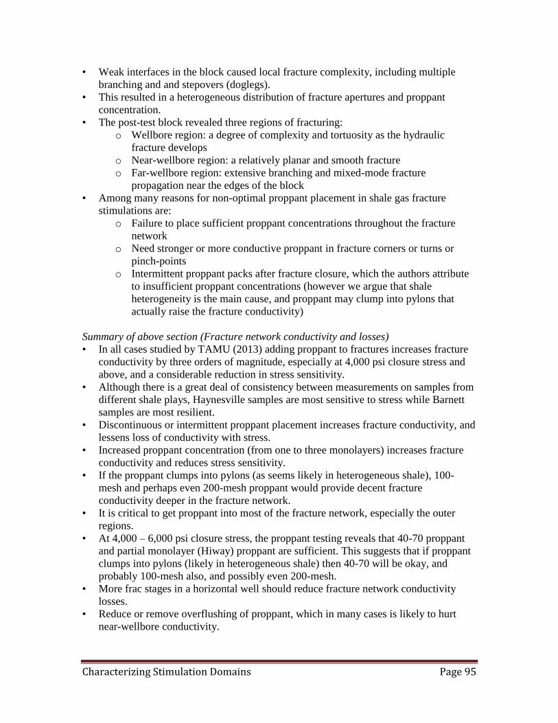
3.6 PROPPANT DESIGN STRATEGIES .............................................................. 96

4. CASE HISTORIES: WELL ANALYSES USING DOMANAL .......................... 111

4.1 INTRODUCTION ............................................................................................ 111

4.2 INJECTION PERMEABILITY AND CORRELATIONS ............................... 111

4.3 MULTIVARIATE REGRESSION FOR INJECTION PERMEABILITY ...... 120


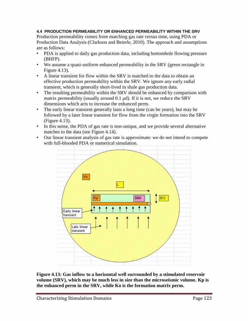
4.4 PRODUCTION PERMEABILITY OR ENHANCED PERMEABILITY

WITHIN THE SRV ................................................................................................ 123

4.5 LOSS OF INJECTION PERMEABILITY AFTER A WELL IS TURNED ON

TO PRODUCTION ................................................................................................ 132

4.6 CONCLUSIONS OF THIS SECTION ............................................................ 135

5. MAIN CONCLUSIONS OF PROJECT ................................................................. 137

NOMENCLATURE ................................................................................................... 142

ACKNOWLEDGEMENTS ........................................................................................ 144

REFERENCES CITED ............................................................................................... 145

APPENDIX A: ELEMENTS OF THE GEOMECHANICS MODEL ....................... 148

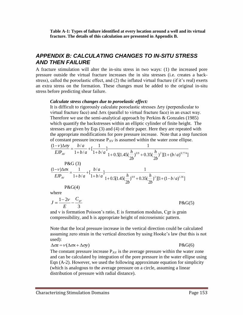
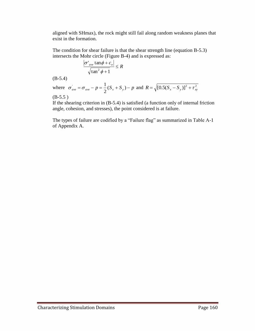
APPENDIX B: CALCULATING CHANGES TO IN-SITU STRESS AND THEN

FAILURE .................................................................................................................... 153

EXECUTIVE SUMMARY

Our method to characterize a stimulated reservoir is a two-step process. In the first step,

we match a microseismic (MS) pattern using a geomechanics model, which gives

injection permeability and porosity. Microseismic measurements provide qualitative

information about where a fracture stimulation goes. However, there is also quantitative

information, which has largely been neglected. We have developed a geomechanical

model to predict the extent of shear failure during fracture stimulation of a well. The

model identifies different types of failure, tensile and shear, which will occur on natural

fractures or vertical planes of weakness. By matching the model to the extent of the

microseismic cloud of shear failure, we obtain an injection permeability and porosity

which characterize the volume of the microseismic cloud.

From our modeling studies, a high injection permeability (tens or hundreds of md) is

required to pressure the formation and achieve failure out as far as the microseismic

events extend. Low injection porosity (< 0.1%) is required for the frac fluid to leak off

that far (this is much less than formation porosity of 3-5% typically). These numbers are

symptomatic of fracture-controlled flow during well stimulation. Reports on rapid

interference (‘pressure hits’) with offset wells support this interpretation. As a case

history, the method and results for sequential stimulation of two sister horizontal wells in

the Barnett shale are described.

In the second step we match gas rate versus time using PDA (Production Data Analysis),

which gives a much lower production permeability, and a stimulated reservoir volume

(SRV) size which is much reduced from the MS volume. Well and reservoir data from

five wells in the Fayetteville shale have been analyzed using new software called

DomAnal created under this project. The two perm-based diagnostics (injection and

production perm) have been correlated to various fracture treatment parameters, to try to

improve fracture stimulations.


Results and conclusions are:

• Potential horizontal fracture components in three wells may act to reduce breadth and

height of the MS cloud (ie, less outward and height spread of fracture fluid).

• The MS cloud for the shallowest well is smallest of all five wells for the same

injection volume. This may be due to lower effective stress (easier to open fractures)

or to opening of horizontal fractures.

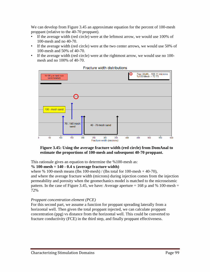
• Proppant volume is a very small fraction (<4%) of fracture network volume.

• Fracture spacing and fracture width tend to increase with effective stress (ie,

generally increasing depth) meaning created fractures are further apart and open

wider in deeper wells. This reflects the degree of consolidation/compaction of the

formation. This depth trend is consistent with fracture spacing from MS events in

other fields.

• Average fracture width in the network increases with depth which suggests to try an

increasing proportion of 40-70 sand with depth. In two wells in the Fayetteville, one

may even be able to use 30-50 sand.

• SRV productivity is a lot lower than MS injectivity (by 100 to 10,000 times) meaning

most of MS injectivity is lost after a well is turned on.

• The shallowest well is an outlier in that it retains more of the MS injectivity than

other wells.

• A regression equation enables a prediction of the SRV productivity. When effective

stress increases, SRV productivity decreases. This is expected: it is harder to create or

sustain a fracture network in a formation with larger effective stress.

• When amount of 40-70 proppant (or 100-mesh) increases, SRV productivity

increases. This is expected if proppant is needed to stop fractures in the network from

closing due to in-situ stress. But SRV productivity is more sensitive to 100-mesh than

to 40-70 proppant. This should mean that an increase in 100-mesh proppant will be

relatively more beneficial as compared with 40-70 proppant.

The two-part modeling adds insights previously unavailable. Our interpretation is based

on a quasi-uniform fracture network, with a system permeability enhancement, which

appears to be common in shales. The MS matching provides new information, via the

injection permeability and porosity, on spacing and aperture width of fractures in the

network. One way to retain more of the injection permeability, and the size of the SRV, is

to tailor the proppant to the width and spacing of the induced fracture network, to prop

more effectively the network of induced fractures.

At one level (called access level) we can compare average fracture aperture widths

against proppant sizes. These can be important for tailoring proppant size to access a

fracture network (eg, proppant mesh size that is too large cannot enter the fracture

network). For proppant that can enter the network, there is a second level (called spread

level), where the spreading of the proppant depends on the spacing and aperture width of

the network fractures, as well as the diameter and density of the proppant. All these

factors have been included in a conceptual model for proppant spreading away from a

horizontal well. This approach may help operators optimize proppant transport in shale

gas and oil wells, to retain a larger SRV (stimulated reservoir volume), and greater


permeability enhancement within the SRV (SRV sizes we find from transient analysis of

gas rates are much less than microseismic volumes).

Finally, our fracture widths are consistent with proppant sizes commonly used in the field

in shales, and this supports the geomechanics model used to match microseismic data to

determine the fracture widths.

1. MICROSEISMIC CLOUDS: MODELING AND IMPLICATIONS

1.1 INTRODUCTION

At present, information collected during well stimulations in tight shales is not fully

utilized. The microseismic patterns that are used in a qualitative way to judge the extent

of the stimulation, can also be analyzed quantitatively to determine during injection the

enhanced permeability in the fracture network. This requires a geomechanics model that

can predict shear failure and match the microseismic pattern (which is caused by shear

failure in the formation). In several cases where this has been done, it has been found that

the permeability is greatly enhanced during injection (ie, during stimulation).

An in-house semi-analytic screening model was developed in 2005, and the approach was

similar to earlier approaches (Warpinski et al, 2004). The model predicted the failure

extent away from a parent fracture, and was applied first to coalbed methane wells

(Palmer et al, 2005), and later to wells in the Barnett shale (Palmer et al, 2007). As pore

pressure diffuses away from a parent fracture plane, it induces shear failure in the

reservoir out to some distance which can be predicted from in-situ stresses and rock

strengths. The modeling requires a leakoff algorithm that calculates the pore pressure

distribution, as well as some sophisticated geomechanics such as poroelastic increases of

in-situ stresses, and prediction of shear failure. The model has been used to match the

microseismic patterns in several separate well stimulations (Palmer et al, 2009). The

injection permeability enhancements obtained from the matching appear to be consistent

with pressure-dependent leakoff values in tight gas plays, and are similarly attributed to

fracture-controlled permeability and porosity. The matching results were also consistent

with the properties (aperture width and spacing) of fracture networks.

Other geomechanics models have been developed to match a microseismic pattern.

Recent advances in complex fracture modeling have allowed a prediction of fracture

propagation in unconventional reservoirs (Xu et al, 2010; Meyer, 2009). At one extreme

are sophisticated models (Rahman et al, 2002; Weng et al, 2011), while other models are

less so (Xu et al, 2009; Cipolla et al, 2011). The model by Weng et al (called UFM)

argues that stress anisotropy, natural fractures, and interfacial friction play key roles in

creating a fracture network, and the results demonstrate the influence of rock fabric and

stress on fracture complexity. Future work will investigate fracture complexity using

higher viscosity frac fluids, different proppant sizes, and natural fractures that are oblique

to the horizontal stress. The Wire-mesh model of Cipolla et al (2011) is a semi-analytic

screening model, and several parametric studies have been investigated, including the

non-uniqueness of frac pressure matching, and reconciling the model pressures with those

in the field. Application of the model can provide surface area of the total fracture


network, as well as proppant distribution within the network. However for an input the

model requires independent data on natural fracture spacing.

Although our model was a screening model, it captured the keys to well stimulation in

unconventional plays, and the modeling results appeared to reflect the important physics.

More sophisticated models require more input parameters, and take a longer time to run.

One new aspect of the model was that the average fracture aperture width could be

obtained from the permeability during injection (Palmer and Moschovidis, 2010). This

offered the prospect of tailoring the proppant so that it would have better access to the

fracture network. In regard to proppant, decades have been spent trying to optimize

proppant design for single vertical fractures. Lab tests and theory have been the basis for

this. But for proppant transport in a fracture network, lab tests are difficult, and

theoretical predictions are much more challenging than for a single vertical fracture.

However, some learnings from a single vertical fracture with rough walls (e.g. proppant

fall rates, holdup, and bridging) may be applicable to a fracture network (Liu et al, 2006;

Barree and Conway, 2001). The UFM model by Weng et al (2011) implements 1D fluid

flow and proppant transport in the fracture network, using assumptions similar to those

for pseudo-3D fracture models. Proppant transport for slickwater frac fluids consists of a

proppant bank at the bottom of the fracture, a slurry layer in the middle, and clean fluid at

the top, for each element of the fracture network. Modeling results reveal that only a

small fraction (2-5%) of the induced fracture network is occupied by proppant. The

reasons are rapid proppant settling, and proppant bridging in the side fractures which

have small aperture width. Cipolla et al (2010) have argued in this case that only the

propped area contributes to production, although this must depend on the permeability of

natural fractures that have been sheared and dilated during the frac stimulation, and

remain open due to asperity mis-matches after a well is brought online (Palmer and

Moschovidis, 2010).

In summary, modeling of fracture networks (ie, complex fracturing and proppant

transport) is evolving rapidly, and our disclaimer is that the above is not meant to be a

comprehensive review.

1.2 MODELING SHEAR FAILURE DURING INJECTION (GEOMECHANICAL MODEL)

Approach:

The approach has been discussed elsewhere (Palmer et al, 2007; Palmer and

Moschovidis, 2010), and we offer only a summary here. We model shear failure over a

region illustrated by the microseismic pattern of Figure 1.1. The figure happens to

represent a vertical well, but this discussion also applies to a horizontal well. The

microseismic events, which indicate shear failure, are usually caused by elevated pore

pressure in the formation. So we first have to model how pore pressure is transmitted

outwards from the well during a frac stimulation. This is accomplished by assuming a

vertical fracture quickly extends the length of the long azimuth of the microseismic

pattern (not quite the full length, but a large fraction of this, depending on the

length/breadth aspect of the microseismic pattern. This “virtual” fracture (with

bottomhole pressure Pf) is an artifice to act as the source of elevated pore pressure which

spreads outwards in an elliptical pattern, governed by the leakoff rate and in particular the

injection porosity and permeability.


Figure 1.1: Frac water spreading killed five wells in Barnett Shale (Fisher et al,

2002). The orange square on the left is the observation well which detects the

microseismic bursts.

This model is simplistic, in that the spreading of pore pressure from a well may be much

more complicated. In many shale plays, for example, there may not be a single dominant

vertical fracture. But in some cases there will be, and to model the elliptical spreading of

pore pressure from a line pressure source is probably a good approximation in many

cases (Koning, 1985, 1988). Once the pore pressure distribution is modeled, we can use

this along with in-situ stresses and a failure surface, to predict the zone of shear failure.

Actually, in the model the in-situ stresses are modified by two things: (1) the poroelastic

backstress, and (2) the presence of the vertical source fracture, if it’s a real fracture

(Koning, 1985, 1988). We can use this model to match a microseismic pattern around a

well (which reflects the zone of shear failure), in which case the matching parameters are

injection porosity and permeability (the permeability will be the perm to frac fluid, which

should be close to the absolute permeability).

Other model assumptions are:

Our view is that microseismic events are associated with pressure-induced shear

slip on fractures or planes of weakness which are vertical (Warpinski, private

comm., 2009). An alternate suggestion is that strain-induced shear slip occurs on

weak bedding planes, perhaps ones which have significantly different moduli on

each side of the plane. This would traverse a formation rapidly, since a stress

wave induced by a growing fracture would travel at the speed of sound (Barree,

private comm., 2012).


The fracture has a constant height (which can be different from the reservoir

thickness), and propagates under a constant fracture pressure.

The fluid leak-off rate is equal to the injection rate. That is, if a virtual fracture

exists, the rate of change of its volume is small compared to the injection rate.

The failure front is closely associated with the water front.

Water front versus failure front:

Slickwater fracs are of most interest in this paper, because they cause the widest spread of

microseismic events compared with other frac fluids. The clearest indication that the

failure front (microseismic front) is associated with the water front comes from Figure

1.1, where the wells killed by frac-water influx are close to the perimeter of the

microseismic pattern. Although wells 1 and 2 lie outside the microseismic pattern, this

may be due to the attenuation limit of the microseismic signals traveling to the

observation well. This association was also the position taken by Warpinski et al (2004).

Figure 1.2: Leakoff pressure profile with distance from main fracture face. The

assumption is that the failure front is the same as the water front. Ki is the injection

permeability. The total leakoff-driven pressure drop is Pf – Pi = dP1 + dP2.

The pressure profile driven by leakoff from the virtual fracture is the remaining issue. At

one extreme, Warpinski et al (2004) has argued that the pressure at the water front is Pi,

the initial reservoir pressure. This assumes an evacuated reservoir, and is the basis for the

standard leakoff treatment (ie, viscosity-dominated leakoff). However, the reservoir is not

evacuated, but is filled with gas, and the pressure drop in the gas zone (dP1 in Figure 1.2)

may be substantial. Basically this is because the mobility of the gas in the gas zone


(Ko/µo) can be much smaller than the water in the water zone (Kw/µw), meaning more

resistance to the movement of gas ahead of the waterfront (the ultra-small virgin perm Ko

is the determining factor in this comparison). This factor also implies that the gas zone of

rapid pressure falloff is limited generally to a few tens of feet at most.

Figure 1.3: Two different pressure profiles in the water zone. Blue dashed line is

Warpinski approximation with low Ki. Red line is high Ki scenario. Because shear

failure depends on many factors, this figure is just a schematic to illustrate how

shear failure extends further out when pressure in the formation is higher.

We do not have a model for calculating dP1, due to several physical uncertainties not

discussed here, and we decided to make dP1 an input parameter. At one extreme dP1 = 0,

and this is the Warpinski approach shown in Figures 1.2 and 1.3. At another extreme dP1

can be high, such as 0.95 of the total pressure drop (Pf-Pi). The pressure profile in the

water zone determines the shear failure extent (Figure 1.3). If Pfail is the pressure at

which shear failure occurs, as calculated by the Mohr-Coulomb failure criterion, failure

for the blue line may occur far from the water front. To correct this, dP1 is raised toward

the red line, until failure occurs near the water front (and matches the microseismic

spread). The choice of dP1 has implications for the injection permeability Ki, and in fact

we calculate the injection permeability from an equation for the leakoff of frac fluid from

the virtual fracture. If dP1 = 0, we have the situation in Figure 1.2, and Ki will be a lower

limit. On the other hand, if dP1 = 0.95 (Pf-Pi), this will result in a high value for Ki

(perhaps an upper limit).

Geomechanics model: The details of the geomechanics model are described in Appendix A.

Choosing orientation of virtual frac:

The virtual frac is the (artificial) source of elevated pore pressure, which spreads

outwards in a 2D elliptical pattern (Koning, 1985, 1988), and which will cause the shear


failure that manifests as microseismic events. As such, the orientation of the virtual frac

should be related to the in-situ stresses, while its length comes from the length/breadth of

the microseoismic pattern as described earlier.

For a vertical well, such as in Figure 1.1, the long axis of the microseismic pattern is

oriented north-east, and this would be the oriention of the virtual frac. For a horizontal

well, there are two possible situations:

(1) Well aligned with SH, the maximum horizontal stress. In this case, the virtual frac

should be along SH also, ie, a longitudinal frac, as illustrated by Figure 1.4.

(2) Well aligned with Sh, the minimum horizontal stress, which is the usual situation in

shale gas plays. In this case, there can be many separate frac stages, typically spaced

about 300 ft along the length of the well. Within each frac stage are usually 4-6

perforation clusters, which may therefore induce 4-6 transverse fractures, spaced 50-

75 ft apart (or there could be fewer fractures). Whether these dominant transverse

fractures exist or not is controversial, and this leads to two more situations:

a. If there is evidence for discrete transverse fractures, then each of these

fractures could act as a virtual fracture in sourcing the enhanced pore pressure.

This would require matching of the microseismic pattern formed during each

individual frac stage, and would be a challenging task needing high-resolution

data.

b. If there is no evidence for discrete transverse fractures (eg, frac pressure rising

and evenly-spread microseismic events), then the horizontal well itself can be

regarded as a virtual fracture source for the 2D pressure spreading into the

formation. This case is illustrated by Figure 1.5. However, in this case we do

not calculate stress changes due to an inflated virtual fracture, because we see

no evidence for an actual longitudinal fracture.


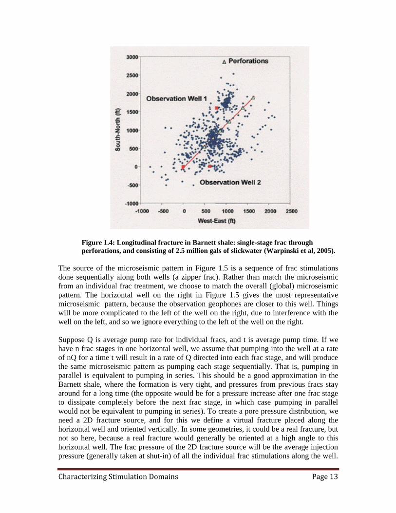
Figure 1.4: Longitudinal fracture in Barnett shale: single-stage frac through

perforations, and consisting of 2.5 million gals of slickwater (Warpinski et al, 2005).

The source of the microseismic pattern in Figure 1.5 is a sequence of frac stimulations

done sequentially along both wells (a zipper frac). Rather than match the microseismic

from an individual frac treatment, we choose to match the overall (global) microseismic

pattern. The horizontal well on the right in Figure 1.5 gives the most representative

microseismic pattern, because the observation geophones are closer to this well. Things

will be more complicated to the left of the well on the right, due to interference with the

well on the left, and so we ignore everything to the left of the well on the right.

Suppose Q is average pump rate for individual fracs, and t is average pump time. If we

have n frac stages in one horizontal well, we assume that pumping into the well at a rate

of nQ for a time t will result in a rate of Q directed into each frac stage, and will produce

the same microseismic pattern as pumping each stage sequentially. That is, pumping in

parallel is equivalent to pumping in series. This should be a good approximation in the

Barnett shale, where the formation is very tight, and pressures from previous fracs stay

around for a long time (the opposite would be for a pressure increase after one frac stage

to dissipate completely before the next frac stage, in which case pumping in parallel

would not be equivalent to pumping in series). To create a pore pressure distribution, we

need a 2D fracture source, and for this we define a virtual fracture placed along the

horizontal well and oriented vertically. In some geometries, it could be a real fracture, but

not so here, because a real fracture would generally be oriented at a high angle to this

horizontal well. The frac pressure of the 2D fracture source will be the average injection

pressure (generally taken at shut-in) of all the individual frac stimulations along the well.


Pumping into the virtual fracture at a rate of nQ for a time t, along with the 2D

pressure/leakoff model, will ensure that (approximately):

• Frac fluid will penetrate the same distance into the formation as in each separate

frac stage (injection porosity φi is calculated from this)

• The same pressure profile occurs away from the well as for each separate frac

stage (injection permeability Ki is calculated from this)

Figure 1.5: Multi-stage sequential fracs through two wells in Barnett shale (King et

al, 2008). Each color is the microseismic spread from a single set of perfs in one

well.Typical length: breadth aspect ratio of the individual microseismic

distributions is ~0.5 (ie, the spread is broader than its length). The ellipse is centered

on the well on the right, and encompasses most of the microiseismic events to the

right of this well.

Also, our approach and model should apply whether the microseismic distribution in each

frac stage is uniform, or discrete as in a single vertical fracture:

• If uniform, the injection permeability Ki will be interpreted as a widespread perm

enhancement due to a fracture network (the microseismic distribution of this

paper belongs here). And for this extreme we can ask how to tailor the proppant to

maximize the conductivity of the fracture network (this is new). This scenario is

the emphasis of this paper.

• If discrete, Ki will be interpreted as a perm enhancement largely due to one (or

more) discrete vertical fractures, plus possibly some minor contribution from a

surrounding fracture network. In this case, we will have contributions to the

produced gas from discrete propped fractures, as well as a surrounding network of

smaller fractures. If the fracture network is ignored, we can bring to bear 40 years

of proppant design in single vertical fractures.


The degree of leakoff from a fracture network into the shale matrix can affect the

injection porosity, but not the permeability. Initially we assumed this leakoff was

negligible, but it may not be if the network fractures are closely spaced. We have chosen

a fracture fluid efficiency of 81% to illustrate the results below. If the efficiency were

lower (ie, more fluid loss from the fracture network), the injection porosity would be

lower, but injection permeability would stay the same in our model. This in turn implies

that fracture spacing and aperture width would be larger. It has been suggested that fluid

efficiency in a fracture network may be as low as 50%, even in tight shales (Weng,

2012).

There is an additional complication. Our model assumes the virtual frac is aligned with

SH. However, in Figure 1.5 the virtual frac is placed along the well on the right, since

this is properly the source of pressure for that well. However, this is not aligned with SH:

it is about 60 deg off. This requires a correction, including a switch of the stresses, which

we have not addressed yet (although it’s a correction which will not alter the conclusions

of this paper). 1.3 MATCHING MICROSEISMIC CLOUDS: CASE STUDY

In the well of Figure 1.5, the input parameters for the geomechanics model are shown by

Table 1.2. These parameters are typical of the Barnett shale in Western Parker county.

Because no measurements were made of in-situ stress or bottomhole frac pressure here,

we have inferred these from vertical depth (~5000 ft) and ISIPs at the end of slickwater

fracs in Parker county (King, 2011):

• 4700-4950 ft depth to top of Barnett shale in Parker county

• Final ISIPs taken from many frac profiles range 1000-1400 psi

• ISIP = 1400 psi is consistent with D = 5500 ft, and Sh = 0.65 psi/ft and implies Pf

= 3875 psi

• ISIP = 1000 psi is only consistent with D = 5000 ft, and Sh = 0.60 psi/ft and

implies Pf = 3650 psi

So either of these scenarios might apply to the sequential fracs in the well of Figure 1.5

(we have modeled both scenarios).

In the first matching trials below, we choose D = 5500 ft, and Sh = 0.65 psi/ft which

implies Pf = 3875 psi. Since the two horizontal stresses Sh and SH cannot be much

different (e.g., see the microseismic spreads in Figures 1.1 and 1.4), we choose SH = 0.75

psi/ft. The various matches we obtained are given in Figures 1.6-1.9 below. Note that Cfr

is a fraction between 0 and 1 which defines the amount of pressure drop from the

horizontal well pressure source to the edge of the frac water zone (eg, Cfr = 1 implies no

pressure drop, while Cfr = 0 means frac pressure at wellbore drops to initial reservoir

pressure at the edge of the water zone).


Table 1.1: Input parameters for the geomechanics model to match the microseismic

pattern, and calculate injection porosity and permeability.

Figure 1.6: Geomechanics model which does not match microseismic ellipse in

Figure 1.5: Sh = 3575 psi, Pf = 3875 psi, weak plane angle = 0 up to 35⁰, eff = 81%,

Cfr = 0.99, φi = 0.019%, Ki = 3837 md. We cannot match the microseismic pattern if

weak planes are oriented at < 35⁰ to Shmin.

Depth = 5500 ft 5000 alternate

Frac injection time = 3 hrs av for single-stage

Frac pump rate = 8 x 35 = 280 bpm (8 frac stages, and average pump rate is 39 bpm)

Semi major axis = 3050/2 = 1525 ft

Semi-minor axis = 1850/2 = 925 ft

Swo = 0.3

Gas SG = 0.7

Res temp = 160F

Friction angle = 31 deg

MS height = 380 ft (average)

Inj fluid viscosity = 1 cp (slickwater)

Pi = 2860 psi (from 0.52 psi/ft x 5500 ft) 2600 alternate

Pf = 3875 psi 3650 alternate

E = 5e6 psi

v = 0.24

SHmax = 0.75 psi/ft x 5500 = 4125 psi 0.70 x 5000 = 3500

Shmin = 0.65 psi/ft x 5500 = 3575 psi 0.60 x 5000 = 3000 alternate

Cohesion = 100 psi (for fractured formation)

Tensile strength = 30 psi (~cohesion/3)

Fabric angle = 0 (weak fabric planes should be aligned with stresses)


Figure 1.7: Geomechanics model to match microseismic ellipse in Figure 1.5: Sh =

3575 psi, Pf = 3875 psi, weak plane angle = 40⁰, eff = 81%, Cfr = 0.99, φi = 0.019%,

Ki = 12,791 md. For this high Cfr and Ki, we can match the microseismic pattern

but only if there are weak planes at 40-45⁰ to the stress direction.



Ki = 1279 md. For 45⁰ weak planes, this gives the minimum Cfr and Ki to match the

microseismic pattern.

Summary for D = 5500 ft and Sh = 0.65 psi/ft:

• We assumed a fracture fluid efficiency of 81%, which accounts for leakoff from

the fracture network into the tight shale matrix. This lowers the injection porosity

from its value using 100% efficiency.

• We cannot match the microseismic pattern using weak planes oriented < 40 deg

from Sh (Figure 1.6), but we can get a match using > 40 deg (Figure 1.7). For an

angle of 45 deg, Ki = 1279 md is required to match the microseismic pattern


(Figure 1.8).

• We can also match the microseismic pattern using randomly-oriented weak

planes, but only if Ki = 1279 md (Figure 1.9).

• Using the initial set of input parameters, we cannot match the microseismic

pattern using the conventional picture of two perpendicular sets of fractures

aligned with SH and Sh (Figure 1.10)

• Maybe there exists a third set of vertical fractures or weak planes lying between

the two main sets (as suggested in Figure 1.10). This would be equivalent to a

random set of weak planes, and would induce shear failure to match the

microseismic pattern if Ki = 1279 md. So a third set of fractures, or randomly-

oriented weak planes, is the only way we can match the microseismic pattern,

provided Ki = 1279 md.

• When injecting into a formation and opening a network of fractures, the pore

pressure distribution develops so as to minimize the energy (ie, work against the

in-situ stresses). This leads to the minimum pressure at the failure (and water)

front that would accommodate the injected flow and induce shear failure that

extends to the water front. Consequently the minimum Cfr that extends the shear

failure to the microseismic boundary should be selected. Cfr values greater than

this would extend failure beyond the water front, although we are not modeling

shear failure in this generally small region.


3575 psi, Pf = 3875 psi, weak planes are random, eff = 81%, Cfr = 0.90, φi = 0.019%,

Ki = 1279 md. For random weak planes, this gives the minimum Cfr and Ki to

match the microseismic pattern.


Figure 1.10: Primary fracture direction (red) at roughly N45⁰E, secondary (blue) at

S 45⁰E plane (King et al, 2008). Up to three fracture directions have been recorded.

Alternate depth and stress in Parker County:

In the second set of matching trials below, we choose D = 5000 ft, and Sh = 0.60 psi/ft

which implies Pf = 3650 psi. Since the two horizontal stresses Sh and SH cannot be much

different (eg, see the microseismic spreads in Figures 1.1 and 1.4), we choose in this case

SH = 0.70 psi/ft. The various matches we obtained are given in Figures 1.11-1.13.

Summary for D = 5000 ft and Sh = 0.60 psi/ft:

• We assumed a fracture fluid efficiency of 81%, which accounts for leakoff from

the fracture network into the tight shale matrix. This lowers the injection porosity

from its value using 100% efficiency.

• We cannot match the microseismic pattern using weak planes at < 20 deg from

Sh.

• We can match the microseismic pattern using weak planes at 20 deg from Sh, but

Ki = 2473 md is required (Figure 1.11).

• We can match the microseismic pattern using weak planes at 25 deg from Sh, but

Ki = 824 md is required (Figure 1.12).

• We can match the microseismic pattern using randomly oriented weak planes, if

Ki = 225 md (Figure 1.13).

• Using this alternate set of input parameters, we can match the microseismic

pattern using the conventional picture of two perpendicular sets of fractures

aligned with SH and Sh (Figure 1.10), but only if there is local variability by 20

deg in natural fracture or stress orientation, and provided Ki = 2473 md.

• An alternative is a third set of fractures or weak planes at ~45 deg to the two main

sets (as suggested in Figure 1.10). This situation approximates weak planes that

are randomly oriented, and would induce shear failure to match the microseismic

pattern if Ki = 225 md. So a third set of fractures, or randomly-oriented weak

planes, is the other way we can match the microseismic pattern, provided Ki =

225 md.

• Based on these two geometry scenarios, the modeling suggests the injection

permeability has to be at least 225 md, but may be ten times higher, up to 2473

md.










In the alternate depth scenario, a consequence of the shallower depth and lower stress is

that the net fracture pressure is higher (650 psi versus 300 psi for the first depth scenario).

We note that both of these pressures fall within Coulter’s range of 100-900 psi (Coulter et

al, 2004). A higher pore pressure (and therefore net fracture pressure) is the most critical

parameter for shear failure, and that is why the alternate depth scenario predicts more

shear failure at lower weak plane angles (eg, 20 or 25⁰). A higher net fracture pressure is

also consistent with proppant slugs that were used deliberately to create a more complex


fracture, slow the outwards fracture propagation, and increase the fracture pressure, as

was done in this sequential frac operation (King et al, 2008). A higher net fracture

pressure could also explain the high density of microseismic events in these two wells

(see Figure 1.5).


3000 psi, Pf = 3650 psi, weak planes are random, eff = 81%, Cfr = 0.45, φi = 0.019%,

Ki = 225 md. For random weak planes, this gives the minimum Cfr and Ki to match

the microseismic pattern.

1.4 CHARACTERIZING THE FRACTURE NETWORK OR SRV

In the region of the microseismic cloud of Figure 1.5, which is associated with complex

fracturing and a fracture network (King et al, 2008), the injection permeabilities from our

modeling are relatively high (> 225 md), and the injection porosity is low (0.019%). For

a quasi-uniform fracture network, these represent fracture-controlled injection (Palmer

and Moschovidis, 2010). The low porosity is required for the frac fluid to leak off as far

as the perimeter of the microseismic cloud. The high injection permeability is required to

diffuse pressure and achieve shear failure out as far as the microiseismic events extend

(see also Warpinski et al, 2009). The distribution of the five offset wells in Figure 1.1 that

were killed by frac fluid supports this picture, as discussed by Warpinski et al (2009).

This interpretation is also supported by other reports of rapid interference seen at offset

wells during frac stimulations of long horizontal wells.

This relatively high injection permeability is the bulk permeability of the SRV, during

well stimulation and before the well is turned on to production. It includes the

permeability of the fractures in a network (see Figure 1.1) combined with virgin

permeability in between fractures. The network permeability usually dominates because

shale plays are very tight (< 1 µ). If in the network we assume two sets of vertical

fractures, for example, we can calculate average fracture spacing and aperture width from

φi and Ki using relationships like those in Figure A-2 (although that figure is for one set


of fractures only). This information may be important for choosing proppant type, size,

and concentration for optimal fracture treatments in tight shales.

One or two sets of vertical fractures, assumed to have constant aperture width and

spacing, gives a unique fracture porosity and permeability (Reiss, 1980). This is true only

if we ignore tortuosity of gas flow in the fractures, which will reduce the fracture

permeability. We have not corrected for this, as we assume the effect is relatively small

for gas flow. For two fracture sets the equations can be inverted to give:

Fracture aperture width b = √(2.4Ki/ϕi) and fracture spacing a = 2b/(100ϕi), with ϕi in %,

Ki in md, b in microns, a in cm. Using from our modeling results φi = 0.019% and Ki =

225 md (Figure 1.13) gives b = 169 µ and a = 177 cm (5.8 ft). This average fracture

spacing is much less than other fracture spacing ranges inferred from microseismic data

(i.e., planes of simultaneous bursts):

50–200 ft in Barnett shale (Fisher et al, 2002)

60-80 ft average in Barnett shale (see Figure 1.10)

16-130 ft in Cadomin (Kovalsky, 2007).

From our modeling, a possible upper limit for Ki is 2473 md (Figure 1.11), in which case

the injection permeability if weak planes and stresses are offset by ~20⁰. This would give

a = 588 cm or 19.3 ft. This fracture spacing, which is still relatively small, suggests that

measurements like Figures 1.1 and 1.10 are revealing only the largest microseismic

events. This makes sense because the largest events would occur due to shear failure on

the longer fractures (or weak planes), and these would be spaced further apart (because

natural fracture lengths and spacings are fractal).

The average aperture width of b = 169 µ comes from Ki = 225 md. The possible upper

limit of 2473 md would give 559 µ. This range of 169 – 559 µ can be compared with

typical proppant sizes used in shale-gas frac treatments in Figure 1.14. An obvious

conclusion is that 40-70 mesh proppant will not fit into network fractures at the smaller

end, while 100-mesh proppant would have much better access. Note that these aperture

width calculations are average widths: in a real shale reservoir there will be a spread of

aperture widths around each average number.

Figure 1.14: Range of aperture widths (169 – 559 µ) inferred from range of injection

permeabilities obtained by matching the microseismic pattern in Figure 1.5. The


reference fracture widths of 10-100 µ are for unstimulated natural fractures (Reiss,

1980).

There are uncertainties in our modeling and matching of the Parker county frac

stimulations:

Cfr is a parameter that is varied to achieve a match of the microseismic pattern.

However it might be possible to derive Cfr by separate modeling of the pressure

at the moving water front (a complicated problem), and this would add an extra

constraint on the matching.

The injection permeability depends on the failure envelope chosen for a fractured

shale formation which contains natural fractures or planes of weakness: in this

paper we have assumed reasonable values for cohesion of 100 psi and for friction

angle of 31⁰ and we have not varied these.

The maximum horizontal stress Shmax: we assumed in both scenarios of the

Parker county case study that this was higher than Shmin by 0.1 psi/ft.

The viscosity of the slickwater that leaks off into the fracture network. While

water viscosity may be 0.3 cp under static bottomhole temperature, the actual

fluid would be warmer due to the high pump rate. The additives used in

slickwater for friction reduction also increase viscosity, as well as the wall

roughness in the fracture (Weng, 2012). We used 1 cp, but note that the injection

permeability is proportional to the viscosity, so it’s quite a strong effect.

1.5 HOW IMPORTANT IS A FRACTURE NETWORK AND ITS CONDUCTIVITY?

The desirability of a fracture network has been espoused by King et al (2008), because

cracking more of the rock will allow the gas in a shale (which is usually very tight) easier

access to the fractures in the network, and therefore to the wellbore. Different ways to

create a fracture network are discussed in that paper. In the Barnett shale, one well’s gas

recovery was nicely matched by a model which assumes only a fracture network (i.e., no

dominant vertical fractures), and appears to confirm this picture (Figure 1.15). Another

case is in the Bakken shale, where fracture designs by one operator use only slickwater as

frac fluid to induce a wider spread of microseismic events, and a higher oil rate, than in

offset wells treated by a hybrid frac design (Pearson, 2011). This result runs counter to

current thinking about the need for higher fracture conductivities in tight shale-oil plays.

Our method to characterize a stimulated reservoir volume (SRV) is actually a two-step

process. In the first step, as described in this paper, we match a microseismic pattern

using a geomechanics model, which gives injection permeability and porosity. In the

second step we match gas rate versus time from the same well using PDA (Production

Data Analysis), which gives a production permeability. We have found previously that

most of the injection permeability is lost when a well is turned on, and ways to retain

more of the injection permeability have been suggested (Palmer and Moschovidis, 2010).

One of these ways is to tailor the proppant to the width and spacing of the induced

fracture network, to prop more effectively the network of induced fractures.

As shown by Figure 1.15, an increase in fracture conductivity from 2 to 5 md-ft would

increase the cum gas recovery by 30-50%, which is huge for a well making >1 mmcfd.

Note however that fracture spacing is 100 ft in the network of Figure 1.15, and if this


spacing were smaller, say 50 ft or 25 ft, or even 10 ft, the cum gas would be larger still

(Mayerhofer, 2007).

Figure 1.15: Cum gas recovery from a horizontal well matched to a fracture

network model (adapted from Cipolla, 2009). Also shown are two extremes of

fracture geometry: high-conductivity discrete fractures versus low-conductivity

fracture network.

The concept of a model to tailor proppant to a fracture network is displayed in Table 1.3.

Although the importance of proppant has been controversial, the lab results of Fredd

(2001) make it clear that the conductivity of a partially-propped fracture can be vastly

greater than an unpropped fracture, even if the unpropped fracture is rugose (Palmer and

Moschovidis, 2010). A model like Table 1.3, but expanded, is planned to offer a basis for

choosing alternative proppants for shale frac treatments. Note that the proppant is

assumed to be partially-propped (rather than in a proppant pack), which is likely in a

complex fracture (Cipolla et al, 2008). Also, we have not included the effect of

embedment in Table 1.3.


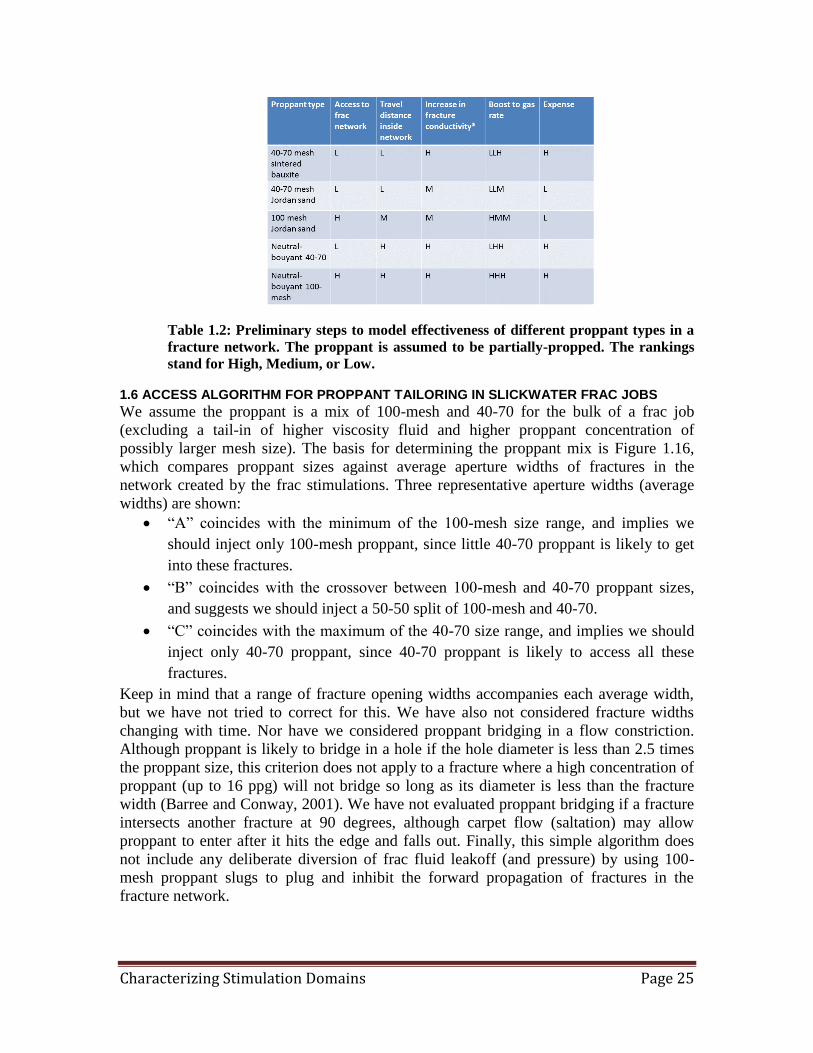
Table 1.2: Preliminary steps to model effectiveness of different proppant types in a

fracture network. The proppant is assumed to be partially-propped. The rankings

stand for High, Medium, or Low. 1.6 ACCESS ALGORITHM FOR PROPPANT TAILORING IN SLICKWATER FRAC JOBS

We assume the proppant is a mix of 100-mesh and 40-70 for the bulk of a frac job

(excluding a tail-in of higher viscosity fluid and higher proppant concentration of

possibly larger mesh size). The basis for determining the proppant mix is Figure 1.16,

which compares proppant sizes against average aperture widths of fractures in the

network created by the frac stimulations. Three representative aperture widths (average

widths) are shown:

“A” coincides with the minimum of the 100-mesh size range, and implies we

should inject only 100-mesh proppant, since little 40-70 proppant is likely to get

into these fractures.

“B” coincides with the crossover between 100-mesh and 40-70 proppant sizes,

and suggests we should inject a 50-50 split of 100-mesh and 40-70.

“C” coincides with the maximum of the 40-70 size range, and implies we should

inject only 40-70 proppant, since 40-70 proppant is likely to access all these

fractures.

Keep in mind that a range of fracture opening widths accompanies each average width,

but we have not tried to correct for this. We have also not considered fracture widths

changing with time. Nor have we considered proppant bridging in a flow constriction.

Although proppant is likely to bridge in a hole if the hole diameter is less than 2.5 times

the proppant size, this criterion does not apply to a fracture where a high concentration of

proppant (up to 16 ppg) will not bridge so long as its diameter is less than the fracture

width (Barree and Conway, 2001). We have not evaluated proppant bridging if a fracture

intersects another fracture at 90 degrees, although carpet flow (saltation) may allow

proppant to enter after it hits the edge and falls out. Finally, this simple algorithm does

not include any deliberate diversion of frac fluid leakoff (and pressure) by using 100-

mesh proppant slugs to plug and inhibit the forward propagation of fractures in the

fracture network.


The A, B, and C assignments above lead to an equation to select the percentage of

proppant in the 100-mesh and 40-70 mix:

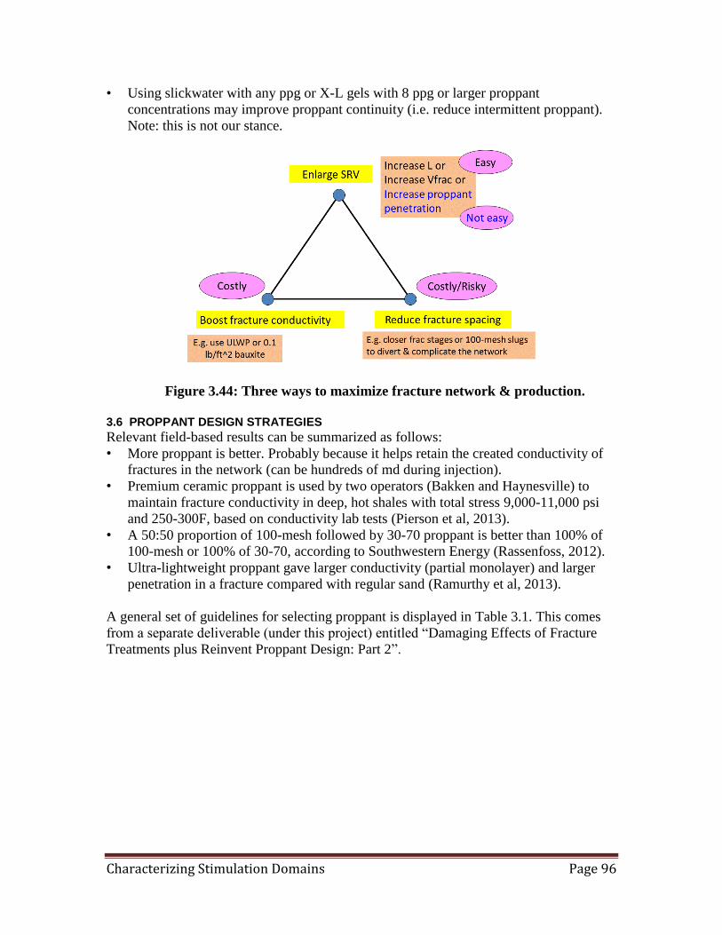
% 100-mesh = 140 – 0.4 x (average fracture width)

where % means (lbs 100-mesh) / (lbs total for 100-mesh + 40-70) and average fracture

width (microns) during injection comes from injection permeability and porosity when

the geomechanics model is matched to the microseismic pattern. If the equation gives a

negative % for an average fracture width near or above 350 µ, it simply means use 100%

of the 40-70 proppant (and perhaps some 30-50 proppant) because all the 40-70 proppant

should have access to the fracture network. Similarly, if the equation gives > 100% for an

average fracture width below about 100 µ, it simply means use 100 % of 100-mesh

proppant (or maybe use some 200-mesh) because none of the 40-70 proppant should have

access to the fracture network.

Figure 1.16: Basis for algorithm to select proppant mix based on average aperture

width of fractures during injection, and proppant grain sizes.

For comparison, some current usages of 100-mesh proppant in the field are:

1. Almost 100% of 100-mesh sand was used in one frac job in a tight sand in

Canada, and the gas rate was just as good as a mix of 100-mesh and 40-70 used in

many jobs previously (this may suggest 100-mesh sand got into more fractures).

2. Barnett: 2-3 years ago operators were moving to more 100-mesh.

3. Fayettville: 50% of 100-mesh is used by one operator in areas of gas production,

based upon several well trials (Rassenfoss, 2012).

4. Horn River: 50% of 100-mesh is used by one operator.

As far as we know, these proppant proportions have only been determined empirically

(i.e., by trial and error in the field, which is expensive), and an analysis like Figure 1.16

may be beneficial in increasing production from shale-gas plays.

In the likely context of an irregular fracture network, the complexities of proppant access

and transport make this a formidable problem to solve. Nevertheless, we anticipate that

one consequence will be proppant clumping, or proppant “pylons”, which may be quite


effective in doing what proppant is supposed to do: hold open the network fractures

against pressure depletion. As an example, Barree and Conway (2001) have discussed the

formation of proppant nodes and proppant holdup in a main fracture that has leakoff sites

at discrete fissures. Cipolla (2009) has drawn pictures of proppant that falls out but

“catches” or bridges at fracture discontinuities. In our view, the potential exists for

improving production by getting more proppant into the induced fracture network.

Finally, this study raises the question of whether, in reality, proppant can get into

fractures induced by shear slip (the ones that give rise to the microseismic events). It

turns out that shear slip also opens fractures, and increases their porosity and

permeability. This is clear from the work of Olsson and Barton (2011), where shear slip

on granite samples has been carefully measured, along with fracture aperture widths (eg,

see their Figure 1.14). For a joint roughness coefficient of 5, mechanical aperture widths

span the range of 100-400 µ as shearing progresses. For a joint roughness coefficient of

10, the range is 400-1400 µ. These ranges actually encompass the spread of 169 – 559 µ

that we obtained in Figure 1.14. In the granite lab measurements the normal stresses

acting on the slip surface are <480 psi, which stress is not much different from the normal

stress in the alternative depth and stress scenario for the Parker county modeling above.

Depending on the joint roughness coefficient, it appears that fracture widths induced by

shear slip in shales should be large enough to enable proppant access, at least to some

degree. 1.7 CONCLUSIONS OF THIS SECTION

1. By matching (quantitatively) the geomechanics model to the microseismic cloud of

shear failure, we obtain an injection permeability and porosity, which characterize the

stimulated reservoir volume (SRV).

2. The geomechanics model is a “screening model” meaning point-by-point (ie, local

versus global) details of the natural fracture distribution, fluid leakoff, and failure

prediction are ignored.

3. The model can be applied to any formation in which microseismic data demonstrates

a spread away from the expected main fracture plane, as happens in many tight

shales. A number of different geometries have been modeled: horizontal vs vertical

wells, and transverse vs longitudinal fractures.

4. The geomechanics model has been applied to a case study of multi-stage sequential

fracs installed in a couplet of parallel wells in the Barnett shale. For D = 5500 ft and

Sh = 0.65 psi/ft, we cannot match the microseismic pattern using the conventional

picture of two perpendicular sets of fractures aligned with SH and Sh; a third set of

fractures, or randomly-oriented weak planes, is the only way we can match the

microseismic pattern, and provided Ki = 1279 md. For D = 5000 ft and Sh = 0.60

psi/ft, we can match the microseismic pattern using the conventional picture of two

perpendicular sets of fractures aligned with SH and Sh, but only if there is local

variability by 20 deg in natural fracture or stress orientation, and provided Ki = 2473

md. A third set of fractures, or randomly-oriented weak planes, is the other way we

can match the microseismic pattern, and provided Ki = 225 md. Based on these two

scenarios, the modeling suggests the injection permeability has to at least be 225 md,

but may be ten times higher, up to 2473 md.

5. The injection permeabilities from our modeling are relatively high (> 225 md), and


the injection porosity is low (0.019%). For a quasi-uniform fracture network, these

represent fracture-controlled injection. The low porosity is required for the frac fluid

to leak off as far as the perimeter of the microseismic cloud. The high injection

permeability is required to diffuse pressure and achieve shear failure out as far as the

microseismic pattern extends.

6. The results from the case study imply a fracture spacing of 5.8 – 19.3 ft. This is much

less than fracture spacing inferred from microseismic data, suggesting that detectable

microseismic events are due to shear failure on longer fractures (or weak planes)

which would be spaced further apart.

7. The results also imply an average aperture width in the range 169 – 559 µ, and that

100-mesh proppant would have better access than 40-70 mesh proppant to the low

end of the network fractures.

8. The concept of a method to tailor proppant to a fracture network is initiated. A

primitive algorithm for proppant tailoring in slickwater frac jobs is presented, based

on average fracture aperture width during injection, and this algorithm selects the

percentage of proppant in the 100-mesh and 40-70 mix. Previously, these proppant

proportions have only been determined empirically (i.e., by trial and error in the field,

which is expensive), and an algorithm like this may be beneficial in increasing

production from shale plays.

9. In our view, the potential exists for improving production by getting more proppant

into the induced fracture network, since proppant pylons may be quite effective in

doing what proppant is supposed to do.

10. Uncertainties in the modeling are listed, and make the results of our case study

preliminary.

2. DAMAGING EFFECTS OF FRACTURE TREATMENTS 2.1 INTRODUCTION

In this chapter, we analyze damaging effects of hydraulic fracture treatments on natural

or induced fractures. By induced fractures, we mean fractures which are created during

the multi-stage fracture stimulation of shale wells. As described earlier, we have argued

that these are often in the form of a fracture network. The objective is to develop a

window format for DomAnal that attempts to relate the two perm-based diagnostics

(production perm and loss of injection perm) to various fracture treatment parameters.

Large injection perms (Figure 2.1) are consistent with (a) dilatancy, (b) Walsh model for

fracture-dominated flow, and (c) pressure-dependent permeability (Palmer and

Moschovidis, 2010). These results come from modeling similar to DomAnal. When a well

is brought on-line, production perm can be as low as ~1/1000 of injection perm, and this

implies that most of the injection perm is lost. The ratio injection perm / production perm

(or vice-versa) has potential use as a diagnostic of:

Frac fluid damage and cleanup

Proppant design


Figure 2.1: Comparison between injection perms (yellow), production perms

(maroon), and virgin perms (all normalized to production perms). After Palmer and

Moschovidis, 2010).

From the figure, the production perm can exceed the virgin perm by up to ~600 times.

The production perm should exceed the virgin perm, which it does in the first three cases

of the figure. However, in the last case, the production perm is less than the virgin perm.

This is unexpected, but may be due to severe damage to the induced fractures by frac

fluid additives (eg, the slick in slickwater fracs), or loss of gas permeability due to

increased water saturation (due to poor frac fluid cleanup). In other words, the shale

formation has been damaged rather than stimulated by the fracturing procedure.

The issue is one of frac fluid damage versus proppant carriage, and we first summarize

the situation prior to 2003:

• This is a primary issue in natural fractured formations (Warpinski and Teufel, 1987).

Gelled fluids are anathema to natural fractures in formation, and may take years to

cleanup.

• Severe damage can be caused to main fracture conductivity by gel and residue and

fines and rel perm. In fact fracture half-length can be decreased by a factor of ~30

(Barree et al, 2003).

• But slick-water fracs, which cause less damage, can only carry small proppant loads

(implying lower fracture conductivity), and the proppant will fall out much quicker

(implying smaller SRV).

• This is a dilemma and the choice of frac fluid is a tradeoff (Figure 2.2).

• However, for shale gas (and sometimes shale oil) the advantage of fracture

complexity to allow gas in the matrix to escape more easily biases the choice towards

slick-water fracs.

Injection and production permeabilities

0.001

0.01

0.1

1

10

100

1000

10000

1 2 3 4

Different wells

Perm

eab

ilit

y r

ati

os

Injection perm / production perm

Virgin perm / production perm

Production

or SRV

perm


Figure 2.2: The tradeoff in frac fluids between damage to natural or induced

fractures, and proppant concentration that can be carried.

2.2 FRACTURE NETWORK AND DOMANAL MODELING

DomAnal is designed to match widespread microseismic (MS) events around a horizontal

well (interpreted as an induced fracture network inside the box of Figure 2.3)

Figure 2.3: Slickwater and microseismic spreading: horizontal well with

single-stage fracturing (adapted from Warpinski et al, 2005).

However, DomAnal is also applicable to the spread of MS events normal to a main

fracture plane (as in Figure 2.4). Unfortunately the MS spread in the figure is too small to

impart accurate results, except possibly in the uppermost MS image. This implies that

DomAnal will mostly be applicable to shales with slick-water fracs (SWF), or to hybrid


fracs in which a slick-water fluid precedes a gelled fluid, since these types of frac will

lead to more widespread MS events.

Figure 2.4: Multi-stage fracturing from horizontal well in tight sand (~0.1 md

= 100 µd). From Vandenborn, 2008. Fractures have maximum reach (Xf)

plus smaller spread, and this is good for tight sand, but generally not for

shale.

It is possible to create a fracture network with a wide spread of MS events if a gel-frac is

pumped (ie, no slick-water). But only if every perf cluster (normally spaced 50-75 ft

apart) is broken down and fractured. In a 5000 ft horizontal well, this would result in 67-

100 fractures spaced by 50-75 ft. However, spacing this close may be unlikely for

discrete vertical gel fracs because their opening widths tend to be wider, and interference

effects may limit the number of fractures exiting from the well.

In summary, most DomAnal applications will be for slick-water or hybrid fracs in shales.

The damage effects will therefore be due to frac fluids that range from slick-water to

linear gel (note that cross-linked gel, if used, is mostly only a tail-in at the end of a frac

job).

2.3 SLICK-WATER AND FRACTURE COMPLEXITY IN SHALES

The following illustrates the common use of slickwater to achieve fracture complexity

circa end of 2012:


• In one area of Eagleford (more brittle) operators are using slickwater and achieving

fracture complexity. But in another area farther north they are using X-L gels with

20-40 because the shale is more ductile.

• In the Permian of West Texas they are using slickwater1.

• Back east (Marcellus and Utica/Mt Pleasant) they are using slickwater because it’s

cheaper and that’s what the investors want2.

• In Bakken they use mostly hybrid fracs because there are not many natural fractures

to create a complex fracture. Except for one area where supposedly there are natural

fractures, and one company (Liberty) uses slickwater (Pearson et al, 2013). Resulting

oil rates are better by 25-45% than offset wells with other completion and stimulation

designs (eg, hybrid fracs).

• In summary, slickwater fracs and associated fracture complexity are common in

shales (Figure 2.5).

Figure 2.5: Slickwater fracturing in Bakken and Horn River (George King,

Private Communication).

In formations like shale where virgin permeability is incredibly small, gas contained

within the matrix can take years to travel one foot. Why is fracture complexity, illustrated

by Figure 2.6, important? First, it increases contact area between fractures and shale

matrix (to let gas out quicker). Second, it increases bulk (system) permeability of shale

within the stimulated reservoir volume (SRV) to boost gas flow to well after the gas gets

into the fractures.

1 Mr Dean from Halliburton.

2 Mr Dean from Halliburton.


The following attributes can help to divert a frac channel to a new direction, and create

fracture complexity (see Figure 2.6).

• Low viscosity

• Fractures that are easily opened, such as non-cemented fractures

• High friction pressure in current fracture channel

• Proppant bridges

Figure 2.6: Slickwater is best frac fluid for creating fracture complexity

(Gale, 2009).

What an operator can do to increase fracture complexity3:

• MS is generally elongated (longer planar fracs) with high rates and high viscosity

fluids.

• MS is widened with slightly lower rates and slow rate ramp-up (but not below 30

bpm for slickwater).

• MS is widened by simultaneous or sequential fracturing in two offset wells.

• General complexity (networking, shear dilation, etc.) is increased by higher rates and

lower viscosity fluids.

• MS can be altered by dropping sand slugs of 1 ppg over the background for 100 to

200 bbls at design rate.

• MS is unpredictable in zones with faulting or with variable stresses.

Our approach in this work is as follows:

We assume a fracture network is created during slickwater frac stimulation, and we

describe damage effects in relation to this network (Figure 2.7). These damage effects

3 George King (based on Barnett shale data), private communication, 2012


have been addressed in terms of their effect on final stimulated reservoir volume (SRV)

size and fracture conductivity within the network of the SRV: What factors reduce SRV

size and fracture conductivity (i.e., damage effects)? What factors increase SRV size and

fracture conductivity (i.e., stimulation effects)? Note that the SRV is what remains of the

MS volume after a well is turned on to production. We have found that the SRV volume

is typically much less than the MS volume (see later).

Figure 2.7: Fracture network model when microseismic is widespread.


Figure 2.8: Picture of fracture network around a horizontal well created by

multi-stage frac treatments. Factors that affect final SRV size and

conductivity are listed in colored boxes.

2.4 DECREASE OF SRV AND FRACTURE CONDUCTIVITY

Size of SRV and fracture conductivity can be reduced by:

• Water imbibition: raises water saturation and reduces perm to gas. Hard to dislodge

water because of strong capillary forces in tiny pore throats.

• Fracture compaction: fractures close as pore pressure is reduced and effective stress

increases.

• Polyacrylamide or gel damage in slickwater: polymer or residue lodges in network

fractures and plugs gas flow.

• Fines movement and plugging (fines caused by proppant crushing or grinding of rock

asperities).

Figure 2.9: Comparison of pore throat sizes, with very small pore throats in shale

reservoirs shown by pink box (EOG Resources).

We now summarize each of these items separately.

Water imbibition

This becomes important for very small pore throat dimensions (Figure 2.9). This is

because saturation by liquids (such as slickwater) leads to capillary blocking problems

(next slides). Figure 2.10 illustrates very large capillary pressures (>1,000 psi) for typical

shale reservoirs (< 1 µd). Since methane has lower viscosity than water, slippage and

fingering of gas through water is expected during recovery (i.e. water cannot stop all the


gas from coming out). Note that 70Q viscoelastic surfactant-based water foam has been

used in Glauconitic tight sands in Canada, where the formation is ultra-sensitive to water

(Reynolds et al, 2012). The fluid cleans up well, and can carry ~100,000 lbs proppant per

frac stage. However, other data shows that foam does not create as much fracture

complexity. So it’s a tradeoff.

According to TAMU, probably no proppant exists in the far-field to boost fracture

conductivity, just frac water which suppresses gas perm and leads to poor gas flow.

However some phase trapping spreads away with time (by wicking), and the fracture face

perm may recover somewhat (TAMU, 2013).

Figure 2.10: Capillary pressure threshold (pressure in psi) to overcome

capillary force and initiate flow of water), varies with virgin perm by three

orders of magnitude (Penny et al, 2006). Most shales have virgin perm <

0.001 md (1 µd).

According to Shaoul et al (2011), if shale has slot-like pores and sheet-like pore throats

and high effective stresses, phase trapping can be serious. However, if the pore structure

has larger pores or small fractures, it can store water without blocking pores meaning it

will be less sensitive to water-based phase trapping. A separate mechanism, due to high

effective stresses, can cause very low rel perms for water and gas, and this amounts to a

“perm jail” with very little flow over a certain range of saturations. From detailed

simulations, they concluded that the permeability jail was the only factor that impaired

production substantially, and that this needed to be studied further by core testing. Also,

if water flowback indicates a perm jail they recommend to use either (1) a waterless frac

treatment (eg, L-CO2 or LPG system), or (2) surfactants to assist in water removal.


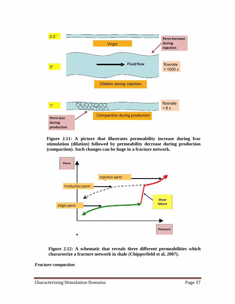
Figure 2.11: A picture that illustrates permeability increase during frac

stimulation (dilation) followed by permeability decrease during production

(compaction). Such changes can be huge in a fracture network.

Figure 2.12: A schematic that reveals three different permeabilities which

characterize a fracture network in shale (Chipperfield et al, 2007).

Fracture compaction


As discussed earlier (Palmer and Moschovidis, 2010) and as illustrated by Figures 2.11

and 2.12, large injection permeabilities are consistent with (a) shear failure and dilatancy,

(b) Walsh model for fracture-dominated flow, and (c) pressure-dependent leakoff

measurements from DFITs. As shown by Figure 2.1, we have found that when a well is

brought on-line, production permeability is only ~1/1000 of injection permeability, which

implies that most of the injection permeability is lost. This serious loss of injection

permeability, due to mechanical compression of natural or induced fractures, is called

fracture compaction.

Figure 2.13: Pressure-dependent leakoff through natural or induced

fractures. In tight sands/shales Cdp = .002-.03 /psi where Cdp is coefficient of

exponential increase with pressure (Ramurthy, private communication,

2010). Since perm increase is of same order as leakoff increase, perm can

increase enormously with injection pressure (these are increases relative to a

base case).

Gel damage

It does not take much of a pressure increase to open up natural or induced fractures in a

fracture network (i.e. they are very compliant), as Figure 2.13 indicates. If the opening is

large enough, frac fluid loss accelerates, and whole gel molecules may leakoff also. In

this case fluid loss into the shale matrix may lead to deposit of gel filtercake on the

surface of the natural or induced fractures. When the frac job is over, the filtercake may

have plugged fractures in the network, perhaps permanently (Britt et al, 2006).

Fines movement and plugging

Fines movement and plugging is a catch-all often used to explain poor wellbore

production. The origins for the fines include:

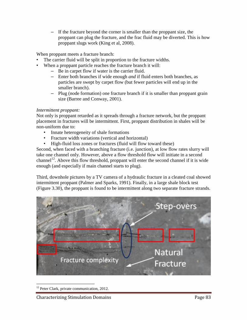
Fracture creation, when chips of rock may spall from a fracture face.

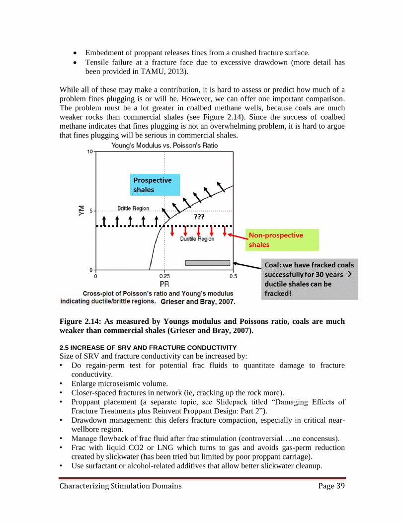
Proppant abrasion of a fracture surface or corner.

Proppant crushing as two fracture surfaces close with pressure drawdown.

Leakoff increase with pressure

1

10

100

1000

10000

100000

1000000

10000000

0 200 400 600 800 1000 1200

Pressure above fissure opening (psi)

Cp

/Co

Cdp = 0.002/psi

Cdp = 0.005/psi

Cdp = 0.01/psi

Cdp = 0.02/psiCdp = 0.03/psi


Embedment of proppant releases fines from a crushed fracture surface.

Tensile failure at a fracture face due to excessive drawdown (more detail has

been provided in TAMU, 2013).

While all of these may make a contribution, it is hard to assess or predict how much of a

problem fines plugging is or will be. However, we can offer one important comparison.

The problem must be a lot greater in coalbed methane wells, because coals are much

weaker rocks than commercial shales (see Figure 2.14). Since the success of coalbed

methane indicates that fines plugging is not an overwhelming problem, it is hard to argue

that fines plugging will be serious in commercial shales.

Figure 2.14: As measured by Youngs modulus and Poissons ratio, coals are much

weaker than commercial shales (Grieser and Bray, 2007).

2.5 INCREASE OF SRV AND FRACTURE CONDUCTIVITY

Size of SRV and fracture conductivity can be increased by:

• Do regain-perm test for potential frac fluids to quantitate damage to fracture

conductivity.

• Enlarge microseismic volume.

• Closer-spaced fractures in network (ie, cracking up the rock more).

• Proppant placement (a separate topic, see Slidepack titled “Damaging Effects of

Fracture Treatments plus Reinvent Proppant Design: Part 2”).

• Drawdown management: this defers fracture compaction, especially in critical near-

wellbore region.

• Manage flowback of frac fluid after frac stimulation (controversial….no concensus).

• Frac with liquid CO2 or LNG which turns to gas and avoids gas-perm reduction

created by slickwater (has been tried but limited by poor proppant carriage).

• Use surfactant or alcohol-related additives that allow better slickwater cleanup.


• Continuously inject nitrogen via injector-producer pairs to maintain high reservoir

pressure to prevent fracture compaction (as is often done in Gulf of Mexico oil

fields). This has not been tried, but should help to retain high injection perms.

First, we point out the disadvantage of foam fracs and gas fracs. Gas (N2 or CO2) and

foamed fluids would seem to be ideal frac fluids for shale: they reduce injected water

volume, and assist in load recovery (energized frac fluids). However they do NOT

stimulate as well as slick-water fracs, as shown by actual well results in Barnett and

Fayetteville. In shales, a good frac fluid needs to invade and enlarge the natural fracture

systems to create a fracture network. Foam has a natural leakoff control through its

increased viscosity and the Jamin effect of hindering flow by bubble deformation. In

contrast, nitrogen and carbon dioxide gas fracs can invade the shale natural fractures, but

they lack the ability to carry any significant proppant while in the gas phase.

Regain-perm test for fluid damage (compatibility)

To lower frac pumping pressure caused by friction, frac water is made slick using

polyacrylamide or linear gel or other chemicals. The “slick” in slickwater can cause

significant perm damage: use as low a concentration as possible. The “slick” is usually

polyacrylamide, which is hard to break. 10 lb guar is much easier to break, but is more

viscous than polyacrylamide slick. Note: all gels and their residue are damaging to some

extent. Therefore a regain-perm test can be used ahead of the frac treatment to test frac

fluid damage to cores. Then we can choose the fluid that causes the least perm damage.

Because shales are so tight, perm damage is largely caused by capillary pressure and

phase trapping by frac fluids in small shale pores. Regain perms are measured using

methane, and they can vary 20 – 100% for common frac fluids (Figure 2.15). The regain

perm also depends on drawdown: a larger drawdown means a larger regain perm (Figure

2.15). Four of the best frac fluids for Montney were two high-quality water-based foams,

a gelled propane, and CO2. This conclusion was not unexpected.

Note however, the cost may not be worth it because each lab test lasts 7 days for

Montney (Figure 2.15), and lasts >7 days for other shales. An alternative decider may be

a field test: frac fluid cost per produced gas generated (although innate variability from

one well to another may distort the result).

Produced water is being used more and more to frac wells. First, disposal of produced

water can be expensive: US $2 to $15 per barrel. Second, water with chlorides >5000

ppm used to be an obstacle, but newer chemicals and treatment has enabled much higher

re-use. This raises another question: How well do friction reducers work in a particular

produced water? One example is from the Woodford shale (Figure 2.16), where the top

four curves are the best friction reducers for this produced water.


Figure 2.15: Best frac fluids are ones with highest regain perms in the Montney

shale (Taylor et al, 2009).


Figure 2.16: Various friction reducers tested in produced water from the

Woodford shale.

Enlarge microseismic (MS) volume

This is easy to implement: by increasing horizontal well length and/or frac volume

pumped (Figure 2.17). There exists a general correlation between gas production and MS

volume (Figure 2.18). However, Barree4 argues that increasing frac volume may have

diminishing returns (due to damage effects), and Barnett field data by Coulter et al (2004)

supports this. But increasing well length always improves performance as demonstrated

by Figure 2.19 in the Fayetteville, which applies in other fields as well.

Figure 2.17: Three ways to increase SRV size and fracture conductivity.

4 Barree, R., private communication, 2011.


Figure 2.18: General trend that shows gas production increasing with MS

volume (Warpinski et al, 2005). Note that the spread in the trend is likely to

reflect different perm enhancements within the stimulated domain.

Figure 2.19: IP gas rate increases with horizontal well length (Engle, 2009).

Reduce fracture spacing in network

Gas rate (IP) versus well length in Fayettville

0

500

1000

1500

2000

2500

3000

3500

4000

0 500 1000 1500 2000 2500 3000 3500 4000

Average horizontal well length (ft)

Avera

ge I

P g

as r

ate

(m

cfd

)


This is the second leg of the triangle in Figure 2.17. The effect of reduced fracture

spacing is illustrated by Figure 2.20

One way to reduce fracture spacing is by hydraulic diversion between perf clusters

(tricky to design). A second way is by simulfracs or zipper fracs or sequential fracs to

raise pore pressure and cause more shear failure between the two parallel wells (i.e. this

will densify MS events). A third way is by diversion using 100-mesh slugs (risky to

implement).

Figure 2.20: Effect of fracture spacing on gas rate and recovery (Warpinski, et al,

2008).

Hydraulic diversion by close-spaced perf clusters: This is a function of the open horizontal interval and treating rate. A typical frac interval

is 300 – 400 ft long, with 1 – 2 ft clusters of perforations at 4 – 6 shots per foot and every

50 – 100 ft. Perf clusters may be selected by using an average spacing or may be

matched to natural fracture locations, depending on how much is known about the

stresses along the wellbore and the behavior of the frac. Fracs appear to initiate more

easily in areas of low stresses and in most areas of natural fractures.

The concept is to induce a frac from every perf cluster at 50-100 ft spacing. This is about

the best we can do assuming pump rates of ~100 bpm. The number of perfs controls the

amount of hydraulic diversion when the full injection rate is reached. Diversion by

perforations involves the number, diameter, and flow efficiency of the perfs. Significant

perf friction first occurs when the ratio of rate to perfs exceeds 0.5 bpm/perf, but

diversion really begins only when rate reaches 1.0 bpm/perf. The most effective

diversion probably occurs at 2.0 – 2.5 bpm/perf.


The pump rate produces the pressure to drive the frac, and multiple frac points (clusters)

require a minimum rate to extend each frac. We normally think of 10-20 bpm per perf

cluster to drive a frac, and this implies that a typical 5 perf clusters in one frac stage

would require at least 50 bpm to open up. Actually the 10 bpm applies to brittle shales,

while the 20 bpm is for ductile shales, so 50 bpm ought to work in brittle shales such as

the Barnett.

Note that extremely low rates (e.g., < 20 bpm) may just open natural fractures and give

very small stimulated reservoir volume, even when large volumes are used. By the same

token, achieving diversion while injection rate is building to design rate (e.g. 100 bpm)

requires diversion by other methods (e.g., ball sealers).

Simultaneous fracturing of two parallel wells.

Simulfracs or zipper fracs or sequential fracs act to raise pore pressure and cause more

shear failure between two (or more) parallel wells. This will create a higher density of

MS events, and should correspond to closer fracture spacing in the network. An example

of this is shown by Figure 2.21.

Figure 2.21: Zipper fracs in Barnett shale in Western Parker County (King et al,

2008).

Diversion by proppant slugs.

Proppant slugs used in the Barnett shale to plug fractures and induce fluid diversion are

typically 100-200 barrels of 100-mesh at 1-2 ppg above ambient concentration (King et


al, 2008). This approach has been used with two purposes: (1) to stop downward fracture

growth into the wet Ellenbarger, (2) to increase MS spread and reduce outward MS

growth away from a well.

The same approach was tried in Canada (Montney shale?) where proppant slugs were

injected to try to stop fractures extending along Shmax, and give a wider microseismic

spread. The technique did not work until the proppant size was increased. 100 mesh gave

no success. 40-70 mesh gave no success. But then 20-40 mesh gave success. This was an

aggressive move, since the risk of screenout increased with proppant size.

Drawdown management

This seems to be important in Haynesville and in Eagle Ford shale plays. If drawdown is

too large, fractures near the wellbore close fast and permeability loss is never recovered

(Abou-Sayed, 2011). In their work in the Haynesville shale, drawdown is kept below a

critical value, especially at early times, using choke management (Figure 2.22). The

critical drawdown is established after careful lab rests, and depends on:

Near-wellbore reference pressure

Minimum horizontal stress

Shale creep

Pressure-dependent permeability

Although reservoir pressure will still hit the critical value at some depletion, the authors

argue that choke management leads to a net benefit over the long term.

Figure 2.22: Drawdown management for EXCO well in Haynesville (Abou-

Sayed et al, 2011)


Figure 2.23: Gas production declines for different wells in Eagle Ford

(Thompson et al, 2012). Steep declines indicate damage from excessive

drawdown.

In Eagle Ford shale, benefits of controlled drawdown include a decrease in first-year

decline from 80% to 50%, more stable production growth, and significant increase in

EUR. The latter would potentially offset diminished present value due to deferred

production5.

Manage flowback of frac fluid

Why does flowback matter? In textbooks a frac treatment is followed immediately by

flowback of frac fluid (Figure 2.24). However, shale wells that recover frac load water

too rapidly may leave water stranded in microfractures where capillary pressure can be

very high. This would reduce permeability to gas and therefore gas flow to the well.

The discussion around flowback from shale wells has not been settled, and more work is

needed. Some opinions expressed circa 2010 include:

• Southwestern Energy: shale gas wells are better if LESS flowback.

• Controlled flowback produced better wells (Dick Leonard and George King in

private communication).

• Devon: after frac stimulation, only inner regions cleanup (regions closer to wells),

while outer regions retain frac water. When two horizontal wells are stimulated

close together (e.g. zipper wells) there is better cleanup of retained water between

the wells which translates to better well productivity.

5 Petrohawk, 2010.


• From production analysis, the effective domain of stimulation is much smaller

than the microseismic domain, due possibly to poor frac fluid cleanup (Barree et

al, 2003).

Figure 2.24: Typical flowback of frac fluid versus time: Barnett shale

Comments by George King (private communication):

• The percent of frac load fluid recovered is about 50% in the Barnett.

• Shut-in time and flowback tests in the field are in a state of flux with a lot of

ideas, but few proven methods.

• Several shales (Marcellus, Haynesville, Eagle Ford, and Utica) are experimenting

with shut-in and controlled flowback.

• Operators report that control of flowback rate to maintain pressure (below critical

drawdown pressure) have been proved in the Haynesville, but are theories

elsewhere.

• Blow-down of shales can result in high IP’s to report to investors, but the fluids

produced do not reflect what is in the formation: initially the light ends and gas

move, but the oil does not.

• One new concept: better control of flowback is needed to preserve reservoir

energy.

Comments by Mike Vincent (private communication):

• There is very little consensus.

• It appears the best practices vary by play, and perhaps by completion type. In the

Bakken for instance, I see superior production and EUR achieved with aggressive

flowback only if the frac is completed with ceramic proppant. On wells treated

with sand or RCS, cautious, conservative flowback appears to be preferable. We

do not know whether the difference is due to flowback of crushed frac sand, or

whether it is simply the challenge of pulling gel debris through the small pore

throats.


• In the Marcellus and Eagle Ford, at least two operators have touted 30-90 day

shut-ins following stimulation. This dissipation period is reported to result in

superior production and less flowback water to handle. However, this practice is

refuted by competing operators.

• Note that strategies to flow back wells after they have been subjected to a 10-day

long frac period using plug and perf techniques, may differ from a well in which

all the stages are completed in just 24 hours.

A “Frac-and-Bake” approach has been used in the Utica shale, where flowback is delayed

for 1-3 months. The resultant oil rate is better by up to five times. One potential

explanation is that imbibed water changes the wettability of shale rock…..making it more

oil-wet.

Frac with liquid CO2 or LPG

These are called “waterless” fracs, to emphasize the issue of enormous quantities of water

that have to be used in slickwater fracs in horizontal wells (several million gallons per

well). They are expensive. Their best application so far has been in shales which are

hyper-sensitive to water.

Liquid CO2 Fracs:

• Carbon dioxide in the liquid or dense phase (carrying sand) has been used in

Devonian shales and outperformed both foam and nitrogen gas fracs (Yost, 1994).

• The production response from the gelled CO2 fracs outperformed nitrogen fracs by

two-fold and water-based foam fracs by about five-fold.

• One shale in the Piceance basin was fracked with liquid CO2 in the 1990s. It was the

best well in the field for a while, but production declined rapidly, possibly because of

too little proppant carried by the very low viscosity fluid.

• Because of its high solubility in both water and oil, and because it lowers oil

viscosity, CO2 may be the most beneficial gas injection to remove both water and oil

blockages.

• Restimulation concept: If the well has left significant amounts of load water in the

fracture network, re-energizing the formation fractures with gas at a pressure below

the frac pressure followed by controlled drawdown may assist with water recovery.

The frac fluid properties in LPG Fracs, plus their advantage or disadvantage, are

displayed in Figures 2.25, 2.26, and 2.27.


Figure 2.25: LPG advantage: surface tension is a lot lower than water (Lestz,

2010).

Figure 2.26: LPG advantage: capillary pressure (220 psi) is a lot lower than

water (2,000 psi) (Lestz, 2010).


Figure 2.27: LPG disadvantage: viscosity is a lot lower than water (Lestz, 2010).

Additives that allow better slick-water cleanup

Small amounts of surfactant or micro-emulsion can sharply increase liquid recovery at

low gas rates (Figure 2.28). The liquid recovery also depends on the gas flow rate: water

expulsion from a fracture increases with increasing gas velocity.

Other comments on moving liquids out of fractures (King, 2010):

• Some specialty additives are beginning to be tested in shale gas applications. The

purpose is to recover water faster and to minimize damage from phase trapping or

water blocks.

• The specialty additives include surfactants, micro-emulsions and specialty

chemicals for reducing interfacial tension.

• Some jobs where micro-emulsion products were used showed better load fluid

recovery and generally higher stabilized gas rates. A few micro-emulsion additives

are made with biodegradable solvent/surfactant/cosolvent and water, and were

originally developed for stimulation and frac fluid recovery in depleted or low

pressure reservoirs.

• In addition, some companies are adding EOR chemicals to the frac to attempt to

both recover more reserves and establish more conductive pathways.

• One operator in the Bakken has used surfactants and micro-emulsions to aid initial

cleanup of fracture face and propped fractures (Pearson et al, 2013).


Figure 2.28: Liquid recovery as a function of gas flow rate through a fracture

packed with proppant: improvement for a surfactant and a micro-emulsion

(Penny et al, 2006).

2.6 CONCLUSIONS OF SECTION 2

General conclusions:

• From DomAnal analysis, when a well is brought on-line, the production perm is

only ~1/1000 of the injection perm, implying most of the injection perm has been

lost.

• The loss of injection perm has potential use as a diagnostic of:

– Frac fluid damage and cleanup

– Proppant design

• Slick-water fracs, which cause less gel damage, can only carry small proppant

loads and proppant will fall out much quicker. However, the advantage of fracture

complexity biases the choice towards slick-water fracs for shale gas (and

sometimes for shale oil).

• We assume a fracture network is created during slickwater frac stimulation, and

we describe damage effects in relation to that network.

• These damage effects have been addressed in terms of their effect on final

stimulated reservoir volume (SRV) size and fracture conductivity within the

network of the SRV:

– What factors reduce SRV size and fracture conductivity

– What factors increase SRV size and fracture conductivity

SRV size and fracture conductivity are reduced by:


• Water imbibition: this raises water saturation and reduces perm to gas. In shales it

is hard to dislodge water because of strong capillary forces in tiny pore throats.

• Fracture compaction: fractures close with drawdown and depletion as pore

pressure is reduced and effective stress increases.

• Polyacrylamide or gel damage in the “slick” of slickwater: polymer or residue can

lodge in network fractures and plug gas flow.

• Fines movement and plugging (fines caused by proppant crushing or grinding of

rock asperities).

SRV size and fracture conductivity can be increased by:

• Do regain-perm test for potential frac fluids to quantitate damage to fracture

conductivity (ahead of the frac treatments).

• Enlarge microseismic volume.

• Closer-spaced fractures in the fracture network (ie, crack up the rock more).

• Proppant placement (this is a separate topic, see chapter 3 below).

• Drawdown management: this defers fracture compaction, especially in the critical

near-wellbore region.

• Manage flowback of frac fluid after frac stimulation (controversial….no

concensus).

• Frac with liquid CO2 or LNG which turns to gas and avoids gas-perm reduction

created by slickwater (has been tried but limited by poor proppant carriage).

• Use surfactant or alcohol-related additives that allow better slickwater cleanup.

• Continuously inject nitrogen via injector-producer pairs to maintain high reservoir

pressure to prevent fracture compaction (as used in oil production in GOM fields).

Not been tried, but should help to retain high injection perms.

3. PROPPANT TRANSPORT IN A FRACTURE NETWORK 3.1 INTRODUCTION

The goal in this chapter is to analyze proppant transport in a fracture network, to re-

invent proppant design applicable to gas shales. A small amount of proppant (i.e. a

partially propped fracture) can increase the fracture conductivity enormously, as we have

discussed. How to get proppant into a network of fractures, with good coverage, becomes

a critical aspect. The deliverable is a simplified but practical theoretical analysis and

report of proppant transport in a fracture network, including access to fractures, and

penetration into fractures. The emphasis remains slickwater fracs or hybrid fracs that

initially use slickwater to create a fracture network.

3.2 INFORMATION ON PROPPANT FROM WELLS IN SHALE PLAYS

George King perspective6

Much of the information below comes from King, 2010, and King et al, 2008. Further

details are available in these publications.

• As deeper shales are investigated, sand may not give adequate conductivity at the

higher stresses and may give way to higher strength proppants and more high-tech

6 George King, 2012, private communication.


fracturing designs. There is no set formula for a shale frac, even in a specific area.

Every well is different.

• One-hundred mesh sand has been used in fracturing to stop downward fracture

growth, particularly when the size of the pad (no sand) is curtailed and the rate is

reduced. It has also been used in mixtures with other sands to bridge-off larger

fractures (King, 2008). The mechanism behind reducing downward frac growth may

have many explanations, but is generally thought to form a wedge with 100 mesh

sand slugs in the fracture preventing excessive downward or, sometimes, outward

growth.

• The loading or ramping of sand in a shale gas frac job is very shale play dependent.

Frac width is the primary control on bridging potential in the near wellbore part of the

fracture. Width depends on rate, fluid viscosity, formation brittleness, local stresses

and if the pay zone is bounded by effective frac barriers. Typically, an initial loading

of 0.2 to 0.25 lb/gal is a starting point with common increases of 0.25 lb/gal possible

after pressure stabilizes. Upper limit on the proppant concentration in the carrier fluid

depends on the proppant size (both carrying capacity and frac width limited), and is

often in the 2.5 lb/gal range for 100 mesh sand and 2 lb/gal for 40/70 mesh. Actual

ranges will vary with application.

• Application of slugs of proppant for control of leakoff is an older technique brought

to both oil-rich shale and gas shale fracturing (Wiley et al, 2004; King, 2008). A

typical slug is 0.5 to 1.5 lb/gal over the programmed sand loading level and carries on

for only 100 to 150 bbls. The effect of the slugs may not be seen immediately but are

often noticed a few minutes after the slugs hit the perforations. Some appliers have

used proppant slugs and ball sealers in unison, but this appears to be rare (Wiley et al,

2004).

• Larger proppants, if used, are usually placed at the end of the frac stage; however, this

arrangement does not assure that the larger sands will be closer to the wellbore to

increase conductivity. Because of the dune formation of sand deposition by fluids that

sweep the proppant along rather than carry it, the last particles carried into the

fracture may end hundreds of feet away from the wellbore (Leonard et al, 2007).

Sand transport prediction and assessment has been attempted by a number of authors

and the general finding is that Stoke’s Law is inadequate to describe proppant

transport in shale fracturing.

• Alternative proppants (non-sand) have included small mesh bauxite for erosion and

bottom barrier formation, medium-strength man-made proppants, and light-weight

proppants.

• A very wide range of overflush volumes using base frac fluid (no sand) have been

trialed. Volumes as low as 20 bbls over the casing volume to the lowest perfs have

demonstrated little or no sand blocking in the wellbore on post-frac pump-down

operations, while very large volumes of post flush have not shown any advantage

over the smaller volumes. Regardless of the volume used, the rate of displacement

should be the same as during the frac treatment.

• Pressure changes during the job are used by some appliers as an indicator of frac

quality, but this is not agreed upon over the whole frac spectrum. Those that use the

indicator argue that a net pressure rise of about 700 to 1000 psi net (corrected for

fluid slurry column density and friction) is an indicator of a frac that is building


complexity in zone. A number of tests have arrived at general conclusions that

increasing pressure and complexity may be related (Warpinski et al, 2008).

Chipperfield et al, 2007), as pointed out in other places of this report, provides

interesting observations and modeling about sub frac-pressure complexity generation

that may have an impact in shale frac design. In frac experience in the Barnett shale, a

modest net pressure rise of 1 to 5 psi per minute has been correlated with an increase

in complex fracture development (a width over length complexity development ratio),

fracs staying in zone without a lower frac barrier, and decent production increases

compared to offset wells of high tech operators (King et al, 2008). No doubt there are

other factors involved in the well performance. A more rapid net pressure rise of 8 to

15 psi per minute has been linked to what appear to be potential screenouts and some

cases of breaking out of zone following the sharp pressure rise (King et al, 2008).

• The amount of sand used in most water fracs in gas shales has been steadily

increasing throughout the industry. Problems that remain unresolved include success

of proppant placement in the smaller fissures and effectiveness of proppant over the

life of the well. Several studies on production response have indicated that the

primary fractures are probably propped by the slickwater fracs, but the secondary

fracs are probably not being propped.

More proppant is better

In the Barnett shale, more proppant is better, as indicated by Figure 3.1.

Figure 3.1: Gas rate versus proppant amount from different wells (Smith,

2007). The data set with black squares is from Coulter et al (2004).


Figure 3.2: Gas rate versus proppant amount per unit length, from two different

shale basins (Hennings, 2010).

However, in at least one shale basin, the trend is for a lower gas rate with higher proppant

amount, as shown by Figure 3.2 (although the correlation is weak).

In the Marcellus shale, long horizontal wells were cased and perforated, 6-8 frac stages

(3-4 perf clusters per stage), and fracs were pumped at 50-100 bpm. “Lite” fracs have

only ~1/5 sand amount (and all 100-mesh), but the same water volume as “Offset” fracs

which use 100-mesh followed by 30-50 proppant. Microseismic maps reveal similar frac

complexity. Figure 3.3 demonstrates that gas production from Lite frac wells is much

lower than Offset frac wells, implying reduced fracture conductivity in Lite frac wells

due to less total sand and/or smaller sand size. Again, more proppant (and possibly larger

proppant) boosts gas production.


Figure 3.3: Gas rate versus production time for two different well completions. The

lower points correspond to “Lite-Fracs” and have less proppant and smaller

proppant (Curry et al, 2010).

In the Fayetteville shale, a statistical study has been made of many wells (Xiao et al,

2012). EUR was calculated in ~2,000 wells, and correlations sought with depth,

geological area, proppant volumes, etc. In 2009, the top-quartile of well performers used

a mean of 3.9 mm lb proppant cf. a mean of 2.7 mm lb for the bottom quartile (Figure

3.4). More proppant is better, but there is a large overlap due to production variability.

In the Bakken, Baker-Hughes have studied variables affecting production in 3,000 wells

(Lafollette et al, 2013). In order of importance, the variables affecting well production

were found to be:

• Well location

• Volume of fracturing fluid

• Use of coarse proppant

• Proppant concentration

From other discussions, the last two bullets may suggest that in the Bakken near-wellbore

conductivity is more important than a far-field fracture network.

In the Bakken, Liberty Resources have reported results from horizontal wells with ~9500

ft length, and up to 30 frac stages, using perf clusters in cemented casing (Pearson et al,


2013). Only slickwater frac fluid was pumped at 70-80 bpm to create fracture

complexity. Premium ceramic proppant was used to maintain fracture conductivity at

9000 psi total stress and 250F, because crush tests revealed orders-of-magnitude

difference in fracture conductivity between ceramic and sand. The authors expect a

monolayer distribution of proppant at < 1 lb/ft^2. Wells completed in this way produced

30-50% more oil production than offset wells which used hybrid fracs (i.e. slickwater

ahead of gel).

Figure 3.4: Tier 1 versus Tier 4 quartile well performance, and difference attributed

to total proppant amount (Xiao et al, 2012).

In the Haynesville shale, Exco have reported results from horizontal wells (~4000 ft)

which have 10-18 stages plus 4-9 perf clusters/stage (Abou-Sayed, 2011). Vertical depth

is about 12,000 ft, Po = 0.91 psi/ft, Pclos = 0.95 psi/ft, Ko = 4 µd. Natural fractures seen

in image logs motivated the operator to use 100-mesh proppant to plug these secondary

fractures, in order to create longer transverse fractures. Lab tests revealed shale creep

causing fractures to close (when conductivity falls by ~100 times) and proppant to embed

in the softer formation. To offset this the operators used premium ceramic proppant to

maintain fracture conductivity at 11,000 psi total stress and 300F (from lab tests). This

conductivity is better than sand by 2-10x in the lab. Drawdown management was also

implemented (via choke control) and this reduced rapid production decline at early times.

In the Fayetteville shale, Southwestern Energy analyzed gas production from 26 pairs of

wells stimulated with slickwater fracs (Rassenfoss, 2012). In general 100-mesh sand was

used ahead of 30-70 mesh proppant. In all these wells, everything was kept the same

except the proportion of 100-mesh and 30-70 proppant. Results of the analysis were:

• 5 wells with all 100-mesh produced roughly the same as wells with all 30-70

proppant. This is the same result as in the Cadomin (a tight sand in Canada), where


one well with all 100-mesh produced just as well as one with 100-mesh followed by

40-70 proppant.

• Compared with 100% of 30-70 proppant, 5 wells with 50:50 proportion were down

15%, but 16 wells with 50:50 proportion were up 27%.

• A 50:50 proportion of 100-mesh followed by 30-70 proppant is better than 100% of

100-mesh or 100% of 30-70.

• Possible explanations: (1) a spectrum of crack opening widths exists in the fracture

network, and using both 100-mesh and 30-70 proppants allows propping a larger

number of fractures, (2) 100-mesh proppant is carried out farther and props more

smaller fractures, while 30-70 props better fractures closer to wellbore.

Although not a shale, a well drilled into the Pictured Cliffs sand in the San Juan basin, by

Energen Resources, provides insights that are relevant to proppant use in shale wells

(Ramurthy et al, 2013). Details of the frac fluid and proppant are:

• There was limited space on the drilling pad.

• N2-foam fracs were pumped at 25 bpm.

• The operator used only 31,000 lb of ultra-lightweight proppant compared with

296,000 lb sand in a previous well (i.e. they switched from 15 trucks of regular sand

to 1 truck of ultra-lightweight proppant).

• The ultra-lightweight is called MonoProp and is made of thermoplastic alloy.

• The result was better gas production in this well.

• The author’s interpretation was that the ultra-lightweight proppant gave larger

conductivity (due to partial monolayer coverage) and probably deeper penetration in

the fracture compared with regular sand.

Summary of above section:

• More proppant is better. Probably because it helps retain the created conductivity of

fractures in the network (the injection permeability can be hundreds of md).

• Premium ceramic proppant is preferred by two operators (Bakken and Haynesville) to

maintain fracture conductivity in deep, hot shales with total stress 9,000-11,000 psi

and 250-300F (based on conductivity in lab tests).

• In the Fayetteville, a 50:50 proportion of 100-mesh followed by 30-70 proppant is

better than 100% of 100-mesh or 100% of 30-70. There are two possible

explanations.

• Ultra-lightweight proppant gave larger conductivity (partial monolayer) and probably

deeper penetration in a fracture compared with regular sand (a Pictured Cliffs well in

the San Juan basin).

• Coarser proppant of higher concentration (tail-in?) gives better results in the Bakken.

Perhaps this is because near-wellbore conductivity is more important than far-field

conductivity in this shale.

3.3 CONDUCTIVITY OF FRACTURES WITH PROPPANT

A small amount of proppant in a fracture can boost the conductivity of a fracture many

times. We must first distinguish between the types of proppant packing in a fracture.

Textbooks talk of proppant packs, where a few or several layers of proppant exist. If only

one layer of proppant exists, this is called a monolayer. If proppant grains are sparser

than a monolayer, this is called a partial monlayer (Figure 3.5).


Figure 3.5: Partial versus full monolayer (Brannon et al, 2004).

Figure 3.6: Possible geometry in field (left) and partial monolayer in core (right)

(Brannon et al, 2004).

Partial monolayers of proppant

In shale formations, which are very heterogeneous at all scales, proppant is likely to be

intermittent (see picture in Figure 3.6, left side). At core-scale, a partial monolayer looks

like Figure 3.6 (right side). The questions are:

• Can we create in the field a uniform partial monolayer like the photo at right of

Figure 3.6?

• Will we create pylons or clumps of proppant at pinch points such as in Figure 3.6

at left?

• Can we sustain open channels if proppant not evenly distributed (Figure 3.6, left)?

The advantage of a partial monolayer is the boost in fracture conductivity, as represented

by the bumps in Figure 3.7. However these bumps become less of a boost as the closure

stress increases (4000 psi is the usual standard).


Figure 3.7: Partial monolayer conductivities (Brannon et al, 2004). Partial

monolayer conductivities are the bumps at the left ( < 0.06 lb/ft^2).

Figure 3.8: Partial monolayer of a new ultra-light-weight proppant (ULWP) called

FracBlack (Sundrilling.com). Can use up to 220F.

• Another example of a partial monolayer is shown in Figure 3.8. In this case the

proppant density is very close to water (1.08 SG), and so this ULWP is expected

to be carried much deeper into the fracture(s). ULWPs are connected to partial

monolayers in field experience, probably because the proppant is expensive and


the amount used is much less. One example is provided above in the section

More proppant is better (a well drilled into the Pictured Cliffs sand in the San

Juan basin). Several recent papers have reported good field performance using

ULWP, and there is increasing demand for engineered ULWPs. However, “My

experience has been fairly poor using ULWP as a stand-alone proppant. I’ve only

seen success using ULWP in conjunction with standard rigid proppants”.7

Partially propped fractures: Fredd results

The huge advantage of partially propped fractures is summarized by lab tests in Figure

3.9. With reference to a displaced fracture with no proppant, the conductivity upside of

0.1 lb/ft^2 sand is 1.5-2 orders of magnitude. The conductivity upside of 0.1 lb/ft^2

bauxite is 2-3 orders of magnitude.

Figure 3.9: Fracture conductivity versus closure pressure for different proppants

and fracture geometries (Fredd et al, 2001). A displaced fracture has some shear slip

along the fracture length, which increases its conductivity (this phenomenon is

called dilatancy).

Fracture conductivity boost by proppant: Dan Hill et al.

Comprehensive lab tests with Barnett Shale have recently been published (Zhang et al,

2013). They measured gas flow through a fine crack in core under reservoir conditions.

Adding 100-mesh proppant, in only a small amount, increased the gas flow by 100 times.

Increasing closure stress reduced the gas flow. To summarize their tests and results:

7 Mike Vincent, private communication, 2012.


• They used mostly 100-mesh or 40-70, but a few tests with 30-50.

• Proppant concentrations ranged 0.03 - 0.15 lb/ft^2 corresponding to 0.25 - 1.25 ppg.

• For 100-mesh sand, full monolayer requires >0.05 lb/ft^2.

• Unpropped induced fractures and poorly-cemented natural fractures are conductive in

shales, but the conductivity is very low ~0.5 md-ft.

• Propped fracture conductivity is more than 10 times this at 4,000 psi closure stress,

and increases from 100-mesh to 40-70 mesh proppant.

• Fracture conductivity also increases with proppant concentration.

• Partial monolayers are uneven: proppant accumulates in “valleys” and may act as

pylons to prevent fracture closure (Figure 3.10).

• Proppant conductivity in Barnett core can fall by 20% due to creep over 20 hours

before it flattens (it should fall more in softer shales like Haynesville).

• It was hard to achieve a partial or full monolayer in a horizontal fracture. The rough

surface causes grains to roll from peaks into valleys multiple layers of grains in

valleys with a possible monolayer at peaks (Figure 3.10).

Figure 3.10: Uneven proppant distribution in horizontal fracture: partial monolayer

concentration of 0.03 lb/ft^2 (Zhang et al, 2013).

• At 4,000 psi closure, 0.06 lb/ft^2 of 100 mesh has higher conductivity by almost 2

orders cf. unpropped fracture (Figure 3.11).

• At 4,000 psi closure, 0.06 lb/ft^2 of 40-70 mesh has higher conductivity by over 2

times cf. 0.06 lb/ft^2 of 100-mesh (Figure 3.11).

• At higher stress, surface roughness is deformed and reduced, making the discrepancy

with proppant greater (Figure 3.11).

• Conclusion: need to use proppant in shale fracs, and larger proppant is better IF it can

fit into fractures.

• For either 100-mesh or 40-70, conductivities are ~7 x higher at 0.15 lb/ft^2 compared

with 0.06 lb/ft^2 (Figure 3.11) conductivity increases with proppant size and even

more strongly with concentration (100-mesh and 40-70).


Figure 3.11: Conductivities of displaced fracture: unpropped and propped by 100-

mesh or 40-70 mesh sand at 0.06 lb/ft^2 or 0.15 lb/ft^2 (Zhang et al, 2013).

An uneven distribution of proppant over a fracture surface leads to greater fracture

conductivity (Figures 3.12 and 3.13). Shale formations are very heterogeneous, at all

scales, and it follows that fractures (in a fracture network) will be heterogeneous also,

leading to an uneven distribution of proppant. One explanation is that multiple layers of

proppant in wider “valleys” or collected at pinch-points act as pylons to keep the fracture

open. Given this, the trick is to get proppant into as many fractures in the network as

possible.

Finally, Figure 3.14 reveals that the classical partial monolayer boost for fracture

conductivity is only seen for closure stress ≤ 2,000 psi, which will be rare for most

commercial shale plays. The main thrust of Figure 3.14 is that the conductivity of 100-

mesh sand increases with proppant concentration, even if the proppant is distributed

unevenly (i.e. pylons). Therefore we should try to increase the concentration (in ppg) of

injected 100-mesh sand during a frac treatment. The result also suggests that 200-mesh

sand, which should be carried easier and further into a fracture network, may give rise to

higher concentrations than 100-mesh sand (and the benefits of Figure 3.14).


Figure 3.12: Proppant distribution using 100-mesh sand at 0.03 lb/ft^2: (a)

proppant migration in sample 20, (b) evenly distributed proppant in sample 18

(Zhang et al, 2013).

Figure 3.13: Conductivities of aligned fractures propped by 100-mesh sand at

0.03 lb/ft^2 (Zhang et al, 2013). Samples 18 and 20 are as shown in Figure

3.12. Uneven distribution of proppant is better.


Figure 3.14: Conductivities of displaced fractures propped by 100-mesh sand: (a)

versus closure stress, (b) versus proppant concentration (Zhang et al, 2013).

Figure 3.15: Conductivity uplifts and their effect on gas production (Cipolla, 2009).

Figure 3.15 is an example of production improvement as a function of fracture network

conductivity. An increase of conductivity from 2 md-ft to 5 md-ft would give a 50%

production increase (e.g. from 2 MMcfd to 3 MMcfd). This is huge. An increase of

conductivity from 2 md-ft to 10 md-ft would give a 100% production increase (e.g. from

2 MMcfd to 4 MMcfd).

Fracture conductivity versus proppant geometry

Fredd’s conductivity upside was due to partial propping (ie, partial monolayer –Figure

3.5). Now the conductivity depends on the width of the open (partially propped) fracture.

If this conductivity were 100 md-ft for a fracture held open by 40-70 sand, it would be

only 55 md-ft for 100-mesh sand (Figure 3.16). This is based on mean grain diameters,


and ignores embedment. However if 100-mesh grains clump into pylons at corners or

constrictions or in valleys (or other heterogeneities), that could possibly raise fracture

conductivity by several times (Figure 3.17).

Figure 3.16: Proppant sizes (M. Vincent, 2012, private communication).

At the other extreme from a partial monolayer, we have fracture conductivity when the

fracture is filled with a proppant pack. Lab tests done at TerraTek lab used 100-mesh or

40-70 mesh or a mix of the two (left panel of Figure 3.18). At 4000 psi stress, 40-70

fracture conductivity = 300 md-ft cf. 100-mesh = 60 md-ft. Thus 40-70 is better by 5

times than 100-mesh, but this is a proppant pack with embedment (not a partial

monolayer). The ratio should be less than 5 for a partial monolayer (see Figure 3.16),

although embedment was not included. Note that the panel on the right of Figure 3.18 is

misleading, because it is normalized. The left panel shows that 40-70 proppant gives 5

times greater conductivity than 100-mesh proppant. The issue is to what extent 40-70

proppant is limited in access to finer fractures in the network (but where 100-mesh can

gain access). What our previous discussion has shown is that some proppant, even

smaller proppant, is better than no proppant.


Figure 3.17: Proppant distributions (Cipolla et al, 2008).

Figure 3.18: Fracture conductivities with a proppant pack versus closure stress:

different proppant sizes (TAMU, 2013).


Summary of above section (on conductivity of fractures with proppant)

• Partially-propped fractures provide a huge advantage. Conductivity upside of 0.1

lb/ft^2 sand is 1.5-2 orders of magnitude. Conductivity upside of 0.1 lb/ft^2 bauxite is

2-3 orders of magnitude.

• It is hard to achieve a partial or full monolayer because in a horizontal fracture the

rough surface causes grains to roll from peaks into valleys. This gives multiple layers

of grains in valleys plus possible monolayers at peaks. Partial monolayer

conductivities are uneven: proppant accumulates in “valleys” and may act as pylons

to prevent fracture closure.

• At higher stress, surface roughness is deformed and reduced, making greater the

discrepancy between unpropped and proppant fractures. We need to use proppant in

shale fracs, and larger proppant is better IF it can fit into the fractures.

• Unpropped fracture conductivity falls quickly with stress meaning the conductivity of

100-mesh sand dominates as closure stress increases.

• The conductivity of 100-mesh sand increases with concentration (ppg), which

suggests to try to increase the ppg of 100-mesh sand during a frac treatment.

• Pylons of 200-mesh sand may act in the same way as 100-mesh, but 200-mesh has the

benefit that it can be carried further into a fracture network.

• For a partially propped fracture, the conductivity depends on the width of the fracture,

which is related to proppant grain width. If this is 100 md-ft for fracture held open by

40-70 sand, it would be only ~55 md-ft for 100-mesh sand, based on mean diameters

(but this ignores embedment).

• But if 100-mesh clumps into pylons at corners or constrictions (or other

heterogeneities), that could raise fracture conductivity by several times.

• For a proppant pack, at 4000 psi stress, 40-70 fracture conductivity = 300 md-ft cf.

100-mesh = 60 md-ft. Thus 40-70 is better by 5 times, but this is a proppant pack with

embedment (not a partial monolayer). The ratio may be less than 5 for a partial

monolayer, depending on embedment.

• A 40-70 proppant pack gives 5 times greater conductivity than 100-mesh proppant

pack. The issue is to what extent 40-70 proppant is limited in access to finer fractures

in the network (but where 100-mesh can gain access). What our previous discussion

has shown is that some proppant, even smaller proppant, is better than no proppant.

3.4 PROPPANT SPREADING AWAY FROM HORIZONTAL WELL

The problem is illustrated by Figure 3.19, where the injected frac fluid gets out to the

edge of the microseismc cloud, but the issue is how far out does proppant get? The

proppant spread away from a multi-stage fracture stimulation is determined by several

factors: (1) proppant size, density, and concentration, (2) fracture spacing and width, (3)

fracture pump rate. In the first part of this section, we review the literature. Even though

there is not enough information from lab and field to model proppant spreading, we can

utilize what is available to build a conceptual model which provides trends that should be

of use to an operator in choosing proppant.


Figure 3.19: Schematic of frac fluid spreading from a horizontal well (red arrows).

Conductivities of unpropped fractures

The first point to make is that unpropped fractures, even those which have undergone

dilatancy by shear slip, retain only small conductivities once closure stress is applied. For

an average closure stress of 4,000 psi, which is a common standard for comparison,

Figure 3.9 shows that the conductivity is 1-3 md-ft for a tight sand (displaced fracture).

This is an order of magnitude larger than ~0.1 md-ft for unpropped fractures in tight sand

tests (Britt and Smith, 2009). The latter figure is supported by TAMU (2013) who find

0.2 md-ft for unpropped fractures from shale lab tests. These authors state clearly that

unpropped fractures do not contribute significantly to shale gas production. For example,

they quote that 2,000 psi closure pressure will destroy conductivity in unpropped

fractures in Barnett, Haynesville, and Marcellus rock. This implies that the onus is on a

widespread distribution of proppant to maximize gas production from a network of

fractures.

How widespread is proppant in a slickwater stimulation?

A small amount of proppant in a fracture can boost the conductivity of a fracture many

times. The goal therefore is widespread distribution of proppant throughout the created

fracture network (Figure 3.19). A critical factor is whether proppant particles can fit into

the network fractures with smaller-widths. Just as critical is how far proppant can spread

across the fracture network, and this depends on the factors listed above (and in Figure

3.19). The DomAnal software calculation of fracture network spacing and aperture width

can assist in assessing both of these critical factors.

What determines where proppant goes?

• It tends to fall out rapidly if using slickwater as frac fluid and normal-density

proppant (i.e. sand).

• Even though we calculate an average fracture width and spacing from matching the

microseismic spread in DomAnal, these attributes must be part of a spectrum in a


realistic fracture network (Figure 3.20). See also Gayle et al (2007) for a fractal

spectrum of fracture widths measured in core.

• The role of 100-mesh ahead of 40-70 mesh proppant is (by reference to Figure 3.20):

– 100-mesh can access smaller-width fractures (which 40-70 proppant cannot)

at early time or at larger distance from the well

– 100-mesh can retain more of the injection permeability in these fractures by

(1) partial propping, and/or (2) pylon propping

• The role of 40-70 proppant after 100-mesh is:

– 40-70 mesh can access and prop larger-width fractures more effectively than

100-mesh can (ie, ensuring greater conductivity)

Figure 3.20: Dendritic or fractal patterns in a fracture network (BJ advertisement),

illustrating proppant access issue.

Complex fractures in large block test8:

A water frac in a large block test (~1m across) resulted in complex fractures that were

very widespread (including horizontal fractures). Fracture widths were 0.01 – 0.1 mm =

10-100 μ (previous slide). 100 μ is lower limit for 100 mesh sand which means that 200-

mesh sand would be needed to enter these fractures.

8 Private communication, TerraTek, 2012


How much of a fracture network is propped?

Based on microseismic data, only 5-15% of fractures in a network are propped according

to Cipolla et al, 2008). This might explain why an SRV has a volume that is only ~10%

of the microseismic volume (according to rate-transient analysis of SWN wells by

DomAnal in a later chapter).

Water fracs in hard-rock mineback (Jeffrey et al, 2009)

Below is a brief summary of information relevant to our report:

• The tests were done in a goldmine in Australia, where Sv is minimum stress (2175 psi

vs >2900 psi for horizontal stresses). Stress difference is >725 psi.

• Most induced fractures are horizontal, due to stress anisotropy.

• It is more difficult to inject proppant (100-mesh and 30-60 size) with water fracs,

compared with X-L gel fracs.

• Only 10-15% are fracture branches and sub-parallel propped sections (Figure 3.21).

This is likely because the stress difference is so high.

• One horizontal fracture has a small branch or bifurcation, and both branches contain

proppant (Figure 3.22).

• Most fractures are horizontal segments with offsets as fractures grow up and along

dipping veins and shear zones.

• 100-mesh and 40-70 mesh proppant are found along these offset (and non-offset)

segments. But higher-angle offsets are less propped or are unpropped.

• Modeling showed width of offset falls as angle of offset increases. This implies

higher pressure in such flow constrictions, and larger widths in associated horizontal

fracture segments.

• In shale fields where the maximum stress is vertical and horizontal stresses are not

much different, we would expect more than 10-15% fracture branches and sub-

parallel propped sections. We would also expect widths of offsets to be not much

smaller than main fracture segments. Therefore in shale fields we would expect a

wider distribution of proppant, although the penetration of proppant may be restricted

by having to turn more corners (this we call tortuosity).


Figure 3.21: A portion of Fracture 8 with three sub-parallel fractures

containing proppant (white arrows). Overall, branches and sub-parallel

fractures were only 10-15% of all mapped fractures in this gel-fracture

stimulation (Jeffrey et al, 2009).

Figure 3.22: A portion of Fracture 9 with a small branch or bifurcation. Both

strands appear to contain proppant, shown by red (Jeffrey et al, 2009).


Figure 3.23: Extrapolation of Jeffrey et al (2009) mine-back to Barnett Shale.

Update on mineback study9:

• The fracture network consists mostly of localized flow channels with offsets

(doglegs) plus just a few parallel fracture branches (each has dye but usually only one

has proppant).

• Minebacks of coalbed methane fracs usually reveal only one main fracture strand

contains proppant, although many other strands do contain dye.

• Microseismic events are shear failures which occur away from the flow channels and

are caused by pressure-dependent leakoff.

• These shear fractures may not open up enough to take all proppant sizes (but may

take 100-mesh).

In extrapolating the gold mineback to the Barnett shale, both fracture branching and

fracture offsets should be much more common, because two horizontal stresses are less

than the vertical, and are about equal. This implies a more complex fracture network in

the Barnett shale, as exhibited by widespread microseismic (MS) events.

9 Jeffrey, R., private communication, 2011.


Figure 3.24: Conceptual model of T-shaped fracture in coal (map view). The vertical

fracture has offets (doglegs) and multi-strands (Palmer, 1992).

Water fracs in coal

This subject was studied extensively in the 1980s and 1990s. Figure 3.24 shows an old

conceptual model of a complex fracture in coal, based on a variety of data, including high

frac pressure and mineback views of underground fractures. The complexity is expected

because coal is a naturally fractured formation (the fractures are cleats). However, the

picture applies more to foam fracs, rather than water fracs where mineback data is scarce.

Water fracs if confined to a coal seam are expected to be more complex than Figure 3.24

reveals, and unpublished MS data support this.

We conclude that for foam fracs, proppant spreading is limited, as illustrated by Figure

3.24, although the dye in the frac fluid may be more widespread. However for water

fracs, confined to coal, the proppant may be more widespread. These conclusions apply

to coalbed methane minebacks in the Warrior basin (where horizontal stress is roughly

isotropic). Finally, a downhole TV visualization of fractures in coal and bounding zones

revealed that proppant can be spatially intermittent in coal (Palmer, 1992). These

concluding remarks support that proppant spreading is more limited than frac fluid

spreading, and the cause is likely to be tortuosity of proppant flow through a network of

fractures.

Modeling by Schlumberger

The UFM model by Weng et al (2011) appears to require as input a stochastic set of

natural fractures, which the hydraulic fracture interacts with to create an induced fracture

network. The model implements 1D fluid flow and proppant transport in the fracture

network, using assumptions similar to those for pseudo-3D fracture models. Proppant

transport for slickwater frac fluids consists of a proppant bank at the bottom of the

fracture, a slurry layer in the middle, and clean fluid at the top, for each element of the

fracture network. Modeling results (Figure 3.25) reveal that only a small fraction (2-5%)

of the induced fracture network is occupied by proppant. The reasons are rapid proppant

settling, and proppant bridging in the side fractures which have small aperture width.

Cipolla et al (2010) have argued in this case that only the propped area contributes to


production. This supports our position, based on transient rate analysis (see later), that the

final SRV volume is only ~10% of the initial MS cloud volume.

Figure 3.25: Fracture width contours (left panel) and proppant concentration

contours (right panel): after Weng et al (2011).

Summary of this section (on proppant spreading away from horizontal well)

• Unpropped fractures do not contribute significantly to shale gas production. This

implies that the onus is on a widespread distribution of proppant to maximize gas

production from a network of fractures.

• Based on microseismic data, one estimate is that only 5-15% of fractures in a network

are propped. This is supported by a detailed model of proppant transport which gives

only 5%. These results can explain why an SRV has a volume that is only ~10% of

the microseismic volume (according to gas rate matching of actual wells by

DomAnal). From the detailed model, proppant occupies only a small portion of the

fracture network surface due to (1) rapid settling in slickwater, and (2) bridging in

side fractures of very small width.

• For a spectrum of fracture aperture widths, the role of 100-mesh ahead of 40-70

proppant is:

o It can access smaller-width fractures (which 40-70 proppant cannot) at early

time or at larger distance from the well

o It can retain substantial conductivity in these fractures by (1) partial propping,

and/or (2) pylon propping.

o The role of 40-70 proppant after 100-mesh is to access and prop larger-width

fractures more effectively than 100-mesh can (i.e., giving larger conductivity)

• 100-mesh proppant can access more fractures than 40-70, but loses only a factor of

~2 in conductivity (assuming partial propping and no embedment). If 100-mesh (or

40-70) clumps into pylons it could possibly raise fracture conductivity by several

times.


• Gel fracs in hard-rock mineback: Only 10-15% are fracture branches and sub-parallel

propped sections, partly because vertical is the minimum stress and stress anisotropy

is high. For slickwater fracs in shale formations where vertical is maximum stress and

horizontal stresses are not much different, we expect much more than 10-15%

fracture branches and sub-parallel propped sections. We also expect widths of offsets

to be not much smaller than main fracture segments. Therefore we can expect

proppant to be more widely distributed than in the hard-rock mineback.

• In a large block test, water fracture widths were 0.01 – 0.1 mm = 10-100 μ. Since 100

μ is lower limit for 100 mesh sand we would need 200 mesh sand to enter these

fractures.

• Proppant spreading appears limited, even when frac fluid dye is not limited, in most

coalbed methane minebacks in the Warrior basin (where horizontal stress is roughly

isotropic).

• This lies in agreement with:

o Hard-rock mineback interpretations

o Schlumberger modeling

o Peter Clark lab tests and interpretations (see later)

o High frac pressure in coalbed methane and shale wells: if vertical fracture has

offsets and multi-strands, this can account for abnormally high but steady frac

pressure. But if fracture complexity is increasing, frac pressure should rise in

concert.

• We conclude, for several reasons, that proppant spread away from a horizontal well

will be smaller than slickwater spread and microseismic spread. The corollary is that

200-mesh will spread more than 100- mesh which will spread more than a 40-70

mesh tail-in (Figure 3.26).


Figure 3.26: Picture of proppant spreading versus slickwater spreading

(modified from Fisher et al, 2002).

3.5 THEORETICAL ASPECTS OF PROPPANT TRANSPORT IN A NETWORK

Proppant segregation: settling and convection

As summarized by Figure 3.27, proppant movement is controlled by (1) individual

particle settling, and (2) convective movement of particle slurry. If proppant grains have

a density less than water, they may actually rise slowly as they are carried by the frac

fluid. This compares with normal sand densities which can fall out in 6 cp frac fluid at 2-

3 ft/min, which is quite rapid.

The lower panel of Figure 3.27 indicates that an artificial proppant barrier (bank of

particles) can be designed to inhibit fracture height growth. This is due to a high

resistance of particle movement plus a restricted transmission of fluid pressure to the

fracture tip.

Another mechanism is carpet flow, also called river-bed flow or saltation. Here sand can

be carried a long way beyond that due to individual particle settling when grains

hopscotch along at the top of a proppant bed. For example, sand proppant has been found

>1,000 ft from a vertical wellbore in a coalbed methane well after a slickwater frac10

.

10

Console, private communication, 1995.


Figure 3.27: Two different modes of proppant transport depending on grain density

and fluid viscosity: 6 cp in top panel; >6 cp in bottom panel (Barree and

Mukherjee, 1995)

Proppant bridging or plugging in side fractures

Plugging occurs when a proppant grain is larger than a side fracture, while bridging refers

to grains that can access a fracture, but coagulate at some point just inside the fracture.

Plugging and bridging act the same: they divert frac fluid to other existing branches or

force it to create new branches. This can increase fracture network complexity and raise

pumping pressure. Or it can divert fluid to existing larger-width branches and lead to

constant or falling pressure (constant pressure has been clearly seen in CBM wells).

With a spectrum of fracture widths, expected in shales, both things will happen at the

same time which make it difficult to interpret frac pressure behavior in these terms.

Despite this, interpretations have been made:

• Falling pressure denotes height growth and the fracture network connects to a water

zone in Barnett shale (King et al, 2008)

• Rising pressure implies that increasing fracture complexity which restricts fracture

network height (and length) growth (King et al, 2008)

• Flat bottomhole pressure maximizes microseismic spread (Lehman et al, 2010)


This suggests a practical goal of flat bottomhole pressure (associated surface pressure

will rise due to increasing proppant concentration) if a complex fracture network is

desired.

Lab tests with leakoff to side-fractures (Barree and Conway, 2001)

If a side-fracture is too small for proppant to enter, lab tests on hard-rock and coal

indicate leakoff at a side-fracture causes proppant to migrate to the fracture wall causing

a buildup and dense proppant pack at the leakoff site (Figure 3.28). If the leakoff is large

enough, proppant holdup may be severe enough to fill the main fracture and lead to a

screenout.

On the other hand, if a side fracture is not too small for proppant to enter, proppant plugs

the side-fracture quickly, leakoff stops, and nodes of proppant do not buildup in the main

fracture. This situation should apply to shales where (1) stresses are anisotropic SH > Sh,

or (2) side fractures are shear fractures.

Figure 3.28: Plugging of coal cleats by proppant that is too large to enter the cleats,

which results in plugs or nodes of proppant in the main fracture (Barree and

Conway, 2001).

Proppant nodes may become so large that flow in the main channel (main fracture) is

reduced to an equilibrium-height flow concept (where a decrease in flow area causes an

increase in velocity). However, once this sets in, the proppant concentration may be the

same as the injected concentration (i.e. this is not due to continuing proppant

dehydration). Thus a fracture can be packed by even low-ppg proppant (via nodes) if

leakoff is high enough, and this may account for proppant-induced pressure increases

documented in CBM wells (Palmer, 1992). If the main fracture is packed completely by

proppant nodes, this can cause a screenout (even at low ppg). Slurry dehydration is not

the cause. Note that the lab tests above are based on one main fracture and leakoff at side-

fractures. We need similar lab tests when there is more than one main fracture (due to

fracture branching in a fracture network).


Proppant design (Barree and Conway, 2001)

If a longer discrete fracture is desired (rather than a network), reduce leakoff by bridging

natural fractures with 100-mesh sand (or mix of 100-mesh and silica flour). In a lab test

using hard-rock a thin line of 100-mesh sand (0.5 ppg) appeared in a side-fracture and

leakoff stopped in seconds meaning no proppant node was formed. In contrast, in coal

100-mesh at 0.25 ppg produced substantial nodes as shown by Figure 3.28.

Plugging or bridging material must be placed early in a frac treatment, before natural

fractures open too much. We may need to run a small concentration of bridging material

throughout the entire frac job. An alternative is to stay below critical ppg (when rapid

development of early screenout occurs), because we can still pump a large volume of

proppant with a small pad volume.

Barree on bridging limits (Barree and Conway, 2001)

The bridging limit in holes is when particle diameter Dp < W/4, where W is the diameter

of the hole. However, the bridging limit in slot fractures is Dp < W, where W is the width

of the slot. This implies that we can transport proppant in slot fractures no matter what

the concentration ppg (up to 16 ppg) so long as the proppant grains can fit inside the

fracture. Note that this ignores proppant dehydration due to leakoff, and proppant impacts

at fracture corners. However, it seems likely that in carpet flow proppant will turn corners

so long as Dp < W, even if proppant has settled into a bed (potential application to

shales).

Summary of above section

• If side fracture is too small for proppant to enter and if leakoff is large enough,

proppant holdup may be severe enough to fill the main fracture, raise the pressure

rapidly, and lead to screenout. The old explanation was near-wellbore tortuosity and

fractures too thin to flow proppant, or slurry dehydration.

• If side fracture is not too small for proppant to enter: proppant plugs the side-fracture

quickly, leakoff stops, and nodes of proppant do not buildup in main fracture.

• The critical ppg is when rapid development of early screenout occurs, and operators

should stay below this.

• Proppant will turn corners so long as proppant diameter is less than fracture width,

even if proppant has settled into a bed. However, corners will slow the spreading of

proppant in a fracture network (called tortuosity).

• Pressure analysis suggests for shale a practical goal of flat bottomhole pressure during

a frac job (surface pressure will rise a little due to increasing proppant concentration).

• Proppant design strategies:

• Stay below the critical ppg, although a large volume of proppant can still be

pumped with a small pad volume.

• Run a small concentration of bridging material throughout the frac job, to stop

leakoff into new side-fractures which will continually open up.

• In coals field experience was to run 40-70 ahead of 20-40 to plug-and-divert

frac fluid to wider fractures (Palmer, 1992). This is consistent with running


100-mesh ahead of 40-70 in hard-rock which has higher modulus and less

fracture width.

Fracture corners and branching: effect on proppant

In hard-rock mineback tests (see example in Figure 3.29) both 100-mesh and 40-70

proppant are found along offset (and non-offset) segments. But higher-angle offsets are

less propped or even unpropped. In one case, a dominant fracture has proppant along the

entire length. In another case, three sub-mm stacked fractures are 7-8" long but only have

proppant in first half-inch. One conclusion is that proppant will be retarded as it spreads

through a fracture network.

Figure 3.29: In hard-rock mineback fracture 8 crosses two different quartz veins:

proppant shown by green. The larger image shows no offset, while the smaller has a

2 cm offset.

This has been confirmed by TAMU (2013), where large-block experiments reveal

fracture networks with close-spaced fractures, some with very narrow widths, plus a

heterogeneous distribution of proppant. However, the far-field region is fluid filled but

devoid of proppant. Also it has been argued from modeling studies that only a small

fraction of a fracture network contains proppant: 5-15% by Cipolla et al (2008) and 2-5%

by Weng et al (2011).

When proppant meets a fracture corner11

:

• All carrier fluid continues around the corner.

• When a proppant grain reaches a corner of the fracture it can:

– Flow around the corner (if carrier fluid is gel).

– Hit the fracture corner and fall out (if carrier fluid is water) resulting in carpet

flow and particles swept around the corner.

11

Mike Conway, private communication, 2011.


– If the fracture beyond the corner is smaller than the proppant size, the

proppant can plug the fracture, and the frac fluid may be diverted. This is how

proppant slugs work (King et al, 2008).

When proppant meets a fracture branch:

• The carrier fluid will be split in proportion to the fracture widths.

• When a proppant particle reaches the fracture branch it will:

– Be in carpet flow if water is the carrier fluid.

– Enter both branches if wide enough and if fluid enters both branches, as

particles are swept by carpet flow (but fewer particles will end up in the

smaller branch).

– Plug (node formation) one fracture branch if it is smaller than proppant grain

size (Barree and Conway, 2001).

Intermittent proppant:

Not only is proppant retarded as it spreads through a fracture network, but the proppant

placement in fractures will be intermittent. First, proppant distribution in shales will be

non-uniform due to:

• Innate heterogeneity of shale formations

• Fracture width variations (vertical and horizontal)

• High-fluid loss zones or fractures (fluid will flow toward these)

Second, when faced with a branching fracture (i.e. junction), at low flow rates slurry will

take one channel only. However, above a flow threshold flow will initiate in a second

channel12

. Above this flow threshold, proppant will enter the second channel if it is wide

enough (and especially if main channel starts to plug).

Third, downhole pictures by a TV camera of a hydraulic fracture in a cleated coal showed

intermittent proppant (Palmer and Sparks, 1991). Finally, in a large shale block test

(Figure 3.30), the proppant is found to be intermittent along two separate fracture strands.

12

Peter Clark, private communication, 2012.


Figure 3.30: Intermittent proppant distribution in large-scale block test (TAMU,

2013). Proppant exists in the red boxes.

In conclusion, slickwater creates or has access to complex fracture geometry, but

proppant likely does not have full access (see Figure 3.26). Plus proppant distribution

will be intermittent in a fracture network, which raises the possibility of proppant pylons

which could enhance fracture conductivity (see Figures 3.6 and 3.17).

Figure 3.31: Proppant-induced pressure increase (PIPI) in CBM well. The sharp

pressure increase immediately after the proppant hits the perfs implies near-

wellbore tortuosity is the cause (Palmer, 1992).

Proppant concentration (ppg) and related effects

Theoretical expectation

• Pumping frac fluid into a network of fractures raises the downhole and surface

pressures, as compared with a discrete vertical fracture. If frac fluid is diverted and

pumped into a less elongated network, then pressure should rise even further.

• Proppant-induced pressure increases (PIPIs) in coalbed methane fracs were

interpreted as near-wellbore tortuosity (Figure 3.31). The frac pressure was already

very high due to pumping fluid into a fracture network, and proppant transport and

plugging made it even more difficult.

• Proppant slugs (e.g., 1 ppg over ambient for 100-200 bbl) caused selective plugging

of fractures and diversion of frac fluid, which can widen the shape of microseismic

spread (Figures 3.32 and 3.33).

• A higher but steady concentration of proppant should lead to proppant plugging of

many flow channels and diversion of fluid to new channels and/or slurry dehydration

and/or node formation, and this should raise pumping pressure.


• An even higher concentration of proppant will inhibit frac propagation, and may

cause a screenout (frac pressure rises on 1:1 slope); this is the frac-pack concept.

• Field experience shows that in fractured formations there is a critical or maximum

ppg beyond which early screenout rapidly occurs (Barree and Conway, 2001).

However, they do not suggest a way to predict this critical ppg. Apart from testing

when a screenout occurs, maybe we could predict this critical ppg from frac pressure

plots, or from the pressure response during ppg slugs.

• What ppg is too high in shale fracs? The critical ppg seems to be about 2 ppg, based

on standard frac operations. EOG13

said raising 100-mesh or 40-70 to 4 ppg gave

better gas rates but increased number of screenouts. Possibly 200-mesh proppant

could be pumped at higher ppg concentrations, and also penetrate into finer fractures

in the network to boost their conductivity.

Figure 3.32: Proppant slugs used to inhibit propagation of fracture network along

SHmax and down toward water zone. The result is to widen the MS spread (King et

al, 2008).

13

EOG, private communication, ATCE, Florence, 2011.


Figure 3.33: Aggressive use of proppant slugs in a Canadian shale, to stop

extension of fracture network, and create wider MS spread (successful venture,

but risky).

Lab tests by TAMU (2013)

From Figure 3.34, the 40-70 sand at 3x monolayer has higher fracture conductivity than

at 1x monolayer in all three gas shales. This proves that higher ppg is better in general, if

it can be pumped. However, at 4,000 psi closure stress the difference between the 3x

monolayer and the single-monolayer is smallest in the Barnett shale (a factor of 2) versus

a factor of ~10 in Haynesville and Marcellus.


Figure 3.34: Fracture conductivity tests in three shales using a monolayer of 40-70

sand versus three times the monolayer concentration (TAMU, 2013).

Halliburton study of Barnett shale (Lehman et al, 2010)

This is a fruitful study of more than 1,000 frac stages. Net pressure in psi/min is defined

as final ISIP - early ISIP divided by time difference. This properly excludes proppant

hydrostatic effects because final ISIP is taken after flush. It reflects true frac pressure

increase or decrease with time. The study provides some surprising conclusions:

• The rate of pressure change is mostly positive, but essentially independent of

proppant concentration in the range 0.4-1.8 ppg. The data does not support higher ppg

causing screenout (Figure 3.35).

• Larger mesh proppant is associated with slower pressure rise. This data does not

support that larger proppant is at higher risk for screenout.

• An increasing or falling net pressure gives a smaller microseismic volume compared

with a flat net pressure. This suggests a flat net pressure provides maximum

microseismic volume. A falling net pressure often implies rapid fracture extension


(e.g., height growth). A pressure that is increasing too fast may imply too little

fracture extension, or impending screenout.

George King study of Barnett shale (King et al, 2008)

Proppant is usually planned from 0.25 to 2.0 ppg (100-mesh followed by 40-70). The

ideal rate of pressure increase (surface pressure corrected for proppant hydrostatic) is 1-5

psi/min, for best fracture network creation. A faster pressure increase can lead to frac

screenout. On the other hand, a falling pressure implies fracture height growth (e.g. down

into the Ellenberger water zone). A ramp-up of pump rate early in the frac job is

preferred to induce frac complexity. If the frac pump rate is increased too rapidly, fracs

are often long with little frac complexity. An ideal frac job is summarized by Figure 3.36.

Figure 3.35: Rate of pressure change is mostly positive, but essentially independent

of proppant concentration in the range 0.4-1.8 ppg. A value >8 psi/min probably

means impending screenout, and so except for 5 outliers at top right of the plot,

statistically this data does not support higher ppg causing screenout (because the

variability is so great, the error bar or R^2 coefficient on the straight line of best fit

is huge).


Figure 3.36: An ideal frac job, if the goal is to develop a complex fracture network

(King et al, 2008).

Fracture network conductivity and losses

Various fracture network geometries have been modeled, as shown by Figure 3.37. The

best producer is the fork-shaped network with two long and well-spaced secondary

fractures parallel to main fracture but offset. This geometry is equivalent to a longer main

frac but which bifurcates, implying that propped fracture conductivity in the outer zone is

important. Unpropped fractures in the network contribute nothing to gas production (<

0.01 md-ft is guideline).

Based on a single-fracture geometry, cum gas increases with fracture conductivity

(Figure 3.38):

• Between 0.001 – 0.1 md-ft the increase is huge

• Between 0.1 – 1 md-ft the increase is small (probably because fracture conductivities

approach infinite conductivity)

However, for 0.1 md-ft removing convergence of flow does not increase cum production

much (goes from brown to yellow curve). This is about the same increase as raising the

fracture conductivity from 0.1 to 1 md-ft. Neither of these results would be easy to

achieve. This finding lends support to M. Vincent’s assessment14

, at least above 0.1 md-

ft. Below 0.1 md-ft, flow convergence into a wellbore seems less important.

14

Mike Vincent, Private communication, 2012.


Figure 3.37: Model of cum production versus fracture network geometry for

different main/secondary fractures in network. The fork-shaped network is best

(TAMU, 2013).


Figure 3.38: Cum production is more sensitive to single-fracture conductivity

than to near-wellbore flow convergence (flow convergence accounts for

difference between yellow and brown lines). (After TAMU, 2013).

Figure 3.39: Fracture conductivity for no proppant (lowest curve), partial

monolayer (Highway), 80/100 mesh monolayer, and 40-70 sand monolayer (TAMU,

2013).

Figure 3.40: Fracture conductivity for no proppant (lowest curve), partial

monolayer (Highway), 80/100 mesh monolayer, and 40-70 sand monolayer (TAMU,

2013).


Comparisons between different proppant types and no proppant are given in Figures 3.39

and 3.40. If we take 4,000 psi closure stress as the standard:

• In both cases the no-proppant test implies these fractures will not contribute to gas

production.

• In the Haynesville, 40-70 conductivity is greater than 100-mesh by ~1.5 magnitudes.

• In the Marcellus, 40-70 conductivity is greater than 100-mesh by ~0.5 magnitudes at

best, and this gives the advantage to 100-mesh which can penetrate deeper into a

fracture network.

• In both cases, the partial monolayer Highway treatment beats the 40-70 monolayer,

but not by much (perhaps a factor of 5 in Marcellus and less in Haynesville). This

suggests that if the proppant clumps into pylons (as seems likely in heterogeneous

shale), 100-mesh and perhaps 200-mesh would provide decent fracture conductivity

deeper in the fracture network.

• These results are consistent with softer rock and greater embedment in the

Haynesville.

Integrate fracture network geometry with loss of conductivity

TAMU (2013) have done reservoir simulations where they evaluate cum production for

(1) different distributions of fracture conductivity in different branch (secondary)

fractures, (2) different fracture conductivity losses with stress. Figure 3.41 summarizes

the different scenarios that have been modeled. Figure 3.42 shows results for the wide-

fork fracture geometry, which is the best of all geometries. The effect of unpropped

secondary fractures is huge. For Haynesville in-situ stress, over two years it doesn’t

matter whether secondaries have conductivities that are constant or decreasing (i.e. they

just have to be propped). We may conclude that it is critical to get proppant into most of

the fracture network, especially the outer regions.


Figure 3.41: Two different fracture network geometries which have the same total

length for (1) main frac (2) secondaries. Both reservoirs have same virgin perm and

same reservoir height. The main frac has fixed conductivity, while the secondaries

have conductivity declining with depletion as shown by Figure 3.39 (TAMU, 2013).

Figure 3.42: Cum gas production versus time for the wide-fork geometry in

Figure 3.41 (Haynesville data). The proppant is a monolayer in the secondary

fractures here, but doesn’t say whether 40-70 or 100-mesh (TAMU, 2013).


Figure 3.43: Cum gas production versus time for the wide-fork geometry in

Figure 3.41 (Haynesville data): various values of secondary fracture

conductivity (TAMU, 2013).

Finally, Figure 3.43 reveals the sensitivity of gas production to the level of conductivity

in the secondary fractures. The primary fracture conductivity is 500 md-ft and probably

biases to lower values the levels of secondary fracture conductivity modeled here. It

appears that 1 md-ft is sufficient conductivity in the wide-fork secondaries, and we don’t

need 10-100 md-ft. Note that at 4,000 psi closure stress, the proppant testing results of

Figure 3.39 are > 1 md-ft except for 100-mesh monolayer. At 6,000 psi stress, 40-70

proppant and partial monolayer (Hiway) proppant are still okay. This suggests that if

proppant clumps into pylons (likely in heterogeneous shale) then 40-70 will be okay, and

possibly 100-mesh also.

Large-block shale fracture tests (TAMU, 2013)

The block is 3 ft x 3 ft x 3 ft of Niobrara shale. The imposed horizontal stresses were SH

= 3000 psi and Sh = 1000 psi, designed to create a simple vertical fracture. A high-

viscosity gel was used as frac fluid to induce a simpler and wider planar fracture.

Fracture conductivities were measured after borehole cleanout, and gel was displaced by

water below fracturing pressure. The stresses had to be reduced to enlarge fracture widths

to enable conductivity measurements. Lastly, water was pumped with proppant into the

fracture to study the distribution of proppant.

Both unpropped and propped conductivities were measured at four different stress states,

and compared with core sample measurements. Much information from this experiment

is available (TAMU, 2013). What is most relevant to us is:

• Proppant is intermittent, at least in some cases, as shown by Figure 3.30.

• Their Figure 6.53 seems to imply that highest proppant concentrations are generally

closer to the wellbore, as expected.


• Weak interfaces in the block caused local fracture complexity, including multiple

branching and and stepovers (doglegs).

• This resulted in a heterogeneous distribution of fracture apertures and proppant

concentration.

• The post-test block revealed three regions of fracturing:

o Wellbore region: a degree of complexity and tortuosity as the hydraulic

fracture develops

o Near-wellbore region: a relatively planar and smooth fracture

o Far-wellbore region: extensive branching and mixed-mode fracture

propagation near the edges of the block

• Among many reasons for non-optimal proppant placement in shale gas fracture

stimulations are:

o Failure to place sufficient proppant concentrations throughout the fracture

network

o Need stronger or more conductive proppant in fracture corners or turns or

pinch-points

o Intermittent proppant packs after fracture closure, which the authors attribute

to insufficient proppant concentrations (however we argue that shale

heterogeneity is the main cause, and proppant may clump into pylons that

actually raise the fracture conductivity)

Summary of above section (Fracture network conductivity and losses)

• In all cases studied by TAMU (2013) adding proppant to fractures increases fracture

conductivity by three orders of magnitude, especially at 4,000 psi closure stress and

above, and a considerable reduction in stress sensitivity.

• Although there is a great deal of consistency between measurements on samples from

different shale plays, Haynesville samples are most sensitive to stress while Barnett

samples are most resilient.

• Discontinuous or intermittent proppant placement increases fracture conductivity, and

lessens loss of conductivity with stress.

• Increased proppant concentration (from one to three monolayers) increases fracture

conductivity and reduces stress sensitivity.

• If the proppant clumps into pylons (as seems likely in heterogeneous shale), 100-

mesh and perhaps even 200-mesh proppant would provide decent fracture

conductivity deeper in the fracture network.

• It is critical to get proppant into most of the fracture network, especially the outer

regions.

• At 4,000 – 6,000 psi closure stress, the proppant testing reveals that 40-70 proppant

and partial monolayer (Hiway) proppant are sufficient. This suggests that if proppant

clumps into pylons (likely in heterogeneous shale) then 40-70 will be okay, and

probably 100-mesh also, and possibly even 200-mesh.

• More frac stages in a horizontal well should reduce fracture network conductivity

losses.

• Reduce or remove overflushing of proppant, which in many cases is likely to hurt

near-wellbore conductivity.


• Using slickwater with any ppg or X-L gels with 8 ppg or larger proppant

concentrations may improve proppant continuity (i.e. reduce intermittent proppant).

Note: this is not our stance.

Figure 3.44: Three ways to maximize fracture network & production. 3.6 PROPPANT DESIGN STRATEGIES

Relevant field-based results can be summarized as follows:


fractures in the network (can be hundreds of md during injection).

• Premium ceramic proppant is used by two operators (Bakken and Haynesville) to

maintain fracture conductivity in deep, hot shales with total stress 9,000-11,000 psi

and 250-300F, based on conductivity lab tests (Pierson et al, 2013).

• A 50:50 proportion of 100-mesh followed by 30-70 proppant is better than 100% of

100-mesh or 100% of 30-70, according to Southwestern Energy (Rassenfoss, 2012).

• Ultra-lightweight proppant gave larger conductivity (partial monolayer) and larger

penetration in a fracture compared with regular sand (Ramurthy et al, 2013).

A general set of guidelines for selecting proppant is displayed in Table 3.1. This comes

from a separate deliverable (under this project) entitled “Damaging Effects of Fracture

Treatments plus Reinvent Proppant Design: Part 2”.


Table 3.1: General set of guidelines for selecting proppant (contributed by Mike Vincent).

One issue we have not addressed is the role of a dominant fracture exiting from a perf

cluster versus the role of the far-field fracture network. This is the issue of trunk versus

branches. Mike Vincent argues that the trunk is dominant15

. TAMU (2013) argue that the

branches should not be ignored. Assuming a primary fracture of large and constant

conductivity (500 md-ft) they find significant differences between cum production and

the geometry and conductivity of secondary fractures (see Figures 3.41 and 3.42). Minor

increases in conductivity in the far-field network result in substantial improvements in

gas production. This contrasts with conductivity changes in the near-wellbore fractures

which do not change production significantly. We adopt the position that while both

contributions are important, our main goal is how to effectively prop the secondary and

far-field fractures.

Potential proppant design strategies for shale gas using slickwater frac fluid include:

15

M. Vincent, 2012, private communication.

* There are more than 50 mines supplying frac sand, and more than 70 ceramic plants. Quality varies tremendously and buyer should be aware of enormous quality variation with some samples providing less than 20% the conductivity of similarly named proppants. This table assumes top quality material in each category. ** Note that all proppants will fall into a settled bank unless frac geometry interferes with settling, or if “forced closure” procedures capture particles prior to setting. Travel distance is relative, and it should NOT be presumed that even 100 mesh ULWP is neutrally buoyant or will be suspended until fracture closure, unless densified frac fluids are used [ULWP is not neutrally buoyant in typical frac fluid]. Flowback resistance: Most field data indicate larger proppant diameters are more flowback resistant, and some fields require stronger proppants to avoid proppant flowback. Curable resins and other additives can effectively control proppant flowback.


• Stay below the critical ppg, and we can still pump a large volume of proppant with a

small pad volume.

• Test out the critical ppg for 100-mesh proppant: could it be safely pumped as high as

4 ppg?

• Try injection of 200-mesh sand ahead of 100-mesh, to prop fractures of smaller

aperture (including those further out, which could make a difference)

• In coals field experience was to run 40-70 ahead of 20-40 to plug-and-divert frac fluid

to wider fractures (at least that was the rationale). For hard-rock (shales) with higher

modulus and less fracture width it makes sense that this converts to 100-mesh ahead

of 40-70, as is generally used in the field.

• To optimize a fracture network: pressure analysis suggests a goal of flat bottomhole

pressure during a frac job (surface pressure will rise a bit due to increasing proppant

concentration).

• Alternate slug fracturing: water stage to carry proppant, followed by gel fluids to push

it in to the formation. Repeat cycle. Benefits: longer frac length, better leakoff

control, reduced chance of screenout (Malhotra and Sharma, 2013).

• Various insights from a comprehensive design strategy and workflow by TAMU

(2013): see their Figure 7.12 etc.

• A new algorithm for proppant spreading and conductivity (see next section).

New proppant algorithm

In Figure 3.19 the frac fluid gets out to the edge of the microseismic cloud, but how far

out does the proppant get? And what will be the fracture conductivity of the propped

portions? We are developing a proppant algorithm which consists of four parts:

• Entry-width element (EWE)

• Proppant concentration element (PCE)

• Fracture conductivity element (FCE)

• Proppant effectiveness PE = EWE*PCE*FCE

Although in this report we include only the first two parts, this new tool will allow a user

to explore different scenarios, and start to optimize proppant distribution in the fracture

network.

Entry-width element (EWE)

This is the first and simplest part: can the proppant even fit into the fractures in the

fracture network? The answer depends on the size of a proppant grain, and the average

opening width of fractures in the network, which comes from matching the microseismic

cloud by DomAnal.

Normally in multi-stage fracturing of gas shales, 100–mesh is the first stage, followed by

40-70 mesh second stage. Occasionally 20-40 proppant is used as a tail-in. Just looking at

Figure 3.45 implies we should use more 100-mesh and less 40-70 mesh proppant.

However, the average width if Figure 3.45 is realistically the average of a bell-shaped

distribution of widths centered on the average width.


We can develop from Figure 3.45 an approximate equation for the percent of 100-mesh

proppant (relative to the 40-70 proppant).

• If the average width (red circle) were at the leftmost arrow, we would use 100% of

100-mesh and no 40-70.

• If the average width (red circle) were at the two center arrows, we would use 50% of

100-mesh and 50% of 40-70.

• If the average width (red circle) were at the rightmost arrow, we would use no 100-

mesh and no 100% of 40-70.

Figure 3.45: Using the average fracture width (red circle) from DomAnal to

estimate the proportions of 100-mesh and subsequent 40-70 proppant.

This rationale gives an equation to determine the %100-mesh as:

% 100-mesh = 140 - 0.4 x (average fracture width) where % 100-mesh means (lbs 100-mesh) / (lbs total for 100-mesh + 40-70),

and where the average fracture width (microns) during injection comes from the injection

permeability and porosity when the geomechanics model is matched to the microseismic

pattern. In the case of Figure 3.45, we have: Average aperture = 168 µ and % 100-mesh =

72%

Proppant concentration element (PCE)

For this second part, we assume a function for proppant spreading laterally from a

horizontal well. Then given the total proppant injected, we can calculate proppant

concentration (ppg) vs distance from the horizontal well. This could be converted to

fracture conductivity (FCE) in the third step, and finally proppant effectiveness.


Figure 3.46: Proppant versus slickwater spreading from horizontal well

(adapted from Warpinski et al, 2005).

Spreading function for proppant

We define the spread of proppant at the average shut-in time of all frac stages, which

means after all proppant has been injected. As a first pass, we consider only 1D spread

transverse to the horizontal well (i.e. in the breadth direction). We assume a rapid spread

of proppant, and therefore a constant proppant concentration, in the vertical direction. We

also assume the spread in the longitudinal direction results in constant conductivity (due

to optimized perf cluster spacing). We define a dimensionless spread f(x) as the actual

proppant spread/microseismic (MS) spread transverse to horizontal well. This assumes an

operator knows the MS spread.

The dimensionless spread from a single line source (Figure 3.46) depends on:

• Proppant volume

• Proppant size

• Proppant density (e.g., sand versus ULWP and settling)

• Proppant concentration (e.g. partial or 1x or 3x monolayers)

• Mesh size of fracture network (i.e., average spacing of fractures in network)

• Average fracture width in network

• Frac pump rate

Finally, we assume a normal distribution f(x) for the spread of proppant from a line

source (horizontal well) in the transverse direction (Figure 3.47). The extent of spread


depends on σ/D which is the standard deviation for the proppant spread normalized to D

(half-breadth of microseismic spread). The normal distribution f(x) is directly related to

the proppant concentration (ppg assumed constant). For larger σ, the proppant spread is

wider, but the proppant peak at the well will be lower.

Figure 3.47: Spreading function for proppant, where f(x) is a probability

density function and it’s integral from -infinity to +infinity = 1. The normal

distribution is centered at the well, and D (ft) is the half-breadth of the

microseismic cloud.

An empirical function for σ/D is given in Figure 3.47, and this has been supported by the

rationales given below. In Figure 3.47, the symbols are defined as follows:

• w(frac) = average aperture width of fractures in the network (microns)

• d(prop) = diameter of proppant grain (microns)

• a = average spacing of fractures in the network (ft)

• ppg = average proppant concentration (ppg)

• n = 0.35 and s = 0.5 (default constants determined by calibrating the proppant spread)

Rationale for network effect on proppant spreading (Figure 3.47):

The proppant spread is largest for 200-mesh but decreases successively for 100-mesh to

40-70 mesh to 20-40 mesh, and this is due to:

• Smaller fracture width gives more “buffeting” of proppant grains as they travel along

a fracture σ/D = (w(frac)/d(prop))^t where t is a variable to be determined by

calibrating the proppant spread (default t = 1.0).

• If fracture network is more complex (i.e. smaller fracture spacing), this causes more

slower, more tortuous spreading of proppant σ/D = (a/D)^n where n is a variable

to be determined by calibrating the proppant spread (default n = 0.35).

Rationale for proppant concentration effect on proppant spreading (Figure 3.47):

• Higher ppg causes more proppant plugging or slurry dehydration σ/D =

(0.25/ppg)^s where s is a variable to be determined by calibrating the proppant

spread (default s = 0.5).


• This is supported first by the conventional argument that higher ppg leads to quicker

slurry dehydration via leakoff, and second by proppant slugs which cause fluid (and

proppant) diversion (King et al, 2008). Note however that results in Lehman et al

(2010) argue against this, as discussed earlier.

Rationale for density or settling effect on proppant spreading:

• Settling factor: sand settles quickly relative to ULWP (ultra-light-weight proppant),

and to account for this behavior we include a settling factor:

– Hp/Hms = 0.3 for sand (default)

– Hp/Hms = 1.0 for ULWP

where Hms = microseismic height and Hp = settled proppant height. This is admittedly a

crude approximation.

The model of Figure 3.47 is at best a qualitative model to illustrate trends in proppant

spreading. The difficulty in making it a quantitative model lies in the lack of lab or field

data that bear on this subject. Despite this, we think the model will provide trends (rather

than absolutes) which will be useful in testing different proppant designs. This is a baby

step forward, and hopefully will be followed by other steps as lab or field data come in.

Predictions of proppant spreading in Barnett shale well (Palmer et al, 2013)

These predictions are tied to the results of microseismic matching in DomAnal, via

average fracture spacing and aperture width in a fracture network. The predictions are

based on a spread function (normal distribution) with a standard deviation as defined

above. Input parameters are illustrated in Table 3.2. The prediction of proppant

concentration (ppg) versus distance from the horizontal well requires a calculation of ppg

in a representative transverse fracture and in its associated longitudinal branches, as

depicted in Figure 3.48.

Table 3.2: Parameter inputs for calculation of proppant (sand) spread in Barnett

shale well.


Figure 3.48: Schematic of idealized fracture network created by fracture

stimulation.

Figure 3.49: Proppant distribution in fracture network versus non dimensional

distance x/D away from well. This is 100-mesh ULWP at 0.25 ppg. The

proppant extends about half-way to the edge of the microseismic cloud. In this

case the fracture spacing (5.8 ft) is abnormally small.

Proppant spreading predictions can be illustrated by Figure 3.49, which is the case for

100-mesh ULWP proppant at 0.25 ppg. Although this should be as close to perfect


proppant transport as possible, the proppant extends only about half-way to the edge of

the microseismic cloud. This is due to the tortuosity of the fracture network, because the

average fracture spacing is only 5.8 ft (an abnormally small value among the cases we

have run).


distance x/D away from well. This is 100-mesh ULWP at 0.25 ppg. In this case

the fracture spacing is 19.3 ft. The proppant is not far from uniform to the

edge of the microseismic cloud.

If we now change only the fracture spacing, from 5.8 ft to 19.3 ft, we obtain the results in

Figure 3.50. This is nearly perfect proppant transport, because the tortuosity of the

proppant transport is much less than for Figure 3.49. This particular case serves as a

calibration point for the model: for proppant transport that we expect to be almost perfect,

in an average fracture network (i.e. average fracture spacing), we find ppg to be almost

uniform to the edge of the microseismic cloud.

Now we turn to more realistic cases, where the proppant is sand instead of ULWP, and

we compare the spread predictions for 100-mesh and 40-70 mesh. The 100-mesh

prediction is shown by Figure 3.51. The proppant spreads further in the medium fracture

spacing (top panel), as expected, because tortuosity is less. Note that in the medium

fracture spacing (a = 19.3 ft) the maximum ppg is 7.7 at the wellbore. This lies within the

acceptable limit of ~16 ppg when the proppant is too packed to move. However, for small

fracture spacing (a = 5.8 ft), the wellbore ppg is 38, and is unacceptable. We rationalize

this by observing that the fracture spacing is the tightest that we have seen, and therefore

is an unrealistic calibration. We return to this point below. However, note that by

reducing the total amount of proppant, one can decrease the concentration everywhere,

including at the wellbore. For example, in Figure 3.51 (lower panel) where the wellbore


concentration is 38 ppg, reducing the total proppant injected may help to avoid

screenouts.


distance x/D away from well: 100-mesh sand at 1.5 ppg for medium and small

fracture spacing. The proppant spreads further in the medium fracture spacing (top

panel).

The 40-70 mesh prediction is shown by Figure 3.52. The proppant spreads further in the

medium fracture spacing (top panel), as expected, because tortuosity is less. Note that in

the medium fracture spacing (a = 19.3 ft) the maximum ppg is 14 at the wellbore. This


lies within the acceptable limit of ~16 ppg when the proppant is too packed to move.

However, for small fracture spacing (a = 5.8 ft), the wellbore ppg is 70, and is

unacceptable. We rationalize this by observing that the fracture spacing is the tightest that

we have seen, and therefore is an unrealistic calibration. We return to this point below.


distance x/D away from well: 40-70 mesh sand at 1.5 ppg for medium and small


panel).


Although 200-mesh has not been used in shale gas fracs, as far as we know, we can

present the results of our model. The 200- mesh prediction is shown by Figure 3.53. The

proppant spreads further in the medium fracture spacing (top panel), as expected, because

tortuosity is less. Note that in the medium fracture spacing (a = 19.3 ft) the maximum ppg

is 4.3 at the wellbore. This lies within the acceptable limit of ~16 ppg when the proppant

is too packed to move. However, for small fracture spacing (a = 5.8 ft), the wellbore ppg

is 19, and is unacceptable, but not by much. We rationalize this by observing that the

fracture spacing is the tightest that we have seen, and therefore is an unrealistic

calibration. We return to this point below.



distance x/D away from well: 200-mesh sand at 1.5 ppg for medium and small


panel).

If we take the medium fracture spacing (a = 19.3 ft) as representative, the figures reveal

that the maximum ppg at the wellbore is 4.3 for 200-mesh, 7.7 for 100-mesh, and 14 for

40-70. Each of these falls below the unmoveable proppant threshold of 16 ppg, and we

may conclude that these results serve as a calibration point, at least for a representative

fracture network. We conjecture that if fracture spacing is smaller, and wellbore ppg

exceeds 16 ppg, then something has to give. Perhaps a screenout occurs (these do

happen). Or perhaps a range (spectrum) of fracture widths allows the excessive ppg by

accommodating more proppant in the largest-width fractures in the spectrum. We have

not made any modeling predictions based on a spectrum of fracture widths, although we

recognize that such must exist.

Summary of this section

• The prediction of percentage of 100-mesh and proppant spreading are calculated from

fracture spacing and width in the network, and each prediction is bolted on to the

microseismic matching part of DomAnal.

• The proppant spreading is an empirical model which captures trends of proppant

spread, but is hard to calibrate because actual proppant spreads have not been

measured in lab or field (i.e., this is a qualitative model, not quantitative).

• The fracture network (frac spacing and aperture width) has a strong effect on

proppant spread.

• For 100-mesh ULWP, and for a representative fracture network spacing (a = 19.3 ft),

proppant transport is nearly perfect and almost fills up the microseismic network.

This serves as a calibration point.

• 200-mesh sand (even at 1.5 ppg) penetrates nearly as far as 100-mesh ULWP at 0.25

ppg, meaning it also fills up almost the entire microseismic volume (for a

representative fracture network spacing). However, these proppant spreads depend on

parameter inputs and their exponents which are poorly known due to lack of actual

measurements). Note: ULWP made of 100-mesh does not exist in practice.

• 40-70 and 200-mesh spreads seem credible by comparison with 100-mesh spread at

the same ppg.

• We have modeled the behavior that as ppg increases, proppant spreads become less

because of plugging and/or slurry dehydration. Most people accept this, but it is not

supported by some field data.

• As a fracture network becomes finer mesh (i.e. smaller fracture spacing), proppant

penetration is less. This implies if we crack up the rock more (to allow gas to get out

more easily), the proppant spread wll be less. This is a productivity tradeoff between

(1) more cracks to let the formation gas out, (2) less proppant penetration from the

wellbore, and lower fracture conductivity.

• 100-mesh, 40-70, and 200-mesh sand in a network with 19.3 ft spacing always predict

< 16 ppg at the wellbore. This does not violate proppant moveability, and serves as a

second calibration point for the model.


• However, 100-mesh and 40-70 sand in a network with 5.8 ft spacing predict ppg at

the wellbore that is too high (>16 ppg) for proppant settling. We can argue that wider

fractures in a realistic spectrum of fracture widths might accommodate more of this

proppant, or that such high ppg’s would trigger a screenout. Note also that such a

small fracture spacing (5.8 ft) is an outlier in all the modeling cases we have done

(i.e. we expect such high wellbore ppg values to happen only rarely).

• The wellbore concentration of proppant in ppg, which is a function of total proppant

injected (as well as other variables), may offer guidance to avoid screenouts.

Fracture conductivity element (FCE)

• This is the third part of the proppant algorithm.

• The previous modeling predicts proppant concentration (ppg) versus distance from a

horizontal well. Since average fracture aperture width is known, ppg can be converted

easily to lb/ft^2 versus distance.

• The next step is to convert lb/ft^2 to fracture conductivity in md-ft for different

proppant types (such as 100-mesh or 40-70). Fracture conductivity is the basis for

predicting gas production rate.

• For example, for 0.1 lb/ft^2 proppant concentration (a partial monolayer), Figure 3.9

gives fracture conductivities measured in the lab for different proppant types, and for

different closure stresses.

• From this figure and other information discussed earlier, the fracture conductivity of

100-mesh sand dominates over unpropped fracture conductivity, especially as closure

stress increases. If the proppant clumps into pylons, this may provide a significant

upside.

• Also the conductivity of 100-mesh sand increases with ppg, which suggests trying to

increase the ppg of 100-mesh sand during a frac treatment.

• 200-mesh sand can be carried deeper into a fracture network, although its

conductivity is poor. However, 200-mesh sand is likely to clump into pylons at

corners or constrictions (or other heterogeneities), which could raise fracture

conductivity significantly.

• Figure 3.54 gives fracture conductivities from lab testing for various proppant types

and sizes. These are all standardized to 2 lb/ft^2 and E = 5 x 10^6 psi. The lowest two

curves are for plain 100-mesh sand and 40-70 sand.

• However, the lab values in Figure 3.54 are 50 -- 1000 times higher than values in the

field for several reasons. So they can provide useful comparisons, but not realistic

prediction values.

• To convert ppg (or lb/ft^2) to md-ft under realistic field-based conditions is not easy.

Lots of lab-based data (plots or tables) would be required, or software predictions

such as PredictK (from Schlumberger). We leave this up to the user’s decision.


Figure 3.54: Value of larger proppant size (M. Vincent, private communication,

2013).

Summary of this section

• In heterogeneous shales, proppant is likely to be spatially intermittent, and exist as

pylons rather than uniform proppant packs.

• Fracture conductivity due to monolayer proppant or proppant pylons will dominate

over conductivity of an unpropped fracture.

• Hence fracture conductivity, at a typical 4,000 psi closure stress, will be “on” or “off”

depending on whether proppant can get to that location. This implies the critical

factor in stimulating a fracture network is how far the proppant can penetrate.

• A prediction of percentage of 100-mesh ahead of the 40-70 proppant, and a prediction

of proppant spreading, are tied to fracture spacing and width in a fracture network,

and each prediction is bolted on to the microseismic matching part of DomAnal.

• The proppant spreading is an empirical model which captures trends of proppant

spreading (this is a qualitative model, not quantitative).

• For example, either 200-mesh sand or 100-mesh ULWP will penetrate further than

100 mesh sand, and this simple switch may boost significantly the network

conductivity, as well as gas production.

• The wellbore concentration of proppant in ppg, which is a function of total proppant

injected (as well as other variables), may offer guidance to avoid screenouts.

• DomAnal provides trends which compare the spread of different proppant types and

sizes transverse to a horizontal well. Although these trends are qualitative rather than

quantitative, they should be useful for gauging how much proppant of what type and


size will provide maximum penetration into the fracture network, and optimal

proppant concentration.

4. CASE HISTORIES: WELL ANALYSES USING DOMANAL

4.1 INTRODUCTION

In the second step of the analysis we match gas rate versus time using PDA (Production

Data Analysis). This gives a production permeability which is much lower than the

injection permeability found by matching a microseismic (MS) cloud, and a stimulated

reservoir volume (SRV) size which is much reduced from the MS volume.

The new software DomAnal, created under this project, introduces three potential

diagnostics for fracture stimulations:

• The injection permeability: from matching a microseismic (MS) cloud.

• The production permeability or enhanced permeability within the SRV: from

matching gas rate.

• The loss of injection permeability after a well is turned on to production: i.e., the

ratio of production perm / injection perm.

Well and reservoir data from five wells in the Fayetteville shale have been analyzed using

DomAnal. The perm-based diagnostics above have been examined for correlations with

various fracture treatment parameters, to try to improve fracture stimulations in

horizontal shale gas wells.

4.2 INJECTION PERMEABILITY AND CORRELATIONS

There are three in-situ stresses and one reservoir pressure at each well in the Fayetteville

gas shale. These can be combined into one parameter: average effective stress which is

defined as follows:

Sav = (Sv + SH + Sh) / 3 – Po

This single parameter best represents the geomechanical state of stress at a well,

especially as it affects fractures (natural or induced) and fracture permeability. To look

for trends and correlations, we plot other parameters such as injection permeability or

microseismic (MS) dimensions versus average effective stress. This simplifies the search

for correlations.

All fracs in the five wells were slickwater, and all started 100-mesh sand in the proppant

phase. Some wells, but not all, followed this by 40-70 sand. Average frac pump rate was

100 bpm. Table 4.1 gives a summary of injection data for the representative frac stage,

for each of five wells. The representative frac stage is one of the early frac stages which

was chosen to best represent matching of the MS of a single frac stage. In contrast, Table

4.2 gives a summary of injection data for all frac stages combined, for each of five wells.

This comes from drawing a best-fit ellipse (centered on the horizontal well) around the

MS events from all of the individual frac stages.

All plots that follow have as horizontal axis the average effective stress in the formation

at each of five wells, increasing from YB to LI (left to right). Note that all wells were


drilled in the N-S direction except YB (E-W). However each well makes a similar angle

with the rock fabric or natural fracture orientation (approximately 45 degrees), which

puts all wells on an equivalent geomechanical basis.

Table 4.1: Summary of injection data for the representative frac stage, for each of

five wells.

YB LF MI RD LI

Hor. Well TVD_KB (ft) 2520 2875 2650 3700 5550

Completion in Fayyettevile Lower Upper Lower Upper Lower

Well Azimuth N xx E (dehrees) 90 0 0 0 0

Fabric Azimuth N xx E (dehrees) 45 55 45 70 45

Overburden, OB (psi) 2556 3600 2850 3550 5800

Max Hor. Stress, SH (psi) 1861 2321 2251 2700 4367

Min Hor. Stress, Sh (psi) 1838 2298 2223 2450 4299

Res. Pressure, Po (psi) 1114 1302 1221 1500 2530

Aver Effective Stress (psi) 971 1438 1627 1900 2292

REPRESENTATIVE FRAC STAGES

Representative Stage # 3 1 2 1 2

Representative Stage MS ellipse A (ft) 500 715 830 1000 1170

Representative Stage MS ellipse B (ft) 200 580 510 500 930

Representative Stage MS Height (ft) 160 680 300 442 441

Actual Representative Stage Inj. Vol (bbls) 10010 9243 19685 8558 11278

Check. Stage Injection Vol (bbls) 9999 9240 19656 8582 11272

Stage Inj. Rate Q (bpm) 101 100 105 96 101

Stage Inj. Time (hrs) 1.65 1.54 3.12 1.49 1.86

Rep. Stage C_fr 0.85 0.92 0.71 0.58 0.965

Rep. Stage Injection porosity (%) 0.14 0.00711 0.03359 0.00843 0.00516

Rep. Stage Injection Permeability, Ki (mD) 356 263 96 29 560


Table 4.2: Summary of injection data for all frac stages combined, for each of five

wells.

YB LF MI RD LI

ALL FRAC STAGES

All Stages MS ellipse A, (ft) 1800 2400 3530 2670 3360

All Stages MS ellipse B, (ft) 500 920 1930 1500 2180

All Stages MS Height (ft) 427 750 500 655 776

All-stage C_fr 0.82 0.873 0.83 0.67 0.935

All-Stage Injection porosity (%) 0.05658 0.01227 0.01013 0.00786 0.00548

All-Stage Injection Permeability, Ki (mD) 766 668 1159 367 1176

Number of Stages 10 10 13 11 13

Actual Total Inj. Volume (bbls) 100474 93422 158643 94878 143436

Check All Stages Injection Vol (bbls) 100200 93600 158946 95040 143520

Aver. Inj. Rate Q (bpm) 100 100 91 100 100

Aver Stage Inj. Time (hrs) 1.67 1.56 2.23 1.44 1.84

Average Post Frac ISIP (psi) 2484 3052 3136 3765 5265

Frac Width (microns) 172 362 524 335 850

Frac Spacing (ft) 2 19 34 28 102

Pad (%) 20.40 28.32 21.70 9.20 16.10

Actual Total Sand (lbs) 3252175 2431845 4912332 3038739 4221750

Sand 40/70 or 30/70 (lbs) 3252175 1216885 4912332 1519373 2137330

Sand 100-mesh (lbs) 0 1214960 0 1519366 2084420

Microseismic Volume MSV (bbls) 215031179 926598054 1906044651 1467826999 3180449789

Injected Vol / MSV (%) 0.046725 0.010082 0.008323 0.006464 0.004510

Sand/MSV (lbs/bbl) 0.015124 0.002624 0.002577 0.002070 0.001327

Total Sand Volume (bbls) 3436.45 2569.64 5190.68 3210.92 4460.97

Total Sand Vol/MSV (%) 0.001598 0.000277 0.000272 0.000219 0.000140

Total Sand Vol/Total Inj. Volume (%) 3.42 2.75 3.27 3.38 3.11

Total sand /Injection Perm (lbs/mD) 4244.05 3640.38 4237.98 8287.62 3589.92

Total Inj. Vol. /Injection Perm (bbl/mD) 131.12 139.85 136.87 258.76 121.97


Figure 4.1: In-situ stresses, pressure, ISIP, and TVD versus average effective stress.

The first plot, Figure 4.1, summarizes the stress components, reservoir pressure, and post-

frac ISIP for the five wells studied. The bottomhole (BH) frac pressure (post-frac ISIP in

the plot) exceeded the overburden stress at MI and RD (and almost for YB), indicating

possible development of horizontal fracture components (as have been seen in lab tests

using slickwater as the initial frac16

).

Figure 4.2 suggests MS volume increases with effective stress, in general. However,

potential horizontal fracture components in MI, RD, and possibly YB may act to reduce

breadth and height of MS cloud (i.e., less outward spread of fracture fluid).

Figure 4.3 suggests MS length and breadth increase with effective stress, but not MS

height. Injection perm does not change with effective stress.

In Figure 4.4, YB is an outlier, which says the MS cloud is smaller for the same injection

volume. This might be due to (1) a lower effective stress (making it easier to open

fractures) or to (2) opening of horizontal fractures (Figure 4.1). We prefer option (1)

because horizontal fractures should also have opened in MI and RD wells (Figure 4.1).

Figure 4.2: Microseismic dimensions plus injection permeability for representative

frac stage versus average effective stress. A is half-length of MS ellipse, B is half-

breadth, and height is full height.

16

Roberto Suarez, private communication, 2012.


Figure 4.3: Microseismic dimensions plus injection permeability for all frac stages

together versus average effective stress. A is half-length of MS ellipse, B is half-

breadth, and height is full height.


Figure 4.4: All-stage injection porosity versus average effective stress. Injection

porosity is very small because it is fracture-dominated flow. Also plotted is injected

volume / MS volume, which is close to injection porosity because the failure front is

the same as the water front, by definition.

Figure 4.5 answers the question: what fraction of the created fracture network volume is

filled by proppant? The anwer is ~3%, which is a very small fraction. Although it won’t

make much difference, this ignores leakoff from the fracture network into the matrix,

which we have assumed to be only about 20%.

Figure 4.5: Total proppant (sand) volume divided by total frac fluid injected

volume.

In Figure 4.6, well RD is the outlier, and implies this well requires more frac fluid and

more sand to achieve the same injection perm (by a factor of two). This well has the least

effective stimulation by this measure.

Figure 4.7 reveals that injection porosity decreases with increasing effective stress (which

makes it harder to open fracture network) but the trend is mostly due to the shallowest

well. The injection perm shows no such trend, which weakens the case.

In Figure 4.8, fracture spacing and fracture width tend to increase with effective stress

(i.e., generally increasing depth) meaning created fractures are further apart and wider in

deeper wells, while they are closer together and narrower in shallow wells. This is

explained by the degree of consolidation/compaction of the formation.


Figure 4.9 shows that most of the fracture spacings in Fayetteville are smaller than other

field data (except for the deepest well: LI at 5550 ft). This plot reveals a trend with depth

because the other field data (Barnett and Cadomin) are >5000 ft. Alternatively, this might

be explained by a measurement bias, because joining microseismic dots presumably

reflects shear failure associated with larger fractures which would be spaced further apart

(since they are likely to be part of a fractal spectrum: Gayle et al, 2007). However, we

prefer the first explanation because it seems simpler.

Measure Of treatment Effectiveness

0

1000

2000

3000

4000

5000

6000

7000

8000

9000

10000

500 1000 1500 2000 2500

Av. Eff. Stress (psi)

Total sand /Injection Perm (lbs/mD)

0

30

60

90

120

150

180

210

240

270

300

500 1000 1500 2000 2500

Av. Eff. Stress (psi)

Total Inj. Vol. /Injection Perm (bbl/mD)


Figure 4.6: Plots of total sand or total injected fluid volume divided by injection

permeability.

Figure 4.7: Plots of injection porosity and permeability versus average effective

stress: all frac stages.

Figure 4.8: Plots of fracture spacing and fracture aperture width versus average

effective stress (i.e., generally increasing depth).


Figure 4.9: Fracture spacing in the network and comparison with other field data.

Values for Barnett shale and Cadomin (tight sand) are inferred by joining MS

events with straight lines (King et al, 2008; Fisher et al, 2002; Kovalsky, 2007).

Figure 4.10: Average fracture aperture width in the fracture network of each well,

and comparison with other field data and with sand proppant sizes.

In Figure 4.10, the average fracture width increases with depth, and this suggests to try an

increasing proportion of 40-70 sand with depth (compared with 100-mesh). In two wells

(MI and LI) it may have even been possible to use 30-50 sand.

Fracture Spacing in Network (ft) : All Frac Stages

0

50

100

150

200

250

YB LF MI

RD LI

Barnett

shale

Barnett

shale

Cadomin

Other field data


The average fracture widths in Figure 4.10, computed by DomAnal with no calibration,

fall in the range of 100-mesh and 40-70 proppant diameters in three of five wells. These

are the proppants normally used in shale gas wells. In two of five wells, the fracture

widths exceed the range of 40-70 diameters, but are still in the ballpark. We take this as

support for the geomechanics model which is used to match microseismc data and then

calculate the fracture widths. If all the fracture widths were much smaller than 100-mesh

or much greater then 40-70 mesh proppant, we could not make this conclusion. In other

words, the fracture widths predicted from MS matches are consistent with fracture widths

inferred from proppant. This is an important conclusion.

Figure 4.11: Ratio of injection permeabilities: all frac stages / representative frac

stage.

We can investigate the anisotropy of the injection permeability by comparing the

injection perm for the representative frac stage versus the injection perm for all frac

stages. This is because (see Figure 1.5), the injection perm for the representative stage is

perpendicular to the natural fracture orientation, while the injection perm for all frac

stages is roughly parallel to the natural fractures. A larger anisotropy would imply a more

elongated microseismic cloud for the representative frac stage. From Figure 4.11, the

anisotropy in injection permeability is about a factor of two in three of five wells. In the

remaining two wells, it is a factor of 12. This suggests more dominant transverse

fractures in the MI and RD wells, which would elongate the microseismic cloud around

each frac stage.

4.3 MULTIVARIATE REGRESSION FOR INJECTION PERMEABILITY

This is where injection permeability may depend on several variables, such as overburden

stress, minimum horizontal stress, reservoir pressure, as well as fracture parameters such

Injection Perm Anisotropy: All Frac Stages /

Representative Frac Stage

0

2

4

6

8

10

12

14

YB LF MI RD LI


as total frac fluid injected, total proppant weight, number of frac stages, etc. We use the

regression algorithm in Excel to look for possible trends and correlations.

We must first discuss the uncertainties associated with this approach. Ideally the

dependent variable (injection perm in this case) depends on certain independent variables,

and this dependence has a clear physical basis. But this is not always the case. We have

data from five wells and if we use more independent variables, we can always find a

good multivariate fit (sometimes a perfect fit with R^2 = 1). The trick is to use the

minimum number of variables that can be rationalized, and that also give a good fit to the

data (i.e., a large R^2). One result is shown below.

Table 4.3: Observed injection permeability Kinj and main parameters

thought to influence Kinj.

The effective stress (Seff) and injected volume (Vtot) are thought to be the dominant

variables to affect injection permeability, and this suggests a regression equation of the

form Kinj = f (Seff, Vtot). In Table 4.3, the injection perm Kinj is determined by

matching the cloud of microseismic data from all frac stages. Seff is the average effective

stress characterizing formation compaction. The last column contains the total frac fluid

volume from all the frac stages.

The regression analysis leds to a regression equation:

Kinj(md) = -275.5 - 0.11967 Seff(psi) + 0.011 Vtot(bbl) (4.1)

with an R^2 of 0.84. To see what this means, in Table 4.4 and Figure 4.12 the largest

error bar is 32%, which is not good, but all the rest are <15% which is okay.


Table 4.4: Injection permeability Kinj predicted by regression equation,

and difference between this and observed values in Table 4.3.

Figure 4.12: Comparing observed values of injection permeability and those

predicted by regression equation (4.1).

We rationalize the regression equation (4.1) as follows:

• When effective stress increases, injection perm decreases. This is what we expect

because in a formation with larger effective stress it is harder to create fractures (i.e. a

fracture network). In this five-well sample, the deeper is the well, the larger is the

average effective stress.

• When total frac fluid increases, injection perm increases. A larger fluid volume will

extend further from a horizontal well, and relatively high pressure is needed to cause

shear failure. So if failure tracks the frac fluid (as we assume in DomAnal), then a

greater volume of injected fluid implies a larger injection perm.

What is the significance of R^2 in the regression? Although R^2 is not as high as

desirable (0.84 in this case), the regression equation is a simple one, and we can

rationalize the components of the equation. In fact a higher R^2 may be unattainable due

to uncertainties in the analysis:

• DomAnal is a screening model based on good physics but with many approximations.

• Drawing the perimeter of a microseismic cloud (ahead of matching this by DomAnal)

is a bit subjective.

• We assumed that sequential fracs along a horizontal well create a microseismic cloud

equivalent to a case in which all the fracs were concurrent.

Thus our approach is to favor a simpler regression equation, and one that can be

rationalized, even if R^2 is lower than desirable.


4.4 PRODUCTION PERMEABILITY OR ENHANCED PERMEABILITY WITHIN THE SRV

Production permeability comes from matching gas rate versus time, using PDA or

Production Data Analysis (Clarkson and Beierle, 2010). The approach and assumptions

are as follows:

• PDA is applied to daily gas production data, including bottomhole flowing pressure

(BHFP).

• We assume a quasi-uniform enhanced permeability in the SRV (green rectangle in

Figure 4.13).

• A linear transient for flow within the SRV is matched to the data to obtain an

effective production permeability within the SRV. We ignore any early radial

transient, which is generally short-lived in shale gas production data.

• The resulting permeability within the SRV should be enhanced by comparison with

matrix permeability (usually around 0.1 μd). If it is not, we reduce the SRV

dimensions which acts to increase the enhanced perm.

• The early linear transient generally lasts a long time (can be years), but may be

followed by a later linear transient for flow from the virgin formation into the SRV

(Figure 4.13).

• In this sense, the PDA of gas rate is non-unique, and we provide several alternative

matches to the data (see Figure 4.14).

• Our linear transient analysis of gas rate is approximate: we do not intend to compete

with full-blooded PDA or numerical simulation.

Figure 4.13: Gas inflow to a horizontal well surrounded by a stimulated reservoir

volume (SRV), which may be much less in size than the microseismic volume. Kp is

the enhanced perm in the SRV, while Ko is the formation matrix perm.


Figure 4.14: Results of early linear transient matches to the data from five wells in

the Fayetteville shale. The enhanced perm in the SRV (left axis) is ratioed to the

matrix perm of the formation. The size of the SRV (horizontal axis) is ratioed to the

volume of the microseismic cloud. For well YB, four potential matches are shown by

crosses.

Results:

• If the SRV volume is assumed to be the same as the MS volume, the resulting

enhanced perm within the SRV is generally unreasonably small (plotted points at

bottom right corner of Figure 4.15). Accordingly the SRV volume is reduced in order

to increase the enhanced perm.

• For any one well in Figures 4.14 or 4.15, the different points correspond to different

(reduced) SRVs:

– reducing the effective SRV height increases the enhanced perm proportionally

(i.e., moves a point upward and to the left)

– reducing the effective SRV breadth does NOT increase the enhanced perm

(i.e., moves the point only to the left)

– This explains the Y-shaped curves in Figure 4.15


• The red dot benchmark17

is just a guideline (Figure 4.15). It corresponds to an

enhanced perm that is 100 x matrix perm in an SRV that is only 15% of the MS

volume.

• The YB well is an outlier: the SRV perm is much greater than for other wells. This is

due to a robust linear transient occurring earlier than in other wells. This may be due

to (1) less compacted formation (effective stress smaller than a critical level for

stimulation, see Figure 4.16). Note that the angle between the natural fractures and

the well is ≈ 45⁰, and about the same as in other wells, (2) proximity of another

horizontal production well, and the benefit of positive interference.

• RD is closer to the benchmark than all other wells. In other words, the productivity of

the SRV (see Figure 4.15) falls in the following order (Figure 4.16):

– YB

– RD

– MI

– LF

– LI

• We next search for possible correlations with hydraulic fracture parameters.

Figure 4.15: Results of early linear transient matches to the data from five wells in

the Fayetteville shale. The enhanced perm in the SRV (left axis) is ratioed to the

matrix perm of the formation. The size of the SRV (horizontal axis) is ratioed to the

17

Suggested by Bob Barree, private communication, 2010.


volume of the microseismic cloud. For each well, four potential matches are shown

by plotting symbols.

Productivity of SRV

To avoid the non-uniqueness of the size and enhanced permeability of the SRV (shown in

Figure 4.15), we can define the product Kp(HL)^2 to be a measure of the productivity of

the SRV. From the equation for the early linear transient, this product is independent of

the size of the SRV (H or L), because a smaller H or L gives a proportionally larger Kp to

match production. Thus Kp(HL)^2 is a single-valued parameter that represents each

separate well curve in Figure 4.15, and we can use Kp(HL)^2 as a single-valued

parameter to search for trends and correlations with various frac parameters. Note that H

and L are full height and full length of the SRV (Figure 4.13).

A summary of SRV productivity for each well is displayed in Figure 4.16. The dashed

line represents a possible critical effective stress level that may be causing the

substantially different SRV productivity in well YB.

Figure 4.16: Productivity of SRV for five wells in Fayetteville shale. The shallowest

well has much greater SRV productivity than all other wells which fall in a tight

range.

In Figure 4.17, trends show SRV productivity increases with (1) lower post-frac ISIP

(weak correlation), (2) fewer frac stages (very weak correlation), (3) smaller total frac

volume in all frac stages (very weak correlation). The first correlation actually looks

better on a log plot, as in Figure 4.18, although the correlation is not strong. Now a low

post-frac ISIP reflects a low Shmin and/or less fracture complexity. Maybe this result is


saying that at shallower depths, it is easier to create an effective fracture network. Other

well data would be needed to confirm this depth dependence.

In Figure 4.19, where three additional frac parameters are examined, SRV productivity

does not reveal any trend with (1) pad volume %, (2) total sand volume, (3) % 100-mesh

sand.

Figure 4.17: Three frac parameters plotted against SRV productivity.


Figure 4.18: Same three frac parameters plotted against SRV productivity, but

using a log scale.

Figure 4.19: Three additional frac parameters plotted against SRV productivity.


4.5 MULTIVARIATE REGRESSION FOR SRV PRODUCTIVITY

This is where SRV productivity (a single-valued quantity that characterizes the size and

enhanced perm of the SRV) may depend on several variables, and we use the regression

algorithm in Excel to look for possible trends and correlations.

Table 4.5: Observed SRV productivity and main parameters thought to

influence this.

In Table 4.5, the effective stress, and amounts of 40-70 sand and 100-mesh sand (total for

all frac stages), are thought to be the dominant variables to affect SRV productivity, and

this suggests a regression equation of the form

SRV Productivity = f [Seff, W(40-70),W(100)].

The regression analysis leads to a regression equation:

Log{SRV Productivity} = 13.242 - 0.000686 Seff (psi)

+ 4.895e-8 W(40-70) + 8.794e-8 (W100) (4.2)

with an R^2 of 0.66. To see how good are the predictions, Figure 4.20 compares the

observed values with those predicted by the regression equation (4.2).




We rationalize the regression equation (4.2) as follows:

• When effective stress increases, SRV productivity decreases. This is what we expect

because in a formation with larger effective stress it is harder to create or sustain

fractures (i.e. a fracture network). In this five-well sample, the deeper the well, the

larger is the average effective stress generally.

• When total 40-70 proppant increases, SRV productivity increases. This is expected if

proppant is needed to stop fractures in the network from closing due to in-situ stress.

• When total 100-mesh proppant increases, SRV productivity increases. This is

expected if proppant is needed to stop fractures in the network from closing due to in-

situ stress.

• But SRV productivity is more sensitive to 100-mesh than to 40-70 proppant because

the coefficient in the regression equation is larger. This should mean that an increase

in 100-mesh proppant will be relatively more beneficial as compared with the same

increase in 40-70 proppant.

What is the significance of R^2 in the regression? Although R^2 is not as high as

desirable (0.66 in this case), the regression equation is a simple one, and we can

rationalize the components of the equation. The lower R^2 may be attributed to

uncertainties in the analysis, defined earlier, plus the following:

• The rate-transient analysis is a screening model with approximations

• The SRV is assumed to be a solid rectangle of enhanced permeability which is

uniform.


Our approach is to favor a simpler regression equation, and one that can be rationalized,

even if R^2 is lower than desirable. We have examined several other possible regressions,

but this one gives the best result.

Pitfall of regression analysis

To illustrate the pitfall, one independent variable (effective stress) is replaced by another

(number of injection stages), to demonstrate what effect this has on the regression

equation. However, the number of injection stages dominates the regression equation

(excessively) and also appears to affect the SRV productivity in the wrong manner.

Table 4.6: Observed SRV productivity and alternative parameters that might

influence this. The last column is the number of frac stages (horizontal well

lengths are similar in all five wells).

The regression analysis based on parameters in Table 4.6 leads to a regression equation:

Log{SRV Productivity} = 18.289 + 1.3485e-6 W(40-70)

+ 1.6954e-6 (W100) - 0.9750 Nstages (4.3)

with an R^2 of 0.91. To see how good are the predictions, Figure 4.21 compares the

observed values with those predicted by the regression equation (4.3). The predictions are

decidedly better than those from the regression equation (4.2) above.

We can try to rationalize the regression equation (4.3) as follows:

• When the total 40-70 proppant increases, SRV productivity increases. This is


situ stress.

• When total 100-mesh proppant increases, SRV productivity increases. This is


situ stress.

• SRV productivity is a little more sensitive to 100-mesh than to 40-70 proppant

because the coefficient in the regression equation is larger. This should mean that an

increase in 100-mesh proppant will be relatively more beneficial as compared with

40-70 proppant.


• SRV productivity decreases with number of frac stages (note that all horizontal well

lengths are similar and are <4,000 ft). This result is the opposite of what we expect,

based upon various reports and publications (although we recognize economically

there will be a point of diminishing returns.



• Worse, the regression equation is most sensitive to the number of frac stages, and

appears to be overly sensitive:

– A reduction by one frac stage increases log(SRV Prod) by 0.975, or SRV

productivity by almost 10 times, which is a lot.

– To achieve the same increase in log(SRV Prod) the amount of 100-mesh

proppant would have to be increased by 575,000 lb (an enormous amount).

– This conclusion is hard to believe.

• In summary, although R^2 is better we cannot justify the overly strong effect of the

number of frac stages (which dominates the regression equation). We conclude it is

not enough to blindly search for a regression equation with a larger R^2, but instead

engineering judgement needs to be applied to rationalize the choice of variables in the

regression.

4.5 LOSS OF INJECTION PERMEABILITY AFTER A WELL IS TURNED ON TO PRODUCTION

The loss of injection permeability can be investigated by calculating the ratio Kinj/Kprod

for each of the five wells. Although Kinj has a unique value, Kprod depends on the SRV

size as explained earlier. However Kp(HL)^2 is a single-valued measure of productivity

of the SRV, because it is independent of the size of the SRV. By defining an analogous

microseismic (MS) injectivity, we can calculate the ratio Kinj(HmsLms)^2/Kp(HL)^2


which is non-dimensional. Hms and Lms are the full height and full length of the MS

cloud. We can use this ratio to see if any trends or correlations emerge.

Figure 4.22: Comparing MS injectivity with SRV productivity. The plot also shows

the ratio of the two. All values in the plot are log values.

From Figure 4.22, the SRV productivity is a lot lower than the MS injectivity (by 100 to

10,000 times), which emphasizes that most of the MS injectivity is lost after a well is

turned on. The model calculates injection permeability from a transient expression for

viscosity-controlled leakoff (Warpinski et al, 2004; Palmer et al, 2012). Basically, if the

injection permeability were lower, the elevated pressure would not spread far enough to

cause shear failure out to the edge of the MS cloud. This combination of high injection

permeability and very low injection porosity (also needed to get the frac fluid out that far)

can only be fracture-dominated flow. And this has a markedly different character from

inflow of gas after a well is turned on to production. In the latter case, we invoke typical

shale formation porosity (5-8%) and associated compressibility when we use PDA to

infer a much lower production permeability of <0.1 mD). The fracture-dominated flow is

equivalent to high-powered squirting of frac fluid through the shale, and is quite

ephemeral unless we can get proppant in these fractures to keep them open.

Figure 4.23 gives a measure of how much injection permeability is retained after each

well is turned on. Although all values are very small, the shallowest well YB retains

much more of the injection permeability than the other wells.

Figure 4.24 plots a measure of injection permeability retained after a well is turned on

versus three separate frac parameters. The only visible trends show that more perm is

retained (1) when fewer frac stages used, and (2) when post-frac ISIP is lower, but these

trends are very weak.


Figure 4.23: Comparing the ratio of SRV productivity over MS injectivity (linear

plot). This is the reverse of the ratio in Figure 4.22.

Figure 4.24: Comparing injectivity retained versus three different frac parameters.


Figure 4.25: Comparing injectivity retained versus three more frac parameters.

Figure 4.25 plots a measure of injection permeability retained after a well is turned on

versus three more frac parameters. There are no trends here.

4.6 CONCLUSIONS OF THIS SECTION

Injection permeability (from matching microseismic cloud)

• All horizontal wells make a similar angle with the rock fabric or natural fracture

orientation (approximately 45 degrees).

• The BH frac pressure exceeded the overburden at MI and RD (and almost for YB),

indicating possible development of horizontal fracture components. This may act to

reduce breadth and height of MS cloud (ie, less outward and height spread of fracture

fluid).

• MS length and breadth increase with effective stress, but not MS height nor injection

perm.




• Injection porosity is very small because it is fracture-dominated flow.


• Injection porosity decreases with increasing effective stress (harder to open fracture

network). Injection permeability shows no trend.





formation.

• Most of the fracture spacings in Fayetteville are smaller than other field data (except

for the deepest well: LI at 5550 ft). This reveals a trend with depth because the other

field data (Barnett and Cadomin) are >5000 ft.

• Average fracture width in the network increases with depth which suggests to try

increasing proportion of 40-70 sand with depth. In two wells, we may have even been

able to use 30-50 sand.

• Our fracture widths, with no calibration, are consistent with proppant sizes used in the

field. This is support for the geomechanics model used to match microseismic data. In

other words, the fracture widths predicted from MS matches are consistent with

fracture widths inferred from proppant. This is an important conclusion.

• Anisotropy in injection permeability is about a ratio of two in 3 out of 5 wells. In

remaining two wells, it is a ratio of 12. This suggests more dominant transverse

fractures in MI and RD wells, which would elongate more the microseismic cloud

around each frac stage.

• A regression equation with R^2 = 0.84 is found for injection permeability. When

effective stress increases, injection perm decreases. This is what we expect because in

a formation with larger effective stress it is harder to create fractures (i.e. a fracture

network). When total frac fluid increases, injection perm increases. A larger fluid

volume will extend further from a horizontal well, and a higher permeability is

needed to get pressure out that far to cause shear failure. Our approach is to favor a

simpler regression equation, and one that can be rationalized, even if R^2 is lower

than desirable.

Production permeability or enhanced permeability within the SRV (from matching gas

rate)

• If the stimulated reservoir volume (SRV) is assumed to be the same as the MS

volume, the resulting enhanced perm within the SRV is unreasonably small.

Accordingly the SRV volume is reduced in order to increase the enhanced perm.

Reducing the effective SRV height increases the enhanced perm. But reducing the

effective SRV breadth does NOT increase the enhanced perm.

• The SRV enhanced perm in one well (YB) is much greater than for other wells. This

may be due to:

(1) Less compacted formation (effective stress smaller than a critical level for

stimulation).

(2) Proximity of another horizontal production well, and the benefit of positive

interference.

• Trends show SRV productivity increases with lower post-frac ISIP. There are no

trends of SRV productivity with any other frac treatment parameters.

• A regression equation enables a prediction of the SRV productivity with R^2 = 0.66.

When effective stress increases, SRV productivity decreases. This is what we expect

because in a formation with larger effective stress (generally deeper well) it is harder

to create or sustain fractures (i.e. a fracture network).


• When total amount of 100-mesh or total of 40-70 proppant increases, SRV

productivity increases. This is expected if proppant is needed to stop fractures in the

network from closing due to in-situ stress.

• But SRV productivity is more sensitive to 100-mesh than to 40-70 proppant. This

should mean that an increase in 100-mesh proppant will be relatively more beneficial

as compared with the same increase of 40-70 proppant.

• Our approach is to favor a simpler regression equation, and one that can be

rationalized, even if R^2 is lower than desirable. We have examined several other

possible regressions, but this one gives the best result.

• If one independent variable (effective stress) is replaced by another (the number of

injection stages), R^2 of the regression equation improves substantially:

• When the total 100-mesh or total 40-70 mesh proppant increases, SRV

productivity increases. This is expected if proppant is needed to stop fractures

in the network from closing due to in-situ stress.

• However, the number of injection stages dominates the regression equation

(excessively) and also appears to affect the SRV productivity in the wrong

manner.

• It is not enough to blindly search for a regression equation with a larger R^2, but

instead engineering judgement needs to be applied to rationalize the choice of

variables in the regression.

Loss of injection permeability after a well is turned on to production

• SRV productivity is a lot lower than MS injectivity (by 100 to 10,000 times) most

of MS injectivity is lost after well is turned on.

• One well (YB the shallowest well) is an outlier in that it retains much more of the MS

injectivity than other wells.

• The only well-to-well trend is that more permeability is retained when fewer frac

stages are used. This is a conundrum, as discussed earlier.

• The combination of high injection permeability and very low injection porosity (also

needed to get the frac fluid out that far) can only be fracture-dominated flow, and this

has a markedly different character from inflow of gas after a well is turned on to

production.

• The fracture-dominated flow is equivalent to high-powered squirting of frac fluid

through the shale, and is quite ephemeral unless we can get proppant in these

fractures to keep them open.

5. MAIN CONCLUSIONS OF PROJECT

Chapter 1

• By matching (quantitatively) the geomechanics model to the microseismic cloud of

shear failure, we obtain an injection permeability and porosity, which characterize the

stimulated reservoir volume (SRV).

• The injection permeabilities from our modeling are relatively high (> 225 md), and

the injection porosity is low (0.019%). For a quasi-uniform fracture network, these

represent fracture-controlled injection. The low porosity is required for the frac fluid


to leak off as far as the perimeter of the microseismic cloud. The high injection

permeability is required to diffuse pressure and achieve shear failure out as far as the

microseismic pattern extends.

• The results imply in the fracture network an average aperture width in the range 169 –

559 µ, and that 100-mesh proppant would have better access than 40-70 mesh

proppant to the low end of the network fractures.

• The concept of a method to tailor proppant to a fracture network is initiated. A

primitive algorithm for proppant tailoring in slickwater frac jobs is presented, based

on average fracture aperture width during injection, and this algorithm selects the

percentage of proppant in the 100-mesh and 40-70 mix. Previously, these proppant

proportions have only been determined empirically (i.e., by trial and error in the field,

which is expensive), and an algorithm like this may be beneficial in increasing

production from shale plays.

Chapter 2

• Slick-water fracs, which cause less gel damage, can only carry small proppant loads

and proppant will fall out much quicker. However, the advantage of fracture

complexity biases the choice towards slick-water fracs for shale gas (and sometimes

for shale oil). We assume a fracture network is created during slickwater frac

stimulation.

• From DomAnal analysis, when a well is brought on-line, the production perm is only

~1/1000 of the injection perm, implying most of the injection perm has been lost. The

loss of injection perm is attributed to, and has potential as a diagnostic of,

– Frac fluid damage and cleanup

– Proppant design

• These damage effects have been addressed in terms of their effect on final stimulated

reservoir volume (SRV) size and fracture conductivity within the network of the

SRV:

– What factors reduce SRV size and fracture conductivity

– What factors increase SRV size and fracture conductivity

Chapter 3


fractures in the network (the injection permeability can be hundreds of md).

• Results from the field:

• In the Fayetteville, a 50:50 proportion of 100-mesh followed by 30-70

proppant is better than 100% of 100-mesh or 100% of 30-70. There are two

possible explanations.

• Premium ceramic proppant is preferred by two operators (Bakken and

Haynesville) to maintain fracture conductivity in deep, hot shales with total

stress 9,000-11,000 psi and 250-300F (based on conductivity in lab tests).

• Ultra-lightweight proppant gave larger conductivity (partial monolayer) and

probably deeper penetration in a fracture compared with regular sand (a

Pictured Cliffs well in the San Juan basin).


• Coarser proppant of higher concentration (tail-in?) gives better results in the

Bakken. Perhaps this is because near-wellbore conductivity is more important

than far-field conductivity in this shale.

• Partially-propped fractures provide a huge advantage. Conductivity upside of 0.1

lb/ft^2 sand is 1.5-2 orders of magnitude. Conductivity upside of 0.1 lb/ft^2 bauxite is

2-3 orders of magnitude.

• It is hard to achieve a partial or full monolayer because in a horizontal fracture the

rough surface causes grains to roll from peaks into valleys. This gives multiple layers

of grains in valleys plus possible monolayers at peaks. Partial monolayer

conductivities are uneven: proppant accumulates in “valleys” and may act as pylons

to prevent fracture closure.

• Unpropped fracture conductivity falls quickly with stress meaning the conductivity of

100-mesh sand dominates as closure stress increases. The conductivity of 100-mesh

sand increases with concentration (ppg), which suggests to try to increase the ppg of

100-mesh sand during a frac treatment.

• Pylons of 200-mesh sand may act in the same way as 100-mesh, but 200-mesh has the

benefit that it can be carried further into a fracture network.

• Some proppant, even smaller proppant, is better than no proppant.

• Unpropped fractures do not contribute significantly to shale gas production. This

implies that the onus is on a widespread distribution of proppant to maximize gas

production from a network of fractures.

• Based on microseismic data, one estimate is that only 5-15% of fractures in a network

are propped. This is supported by a detailed model of proppant transport which gives

only 5%. These results can explain why an SRV has a volume that is only ~10% of

the microseismic volume (according to gas rate matching of actual wells by

DomAnal). From one detailed model, proppant occupies only a small portion of the

fracture network surface due to (1) rapid settling in slickwater, and (2) bridging in

side fractures of very small width.

• 100-mesh proppant can access more fractures than 40-70, but loses only a factor of

~2 in conductivity (assuming partial propping and no embedment). If 100-mesh (or

40-70) clumps into pylons it could raise fracture conductivity by several times.

• Proppant spread away from a horizontal well will be smaller than slickwater spread

(i.e. microseismic spread), and 200-mesh will spread more than 100- mesh which will

spread more than 40-70 mesh.

• To optimize a fracture network: pressure analysis suggests for shale a practical goal

of flat (steady) bottomhole pressure during a frac job (surface pressure will rise a little

due to increasing proppant concentration).

• For proppant, the critical ppg is when rapid development of early screenout occurs,

and operators should stay below this.

• It is critical to get proppant into most of the fracture network, especially the outer

regions. Proppant will turn corners so long as proppant diameter is less than fracture

width, even if proppant has settled into a bed. However, corners will slow the

spreading of proppant in a fracture network (called tortuosity).

• In all cases studied by TAMU (2013) adding proppant to fractures increases fracture

conductivity by three orders of magnitude, especially at 4,000 psi closure stress and

above, and also reduces considerably the stress sensitivity.


• Proppant distribution will be intermittent in a fracture network, which raises the

possibility of proppant pylons which could enhance fracture conductivity. This acts to

increase fracture conductivity, and reduces loss of conductivity with stress.

• If the proppant clumps into pylons (as seems likely in heterogeneous shale), 100-

mesh and perhaps even 200-mesh proppant would provide decent fracture

conductivity deep in the fracture network.

• Predictions of proppant concentration (ppg) versus distance from a horizontal well

(eg., 100-mesh) are tied to the results of microseismic matching in DomAnal, via

average fracture spacing and aperture width in a fracture network.

• The proppant spreading module in DomAnal is an empirical model which captures

trends of proppant spread, but is hard to calibrate because actual proppant spreads

have not been measured in lab or field (i.e., this is a qualitative model, not

quantitative).

• The fracture network (frac spacing and aperture width) has a strong effect on

proppant spread.

• As a fracture network becomes finer mesh (i.e. smaller fracture spacing), proppant

penetration is less. This implies if we crack up the rock more (to allow gas to get out

more easily), the proppant spread will be less. This is a productivity tradeoff between

(1) more cracks to let the formation gas out, (2) less proppant penetration from the

wellbore.

• Prediction of wellbore concentration of proppant in ppg, which is a function of total

proppant injected as well as other variables, may offer guidance to avoid screenouts.

• In summary, for heterogeneous shales, proppant is likely to be spatially intermittent,

and exist as pylons rather than uniform proppant packs. Fracture conductivity due to

monolayer proppant or proppant pylons will dominate over conductivity of an

unpropped fracture. Hence fracture conductivity, at a typical 4,000 psi closure stress,

will be “on” or “off” depending on whether proppant can get to that location. This

implies that a critical factor in stimulating a fracture network is how far the proppant

can penetrate.

• Recommendations for the field:

• Test out the critical ppg for 100-mesh proppant: could it be safely pumped as

high as 4 ppg?

• Try injection of 200-mesh sand ahead of 100-mesh, to prop fractures of

smaller aperture (including those further out, which could make a difference).

200-mesh sand can be carried deeper into a fracture network, although its

conductivity is poor. However, 200-mesh sand is likely to clump into pylons

at corners or constrictions (or other heterogeneities), which could raise

fracture conductivity significantly.

• DomAnal provides trends which compare the spread of different proppant

types and sizes transverse to a horizontal well. Although these trends are

qualitative rather than quantitative, they should be useful for gauging how

much proppant of what type and size will provide maximum penetration into

the fracture network, and optimal proppant concentration.

• A prediction of optimal percentage of 100-mesh ahead of the 40-70 proppant

can be made from one well and applied to a new nearby well. The same


approach can be used to try to optimize proppant spreading versus total

amounts for different types of proppant.

• For example, either 200-mesh sand or 100-mesh ULWP will penetrate further

than 100 mesh sand, and this simple switch may boost significantly the

network conductivity, as well as gas production.

Chapter 4

Injection permeability (from matching microseismic cloud)

• The BH frac pressure exceeded the overburden at wells MI and RD (and almost for

YB), indicating possible development of horizontal fracture components. This may

act to reduce breadth and height of MS cloud (ie, less outward and height spread of

fracture fluid).





• Injection porosity is very small because it is fracture-dominated flow.

• Injection porosity decreases with increasing effective stress (harder to open fracture

network). Injection permeability shows no trend.




formation.

• Most of fracture spacings in Fayetteville and other field data reveal a trend of

increasing spacing with depth.

• Average fracture width in the network increases with depth which suggests trying to

increase the proportion of 40-70 sand with depth. In two wells, it may have even been

possible to use 30-50 sand.

• Our fracture widths, with no calibration, are consistent with proppant sizes used in the

field. This is support for the geomechanics model used to match microseismic data. In

other words, the fracture widths predicted from MS matches are consistent with

fracture widths inferred from proppant. This is an important conclusion.

• A regression equation with R^2 = 0.84 is found for injection permeability. When

effective stress increases, injection perm decreases. This is what we expect because in

a formation with larger effective stress it is harder to create fractures (i.e. a fracture

network). When total frac fluid increases, injection perm increases. A larger fluid

volume will extend further from a horizontal well, and a higher permeability is

needed to get pressure out that far to cause shear failure.

Production permeability or enhanced permeability within the SRV (from matching gas

rate)

• If the stimulated reservoir volume (SRV) is assumed to be the same as the MS

volume, the resulting enhanced perm within the SRV is unreasonably small.

Accordingly the SRV volume is reduced in order to increase the enhanced perm.

Reducing the effective SRV height increases the enhanced perm, and seems the most


likely situation. But reducing the effective SRV breadth does NOT increase the

enhanced perm.

• The SRV enhanced perm in one well (YB) is much greater than for other wells. This

may be due to:

(1) Less compacted formation (effective stress smaller than a critical level for

stimulation).

(2) Proximity of another horizontal production well, and the benefit of positive

interference.

• Trends show SRV productivity increases with lower post-frac ISIP. There are no

trends of SRV productivity with any other frac treatment parameters.

• A regression equation enables a prediction of the SRV productivity with R^2 = 0.66.

When effective stress increases, SRV productivity decreases. This is what we expect

because in a formation with larger effective stress (generally deeper well) it is harder

to create or sustain fractures (i.e. a fracture network).

• When the total amount of 100-mesh or total of 40-70 proppant increases, SRV

productivity increases. This is expected if proppant is needed to stop fractures in the

network from closing due to in-situ stress.

• But SRV productivity is more sensitive to 100-mesh than to 40-70 proppant. This

should mean that an increase in 100-mesh proppant will be relatively more beneficial

as compared with the same increase of 40-70 proppant.

Loss of injection permeability after a well is turned on to production

• SRV productivity is a lot lower than MS injectivity (by 100 to 10,000 times)

implying most of the MS injectivity is lost after a well is turned on.

• One well (YB the shallowest well) is an outlier in that it retains much more of the MS

injectivity than other wells.

• The only well-to-well trend is that more permeability is retained when fewer frac

stages are used. This is a conundrum, as discussed in the text.

• The combination of high injection permeability and very low injection porosity can

only be fracture-dominated flow, and this has a markedly different character from

inflow of gas after a well is turned on to production.

• The fracture-dominated flow is equivalent to high-power squirting of frac fluid

through the shale, and is quite ephemeral unless we can get proppant in these

fractures to keep them open.

NOMENCLATURE

a,A Major semi-axis of the microseismic cloud (plan view) [ft]

ag Major semi-axis of gas front ellipse [ft]

aw Major semi-axis of water front ellipse [ft]

b,B,D Minor semi-axis of the microseismic cloud (plan view) [ft]

bg Minor semi-axis of gas front ellipse [ft]

bw Minor semi-axis of water front ellipse [ft]

C Cohesion strength [psi]

Cfr Pressure parameter at water and failure front: Cfr = (Pw-Po)/(Pf-Po)

Cgr Grain compressibility [1/psi]


d(prop) Average diameter of proppant grains [microns]

dP1 Pressure drop in the gas zone (ahead of the water and failure front) [psi]

dP2 Pressure drop in the water zone [psi]

E Formation modulus [psi]

Eff Fracture fluid efficiency in fracture network (dimensionless)

F(x) Normal distribution function for proppant spread

H Formation thickness [ft]

Hms Microseismic height [ft]

Hs Settled proppant height [ft]

ISIP Instantaneous shut-in pressure [psi]

J Elastic constant defined in Appendix [1/psi]

ki Injection permeability (in the water and failure zone) [mD]

ko Virgin formation permeability [mD]

Lf Fracture half-length [ft]

MSV Volume of microseismic cloud [ft]

Nstages Number of frac stages in horizontal well

p Pore pressure [psi]

PAV Average pressure in the water zone

Pf Fracture treating pressure [psi]

Pi Initial (“virgin”) reservoir pressure [psi]

Pnet Net fracturing pressure (Pnet = Pf – Po [psi]

Po Initial (“virgin”) reservoir pressure [psi]

Pw Pressure at the water (and failure) front [psi]

ppg Proppant concentration [lbs/gal]

Q Injection rate of fracturing treatment [bpm]

r radial cylindrical coordinate [ft]

Sh Minimum horizontal in-situ stress [psi]

SH Maximum horizontal in-situ stress [psi]

Sv Vertical in-situ stress [psi]

Sav = Seff Average effective stress [psi]

SRV Stimulated reservoir volume [ft^3]

t injection time of fracture treatment [hours]

TS Tensile strength [psi]

TVD Well depth [ft]

ULWP Ultra light eight proppant

Vtot Total injected volume [bbl]

W Average fracture network width [micron]

w = w(frac) Average aperture width of fractures in network [microns]

w(100) Amount of 100-mesh proppant [lb]

w(40-70) Amount of 40-70 mesh proppant [lb]

x-axis Horizontal coordinate axis parallel to vertical fracture plane*

y-axis Horizontal coordinate axis perpendicular to vertical fracture plane*

* NOTE: x-axis is perpendicular and y axis parallel to fracture plane for the

stresses of two-dimensional crack.

z-axis Vertical coordinate axis

Z Average fracture network spacing [ft]


a Spacing of fractures in network [ft]

b Weak planes (fabric) angle with respect to Sh[between 0 to 180 degrees]

h elliptical coordinate [between 0 to 180 degrees]

q cylindrical coordinate ([between 0 to 180 degrees]

µw Water viscosity [cp]

µg Gas viscosity [cp]

Ds Change in normal stress tensor components (indices denote direction) [psi]

v Formation Poisson’s Ratio [dimensionless]

x Elliptical coordinate [dimensionless greater than 0]

s Normal stress components (indices denote direction) [psi]

s' Effective normal stress components [psi]

σ/D Standard deviation for proppant spread (normalized to half-breadth of MS

spread)

τ xy Shear stress component [psi]

ϕt Total injection porosity in fracture network [fraction]

ϕl Leakoff component of injection porosity in fracture network [fraction]

ϕi Fracture component of injection porosity in fracture network [fraction]

ϕo Virgin formation porosity [fraction]

Subscripts

f injection (applicable to fracture network)

g gas

i initial or “virgin”

o initial or “virgin”

w water

wf water and failure

ACKNOWLEDGEMENTS

We thank Xiaowei Weng and Mike Vincent for reviewing parts of this work and making

valuable comments. George King has provided valuable insights pertinent to the

completion of the Parker County wells. We are also indebted to Sothwestern Energy who

provided data from five horizontal wells in the Fayetteville shale, for analysis using the

DomAnal software. They also provided helpful comments on the analysis while it was in

progress. Funding for this project is provided by RPSEA through the “Ultra-Deepwater

and Unconventional Natural Gas and Other Petroleum Resources” program authorized by

the U.S. Energy Policy Act of 2005. RPSEA (www.rpsea.org) is a nonprofit corporation

whose mission is to provide a stewardship role in ensuring the focused research,

development and deployment of safe and environmentally responsible technology that

can effectively deliver hydrocarbons from domestic resources to the citizens of the

United States. RPSEA, operating as a consortium of premier U.S. energy research

universities, industry, and independent research organizations, manages the program

under a contract with the U.S. Department of Energy’s National Energy Technology

Laboratory.

http://www.rpsea.org/


REFERENCES CITED

1. Abou-Sayed, I. Keynote presentation, SPE Unconv. Gas Conf., Houston, June 2011

(Exco).

2. Abou-Sayed, I. et al. 2011. SPE 144425, SPE Unconv. Gas Conf., Houston, June.

3. Barree, R. and Mukherjee, H. 1995. Design Guidelines for Artificial Barrier

Placement and their Impact on Fracture Geometry. SPE 29501.

4. Barree, R. and Conway, M. 2001. Proppant Holdup, Bridging, and Screenout

Behavior in Naturally-Fractured Reservoirs. SPE 67298, Prod. Operations Symp.,

Oklahoma City, Oklahoma, USA, 24-27 March.

5. Barree, R. et al. 2003. Closing the Gap: Fracture Half-Length from Design, Buildup,

and Production Analysis. SPE 84491, ATCE, Denver, October.

6. Brannon, et al. 2004. Maximizing Fracture Conductivity with Proppant Partial

Monolayers: Theoretical Curiosity or Highly Productive Reality? SPE 90698,

ATCE, Houston, Texas, 26-29 September.

7. Britt, L. et al. 2006. Water-Fracs: We do Need Proppant After All. SPE 102226,

ATCE, San Antonio, Texas, September.

8. Britt, L. and Smith, M. 2009. Horizontal Well Completion, Stimulation Optimization,

and Risk Mitigation. SPE 125526, Eastern Reg. Mtg., Charleston, VW, 23-25

September.

9. Chipperfield et al. 2007. Shear Dilation Diagnostics: A New Approach for

Evaluating Tight Gas Stimulation. SPE 106289.

10. Cipolla, C., Warpinski, N., Mayerhofer, M., Lolon, E., and Vincent, M. 2008. The

relationship between fracture complexity, reservoir properties, and fracture treatment

design. SPE 115769, ATCE, Denver, CO, 21-24 Sept.

11. Cipolla, C., 2009, JPT, September, pp 84-90.

12. Cipolla, C., Williams, M.J., Weng, X., Mack, M., and Maxwell, S. 2010. Hydraulic

Fracture Monitoring to Reservoir Simulation: Maximizing Value. SPE 133877,

ATCE, Florence, Italy, 19-22 September.

13. Cipolla, C., Weng, X., Mack, M., Ganguly, Gu, H., U., Kresse, O., and Cohen, C.

2011. Integrating Microseismic Mapping and Complex Fracture Modeling to

Characterize Fracture Complexity. SPE 140185, Hyd. Fracturing Tech. Conf., The

Woodlands, Texas, USA, 24-26 January.

14. Clarkson, C. and Beierle, J.J. 2010. Integration of Microseismic and Other Post-

Fracture Surveillance with Production Analysis: A Tight Gas Study. SPE 131786,

Unconv. Gas Conf., Pittsburgh, PA, 23-25 February.

15. Coulter, G. R., Benton, E. G., and Thomson, C. L.: Water Fracs and Sand Quality: A

Barnett Shale Example, SPE 90891, ATCE, Houston, Texas, Sept 26-29, 2004.

16. Curry et al. 2010. Less Sand may not be Enough. SPE 131783, Unconv. Gas Conf.

Pittsburgh, Pa, 23-25 February.

17. Engle, M. 2009. Overcoming Cost & Technical Challenges of Delivering on

Unconventional Reservoirs. Unconventional Reservoirs, Calgary, 24-25 June.

18. Fisher, M. K., Wright, C. A., Davidson, B. M., Goodwin, A. K., Fielder, E. O.,

Buckler, W. S., and Steinsberger, N. P. 2002. Integrating Fracture Mapping

Technologies to Optimize Stimulations in the Barnett Shale. SPE 77441, ATCE, San

Antonio, Texas, Sept-Oct.


19. Fredd, C., McConnell, S., Boney, C., and England, K. 2001. Experimental study of

fracture conductivity for water-fracturing and conventional fracturing applications.

SPEJ, September.

20. Gayle, J. et al. 2007. Natural Fractures in the Barnett Shale and their Importance for

Hydraulic Fracture Treatments. AAPG Bulletin 91, pp 603-622.

21. Gayle, J. 2009. Project funded by RPSEA.

22. Grieser, B. and Bray, J. 2007 Identification of Production Potential in

Unconventional Reservoirs. SPE 106623, Prod. Ops. Symp., Oklahoma City,

Oklahoma, 31 March – 3 April.

23. Hennings, S. 2010. Shale Gas Briefing, Brisbane, Australia, 30 March.

24. Jeffrey, R. et al. 2009. Measuring Hydraulic Fracture Growth in Naturally Fractured

Rock. SPE 124919, ATCE, New Orleans, LA, 4-7 October.

25. King, G. et al., 2008. Increasing Fracture Path Complexity and Controlling

Downward Fracture Growth in the Barnett Shale. SPE 119896, Shale Gas

Production Conf., Fort Worth, Texas, 16-18 November.

26. King, G. 2010. Thirty Years of Gas Shale Fracturing: What Have We Learned?

SPE133456. ATCE, Florence, Italy, 19-22 September.

27. King, G. 2011. Private communication.

28. Koning, E., 1988, Water flooding under fracturing conditions, Ph.D dissertation,

Technical University of Delft (The Netherlands).

29. Koning, E. J. L., 1985. Fractured Water Injection Wells – Analytical Modeling of

Fracture Propagation, SPE paper 14684.

30. Kovalsky, K., 2007. Evolution of Completions: Transition from Verticals to

Horizontals in the Noel Field. SPE-ATW on Tight Gas Completions: Technology

Applications and Best Practices, Keystone, CO, 12-14 December.

31. Kucuk, F., and W. E. Brigham. 1979. Transient Flow in Elliptical Systems. SPE

7488.

32. LaFollette et al. 2013. SPE 163852, Hyd. Frac. Tech. Conf., The Woodlands, Texas,

February.

33. Lehman et al. 2010. Survey of Over 1,000 Frac Stage Database….. SPE 138277,

Tight Gas Compl. Conf., San Antonio, Texas, 2-3 November.

34. Leonard et al, 2007. Barnett Shale Completions: A Method for Assessing New

Completion Strategies. SPE 110809, ATCE, Anaheim, CA, 11-14 November.

35. Lestz, R. 2010. Linking Environmental Compliance to the Bottom Line. Shale Gas

Environmental Summit: November 17.

36. Liu, Y., Sharma, M., and Gadde, P.H. 2006, Proppant Placement Using Reverse-

Hybrid Fracs. SPE 99580, Gas Tech. Symp., Calgary, Alberta, Canada, 15-17 May.

37. Malhotra and Sharma. 2013. Hyd. Frac. Tech. Conf., The Woodlands, Texas,

February.

38. Mayerhofer, M. 2007. Pinnacle Case Histories, CEA Workshop on Tight Gas &

Unconventional Resources. Houston, 24 October.

39. Meyer, B. 2009. Meyer Fracturing Simulators User’s Guide, Seventh Edition, Meyer

& Assocs. Chapter 11 – Mshale and Appendix M – Discrete Fracture Network

Methodology.

40. Muskat, M. 1946. The Flow of Homogeneous Fluids through Porous Media.

McGraw-Hill, New York.


41. Olsson, R. and Barton, N. 2011. An Improved Model for Hydromechanical Coupling

during Shearing of Rock Joints. Intl. J. of Rock Mechs. & Min. Science, 38, 317-

329.

42. Palmer, I. D. and Sparks, D. P. 1991. Measurement of Induced Fractures by

Downhole TV Camera in Black Warrior Basin Coalbeds. JPT, p. 270, March.

43. Palmer, I. et al. 1992. Review of Coalbed Methane Well Stimulation. SPE 22395,

Intl. Mtg Petr. Eng., Beijing, China, 24-27 March.

44. Palmer, I., Moschovidis, Z., and Cameron, J. 2005. Coal Failure and Consequences

for Coalbed Methane Wells. SPE 96872, ATCE, Dallas, Texas, USA, 9-12 October.

45. Palmer, I. et al, 2007. Modeling Shear Failure and Stimulation of the Barnett Shale

after Hydraulic Fracturing. SPE 106113, Hydraulic Fracturing Tech. Conf., College

Station, Texas, January.

46. Palmer, I., Cameron, J., Moschovidis, Z., and Ponce, J., 2009. Natural Fractures

Influence Shear Stimulation Direction. Oil & Gas Journal, 23 March, p 37-43 and 6

April, p 45-51.

47. Palmer, I. D. and Moschovidis, Z. A. 2010. New Method to Diagnose and Improve

Shale Gas Completions. SPE 134669-PP, SPE-ATCE, Florence, Italy, 19-22

September.

48. Palmer, I., Moschovidis, Z. and Schafer, A. 2013. Microseismic Clouds: Modeling

and Implications. SPE-154903, SPEJ Prod and Op, May.

49. Pearson, Griffin, Wright, and Weijers. 2013. Breaking up is hard to do: Creating

hydraulic -fracture complexity in the Bakken central basin. SPE 163827, SPE Hyd.

Frac. Tech. Conf., The Woodlands, Texas, 4-6 February.

50. Penny, G. et al. 2006. Field Study of Completion Fluids to Enhance Gas Production

in the Barnett Shale. SPE 100434. Gas Technology Symp., Calgary, Canada, 15-17

May.

51. Perkins, T. K. and J. A. Gonzalez. 1985. The effect of Thermoelastic Stresses on

Injection Well Fracturing. SPE 11332.

52. Rahman, M. K., Hossain, M. M., and Rahman, S. S. 2002. A Shear-Dilation-Based

Model for Evaluation of Hydraulically Stimulated Naturally Fractured Reservoirs.

Intl. J. Num. Analyt. Methods Geomech., V 26, pp 469-497.

53. Ramurthy, et al. 2013. SPE 163815, Hyd. Frac. Tech. Conf., The Woodlands, Texas,

February.

54. Rassenfoss, S. 2012. Companies Strive to Better Understand Shale Wells, JPT, p 44,

April.

55. Reiss, L.H. 1980. The Reservoir Engineering Aspects of Fractured Formations. Gulf

Pub. Co.

56. Reynolds et al. 2012. SPE 152185. Hyd. Frac. Tech Conf., The Woodlands, Texas,

6-8 February.

57. Shaoul et al. 2011. Damage Mechanisms in Unconventional Gas-Well

Stimulation….. SPE 142479. Middle East Uncon. Gas Conf., Muscat, Oman, 31 Jan

– 2 Feb.

58. TAMU. 2013. Sustaining Fracture Area and Conductivity of Gas Shale

Reservoirs…. Final Report to RPSEA.

59. Taylor, R. et al. 2009. Montney Frac Fluid Considerations. Canadian Intl. Petr.

Conf., Paper 2009-154.


60. Thompson et al. 2012. CSUG/SPE 136875.

61. University of Texas at Austin. 2009. Website of Bureau of Economic Geology, Rock

Fabric Studies.

62. Warpinski, N. R. and Teufel, L. 1987. Influence of Geologic Discontinuities on

Hydraulic Fracture Propagation. JPT, pp 209-220, February.

63. Warpinski, N. and P. Branagan. 1989. Altered-Stress Fracturing. JPT, p 990,

September.

64. Warpinski, N. R., Wolhart, S. L., and Wright, C. A. 2004. Analysis and Prediction of

Microseismicity Induced by Hydraulic Fracturing. SPE 87673, SPE Journal, p 24,

March.

65. Warpinski, N., Kramm, R., Heinze, J., and Waltman, K. 2005. Comparison of

Single- and Dual- Array Microseismic Mapping Techniques in the Barnett Shale.

SPE 95568, ATCE, Dallas, Texas, October 9-12.

66. Warpinski, N. et al. 2008. Stimulating Unconventional Reservoirs: Maximizing

Network Growth while Optimizing Fracture Conductivity. SPE 114173, Unconv.

Res. Conf., Keystone, CO, USA, 10-12 February.

67. Warpinski, N., 2009. Integrating Microseismic Monitoring with Well Completions,

Reservoir Behavior, and Rock Mechanics. SPE 125239, Tight Gas Completions

Conf., San Antonio, TX, 15-17.

68. Weng, X., Kresse, O., Cohen, C., Wu, R. and Gu, H. 2011. Modeling of Hydraulic

Fracture Network Propagation in a Naturally Fractured Formation. SPE 140253,

Hyd. Fracturing Tech. Conf., The Woodlands, Texas, USA, 24-26 January.

69. Weng, X. 2012. Private Communication.

70. Wiley et al, 2004. Improved Horizontal Well Stimulations in the Bakken Formation.

SPE 90697, ATCE, Houston, Texas, 26-29 September.

71. Xiao, Y., et al. 2012. Evaluation in Data-Rich Fayettville Shale Gas Plays…., IPTC

14940, Intl. Petrol. Tech. Conf., Bangkok, Thailand, 7-9 Feb.

72. Xu, W., Thiercelin, M., and Walton, I. 2009a. Characterization of Hydraulically

Induced Shale Fracture Network Using a Semi-Analytic Model. SPE 124697, SPE-

ATCE, New Orleans, Louisiana, USA, 4-7 October.

73. Xu, W., Thiercelin, M., and Walton, I. 2009b. Characterization of Hydraulically

Induced Shale Fracture Network Using a Semi-Analytic Model. SPE 125237, SPE -

Tight Gas Completions Conf., San Antonio, TX, 15-17 June.

74. Xu, W., Thiercelin, M., Ganguly, U., Weng, X., Hu, H., Onda, H., Sun, J., and Le

Calvez, J. 2010. Wiremesh: A Novel Shale Fracture Simulator. SPE 132218,

CPS/SPE Intl. Oil & Gas Conf., Beijing, China, 8-10 June.

75. Yost, et al. 1994. Analysis of Production Response to CO2/Sand Fracturing. SPE

29191, Eastern Regional Meeting, Charleston, WV, 8-10 November.

76. Zhang et al. 2013. SPE 163839, Hyd. Frac. Tech. Conf., The Woodlands, Texas, 4-6

February.

APPENDIX A: ELEMENTS OF THE GEOMECHANICS MODEL

1. Read input data: injection conditions, rock properties, and fluid properties


2. Define frac fluid (eg, water) ellipse from microseismic pattern: a =

microseismic (half-length) and b = microseismic (half-breadth), where a, b are

semi-axes of water front.

3. Calculate fracture half-length using Lf= √(a^2 – b^2) based on confocal ellipse

geometry.

4. Calculate injection porosity ϕi:

The volume of the leakoff region comes from the frac injection rate and time, and

we assume the volume of the virtual fracture is negligible. If we divide by the

injection porosity (different from the virgin porosity) we obtain the volume spread

via fracture-controlled flow. This is equated to the elliptical volume of the

microseismic pattern, since we have assumed the water front matches the failure

front: Vwt = π a b HMS where HMS = height of microseismic pattern. The result is

the total injection porosity ϕt, which is used to calculate the fracture component of

injection porosity ϕi after subtracting the leakoff component of injection

porosityporosity ϕl (via an assumed fracture fluid efficiency eff).

5. Calculate injection permeability Ki:

The pressure at the fracture face which drives the leakoff (assuming elliptical

leakoff) is

Pf – Pi = dP1 + dP2

where Pf is the observed frac pressure at shutin and Pi is the initial reservoir

pressure. dP1 is the pressure drop in the gas zone, and dP2 is the pressure drop in

the water zone (Figure 2). We express the pressure drop in the gas zone by

dP1 = Cfr (Pf – Pi), (A-1a)

where Cfr is an input parameter in the range 0 – 1. If we assume a steady-state

profile for pressure decrease from the fracture face to the water front we have

from Figure 2 (Muskat, 1946):

fi

wif

L

ba

hk

qCfrPPdP ln

2)1)((2

(A-1b)

with Pf – Pi the observed pressure drop ΔPf. The injection permeability Ki can be

calculated from Equation (A-1b).

To complete the pressure profile in the gas-zone (Figure 1.2) we use the steady-

state equation in the gas zone (Muskat, 1946):

ba

ba

hk

qCfrPPdP

ggg

if ln2

)(10

(A-1c)

Here all quantities are given and we can solve for ag and bg the outer extent of the

enhanced pressure in the gas zone (a confocal ellipse where the pressure is Pi).

Note that the axis of any confocal ellipse is given by (Figure A-1):


22

)ln(

sinh

cosh

baL

L

ba

eLba

Lb

La

f

f

f

f

f

(A-1d)

The injection permeability Ki could be calculated from Equation (A-1b).

However, this is a steady-state equation, and since the injection time is relatively

short (~hours) we prefer to use the transient expression for viscosity-controlled

leakoff (Warpinski et al, 2004):

b2 = 2 Ki (Pf – Pw) t / (ϕi µ)

where b is the semi-minor axis of the microseismic distribution, Pw is the

pressure at the water front, t is the frac injection time, ϕi is the injection porosity,

and µ is the frac fluid viscosity.

Figure A-1: The elliptic coordinate system that is confocal with the fracture

tips. Curves of constant ξ are ellipses while constant η are hyperbolae (from

Kucuk & Brigham, 1979). In Cartesian coordinates x = Lf cosh(ξ)cos(η) and

y = Lf sinh(ξ)sin(η).

6. Calculate average fracture spacing and aperture width of fracture network:

A network of vertical fractures, natural or created by the frac stimulation, is

assumed to govern the leakoff of fracture fluid during injection. The results from

above for injection porosity and permeability can be used to characterize this

fracture network, ie, we calculate from ϕi and Ki the average spacing and aperture


width of a set of vertical fractures. The results for fracture spacing b and fracture

aperture width a, are unique and are given by (Reiss, 1980) as:

For unidirectional fractures: b = √(1.2Ki/ϕi) and a = b/(100ϕi) with ϕi in

%, and Ki in md, b in microns, a in cm.

For bidirectional fractures: b = √(2.4Ki/ϕi) and a = 2b/(100ϕi) with ϕi in

%, and Ki in md, b in microns, a in cm.

The visual in Figure A-2 demonstrates that relatively high fracture permeabilities

~100 md occur for fracture spacings of 100 cm (3.3 ft), and aperture widths of

only 0.01 cm (or 0.1 mm). The corresponding fracture porosity is ~0.01% and

very small. We have ignored any tortuosity of gas flow in the fractures, which

would reduce the fracture permeability, as we assume the effect is small for gas

flow.

Figure A-2: Fracture permeability and porosity from aperture width and

spacing of vertical unidirectional fracture network (University of Texas,

2009).

We can do two things with the fracture spacing and aperture width information:

(1) compare this with other measurements of aperture width and fracture spacing

in shales.

(2) compare with proppant size and timing to optimize fracture conductivity and

gas production.

7. Calculate pore pressure distribution (needed for failure prediction):


Now we can describe the pressure at any point (x, y) by transforming to the

corresponding elliptical coordinate ξ.

For 0 ≤ ξ ≤ ξw, in the inner water zone ellipse (a, b):

1)(2

1d)ln(2

)(sinhcosh

dPhk

qP

hk

qPP wf

w

w

LL

ba

w

wi

ff

(A-2)

For ξw ≤ ξ ≤ ξg, in the gas zone adjacent to the water zone:

)(2

)ln(2

)(sinhcosh

0

0

g

w

w

LL

ba

ihk

q

hk

qPP

ff

gg

(A-3)

For ξ > ξg, in the undisturbed reservoir:

0)( iPP

(A-4)

8. A frac stimulation can alter the in-situ stress in two ways: (1) the increased pore

pressure outside the virtual frac creates a back-stress, called the poroelastic

effect, and (2) an inflated virtual frac (if it’s real) exerts an extra stress on the

formation. These stress changes, which must be calculated and added to the in-

situ stress before predicting shear failure, are summarized in Appendix B.

9. Finally microseismic events, which indicate shear failure, are caused by elevated

pore pressure in the formation, and its relation to formation stresses. To predict

when shear and tensile failure occur in a shale formation, we need corresponding

failure criteria, such as the Mohr-Coulomb criterion, and all this is discussed in

Appendix B. In Table A-1 are listed the various failure flags, one of which is

identified at every location around the well and its virtual fracture.


Table A-1: Types of failure identified at every location around a well and its virtual

fracture. The details of this calculation are presented in Appendix B.

APPENDIX B: CALCULATING CHANGES TO IN-SITU STRESS AND THEN FAILURE

A fracture stimulation will alter the in-situ stress in two ways: (1) the increased pore

pressure outside the virtual fracture increases the in situ stresses (i.e. creates a back-

stress), called the poroelastic effect, and (2) the inflated virtual fracture (if it’s real) exerts

an extra stress on the formation. These changes must be added to the original in-situ

stress before predicting shear failure.

Calculate stress changes due to poroelastic effect:

It is difficult to rigorously calculate poroelastic stresses Δσy (perpendicular to

virtual fracture face) and Δσx (parallel to virtual fracture face) in an exact way.

Therefore we use the semi-analytical approach by Perkins & Gonzales (1985)

which quantify the backstresses within an elliptic cylinder of finite height. The

stresses are given by Eqs (3) and (4) of their paper. Here they are repeated with

the appropriate modifications for pore pressure increase. Note that a step function

of constant pressure increase PAV is assumed within the water zone ellipse.

])/(1][)2

(35.0)2

(45.1[5.01

1]

/1

1[

/1

/)1(

774.029.0 abb

h

b

habab

ab

EJP

y

AV

P&G (3)

])/1(1][)2

(35.0)2

(45.1[5.01

1]

/1

/[

/1

1)1(

36.129.0 abb

h

b

hab

ab

abEJP

x

AV

P&G(4)

where

3

21 grC

EJ

P&G(5)

and v is formation Poisson’s ratio, E is formation modulus, Cgr is grain

compressibility, and h is appropriate height of microseismic pattern.

Note that the local pressure increase in the vertical direction could be calculated

assuming zero strain in the vertical direction by using Hooke’s law (but this is not

used):

)( yxz P&G(6)

The constant pressure increase PAV is the average pressure within the water zone

and can be calculated by integration of the pore pressure in the water ellipse using

Eqn (A-2). However, we used the following approximate equation for simplicity

(which is analogous to the average pressure on a circle, assuming a linear

distribution of pressure with radial distance).


3

)2(2)(

dPPPP ifAV (B-1)

In the above equations (a, b) represents the water ellipse and ξw is the

corresponding elliptic coordinate (see Eqn A-1d for relations). These equations

are valid for all points within the water front ellipse where the average pressure

was calculated. Outside the water front ellipse the poroelastic stresses diminish

very rapidly with distance, and therefore we can assume that the poroelastic

stresses are approximately zero.

Calculate Kic from the pressure that drives the virtual fracture

Using the fracture propagation criterion for a wedge-shape fracture mode I

propagation (opening), the pressure at the fracture tip is:

f

ICf

L

Kyp

12 (B-2)

where we assume the fracture aligns with SH (the usual case), and thus σ2 =

original Sh. The other term Δσy1 is the stress change perpendicular to the virtual

fracture face due to the poroelastic effect. We generally find values for Kic that

are abnormally high, but this may simply imply that we do not have a real vertical

fracture as the pressure source (as is the case in Figure 1.5).

Calculate stress changes due to an inflated fracture

This is only relevant if there is a real vertical fracture in the place of the virtual

fracture assumed for the pressure source. The equations below for the stress field

of a 2D fracture were estimated using the equations given by Warpinski and

Branagan (1989). Note that compression is positive and the x-axis is

perpendicular to the fracture face (Figure B-1).

Figure B-1: Geometry for calculating stress changes due to an inflated

fracture. Note that the x-axis here is perpendicular to the fracture face,

which was previously denoted as the y-axis in the pressure profile, and the

poroelastic calculation above.

The stresses given at point (x, y) with reference to Figure (B-1) are as follows:

C=Lf

C=Lf

r2

r

r1

x-axis along Sh

y-axis along SH

(x,y)

1

2C=Lf

C=Lf

r2

r

r1

x-axis along Sh

y-axis along SH

(x,y)

1

2


}1)](5.0cos[{)1()(5.0 21

21

rr

rPA netyx

(B-3.1)

)]}(5.1sin[sin)({)(5.0 21

21

2

21

rr

c

rr

rPB netxy

(B-3.2)

)]}(5.1cos[sin)({)1( 21

21

2

21

rr

c

rr

rPnetxy

(B-3.3)

Ayxz 2)(

(B-3.4)

where v is the Poissons ratio of the formation. From equations (B-3.1) and (B-3.2)

we have that:

BA

BA

y

x

(B-3.5)

Note that we need to calculate the geometric distances and angles (in radians)

using the following relations: 22 yxr 22

1 )( cyxr 22

2 )( cyxr

(B-3.6)

)/arctan( yx ))/(arctan(1 cyx ))/(arctan(2 cyx

(B-3.7)

Note that, if the arctan calculation gives a negative angle, then add pi=3.14159 so

it becomes positive before it is substituted in the stress formulae above.

We also need to evaluate the stresses for points on the x-axis perpendicular to the

frac face, i.e., for y = 0 (note that this presents some difficulty since the formulae

using arctan to evaluate theta can cause a problem depending on the

implementation of such a function in the compilers):

xr 22

21 cxrr

(B-3.8)

From geometric considerations we have the following relations for y = 0 (see

Figure B-1):

2/)arctan( 21 ))/(arctan( cx and )/arctan(2 cx

(B-3.9)

and

1sin 1))(5.1sin( 21 and 0))(5.1cos( 21

(B-3.10)

Introducing equations (B-3.8), (B-3.9) and (B-3.10) into the stress formulae we

have:


}1{)1()(5.022

cx

xPA netyx

(B-3.11) 5.1222 )()1()(5.0 cxxcPB netxy

(B-3.12)

0xy

(B-3.13)

Here Pnet = Pf – Sh - Δσy, the net pressure (see Calculate stress changes due to

poroelastic effect for Δσy).

The fracture-induced stresses σx and σy are added to Sh and SH, where ν is

Poisson’s ratio of the formation and c = Lf = half-length of the crack.

Add stress changes to Sh and SH due to (1) poroelastic effect, (2) inflated fracture.

Assume that the y-axis is perpendicular to the fracture face, which is consistent

with the formulation of elliptic coordinates and the section on poroelastic stress

changes.

Add the calculated stress changes to obtain the “total” stresses: Sx (parallel to frac

face), Sy (perpendicular to frac face) and Sz (vertical stress)

yxHx SS

(B-4.1)

xyhy SS

(B-4.2)

zzOBz SS

(B-4.3)

where Δσ are the poroelastic stress changes and σ are the stress changes due to the

inflated fracture.

Note that the poroelastic stresses do not induce any shear stresses inside the

elliptical domains. However the inflated fracture induces shear stress for all

points not located on the symmetry axis perpendicular to the fracture face (see

equation B-3.3). Consequently, if we apply the failure criterion only on the y-axis

we do not need to consider τxy, but otherwise we do and in these cases the shear

stresses are given by Eqn (B-3.3). In summary:

τxy = 0 on y-axis, and τxy ≠ 0 elsewhere given by Eq (B-3.3)

(B-4.4)

In Figure B-2 we consider the stresses only on a vertical plane (green line) that

makes and angle β with respect to Sh. Equivalently its unit-normal makes an

angle β with respect to SH, and its components are:


0

sin

cos

z

y

x

n

n

n

(B-4.5)

Figure B-2: Orientation of a plane of weakness β, which is input as “Fabric

orientation”.

Now we calculate the normal effective stress (σ’) and shear stress (τ) on the green

plane in Figure B-2, assuming non-zero shear stress (where the stress tensor

components are given by equations B-4.1, B-4.2 and B-4.4 ):

2sin2cos)(2

1)(

2

1'

xyyxyx SSpSSp

(B-4.6)

2cos2sin)(2

1xyyx SS

(B-4.7)

The above equations can be used to implement the Coulomb failure criterion

below.

An additional quantity required is the radius of the Mohr’s circle, R 22)](5.0[ xyyx SSR

(B-4.8)

and the coordinates of its center on the Mohr’s diagram axes (σ, normal stress and

τ, shear stress):

[ ),()(2

1' yxpSSp yxaveave , 0 ]

(B-4.9)

x-axis along SH

y-axis along Sh

Consider a vertical plane with normal making an angle with respect

to the x-axis along frac-face (SH_max) -/2 < < /2

x-axis along SH

y-axis along Sh

Consider a vertical plane with normal making an angle with respect

to the x-axis along frac-face (SH_max) -/2 < < /2


Predicting failure away from the virtual fracture Microseismic events, which indicate shear failure, are caused by elevated pore

pressure in the formation, and its relation to formation stresses. To predict

secondary failure, i.e. when shear and tensile failure occur in a shale formation,

we need corresponding failure criteria, such as the Mohr-Coulomb criterion for

shear failure. Below are the failure criteria, plus the basis of the failure prediction,

for secondary fracturing at any location and time ( t,, ).

Tensile failure

Tensile failure occurs in a given direction if the normal effective stress in this

direction is smaller than the negative of the tensile strenth of the formation (the

negative sign is introduced to indicate tensile stress, since compression is

positive). Consequently, tensile failure on an existing weakness plane (such as a

fabric plane of Figure B-2) occurs if

σ' ≤ -TS_existing weakness plane (B-5.1)

where TS is the tensile strength of the existing weakness plane (an input

parameter) and σ’ is given by Eq (B-4.6) . When a competent formation contains

weakness planes, tensile failure occurs only when the normal effective stress on a

weakness plane is able to open it. But if the same tension occurs in a different

direction, the formation is strong enough and does not fail.

In addition to this we also consider a general tensile failure of the formation,

assuming that random microcracks exist, and have a tensile strength TS. In the

absence of shear stress, (e.g. on the x and y-axes) tensile failure occurs if

TSpSpS yx );min( . This would be applicable only on the x and y-axis,

otherwise the shear stresses are non-zero and the principal stresses of the effective

stress tensor have to be determined by:

R

R

av

av

''

2

''

1

and the criterion for tensile failure is TS2'

(B-5.2)

Note that σ2’ must be negative for tensile failure to occur.

Shearing on pre-existing weakness planes

We assume there are vertical planes of weakness (open or healed natural

fractures) making an angle β (input fabric orientation) with the minimum

horizontal stress Shmin, which we assume to coincide with the direction of the

horizontal borehole (Figure B-2). Assume the failure (input) parameters for these

planes of weakness are:

C – residual cohesion of the weakness plane

φ – residual angle of internal friction

The Mohr-Coulomb shear failure criterion (Figures B-3, B-4) states that the

weakness plane will be sheared if the following condition is satisfied:


rnc tan' (B-5.3)

where τ is shear stress and '

n = n (= σ’ see equation B-4.6) is the effective

normal stress on the weakness plane. If the shearing criterion in (B-5.3) is

satisfied (a function of fabric orientation, internal friction angle, cohesion, and

stresses), the point considered is at failure.

Therefore, apply equation B-5.3 with equations B-4.6 and B-4.7 to determine

failure at every (x,y) point if a weakness plane exists in the fabric.

Figure B-3. Stress analysis on pre-existing weakness plane.

Figure B-4. Mohr circle on σ – τ plane and two possible failure envelopes.

The rock fails at its pre-existing weakness plane if the line cn tan'

intersects the Mohr circle at the angle β from Shmin (r is index for reduced

strength).

If we do not know the orientation of weakness planes (natural fractures), or the

orientation of the pre-existing weakness planes is not favorable for shearing (e.g.,


aligned with SHmax), the rock might still fail along random weakness planes that

exist in the formation.

The condition for shear failure is that the shear strength line (equation B-5.3)

intersects the Mohr circle (Figure B-4) and is expressed as:

Rcoave

1tan

tan'

2

(B-5.4)

where pSSp yxaveave )(2

1' and 22)](5.0[ xyyx SSR

(B-5.5 )

If the shearing criterion in (B-5.4) is satisfied (a function only of internal friction

angle, cohesion, and stresses), the point considered is at failure.

The types of failure are codified by a “Failure flag” as summarized in Table A-1

of Appendix A.

Date post:	24-Jul-2018
Category:	Documents
Upload:	hatruc
View:	222 times
Download:	1 times

Characterizing Stimulation Domains, for Improved Well … Library/Research/Oil-Gas/Natural...

Documents