31
JIAN-XIN XU and YING TAN Linear and Nonlinear Iterative Learning Control March 3, 2003 Springer Berlin Heidelberg NewYork Hong Kong London Milan Paris Tokyo
| Date post: | 20-May-2018 |
| Category: |
Documents |
| Upload: | duonghuong |
| View: | 216 times |
| Download: | 2 times |

JIAN-XIN XU and YING TAN
Linear and Nonlinear IterativeLearning Control
March 3, 2003
Springer
Berlin Heidelberg NewYorkHong Kong LondonMilan Paris Tokyo


To our parents and
Iris Hong Chen and Elizabeth Huifan Xu
– Jian-Xin Xu
Yang and my coming baby
– Ying Tan


Preface
Most existing control methods, whether conventional or advanced, robust orintelligent, linear or nonlinear, target at achieving the asymptotic convergenceproperty in tracking a given trajectory. On the other hand, most practicalcontrol tasks, whether in process control or mechatronics, MEMS or spaceoriented, civil or military oriented, will have to be completed in a finite timeinterval. The scale of a finite interval can range from milliseconds to years.Tracking in finite horizon means the performance in transient process be-comes more important. Often, perfect tracking performance is required fromthe very beginning. Obviously, asymptotic convergence along the time axis isinadequate, as it only guarantees the performance at the steady state whenthe time horizon goes to infinity. What is more, when the control task is re-peated, the system will exhibit the same behavior. In practice there are manyprocesses repeating the same task in a finite interval, ranging from a weldingrobot in a VLSI production line, to a batch reactor in pharmaceutical indus-try. Most existing control methods, devised in the time domain, are not ableto fully capture and utilize the information available through the underlyingnature of the system repeatability.
Iterative Learning Control (ILC) differs from most existing control meth-ods in the sense that, it exploits every possibility to incorporate past controlinformation: the past tracking error signals and in particular the past con-trol input signals, into the construction of the present control action. This isrealized through memory based learning. First the long term memory com-ponents are used to store past control information, then the stored controlinformation is fused in a certain manner to form the feedforward part of thecurrent control action. In certain sense, ILC complements the existing controlmethods.
Since the birth of iterative learning control in early 1980’s, the historyof ILC can be divided in to two phases. From early 1980s’ to early 1990’swas a linearly increasing period of ILC, in terms of reports and publicationsin theory and applications. From early 1990’s, however, the research activi-ties in ILC undergo a nonlinear (exponential) increase. One such evidence is,

VIII Preface
most premier control conferences have dedicated sessions related to iterativelearning control, in addition to the increasing publications, special issues, andreports on the variety of applications. In order to update readers with the lat-est advances in this active area, this book provide a comprehensive coveragein most aspects of ILC, including linear and nonlinear ILC, lower order andhigher order ILC, contraction mapping based and Lyapunov based ILC, out-put tracking ILC and state tracking ILC, model based and black-box basedILC design, robust optimal design of ILC, quantified ILC performance analy-sis, ILC for systems with global and local Lipschitz continuous nonlinearities,ILC for systems with parametric and non-parametric uncertainties, ILC withnonlinear optimality, etc.
The book can be used as a reference or textbook for a course at graduatelevel. It is also suitable for self-study, as most topics addressed in the bookare self-contained in theoretical analysis, and accompanied by detailed exam-ples to help readers, such as control engineers and graduate students, bettercapture the essence and the global picture of each ILC scheme. To furtherfacilitate those who have interests but know little about ILC, two rudimen-tary sections are provided in Chapter 1 and Chapter 7 respectively. The firstrudimentary section is written in such a way that it can be easily understoodeven by first year undergraduate students majoring in science and engineering.There are ten chapters in this monograph. Chapter 1 introduces the concept,rudiments and history of ILC. Chapters 2 - 6 reveal the intrinsic nature ofcontraction mapping based ILC. Chapters 7 - 9 extend the ILC to systemswith more general nonlinearities. In Chapters 7 - 8 the energy function ap-proaches, such as the Lyapunov technology, have been applied to repeatedlearning control problems. This serves as a bridge to connect the ILC fieldwith the majority of nonlinear control fields, such as nonlinear optimality,adaptive control, robust control, etc. Also, in Chapter 9 the black-box ap-proach using Wavelet network is integrated with ILC, which serves as anotherbridge to link the ILC field with the majority of intelligent control fields, suchas neural network, fuzzy logics, etc. Finally, Chapter 10 concludes the bookand points out several future research directions.
While preparing the book, the authors benefited greatly from stimulat-ing discussions and judicious suggestions by ILC experts worldwide. Discus-sions with kevin Moore, Zeungnam Bien, Suguru Arimoto, Richard Longman,Zhihua Qu, David Owens, Yangquan Chen, Toshiharu Sugie, Danwei Wang,Tae-Yong Kuc, Chiang-Ju Chien, and many others, helped us clarify variousaspects of the iterative learning control problems, which in turn motivatedus to explore the underlying nature and properties of ILC, thereby lead tothis book. The authors would like to express their special appreciation tothe LNCIS series editor, Dr Thomas Ditzinger, for his strong support andprofessionalism.

Preface IX
Singapore, Jian-Xin XuFebuary, 2003 Ying Tan


Contents
1 Introduction . . . . . . . . . . . . . . . . . . . . . . . . . . . . . . . . . . . . . . . . . . . . . . . 11.1 What is Iterative Learning Control . . . . . . . . . . . . . . . . . . . . . . . . 1
1.1.1 The Simplest ILC: an example . . . . . . . . . . . . . . . . . . . . . . 41.1.2 ILC for Non-affine Process . . . . . . . . . . . . . . . . . . . . . . . . . . 61.1.3 ILC for Dynamic Process . . . . . . . . . . . . . . . . . . . . . . . . . . . 71.1.4 D-Type ILC for Dynamic Process . . . . . . . . . . . . . . . . . . . 111.1.5 Can We Relax the Identical Initialization Condition? . . 131.1.6 Why ILC . . . . . . . . . . . . . . . . . . . . . . . . . . . . . . . . . . . . . . . . . 14
1.2 History of ILC . . . . . . . . . . . . . . . . . . . . . . . . . . . . . . . . . . . . . . . . . . 161.3 Book Overview . . . . . . . . . . . . . . . . . . . . . . . . . . . . . . . . . . . . . . . . . . 17
2 Robust Optimal Design for the First Order Linear-typeILC Scheme . . . . . . . . . . . . . . . . . . . . . . . . . . . . . . . . . . . . . . . . . . . . . . . 212.1 Introduction . . . . . . . . . . . . . . . . . . . . . . . . . . . . . . . . . . . . . . . . . . . . 212.2 Problem Formulation . . . . . . . . . . . . . . . . . . . . . . . . . . . . . . . . . . . . 222.3 Convergence Properties in Iteration Domain . . . . . . . . . . . . . . . . 242.4 Robust Optimal Design for Convergence Speed . . . . . . . . . . . . . 272.5 Robust Optimal Design for Global Uniform Bound . . . . . . . . . . 302.6 Monotonic Convergence Interval . . . . . . . . . . . . . . . . . . . . . . . . . . . 332.7 Illustrative Examples . . . . . . . . . . . . . . . . . . . . . . . . . . . . . . . . . . . . 352.8 Conclusions . . . . . . . . . . . . . . . . . . . . . . . . . . . . . . . . . . . . . . . . . . . . . 38
3 Analysis of Higher Order Linear-type ILC Schemes . . . . . . . . 413.1 Introduction . . . . . . . . . . . . . . . . . . . . . . . . . . . . . . . . . . . . . . . . . . . . 413.2 Preliminary . . . . . . . . . . . . . . . . . . . . . . . . . . . . . . . . . . . . . . . . . . . . . 423.3 Convergence Speed Analysis of the Second Order ILC . . . . . . . . 443.4 m-th Order ILC . . . . . . . . . . . . . . . . . . . . . . . . . . . . . . . . . . . . . . . . . 473.5 Illustrative Example . . . . . . . . . . . . . . . . . . . . . . . . . . . . . . . . . . . . . 533.6 Conclusions . . . . . . . . . . . . . . . . . . . . . . . . . . . . . . . . . . . . . . . . . . . . . 53
XII Contents
4 Linear ILC Design for MIMO Dynamic Systems . . . . . . . . . . . 554.1 Introduction . . . . . . . . . . . . . . . . . . . . . . . . . . . . . . . . . . . . . . . . . . . . 554.2 Preliminary . . . . . . . . . . . . . . . . . . . . . . . . . . . . . . . . . . . . . . . . . . . . . 554.3 Problem Formulation . . . . . . . . . . . . . . . . . . . . . . . . . . . . . . . . . . . . 564.4 The Linear-type ILC Approach . . . . . . . . . . . . . . . . . . . . . . . . . . . . 584.5 Robust Optimal Design for MIMO Dynamic Systems . . . . . . . . 604.6 Illustrative Example . . . . . . . . . . . . . . . . . . . . . . . . . . . . . . . . . . . . . 654.7 Conclusions . . . . . . . . . . . . . . . . . . . . . . . . . . . . . . . . . . . . . . . . . . . . . 67
5 Nonlinear-type ILC Schemes . . . . . . . . . . . . . . . . . . . . . . . . . . . . . . 715.1 Introduction . . . . . . . . . . . . . . . . . . . . . . . . . . . . . . . . . . . . . . . . . . . . 715.2 Problem Statement . . . . . . . . . . . . . . . . . . . . . . . . . . . . . . . . . . . . . . 725.3 Convergence Analysis for Linear-type ILC Scheme . . . . . . . . . . . 735.4 The Newton-type ILC Scheme . . . . . . . . . . . . . . . . . . . . . . . . . . . . 755.5 The Secant-type ILC Scheme . . . . . . . . . . . . . . . . . . . . . . . . . . . . . 795.6 Illustrative Example . . . . . . . . . . . . . . . . . . . . . . . . . . . . . . . . . . . . . 815.7 Conclusions . . . . . . . . . . . . . . . . . . . . . . . . . . . . . . . . . . . . . . . . . . . . . 82
6 Nonlinear ILC Design for MIMO Dynamic Systems . . . . . . . 856.1 Introduction . . . . . . . . . . . . . . . . . . . . . . . . . . . . . . . . . . . . . . . . . . . . 856.2 Preliminary . . . . . . . . . . . . . . . . . . . . . . . . . . . . . . . . . . . . . . . . . . . . . 856.3 The Newton-type ILC Approach . . . . . . . . . . . . . . . . . . . . . . . . . . 886.4 The Secant-type ILC Approach . . . . . . . . . . . . . . . . . . . . . . . . . . . 906.5 Illustrative Example . . . . . . . . . . . . . . . . . . . . . . . . . . . . . . . . . . . . . 946.6 Conclusions . . . . . . . . . . . . . . . . . . . . . . . . . . . . . . . . . . . . . . . . . . . . . 96
7 Composite Energy Function Based Learning Control . . . . . . 977.1 Introduction . . . . . . . . . . . . . . . . . . . . . . . . . . . . . . . . . . . . . . . . . . . . 977.2 From Contraction Map to Energy Function Approach . . . . . . . . 98
7.2.1 ILC Bottleneck – GLC . . . . . . . . . . . . . . . . . . . . . . . . . . . . . 997.2.2 What Can We Learn From Adaptive Control . . . . . . . . . 1017.2.3 ILC with Composite Energy Function . . . . . . . . . . . . . . . . 103
7.3 General Problem Formulation . . . . . . . . . . . . . . . . . . . . . . . . . . . . . 1077.4 Learning Control Configuration and Convergence Analysis . . . . 1097.5 Illustrative Example . . . . . . . . . . . . . . . . . . . . . . . . . . . . . . . . . . . . . 1147.6 Conclusions . . . . . . . . . . . . . . . . . . . . . . . . . . . . . . . . . . . . . . . . . . . . . 115
8 Quasi-Optimal Iterative Learning Control . . . . . . . . . . . . . . . . . 1178.1 Introduction . . . . . . . . . . . . . . . . . . . . . . . . . . . . . . . . . . . . . . . . . . . . 1178.2 Problem Formulation . . . . . . . . . . . . . . . . . . . . . . . . . . . . . . . . . . . . 1188.3 Nonlinear Optimal Control . . . . . . . . . . . . . . . . . . . . . . . . . . . . . . . 1198.4 Synthesized Quasi-Optimal Learning Control
Scheme . . . . . . . . . . . . . . . . . . . . . . . . . . . . . . . . . . . . . . . . . . . . . . . . 1208.5 Illustrative Example . . . . . . . . . . . . . . . . . . . . . . . . . . . . . . . . . . . . . 1258.6 Conclusions . . . . . . . . . . . . . . . . . . . . . . . . . . . . . . . . . . . . . . . . . . . . . 128

Contents XIII
9 Learning Wavelet Control Using Constructive WaveletNetworks . . . . . . . . . . . . . . . . . . . . . . . . . . . . . . . . . . . . . . . . . . . . . . . . . . 1319.1 Introduction . . . . . . . . . . . . . . . . . . . . . . . . . . . . . . . . . . . . . . . . . . . . 1319.2 Fundamentals of Wavelet Networks . . . . . . . . . . . . . . . . . . . . . . . . 1329.3 LWC Design for Affine Nonlinear Uncertain Systems . . . . . . . . . 134
9.3.1 Problem Formulation . . . . . . . . . . . . . . . . . . . . . . . . . . . . . . 1349.3.2 Design and Analysis of LWC . . . . . . . . . . . . . . . . . . . . . . . . 137
9.4 LWC for Non-affine Dynamic Systems . . . . . . . . . . . . . . . . . . . . . . 1449.4.1 Problem Formulation . . . . . . . . . . . . . . . . . . . . . . . . . . . . . . 1449.4.2 LWC Design and Analysis . . . . . . . . . . . . . . . . . . . . . . . . . . 145
9.5 Illustrative Examples . . . . . . . . . . . . . . . . . . . . . . . . . . . . . . . . . . . . 1499.6 Conclusions . . . . . . . . . . . . . . . . . . . . . . . . . . . . . . . . . . . . . . . . . . . . . 154
10 Conclusions and Recommendation . . . . . . . . . . . . . . . . . . . . . . . . . 15710.1 Conclusions . . . . . . . . . . . . . . . . . . . . . . . . . . . . . . . . . . . . . . . . . . . . . 15710.2 Recommendation for Future Research . . . . . . . . . . . . . . . . . . . . . . 158
References . . . . . . . . . . . . . . . . . . . . . . . . . . . . . . . . . . . . . . . . . . . . . . . . . . . . . 161


1
Introduction
According to Merrian-Webster’s Collegiate Dictionary, the term learning isdefined as
• the act or experience of one that learns• knowledge or skill acquired by instruction or study• modification of a behavioral tendency by experience (as exposure to con-
ditioning)
In a word, learning generally implies a gaining or transfer of knowledge. Inthis book, the primary goal is centered on iterative learning control. The term“iterative” indicates a kind of action that requires the dynamic process berepeatable, i.e., the dynamic system is deterministic and the tracking controltasks are repeatable over a finite tracking interval. This kind of control prob-lems is frequently encountered in many industrial processes, such as wafermanufacturing process, batch reactor process, IC welding process, and vari-ous assembly lines or production lines, etc. The motivation of iterative learn-ing control comes from a deeper recognition, that knowledge can be learnedfrom experience. In other words, when a control task is performed repeatedly,we gain extra information from a new source: past control input and trackingerror profiles, which can be viewed as a kind of “experience”. This kind of “ex-perience” serves as a new source of knowledge related to the dynamic processmodel, and accordingly reduces the need for the process model knowledge.The new knowledge learned from the “experience” provides the possibility ofimproving the tracking control performance.
1.1 What is Iterative Learning Control
Let us start from a new class of control tasks: perfect tracking in a finitetime interval under a repeatable control environment. The perfect trackingtask implies that the target trajectory must be strictly followed from the verybeginning of the execution. The repeatable control environment implies an
2 1 Introduction
identical target trajectory and the same initialization condition for all re-peated control trials. Many existing control methods are not able to fulfillsuch a task, because they only warrant an asymptotic convergence, and beingmore essential, they are unable to learn from previous control trials, whethersucceeded or failed. Without learning, a control system can only produce thesame performance without improvement, even if the task repeats consecu-tively. ILC was proposed to best meet this kind of control tasks. The idea ofILC is straightforward: use the control information of the preceding trial toimprove the control performance of the present trial. This is realized throughmemory based learning.
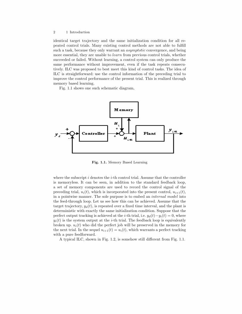
Fig. 1.1 shows one such schematic diagram,
Fig. 1.1. Memory Based Learning
where the subscript i denotes the i-th control trial. Assume that the controlleris memoryless. It can be seen, in addition to the standard feedback loop,a set of memory components are used to record the control signal of thepreceding trial, ui(t), which is incorporated into the present control, ui+1(t),in a pointwise manner. The sole purpose is to embed an internal model intothe feed-through loop. Let us see how this can be achieved. Assume that thetarget trajectory, yd(t), is repeated over a fixed time interval, and the plant isdeterministic with exactly the same initialization condition. Suppose that theperfect output tracking is achieved at the i-th trial, i.e. yd(t)−yi(t) = 0, whereyi(t) is the system output at the i-th trial. The feedback loop is equivalentlybroken up. ui(t) who did the perfect job will be preserved in the memory forthe next trial. In the sequel ui+1(t) = ui(t), which warrants a perfect trackingwith a pure feedforward.
A typical ILC, shown in Fig. 1.2, is somehow still different from Fig. 1.1.

1.1 What is Iterative Learning Control 3
Fig. 1.2. A typical ILC
The interesting idea is to further remove the time domain feedback fromthe current control loop. Inappropriately closing the loop may lead to insta-bility. To design an appropriate closed-loop controller, much of the processknowledge is required. Now suppose the process dynamics cannot escape toinfinity during the tracking period that is always a finite interval in ILC tasks.We need not even be bothered to design a stabilizing controller in the timedomain, as far as the control system converges gradually when the learningprocess repeats. In this way an ILC can be designed with the minimum systemknowledge.
In the field of ILC, such repeated learning trials are frequently describedby words like cycles, runs, iterations, repetitions, passes, etc. Since the ma-jority of ILC related work done hitherto is under the framework of contractionmapping characterized by an iterative process, it is thus more appropriate touse the words iteration(s), iteration axis, iteration domain, etc. to describesuch an iterative learning process, as we shall follow in the rest of this book.
The concept of performance improvement under a repeated operationprocess have long been observed, analyzed and applied [93] [129]. The ar-ticles by [7, 38, 9, 12, 64, 65] have formed the initial framework of ILC, underwhich subsequent developments have taken place over the years. Since then,though undergoing rapid progress, the main framework of ILC has been deter-mined and the majority of ILC schemes developed hitherto are still within thisframework, which is characterized by two key features: the linear pointwiseupdating law and iterative convergence, and is subject to two fundamentalconditions: the global Lipschitz continuity (GLC) condition and the identi-cal initialization condition (i.i.c). The contraction mapping methodology, amethod commonly used in function approximation and numerical analysis,has accordingly been brought up in iterative learning control design. In orderto capture the concept of ILC from a more quantified point of view, in therest of this section we shall conduct a rudimentary course briefing on ILC.

4 1 Introduction
1.1.1 The Simplest ILC: an example
To illustrate the underlying concepts and properties of ILC, let us start withthe simplest ILC problem: for a given process
y(t) = g(t)u(t)
where g(t) �= 0 is defined over a period [0, T ], find the control input, u(t),such that the target trajectory
yd(t) ∀t ∈ [0, T ]
can be perfectly tracked. Without loss of generality we assume that yd(t) andg(t) are bounded functions.
If g(t) is known a priori, this problem becomes a little trivial, as we cansimply calculate the desired control signal directly by inverting the process,which is exactly an open-loop approach
ud(t) =yd(t)g(t)
∀t ∈ [0, T ].
However, we know that any open-loop control schemes are sensitive to theplant modeling inaccuracy. In our case, if the exact values of g(t) are notavailable, the above simple open-loop scheme does not work. Let us assumethat g(t), though unknown, spans within 0 < α1 ≤ g(t) ≤ α2 <∞, where α1
and α2 are known lower and upper bounds. Can we find the desired controlprofile ud(t)? One may think of a two-stage approach. From the input-outputrelationship and the availability of the measurement of y(t) and u(t), firstidentify the time-varying gain g(t) point-wisely for t ∈ [0, T ]. Then the desiredcontrol signal can be computed according to the inverse relationship, ud(t) =yd(t)/g(t) ∀t ∈ [0, T ], provided that the function g(t) is captured perfectlyover [0, T ].
Can we merge the two stage control into one stage, that is, can we directlyacquire the desired control signal without any parametric or function identifi-cation? This will make the control system more efficient, and avoid extra errorincurred by any intermediate computation, e.g. a large numerical error mayoccur if g(t) takes a very small value at some instant t and is inverted. If thecontrol task runs once only and ends, we are not able to directly achieve thedesired control signal. When the same control task is repeated many times, wecan acquire the control signal iteratively by the following simplest iterativelearning control scheme
ui+1(t) = ui(t) + q∆yi(t) ∀t ∈ [0, T ] (1.1)
where the subscript i ∈ Z+ is the iteration index, Z+ = 0, 1, · · · is the set ofnon-negative integers. u0(t) can be either generated by any control method orsimply set to be zero. In fact all we need for u0(t) is to guarantee a bounded
1.1 What is Iterative Learning Control 5
output y0(t). q is a constant learning gain, and ∆yi(t)�= yd(t) − yi(t) is
the output tracking error sequence. Let us see how does this scheme workiteratively, and investigate conditions which ensure the system learnability.
First of all, we are going to execute the control action many times as ievolves, with the ultimate objective of finding out the desired control signal,ud(t), with respect to yd(t). Once yd(t) is given, ud(t) should be fixed. Thisimplies that the system, in this particular case the function g(t), defined over[0, T ], must be identical for any iterations. We know that a deterministicsystem will produce the same response when the same input repeats. Wethus define a repeatable control environment: a deterministic system with thecontrol task repeated over a fixed time interval. The repeatability is the veryfirst necessary condition for any deterministic learning controller to effectivelyperform.
Under the repeatable control environment, can the simplest ILC warrantsa convergence sequence of yi(t) to yd(t), or ui(t) to ud(t), as i → ∞? There
are two ways we can prove the convergence, either ∆yi(t) → 0, or ∆ui(t)�=
ud(i) − ui(t) → 0, when i→ ∞. For simplicity we will omit the time t for allvariables from 0 to T if not otherwise mentioned. First we demonstrate theconvergence of the output tracking sequence
∆yi+1 = yd − yi+1 = yd − gui+1 = yd − g(ui + q∆yi)= (yd − gui) − qg∆yi = (1 − qg)∆yi.
Consequently
|∆yi+1| ≤ |1 − qg| · |∆yi|.
On the other hand, we know 0 < α1 ≤ g(t) ≤ α2 < ∞, hence a conservativeselection of the learning gain is
q = α−12 .
It is easy to verify
0 ≤ |1 − qg| ≤ α2 − α1
α2= γ < 1
and
|∆yi+1||∆yi| ≤ γ < 1, ∀i ∈ Z+,
which shows
limi→∞
|∆yi| ≤ limi→∞
γi+1|∆y0| → 0
because y0(t) and yd(t) are finite in [0, T ].
6 1 Introduction
Now let us show, as an alternate way, that ∆ui → 0. Note
∆ui+1 = ud − ui+1 = ud − (ui + q∆yi)= (ud − ui) − q∆yi = ∆ui − q∆yi.
On the other hand,
∆yi = yd − yi = gud − gui = g∆ui.
By substituting ∆yi we have
∆ui+1 = (1 − qg)∆ui,
from which we can see that the convergence conditions are the same for thesequences ∆yi and ∆ui. In this particular problem, the convergence of ui toud implies the convergence of yi to yd. For more complicated problems relatedto the dynamic process or MIMO cases, they may show some differences.
Following the above demonstration on the simplest ILC, a question mayarise: does the simplest ILC still work if the process is nonlinear in controlinput u (non-affine-in-input)? In the following we will address this problem.
1.1.2 ILC for Non-affine Process
A non-affine-in-input process can be described by
y(t) = g(u(t), t) t ∈ [0, T ]
where g(u, t) is nonlinear in u, e.g. g = ueu. It is worth to point out that, evenif g is known a priori, the closed form of g−1 may not exist for most nonlinearfunctions. Thus we are not able to find the desired control profile by invertingthe process, consequently ud = g−1(yd(t), t) is not achievable. Moreover, inpractice g could be only partially known. To capture the desired control signal,we need to look for a more powerful approach, which is again the simplestILC (1.1) associated with certain condition imposed on the function g.
Let us first derive the convergence of the input sequence, ui → ud. Assumethat g is continuously differentiable to all the arguments, using the Mean ValueTheorem
∆yi = yd − yi = g(ud, t) − g(ui, t) = g(ud, t) − g(ud −∆ui, t)= g(ud, t) − [g(ud, t) − gu(ξi, t)∆ui] = gu(ξi, t)∆ui
where gu�= ∂f
∂u , and ξi ∈ [ud − |∆ui|, ud + |∆ui|]. Following the precedingderivation, and substituting the above relationship
∆ui+1 = ∆ui − q∆yi = ∆ui − qgu(ξi, t)∆ui
= (1 − qgu(ξi, t))∆ui,

1.1 What is Iterative Learning Control 7
hence
|∆ui+1| ≤ |1 − qgu(ξi, t)||∆ui|.In order to let |1 − qgu(ξi, t)| = γ < 1, the function g needs to meet thefollowing condition:
(C1) gu must have known lower and upper bounds, both are of the same signand strictly nonzero. Assume α1 the lower bound and α2 the upper bound,then either 0 < α1 ≤ α2 or 0 > α2 ≥ α1.
With this condition a learning gain q can be chosen to make γ strictly lessthan one. A conservative design is q = α−1
2 (for simplicity we only considerpositive gu). Note the similarity between the present non-affine and precedinglinear cases. gu is the equivalent process gain, like g(t) in the linear case, thusit naturally leads to the same convergence condition within the same boundingcondition. However, in the non-affine case the process gain gu is depending onthe control input u. Thus it is also necessary to limit u, especially when gu
turns out to be a radially unbounded function of u, i.e.
lim|u|→∞
|gu| → ∞.
In such circumstance we have to limit u to a compact set U . By virtue of thecontinuous differentiability of g, gu is bounded on U . For example considerg = ueu and u ∈ [0, um], then gu = eu+ueu, α1 = 1, and α2 = eum +ume
um <∞, as long as um is finite. Note that it is essential that, g �= 0 for the linearcases, or gu �= 0 for the non-affine cases, because the singularity yields a zeroprocess gain, hence the system is uncontrollable at the singular points.
Like the linear case, we can derive the same convergence property of theoutput sequence, yi → yd, as below
∆yi+1 = yd − yi+1 = g(ud, t) − g(ui+1, t) = g(ud, t) − g(ui + q∆yi, t)= g(ud, t) − g(ui, t) − gu(ξi, t)q∆yi = (1 − qgu(ξi, t))∆yi.
The convergence condition is the same: |1 − qgu(ξi, t)| = γ < 1.
1.1.3 ILC for Dynamic Process
Up to now the process discussed is static or memoryless. Now let us considerthe following SISO linear dynamics
x = ax+ bu x(0) = x0 (1.2)y = cx+ du
where a, b, c and d are unknown system parameters, either time-invariant ortime varying. Let us first focus on the time-invariant circumstance. If still using
8 1 Introduction
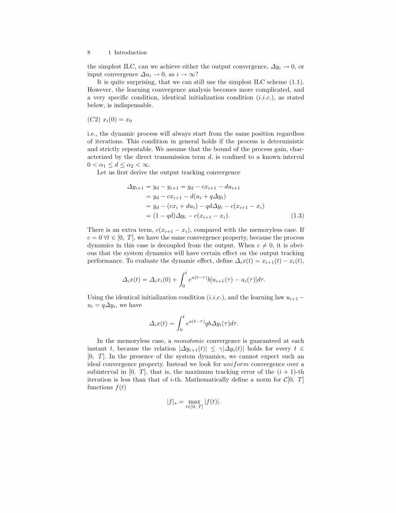
the simplest ILC, can we achieve either the output convergence, ∆yi → 0, orinput convergence ∆ui → 0, as i→ ∞?
It is quite surprising, that we can still use the simplest ILC scheme (1.1).However, the learning convergence analysis becomes more complicated, anda very specific condition, identical initialization condition (i.i.c.), as statedbelow, is indispensable.
(C2) xi(0) = x0
i.e., the dynamic process will always start from the same position regardlessof iterations. This condition in general holds if the process is deterministicand strictly repeatable. We assume that the bound of the process gain, char-acterized by the direct transmission term d, is confined to a known interval0 < α1 ≤ d ≤ α2 <∞.
Let us first derive the output tracking convergence
∆yi+1 = yd − yi+1 = yd − cxi+1 − dui+1
= yd − cxi+1 − d(ui + q∆yi)= yd − (cxi + dui) − qd∆yi − c(xi+1 − xi)= (1 − qd)∆yi − c(xi+1 − xi). (1.3)
There is an extra term, c(xi+1 − xi), compared with the memoryless case. Ifc = 0 ∀t ∈ [0, T ], we have the same convergence property, because the processdynamics in this case is decoupled from the output. When c �= 0, it is obvi-ous that the system dynamics will have certain effect on the output trackingperformance. To evaluate the dynamic effect, define ∆ix(t) = xi+1(t)− xi(t),
∆ix(t) = ∆ixi(0) +∫ t
0
ea(t−τ)b[ui+1(τ) − ui(τ)]dτ.
Using the identical initialization condition (i.i.c.), and the learning law ui+1−ui = q∆yi, we have
∆ix(t) =∫ t
0
ea(t−τ)qb∆yi(τ)dτ.
In the memoryless case, a monotonic convergence is guaranteed at eachinstant t, because the relation |∆yi+1(t)| ≤ γ|∆yi(t)| holds for every t ∈[0, T ]. In the presence of the system dynamics, we cannot expect such anideal convergence property. Instead we look for uniform convergence over asubinterval in [0, T ], that is, the maximum tracking error of the (i + 1)-thiteration is less than that of i-th. Mathematically define a norm for C[0, T ]functions f(t)
|f |s = maxt∈[0, T ]
|f(t)|.

1.1 What is Iterative Learning Control 9
Then the maximum tracking error of the i-th iteration is |∆yi|s. Now theupper bound of ∆ix can be evaluated
|∆ix|s ≤∫ t
0
ea(t−τ)|qb| |∆yi(τ)|sdτ
≤ |qb| |∆yi|s∫ T
0
e|a|(T−τ)dτ
≤ wi|∆yi|s (1.4)
where
wi�=
|qb|e|a|T − 1|a| a �= 0
|qb|T a = 0.
In the sequel, taking the norm | · |s in (1.3) and using (1.4), yields
|∆yi+1|s ≤ |1 − qd|s|∆yi|s + |c|wi|∆yi|s. (1.5)
Since we can always choose q such that |1 − qd|s ≤ γ < 1, there exists apositive constant δ satisfying γ+ δ < 1. It is easy to verify that if the trackinginterval [0, T1] ⊂ [0, T ], where T1 is given as
T1 ≤
1|a| ln
[1 +
δ|a||qcb|
]a �= 0
δ
|qcb| a = 0
(1.6)
then
|∆yi+1|s ≤ (γ + δ)|∆yi|s.As γ and δ are iteration independent, γ + δ < 1 ensures a geometric conver-gence of the output tracking error sequence.
From the above derivation procedure, it can be seen that the learningconvergence property in a dynamic process is quite different from a staticprocess:
1. ILC in a static process achieves monotonic convergence at each time t,whereas in a dynamics process only ensures monotonic convergence interms of the maximum error over a limited time interval. This is due tothe dynamic influence from ∆ix to ∆yi;
2. In the dynamic process, an extra i.i.c., ∆ix(0) = 0, is required. Thisis again due to the dynamic influence from ∆ix to ∆yi. The solutiontrajectory of a differential equation is determined by its initial value andexogenous input. If the initial value xi(0) varies at every iteration, it isno longer a strictly repeatable control environment;

10 1 Introduction
3. The time interval of the target trajectory, [0, T ], is limited by (1.6). In thestatic learning process we do not have such a limit. Note that the dynamicinfluence, quantified by (1.4) in the worst case, enters the convergencecondition (1.5) as a disturbance and increases as T increases. It can alsobe seen that the absolute value of the system parameter a is taken intoconsideration. Equivalently the dynamics is treated as a divergent one,even though the original a may take a negative value (stable). In orderto prevent the assumed divergent term ∆ix(t) from growing too largerand dominating the learning process, T1 must be sufficiently small. Thislimitation on T can be overcome by introducing a time-weighted norm (tobe addressed in next chapter).
Now let us derive the convergence conditions for the input sequence. Itrequires a different identical initialization condition
(C2′) xi(0) = xd(0),
i.e., the dynamic process will have to start from the same initial position asthe state trajectory xd(t) generated by ud(t). This condition is obviously morespecific than (C2). On the other hand, it provides certain convenience whenderiving the higher order ILC schemes, as can be seen in subsequent chapters.
Assume there exists a control input ud, which generates xd and yd, namely
xd = axd + bud xd(0) = x0
yd = cxd + dud.
Our objective is to show that the simplest ILC scheme (1.1) can converge tothe desired ud. First we can derive the relation
∆ui+1 = ud − ui+1 = ud − ui − q∆yi
= ∆ui − qc∆xi − qd∆ui
= (1 − qd)∆ui − qc∆xi (1.7)
where ∆xi�= xd − xi. The state error dynamics is
∆xi = xd − xi = a(xd − xi) + b(ud − ui)= a∆xi + b∆ui.
Integrating both sides of the state error dynamics and using the i.i.c. (C2′)yields
∆xi(t) = ∆xi(0) +∫ t
0
ea(t−τ)b∆ui(τ)dτ
=∫ t
0
ea(t−τ)b∆ui(τ)dτ.
The upper bound of the tracking error ∆xi(t), analogous to (1.4), is

1.1 What is Iterative Learning Control 11
|∆xi|s ≤ wi|∆ui|s.where
wi�=
|b|e|a|T − 1|a| a �= 0
|b|T a = 0.
Consequently from (1.7)
|∆ui+1|s ≤ |1 − qd|s|∆ui|s + |c|wi|∆ui|s. (1.8)
Note the analogy between the above formula and (1.5), the differences lie inthe replacement of ∆yi and wi by ∆ui and wi respectively. Thus the sameconvergence property can be derived: if the interval T is less than the limit(1.6), ui(t) converges uniformly to ud(t).
Though only a linear time-invariant (LTI) system is considered, the aboveresults can be easily extended to linear time-varying (LTV) systems with time-varying parameters a(t), b(t), c(t) and d(t). Assume d(t) ∈ [α1, α2] as before,and |a|s, |b|s, |c|s are finite, the only difference is the convergence interval
T1 ≤
1
|a|s ln[1 +
δ|a|s|c|s|b|s|q|
]a �= 0
δ
|c|s|b|s|q| a = 0.(1.9)
1.1.4 D-Type ILC for Dynamic Process
Often the following LTI dynamics is encountered in practice
x = ax+ bu x(0) = x0
y = cx
where the direct transmission term du is absent. From the system theory,we known that d �= 0 indicates a relative degree of zero, if d = 0 but cb �=0, the relative degree is one. Can we still apply the simplest ILC scheme(1.1) for systems without the direct transmission term d? From the precedingderivation (1.3), associated with the expression of ∆ix(t), and setting d = 0,we have
∆yi+1(t) = ∆yi(t) −∫ t
0
ea(t−τ)qb∆yi(τ)dτ.
The integral term may be either positive or negative, depending on the entirehistory of ∆yi(τ) ∀τ ∈ [0, t]. As a consequence, there is no guarantee that theabsolute value of the right hand side can be made less than that of the lefthand side, no matter how to select the learning gain, q.
12 1 Introduction
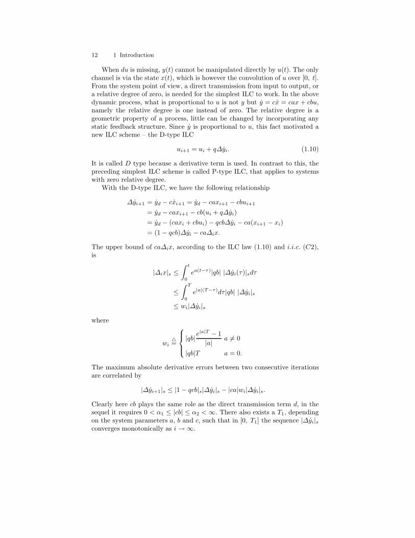
When du is missing, y(t) cannot be manipulated directly by u(t). The onlychannel is via the state x(t), which is however the convolution of u over [0, t].From the system point of view, a direct transmission from input to output, ora relative degree of zero, is needed for the simplest ILC to work. In the abovedynamic process, what is proportional to u is not y but y = cx = cax + cbu,namely the relative degree is one instead of zero. The relative degree is ageometric property of a process, little can be changed by incorporating anystatic feedback structure. Since y is proportional to u, this fact motivated anew ILC scheme – the D-type ILC
ui+1 = ui + q∆yi. (1.10)
It is called D type because a derivative term is used. In contrast to this, thepreceding simplest ILC scheme is called P-type ILC, that applies to systemswith zero relative degree.
With the D-type ILC, we have the following relationship
∆yi+1 = yd − cxi+1 = yd − caxi+1 − cbui+1
= yd − caxi+1 − cb(ui + q∆yi)= yd − (caxi + cbui) − qcb∆yi − ca(xi+1 − xi)= (1 − qcb)∆yi − ca∆ix.
The upper bound of ca∆ix, according to the ILC law (1.10) and i.i.c. (C2),is
|∆ix|s ≤∫ t
0
ea(t−τ)|qb| |∆yi(τ)|sdτ
≤∫ T
0
e|a|(T−τ)dτ |qb| |∆yi|s≤ wi|∆yi|s
where
wi�=
|qb|e|a|T − 1|a| a �= 0
|qb|T a = 0.
The maximum absolute derivative errors between two consecutive iterationsare correlated by
|∆yi+1|s ≤ |1 − qcb|s|∆yi|s − |ca|wi|∆yi|s.Clearly here cb plays the same role as the direct transmission term d, in thesequel it requires 0 < α1 ≤ |cb| ≤ α2 < ∞. There also exists a T1, dependingon the system parameters a, b and c, such that in [0, T1] the sequence |∆yi|sconverges monotonically as i→ ∞.

1.1 What is Iterative Learning Control 13
A concern towards the D-type ILC is the demand on the derivative signals.In control theory and control practice, the availability of derivative signals ofthe system states is out of the question. However, this problem does not arisein the D-type ILC, simply because the derivative signals used for the presentiteration are from the previous iteration. Therefore, one may use various kindsof filters, such as non-causal or zero-phase filters, to generate the derivativesignals from the past output measurement.
So far we only prove the convergence property of the error derivative. Inorder to get the error convergence, we need one more identical initializationcondition.
(C2′′) ∆yi(0) = yd(0) − yi(0) = 0,
indeed, from∆yi(t) = 0 and∆yi(0) = 0 as i→ ∞, we have∆yi(t) = ∆yi(0) =0 ∀t ∈ [0, T ].
Likewise we can derive the convergence property of ∆ui associated withthe i.i.c. (C2′) and (C2′′). The results can also be extended to LTV systems.
1.1.5 Can We Relax the Identical Initialization Condition?
As shown in the previous analysis, the identical initialization conditions (C2),(C2′) and (C2′′) play the key role in ILC. The identical initialization condition,together with the global Lipschitz continuity condition, are two fundamentalassumptions of ILC. A frequently raised question is, can i.i.c. be relaxed orremoved? The i.i.c. have been criticized by control experts from differentdisciplines. Indeed, there are real systems well equipped with almost perfecthoming mechanism such as high precision XY-table, robotic manipulatorson assembly line, etc. However, for many practical control problems, perfectinitialization is hardly achievable.
This issue has been exploited by many researchers [71, 103, 104, 53, 72,100, 132], etc. The results confirm that i.i.c. are really imperative, and anysmall discrepancy in the initial value may lead to a divergent sequence. Thereason is simple: the ILC algorithms, such as (1.1) and (1.10), are integratorsalong the iteration axis, which will accumulate any biased signals. Let us lookat the simplest ILC law (1.1), and assume a small initial discrepancy in oneof the i.i.c., (C2′′),
∆yi(0) = yd(0) − yi(0) = ε, ∀i ∈ Z+
where 0 < ε 1 is a constant. Due to the integral nature of ILC in iterationdomain, at t = 0
ui+1(0) = ui(0) + q∆yi(0)= ui−1(0) + q∆yi−1(0) + q∆yi(0)
= · · · = u0(0) + qi∑
j=0
∆yj(0)

14 1 Introduction
= u0(0) + (i+ 1)qε (1.11)
which goes to infinity as the iteration number i → ∞. In this example, weassume the initial error sequence |∆yi(0)| ∈ l∞. The problem can be mitigatedto certain extent, if the initial error sequence is in l1. Further, if |∆yi(0)| is adiscrete-time zero mean white noise, then the mean value of ui(0) will convergeto zero.
To avoid the worst case of divergence, a well adopted remedy is to adda forgetting factor to the past control signal, and the simplest ILC (1.1), forinstance, becomes
ui+1(t) = pui(t) + q∆yi(t) ∀t ∈ [0, T ] (1.12)
where 0 < p ≤ 1 is the forgetting factor. Obviously, p = 1 corresponds to theintegral action, and 0 < p < 1 corresponds to a low pass filter in the iterationdomain. The trade-off is, the learned useful signal will also be discounted.Recently two works relevant to i.i.c. have been reported. In [26], an initialstate learning algorithm has been proposed to address the first i.i.c., (C2), bymaking the initial state xi(0) a convergent sequence. The price is, one needsto assume that the system states, at least the initial states, are accessible andreachable. In [124], an initial rectifying action is proposed to address the i.i.c.(C2′′), by revising the target trajectory nearby the initial stage into a newone, which aligns its initial value with that of the actual system output.
Generally speaking, i.i.c. and GLC are necessary within the present ILCframework based on contraction mapping. In order to remove those conditions,we have to establish a new learning control framework.
1.1.6 Why ILC
From the above descriptions, though extremely simple, we can see the featuresof ILC:
1. ILC aims at output tracking control, without using any knowledge of thesystem state;
2. It has a very simple structure – an integration along the iteration axis;3. It is a memory based learning process, as we need to record error signals∆yi(t) and control input signals ui(t) over the entire time interval [0, T ];
4. It is open-loop in the time domain, but closed − loop in the iterationdomain. The present control input consists of error and input signals ofthe previous iteration only;
5. It requires very little system knowledge, in fact only the bound of thedirect tranmission term, for instance the parameter d, is needed to guar-antee the learning convergence iteratively. Thus it is almost a model-freemethod. This is a very desirable feature in control implementation;
6. Due to the open-loop nature, there is no warranty of the stability of thedynamic system along the time axis. As far as the interval T is finite, and
1.1 What is Iterative Learning Control 15
the dynamics is either linear or GLC, finite escape time phenomenon doesnot occur, hence the system state is always bounded. We will discuss thisin more details in Chapter 7;
7. The i.i.c. (C2), (C2′) and (C2′′) play important role in the learningprocess;
8. The control task – the target trajectory yd(t) must be identical for alliterations.
We can see, that ILC complements existing control approaches in manyaspects, and offers an alternative way to handle uncertain systems. One mayargue, that for such a simple LTI or LTV system as (1.2), many other controlmethods are also applicable and able to achieve equally good performance. Letus consider a simple case, where a(t) in (1.2) is an unknown and rapid timevarying parameter. Since a(t) is unknown to us, we have to assume the worstcase that it may take any positive value (open-loop unstable). Consequentlywe need to close the loop with a sufficiently high gain, which leads to a veryconservative control design, even though a(t) may actually be negative ∀t ∈[0, T ], i.e. the system is open-loop stable. On the contrary, ILC offers alow gain control, which is able to learn and improve the control performanceiteratively. We can verify this property from the preceding ILC design, wherethe learning gain q is always chosen to be sufficient low.
Let us consider another example
x = f(x, u, t) x(0) = x0
y = g(x, u, t)
where f and g are global Lipschitz continuous functions of the argumentsx and u. As we will demonstrate later in Chapters 2 to 6, the only priorinformation required in ILC design, is
∂g
∂u∈ [α1, α2] ∀x, u, t.
This prior information, however, is inadequate for us to complete the designby means of many existing control methods.
It is natural for control experts to raise another question, that it wouldbe practically ill-logical to totally ignore the dynamics f(x, u, t) if we do havepartial knowledge, for instance, f(x, u, t) may consist of a nominal part, and aparametric or non-parametric uncertain component. Indeed, the best controlmethod should be the one fully using all available information. From Chapters7 to 9, we shall show a new ILC framework, which allows us to incorporate allthe system information, and further integrate both nonlinear feedback controland memory based nonlinear learning control.
16 1 Introduction
1.2 History of ILC
Various ILC schemes have been proposed in the past two decades. The be-ginning work [8], focused on the output tracking, first formulated the P -typeand D-type ILC schemes with convergence analysis. Since then, ILC has beenextensively studied and achieved significant progress in both theory and ap-plications, and now becomes one of the most active fields in intelligent controland system control. In the history of ILC development, theory, design and ap-plications have been widely exploited. We summerize briefly the developmentof ILC in the following aspects.Contraction Mapping MethodContraction mapping method forms the basis of ILC theory. All preceding ILCdesign examples can be regarded as the simple form of contraction mapping,though without rigorous mathematical derivations. The key requirements ofsuch kind of method are the global Lipschitz continuity (GLC) of systemdynamics, as well as the identical initialization condition. The perfect outputtracking can be achieved in any finite time interval, by means of the time-weighted norm. Along the direction of [8, 10], P-type ILC [14, 113, 111, 33, 27],D-type ILC [8, 51, 53], PD-type ILC [74], high-order ILC [17, 24, 28, 27, 23],etc. have been reported.
Note that the ILC mechanism, such as (1.1) and (1.10), links the sys-tem dynamics between two consecutive iterations, hence generates a dis-crete dynamics along iteration axis. The learning performance analysis hasbeen conducted in the iteration domain, by [77, 6, 118, 69, 16, 142, 148],etc., and in particular the robustness of ILC has also been investigated by[13, 14, 24, 113, 33, 72, 118, 144, 74, 27, 148], etc.
ILC has been extended to miscellaneous systems, including time-delaysystems [55, 109, 100, 59, 139], sampled-data systems [138, 32], discrete-timesystems [127, 49, 68, 128, 3, 6, 112, 31, 28, 131, 60] and distributed parametersystems [79, 106], etc.
Design and analysis of ILC in the frequency domain has attracted equalattention as in the time domain, see [54, 58, 43, 81, 78, 42, 59, 140], etc.The frequency analysis plays a crucial role in ILC applications, because theconvergence condition can be relaxed from the infinite frequency bandwidthto a finite frequency bandwidth. ILC with H∞ design [96, 5, 40], ILC withoptimal design [4, 46, 70], etc. have also been exploited.2-D Theory Based Method2-D system theory [19, 108, 112, 110] considers the time domain and the iter-ation domain simultaneously. Taking advantage of the advanced linear multi-variable theory, the convergence of the tracking error in iteration domain andstability in time-domain can be analyzed systematically. ILC designs basedon Linear 2-D theory 2-D theory have been explored [49, 68, 2, 35, 44], etc.Nonlinear 2-D theory has also been exploited [67].Energy Function MethodLyapunov’s direct method has been widely employed in the control design and

1.3 Book Overview 17
analysis of nonlinear dynamic systems, and now regarded as one of the mostimportant tools in dealing with nonlinear uncertain systems. Being inspiredby Lyapunov’s direct method, the concept of energy function in both thetime domain and the iteration domain has been developed, which opens anew avenue for the learning control design and convergence analysis in theiteration domain.
ILC based on an energy function defined in the iteration domain havebeen developed [50, 97, 144]. With the help of this approach, robust learningcontrol [63, 143, 135] and adaptive learning control [82, 66, 94, 62, 122, 134]have been developed to handle nonlinear systems with parametric or non-parametric uncertainties.
Recently the composite energy function (CEF), which reflects the systemenergy in both the time domain and the iteration domain, is further devel-oped and applied to ILC [145, 147], etc. By means of energy function, thenew and powerful control design methods, such as the backstepping designand nonlinear optimality, can be used as systematic design tools for the ILCconstruction [47, 146, 107].ApplicationsBesides the theoretical development, ILC schemes have been applied to manypractical control engineering problems. One of the main application areas isrobotic control, for instance, the rigid robotic manipulators [11, 150, 15, 91],robotic manipulators with flexible joints [130], and flexible links [79], etc. ILChas also been applied to a variety of real-time control problems. Here weonly select a subset from the application list: batch process [73, 139], wafertemperature control [34], welding process [86], disk drives [83, 30], hydraulicservo [99], piezoelectronic motor [126], PMS motor [141], linear motor [125],switched reluctance motor [114], injection molding machine [52], functionalneuromuscular stimulation [41], aero-related problems [29], etc. A number ofpractical ILC design guidelines have been summarized, e.g. [75, 76], etc.Supplementary Literature SurveyAmong the numerous ILC publications, there are a number of publicationsoffering wide survey on the state-of-the-art progress in the ILC field, includ-ing [88, 85, 136, 132, 133], etc. Besides, two monographs [84, 25], one editedvolume [18] and two special issues [36, 37] summarized the latest ILC devel-opments and achievements respectively, by the time of publication.
1.3 Book Overview
The contents of the book can be roughly categorized into two parts. The firstpart of this book, from Chapters 2 to 6, focuses on ILC design and analysisunder the framework of contraction mapping. The dynamic systems underconsideration are essentially linear or global Lipschitz continuous. The ILC isto perform the output tracking tasks. As far as the learning algorithms areconcerned, the first part can be further divided into the linear ILC (Chapters

18 1 Introduction
2-4) and nonlinear ILC (Chapters 5-6). The second part of this book, fromChapters 7 to 9, concentrates on ILC based on the composite energy function.The dynamic systems under consideration can be local Lipschitz continuousand associated with either time-varying parametric or non-parametric uncer-tainties. The ILC is to perform tracking control in the state space.
Distinct from most control methods, ILC permits an extra degree of free-dom – learning along the iteration axis. This new property, however, also givesrise to a new challenge – how to quantify and evaluate the performance of ILCin the iteration domain? Second, with the only available system knowledgeregarding the interval bound of the system gain, can we still design an ILC insome optimal sense? Chapter 2 addresses those two issues. First, three perfor-mance indices – convergence speed, the global uniform bound of the learningerror in the iteration domain, and the monotonic convergence interval – havebeen introduced to quantify and evaluate the learning performance in the iter-ation domain. Then a new robust optimal design, based on the interval boundof the system gain, is developed for linear ILC schemes to achieve the fastestlearning convergence speed.
Most ILC schemes use the control information acquired in the previousiteration. One question is: why not use the control information of more thanone iteration? Intuitively, the more information can an ILC use, the betterwould be the learning performance. This is a rather controversial issue in ILCarea. In Chapter 3 we show that this intuition may not be true, as far as theconvergence speed under the interval uncertainty is concerned. The simplestfirst order linear ILC, such as (1.1), could be the best.
The robust optimal design of linear-type ILC, presented in Chapter 2, isextended to MIMO systems in Chapter 4. The main difficulty of such extensionlies in the process of solving a min-max problem, where the system gain matrixunder consideration could be highly nonlinear, time-varying, uncertain, andasymmetric. An interesting method is developed in Chapter 4, which providesa new mathematical tool solving the min-max problem in general, and therobust optimal ILC design in particular.
In practice, the learning speed along the iteration axis is the most impor-tant factor. A question immediately following the Chapter 3 is, can we comeup with an ILC scheme with a faster convergence speed than the simplest firstorder linear ILC? Chapter 5 provides the answer – a conditional yes, if weare allowed to use the system state information, and the output relation, i.e.y = g(x, u, t), is completely known to us. Two types of nonlinear ILC schemes– the Newton-type and Secant-type, are developed. It is shown by rigorousproof, that the Newton-type ILC achieves the fastest convergence speed, andthe Secant-type ILC wins the second place.
In Chapter 6, the nonlinear ILC schemes, the Newton-type and Secant-type, are extended to MIMO systems.
Upto Chapter 6, all ILC schemes focus on GLC systems with output track-ing, in an almost model free manner, at most only use the output relation.Can the iterative learning be extended to more general classes of nonlinear
1.3 Book Overview 19
systems? Can an iterative learning controller incorporate more of system statedynamics knowledge if it is available? Chapter 7 attempts to establish such aframework based on the composite energy function (CEF). The CEF consistsof two components: one is a positive scalar function capturing the trackingerror information in the time domain, and the other is a functional over theentire learning period reflecting the (parametric) learning error in the iterationdomain. When the system unknowns are limited to time-varying parameters,it is easy to construct an nonlinear learning mechanism, consisting of a non-linear stabilizing feedback part and a pointwise learning part. The bottleneckin contraction mapping based ILC, the GLC assumption, can thus be over-come.
One important contribution of CEF is, it bridges the gap between ILCand other advanced nonlinear control methods, such as nonlinear optimal con-trol, nonlinear internal model control, adaptive control, nonlinearH∞ control,nonlinear robust control, etc. Chapter 8 demonstrates one such integration –quasi-optimal ILC, based on a modified Sontag’s formula for the known nomi-nal part of the process. Meanwhile, learning is carried out iteratively to handletime-varying uncertainties in the nonlinear dynamic system. Along with thepointwise convergence in learning, the suboptimal properties, such as the bal-ance between the control effort and the tracking error in the iteration domain,are preserved.
Finally we explore another important direction: combination of ILC andother predominant intelligent control methods characterized by black-boxbased approximations. By virtue of the CEF based design, Chapter 9 ex-ploits a learning wavelet control method to achieve the pre-defined trackingperformance in finite iterations and ensure the boundedness of all signals.Different from other intelligent control methods such as neural control, thenovelty of the learning wavelet control lies in that both the network parame-ters and structure can be tuned easily, owing to the orthonormality propertyof the wavelet network. Further, by virtue of the multi-resolution property ofthe wavelet network, the finiteness of the network structure is assured. Thelearning wavelet control mechanism can successfully handle the lumped (non-parametric) system uncertainties, for instance the L2(R) class in the statespace.
Conclusions are drawn and some recommendations for future research aregiven in Chapter 10. [1, 2]


