Measure of bullwhip effect considering stochastic disturbance based on price fluctuations in a supply chain with two retailers JUNHAI MA Tianjin University College of Management and Economics Tianjin 300072 CHINA [email protected]JING ZHANG Tianjin University College of Management and Economics Tianjin 300072 CHINA [email protected]Abstract: This paper establishes a new price-sensitive demand model which considers stochastic disturbance simi- lar to ARMA(1,1) model. We examine the impact of two forecasting methods on the bullwhip effect in a two-stage supply chain with two retailers. It is assumed that two retailers face the same demand model and an order-up-to inventory policy is employed. The lead-time demand is forecasted respectively by the moving average (MA) and exponential smoothing(ES) methods. The effect of various parameters is investigated by numerical simulation and the bullwhip effect under two forecasting methods is compared. The results show that the MA forecasting method is better than the ES method based on our demand process. Besides, conclusions indicate that both the extent of consumers concerning about the historical price volatility and the lead time play significant roles on reducing the bullwhip effect, and stochastic disturbance impacts the bullwhip effect differently based on the lead time. The larger the variance of stochastic disturbance of the retailer which has a longer lead time, the greater the bullwhip effect in the supply chain. The moving average coefficient of stochastic disturbance generally has a little different impact on the bullwhip effect under the different relationship of the lead time between two retailers. Moreover, some proposals are present to help managers to take appropriate measures and select the forecasting method that yields the lowest bullwhip effect. Key–Words: Supply chain, Bullwhip effect, Demand forecasting, Price fluctuations, Stochastic disturbance 1 Introduction For many companies, bullwhip effect is a high-risk phenomenon prevalent in their marketing activities, and has serious impacts on operational costs. With its influence on integrating business activities, bullwhip effect has become a focus in supply chain manage- ment research, attracting the attention of researchers and practitioners. It refers to the empirical and the- oretical observation that as moving up from a down- stream member to an upstream member, the demand variability placed by the downstream member to its (immediate) upstream member tends to be amplified in a supply chain. The first evidence of this phenomenon can be traced back to Forrester (1958, 1961) who discov- ered its causes and possible remediation in the con- text of industrial dynamics. After that, many re- searchers also acknowledged the existence of the bull- whip effect in supply chains, such as Blinder (1982), Blanchard (1983), Burbidge (1984), Caplin (1985), Blinder (1986) and Kahn (1987). Then, a well- known classic beer game which has been used in busi- ness schools for decades is experimented by Sterman (1989) to illustrate the bullwhip effect. The bullwhip effect is first named by Lee et al. (1997a, b), whose works is the milestone for the research of bullwhip effect, who identified that demand signal processing, non-zero lead time, supply shortage, order batching, and price fluctuation are the five main causes of the bullwhip effect in supply chains. Base on Lee et al. (1997a, b), the bullwhip effect may be mitigated by eliminating its main causes. With various causes of the bullwhip effect, the demand pro- cess and forecasting methods are considered most fre- quently because they directly affected the inventory system of supply chains. Different demand processes and different forecasting methods are employed in a lot of papers. Lee et al. (2000) followed a first-order autore- gressive process and a simple order-up-to inventory policy with a minimum mean square error (MMSE) forecasting technique measuring the benefit of infor- mation sharing between a retailer and a manufacturer in a two-stage supply chain. Using a first-order au- toregressive (AR(1)) demand process similar to Lee et al. ( 1997a, b), Chen et al. (2000a,b) investigat- WSEAS TRANSACTIONS on MATHEMATICS Junhai Ma, Jing Zhang E-ISSN: 2224-2880 127 Volume 14, 2015
Transcript
Measure of bullwhip effect considering stochastic disturbancebased on price fluctuations in a supply chain with two retailers
Abstract: This paper establishes a new price-sensitive demand model which considers stochastic disturbance simi-lar to ARMA(1,1) model. We examine the impact of two forecasting methods on the bullwhip effect in a two-stagesupply chain with two retailers. It is assumed that two retailers face the same demand model and an order-up-toinventory policy is employed. The lead-time demand is forecasted respectively by the moving average (MA) andexponential smoothing(ES) methods. The effect of various parameters is investigated by numerical simulation andthe bullwhip effect under two forecasting methods is compared. The results show that the MA forecasting methodis better than the ES method based on our demand process. Besides, conclusions indicate that both the extent ofconsumers concerning about the historical price volatility and the lead time play significant roles on reducing thebullwhip effect, and stochastic disturbance impacts the bullwhip effect differently based on the lead time. Thelarger the variance of stochastic disturbance of the retailer which has a longer lead time, the greater the bullwhipeffect in the supply chain. The moving average coefficient of stochastic disturbance generally has a little differentimpact on the bullwhip effect under the different relationship of the lead time between two retailers. Moreover,some proposals are present to help managers to take appropriate measures and select the forecasting method thatyields the lowest bullwhip effect.
1 IntroductionFor many companies, bullwhip effect is a high-riskphenomenon prevalent in their marketing activities,and has serious impacts on operational costs. With itsinfluence on integrating business activities, bullwhipeffect has become a focus in supply chain manage-ment research, attracting the attention of researchersand practitioners. It refers to the empirical and the-oretical observation that as moving up from a down-stream member to an upstream member, the demandvariability placed by the downstream member to its(immediate) upstream member tends to be amplifiedin a supply chain.
The first evidence of this phenomenon can betraced back to Forrester (1958, 1961) who discov-ered its causes and possible remediation in the con-text of industrial dynamics. After that, many re-searchers also acknowledged the existence of the bull-whip effect in supply chains, such as Blinder (1982),Blanchard (1983), Burbidge (1984), Caplin (1985),Blinder (1986) and Kahn (1987). Then, a well-known classic beer game which has been used in busi-ness schools for decades is experimented by Sterman
(1989) to illustrate the bullwhip effect. The bullwhipeffect is first named by Lee et al. (1997a, b), whoseworks is the milestone for the research of bullwhipeffect, who identified that demand signal processing,non-zero lead time, supply shortage, order batching,and price fluctuation are the five main causes of thebullwhip effect in supply chains.
Base on Lee et al. (1997a, b), the bullwhip effectmay be mitigated by eliminating its main causes. Withvarious causes of the bullwhip effect, the demand pro-cess and forecasting methods are considered most fre-quently because they directly affected the inventorysystem of supply chains. Different demand processesand different forecasting methods are employed in alot of papers.
Lee et al. (2000) followed a first-order autore-gressive process and a simple order-up-to inventorypolicy with a minimum mean square error (MMSE)forecasting technique measuring the benefit of infor-mation sharing between a retailer and a manufacturerin a two-stage supply chain. Using a first-order au-toregressive (AR(1)) demand process similar to Leeet al. ( 1997a, b), Chen et al. (2000a,b) investigat-
WSEAS TRANSACTIONS on MATHEMATICS Junhai Ma, Jing Zhang
E-ISSN: 2224-2880 127 Volume 14, 2015
ed the impact of the simple moving average(MA) andexponential smoothing(ES) forecasts on the bullwhipeffect for a simple, two-stage supply chain with onesupplier and one retailer. Likewise, Zhang (2004) alsoused an AR(1) demand process to investigate the im-pact of different forecasting methods on the bullwhipeffect. Luong (2007) measured the bullwhip effect ina simple supply chain including one retailer and onesupplier by performing the AR(1) demand forecastingprocess on the base stock policy for their inventoryunder the MMSE forecasting technique. As a sequelof Luong (2007), Luong and Phien(2007) investigat-ed autoregressive models with higher order, first han-dling AR(2) demand process and considering the gen-eral AR(p) demand process with the MMSE method.By quantifying the bullwhip effect, all the above pa-pers using an AR(1) process, investigated the behav-ior of autoregressive coefficients and order lead-timeand showed effects of different forecasting method-s on bullwhip effect measures. Moreover, Duc et al.(2010) continued using AR(1) process to examine theeffect of a third-party warehouse on the bullwhip ef-fect and inventory cost in a three-stage supply chainwith a supplier ,a third-party warehouse and two re-tailers.
Note that several academics (Lee et al. (1997a,b),Chen et al. (2000 a,b), Xu et al. (2001), Zhang(2004) et al.) assumed a pure autoregressive pro-cess and Graves (1999) assumed a pure moving av-erage process. However, the demand model seldomhas characteristics of a pure autoregressive processor a pure moving average process. While the de-mand process usually has characteristics of both mov-ing average and autoregressive process, Pindyck et al.(1998) proposed that a mixed autoregressive-movingaverage (ARMA) demand process is more suitable forthe time series of the market demand than the ARmodel. Subsequently, the ARMA model is frequentlyused. Disney et al.(2006) quantified the bullwhip ef-fect for the mixed first-order autoregressive-movingaverage(ARMA(1,1)) demand pattern under the ESforecasting method in a single supply chain echelonwith the base stock policy for replenishment. Ducet al.(2008) investigated the impact of the autoregres-sive coefficient, the moving average parameter, andthe lead time on the bullwhip effect via a ARMA(1,1)model when the demand forecast is performed by theMMSE method. Likewise, by using the dynamic sim-ulation, Feng (2008) evaluated the different effects ofthree forecasting methods, i.e., MA, ES and MMSEmethods, for the simple supply with an ARMA(1,1)model chain as is done in the research of Disney etal. (2006). As an extension of Feng (2008), Ma(2013)made a new supply chain with one supplier and tworetailers who both employ the ARMA(1,1) demand
process, and analyzed and compared the impact ofparameters on the bullwhip effect under various fore-casting methods. As a further development of ARMAmodel, Gilbert(2005) used a new Autoregressive Inte-grated Moving Average (ARIMA) time-series modelto present the causes of the bullwhip effect and man-agerial insights about reducing the bullwhip effect in amultistage supply chain model. Based on the ARIMAdemand pattern, Dhahri (2007) alleviated the bullwhipeffect in two respects-namely increase of the stocklevel and reduction of the service given back to cus-tomers.Claudimar(2014) also used ARIMA model fordemand forecasting in the food retail.
Performance of a supply chain is affected not on-ly by demand forecasting but also by price fluctua-tion. The price has an important effect on the demandvariability. However, while many researchers explorethe demand process, inventory policy and forecast-ing technique, seldom papers consider price in thedemand process. However, in other supply chain re-search, kinds of price-demand models are used, suchas many recent papers: Junhai Ma(2014), Lei X-ie(2014), Fang Wu(2014) and Lisha Wang(2014). Re-fer to these price models and classic cournot model,prices can be added into the demand process for s-tudying the influence on the bullwhip effect. Hamis-ter et al.(2008) improved the first-order autoregressiveand considered the effect of current prices on the de-mand based on the correlation with the previous de-mand. Rong et al.(2009) put forward that the demandis not only affected by the current price, but also by theprevious period of price, for analyzing the impact ofprice fluctuation and consumer response on the sup-ply chain in the supply disruptions. Furthermore, anonlinear demand process about retail price was es-tablished by Ma et al. (2008) and this paper studiedretailer’s demand decision and the complex behaviorbetween the retailer and the whole supply chain. Re-cently, Ma et al.(2012a) established a price-sensitivelinear demand model by considering the current priceand the one period-ahead price in a two-stage supplychain with one supplier and one retailer, and analyzedthe impact of price forecasting behavior by consumer-s on the BWE and inventory level. In a sequel, Ma etal.(2012b) extended the research to the case in whichn period-ahead price is used in the demand process toinvestigate the impact of price forecast, furthermore,extended their results to multiple retailers and derivedthe analytical total order quantity.
This paper continues to study the price-sensitivedemand process on the impact of bullwhip effect. Inthe current research, we will quantify the bullwhipeffect in a two-stage supply chain with one supplierand two retailers on a price-sensitive demand process.Furthermore, a measure of the bullwhip effect will
WSEAS TRANSACTIONS on MATHEMATICS Junhai Ma, Jing Zhang
E-ISSN: 2224-2880 128 Volume 14, 2015
be developed under the simple ES and MA forecast-ing technique, based on a replenishment model whichis similar to the one used by Chen et al. (2000a,b).Meanwhile the retailers both employ the base stockpolicy for replenishment. We also analyze the impactof parameters on the BWE under the MA and ES fore-casting methods and compare the different effect oftwo methods on the bullwhip effect.
Our paper differs from the previous research inthe following ways. First, we develop a new demandprocess in which we add the first-order moving av-erage random disturbance into the price-sensitive de-mand model used in the work of Ma et al. (2012b),in order to evaluate the impact of price fluctuation andthe random disturbance parameter on the bullwhip ef-fect. Second, the current research aims at determin-ing an exact measure of the bullwhip effect in a sup-ply chain with one supplier and two retailers, which iscloser to the actual situation, while Ma et al.( 2012a,b) mainly developed a bullwhip effect measure for asimple two-stage supply chain with one supplier andone retailer only.
The remaining part of this paper is organized asfollows. In section 2, we present the stationary prop-erty of the new price-sensitive demand process in anew supply chain with one supplier and two retailer-s which both employ the order-up-to inventory poli-cy. In section 3, we quantify the bullwhip effect un-der MA and ES forecasting methods and derive theexpression of important parameters such as lead-timedemand forecast and variance of lead-time demandforecast error. We investigate its behavior and discussthe effects of parameters on the bullwhip effect underdifferent forecasting methods, then, compare the im-pact of two forecasting methods on the bullwhip effectin section 4. Finally, a short summary is concluded forthis paper in section 5. Proofs for some expressions inthis paper are summarized in the Appendix.
2 Supply chain modelThis research is conducted in two stages with one sup-plier and two retailers(see Figure.1). In the paper, weassume that our two retailers are in a duopolistic com-petitive industry. The two retailers face the customerdemands which consider price in a ARMA(1,1) pro-cess, and place orders to the supplier respectively. Thenew supply chain model is presented in this section.
2.1 Demand processThe demand forecast is performed through AR(p)(Leeet al., 1997a,b; Chen et al., 2000a,b; Zhang, 2004;Duc, 2010),ARMA(1,1) (Duc, 2008; Feng, 2008; Ma,2013) and ARIMA(Gilbert, 2005; Dhahri, 2007) in
Customer
Retailer 1
Retailer 2
Supplier
td
1,td
2,td2,tq
1,tq
tq
Figure 1: Two-stage supply chain model
most research which dont consider pricing .However,in our paper, demand is contingent on price and pricevolatility has great impacts on the demand.Only con-sidering current price, we can get price-sensitive de-mand function model:dt = a − bpt. In fact, pricevolatility may cause consumers to purchase in ad-vance. Similar to the customer behavior of MaY.G.etal.(2012),we also emphasize on the impact of cur-rent and previous prices of the demand based on theautoregressive-moving average model. We add s-tochastic disturbance into the demand model.Retailersorder and replenish their stock from a supplier on afixed time interval to supply customer demand. Allshortages are backordered.
Consider retailer 1 facing demand of the form
d1,t = a− bp1,t + rb(p1,t −n∑i=1
p1,t−i/n)
+ ε1,t − θ1ε1,t−1
(1)
Here,d1,t represents unit demand in the period t,which is linearly decreasing in price. p1,t is the mar-ket price during period t, which is independent andidentically distributed random variables.a is the mar-ket demand scale and b is a price sensitive coefficient,where a > 0, b > 0. r is the extent of customer con-cern about historical price volatility. The assumptionof 0 ≤ r < 1 assures that the negative impact of priceduring period t still dominates on the demand in theperiod t. When r = 0, the market demand is onlyrelated with the price in period t, ignoring the impactof the price-prediction behavior of consumers on de-mand under price fluctuation. ε1,t is independent andidentically distributed from a normal distribution withmean 0 and variance σ12. θ1 is the first-order movingaverage coefficient of retailer 1, where −1 < θ1 < 1.n is the span of previous prices for the demand model.
For the demand process to be stationary, we musthave
E(d1,t) = E(d1,t−1) = E(d1), ∀t
WSEAS TRANSACTIONS on MATHEMATICS Junhai Ma, Jing Zhang
E-ISSN: 2224-2880 129 Volume 14, 2015
Hence, a stationary condition can be given as
E(d1) = a− bE(p1,t) + rb(E(p1,t)
−n∑i=1
E(p1,t−i)/n).
In this paper, we assume
E(p1,t) = E(p1,t−1) = E(p1),∀t
and then, we can get
E(d1) = a− bE(p1) (2)
In addition, the variance of demand can be
V ar(d1,t) = b2(1− r)2V ar(p1,t)
+r2b2
n2V ar(
n∑i=1
p1,t−i) + σ21 + θ21σ21
Because of
V ar(p1,t) = V ar(p1,t−1) = V ar(p1)
we have
V ar(d1,t) = [b2(1− r)2 +b2r2
n]V ar(p1)
+ (1 + θ21)σ21
(3)
and it results in
V ar(d1,t) = V ar(d1,t−1) = V ar(d1) (4)
Similarly, retailer 2 has the same demand modelwith retailer 1
d2,t = a− bp2,t + rb(p2,t −n∑i=1
p2,t−i/n)
+ ε2,t − θ2ε2,t−1
(5)
Here, θ2 has the same property with θ1 accordingly.n is the same with retailer 1. And, ε2,t has the samemeaning with ε1,t, with mean 0 and variance σ22. Sowe can have
V ar(d2,t) = V ar(d2,t−1) = V ar(d2), (6)
E(d2) = a− bE(p2), (7)
V ar(d2,t) = [b2(1− r)2 +b2r2
n]V ar(p2)
+ (1 + θ22)σ22.
(8)
2.2 Inventory policyTo supply the demand, we adopt the order-up-to in-ventory policy in the system similar to Lee et al.(1997a). We assume that two retailers both employthe order-up-to inventory policy in which the order-up-to level is determined to achieve a desired servicelevel. Retailer 1 place an ordered quantity q1,t to thesupplier at the beginning of period t to be delivered atthe beginning of period t+ L1, where L1 is the fixedlead time for the supplier to fulfill an order of retailer1. The order quantity q1,t can be given as
q1,t = y1,t − y1,t−1 + d1,t−1 (9)
where y1,t is the order-up-to inventory position at thebeginning of period t of retailer 1 after placing theorder in period t. While the base stock policy (Duc,2008) is employed, the order-up-to level y1,t can bedetermined by the sum of forecasted lead-time de-mand and the safety stock as
y1,t = D̂L11,t + zσ̂L1
1,t (10)
in which D̂L11,t is the forecast for the lead-time demand
of retailer 1 which depends on the forecasting methodand lead time L1, σ̂L1
1,t is the standard deviation oflead-time demand forecast error, z is the normal z s-core determined based on a desired service level1.
Similarly, for retailer 2, the order quantity q2,t,which is placed to the supplier in period t to be deliv-ered at the beginning of period t+L2, where L2 is thefixed lead time of retailer 1, can be given as
q2,t = y2,t − y2,t−1 + d2,t−1 (11)
The order-up-to level of retailer 2 at period t is
y2,t = D̂L22,t + zσ̂L2
2,t (12)
Eqs.9-10 have the same meaning with Eqs.7-8.
2.3 Forecasting methodsIn this paper, we assume that two retailers both usethe same forecasting method to forecast the lead-timedemand.Commonly, there are three forecasting tech-nique: MA, ES and MMSE, for demand forecast. Asmentioned abovethey have been used in most similar
1The optimal order-up-to level yt can be implicitly determinedfrom inventory holding cost and shortage cost for backorders(Heyman and Sobel, 1984; ZhangX., 2004). However, since itis usually not easy to estimate these costs accurately in practice,the approach of using the service levels often employed when theorder-up-to level is to be determined.
WSEAS TRANSACTIONS on MATHEMATICS Junhai Ma, Jing Zhang
E-ISSN: 2224-2880 130 Volume 14, 2015
research. Here, in our paper, according to the demandprocess, we choose the first two forecasting methods.
In section 3, the bullwhip effect will be measuredrespectively under the MA and ES forecasting meth-ods. Those two forecasting methods will be intro-duced in this section firstly.
2.3.1 The MA forecasting methodUsing the MA forecasting method, we first have theτ -period-ahead demand forecast given by
d̂t+τ = d̂t =1
k
k∑i=1
dt−i, τ ≥ 1 (13)
where k is the span (number of date points) for theMA forecasting method. Then the lead-time demandforecast is given as
D̂Lt =
L
k
k∑i=1
dt−i (14)
2.3.2 The ES forecasting methodThe ES forecasting method is an adaptive algorithmin which one-period-ahead forecast is adjusted with afraction of the forecasting error. The demand forecastwith ES can be written as
d̂t = αdt−1 + (1− α)d̂t−1 (15)
where α denotes the fraction used in this process, alsocalled the smoothing factor, and 0 < α < 1.
3 Bullwhip effect with various fore-casting technique
In this section, we derive the measure of the bullwhipeffect of a supply chain with one supplier and tworetailers under the MA and ES forecasting methodsmentioned above respectively.From an early start, thebullwhip effect is a phenomenon in which the vari-ance of demand information is amplified when mov-ing upstream in a supply chain. Thus, it is reasonableto measure the bullwhip effect by the ratio of the vari-ance of order quantities experienced by the supplier tothe actual variance of demand quantities. This mean-s has been used in previous research such as thoseof Chen et al. (2000a, b), Duc (2010) and MaY.G.(2012), and it is adopted in our research as well.
Total demand which two retailers face is
dt = d1,t + d2,t (16)
Take the variance of dt, we have
V ar(dt) = V ar(d1,t + d2,t)
= V ar(d1,t) + V ar(d2,t) + 2Cov(d1,t, d2,t)(17)
Because p1,t and p2,t are both independent and identi-cally distributed, we have
Cov(d1,t, d2,t) = 02 (18)
Take Eq.(3), Eq.(8) and Eq.(18) into Eq.(17), thevariance of customer demand can be written as
V ar(dt) = [b2(1− r)2 +b2r2
n]V ar(p1) + [b2(1− r)2
+b2r2
n]V ar(p2) + (1 + θ21)σ
21 + (1 + θ22)σ
22.
(19)
3.1 Bullwhip effect with MA forecasting oflead-time demand
According to Eqs.(9)-(10) and Eq.(14), the order ofretailer 1 can be determined as
q1,t = y1,t − y1,t−1 + d1,t−1
=L1
k(
k∑i=1
d1,t−i −k∑i=1
d1,t−1−i)
+ z(σ̂L11,t − σ̂L1
1,t−1) + d1,t−1
= (1 +L1
k)d1,t−1 −
L1
kd1,t−k−1
+ z(σ̂L11,t − σ̂L1
1,t−1).
(20)
By the definition, the variance of lead-time demandforecast error of retailer 1 at period t, (σ̂L1
1,t)2 is given
as
(σ̂L11,t)
2 = V ar(DL11,t − D̂L1
1,t)
= V ar(DL11,t) + V ar(D̂L1
1,t)
− 2Cov(DL11,t , D̂
L11,t).
(21)
According to V ar(p1,t) = V ar(p1,t−1) =V ar(p1), we can prove that the three terms in the fol-
2The demand between the two retailers doesn’t have the linearcorrelation, but it does not mean that there is no contact. While thetotal market demand is certain under some circumstances, moredemand for products of retailer 1 somehow inhibits the demandfor retailer 2 (Ma Y.G., 2012).
WSEAS TRANSACTIONS on MATHEMATICS Junhai Ma, Jing Zhang
E-ISSN: 2224-2880 131 Volume 14, 2015
lowing equation can be shown to reduce to:
V ar(DL11,t) = L1V ar(d1)− 2θ1(L1 − 1)σ21
+ 2V ar(p1)[−L1(L1 − 1)
2· rb
2
n(1− r)
+r2b2
n2
L1−1∑i=1
(L1 − i)(n− i)],
V ar(D̂L11,t) =
L21
kV ar(d1)− 2θ1(k − 1)(
L1
k)2σ21
+ 2(L1
k)2V ar(p1)[−
k(k − 1)
2· rb
2
n(1− r)
+r2b2
n2
k−1∑i=1
(k − i)(n− i)],
Cov(DL11,t , D̂
L11,t) = −θ1L1
kσ21 + [2(nrbL1)
2
· (4n− k − L1)− 4n3rb2L21]V ar(p1).
(22)
Proof: See the Appendix.These three terms don’t depend on t. Consequent-
ly, the variance of lead-time demand forecasting errorof retailer 1 remains constant over time as well andhas no influence on the bullwhip effect. So, the orderquantity of retailer 1 is easily obtained as
q1,t = (1 +L1
k)d1,t−1 −
L1
kd1,t−k−1. (23)
Similarly, the retailer 2 has the same span k withthe retailer 1, and also has σ̂L2
2,t = σ̂L22,t−1, so the order
quantity placed by the retailer 2 is
q2,t = (1 +L2
k)d2,t−1 −
L2
kd2,t−k−1. (24)
Then, total order quantity of retailers in period t underthe MA forecasting method is
qt = q1,t + q1,t
= (1 +L1
k)d1,t−1 −
L1
kd1,t−k−1
+ (1 +L2
k)d2,t−1 −
L2
kd2,t−k−1.
(25)
Proposition 1 The variance of the total order quanti-ty at period t under the MA forecasting method can begiven as
V ar(qt)n≥k
= {[(1 + L1
k)2 + (
L1
k)2](1− r)2
+[1− 2L1
k− 2(
L1
k)2]r2
n+ (2L1 + 2
L12
k)r2
n2
+ 2L1
k(1 +
L1
k)r
n}b2V ar(p1)
+ {[(1 + L2
k)2 + (
L2
k)2](1− r)2
+ [1− 2L2
k− 2(
L2
k)2]r2
n
+ (2L2 + 2L2
2
k)r2
n2
+ 2L2
k(1 +
L2
k)r
n}b2V ar(p2)
+ [(1 +L1
k)2 + (
L1
k)2](1 + θ21)σ
21
+ [(1 +L2
k)2 + (
L2
k)2](1 + θ22)σ
22
(26)
with n ≥ k, and
V ar(qt)n<k
= {[(1 + L1
k)2 + (
L1
k)2][(1− r)2 +
r2
n]
+ 2L1
k(1 +
L1
k)r
n(1− r)}b2V ar(p1)
+ {[(1 + L2
k)2 + (
L2
k)2][(1− r)2 +
r2
n]
+ 2L2
k(1 +
L2
k)r
n(1− r)}b2V ar(p2)
+ [(1 +L1
k)2 + (
L1
k)2](1 + θ21)σ
21
+ [(1 +L2
k)2 + (
L2
k)2](1 + θ22)σ
22
(27)
with n < k.
Proof: See the Appendix.For simplicity, Eq.26 can be written as
V ar(qt)n≥k = b2A1V ar(p1) + b2A2V ar(p2) +A3
(28)
where b2A1 is the coefficient of V ar(p1), b2A2 is thecoefficient of V ar(p2), A3 is the constant term in theEq.26.
Eq.27 can be written as
V ar(qt)n<k = b2B1V ar(p1) + b2B2V ar(p2) +B3
(29)
where b2B1 is the coefficient of V ar(p1), b2B2 is thecoefficient of V ar(p2), B3 is the constant term in theEq.27.
Then, from Eq.19 and Eqs.28-29, the bullwhip ef-fect measure, denoted withBWEMA in this case, canbe derived as
WSEAS TRANSACTIONS on MATHEMATICS Junhai Ma, Jing Zhang
E-ISSN: 2224-2880 132 Volume 14, 2015
BWEMA =V ar(qt)
V ar(dt)=
b2V ar(p1)(A1+A2γ2)+A3
b2V ar(p1)[(1−r)2+ r2
n](1+γ2)+(1+θ21)σ
21+(1+θ22)σ
22
, n≥k
b2V ar(p1)(B1+B2γ2)+B3
b2V ar(p1)[(1−r)2+ r2
n](1+γ2)+(1+θ21)σ
21+(1+θ22)σ
22
, n<k
(30)
where γ=√
V ar(p2)V ar(p1)
and means the consistency ofprice volatility between the two retailers.
3.2 Bullwhip effect with ES forecasting oflead-time demand
In this section, we use the exponential smoothing fore-casting technique to perform demand forecast. Ac-cording to Zhang (2004), we know the forecasting de-mand of retailer 1 at period t is
d̂1,t =
∞∑i=0
α1(1− α1)id1,t−i−1 (31)
where α1 is the smoothing exponent of retailer 1.Therefore, the d̂1,t can be interpreted as the weight-ed average of all past demand of retailer 1 with expo-nentially declining weights. Then, the τ -period-aheadforecasting demand for retailer 1 with ES method sim-ply extends the one-period-ahead forecast similar tothe MA case where
d̂1,t+τ = d̂1,t.τ ≥ 1 (32)
Because of Eq.32, the forecast for the lead-time de-mand of retailer 1 can be expressed as
D̂L11,t = L1d̂1,t. (33)
Using the Eq.15 and Eq.33, we also have
D̂L11,t − D̂L1
1,t−1 = α1L1(d1.t−1 − d̂1,t−1). (34)
The variance of lead-time demand forecasting er-ror (σ̂L1
1,t)2 under ES forecast method again is a con-
stant term over time. Its derivation parallels the MAcase where
(σ̂L11,t)
2 = V ar(DL11,t − D̂L1
1,t)
= V ar(DL11,t) + V ar(D̂L1
1,t)− 2Cov(DL11,t , D̂
L11,t).
The first term V ar(DL11,t) is identical to the case of
MA forecast. The second term in the variance formula
can be obtained from the following expression:
V ar(D̂L11,t) =
α1L21
(2− α1)V ar(d1) + 2L2
1V ar(p1)
{ r2b2
n2[1− (1− α1)2][α1(1−α1)(n−1)
− (1− α1)2 + (1− α1)
n+1]
− rb2(1− r)nα1(1− α1)
n2[1− (1− α1)2]
}.
(35)
Proof: See the Appendix.The last covariance term between lead-time de-
mand and forecasting lead-time demand can be de-rived similarly. So, these three terms all dont dependon t.
Then, according to Eqs.9-10 and Eq.34, the orderquantity of retailer 1 at period t is
q1,t = α1L1(d1.t−1 − d̂1,t−1) + d1.t−1. (36)
Likewise, the order quantity placed by retailer 2at the beginning of period t can be identified respec-tively, as
q2,t = α2L2(d2.t−1 − d̂2,t−1) + d2.t−1 (37)
where α2 is the smoothing exponent of retailer 2, andd̂2,t−1 is the forecast of the demand at period t forretailer 2.
From the above, total order quantity received bythe supplier at the beginning of period t under ES fore-casting method is
qt = q1,t + q2,t
= α1L1(d1.t−1 − d̂1,t−1) + d1.t−1
+ α2L2(d2.t−1 − d̂2,t−1) + d2.t−1.
(38)
Proposition 2 The variance of the total order quanti-ty at period t under the ES forecasting method can begiven as
V ar(qt) = [(1 + α1L1)2 +
α31L
21
2−α1](1 + θ21)σ
21
+[(1 + α2L2)2 +
α32L
22
2−α2](1 + θ22)σ
22
+{[(1 + α1L1)2 +
α31L
21
2−α1][(1− r)2 + r2
n ]
WSEAS TRANSACTIONS on MATHEMATICS Junhai Ma, Jing Zhang
E-ISSN: 2224-2880 133 Volume 14, 2015
+(2rα1L1)
2(1−α1)
n(2− α1)+2r2α1L
21(1−α1)
n+1
n2(2− α1)
− 2rα1L21(1− α1)(r + nα1)
n2(2− α1)
− 2(1 + α1L1)α1L1
[2r2 − r
n− r2[1− (1− α1)
n]
n2α1]}b2V ar(p1)
+ {[(1 + α2L2)2 +
α32L
22
2− α2][(1− r)2 +
r2
n]
+(2rα2L2)
2(1−α2)
n(2− α2)+2r2α2L
22(1−α2)
n+1
n2(2− α2)
− 2rα2L22(1− α2)(r + nα2)
n2(2− α2)
− 2(1 + α2L2)α2L2
[2r2 − r
n− r2[1− (1− α2)
n]
n2α2]}b2V ar(p2).
(39)
Proof: See the Appendix.Because the variance of total order quantity is too
complex, we set
V ar(qt) = b2C1V ar(p1) + b2C2V ar(p2)
+ C31(1 + θ21)σ21 + C32(1 + θ22)σ
22
(40)
where C31(1+ θ21)σ
21 +C32(1+ θ
22)σ
22 is the constant
term, b2C1 is the coefficient of V ar(p1), b2C2 is thecoefficient of V ar(p2) in Eq.39.
Then, the bullwhip effect measure, denoted withBWEES in this case, can be derived from (19) and(39) as
BWEES =
b2V ar(p1)(C1+C2γ2)+C31(1+θ21)σ
21+C32(1+θ22)σ
22
b2V ar(p1)[(1−r)2+ r2
n](1+γ2)+(1+ vθ21)σ
21+(1+θ22)σ
22
(41)
similarly, where γ=√
V ar(p2)V ar(p1)
4 Behavior and comparison of bull-whip effect for MA and ES fore-casting methods
In the last section, we have the exact measure ofthe bullwhip effects for different forecasting tech-nique. We will explore and illustrate the impact ofvarious parameters on the bullwhip effect, such asprice-sensitive coefficient, lead time, the span of MAmethod and so on, by using the numerical experimentsin this section.Then, according to the analysis result-s, some economic and managerial proposal can beachieved for the members of supply chain on reduc-ing the bullwhip effect.
4.1 Behavior of the bullwhip effect under theMA forecasting technique
As shown in Eq.30, the expression of the bullwhip ef-fect under the MA forecasting technique has two caseswhere they are n ≥ k and n < k .
Case 1:n ≥ k
First, we would like to consider the case 1: thebullwhip effect in the condition of n ≥ k. Figs. 2-12 simulate the bullwhip effect in case 1 and illustratethe impact of parameters on the BWE. Other than themost previous research, we mainly explore how theextent of customer concerning about historical pricevolatility effects the BWE under the MA forecastingmethod.
Fig. 2 depicts the impact of r on the bullwhip ef-fect, for the case which n = 5, k = 2, b = 2.5, L2 =4, θ1 = θ2 = 0.3,σ1 = σ2 = 1, V ar1 = 4, γ = 1for simplification. This figure shows that with the in-crease of r from 0 to 1, the BWEMA first increasesslowly, and then decreases rapidly after it reaches themaximum value at a specific r value. We also ob-serve that, in this situation, by shifting the lead-timeof retailer 1, the bullwhip effect becomes to be greaterwith the increase of L1. When the r tends to 1, thebullwhip effect is smaller than that which r tends to0, while the bullwhip effects are both greater than 2.These results can be presented clearly in the Table 1.So, if r is smaller than a certain value, we can lessenr to decrease the bullwhip effect. In a similar way,when r is larger than the certain value, the larger thebetter. From Table 1, it can be seen that as the val-ue of L1 increases, the rmax is fixed in spite of thebullwhip effect increasing for any value of r > 0. Ina word, if customers pay attention to the fluctuationsof historical price enough, the bullwhip effect will besmaller.
Figs.3-4 show the impact of b on the bullwhip ef-fect under the different values of r which we vary theprice-sensitive coefficient b from 0 to 10 and we setn = 5, k = 2, L2 = 4, θ1 = θ2 = 0.3, σ1 = σ2 =1, V ar1 = 4, γ = 1. Fig.3 shows that when r = 0.3,the bullwhip effect increases a little slowly. And then,when b increases to a small certain value, the bull-whip effect tends to be stable in spite of the continueincrease of b.However, Fig.4 shows the complete con-trary condition. When r = 0.8, the bullwhip effectdecreases slowly, and the same, the bullwhip effec-t tends to be stable with the continuous increase of b,after b increases to a small certain value. In addition,from the figs.3-4, we can observe the certain value ofb in the case of r = 0.3 is smaller than that in the caseof r = 0.8. As seen, in the market, when we face thatcustomers pay close attention to the historical pricevolatility of product, that is r is bigger than a certain
WSEAS TRANSACTIONS on MATHEMATICS Junhai Ma, Jing Zhang
E-ISSN: 2224-2880 134 Volume 14, 2015
Table 1: Partial values of the bullwhip effect measurefor different r under the MA
value, we could have a larger value of b for the small-er bullwhip effect. On the contrary, if the productionis insensitive of the customer concern about the his-torical price volatility, we can decrease the bullwhipeffect by decreasing the value of b.
Figs.5-8 mainly show the effect of the first-ordermoving average coefficient of retailer 2 θ2 on the bull-whip effect. From Eq.30, we can know that the bull-whip effect is a function of θ22 and the range of θ2 isfrom -1 to 1. So the bullwhip effect is a symmetricfunction of θ2. It can be seen that the bullwhip effectdecreases very slowly to the minimum and becomes toincrease slowly with the increase of θ2 when L1 < L2
in the Fig.5. By contrast, from Fig.6, the bullwhip ef-fect increases very slowly when −1 < θ2 < 0 andthen the bullwhip effect decreases very slowly whenit reaches the maximum at θ2 = 0 under the condi-tion of L1 > L2. We can know that from Figs. 5-6, the range of growth of the bullwhip effect becomelarger when shifting the gap of the lead time betweenretailer 1 and retailer 2. From our research, we al-so discover that these results are proper for any valueof 0 < r < 1 (In order to make the article concise,this effect is not shown in the paper). In a word, thesquare of the moving average coefficient of the retail-er with a longer lead time is larger, the bullwhip effectis greater.
However, there are some differences in the caseof L1 = L2 for θ2. Fig.7 shows a surface of the B-WE corresponding to the different values of r and θ2when we set L1 = L2 = 4, b = 2.5, n = 5, k =2, θ1 = 0.3, σ1 = σ2 = 1, V ar1 = 4, γ = 1. The
0 0.2 0.4 0.6 0.8 15
10
15
20
25
r
BW
EM
A
b=2.5, n=5,L2=4 ,k=2,θ
1=0.3,θ
2=0.3,σ
1=1,σ
2=1,Var
1=4,γ=1;
L
1=2
L1=3
L1=4
L1=5
L1=6
L1=7
Figure 2: Effect of r on the BWE under the MAmethod
0 2 4 6 8 108
10
12
14
16
18
20
22
24
26
b
BW
EM
A
r=0.3, n=5,L2=4 ,k=2,θ
1=0.3,θ
2=0.3,σ
1=1,σ
2=1,Var
1=4,γ=1;
L
1=2
L1=3
L1=4
L1=5
L1=6
L1=7
Figure 3: Effect of b on the BWE under the MAmethod in the case of r = 0.3
0 2 4 6 8 106
8
10
12
14
16
18
20
22
24
b
BW
EM
A
r=0.8, n=5,L2=4 ,k=2,θ
1=0.3,θ
2=0.3,σ
1=1,σ
2=1,Var
1=4,γ=1;
L
1=2
L1=3
L1=4
L1=5
L1=6
L1=7
Figure 4: Effect of b on the BWE under the MAmethod in the case of r = 0.8
WSEAS TRANSACTIONS on MATHEMATICS Junhai Ma, Jing Zhang
E-ISSN: 2224-2880 135 Volume 14, 2015
−1 −0.5 0 0.5 114
15
16
17
18
19
20
21
22
θ2
BW
EM
A
L1=4 ,b=2.5, n=5,k=2,θ
1=0.3,r=0.7,σ
1=1,σ
2=1,Var
1=4,γ=1
L
2=5
L2=6
L2=7
Figure 5: Effect of θ2 on the bullwhip effect under theMA in the case of L1 < L2
−1 −0.5 0 0.5 114
15
16
17
18
19
20
21
22
θ2
BW
EM
A
L2=4 ,b=2.5, n=5,k=2,θ
1=0.3,r=0.7,σ
1=1,σ
2=1,Var
1=4,γ=1
L
1=5
L1=6
L1=7
Figure 6: Effect of θ2 on the bullwhip effect under theMA in the case of L1 > L2
−1−0.5
00.5
1
0
0.5
16
8
10
12
14
θ2
b=2.5, n=5,L1=4,L
2=4,k=2,θ
1=0.3,σ
1=1,σ
2=1,Var
1=4,γ=1
r
BW
EM
A
Figure 7: BWE corresponding to r and θ2 values un-der the MA in the case of L1 = L2
−1 −0.5 0 0.5 17
8
9
10
11
12
13
14
θ2
b=2.5, n=5,L1=4,L
2=4,k=2,θ
1=0.3,σ
1=1,σ
2=1,Var
1=4,γ=1
BW
EM
A
Figure 8: Effect of θ2 on the bullwhip effect in thecase of L1 = L2(The projection of Fig.7)
0 0.5 1 1.5 2 2.5 36
8
10
12
14
16
18
20
22
24
26
σ1
BW
EM
A
b=2.5, n=5,L2=4 ,k=2,θ
1=0.3,θ
2=0.3,σ
2=1,Var
1=4,γ=1;r=0.8
L
1=2
L1=3
L1=4
L1=5
L1=6
L1=7
Figure 9: Effect of σ1 on the bullwhip effect underdifferent L1
2 3 4 5 6 7 82
4
6
8
10
12
14
16
18
20
22
k
BW
EM
A
b=2.5, n=8,L2=4,r=0.7,θ
1=0.3,θ
2=0.3,σ
1=1,σ
2=1,Var
1=4,γ=1
L
1=2
L1=3
L1=4
L1=5
L1=6
L1=7
Figure 10: Effect of k on bullwhip effect for differentL1 under the MA method
WSEAS TRANSACTIONS on MATHEMATICS Junhai Ma, Jing Zhang
E-ISSN: 2224-2880 136 Volume 14, 2015
curve in Fig.8 is the X-Z projection for the surface inFig.7. From Figs.7-8, first, we can observe that thevariation tendency between the bullwhip effect and θ2is changeful with the increase of r. The Fig.8 clear-ly investigates how parameter θ2 affects the bullwhipeffect for different r when we set L1 = L2. It canbe seen that when r is very small, the bullwhip effectincreases a little slowly firstly, then decreases slowlyas well until r increases to a certain value. Then, thetrend is in the opposite direction. With the continueincrease of r, the bullwhip effect firstly decreases alittle slowly, and then increases slowly, and moreover,the range of change become to be bigger and bigger.In addition, the bullwhip effect reaches the minimumor the maximum when θ2 = 0.
From Figs.5-8 and the above results, we can con-clude that the change of θ2 has a little impact on thebullwhip effect, and the greater relatively the squareof moving average parameter of the retailer which hasa shorter lead time is, the smaller the bullwhip effectis. So the impact of θ on the bullwhip effect is af-fected by other parameters. Only when the customersconcern about the historical price volatility enough, amember of the supply chain can change θ2 to reducethe bullwhip effect.
σ1 is the standard deviation of stochastic distur-bance of retailer 1. From Eq.30 and Eq.41, we dis-cover that the structure of the function of σ1 on thebullwhip effect is the same under the different fore-casting methods. Thus, σ1 affects the bullwhip effectunder different methods similarly. So we analyze theinfluence of σ1 only in the case of n > k under theMA method.
Fig.9 shows that how σ1 affects the bullwhip ef-fect for different L1 by varying σ1 from 0 to 3 andfixing other parameters. We can observe that, as σ1increases, the bullwhip effect increases when L1 >L2, and the bullwhip effect decreases as σ1 increas-es when L1 < L2. This phenomenon implies that,the larger the variance of stochastic disturbance of theretailer which has a longer lead time, the greater thebullwhip effect in the supply chain.And we also knowthat when L1 = L2, the increase of σ1 also can leadto the increase of the bullwhip effect.
Fig.10 depicts the relationship between the spanfor the MA forecasting method k and the bullwhip ef-fect for differentL1. From Fig.10, we can observe thatk is an important factor to the bullwhip effect. Thebullwhip effect is a decreasing function of k and wecan weaken the bullwhip effect by increasing k. Butk is not the bigger the better, since that when k reach-es a certain value, the bullwhip effect almost will notdecrease with the increase of k again. Moreover, thegreat k may increase costs associated with data col-lection.
5 10 152
2.5
3
3.5
4
4.5
5
n
BW
EM
A
b=2.5, L1=2,L
2=2,r=0.7,θ
1=0.3,θ
2=0.3,σ
1=1,σ
2=1,Var
1=4,γ=1
k=2k=3k=4k=5
Figure 11: Effect of n on bullwhip effect for differentk under the MA
We shift the span of previous prices to examinehow the parameter n affects the bullwhip effect for d-ifferent k in Fig.11. We set n ≥ 5 in order to assurethe model is correct. Fig.11 implies that the great in-crease of n results in a little change of the bullwhipeffect for a given value of k. So, in real life, the mem-ber of a supply chain should consider many aspectsand select an appropriate value rather than a big valuefor n.
0 1 2 3 4 5 6 7 82
4
6
8
10
12
14
16
b=2.5, k=3,n=5,L2=2,r=0.7,θ
1=0.3,θ
2=0.3,σ
1=1,σ
2=1,Var
1=4
γ
BW
EM
A
L
1=3
L1=4
L1=5
L1=6
L1=7
Figure 12: Effect of γ on bullwhip effect for differentL1 > L2 under the MA
Figs.12-13 show that γ affects the bullwhip effec-t differently as the relationship of lead-time betweenretailer 1 and retailer 2 is different. Fig.12 depicts thebullwhip effect is a decreasing function of γ when wevary L1 from 3 to 7 guaranteeing L1 > L2 = 2.Fig.13 depicts the bullwhip effect is an increasingfunction of γ when we set L1 = 2 guaranteeingL1 < L2. From the definition, γ represents the consis-tency of price volatility between two retailers, and the
WSEAS TRANSACTIONS on MATHEMATICS Junhai Ma, Jing Zhang
E-ISSN: 2224-2880 137 Volume 14, 2015
0 1 2 3 4 5 6 7 82
4
6
8
10
12
14
16
18
b=2.5, k=3,n=5,L1=2,r=0.7,θ
1=0.3,θ
2=0.3,σ
1=1,σ
2=1,Var
1=4
γ
BW
EM
A
L
2=3
L2=4
L2=5
L2=6
L2=7
Figure 13: Effect of γ on bullwhip effect in the caseof L1 > L2 under the MA
greater γ means the larger V ar(p2) at a given value ofV ar(p1). From these two figures, it is clear that thebullwhip effect measure increases as price volatility ofthe retailer with a longer lead time increases, and thebullwhip effect measure decreases as price volatilityof the retailer with a shorter lead time increases.
Case 1:n < k
According to the above analysis of parameters,we have known some properties about the bullwhipeffect. In the following, we discuss the change of thebullwhip effect in the case of n < k in Figs.14-16briefly. Similar with the case n ≥ k, we can observethat the greater r is the greater the bullwhip effect iswhen r is less than a certain number, and the greaterr is the less the bullwhip effect is when r is greaterthan that certain number. It reaches the maximum val-ue where r is in the vicinity of 0.6 in Fig.14. For fixedvalues ofL1, the bullwhip effect reaches the minimumvalue when both r = 0 and r = 1. Compared toFig.2, we can discover that the bullwhip effect whenn = 2, k = 5 is a lot less than that when n = 5, k = 2at a given L1 value for any value of r. This phe-nomenon indicates that k plays a more important rolethan n at reducing the bullwhip effect. Moreover, theshift of lead-time also can lead to a big decline of thebullwhip effect.
According to the case n ≥ k, we have alreadygrasped the main property of b on the bullwhip effectand based on our research, we discover that the im-pact of b in the case of n < k is similar to the case1. So we select r value arbitrarily and make the re-lationship between price sensitive coefficient and thebullwhip effect. Fig.15 shows the impact of the pricesensitive coefficient on the bullwhip effect when weshift L1 and fix r = 0.5, n = 2, k = 5, L2 = 2, θ1 =θ2 = 0.3, σ1 = σ2 = 1, V ar1 = 4, γ = 1. It can be
0 0.2 0.4 0.6 0.8 12.5
3
3.5
4
4.5
5
5.5
6
6.5
7
7.5
r
BW
EM
A
b=2.5, n=2,L2=4 ,k=5,θ
1=0.3,θ
2=0.3,σ
1=1,σ
2=1,Var
1=4,γ=1;
L
1=2
L1=3
L1=4
L1=5
L1=6
L1=7
Figure 14: Effect of r on the BWE under the MA inthe case of n < k
0 2 4 6 8 102
2.5
3
3.5
4
4.5
5
5.5
6
6.5
b
BW
EM
A
r=0.5, n=2,L2=2 ,k=5,θ
1=0.3,θ
2=0.3,σ
1=1,σ
2=1,Var
1=4,γ=1;
L
1=2
L1=3
L1=4
L1=5
L1=6
L1=7
Figure 15: Effect of b on the BWE under the MA inthe case of n < k
seen that, when the extent of concerning about his-torical prices for customers is neutral, the bullwhipeffect increases slowly and then keeps stable as b in-creases. In this case, it implies that when the price-sensitive coefficient for product becomes higher andhigher, demand fluctuation will be more serious lead-ing to a larger bullwhip effect.
In our model, r is a key factor on affecting thebullwhip effect. Fig.16 mainly investigates the impactof n and k on the bullwhip effect based on the changeof r. This figure depicts that the increase of n canlead to the decrease of the bullwhip effect with da-ta ages k = 5 and 6,respectively. When r is near one,accurately speaking, from approximately 0.85, the im-pact of n on the bullwhip effect is hardly existing anymore. From the figure, we also clearly observe that thegreater decrease of the bullwhip effect results from theincrease of k.
Fig.17 depicts the impact of γ on the bullwhip ef-
WSEAS TRANSACTIONS on MATHEMATICS Junhai Ma, Jing Zhang
E-ISSN: 2224-2880 138 Volume 14, 2015
0 0.2 0.4 0.6 0.8 13.2
3.4
3.6
3.8
4
4.2
4.4
4.6
4.8
5
r
BW
EM
A
b=2.5,L1=L
2=4 ,θ
1=θ
2=0.3,σ
1=1,σ
2=1,Var
1=4,γ=1;
n=2n=3n=4n=2n=3n=4
Figure 16: Effect of n and k on the bullwhip effectunder the MA in the case of n < k
0 1 2 3 4 5 6 7 84
6
8
10
12
14
16
18
20
22
b=2.5,L1=4,k=3,n=2,r=0.7,θ
1=0.3,θ
2=0.3,σ
1=1,σ
2=1,Var
1=4
γ
BW
EM
A
L
2=2
L2=3
L2=4
L2=5
L2=6
L2=7
Figure 17: Effect of γ on the BWE under the MA inthe case of n < k
fect similar to Figs.12-13. From the figure, we canconclude that the bullwhip effect measure decreasesas price volatility V ar(p) of the retailer with a shorterlead time increases and the greater the price varianceV ar(p) of the retailer who has a longer lead time thegreater the bullwhip effect is.
From the two cases, in general, we can summarizethat the influence of the consistency γ on the bullwhipeffect has something important with the relationshipof lead time between two retailers regardless of thevalues of n and k under the MA forecasting method.
4.2 Behavior of the bullwhip effect under theES forecasting technique
In this section, we will discuss the impact of param-eters on the bullwhip effect under the using of theES forecasting method for lead-time demand forecast.Figs.18-24 simulate the expression of the bullwhip ef-
fect and illustrate the parameters impact on the bull-whip effect under the ES forecasting technique. Thesmoothing parameter α is a significant factor for theES forecasting. In the following, we will add the anal-ysis of α.
Fig.18 depicts the impact of r on the bullwhip ef-fect when we shift the lead time L1 and fix all oth-er parameters values α1 = α2 = 0.5, b = 2.5, n =2, L2 = 4, θ1 = θ2 = 0.3, σ1 = σ2 = 1, V ar1 =4, γ = 1. It is shown that the trend is consistent for d-ifferent L1 similar with the case 1 under the MA fore-casting and the bullwhip effect increases slowly, andthen decreases as r increases. Specially, the bullwhipeffect attains the maximum when r is all about 0.5 fordifferent L1. And we can observe that the lead timehas serious influence on the bullwhip effect. The bull-whip effect becomes to be great with the increase ofL1.
0 0.2 0.4 0.6 0.8 14
6
8
10
12
14
16
18
20
22
r
BW
EE
S
α1=α
2=0.5,L
2=4 ,b=2.5, n=2,θ
1=θ
2=0.3,σ
1=σ
2=1,Var
1=4,γ=1
L
1=2
L1=3
L1=4
L1=5
L1=6
L1=7
Figure 18: Effect of r on the bullwhip effect for dif-ferent L1 under the ES
Figs.19-20 indicates the relationship between thebullwhip effect and with the increase of r on the con-dition of α1 = α2 = 0.5, n = 2, L1 = L2 = 4, θ1 =θ2 = 0.3, σ1 = σ2 = 1, V ar1 = 4, γ = 1. Fig.19shows the surface of the bullwhip effect correspond-ing to b and r values. Fig.20 is the X-Z projectionof the surface in order to see the relationship betweenthe bullwhip effect and the price-sensitive coefficien-t clearly. By contrast, firstly, with the increase of b,the bullwhip effect increases slowly in the beginning ,and then is insensitive to changes after b is larger thanabout 4 as reflected by the flatness of the curve whenr is less than a certain value from Figs.19-20. And forthis stage of r, we can observe from the surface thatthe initial magnitude of the increase of the bullwhipeffect first gradually becomes larger and then becomesless until no change. When r is greater than that cer-tain value, the bullwhip effect decreases slowly at first,
WSEAS TRANSACTIONS on MATHEMATICS Junhai Ma, Jing Zhang
E-ISSN: 2224-2880 139 Volume 14, 2015
then is almost unchanged as b increases.
02
46
810
0
0.5
18
9
10
11
12
13
b
α1=α
2=0.5;L
1=L
2=4;n=2; θ
1=θ
2=0.3;σ
1=σ
2=1;Var
1=4;γ=1
r
BW
EE
S
Figure 19: The bullwhip effect corresponding to r andb values under the ES
0 2 4 6 8 108
8.5
9
9.5
10
10.5
11
11.5
12
12.5
13
b
α1=α
2=0.5;L
1=L
2=4;n=2; θ
1=θ
2=0.3;σ
1=σ
2=1;Var
1=4;γ=1
BW
EE
S
Figure 20: Effect of b on the bullwhip effect for dif-ferent r(The projection of Fig.19)
We can observe that the bullwhip effect increas-es significantly with increase of the smoothing expo-nent α1 and it decreases with the increase of n inFig.21. On one hand, the bullwhip effect convergesto the same value for fixed α1 and different n as rapproaches one. On the other hand, only when con-sumers pay more attention to the impact of historicalprice volatility on the demand in period t, the increaseof n, that is more terms of historical price, reduces thebullwhip effect more effectively.
θ2 is the first-order moving average coefficient ofretailer 2 of the random error for the demand mod-el. From Eq.41, we can know that the bullwhip ef-fect is a function of θ22 and the range of θ2 is from-1 to 1. Thus, it is the same with cases under MAforecasting and the bullwhip effect is also a symmet-ric function of θ2. It can be seen that the bullwhip
0 0.2 0.4 0.6 0.8 13
4
5
6
7
8
9
10
11
12
13
r
BW
EE
S
α2=0.5,L
1=L
2=4 ,b=2.5,θ
1=θ
2=0.3,σ
1=σ
2=1,Var
1=4,γ=1
n=2n=3n=4n=2n=3n=4n=2n=3n=4
α1=0.3
α1=0.5
α1=0.1
Figure 21: Effect of α1 and n on the bullwhip effectunder the ES
effect decreases very slowly to the minimum and be-comes to increase slowly with the increase of θ2 whenL1 < L2 in the Fig.22. From Fig.23, the bullwhipeffect increases very slowly when −1 < θ2 < 0 andthen decreases very slowly when 0 < θ2 < 1 underthe condition of L1 > L2. From these figures, wecan know, in general, that the properties of θ2 underthe ES are basically the same with the relationship be-tween the bullwhip effect and θ2 under the MA. Thus,the square of the moving average coefficient of the re-tailer with a longer lead time is larger, the bullwhipeffect is greater.
−1 −0.5 0 0.5 112
13
14
15
16
17
18
θ2
BW
EE
S
α1=α
2=0.5,L
1=4 ,b=2.5, n=2,θ
1=0.3,r=0.8,σ
1=σ
2=1,Var
1=4,γ=1
L2=5
L2=6
L2=7
Figure 22: Effect of θ2 on the bullwhip effect underthe ES in the case of L1 < L2
Fig.24 depicts how the consistency of the two re-tailers’ price γ affects the bullwhip effect when wefix α1 = α2 = 0.5, n = 2, b = 2.5, L1 = 4, θ1 =θ2 = 0.3, σ1 = σ2 = 1, V ar1 = 4. This figure clear-ly shows it has different variation trends for differentL2. Compared with Figs.12-13, we can discover that
WSEAS TRANSACTIONS on MATHEMATICS Junhai Ma, Jing Zhang
E-ISSN: 2224-2880 140 Volume 14, 2015
−1 −0.5 0 0.5 112
13
14
15
16
17
18
θ2
BW
EE
Sα
1=α
2=0.5,L
2=4 ,b=2.5, n=2,θ
1=0.3,r=0.8,σ
1=σ
2=1,Var
1=4,γ=1
L
1=5
L1=6
L1=7
Figure 23: Effect of θ2 on the bullwhip effect underthe ES in the case of L1 > L2
0 1 2 3 4 5 6 7 80
5
10
15
20
25
γ
BW
EE
S
α1=α
2=0.5,L
1=4 ,b=2.5, n=2,θ
1=θ
2=0.3,r=0.8,σ
1=σ
2=1,Var
1=4
L2=2
L2=3
L2=5
L2=6
L2=7
Figure 24: Effect of γ on the bullwhip effect for dif-ferent L2 under the ES
it is also similar to MA forecasting. When L1 > L2,the bullwhip effect is a decreasing function of γ andon the contrary, when we set L1 < L2 the bullwhip ef-fect is an increasing function of γ. So we cant enlargeγ to reduce the bullwhip effect blindly.
4.3 The comparison of MA and ES forecast-ing methods
In order to compare the bullwhip effects for two meth-ods, we should put a constraint on the span k and thesmoothing factors α1 and α2. According to Zhang(2004), the average data ages which are defined asthe weighted average of the age for data points shouldbe the same for the MA and ES forecasting methods.When we set the k+1
2 equal to 1α , we obtain that the
smoothing exponents are selected as α1 = α2 =2
k+1 .Figs.25-27 depict the comparison between the
MA and ES by varying r from 0 to 1 and varying
24
68
10
0
0.5
15
10
15
20
25
n
L1=L
2=4;b=2.5; θ
1=θ
2=0.3;σ
1=σ
2=1;Var
1=4;γ=1
r
BW
E
ES: α1=α
2=0.67
MA: k=2
Figure 25: Comparison for the MA and ES forecastingmethods by varying r and n(k=2)
24
68
10
0
0.5
12
2.5
3
3.5
4
4.5
5
n
L1=L
2=4;b=2.5; θ
1=θ
2=0.3;σ
1=σ
2=1;Var
1=4;γ=1
r
BW
E
ES: α1=α
2=0.25
MA: k=7
Figure 26: Comparison for the MA and ES forecastingmethods by varying r and n(k=7)
24
68
10
0
0.5
11.5
2
2.5
n
L1=L
2=4;b=2.5; θ
1=θ
2=0.3;σ
1=σ
2=1;Var
1=4;γ=1
r
BW
E
ES: α1=α2=0.1
MA: k=19
Figure 27: Comparison for the MA and ES forecastingmethods by varying r and n(k=19)
WSEAS TRANSACTIONS on MATHEMATICS Junhai Ma, Jing Zhang
E-ISSN: 2224-2880 141 Volume 14, 2015
n from 2 to 10, respectively. From these figures,we can conclude that BWEES always is higher thanBWEMA whatever r and n are as long as α1 = α2 =2
k+1 . In Fig.25, we set k = 2, α1 = α2 = 0.67and fix other parameters. Because of n ≥ k, we justneed to select the expression of the bullwhip effect inthe case 1 to measure the bullwhip effect under theMA forecasting method. This figure shows that, onlywhen r is near one and n = 2, BWEES is lower thanBWEMA. In Fig.26, let k = 7, α1 = α2 = 0.25 andwe vary the value of n, so when 2 ≤ n < 7, the case 1applies to simulate the bullwhip effect under the MAforecasting technique, and when 7 ≤ n ≤ 10, the case2 applies. The result indicates that BWEES is higherthan BWEMA no matter what r and n is as long asα1 = α2 =
2k+1 .In Fig.27, we set k = 19, α1 = α2 =
0.1 and fix other parameters, so we can get n < k nomatter how n changes. Applying the case 2, we getthe Fig.27 which still shows that BWEES is high-er than BWEMA. From these three figures, we canobserve additionally that BWEES and BWEMA getlower gradually with the decrease of α1 and α2 or withthe increase of k. In conclusion, these phenomena re-veal that when we consider the price fluctuation in thedemand process, the MA forecasting method is betterthan the ES method almost whatever the extent of con-sumers concerning about the historical price volatilityis.
5 ConclusionsThe bullwhip effect is one of the most common prob-lems in the supply chain management and price fluc-tuation is an important cause of the bullwhip effect.In our paper, we first establish a new linear demandmodel which considers the impact of market price ofproduct and stochastic disturbance on the t-period de-mand. Second, other than previous papers which al-so study the price fluctuations, we build a two-stagesupply chain containing one supplier and two retailerswho both face the same demand process. Third, thispaper contrasts the bullwhip effect under two differ-ent forecasting methods by simulating the impact ofparameters on the bullwhip effect comprehensively.
In general, we first deduce the bullwhip effect ex-pression statistically based on the established modelin our paper.Due to the difficulty of applying the alge-braic analysis, we use the numerical simulation. Westudy the effect of lead-times on the bullwhip effectsimilar to the results of Lee et al. (1997a,b), Chen etal. (2000a,b) and Zhang (2004). Increasing the leadtimes of two retailers will enhance the bullwhip effec-t regardless of the forecasting methods applied. Theresults also show that the extent of consumers con-
cerning about the historical price volatility r plays asignificant role on reducing the bullwhip effects forboth the MA method and the ES method. The bull-whip effect both firstly increases then decreases withthe increase of r for these two forecasting methodsand the size of the impact depends on the forecastingmethods and has some differences. Moreover, the im-pact of the price-sensitive coefficient on the bullwhipeffect is affected by the size of r. When r is smallerthan a certain value, the more sensitive demand is toprice changing the greater the bullwhip effect is what-ever the forecasting methods are. Another parametern which is the span of previous market prices is im-portant based on different r. Only when r is large toa certain extent, the increase of n can reduce the bull-whip effect obviously.
In our paper, we focus on the stochastic distur-bance and investigate the impact of θ and σ2 on thebullwhip effect. We discover that the impact of themoving average coefficient θ of stochastic disturbanceon the bullwhip effect is not very significant. The vari-ance σ2 affects the bullwhip effect more significantlythan θ. It implies that the impact of these two parame-ters both has something with lead time. The larger anyone of the two parameters of the retailer which has alonger lead time, the greater the bullwhip effect in thesupply chain.
From our model, we also study the consistency ofprice volatility between two retailers. It is clear thatthe bullwhip effect increases as price volatility of theretailer with a longer lead time increases, and the bull-whip effect decreases as price volatility of the retailerwith a shorter lead time increases.
Under the MA and ES methods, the average dataage has an important impact on the bullwhip effect,and the larger it is, the weaker the bullwhip effect is.By comparison, we also know that the MA forecastingmethod is clearly the winner between the two methodswhen we submit to our demand model in this paper.
Our findings not only are theoretical but also cangive the member of a supply chain some manageri-al proposals. First, the findings suggest that managersshould keep a close eye on the price-predicting behav-ior of consumers because it affects the bullwhip effectdirectly as well as indirectly by affecting many oth-er parameters. The larger concern extent of historicalprice volatility can effectively reduce the bullwhip ef-fect within limits, and if consumers pay enough atten-tion to the impact of historical price volatility on the t-period demand, they observing the historical prices inthe longer term can further reduce the bullwhip effect.Hence, it has a guiding significance for reducing thebullwhip effect that managers guide consumers con-cerning the impact of the historical prices rationally.Second, in order to reduce the bullwhip effect, man-
WSEAS TRANSACTIONS on MATHEMATICS Junhai Ma, Jing Zhang
E-ISSN: 2224-2880 142 Volume 14, 2015
agers should control the price volatility of the retail-er which has a longer lead time as low as possible.Third, in order to reduce the bullwhip effect, the re-tailer which has a longer lead time should keep thevariance of stochastic disturbance as small as possi-ble.At last, the MA method may be optimal for theprice-sensitive demand model, and managers shouldfirstly select the MA method for the forecasting of thelead-time demand.
As a main cause of the bullwhip effect, the pricefluctuations can be further studied in many aspects.First, this research did not consider the one-period-ahead demand in the demand model. The demandprocess in our paper is only related to the price, how-ever, in practice, the previous demand data may affectthe -period demand somehow. Further researches canbe recommended to incorporate this factor into the de-veloped demand model. Next, some general invento-ry policies should be studied. The simple order-up-toinventory policy could be misleading under the con-dition of existing of an obvious fixed ordering cost.The general (s,S) policy may have more practical sig-nificance. Third, managers may comprehensively payattention to the inventory cost and the size of the bull-whip effect when they evaluate the forecasting meth-ods and take measures to reduce the bullwhip effec-t. Lastly, our model did not consider the case whenthere has correlation between the prices of two retail-ers. This may be added in developed mathematicalmodels to expand their applicability.
Appendix. Proofs
Proof of Eq.(22).
V ar(DL11,t) = V ar(d1,t + d1,t+1+· · ·+ d1,t+L−1)
Proof of Proposition 1.The total quantity of products received by the sup-
plier at the beginning of period t under the MA fore-casting technique is
qt = q1,t + q1,t
= (1 +L1
k)d1,t−1 −
L1
kd1,t−k−1
+ (1 +L2
k)d2,t−1 −
L2
kd2,t−k−1
(A.10)
Taking the variance for qt, we can get
V ar(qt)=(1+L1
k)2V ar(d1,t−1)
+(L1
k)2V ar(d1,t−k−1)+(1+
L2
k)2V ar(d2,t−1)
+(L2
k)2V ar(d2,t−k−1)
−2L1
k(1 +
L1
k)Cov(d1,t−1, d1,t−k−1)
+2(1 +L1
k)(1 +
L2
k)Cov(d1,t−1, d2,t−1)
−2L2
k(1 +
L1
k)Cov(d1,t−1, d2,t−k−1)
−2L1
k(1 +
L2
k)Cov(d1,t−k−1, d2,t−1)
+2L1
k
L2
kCov(d1,t−k−1, d2,t−k−1)
−2L2
k(1 +
L2
k)Cov(d2,t−1, d2,t−k−1)
(A.11)
Because p1,t and p2,t are both independent and identi-cally distributed, we have
Cov(d1,t−1, d2,t−k−1) = 0,
Cov(d1,t−k−1, d2,t−1) = 0.(A.12)
Substituting Eq.(3), Eq.(6), Eq.(18) and Eq.(A.12) in-to Eq. (A.11), we can get
V ar(qt) = [(1 +L1
k)2 + (
L1
k)2]V ar(d1)
+ [(1 +L2
k)2 + (
L2
k)2]V ar(d2)
− 2L1
k(1 +
L1
k)Cov(d1,t−1, d1,t−k−1)
− 2L2
k(1 +
L2
k)Cov(d2,t−1, d2,t−k−1)
(A.13)
According to (A.4), the covariance term can be de-rived as
Cov(d1,t−1, d1,t−k−1) =[r2b2
n2(n− k)− rb2
n(1− r)]V ar(p1), n ≥ k
− rb2
n(1− r)V ar(p1), n < k
(A.14)
The same, we also have
Cov(d2,t−1, d2,t−k−1) =[r2b2
n2(n− k)− rb2
n(1− r)]V ar(p2), n ≥ k
− rb2
n(1− r)V ar(p2), n < k
(A.15)
Substituting Eq.(3), Eq.(8), Eq. (A.14) and Eq.(A.15) into Eq. (A.13), then take the simplification,we can get two cases:Case 1 : n ≥ k.
The variance of qt can be given as
V ar(qt)n≥k = {[(1 + L1
k)2 + (
L1
k)2](1− r)2
+[1− 2L1
k− 2(
L1
k)2]r2
n+ (2L1 + 2
L12
k)r2
n2
+2L1
k(1 +
L1
k)r
n}b2V ar(p1)
WSEAS TRANSACTIONS on MATHEMATICS Junhai Ma, Jing Zhang
E-ISSN: 2224-2880 145 Volume 14, 2015
+{[(1 + L2
k)2 + (
L2
k)2](1− r)2
+[1− 2L2
k− 2(
L2
k)2]r2
n
+(2L2 + 2L2
2
k)r2
n2
+2L2
k(1 +
L2
k)r
n}b2V ar(p2)
+[(1 +L1
k)2 + (
L1
k)2](1 + θ21)σ
21
+[(1 +L2
k)2 + (
L2
k)2](1 + θ22)σ
22.
Case 2 : n < k.The variance of qt can be given as
V ar(qt)n<k
= {[(1 + L1
k)2 + (
L1
k)2][(1− r)2 +
r2
n]
+2L1
k(1 +
L1
k)r
n(1− r)}b2V ar(p1)
+{[(1 + L2
k)2 + (
L2
k)2][(1− r)2 +
r2
n]
+2L2
k(1 +
L2
k)r
n(1− r)}b2V ar(p2)
+[(1 +L1
k)2 + (
L1
k)2](1 + θ21)σ
21
+[(1 +L2
k)2 + (
L2
k)2](1 + θ22)σ
22.
This completes the proof for the proposition 1.
Proof of Eq.(35).The variance of forecast error for lead-time de-
mand under ES forecast is
(σ̂L11,t)
2 = V ar(DL11,t − D̂L1
1,t)
= V ar(DL11,t)+V ar(D̂
L11,t)−2Cov(DL1
1,t , D̂L11,t).
(A.16)
The second term in the variance formula can be ob-tained from the following expression:
V ar(D̂L11,t) = V ar(L1d̂1,t) = L2
1V ar(d̂1,t). (A.17)
According to Eq.(31), we know the variance of d̂1,t is
V ar(d̂1,t) = V ar(
∞∑i=0
α1(1− α1)id1,t−i−1)
= α21[
∞∑i=0
(1− α1)2iV ar(d1,t−i−1)
+ 2∞∑i=0
∞∑j>i
(1−α1)i(1−α1)
jCov(d1,t−i−1, d1,t−j−1)]
From Eqs.(4) and (A.4), the variance of d̂1,t can bewritten as
V ar(d̂1,t) = α21[V ar(d1)
∞∑i=0
(1− α1)2i+2
∞∑i=0
[
n∑j−i=1
(1−α1)i+j [
r2b2
n2(n−(j−i))− rb2
n(1−r)]V ar(p1)
+∞∑
j−i=n+1
(1− α1)i+j [−rb
2
n(1− r)]V ar(p1)]]
(A.18)
For simplicity, Eq.(A.18) can be derived as
V ar(d̂1,t)
=α21{V ar(d1)
1
α1(2−α1)+2V ar(p1)
∞∑i=0
[n∑
j−i=1
(1−α1)i+j [
r2b2
n2(n−(j−i))− rb2
n(1−r)]
+∞∑
j−i=n+1
(1− α1)i+j [−rb
2
n(1− r)]]}
= α21{V ar(d1)
1
α1(2− α1)+ 2V ar(p1)
·[r2b2
n2
∞∑i=0
n∑j−i=1
(1− α1)i+j(n− j + i)
−rb2
n(1− r)
∞∑i=0
∞∑j=i+1
(1− α1)i+j ]}
= α21V ar(d1)
1
α1(2− α1)+ 2α2
1V ar(p1)
{r2b2
n21
α1[
∞∑i=0
(n− 1)(1− α1)2i+1
−1− (1− α1)n−1
α1
∞∑i=0
(1− α1)2i+2]
−rb2
n(1− r)
∞∑i=0
(1− α1)2i+1
α1}
= α1V ar(d1)1
(2−α1)+
2
n2[1−(1−α1)2]V ar(p1)
{r2b2[α1(1− α1)(n−1)− (1−α1)2
+(1− α1)n+1]− rb2(1− r)nα1(1− α1)}
(A.19)
WSEAS TRANSACTIONS on MATHEMATICS Junhai Ma, Jing Zhang
E-ISSN: 2224-2880 146 Volume 14, 2015
Substituting (A.19) into (A.17), we can get
V ar(D̂L11,t) =
α1L21
(2− α1)V ar(d1) + 2L2
1V ar(p1)
{ r2b2
n2[1− (1− α1)2][α1(1−α1)(n−1)
− (1− α1)2 + (1− α1)
n+1]
− rb2(1− r)nα1(1− α1)
n2[1− (1− α1)2]
}.
(A.20)
This completes the proof for Eq.(35).
Proof of Proposition 2.The total order quantity at period t of the ES fore-
casting method is
qt =(1 + α1L1)d1.t−1 − α1L1d̂1,t−1
+ (1 + α2L2)d2.t−1 − α2L2d̂2,t−1
(A.21)
Therefore, the variance is
V ar(qt) = V ar(α1L1(d1.t−1 − d̂1,t−1) + d1.t−1
+ α2L2(d2.t−1 − d̂2,t−1) + d2.t−1)
= (1 + α1L1)2V ar(d1.t−1) + (α1L1)
2V ar(d̂1.t−1)
+ (1 + α2L2)2V ar(d2.t−1) + (α2L2)
2V ar(d̂2.t−1)
− 2(1 + α1L1)α1L1Cov(d1.t−1, d̂1,t−1)
+ 2(1 + α1L1)(1 + α2L2)Cov(d1.t−1, d2.t−1)
− 2(1 + α1L1)α2L2Cov(d1.t−1, d̂2,t−1)
− 2α1L1(1 + α2L2)Cov(d̂1.t−1, d2,t−1)
+ 2α1L1α2L2Cov(d̂1.t−1, d̂2,t−1)
− 2(1 + α2L2)α2L2Cov(d2.t−1, d̂2,t−1)
(A.22)
From (18), we know Cov(d1,t−1, d2,t−1) = 0,Cov(d1,t−1, d̂2,t−1) = 0, Cov(d̂1,t−1, d2,t−1) = 0
and Cov(d̂1,t−1, d̂2,t−1) = 0. By substituting theserelationships into (A.22), we have
V ar(qt) = (1 + α1L1)2V ar(d1,t−1)
+ (α1L1)2V ar(d̂1,t−1)
+ (1 + α2L2)2V ar(d2,t−1) + (α2L2)
2V ar(d̂2,t−1)
− 2(1 + α1L1)α1L1Cov(d1,t−1, d̂1,t−1)
− 2(1 + α2L2)α2L2Cov(d2,t−1, d̂2,t−1)
(A.23)
Using Eq.(31), we can derive
Cov(d1.t−1, d̂1,t−1)
= Cov(d1.t−1,
∞∑i=0
α1(1− α1)id1,t−1−i−1)
= α1
∞∑i=0
(1− α1)iCov(d1.t−1, d1,t−2−i)
(A.24)
According to (A.4), and take the simplification, theEq.(A.24) can be written as
Cov(d1.t−1, d̂1,t−1)=α1{[r2b2
n2
n−1∑i=0
(1−α1)i(n−i−1)
− rb2
n(1− r)
n−1∑i=0
(1− α1)i]V ar(p1)
+∞∑i=n
(1− α1)i[−rb
2
n(1− r)]V ar(p1)}
= α1V ar(p1)[r2b2
n2
n−1∑i=0
(1− α1)i(n− i− 1)
− rb2
n(1−r)
n−1∑i=0
(1−α1)i− rb2
n(1−r)
∞∑i=n
(1−α1)i]
= α1V ar(p1)[r2b2
n2
n−1∑i=0
(1− α1)i(n− i− 1)
− rb2
n(1− r)
∞∑i=0
(1− α1)i]
= α1V ar(p1)[r2b2
n2[(n− 1)
1− (1− α1)n
α1
− (1− α1)[1− (1− α1)n]
α21
+n(1− α1)
n
α1]
− rb2
n(1− r)
1
α1]
= V ar(p1)[r2b2
n2[1− (1− α1)
n](n− 1
α1)
+r2b2
n(1− α1)
n − rb2
n(1− r)]
(A.25)
The same, we also have
Cov(d2.t−1, d̂2,t−1) = V ar(p2){r2b2
n2[1− (1− α2)
n]
· (n− 1
α2) +
r2b2
n(1− α2)
n − rb2
n(1− r)}
(A.26)
WSEAS TRANSACTIONS on MATHEMATICS Junhai Ma, Jing Zhang
E-ISSN: 2224-2880 147 Volume 14, 2015
From (A.19), we can get
V ar(d̂2.t−1)=α2
(2−α2)V ar(d2)+
2
n2[1−(1−α2)2]
· {r2b2[α2(1−α2)(n−1)−(1−α2)2+(1−α2)
n+1]
− rb2(1− r)nα2(1− α2)}V ar(p2)(A.27)
and
V ar(d̂2.t−1)=α2
(2−α2)V ar(d2)+
2
n2[1−(1−α2)2]
· {r2b2[α2(1−α2)(n−1)−(1−α2)2+(1−α2)
n+1]
− rb2(1− r)nα2(1− α2)}V ar(p2)(A.28)
Substituting Eq.(A.25)-(A.28), Eq.(3) and Eq.(8)into Eq.(A.23), then take the simplification, we have
V ar(qt) = [(1 + α1L1)2 +
α31L
21
2− α1](1 + θ21)σ
21
+ [(1 + α2L2)2 +
α32L
22
2− α2](1 + θ22)σ
22
+ {[(1 + α1L1)2 +
α31L
21
2− α1][(1− r)2 +
r2
n]
+(2rα1L1)
2(1−α1)
n(2− α1)+2r2α1L
21(1−α1)
n+1
n2(2− α1)
− 2rα1L21(1− α1)(r + nα1)
n2(2− α1)
− 2(1 + α1L1)α1L1
[2r2 − r
n− r2[1− (1− α1)
n]
n2α1]}b2V ar(p1)
+ {[(1 + α2L2)2 +
α32L
22
2− α2][(1− r)2 +
r2
n]
+(2rα2L2)
2(1−α2)
n(2− α2)+2r2α2L
22(1−α2)
n+1
n2(2− α2)
− 2rα2L22(1− α2)(r + nα2)
n2(2− α2)
− 2(1 + α2L2)α2L2
[2r2 − r
n− r2[1− (1− α2)
n]
n2α2]}b2V ar(p2).
(A.29)
This completes the proof for proposition 2.
Acknowledgements: The authors thank the review-ers for their careful reading and providing some perti-nent suggestions. The research was supported by theNational Natural Science Foundation of China (No.61273231), Doctoral Fund of Ministry of Educationof China (Grant No. 20130032110073) and supportedby Tianjin university innovation fund.
References:
[1] J. W. Forrester, Industrial Dynamics-A MajorBreakthrough for Decision Making, HarvardBusiness Review 36(4), 1958, pp. 37–66.
[2] J. W. Forrester, Industrial Dynamics, MIT Press,Cambridge, MA, 1961.
[3] A. S. Blinder, Inventories And Sticky Prices,American Economy Review 72, 1982, pp. 334–349.
[4] O. J. Blanchard, The Production And InventoryBehavior of The American Automobile Industry,Journal of Political Economy 91, 1983, pp. 365–400.
[5] J. L. Burbidge, Automated Production Controlwith A Simulation Capability, IFIP Working Pa-per,WG5(7),Copenhagen, 1984.
[6] A. S. Caplin, The Variability of Aggregate De-mand with(S,s)Inventory Policies, Econometri-ca 53, 1985, pp. 1396–1409.
[7] A. S. Blinder, Can The Production SmoothingModel of Inventory Behavior Be Saved? Quar-terly Journal of Economics 1001, 1986, p-p. 431–454.
[8] J. Kahn, Inventories and The Volatility of Pro-duction, American Economics Review 77 ,1987,pp. 667–679.
[9] J. Sterman, Optimal Policy for A Multi-product,Dynamic, Nonstationary Inventory Problem,Management Science 12, 1989, pp. 206–222.
[10] H. L. Lee, P. Padmanabhan, S. Whang, Infor-mation Distortion in a Supply Chain: The Bull-whip Effect, Management Science 43, 1997a,pp. 546–558.
[11] H. L. Lee, P. Padmanabhan, S. Whang, BullwhipEffect in a Supply Chain, Sloan Managemen-t Review 38(Spring), 1997b, pp. 93–102.
[12] F. Chen, Z. Drezner, J. K. Ryan, D. Simchi-Levi, Quantifying the Bullwhip Effect in a Sim-ple Supply Chain, Management Science 46(3),2000a, pp. 436–443.
[13] F. Chen, Z. Drezner, J. K. Ryan, D. Simchi-Levi,The Impact of Exponential Smoothing Forecastson the Bullwhip Effect, Naval Research Logis-tics 47, 2000b, pp. 269–286.
[14] H. L. Lee, K. C. So, C. S. Tang, The Value of In-formation Sharing in a Two-level Supply Chain,Management Science 46(5), 2000, pp. 626–643.
[15] X. Zhang, The Impact of Forecasting Methodson the Bullwhip Effect, International Journal ofProduction Economics 88 ,2004, pp. 15–27.
[16] H. T. Luong, Measure of Bullwhip Effect in Sup-ply Chains with Autoregressive Demand Pro-cess, European Journal of Operation Research180, 2007, pp. 1086–1097.
WSEAS TRANSACTIONS on MATHEMATICS Junhai Ma, Jing Zhang
E-ISSN: 2224-2880 148 Volume 14, 2015
[17] H. T. Luong, N. H. Phien, Measure of BullwhipEffect in Supply Chains: The Case of High Or-der Autoregressive Demand Process, EuropeanJournal of Operation Research 183, 2012, p-p. 197–209.
[18] T. T. Duc, H. T. Luong, Y. D. Kim, Effect of theThird-party Warehouse on Bullwhip Effect andInventory Cost in Supply Chains, InternationalJournal of Production Economics 124, 2010, p-p. 395–407.
[19] K. Xu, Y. Dong, P. T. Evers, Towards Better Co-ordination of the Supply Chain, TransportationResearch Part E: Logistics and TransportationReview 37(1), 2001, pp. 35–54.
[20] S. C. Graves, A Single-item Inventory Model fora Non-stationary Demand Process, Manufactur-ing and Service Operations Management 1(1),1999, pp. 50–61.
[21] R. S. Pindyck, D. L. Rubinfeld, EconometricModels and Economic Forecasts, fourthed, Ir-win McGraw-Hill, 1998.
[22] S. M. Disney, I. Farasyn, M. Lambrecht, D.R. Towill, W. VandeVelde, Taming the BullwhipEffect Whilst Watching Customer Service in aSingle Supply Chain Echelon, European Jour-nal of Operational Research 173,2006, pp. 151–172.
[23] T. T. Duc, H. T. Luong, Y. D. Kim, A Mea-sure of Bullwhip Effect in Supply Chains withA Mixed Autoregressive-moving Average De-mand Process, European Journal of OperationResearch 187, 2008, pp. 243–256.
[24] Y. Feng, J. H. Ma, Demand and Forecasting inSupply Chains Based on ARMA(1,1) Demandprocess, Industrial Engineering Journal 11(5),2008, pp. 50–55.
[25] J. H. Ma, X. G. Ma, A Comparison of BullwhipEffect under Various Forecasting Techniques inSupply Chains with Two Retailers, Abstract andApplied Analysis, 2013.
[26] K. Gilbert, An ARIMA Supply Chain Model,Management Science 51(2), 2005, pp. 305–310.
[27] I. Dhahri, H. Chabchoub, Nonlinear Goal Pro-gramming Models Quantifying the Bullwhip Ef-fect in Supply Chain Based on ARIMA Param-eters, European Journal of Operation Research177, 2007, pp. 1800–1810.
[28] C. P. Da Veiga, C. R. P. Da Veiga, A. Catapan, etal, Demand Forecasting in Food Retail: A Com-parison Between the Holt-Winters and ARIMAModels, WSEAS Transactions on Business andEconomics, Vol. 11, 2014, pp. 608–614.
[29] Junhai Ma, Aiwen Ma, Research on theRevenue-sharing Mechanism Based on the PriceGame of Retailers, WSEAS Transactions onMathematics, Vol. 13, 2014, pp. 484–492.
[30] Lisha Wang, Jing Zhao, Pricing and Service De-cisions in A Dual-channel Supply Chain withManufacturers Direct Channel Service and Re-tail Service, WSEAS Transactions on Businessand Economics, Vol. 11, 2014, pp. 293–302.
[31] Fang Wu, Junhai Ma, The Stability, Bifurcationand Chaos of a Duopoly Game in the Market ofComplementary Products with Mixed BundlingPricing, WSEAS Transactions on Mathematics,Vol. 13, 2014, pp. 374–384.
[32] Lei Xie, Junhai Ma, The Dangers of Precip-itous Adjustment Speed of Recovery Price tothe Closed-loop Supply Chain and ImprovementMeasure, WSEAS Transactions on Mathematics,Vol. 13, 2014, pp. 1–11.
[33] J. W. Hamister, N. C. Suresh, The Impact ofPricing Policy on Sales Variability in ASuper-market Retail Context, International Journal ofProduction Economics 111(2), 2008, pp. 441-455.
[34] Y. Rong, Z. Shen, L. Snyder, Pricing during Dis-ruptions: A Cause of the Reverse Bullwhip Ef-fect, Social Science Research Network WorkingPaper Series, 2009.
[35] J. H. Ma, Y. Feng, The Study of the Chaotic Be-havior in Retailers Demand Model, Discrete Dy-namics in Nature and Society, 2008.
[36] Y.G. Ma, N.M. Wang, N.Q. Jiang, E.T. Zhou,Analysis of the Bullwhip Effect and Inventory atthe Retailer Based on Consumer Forecasting Be-havior, Operations Research And ManagementScience 21(5), 2012, pp. 22–27.
[37] Y. G. Ma, X. B. Hu, X. J. Meng, Z.Y. Xu, Anal-ysis of Bullwhip Effect under Customers’ PriceForecasting Behavior, Operations Research AndManagement Science 21(6), 2012, pp. 132–138.
WSEAS TRANSACTIONS on MATHEMATICS Junhai Ma, Jing Zhang


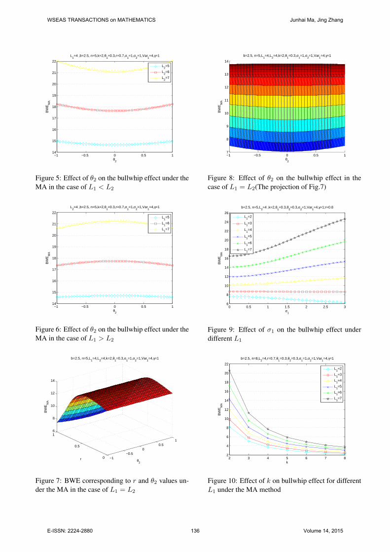


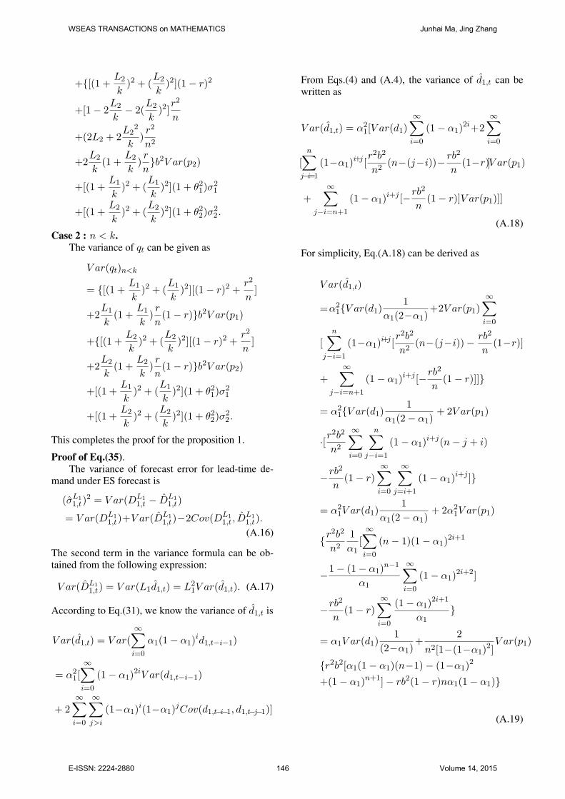


![The impact of stochastic lead times on the bullwhip effect1411.4289v3 [stat.AP] 20 Mar 2015 The impact of stochastic lead times on the bullwhip effect Zbigniew Michna∗1, Peter](https://static.documents.pub/doc/80x56/5b35355a7f8b9a330e8cf5be/the-impact-of-stochastic-lead-times-on-the-bullwhip-eect-14114289v3-statap.jpg)


