UNIVERSIT ¨ AT P OTSDAM LEHRSTUHL F ¨ UR WAHRSCHEINLICHKEITSTHEORIE UNIVERSIT ` A DEGLI S TUDI DI PADOVA DIPARTIMENTO DI MATEMATICA B ERLIN MATHEMATICAL S CHOOL Reciprocal classes of continuous time Markov Chains DISSERTATION EINGEREICHT VON GIOVANNI CONFORTI ZUR ERLANGUNG DES AKADEMISCHEN GRADES ” DOCTOR RERUM NATURALIUM” (DR. RER. NAT.) IN DER WISSENSCHAFTSDISZIPLIN S TOCHASTIK Candidate: Giovanni C ONFORTI Advisors: Prof. Dr. Paolo DAI P RA Prof. Dr. Sylvie R OELLY
UNIVERSITA DEGLI STUDI DI PADOVADIPARTIMENTO DI MATEMATICA
BERLIN MATHEMATICAL SCHOOL
Reciprocal classes of continuoustime Markov Chains
DISSERTATION EINGEREICHT VONGIOVANNI CONFORTI
ZUR ERLANGUNG DES AKADEMISCHEN GRADES”DOCTOR RERUM NATURALIUM”
(DR. RER. NAT.)IN DER WISSENSCHAFTSDISZIPLIN STOCHASTIK
Candidate:Giovanni CONFORTI
Advisors:Prof. Dr. Paolo DAI PRA
Prof. Dr. Sylvie ROELLY
This work is licensed under a Creative Commons License: Attribution 4.0 International To view a copy of this license visit http://creativecommons.org/licenses/by/4.0/ Published online at the Institutional Repository of the University of Potsdam: URN urn:nbn:de:kobv:517-opus4-82255 http://nbn-resolving.de/urn:nbn:de:kobv:517-opus4-82255
i
Summary
In this thesis we study reciprocal classes of Markov chains. Given a continu-ous time Markov chain on a countable state space, acting as reference dy-namics, the associated reciprocal class is the set of all probability measureson path space that can be written as a mixture of its bridges. These pro-cesses possess a conditional independence property that generalizes theMarkov property, and evolved from an idea of Schrodinger, who wantedto obtain a probabilistic interpretation of quantum mechanics.
Associated to a reciprocal class is a set of reciprocal characteristics, whichare space-time functions that determine the reciprocal class. We computeexplicitly these characteristics, and divide them into two main families:arc characteristics and cycle characteristics. As a byproduct, we obtain anexplicit criterion to check when two different Markov chains share theirbridges.
Starting from the characteristics we offer two different descriptions ofthe reciprocal class, including its non-Markov probabilities.The first one is based on a pathwise approach and the second one on shorttime asymptotic. With the first approach one produces a family of func-tional equations whose only solutions are precisely the elements of thereciprocal class. These equations are integration by parts on path space as-sociated with derivative operators which perturb the paths by mean of theaddition of random loops. Several geometrical tools are employed to con-struct such formulas. The problem of obtaining sharp characterizations isalso considered, showing some interesting connections with discrete ge-ometry. Examples of such formulas are given in the framework of count-ing processes and random walks on Abelian groups, where the set of loopshas a group structure.In addition to this global description, we propose a second approach bylooking at the short time behavior of a reciprocal process. In the same wayas the Markov property and short time expansions of transition probabili-ties characterize Markov chains, we show that a reciprocal class is charac-terized by imposing the reciprocal property and two families of short timeexpansions for the bridges. Such local approach is suitable to study recip-rocal processes on general countable graphs. As application of our charac-terization, we considered several interesting graphs, such as lattices, pla-nar graphs, the complete graph, and the hypercube.Finally, we obtain some first results about concentration of measure im-plied by lower bounds on the reciprocal characteristics.
ii
Zusammenfassung
Diese Dissertation behandelt die reziproke zufallige Prozesse mit Sprungen.Gegeben eine zeitkontinuierliche Markovkette als Referenzdynamik, istdie assoziierte reziproke Klasse die Menge aller Wahrscheinlichkeiten aufdem Pfadraum, die als eine Mischung ihrer Brucken geschrieben wer-den kann. Reziproke Prozesse zeichnen sich durch eine Form der bed-ingten Unabhangigkeit aus, die die Markoveigenschaft verallgemeinert.Ursprunglich ist diese Idee auf Schrodinger zuruckzufuhren, der nacheiner probabilistischen Interpretation fur die Quantenmechanik suchte.Einer reziproken Klasse wird eine Familie reziproker Charakteristiken as-soziiert. Dies sind Raum-Zeit Abbildungen, die die reziproke Klasse ein-deutig definieren. Wir berechnen diese Charakteristiken explizit und un-terteilen sie in zwei Typen: Bogen-Charakteristiken und Kreis-Charakteris-
tiken. Zusatzlich erhalten wir ein klares Kriterium zur Prufung wann dieBrucken von zwei verschiedenen Markovketten ubereinstimmen.Wir beschreiben auf zwei verschiedene Arten reziproken Klasse und beruck-sichtigen auch ihre nicht-Markov Elemente. Die erste Charakterisierungbasiert auf einem pfadweisen Ansatz, wahrend die zweite kurzzeit Asymp-totik benutzt. Der erste Ansatz liefert eine Familie funktionaler Gleichun-gen deren einzige Losungen die Elemente der reziproken Klasse sind. DieGleichungen konnen als partielle Integration auf dem Pfadraum mit einemAbleitungsoperator, der eine Storung der Pfade durch zusatzliche zufalligeKreise hervorruft, interpretiert werden. Die Konstruktion dieser Gleichun-gen benotigt eine geometrische Analyse des Problems. Wir behandelnaußerdem die Fragestellung einer scharfen Charakterisierung und zeigeninteressante Verbindungen zur diskreten Geometrie. Beispiele, fur die wireine solche Formel finden konnten, sind fur Zahlprozesse und fur Irrfahrteauf abelschen Gruppen, in denen die Menge der Kreise eine Gruppen-struktur erweist.Zusatzlich zu diesem globalen Zugang, erforschen wir eine lokale Beschrei-bung durch die Analyse des kurzfristigen Verhaltens eines reziprokenProzesses. Analog zur Markoveigenschaft und kurzzeit Entwicklung ihrerUbergangswahrscheinlichkeit Markovketten charakterisieren, zeigen wir,dass eine reziproke Klasse charakterisiert werden kann indem wir ihrereziproke Eigenschaft und zwei Familien von Kurzzeit Entwicklungen derBrucken voraussetzen. Solche lokalen Ansatz ist geeignet , um Sprung-prozesse auf allgemeine zahlbaren Graphen zu studieren. Als Beispieleunserer Charakterisierung, betrachten wir Gitter, planare Graphen, kom-plette Graphen und die Hyperwurfel.
iii
Zusatzlich prasentieren wir erste Ergebnisse uber Maßenkonzentration einesreziproken Prozesses, als Konsequenz unterer Schranken seiner Charak-teristiken.
iv
Riassunto
In questa tesi si studiano le classi reciproche delle catene di Markov.Data una catena di Markov a tempo continuo su uno spazio numerabile,che svolge il ruolo di dinamica di riferimento, la sua classe reciproca ecostituita da tutte le leggi sullo spazio dei cammini che si possono scri-vere come un miscuglio dei ponti della legge di riferimento. Questi pro-cessi stocastici godono di una proprieta di independenza condizionaleche generalizza la proprieta di Markov ed e ispirata ad un’idea avuta daSchrodinger nel tentativo di derivare un’interpretazione stocastica dellameccanica quantistica.
A ciascuna classe reciproca e associato un insieme di caratteristiche re-ciproche. Una caratteristica reciproca e una proprieta della dinamica diriferimento che viene trasmessa a tutti gli elementi della classe, e vieneespressa matematicamente da un opportuna combinazione di funzionalidel generatore della catena di riferimento. Nella tesi, le caratteristichevengono calcolate esplicitamente e suddivise in due famiglie principali:le caratteristiche di arco e le caratteristice di ciclo. Come sottoprodotto, ot-teniamo un criterio esplicito per decidere quando due catene di Markovhanno gli stessi ponti.A partire dalle caratteristiche reciproche, vengono proposte due caratter-izzazioni della classe reciproca, compresi i suoi elementi non Markoviani.La prima e basata su un approccio traiettoriale, mentre la seconda si basasul comportamento asintotico locale dei processi reciproci. Utilizzandoil primo approccio, si ottiene una famiglia di equazioni funzionali cheammette come soluzioni tutti e soli gli elementi della classe reciproca.Queste equazioni sono integrazioni per parti sullo spazio dei camminiassociate ad operatori differenziali che perturbano le traiettorie del pro-cesso canonico con l’aggiunta di loops casuali. Nella costruzione di questeequazioni si impiegano tecniche di geometria discreta, stabilendo un in-teressante collegamento con risultati recenti in questo campo. Le caratter-izzazioni ottenute sono ottimali, in quanto impiegano un numero minimodi equazioni per descrivere la classe. Con questo metodo vengono studi-ate le classi reciproche di processi di conteggio, di camminate aleatorie sugruppi Abeliani, dove l’insieme dei cicli gode anch’esso di una struttura digruppo. Il secondo approccio, di natura locale, si basa su stime asintotichein tempo corto. E ben noto come una catena di Markov sia caratteriz-zata dal fatto di possedere la proprieta di Markov e dal comportamentoin tempo corto delle probabilita di transizione. In questa tesi mostriamoche una classe reciproca e caratterizzata dalla proprieta reciproca, e da duefamiglie di stime asintotiche per i ponti del processo. Questo approccio lo-
v
cale permette di analizzare le classi reciproche di passeggiate aleatorie sugrafi generali. Come applicazione dei risultati teorici, consideriamo i lat-tici, i grafi planari, il grafo completo, e l’ipercubo discreto.Infine, otteniamo delle stime di concentrazione della misura e sul com-portamento globale dei ponti, sotto l’ipotesi di un limite inferiore per lecaratteristiche reciproche.
vi
Acknowledgments
My first thanks are for my parents. For my father, who silently inspiredme his passion for mathematics. For my mother, for having always sup-ported me with many loud words.
I thank my brother Zeno for all the interesting non-mathematical activ-ities we did together.
I owe my gratitude and my scientific growth to my advisors: Prof.SylvieRoelly taught me how to merge in a unique effort the interest for science,and the interest for persons, simply as they are. Her endless energy indealing with any aspect of the scientific life probably comes out of all thegood she sees in this. I will try to make this attitude mine.
Prof.Paolo Dai Pra introduced me to Probability some years ago, andhas never lost interest in my progresses. Besides having read all my hor-rible drafts, he knows and understands my scientific interests and prefer-ences more than anybody else, and always helped me in finding the waytowards what I like.
Even though he was not my advisor, Prof.Christian Leonard gave mea personal guided tour of Probability theory, as he likes it. This was great.
I had the pleasure to share an office and many coffees in Potsdam withSara. In Berlin I stayed with Adrian, Alberto, and Atul. I had great foot-ball conversations with Adrian, while Atul offered me lessons of RoughPath theory, and often Kebab. With Alberto we investigated in depth hischaracter of “artista maledetto”, without taking this matter too seriously.It was so much fun.
I thank Giuseppe and Matti. They have been just in front of my doorfor the past two years, always with lots of “grinta” to share with me.
I thank Paolo and Michele for all the serious and all the stupid discus-sions we had in these years over Skype and in our meetings in Paris.
I thank Niccolo, Federico e Igor. They have always been waiting forme in Verona. I will now be able to organize few of the many ”grigliate”which I have been announcing for years.
vii
Many thanks to my cousins and family. I am looking forward for stay-ing with you in San Zeno.
Anna arrived in my life right before I would leave for Berlin. How-ever, I had the easiest long-distance relationship one could imagine, sim-ply because she was so unconditionally supportive. If anything beautifulis hidden behind the calculations and proofs of this thesis, I dedicate it toher.
viii
Contents
Introduction 1
1 The Schrodinger Problem 171.1 Statement of the problem . . . . . . . . . . . . . . . . . . . . . 17
1.1.1 A small thought experiment . . . . . . . . . . . . . . . 171.1.2 Statement of the entropy minimization problem . . . 18
1.2 Representation of the solution . . . . . . . . . . . . . . . . . 191.2.1 Decomposition of the entropy . . . . . . . . . . . . . . 191.2.2 A generalized Schrodinger problem . . . . . . . . . . 23
5.5.1 The group is infinite . . . . . . . . . . . . . . . . . . . 1275.5.2 G is the cyclic group Z/NZ . . . . . . . . . . . . . . . 1295.5.3 The state space is a product group . . . . . . . . . . . 131
6 Random walks on a general graph 1336.1 Preliminaries . . . . . . . . . . . . . . . . . . . . . . . . . . . . 135
6.1.1 Directed subgraphs associated with an intensity . . . 1356.1.2 Directed subgraphs associated with a random walk . 1366.1.3 Gradients and generating sets of cycles . . . . . . . . 137
P (·|G) Conditional expectation given the σ algebra G
P (F ) Expectation of the functional F under P , sometimes also denotedEP (F )
P x A random walk started in x
P xy The xy bridge of P
P0 The initial distribution
Pt The marginal at time t ∈ [0, 1].
P01 The endpoint marginal
xiii
xiv CONTENTS
PI The image measure of XI under P
R The reference walk
XI The collection of random variables (Xt)t∈I , for I ⊆ [0, 1]
Chapter 3
Ξj The reciprocal characteristic
P The standard Poisson process
Gj The density of the reference walk w.r.t. to the Poisson process
Du Derivative operator
Chapter 4
Ξj(l, s, t) Arc characteristic
kerZ(A) The latticez ∈ ZA : Az = 0
A The set of possible jumps
A The jump matrix
pλ A multidimensional Poisson law
Φcj Cycle characteristic
θv Shift transformation in ZA
Chapter 5
(G,+) A countable Abelian group
Γ The space [0, 1]×G
SΓ The space of point measures over Γ
L + The loop-skeletons
Φνϕ∗ Reciprocal characteristics
Chapter 6
A→(k) Active arcs of the intensity k when A↔(t, k) does not depend on t
A→(P ) Active arcs of P
CONTENTS xv
A→(t, k) Active arcs of the intensity k at time t
AR→(x,Y) Set of arcs that supported by a bridge Rxy, where y ∈ Y
A↔(t, k) Symmetric extension of A→(t, k)
χa[P ](t, z → z′) Arc characteristic
χc[P ](t, c) Cycle characteristic
X (P ) Vertices visited by P
XR(x,Y) Set of endpoints of the arcs in AR→(x,Y)
xvi CONTENTS
Introduction
Reciprocal probabilities evolved from an idea of Schrodinger, who wantedto derive a stochastic interpretation of quantum mechanics.
In two papers [73] and [74] entitled “Uber die Umkehrung der Naturge-setze” and “La theorie relativiste de l’electron et l’interpretation de la mecaniquequantique” he introduced what is nowadays known as the Schrodinger prob-lem. He himself provides a neat statement of it. The following is takenfrom [74]:
Imaginez que vous observez un systeme de particules en diffusion, qui soient enequilibre thermodynamique. Admettons qu’ a un instant donne t0 vous les ayeztrouvees en repartition a peu pres uniforme et qu’a t1 > t0 vous ayez trouve un
ecart spontane et considerable par rapport a cette uniformite. On vousdemande de quelle maniere cet ecart s’est produit. Quelle en est la maniere la
plus probable ?
In mathematical terms the problem is formulated as a constrained entropyminimization problem. The entropy is taken with respect to a path mea-sure which models the motion in equilibrium of the particles, and is calledthe reference measure. The constraint is that the marginal distributions attimes t0 and t1 are prescribed by empirical observations, and it shapeswhat Schrodinger calls un ecart considerable. One year after Schrodinger,Bernstein made the observation that the Markov property may be replacedby another dependence structure, in order to better describe the dynami-cal properties of the solutions of the Schrodinger problem. His idea wasthat a more time-symmetric notion should come into play. He writes in [3]that:
“[...] si l’on veut reconstituer cette symmetrie entre le passe et le futur [...] il fautrenoncer a l’ emploi des chaınes de type Markov et les remplacer par de schemas
d’une nature differente. ”
He then introduced in [3] the reciprocal property, as a weaker version ofthe Markov property. It is a time Markov field property. At this point, it
1
2 CONTENTS
should be said that Bernstein was very likely not aware that the solutionsto the classical Schrodinger problem are indeed Markovian probabilities.Therefore it was probably not necessary to generalize the Markov propertyat that point. But the property he introduced is shaped to describe thedynamics of the solutions of a slightly modified version of the Schrodingerproblem, which we discuss in some detail in Chapter 1, and leaded tomany further fruitful mathematical developments.
The one which is of primary interest for this thesis is the study of re-ciprocal classes of Markov processes.
A mathematical rigorous study of reciprocal probabilities was initiatedby Jamison in the articles [38],[39], and [40]. He noticed that the recip-rocal property is strictly weaker than the Markov one. This observationleaded him to introduce reciprocal transition probabilities and to formu-late a list of axioms that encode the reciprocal property: they are essen-tially the reciprocal analogous of the Chapman-Kolmogorov consistencyequation. One of his results is that, given a reciprocal transition kernelsatisfying these axioms, there exists a unique reciprocal process associatedwith it.
Furthermore, Jamison explicitly characterized the covariance structureof reciprocal Gaussian processes through some differential equation. Thetheory of reciprocal Gaussian processes was further developed by Chay[12], Carmichael, Mass and Theodorescu in [11], and extended to the mul-tivariate case by Levy [50].
The concept of reciprocal class is a bit more recent, even though it ap-pears in an implicit form in [39]: it is the set of all path measures shar-ing the bridges with a given reference probability, which is assumed to beMarkovian. Many authors focused on the case when the reference prob-ability is a Brownian diffusion process: Krener started the search for re-ciprocal characteristics (often called reciprocal invariants) in [41]. He con-jectured, using short time expansion of conditional probabilities, that thereciprocal class of a Brownian diffusion is described by some special func-tionals of the drift of the reference process. Clark gave a positive answerto this question in [17, Thm 1]. He provided what he calls a “local” char-acterization of reciprocal diffusions. His result is a characterization of thereciprocal class which tells what form the semimartingale characteristics of areciprocal process should take in order for it to be in the reciprocal class ofa Brownian diffusion. Such requirements are expressed in a list of equa-tions, and each equation defines one of the reciprocal characteristics. Inthe paper [42, Thm2.1], Krener gave a full probabilistic interpretation ofthe characteristics. Each reciprocal diffusion in a reciprocal class is shownto satisfy a family of short time expansions, using heat kernel asymp-
CONTENTS 3
totics, where the coefficients of the leading terms are expressed throughthe characteristics. All these expansions are inspired by the goal of de-veloping a ’second order differential calculus’ for diffusion processes. Inparticular, the conditional mean acceleration of a Brownian diffusion con-tains all information about the reciprocal class(see equation 2.18 in [42]).In the same article, he also established that the most likely path (i.e. theminimizer of the Onsager Machlup functional) of a Brownian diffusion sat-isfies an ODE expressed in terms of the reciprocal characteristics. Someyears later, Roelly and Thieullen succeded in characterizing the whole re-ciprocal class of a Brownian diffusion in [67] and [68] including the nonMarkovian elements, using duality formulae related to Malliavin calcu-lus. Both results are condensed in the short survey [66]. This approach isbased on earlier work of Roelly and Zessin [69] who characterized the lawBrownian diffusion through a duality formula, which relates the Malli-avin derivative operator with a compensated stochastic integral operator.In contrast with Clark’s characterization, this is a non-local characteriza-tion. The derivatives which are computed there are not in short time, butare Frechet derivatives on path space. Therefore, it is a pathwise approach.The key idea Roelly and Thieullen had was to look for probabilities satis-fying the duality only within a well chosen set of directions of differenti-ation, namely the loops. Indeed, imposing the duality with respect to alldirections of differentiation is too restrictive, since the reference diffusionis then the only solution, up to its initial distribution. What we have de-scribed so far are the main mathematical steps that motivated the workof this thesis. They constitute the starting point of our investigations, to-gether with Murr’s phd thesis [56], who started to study reciprocal count-ing processes. However, many other fields of research have established afruitful interaction with the theory of reciprocal processes. Let us give avery concise overview of what seem to be the most important ones.
Stochastic Mechanics The time symmetric features of the reciprocal prop-erty inspired many authors, who continued Schrodinger’s original pro-gram in several different directions. Stochastic mechanics, which is roughlythe program of explaining quantum mechanics by using the idea that par-ticle trajectories are governed by diffusion processes, has a long history,dating back at least to Nelson’s book [58]. However, Nelson’s notion ofstochastic acceleration of a diffusion as well as Cruzeiro-Zambrini one([81, 24] in the context of Euclidean quantum mechanics) are not ”recip-rocal invariants”. It is the theory developed by Krener and Thieullen (see[41, 51, 77, 52]) that connects reciprocal processes and stochastic mechan-
4 CONTENTS
ics. Krener introduced a notion of acceleration for a diffusion process,which is different from Nelson’s acceleration and is expressed in terms ofthe reciprocal characteristics. Such an acceleration is one of the postulateswhich define the notion of solution to a “ second order” stochastic differ-ential equation : indeed the development of a second order calculus (see[77, sec.4,5] and [42, sec3]), based on reciprocal characteristics, is one ofthe most relevant contributions of these studies: to each reciprocal classis shown to be associated an Euler-Lagrange equation [77, sec 6], and afamily of conservation laws for the mass and the momentum [42, sec 5].Finally let us mention that similar ideas stand behind the Stochastic Cal-culus of variations [78], where a stochastic version of Noether’s Theoremis derived, and in [64].
Optimal transport Mikami established in [55] an interesting connectionbetween the Schrodinger problem and the Monge-Kantorovich problem.He showed that one can construct a solution to the Monge-Kantorovichproblem with quadratic cost by considering the zero-noise limit of a se-quence of static Schrodinger problems, where the reference dynamics isa Brownian motion. Leonard in [46] extended this result to arbitrary costfunctions, showing that the Monge-Kantorovich problem associated witha given cost function c is the Γ-limit of a sequence of Schrodinger problemswhere the reference dynamics obeys a Large Deviation Principle with ratefunction given by c. The fact that, in the small noise regimes, the trajec-tories of a diffusion process stay close to geodesics with very high proba-bility suggest that the limit of solutions to the Schrodinger problem con-verges to the so called displacement interpolation in optimal transport, andthis is indeed proven in [46]. This justifies the fact that sometimes solu-tions to the Schrodinger problem are called entropic interpolations.
There has been a very recent upsurge in the research around this con-nection, mostly motivated by application in control engineering, due toChen, Pavon and Georgiu. In a series of papers, they look for imple-mentable solution of the Schrodinger problem. They extended the Benamou-Brenier fluid dynamical formulation of the optimal transport problem ([16],[14] )to the Schrodinger problem, and perform explicit computations in theGaussian cases, including some degenerate situations when the diffusionmatrix of the reference process is singular.
Stochastic control Building on earlier works of Wakolbinger [79], andDai Pra and Pavon [27], Dai Pra formulated in [25] the Schrodinger prob-lem as a stochastic control problem. The control is represented by a cor-
CONTENTS 5
rection term that can be added to the drift of the reference process, and itis said to be admissible if it steers the diffusion to the desired final law attime 1. The problem is to find the control such that the resulting diffusionminimizes the relative entropy with respect to the reference diffusion. It istackled with PDE methods: the optimal control is shown to satisfy a sec-ond order Hamilton-Jacobi-Bellmann-type equation. Renewed interest inthe direction of applications stems from [15], [14].
The contribution of this thesis
This thesis contains a systematic study of reciprocal classes of continu-ous time Markov random walks on countable state spaces. We give herean overview of the results. To fix ideas, we give some definitions, whichare maybe not entirely precise at this stage, but immediate to understand.Precise statements are given in the main body of the thesis, which is inde-pendent from this short overview.
We consider a countable directed graph (X ,→). An arc from z to z′
is denoted z → z′. The whole arc set is denoted A. The space of cadlagpiecewise constant functions on X , whose jumps take place using only thearcs in A is our path space, and we call it Ω. Probabilities on Ω are calledwalks, even when they are not Markovian. A continuous time Markovwalk R on (X ,→) is specified uniquely through an intensity of jump j :[0, 1] × A → R+ and an initial distribution µ. This process is the referencewalk. The xy bridge of R is denoted Rxy and the joint law at times 0 and1 by R01. We study its reciprocal class R(R), that is, the set of randombridges of R.
R(R) :=
P =
∫supp(R01)
Rxy(·)π(dxdy);π ∈ P(X 2)
where P(X 2) is the space of probability measures on X 2
Reciprocal characteristics As we will see, a reciprocal class is constitutedby many Markov elements, such as R, all its bridges and all its Doob h-transforms, but the most of the class is made of non-Markov probabilities.The first step for understanding it is to give a criterion to decide when dotwo Markov process belong to the same reciprocal class.
Roughly all Markovian walks can be characterized via their jump in-tensity. That is, to each P ∈ P(Ω) is associated a function k(t, z → z′), such
6 CONTENTS
thatP (Xt + h = y|X[0,t]) ≈ h k(t, z → z′), as h ↓ 0
The above mentioned criterion, should be given in terms of the inten-sities. We call the set of regular intensities K :
K := k : [0, 1]×A → R+, k(·, z → z′) ∈ C1b ([0, 1]) ∀z → z′ ∈ A
It is natural to give the following informal definition:
Definition (Reciprocal characteristics). A functional χ : K → R is a re-ciprocal characteristic if and only if for any pair of Markov walks R and P ofintensities j and k respectively:
P ∈ R(R)⇒ χ(j) = χ(k) (1)
It is one of the contribution of this thesis to show existence of the char-acteristics and to compute them explicitly where the reference walk R isa random walk on a countable graph. We refer to Definition 3.2.1, Defi-nition 4.2.2, Definition 4.3.1, Corollary 5.3.1, and Definition 6.2.1, which isthe most general form. Definition 3.2.1 had already been given by R.Murrin [56].
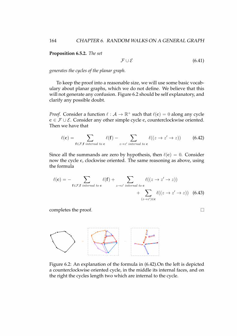
The characteristics are divided into two main categories: the arc char-acteristics and the cycle characteristics, see the two figures below.
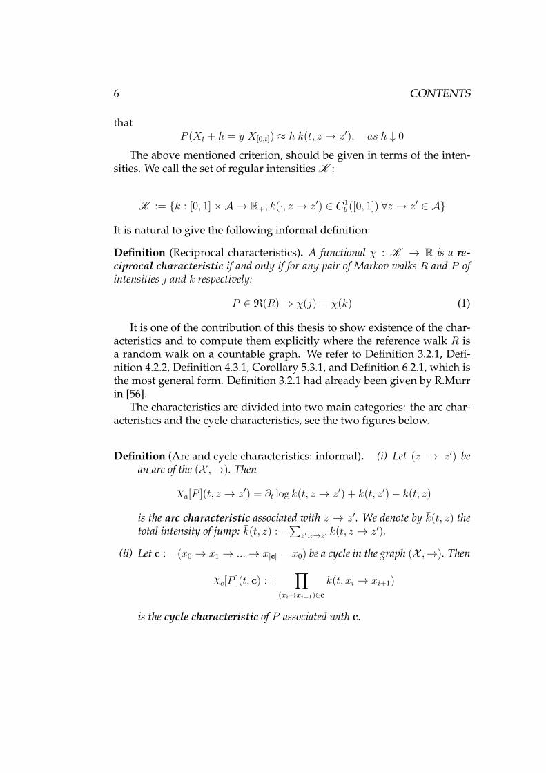
Definition (Arc and cycle characteristics: informal). (i) Let (z → z′) bean arc of the (X ,→). Then
χa[P ](t, z → z′) = ∂t log k(t, z → z′) + k(t, z′)− k(t, z)
is the arc characteristic associated with z → z′. We denote by k(t, z) thetotal intensity of jump: k(t, z) :=
∑z′:z→z′ k(t, z → z′).
(ii) Let c := (x0 → x1 → ...→ x|c| = x0) be a cycle in the graph (X ,→). Then
χc[P ](t, c) :=∏
(xi→xi+1)∈c
k(t, xi → xi+1)
is the cycle characteristic of P associated with c.
CONTENTS 7
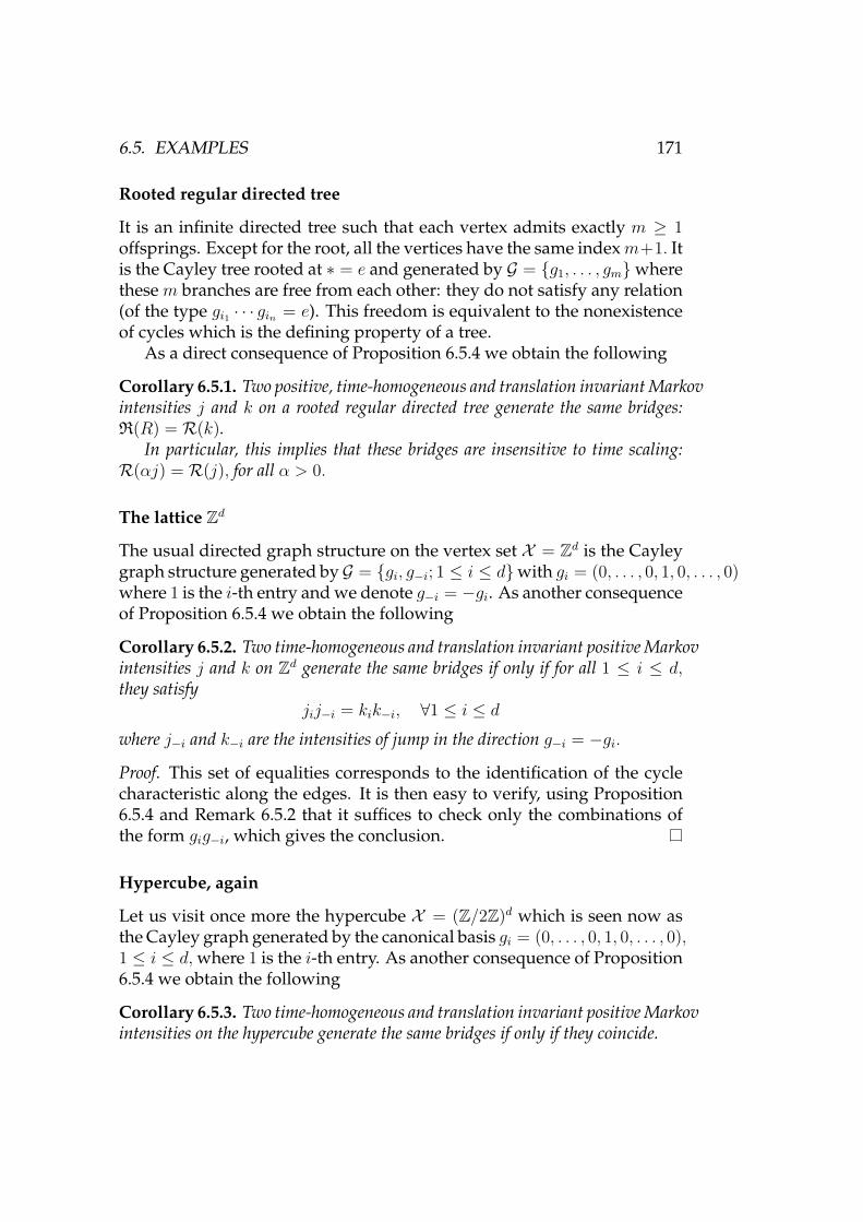
x0 x1 x3
x2
j(x1 → x2)
j(x0 → x1)
j(x2 → x0)
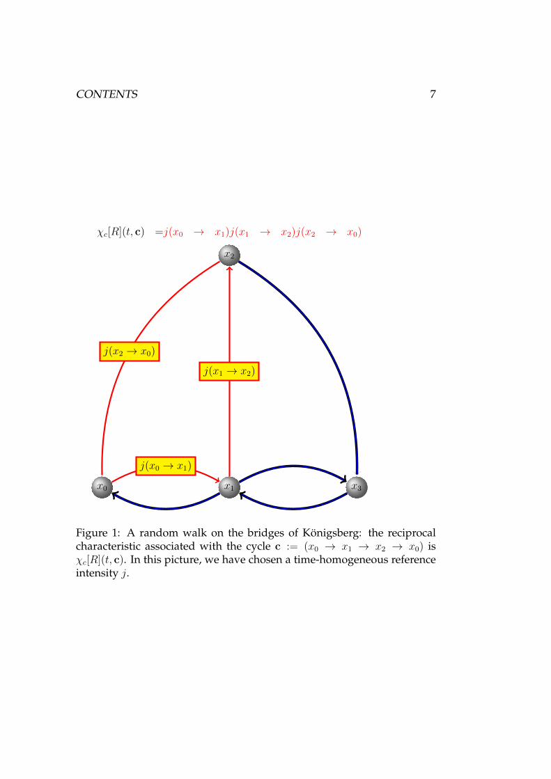
χc[R](t, c) =j(x0 → x1)j(x1 → x2)j(x2 → x0)
Figure 1: A random walk on the bridges of Konigsberg: the reciprocalcharacteristic associated with the cycle c := (x0 → x1 → x2 → x0) isχc[R](t, c). In this picture, we have chosen a time-homogeneous referenceintensity j.
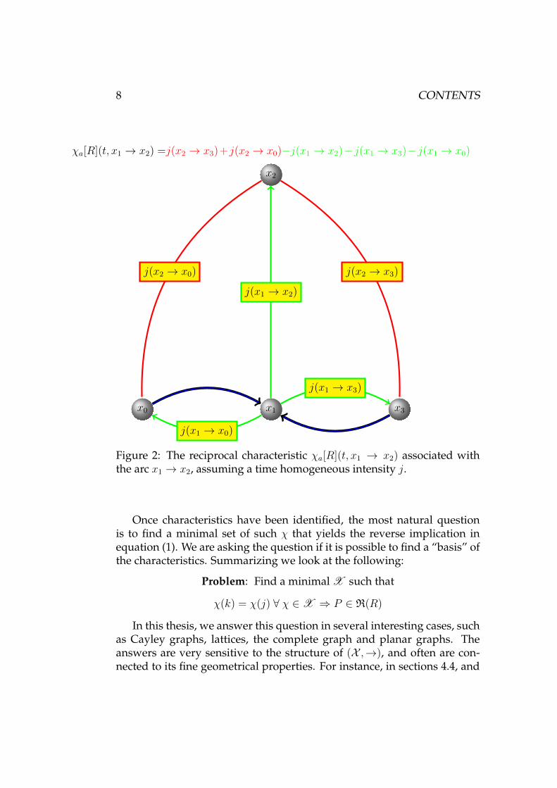
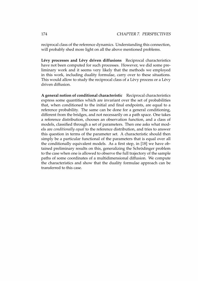
Figure 2: The reciprocal characteristic χa[R](t, x1 → x2) associated withthe arc x1 → x2, assuming a time homogeneous intensity j.
Once characteristics have been identified, the most natural questionis to find a minimal set of such χ that yields the reverse implication inequation (1). We are asking the question if it is possible to find a “basis” ofthe characteristics. Summarizing we look at the following:
Problem: Find a minimal X such that
χ(k) = χ(j) ∀ χ ∈X ⇒ P ∈ R(R)
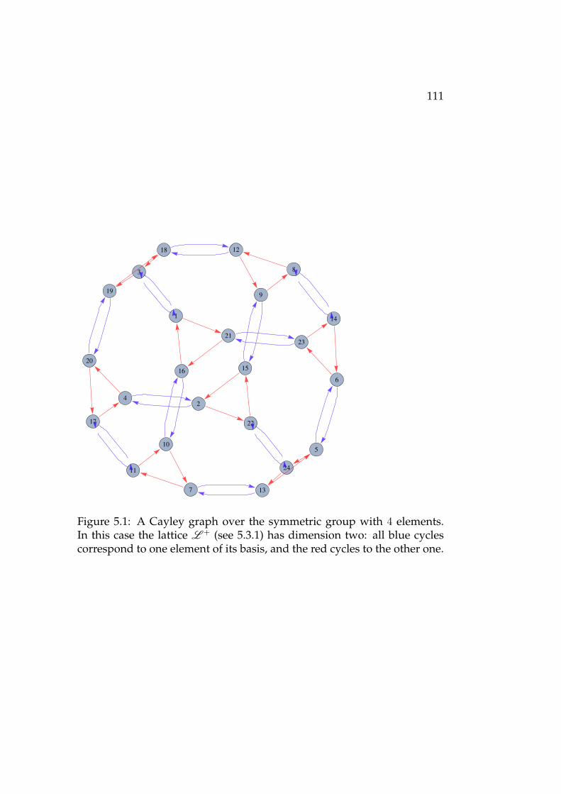
In this thesis, we answer this question in several interesting cases, suchas Cayley graphs, lattices, the complete graph and planar graphs. Theanswers are very sensitive to the structure of (X ,→), and often are con-nected to its fine geometrical properties. For instance, in sections 4.4, and
CONTENTS 9
4.5 we make use of some recent findings in discrete geometry to answerthe above-mentioned problem.
Our results contain as a byproduct an efficient criterion for checkingwhen Markov processes have the same bridges especially because it is ex-plicit in terms of the jump intensities. Other criteria have been proposed,e.g. in [32], but they are implicit and not directly checkable. On the otherhand, regarding diffusion processes, a similar result was proven by Clark[17], and in less generality by Benjamini and Lee [2].Once one has understood the full picture concerning the Markov elementsof R(R), it is the time to look at the non Markov ones. The purpose is toemploy the characteristics to go beyond the Markovian framework. Weexplored two ways of doing this: the duality formulae approach of Roellyand Thieullen [67, 68] and the short-time expansion of conditional proba-bilities.
Duality formulae: Chapters 3,4,5. With this approach one produces afamily of functional equations whose only solutions are precisely the ele-ments of R(R). One of our contributions is a fairly robust scheme to con-struct such equations, inspired by the seminal works [67, 68]. We are goingto describe it in the next lines. We use the word duality formula to equiv-alently refer to an integration by parts on path space (IBPF) or to a changeof measure formula, and we shall see IBPFs as an infinitesimal version ofchange of measure.
What we mean by change of measure formula is the following:
Definition (Change of measure formula). Let Ψ : Ω → Ω be a measurablemap. Assume that the image measure P Ψ−1 is absolutely continuous withrespect to P , and its density is GP
Ψ. Then the relation
P (F Ψ) = P (FGPΨ) ∀F ∈ B+(Ω)
is called the change of measure formula associated with Ψ.
The best known example of a change of measure formula on a pathspace is Girsanov’s Theorem. In that case Ω = C([0, 1];R), R is the Wienermeasure and for ψ regular enough, Ψ = θψ is the translation by ψ:
θψ : Ω −→ Ω, ω 7→ ω + ψ
We have that:
Gθψ := exp(∫
ψtdωt −1
2
∫ 1
0
ψ2t dt)
10 CONTENTS
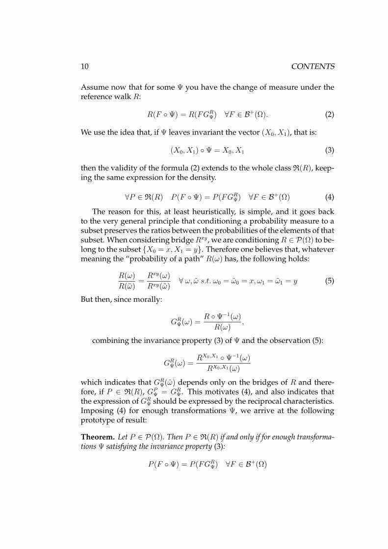
Assume now that for some Ψ you have the change of measure under thereference walk R:
R(F Ψ) = R(FGRΨ) ∀F ∈ B+(Ω). (2)
We use the idea that, if Ψ leaves invariant the vector (X0, X1), that is:
(X0, X1) Ψ = X0, X1 (3)
then the validity of the formula (2) extends to the whole class R(R), keep-ing the same expression for the density.
∀P ∈ R(R) P (F Ψ) = P (FGRΨ) ∀F ∈ B+(Ω) (4)
The reason for this, at least heuristically, is simple, and it goes backto the very general principle that conditioning a probability measure to asubset preserves the ratios between the probabilities of the elements of thatsubset. When considering bridgeRxy, we are conditioningR ∈ P(Ω) to be-long to the subset X0 = x,X1 = y. Therefore one believes that, whatevermeaning the “probability of a path” R(ω) has, the following holds:
R(ω)
R(ω)=Rxy(ω)
Rxy(ω)∀ ω, ω s.t. ω0 = ω0 = x, ω1 = ω1 = y (5)
But then, since morally:
GRΨ(ω) =
R Ψ−1(ω)
R(ω),
combining the invariance property (3) of Ψ and the observation (5):
GRΨ(ω) =
RX0,X1 Ψ−1(ω)
RX0,X1(ω)
which indicates that GRΨ(ω) depends only on the bridges of R and there-
fore, if P ∈ R(R), GPΨ = GR
Ψ. This motivates (4), and also indicates thatthe expression of GR
Ψ should be expressed by the reciprocal characteristics.Imposing (4) for enough transformations Ψ, we arrive at the followingprototype of result:
Theorem. Let P ∈ P(Ω). Then P ∈ R(R) if and only if for enough transforma-tions Ψ satisfying the invariance property (3):
P (F Ψ) = P (FGRΨ) ∀F ∈ B+(Ω)
CONTENTS 11
The construction of the Ψ, the decomposition of the density in terms ofthe reciprocal characteristics, and the fact that the formula is rich enoughto characterize R(R) are all graph-dependent problems, which have to besolved ad hoc. While it is clear how to shift paths on the Wiener space,this is far from obvious on path spaces built over graphs. Moreover, onehas to design the transformations in such a way to respect the initial andfinal state. When (X ,→) has some translation invariant structure, as itis the case for lattices or more general Cayley graphs, we found a natu-ral way of doing this, and devised the geometrical objects which allowto handle the algebraic expressions in a canonical way. We applied thisstrategy in Theorem 3.2.2, Theorem 4.3.1, and Theorem 5.3.1. In Chapter3 we look at counting processes, in Chapter 4 at lattices and in Chapter5 at Abelian groups. In going from Chapter 4 to Chapter 5, we put a ge-ometrical assumption that allows for a factorization of the cycle space ofthe graph. This assumption is crucial to obtain true pathwise formulasand is satisfied in most of the cases of interest. When this hypothesis fails,several geometrical problem arise. They are discussed in sections 4.4 and4.5. Therefore, the results of Chapter 5, which are obtained under this hy-pothesis, when applicable to the lattice case ( recall that lattices are specialinstances of Cayley graphs) not only cover the results of Chapter 4, butimprove them considerably. However, the results of Chapter 4, hold fora more general class of graphs. The resulting change of measure formu-lae are often new generalizations of other well known formulae, such asSlivnjak-Mecke identities [75, 54] or Chen’s characterization of the Poissondistribution [13].
Duality formulae correspond to a pathwise viewpoint on reciprocalprocesses, in the sense that they tell by which amount the “probabilityof a path” changes when the path is subject to a perturbation which leavesinvariant its endpoints.
In contrast with this global description, we have a corresponding lo-cal picture, which we obtain by looking at the short time behavior of areciprocal process, and is illustrated in the next paragraph.
Short time expansions: Chapter 6 This approach leads to a characteri-zation of the reciprocal class through the local (in time) behavior of its el-ements. With respect to the previous one, it has the advantage to hold forgeneral graphs, even if they do not possess any symmetry. Take a graph(X ,→). It is well known that, modulo technical conditions, the referenceMarkov random walk R is characterized by the following two properties:
12 CONTENTS
(i) The Markov property: for any s < t ∈ [0, 1], A ⊆ X :
R(Xt ∈ A|X[0,s]) = R(Xt ∈ A|Xs) R− a.s.
(ii) The jump intensity: for any z → z′ ∈ A:
R(Xt+h = z′|Xt = z) = j(t, z → z′)h+ o(h), as h ↓ 0 (6)
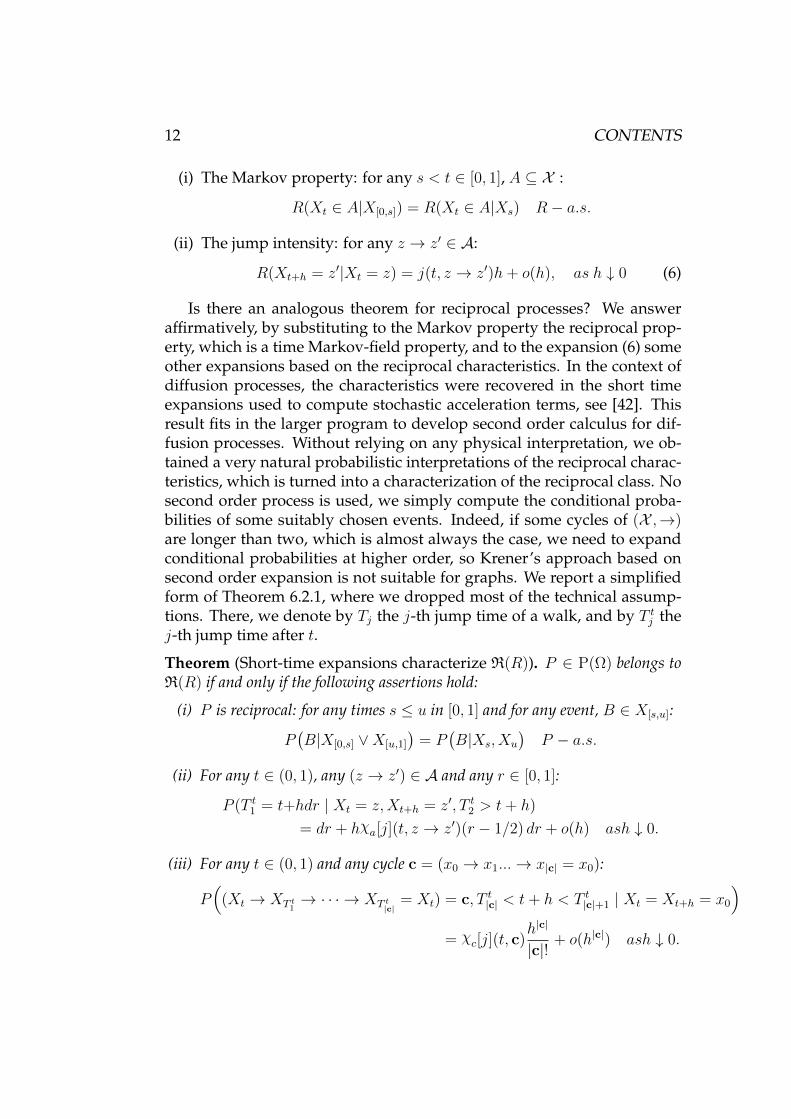
Is there an analogous theorem for reciprocal processes? We answeraffirmatively, by substituting to the Markov property the reciprocal prop-erty, which is a time Markov-field property, and to the expansion (6) someother expansions based on the reciprocal characteristics. In the context ofdiffusion processes, the characteristics were recovered in the short timeexpansions used to compute stochastic acceleration terms, see [42]. Thisresult fits in the larger program to develop second order calculus for dif-fusion processes. Without relying on any physical interpretation, we ob-tained a very natural probabilistic interpretations of the reciprocal charac-teristics, which is turned into a characterization of the reciprocal class. Nosecond order process is used, we simply compute the conditional proba-bilities of some suitably chosen events. Indeed, if some cycles of (X ,→)are longer than two, which is almost always the case, we need to expandconditional probabilities at higher order, so Krener’s approach based onsecond order expansion is not suitable for graphs. We report a simplifiedform of Theorem 6.2.1, where we dropped most of the technical assump-tions. There, we denote by Tj the j-th jump time of a walk, and by T tj thej-th jump time after t.
Theorem (Short-time expansions characterize R(R)). P ∈ P(Ω) belongs toR(R) if and only if the following assertions hold:
(i) P is reciprocal: for any times s ≤ u in [0, 1] and for any event, B ∈ X[s,u]:
P(B|X[0,s] ∨X[u,1]
)= P
(B|Xs, Xu
)P − a.s.
(ii) For any t ∈ (0, 1), any (z → z′) ∈ A and any r ∈ [0, 1]:
P (T t1 = t+hdr | Xt = z,Xt+h = z′, T t2 > t+ h)
= dr + hχa[j](t, z → z′)(r − 1/2) dr + o(h) ash ↓ 0.
(iii) For any t ∈ (0, 1) and any cycle c = (x0 → x1...→ x|c| = x0):
P(
(Xt → XT t1→ · · · → XT t|c|
= Xt) = c, T t|c| < t+ h < T t|c|+1 | Xt = Xt+h = x0
)= χc[j](t, c)
h|c|
|c|! + o(h|c|) ash ↓ 0.
CONTENTS 13
Let us comment on (ii) and (iii):
(ii) Assume that you observe a reciprocal walk of R(R) sitting in z attime t and after a short time interval you see it in z′, where z → z′ isan arc of (X ,→). Then this has essentially happened through a singlejump along z → z′. The arc characteristics χa[j](t, z → z′) accountsfor the distribution of the jump time. A positive arc characteristicimplies that this distribution is concentrated around the end of thetime interval, whereas a negative characteristic implies that the dis-tribution is concentrated around the beginning of such interval.
(iii) Assume that you observe a reciprocal walk of R(R) sitting in a statex0 at time t and you observe it there again after a short time intervalh. Given this, the probability that in the time-window [t, t + h] thewalk has traveled along the cycle c = (x0 → x1... → x|c|) is propor-tional to the reciprocal characteristic χc[j](t, c) of c and to h|c|, where|c| is the length of the cycle.
Quantitative estimates for bridges: Sections 3.3 and 4.7 A last contri-bution of this thesis is to obtain, in some special models, quantitative esti-mates on the behavior of the bridges of the reference walk. The main pointabout these results is that they hold in non-asymptotic regimes, in contrastwith the short time estimates used to characterize the reciprocal class, andthat such estimates are expressed through the reciprocal characteristics,which are the natural parameters for reciprocal classes. This is, to the bestof our knowledge, the first time when the role of reciprocal characteristicsis made explicit in global estimates concerning bridges.
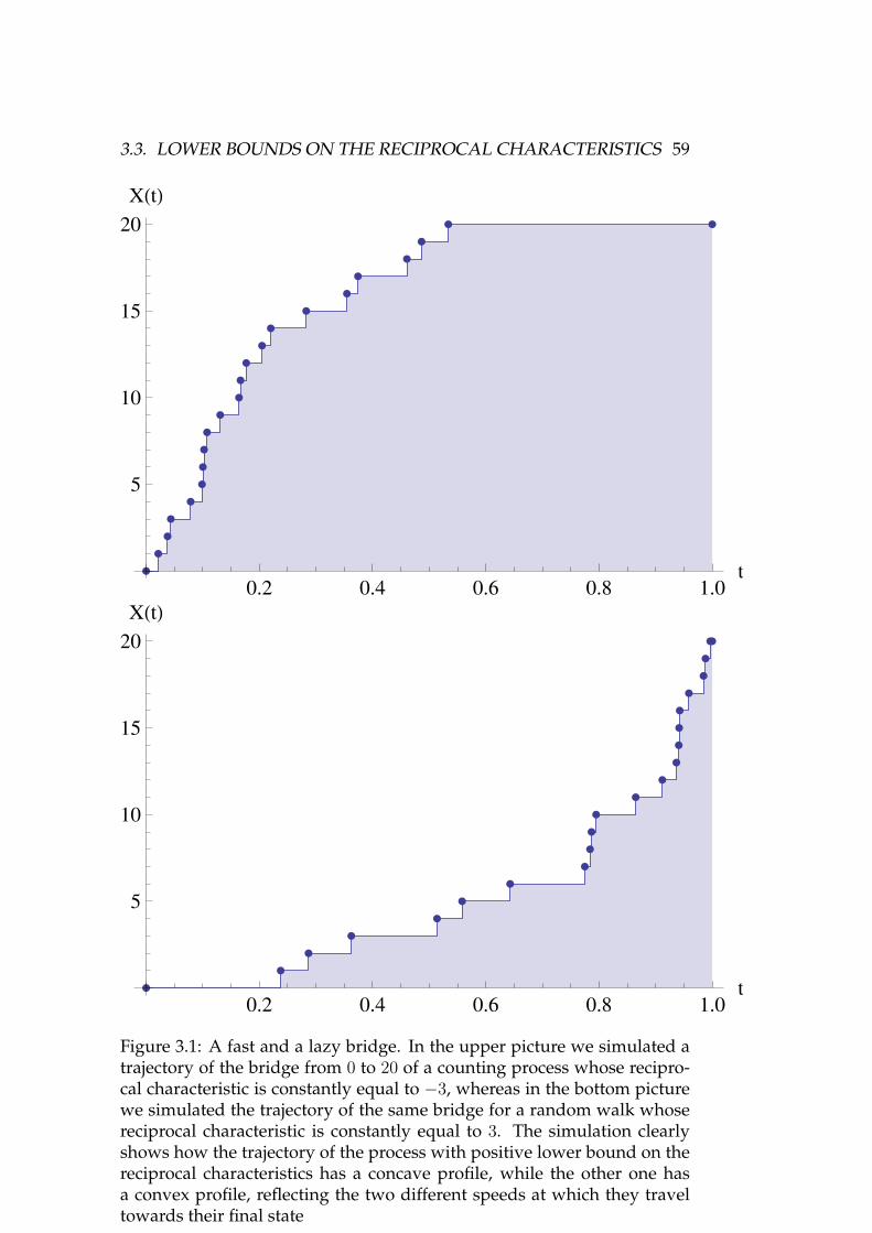
Our first result concerns counting processes, that is random walks onthe graph (Z,→), where z → z′ ⇔ z′ = z + 1. In this type of graphs,there are no cycles, and therefore only the arc characteristics matter. Alower bound one the arc characteristics Ξj is shown to imply an estimateon the last jump time of the bridges of the reference walk. In particular, apositive bound implies that the bridge of the reference walk is slower thanthe bridge of a Poisson process, in the sense that it tends to reach its finalstate later than the Poisson bridge, and we have an accumulation of thejump times around time one. The following statement formalize this. It isProposition 3.3.1.
Proposition. Let R0n be the bridge between 0 and n of R. Assume that
inft∈[0,1],0≤i≤n−1
Ξj(i, t) ≥ c ∈ R
14 CONTENTS
Then:
R0n(Tn ≤ t) ≤(
exp(ct)− 1
exp(c)− 1
)nOur second result is a concentration inequality for the number of jumps
of the bridge of a continuous time random walk on (Z,→), where theonly allowed jumps are either of size −1 or k, where k ∈ N. That is,z → z′ ⇔ z − 1z′ = z + k. Under the reference walk the number ofjumps of height k simply follows a Poisson law. This is not true underany bridge. We obtain in Chapter 4 (see Corollary 4.7.1) a characterizationof this conditional distribution with a change of measure formula, wherethe role of the cycle characteristic Φj is highlighted. What we obtain is aformula that generalizes Chen’s characterization of Poisson law, see [13].Relying on a geometrical interpolation argument (Proposition 4.7.3) andon refinements of previously established concentration of measure resultsfor the Poisson law (Proposition 4.7.1), we establish the following result.Here, by o(R) we denote a function which grows sublinearly as R→ +∞.
Theorem ( Theorem 4.7.1:informal version). Let ρ ∈ P(N) be the distributionof the number of jumps of size k under the 00 bridge of R, R00. Then there existC0 > 0 such that for all f which are 1-Lipschitz and for all R > C0:
The constant C1 does not depend on Φj . C0 might depend on it.
Let us comment very briefly on the form of the concentration rate: theleading term is governed by the geometry of the jump set, since it only de-pends on k whereas the reciprocal characteristic Φj drives the exponentialcorrection terms. Such concentration rates are not implied by any of thewell known functional inequalities, such as the family of Modified Loga-rithmic Sobolev inequality studied, among the others, in[5],[26].
The reasoning we made to obtain Theorem 4.7.1 is likely to carry overto the treatment of a more general class of models.
The concentration inequality derived here gains his interest also out-side the study of bridges of continuous time random walks. Let us clarifywhy: Chen’s characterization of Poisson random variable is the fact thatthe Poisson law of mean λ is the only law satisfying
∀f λ ρ(f(n+ 1)) = ρ(f(n)n)
The measure ρ studied in Theorem 4.7.1 is shown to be the only solutionto the change of measure formula:
∀f Φj ρ(f(n+ 1)) = ρ(f(n)γ(n))
CONTENTS 15
where γ(n) is a polynomial of degree k + 1 (recall that k is the size of thelarge jump). What is known is that to a linear coefficient on the right handside of the change of measure formula, as in Chen’s formula, correspondsa concentration inequality with rate−R logR+(log(λ)+C)R+o(R), whereC is a numerical constant. Our result shows that to a polynomial coeffi-cient on the right hand side of the change of measure formula correspondsa concentration inequality with rate−(k+1)R logR+(log(Φj)+C)R+o(R),whereC is a numerical constant. Therefore we establish a clear relation be-tween the form of the density in change of measure formulae and the rateof concentration.
16 CONTENTS
Chapter 1
The Schrodinger Problem
Outline of the chapter This short chapter is meant as an introductionto the Schrodinger problem, which shall motivate the study of reciprocalclasses. We give some heuristics that explain its formulation, and provesome structural results for its solution.
1.1 Statement of the problem
1.1.1 A small thought experiment
At time t = 0, we are given a large number Y 10 , .., Y
N0 of independent in-
distinguishable particles. As N → +∞, their empirical distribution ap-proaches a smooth profile µ0.
1
N
N∑i=1
δY i0 → µ0, as N → +∞
We let each particle travel independently from all the others with a Brow-nian motion for a unit of time. The law of large numbers tells that, asN → +∞ the empirical measure at time 1, which we call µ1, approachesµ1, defined by:
µ1(dy) :=
∫Rr(y|x)µ0(dx),
where r is the Gaussian kernel. We are allowed to observe the empiricalmeasure µ1 at time 1. Schrodinger question is the following:
Given that N is very large and µ1 is significantly different from µ1, what is themost likely behavior of the whole random system?
17
18 CHAPTER 1. THE SCHRODINGER PROBLEM
We can sketch an heuristic based on the theory of large deviationswhich explains the mathematical formulation of this question. Such ar-gument was made rigorous by Follmer in [34].
We call LN the empirical measure associated to the particle system.Note that such a measure is defined over the space Ω of continuous trajec-tories, rather than on R, as it was the case for µ0 and µ1.
LN :=1
N
N∑i=1
δ((Y it )t∈[0,1])
We denote by Prob the distribution of Ln . The law of large number tellsthat LN converges to a Brownian motion started in µ0, whose law R iscalled the reference dynamics. Our observations concerning the initial andfinal configurations of the particles tell us that:
LN ∈ P : P0 = µ0, P1 = µ1 (1.1)
Using informally Sanov’s Theorem (see [29, sec 6.2]) we have that,when N is very large the distribution of LN is governed by the relativeentropy H(·|R):
Prob(LN ∈ A) ≈ exp(−N infP∈A
H(P |R)) ∀A ⊆ P(Ω)
In this interpretation, the “most likely” evolution is clearly given by theminimizer of H(·|R) within the set of measures matching our observation,described in (1.1). We arrive at :
H(P |R)→ min P ∈ P(Ω), P0 = µ0, P1 = µ1
This is the Schrodinger problem.
1.1.2 Statement of the entropy minimization problem
In this section we state rigorously the problem we have just discussed. Al-thought in the presentation above particles were moving according to aBrownian motion, the same questions can be asked in a much more gen-eral setting, replacing the Brownian motion with another Markov process.Indeed, in this thesis, we will be concerned with random walks on graphs.We consider a Polish state space X . The cadlag space over it is denotedΩ, and the canonical process (Xt)t∈[0,1]. All the standard conventions forsigma algebras and filtrations can be read in the table of notation.
1.2. REPRESENTATION OF THE SOLUTION 19
Definition 1.1.1. The dynamic Schrodinger problem associated with R ∈ P(Ω),µ0, µ1 ∈ P(X ) is the following entropy minimization problem:
H(P |R)→ min P ∈ P(Ω), P0 = µ0, P1 = µ1 (1.2)
where µ0, µ1 ∈ P(X ) are the prescribed marginals.
Projecting this problem onto the marginals at times t = 0, 1 gives the,apparently simpler, static Schrodinger problem. For π ∈ P(X 2), i ∈ 0, 1,the image measure π (Xi)
−1 is denoted by πi.
Definition 1.1.2. The static Schrodinger problem associated withR ∈ P(Ω),µ0, µ1 ∈P(X 2) is the following entropy minimization problem:
H(π|R01)→ min P ∈ P(X 2), π0 = µ0, π1 = µ1 (1.3)
As it is clear from the formulation, there is more than an analogy withan optimal transport problem. Indeed it is shown in [55] and [46] thatthe classical Monge-Kantorovich problem can be obtained as the limit ina suitable sense of a sequence of (static) Schrodinger problems through a”slowing down” procedure.
1.2 Representation of the solution
1.2.1 Decomposition of the entropy
The first result of this subsection is that is Proposition (1.2.1), which saysthat the two problems are indeed equivalent. If one can solve the dynam-ical problem the solution to the static problem is given by a simple projec-tion. The converse is also true. Given a solution to the static problem oneobtains a solution to the dynamical problem by mixing bridges of the ref-erence measure according to the solution of the static problem. This wasfirst proven by Follmer [34], although in a less general setting.
Before presenting the result, we recall that under the current hypothe-ses, both Ω and X 2 are Polish spaces, and the projection (X0, X1) : Ω→ X 2
is measurable. Therefore there exist a regular conditional probability asso-ciated with it, that is, there exist a measurable map P xy : X 2 → P(Ω) suchthat for all A ∈ F :
P (A) =
∫X 2
P xy(A)P01(dxdy)
The P − a.s. well defined measure P xy is called the xy bridge.
20 CHAPTER 1. THE SCHRODINGER PROBLEM
Under the current assumptions for any P ∈ P(Ω), π ∈ P(X 2), π P01
the probability measure ∫X 2
P xy(·)π(dxdy)
is well defined. Having said this, we can prove the equivalence betweenthe two problems, following [49].
Proposition 1.2.1. Let µ0, µ1 ∈ P(X ) be fixed. The dynamical and static Schrodingerproblems both admit at most one solution. If P solves the dynamical problem thenπ := P01 solves the static problem associated with R. Conversely, if π solves thestatic problem, then
P =
∫X 2
Rxy(·)π(dxdy) (1.4)
solves the dynamical problem.
Proof. Since the admissible region for both problem is a convex subset ofeither P(Ω) or P(X 2) and the relative entropy is a strictly convex function,both problems admit at most one solution. Assume now that P solves(1.2). Using the well known disintegration formulas for the relative en-tropy:
H(P |R) =
∫H(P xy|Rxy)P01(dxdy) +H(P01|R01)
we deduce that P xy = Rxy P01 − a.s., for otherwise the probability
P (·) =
∫X 2
Rxy(·)P01(dxdy)
would be such that H(P |R) < H(P |R), which contradicts the optimalityof P .
Consider now any other π in the admissible region of (1.3). Then themeasure
Qπ(·) =
∫X 2
Rxy(·)π(dxdy)
is well defined.Using again the disintegration formula for the relative entropy we have
that H(Qπ|R) = H(π|R01) and H(P |R) = H(P01|R01). But since P solvesthe dynamic problem , then H(π|R01) > H(P01|R01). This proves that πsolves the static problem.
Conversely, let π a solution of the static problem and consider P asin (1.4). The disintegration formula for the relative entropy tells us that
1.2. REPRESENTATION OF THE SOLUTION 21
H(P |R) = H(π|R01). Let us remark that P is well defined under the cur-rent hypothesis. Consider now any Q in the admissible region of the dy-namical problem. Then Q01 is clearly in the admissible region of (1.3).Using the disintegration formula for the entropy we have:
H(Q|R) =
∫H(Qxy|Rxy)Q01(dxdy) +H(Q01|R01)
As the relative entropy is always non negative, and by assumptionH(Q01|R01) ≥H(π|R01) = H(P |R) , we conclude that H(Q|R) ≥ H(P |R) and the conclu-sion follows.
The following proposition gives some information on the shape of theminimizers. It tells that the density of the solution decouples in a productof two functions f(X0)g(X1).
f, g can also be found as solutions to the so called Schrodinger system,for which Fortet [35] and Beurling [4] proved the first existence results.A more general statement can be found in Section 2 of [48], where finequestions concerning the support of R01 are discussed. For the sake ofsimplicity, we present a simpler version Theorem 2.8 of [48] under theslightly more restrictive assumption as considered by Ruschendorff andThomsen [71, Thm 3].
Proposition 1.2.2. Assume that R01 R0 ⊗ R1, and that for some π in theadmissible region, H(π|R01) < +∞. Then the static problem admits a uniquesolution π and there exist two measurable functions f, g : X → R+ such that
π = f(X0)g(X1)R01 (1.5)
The functions f, g are R01 − a.s. solutions to the Schrodinger system:dµ0
dR0(x) = f(x)R(g(X1)|X0 = x)
dµ1
dR1(y) = g(y)R(f(X0)|X1 = y)
(1.6)
We do not give the proof of this theorem here, since the measure-theoreticalarguments needed to show existence part are quite technical, and not strictlyrelated to the content of this thesis. We shall rather give an intuitionon why convex optimization techniques can be used to prove the fac-torization (1.5). The same ideas provide an informal derivation of theSchrodinger system.
22 CHAPTER 1. THE SCHRODINGER PROBLEM
Consider any π in the admissible region of the static problem. Thefollowing representation of the relative entropy is well known:
H(π|R01) = sup∫X 2
udπ : u ∈ Cb(X 2),
∫X 2
exp(u)dR01 = 1
(1.7)
Consider now ϕ, ψ ∈ Cb(X ) and define ϕ⊕ ψ ∈ Cb(X 2) as follows:
ϕ⊕ ψ(x, y) := ϕ(x) + ψ(y)
Choosing u = ϕ ⊕ ψ in (1.7), and using the fact that π0 = µ0, π1 = µ1 weobtain:
H(π|R01) ≥∫Xϕdµ0 +
∫Xψdµ1, ∀ϕ, ψ s.t.
∫X 2
exp(ϕ⊕ ψ)dR01 = 1
Let us note that the right hand side of the last identity is independent fromthe choice of π. Therefore,the optimal value of∫
Xϕdµ0 +
∫Xψdµ1 → max, ϕ, ψ ∈ Cb(X ),
∫X 2
exp(ϕ⊕ ψ)dR01 (1.8)
is a lower bound for the optimal value of the Schrodinger problem. In-deed, (1.8) is the dual problem of (1.4). In [45] it is proven that the optimalvalues of the two problems in most of the cases coincide, and are both at-tained. Now, assume that we are in one of these cases. If π is the solutionto the static Schrodinger problem and ϕ, ψ is an optimal pair for the dualproblem (1.8) we have:
H(π|R01) =
∫Xϕdµ0 +
∫Xψdµ1 =
∫X 2
ϕ⊕ ψdπ
one gets that:dπ
dR01
= exp(ϕ⊕ ψ)
which partially explains (1.5), with f = exp(ϕ), g = exp(φ). Consideringthe marginals, we obtain:
dπ0
dR0(x) = f(x)R01(g(X1)|X0 = x)
dπ1
dR1(y) = g(y)R01(f(X0)|X1 = y)
But,since π is in the admissible region, π0 = µ0, π1 = µ1, and this givesthe system (1.6). For more details, we redirect the interested reader to theproof of Theorem 2.8 in [46]. An interesting consequence Theorem 1.2.2is that the solution of (1.2) inherits the Markov property from R. We onlysketch the proof, since it will follow as a special case of a more generalstatement, which we prove in Proposition 2.2.3.
1.2. REPRESENTATION OF THE SOLUTION 23
Proposition 1.2.3. Assume that R01 R0 ⊗ R1 and that R is a Markov mea-sure. Then the solution to the dynamical problem exists and it is also a Markovprobability.
Proof. Thanks to Proposition 2.2.2 the static problem admits a solution πwhich takes the form 1.5 . Applying Proposition 1.2.1 the dynamical prob-lem also admits a solution, which is:
P =
∫X 2
Rxyπ(dxdy) =
∫X 2
Rxyf(x)g(y)R01(dxdy)
which is equivalent to say that
P R, anddP
dR= f(X0)g(X1) R− a.s.
It will be proven in Proposition 2.2.3 that if R is Markov and P takes theform above, then P is Markov as well.
It is curious that, at this stage, there doesn’t seem to be any need for ageneralization of the Markov property to study the solution Schrodingerproblem. Indeed Bernstein, in his 1932 paper was not aware that solutionsof the Schrodinger problems are Markov. It seems that this has been firstbeen pointed out by Jamison in [39]. However, the reciprocal property,which Bernstein introduced in the same work, is shown to describe exactlythe dependence structure of solutions of a very natural generalization ofthe problem discussed above. That is, we impose a constraint not only onthe endpoint marginals separately, but we also prescribe their dependencestructure.
The constraint then changes from
P0 = µ0, P1 = µ1
to
P01 = µ ∈ P(X 2)
1.2.2 A generalized Schrodinger problem
We now turn the attention to the generalized Schrodinger problem:
Definition 1.2.1. We define the following entropy minimization problem, asso-ciated with R ∈ P(Ω), µ ∈ P(X 2):
H(P |R)→ min P ∈ P(Ω), P01 = µ
24 CHAPTER 1. THE SCHRODINGER PROBLEM
Let us note that there is not a static problem associated to this prob-lem, as P01 is fixed within the admissible region. As in Proposition 1.2.1we have a nice constructive result for the solution to (1.2.1): It says thatthe solution is a random bridge of R, where the mixing measure is givenprecisely by µ, rather than the solution of the static problem (1.3). We skipthe proof, as it is completely analogous to that of Proposition 1.2.1.
Proposition 1.2.4. The problem (1.2.1) admits a solution if and only ifH(µ|R01) <+∞ . In this case, the solution is:
P =
∫X 2
Rxyµ(dxdy) (1.9)
Solutions to this last problem are truly reciprocal probabilities. Thegoal of the next section is to introduce the reciprocal property and givesome very general notion about reciprocal probabilities. As a by product,we will obtain that P defined in (1.9) is indeed reciprocal.
Chapter 2
Reciprocal processes andcontinuous time Markov chains
Outline of the chapter The aim of this chapter is to lay the foundationsfor the study of reciprocal probabilities on discrete structures. We reviewsome basic general results and introduce the concept of reciprocal class of aMarkov probability. It is shown to be the set of solution to the generalizedSchrodinger problem introduced in the first chapter. We define the mainobject of study for this thesis: the reciprocal class of a Markov Chain. Asa technical tool, which will be used systematically later on, a GirsanovTheorem for continuous time Markov chains is presented at the level ofgenerality needed in this thesis.
The recent survey [49] introduces a measure-theoretical viewpoint onreciprocal processes, in contrast with Jamison reciprocal transition proba-bilities, and collects many basic results. It serves as a guideline for the firsttwo sections of this chapter.
Organization of the chapter Section 2.1 is a self-contained introductionto reciprocal probabilities. Reciprocal classes are studied in Section 2.2.A first representation results for reciprocal classes is shown at Proposi-tion 2.2.2. In Section 2.3 we specify our notations about continuous timeMarkov chains, and the assumptions on the reference measure. As a usefultool for the next chapters, a Girsanov theorem is proved.
25
26 CHAPTER 2. RECIPROCAL CLASSES
2.1 The reciprocal property
2.1.1 Definition
A simple description of the Markov property of a probability is that, giventhe current state Xu, the sigma algebras X[0,u] and X[u,1] are independent.That is, X[0,u] and X[u,1] are independent under P (·|Xu).
The reciprocal property is the fact that for any pair of times s < u, giventhe position (Xs, Xu) of the process at these two times, the behavior of theprocess in [s, u] is independent from the past up to s and the future from uon. Speaking about sigma algebras, we ask that X[s,u] is independent fromσ(X[0,s] ∨X[u,1]) given (Xs, Xu). The property we have just stated coincidewith that of a Markov field, indexed by time, and reciprocal probabilitiescan also be seen from this point of view.
Definition 2.1.1. A probability measure P on Ω is called reciprocal if for anytimes s ≤ u in [0, 1] and for any event, B ∈ X[s,u]:
P(B|X[0,s] ∨X[u,1]
)= P
(B|σ(Xs, Xu)
)P − a.s. (2.1)
Remark 2.1.1. For any sigma algebra G, P(B|G) is an equivalent notation for
the random variable P (1X∈B|G). We shall use both expressions, depending on thecontext.
From the very definition of the reciprocal property, one immediatelysees a nice time-simmetry, where future and past are somehow exchange-able: a probability is reciprocal if an only if the time-reversed probabilityis so (see Theorem 2.2 of [49]). This is also true for Markov probabilities,but maybe less transparent from the definition.
2.1.2 The relation with the Markov property
Here, we show some of the most interesting properties of reciprocal proba-bilities. We follow the guidelines of [49], which relies on Jamison’s originalpresentation.
At first, let us show that the reciprocal property is indeed a weakeningof the Markov property.
Proposition 2.1.1. Any Markov probability is reciprocal.
2.1. THE RECIPROCAL PROPERTY 27
Proof. We check directly Definition 2.1.1. The proof consists of two chainsof identities. These identities are obtained one from the other using eitherthe Markov property (in this case we mark the equality with (M)) or someof the properties of conditional expectation, ( if so, we mark the equalitywith (E)). First we show that for any A ∈ X[0,s], C ∈ X[u,1]:
P(1A 1C |Xs, Xu
)= P
(1A|Xs
)P(1C |Xu
). (2.2)
For this purpose, let us pick any pair of measurable sets D,F ⊆ X . Wehave
P (1A 1D(Xs)1F (Xu)1C))(E)= P (1A 1D(Xs)1F (Xu) P (1C |X[0,u]))
(M)= P (1A 1D(Xs)1F (Xu) P (1C |Xu))(E)= P (P (1A|X[s,1]) 1D(Xs)1F (Xu) P (1C |Xu))
(M)= P (P (1A|Xs) 1D(Xs)1F (Xu) P (1C |Xu)),
from which (2.2) follows by the very definition of conditional expecta-tion.
Consider now any triplet of events A,B,C such that A ∈ X[0,s], B ∈X[s,u], C ∈ X[u,1]. We have:
P (1A1B1C)(E)= P (1A 1B P (1C |X[0,u]))
(M)= P (1A 1B P (1C |Xu))(E)= P (P (1A|X[s,1]) 1B P (1C |Xu))
(M)= P (P (1A|Xs) 1B P (1C |Xu))(E)= P (P (1A|Xs)P (1B|Xs, Xu)P (1C |Xu))
(2.2)= P (P (1A1C |Xs, Xu)P (1B|Xs, Xu))(E)= P (1A1CP (1B|Xs, Xu)).
Since A,C were arbitrarily chosen in X[0,s], X[u,1], we have shown that
∀B ∈ X[s,u], P (1B|X[0,s], X[u,1]) = P (1B|Xs, Xu) P − a.s.
This shows that P is reciprocal.
The reciprocal property is not equivalent to the Markov property. Weconstruct here a simple counterexample, based on the Poisson process.
28 CHAPTER 2. RECIPROCAL CLASSES
Example 2.1.1. Let X = N andR be the Poisson process with initial distribution12δ0+1
2δ1, where δ denotes the Dirac measure. We consider P = 1
2R01(·)+1
2R12(·),
where R01 is the Poisson bridge from 0 to 1 and R12 is the Poisson bridge from 1to 2. It is easy to see that one has:
P (X1 = 1|X 12
= 1) =R01(X 1
2= 1)
R01(X 12
= 1) +R12(X 12
= 1)< 1
because R12(X 12
= 1) > 0.However:
P (X1 = 1|X 12
= 1, X0 = 0) = 1
This shows that P is not a Markov probability. But, thanks to Proposition2.2.2, which we will prove below, P is reciprocal. Indeed the density dP
dRis mea-
surable with respect to the initial and final state. One can check that:
dP
dR=
1
e1(0,1),(1,2)(X0, X1)
The next result is a sufficient condition for a reciprocal probability tobe Markov.
Proposition 2.1.2. Let P ∈ P(Ω) be reciprocal. If either X0 or X1 is almostsurely constant, then P has the Markov property.
Proof. Assume, w.l.o.g. that X1 is a.s. constant and take any f ∈ B(X ).Then we have that, for any s ≤ u:
P (f(Xu)|X[0,s]) = P (f(Xu)|X[0,s], X1).
Using the reciprocal property and the hypothesis:
P (f(Xu)|X[0,s], X1) = P (f(Xu)|Xs, X1) = P (f(Xu)|Xs),
which gives the conclusion.
2.2 The concept of reciprocal class
2.2.1 Probabilities with the same bridges
Given a reference Markov probabilty R, (which plays the role of the ref-erence dynamics in the Schrodinger Problem), the associated reciprocalclass is the set of all bridge mixtures of R. In this sense, it can be seen as
2.2. THE CONCEPT OF RECIPROCAL CLASS 29
the set of ”random bridges” of R. Using Proposition 1.2.1, one sees thatas the constraint π varies, the set of solutions to the modified Schrodingerproblem (1.2.1) forms a reciprocal class.
In the rest of the thesis, we make the assumption that the state spaceX is countable. When X is not countable, one has to make a distinctionbetween reciprocal family and reciprocal class because the bridges of thereference process may not be everywhere well defined, but only R-almostsurely (see Section 2 of[49]). But since X is assumed to be countable the xybridge Rxy ∈ P(Ω) is everywhere well defined on the set support or R01,and there is no need to distinguish here.
Definition 2.2.1. (Reciprocal Class) Let R be a Markov probability. We definethe following subset of probability measures:
R(R) :=
P =
∫supp(R01)
Rxy(·)π(dxdy); π ∈ P(X 2), supp(π) ⊆ supp(R01)
as the reciprocal class of R.
The next proposition is a general recipe to construct reciprocal proba-bilities as mixtures of the bridges of a reciprocal reference measure. Sinceany Markov probability is also reciprocal, as a by product we obtain thatthe elements of R(R) are indeed reciprocal probabilities in the sense ofDefinition 2.1.1.
Proposition 2.2.1. Let R be a reciprocal probability. Then, for any π ∈ P(X 2)such that suppπ ⊆ suppR01 the measure P defined by:
P (·) =
∫X 2
Rxy(·)π(dxdy) (2.3)
is a reciprocal probability. Moreover, P also satisfies
i) For all (x, y) ∈ suppP01:
P xy = Rxy P01 − a.s. (2.4)
ii) For all s ≤ u
P (·|Xs, Xu) = R(·|Xs, Xu) P − a.s. (2.5)
Proof. We check directly Definition 2.1.1. Consider s ≤ u andA ∈ X[0,s], B ∈X[s,u], C ∈ X[u,1]. In the same spirit as the proof of Proposition 2.1.1, when-ever an equality is obtained with an application of the reciprocal property
30 CHAPTER 2. RECIPROCAL CLASSES
we mark it with (R). We have:
P (1A1B1C) =
∫supp (π)
1
R01(x, y)R(1A1B1C1X0,X1=(x,y))π(dxdy)
(R)=
∫supp (π)
1
R01(x, y)R(1AR
(1B|Xs, Xt)1C1X0,X1=(x,y)
)π(dxdy)
= P (1AR(1B|Xs, Xt)1C)
By the very definition of conditional expectation, we conclude that
P (1B|X[0,s], X[u,1]) = R(1B|Xs, Xu) ∀B ∈ X[s,u].
But then:
P (1B|Xs, Xu) = P (P (1B|X[0,s], X[u,1])|Xs, Xu)
= P (R(1B|Xs, Xu)|Xs, Xu) = R(1B|Xs, Xu)
from which both the fact that P is reciprocal and ii) follow.Claim i) on the equality of the bridges follows by ii) considering s =
0, u = 1.
Using this last proposition, we can see the announced fact that solu-tions to the generalized Schrodinger problem are indeed reciprocal proba-bilities. The last proposition has the following interesting corollary:
Corollary 2.2.1. If a solution to the entropy minimization problem (1.2.1) exists,then it is a reciprocal probability.
Moreover, combinig Proposition 2.2.1 with 2.1.2 we get:
Corollary 2.2.2. Bridges of reciprocal probabilities are Markov probabilities.
2.2.2 A representation result
The next result, which will be very useful later on, says that a probabil-ity belongs to the reciprocal class if and only if its density w.r.t. to thereference measure R is of a particular form. It has to be compared withProposition 2.2.3.
Proposition 2.2.2. Let P ∈ P(Ω). Then P ∈ R(R) if and only if P R anddPdR
is (X0, X1)-measurable.
2.2. THE CONCEPT OF RECIPROCAL CLASS 31
Remark 2.2.1. If the state space is not countable, one cannot expect that membersof the reciprocal class are dominated by the reference measure, because bridges arenot.
Proof. (⇒) Let P ∈ R(R). Then, since X is countable, then for any (x, y) ∈suppR01, Rxy Rx. By mixing we obtain that P R. Let us denote itsdensity by M . We have, for all F ∈ B+(Ω), using repeteadly the propertiesof conditional expectation and the definition of R(R):
R(R(M |X0, X1)F ) = R(R(M |X0, X1)R(F |X0, X1))
= R(MR(F |X0, X1))
=︸︷︷︸P∈R(R)
R(MP (F |X0, X1))
= P (P (F |X0, X1))
= P (F )
= R(MF )
From this it follows that M = R(M |X0, X1), which gives the conclusion.(⇐) Assume that P R(R) and the density (which again we denote
by M ) is (X0, X1) measurable. Then M = R(M |X0, X1) R − a.s.. LetF ∈ B+(Ω), and Z be (X0, X1)-measurable. We have, again by the verydefinition of conditional expectation:
P (R(F |X0, X1)Z) = R(R(F |X0, X1)) MZ︸︷︷︸(X0,X1)−measurable
)
= R(F MZ)
= P (F Z)
= P (P (F |X0, X1) Z)
From which it follows that R(F |X0, X1) = P (F |X0, X1) P − a.s., andhence the conclusion.
2.2.3 Markov probabilities of a reciprocal class
By proving the next proposition we also complete the proof of Proposi-tion 1.2.3 about the Markovianity of solutions to the Schrodinger Problem.We show that transforming a reference Markov probability R with a den-sity enjoying the multiplicative decomposition (2.6) preserves Markovian-ity. Such a measure transformation generalizes the Doob h-transform [30].More precisely, it is a time symmetric version of it.
32 CHAPTER 2. RECIPROCAL CLASSES
Proposition 2.2.3. Let R be Markov and P ∈ P(Ω). Assume that there existf, g : X → R+ such that:
P = f(X0)g(X1)R R− a.s. (2.6)
Then P is also Markov.
The proof is based on the following well known lemma.
Lemma 2.2.1. Let P R and M = dPdR
. Then, for every F ∈ B+(Ω):
P (F |Xt) =R(MF |Xt)
R(M |Xt)P − a.s. (2.7)
Proof. First note that no division by zero on the right hand side occursP − a.s.. We have, with the basic properties of conditional expectation:
P (F 1A(Xt)) = R(MF 1A(Xt))
= R(R(M |Xt)
MF 1A(Xt)
R(M |Xt)
)= R
(R(M |Xt)
R(MF |Xt)1A(Xt)
R(M |Xt)
)= R
(MR(MF |Xt)1A(Xt)
R(M |Xt)
)= P
(R(MF |Xt)
R(M |Xt)1A(Xt)
)The conclusion follows by the definition of conditional expectation.
Proof. We have to show that for any A ∈ X[0,t], any B ∈ X[t,1]:
P (1A1B|Xt) = P (1A|Xt)P (1B|Xt). (2.8)
Using Lemma 1 and the Markov property of R:
P(1A1B|Xt
)=
R(f(X0)1A1Bg(X1)|Xt
)R(f(X0)g(X1)|Xt)
)=
R(f(X0)1A|Xt)
R(f(X0)|Xt)
R(1Bg(X1)|Xt)
R(g(X1)|Xt)(2.9)
Applying twice Lemma 2.2.1 and the Markov property we obtain thatP (1A|Xt)P (1B|Xt) coincides with the expression in (2.9). This concludesthe proof.
We refer to [44] for more details about the infinitesimal generator asso-ciated with P defined as in (2.6). It is expressed in terms of the solutionof the Kolmogorov backward PDE associated with the generator of R andthe “carre du champ” operator.
2.3. OUR FRAMEWORK 33
2.3 Our framework
This section is devoted to a precise definition of our main object of study:the reciprocal class R(R) of a continuous time Markov Chain R, which iscalled the reference walk. Markov chains are essentially Markov processeson countable state spaces, and are among the most studied class of pro-cesses in Probability theory. Some very general references are the books[60],[8]. In this thesis only continuous time Markov chains are considered.
Our main goals in the next chapters will be to compute the reciprocalcharacteristics associated with a reciprocal class R(R), give their probabilis-tic interpretation, and characterize R(R) by means of the characteristics.
Since the Markov chains we will consider in the next chapter are ofquite different nature, we need to establish a common framework and no-tation to treat them: this is done in 2.3.1. Even more notation on graphswill be required in Chapter 6, see section 6.1. In the first two subsections,we specify the main assumptions on the reference walk, ensuring its ex-istence, and define the reciprocal class associated with it. Section 2.3.3 isused to discuss a Girsanov Theorem for Markov chains. It does not containnew results, but it is a translation in our setting of known results.
2.3.1 Markov chains as walks on a graph
In this subsection, we introduce some general notation and state an exis-tence result for the reference measure R. We will view Markov chains asrandom walks on graphs. There is no loss of generality in this, it is simplythe language we believe to be the most appropriate to present our results,and will cover all the processes studied in this thesis.
Therefore the words Markov chain, Markov walk, and Markov walkon a graph are used as synonimous.
In absence of further specification, the term random walk is used forgeneral probabilities, which may also be non markovian.
Probabilities enjoying the reciprocal property are called reciprocal walks.Our state space is a countable set X of vertices. X is equipped with the
discrete topology, and the limits appearing in the next definitions are tobe understood with respect to this topology. Any subset A ⊆ X 2 defines adirected graph onX through the relation→, which is defined for all z, z′ ∈ Xby
z → z′ if and only if z, z′ ∈ A.We denote by (X ,→) this directed graph. We call a pair z, z′ such that(z → z′) an arc of the graph (X ,→).
34 CHAPTER 2. RECIPROCAL CLASSES
Cycles play a crucial role in the study of reciprocal classes. Let us givesome definitions.
Definition 2.3.1 (path and cycles). LetA ⊂ X 2 specify a directed graph (X ,→) on X .
i) For any n ≥ 1 and x0, . . . , xn ∈ X such that x0 → x1, · · · , xn−1 → xn,the ordered sequence of vertices w := (x0, x1, . . . , xn) is called an A-path,or shortly a walk. We adopt the more appealing notation (x0 → x1 →· · · → xn). The length n of w is denoted by |w|.
ii) When xn = x0, the walk (x0 → x1 → · · · → xn = x0) is a cycle.
iii) A cycle (x0 → x1 → · · · → xn = x0) is said to be simple if the cardinal ofthe visited vertices x0, x1, . . . , xn−1 is equal to the length n of the cycle.This means that a simple cycle cannot be further decomposed in cycles.
Remark that in our definition, cycles come with an orientation: thecycles (x0 → x1 → .. → xn−1 → xn = x0) is different from the cycle(xn = x0 → xn−1 → .. → x1 → x0). Moreover, A-path are not trajectories:they are simply path on the graph (X ,→).
For a given A ⊆ X 2, we will consider random walks on X where onlytransition on the arcs of (X ,→) are allowed.
The left limit at t of a function ω ∈ X [0,1] is denoted by ωt− , and theright limit by ωt+ .
The path space Ω ⊆ X [0,1] which describes the trajectories of the pro-cesses is the set of all cadlag piecewise constant paths ω = (ωt)t∈[0,1] onX with finitely many jumps such that there are no jumps at time one, andtransitions between vertices can happen only along the arcs inA. Summa-rizing:
with the convention that inf ∅ = +∞. We adopt a measure theoreticalviewpoint. That is, we identify random processes with paths in Ω andtheir laws on Ω. We call any P ∈ P(Ω) a random walk, or simply a walk,regardless if it is Markov or not.
2.3.2 The reference Markov walk and its reciprocal class
Prior to our choice of a reference walk, we fix a set A ⊆ X 2 and considerthe directed graph (X ,→).
Our reference walk R is always Markov. It is specified through an in-tensity of jump along the arcs j : [0, 1]×A → R≥0. We always reserve R forthe reference walk, and j for its intensity. No other probability or intensitywill be labeled in the same way.
When j is not time dependent the dynamics of R has the followingsimple description: if the walker sits in z, it waits for a random time whichis exponentially distributed with parameter
∑z′:z→z′ j(z → z′). Then it
chooses a neighbor z′ of z with probability proportional to j(z → z′) andjumps there. All these events are mutually independent
Assumption 2.3.1 ((graph and reference intensity)). (X ,→) and j satisfy thefollowing assumptions:
i) (X ,→) has bounded degree:
∃C < +∞, ]z′ ∈ X : z → z′ ≤ C ∀z ∈ X
.
ii) (X ,→) has no cycles of length one. That is, for all z ∈ X , (z, z) /∈ A
iii) The intensity j is uniformly bounded from above:
We call A→(j) the active arcs of j. Furthermore, we assume that j has auniform positive lower bound on [0, 1]×A→(j).
v) The intensity j is continuously t-differentiable, i.e. for any z → z′ ∈A→(j), t 7→ j(t, z → z′) is continuously differentiable.
Point iv) of Assumption 2.3.1 simply means that if an arc (z → z′) is apossible choice for the walker at some time t ∈ [0, 1], then it can also bechosen at any other time, provided that the walker sits in z. It ensures thatthe support of Rt does not change with time.
Associated to any intensity k : [0, 1] × A → R≥0 and t > 0 there is aformal generator Kt, which acts on functions u : X → R of finite supportas follows:
Ktu(z) =∑
z′:z→z′j(t, z → z′)(u(z′)− u(z)) (2.12)
The generator associated with the reference intensity is denoted Gt.In the next definition the intensity k does not necessarily satisfy iii) and
iv) ofAssumption 2.3.1.
Definition 2.3.2. We say that a law P ∈ P(Ω) is a Markov walk of intensityk : [0, 1]×A → R≥0 if for all u : X → R with finite support
u(Xt)−∫ t
0
Ksu(Xs)ds (2.13)
is a local P -martingale. (Ks)s∈[0,1] is the generator of P
Adapting the much more general Theorem 3.6 in [36],(or Theorem 6.7of [53], ) it follows that for any j satisfying Assumption 2.3.1, and x ∈ X ,there exists a unique Markov walkRx of intensity j and initial distributionδx.
Clearly Assumption 2.3.1 can be strongly relaxed to ensure the exis-tence of the process. However, it will turn out to be very convenient inview of the results of the next chapters.
In all what follows a graph (X ,→) is given. On it, an intensity j satis-fying Assumption 2.3.1 is defined, and we consider a Markov walk R ofintensity j with initial measure of full support. They are the data of theproblem, which is to study the reciprocal class R(R):
R(R) :=
P =
∫supp(R01)
Rxy(·)π(dxdy); π ∈ P(X 2), supp(π) ⊆ supp(R01)
2.3. OUR FRAMEWORK 37
Since X is countable, the bridge Rxy is always well defined for x, y ∈suppR01. The reciprocal class is well defined too.
2.3.3 Girsanov Theorem for random walks on a graph
The following Girsanov Theorem is a translation of the abstract resultsof [36], which are written for multivariate Point processes. We are dealingwith random walks on graphs. But there is a natural way to see a walkas a multivariate point process, by associating to each path the sequence(Tn, An)(ω) where Tn is the nth jump time and An is the arc along whichthe walk jumps at Tn. Conversely, a random walk is naturally associatedto a multivariate point processes, by inverting the above construction.
Girsanov Theorem is a standard result for SDEs driven by the Brown-ian motion, but it is less studied for jump processes. Very general state-ments are in [36],[37] but it is not straightforward to specify them to oursituation, which is much less general.
An exposition of Girsanov theory for jump processes in Rd under afinite entropy condition can be found in [47], and the Levy processes caseis treated in [72]. But for countable state spaces without a vector spacestructure we found no reference, and therefore it is worth to spend somewords on this, since we will use these results at different times in thisthesis.
Theorem 2.3.1 ((Girsanov Theorem)). Let k : [0, 1]×A → R≥0 be such that
(t, z → z′) s.t. k(t, z → z′) > 0 ⊆ [0, 1]×A→(j). (2.14)
We define:
τ := inf
t ∈ [0, 1] : k(t,Xt− → Xt) = 0 or
∫ t
0
k(s,Xs−)ds = +∞
with the convention inf ∅ = +∞. We define the random variable:
Z∞ := 1τ=+∞ exp(−∫ 1
0
(k− j)(s,Xs−)ds) ∏i:Ti<1
k
j(Ti, XT−i
→ XTi) (2.15)
If R(Z∞) = 1, then the measure P ∈ P(Ω) defined by
P = Z∞R (2.16)
is the Markov random walk on (X ,→) with intensity k and initial distributionR0.
38 CHAPTER 2. RECIPROCAL CLASSES
We have the following important corollary:
Corollary 2.3.1. Let k be a jump intensity satisfying Assumption 2.3.1 andA→(k) ⊆ A→(j). If P is a Markov walk with intensity k such that P0 = R0,then P R and dP
dRis given by (2.15).
Z∞ := 1τ=+∞ exp(−∫ 1
0
(k− j)(s,Xs−)ds) ∏i:Ti<1
k
j(Ti, XT−i
→ XTi) (2.17)
Let us first prove Theorem 2.3.1.
Proof. Let the sequence of jump times Tnn≥1 be defined by (2.10). Wealso define the sequence of the arcs along which the walk jumps at Tn:
An : Ω→ A, An = XT−n→ XTn ∈ A
Then the sequence (Tn, An) is a multivariate point process in the senseof paragraph 3, page 238 of [36]. We define the random measure µ ∈M+([0, 1]×A) as follows:
µ(dt da) =∑n≥1
δ(Tn,An) (2.18)
where δt,a stands for the Dirac measure on [0, 1]×A. Using Proposition3.1 of [36] we obtain, as a general fact, that Q ∈ P (Ω) is a Markov randomwalk with intensity k : [0, 1] × A → R≥0 if and only if a version of thepredictable projection of µ in the sense of Theorem 2.1 in [36] is the following(predictable) random measure µ′(dt da) ∈M+([0, 1]×A):
µ′(dt da) =∑
z′:Xt−→z′k(t,Xt− → z′)δ(Xt−→z′)(da) dt (2.19)
Now, let us consider our reference intensity j, and another intensity k :[0, 1]×A → R≥0 satisfying (2.14). We define Y : [0, 1]×A → R≥0 by:
Y (t, z → z′) =k
j(t, z → z′) (2.20)
Because of (2.14), Y is well defined: no division by zero occurs.Then we can see that the random variable Z∞ defined at (2.15) coin-
cides with the random variable obtained by setting S = ∞ at equation(14), p.247 of [36], when Y is given by (2.20).
Since R(Z∞) = 1, Theorem 4.5 of the same article applies: under themeasure P defined by (2.16) the random measure µ admits as predictableprojection the measure
Therefore, from the discussion above, P is a Markov random walk of in-tensity k.
We can get back to the proof of the corollary:
Proof. All what we need to show is that if Z∞ is given by (2.15), thenR(Z∞) = 1. The conclusion then follows by Theorem 2.3.1. Using Propo-sition 4.3 in [36] we have that (Zt)t∈[0,1] defined by
Zt := 1τ≥t exp(−∫ t
0
(k − j)(s,Xs−)ds) ∏i:Ti<t
k
j(Ti, XT−i
→ XTi)
is a local R-martingale. Therefore it is sufficient to prove that (Zt)t∈[0,1]
is a true martingale to prove the corollary. A known criterion for this tohappen is that:
R( supt∈[0,1]
Zt) < +∞
But if both j and k satisfy Assumption 3, and A→(k) ⊆ A→(j), then it iseasy to see that there exist constants a,b such that
supt∈[0,1]
Zt ≤ a exp(bN1) R− a.s.
whereN1 = ]t ∈ [0, 1] : Xt 6= Xt−
is the total number of jumps up to time 1. The assumptions that j is up-per bounded and the graph is of bounded degree imply that N1 has allexponential moments. This completes the proof.
40 CHAPTER 2. RECIPROCAL CLASSES
Chapter 3
Counting processes
Outline of the chapter This chapter is an exposition of the results con-tained in the published paper [22], where a duality formula between aderivative operator, based on time-changes, and a stochastic integral op-erator is shown to characterize the reciprocal class of a counting process.The duality formula is expressed in terms of the reciprocal characteris-tic. Effects of lower bounds on the reciprocal characteristics are studied aswell.
Counting processes are jump processes on Z which can only make pos-itive jumps of size one and are used to model a stream of random events.They gain their interest even outside Markovian framework, as it is thecase for renewal processes. The range of application is very broad, cov-ering survival analysis [33], statistics [1], control and engineering [7] and,more recently, environmental sciences [65]. In our work we will profitfrom the martingale approach to study their dynamics. This was first putexplored by Watanabe in [80], who proved a characterization of the Pois-son process as the unique solution of a Martingale problem, in the spirit ofLevy characterization of the Brownian motion. Bremaud extended in [6]this approach to general counting processes. He proved that a countingprocess is characterized by a predictable process called the compensator.The compensator is defined as the unique process such that, when sub-stracted to the canonical process, turns it into a martingale. Jacod [36]extended this notion to a much larger class of jump processes.
Bridge mixtures of Markov counting processes provide the simplestexamples of reciprocal jump processes. As we shall see, this is because
41
42 CHAPTER 3. COUNTING PROCESSES
the underlying graph is acyclic and has a translation invariance property.Moreover, it is natural to start a study of reciprocal processes over discretestructures by considering the Poisson process, which is in many respectsthe discrete-space analogous of the Brownian motion. The reciprocal charac-teristic of a counting process is computed explicitly: it is a space time func-tion associated with the intensity of the reference process which describesthe dynamics of a reciprocal class. This is made clear in our main result: anintegration by parts (duality) formula between a derivative operator anda stochastic integral which characterizes reciprocal class. This is Theorem3.2.2. Integration by parts formulae are at the core of the characterizationof the reciprocal class of a Brownian diffusion, see [67],[68], and our resulthas to be interpreted in the same spirit. Quite remarkably, there already ex-ist more than one type of integration by parts formula for the Poisson pro-cess. They reflect two different approaches to stochastic calculus for jumpprocess, the one based on perturbation of jump times(differential calcu-lus), and the one based on addition of jumps to the trajectories(differencecalculus). Only the first approach will turn out to be useful in the study ofreciprocal probabilities. This is in contrast with the diffusion case, whereessentially there exist only one duality formula which stands at the basisof Malliavin calculus.In section 3.3 we shall be concerned with lower bounds on the reciprocalcharacteristic. A lower bound is shown to imply an estimate on the lastjump time of the bridges of the reference walk, see Proposition 3.3.1. Inparticular, a positive bound implies that the bridge of the reference walkis slower than the bridge of a Poisson process, in the sense that it tends toreach its final state later than the Poisson bridge, and we have an accumu-lation of the jump times around time one.
Studying the reciprocal class of a counting process has to be seen as apreliminary step of a larger program. Indeed the simple graph structurehides many difficulties, and, most importantly, does not allow to see therole of cycles. This will emerge clearly from Chapter 4 on. However, thereciprocal characteristic we compute here, serves as a prototype for the arccharacteristic in a general graph, which we compute in Chapter 6.
Organization of the chapter In section 3.1 we recall some basic factsabout counting process. Then we define all the objects which appear inthe duality formula and prove, as a new result, a duality formula for thelaw of a nice Markov counting process at Proposition 3.1.5. Section 3.2 isdevoted to the study of reciprocal class of a counting process. It containstwo new results: In Theorem 3.2.1 we compute the reciprocal characteris-
3.1. DUALITY FORMULA FOR A COUNTING PROCESS 43
tic associated with a counting process and in Theorem 3.2.2 we show thatthe duality formula proved in the former section is expressed in terms ofthe reciprocal characteristic and indeed characterizes the reciprocal class.Section 3.3 is devoted to study the quantitative effects on the dynamics ofa bridge of lower bounds for the reciprocal characteristic.
The first section of this chapter is based on Murr’s Phd thesis [56]. Inparticular Proposition 3.2.1 is a rewriting of its Theorem 6.58. From section3.2.2 on, the results contained are original. The following chart helps inconnecting the notation of this chapter with the general framework we setup in Chapter 2.
General def Local defState space X ZArcs A (z → z + 1), z ∈ ZActive arcs A→(j) (z → z + 1), z ∈ ZReference intensity j(t, z → z + 1) j(t, z)
3.1 Duality formula for a counting process
3.1.1 Nice counting processes
Using the notation and language of Chapter 2, a counting process is acontinuous time markov chain on the graph specified X = Z and A =(z → z + 1), z ∈ Z.
Then Ω consists of all cadlag step functions, with finitely many jumpsof amplitude +1 and any initial value in Z.
Any path is described by the collection (x, t1, .., tn) of its initial positionx ∈ Z and its n = X1−X0 instants of jumps 0 < t1 < ..tn < 1. It is practicalto set ti = 1 for i > n. We denote Ti(ω) = ti the i− th instant of jump.
AnyQ ∈ P(Ω) admits an increasing predictable processA : [0, 1]×Ω :→R≥0 such that Q(A(0) = 0) = 1 and
Xt −X0 − A(t)
is a local Q-martingale. A characterizes the dynamics of Q (see, for in-stance Theorem 2.1 in Jacod [36] for a general result). A is called the com-pensator and its time derivative j (if it exists) is the intensity of jump of theprocess.
We translate our Assumption 2.3.1 in the present framework: since thestructure of the graph is very simple, there is no ambiguity in identifyingthe arc (z → z + 1) with z. Our intensity is then a function j : [0, 1]× Z→R+. Assumption 2.3.1 is seen to be equal to the following:
44 CHAPTER 3. COUNTING PROCESSES
Assumption 3.1.1. The reference process R and its jump intensity j satisfy:
1. j : [0, 1]×Z→ R+ is strictly positive and upper bounded, and for all z ∈ Zthe function t 7→ j(t, z) is of class C1
2. R0 has full support.
Definition 3.1.1 (Nice Markov counting processes). i) Any P ∈ P(Ω)which is Markov and whose jump intensity exists and satisfies Hypothe-sis (3.1.1) is called a nice Markov counting process, NMC for short.
ii) We call a Poisson process any NMC that satisfies j(t, z) ≡ 1, no matterwhat it is the initial distribution. Similarly a Poisson process of parameterλ is a NMC with j(t, z) ≡ λ.
Poisson processes play a distinguished role, and, when they do notcoincide with the reference measure R, they are denoted by P.
The Girsanov formula reads as follows:
Proposition 3.1.1. Let P ∈ P(Ω) be any nice counting process of intensity ksuch that P0 = R0. Then P R and
dP
dR= exp
(−∫ 1
0
(k(s,Xs−)− j(s,Xs−))ds) ∏i:Ti<1
k(Ti, XT−i)
j(Ti, XT−i)
In particular, if P is a Poisson process and R a NMC with of intensity j, andP0 = R0, then the density dR
dPis denoted by Gj . We have :
Gj := exp(∫ 1
0
1− j(s,Xs−)ds) ∏i:Ti<1
j(Ti, XT−i) (3.1)
3.1.2 The derivative and divergence operators
We present an approach to Malliavin calculus on Ω first developed byCarlen and Pardoux in [10]. It is the core of our characterization of R(R).Despite other approaches ( see e.g. Chapter 7,8 of [63] ) where the deriva-tive operator is actually a difference operator, this one has the advantagethat the operator introduced is a true derivative, in the sense that it enjoysa product rule and a chain rule. These two properties will turn out to becrucial in the characterization of the reciprocal class.
As for the classical Malliavin calculus we establish an integration byparts formula which puts in duality a derivative operator with a so-called
3.1. DUALITY FORMULA FOR A COUNTING PROCESS 45
divergence operator. In the case of the Wiener measure, ( Lemma 1.2 of[61]) it is the Malliavin derivative that is in duality with the Skorhorodintegral.
In that case, the derivative operator can be interpreted as a directionalderivative, where the paths are perturbed by a small shift.
Here, we consider a directional derivative on Ω by considering in-finitesimal changes of the time parametrization (see also Elliott & Tsoi[31]), and establish a duality with a stochastic integral operator.
We use the following scheme: at first we introduce a time-perturbation,and then use it to define a derivative operator acting on a suitable space oftest functions. Eventually, we define our divergence operator and estab-lish the duality formula.
Definition 3.1.2 (The set U of perturbation functions). The set U of perturba-tion functions consists of all C1-functions u : [0, 1]→ R such that u(0) = u(1) =0.
For any function u ∈ U and ε > 0 small enough, we define the changeof time θεu : [0, 1]→ [0, 1] by
θεu(t) = t+ ε u(t).
The boundedness of the derivative ∂tu of u and the property u(0) = u(1) =0 ensure that for any ε small enough, θεu is indeed a change of time withθεu(0) = 0 and θεu(1) = 1.
The perturbation is defined for any path ω ∈ Ω by:
Θεu : Ω→ Ω, X(Θε
u(ω))t = X(ω)θεu(t) ∀t ∈ [0, 1] (3.2)
Note that the operator Θεu keeps the initial and final values of the path
unchanged. It modifies the jump times according to the following rule:
Ti Θεu + εu(Ti Θε
u) = Ti ∀i ∈ N (3.3)
We define a derivative in the direction of the elements of U ,
Definition 3.1.3 (The derivative DuΦ). Let Φ be a measurable real function onΩ and u ∈ U a perturbation function. We define
DuΦ := limε→0
1
ε(Φ Θε
u − Φ) , (3.4)
provided that this limit exists
46 CHAPTER 3. COUNTING PROCESSES
We do not ask the limit to exist in L2 but pointwise. Indeed, we havenot specified a reference measure at the moment. This is unusual for Malli-avin calculus, but it turns out to be useful here. As a by-product of Defini-tion (3.1.3) we deduce thatDu satisfies both the chain rule and the productrule. We do not give the proof, because it uses the same arguments usedto prove the standard rules of calculus for real functions.
Proposition 3.1.2. For any differentiable pair of functions Φ,Ψ, u ∈ U we have:
Du(ΦΨ) = Φ DuΨ + ΨDuΦ (3.5)
If α : R→ R is C∞ function and Φ is differentiable then:
Du(α(Φ)) = α′(Φ)DuΦ (3.6)
Let us remark that we slightly changed the notations introduced byCarlen and Pardoux in [10]. We write Du instead of Du. In the next propo-sition we show that for a large class of functions, the derivative exists andcan be computed. They are smooth functionals of the jump times. On thecontrary, the derivative of a function Φ(Xt) of the position of the process iszero except for those paths which have a jump exactly at t. Therefore thisclass of functionals is not meaningful for the derivative operator we havejust defined.
Definition 3.1.4 (The set S of smooth functions). We say that Φ : Ω → Rbelongs to the set S of smooth functions if there exists m ≥ 1 such that Φ =ϕ(X0;T1, . . . , Tm
)for some bounded ϕ : Z× [0, 1]m → R such that for all x ∈ Z,
the partial functions ϕ(x; ·) are C1-differentiable on the simplex (0 < t1 < ..tm <1), and have a C1 extension to the closure. Finally, the partial derivatives arebounded as well:
supi≤m, x∈Z
∂tiϕ(x, t1, .., tm) < +∞.
These functions are differentiable on the Poisson space in a naturalway, see also Thm. 1.3 in [10].
Proposition 3.1.3. Let Φ ∈ S be a simple function. It is differentiable in thedirection of any u ∈ U and one has:
DuΦ = Duϕ(X0;T1, . . . , Tm
)= −
m∑j=1
∂tjϕ(X0;T1, . . . , Tm)u(Tj)
= −∫ 1
0
( m∑j=1
∂tjϕ(X0;T1, . . . , Tm)1[0,Tj ](t))u(t)dt. (3.7)
3.1. DUALITY FORMULA FOR A COUNTING PROCESS 47
Proof. Let C = supt∈[0,1] ∂tu(t) < +∞. From (3.3) we have that, for all i:
|Ti Θεu − Ti + εu(Ti)| = ε|u(Ti)− u(Ti Θε
u)|≤ Cε|Ti − Ti Θε
u|≤ Cε2|u(Ti Θε
u)|≤ C2ε2 (3.8)
To finish the proof, we just need to apply the definition of Du, the regular-ity of ϕ, and the standard rules of calculus.
The last ingredient of the duality formula is the compensated stochasticintegral, playing the role of the divergence operator.
Definition 3.1.5. Let u ∈ U . We define δ(u) : Ω→ R as:
δ(u) :=
∫ 1
0
u(t)d(Xt − t)
As the space Ω is very simple, the stochastic integral is clearly welldefined for any ω ∈ Ω as:∫ 1
0
u(t)dXt :=∑i:Ti<1
u(T−i ) (3.9)
Moreover, let us not that since u(1) = u(0) = 0, δ(u) coincides with(3.9).
3.1.3 Duality formula
As a first step, we prove a duality under the Poisson process.
Proposition 3.1.4. Let R be a Poisson process, and u ∈ U . Then for all Φ ∈ S:
R(DuΦ
)= R
(Φ δ(u)
)(3.10)
Proof. Let Φ ∈ S. Then, by definition:
R(DuΦ
)= R
(limε→0
Φ Θεu − Φ
ε))
Because of the smoothness of Φ and the boundedness of DuΦ, (see (3.7))we can exchange limit and expectation, so that:
R(DuΦ
)= lim
ε→0
1
εR(Φ Θε
u − Φ)
(3.11)
48 CHAPTER 3. COUNTING PROCESSES
We prove that the measure Rε := R(Θεu ∈ .) is a nice counting process
with intensitykε(t, z) := 1 + εu(t)
This follows from the fact that clearly Rε is Markov, and
0(1 + εu(s))ds is a Rε martingale. We have thus identified
the compensator of Rε. It follows that Rε is a nice counting process withthe desired intensity. An application of Girsanov Theorem at Proposition3.1.1, combined with the assumption u(1) = u(0) = 0 tells that:
dRε
dR=∏i:Ti<1
(1 + εu(T−i ))
and therefore, by (3.11):
R(Φ Θε
u − Φ)
= R(
Φ(∏i:Ti<1
(1 + εu(T−i )− 1))
A simple second order expansion in ε, together with the boundedness ofu yields the conclusion.
Having in mind the program to carry out a Malliavin calculus to studythe laws of Poisson driven equations, the validity of that formula extendsto a much larger class of test functions and directions of differentiation.For our purposes Proposition 3.1.4 is general enough to provide a charac-terization of the reciprocal class, and we will not extend this duality. How-ever, let us just mention thatDu is an unbounded closable densely definedoperator from L2(Ω) into L2(Ω)(see Theorem 1.5 of [10]). This gives theopportunity to define the derivative of functionals which are not in S, butcan be approximated in a suitable sense. As for the Malliavin calculus onthe Wiener space, this is crucial to study properties of the marginals ofstochastic differential equations. We rather move to our next goal: provea duality formula for the law of a NMC. Here, we exploit the fact that Duis a true derivative:
Proposition 3.1.5 below states a duality relation between the derivativeoperator D and some stochastic integral. R is no longer assumed to be aPoisson process.
3.1. DUALITY FORMULA FOR A COUNTING PROCESS 49
Proposition 3.1.5. Let R be a nice counting process of intensity j. Then it satis-fies the following duality formula. For all Φ ∈ S and u ∈ U :
R(DuΦ
)= R
(Φ
∫ 1
0
[u(t)+(∂t log j(t,Xt−)+j(t,Xt−+1)−j(t,Xt−))u(t)
]dXt
)(3.12)
We do not make the initial distribution µ precise since it does not playany role.
Proof. Let P be the Poisson process with P0 = R0. Recalling Girsanov’sTheorem we see that R P. We call Gj the density dR
dPwhose expression
is given at (3.1). The first part of the proof is to prove the differentiabilityof the density and to compute the directional derivative of logGj . To thisaim, we define the event Ωm := X1 − X0 = m. We observe that Gj
coincides on the event Ωm with Gmj , defined as follows:
Gmj := exp
(−
m+1∑i=1
∫ Ti
Ti−1
(j(s,X0 + (i− 1))− 1
)ds) m∏i=1
j(Ti, X0 + i) (3.13)
where we adopted the convention Tm+1 = 1. and therefore we can reduceourselves to compute each of the Du logGm
j . The directional derivative oflogGj is then given by:
Du logGj =+∞∑m=1
Du logGmj 1Ωm
But for any m, Gmj ∈ S , thanks to Assumption 3.1.1. In Proposition 3.1.3
we computed the derivative of a smooth functional. Using that result weobtain:
Applying Girsanov’s theorem, the product rule and the duality formulaunder the Poisson process we obtain:
R(DuΦ) = P(GjDuΦ)
= P(Du(Gj Φ))−P(Φ DuGj)
= P(GjΦ δ(u))−P(Φ DuGj)
= R(Φ δ(u))−R(Φ Du logGj) (3.15)
where to obtain the last equality we applied the chain rule. Using theexpression derived in (3.14) for the logarithmic derivative of Gj , the con-clusion follows.
3.2 The duality formula characterizes the recip-rocal class
3.2.1 The reciprocal characteristic
We compute the reciprocal characteristic associated with a jump process.As it is clear from the introduction, the reciprocal charateristic is the natu-ral parameter to describe reciprocal classes, in the same way as the inten-sity is the natural way to characterize a random walk.
Definition 3.2.1 (Reciprocal characteristic). Let j be the intensity of a niceMarkov counting process. We define the map Ξj : [0, 1]× Z→ R+
and call it the reciprocal characteristic associated with j.
We can see from the definition that the duality formula (3.12) can berewritten as follows:
R(DuΦ
)= R
(Φ
∫ 1
0
[u(t) + Ξj(t,Xt−)u(t)] dXt
)(3.17)
As a first result, let us show the reciprocal characteristic identifies allMarkov processes having the same bridges:
3.2. THE DUALITY FORMULA CHARACTERIZES THE RECIPROCAL CLASS51
Theorem 3.2.1. Let R,P be two nice Markov counting process and j, k be theirintensities. Then P ∈ R(R) if and only if Ξj = Ξk
The proof of this theorem relies on the explicit computation of the in-tensity of a Doob h-transform of a NMC.
Proposition 3.2.1 (h transform). Let R be the law of a NMC of intensity j. Leth : Z → R+ be such that R(h(X1)) = 1. Then the process whose law P is givenby:
P = h(X1)R
is a Markov counting process and its intensity k : [0, 1]× Z→ R satisfies:
k(t,Xt−) =h(t,Xt− + 1)
h(t,Xt−)j(t,Xt−) (3.18)
where h(t, z) = R(h(X1)|Xt = z).
Proof. First note that h(t, z) is time-differentiable (a standard semigroupargument) and space time harmonic, that is, a solution of the KolmogorovBackward PDE:
where we recall the definition of Gj at (3.1). With Girsanov’s Theorem wesee that P admits the intensity k defined in (3.18).
52 CHAPTER 3. COUNTING PROCESSES
We can get back to the proof of Theorem 3.2.1.
Proof. (⇒) Assume that P ∈ R(R). Then by Proposition 2.2.2, for anyx ∈ suppP0 there exists h : Z → R such that P x = h(X1)Rx. This implies,by Theorem 3.2.2 that k and j are related through the relation (3.18):
k(t, z) = exp(ψ(t, z + 1)− ψ(t, z))j(t, z) (3.20)
where ψ solves the equation (3.19): This leads to:
∂t(log k(t, z)− log j(t, z)) = ∂t(ψ(t, z + 1)− ψ(t, z))(3.19)= j(t, z + 1)
[1− exp(ψ(t, z + 2)− ψ(t, z + 1))
]− j(t, z)
[1− exp(ψ(t, z + 2)− ψ(t, z + 1))
](3.20)= (j(t, z + 1)− j(t, z)) − (k(t, z + 1)− k(t, z))
which implies the equality of Ξk and Ξj .(⇐) Assume that Ξk = Ξj , i.e.:
Integrating with respect to time (3.21), we obtain that there exists a spacedependent function c : Z→ R such that:
log(k
j(t, z)) = φ(t, z + 1)− φ(t, z) + c(z)
where
φ(t, z) =
∫ t
0
j(s, z)− k(s, z)ds
By applying Girsanov’s Theorem:
dP
dR= exp
(∫ 1
0
(k(s,Xs−)− j(s,Xs−))ds) ∏i:Ti<1
k
j(Ti, XT−i
)
We can rewrite the density using in terms of ψ, c:
dP
dR= exp
( ∫ 1
0
k(s,Xs−)− j(s,Xs−)ds)∏i:Ti<1
k
j(Ti, XT−i
)= exp
( ∫ 1
0
∂tφ(t,Xs−)ds+∑i:Ti<1
(log k − log j)(Ti, XT−i))
= exp(
∫ 1
0
∂tφ(t,Xs−)ds+∑i:Ti<1
φ(Ti, XTi)− φ(Ti, XT−i) +
∑i:Ti<1
c(XT−i))
= exp(φ(1, X1)− φ(0, X0) +∑i:Ti<1
c(XT−i))
3.2. THE DUALITY FORMULA CHARACTERIZES THE RECIPROCAL CLASS53
where to derive the last equality we applied the Ito formula. But∑
i:Ti<1 c(XT−i) =
c(X0 + 1) + ..+ c(X1− 1) depends only on the initial and final state X0 andX1. Proposition 2.2.2 gives the conclusion.
Example 3.2.1. 1. A Poisson process of parameter λ always belongs to thereciprocal class of a standard Poisson process (i.e. λ = 1): it is the wellknown fact that Poisson processes with different intensities have the samebridges.
2. A Poisson bridge Pxy belongs, by definition, to the reciprocal class R(P) ofa Poisson process. Theorem 3.2.1 gives another proof of this fact. Indeed, itis well known that the intensity of Rxy is:
jxy(t, z → z + 1) =y − z
(1− t)Therefore the reciprocal characteristic Ξjxy(t, z) is:
∂t log
(y − z
(1− t)
)+y − (z + 1)
(1− t) − y − z(1− t) =
1
(1− t) −1
(1− t) = 0
The same computation can be repeated for any reference intensity j, using(3.16) and (3.21).
3. Let j(z) and k(z) be two time homogeneous intensities. Then Theorem 3.2.1tells that the associated processes share their bridges if and only if there exista constant λ such that:
k(z) = j(z) + λ ∀z ∈ Z
This means that one process can be obtained from the other by superpositionwith a Poisson process of intensity λ
4. Consider two intensities which are only time-dependent, say j(t) and k(t).Then the associated walks share the same bridges if and only if there exist aconstant c such that
j(t) = c k(t) ∀t ∈ [0, 1].
This means that the associated counting processes can be obtained one fromthe other by thinning.
Theorem 3.2.1 is useful to confront the reciprocal classes of two Markovprocesses, and therefore it does not concern reciprocal probabilities in thestrict sense. But the Duality formula we have derived above does, appliesin this more general framework. We prove our main result of this sectionin two steps. First, we work out the Poisson case and then consider generalintensities.
54 CHAPTER 3. COUNTING PROCESSES
3.2.2 The Poisson case
The first interesting result is that the duality formula characterizes thePoisson bridge, under the obvious endpoint marginal constraints.
Proposition 3.2.2. Let P ∈ P(Ω) admit the endpoint marginal P01 = δ(x,y) withx ≤ y ∈ Z. The process P is the Poisson bridge between x and y if and only if
P(DuΦ
)= P
(Φ
∫ 1
0
u(t) dXt
)(3.22)
holds for any Φ ∈ S and any u ∈ U .
Proof. (⇒) Let P = Rxy be the Poisson bridge from x to y. Then it is easyto see that Rxy Rx and that a version of the density is given by
dRxy
dRx=
1
Rx(X1 = y)1X1=y := h(X1)
Since X1 Θεu = X1 for all u ∈ U ,we have that Duh(X1) = 0 almost surely.
But then, using the duality formula of Proposition 3.1.4 for Rx:
Rxy(DuΦ) = Rx(h(X1)DuΦ)
= Rx(Du(h(X1)Φ))
= Rx(h(X1)Φδ(u))
= Rxy(Φδ(u))
which shows that Rxy satisfies (3.22).
(⇐) Let us prove the converse statement by computing the jump inten-sity of Q by means of a Nelson stochastic derivative.Fix t ∈ [0, 1). We are going to apply (3.10) with Φ an X[0,t)-measurablefunction and u ∈ U such that u = 1
ε1[t,t+ε]− 1
1−(t+ε′)1[t+ε′,1] where 0 < ε < ε′.
With these choices, we see that the left hand side of (3.22) is worth zero.The right hand side is worth
1
εP(
Φ
∫ t+ε
t
dXr
)− 1
1− (t+ ε′)P(
Φ
∫ 1
t+ε′dXr
)By taking the conditional expectation, since Φ is an arbitrary X[0,t] measur-able functional, we obtain:
1
εP(∫ t+ε
t
dXr | X[0,t)
)=
1
1− (t+ ε′)P(∫ 1
t+ε′dXr | X[0,t)
)
3.2. THE DUALITY FORMULA CHARACTERIZES THE RECIPROCAL CLASS55
for every small enough ε′. Remark that both sides of the equality are con-stant as functions of ε and ε′. In particular, for almost every t the stochasticderivative
a(t) := limε→0
1
εP(∫ t+ε
t
dXr | X[0,t)
)exists (and is equal to the right hand side). This shows that P admits thedt P (dω)-almost everywhere defined process (t, ω) 7→ a(t, ω) as its inten-sity. Letting ε′ tend to zero gives
a(t) = P( 1
1− t(X1 −Xt) | F[0,t)
)=y −Xt
1− t .
We recognize the intensity of a Poisson bridge at time twith final conditiony.
By randomizing the endpoint marginal of P in (3.22), we obtain thefollowing characterization of the reciprocal class of a Poisson process:
Corollary 3.2.1. If for any Φ ∈ S and any u ∈ U the duality formula
P (DuΦ) = P(
Φ
∫ 1
0
u(t) dXt
)holds under P ∈ P(Ω) where P
(X1 −X0
)< +∞, then P belongs to the recip-
rocal class R(R) of the Poisson process.
Note that we added the requirement P (X1 − X0) < +∞ for the righthand side of the equation to be well defined.
3.2.3 The general case
Next result emphasizes that the duality formula (3.12) characterizes thereciprocal class of any NMC intensity j. A natural idea would be to followthe guideline of the proof of Proposition 3.2.2. Unfortunately, this leads toan implicit equation for the intensity, in contrast with the special Poisso-nian case where the reciprocal invariant Ξj=1 vanishes and leads to (3.22).However, a fruitful method consists in relying on the last corollary andpathwise techniques.
Theorem 3.2.2. Let P ∈ P(Ω) be such that P(X1 −X0
)< +∞. Then P is in
R(R) if and only if the duality formula
P (DuΦ) = P(
Φ
∫ 1
0
[u(t) + Ξj(t,Xt−)u(t)
]dXt
)(3.23)
holds for any Φ ∈ S and any u ∈ U .
56 CHAPTER 3. COUNTING PROCESSES
Note that each term in (3.23) is meaningful since Ξj is bounded andX1 −X0 ∈ L1(P ).
Proof. The direct statement is analogous to the Poisson case. Assume thatP ∈ R(R). Then, by Proposition 2.2.2, P = h(X0, X1)R for some h. Since,clearly, for all u ∈ U , Duh(X0, X1) = 0 we have:
P (DuΦ) = R(h(X0, X1)DuΦ)Duh=0
= R(Du(h(X0, X1)Φ))
= R((h(X0, X1)Φ)
∫ 1
0
[u(t) + Ξj(t,Xt−)u(t)] dXt)
= P ((h(X0, X1)Φ)
∫ 1
0
[u(t) + Ξj(t,Xt−)u(t)] dXt)
The converse statement is based on the former Proposition 3.2.2. Let Ωm =X1 −X0 = m and consider m such that P (Ωm) > 0. We note that (3.23)is satisfied by the measure
Pm :=1Ωm
P (Ωm)P
as well . This can be shown by observing that the density of Pm w.r.t. toP depends only on the vector (X0, X1) and using the same argument weused to prove the direct statement.
Let Gj be as in equation (3.1). We define the probability measure Pm asfollows:
dPm := c1
Gj
dPm
where c is the normalizing constant. Since Gj is uniformly bounded fromabove and below on Ωm, Pm is well defined. With (3.14), the identity (3.23)leads us to:
Pm(Du(G−1
j Φ))
= Pm(G−1j Φ
∫ 1
0
[ut + Ξj(t,Xt−)ut] dXt
)= Pm
(G−1j Φ
∫ 1
0
ut dXt
)− Pm
(G−1j Du log(Gj)Φ
)= Pm
(G−1j Φ
∫ 1
0
ut dXt
)+ Pm
(Du(G−1
j )Φ). (3.24)
3.3. LOWER BOUNDS ON THE RECIPROCAL CHARACTERISTICS 57
Hence,
Pm(DuΦ) = c Pm(G−1j DuΦ
)= −c Pm(Du(G−1
j )Φ) + c Pm(Du(G−1
j Φ))
(3.24)= c Pm
(G−1j Φ
∫ 1
0
u(t)dXt
)= Pm
(Φ
∫ 1
0
u(t)dXt
).
It follows from Corollary 3.2.1 that Pm is in the reciprocal class of aPoisson process, say P. By Theorem 2.2.2 there exists h such that dPm =h(X0, X1)P. But this implies that
and therefore Pm ∈ R(R). By integrating with respect to m, we obtain thatP ∈ R(R), which is the desired result.
Theorem 3.2.2 improves Theorem 3.2.1 significantly because (i) it is notrequired a priori that the process which stands in the reciprocal class isan NMC process and (ii) no explicit expression of its intensity of jump isrequired. At this point the characterization of the reciprocal class of a nicecounting process is complete. However, one may still wonder about theprobabilistic meaning of the reciprocal characteristic. We will come backto this question in a more general framework in Chapter 6.
3.3 Lower bounds on the reciprocal characteris-tics
In this section we are going to investigate what are the consequences ofa lower bound on the reciprocal characteristics for the dynamics of thebridge of a counting process . We show that this implies an estimate onthe distribution of the last jump time, which we can be viewed as a mea-sure of the speed at which a bridge converges to its final state. The esti-mate is sharp in the sense it is an exact computation when the reciprocalcharacteristic is constant as a function of space and time. It establishesan ordering between the reciprocal classes: the higher the lower bound,the lazier the bridges. Intuitively, can say that zero characteristics implya uniform distribution of the jump times, which is the Poisson bridge, apositive characteristics imply that the jump times are concentrated aroundtime one, while negative characteristics imply that they are concentratedaround zero. The figure below illustrates these two opposite behaviors.
58 CHAPTER 3. COUNTING PROCESSES
Proposition 3.3.1. Let R0n be the bridge between 0 and n of R. Assume that
inft∈[0,1],0≤i≤n−1
Ξj(i, t) ≥ c ∈ R (3.25)
Then:
R0n(Tn ≤ t) ≤(
exp(ct)− 1
exp(c)− 1
)n(3.26)
Remark 3.3.1. (i) If we have a positive lower bound on the characteristic, jumpsaccumulates around time 1. In case of a negative upper bound, jump accu-mulate around time 0.
(ii) In (3.26) only considered the last jump time. However, a more general resultmight hold. That is, under the hypothesis (3.25) we can construct a couplingbetween the 0n bridge of R and the 0n bridge of a counting process R whosecharacteristics is constantly c in such a way that, at any time, the bridge ofR is below that of R.
(iii) The estimate holds at equality if the reciprocal characteristic is constantly c
(iv) Yet another meaningful interpretation of (3.26) would be that it gives quan-titative information on when did the last customer in a line arrived, knowingthat n customers arrived in a unit of time. This fact may be of interest inqueuing theory.
Before the proof Proposition (3.3.1) we introduce some notation we aregoing to use and prove an auxiliary result. A typical element of [0, 1]n isdenoted s and its i-th coordinate si. For an element s ∈ [0, 1]n, and fori ≤ n we adopt the conventions
We write · for the scalar product. In particular, we write 1 · s for∑n
i=1 si.We can state and prove the following auxiliary result.
Proposition 3.3.2. Let λ : [0, 1]n −→ R+ be continuous and almost everywherecontinuously differentiable. If
infs∈[0,1]n,1≤i≤n
∂siλ(s) ≥ c (3.27)
then the function ρ(t) defined by:
t 7→ ρ(t) := log(∫
[0,t]nexp(λ(s))ds
)− log
(∫[0,t]n
exp(c1 · s)ds)
(3.28)
is non-decreasing.
3.3. LOWER BOUNDS ON THE RECIPROCAL CHARACTERISTICS 59
0.2 0.4 0.6 0.8 1.0t
5
10
15
20
XHtL
0.2 0.4 0.6 0.8 1.0t
5
10
15
20
XHtL
Figure 3.1: A fast and a lazy bridge. In the upper picture we simulated atrajectory of the bridge from 0 to 20 of a counting process whose recipro-cal characteristic is constantly equal to −3, whereas in the bottom picturewe simulated the trajectory of the same bridge for a random walk whosereciprocal characteristic is constantly equal to 3. The simulation clearlyshows how the trajectory of the process with positive lower bound on thereciprocal characteristics has a concave profile, while the other one hasa convex profile, reflecting the two different speeds at which they traveltowards their final state
60 CHAPTER 3. COUNTING PROCESSES
Proof. We can write ρ as
ρ(t) = log(f(t))− log(g(t))
with the obvious identifications given by (3.28):
f(t) :=
∫[0,t]n
exp(λ(s))ds, g(t) :=
∫[0,t]n
exp(c1 · s))ds
An application of the chain rule tells that ρ is non decreasing if and only if(∂tf g − ∂tg f)(t) ≥ 0 for all t ∈ [0, 1]. We can compute explicitly ∂tf(t):
∂tf(t) =n∑i=1
∫[0,t]n−1
exp(λ(sit))dsi
and similarly:
∂tg(t) =n∑i=1
∫[0,t]n−1
exp(c(1 · sit)dsi
Therefore the conclusion would follow if we could prove that for all t ∈[0, 1], and for all i ≤ n:
g(t)
∫[0,t]n−1
exp(−λ( sit))dsi ≥ f(t)
∫[0,t]n−1
exp(c(1 · sit))dsi (3.29)
Using the elementary fact that
g(t) =
∫[0,t]n
exp(c1 · s)ds =
∫[0,t]n−1
exp(c1 · si)dsi∫ t
0
exp(csi)dsi
we can rewrite the left hand side of (3.29) as follows :
g(t)
∫[0,t]n−1
exp(λ( sit))dsi =
∫[0,t]n
exp(c1 · s)ds∫
[0,t]n−1
exp(λ( sit))dsi
=
∫[0,t]n−1
exp(c1 · si)dsi∫
[0,t]nexp(λ(sit)csi)ds
Using the hypothesis (3.27) we obtain for all s ∈ [0, t]n:
λ(sit) + csi − (λ(s)ct) = (
∫ t
si
∂si λ(s + (h− si)ei)︸ ︷︷ ︸≥c
dh)− c(t− si) ≥ 0
3.3. LOWER BOUNDS ON THE RECIPROCAL CHARACTERISTICS 61
This implies that∫[0,t]n−1
exp(c1 · si)dsi∫
[0,t]nexp(λ( sit)csj)ds
≥∫
[0,t]n−1
exp(c1 · si)dsi∫
[0,t]nexp(λ(s)ct)ds
=
∫[0,t]n−1
exp(c1 · sit)dsi∫
[0,t]nexp(λ(s))ds = ∂tg f(t)
from which (3.29) follows.
We can go back to the proof of Proposition 3.3.1.
Proof. We first identify the density G0nj of R0n with respect to the bridge of
the standard Poisson process P0n. We have that
G0nj =
1
Zexp
(n∑i=1
ξi(Ti)
)P0n − a.s. (3.30)
where ξi(·) is the primitive of Ξj(i − 1, ·) over [0, 1] and Z is a normaliza-tion constant. The validity of this statement can be checked directly byshowing that R0n := G0n
j P0n satisfies the duality formula (3.23), using theproperties of the derivative operator Du and the duality under the Pois-son process. The computations are analogous to the ones we did above.Since under the Poisson bridge the vector (T1, ..., Tn) has the distributionof n ordered points in [0, 1], we find that, if we define P([0, 1]n) 3 r :=R0n (T1, .., Tn)−1, then :
r(ds) :=1
Z1s∈O exp
(n∑i=1
ξi(si)
)ds
where dt stands for the Lebesgue measure [0, 1]n and
O := s ∈ [0, 1]n : 0 < s1 < s2 < ... < sn < 1 (3.31)
Therefore, making explicit the normalization constant:
r(tn ≤ t) =
∫[0,t]n∩O exp (−∑n
i=1 ξi(si)) ds∫
Oexp (−∑n
i=1 ξi(si)) ds
(3.32)
By symmetrizing the density we rewrite the latter as an integral on cubes,in view of an application of Proposition 3.3.1. To this aim, we define forevery permutation σ ∈ Sn:
Note that O in (3.31) corresponds to Oid in this last definition, where id isthe identity of Sn. We shall also the function λ : [0, 1]n → R+:
λ(s) =∑σ∈Sn
1s∈Oσ exp
(n∑i=1
ξi(sσ(i))
)∀s ∈ [0, 1]n
This allows us to rewrite (3.32) as:
r(Tn ≤ t) =
∫[0,t]n
exp (λ(s)) ds∫[0,1]n
exp (λ(s)) ds(3.33)
Since almost everywhere (even though not everywhere, as at the bound-aries between the Oσ λ is not differentiable ) we have:
∂siλ(s) =∑σ∈Sn
1s∈Oσ (∂sξσ−1(i)) (si) ≥ c
and it can be checked that λ is continuous we have that we can apply theformer Proposition 3.3.1. Namely, ρ(t) ≤ ρ(1) (see (3.28)) tells that:∫
[0,t]nexp(λ(s))ds∫
[0,t]nexp(c1 · s)ds ≤
∫[0,1]n
exp(λ(s))ds∫[0,1]n
exp(c1 · s)ds
which, by rearranging the terms to get the right hand side of 3.33, andevaluating the other integrals to their exact value, yields the conclusion.
Chapter 4
Random walks on lattices
Outline of the chapter In this chapter we study the reciprocal class of arandom walk on a lattice. At each site of the lattice, the walker can chooseamong a set A = a1, .., aA of possible jumps. As A may be a large num-ber, the cycles of the underlying graph have a very rich structure. Thekey tool to study them, is through the analysis of the geometrical prop-erties of a specific sublattice of ZA, different from the one where the walktakes place. This sublattice is proven to be helpful to identify reciprocalcharacteristics and to construct a functional equation based on the charac-teristics, which characterizes R(R). To achieve a sharp characterization weuse generating sets of lattices, a tool from discrete geometry. This chapteris based on the submitted work [20], and on the forthcoming work [19].
Random walks on the square lattice or on the triangular lattice areamong the most basics examples of stochastic processes, and a continu-ous source of interesting questions. Here we consider general lattices asstate space, and graph structures which are translation invariant, meaningthat there exist a universal set A = a1, .., aA such that at each site x theneighbors are the points x+ a1, .., x+ aA. The jump set A shapes the struc-ture of cycles of the graph. We see here for the first time how cycles playa crucial role in the study of reciprocal classes. We compute their charac-teristics: they are the product of the values of the reference intensity alongthem, and we will show how they determine the distribution of the jumptypes of the elements of R(R).
The reference Markov walk is a walk on the lattice whose jump inten-sity is also translation invariant. This choice is motivated by the fact that
63
64 CHAPTER 4. RANDOM WALKS ON LATTICES
we want to achieve a characterization of the class in the most canonicalway, as the set of probability measures satisfying a set of change of mea-sure formulae. As we shall see, the formulae splits into two families. Inone case, they arise from time changes, following the ideas of Chapter 3.The second family deals with the random vector N1 ∈ NA, which counts,for 1 ≤ l ≤ A, how many times the walker moved along an arc of the formz → z + al over the time interval [0, 1].
N1 = (N l1)1≤l≤A, N l
1(ω) =∑s≤1
1ωs−ωs−=al.
Because the reference jump intensity is space homogeneous, under the ref-erence walk R, N1 follows a multivariate Poisson law.
That is, for some (λ1, .., λA), the l-th coordinate is a Poisson randomvariable of parameter λl and all coordinates are independent from eachother.
This fails to be true under any bridge. What we are going to see isthat some identities, which are valid under the multivariate Poisson dis-tribution R(N1 ∈ ·) ∈ P(NA) are true under the law Rxy(N1 ∈ ·) as well.Together with the obvious constraint
Rxy( A∑l=1
alNl1 = y − x
)= 1
they are shown to characterize it. The identities are derived from the studyof the law of the shifted vector N1 + v, for v ∈ ZA. In the one dimensionalcase Chen’s characterization does this. It is known [13] that the Poissonlaw on N of parameter λ, denoted by pλ, is characterized by:
pλ(f(n+ 1)) = λ−1pλ(f(n)n)
It is simple to extend this to the multivariate Poisson law R(N1 ∈ ·).For any v ∈ ZA, one can compute an explicit function1 Gλ
v : NA → R≥0
such that:
R(f(N1 + v)) = R(f(N1)Gλv(N1)) ∀f ∈ B(NA)
The crucial observation is that, if v is chosen in a suitable set, then thisidentity extends to any bridge. The right set to look at is the set of thosevectors c ∈ ZA with the property that:
1The superscript λ emphasizes the dependence on the parameters of the Poisson mul-tivariate law
65
A∑l=1
alcl = 0 (4.1)
This is clearly a loop condition, reminescent of that of [67],[68] in thediffusion case. The vectors fulfilling it define another sublattice of ZA, thatwe call kerZ(A).
Summing up, we obtain that for any pair of initial and final states x, y:
Rxy(f(N1 + c)
)= Rxy
(f(N1)Gλ
c(N1))∀f ∈ B(NA), c ∈ kerZ(A)
The interpretation of condition 4.1 is that kerZ(A) gives an efficientway of looking at cycles. Indeed, if ω and ω are two paths in Ω with thesame initial and final state, then it is natural to guess that be obtainedfrom the other by adding a sequence of cycles, properly embedded in thetime interval [0, 1]. This can be expressed by saying that N1(ω)−N1(ω) ∈kerZ(A). The detailed expression of Gλ
c will also include the exact expres-sion for the cycle characteristics associated with the random walk.
We have thus described the two main steps in the characterization ofR(R), which is given at Theorem 4.3.1.
We are also interested in achieving a sharp characterization, where thenumber of equations used is the minimal one. What seems natural, sincelattices admit basis, is to work with a basis of kerZ(A) and the associatedshifts, rather than all vectors of kerZ(A). We show that this is not in gen-eral possible. It is a quite technical problem, essentially due the fact thatkerZ(A) may not have a basis of non negative vectors. The search for asharp characterization leads to the study of generating sets, a useful gener-alization of the concept of lattice basis.
In the delicate situation when kerZ(A) has no basis with non negativevectors, we also need to be very careful in the parallelism between shiftingN1 by c ∈ kerZ(A), and the addition a cycle to the canonical process. Aswe have said above, this certainly gives the right intuition. However, ifc ∈ kerZ(A) has a strictly negative coordinate, the output of the shift N1+ccannot directly be interpreted as an element of Ω, since the resulting pathwould have a negative number of jumps of some type. This is the reasonwhy we need to keep the two families of formulae we discussed abovedistinct.
In Chapter 5 we present, under the assumption that kerZ(A) has a nonnegative basis, a unique formula characterizing the reciprocal class, wherethe shifts can effectively be seen as addition paths whose trace is a cycle(which we will call loops) to the paths of the canonical process.
66 CHAPTER 4. RANDOM WALKS ON LATTICES
In the last section 4.7 we prove a concentration of measure inequal-ity for the distribution of the vector N1 under the bridge of the referencewalk in a specific class of models, see Theorem 4.7.1. The concentrationrates are determined by the reciprocal characteristic and the geometricalproperties of the underlying lattice. This preliminary result make use ofvarious observations, which are likely to be valid in more generality.
Organization of the chapter We provide the necessary setup in 4.1. Next,we present the two families of identities which will be used in the charac-terization of the reciprocal class we will give in Theorem 4.3.1. Section 4.4is devoted to generating sets. In 4.5 we show how to use them to obtainrefined versions of the results of the former sections. The last section con-tains a first result about the probabilistic interpretation of the reciprocalcharacteristics. Section 4.7 is dedicated to establish concentration of mea-sure inequalities. The following chart helps in connecting the notation ofthis chapter with the general framework we set up in Chapter 2.
General def Local defState space X Lattice spanned by
a1, .., aAArcs A (z → z + al), 1 ≤ l ≤ AActive arcs A→(j) (z → z + al), 1 ≤ l ≤ AReference intensity j(t, z → z + al) jl(t)
4.1 The jump matrix and some other notation
Let us recall what a lattice of Rd is:
Definition 4.1.1 (Lattice). Let V be a d dimensional vector space on R.
1. A lattice in V is a subgroup of the form:
L = Zv1 + ...+ Zvm
where the v1, .., vm are linearly independent elements of V . The m-uple(v1, .., vm) is called a basis of L .
2. Let A = a1, .., aA be finitely many vectors. Then the lattice generated byA is the set:
L =
A∑l=1
zlal, zl ∈ Z ∀1 ≤ l ≤ A
4.1. THE JUMP MATRIX AND SOME OTHER NOTATION 67
Note that A might not be a basis for the lattice it generates.
Definition 4.1.2 (graph and reference intensity). Let A := a1, .., aA be asubset of Rd. We take X as the lattice generated by A:
X =
A∑l=1
zl al, zl ∈ Z
The set of arcs is given by
A := (x→ x+ al), x ∈ X , 1 ≤ l ≤ A
We consider the reference intensity to be given by:
j(t, z → z + al) = jl(t), ∀z ∈ X , 1 ≤ l ≤ A (4.2)
for some strictly positive C1 function j : [0, 1]× 1, .., A → R+.
With these choice, the reference walk R is well defined. Let us observethat, when the walk starts at x ∈ X , then:
suppRxt = x+
A∑l=1
alnl, nl ∈ N
which may be strict subset of X . The graph (X ,→) is space homogeneous:the neighborhood of any vertex always looks the same, this is the latticeproperty. The intensity is space homogeneous as well. At any time t, thewalker moves along an arc parallel to al at rate jl(t), no matter what is hiscurrent position.
As X ⊆ Rd the random variable Xt − Xt− is well defined for all t ∈[0, 1] and takes values in 0 ∪ A. As a consequence of our choices forthe reference intensity, R has independent increments. The distribution ofXt −Xs can be characterized through the Levy Khintchine formula:
R(
exp(iλ · (Xt −Xs)
))= exp
( A∑l=1
(eiλ·a
l − 1) ∫ t
s
jl(u)du), λ ∈ Rd (4.3)
where we denoted by · the scalar product.Paths can be described by the jump processes corresponding to each
element of A. It is therefore natural to introduce the following randomvariables:
68 CHAPTER 4. RANDOM WALKS ON LATTICES
Definition 4.1.3. Let define N = (Nt)0≤t≤1, where Nt := (N1t , ..., N
At ) and, for
any j ∈ 1, ..., A, N lt counts how many times the jump al has occurred up to
time t:
N lt(ω) =
∑s≤t
1ωs−ωs−=al.
The total amount of jumps up to time t, |N |t, is given by the sum of the coordinatesof Nt, that is |N |t :=
∑Al=1N
lt .
The i-th jump time of type al is:
T li := inft ∈ [0, 1] : N l
t = i∧ 1.
Finally, the ith jump time of the process is:
Ti := inft ∈ [0, 1] : |N |t = i ∧ 1.
The jump matrix A will play a crucial role through the lattice kerZ(A),which we introduce later on.
Definition 4.1.4 (Jump matrix). We define the matrix A associated to A by
A = (ali)1≤i≤d,1≤r≤A ∈ Rd×A
where ali is the i− th coordinate of al ∈ A.
We can express the canonical process in a compact form using the jumpmatrix as
Xt = X0 +∑l
alN lt = X0 + ANt.
The path space Ω, which we defined in Chapter 2, has the following simpledescription :
Ω =ω : |N |1(ω) < +∞ and Xt(ω) = X0(ω) + ANt(ω), 0 ≤ t ≤ 1, X0 ∈ X
⊆ D([0, 1],Rd).
where D([0, 1],Rd) is the usual cadlag space over Rd.
4.2. TIME AND SPACE TRANSFORMATIONS 69
4.2 Time and space transformations
4.2.1 Time changes
We consider the set U of all regular diffeomorphisms of the time interval[0, 1], parametrized by the set A:
With the help of each u ∈ U we construct a transformation of the refer-ence walk by time changes acting separately on each component processN l, l = 1, ..., A. This is similar to what we did in Chapter 3. However,we do not take derivatives here, and do not consider infinitesimal timechanges.
Definition 4.2.1. Let u ∈ U . We define the time-change transformation πu by:
πu : Ω −→ D([0, 1],Rd)
πu(ω)(t) := ω(0) +A∑l=1
alN lu(l,t)(ω), 0 ≤ t ≤ 1.
Remark 4.2.1. We cannot a priori be sure that πu takes values in Ω since itmay happen that jumps synchronize, i.e. u−1(l, T li ) = u−1(l′, T l
′
i′ ) for some l, l′.However it is easy to see that this happens with zero probability under R.
We now define a family of maps. They are the arc characteristics.
Definition 4.2.2. The arc characteristic associated to j is the function:
Remark 4.2.2. In the time-homogeneous case Ξj ≡ 1.
Remark 4.2.3. Note that, for all z ∈ X , 1 ≤ l ≤ A,s, t ∈ [0, 1], we have that:
Ξj(l, s, t) =j(t, z → z + al)
j(s, z → z + al)
70 CHAPTER 4. RANDOM WALKS ON LATTICES
If we had directly generalized Definition 3.2.1, valid for counting processes (X =Z,A = 1) we would take the following expression as a definition for the arccharacteristic:
∂t log j(t, z → z + al) +A∑l′=1
j(t, z + al → z + al + al′)−
A∑l′=1
j(t, z → z + al′)
= ∂t log jl(t)
We see the two definitions (3.16) and (4.4) are coherent, in the sense that one canbe obtained from the other by some standard algebraic manipulations, and thusthey depend on j through the same functionals. Indeed we have
∂t log j(t, z → z + al) = limε↓0
Ξj(l, t, t+ ε)− 1
ε
On the contrary, by integrating, we recover Ξj(l, s, t) from the function u 7→∂t log(j(u, z → z + al)).
In the next proposition we shall prove that the image of R under theabove time change πu is absolutely continuous with respect to R, and thatits density is indeed a function of the arc characteristic Ξj .
Proposition 4.2.1. The following functional equation holds under R: For allu ∈ U and F ∈ B+(Ω) ,
R(F πu
)= R
(F exp
( A∑l=1
∫ 1
0
log Ξj(l, t, u(l, t)) u(l, t)dN lt
)). (4.5)
Proof. We first observe that, for every fixed l ∈ 1, ..., A the process
N lt πu −
∫ t
0
jl(u(j, s))u(j, s)ds (4.6)
is a R-martingale w.r.t. to its natural filtration F . Indeed, for any s ≤ t andany F Fs-measurable, by applying the basic properties of processes withindependent increments, we obtain:
R(F (N l
t −N ls) πu
)= R
(F) ∫ u(l,t)
u(l,s)
jl(τ)dτ
= R(F) ∫ t
s
jl(u(l, τ))u(l, τ)dτ.
4.2. TIME AND SPACE TRANSFORMATIONS 71
Therefore N lt πu is a Markov counting process with intensity (t, z) 7→
jl(u(l, t))u(l, t) Moreover, if l 6= l′, N l· πu and N l′
· πu are independentprocesses under R, because the processes N l and N l′ are independent andπu acts separately on each component. This implies that the image of Runder πu, R π−1
u , is a random walk on X whose intensity k is:
k(t, z → z + al) = jl(u(l, t))u(l, t), ∀z ∈ X , t ∈ [0, 1], l ≤ A.
We can now apply the Girsanov theorem to get the density of the push-forward measure R π−1
u w.r.t. R:
dR π−1u
dR= exp
[ A∑l=1
(∫ 1
0
(jl(u(l, t))u(l, t)− jl(t)
)dt
+
∫ 1
0
log(Ξj(l, t, u(l, t))u(l, t)dN lt
)].
With the change of variable t = u−1(t′) we have for any l:∫ 1
0
jl(u(r, t))u(l, t)dt =
∫ 1
0
jl(t′)dt′.
Therefore the first integral disappears and the conclusion follows.
4.2.2 Space transformations
The transformations πu introduced in the previous section, when acting ona given path, change the jump times leaving unchanged the total numberof jumps of each type. We now introduce transformations that modify thetotal number of jumps; these transformations act on the counting variableN1 taking its values in NA, which we embed into ZA to take advantage ofthe lattice structure. Here, we make a short deviation from the study ofreciprocal classes to study a different, but tightly related problem, whichis the problem of finding good characterizations of the conditional laws ofPoisson random vectors. This subject is interesting in its own right, and weare going to prove generalizations of well known formulas and introducesome new objects whose interest goes beyond this specific problem. Wemake clear the connection between this problem and the characterizationof R(R) in Theorem 4.3.1.
72 CHAPTER 4. RANDOM WALKS ON LATTICES
Shifting a Poisson random vector
We consider a multivariate Poisson distribution pλ ∈ P(NA) whereλ =(λ1, ..., λA) ∈ RA
+:
∀n ∈ NA, pλ(n) = exp
(−
A∑l=1
λl
)λn
n!. (4.7)
where we use the notation:
λn :=A∏l=1
(λl)nl
,n! =A∏l=1
nl!
We recall Chen’s characterization of the 1-dimensional Poisson randomvariable of parameter λ:
pλ(f(n+ 1)) =1
λpλ(f(n)n)
Chen introduced it to estimate the rate of convergence of sum of depen-dent trials to the Poisson distribution. (see the original paper [13] andChapter 9 in [76] for a complete account of Chen’s method). Let us firstgive a straightforward multidimensional version of it.
Proposition 4.2.2. Let λ ∈ (R+)A. Then ρ ∈ P(NA) is the multivariate Poissondistribution pλ if and only if
∀el, l = 1, . . . A, ρ(f(n + el)) =1
λlρ(f(n)nl), ∀f ∈ B(NA),
where el denote the l-th vector of the canonical basis of ZA.
One can interpret this characterization as the computation of the den-sity of the image measure by any shift along the canonical basis of NA.
Now we consider as more general transformations multiple left- andright-shifts, acting simultaneously on each coordinate, that is, we shift byvectors v ∈ ZA.
Definition 4.2.3. Let v ∈ ZA. We define the v-shift by
θv : ZA −→ ZA
z 7→ θv(z) = z + v.
4.2. TIME AND SPACE TRANSFORMATIONS 73
Consider the image of pλ under θv. It is a probability measure whosesupport is no more included in NA since there may be z ∈ NA such thatθv(z) 6∈ NA. Therefore we only compute the density of its absolutely con-tinuous component, appearing in the Radon-Nykodim decomposition:
pλ θ−1v = pv,acλ + pv,singλ . (4.8)
A version of the density of the absolutely continuous component is givenby
dpv,acλ
dpλ(n) = λ−v
n!
(n− v)!1n−v∈NA
In view of obtaining a change of measure formula as in Proposition 4.2.2we define
Gv(n) :=n!
(n− v)!1n−v∈NA (4.9)
Let us now consider the space B](ZA) ⊆ B(ZA) consisting of test functionswith support in NA:
B](ZA) := f ∈ B(ZA) : f(z) = 0 ∀z /∈ NA.
Then, the considerations above can be summarized in the following for-mula:
pλ(f θv) = λ−v pλ(f Gv), ∀f ∈ B](ZA). (4.10)
Note that the dependence on the parameters of the Poisson law is only onλ−v and not on Gv.
Example 4.2.1. Let A = −1, 1. We call n− (rather than n1) and n+(ratherthan n2) the counting variables for the jumps −1 and 1 respectively. The sameconvention is adopted for the intensity vector λ = (λ−, λ+). Then, for v = (1, 1)(resp. v = (1,−1) and for any f ∈ B](Z2),
pλ
(f(n− + 1, n+ + 1)
)=
1
λ−λ+pλ
(f(n−, n+)n−n+
),
pλ
(f(n− + 1, n+ − 1)
)=λ+
λ−pλ
(f(n−, n+)
n−
n+ + 1
).
Lattices and conditional distributions
We now consider, associated to a measure µ ∈ P(NA), the following set ofprobability measures on NA:
RA(µ) :=ρ ∈ P(NA) : ρ(·) =
∫µ(·|σ(A)) dρσ(A)
, (4.11)
74 CHAPTER 4. RANDOM WALKS ON LATTICES
where the σ-algebra σ(A) is generated by the application z 7→ Az definedon ZA, and the measure ρσ(A) is the projection of ρ on σ(A).The set RA(µ) presents strong analogies with a reciprocal class. Indeed,one can prove an analogous of Proposition 2.2.2, that is:
Proposition 4.2.3. ρ ∈ RA(µ) if and only if ρ µ and dρdµ
is σ(A)-measurable
Proof. If ρ ∈ RA(µ) then we have that for all m′,m such that Am = Am′:
ρ(n = m|An = Am) = µ(n = m|An = Am)
andρ(n = m′|An = Am) = µ(n = m′|An = Am)
These two condition imply that
ρ(m)
µ(m)=ρ(m′)
µ(m′)∀m,m′ s.t.Am = Am′
From this, it follows that the density of ρ w.r.t. to µ is σ(A)-measurable.On the other hand, if the density is σ(A)-measurable, then there exist afunction h such that
ρ(m)
µ(m)= h(Am) ∀m ∈ NA
But then, for all v ∈ Rd and m such that Am = v, using the equationabove:
ρ(n = m|An = v) =h(v)µ(m)∑
m′:Am′=v h(v)µ(m′)= µ(m′|Am′ = v)
Our first goal is to characterize RA(pλ) using the formula (4.10) com-puted for a suitably chosen set of shift vectors v. The right set will be thefollowing sublattice of ZA2:
kerZ(A) := ker(A) ∩ ZA. (4.12)
To see that kerZ(A) is a lattice, it is enough to check that it is discrete andclosed under summation (see e.g.Proposition 4.2 [59]), which is certainlythe case here. The next statement clarifies the role of kerZ(A).
2As usual, kerA = z ∈ RAs.t.Az = 0
4.2. TIME AND SPACE TRANSFORMATIONS 75
Proposition 4.2.4. Let ρ ∈ P(NA). Then ρ ∈ RA(pλ) if and only if
∀c ∈ kerZ(A), ρ(f θc) =1
λcρ(f Gc) ∀f ∈ B](ZA), (4.13)
where Gc is defined in (4.9).
Proof. (⇒) Let f ∈ B](ZA) and c ∈ kerZ(A). By definition of kerZ(A) andRA(pλ) we can choose a version of the density h = dρ
(⇐) Let n,m ∈ NA be such that An = Am. Set f := 1n, c := n −m ∈kerZ(A). Then (4.13) gives:
ρ(m) = ρ(f θc) = λ−cGc(n)ρ(n).
Since, by (4.10), the same relation holds under pλ, we have
dρ
dpλ(m) =
dρ
dpλ(n),
which completes the proof.
Remark 4.2.4. We have denoted the elements of kerZ(A) by c. The same nota-tion was used to denote the cycles of (X ,→). Even though the two concepts aresimilar, they are not the same one, and we have to be careful in not identifyingcycles with elements of kerZ(A). For a given cycle, we can naturally associate anelement of kerZ(A) by counting how many times each type of arc occurred in thecycle. This will be done in section 4.6 at equation (4.38).
Example 4.2.2. Resuming Example 4.2.1, we verify that, in this case, kerZ(A) =(11
)Z. Proposition 4.2.4 tells us that a probability distribution ρ on N2 satisfies
ρ(. |n+ − n− = x) = pλ(. |n+ − n− = x) ∀x ∈ Z
if and only if, for all k in N∗ and for all f ∈ B](Z2),
ρ(f(n− + k, n+ + k)
)=
1
(λ+λ−)kρ(f(n−, n+)
k−1∏i=0
(n− − i)(n+ − i))
76 CHAPTER 4. RANDOM WALKS ON LATTICES
and
ρ(f(n− − k, n+ − k)
)= (λ+λ−)k ρ
(f(n−, n+)
k∏i=1
1
(n− + i)(n+ + i)
).
In particular, consider ρ, the distribution of a two-dimensional Poisson ran-dom vector (n−, n+) conditioned by the event n+ − n− = 0. Plugging in theabove formula a functional of the form f(n−, n+) = exp(rn+), and using the factthat n+ − n− = 0,one gets:
exp(r)ρ(exp(rn+)) =1
λ−λ+ρ(exp(rn+)(n+)2)
That is, the Laplace transform of ρ, φ(r) := ρ(exp(rn+)), satisfies the ODE:
exp(r)φ(r) =1
λ−λ+φ′′(r).
Such equation is promising in view of deriving concentration properties for theconditional distribution, and generalizes the well known ODE satisfied by theLaplace transform of a Poisson distribution of parameter λ:
exp(r)φ(r) =1
λφ′(r).
Proposition 4.2.4 characterizeRA(pλ) in terms of countably many equa-tions, those in (4.13). It is natural to ask whether one can reduce to finitelymany equations. In particular, since kerZ(A) is a sublattice of ZA, onewants to understand if restricting to a basis suffices. In general this is false,as we will see in Example 4.4.1 of Section 4.4. This problem is related torather deep geometrical properties of kerZ(A), and will be discussed inSection 4.4.
4.3 Characterization of the reciprocal class
4.3.1 Main result
We present here one of the main results of this chapter: the reciprocal classR(R) associated to random walk on a lattice is characterized as the set ofall probabilities for which a family of transformations induces the samedensity, expressed in terms of the reciprocal characteristics. We have al-ready introduced in the previous section the family of reciprocal arc char-acteristics. Let us now introduce the family of cycle characteristics.
4.3. CHARACTERIZATION OF THE RECIPROCAL CLASS 77
Definition 4.3.1. Let j be a jump intensity as in (4.2). For any c ∈ kerZ(A) wecall cycle characteristic the positive number Φc
j :
Φcj :=
A∏l=1
(∫ 1
0
jl(t)dt
)−cl.
Remark 4.3.1. In the time homogeneous case, jl(t) ≡ jl, Φcj = 1/
∏Al=1(jl)c
j .
We can now use the characteristics to characterize the reciprocal class.
Theorem 4.3.1. Let j be as in (4.2) and P ∈ P(Ω). Then P belongs to thereciprocal class R(R) if and only if:
i) For all u ∈ U and all F ∈ B(Ω),
P(F πu
)= P
(F exp
( A∑l=1
∫ 1
0
log Ξj(l, t, u(l, t)) u(l, t)dN lt
)). (4.14)
ii) For every c ∈ kerZ(A) and every f ∈ B](ZA), the following identity holds:
ρ(f θc
)= Φc
j ρ(f Gc
), (4.15)
where ρ := P N−11 ∈ P(NA) is the law of N1 under P .
Remark 4.3.2. Note that identities similar to (4.15) hold for any t ∈]0, 1], P ∈R(R) satisfies (we assume a time homogeneous intensity, for simplicity):
P (f θc(Nt)) = Φcj (1− t)−|c| P ((fGc)(Nt)) , ∀f ∈ B](ZA), 0 < t ≤ 1,
(4.16)where |c| := ∑A
l=1 cl. However, the identities (4.16) do not contain enough infor-
mation to characterize the reciprocal class as the arc characteristics do not appear.
Proof. (⇒) Let P ∈ R(R). An application of Proposition 2.2.2 tells thatP R, and h := dP
dRis σ(X0, X1)-measurable. Consider now u ∈ U . By
definition of u, for any l, N l1 πu = N l
1, so that (X0, X1)πu = (X0, X1), R−a.s..
We then consider F ∈ B(Ω) and apply Proposition 4.2.1 under the mea-sure R, which leads to:
P(F πu
)= R
((F πu)h(X0, X1)
)= R
((Fh(X0, X1)) πu
)= R
(Fh(X0, X1) exp
( A∑l=1
∫ 1
0
log Ξj(l, t, u(l, t)) u(l, t)dN lt
))= P
(F exp
( A∑l=1
∫ 1
0
log Ξj(l, t, u(l, t)) u(l, t)dN lt
)).
78 CHAPTER 4. RANDOM WALKS ON LATTICES
In a similar way, if c ∈ kerZ(A), we have that A(θcN1) = AN1. We observethat R(N1 ∈ .|X0 = x) = pλ, where
λl :=
∫ 1
0
jl(t)dt. (4.17)
For f ∈ B](ZA) and c ∈ kerZ(A) we use Proposition 4.2.4, observing thatN1 has law pλ and is independent of X0, to obtain
ρ(f θc
)= P
(f θc(N1)
)= R
(h(X0, X1) f θc N1
)= R
(h(X0, X0 + A(θcN1))f θc N1
)= R
(RX0
(h(X0, X0 + A(θcN1))f θc N1
))= Φc
j R(h(X0, X1)(fGc) N1
)= Φc
j ρ(f Gc
)and ii) is now proven.
(⇐) We will show that P = h(X0, X1)R, which is equivalent to P ∈R(R) by Proposition 2.2.2. We divide the proof in three steps. In a firststep, we prove the absolute continuity. In a second step we prove thatthe density is σ(X0,N1)-measurable and in a third one we prove that thisdensity is indeed σ(X0, X1)-measurable.Step 1: Absolute continuityWe first observe that it is sufficient to prove that
P (.|N1 = n) R(.|N1 = n) for all n such that P (N1 = n) > 0.
To this aim, we use an approximation argument.Let us fix n and construct a discrete (dyadic) approximation of the jump
times. Form ≥ maxl=1,...,A log2(nl)+1 := m ,Dm is composed byA orderedsequences of dyadic numbers, the l-th sequence having length nl:
For k ∈ Dm we define the subset of trajectories whose jump times arelocalized around k:
Omk = N1 = n ∩
⋂l≤Ai≤nl
0 ≤ kli − T li < 2−m
(4.18)
4.3. CHARACTERIZATION OF THE RECIPROCAL CLASS 79
Moreover, as a final preparatory step, we observe for every m ≥ m, k,k′ ∈Dm, one can easily construct u ∈ U such that:
u(l, t) = t+ k′li − kli, ∀l ≤ A, i ≤ nl and t s.t. 0 ≤ kli − t < 2−m. (4.19)
We can observe that (4.19) ensures u(l, T li ) = 1 over Omk , and that Om
k′ =π−1u (Om
k ). We choose F = 1Omk′1N1=n/P (N1 = n) and u as in (4.19) and
apply (4.14) to obtain:
P(Om
k′ |N1 = n)
= P(ω : πu(ω) ∈ Om
k |N1 = n)
= P(1Omk exp
( A∑l=1
∫ 1
0
log Ξj(l, t, u(l, t)) u(l, t)dN lt
)∣∣∣N1 = n)
≥ C P(Om
k |N1 = n),
where
C :=(
infs,t∈[0,1],l≤A
Ξj(l, s, t))∑
l nl> 0 (4.20)
since j satisfies Assumption 2.3.1. With a simple covering argument weobtain, for all m ≥ m and k ∈ Dm,
]Dm min1, 1
CP (Om
k |N1 = n)
≤ P (Omk |N1 = n) +
∑k′∈Dmk′ 6=k
P (Omk′ |N1 = n) ≤ 1.
It can be shown with a direct computation that 1|Dm| ≤ C ′R(Om
k |N1 = n)
for some C ′ > 0 uniformly in m,k ∈ Dm (the proof is given separately inLemma 4.3.1). Therefore there exists a constant C ′′ > 0 such that:
P (Omk |N1 = n) ≤ C
′′R(Om
k |N1 = n), ∀m ≥ m,k ∈ Dm.
With a standard approximation argument we can extend the last bound toany measurable set. This completes the proof of the absolute continuity.
Step 2: The density H := dPdR
is invariant under time change.We show that, for any u ∈ U , H is πu-invariant, i.e. H πu = H R − a.s..By definition, πu is R− a.s. invertible. Applying the identity (4.4) under R
80 CHAPTER 4. RANDOM WALKS ON LATTICES
and point i) of the hypothesis, we obtain, for any F ∈ B(Ω):
R (F H πu) = R((F π−1
u H) πu)
= R(F π−1
u H exp( A∑l=1
∫ 1
0
log Ξj(l, t, u(l, t)) u(l, t)dN lt
))= P
(F π−1
u exp( A∑l=1
∫ 1
0
log Ξj(l, t, u(l, t)) u(l, t)dN lt
))= P (F ) = R (F H)
which gives us the desired invariance, since F is arbitrary.We claim that this implies that H is σ(X0,N1)-measurable, i.e. that thereexists a function h : X × NA −→ R+ such that
H =dP
dR=dP (X0,N1)−1
dR (X0,N1)−1= h(X0,N1) R− a.s.
This is true since, given any two ω, ω′ ∈ Ω with the same initial state andthe same number of jumps of each type, one can construct u ∈ U such thatω′ = πu(ω).Step 3: The density H is invariant under shifts in kerZ(A).Let us recall that R(N1 ∈ .|X0 = x) = pλ, where λ is given by (4.17). Underour assumption we might apply Proposition 4.2.4 to pλ = R(N1 ∈ .|X0 =x) and ρx = P (N1 ∈ .|X0 = x). We obtain that the conditional density dρx
dpλis AN1-measurable P0 −a.s. and, by mixing over the initial condition, thatdP(X0,N1)−1
dR(X0,N1)−1 = dPdR
is σ(X0,AN1) = σ(X0, X1)-measurable.
Lemma 4.3.1. Let Dm and R as before. Then there exists a constant C ′ such thatfor m large enough,
C′R(Om
k |N1 = n) ≥ 1
]Dm
Proof. We want to prove that, for n ∈ NA :
1
]Dm ≤ C ′R(Omk |N1 = n), ∀m ≥ max
l≤Alog(nl) + 1, k ∈ Dm (4.21)
We can first compute explicitly ]Dm with a simple combinatorial argu-ment: each k ∈ Dm is constructed by choosing nl dyadic intervals, l ≤ A,and ordering them. Therefore
]Dm =A∏l=1
(2m
nl
). (4.22)
4.3. CHARACTERIZATION OF THE RECIPROCAL CLASS 81
On the other hand, we observe that defining
j(t, z → z + al) = 1 ∀t ∈ [0, 1], z ∈ X , l ≤ A
then the corresponding random walk, R, is equivalent to R. Therefore, wecan prove (4.21) replacing R with R. To do this, for each k ∈ Dm we definethe function:
δ : 1, ..., 2m × 1, ..., A −→ 0, 1
δ(i, l) :=
1, if i ∈ 2mkl1, ..., 2mklnl0, otherwise .
Then, using the explicit distribution of R,
R(Omk |N1 = n)
= R( ⋂
(i,r)∈1,..,2m×1,..,A
N li+12m−N l
i2m
= δ(i, r)|N1 = n)
= exp(A) exp(−2−m)2mA(2−m)(∑l nl)
A∏l=1
nl! =A∏l=1
2−mnl
nl!
It is now easy to see that there exists a constant C0 > 0 such that:(2m
nl
)≥ C0
2mnl
nl!, ∀ l ≤ A, m ≥ max
l≤Alog(nl) + 1, k ∈ Dm
from which the conclusion follows using (4.22).
4.3.2 Comparing random walks through characteristics
In what follows and in the next subsections, we consider jump rates as in(4.2) which are time-homogeneous. In this case there is no ambiguity inidentifying j with the vector (j1(0), ..., jA(0)) ∈ RA
+.
Accordingly, for any j ∈ RA+ we denote by R a Markov random walk
on (X ,→) whose intensity is given by:
j(t, z → z + al) = jl ∀z ∈ X , t ∈ [0, 1], r ≤ A
We do not specify the initial distribution of R, since it does not play anyrole in what follows. We present in Theorem 4.3.2 a set of explicit neces-sary and sufficient conditions for two random walks R and R to have the
82 CHAPTER 4. RANDOM WALKS ON LATTICES
same bridges, or equivalently, to belong to the same reciprocal class. InChapter 3, we proved that two counting processes have the same bridgesif and only if their reciprocal characteristic coincide. We offer here a sig-nificant generalization of that result.
We denote by kerZ(A)⊥ the orthogonal complement of the affine hullof kerZ(A), and the logarithm of the vector j ∈ RA
+, denoted by log(j), hasto be understood componentwise.
Theorem 4.3.2. Let j, j ∈ RA+ and ker∗Z(A) be a lattice basis of kerZ(A).We let
R be the walk associated with j. The following assertions are equivalent:
i) R ∈ R(R).
ii) For every c ∈ ker∗Z(A) the equality Φcj = Φc
jholds.
iii) There exists v ∈ kerZ(A)⊥ such that log(j) = log(j) + v.
Proof. i) ⇒ ii) By applying (4.15) and the trivial fact that R ∈ R(R), wehave
ΦcjR(fGv N1) = R(f θc N1) = Φc
j R(fGv N1), ∀f ∈ B](ZA), (4.23)
and ii) follows.ii) ⇒ i) Observe that since kerZ(A)∗ is a lattice basis, any c ∈ kerZ(A) canbe written as an integer combination of the elements of ker∗Z(A), i.e. c =∑
c∗∈ker∗Z(A) zc∗c∗, zc∗ ∈ Z. Therefore all the cycle characteristics coincide
since:
Φcj =
∏c∗∈ker∗Z(A)
(Φc∗
j )zc∗ =∏
c∗∈ker∗Z(A)
(Φc∗
j)zc∗ = Φc
j, ∀c ∈ kerZ(A). (4.24)
With a similar argument as above one proves that the identity (4.15) issatisfied under R. The functional equation (4.14) is trivially satisfied by Rbecause Ξj ≡ Ξj = 1. The conclusion follows by applying Theorem 4.3.1.ii)⇔ iii) We just observe that the equality Φc
j = Φcj
is equivalent to:
A∑l=1
log(jl)cl =A∑l=1
log(jl)cl.
Since a lattice basis ker∗Z(A) of kerZ(A) is a linear basis of the affine hullof kerZ(A) ii) is equivalent to the fact that log(ν) and log(ν) have the sameprojection onto kerZ(A), which is equivalent to iii).
4.3. CHARACTERIZATION OF THE RECIPROCAL CLASS 83
Example 4.3.1. Continuing on Example 4.2.2, two time-homogeneous Markovwalks with jumps in A = −1, 1 and rate j = (j−, j+) resp. j = (j−, j+) havethe same bridges if and only if
j−j+ = j−j+.
Example 4.3.2. Let A = −1, 3 and define two time-homogeneous Markovwalks with jumps in A and rate j = (j−, j+) resp. j = (j−, j+). They have thesame bridges if and only if
(j−)3j+ = (j−)3j+.
Example 4.3.3. Let A = a1, ..., a6 be the vertices of an hexagon, see the Figure2:
By Theorem 4.3.2, R with jump rates (j1, ..., j6) belongs to R(R) if and only ifj1j4 = j1j4,
j2j5 = j2j5,
j1j3j5 = j1j3j5,
j2j4j6 = j2j4j6
a1
a2a3
a4
a5a6
a1
a4
a2
a5
a1
a3
a5
a2
a4
a6
Figure 4.1: A representation of the vectors of A and of the incidence vectorsof ker∗Z(A)
84 CHAPTER 4. RANDOM WALKS ON LATTICES
4.4 Lattices and their generating sets
The aim of this section is to reformulate Proposition 4.2.4 and Theorem4.3.1 in terms of finitely many conditions. We recall, for example, that inProposition 4.2.4, condition ρ ∈ RA(pλ) was shown to be equivalent to thecountably many equations in (4.13). The equations (4.13), for c ∈ kerZ(A),essentially tell us that, if n ∈ NA is such that m := θ−cn is also an elementof NA, then ρ(m) = ρ(n)pλ(m)/pλ(n). We now show with a counterexam-ple that the validity of this statement for c varying in a basis of kerZ(A) isnot enough to guarantee the validity in all kerZ(A). In the next paragraph,we will indeed reformulate this problem as a connectivity problem for acertain family of graphs, and propose a solution in this framework usinggenerating sets of lattices.
if, for some c ∈ kerZ(A), θcnf ∈ N3 then c = f. (4.27)
This can be checked with a direct computation. The analogous statement alsoholds for g and h, i.e.
θcng ∈ N3 ⇒ c = g, θcnh ∈ N3 ⇒ c = h.
Let us now consider any basis ker∗Z(A) of kerZ(A). Since kerZ(A) is two dimen-sional, at least one vector, f or g or h, does not belong to ker∗Z(A). We assumew.l.o.g that f /∈ ker∗Z(A). For any 0 < ε < 1, λ ∈ R3
+, we define the probabilitymeasure ρ ∈ P(N3) as a mixture between the degenerate measure δnf and pλ asfollows:
ρ = εδnf + (1− ε)pλ. (4.28)
4.4. LATTICES AND THEIR GENERATING SETS 85
Note that ρ /∈ RA(pλ). Indeed any version of the density must be such that:
dρ
dpλ(nf ) =
ε
pλ(nf )+ (1− ε), dρ
dpλ(θcfnf ) = 1− ε.
But, on the other hand, identity (4.13) is satisfied for any c ∈ ker∗Z(A). Let uspick any test function f = 1z=n, where n ∈ N3 and c ∈ ker∗Z(A). There aretwo possibilities:- Either θ−cn ∈ Z3 \ N3. In this case (4.13) is satisfied by ρ because both sides ofthe equality are zero, the left side because θ−cn /∈ NA, ρ(NA) = 1 and the rightside because Gc(n) = 0.- Or θ−cn ∈ NA. In this case, thanks to (4.27) and f /∈ ker∗Z(A) we have n 6= nfand θ−cn 6= nf . Therefore, by (4.28),
ρ(1θcz=n) =ρ(θ−cn)
ρ(n)ρ(1z=n) =
pλ(θ−cn)
pλ(n)ρ(1z=n)
= λ−cρ(1z=nGc(z))
which is equivalent to (4.13).We thus obtain an example of a set A such that, for any λ ∈ R3
+ and any ba-sis ker∗Z(A) of kerZ(A) we can construct a probability measure ρ which satisfies(4.13) for c ∈ ker∗Z(A) and f ∈ B](ZA) but does not belong toRA(pλ).
4.4.1 Some heuristics
A generating set for a lattice is a set which has some special propertieswhich generalize those of a lattice basis. Indeed, one can prove that anygenerating set contains at least a lattice basis. These geometrical objectsfind their application in both the areas of discrete geometry and compu-tational algebra, in connection with the study of Grobner basis. We willadopt the viewpoint of discrete geometry, which is closer to our objec-tives. However, the problem of computing a generating set for a latticecan be translated into the problem of computing a set of generators for alattice ideal, which is an ideal of polynomials associated with L . We shalluse this parallelism in some of the results we are going to prove. Leav-ing all precise statements to the next section, let us make some heuristicconsiderations to gain some intuition.
We start with a lattice L in ZA, a set V ⊆ ZA and S ⊆ L . The lattice Linduces naturally a foliation of V . A leaf can be defined as an equivalenceclass by saying that m,m′ belong to the same leaf F if and only if m−m′ ∈L . We can construct an undirected graph on each leaf F by drawing anedge between m and m′ whenever m−m′ ∈ S. The edge set is deonoted
86 CHAPTER 4. RANDOM WALKS ON LATTICES
by E . It is then an interesting problem to study the connectivity propertiesof the graph (F ,E ), which depend from both S and V . We compare thecases when V = ZA and when V = NA.It is easy to see that if V = ZA, it suffices that S contains a lattice basisB for (F ,E ) to be connected. To convince ourselves of this, let us justtake m,m′ in the same leaf F . Then, since S contains a basis, there exists1, .., sM in B such that
m = m′ + s1 + ..+ sM
Then the sequencev0 = m′, vk+1 = vk + sk
clearly defines a path from m to m′ in (ZA,E ).However, nothing ensures that this path touches only vertices of NA, so itis not a priori clear that, if S contains a lattice basis, (NA,E ) is connected. Itcan be that some leaves are connected, and some are not. Indeed, this factis what stands behind Counterexample 4.4.1. Let us revisit this counterex-ample from a purely geometrical viewpoint: it is an example of lattice Lsuch that any lattice basis fails to be a generating set.
Example 4.4.1. Let L be the following lattice of Z3:
L =n ∈ Z3 : 3n1 + 4n2 + 5n3 = 0
We consider the following three vectors in Z3:
f = (−3, 1, 1), g = (1,−2, 1) , h = (2, 1,−2)
and the following three vectors in N3:
nf = (3, 0, 0), ng = (0, 2, 0) ,nh = (0, 0, 2)
We take V = N3. We denote the leaf associated to f by Ff , and we adopt thesame convention for Fg,Fh. It is easy to see with a direct computation thatFf = nf ,nf + f. In the same way, it is seen that Fg = ng,ng + g andFh = nh,nh + h. Therefore for any S ⊆ L , the graph (Ff ,E ) constructed asabove is connected if and only if S contains either f or −f . Repeating the sameargument, we have that (Fg,E ) is connected if and only if S contains either g or−g, and (Fh,E ) is connected if and only if S contains either h or −h. We havethus shown that to make each leaf connected we need to include in S at least threevectors. Since the dimension of L is two, this means that no lattice basis sufficesto make all leaves connected graphs.
4.4. LATTICES AND THEIR GENERATING SETS 87
Given V ⊆ ZA A generating set for L is a set S ⊆ L such that all graphsassociated to the leafs are connected. Unlike lattice basis, their cardinalitycan grow exponentially with the dimension of the lattice. Actually, fromthe viewpoint of complexity, it is a NP-hard problem to compute them.The fastest algorithms available at the moment are illustrated in Section11.4 of [28]. The most important theoretical result which we will need isthe fact that each lattice admits a finite generating set. The next subsectionis devoted to the proof of this. It is not an original result of this thesis. Werather follow chapters 10 and 11 of the book [28], highlighting the mainideas which are important for our purposes. The interested reader canfind there for additional material about generating sets.
4.4.2 Existence of a finite generating set
We formalize the heuristic considerations above. Since we will only beconcerned with the case V = NA, we will adapt all the definitions to thissituation.
We first define the foliation that the lattice L induces on NA:
Definition 4.4.1. Given n ∈ NA, the leaf Fn containing n is:
Fn := n + L ∩ NA. (4.29)
Fix now S ⊆ L . S induces a graph structure on each leaf (see e.g. [59]):
Definition 4.4.2. For S ⊆ L and n ∈ NA we define (Fn,En) as the undirectedgraph whose vertex set is Fn and whose edge set is given by
En := (m,m′) ∈ Fn ×Fn : ∃ s ∈ S with m−m′ = ±s) .
We are now ready to introduce the notion of generating set for L .
Definition 4.4.3. The set S is a generating set for L if, for all n ∈ NA, (Fn,En)is a connected graph.
The following theorem states that each lattice admits a finite generatingset.
Theorem 4.4.1. Let L ⊆ ZA. Then L admits a finite generating set.
The main idea of the proof is to study a certain ideal of polynomials,which is the so-called lattice ideal associated with L . To do this, let us recallsome algebraic notions. For A fixed, we denote by K[x1, ..., xA] the ring ofpolynomials in A indeterminates. If v ∈ NA we use the notation
88 CHAPTER 4. RANDOM WALKS ON LATTICES
Figure 4.2: A = 3, 4, 5 and S = (2,−4, 2) , (0,−5, 4). Left: Projectionon the x1x2 plane of G := (Fn,En) for n = (6, 1, 2). The red lines arethe edges of G, while the dashed lines represent edges that are not in Gbecause one endpoints does not belong to N3. The graph (Fn,En) has threeconnected components. Right: Adding the vector (4,−3, 0) to S turns Ginto a connected graph.
xv =A∏l=1
xvl
l
If F ⊆ K[x1, ..., xA], we denote by 〈F 〉 ⊆ K[x1, ..., xA] the ideal generatedby F:
〈F 〉 :=f =
k∑i=1
hifi, hi ∈ K[x1, ..., xA], fi ∈ F, k ∈ N
Consider S ⊆ L ⊆ ZA. The lattice ideal associated with it is the follow-ing:
I(S) = 〈xu+ − xu− ,u ∈ S〉where, as usual, for u ∈ ZA, u+
l = maxul, 0 and u−l = −minul, 0. Theproof uses two main ingredients. The first is a nice connection betweengenerating sets and lattice ideals.A proof can be found in [28]. It is lemma11.3.
4.4. LATTICES AND THEIR GENERATING SETS 89
Lemma 4.4.1. Let L be a lattice of ZA. A set S ⊆ L is a generating set for Lin the sense of Definition 4.4.3 if and only if I(S) = I(L ).
The second ingredient is Hilbert’s basis theorem.(see e.g. Corollary10.4.20 in [28]).
Theorem 4.4.2. Every ideal is finitely generated. If I is any ideal, then thereexist a finite set M such that I = 〈M〉
With these two tools at hand, the proof of Theorem 4.4.1 is relativelysimple.
Proof. Let L be a lattice and I(L ) be the associated lattice ideal. Then byTheorem 4.4.2 I(L ) is finitely generated. We call M a finite set such that〈M〉 = I(L ). Since I(L ) is generated by the set:
xu+ − xu− , u ∈ L
we can without loss of generality assume that M is contained in that set.That is, there exist a finite set S such that
M = xu+ − xu−, u ∈ S
This implies that 〈M〉 = I(S) = I(L ). But then by Lemma 4.4.1 the con-clusion follows.
Generating sets of lattices are hard to compute explicitly. However,it may happen that a lattice basis is a generating set even though this isfalse in general. Below we give some sufficient condition for this to hap-pen. These conditions are fulfilled by many interesting examples.In thatcase, the results of the section 4.5 take a very pleasant form, as they allowto work with lattice basis rather than generating sets. To the best of ourknowledge, the next proposition is original.
Proposition 4.4.1. Let B be a basis of L . Suppose that one of the followingconditions holds:i) The basis B contains an element c such that each coordinate cl, l = 1, ..., A ispositive.ii) Each vector of the basis B is has non negative coordinates.Then, the basis B is a generating set.
Proof. i) Let n ∈ NA,m ∈ Fn. Since B is a lattice basis there existsc1, ..., cK ⊆ (B ∪ −B)K such that, if we define recursively
w0 = n, wk = wk−1 + ck
90 CHAPTER 4. RANDOM WALKS ON LATTICES
then we have that wK = m. Let us consider l large enough such that
l minl=1,...,A
cl ≥ | minl=1...,A
k=1,...,K
wlk|. (4.30)
We then consider the sequencew′k, k = 0, ..., K+2l defined as follows:
w′k =
w′k−1 + c, if 1 ≤ k ≤ l
w′k−1 + ck−l, if l + 1 ≤ k ≤ K + l
w′k−1 − c if K + l + 1 ≤ k ≤ K + 2l.
It is now easy to check, thanks to condition (4.30), that
w′k ∈ Fn ∀ k ≤ K + 2l.
Since all the shifts involved in the definition of w′k are associatedto vectors in B ∪ −B we also have that (w′k−1, w
′k) is an edge of
G(Fn,B), k ≤ K + 2l.Moreover we can check that
w′K+2l = n + lc+∑k≤K
ck − lc = m
Therefore n and m are connected in G(Fn,B) and the conclusionfollows since the choice of m is arbitrary in Fn and n any point inNA.
ii) Let n ∈ NA,m ∈ F . Since B is a lattice basis there exists K <∞ andc1, ..., cK ⊆ (B ∪ −B)K such that if we define recursively:
w0 = n, wk = wk−1 + ck (4.31)
then we have that wK = mObserve that w.l.o.g there exists K+ s.t. ck ∈ B for all k ≤ K+ and
ck ∈ −B , k ∈ K+ + 1, ..., K. Applying the hypothesis one can checkdirectly that wk0≤k≤K is a path which connects n to m in G(Fn,B).
4.5 Sharp characterizations of conditional laws
In this section we are given a probability law µ supported on NA, not nec-essarily a multivariate Poisson law.
4.5. SHARP CHARACTERIZATIONS OF CONDITIONAL LAWS 91
In parallel with section 4.2.2 we study the set of probability measureswhich are equal to µ when conditioned to the sigma algebra σ(A) gener-ated by the random variable An. It is the setRA(µ) defined at (4.11).
We recall that, associated to any v ∈ ZA there is a shift transformation:
θv : ZA → ZA, z 7→ z + v (4.32)
Consider now the image of µ under θv and its Radon Nykodim decom-position w.r.t. to µ:
µ θ−1v = µacv + µsingv
and define Gv as the density of the absolutely continuous part:
dµacvµ
:= Gv(n)
Then a generating set for the lattice kerZ(A) offers a very efficient char-acterization ofRA(µ).
Proposition 4.5.1. Let A ∈ Rd×A be any matrix and the lattice kerZ(A) bedefined as before by kerZ(A) := ker(A) ∩ ZA . Assume that S is a generatingset of kerZ(A) and let µ, ρ be two probability measures on NA. Suppose moreoverthat suppµ(n) = NA. Then ρ ∈ RA(µ) if and only if:
∀v ∈ S, ρ(f θv) = ρ(f Gv) ∀f ∈ B](ZA), (4.33)
where Gv is defined by (4.9).
Proof. (⇒) goes along the same lines of Proposition 4.2.4, since S ⊆ kerZ(A).
(⇐) Let n,m ∈ NA be such that An = Am and assume that ρ(n) > 0.Then m ∈ Fn (see (4.29)). Since S is a generating set for kerZ(A) thereexists a path from m to n included in G(F , S) i.e. there exists v1, ...,vK ∈ Ssuch that, if we define recursively:
w0 = m, wk = θvkwk−1,
then wk ∈ NA for all k and wK = n. We can choose fk = 1z=wk and apply(4.33) for v = vk:
ρ(wk−1) =µ(wk−1)
µ(wk)ρ(wk)
which, since µ is a positive probability on NA, offers an inductive proofthat ρ(wk) > 0. Therefore one obtains
ρ(m)
ρ(n)=
K∏k=1
ρ(wk−1)
ρ(wk)=
K∏k=1
µ(wk−1)
µ(wk)=µ(m)
µ(n)
92 CHAPTER 4. RANDOM WALKS ON LATTICES
which is equivalent to dρ/dµ (n) = dρ/dµ (m), which completes the proof,as we have shown that we can choose an An measurable version of thedensity.
4.5.1 Refining the main theorem
As consequence of Proposition 4.5.1,by choosing µ to be a Poisson multi-variate law, we obtain the following Proposition, which improves Propo-sition 4.2.4.
Proposition 4.5.2. Let ρ ∈ P(NA) and S be a generating set of kerZ(A) definedby (4.12). Then ρ ∈ RA(pλ) if and only if
∀v ∈ S, ρ (f θv) =1
λvρ (f Gv) , ∀f ∈ B](ZA), (4.34)
where Gv is defined in (4.9).
This brings immediately to a refinement of the main result.
Theorem 4.5.1. Let j be defined by (4.2). P ∈ P(Ω) belongs to the reciprocalclass R(R) if and only if
i) For all u ∈ U and all F ∈ B(Ω),
P(F πu
)= P
(F exp
( A∑l=1
∫ 1
0
log Ξj(l, t, u(l, t)) u(l, t)dN lt
)). (4.35)
ii) There exists a generating set S ⊆ kerZ(A) such that for every c ∈ S andevery f ∈ B](ZA), the following identity holds:
ρ(f θc
)= Φc
j ρ(f Gc
), (4.36)
where ρ := P N−11 ∈ P(NA) is the law of N1 under P .
4.6 Short-time asymptotics of cycles
In this section we interpret the cycle characteristics via short time expan-sions of the bridges of the reference walk. To keep the notation simple,consider jump intensities j which are time-homogeneous. However, all
4.6. SHORT-TIME ASYMPTOTICS OF CYCLES 93
the results carry over with minor changes to the time-inhomogeneouscase. We also assume condition ii) of Proposition 4.4.1 holds:
kerZ(A) admits a lattice basis ker∗Z(A) included in NA. (4.37)
A lattice basis satisfying (4.37) is a generating set for kerZ(A), thanks toProposition 4.4.1. Therefore it is sufficient to interpret the characteristicsΦcj for c ∈ ker∗Z(A).
Assumption (4.37) is not only natural in view of the interpretation we willgive in Proposition 4.6.1 but it is satisfied in many interesting situations.One can prove that this is the case when A ⊆ Z and A contains at least onenegative and one positive jump.
Assumption (4.37) also holds in several situations when d > 1, e.g. inthe setting of Example 4.3.3.
In the context of diffusions, various physical interpretation of the re-ciprocal characteristics have been given, mainly based on analogies withStochastic Mechanics, see [24], [51], [77] and [78].
We propose here a different interpretation as infinitesimal characteris-tics, based on the short-time expansions for the probability that the processmakes a cycle around its current state.
We recall that, as it was defined in Chapter 2, a cycle of (X ,→) is asequence (xk)
|γ|k=0 := γ such that x0 → x1 → .. → x|γ| = x0. In this section
(and only here) we make the additional assumption that x0 = 0.To any cycle γ we can associate an element N(γ) ∈ kerZ(A) ∩ NA by
counting how many times each jump occurred in it, thus neglecting theirordering:
∀1 ≤ l ≤ A N(γ)l := ]k ≤ |γ| : xk − xk−1 = al. (4.38)
N may be seen as the skeleton of the cycle. We will develop this viewpointin Chapter 5. Note that, for a given c ∈ kerZ(A), we can construct a cycleγ such that N(γ) = c if and only if c ∈ NA. Therefore, under assumption(4.37), N−1(c) is non empty for any c ∈ ker∗Z(A).
Definition 4.6.1. We define the trace γε(ω) of a path ω ∈ Ω as the orderedsequence formed by the displacements from the initial position up to time ε:
Υε(ω) = (0, XT1 −X0, ..., XT|N|ε−X0).
The subset of paths whose trace coincides with a given cycle γ over a small timeinterval [0, ε] is denoted by
Lγε := ω : Υε(ω) = γ.
94 CHAPTER 4. RANDOM WALKS ON LATTICES
Ν+
Ν-
X
0
10
T1 T2
-1+1
t
Figure 4.3: HereA = −1, 1 and kerZ(A) = (1, 1)Z. Left: A representationof the cycle γ = 0, 1, 0 satisfying N(γ) = (1, 1). Right: A typical pathin Lγε . The probability of Lγε is equivalent to 1
2(ν+ν−)ε2 over the whole
reciprocal class, as ε→ 0.
Finally, we introduce the usual time-shift operator on the canonicalspace:
τt : D([0, 1],Rd) −→ D([0, 1− t],Rd), τt(ω)s = ωt+s,∀ 0 ≤ s ≤ 1− t.
The following short-time expansion holds under the reference walk.
Proposition 4.6.1. Let j be a time-homogeneous intensity, x, x0 ∈ X . Then forany time t ≥ 0, c ∈ ker∗Z(A) and any cycle γ with N(γ) = c, we have:
Rx0(τt(X) ∈ Lγε |Xt = x) =1
Φcj |c|!
ε|c| + o(ε|c|) as ε→ 0
where |c| = ∑Al=1 c
l(= |γ|).
Proof. First observe that w.l.o.g. we can assume t = 0, the general resultfollowing from the Markov property of Rx0 . Recall that j is the total jumprate
∑Al=1 j
l. Moreover, we denote by l(k) the unique element of 1, ..., Asuch that XTk −XTk−1
= al(k). This variable is used to identify the arc thatthe walk uses to jump at Tk. With an elementary computation based on
4.6. SHORT-TIME ASYMPTOTICS OF CYCLES 95
the explicit distribution of Rx0 :
Rx(Lγε ) = Rx(|N |ε = |c| ∩
|c|⋂k=1
XTk −XTk−1= al(k)
)= exp(−εj)(εj)|c|
|c|!
|c|∏k=1
jl(k)
j= exp(−εj)ε|c|
A∏l=1
(jl)]k:l(k)=l
= exp(−εj)ε|c|
|c|!A∏l=1
(jl)nl
= exp(−εj) 1
Φcj |c|!
ε|c|
from which the conclusion follows.
Even more interesting, the same time-asymptotics holds under any P ∈R(R) and in particular under any bridge Rxy.
Theorem 4.6.1. Let j be a time-homogeneous intensity and P ∈ R(R). Then forany time t ≥ 0, c ∈ ker∗Z(A) and any cycle γ with N(γ) = c, we have:
P − a.s. P(τt(X) ∈ Lγε
∣∣∣Xt
)=
1
Φcj |c|!
ε|c| + o(ε|c|) as ε→ 0
That is, in a very short time interval, P goes around the cycle γ with the sameprobability as R.
Proof. Assume that P ∈ R(R). Observe that w.l.o.g we can assume thatP0 = δx0 for some x0 ∈ Rd, the general result following by mixing overthe initial condition. Then by Proposition 2.2.2, dP/dRx0 = h(X1). We firstshow the identity:
Rx0
(1τt(X)∈Lγε h(X1)
∣∣∣Xt
)= P
(1τt(X)∈Lγε |Xt
)RXt
(h(X1−t)
). (4.39)
Indeed, let us take any test function of the form 1Xt∈A. We have:
Rx0
(1τt(X)∈Lγε h(X1)1Xt∈A
)= P
(1τt(X)∈Lγε 1Xt∈A
)= P ( P (1τt(X)∈Lγε |Xt) 1Xt∈A)
= Rx0
(P (1τt(X)∈Lγε |Xt) h(X1)1Xt∈A
)= Rx0
(P (1τt(X)∈Lγε |Xt) R
x0(h(X1)|Xt) 1Xt∈A
)
96 CHAPTER 4. RANDOM WALKS ON LATTICES
from which (4.39) follows. Consider now the left hand side of (4.39).We have, by applying the Markov property and the fact that γ is a cycle:
Rx0
(h(X1) 1τt(X)∈Lγε |Xt
)= Rx0
(Rx0(h(X1)|F[t,t+ε])1τt(X)∈Lγε |Xt
)= Rx0
(RXt+ε(h(X1−(t+ε))) 1τt(X)∈Lγε |Xt
)= Rx0
(RXt( h(X1−(t+ε))) 1τt(X)∈Lγε |Xt
)= Rx0
(1τt(X)∈Lγε |Xt
)RXt
(h(X1−(t+ε))
).
Applying (4.39) and Proposition 4.6.1 and the continuity of
(ω, t, .) 7→ RXt(h(X1−.))
we obtain:
1
Φcj |c|!
RXt(h(X1−t)) = limε→0
ε−|c| P (1τt∈Lγε |Xt) RXt(h(X1−t)) (4.40)
We observe thatRXt(h(X1−t)) = dPt/d(Rx0)t and therefore it is strictly pos-itive P − a.s. . This allows us to divide on both sides by RXt(h(X1−t)) andthe conclusion follows.
We have thus shown that each element of the reciprocal class has thesame probability to spin around its current state in a very short time inter-val.
Remark 4.6.1. In the statement of Proposition 4.6.1 we could have replaced Xt
with X[0,t], i.e. the following asymptotics holds true:
P (τt(X) ∈ Lγε |X[0,t]) =1
Φcj |c|!
ε|c| + o(ε|c|) as ε→ 0.
Wrapping up the content of this last section, we have seen that thecycle characteristic have a deep probabilistic interpretation. In Chapter 6we largely extend the results of this section by showing that i) they hold ona general graph ii) the arc characteristics also have a deep interpretationand iii) they provide a characterization of R(R).
4.7. CHARACTERISTICS AND CONCENTRATION OF MEASURE 97
4.7 Characteristics and concentration of measure
In this section we look at a very specific class of models and derive con-centration of measure inequalities based on the reciprocal characteristicsfor some quantities of interest. The results we obtain point towards amore general relation between conditioning and concentration of measurewhich would be interesting to study in more generality. Some natural pos-sible generalizations are briefly discussed in the last chapter of the thesis.The concentration rates we obtain are situated in between Poissonian andGaussian concentration and are sharp at the leading order, and show theright dependence on the reciprocal characteristics in the exponential cor-rection terms. At the moment of writing this thesis, it seems that thereis no functional inequality designed to produce systematically such rates,and therefore we need to argue differently. In doing this, we show someimprovements on the concentration bounds of the Poisson distributions,by carefully repeating Herbst’s argument on an inequality introduced byDai Pra Paganoni and Posta in [26].
4.7.1 A simple question
In this section we take A := −1, k, where k is a positive integer. Thelattice kerZ(A) is then spanned by the vector (k, 1).
We consider time homogeneous intensities for R:3:
j(t, z → z + k) = jk, j(t, z → z − 1) = j−1 ∀z ∈ Z, t ∈ [0, 1]
In words, we are looking at random walks on Z that can only jump 1 downor k up at constant intensity. The associated reciprocal characteristic isjk−1jk. For simplicity, we omit the superscript c and denote it simply Φj .
Let us consider the bridge between 0 and 0 of the reference walks, R00.Then we ask a rather simple and natural question:
How many jumps of size k does the bridge R00 make?
Under the non-pinned reference walk R, the distribution of the jumps ofsize k simply follows a Poisson distribution of mean jk. Under the bridgeR00 we have no longer a Poisson distribution. In particular, explicit com-putations for the Laplace transform are not available anymore. However,using the results of the previous sections we have the following character-ization of this law.
3We label the intensities j−1 and jk to make our presentation more clear. In the nota-tion of the former sections we should have used j1 for j−1 and j2 for jk
98 CHAPTER 4. RANDOM WALKS ON LATTICES
Corollary 4.7.1. Let
ρ(n) := R00(]t : Xt −Xt− = k) (4.41)
Then ρ is characterized by the following equation:
Φj ρ (f(n+ 1)) = ρ
(f(n)n
k−1∏i=0
(n− i))∀f ∈ B(N) (4.42)
Remark 4.7.1. Another definition of ρ is the following one:
ρ(n) =1
ZpΦj(kn, n) (4.43)
where pΦj is a two dimensional Poisson distribution whose components are inde-pendent and have mean Φ
1/(k+1)j andZ a normalization constant. This can be seen
by either checking directly that the right hand side of (4.43) satisfies the equation(4.41) or using Theorem (4.5.1). Note that pΦj is not the joint law of the variablesthat count the number of jumps of each size under the reference dynamics(suchvariable is N1 in the notation above). Indeed, under R the number of jumps ofsize k has a Poisson law with mean jk and under pΦj it has mean Φ
1/(k+1)j . But
the reciprocal characteristics associated to these two different laws coincide, andtherefore we can use pΦj to describe the bridge R00.
Proof. With a slight abuse of notation(see footnote in the previous page)we callN−1 the total number of jumps of size−1 over the time interval [0, 1]and by Nk the total number of jumps of size k, denote by ρ the distributionR (N−1, Nk)
−1 ∈ P(N2). With an application of Theorem 4.5.1 we findimmediately that that ρ satisfies:
Φj ρ(f(n−1 + k, nk + 1)) = ρ
(f(n−1, nk)nk
k−1∏i=0
(k n−1 − i))∀f ∈ B(N2)
(4.44)But since we are under the law of the bridge:
ρ(knk − n−1 = 0) = 1
Substituting n−1 = knk in (4.50) and considering f to depend only on nkwe get the conclusion.
Note that the formula (4.42) generalizes Chen’s characterization of Pois-son distribution. We recover it as a special case when the term multiplying
4.7. CHARACTERISTICS AND CONCENTRATION OF MEASURE 99
f on the right hand side of (4.42) is linear. But here, such term is a polyno-mial that can be of arbitrary degree.
Concentration inequalities provide very strong information on the lawsof random variables. What is known is that to a linear coefficient cor-responds a Poisson distribution, for which a concentration of measureinequality is known. If any concentration of measure corresponds to anon-linear coefficient, and the rate of concentration in terms of it, are theobject of study this section. Let us just mention few reason why this ques-tion is interesting: one classical way of proving concentration of measureinequalities is to pass through a logarithmic Sobolev inequality of somekind. For discrete probabilities several inequalities exist, (see e.g. [5, 26]).However, they are designed to recover Poissonian concentration, whilefrom solutions of (4.42) we expect a stronger concentration, due to the non-linearity, which is not implied by those inequalities. This is a significantdifference with the Gaussian case. Pinning a two dimensional Gaussianvector to a linear subspace gives back another Gaussian vector. Thereforestandard techniques to prove concentration of measure can be used. Here,we are pinning a two dimensional Poisson vector to the linear subspaceknk − n−1 = 0 and the situation looks rather different. Another interest-ing aspect which explains why the standard techniques break down is thefollowing: while changing the constant in the classical logarithmic Sobolevinequality on Rd influences the leading order terms of the associated Gaus-sian concentration inequality, for both modified logarithmic Sobolev in-equalities on a discrete space studied in [5, 26], changing the constant forwhich the inequality hold only influences the exponential correction terms.Therefore if one wants to get a stronger concentration at the leading order,something different has to be found. In the rest of the section, a function gis said to be o(R) if:
limR→+∞
g(R)/R = 0
We derived the following result:
Theorem 4.7.1. Let ρ be the unique solution of (4.50). Then there exist C0 > 0such that for all f which are 1-Lipschitz and for all R > C0:
The constant C1 does not depend on Φj . C0 might depend on it.
Remark 4.7.2. (i) The size of the large jump drives the leading order in theconcentration rate, while the reciprocal characteristic is responsible for theexponential correction term.
100 CHAPTER 4. RANDOM WALKS ON LATTICES
(ii) The larger k, the more concentrated is the random varibale. This is becauseto compensat a large jump a bridge has to make many small jumps, and thisreduces the probability of many large jumps.
(iii) It can be seen, that the leading order term is optimal and that the dependenceon the reciprocal characteristic in the exponential terms seems also to beoptimal. This is done in [19]
The proof of this theorem is contained in the next two subsections.
4.7.2 Poissonian concentration revisited
A concentration result is obtained by [5](and proved in [63] with a differ-ent technique). They first prove a Modified Logarithmic Sobolev Inequal-ity (MLSI for short) for the Poisson distribution and then use the Herbst’sargument (outlined e.g. in chapter 5 of [43]). However, as pointed out bythe same authors, the inequality is not optimal in the sense that it predictsheavier tails for the distribution of Lipschitz functionals than what is ex-pected. Indeed, in their Proposition 10 they establish that if ρ is the Poissondistribution of parameter j, and f : N→ R is a 1-Lipschitz function in thesense that |f(n+ 1)− f(n)| ≤ 1, then
ρ (f ≥ ρ(f) +R) ≤ exp
(−R
4log
(1 +
R
2λ
))(4.45)
However, using the explicit form of the Laplace transform ρ(exp(τn)) onecan show that (see e.g. Example 7.3 in [70]):
ρ (n ≥ ρ(n) +R) ≤ exp
(−R
(log
(1 +
R
λ
)− 1
)− λ log
(1 +
R
λ
))(4.46)
Note that the exponent on the right hand side of (4.45) can be written as−R
4logR+log(λ
2)R+o(R), while the right hand side of (4.46) can be written
as −R logR + (log(λ) + 1)R + o(R). Hence,in this sense, (4.46) is sharperthan (4.45), but it holds only for a specific functional, which is the iden-tity. A first result we obtain is a concentration of measure inequality ofthe form (4.46) which holds uniformly on the 1-Lipschitz functions. Weapply the Herbst’s argument to another type of Modified Log Sobolev In-equality , introduced by Dai Pra, Paganononi, and Posta in [26]. In theirProposition 3.1 they show that the Poisson distribution of mean λ satisfiesthe following inequality:
4.7. CHARACTERISTICS AND CONCENTRATION OF MEASURE 101
where∇f(n) is the discrete gradient f(n+ 1)− f(n).
Proposition 4.7.1. Let ρ satisfy (6.40). Then for all f : N→ R 1-Lipschitz:
ρ(f ≥ ρ(f) ≥ R) ≤ exp
(−(R + 2λ) log
(1 +
R
2λ
)+R
)(4.48)
Remark 4.7.3. (i) Note that the right hand side of (4.48) is of the form exp(−R logR+(log(λ)+1+log(2))R+o(R)). Therefore the concentration estimate is sharpconcerning the leading order term, it shows the right dependence on λ in theexponential correction term. Concerning the constants appearing in the ex-ponential terms, we have 1 + log(2). We do not know whether this is sharpor not. However, nothing better than 1 is reasonable to expect because of(4.46)
(ii) At the moment, we do not know whether repeating Herbst’s argument basedon the inequality in [5] could also yield better cocentration bounds thanthose already contained in the paper. One reason to check this is in relationwith Ollivier’s theory of discrete Ricci curvature [62]. He shows that aninequality similar to that one holds under a discrete Ricci curvature lowerbound condition. The concentration results he obtains out of it of the fol-lowing type: for moderate values of R, i.e. when R is within the ”Gaussianwindow”, he obtains Gaussian concentration and for large values of R heobtains exponential concentration. But if one shows that the inequality in[5] yields Poissonian concentration for all values R (i.e. −R logR), it isanother interesting notion to attach to a lower bound on the discrete Riccicurvature.
Proof. Let f be 1-Lipschitz. Then we already know, using e.g. the estimate4.45 that f has exponential moments of all order. As a consequence, all theexpectations we are going to consider in the next lines are finite. Let usdefine:
ϕτ := ρ(exp(τf)), ψτ := log ρ(exp(τf))
We apply the inequality (4.47) to exp(τf). Note that the left hand sidereads as τ∂τϕτ − ϕτψτ . The right hand side can be written as
λτρ(exp(τf)[exp(τ∇f)− 1]∇f
which, since f is Lipschitz can be bounded by
λτ(exp(τ)− 1)ρ(exp(τf)) = λτ [exp(τ)− 1]ϕτ
102 CHAPTER 4. RANDOM WALKS ON LATTICES
We thus get the following differential inequality:
τ∂τϕτ − ϕτψτ ≤ λτϕτ (exp(τ)− 1) (4.49)
Dividing on both sides by ϕτ , and using the chain rule, it can be rewrittenas a differential inequality for ψ:
Note that the condition h0 = 0 is implied by the form of the equation.(4.51) admits a unique solution, given by:
hτ = τρ(f) + λτγ(τ) (4.52)
where
γ(τ) =+∞∑k=1
1
k
τ k
k!(4.53)
The fact that (4.52) is the solution to (4.51) can be checked directly by dif-ferentiating term by term the series defining γ in (4.53). We claim that
∀τ ≥ 0 ψτ ≤ hτ (4.54)
The proof of this claim, is given separately in Propositon 4.7.2Given (4.54), a standard argument with Markov inequality yields:
ρ(f ≥ ρ(f) +R) ≤ exp
(infτ≥0
ψτ − τρ(f)− τR)
= exp(
infτ>0
λτγ(τ)− τR)
We can bound γ in an elementary way:
γ(τ) =+∞∑k=1
1
k
τ k
k!≤ 2
τ
+∞∑k=1
τ k+1
(k + 1)!= 2
exp(τ)− τ − 1
τ
and therefore:
ρ(f ≥ ρ(f) +R) ≤ exp(
infτ>0
2λ exp(τ)− (2λ+R)τ − 2λ)
Solving the optimization problem yields the conclusion.
4.7. CHARACTERISTICS AND CONCENTRATION OF MEASURE 103
Remark 4.7.4. We obtain a sligtly sharper result by keeping γ in its implicitform:
ρ(f ≥ ρ(f) +R) ≤ exp(infτ>0
λτγ(τ)− τR)
Here, we prove (4.54).
Proposition 4.7.2. Let h be defined by (4.51) and ψ be as in (4.50) Then
∀τ > 0, ψτ ≤ hτ
Proof. Consider ε > 0 and define hετ as the unique solution of
τ∂τhετ − hετ = τ(exp(τ)− 1), ∂τh
ε0 = ρ(f) + ε (4.55)
Then ηε0 := ψ0 − hε0 = 0 satisfies:
τηετ − ηετ ≤ 0, ∂τηε0 = −ε
Since ηε is continuously differentiable, we have that T > 0, where T isdefined as
T := infτ > 0 : ∂τηετ = 0 (4.56)
Assume that T < +∞. Then, at T , we have:
T ∂τηεT︸︷︷︸
=0
−ηεT ≤ 0⇒ ηεT ≥ 0 (4.57)
But this is impossible since ηε0 = 0, ηετ < 0 for all τ < T . Therefore ∂τηετ < 0for all τ > 0. Since ηε0 = 0, we also have that ψετ < 0 for all τ > 0. therefore:
∀τ > 0, ψτ ≤ infε>0
hετ = hτ
4.7.3 A useful staircase
The idea behind the proof of theorem 4.7.1 is to construct a measure π(seeDefinition 4.7.1) which “interpolates” ρ and for which the Modified Log-arithmic Sobolev Inequality (4.47) gives sharp concentration bounds. Weconstructed ρ by pinning the two dimensional Poisson law pΦj to belongto the line knk = n−1, see Remark 4.7.1. The interpolation is constructedby interpolating the line with a “staircase” and pinning the Poisson vectorto belong to it. Intuitively, one should think it that the MLSI is sharp forthis staircase, because, unlike lines, one can travel along the staircase byusing the edges of the lattice Z2.
104 CHAPTER 4. RANDOM WALKS ON LATTICES
Definition 4.7.1. Let (γ1, γ2) =: γ : N→ N2 be defined as follows:
γ(m) :=
( mk+1
, k mk+1
) if m ∈ (k + 1)N(b mk+1c+ 1,m− b m
k+1c − 1) otherwise
(4.58)
and π ∈ P(N) be defined as follows:
π(m) =1
Z ′pΦj(γ(m)) (4.59)
where pΦj is a two dimensional Poisson law with independent coordinates, eachone having mean Φ
1/k+1j as in Remark 4.7.1, and Z ′ a normalization constant.
4.7. CHARACTERISTICS AND CONCENTRATION OF MEASURE 105
ρ
π
Figure 4.4: An illustration in the case k = 1 of the interpolation argumentof Proposition 4.7.3. We want to study the measure ρ, obtained by pinninga two dimensional Poisson vector to belong to the subspace n1 = n−1,which is the red line in the picture. For such measure the MLSI does notgive a precise concentration bound. But if we consider π, obtained bypinning the same two dimensional vector to belong to the blue ”staircase”this bound becomes sharp. The set of blue arcs is precisely the image ofthe curve γ from Definition 4.7.1
Another ingredient we shall use in the proof is the following criterion forMLSI, due to Caputo and Posta. What we make here is a summary of someof their results in Section 2 of the paper [9], adapted to our scopes. To keeptrack of the constants, we also use Lemma 1.2 of [43] We do not reprovethese results here.
106 CHAPTER 4. RANDOM WALKS ON LATTICES
Lemma 4.7.1 (Caputo and Posta criterion for MLSI,[9]). Let π ∈ P(N) besuch that
c(m) :=π(m− 1)
π(m)
has the property that for some v ∈ N,c > 0:
infm≥0
c(m+ v)− c(m) ≥ c > 0 (4.60)
and that supm≥0 c(m+ v)− c(m) < +∞. Then the function c defined by
c(m) := c(m) +1
v
v−1∑i=0
v − iv
[c(m+ i) + c(m− i)− 2c(m)] (4.61)
is uniformly increasing, that is
infm≥0
c(m+ 1)− c(m) ≥ δ (4.62)
for some δ > 0. Moreover, if we define π ∈ P(N) by:
π(0) =1
Z, π(m) =
1
Z
m∏i=1
1
c(i)(4.63)
then π is equivalent to π in the sense that there exist C such that:
1/C ≤ π(m)
π(m)≤ C (4.64)
Finally, π satisfies the MLSI (4.47) with δ−1 exp(4C) instead of λ.
Using this criterion, we derive MLSI for π.
Proposition 4.7.3. The measure π satisfies the modified logarithmic Sobolev in-equality (4.47) with a constant of the form Φj
1/(k+1)C, where C is a constantindependent from Φj .
Proof. Using the elementary observation that (see Proposition 4.2.2 ):
pΦj(n1 − 1, n2)
pΦj(n1, n2)= Φ
−1/(k+1)j n1,
pΦj(n1, n2 − 1)
pΦj(n1, n2)= Φ
−1/(k+1)j n2
we have the following:
c(m) :=π(m− 1)
π(m)=
Φ−1/(k+1)j γ1(m), if m ∈ (k + 1)N + 1
Φ−1/(k+1)j γ2(m), otherwise
(4.65)
4.7. CHARACTERISTICS AND CONCENTRATION OF MEASURE 107
Now consider any m. We have that:
c(m+ k + 1)− c(m) ≥ Φ−1/(k+1)j
By Lemma 4.7.1, π satisfies the (4.47) with a constant exp(4C)δ−1, whereC is given by (4.64) and δ by (4.62). Using the explicit form of c given in(4.63), we see that c is affine in Φ
−1/(k+1)j , because so is c given by (4.65).
This implies that π(m)/π(m) does not depend on Φj , and therefore thesame holds for C. Moreover, because of the fact that c is affine in Φ
−1/(k+1)j ,
then δ is of the form Φ−1/(k+1)j δ for some δ independent from Φj . But then,
using exp(4C)δ−1 = exp(4C)δ−1Φ1/(k+1)j = CΦ
1/(k+1)j for some C indepen-
dent from Φj .
We can finally prove Theorem 4.7.1.
Proof. We observe that that, by definition of ρ (see 4.7.1) and π(see Defini-tion 4.7.1) we have that:
ρ(n) =Z ′
Zπ((k + 1)n), ∀n ∈ N
where Z ′/Z := Z ′′ = pΦj(n ∈ γ(m) : m ∈ N)/pΦj(kn−1 = nk) is anumerical constant independent from n.
Consider now f : N → R which is 1-Lipschitz. Then define g : N → Rby putting:
g(m) := (1− m
k + 1+ b m
k + 1c)f(b m
k + 1c) + (
m
k + 1−b m
k + 1c)f(b m
k + 1c+ 1)
(4.66)Then it is immediate to verify that g is 1/(k + 1)-Lipschitz.
Because of Proposition 4.7.3 there exists C independent from Φj suchthat π satisfies MLSI (4.47) with constant CΦ
1/(k+1)j . Using the concentra-
tion bound on from Proposition 4.7.1 on (k + 1)g we get that for some C1
independent from Φj , and for any R′ > 0:∑m:g(m)≥π(g(m))+R′
Indeed, the difference between (R − C0) log(R − C0) and R log(R) is oforder logR and therefore substituting R−C0 with R in (4.67) cannot affectthe exponential terms, but only lower order terms. This concludes theproof.
Lemma 4.7.2. There exist C0 < +∞ such that
supf :f1Lip
π(g)− ρ(f) ≤ C0
where, for a given f , g is given by (4.66).
Proof. Since, by construction of g, we have that ρ(f+α)−π(g+α) = ρ(f)−π(g), we can w.l.o.g assume that f(0) = 0, which also implies g(0) = 0. Butthen, since π admits a first moment and by construction g is k+1 Lipschitz:
supf :f1Lip
π(g)− ρ(f) ≤ supg:g 1
(k+1)−Lip,g(0)=0
π(g) + supf :f1Lip,f(0)=0
ρ(f) < +∞
which gives the conclusion.
Chapter 5
Random walks on Abelian groups
Outline of the chapter In this chapter, which is based on the submit-ted work [23], we study the reciprocal class of a random walk on Abeliangroup. Our main result is a duality formula characterizing R(R). The dif-ference operator has the clear interpretation of the addition of a loop to thepaths of the canonical process. Several examples are discussed.
In this chapter we consider as a reference process a random walk on anAbelian group. The graph where the walk takes place is then the Cayleygraph associated to the support of the jump intensity. This class of graphsextends lattices, retaining a translation invariance property. Therefore theyare still suitable to derive a characterization of the reciprocal based on du-ality formulae. The main result of this chapter is indeed a duality formulacharacterizing R(R), where the derivative operator has the clear interpre-tation of the addition of a random loop to the trajectory, and the stochasticintegral is a multiple stochastic integral, which takes into account the geo-metrical complexity of loops. The meaning of the formula is very intuitive:it simply says that the ratio between the ”probability” of two paths which differby a loop is proportional to the reciprocal characteristic associated with that loop.This simple property characterizes R(R). It is important to highlight thedifferences between cycles and loop. While a cycle is defined on the graph(X ,→), a loop is a path in Ω whose trace is a cycle started in the identityelement of the group. Our main technical tool is an iterated version ofMecke formula, which we establish as a new result, and is interesting inits own right. Mecke-Slijvniak formula, which was originally developedto study random measures [75, 54], is useful to characterize stochastic pro-
109
110 CHAPTER 5. RANDOM WALKS ON ABELIAN GROUPS
cesses, as shown by Murr [57] and Privault [63]. It concerns the addition ofa jump to the paths of the canonical process. An iteration of this formulaconcerns the addition of several jumps. When the jumps combine in sucha way that the resulting transformation is the addition of a loop, it is validover the whole R(R).
This formula allows to lift at the level of paths all the geometrical con-siderations on the structure of cycles which we made in Chapter 4, andmerge in a single equation the two equations used in Theorem 4.3.1. Thefact that some of the shifts considered in Equation (4.15) are associatedwith vectors having some negative coordinates prevents this unified ap-proach from being possible in general, and required to use generating setsof lattices to achieve a sharp characterization.
Here, we work under a geometrical assumption (see Assumption 5.3.1),which allows to overcome these difficulties. In the language of the previ-ous chapter, it amounts to say that we can find lattice basis which are alsogenerating sets. This assumption makes possible to have a rigorous ver-sion of the intuitive statement that, by adding and subtracting a series ofwell chosen loops, we can connect any two paths having the same initialand final state. The sharpness of our characterization is given by the factthat we work with lattice basis. The loops we add or we cancel alwayshave a very simple geometrical structure (which we will call ”skeleton”)which is encoded in one of the elements of the basis. All other complexgeometrical structures are obtained by superposition of these simple ones.
Organization o the chapter In section 5.1 we present ta parallelism be-tween random walks and random measures, which we are going to ex-ploit in our main result. In section 5.2 we prove the Iterated Mecke for-mula, while in section 5.3 we present our geometrical assumption and itsrelevance to have a nice decomposition of the set of loops, and state ourmain result which is proven, with the help of several lemmas in section5.4. A gallery of examples in section 5.5 concludes the chapter The follow-ing chart helps in connecting the notation of this chapter with the generalframework we set up in Chapter 2.
General def Local defState space X Abelian group (G,+)Arcs A G2
Active arcs A→(j) (g → g + g′), g ∈ G, g′ ∈ Gν
Reference intensity j(t, g → g + g′) νg′
111
1
2
3
4
5
6
7
8
9
10
11
12
13
14
1516
17
18
19
20
21
22
23
24
Figure 5.1: A Cayley graph over the symmetric group with 4 elements.In this case the lattice L + (see 5.3.1) has dimension two: all blue cyclescorrespond to one element of its basis, and the red cycles to the other one.
112 CHAPTER 5. RANDOM WALKS ON ABELIAN GROUPS
5.1 Random walks and random measures
In this section, the state space is a countable Abelian group (G,+) withidentity element e. The arc set is the whole X 2. The reference walk has aspace time homogeneous intensity. This means that we fix a non negativefinite measure ν on G, and set:
j(t, g → g + g′) = νg′ ∀ g, g′ ∈ G, t ∈ [0, 1] (5.1)
In the rest of the chapter Gν ⊆ G denotes the support of ν.For any other non negative measure ν different from the reference mea-
sure, we call a ν-random walk any Markov walk whose intensity is definedby (5.1), where ν replaces ν.
The path space Ω introduced in section 2.3.1 is naturally embeddedD([0, 1], G) the space of cadlag paths for the topology induced by the dis-crete metric in G. More precisely, ω ∈ D([0, 1], G) belongs to Ω if and onlyif ωt−ωt− ∈ Gν . Note that, because of the existence of left and right limits,paths in D([0, 1], G) have finitely many jumps.
For a measurable space (Γ,BΓ) we denote SΓ the set of finite pointmeasures, that is:
SΓ := N∑
i=1
δxi : xi ∈ Γ, N ∈ N. (5.2)
This space is also called the configuration space, (see Section 6.1 in [63])The set of atoms of µ ∈ SΓ is denoted E(µ).
We will often choose, as Γ the following product space of time-spaceelements:
Γ := [0, 1]×G 3 γ = (t, g).
We identify trajectories in D([0, 1], G) and point measures in SΓ via thefollowing canonical bijective map M :
X 7→MX :=∑
0≤t≤1
∑g∈G
δ(t,g)1∆Xt=g (5.3)
Mecke’s original idea was to characterize any Poisson random mea-sure (see Proposition 6.1.3 of [63] for a definition) by mean of an integralformula (see Satz 3.1 in [54]), via the change of measures which consists toadd one (random) atom to the initial point measure, as in the right-handside of equation (5.4).
Proposition 5.1.1. For P ∈ P(SΓ) the following assertions are equivalent:
5.1. RANDOM WALKS AND RANDOM MEASURES 113
i) P is the Poisson random measure with intensity measure ρ = m⊗ ν on Γ.
ii) For all Φ ∈ B(M(Γ)× Γ),∫ ∫Γ
Φ(µ, γ) µ(dγ)P (dµ) =
∫ ∫Γ
Φ(µ+ δγ, γ) ρ(dγ)P (dµ). (5.4)
Proof. We first prove ii)⇒ i). Consider f ∈ B(Γ). We define
ψf (λ) := P(
exp(− λ
∫Γ
fdµ))
Clearly,
∂λψf (λ) := P
(−∫
Γ
exp(− λ
∫Γ
fdµ)f(γ)︸ ︷︷ ︸
Φ(µ,γ)
µ(dγ))
This expression is suitable to apply (5.4) to Φ(µ, γ) = exp(−λ∫
Γfdµ
)f(γ).
We obtain:
P(−∫
Γ
exp(− λ
∫Γ
fdµ)f(γ)µ(dγ)
)= P
(−∫
Γ
exp(− λ
∫Γ
fd(µ+ δγ))f(γ)dρ(γ)
)=
(−∫
Γ
exp(− λf
)fdρ
)ψf (λ)
We proved that ψf (λ) satisfies the ODE:
∂λψf (λ) =
(∫Γ
exp(− λf
)fdρ
)ψf (λ), ψf (0) = 1 (5.5)
Solving it we obtain:
ψf (λ) = exp(−∫
Γ
1− exp(−λf)dρ)
Setting λ = 1:
P(
exp(−∫
Γ
fdµ))
= exp(−∫
Γ
1− exp(−f)dρ)
(5.6)
Now, let f =∑k
i=1 ηi1Ai , for some disjoint setsA1, .., Ak ⊆ BΓ , η1, .., ηk ≥0. Moreover, let us denote by π ∈ P(NA) the image measure of the vector(µ(A1), ..., µ(Ak)) under P . With these choices, the equation (5.6) reads as:
114 CHAPTER 5. RANDOM WALKS ON ABELIAN GROUPS
π(
exp(−k∑i=1
ηini))
= exp(−
k∑i=1
(1− exp(−ηi))ρ(Ai))
in which we recognize the form of the Laplace transform of a Poissonrandom vector, that is the random variables µ(A1), .., µ(An) are indepen-dent and µ(Ai) is distributed according to a Poisson distribution of pa-rameter ρ(Ai). The conclusion then follows. Let us prove the converseimplication i) ⇒ ii). Take disjoint sets A1, .., Ak and consider the ran-dom variables (µ(A1), .., µ(Ak)), and non negative measurable functionsf1, ..., fk. Since µ(Ai) is a Poisson random variable for all 1 ≤ i ≤ k we canuse Chen’s characterization (see Chen ??) to deduce that:
P(fi(µ(Ai)) µ(Ai)
)= ρ(Ai) P
(fi(µ(Ai) + 1)
)By using independence and linearity of the expectation:
P( k∏i=1
fi(µ(Ai))k∑j=1
µ(Ai))
= P( k∑j=1
ρ(Aj)k∏
i=1,i 6=j
fi(µ(Ai))
which is precisely Mecke formula (5.4) for:
Φ(µ, γ) =k∏i=1
fi(µ(Ai)) 1γ∈⋃kj=1 Aj
A standard approximation argument yields the conclusion.
Adapted to our context it reads as follows. Remark that the left-handside of (5.4) also reads
∫ ∑γ∈µ Φ(µ, γ)P (dµ) where the notation γ ∈ µ
means that the points γ ∈ Γ build the support of the point measure µ: oneintegrates the function Φ under the Campbell measure associated with P .Thus (5.4) determines the Campbell measure of a Poisson random mea-sure as the shifted product measure of itself with its intensity.Let us adapt this tool to D([0, 1], G). First, for γ = (t, g) ∈ Γ, let us denoteby χγ the corresponding simple step function χγ := g 1[t,1] ∈ D([0, 1], G).Then define the transformation Ψγ on the path space which consists inadding one jump g at time t.
Definition 5.1.1. For γ = (t, g) ∈ Γ, ΨγX := X + χγ, X ∈ D([0, 1], G).
Notice that, under any probability P ∈ P(D([0, 1], G)) satisfying P (Xt =Xt−) = 1 for all t ∈ [0, 1], one has:
MΨγX = MX + δγ P − a.s. . (5.7)
The following diagram summarizes these considerations:
5.2. AN ITERATED FORMULA 115
D([0, 1], G) D([0, 1], G)
SΓ SΓ
MX
Ψγ
+δγ
(MX)−1
Let us rewrite Proposition 5.1.1 in the language of random walks.
Proposition 5.1.2. For P ∈ P(D([0, 1], G)) the following assertions are equiva-lent:
i) P is a ν-random walk on G.
ii) For all F ∈ B(D([0, 1], G)× Γ),
P(∫
Γ
F (X, γ) MX(dγ))
= P(∫
Γ
F (ΨγX, γ) ρ(dγ)), (5.8)
Proof. i)⇒ ii).SinceR is ν-random walk,MX is a Poisson random measure with intensitydt⊗ν. Then Mecke’s formula holds for P := P M−1. SinceM is invertibleand its inverse is measurable we can plug into (5.4) test functions Φ of theform F (X, γ) and the conclusion follows.
ii)⇒ i).Let P ∈ P(D([0, 1], G)) satisfying (5.8). We define P := P M−1 ∈ P(SΓ).Then, by considering test functions of the form Φ = F (MX , γ) and usingthe fact that MΨγX = MX + δγ P ⊗ ρ − a.s., we deduce that P is a Poissonrandom measure with intensity ρ = dt⊗ ν by Proposition 5.1.1. Observingthat
Xt =∑g∈G
gMX([0, t]× g) (5.9)
the conclusion follows using (5.7).
5.2 An iterated formula
To prepare the characterization of bridges which we will present in thenext section, we now consider a generalization of the formula (5.8) ob-tained by iteration. For this purpose, we define n-dimensional analogousof the objects appearing in (5.8), n ≥ 1 fixed.
Then Ψγ is the transformation that adds toX the n-step function χγ , whichcorresponds in the framework of point measures to add n new atoms tothe original measure. It remains to specify the set over which we willintegrate the point measure µ⊗n. Indeed, we remove from Γn the set ∆n,union of all diagonals:
∆n := γ ∈ Γn : ∃i 6= j, γi = γj. (5.11)
With these definitions, we can state the iterated formula satisfied underreference random walk R.
Proposition 5.2.1. For any test function F ∈ B(D([0, 1], G)× Γn),
R(∫
Γn\∆n
F (X, γ)µ⊗n(dγ))
= R(∫
ΓnF (ΨγX, γ) ρ⊗n(dγ)
). (5.12)
Remark 5.2.1. In general it is not true that∫
∆nF (X, γ)M⊗n
X (dγ) = 0. Indeed,if γ is an atom of µ then (γ, ..., γ)︸ ︷︷ ︸
n times
is an atom of M⊗nX which belongs to ∆n.
Proof. We first prove a preliminary result.
Lemma 5.2.1. Define for γ ∈ Γ, Aγ := γ ∈ Γn : γi = γ for some 1 ≤ i ≤ n.Then
M⊗nΨγX
(·) = M⊗nX (·) +M⊗n
ΨγX(Aγ ∩ ·), R⊗ ρ a.e.. (5.13)
Proof. We denote by En(X) the set of atoms of M⊗nX . Clearly En(X) =
(E(X))n ⊂ Γn. From (5.7),
E(ΨγX) = E(X) ∪ γ R⊗ ρ a.e. (5.14)
so that the atoms ofM⊗nΨγX
are En(ΨγX) =(E(X)∪γ
)nR⊗ρ a.e.. In this
case En(ΨγX) \ En(X) = En(ΨγX)∩Aγ , which leads to the conclusion.
To prove the proposition by induction, we adopt the following nota-tion: we decompose any element γ = (γ1, ..., γn+1) of Γn+1 into (γ, γ) whereγ is its projection on Γn, and γ = γn+1 is its last coordinate.Proof of the statement for n = 1: It is exactly Proposition 5.1.2.Let us now assume that the statement is true for n, that is (5.12) holdstrue for all test functions f ∈ B(D([0, 1], G) × Γn). Let us now considerv ∈ B(Γ) and prove that (5.12) holds for any function of the form F (X, γ) =
5.3. LOOPS AND THEIR SKELETONS 117
f(X, γ)v(γ). The extension to a general F ∈ P(D([0, 1], G) × Γn+1) will bethen standard. We have:
R(∫
Γn+1
F (ΨγX, γ)ρ⊗n+1(dγ))
= R(∫
Γ
∫Γnf(Ψγ(ΨγX), γ)ρ⊗n(dγ)v(γ) ρ(dγ)
)(5.15)
Exchanging the order of integration, and applying the inductive hypoth-esis to f(ΨγX, γ) allows to rewrite the right hand side of the last identityas: ∫
Γ
R(∫
Γn\∆n
f(ΨγX, γ)M⊗nX (dγ)
)v(γ)ρ(dγ) (5.16)
We can apply Lemma 5.2.1 to rewrite the former integral as:∫Γ
R(∫
(Γn\∆n)\Aγf(ΨγX, γ) M⊗n
ΨγX(dγ)
)v(γ)ρ(dγ). (5.17)
We apply Proposition 5.1.2 to (X, γ) 7→∫
(Γn\∆n)\Aγ f(X, γ)MnX(dγ) v(γ)
and we obtain
R(∫
Γ
(∫(Γn\∆n)\Aγ
f(X, γ)M⊗nX (dγ)
)v(γ)MX(dγ)
)= R
(∫γ:γ∈Γ,γ∈(Γn\∆n)\Aγ
F (X, γ)M⊗n+1X (dγ)
)It is easy to see that γ = (γ, γ) : γ ∈ Γ, γ ∈ (Γn \∆n) \ Aγ = Γn+1 \∆n+1
and the conclusion follows.
5.3 Loops and their skeletons
We call loop a path in D([0, 1], G) that starts and ends at the identity elemente. It shall not be confused with a cycle as defined in Definition 3.2.1. Acycle is a sequence of vertices of X = G, while a loop is a path in Ω. If X isa loop, and n is the total number of jumps of the loop, then the sequence(X0, XT1 , .., XTn) is a cycle such that X0 = XTn = e. For each path X ∈ Ωwe define its skeleton as the application ϕX : Gν → N defined by:
ϕX(g) := µ([0, 1]× g). (5.18)
Thus ϕX(g) counts how many times the jump g occurrs along the path X.If X is a loop, we observe that∑
g∈Gν
ϕX(g) g = e. (5.19)
118 CHAPTER 5. RANDOM WALKS ON ABELIAN GROUPS
Therefore, as X varies in the set of all possible loops of Ω, ϕX varies in theset
L + := ϕ ∈ NGν :∑g∈Gν
ϕ(g) g = e, `(ϕ) < +∞ (5.20)
where `(ϕ) :=∑
g∈Gν |ϕ(g)| is the length of ϕ. Enlarging this set to the mapsϕ with negatives values by considering
L := ϕ ∈ ZGν :∑g∈Gν
ϕ(g) g = e, `(ϕ) < +∞,
one recovers for L a lattice structure, which will be very useful. To anyϕ∗ ∈ L we can associate the - non empty - set of loops whose skeleton isϕ∗:
Ωe,ϕ∗ := X ∈ Ω : X0 = X1 = e and ϕX = ϕ∗. (5.21)
These paths have exactly ϕ∗(g) jumps of type g, for all g ∈ Gν .
We make the following assumption on L :
Assumption 5.3.1. The lattice L is such that:
i) The skeleton of loops generate L :
Span(L +) = L (H1)
where Span(L +) is, as usual, the set of all integer combinations of elementsof L +.
ii) Each jump in Gν belongs to (at least) the skeleton of one loop, that is, thefollowing assumption holds:
∀g ∈ Gν there exists ϕ ∈ L such that ϕ(g) > 0. (H2)
Let us note that (H1) ensures that L admits a basis B ⊂ L +. From nowon, we fix such a basis B. W.l.o.g. we can assume that (H2) is satisfiedreplacing L with B. As we shall see in Section 5.4, assumptions (H1)and (H2) allow a fruitful decomposition of the path space Ω. Heuristically,one can transform one path into any other one having the same initial andfinal values, by subsequently adding and removing loops whose skeletonbelongs to B. However, let us first state our main result.
5.3. LOOPS AND THEIR SKELETONS 119
5.3.1 Main result: an integral characterization of the recip-rocal class
In the next theorem we state that the identity (5.12) appeared in Proposi-tion 5.2.1 is not only valid over the whole reciprocal class R(R) but indeedcharacterizes it, if one restricts the set of test functions F to some well cho-sen subset.For each skeleton ϕ∗ in the basis B, consider the following set of test func-tions:
Hϕ∗ :=F ∈ P(D([0, 1], G)× Γ`(ϕ
∗)) : F (X, γ) ≡ 1χγ∈Ωe,ϕ∗F (X, γ).
(5.22)Therefore, we will restrict our attention to perturbations of the samplepaths consisting in adding a loop χγ whose skeleton is equal to ϕ∗. Nowwe are ready for stating and proving the main result.
Theorem 5.3.1. The probability measure P ∈ P(Ω) belongs to the reciprocalclass R(R) if and only if for any skeleton ϕ∗ in the basis B and for all test func-tions F ∈Hϕ∗ , we have:
P(∫
Γn\∆n
F (X, γ)M⊗nX (dγ)
)= Φν
ϕ∗ P(∫
ΓnF (ΨγX, γ) (dt⊗ λ)⊗n(dγ)
),
(5.23)where n = `(ϕ∗), λ :=
∑g∈G δg is the counting measure on G and
Φνϕ∗ :=
∏g∈Gν
ν(g)ϕ∗(g) ∈ R+. (5.24)
In particular, if (5.23) holds true under P satisfying P (X0 = x,X1 = y) = 1 forsome (x, y), then P is nothing else but the bridge Rxy.
The positive number Φνϕ∗ is the reciprocal characteristics associated to
the jump measure ν and the skeleton ϕ∗.
Corollary 5.3.1. The reciprocal characteristics are invariants of the reciprocalclass in the following sense. Let ν and µ two non negative finite measures on Gwith the same support. The reciprocal classes R(R) and Rec (R) coincide if andonly if their family of reciprocal characteristics coincide:
Φµϕ∗ = Φν
ϕ∗ , ∀ϕ∗ ∈ B. (5.25)
In that case the bridges of both ν- and µ-random walk on G coincide too.
Remark 5.3.1. There is a remarkable probabilistic interpretation of the reciprocalcharacteristics Φν
ϕ∗ as the leading factor, in the short-time expansion, of the prob-ability that the ν-random walk follows a loop with skeleton ϕ∗. This result will beproven in chapter 6.
120 CHAPTER 5. RANDOM WALKS ON ABELIAN GROUPS
5.4 Proof of the main theorem
Proof. (⇒)We use, as main argument, the specific form of the density with respect toR of any probability measure in R(R) as it is given by Proposition 2.2.2:
P ∈ R(R)⇒ P R, anddP
dR= h(X0, X1) for some h : G×G→ R+.
(5.26)Take now any F ∈ Hϕ∗ . Then, using Identity (5.12), the definition of Hϕ∗
and the fact that (ΨγX)0 = X0, (ΨγX)1 = X1 + e = X1, one gets
P(∫
ΓnF (ΨγX, γ)(dt⊗ ν)⊗n(dγ)
)= P
(∫ΓnF (ΨγX, γ)
∏g∈Gν
ν(g)ϕχγ (g)(dt⊗ λ)⊗n(dγ))
F∈Hϕ∗= Φν
ϕ∗P(∫
ΓnF (ΨγX, γ)(dt⊗ λ)⊗n(dγ)
)= Φν
ϕ∗R(h(X0, X1)
∫ΓnF (ΨγX, γ)(dt⊗ λ)⊗n(dγ)
)= Φν
ϕ∗R(∫
Γnh((ΨγX)0, (ΨγX)1)F (ΨγX, γ)(dt⊗ λ)⊗n(dγ)
)= R
(∫Γn\∆n
h(X0, X1)F (X, γ)M⊗nX (dγ)
)= P
(∫Γn\∆n
F (X, γ)M⊗nX (dγ)
)which completes the proof of the first implication.
(⇐)The converse implication is more sophisticated and needs several steps.Let us introduce the set of paths which correspond to the support of ey-bridges, y ∈ G:
Ωy := X ∈ Ω : X0 = e,X1 = y. (5.27)
Now we partition Ωy according to the skeleton of its elements:
Ωy =⋃
ϕ∈L +y
Ωy,ϕ, Ωy,ϕ := Ωy ∩ X ∈ Ω : ϕX = ϕ (5.28)
where L +y = ϕ ∈ NGν :
∑g∈Gν
gϕ(g) = y, `(ϕ) < +∞. (5.29)
5.4. PROOF OF THE MAIN THEOREM 121
In order to discretize the time, we introduce a mesh h ∈ N∗ and parti-tion Ωy,ϕ by specifying the number of different jumps occurred in each h-dyadic interval. That is, we consider functions θ : 0, .., 2h− 1×Gν −→ Nand we look for paths which have θ(k, g) jumps of type g during the timeinterval Ihk := (2−hk, 2−h(k + 1)], for each k and each g ∈ Gν . For eachskeleton ϕ we define the set
Θhϕ :=
θ : 0, .., 2h − 1 ×Gν −→ N,
∑0≤k≤2h−1
θ(k, g) = ϕ(g), ∀g ∈ Gν
(5.30)
of all possible h-dyadic time repartition of the jumps, compatible with theskeleton ϕ. We thus obtain Ωy,ϕ =
⋃θ∈Θhϕ
Ωh,θy,ϕ where
Ωh,θy,ϕ := X ∈ Ωy : µ(Ihk × g) = θ(k, g), 0 ≤ k < 2h, g ∈ Gν. (5.31)
Consider the set
V :=v = (ϕ, θ) with ϕ ∈ L +
y , θ ∈ Θhϕ
(5.32)
of pairs of skeletons connecting e to y and h-dyadic time repartition of theirjumps. Elements of this set are discrete versions of paths of Ω: the spatialstructure of the path is given by the skeleton ϕ, and the time structure isapproximated by θ. One equips V with the following l1-metric:
d(v, v) :=∑
(k,g)∈0,··· ,2h−1×Gν
|θ − θ|(k, g) ∈ N, v = (ϕ, θ), v = (ϕ, θ) ∈ V.
(5.33)Take now two paths X,X ′ ∈ Ωy and their trace v, v′ on V. Our aim is tofind a way to transform X into X ′ (resp. v into v′) by adding or removinga finite number of loops whose skeletons belong to the basis B. Let usintroduce the following relation:
v1 = (ϕ1, θ1) → v2 = (ϕ2, θ2) if ϕ2 ∈ ϕ1 + B and θ2 − θ1 ∈ Θhϕ2−ϕ1
. (5.34)
We shall now use assumptions (H1) and (H2).
Lemma 5.4.1. For each v and v 6= v ∈ V on can construct a connecting finitesequence v1, · · · , vN = vN , vN−1, · · · , v1 in V such that
v → v1 → · · · → vN = vN ← vN−1 · · · ← v1 ← v.
Proof. We distinguish two cases:
122 CHAPTER 5. RANDOM WALKS ON ABELIAN GROUPS
Case i) The skeletons ϕ and ϕ coincide.In this case, it is sufficient to show that we can construct v1 and v1
in V such that v → v1, v → v1, ϕ1 = ϕ1 and d(v1, v1) ≤ d(v, v) − 1.The conclusion would then follow by iterating this procedure untild(vK , vK) = 0, i.e. vK = vK . At this point, we have constructed achain from v to vK , and another one from v to vK . Joining them, weobtain a chain from v to v and the conclusion follows.Therefore, let us indicate how to construct v1 and v1. Since θ 6= θbut ϕ = ϕ there exists a jump g ∈ Gν and two time intervals Ihk andIhl such that θ(k, g) ≥ θ(k, g) + 1 and θ(l, g) ≤ θ(l, g) − 1. Moreover,thanks to (H2) there exists at least one skeleton ϕ∗ in the basis Bcontaining the jump g: ϕ∗(g) > 0. Consider now any time repartitionθ1 ∈ Θh
ϕ∗ such that θ1(l, g) ≥ 1. We then construct θ1 as follows:
θ1 = θ1 + 1(k,g) − 1(l,g).
It is simple to check that v1 := (ϕ + ϕ∗, θ + θ1), v1 := (ϕ + ϕ∗, θ + θ1)fulfill the desired requirements. By construction, v → v1, v → v1 andv1, v1 have the same skeleton. Moreover
Case ii) The skeletons ϕ and ϕ differ.We first observe that, if ϕ, ϕ ∈ L +
y thus ϕ− ϕ ∈ L . Since B is a basisof the lattice L (see (H1)), there exist (ϕ∗j)
Kj=1, (ϕ
∗i )Ki=1 ⊆ B such that
ϕ+K∑j=1
ϕ∗j = ϕ+K∑i=1
ϕ∗i . (5.36)
Let us now choose for all j and i a time repartition θj ∈ Θhϕ∗j
and
θi ∈ Θhϕi
. It is straightforward to verify that, if we define
v0 = v, vj := (ϕ+
j∑j′=1
ϕ∗j′ , θ+
j∑j′=1
θj′), v0 = v, vi := (ϕ+i∑
i′=1
ϕ∗i′ , θ∗+
i∑i′=1
θi′)
(5.37)then (vj)
Kj=0,(vi)Ki=0 are two sequences connecting v to vK and v to vK .
By construction vK , vK have the same skeleton and one can use casei) again.
5.4. PROOF OF THE MAIN THEOREM 123
0.0 0.2 0.4 0.6 0.8 1.00.0
0.5
1.0
1.5
2.0
2.5
3.0a)
0.0 0.2 0.4 0.6 0.8 1.00.0
0.5
1.0
1.5
2.0
2.5
3.0b)
0.0 0.2 0.4 0.6 0.8 1.00.0
0.5
1.0
1.5
2.0
2.5
3.0
c)
0.0 0.2 0.4 0.6 0.8 1.00.0
0.5
1.0
1.5
2.0
2.5
3.0
d)
0.0 0.2 0.4 0.6 0.8 1.00.0
0.5
1.0
1.5
2.0
2.5
3.0e)
0.0 0.2 0.4 0.6 0.8 1.00.0
0.5
1.0
1.5
2.0
2.5
3.0f)
Figure 5.2: In this picture we illustrate by an example the proof of Lemma20. Take G = (Z,+), and Gν = −1, 1, 2, situation which is treated inSection 3.1.1. B = ϕ1, ϕ2, where ϕ1 := 11 + 1−1 and ϕ2 := 12 + 21−1, is abasis fulfilling H1) and H2). The picture shows how to transform the patha) in the path f) by mean of addition and cancellation of loops whose skele-ton belongs to B. All loops that are either added or removed are denotedby red dashed lines, which correspond to their jumps. At first, followingcase ii), we have to modify the loop a) to match its skeleton (2,2,0) withthat of f), (3,1,1). Therefore in b) we remove a loop with skeleton ϕ1, thenin c) add back a loop with skeleton ϕ2. The skeleton is now the desiredone. Now we follow case i): we shift one jump of height −1 and one ofheight 1 further right. Since those two jumps form a loop with skeleton ϕ1
we simply delete them in d) and add a new loop with the same skeleton,but now with the desired jump times in e).
In the next lemma we compare the probability of the paths in Ωh,θy,ϕ and
those obtained by adding a loop with skeleton ϕ∗ ∈ B, under P and underR.
Lemma 5.4.2. Let y ∈ G, h ∈ N∗, ϕ ∈ L +y , θ ∈ Θh
ϕ be fixed. Suppose (5.23)holds under P . Then, for any ϕ∗ ∈ B and θ∗ ∈ Θh
ϕ∗ ,
P (Ωh,θ+θ∗
y,ϕ+ϕ∗)
R(Ωh,θ+θ∗
y,ϕ+ϕ∗)=P (Ωh,θ
y,ϕ)
R(Ωh,θy,ϕ)
. (5.38)
124 CHAPTER 5. RANDOM WALKS ON ABELIAN GROUPS
Proof. Take an arbitrary ordering of the support of θ∗: (k1, g1), ..., (kN , gN).To simplify the notation, we write θj (resp. θ∗j ) for θ(kj, gj) (resp θ∗(kj, gj)).Consider the test function F (X, γ) = f(X) v(γ), where
f = 1Ωh,θ+θ
∗y,ϕ+ϕ∗
, and v(γ) = 1Ωh,θ
∗e,ϕ∗
(χγ). (5.39)
It is straightforward that
f Ψγ(X) v(γ) = 1Ωh,θy,ϕ(X) v(γ) P ⊗ ρn a.e.. (5.40)
Therefore, since F ∈Hϕ∗ , (5.23) holds and its right hand side rewrites as
Φνϕ∗
(∫Γnv(γ)(dt⊗ λ)⊗n(dγ)
)P (Ωh,θ
y,ϕ). (5.41)
Concerning the left hand side, let us first rewrite it as
P(f(X)
∫Γn\∆n
v(γ)M⊗nX (dγ)
). (5.42)
Our aim is to show by a direct computation that the (discrete) stochasticintegral
∫Γn\∆n
v(γ)dM⊗nX (dγ) is actually constant for that choice of v ifX ∈
Ωh,θ+θ∗
y,ϕ+ϕ∗ .First, we observe that an atom γ ∈ Γn \ ∆n of M⊗n
X contributes (with thevalue 1) to the integral if and only if χγ ∈ Ωh,θ∗
e,ϕ∗ , that is if
]i : γi ∈ Ihkj × gj = θ∗j , 1 ≤ j ≤ N. (5.43)
We then need to count the atoms of M⊗nX satisfying (5.43). This is equiva-
lent to count all ordered lists of n = `(ϕ∗) atoms of MX verifying that1) the list contains no repetitions2) for all 1 ≤ j ≤ N , the number of elements in the list which belong toIhkj × gj is θ∗j .Therefore, for each j, we first choose a subset of cardinality θ∗j among θj+θ∗jelements (recall thatX ∈ Ωh,θ+θ∗
y,ϕ+ϕ∗). To do that we have(θj+θ∗j
θ∗j
)choices. Then
we decide how to sort the list, and for this, there are n! possibilities.Therefore
1Ωh,θ+θ
∗y,ϕ+ϕ∗
(X)
∫Γn\∆n
v(γ)M⊗nX (dγ) = 1
Ωh,θ+θ∗
y,ϕ+ϕ∗(X)n!
N∏j=1
(θj + θ∗jθ∗j
)(5.44)
5.4. PROOF OF THE MAIN THEOREM 125
and (5.23) rewrites as
Φνϕ∗
∫Γnv(γ)(dt⊗ λ)⊗n(dγ) P (Ωy,ϕ) = n!
N∏j=1
(θj + θ∗jθ∗j
)P (Ωh,θ+θ∗
y,ϕ+ϕ∗). (5.45)
Since equation (5.23) holds underR, equation (5.45) holds underR as well.SinceR gives positive probability to both events Ωy,ϕ and Ωh,θ+θ∗
y,ϕ+ϕ∗ , the iden-tity (5.38) follows.
Remark that, with the notation of the above lemma, if we define v :=(ϕ, θ) and w := (ϕ+ ϕ∗, θ + θ∗), then v → w.
Lemma 5.4.1 allows us to extend the conclusion of Lemma 5.4.2 to thewhole set of skeletons, as we will prove now.
Lemma 5.4.3. Let y ∈ G, h ∈ N∗, ϕ, ϕ ∈ L +y , θ ∈ Θh
ϕ, θ ∈ Θhϕ be fixed. Suppose
(5.23) holds under P . Then,
P (Ωh,θy,ϕ)
R(Ωh,θy,ϕ)
=P (Ωh,θ
y,ϕ)
R(Ωh,θy,ϕ)
. (5.46)
Proof. We observe that v = (ϕ, θ) and v = (ϕ, θ) are elements of V . Asproved above, there exists a connecting sequence (vi)
Ki=0 := (ϕi, θi)
Ki=0, with
v0 = v, vK = v, linking v to v, and such that either vi ← vi+1 or vi → vi+1.This entitles us to apply recursively Lemma 5.4.2 to any pair vi, vi+1 andobtain
P (Ωh,θi+1y,ϕi+1)
R(Ωh,θi+1y,ϕi+1)
=P (Ωh,θi
y,ϕi)
R(Ωh,θiy,ϕi)
= ... =P (Ωh,θ
y,ϕ)
R(Ωh,θy,ϕ)
. (5.47)
The conclusion follows with i = N − 1.
We can now complete the proof of the converse implication of the maintheorem.Fix x, y ∈ G with P (X0 = x,X1 = y) > 0. W.l.o.g. we assume that x =e. Thanks to Lemma 5.4.3 we know that for any mesh h, there exists apositive constant ch such that
P (Ωh,θy,ϕ) = chR(Ωh,θ
y,ϕ), ∀ϕ ∈ L +y , θ ∈ Θh
ϕ. (5.48)
Now we show that the proportionality constant does not depend on thescale of the time discretisation: ch = ch+1. To this aim, let us observe that
P (Ωy) =∑
(ϕ,θ)∈V
P (Ωh,θy,ϕ) =
∑(ϕ,θ)∈V
chR(Ωh,θy,ϕ) = chR(Ωy). (5.49)
126 CHAPTER 5. RANDOM WALKS ON ABELIAN GROUPS
In the same way one gets P (Ωy) = ch+1R(Ωy) which implies that ch = ch+1.Therefore, there exists a constant c > 0 such that
P (Ωh,θy,ϕ) = c R(Ωh,θ
y,ϕ), ∀h ∈ N∗, ϕ ∈ L +y , θ ∈ Θh
ϕ. (5.50)
By standard approximation arguments this implies the equality betweenP and c R on Ωy∩F which then implies P ey = Rey. The conclusion follows.
Remark 5.4.1. Consider the identities (5.23) for G = Rd and compute themfor particular test functions F which only depend on the skeleton of the paths.These equations, indexed by the skeletons in B, then characterize the (marginal)distribution of the random vector defined as the number of jumps of any type oc-curred during the time interval [0, 1], as it was done in [20]. Note that for theunconstrained random walk the distribution of this random vector is a multivari-ate Poisson law, see e.g. [20] Section 2.2.1.
5.5 Examples
In this section, we present several examples of random walks defined onfinite or infinite Abelian groups G.For each example, we verify if assumptions (H1) and (H2) are satisfied bycomputing a basis B of skeleton of loops. We give explicitly the associatedreciprocal characteristics (5.24). In some cases, we also write down the in-tegral formula (5.23), highlighting how it is influenced by the geometricalproperties of the underlying group G.Finally, using Corollary 5.3.1 we answer the question of whether a µ-randomwalk belongs or not to the reciprocal class of the reference walk R.(Recallfor definition of µ random walk as given by (5.1)). To denote a genericµ-random walk we adopt the convenient notation Pµ. But this does notapply to the reference walk, which is a ν-random walk, and we keep call-ing it R rather than Pν . That is, we solve equation (5.25) and identify theset of probability measures:
R(R) ∩ Pµ : µ finite measure on Gν. (5.51)
We will see that, in some cases, this set reduces to the singleton R and inother cases, this set is non trivial.
5.5. EXAMPLES 127
5.5.1 The group is infinite
The finite support Gν of the jump measure ν contains −1, 1.For any z ∈ Gν \ 1we define on Gν the non negative map ϕz as follows:
ϕz = 1z + |z|1−sgn(z).
It corresponds to the skeleton of paths with one jump of type z and |z|jumps of type−sgn(z). As candidate for the lattice basis of L , we propose
B := ϕzz∈Gν\1. (5.52)
Assumption (H2) is trivially satisfied and it is clear that the elements of Bare linearly independent. Therefore we only need to check if B spans L ,that is, if for each φ ∈ L , there exist integer coefficients αz ∈ Z such that
∀z ∈ Gν , φ(z) =∑z∈Gνz 6=1
αzϕz(z). (5.53)
We now verify that the following choice is the right one:
For z ∈ Gν \ −1,+1αz = φ(z) and α−1 = φ(−1)−∑z∈Gνz>1
zφ(z). (5.54)
• z /∈ −1,+1. Since ϕz is the only element of B whose support con-tains z, we have
φ(z) = αz ϕz(z) =∑z∈Gνz 6=1
αz ϕz(z) (5.55)
• z = −1. Notice that −1 belongs to the support of any ϕz, as soon asz > 1. Therefore
φ(−1) =∑z∈Gνz>1
φ(z)z+α−1 =∑z∈Gνz>1
αzϕz(−1)+α−1 ϕ−1(−1) =( ∑z∈Gνz 6=1
αzϕz
)(−1).
(5.56)
• z = 1. Notice that +1 belongs to the support of any ϕz, as soon asz ≤ −1. Recall that φ ∈ L . Therefore
φ(1) = −∑z∈Gνz 6=1
φ(z)z =∑z∈Gνz<1
−φ(z)z + φ(−1)
=∑z∈Gνz≤−1
αz ϕz(1) =( ∑z∈Gνz 6=1
αzϕz
)(1).
128 CHAPTER 5. RANDOM WALKS ON ABELIAN GROUPS
Let us now compute the reciprocal characteristics associated to each skele-ton in B:
Example 5.5.1. Simple random walks: Gν = −1, 1.Due to the above computations, the basis B of the lattice reduces to the singletonϕ−1 and the unique reciprocal characteristics is given by
Φνϕ−1
= ν(−1)ν(1).
Therefore the only loops which appear in the integral characterization (5.23) havelength n = `(ϕ−1) = 2.Test functions of the form
F (X, (γ1, γ2)) = f(X)1g1=1,g2=−1h(t1, t2) (5.58)
belong to Hϕ−1 . Such functions are supported by pairs (γ1, γ2) such that thetransformation Ψγ1,γ2 adds to any path a jump +1 at time t1 and a jump -1 attime t2. The identity (5.23) now reads as:
P(f(X)
∑(t1,t2):∆Xt1=1
∆Xt2=−1
h(t1, t2))
= ν(−1)ν(1)
∫[0,1]2
P(f(Ψγ1,γ2X)
)h(t1, t2) dt1dt2.
(5.59)As in Remark 5.4.1, if we consider test functions f which only depend on the skele-tons of the paths, f(X) = v(ϕX), we obtain that the distribution χ(dn−1, dn1) ∈P(N2) of the number n−1 (resp. n1) of negative (resp. positive) jumps is charac-terized by the system of equations: for all v ∈ P(N2),∫v(n−1, n1) n−1 n1 χ(dn−1, dn1) = ν(−1)ν(1)
∫v(n−1 + 1, n1 + 1)χ(dn−1, dn1),
χ(n1 = n−1) = 1.
This result coincides with [20], Example 2.18.
5.5. EXAMPLES 129
Gν = 1, 2.In that case, since −1 does not belong to the support of the jump measure,it leads to a case where (H2) is not satisfied. It is straightforward to provethat the lattice L is one-dimensional and is equal to zϕ∗, z ∈ Zwhere
ϕ∗(1) = 2, ϕ∗(2) = −1. (5.60)
Clearly L does not admit a non negative basis.
5.5.2 G is the cyclic group Z/NZWe now consider the finite cyclic groupG := Z/NZ =: 0,1,2, · · · ,N− 1.
The support Gν of the jump measure reduces to −1,1.This case corresponds to nearest neighbour random walks. The non nega-tive basis B := ϕN−1, ϕ
∗where
ϕN−1 = 11 + 1N−1 = 11 + 1−1 and ϕ∗ = N11 (5.61)
is suitable. The associated reciprocal characteristics are
ΦνϕN−1
= ν(1)ν(−1) and Φνϕ∗ = ν(1)N . (5.62)
The existence of the second invariant Φνϕ∗ corresponding to the loop around
the cycle 0,1,2, · · · ,N− 1 implies thatR is the unique nearest neighborrandom walk of the reciprocal class R(R). This differs from the nearestneighbor random walk on Z, treated in Example 5.5.1. We proved therethat any random walk Pµ, with µ satisfying µ(−1)µ(1) = ν(−1)ν(1), in-duces the same reciprocal class.
The distribution χ of the random vector (n−1, n1) under the 00-bridgeis given by the following system of integral equations, satisfied for any testfunction v on N2:
∫v(n−1, n1)n−1 n1 χ(dn−1, dn1)
= ν(−1)ν(1)∫v(n−1 + 1, n1 + 1)χ(dn−1, dn1),∫
v(n−1, n1)n1 · · · ( n1 − (N − 1))χ(dn−1, dn1)
= ν(1)N∫v(n−1, n1 +N)χ(dn−1, dn1),
χ(n1 − n−1 ∈ NZ) = 1.
130 CHAPTER 5. RANDOM WALKS ON ABELIAN GROUPS
The support Gν of the jump measure covers Z/NZ \ 0.We now consider a random walk on Z/NZ which can jump anywhere:Gν = Z/NZ \ 0. Here, we focus for simplicity on the case N = 4, whichis the first non trivial example, and disintegrate the jump measure ν asfollows:
It can be proven along the same lines as in the previous examples, that asuitable non negative basis for the lattice L is given by B = ϕ∗, η∗, ξ∗where
ϕ∗ = 11 + 13, η∗ = 411, ξ∗ = 211 + 12. (5.64)
Hence the associated reciprocal characteristics are:
Φνϕ∗ = ν(1)ν(3),Φη∗
ν = ν(1)4,Φνξ∗ = ν(1)2ν(2). (5.65)
We now turn our attention to the integral formula (5.23). Simple functionsF ∈Hξ∗ are of the form:
F (X, (γ1, γ2, γ3)) = f(X)1g1=g2=1,g3=2h(t1, t2, t3). (5.66)
(γ1, γ2, γ3) is in the support of F if two jumps of value 1 happen at timest1, t2 and one jump of value 2 at time t3, leading to a global null displace-ment since 4 = 0. The formula (5.23) reads:
P(f(X)
∑(t1,t2,t3):t1 6=t2,∆Xt1=∆Xt2=1
∆Xt3=2
h(t1, t2, t3))
= ν(1)2ν(2)P(∫
[0,1]3f(Ψγ1,γ2,γ3X
)h(t1, t2, t3)
)dt1dt2dt3.
(5.67)The distribution of the random vector (n1, n2, n3) under the 00-bridge isgiven by the following identities, valid for any v : N3 → R:∫
In this situation, again R is the unique random walk of its reciprocal class.
5.5. EXAMPLES 131
5.5.3 The state space is a product group
Consider the product of two groups, say G and G′, and two non negativefinite measures on them, say ν and ν ′, such that in both cases (H1) and (H2)are satisfied. Then, the product group G × G′ equipped with the productmeasure ν ⊗ ν ′ fulfills (H1) and (H2) too. The key idea is as follows: if Band B′ are suitable basis of G and G′ then we can define for all η ∈ B,
ϕη : Gν ×Gν′ → N, ϕη(g, g′) = η(g) (5.68)
and for all η′ ∈ B′,
ϕη′ : Gν ×Gν′ → N, ϕη′(g, g′) = η′(g′). (5.69)
The set B⊗ = ϕηη∈B ∪ ϕη′η′∈B′ is an appropriate basis for the lattice ofskeletons defined on the product group.
Example 5.5.2. Random walk on the d-dimensional discrete hypercube(Z/2Z)d.The d-dimensional discrete hypercube is the d-product of the cyclic group withtwo elements. We denote by (e1, · · · , ed) its canonical basis.A random walk on the hypercube is defined uniquely through its jump measureν =
∑di=1 ν(i)δei . Since it can be realized as the product of d random walks on
Z/2Z, the basis B := ϕ∗i 1≤i≤d , ϕ∗i = 21ei , is a suitable choice.
For the integral characterization it is enough to consider loops of length ` = 2.However, we have here d different skeletons to consider. Test functions of the form
F (X, γ) = f(X)1g1=g2=eih(t1, t2), 1 ≤ i ≤ d, (5.70)
belong to Hϕ∗i. For any i ∈ 1, · · · , d fixed, (5.23) reads as:
P(f(X)
∑(t1,t2):t1 6=t2,
∆Xt1=∆Xt2=ei
h(t1, t2))
= ν(i)2
∫[0,1]2
P(f(Ψγ1,γ2X
))h(t1, t2)dt1dt2.
(5.71)Concerning the distribution of the random vector (ne1 , · · · , ned), it has indepen-dent marginals χi, 1 ≤ i ≤ d, which are characterized through the system ofequations: for all v ∈ P(N),∫
v(n) n(n− 1)χi(dn) = ν(i)2
∫v(n+ 1)χi(dn),
χi(n ∈ 2N) = 1.
132 CHAPTER 5. RANDOM WALKS ON ABELIAN GROUPS
Chapter 6
Random walks on a general graph
Outline of the chapter The reciprocal class of a Markov random walkon a general graph is characterized. Duality formulae are no longer a use-ful tool, because of the lack of symmetry in the graph. We propose twoother methods: we use short-time asymptotic probabilities and stochasticcalculus. Several examples are discussed. This chapter is based on thesubmitted paper [21].
In this chapter we study the reciprocal class of a random walk on ageneral graph. In this broad framework, there is no possibility to useduality formulae as in the previous chapters. This is simply because thegraph does not possess the necessary translation-invariant structure, andperturbations of the sample paths cannot be defined in a canonical way.Therefore we rely mainly on Girsanov Theorem,h-transform techniquesand short time asymptotic to characterize the reciprocal class. The charac-teristics are computed in full generality, recovering all the previous com-putations as subcases. A complete probabilistic interpretation of them isgiven. Recall that one of the many possible descriptions of a Markov ran-dom walk with intensity j (see e.g. Th 3.2 in [60] ) and initial distributionµ is by saying that it is the only Markov process whose law at time 0 isgiven by µ and such that at any time t, if it sits in Xt, it will jump to z in asmall time interval of length h with probability j(Xt− → z)h+ o(h).
That is, we prescribe the initial distribution, Markov property and someshort time expansions along the arcs.
Here we generalize this to reciprocal walks. We prove that a recipro-cal walk in R(R) is completely identified by the law of its endpoints, the
133
134 CHAPTER 6. RANDOM WALKS ON A GENERAL GRAPH
reciprocal property and two families of short-time expansions: the firstfamily concerns the distribution of jump times and identifies the arc char-acteristics. The second one concerns the probability of going around cyclesand identifies the cycle characteristics.
As a by product, we obtain an alternative dynamic characterization ofthe bridge of the reference walk which, instead of looking at conditioning,tells what properties of the reference walk are carried over to its bridges.
The results of this section, even when restricted to the graphs we al-ready encountered in the previous chapters, bring new results: indeed wedo not assume that the reference intensity is space homogeneous. There-fore we also revisit these situations. Concerning sharpness of the results,an effort is also put in trying to optimize over the number of cycles whichwe use in our characterization. This leads us to introduce what we call agenerating set for the set of cycles. In some interesting cases we can com-pute such sets explicitly: for example, in the case of planar graphs, weshall see that a generating set is given by the faces of the graph. They playa role analogous to that of lattice basis which we discussed in Chapters4 and 5. Another relevant example where such a generating set can becomputed is the discrete hypercube.
We are also interested in the form of the (predictable) intensity associ-ated with a reciprocal process, and we prove some representation results,which extend and clarify some results about h-transforms, which are bet-ter known for diffusion processes.
A list of examples is discussed in quite some detail. We consider, inparticular: directed trees, birth and death processes, some planar graphs,the hypercube, the complete graph and some Cayley graphs. We calculatetheir reciprocal characteristics and sometimes solve the associated charac-teristic equation.
Organization of the material
Next Section 6.1 is devoted to some preliminaries about directed graphs,Markov walks and their intensities. Our main results are stated at Sec-tion 6.2. They are Theorems 6.2.1 and 6.2.2, together with their Corollary6.2.1. Their proofs are given in section 6.3. The key preliminary result isLemma 6.3.2. Some more results about the elements of the reciprocal classare proved at Section 6.4. In particular, we give at Proposition 6.4.1 an-other characterization of R(R) in terms of the shape of the jump intensityof any element of the class. The characteristic equation (6.25) seen as anequation of the unknown P x where j is given is also solved at Theorem
6.1. PRELIMINARIES 135
6.4.1. Several examples are treated at Section 6.5.
6.1 Preliminaries
We are in the general setting described in section 2.3.1, (X ,→) is a directedgraph. On it is defined a jump intensity j : [0, 1] × A → R≥0. The graphand the intensity together satisfy Assumption 2.3.1. A reference randomwalk of intensity j and initial measure of full support is given. We wantto study its reciprocal class R(R). We now introduce some extra notationwhich complements the one introduced in chapter 2.
Remark 6.1.1. Since any element of R(R) is absolutely continuous with respectto R, by Girsanov’s theorem it admits a predictable intensity of jumps, see [36,Thm. 5.1] and the discussion at Section 2.3.3. This will be used constantly in therest of the chapter.
6.1.1 Directed subgraphs associated with an intensity
Here we generalize in a coherent way the definition of A→(j) given atpoint iv) of Assumption 2.3.1. There are two relevant graph structuresthat are associated with the intensity k. The subgraph of k-active arcs attime t is the subset
A→(t, k) := (z → z′) ∈ A : k(t, z → z′) > 0
and its symmetric extension is denoted by
A↔(t, k) := (z → z′), (z′ → z); (z → z′) ∈ A→(t, k) .
Only Markov intensities such that these structures do not depend ontime will be encountered, see (6.1) below.
Definition 6.1.1 (The directed subgraphs associated to k). In the situationwhere A→(t, k) does not depend on t, i.e.
A→(t, k) = A→(k), ∀t ∈ [0, 1), (6.1)
A→(k) is called the subgraph of k-active arcs and A↔(k) denotes its symmetricextension.
The symmetrized subgraph will be necessary for considering cycles.
136 CHAPTER 6. RANDOM WALKS ON A GENERAL GRAPH
6.1.2 Directed subgraphs associated with a random walk
If P ∈ P(Ω) is a Markov random walk with an intensity k that satisfies(6.1). Since (X ,→) of bounded degree, and P -almost every sample pathperforms finitely many jumps, the assumption (6.1) implies that the sup-port of Pt ∈ P(X ) remains constant for each time 0 < t < 1. We denotethis set by
X (P ) := supp(P1/2) ⊂ X .It is the set of all vertices that are visited by the random walk P . Note
that the initial and final times t = 0 and t = 1 are excluded to allow for Pto be a bridge. We always have suppP0 ⊆ X (P ) and suppP1 ⊆ X (P ); theseinclusions may be strict.
The directed subgraph (X (P ),A→(P )) of all the P -active arcs is thesubgraph of (X ,A→(k)) which is defined by
A→(P ) := (z → z′) ∈ A→(k) : z, z′ ∈ X (P ) .
Its symmetric extension is
A↔(P ) := (z → z′), (z′ → z); (z → z′) ∈ A→(k), z, z′ ∈ X (P ) .
Let us provide some comment to make the relation between A→(k) andA→(P ) clearer. If the initial marginal P0 is supported by a proper subset ofX , it might happen that A→(P ) is a proper subset of A→(k) and also thatA↔(P ) is a proper subset of A↔(k). For instance, let k be the intensity ofthe Poisson process on X = Z given by k(t, n → n + 1) = λ > 0 for all0 ≤ t ≤ 1 and n ∈ Z. Let P be the Poisson random walk with intensity λand initial state n0 ∈ Z. Then,A→(k) = (n→ n+ 1);n ∈ Z andA→(P ) =(n→ n+ 1);n ∈ Z, n ≥ n0 .Definition 6.1.2 (About the j-active arcs from x to Y). Let x ∈ X be anyvertex and Y be any nonempty subset of suppRx
1 .
(i) We define the subgraph
AR→(x,Y) := ∪y∈YA→(Rxy)
of all the arcs that constitute the A→(j)-walks from x to Y .
(ii) We denote AR↔(x,Y) its symmetric extension.
(iii) We define the setXR(x,Y) := projX AR→(x,Y)
of all vertices visited by the A→-walks starting at x and ending in Y .
6.1. PRELIMINARIES 137
The AR→(x,Y) is constructed by considering all arcs of (X ,→) that canbe traversed by a bridge Rxy whose final state belongs to Y . XR(x,Y) isthen the set of all vertices touched by arcs in XR(x,Y).
Remark 6.1.2. Remark that x and Y may be proper subsets of XR(x,Y) asthe example of a bridge Rxy suggests in many situations. We also have for anyP ∈ P(Ω),
(x ∪ suppP x1 ) ⊂ X (P x) = projX A→(P x)
where the inclusion may be strict.
6.1.3 Gradients and generating sets of cycles
We provide some basics about gradients on graphs. Most of the notionsare close to what is known for gradients of functions in Rd.
Definition 6.1.3 (gradient, cycles of length two). (i) Let A↔ be a symmet-ric set of arcs. The set of cycles of length two is denoted E
E = (z → z′ → z); (z → z′) ∈ A↔ (6.2)
(ii) Let A ⊂ X specify a directed graph (X ,→) on X with. An arc function` : A → R is the gradient of the vertex function ψ : X → R if
`(z → z′) = ψ(z′)− ψ(z), ∀(z → z′) ∈ A. (6.3)
(iii) For any arc function `, and any walk w = (x0 → .. → xn) we denote`(w) := `(x0 → x1) + · · ·+ `(xn−1 → xn).
The following is a well known result.
Lemma 6.1.1. Let A↔ be a symmetric set of arcs. The function ` : A↔ → R is agradient if and only if `(c) = 0, for any closed A↔-walk c.
Proof. At first, let us observe that we can assume w.l.o.g. that (X,A) isconnected. Otherwise, we can simply repeat the proof for each connectedcomponent. Since A↔ is a symmetric set, connected components are de-fined in a natural way, and there is no ambiguity. If ` is the gradient of ψ,then `(w) = ψ(xn) − ψ(x0), which vanishes when w = (x0 → · · · → xn) isa cycle.
138 CHAPTER 6. RANDOM WALKS ON A GENERAL GRAPH
Conversely, let ` be such that `(c) = 0, for all A↔-cycle c. As (z → z′ →z) is a cycle, we have
`(z → z′) + `(z′ → z) = 0, ∀z ↔ z′ ∈ X . (6.4)
Choose a tagged vertex ∗ ∈ X , set ψ(∗) = 0 and for any x 6= ∗, define
ψ(x) := `(w), for any w ∈ (∗ → x1 → · · · → xn = x), for some n ≥ 1 .
To see that this is a meaningful definition, take two paths w = (∗ →x1 · · · → xn) and w′ = (∗ → y1 · · · → ym) such that xn = ym = x. As(∗ → x1 · · · → xn = x = ym → ym−1 → · · · → ∗) is a cycle, we have0 = `(∗ → x1 · · · → x) + `(x→ ym−1 → · · · → ∗) = `(w)− `(w′), where thelast equality is obtained with (6.4). Therefore, ψ is well defined. Finally, itfollows immediately from our definition of ψ that `(z → z′) = ψ(z′)−ψ(z),for all (z → z′) ∈ A↔.
We introduce the notion of generating set of cycles which turns out tobe useful when deriving sharp characterizations of reciprocal classes. Itgeneralizes the notion of lattice set and generating set for a lattice, whichwe widely use in Chapter 4 and 5.
Definition 6.1.4 (Generating set of C). We say that a subset Co of the set ofcycles C generates C if for any arc function ` : A↔ → R, we have:
`(c) = 0, ∀c ∈ Co ⇒ `(c) = 0, ∀c ∈ C.
Let us point out that we do not ask Co to be minimal with respect to theinclusion. The whole set of cycles C is always a generating set. Of course,the smaller Co is, the sharper is the characterization of the reciprocal class.In this definition it is not assumed that A is symmetric.
6.2 Main results
Before stating the main results of the chapter, we still need to define thereciprocal characteristics. The definition we are going to give in a few linesgeneralizes all the previous ones.
6.2.1 Reciprocal characteristics
Definition 6.2.1 (Reciprocal characteristics of a Markov random walk). LetP ∈ P(Ω) be a Markov random walk with its jump intensity k which is assumed
6.2. MAIN RESULTS 139
to satisfy (6.1) and to be continuously t-differentiable, i.e. for any (z → z′) ∈A→(P ) the function t 7→ k(t, z → z′) is continuously differentiable on the semi-open time interval [0, 1).
(i) We define for all t ∈ [0, 1) and all (z → z′) ∈ A→(P ),
χa[P ](t, z → z′) := ∂t log k(t, z → z′) + k(t, z′)− k(t, z)
where k(t, z) is the total intensity of jump, see (2.11).
(ii) We define for all t ∈ [0, 1) and any cycle c = (x0 → · · · → x|c| = x0)on the directed graph (X ,A↔(P )) associated with the symmetric extensionA↔(P ) of A→(P ),
is the set of all k-inactive arcs. No graph structure is associated to A0(P ).
(iii) We call χ[P ] = (χa[P ], χc[P ]) the reciprocal characteristic of P .The term χa[P ] is the arc component and χc[P ] is the cycle componentof χ[P ].
(iv) We often writeχ[R] =: χ[j]
to emphasize the role of the reference intensity j.
(v) A cycle c as in item (b) above is shortly called a A↔(P )-cycle.
Note that no division by zero occurs and that under our regularity as-sumption on k, ∂t acts on a differentiable function: χ[P ] is well defined.
Consistency with all the previous definitions We shall recover the def-initions we gave in Chapter 3,4,5 as special cases of Definition 6.2.1. Con-cerning Chapter 3, let us observe that the graph is (Z,→), with z → z′ ⇔z′ = z+1. The cycle characteristics is trivially 1 on this graph, and since theonly arc outgoing from z goes towards z + 1 we have that j(t, z) = j(t, z)for all t, z, where j(t, z) is the convention for the intensity we adopted in
140 CHAPTER 6. RANDOM WALKS ON A GENERAL GRAPH
Chapter 3. Therefore the arc characteristic at point (i) of Definition (6.2.1)coincides with that of Definition 3.2.1.
In chapter 4, (X ,→) was a lattice. The arc characteristic introduced inDefinition 4.2.2 along an arc of the type (x→ x+ al) is worth
jl(t)/jl(s).
Here, according to our definition, since in the hypothesis of Chapter 4 thetotal intensity is constant among all vertices at any time, we have:
This definition is not numerically equal to jl(t)/jl(s) but, reasoning as inRemark 4.2.3 we get their equivalence, in the sense that they encode thesame information on j.
Concerning Definition 4.3.1, using the notation of Chapter 4, for any cin the lattice kerZ(A), we can choose a function η : 1, .., |c| → 1, .., Awith the property that:
]m : η(m) = l = cl ∀1 ≤ l ≤ A
and define, for an arbitrary x0 ∈ X , the cycle c of (X ,→)
c := (x0 → x0 + aη1 → x0 + aη1 + aη2 → ..→ x0)
Then we have:Φcj = χc[R](t, c)
An argument completely identical to the last one yields that the defini-tions of Chapter 5 can be inscribed in the current framework.
6.2.2 The main results
They are stated at Theorems 6.2.1, 6.2.2 and Corollary 6.2.1. Theorem 6.2.1gives a characterization of the reciprocal class of j in terms of the recipro-cal characteristics. Theorem 6.2.2 provides an interpretation of the recipro-cal characteristics of a reciprocal walk by means of short-time asymptoticexpansions of some conditional probabilities. Putting together these the-orems leads us to Corollary 6.2.1 which states a characterization of thereciprocal class in terms of these short-time asymptotic expansions.
Theorem 6.2.1 (Characterization of R(R)). Let (X ,→) and j satisfy Assump-tion 2.3.1.A random walk P ∈ P(Ω) belongs to R(R) if and only if the following assertionshold
6.2. MAIN RESULTS 141
(i) It is a reciprocal walk and P R
(ii) For all x ∈ suppP0 the conditioned random walk P x admits an intensitykx(t, z → z′) which is t-differentiable on [0, 1).
(iii) The subgraph of all P x-active arcs doesn’t depend on t and is given by
X (P x) = XR(x, suppP x1 ), A→(P x) = AR→(x, suppP x
1 ).
(iv) For any t ∈ [0, 1) and any (z → z′) ∈ AR→(x, suppP x1 ), we have
χa[Px](t, z → z′) = χa[j](t, z → z′). (6.5)
(v) For any t ∈ [0, 1) and any AR↔(x, suppP x1 )-cycle c, we have
χc[Px](t, c) = χc[j](t, c). (6.6)
Remark 6.2.1. In point (ii) we tacitly assumed that the intensity is of the formkx(t, z → z′), i.e. it is the intensity of a Markov walk. This is not a contradiction.Indeed we have shown at Proposition 2.1.2 that pinning a reciprocal probabilitygives a Markov probability. Therefore, since P is reciprocal, P x is Markov.
In some cases where the graph enjoys regularity, the property (iv) abovecan be weakened by only considering the identity (6.6) on a generating setof the AR↔(x, suppP x
1 ). This is made precise below at Proposition 6.2.1.The reciprocal characteristics come with a natural probabilistic inter-
pretation which is expressed in terms of short-time asymptotic of the dis-tribution of bridges. We shall show that they can be recovered as quantitiesrelated to Taylor expansions as h > 0 tends to zero of conditional proba-bilities of the form P (X[t,t+h] ∈ · | Xt, Xt+h). This is the content of Theorem6.2.2 below.
Let us introduce the notation needed for its statement. For any integerk ≥ 1 and any 0 ≤ t < 1, we denote by T tk the k-th instant of jump aftertime t. It is defined for k = 1 by T t1 := inf s ∈ (t, 1] : Xs− 6= Xs and for anyk ≥ 2 by T tk := inf
s ∈ (T tk−1, 1] : Xs− 6= Xs
with the convention inf ∅ =
+∞.
Theorem 6.2.2 (Interpretation of the characteristics). Let (X ,→) and j sat-isfy Assumption 2.3.1. Let P be any random walk in R(R).
142 CHAPTER 6. RANDOM WALKS ON A GENERAL GRAPH
(a) For any t ∈ [0, 1), any (z → z′) ∈ A→(P x) and any measurable subsetI ⊂ [0, 1] , we have
P (T t1 ∈ t+ hI | Xt = z,Xt+h = z′, T t2 > t+ h)
=
∫I
dr + hχa[j](t, z → z′)
∫I
(r − 1/2) dr + oh→0+(h).
(6.7)
(b) For any t ∈ [0, 1) and any closed A→(P x)-walk c, we have
P(
(Xt → XT t1→ · · · → XT t|c|
= Xt) = c, T t|c| < t+ h < T t|c|+1 | Xt = Xt+h
)= χc[j](t, c)h|c|/|c|! + oh→0+(h|c|).
(6.8)
Note that in statement (b), only cycles with respect to A→(P x) and notits symmetrized version A↔(P x) must be taken into account.This theorem extends by a large amount the early findings of section 4.6.
In the same spirit that a Markov walk is specified by the Markov prop-erty and its jump intensity which can be obtained as the limit in smalltime of a conditional expectation, we obtain the following characteriza-tion of R(R). The same observations made in Remark 6.2.1 hold true forthe following results:
Corollary 6.2.1 (Short-time expansions characterize R(R)). Let (X ,→) andj satisfy Assumption 2.3.1. In addition, we also assume that the directed graph issymmetric, i.e.
A→(j) = A↔(j).
Then a random walk P ∈ P(Ω) belongs to R(R) if and only if the followingassertions hold.
(i) P is reciprocal and P R.
(ii) For all x ∈ suppP0 the conditioned random walk P x admits an intensity kx
which is t-differentiable on [0, 1).
(iii) The subgraph of all P x-active arcs doesn’t depend on t and is given by
X (P x) = XR(x, supp(P x1 )), A→(P x) = AR→(x, suppP x
1 ).
(iv) For any t ∈ (0, 1), any (z → z′) ∈ A→(P x) and any measurable subsetI ⊂ [0, 1] , the identity (6.7) is satisfied with P = P x.
6.3. PROOFS OF THE MAIN RESULTS 143
(v) For any t ∈ (0, 1) and any A↔(P x)-cycle c the identity (6.8) is satisfiedwith P = P x.
The assumption A→(j) = A↔(j) is needed for Corollary 6.2.1 to hold.Without any restriction on the structure of the graph, this result is false ingeneral. However, it is possible to relax this restriction in some specificsituations. For instance, it is the case of the non-oriented triangle at page163.
It is possible to improve the statements of Theorem 6.2.1 and Corollary6.2.1 as follows.
Proposition 6.2.1. The conclusions of Theorem 6.2.1 and Corollary 6.2.1 remainunchanged when weakening the properties (iv) by only considering cycles c inany generating subset of the closed A↔(P x)-walks, see Definition 6.1.4.
6.3 Proofs of the main results
Let P be any element of R(R), x ∈ suppP0. We know with Proposition2.2.2 and 2.1.2 that P x Rx and that P x is Markov. Therefore P admitsan intensity of the form k(t,Xt− → Xt) and the related Girsanov formula(see section 2.3.3) is for each x ∈ suppP0,
dP x
dRx= 1τ=∞ exp
(−∫ 1
0
(k − j)(t,Xt−) dt
+∑
0<t≤1:Xt− 6=Xt
logk
j(t,Xt− → Xt)
)(6.9)
where the stopping time τ is given by
τ := inft ∈ [0, 1); k(t,Xt− → Xt) = 0
or∫ t
0
k(s,Xs) ds =∞∈ [0, 1] ∪ ∞
with the convention inf ∅ =∞.
Lemma 6.3.1 (HJB equation). For any x ∈ X and any nonnegative functionh1 : X → [0,∞) such that ERxh1(X1) = 1, the function ψx defined by
ψx(t, z) := logERx [h1(X1)|Xt = z] ∈ R, t ∈ (0, 1), z ∈ XR(x, supph1)
ψx(0, x) := 0, t = 0, z = x,
144 CHAPTER 6. RANDOM WALKS ON A GENERAL GRAPH
is a well-defined real function which satisfies the following regularity properties:
(i) for all z ∈ XR(x, supph1), t 7→ ψxt (z) is continuously differentiable on(0, 1),
(ii) limt→0+ ψxt (x) =: ψx0 (x) = 0,
(iii) limt→1− ψxt (z) =: ψx1 (z) ∈ R exists for all z ∈ supph1,
and for each 0 ≤ T ≤ 1, the Ito formula
ψxT (XT ) := log hT (XT ) =∑
0<t≤T ;Xt− 6=Xt
[ψxt (Xt)− ψxt (Xt−)]
+
∫[0,T ]
∂tψxt (Xt) dt ∈ R, h1(X1)Rx − a.s.
(6.10)
is meaningful.Furthermore, ψx is a classical solution of the Hamilton-Jacobi-Bellman equation
∂tψt(z) +∑
z′:(z→z′)∈AR→(x,supph1) j(t, z → z′) [eψt(z′)−ψt(z) − 1] = 0,
t ∈ (0, 1), z ∈ XR(x, supph1)
lims→1− ψs(y) = log h1(y), t = 1, y ∈ supph1.(6.11)
Remark 6.3.1. (a) It is important to see that the identity (6.10) is only validalmost surely with respect to 1supph1(X1)R, but not with respect to R.
(b) Note that if z → z′ ∈ AR→(x, supph1), then both z, z′ are in XR(x, supph1).Therefore both ψxt (z) and ψxt (z′) are well defined, and then so is the sumappearing in the HJB equation (6.11).
Proof. The function h(t, z) := ERx [h1(X1) | Xt = z], 0 < t ≤ 1, z ∈ X (Rx)is space-time harmonic. We are going to show that it satisfies the Kol-mogorov equation
(∂t + Gt)h(t, z) = 0, 0 < t < 1, z ∈ X (Rx).
in the classical sense. Gt is the generator of the reference walk R, seeDefinition 2.3.2 Remark that it is needed that z ∈ suppRx
t for the condi-tional expectation to be well defined. But the assumption 2.3.1 implies that
6.3. PROOFS OF THE MAIN RESULTS 145
suppRxt = X (Rx) for all 0 < t ≤ 1. We obtain h(t, ·) = ←−exp(
∫ 1
tGs ds) (h1)
where the ordered exponential is defined by:
←−exp( ∫ 1
t
Gs ds)
:= Id +∑n≥1
∫t≤s1≤···≤sn≤1
Gs1 · · ·Gsn ds1 · · · dsn.
The continuity of Gt (recall that j is t-continuous) ensures that its for-mal left t-derivative is −Gt
←−exp( ∫ 1
tGs ds
). Furthermore,←−exp
( ∫ 1
tGs ds
)and
Gt←−exp( ∫ 1
tGs ds
)are absolutely summable series. More precisely, for any
nonnegative h1 in L1(Rx1), we know by a martingale argument that ht =
←−exp( ∫ 1
tGs ds
)h1 is in L1(Rx
t ). Hence, h(·, z) is continuous at t = 1 for allz ∈ X (Rx) and h(·, x) is continuous at t = 0. In addition, with the as-sumed uniform boundedness of Gt(see iii) of Assumption 2.3.1), we seethat Gt
←−exp( ∫ 1
tGs ds
)h1 = Gtht is also in L1(Rx
t ). Therefore, h is continu-ously left t-differentiable on [0, 1). But the continuity of the left derivativeimplies both the existence and the continuity of the derivative. Conse-quently, the backward differential system
(∂t + Gt)h(t, z) = 0, 0 < t < 1, z ∈ X (Rx),
limt→1−
h(t, y) =: h(1, y) = h1(y), t = 1, y ∈ X (Rx),(6.12)
can be considered in the classical sense and
limt→0+
h(t, x) =: h(0, x) = 1
since h(0, x) = 1 is fixed by hypothesis.On the other hand, point iv) of Assumption 2.3.1 implies that for all
0 < t < 1 and z ∈ XR(x, supph1) ⊂ X (Rx), h(t, z) is positive. It followsthat we are allowed to define ψxt (z) := log h(t, z) as a real number for any0 < t < 1 and any z ∈ XR(x, supph1). Of course, for t = 0 one must onlyconsider z = x and limt→0+ ψxt (x) = ψx0 (x) = 0.We have shown that the regularity properties (i,ii,iii) are satisfied.The Ito formula
ψxT (XT ) = ψxS(XS) +∑
S<t≤T ;Xt− 6=Xt
[ψxt (Xt)− ψxt (Xt−)]
+
∫[S,T ]
∂tψxt (Xt) dt ∈ (−∞,∞), h1(X1)Rx − a.s.
(6.13)
is meaningful for all 0 < S ≤ T < 1. Indeed, under Assumption 2.3.1 thereare finitely many jumps Rx − a.s. and we have already seen that ψxt (Xt)
146 CHAPTER 6. RANDOM WALKS ON A GENERAL GRAPH
is finite for every 0 ≤ t < 1, h1(X1)Rx − a.s. Therefore, ψxT (XT ), ψxS(XS)and
∑S<t≤T ;Xt− 6=Xt
[ψxt (Xt)−ψxt (Xt−)] are finite. It follows that the integral∫(S,T ]
∂tψxt (Xt) dt is also well-defined h1(X1)Rx − a.s.
Letting S tend to 0 and T to 1 in (6.13), with the limits (ii) and (iii) we obtain(6.10) where the integral
∫[0,T )
∂tψxt (Xt) dt is well defined h1(X1)Rx − a.s.
Finally, considering h = eψx in (6.12) gives the HJB equation (6.11) and
completes the proof of the lemma.
The following result is the key lemma of the proof of Theorem 6.2.1.
Lemma 6.3.2. If the random walk P ∈ P(Ω) belongs to R(R) then P R andthe following assertions are satisfied.
(i) It is a reciprocal walk and P R
(ii) For all x ∈ suppP0 the conditioned random walk P x admits an intensitykx(t, z → z′) which is t-differentiable on [0, 1).
(iii) The subgraph of all P x-active arcs doesn’t depend on t and is given by
X (P x) = XR(x, suppP x1 ), A→(P x) = AR→(x, suppP x
1 ).
(iv) The function ψx : (0, 1)×XR(x, suppP x1 )→ R defined by :
ψx(t, z) := logERx(h(X1)|Xt = z), h(z) :=dP x
1
dRx1
(z)
is such that for all z ∈ XR(x, suppP x1 ), t 7→ ψxt (z) is continuously differ-
entiable on (0, 1) and kx and ψx are linked by the relations
logkx
j(t, z → z′) = ψxt (z′)− ψxt (z), (6.14)
∂tψxt (z) + (kx − j)(t, z) = 0, (6.15)
for all t ∈ (0, 1), z ∈ XR(x, suppP x1 ) and (z → z′) ∈ AR→(x, suppP x
1 ).
In (6.15), the average frequency of jumps kx(t, z) :=∑
z′:z→z′ kx(t, z → z′)
is finite everywhere on [0, 1)×XR(x, suppP x1 ).
Recall that P x Rx implies that P x admits an intensity of jumps kx.
6.3. PROOFS OF THE MAIN RESULTS 147
Proof. Let us take some P ∈ R(R) and show that it satisfies the announcedproperties. Point (i) is a direct consequence of the definition of reciprocalclass and Proposition 2.2.1. As suppP01 ⊂ suppR01, we can apply Propo-sition 2.2.2 which states that P = h(X0, X1)R. This implies that for everyx ∈ suppP0, we have P x Rx, and there exist hx : X → R≥0 such that
P x = hx(X1)Rx (6.16)
By taking conditional expectations we get hx = dP x1 /dR
x1R
x1 − a.s.. Com-
paring this expression of the density with the one given by Girsanov the-orem (6.9), we see that the events τ = ∞ and X1 ∈ supphx = suppP x
1 match, up to an Rx-negligible set. This proves that A→(t, P x) doesn’t de-pend on t and that it is equal toAR→(x, suppP x
1 ), which is (iii). Let us define
ψxt (z) := logERx(hx(X1) | Xt = z).
We know that ψx shares the regularity properties (i), (ii) & (iii) of Lemma6.3.1. Applying (6.10) with T = 1 to P x = hx(X1)Rx leads us to rewrite(6.16) in the following form:
dP x
dRx= 1X1∈suppPx1 exp
( ∑0<t≤1;Xt− 6=Xt
[ψxt (Xt)−ψxt (Xt−)]+
∫(0,1]
∂tψxt (Xt) dt
).
Comparing with (6.9), we obtain
∑0<t≤1;Xt− 6=Xt
logkx
j(t,Xt− → Xt)−
∫[0,1]
(kx − j)(t,Xt)dt
=∑
0<t≤1;Xt− 6=Xt
[ψxt (Xt)− ψxt (Xt−)] +
∫(0,1]
∂tψxt (Xt) dt, 1X1∈suppPx1 R
x − a.s.
Identifying the jumps, we see that
1Xt− 6=Xt logkx
j(t,Xt− → Xt) = ψxt (Xt)−ψxt (Xt−), 1X1∈suppPx1 R
x−a.s.(6.17)
More precisely, (6.17) gives us (6.14). By Lemma 6.3.1 we know that ψx
satisfies the HJB equation (6.11). Replacing the expression ψxt (z′) − ψxt (z)in that equation with the one given by (6.14), we obtain (6.15).Remark that (6.14) also implies that kx is t-continuously differentiable on[0, 1), which is (ii). This completes the proof of the lemma.
148 CHAPTER 6. RANDOM WALKS ON A GENERAL GRAPH
6.3.1 Proof of Theorem 6.2.1
In order to simplify notation, for a given x ∈ suppP0, we write Z→ =AR→(x, suppP x
1 ) and Z↔ = AR↔(x, suppP x1 ) during this proof.
• Proof of the necessary condition. Let us show that P ∈ R(R) satisfiesthe announced properties. The first items (i) and (ii) are already proved atLemma 6.3.2.Now, we rely on Lemma 6.3.2(iv). Differentiating (6.14) and plugging(6.15) into the resulting identity gives us χa[kx] = χa[j] on Z→ which is(iii).Let us prove (iv). For any t ∈ (0, 1) and any (z → z′) ∈ Z→, we denote`(t, z → z′) = log kx
j(t, z → z′). If the reversed arc (z′ → z) is also in Z→,
we see with (6.14) that `(t, z′ → z) = −`(t, z → z′). Otherwise, we extend`(t, ·) from Z→ to Z↔ by means of this identity. Therefore,
`(t, z → z′) = ψxt (z′)− ψxt (z), ∀(z → z′) ∈ Z↔and we are allowed to apply Lemma 6.1.1 to obtain χc[kx](t, c) = χc[j](t, c)for all the Z↔-cycles, which is the desired result.
• Proof of the sufficient condition. Take P ∈ P(Ω) such that for everyx ∈ suppP0, P x is Markov and its intensity kx satisfies the properties (i-iv)of Theorem 6.2.1. Fix x ∈ suppP0.We start exploiting the property (v). Because χc[kx](t, c) = χc[j](t, c) forany t ∈ (0, 1) and any closed Z↔-walk c, by Lemma 6.1.1 there exists afunction ϕx which satisfies
ϕx(t, z′)− ϕx(t, z) = logkx
j(t, z → z′), ∀t ∈ (0, 1), (z → z′) ∈ Z→. (6.18)
On the other hand, the property (iv) implies that ∂tϕx(t, z)+(kx− j)(t, z) =∂tϕ
x(t, z′) + (kx − j)(t, z′) for all t ∈ (0, 1) and (z → z′) ∈ Z→. Since ϕx
is defined up to some time-dependent additive function, we can w.l.o.g.assume that: ∂tϕx(t, x) + (kx − j)(t, x) = 0, for all t ∈ (0, 1). Therefore, weobtain with the property (iii) and our assumption (6.5) that
∂tϕx(t, z) + (kx − j)(t, z) = 0, ∀t ∈ (0, 1), z ∈ XR(x, suppP x
1 ). (6.19)
We know with the property (ii) that P x Rx. Restricting the path mea-sures to the sub-σ-field σ(X[0,t]) for any 0 ≤ t < 1, and plugging (6.18) and(6.19) into Girsanov’s formula (6.9), we obtain
dP x[0,t]
dRx[0,t]
= 1τt=∞ exp( ∑
0<s≤t:Xs 6=Xs−
[ϕx(s,Xs)− ϕx(s,Xs−)] +
∫(0,t)
∂sϕx(s,Xs) ds
)
6.3. PROOFS OF THE MAIN RESULTS 149
where
τt := infr ∈ [0, t); kx(r,Xr− → Xl) = 0 or
∫(0,r]
∂sϕx(s,Xs) ds = −∞
∈ [0, t]∪∞ .
Thanks to property (iii), kx never vanishes on [0, 1) × Z→. Hence, τt isfinite if and only if
∫[0,r]
∂sϕx(s,Xs) ds = −∞ for some 0 < r ≤ t. But for
any 0 ≤ t < 1, we have∑0<s≤t:Xs 6=Xs−
[ϕx(s,Xs)−ϕx(s,Xs−)]+
∫(0,t]
∂sϕx(s,Xs) ds = ϕx(t,Xt)−ϕx(0, X0).
This implies that∫
(0,t]∂sϕ
x(s,Xs) ds is finite for every 0 ≤ t < 1 and itfollows that τt is infinite Rx − a.s. for all 0 ≤ t < 1. Consequently,
dP x[0,t]
dRx[0,t]
= exp(ϕx(t,Xt)− ϕx(0, x)) (6.20)
since the prefactor 1τt=∞ does not vanish. Let us denote Z := dPx
dRxand
Zt := ERx(Z | X[0,t]) =dPx
[0,t]
dRx[0,t]
for all 0 ≤ t < 1. We see with (6.20) that Ztis Xt-measurable. This implies that Z is X[t,1]-measurable for all 0 ≤ t < 1and consequently that Z is X1-measurable. Mixing over x ∈ suppP0 andusing Proposition 2.2.2 we conclude that P belongs to R(R).
6.3.2 Proof of Theorem 6.2.2
Let us fix x ∈ suppP0 and t ∈ (0, 1). Note that for h > 0 such that t+ h < 1and (z → z′) ∈ AR→(x, suppP x
1 ), the conditional distribution P (· | Xt =z,Xt+h = z′) is well defined. Because of (??) and the reciprocal property ofP , we have
P (T t1 ∈ t+ hI | Xt = z,Xt+h = z′, T t2 > t+ h)
= R(T t1 ∈ t+ hI | Xt = z,Xt+h = z′, T t2 > t+ h).(6.21)
Therefore it suffices to do the proof with R instead of P .
• Proof of (a). Recall that for a Poisson process with intensity λ(t) thedensity of the law of the first instant of jump is t 7→ λ(t) exp(−
∫ t0λ(s) ds),
t ≥ 0. Therefore,
R(T t1 ∈ t+ hI,Xt+h = z′, T t2 > t+ h | Xt = z)
=
∫hI
j(t+ r, z) exp(−∫ r
0
j(t+ s, z) ds)j(t+ r, z → z′)
j(t+ r, z)exp
(−∫ h
r
j(t+ s, z′) ds)dr
= h
∫I
exp(−∫ hr
0
j(t+ s, z) ds)j(t+ hr, z → z′) exp
(−∫ h
hr
j(t+ s, z′) ds)dr.
150 CHAPTER 6. RANDOM WALKS ON A GENERAL GRAPH
Using the following expansions as h tends to zero:
exp(−∫ hr
0
j(t+ s, z) ds)
= 1− j(t, z)hr + o(h),
exp(−∫ h
hr
j(t+ s, z′) ds)
= 1− j(t, z′)(1− r)h+ o(h),
j(t+ hr, z → z′) = j(t, z → z′) + ∂tj(t, z → z′)hr + o(h),
we obtain
R(T t1 ∈t+ hI,Xt+h = z′, T t2 > t+ h | Xt = z)
= hj(t, z → z′)
∫I
(1 + h
[∂tj(t, z → z′)
j(t, z → z′)r − j(t, z)r − j(t, z′)(1− r)
])dr + o(h2)
= hj(t, z → z′)
∫I
(1 + h
χa[j](t, z → z′)r − j(t, z′)
)dr + o(h2).
In particular, with I = [0, 1] this implies that
R(Xt+h = z′, T t2 > t+ h | Xt = z)
= hj(t, z → z′)(1 + h
χa[j](t, z → z′)/2− j(t, z′)
)+ o(h2).
Taking the ratio of these probabilities leads us to
R(T t1 ∈ t+ hI | Xt = z,Xt+h = z′, T t2 > t+ h)
=
∫I
1 + hχa[j](t, z → z′)r − j(t, z′)
+ o(h)
1 + hχa[j](t, z → z′)/2− j(t, z′)
+ o(h)
dr
=
∫I
(1 + hχa[j](t, z → z′)(r − 1/2)
)dr + o(h).
With (6.21) this gives (6.7).
• Proof of (b). Since R(Xt = Xt+h = z) = R(Xt = z)(1 + o(1)) as h → 0+,we can write the proof with R(· | Xt = z) instead of R(· | Xt = Xt+h = z).
6.3. PROOFS OF THE MAIN RESULTS 151
Therefore, if c = (z = x0 → x1 · · · → x|c| = z),
R(
(Xt → XT t1→ · · · → XT t|c|
) = c, T t|c| < t+ h < T t|c|+1 | Xt = z)
=
∫t<t1<···<t|c|<t+h
|c|∏i=1
exp
[−∫ ti
ti−1
j(s, xi) ds
]j(ti, xi → xi+1)
× exp
[−∫ t+h
t|c|
j(s, z) ds
]dt1 · · · dt|c|
= χc[j](t, c)(1 + o(1))
∫t<t1<···<t|c|<t+h
exp[−
c∑i=1
∫ ti+1
ti
j(s, xi) ds
−∫ t+h
t|c|
j(s, z) ds]dt1 · · · dt|c|
= χc[j](t, c)h|c|/|c|! + o(h|c|)
where we used the convention that t0 := t. This completes the proof of thetheorem.
6.3.3 Proof of Corollary 6.2.1
Proof. The necessary condition is a direct consequence of Theorems 6.2.1and 6.2.2. For the sufficient condition, all we have to show is that theproperties (a) and (b) of Theorem 6.2.2 respectively imply the properties(iii) and (iv) of Theorem 6.2.1.Based on identity (6.21), we see that the same calculations as in Theorem6.2.2’s proof at page 149 shows that replacing Rx by P x and j by kx leadto the same conclusions with kx instead of j. It remains to compare theresulting expansions to conclude that (6.5) and (6.6) are satisfied.
6.3.4 Proof of Proposition 6.2.1
Proof. In the case of Theorem 6.2.1 observe that (iv) is equivalent by lemma6.1.1 to the fact that for all t the function ` defined on A↔(j) by
`(z → z′) =
log(k
x
j(t, z → z′)), if (z → z′) ∈ A→(j)
− log(kx
j(t, z′ → z)), otherwise
is such `(c) = 0 for any cycle. But, by definition, this is equivalent toimpose `(c) = 0 on a generating set of cycles. In the same way, repeating
152 CHAPTER 6. RANDOM WALKS ON A GENERAL GRAPH
the proof of Corollary 6.2.1 we see that restricting (iv) to a generating setof cycles implies that `(c) = 0 on that set, where ` has been defined justabove. But then, again by definition this implies `(c) = 0 for any cycle,which is precisely point (iv) of Theorem 6.2.1. The same Theorem givesthe conclusion.
6.4 More results
We give some additional results on the characterization of the reciprocalclass R(R).
6.4.1 Jump intensity
Proposition 6.4.1 below expresses characterizations of the reciprocal classin terms of the intensities of jumps by exploiting the fact that for any P ∈R(R) and each x, P x is an h-transform of Rx.
Proposition 6.4.1 (Representation of the intensity of an element of R(R)).Let P ∈ P(Ω) be a random walk. The following assertions are equivalent.
(a) P ∈ R(R).
(b) There exists h : X → [0,∞) such that
P x = h(x,X1)Rx
with∑
y∈X Rx1(y)h(x, y) = 1, for all x ∈ suppP0.
(c) There exists g : X → [0,∞) such that
(i) suppP0 = x : g(x, yo) > 0 for some yo,(ii) for all x ∈ suppP0,
In addition, for each x ∈ suppP0, gx solves the heat equation(∂t + Gt)gx = 0, 0 ≤ t < 1,gx1 = g(x, ·), t = 1.
(6.23)
where Gt is the generator of R.
Moreover, the link between h and g is h(x, y) = g(x, y)/gx0 (x) where gx0 (x) =∑y∈X R
x1(y)g(x, y) is finite.
Proof. The equivalence of (a) and (b) is proved at Proposition 2.2.2. Let usprove the equivalence of (b) and (c).Statement (b) tells us that P x is an h-transform of Rx. It is a general resultof [44] that the extended generator of this h-transform is given for anyfunction u with a finite support by
Axt u(Xt−) = Gtu(Xt−) + Γt(gxt , u)(Xt−)/gxt (Xt−), P x − a.s.
where Γt(gt, u)(z) :=∑
z′:z→z′ j(t; z → z′)[gxt (z′)− gxt (z)][u(z′)− u(z)] is thecarre du champ operator. This identity characterizes the h-transformation.Note that it is only valid P x-almost surely and not Rx-almost surely.As for any t ∈ [0, 1) and z ∈ X (Rx), gxt (z) > 0⇔ z ∈ XR(x, suppg(x, ·)), wesee that Axt u(z) = 1z∈XR(x,suppg(x,·)
∑z′:z→z′ j(t, z → z′)gxt (z′)/gxt (z)[u(z′) −
u(z)] which gives (6.22). This completes the proof of Proposition 6.4.1.A direct proof of the equivalence of (b) and (c), which does not rely on
a general result about the extended generator of an h-transform, consistsof identifying dP x/dRx = h(x,X1) by means of Girsanov’s formula (6.9)and to apply the representation result (6.23) under its HJB form (6.11), viathe transformation g = eψ, as in the proof of Lemma 6.3.2.
As a special case of Proposition 6.4.1, we recover the known fact thatfor each (x, y) ∈ suppR01, the jump intensity kxy of the bridge Rxy is
kxy(t, z → z′) =r(t, z′; 1, y)
r(t, z; 1, y)j(t, z → z′), 0 ≤ t < 1, (z → z′) ∈ AR→(x, y).
(6.24)
6.4.2 Characteristic equation
We see with Theorem 6.2.1 that for any given Markov intensity j, the de-scription of the reciprocal class R(R) is linked to the solution of some equa-tion of the form
A→(kx) = AR→(x,Yx),χ[kx] = χ[j],
x ∈ S (6.25)
154 CHAPTER 6. RANDOM WALKS ON A GENERAL GRAPH
where we use notationχ[P x] =: χ[kx]
to emphasize the role of the intensity. In (6.25), the given subsets S ⊂ Xand
Yx ⊂ X (Rx), x ∈ Sare non-empty and the unknown is the collection of Markov intensities(kx;x ∈ S). More precisely, (6.25) is a shorthand for the following list ofproperties that must hold for all x ∈ S.
(i) The intensity kx is t-differentiable on [0, 1).
(ii) The subgraph of all kx-active arcs doesn’t depend on t and is
A→(kx) := (z → z′) : kx(t, z → z′) > 0 = AR→(x,Yx).
(iii) For any t ∈ [0, 1) and any (z → z′) ∈ AR→(x,Yx), we have
χa[kx](t, z → z′) = χa[j](t, z → z′).
(iv) For any t ∈ [0, 1) and any closed AR↔(x,Yx)-walk c, we have
χc[kx](t, c) = χc[j](t, c).
Because of Theorem 6.2.1, we say that (6.25) is a characteristic equation.It is natural to ask for the solutions (kx;x ∈ S) of (6.25) where j, S and(Yx, x ∈ S) are given.
Theorem 6.4.1 (Solving the characteristic equation (6.25)).
(a) Take any nonnegative function g : X → [0,∞) such that suppg ⊂ suppR01
and∑
y∈X Rx1(y)g(x, y) <∞ for all x ∈ X .
Let us denote gxt (z) := ER[g(x,X1) | Xt = z] > 0, for any t ∈ [0, 1) andz ∈ XR(x, suppg(x, ·)). Then,
kx(t, z → z′) :=gxt (z′)
gxt (z)j(t, z → z′), t ∈ [0, 1), (z → z′) ∈ AR→(x, suppg(x, ·)))
(6.26)solves (6.25) with S := x ∈ X ; g(x, y) > 0 for some y ∈ X and Yx =suppg(x, ·).
6.4. MORE RESULTS 155
(b) Conversely, any solution (kx;x ∈ S) of (6.25) which verifies the additionalrequirement
∀x ∈ S,∀0 ≤ t < 1, supy∈Yx
∫ t
0
kx(s, y) ds <∞, (6.27)
has the above form (6.26) for some function g and for any x ∈ S,
P x :=g(x,X1)
gx0 (x)Rx ∈ P(Ω),
defines a Markov probability measure on Ω with intensity kx given by (6.26).
The main point about this result is that unlike Theorem 6.2.1 and Propo-sition 6.4.1, it is not assumed that kx given at (6.26) is the intensity of arandom walk. It might happen a priori that such a random process “ex-plodes” in finite time with a positive probability. The assumption (6.27)rules this bad behavior out.
Proof. The proof mainly consists is essentially contained in that of Theo-rem 6.2.1.The first statement (a) follows from a straightforward computation. Theregularity issues are direct consequences of Lemma 6.3.1.Statement (b) is proved by considering the proof of the sufficient conditionof Theorem 6.2.1 at page 148. Let kx be a solution of (6.25). Mimicking theGirsanov formula (6.9), let us define
Qx := Zx1 R
x
with
Zxt := 1τ>t exp
( ∑0<s<t:Xs− 6=Xs
logkx
j(s,Xs− → Xs)−
∫ t
0
(kx−j)(s,Xs; y) dt
), 0 ≤ t ≤ 1
and the stopping time τ defined by
τ := infs ≤ 1; kx(s,Xs− → Xs) = 0 or
∫ s
0
kx(r,Xr) dr =∞∈ [0, 1] ∪ ∞ .
Let us show that under the assumption (6.27), Qx is a probability measure.The process Zx is a nonnegative local Rx-martingale. As such it is alsoan Rx-supermartingale. In particular, Qx(Ω) = ERxZ
x1 ≤ 1, but it might
happen that Qx(Ω) < 1, in which case Qx is not a probability measure.However, the property (ii) implies that kx(t,Xt− → Xt) > 0,∀0 ≤ t < 1,
156 CHAPTER 6. RANDOM WALKS ON A GENERAL GRAPH
Rx − a.s. and the assumption (6.27) implies that for all 0 ≤ t < 1, τ >t, Rx − a.s. and (Zx
s )0≤s≤t is an Rx-martingale. In particular, ERxZxt = 1
and Qx[0,t] is probability measure for all 0 ≤ t < 1, which in turns implies
that Qx is a probability measure, since without loss of generality, one canmodify the path space Ω by throwing away the R-negligible event of allpaths that jump at t = 1.
Following almost verbatim the proof of the sufficient condition of The-orem 6.2.1, we show that there exists a function ϕx such that, as in (6.20),
Zxt = exp(ϕx(t,Xt)− ϕx(0, x)), 0 ≤ t < 1.
It follows from the above modification of Ω at time 1 that t 7→ Zxt admits a
version which is left-continuous at 1 and
Qx = exp(ϕx1(X1)− ϕx(0, x))Rx,
where the limit ϕx1(X1) := limt→1− ϕx(t,Xt) ∈ [−∞,∞) exists Rx-almost
surely. Now, we are back to Proposition 6.4.1 with the functions h(x, y) =exp(ϕx1(y)−ϕx(0, x)) and g(x, y) = exp(ϕx1(y)) where as a convention exp(−∞) =0.
6.4.3 Homogeneous walks
In this subsection only time homogeneous intensities are considered. Wehave seen in the previous chapters that it is often the case that two randomwalks of different intensities belong to the same reciprocal class, even ifwe restrict to the time homogeneous case. This is done for instance inTheorem 4.3.2 and Corollary 5.3.1. Here we show that this fact can onlyhappen if the state space is infinite.
Proposition 6.4.2. Let X be finite, and j be time homogeneous, positive on A,and (X ,→) be a connected graph. Then, if P is a time homogeneous Markov walkin R(R), then the intensity of P is j.
Proof. Assume that k is another intensity such that there exist a time ho-mogeneous Markov walk P ∈ R(R) of intensity k. By condition (iii) andthe connectedness of (X ,→) it follows that k is also everywhere positive.From point (v) and Lemma 6.1.1 we have that there exist a positve functionh : X → R+ s.t.
k(z → z′) =h(z′)
h(z)j(z → z′) ∀z → z′ ∈ A (6.28)
6.5. EXAMPLES 157
Imposing the equality of the arc characteristics one finds that
j(z′)− j(z) = k(z′)− k(z), ∀z → z′ ∈ A (6.29)
Consider now an arbitrary pair of vertices z′′ ∈ X . Since (X ,→) is con-nected there exist a path w := (z = x0 → x1... → x|w| = z′′). Summingthe relation (6.29) along the arcs of w, yields the same relation for z and z′′.Therefore:
j(z′)− j(z) = k(z′)− k(z), ∀z, z′ ∈ X 2 (6.30)
This gives that there exist a constant α such that j(z) = α+ k(z) every-where on X . By inverting the roles of k and j we can w.l.o.g. assume thatα ≤ 0. But then we have, using (6.28) and the non negativity of α:
1
j(z)
∑z→z′∈A
j(z → z′)h(z′) ≥ h(z) ∀z ∈ X (6.31)
Consider now any z realizing maxh(z′), z′ ∈ X. Since the weights j(z→z′)j(z)
are positive and sum up to one, (6.31) tells that h(z′) is constantly equal toh(z). But then by (6.28) k(z → z′) = j(z → z′) for all z → z′, from whichthe conclusion follows.
Remark 6.4.1. On the other hand, if we allow for time dependent intensities, wecan always find one intensity with the property that the associated walks are inR(R). It suffices to take the bridges, or any fg transform.
6.5 Examples
In this series of examples, we illustrate Theorem 6.2.1 improved by Propo-sition 6.2.1. We compute the reciprocal characteristic χ[j] and sometimeswe consider the characteristic equation (6.25).
Directed tree
Let R be the simple random walk on a directed tree (X ,A→). By “directedtree”, it is meant that (z → z′) ∈ A→(j) implies that (z′ → z) 6∈ A→(j),while “simple” means that j(t, z → z′) = 1 for all (z → z′) ∈ A→(j),0 ≤ t < 1. The cycles of the corresponding undirected tree A↔(j) areclearly generated by the set E of all cycles of length two, see Definition 6.1.3which matches with A↔(j). Therefore, the cycle characteristic is trivial:
158 CHAPTER 6. RANDOM WALKS ON A GENERAL GRAPH
χc[k](t, z ↔ z′) = 1 for all 0 ≤ t < 1, (z ↔ z′) ∈ A↔ and any intensity ksuch that A→(k) = A→. In this situation, only the arc component
χa[j](t, z → z′) = deg(z′)− deg(z), 0 ≤ t < 1, (z → z′) ∈ A→,is relevant, where deg(z) := # z′ ∈ X : (z → z′) ∈ A→ is the outer de-gree, i.e. the number of offsprings of z. The characteristic equation is
In particular, the intensity jxy of any bridge Rxy satisfies A→[jxy] = wxy :the only walk leading from x to y, and
∂t log jxy(t, z → z′)+1z′ 6=yjxy(t, z′ → z′′)− jxy(t, z → z′)
= 1z′ 6=ydeg(z′)− deg(z), 0 ≤ t < 1, (z → z′) ∈ wxy,
where z → z′ → z′′ are consecutive vertices.
Birth and death process
The vertex set is X = N with the usual graph structure. The referencewalk R is governed by the time-homogeneous Markov intensity j(z →(z + 1)) = λ > 0, z ≥ 0 and j(z → (z − 1)) = µ > 0, z ≥ 1. Clearly, the ofedges E = (z ↔ z + 1), z ∈ N generates C and the characteristics of thereference intensity are:
χa[j](z → z + 1) = χa[j](z + 1→ z) = 0, z ≥ 1,χa[j](0→ 1) = −χa(1→ 0) = µ,χc[j](z ↔ z + 1) = λµ, z ≥ 0.
Time-homogeneous Markov walks in R(R).
Let us search for such a random walk P ∈ P(Ω). We denote λ(z) theintensity of (z → z + 1) and µ(z + 1) the intensity (z + 1 → z) of theMarkov walk P . By Theorem 6.2.1, P ∈ R[j] if and only if
λ(z + 1) + µ(z + 1)− λ(z)− µ(z) = 0, z ≥ 1
λ(1) + µ(1)− λ(0) = µ,
λ(z)µ(z + 1) = λµ, z ≥ 0.
6.5. EXAMPLES 159
The solutions to the the above set of equations can be parametrized bychoosing λ(0) arbitrarily and finding λ(z+1), µ(z+1) recursively as follows
µ(z + 1) = λ(z)−1λµ, z ≥ 0,
λ(z + 1) = µ+ λ(0)− µ(z + 1), z ≥ 1.
With some simple computations one can see that for any large enoughλ(0), the above system admits a unique positive and bounded solution.Hence, the corresponding Markov walk has its sample paths in Ω and it isin R(R).
Hypercube
Let X = 0, 1d be the d-dimensional hypercube with its usual directedgraph structure and let gidi=1 be the canonical basis. For x ∈ X , we setxi := x + gi and xik = x + gi + gk where we consider the addition modulo2.
Proposition 6.5.1. Let
S :=
(x→ xi → xik → xk → x), x ∈ X , 1 ≤ i, k ≤ d
be the set of all directed squares. The subset
S ∪ E (6.32)
is a generating set for the cycles as in Definition 6.1.4.
Proof. Fix a function ` such that `(c) = 0 for all c ∈ S ∪ E . We first observethat a walk w = (x0 → ..→ xn) is completely described by the pair (x0, I),where I = (i1, ..., in) is defined through
gir = xr − xr−1, ∀ 1 ≤ r ≤ n
In the rest of the proof we will label walks equivalently by w or (x0, I). Wealso define for all I :
Nd 3 N(I), N(I)j = ]r : ir = j, ∀1 ≤ j ≤ d
Note that w is a cycle if and only if N(I) ∈ (2N)d. We also define someother notation. We denote by ⊕ the concatenation of two walks. If w =(x0 → .. → xn = y0) and w′ = (y0 → .. → ym), w ⊕ w′ is (x0 → ..xn−1 →y0 → .. → ym). If c = (x0, I) is a cycle, we define for every s the cyclecs = (x0, I
s) as the one identified by Is = (i1, .., is+1, is, ..in). The proof canbe organized in three main steps:
Step 1 In this first step we show that for every x0 ∈ X , n ∈ (2N)d thereexist at least a cycle c = (x0, I) such that:
160 CHAPTER 6. RANDOM WALKS ON A GENERAL GRAPH
(a) N(I) = n
(b) `(c) = 0
We construct c directly. According to our notation, the walk (x0, (i, i)) is(x0 → xi0 → x0), and such a walk belong to E . If we take
we see immediatly that it satisfies (a). To see that it satisfies also (b) we usethe hypothesis on the cycles of length two. We have: `(c) =
∑i ni`((x0, (i, i))) =
0, since (x0, (i, i)) ∈ E .Step 2 In this step we show that if `(c) = 0, then `(cs) = 0 as well. Let
c = (x0 → .. → xn). Consider the cycles ca := (xs−1 → xs−1 + gis+1 →xs−1),cb := (xs−1 + gis+1 → xs+1 → xs−1 + gis+1) ∈ E and the cycle cc =(xs−1 → xs → xs+1 → xs+1 + gis → xs−1) ∈ S . it can be verified directlythat:
`(cs) = `(c)− `(cc) + `(ca) + `(cb)
Since by hypothesis, `(c) = 0, and by hypothesis `(cc) = `(ca) = `(cb) =0, we obtain `(cs) = 0.Step 3 In this step, we take an arbitrary cycle c′ = (x0, I
′) and considerc = (x0, I) defined in (6.33) where n = N(I ′). It is easy to see that thereexist a sequence s1, ..., sK such that c′ = cs1,..,sk . Using iteratively Step 2 wethen get that `(c′) = 0. This concludes the proof.
Remark 6.5.1. One can produce a smaller generator for the cycles by imposingi < k in the definition of S. However, no more than this can be done since E doesnot generate C there are no cycles of length 3.
The bridge of a simple random walk on the discrete hypercube
Let j be the simple random walk on the hypercube. The intensity jxy(t, z →z′) of the xy-bridge can be computed explicitly with (6.24) since the tran-sition density of the random walk is known explicitly. We have
jxy(t, z → zi) =
cosh(1− t)/ sinh(1− t), if zi 6= yi,sinh(1− t)/ cosh(1− t), if zi = yi,
(6.34)
where zi and yi ∈ 0, 1 are the i-th coordinates of z and y ∈ X .We provide an alternate proof based on the characteristic equation (6.25).First, it is immediate to see that under any bridge, all arcs of the hypercube
6.5. EXAMPLES 161
are active at any time. From χc[jxy] = χc[j], we deduce that the arc function
log(j/jxy)(t, ·) is the gradient of some potential ψt, see Lemma 6.1.1. Theequality of the arc characteristics implies that for all t ∈ (0, 1) and z ∈ X
∂tψ(t, z)+d∑i=1
[exp(ψt(zi)−ψt(z))−1] = ∂tψ(t, x)+
d∑i=1
[exp(ψt(xi)−ψt(x))−1].
Since ψ is defined up the addition of a function of time, we can assumewithout loss of generality that for all 0 < t < 1, ∂tψt(x)+
∑di=1[exp(ψt(x
i)−ψt(x))− 1] = 0. Hence ψ solves the HJB equation:
∂tψ(t, z) +d∑i=1
[exp(ψt(zi)− ψt(z))− 1] = 0, t ∈ [0, 1), z ∈ X . (6.35)
Going along the lines of the proof of Theorem 6.2.1, in particular equation(6.20), allows to deduce that the boundary data for ψ are
limt→1
ψt(z) =
−∞, if z 6= y,
0, if z = y.(6.36)
One can check with a direct computation that the solution (6.35) & (6.36)is
ψ(t, z) =d∑i=1
log[1 + (−1)(zi−yi)e2(1−t)] (6.37)
where the subtraction is considered modulo two. By the definition of ψ,we have
jxy(t, z → zi) = j(t, z → zi) exp(ψt(zi)− ψt(z)) = exp(ψt(z
i)− ψt(z))
and (6.34) follows with a simple computation.
Two triangles
We look at two simple directed trees based on triangles.
Oriented triangle
Let X = A,B,C and A = (A→ B), (B → C), (C → A). The referenceintensity is j∆ on each arc and we want to find the intensity of the AB-bridge: jAB(t, ·), using the characteristic equation. Imposing the equality
162 CHAPTER 6. RANDOM WALKS ON A GENERAL GRAPH
A
B
CbA
B
C
Figure 6.1: Left: an oriented triangle. Right: a non-oriented triangle
of the cycle characteristics implies that log(jAB/j)(t, ·) is the gradient ofsome potential ψt : X → R. The equality of the arc characteristics impliesthat ψ solves the HJB equation
where the boundary conditions for ψ follow from (6.20). Since the HJBequation is the logarithm of the Kolmogorov backward equation, we ob-tain the following solutions
ψt(A) = log1
3+ 2
3exp(−3
2j∆(1− t)) sin[
√3
2j∆(1− t)− π
6],
ψt(B) = log13
+ 23
exp(−32j∆(1− t)) cos[
√3
2j∆(1− t)],
ψt(C) = log13− 2
3exp(−3
2j∆(1− t)) sin[
√3
2j∆(1− t) + π
6].
(6.39)
We deduce the following identities
jABT (t, A→ B) = j∆
exp(
32j∆(1− t)
)+ 2 cos
(√3
2j∆(1− t)
)exp
(32j∆(1− t)
)+ 2 sin
(√3
2j∆(1− t)− π
6
) ,jABT (t, B → C) = j∆
exp(
32j∆(1− t)
)− 2 sin
(√3
2j∆(1− t) + π
6
)exp
(32j∆(1− t)
)+ 2 cos
(√3
2j∆(1− t)
) ,
jABT (t, C → A) = j∆
exp(
32j∆(1− t)
)+ 2 sin
(√3
2j∆(1− t)− π
6
)exp
(32j∆(1− t)
)− 2 sin
(√3
2j∆(1− t) + π
6
) .(6.40)
6.5. EXAMPLES 163
Non-oriented triangle
The triangleX = A,B,C is now equipped with the directed graph struc-ture A = (A → B), (B → C), (A → C) where we reverted the directionof the arc on the edge AC, as shown at Figure 6.1. The characteristic asso-ciated to the cycle (A→ B → C → A) is
j(A→ B)j(B → C)/j(C → A).
Since it is not a cycle of the graph (X ,A), the interpretation given at Theo-rem 6.2.2 is not available for this characteristic. However, we can reason ina similar way to obtain a probabilistic interpretation of this characteristicas well.
Let RA be the reference walk conditioned to start from A. If the walkreaches C at time h it is easy to see that as h → 0, this has happenedessentially only by using directly the arc (A→ C). Therefore, we obtain
RA(Xh = C) = j(A→ C)h+ o(h).
Similarly, the probability of going from A to C using the path (A → B →C) is
RA(
(X0 → XT1 → XT2) = (A→ B → C), T2 ≤ h, T3 > h)
= j(A→ B)j(B → C)h2/2 + o(h2).
Consequently,
RA(
(X0 → XT1 → XT2) = (A→ B → C), T2 ≤ h, T3 > h | Xh = C)
=j(A→ B)j(B → C)
2j(A→ C)h+ o(h).
We see that the characteristic is twice the driving factor of the expansionof this probability as h tends to zero.
Note that while the characteristic in the oriented triangle is associatedto a probability of order h3, in the present case it is associated to a proba-bility of order h.
Planar graphs
Let (X ,↔) be an undirected symmetric planar graph. We fix a planar rep-resentation and consider the setF of all the counter-clockwise cycles alongthe faces. We denote by E the set of all the edges seen as closed 2-walks.Then,
164 CHAPTER 6. RANDOM WALKS ON A GENERAL GRAPH
Proposition 6.5.2. The setF ∪ E (6.41)
generates the cycles of the planar graph.
To keep the proof into a reasonable size, we will use some basic vocab-ulary about planar graphs, which we do not define. We believe that thiswill not generate any confusion. Figure 6.2 should be self explanatory, andclarify any possible doubt.
Proof. Consider a function ` : A → R+ such that `(c) = 0 along any cyclec ∈ F ∪ E . Consider any other simple cycle c, counterclockwise oriented.Then we have that
`(c) =∑
f∈F ,f internal to c
`(f)−∑
z→z′ internal to c
`((z → z′ → z)) (6.42)
Since all the summands are zero by hypothesis, then `(c) = 0. Considernow the cycle c, clockwise oriented. The same reasoning as above, usingthe formula
`(c) = −∑
f∈F ,f internal to c
`(f) +∑
z→z′ internal to c
`((z → z′ → z))
+∑
(z→z′)∈c
`((z → z′ → z)) (6.43)
completes the proof.
= −
Figure 6.2: An explanation of the formula in (6.42).On the left is depicteda counterclockwise oriented cycle, in the middle its internal faces, and onthe right the cycles length two which are internal to the cycle.
6.5. EXAMPLES 165
Triangular prism
The set X = A0, B0, C0, A1, B1, C1 is endowed with the directed graphstructure as in Figure 6.3 where one should see the left triangle A0B0C0
on the picture as the bottom face of the prism and the horizontal arcs ofthe picture as flowing along the three vertical edges of the prism. Theintensity j is time-homogeneous and j(z → z′) = j∆ if (z → z′) belongs toa triangular face with one given orientation and j(z → z′) = jv if (z → z′)connects the triangular faces. The cycle characteristics of the triangular
jΔ
jv
jΔ
jv
jΔ
jv
jv
jΔ
jv
jΔ
jv
jΔ
A0
B0
C0
A1
B1
C1
Figure 6.3: Triangular prism.
faces is χ∆ = j3∆ and for the cycles of length two corresponding to the
vertical edges we have χv = j2v .
We are going to derive an explicit expression of the jump intensity jA0B1
of the bridge from A0 to B1, see (6.44) below.The nice feature of this example is that it is a non trivial planar graphwhere the intensity of the bridge can be explicitly computed. This is achievedby putting together some already done calculations about the hypercubeand the oriented triangle. Without getting into details, the fact that theprism is the product of the oriented triangle treated at page 161 and thecomplete graph with two vertices, which is the discrete hypercube of di-mension 1, is the key of the following computation.
As in the previous example, imposing the characteristic equation leadsto the fact that jA0,B1(t, ·)/j(·) is the gradient of some potential ψ whichsolves the following HJB equation:
limt→1 ψt(B0) = limt→1 ψt(Ai) = limt→1 ψt(Ci) = −∞, i ∈ 0, 1The symmetric structure of the graph allows to guess the solution. It canbe verified with a direct computation that
ψt(Ai) = ψTt (A) + ψHt (i)
where ψTt : (0, 1) × A,B,C → R is the solution of the HJB equation onthe triangle (6.38), which is solved at (6.39) and ψHt is the solution of thefollowing HJB equation on the complete graph with two vertices (whichis nothing but the discrete hypercube in dimension 1):
∂tψHt (0) + jv[exp(ψHt (1)− ψHt (0))− 1] = 0
∂tψHt (1) + jv[exp(ψHt (0)− ψHt (1))− 1] = 0
limt→1 ψHt (1) = 0
limt→1 ψHt (0) = −∞
which is solved in a more general form at (6.37). The same reasoning isvalid for the calculations of ψ(Bi) and ψ(Ci).Using these explicit formulas,we obtain ψ and
jA0,B1(t, z → z′) = exp(ψt(z′)− ψt(z))j(z → z′) (6.44)
is the explicit expression of the jump intensity jA0B1 of the bridge from A0
to B1. Therefore we have, for instance:
jA0,B1(t, A0 → B0) = exp(ψt(B0)− ψt(A0))j∆
= exp(ψTt (B)− ψTt (A) + ψHt (0)− ψHt (0))j∆
= exp(ψTt (B)− ψTt (A))j∆
= j∆
exp(
32j∆(1− t)
)+ 2 cos
(√3
2j∆(1− t)
)exp
(32j∆(1− t)
)+ 2 sin
(√3
2j∆(1− t)− π
6
)
6.5. EXAMPLES 167
Complete graph
The directed graph structure of the complete graph on a finite set X =1, ..., |X | consists of all the couples of distinct vertices, the set of arcs isA→ = X \ (x, x);x ∈ X . Pick an arbitrary vertex ∗ ∈ X and consider theset
T∗ := (∗ → z → z′ → ∗); z, z′, ∗ distinctof all directed triangles containing ∗.
Proposition 6.5.3. The setE ∪ T∗
generates the set of cycles of the complete graph.
Proof. Let ` be a function such that `(c) = 0 on all cycles in E∪T∗. Considerany symple cycle c = (x0 → ...→ xn = x0). Two cases are possible:
(a) ∗ is not touched by c. In this case for all 0 ≤ i ≤ n− 1 we consider thetriangle. ti = (∗ → xi → xi+1 → ∗). The formula
`(c) =n−1∑i=0
`(ti) (6.45)
whose validity can be checked with a direct computation, yields theconclusion together with the assumption.
(b) If ∗ is touched by c, then w.l.o.g. we can assume that ∗ = x1. We definethe triangle t = (∗ → x2 → x0 → ∗), the cycle of length two e = (x0 →x2 → x0) We observe that the cycle c′ = (x0 → x2 → ..xn = x0) doesnot contain ∗ and therefore by point (a) `(c′) = 0. The formula
`(c) = `(c′) + `(t)− `(e)
gives the desired result.
Some sampler
Let us analyze in a bit more detail one example of a walk on the completegraph. Take π ∈ P(X 2) a positive probability distribution on the finite set
168 CHAPTER 6. RANDOM WALKS ON A GENERAL GRAPH
*
=
Figure 6.4: Decomposition of a cycle into 3-cycles and 2-cycles
X . The detailed balance conditions: π(z)j(z → z′) = π(z′)j(z′ → z),∀z, z′,tell us that the intensity
j(z → z′) =
√π(z′)
π(z)z, z′ ∈ X
admits π as its reversing measure. The characteristics associated with j are
χa[j](t, (z → z′)) =[∑x∈X
π(x)1/2](π(z′)−1/2 − π(z)−1/2)
χc[j](t, c) = 1
for any 0 ≤ t ≤ 1, any arc (z → z′) and any cycle c.
Cayley graphs: a second look
In this section we revisit some examples we have already made in Chapter5, in view of our new results. Some new graphs are studied as well, andthe non Abelian case is treated.
Let (X , ∗) be a group and G = gi; i ∈ I be a finite subset generatingX .The directed graph structure associated with G is defined for any z, z′ ∈ Xby z → z′ if z′ = zg for some g ∈ G. We introduce the time independentreference intensity j given by
j(z → zgi) := ji, ∀z ∈ X , gi ∈ G,
where ji > 0 only depends of the direction gi. The dynamics of the randomwalkR is Markov and both time-homogeneous and invariant with respectto left translations, i.e. for all zo, z, z′ ∈ X , j(zoz → zoz
′) = j(z → z′). Forall arc (z → z′), we have
χa(z → z′) = 0
and the cycle characteristic χc is translation invariant.
6.5. EXAMPLES 169
Proposition 6.5.4. Let j and k be two positive Markov intensities on this Cayleygraph which are time-homogeneous and invariant with respect to the left trans-lations. Then, they share the same bridges if and only if for any n ≥ 1 and(i1, . . . , in) ∈ In with gi1 · · · gin = e, we have ji1 · · · jin = ki1 · · · kin .
As usual, we have denoted e the neutral element.
Proof. We have already seen that χa[j] = χa[k] = 0. On the other hand,the relation gi1 · · · gin = e means that c := (e → gi1 → gi1gi2 → · · · →gi1gi2 · · · gin−1 → e) is a cycle and the identity ji1 · · · jin = ki1 · · · kin meansthat χc[j](c) = χc[k](c). We conclude with Theorem 6.2.1, Proposition 6.2.1and the invariance with respect to left translations.
Remark 6.5.2. If the groupX is Abelian, Proposition 6.5.4 is covered by corollary5.3.1.
Triangular lattice
The triangular lattice is the Cayley graph generated by gi = (cos(2π3
(i −1), sin(2π
3(i − 1)), i = 1, 2, 3, and we consider a time-homogeneous and
translation invariant Markov intensity j.
1
1
11
1
1 6
3
1/21/6
1/3
2
Figure 6.5: Two different space-time homogeneous random walks on thetriangular lattice which belong to the same reciprocal class
For any cycle (z ↔ z + gi) associated with an edge, we have
χc[j](t, z ↔ z + gi) = jij−i.
170 CHAPTER 6. RANDOM WALKS ON A GENERAL GRAPH
1
1
1
11
1
1 1
3
6
1/3
1/62
1/6
6 1/2
Figure 6.6: The cycle characteristics coincide
If we take any counterclockwise oriented face, i.e. a cycle of the form ∆z :=(z → z + g1 → z + g1 + g2 → z) for z ∈ X we have
χc[j](t,∆z) = j1j2j3.
We address the question of finding another space-time homogeneous as-signment k±i1≤i≤3 such that the corresponding walk belongs to R(R).Applying Theorem 6.2.1 and (6.41), or equivalently invoking Proposition6.5.4, we can parametrize the solutions k as follows
k1 = αj1, k−1 = α−1j−1
k2 = βj2, k−2 = β−1j−2
k3 = (αβ)−1j3, k−3 = αβj−3
where α, β > 0. Corollary 6.2.1 gives some details about the dynamics ofthe bridge Rxy as the unique Markov walk (modulo technical conditions)that starts in x, ends in y and such that, if h > 0 is a very small duration:
1. At any time t and independently from the current state, it goes backand forth along the direction i during [t, t+h] with probability jij−ih2/2+o(h2).
2. At any time t and independently from the current state, it goes aroundthe perimeter of a triangular cell of the lattice in the counterclockwisesense during [t, t+ h] with probability j1j2j3h
3/6 + o(h3).
3. If exactly one jump occurs during [t, t + h], then the density of theinstant of jump is constant up to a correction factor of order o(h).This follows from χa[j](t, z → z′) = 0 for all t and (z → z′).
6.5. EXAMPLES 171
Rooted regular directed tree
It is an infinite directed tree such that each vertex admits exactly m ≥ 1offsprings. Except for the root, all the vertices have the same indexm+1. Itis the Cayley tree rooted at ∗ = e and generated by G = g1, . . . , gmwherethese m branches are free from each other: they do not satisfy any relation(of the type gi1 · · · gin = e). This freedom is equivalent to the nonexistenceof cycles which is the defining property of a tree.
As a direct consequence of Proposition 6.5.4 we obtain the following
Corollary 6.5.1. Two positive, time-homogeneous and translation invariant Markovintensities j and k on a rooted regular directed tree generate the same bridges:R(R) = R(k).
In particular, this implies that these bridges are insensitive to time scaling:R(αj) = R(j), for all α > 0.
The lattice Zd
The usual directed graph structure on the vertex set X = Zd is the Cayleygraph structure generated by G = gi, g−i; 1 ≤ i ≤ dwith gi = (0, . . . , 0, 1, 0, . . . , 0)where 1 is the i-th entry and we denote g−i = −gi. As another consequenceof Proposition 6.5.4 we obtain the following
Corollary 6.5.2. Two time-homogeneous and translation invariant positive Markovintensities j and k on Zd generate the same bridges if only if for all 1 ≤ i ≤ d,they satisfy
jij−i = kik−i, ∀1 ≤ i ≤ d
where j−i and k−i are the intensities of jump in the direction g−i = −gi.Proof. This set of equalities corresponds to the identification of the cyclecharacteristic along the edges. It is then easy to verify, using Proposition6.5.4 and Remark 6.5.2 that it suffices to check only the combinations ofthe form gig−i, which gives the conclusion.
Hypercube, again
Let us visit once more the hypercube X = (Z/2Z)d which is seen now asthe Cayley graph generated by the canonical basis gi = (0, . . . , 0, 1, 0, . . . , 0),1 ≤ i ≤ d, where 1 is the i-th entry. As another consequence of Proposition6.5.4 we obtain the following
Corollary 6.5.3. Two time-homogeneous and translation invariant positive Markovintensities on the hypercube generate the same bridges if only if they coincide.
172 CHAPTER 6. RANDOM WALKS ON A GENERAL GRAPH
Proof. The proof is the same as Corollary 6.5.2’s one. But this time g−i = gi,so that jij−i = kik−i is equivalent to j2
i = k2i .
Chapter 7
Perspectives
We conclude by listing some problems that may be interesting to study,and are related to the content of this thesis.
Quantitative estimates based on reciprocal characteristics In this thesiswe have studied reciprocal classes of random walks on a general graphs.Several natural questions arise concerning the possibility of deriving quan-titative estimates based on the reciprocal characteristics. This seems to be adifficult task, and we partially addressed in the Sections 3.3. and 4.7. Theseresults are very likely to hold in a general framework, and we simply spot-ted some particular cases. However, how reciprocal characteristics affectthe long time behavior of bridges, and a quantitative estimate in termsof the characteristics on how fast the solution to the Schrodinger problemconverges to the target final distribution are not known. They are naturalquestions. Curiously, even the simple question if there is a unique invari-ant measure for a reciprocal class which describes the distribution at time0 of a long bridge between [−t, t] has not been addressed so far. To men-tion some of the possible difficulties that arise when dealing with theseproblems let us just mention that we noticed how the problem of study-ing the long time behavior of a bridge is somehow equivalent to studythe value of spin in 0 in a spin system with boundary conditions at −n, n,and how this value is affected by them. As far as we know, there is not anatural functional inequality attached to this problem, whereas this is thecase when studying convergence to equilibrium for a time homogeneousMarkov process. The use of entropic interpolations, based on solutions theSchrodinger Problem, to derive functional inequalities, is a theory whichis being developed. At the moment, it is not based on the reciprocal char-acteristics, even though we know that the entropic interpolation is in the
173
174 CHAPTER 7. PERSPECTIVES
reciprocal class of the reference dynamics. Understanding this connection,will probably shed more light on all the above mentioned problems.
Levy processes and Levy driven diffusions Reciprocal characteristicshave not been computed for such processes. However, we did some pre-liminary work and it seems very likely that the methods we employedin this work, including duality formulae, carry over to these situations.This would allow to study the reciprocal class of a Levy process or a Levydriven diffusion.
A general notion of conditional characteristic Reciprocal characteristicsexpress some quantities which are invariant over the set of probabilitiesthat, when conditioned to the initial and final endpoints, are equal to areference probability. The same can be done for a general conditioning,different from the bridges, and not necessarily on a path space. One takesa reference distribution, chooses an observation function, and a class ofmodels, classified through a set of parameters. Then one asks what mod-els are conditionally equal to the reference distribution, and tries to answerthis question in terms of the parameter set. A characteristic should thensimply be a particular functional of the parameters that is equal over allthe conditionally equivalent models. As a first step, in [18] we have ob-tained preliminary results on this, generalizing the Schrodinger problemto the case when one is allowed to observe the full trajectory of the samplepaths of some coordinates of a multidimensional diffusion. We computethe characteristics and show that the duality formulae approach can betransferred to this case.
175
The last question
Figure 7.1: A very nice planar graph: a mosaic from Parco Guell inBarcelona, realized with a technique called Trencadis. What are its recip-rocal characteristics?
176 CHAPTER 7. PERSPECTIVES
Bibliography
[1] P.K. Andersen, O. Borgan, R.Gill, and N. Keiding. Statistical mod-els based on counting processes. Springer Science and Business Media,2012.
[2] I. Benjamini and S. Lee. Conditioned diffusions which are Brownianbridges. Journal of Theoretical Probability, 10(3):733–736, 1997.
[3] S. Bernstein. Sur les liaisons entre les grandeurs aleatoires. In Vehr.des intern. Mathematikerkongress Zurich, volume I. 1932.
[4] A. Beurling. An automorphism of product measures. Annals of Math-ematics, 72:189–200, 1960.
[5] S. Bobkov and M. Ledoux. On modified logarithmic Sobolev inequal-ities for Bernoulli and Poisson measures. Journal of functional analysis,156(2):347–365, 1998.
[6] P. Bremaud. The martingale theory of point processes over the realhalf line admitting an intensity. In A. Bensoussan and J.L. Lions, ed-itors, Control Theory, Numerical Methods and Computer Systems Mod-elling, volume 107 of Lecture Notes in Economics and Mathematical Sys-tems, pages 519–542. Springer, 1975.
[7] P. Bremaud. Point Processes and Queues: Martingale Dynamics: Martin-gale Dynamics. Springer, 1981.
[8] P. Bremaud. Markov chains: Gibbs fields, Monte Carlo simulation, andqueues, volume 31. Springer Science & Business Media, 2013.
[9] P. Caputo and G. Posta. Entropy dissipation estimates in a zero-rangedynamics. Probability theory and related fields, 139(1-2):65–87, 2007.
[10] E.A. Carlen and E. Pardoux. Differential calculus and integration byparts on Poisson space. In S. Albeverio, Ph. Blanchard, and D. Tes-tard, editors, Stochastics, Algebra and Analysis in Classical and Quantum
177
178 BIBLIOGRAPHY
Dynamics, volume 59 of Mathematics and Its Applications, pages 63–73.Springer, 1990.
[11] J.P. Carmichael, J.C. Masse, and R. Theodorescu. Processus gaussiensstationnaires reciproques sur un intervalle. C. R. Acad. Sci., Paris, Ser.I, 295:291–293, 1982.
[12] S.C. Chay. On quasi-Markov random fields. Journal of MultivariateAnalysis, 2(1):14–76, 1972.
[13] L.H.Y. Chen. Poisson approximation for dependent trials. The Annalsof Probability, 3(3):534–545, 1975.
[14] Y. Chen, T. Georgiou, and M. Pavon. On the relation between optimaltransport and Schrodinger bridges: A stochastic control viewpoint.preprint arXiv:1412.4430, 2014.
[15] Y. Chen, T. Georgiou, and M. Pavon. Optimal steering of a lin-ear stochastic system to a final probability distribution. preprintarXiv:1408.2222, 2014.
[16] Y. Chen, T. Georgiou, and PavonM. Optimal mass transport overbridges. arXiv preprint arXiv:1503.00215, 2015.
[17] J.M.C. Clark. A local characterization of reciprocal diffusions. AppliedStochastic Analysis, 5:45–59, 1991.
[18] G. Conforti. On some generalizations of the Schrodinger Problem, inpreparation.
[19] G. Conforti. Reciprocal characteristics and concentration of measure,in preparation.
[20] G. Conforti, P. Dai Pra, and S. Roelly. Reciprocal classes of jump pro-cesses. Preprint arxiv:1406.7495, 2014.
[21] G. Conforti and C. Leonard. Reciprocal classes of a random walk ongraphs. Preprint arxiv:1505.01323.
[22] G. Conforti, C. Leonard, R. Murr, and S. Roelly. Bridges of Markovcounting processes. Reciprocal classes and duality formulas. Electron.Commun. Probab., 20:1–12, 2015.
[23] G. Conforti and S. Roelly. Reciprocal class of random walks onan Abelian group. Preprint, http://publishup.uni-potsdam.de/opus4-ubp/frontdoor/index/index/docId/7019.
BIBLIOGRAPHY 179
[24] A.B. Cruzeiro and J.C. Zambrini. Malliavin calculus and Euclideanquantum mechanics. I. Functional calculus. Journal of Functional Anal-ysis, 96(1):62–95, 1991.
[25] P. Dai Pra. A stochastic control approach to reciprocal diffusion pro-cesses. Applied Mathematics and Optimization, 23(1):313–329, 1991.
[26] P. Dai Pra, A.M. Paganoni, and G. Posta. Entropy inequalities forunbounded spin systems. Annals of probability, 30:1959–1976, 2002.
[27] P. Dai Pra and M. Pavon. On the Markov processes of Schrodinger,the Feynman-Kac formula and stochastic control. In Realization andModelling in System Theory, volume 3, pages 497–504. Springer, 1990.
[28] J.A. De Loera, R. Hemmecke, and M. Koppe. Algebraic and Geomet-ric Ideas in the Theory of Discrete Optimization. MOS-SIAM Series onOptimization. SIAM, 2013.
[29] A. Dembo and O. Zeitouni. Large deviations techniques and applications,volume 38. Springer Science & Business Media, 2009.
[30] J.L. Doob. Conditional Brownian motion and the boundary limitsof harmonic functions. Bulletin de la Societe Mathematique de France,85:431–458, 1957.
[31] R.J. Elliott and A.H. Tsoi. Integration by parts for Poisson processes.Journal of Multivariate Analysis, 44(2):179 – 190, 1993.
[33] T.R. Fleming and D.P. Harrington. Counting Processes and SurvivalAnalysis. Wiley Series in Probability and Statistics. Wiley, 2011.
[34] H. Follmer. Random fields and diffusion processes. In Ecole d’Ete deProbabilites de Saint-Flour XV–XVII, 1985–87, pages 101–203. Springer,1988.
[35] R. Fortet. Resolution d’un systeme d’equations de m. schrodinger. J.Math. Pures Appl. 9, 83:1040, 1940.
[36] J. Jacod. Multivariate point processes: predictable projection, Radon-Nikodym derivatives, representation of martingales. Zeitschrift furWahrscheinlichkeitstheorie und Verwandte Gebiete, 31(3):235–253, 1975.
180 BIBLIOGRAPHY
[37] J. Jacod and A.N. Shiryaev. Limit theorems for stochastic processes.Grundlehren der mathematischen Wissenschaften. Springer, 2003.
[38] B. Jamison. Reciprocal processes: The stationary Gaussian case. TheAnnals of Mathematical Statistics, 41(5):1624–1630, 1970.
[39] B. Jamison. Reciprocal processes. Zeitschrift fur Wahrscheinlichkeitsthe-orie und Verwandte Gebiete, 30(1):65–86, 1974.
[40] B. Jamison. The Markov processes of Schrodinger. Zeitschrift furWahrscheinlichkeitstheorie und Verwandte Gebiete, 32(4):323–331, 1975.
[41] A. J. Krener. Reciprocal diffusions and stochastic differential equa-tions of second order. Stochastics, 24(4):393–422, 1988.
[42] A.J. Krener. Reciprocal diffusions in flat space. Probability Theory andRelated Fields, 107(2):243–281, 1997.
[43] M. Ledoux. The Concentration of Measure Phenomenon, volume 89 ofMathematical Surveys and Monographs. American Mathematical Soci-ety, 2001.
[44] C. Leonard. Stochastic derivatives and generalized h-transforms ofmarkov processes. Preprint arxiv:1102.3172v1.
[45] C. Leonard. Convex conjugates of integral functionals. Acta Mathe-matica Hungarica, 93(4):253–280, 2001.
[46] C. Leonard. From the Schrodinger problem to the Monge–Kantorovich problem. Journal of Functional Analysis, 262(4):1879–1920,2012.
[47] C. Leonard. Girsanov theory under a finite entropy condition. In C.Donati-Martin, A. Lejay, and A. Rouault, editors, Seminaire de Proba-bilites XLIV, volume 2046 of Lecture Notes in Mathematics, pages 429–465. Springer, 2012.
[48] C. Leonard. A survey of the Schrodinger problem and some of itsconnections with optimal transport. Discrete and Continuous Dynami-cal Systems, 34(4):1533–1574, 2014.
[49] C. Leonard, S. Rœlly, and J.C. Zambrini. Reciprocal processes. Ameasure-theoretical point of view. Probability Surveys, 11:237–269,2014.
BIBLIOGRAPHY 181
[50] B.C. Levy. Characterization of multivariate stationary Gaussian re-ciprocal diffusions. Journal of Multivariate Analysis, 62(1):74 – 99, 1997.
[51] B.C. Levy and A.J. Krener. Dynamics and kinematics of reciprocaldiffusions. Journal of Mathematical Physics, 34(5):1846–1875, 1993.
[52] B.C. Levy and A.J. Krener. Stochastic mechanics of reciprocal diffu-sions. Journal of Mathematical Physics, 37(2):769–802, 1996.
[53] T.M. Liggett. Interacting Particle Systems. Classics in Mathematics.Springer, 2006.
[54] J. Mecke. Stationare zufallige Masse auf lokalkompakten AbelschenGruppen. Zeitschrift fur Wahrscheinlichkeitstheorie und Verwandte Gebi-ete, 9(1):36–58, 1967.
[55] T. Mikami. Monge’s problem with a quadratic cost by the zero-noise limit of h-path processes. Probability Theory and Related Fields,129(2):245–260, 2004.
[56] R. Murr. Reciprocal classes of Markov processes. An approach with du-ality formulae. PhD thesis, Universitat Potsdam, 2012. Available atopus.kobv.de/ubp/volltexte/2012/6301/pdf/premath26.pdf.
[57] R. Murr. Characterization of infinite divisibility by duality formu-las. Application to Levy processes and random measures. StochasticProcesses and their Applications, 123(5):1729 – 1749, 2013.
[58] E. Nelson. Dynamical theories of Brownian motion, volume 2. Princetonuniversity press Princeton, 1967.
[59] J. Neukirch. Algebraic Number Theory. Grundlehren der mathematis-chen Wissenschaften : a series of comprehensive studies in mathe-matics. Springer, 1999.
[60] J.R. Norris. Markov Chains. Cambridge series in statistical and proba-bilistic mathematics. Cambridge University Press, 1999.
[61] D. Nualart. The Malliavin calculus and related topics. Probability and itsapplications. Springer, 2006.
[62] Y. Ollivier. Ricci curvature of Markov chains on metric spaces. Journalof Functional Analysis, 256(3):810–864, 2009.
182 BIBLIOGRAPHY
[63] N. Privault. Stochastic Analysis in Discrete and Continuous Settings:With Normal Martingales. Lecture Notes in Mathematics. Springer,2009.
[64] N. Privault and J.C. Zambrini. Markovian bridges and reversible dif-fusion processes with jumps. Annales de l’Institut Henri Poincare (B),Probababilites et Statistiques, 40(5):599–633, 2004.
[65] E.R. Rodrigues and J.A. Achcar. Applications of Discrete-time MarkovChains and Poisson Processes to Air Pollution Modeling and Studies.Springer Briefs in Mathematics. Springer, 2012.
[66] S. Rœlly. Reciprocal processes. A stochastic analysis approach. InV. Korolyuk, N. Limnios, Y. Mishura, L. Sakhno, and G. Shevchenko,editors, Modern Stochastics and Applications, volume 90 of Optimizationand Its Applications, pages 53–67. Springer, 2014.
[67] S. Rœlly and M. Thieullen. A characterization of reciprocal processesvia an integration by parts formula on the path space. ProbabilityTheory and Related Fields, 123(1):97–120, 2002.
[68] S. Rœlly and M. Thieullen. Duality formula for the bridges of a brow-nian diffusion: Application to gradient drifts. Stochastic Processes andtheir Applications, 115(10):1677–1700, 2005.
[69] S. Rœlly and H. Zessin. Une caracterisation des diffusions par lecalcul des variations stochastiques. CR Acad. Sci. Paris Ser. I Math,313(5):309–312, 1991.
[70] N. Ross. Fundamentals of Stein’s method. Probab. Surv, 8:210–293,2011.
[71] L. Ruschendorf and W. Thomsen. Note on the Schrodinger equationand I-projections. Statistics & probability letters, 17(5):369–375, 1993.
[72] K.I. Sato. Levy Processes and Infinitely Divisible Distributions. Cam-bridge Studies in Advanced Mathematics. Cambridge UniversityPress, 1999.
[73] E. Schrodinger. Uber die Umkehrung der Naturgesetze. Sitzungs-berichte Preuss. Akad. Wiss. Berlin. Phys. Math., 144:144–153, 1931.
[74] E. Schrodinger. La theorie relativiste de l’electron et l’ interpretationde la mecanique quantique. Ann. Inst Henri Poincare, (2):269 – 310,1932.
BIBLIOGRAPHY 183
[75] I. M. Slivnjak. Some properties of stationary streams of homogeneousrandom events. Teor. Verojatnost. i Primenen., 7:347–352, 1962. In Rus-sian.
[76] C. Stein. Approximate Computation of Expectations. IMS Lecture Notes.Institute of Mathematical Statistics, 1986.
[77] M. Thieullen. Second order stochastic differential equations and non-Gaussian reciprocal diffusions. Probability Theory and Related Fields,97(1-2):231–257, 1993.
[78] M. Thieullen and J. C. Zambrini. Symmetries in the stochastic calcu-lus of variations. Probability Theory and Related Fields, 107(3):401–427,1997.
[79] A. Wakolbinger. A simplified variational characterization ofSchrodinger processes. Journal of Mathematical Physics, 30(12):2943–2946, 1989.
[80] S. Watanabe. On discontinuous additive functionals and Levy mea-sures of a Markov process. Japanese journal of Mathematics, 1964.
[81] J.C. Zambrini. Variational processes and stochastic versions of me-chanics. Journal of Mathematical Physics, 27(9):2307–2330, 1986.