REGULARITY FOR A CLAMPED GRID EQUATION … · Dirichlet problem with this special non-isotropic...

Electronic Journal of Differential Equations, Vol. 2009(2009), No. 47, pp. 1–54.

ISSN: 1072-6691. URL: http://ejde.math.txstate.edu or http://ejde.math.unt.edu

ftp ejde.math.txstate.edu

REGULARITY FOR A CLAMPED GRID EQUATIONuxxxx + uyyyy = f ON A DOMAIN WITH A CORNER

TYMOFIY GERASIMOV, GUIDO SWEERS

Abstract. The operator L = ∂4

∂x4 + ∂4

∂y4 appears in a model for the vertical

displacement of a two-dimensional grid that consists of two perpendicular sets

of elastic fibers or rods. We are interested in the behaviour of such a grid thatis clamped at the boundary and more specifically near a corner of the domain.

Kondratiev supplied the appropriate setting in the sense of Sobolev type spaces

tailored to find the optimal regularity. Inspired by the Laplacian and theBilaplacian models one expect, except maybe for some special angles that

the optimal regularity improves when angle decreases. For the homogeneous

Dirichlet problem with this special non-isotropic fourth order operator such aresult does not hold true. We will show the existence of an interval ( 1

2π, ω?),

ω?/π ≈ 0.528 . . . (in degrees ω? ≈ 95.1 . . .), in which the optimal regularityimproves with increasing opening angle.

Contents

1. Introduction 21.1. The model 21.2. The setting 21.3. The target 31.4. The lineup 52. Existence and uniqueness 53. Kondratiev’s weighted Sobolev spaces 64. Homogeneous problem in an infinite sector, singular solutions 74.1. Reduced problem 74.2. Analysis of the eigenvalues λ 104.3. Intermezzo: a comparison with ∆2 114.4. Analysis of the eigenvalues λ (continued) 114.5. The multiplicities of λj∞j=1 and the structure of a singular solution 195. Regularity results 205.1. Regularity for the singular part of u 215.2. Consequences 236. Comparing (weighted) Sobolev spaces 25

2000 Mathematics Subject Classification. 35J40, 46E35, 35P30.Key words and phrases. Nonisotropic; fourth order PDE; domain with corner;

clamped grid; weighted Sobolev space; regularity.c©2009 Texas State University - San Marcos.

Submitted December 10, 2008. Published April 2, 2009.

1

2 T. GERASIMOV, G. SWEERS EJDE-2009/47

6.1. One-dimensional Hardy-type inequalities 256.2. Imbeddings 257. A fundamental system of solutions 277.1. Derivation of system Sλ 277.2. Derivation of systems S−1, S0, S1 287.3. The explicit formulas for P−1, P0, P1, 308. Analytical tools for the numerical computation 308.1. Implicit function and discretization 308.2. A version of the Morse theorem 318.3. The Morse Theorem applied 338.4. On the insecting curves from Morse 378.5. On P (ω, λ) = 0 in V away from a = ( 1

2π, 4) 439. Explicit formulas to the homogeneous problem in the cone when

ω ∈

12π, π,

32π, 2π

50

9.1. Case ω = 12π 50

9.2. Case ω = π. 509.3. Case ω = 3

2π. 519.4. Case ω = 2π. 52Acknowledgements 52References 52

1. Introduction

1.1. The model. A model for small deformations of a thin isotropic elastic plateis uxxxx + 2uxxyy + uyyyy = f . Here f is a force density and u is the verticaldisplacement of a plate; the model neglects the influence of horizontal deviations.Non-isotropic elastic plates are still modeled by fourth order differential equationsbut the coefficients in front of the derivatives of u may vary. Two interestingextreme cases are L1 = ∂4

∂x4 + ∂4

∂y4 and L2 = 12

∂4

∂x4 +3 ∂4

∂x2∂y2 + 12

∂4

∂y4 . One may thinkof these operators as of the operators appearing in the model of an elastic mediumconsisting of two sets of intertwined (not glued) perpendicular fibers: ∂4

∂x4 + ∂4

∂y4 forfibers running in cartesian directions (Figure 1, left). The differential operator isnot rotation invariant. For a diagonal grid the rotation of 1

4π transforms L1 intoL2 (Figure 1, right). We will call such medium a grid.

We should mention that sets of fibers are connected such that the vertical posi-tions coincide but there is no connection that forces a torsion in the fibers. Suchtorsion would occur if the fibers are glued or imbedded in a softer medium. Forthose models see [19]. The appropriate linearized model in that last situation wouldcontain mixed fourth order derivatives.

A first place where operator L1 appears is J. II. Bernoulli’s paper [1]. He assumedthat it was the appropriate model for an isotropic plate. It was soon dismissed asa model for such a plate, since indeed it failed to have rotational symmetry.

EJDE-2009/47 REGULARITY FOR A CLAMPED GRID EQUATION 3

Figure 1. A fragment of a rectangular grid with aligned and di-agonal fibers.

1.2. The setting. We will focus on L1 supplied with homogeneous Dirichlet bound-ary conditions. This problem, which we call ‘a clamped grid’, is as follows:

uxxxx + uyyyy = f in Ω,

u =∂u

∂ν= 0 on ∂Ω.

(1.1)

Here Ω ⊂ R2 is open and bounded, and ν is the unit outward normal vector on∂Ω. The boundary conditions in (1.1) correspond to the clamped situation meaningthat the vertical position and the angle are fixed to be 0 at the boundary.

One verifies directly that the operator L1 = ∂4

∂x4 + ∂4

∂y4 is elliptic in Ω. One mayalso prove, if the normal is well-defined, that the boundary value problem (1.1) isregular elliptic. Indeed, the Dirichlet problem which fixes the zero and first orderderivatives at the boundary, is regular elliptic for any fourth order uniformly ellipticoperator. Hence, under the assumption that Ω is bounded and ∂Ω ∈ C∞ the fullclassical regularity result (see e.g. [17]) for problem (1.1) can be used to find fork ≥ 0 and p ∈ 1,∞):

if f ∈W k,p(Ω) then u ∈W k+4,p(Ω). (1.2)

If Ω in (1.1) has a piecewise smooth boundary ∂Ω with, say, one angular point,the result (1.2) in general does not apply. Instead, one may use the theory developedby Kondratiev [12]. This theory provides the appropriate treatment of problem(1.1) by employing the weighted Sobolev space V k,p

β (Ω) (see Definition 3.1), wherek ≥ 0 is the differentiability index and β ∈ R characterizes the powerlike growthof the solution near the angular point. Within the framework of the Kondratievspaces V k,p

β (Ω) the regularity result “analogous” to (1.2) will then be as follows.There is a countable set of functions ujj∈N such that for all k ∈ N:

if f ∈ V k,pβ (Ω) then u = w +

Jk∑j=1

cjuj with w ∈ V k+4,pβ (Ω). (1.3)

We will restrict our formulations to p = 2.Partial differential equations on domains with corners have obtained a lot of

attention in the literature. After the seminal paper by Kondatiev [12] many authorsof which we would like to mention Kozlov, Maz’ya, Rossmann [13, 14], Grisvard [10],Dauge [7], Costabel and Dauge [4], Nazarov and Plamenevsky [18] have contributed.For applications in elasticity theory we refer to Leguillon and Sanchez-Palencia [16],Blum and Rannacher [3]. A recent paper of Kawohl and Sweers [15] concerned the


positivity question for the operators L1 and L2 in a rectangular domain for hingedboundary conditions.

1.3. The target. In this paper, we will focus particularly on the optimal regularityfor the boundary value problem which depends on the opening angle of the corner.For the sake of a simple presentation, we will consider (1.1) in a domain Ω ⊂ R2

which has one corner in 0 ∈ ∂Ω with opening angle ω ∈ (0, 2π]. A more appropriateformulation of the problem should read as:

uxxxx + uyyyy = f in Ω,u = 0 on ∂Ω,

∂u

∂ν= 0 on ∂Ω\0,

(1.4)

with prescribed growth behaviour near 0.To be more precise in the description of a domain Ω, we assume the following

condition.

Condition 1.1. The domain Ω has a smooth boundary except at (x, y) = 0, andis such that in the vicinity of 0 it locally coincides with a sector. In other words,

(1) ∂Ω\0 is C∞,(2) there exists ε > 0, ω ∈ (0, 2π] : Ω ∩Bε(0) = Kω ∩Bε(0),

where Bε(0) = (x, y) : |(x, y)| < ε is the open ball of radius ε centered at(x, y) = 0 and Kω an infinite sector with an opening angle ω:

Kω = (r cos(θ), r sin(θ)) : 0 < r <∞ and 0 < θ < ω . (1.5)

In Figure 2 some domains Ω which satisfy the condition above are sketched.

0

y

x

0

y

x

Figure 2. Examples for Ω

For the elliptic problem one might roughly distinguish between papers that focuson the general theory and those papers that explicitly study in detail the results forone special model. If one chooses a special fourth order model then it usually hasthe biharmonic operator in the differential equation. For the biharmonic problemof the type (1.4) the optimal regularity due to the corner of Ω ‘improves’ when theopening angle ω decreases. In fact Kondratiev in [12, page 210] states that


“ . . . and to obtain the theorems about the differential propertiesof solution. We do this for the number of concrete equations in §5. In particular, it is derived that the differential properties of thesolution are getting better when the cone opening decreases.”

One of the peculiar results for the present clamped grid problem is that thisdoes not apply for the whole range 0 to 2π. We will show that there is an interval( 12π, ω?), with ω?/π ≈ 0.528 . . . (in degrees ω? ≈ 95.1 . . .), where the optimal

regularity increases with increasing ω. This is outlined in the table below. Theactual curve that displays the connection between ω and λ, a parameter for thedifferential properties, is obtained numerically. The discretization is chosen fineenough such that analytical estimates show that the numerical errors are so smallthat they do not destroy the structure.

operator L in (1.4) opening angle ωregularity of the solution uto (1.4) in dependence of ω

∆2 (0, 2π] decreases

∂4

∂x4 + ∂4

∂y4

(0, 12π], [ω?, 2π][ 12π, ω?]

decreasesincreases

Table 1. Optimal regularity of the homogeneous Dirichlet prob-lem for ∆2 and ∂4

∂x4 + ∂4

∂y4 .

For a graph displaying relation between ω and λ see Figure 3. In Figure 6 onefinds a more detailed view. The lowest value of the appearing λ is a measure forthe regularity. See Figure 9.

1.4. The lineup. The paper is divided into 5 sections and several appendices. Westart in Section 2 by recalling the results for existence and uniqueness of a weaksolution u to problem (1.4). In Section 3 the weighted Sobolev spaces V l,2

β (Ω) areintroduced. Section 4 studies the homogeneous problem (1.4) in the infinite coneKω. We derive (almost explicitly) a countable set of functions ujj∈N solvingthis problem. They will contribute in Section 5 to the regularity statement for uof type (1.3). We address the Kondratiev theory in order to give the asymptoticrepresentation for the solution u to (1.4) in terms of ujj∈N.

The first appendix recalls imbedding results for W k,2(Ω) and V l,2β (Ω) based on

a Hardy inequality. The other appendices contain computational and numericalresults. The elaborate third appendix confirms that indeed the errors in the nu-merical results are small enough. This appendix also contains an explicit version ofthe Morse Theorem, which is necessary for an analytical error bound that confirmsthe numerical results.

2. Existence and uniqueness

For the present so-called clamped boundary conditions existence of an appropri-ate weak solution can be obtained in a standard way even when the corner is notconvex. Let us recall the arguments for the existence of a weak solution to problem(1.4). The function space for these weak solutions is

W 2,2(Ω) = C∞c (Ω)

‖.‖W2,2(Ω) .


where C∞c (Ω) is the space of infinitely smooth functions with compact support in

Ω.

Definition 2.1. A function u ∈ W 2,2(Ω) is a weak solution of the boundary valueproblem (1.4) with f ∈ L2(Ω), if∫

Ω

(uxxϕxx + uyyϕyy − fϕ) dx dy = 0 for all ϕ ∈ W 2,2(Ω). (2.1)

Theorem 2.2. Suppose f ∈ L2(Ω). Then a weak solution of the boundary valueproblem (1.4) in the sense of Definition 2.1 exists. Moreover, this solution is unique.

Proof. The proof uses the variational formulation of the problem (1.4), namely,

Minimize: E(u) =∫

Ω

(12

(u2

xx + u2yy

)− fu

)dx dy on W 2,2(Ω). (2.2)

This functional is coercive: For u ∈ C∞0 (Ω) it follows from u = ux = 0 on ∂Ω that

one finds by a Poincare inequality:∫Ω

u2dx dy ≤ C

∫Ω

u2xdx dy ≤ C2

∫Ω

u2xxdx dy (2.3)

and a similar result for x replaced by y. For the mixed second derivative theclamped boundary conditions allow an integration by parts such that∫

Ω

u2xydx dy =

∫Ω

uxxuyydx dy ≤ 12

∫Ω

(u2

xx + u2yy

)dx dy. (2.4)

By a density argument (2.3) and (2.4) hold for u ∈ W 2,2(Ω). Hence ‖u‖W 2,2(Ω) →∞ implies E(u) → ∞. A quadratic functional that is coercive is even strictlyconvex and hence has at most one minimizer. This minimizer exists since u 7→ E(u)is weakly lower semicontinuous. The integral form of the Euler-Lagrange equationthat the minimizer satisfies, defines this minimizer as a weak solution. Moreover,since a weak solution is a critical point of E defined in (2.2) and since the criticalpoint is unique, so is the weak solution.

Remark 2.3. For u ∈ W 2,2(Ω) we have just shown that ‖u‖W 2,2(Ω) ≤ C∫Ω(u2

xx +u2

yy)dx dy. For the hinged grid, that is u ∈W 2,2(Ω)∩W 1,2(Ω) a Poincare inequalitystill yields (2.3). Indeed, for u = 0 on ∂Ω there exists on every line y = c thatintersects Ω an xc with (xc, c) ∈ Ω and ux(xc, c) = 0 and starting from this pointone proves the second inequality in (2.3). The real problem is (2.4). Indeed, thisestimate does not hold on domains with non-convex corners for u ∈ W 2,2(Ω) ∩ W1,2(Ω).

3. Kondratiev’s weighted Sobolev spaces

Due to Kondratiev [12], one of the appropriate functional spaces for the boundaryvalue problems of the type (1.4) are the weighted Sobolev space V l,2

β . Such spacescan be defined in different ways: either via the set of the square-integrable weightedweak derivatives in Ω (see [12, 10]), or via the completion of the set of infinitelydifferentiable on Ω functions with bounded support in Ω, with respect to a certainnorm (see [13, 20]).

In our case Ω ⊂ R2 is open, bounded, and has a corner in 0 ∈ ∂Ω. It also holdsthat ∂Ω\0 is smooth, and that Ω ∩Bε(0) = Kω ∩Bε(0), where Bε(0) is a ball of


radius ε > 0 and Kω is an infinite sector with an opening angle ω ∈ (0, 2π). Theseweighted spaces are as follows:

Definition 3.1. Let l ∈ 0, 1, 2, . . . and β ∈ R. Then V l,2β (Ω) is defined as a

completion:

V l,2β (Ω) = C∞

c

(Ω\0

)‖·‖with (3.1)

‖u‖ := ‖u‖V l,2β (Ω) =

( l∑|α|=0

∫Ω

(x2 + y2)β−l+|α||Dαu|2dx dy)1/2

, (3.2)

whereC∞

c

(Ω\0

):=

u ∈ C∞

c

(Ω

): support(u) ⊂ Ω\Bε(0)

.

The space V l,2β (Ω) consists of all functions u : Ω → R such that for each mul-

tiindex α = (α1, α2) with |α| ≤ l, Dαu = ∂|α|u∂xα1∂yα2 exists in the weak sense and

rβ−l+|α|Dαu ∈ L2(Ω). Here r = (x2 + y2)1/2.Straightforward from the definition of the norm the following continuous imbed-

dings hold (see [13, Section 6.2, lemma 6.2.1]):

V l2,2β2

(Ω) ⊂ V l1,2β1

(Ω) if l2 ≥ l1 ≥ 0, β2 − l2 ≤ β1 − l1. (3.3)

To have the appropriate space for zero Dirichlet boundary conditions in problem(1.4) we also define the corresponding space.

Definition 3.2. For l ∈ 0, 1, 2, . . . and β ∈ R, set

V l,2β (Ω) = C∞

c (Ω)‖·‖, (3.4)

with ‖ · ‖ as the norm (3.2) and C∞c (Ω) :=

u ∈ C∞

c

(Ω

): support(u) ⊂ Ω

.

Remark 3.3. For u ∈ V l,2β (Ω) one finds Dαu = 0 on ∂Ω for |α| ≤ ` − 1 where

Dαu = 0 is understood in the sense of traces.

4. Homogeneous problem in an infinite sector, singular solutions

The first step in order to improve the regularity of a weak solution is to considerthe homogeneous problem in an infinite cone:

uxxxx + uyyyy = 0 in Kω,

u =∂u

∂ν= 0 on ∂Kω\0.

(4.1)

Here Kω is as in (1.5). We will derive almost explicit formula’s for power typesolutions to (4.1).

4.1. Reduced problem. The reduced problem for (4.1) is obtained in the follow-ing way. By Kondratiev [12] one should consider the power type solutions of (4.1):

u = rλ+1Φ(θ), (4.2)with x = r cos(θ) and y = r sin(θ). Here λ ∈ C and Φ : [0, ω] → R.

We insert u from (4.2) into problem (4.1) and find(∂4

∂x4 + ∂4

∂y4

)rλ+1Φ(θ) = rλ−3L

(θ, d

dθ , λ)Φ(θ),


with

L(θ, d

dθ , λ)

= 34

(1 + 1

3 cos(4θ))

d4

dθ4 + (λ− 2) sin(4θ) d3

dθ3 +

+ 32

(λ2 − 1−

(λ2 − 4λ− 7

3

)cos(4θ)

)d2

dθ2 +

+(−λ3 + 6λ2 − 7λ− 2

)sin(4θ) d

dθ+

+ 34

(λ4 − 2λ2 + 1 + 1

3

(λ4 − 8λ3 + 14λ2 + 8λ− 15

)cos(4θ)

).

(4.3)

Then we obtain a λ-dependent boundary value problem for Φ:

L(θ, d

dθ , λ)Φ = 0 in (0, ω),

Φ = dΦdθ = 0 on ∂(0, ω).

(4.4)

Remark 4.1. The nonlinear eigenvalue problem (4.4) appears by a Mellin trans-formation:

Φ(θ) = (Mu)(λ) =∫ ∞

0

r−λ−2u(r, θ)dr.

So, the reduced problem for (4.1) we mentioned above is problem (4.4). Beforewe start analyzing it, let us fix some basic notions.

Definition 4.2. Every number λ0 ∈ C, such that there exists a nonzero functionΦ0 satisfying (4.4), is said to be an eigenvalue of problem (4.4), while Φ0 ∈ C4[0, ω]is called its eigenfunction. Such pairs (λ0,Φ0) are called solutions to problem (4.4).

If (λ0,Φ0) solves (4.4) and if Φ1 is a nonzero function that solves

L(λ0)Φ1 + L′(λ0)Φ0 = 0 in (0, ω),

Φ = dΦdθ = 0 on ∂(0, ω),

(4.5)

then Φ1 is a generalized eigenfunction (of order 1) for (4.4) with eigenvalue λ0.

Remark 4.3. Similarly, one may define generalized eigenfunctions of higher order.

The following holds for (4.4).

Lemma 4.4. Let θ ∈ (0, ω), ω ≤ 2π. For every fixed λ /∈ ±1, 0 in (4.4), let usset

ϕ1(θ) = (cos(θ) + τ1 sin(θ))λ+1, ϕ2(θ) = (cos(θ) + τ2 sin(θ))λ+1

,

ϕ3(θ) = (cos(θ)− τ1 sin(θ))λ+1, ϕ4(θ) = (cos(θ)− τ2 sin(θ))λ+1

,

where τ1 =√

22 (1 + i), τ2 =

√2

2 (1− i) and i =√−1.

The set Sλ := ϕm4m=1 is a fundamental system of solutions to the equationL

(θ, ∂

∂θ , λ)Φ = 0 on (0, ω).

Proof. The derivation of ϕm, m = 1, . . . , 4 in Sλ is rather technical and we refer toAppendix 7. There we also compute the Wronskian:

W (ϕ1(θ), ϕ2(θ), ϕ3(θ), ϕ4(θ)) = 16 (λ+ 1)3 λ2 (λ− 1)(cos4(θ) + sin4(θ)

)λ−2.

It is non-zero on θ ∈ (0, 2π] except for λ ∈ ±1, 0. Hence, for every fixed λ /∈±1, 0 the set ϕm4m=1 consists of four linear independent functions on (0, ω),ω ≤ 2π.


Lemma 4.5. In the particular cases λ ∈ ±1, 0 in (4.4), one finds the followingfundamental systems:

S−1 = 1, arctan(cos(2θ)), arctanh(√

22 sin(2θ)), ϕ4(θ),

S0 = sin(θ), cos(θ), ϕ3(θ), ϕ4(θ) ,S1 = 1, sin(2θ), cos(2θ), ϕ4(θ) ,

where the explicit formulas for ϕ4 ∈ S−1, ϕ3, ϕ4 ∈ S0 and ϕ4 ∈ S1 are given inAppendix 7.

Proof. The fundamental systems S−1, S0, S1 are given in Appendix 7. By straight-forward computations one finds that for every above Sλ, λ ∈ ±1, 0 the corre-sponding Wronskian W is proportional to

(cos4(θ) + sin4(θ)

)λ−2, λ ∈ ±1, 0 and

hence is nonzero on θ ∈ (0, 2π].

In terms of the fundamental systems S we have Φ that solves L(θ, ∂

∂θ , λ)Φ = 0

as

Φ(θ) =4∑

m=1

bmϕm(θ),

where bm ∈ C. Inserting this expression into the boundary conditions of problem(4.4), we find a homogeneous system of four equations in the unknowns bm4m=1

reading as

Ab :=

ϕ1(0)) ϕ2(0)) ϕ3(0)) ϕ4(0))ϕ′1(0)) ϕ′2(0)) ϕ′3(0)) ϕ′4(0))ϕ1(ω) ϕ2(ω) ϕ3(ω) ϕ4(ω)ϕ′1(ω) ϕ′2(ω) ϕ′3(ω) ϕ′4(ω)

b1b2b3b4

= 0,

where ω ∈ (0, 2π]. It admits non-trivial solutions for bm4m=1 if and only ifdet(A) = 0. Hence, the eigenvalues λ of problem (4.4) in sense of Definition 4.2will be completely determined by the characteristic equation det(A) = 0.

We deduce the following four cases:

det(A) :=

P (ω, λ) when λ /∈ ±1, 0,P−1(ω) when λ = −1,P0(ω) when λ = 0,P1(ω) when λ = 1.

(4.6)

The explicit formulas for P reads as

P (ω, λ) =(1−

√2

2 sin(2ω))λ

+(1 +

√2

2 sin(2ω))λ

+(

12 + 1

2 cos2(2ω)) 1

2 λ[2 cos

(λ

(arctan

(√2

2 tan(2ω))

+ `π))

− 4 cos(λ arctan

(tan2(ω)

)) ],

(4.7)

where

` = 0 if ω ∈ (0,14π], ` = 1 if ω ∈ (

14π,

34π],

` = 2 if ω ∈ (34π,

54π], ` = 3 if ω ∈ (

54π,

74π],


` = 4 if ω ∈ (74π, 2π].

In particular, for ω ∈ 12π, π,

32π, 2π in (4.7) we have

P ( 12π, λ) = 2 + 2 cos(πλ)− 4 cos(1

2πλ),

P (π, λ) = −4 + 4 cos2(πλ),

P ( 32π, λ) = 8 cos3(πλ)− 6 cos(πλ)− 4 cos( 1

2πλ) + 2,

P (2π, λ) = 16 cos4(πλ)− 16 cos2(πλ).

Formulas for P−1, P0, P1 in (4.6) are available in Appendix 7.

4.2. Analysis of the eigenvalues λ. To describe the eigenvalues λ of (4.4) for afixed ω and, what is more important, their behavior in dependence on ω, we analyzethe equation det(A) = 0 on the interval ω ∈ (0, 2π].

First, we find that the equations P−1(ω) = 0 and P1(ω) = 0 have identi-cal solutions on (0, 2π], that are denoted ω ∈ π, ω0, 2π. The approximationω0/π ≈ 1.424 . . . (in degrees ω0 ≈ 256.25 . . .) is obtained by the Maple 9.5 pack-age. Equation P0(ω) = 0 has no solutions on ω ∈ (0, 2π]. Hence, λ ∈ ±1 are theeigenvalues of (4.4) for the above values of ω, while λ = 0 is not an eigenvalue of(4.4).

Now we consider P (ω, λ) = 0 on ω ∈ (0, 2π]; here P is given by (4.7). We notethat for every λ ∈ C\±1, 0 it holds that

P (ω,−λ) = ( 34 + 1

4 cos(4ω))−λP (ω, λ),

that is, the solutions λ of P (ω, λ) = 0 are symmetric with respect to the ω-axis. Itis immediate that if λ is an eigenvalue then so is λ. It is convenient to introducethe following notation.

Notation 4.6. For every fixed ω ∈ (0, 2π] we write λj∞j=1 for the collection ofthe eigenvalues of problem (4.4) in the sense of Definition 4.2, which have positivereal part Re(λ) > 0 and are ordered by increasing real part.

The complete set of eigenvalues to problem (4.4) will then read as −λj , λj∞j=1.Now the following lemma can be formulated.

Lemma 4.7. Let L be the operator given by (4.3).

• For every fixed ω ∈ (0, 2π]\ π, ω0, 2π the set λj∞j=1 from Notation 4.6is given by

λj∞j=1 =λ ∈ C : Re(λ) ∈ R+\1, P (ω, λ) = 0

.

• For every fixed ω ∈ π, ω0, 2π the set λj∞j=1 from Notation 4.6 is givenby

λj∞j=1 =λ ∈ C : Re(λ) ∈ R+\1, P (ω, λ) = 0

∪ 1.

Here ω0 is a solution of P1(ω) = 0 on ω ∈ (π, 2π) with the approximation ω0/π ≈1.424 . . . (in degrees ω0 ≈ 256.25 . . .).


4.3. Intermezzo: a comparison with ∆2. Let the grid-operator ∂4

∂x4 + ∂4

∂y4 in

problems (1.4), (4.1) be replaced by the bilaplacian ∆2 = ∂4

∂x4 + 2 ∂4

∂x2∂y2 + ∂4

∂y4 . Werecall some results for that operator, in particular, the eigenvalues λj∞j=1 of thecorresponding reduced problem. We will compare them to those given in Lemma4.7.

So, for ∆2 in (4.1) the reduced problem of the type (4.4) has an operator Lreading as (see e.g. [10, page 88]):

L(θ, d

dθ , λ)

= d4

dθ4 + 2(λ2 + 1

)d2

dθ2 +(λ4 − 2λ2 + 1

). (4.8)

Proceeding as above one obtains that the corresponding determinants (see [10, page89] or [3, page 561]) are the following:

det(A) :=

sin2(λω)− λ2 sin2(ω) when λ /∈ ±1, 0,sin2(ω)− ω2 when λ = 0,sin(ω) (sin(ω)− ω cos(ω)) when λ ∈ ±1.

(4.9)

Note that for every λ ∈ C\±1, 0 the function sin2(λω)−λ2 sin2(ω) is even withrespect to ω and hence the Notation 4.6 is applicable here. Analysis of det(A) = 0with det(A) as in (4.9) enables to formulate the analog of Lemma 4.7. Namely,

Lemma 4.8. Let L be the operator given by (4.8).• For every fixed ω ∈ (0, 2π]\ π, ω0, 2π the set λj∞j=1 from Notation 4.6

is given by

λj∞j=1 =λ ∈ C : Re(λ) ∈ R+\1 : sin2(λω)− λ2 sin2(ω) = 0

.

• For every fixed ω ∈ π, ω0, 2π the set λj∞j=1 from Notation 4.6 is givenby

λj∞j=1 =λ ∈ C : Re(λ) ∈ R+\1 : sin2(λω)− λ2 sin2(ω) = 0

∪ 1.

Here ω0 is a solution of tan(ω) = ω on ω ∈ (π, 2π) with the approximation ω0/π ≈1.430 . . . (in degrees ω0 ≈ 257.45 . . .).

4.4. Analysis of the eigenvalues λ (continued). Let (ω, λ) be the pair thatsolves the equations of Lemmas 4.7 and 4.8. In Figure 3 we plot the pairs (ω,Re(λ))inside the region (ω,Re(λ)) ∈ (0; 2π]× [0, 7.200].

Remark 4.9. The numerical computations are performed with the Maple 9.5 pack-age in the following way: at a first cycle for every ωn = 21

180π+ 160πn, n = 0, . . . , 113

we compute the entries of the set λjNj=1. Here, N is determined by the condi-

tion: Re (λN ) ≤ 7.200 and Re (λN+1) > 7.200. The points (ω, λ) where λj transitsfrom the complex plane to the real one or vice-versa are solutions to the systemP (ω, λ) = 0 and ∂P

∂λ (ω, λ) = 0 (the justification for the second condition will bediscussed in Lemma 4.15).

In Figure 3 one sees the difference in the behavior of the eigenvalues in thecorresponding cases. In particular, in the top plot (the case L = ∂4

∂x4 + ∂4

∂y4 ) thereare the loops and the ellipses in the vicinities of ω ∈

12π,

32π

(we inclose them

in the rectangles). The bottom plot (the case L = ∆2) looks much simpler nearthe same region. As mentioned, the contribution of the first eigenvalue λ1 to theregularity of the solution u to our problem (1.4) is the most essential. So, it isimportant for us to know the dependence of the eigenvalues λ on the opening angle


V

0

1

2

3

4

5

6

7

Re(Lambda)

0 50 100 150 200 250 300 350

o m e g a ( i n d e g r e e s )

0

1

2

3

4

5

6

7

Re(Lambda)

0 50 100 150 200 250 300 350


Figure 3. Some first eigenvalues λj in (ω,Re(λ)) ∈ (0, 2π] ×[0, 7.200] of problem (4.4), where L is related respectively to∂4

∂x4 + ∂4

∂y4 (on the top) and ∆2 (on the bottom). Dashed linesdepict the real part of those λj ∈ C, solid lines are for purely realλj ; the vertical thin lines mark out values

12π, π,

32π, 2π

on ω-

axis.

ω. In this sense, the region (ω,Re(λ)) ∈ V (Figure 3, top) seems to be the mostinteresting part and the model one. One observes that inside V the graph of theimplicit function P (ω,λ) = 0 looks like a deformed 8-shaped curve. So, if one provesthat everywhere in V , P (ω,λ) = 0 allows its local parametrization in ω 7→ λ = ψ(ω)or λ 7→ ω = ϕ(λ), then the bottom part of this graph is λ1 and there is a subset ofthe this bottom part where λ1 as a function of ω increases with increasing ω.

4.4.1. Behavior of λ in V . So let us fix the open rectangular domain V = (ω, λ) :[ 70180π,

110180π]×[2.900, 5.100], the function P∈ C∞(V,R) is given by (4.7) with ` = 1:

P (ω, λ) =(1−

√2

2 sin(2ω))λ

+(1 +

√2

2 sin(2ω))λ

+(

12 + 1

2 cos2(2ω)) 1

2 λ[2 cos

(λ

(arctan

(√2

2 tan(2ω))

+ π))

− 4 cos(λ arctan

(tan2(ω)

)) ].

(4.10)

and setΓ:= (ω,λ) ∈ V : P (ω,λ) = 0, (4.11)

as a zero level set of P in V .

Remark 4.10. To plot the set Γ we perform the computations to P (ω,λ) = 0 inV in the spirit of Remark 4.9.

In particular, for ω = 12π being set in (4.10) we obtain P

(12π,λ

)=2+2 cos(πλ)−

4 cos(

12πλ

). The equation P

(12π,λ

)= 0 admits exact solutions for λ in the interval

(2.900, 5.100), namely, λ ∈ 3, 4, 5. This yields the points(12π, 3

)=: c1,

(12π, 4

)=: a,

(12π, 5

)=: c4,

of Γ. It also holds straightforwardly that ∂P∂ω (c1) = ∂P

∂ω (c4) = 0 and hence one mayguess that horizontal tangents to the set Γ exist at those points (in Lemma 4.14


this situation will be discussed in details for the point c1). For a we find directlythat ∂P

∂ω (a) = ∂P∂λ (a) = 0 and hence more detailed analysis is required. Additionally

to c1, c4, we will also specify four other points of the set Γ. Denoted as c2, c3, c5, c6,they are defined by the system P (ω, λ) = 0 and ∂P

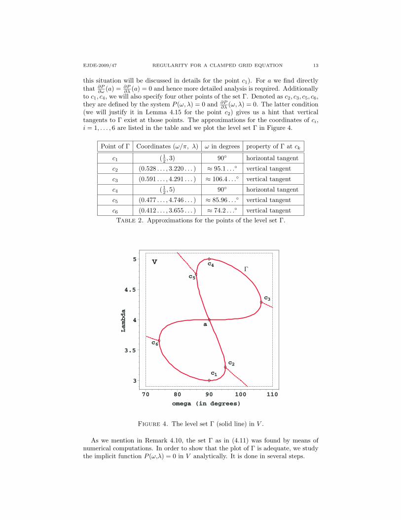
∂λ (ω, λ) = 0. The latter condition(we will justify it in Lemma 4.15 for the point c2) gives us a hint that verticaltangents to Γ exist at those points. The approximations for the coordinates of ci,i = 1, . . . , 6 are listed in the table and we plot the level set Γ in Figure 4.

Point of Γ Coordinates (ω/π, λ) ω in degrees property of Γ at ck

c1 ( 12 , 3) 90 horizontal tangent

c2 (0.528 . . . , 3.220 . . . ) ≈ 95.1 . . . vertical tangent


c4 ( 12 , 5) 90 horizontal tangent


c6 (0.412 . . . , 3.655 . . . ) ≈ 74.2 . . . vertical tangentTable 2. Approximations for the points of the level set Γ.

V

6c

5c

4c

3c

2c

1c

a

3

3. 5

4

4. 5

5

Lambda

7 0 8 0 9 0 10 0 110


Figure 4. The level set Γ (solid line) in V .

As we mention in Remark 4.10, the set Γ as in (4.11) was found by means ofnumerical computations. In order to show that the plot of Γ is adequate, we studythe implicit function P (ω,λ) = 0 in V analytically. It is done in several steps.


The first lemma studies P (ω,λ) = 0 in the vicinity of the point

a = (12π, 4) ∈ Γ. (4.12)

Lemma 4.11. Let U = I × J ⊂ V be the closed rectangle with I =[

88180π,

92180π

],

J = [3.940, 4.060] and let point a ∈ U be as in (4.12). The set Γ given by (4.11)consists of two smooth branches passing through a. Their tangents at a are λ = 4and λ = − 16

√2

π ω + 4.

Proof. Let DP stand for the gradient vector and D2P is the Hessian matrix. Forthe given a we already know that DP (a) = 0. We also find

∂2P∂ω2 (a) = 0, ∂2P

∂ω∂λ (a) = −8√

2π, ∂2P∂λ2 (a) = −π2.

That is, detD2P (a) = −128π2 and by Proposition 8.5 and remark 8.6 (Appendix8) it holds that

P (ω, λ) = − 12h2(ω, λ)

(16√

2h1(ω, λ) + πh2(ω, λ))

on U, (4.13)

where h1, h2 ∈ C∞ (U,R) are given by almost explicit formulas in (8.13), (8.14) inthe same lemma. We also have that h1(a) = h2(a) = 0 and

∂h1∂ω (a) = 1, ∂h1

∂λ (a) = 0, (4.14)∂h2∂ω (a) = 0, ∂h2

∂λ (a) = 1. (4.15)

Due to (4.13) we deduce that in U :

P (ω, λ) = 0 if and only if h2(ω, λ) = 0 or 16√

2h1(ω, λ)+πh2(ω, λ) = 0. (4.16)

By applying the Implicit Function Theorem to the functions h2(ω, λ) = 0 and16√

2h1(ω, λ) + πh2(ω, λ) = 0 in U one finds a parametrization ω 7→ λ = η(ω) foreach of these implicit functions. Indeed:

(1) For h2(ω, λ) = 0 it is shown in Lemma 8.8 (Appendix 8) that∂h2∂λ (ω, λ) > 0 on U,

and hence there exists η1 : I → J , η1 ∈ C∞(I) such that

h2(ω, η1(ω)) = 0,

andη′1(ω) = −∂h2

∂ω (ω, η1(ω))[

∂h2∂λ (ω, η1(ω))

]−1,

for all ω ∈ I. We have that η1( 12π) = 4 and due to (4.15) we find η′1(

12π) = 0.

Hence, there is a smooth branch of Γ in U passing through a, which is given byλ = η1(ω) with the tangent λ = 4.

(2) For 16√

2h1(ω, λ) + πh2(ω, λ) = 0 it is shown in Lemma 8.9 (Appendix 8)that

16√

2∂h1∂λ (ω, λ) + π ∂h2

∂λ (ω, λ) > 0 on U,

and hence there exists η2 : I → J , η2 ∈ C∞(I), where I ⊂ I, such that

16√

2h1 (ω, η2(ω)) + πh2 (ω, η2(ω)) = 0,

and

η′2(ω) = −16√

2∂h1∂ω (ω, η2(ω)) + π ∂h2

∂ω (ω, η2(ω))

16√

2∂h1∂λ (ω, η2(ω)) + π ∂h2

∂λ (ω, η2(ω)),


for all ω ∈ I. We have that η2( 12π) = 4 and due to (4.14) and (4.15) we obtain

η′2(12π) = − 16

√2

π .

Hence, there is another smooth branch of Γ in U passing through a and given byλ = η2(ω). The tangent is λ = − 16

√2

π ω + 4.

The next lemma studies P (ω,λ) = 0 locally in V but away from the point a.

Lemma 4.12. Let

H1 = (ω, λ) : [ 84180π,

90180π]× [4.030, 4.970],

H2 = (ω, λ) : [ 87180π,

101180π]× [4.750, 5.100],

H3 = (ω, λ) : [ 100180π,108180π]× [4.000, 4.850],

H4 = (ω, λ) : [ 91180π,

102180π]× [3.950, 4.100],

H5 = (ω, λ) : [ 90180π,

96180π]× [3.030, 3.970],

H6 = (ω, λ) : [ 79180π,

94180π]× [2.900, 3.230],

H7 = (ω, λ) : [ 72180π,

80180π]× [3.150, 4.000],

H8 = (ω, λ) : [ 78180π,

89180π]× [3.900, 4.050],

and U be as in Lemma 4.11. Then ∪8j=1Hj covers the set Γ in V (see Figure 5)

and in each Hj the following holds:

Rectangle Property in Hj The set Γ in Hj is given by

H2k−1∂P∂ω (ω, λ) 6= 0 ω = φ2k−1(λ) : φ2k−1 ∈ C∞(J2k−1)

H2k∂P∂λ (ω, λ) 6= 0 λ = ψ2k(ω) : ψ2k ∈ C∞(I2k)

Here k = 1, . . . , 4.

Proof. In Claims 8.10 – 8.17 of Appendix 8 we constructed the rectangles Hj ⊂ V ,j = 1, . . . , 8 such that the results of the second column in a table above hold.In Figure 5 we sketched the covering of the set Γ in V with the rectangles Hj ,j = 1, . . . , 8.

Due to result of the second column we can apply the Implicit Function Theoremto the function P (ω,λ) = 0 in everyHj , j = 1, . . . , 8 in order to obtain ω = φ2k−1(λ)or λ= ψ2k(ω), k = 1, . . . , 4. By assumption P∈ C∞(V,R) and hence φ, ψ are C∞

on the corresponding intervals J, I.

Based on the results of the two lemmas above, we arrive at the following result.

Proposition 4.13. The set Γ given by (4.11) is an 8-shaped curve. That is, thereexists an open set V ⊃ [−1, 1]2 and a C∞-diffeomorphism S : V → V such that

S (Γ) = (sin(2t), sin(t)), 0 ≤ t < 2π .

Henceforth, we will call the set Γ a curve (having one self-intersection point)which means that every part of the set Γ is locally parametrizable in ω or λ.


V

a8H

7H

6H

5H

4H

3H

2H

1H

U

3

3. 5

4

4. 5

5

Lambda

70 80 9 0 10 0 110


Figure 5. For lemma 4.12.

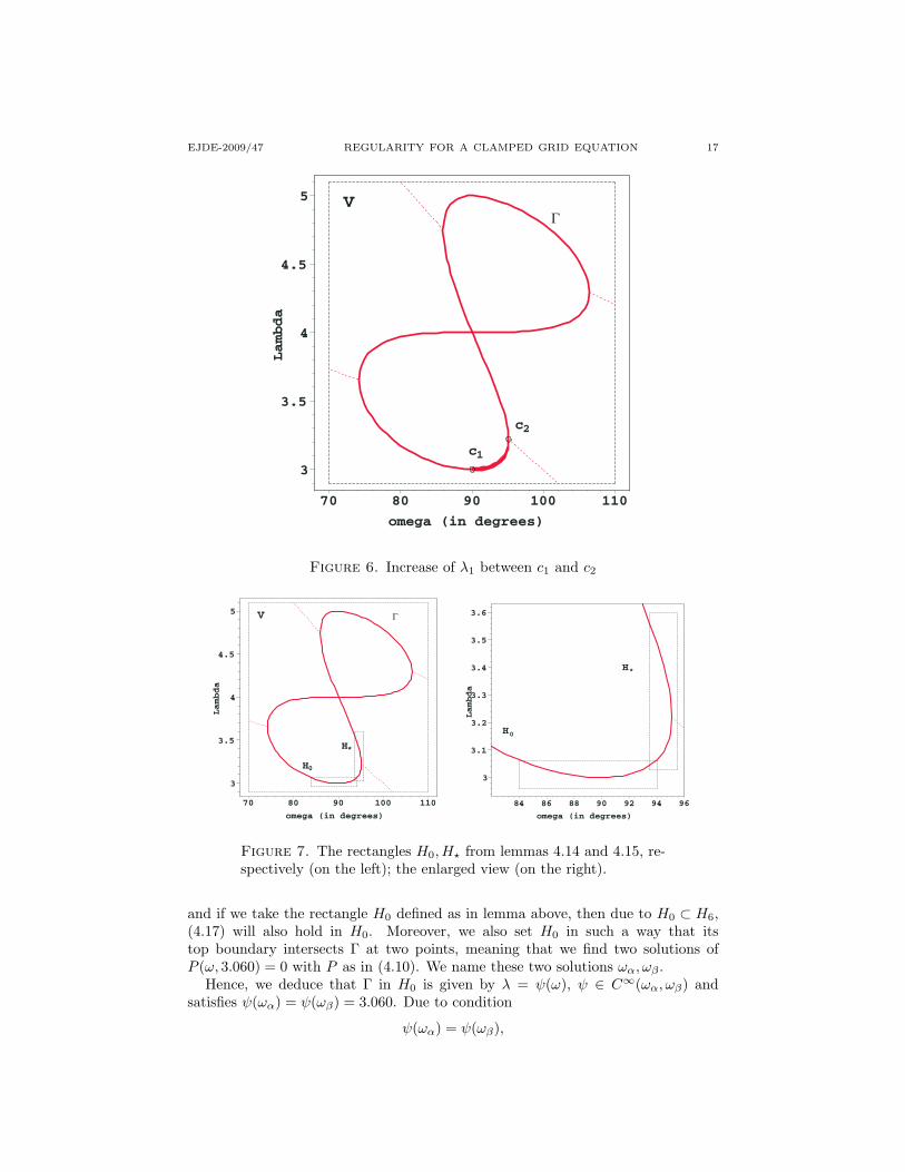
4.4.2. Eigenvalue λ1 as the bottom part of Γ. The curve Γ in a rectangle V combinesthe graphs of the first four eigenvalues λ1, . . . , λ4 of the boundary value problem (4.4) as functions of ω as far as they are real. Here we focus on the eigenvalue λ1

which is a bottom part of Γ (the segment c6c1c2 ⊂ Γ in Figure 4). In particular,we prove that as a function of ω the eigenvalue λ1 = λ1(ω) increases between thepoints c1, c2 (the approximations for their coordinates are given in Table 2). Thesituation is illustrated by Figure 6.

To prove this result, we follow the approach used in Lemmas 4.11 and 4.12.To be more precise, we fix two rectangles H0,H? ⊂ V such that H0 ∩ H? 6= ∅and H0 ∪H? covers the part of Γ containing the segment c1c2 (see Figure 7). Weparameterize Γ in H0,H? as ω 7→ λ = ψ(ω) and λ 7→ ω = ϕ(λ), respectively,and study the properties of these parametrizations (convexity-concavity, extremumpoints, the intervals of increase-decrease). This will enable to gain the informationabout c1c2.

Lemma 4.14. Let H0 = I0×J0 ⊂ V be the closed rectangle with I0 =[

84180π,

94180π

]and J0 = [2.960, 3.060]. It holds that Γ in H0 is given by λ = ψ(ω), ψ ∈ C∞(ωα, ωβ),(ωα, ωβ) ⊂ I0 and is such that it attains its minimum on (ωα, ωβ) at ω = ω0 = 1

2πand increases monotonically on (ω0, ωβ). Here ωα, ωβ are the solutions to the equa-tion P (ω, 3.060) = 0 on ω ∈

(84180π,

12π

)and on ω ∈

(12π,

94180π

), respectively, with

P given by (4.10).

Proof. By Lemma 4.12 we know that

P (ω, λ) = 0 if and only if P (ω, ψ(ω)) = 0 in H6, (4.17)


V

2c

1c

3

3. 5

4

4. 5

5

Lambda

7 0 8 0 9 0 10 0 110


Figure 6. Increase of λ1 between c1 and c2

V

0H

*H

3

3. 5

4

4. 5

5

Lambda

7 0 8 0 9 0 1 00 1 1 0


0H

*H

3

3. 1

3. 2

3. 3

3. 4

3. 5

3. 6

Lambda

8 4 8 6 8 8 9 0 9 2 9 4 9 6


Figure 7. The rectangles H0,H? from lemmas 4.14 and 4.15, re-spectively (on the left); the enlarged view (on the right).

and if we take the rectangle H0 defined as in lemma above, then due to H0 ⊂ H6,(4.17) will also hold in H0. Moreover, we also set H0 in such a way that itstop boundary intersects Γ at two points, meaning that we find two solutions ofP (ω, 3.060) = 0 with P as in (4.10). We name these two solutions ωα, ωβ .

Hence, we deduce that Γ in H0 is given by λ = ψ(ω), ψ ∈ C∞(ωα, ωβ) andsatisfies ψ(ωα) = ψ(ωβ) = 3.060. Due to condition

ψ(ωα) = ψ(ωβ),


by Rolle’s theorem there exists ω0 ∈ (ωα, ωβ) such that ψ′(ω0) = 0.Since P (ω0, ψ (ω0)) = 0 and due to

ψ′(ω) = −∂P∂ω (ω, ψ(ω))[∂P

∂λ (ω, ψ(ω))]−1,

we solve the system P (ω, λ) = 0 and ∂P∂ω (ω, λ) = 0 in H0 in order to find ω0. Its

solution is a point c1 = (12π, 3) and hence

ω0 = 12π.

We deduce that λ = ψ(ω) attains its local extremum at ω = ω0.Next we show that λ = ψ(ω) has a minimum at ω = ω0 on (ωα, ωβ). For this

purpose we consider a function G ∈ C∞(H0,R) such that

G (ω, ψ(ω)) = ψ′′(ω). (4.18)

For an explicit formula for G see Appendix 8. In Claim 8.18 of this Appendix weshow that

G(ω, λ) > 0 on H0. (4.19)This condition together with (4.18) yields

G (ω, ψ(ω)) = ψ′′(ω) > 0 on (ωα, ωβ),

meaning that λ = ψ(ω) is convex on (ωα, ωβ).The result is that λ = ψ(ω) attains its minimum on (ωα, ωβ) at ω = ω0 = 1

2πand increases monotonically on the interval ω ∈ (ω0, ωβ).

We also have the following result.

Lemma 4.15. Let H? = I?×J? ⊂ V be the closed rectangle with I? =[93.5180 π,

95.5180 π

]and J? = [3.030, 3.600]. It holds that Γ in H? is given by ω = ϕ(λ), ϕ ∈ C∞(λγ , λδ),(λγ , λδ) ⊂ J? and is such that it attains its maximum on (λγ , λδ) at λ = λ? ≈3.220 . . . and increases monotonically on the interval (λγ , λ?). Here λγ , λδ arethe solutions to the equation P

(93.5180 π, λ

)= 0 on λ ∈ (3.030, 3.100) and on λ ∈

(3.500, 3.600), respectively. Also, λ? is the solution to the system P (ω, λ) = 0 and∂P∂λ (ω, λ) = 0 on λ ∈ (λγ , λδ); P given by (4.10).

Proof. By Lemma 4.12 we know that

P (ω, λ) = 0 if and only if P (ϕ(λ), λ) = 0 in H5, (4.20)

and if we take the rectangle H? defined as in lemma above, then due to H? ⊂ H5,(4.20) will also hold in H?. Moreover, we also set H? in such a way that its leftboundary intersects Γ at two points, meaning we find two solutions of P

(93.5180 π, λ

)=

0 with P as in (4.10). We name these two solutions λγ , λδ.Hence, we deduce that Γ in H? is given by ω = ϕ(λ), ϕ ∈ C∞(λγ , λδ) and

satisfies ϕ(λγ) = ϕ(λδ) = 93.5180 π. Due to condition

ϕ(λγ) = ϕ(λδ),

by Rolle’s theorem there exists λ? ∈ (λγ , λδ) such that ϕ′(λ?) = 0.Since P (ϕ(λ?), λ?) = 0 and due to

ϕ′(λ) = −∂P∂λ (ϕ(λ), λ)[∂P

∂ω (ϕ(λ), λ)]−1,

we solve the system P (ω, λ) = 0 and ∂P∂λ (ω, λ) = 0 in H? in order to find λ?. Its

solution is a point c2 =(ω, λ

), where ω/π ≈ 0.528 . . . and λ ≈ 3.220 . . . . Hence,

λ? ≈ 3.220 . . . .


We deduce that ω = ϕ(λ) attains its local extremum at λ = λ?.Next we show that ω = ϕ(λ) has a maximum at λ = λ? on (λγ , λδ). For this

purpose we consider a function F ∈ C∞ (H?,R) such that

F (ϕ(λ), λ) = ϕ′′(λ). (4.21)

For explicit formula for F see Appendix 8. In Claim 8.19 of this Appendix we showthat

F (ω, λ) < 0 on H?. (4.22)This condition together with (4.21) yields

F (ϕ(λ), λ) = ϕ′′(λ) < 0 on (λγ , λδ),

meaning that ω = ϕ(λ) is concave on (λγ , λδ). The result is that ω = ϕ(λ) attainsits maximum on (λγ , λδ) at λ = λ? ≈ 3.220 . . . and increases monotonically on theinterval λ ∈ (λγ , λ?).

Theorem 4.16. As a function of ω the first eigenvalue λ1 = λ1(ω) of the boundaryvalue problem (4.4) increases on ω ∈

(12π, ω?

). Here ω?/π ≈ 0.528 . . . (in degrees

ω? ≈ 95.1 . . .) and λ? ≈ 3.220 . . . .

4.5. The multiplicities of λj∞j=1 and the structure of a singular solution.Here we proceed with the qualitative analysis of the eigenvalues λj∞j=1 of problem(4.4).

Definition 4.17. Let ω ∈ (0, 2π] be fixed. The eigenvalue λj , j ∈ N+ of problem(4.4) is said to have an algebraic multiplicity κ(j) ≥ 1, if the following holds:

P (ω, λj) = 0, dPdλ (ω, λj) = 0, . . . , dκ(j)−1P

dλκ(j)−1(ω, λj) = 0, dκ(j)

P

dλκ(j) (ω, λj) 6= 0.

Based on the numerical approximations for some first eigenvalues λj , j ∈ N+

depicted in Figure 3 (the top one) and partly by our derivations (namely, theexistence of the solution to the system P (ω, λ) = ∂P

∂λ (ω, λ) = 0 in Lemma 4.15) webelieve that the maximal algebraic multiplicity of a certain λj of problem (4.4) isat most 2 . Indeed, generically 3 curves never intersect at one point, meaning thatgeometrically the algebraic multiplicity will always be at most 2.

Definition 4.18. The eigenvalue λj , j ∈ N+ of problem (4.4) is said to have ageometric multiplicity I(j) ≥ 1, if the number of linearly independent eigenfunctionsΦ equals I(j).

For given λj , j ∈ N+ of problem (4.4) the three cases occur:1. κ(j) = I(j) = 1 one finds a solution (λj ,Φ

(j)0 ) of (4.4) and then the solution

of (4.1) reads:u

(j)0 = rλj+1Φ(j)

0 (θ); (4.23)

2. κ(j) = 2, I(j) = 1 one finds a solution (λj ,Φ(j)0 ) of (4.4) and a generalized

solution (λj ,Φ(j)1 ), with Φ(j)

1 found from the equation

L(λj)Φ(j)1 + L′(λj)Φ

(j)0 = 0,

where L(λ) is given by (4.3) and L′(λ) = ddλL(λ). Then we have two solutions of

(4.1):

u(j)0 = rλj+1Φ(j)

0 (θ) and u(j)1 = rλj+1

(Φ(j)

1 (θ) + log(r)Φ(j)0 (θ)

); (4.24)


3. κ(j) = I(j) = 2 one finds two solutions (λj ,Φ(j)0 ), (λj ,Φ

(j)1 ) of (4.4), where

Φ(j)0 and Φ(j)

1 are linearly independent on θ ∈ (0, ω) and then we again have twosolutions of (4.1):

u(j)0 = rλj+1Φ(j)

0 (θ) and u(j)1 = rλj+1Φ(j)

1 (θ). (4.25)

Let us note that for an opening angle ω ∈ 12π, π,

32π, 2π of the sector Kω

one can find the eigenvalues λj∞j of the problem (4.4) explicitly. Moreover, ifω ∈

12π, π

, then for every given λj one can compute explicitly the corresponding

eigenfunctions Φ(j)q , q = 0, . . . , κ(j)−1, whereas if ω ∈

32π, 2π

, the eigenfunctions

Φ(j)q can be computed explicitly only for some λj . Thus, in Appendix 9 we bring the

formulas of some first functions Φ(j)q (if computable) and the respective solutions

u(j)q to (4.1).These functions rλ+1Φ(θ) and rλ+1 log(r)Φ(θ) determine the bands for the reg-

ularity in Kondratiev’s theory. Details are found in the next section.

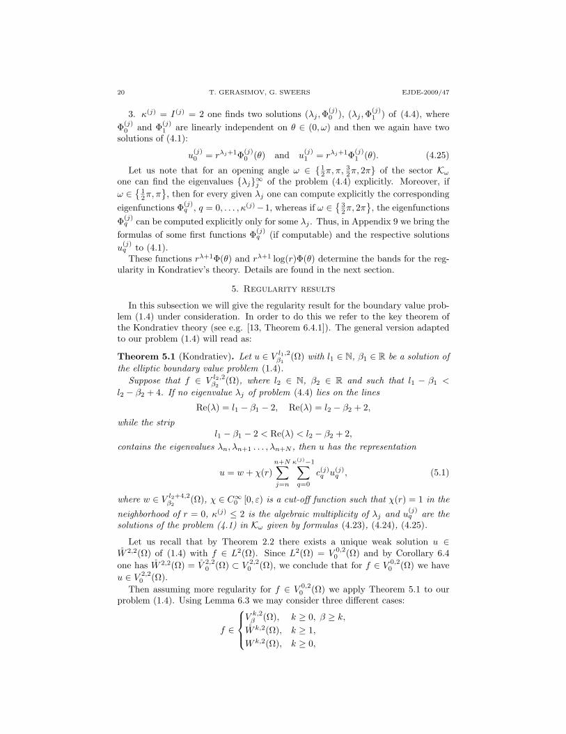
5. Regularity results

In this subsection we will give the regularity result for the boundary value prob-lem (1.4) under consideration. In order to do this we refer to the key theorem ofthe Kondratiev theory (see e.g. [13, Theorem 6.4.1]). The general version adaptedto our problem (1.4) will read as:

Theorem 5.1 (Kondratiev). Let u ∈ V l1,2β1

(Ω) with l1 ∈ N, β1 ∈ R be a solution ofthe elliptic boundary value problem (1.4).

Suppose that f ∈ V l2,2β2

(Ω), where l2 ∈ N, β2 ∈ R and such that l1 − β1 <

l2 − β2 + 4. If no eigenvalue λj of problem (4.4) lies on the lines

Re(λ) = l1 − β1 − 2, Re(λ) = l2 − β2 + 2,

while the stripl1 − β1 − 2 < Re(λ) < l2 − β2 + 2,

contains the eigenvalues λn, λn+1 . . . , λn+N , then u has the representation

u = w + χ(r)n+N∑j=n

κ(j)−1∑q=0

c(j)q u(j)q , (5.1)

where w ∈ V l2+4,2β2

(Ω), χ ∈ C∞0 [0, ε) is a cut-off function such that χ(r) = 1 in the

neighborhood of r = 0, κ(j) ≤ 2 is the algebraic multiplicity of λj and u(j)q are the

solutions of the problem (4.1) in Kω given by formulas (4.23), (4.24), (4.25).

Let us recall that by Theorem 2.2 there exists a unique weak solution u ∈W 2,2(Ω) of (1.4) with f ∈ L2(Ω). Since L2(Ω) = V 0,2

0 (Ω) and by Corollary 6.4one has W 2,2(Ω) = V 2,2

0 (Ω) ⊂ V 2,20 (Ω), we conclude that for f ∈ V 0,2

0 (Ω) we haveu ∈ V 2,2

0 (Ω).Then assuming more regularity for f ∈ V 0,2

0 (Ω) we apply Theorem 5.1 to ourproblem (1.4). Using Lemma 6.3 we may consider three different cases:

f ∈

V k,2

β (Ω), k ≥ 0, β ≥ k,

W k,2(Ω), k ≥ 1,W k,2(Ω), k ≥ 0,


and obtain the following result (in order to describe all three cases and also for theconvenience we arranged this result as a table):

Theorem 5.2. Let f ∈ L2(Ω) and let u ∈ W 2,2(Ω) be a weak solution to (1.4).

f is in V k,2β (Ω), k ≥ 0, β ≥ k W k,2(Ω), k ≥ 1 W k,2(Ω), k ≥ 0

no eigenvalueλj of (4.4) lieson the lines

Re(λ) = 0,Re(λ) = k − β + 2

Re(λ) = 0,Re(λ) = k + 2

Re(λ) = 0,Re(λ) = 2

while the strip 0 < Re(λ) < k − β + 2 0 < Re(λ) < k + 2 0 < Re(λ) < 2

contains λ1, λ2, . . . , λN

u = w + χ(r)∑N

j=1

∑κ(j)−1q=0 c

(j)q u

(j)q

where w is in V k+4,2β (Ω) W k+4,2(Ω) W k+4,2(Ω, |x|2kdµ)

and χ ∈ C∞0 [0, ε) is a cut-off function such that χ = 1 in the neighborhood of r = 0,

κ(j) ≤ 2 is the algebraic multiplicity of λj and u(j)q are the solutions of the problem

(4.1) in Kω given by formulas (4.23), (4.24), (4.25).

Remark 5.3. The first column gives the optimal regularity in the sense of Kon-dratiev’s spaces. The second and third column shows two corollaries with the morecommonly used Sobolev spaces. Away from the corner also these results are opti-mal. Of course the optimal regularity near a corner can not be stated using justthe standard Sobolev spaces W `,2(Ω).

Proof of Theorem Theorem2. The first column is just a representation of the previ-ous theorem in the case that f ∈ L2(Ω) and a weak solution u ∈ W 2,2(Ω) is knownto exist. Additional regularity in the sense of Kondratiev’s weighted Sobolev spacesfor f implies the representation as stated for the solution u. In the second and thirdcolumn the most common special cases are listed independently. For the secondcolumn one uses the imbeddings

W k,2(Ω) ⊂ V k,20 (Ω) and V k+4,2

0 (Ω) ⊂W k+4,2(Ω),

and for the third

W k,2(Ω) ⊂ V k,2k (Ω) and V k+4,2

k (Ω) ⊂W k+4,2(Ω, |x|2kdµ).

As the last step of our analysis we derive the regularity in Ω for the singular part∑Nj=1

∑κ(j)−1q=0 c

(j)q u

(j)q of the solution u given in Theorem 5.2.

5.1. Regularity for the singular part of u. The first term of the summation∑Nj=1

∑κ(j)−1q=0 c

(j)q u

(j)q in the solution u defines the regularity of the whole sum.

From formulas (4.23), (4.24), (4.25) we know that depending on the algebraic mul-tiplicity of λ1 it reads as

rλ1+1Φ(θ) or rλ1+1 (Ψ(θ) + log(r)Φ(θ)) ,

where λ1 ∈ C is the first eigenvalue of (4.4) such that Re(λ1) > 0 and Φ(θ),Ψ(θ) ∈C∞[0, ω], 0 < ω < 2π.


Lemma 5.4. Let Φ(θ) ∈ C∞[0, ω] be nontrivial and 0 < ω < 2π. Let also λ ∈ C\Zwith Re(λ) > 0. Suppose that k ∈ 0, 1, 2, 3, . . . . Then the following are equivalent:

(1) rλ+1Φ(θ) ∈W k,2(Ω),(2) rλ+1 log(r)Φ(θ) ∈W k,2(Ω),(3) Re(λ) + 1 > k − 1.

Proof. If λ is not an integer, then the first item and second items are equivalent withan integrability condition for the kth -derivative that reads as 2Re(λ+1−k)+1 >−1.

Remark 5.5. To restrict the already heavy technical aspects we have not consid-ered (weighted) Sobolev spaces with non-integer coefficients k and Holder spaces.A similar result will hold for k is noninteger. Concerning Holder spaces:

rλ+1Φ(θ) ∈ Ck,γ(Ω) for Re(λ) + 1 ≥ k + γ with k ∈ N, γ ∈ [0, 1).

For the second function it holds that

rλ+1 log(r)Φ(θ) ∈ Ck,γ(Ω) for Re(λ) + 1 > k + γ with k ∈ N, γ ∈ [0, 1).

A useful consequence of the above lemma is that for every fixed λ ∈ C withRe(λ) > 0 we deduce

rλ+1Φ(θ), rλ+1 log(r)Φ(θ)∈W dRe(λ)e+1,2(Ω), (5.2)

where d·e stands for the ceiling function (defined as dxe = minn ∈ Z : x ≤ n).

Remark 5.6. In the particular cases, namely, ω = 12π and ω = π we know that

each term u(j)q of the singular part

∑Nj=1

∑κ(j)−1q=0 c

(j)q u

(j)q is a polynomial in x, y of

order λj + 1 (see Appendix 9). That is, for every λj , j ∈ N+ we have

rλj+1Φ(j)(θ) = Pλj+1(x, y) ∈ C∞ (Ω

). (5.3)

For non-polynomials the result in Lemma 5.4 even holds for λ ∈ N.

Now, in order to use the result of Lemma 5.4, we proceed with Figure 8 wherewe plot the Re(λ1) as a function of the opening angle ω on the interval ω ∈ (0, 2π].The two cases are compared: the plots of Re(λ1) of the boundary value problem(4.4) for L related to L = ∂4

∂x4 + ∂4

∂y4 and L = ∆2. In Figure 9 we split the plot ofFigure 8 into two: a plot of Re(λ1) on ω ∈ (0, π] and ω ∈ [π, 2π].

Based on the numerical approximations to λ1 and partly on the analytical esti-mates for λ1 we conclude the following.

Claim 5.7. (0, 2π] 3 ω 7→ Re(λ1(ω)) is a continuous function and

for ω ∈ (0, ω1)/12π : Re(λ1) > 3, for ω =

12π : Re(λ1) = 3,

for ω ∈ [ω1, ω2) : 3 ≥ Re(λ1) > 2, for ω ∈ [ω2, π) : 2 ≥ Re(λ1) > 1,

for ω ∈ [π, 2π] : 1 ≥ Re(λ1) ≥12.

Here ω1, ω2 are respectively the solutions of P (ω, 3 + iξ) = 0 on ω ∈(

12π,

120180π

)and of P (ω, 2 + iξ) = 0 on ω ∈

(23π,

34π

), where P as in formula (4.7) for ` = 1

. The approximation are ω1/π ≈ 0.555 . . . (in degrees ω1 ≈ 99.9 . . .) and ω2/π ≈0.720 . . . (in degrees ω2 ≈ 129.7 . . .).


Bilaplacian

G r id o pe r at o r

0

1

2

3

4

5

6

7

Re(Lambda)

0 50 100 150 200 250 300 350

o m e g a ( in d e g r e e s )

Figure 8. The plot of eigenvalue λ1 in (ω,Re(λ)) ∈ (0, 2π] ×[0, 7.200] of problem ( 4.4). For L related to ∂4

∂x4 + ∂4

∂y4 , λ1 isrepresented by the red line and for L related to ∆2, by the blueline. Dashed lines depict the real part of λ1 ∈ C, solid lines are forpurely real λ1; the vertical lines mark out

12π, π,

32π, 2π

on ω-

axis.

5.2. Consequences. For the numerical results from Claim 5.7, it holds by Theo-rem 5.2 that:

Corollary 5.8. Let u ∈ W 2,2(Ω) be a weak solution of problem (1.4) with f ∈L2(Ω). Then

for ω ∈ (0, ω2) : u ∈W 4,2(Ω), for ω ∈ (ω2, π) : u ∈W 3,2(Ω),

for ω = π : u ∈W 4,2(Ω), for ω ∈ (π, 2π] : u ∈W 2,2(Ω).

Here ω2 is as in Claim 5.7.

Remark 5.9. For the opening angle ω = ω2 we have Re(λ1) = 2 and henceTheorem 5.2 does not apply. Nevertheless, assuming f ∈ L2(Ω) to be more regular,e.g. in V 1,2

0 (Ω) or W 1,2(Ω), we may show that

for ω = ω2 : u ∈W 3,2(Ω).

Proof. By Theorem 5.2 if f ∈ L2(Ω), the solution u of problem (1.4) reads as

u = w + χ(r)∑

0<λj<2

κ(j)−1∑q=0

c(j)q u(j)q , (5.4)

with w ∈ W 4,2(Ω). Due to 5.7 we see that the sum in ( 5.4) has no terms whenω ∈ (0, ω2) and hence for ω ∈ (0, ω2) we have u ∈W 4,2(Ω).

For ω ∈ (ω2, π)∪(π, 2π] the first term of sum in (5.4), depending on the algebraicmultiplicity of λ1, reads as u(1)

0 = rλ1+1Φ(1)0 (θ), or as a linear combination of


Bilaplacian


1

2

3

4

5

6

7

Re(Lambda)

0 50 10 0 150


Bilaplacian


0 . 5

1

Re(Lambda)

2 0 0 2 5 0 3 0 0 3 5 0


Figure 9. The plot of Figure 8 rescaled. The curves for the grid-operator and the bilaplacian intersect four times. Three of thesepoints (we obviously exclude ω = π) seem to be special: It lookslike the curves intersect at ω = 3

4π, ω = 54π and ω = 7

4π (the inter-section points are marked by cross). The numerical approximationshows however that the first values λ1,Grid and λ1,Bilaplace at thosepoints only coincide up to three digits.

u(1)0 = rλ1+1Φ(1)

0 (θ) and u(1)1 = rλ1+1

(Φ(1)

1 (θ) + log(r)Φ(1)0 (θ)

). By (5.2) we have

thatu

(1)0 , u

(1)1

∈ W dRe(λ)e+1,2(Ω), where due to Claim 5.7 we may deduce that


dRe(λ1)e+ 1 = 3, when ω ∈ (ω2, π) and dRe(λ1)e+ 1 = 2, when ω ∈ (π, 2π]. Thisresults in u ∈W 3,2(Ω) for ω ∈ (ω2, π) and u ∈W 2,2(Ω) for ω ∈ (π, 2π].

Finally, for ω = π due to (5.3) the singular part is of C∞(Ω) and hence u ∈W 4,2(Ω) in this case.

6. Comparing (weighted) Sobolev spaces

6.1. One-dimensional Hardy-type inequalities.

Lemma 6.1 (A higher order one-dimensional Hardy inequality). Let w be a func-tion in C∞

0 [x1, x2]. For every k ≥ 1 it holds that∫ x2

x1

(w(x)

(x−x1)k

)2

dx = 4k

(2k−1)2(2k−3)2...3212

∫ x2

x1

(w(k)(x)

)2

dx. (6.1)

Proof. It holds straightforwardly that∫ x2

x1

(w(x)

(x−x1)k

)2

dx

=1

1− 2k

[(w(x))2 (x− x1)1−2k

]|x2x1

+2

2k − 1

∫ x2

x1

w(x)w′(x)(x− x1)1−2kdx

≤ 22k − 1

( ∫ x2

x1

(w(x)

(x−x1)k

)2

dx)1/2( ∫ x2

x1

(w′(x)

(x−x1)k−1

)2

dx)1/2

and the first step in the proof of (6.1) follows. Repeating the argument for w′ andk − 1 etc. will give the result.

Remark 6.2. Since W k,2(x1, x2), k ≥ 1 is the closure of C∞0 [x1, x2] in the W k,2-

norm, one can use the results of Lemma 6.1 for every w ∈ W k,2(x1, x2), k ≥ 1.

6.2. Imbeddings. As mentioned e.g. in [12, page 240] or [13, Chapter 7, sum-mary], the family of weighted spaces V l,2

β does not contain the ordinary Sobolev

spaces without weight. More precisely: W k,2 /∈V l,2

β

l,β

for k ≥ 1. We will prove

the imbedding results for bounded Ω that satisfy Condition 1.1.

Lemma 6.3. Let β ∈ R and l ∈ 0, 1, 2, . . . . Then the following holds:

(a) V l,2β (Ω) ⊂W l,2(Ω) if and only if β ≤ 0,

(b) W l,2(Ω) ⊂ V l,2β (Ω) if and only if β ≥ l,

(c) V l,2β (Ω) ⊂ W l,2(Ω) if and only if β ≤ 0,

(d) W l,2(Ω) ⊂ V l,2β (Ω) if and only if β ≥ 0.

Corollary 6.4. For l ∈ 0, 1, 2, . . . one has

W l,2(Ω) = V l,20 (Ω).

Proof of Lemma 6.3. Let Ω be as in Condition 1.1 and Ω ⊂ BM (0), where BM (0)is an open ball of radius M > 0. The statement in a) goes as follows: for (x, y) ∈ Ωone has 0 ≤ r ≤M and hence r2(β−l+|α|) ≥M2(β−l+|α|) if and only if β−l+|α| ≤ 0.Since 0 ≤ |α| ≤ l, we obtain β ≤ 0. This enables us to have the estimate

‖u‖V l,2β (Ω) =

( l∑|α|=0

∫Ω

r2(β−l+|α|)|Dαu|2dx dy)1/2


≥( l∑|α|=0

∫Ω

M2(β−l+|α|)|Dαu|2dx dy)1/2

≥ min(1,Mβ−l)( l∑|α|=0

∫Ω

|Dαu|2dx dy)1/2

= min(1,Mβ−l)‖u‖W l,2(Ω),

which is the result in (a).To prove the statement in (b) we notice that r2(β−l+|α|) ≤ M2(β−l+|α|) if and

only if β − l + |α| ≥ 0. Due to 0 ≤ |α| ≤ l, we obtain β ≥ l and then the estimateholds

‖u‖V l,2β (Ω) =

( l∑|α|=0

∫Ω

r2(β−l+|α|)|Dαu|2dx dy)1/2

≤( l∑|α|=0

∫Ω

M2(β−l+|α|)|Dαu|2dx dy)1/2

≤ max(1,Mβ−l)( l∑|α|=0

∫Ω

|Dαu|2dx dy)1/2

= max(1,Mβ−l)‖u‖W l,2(Ω).

This is the result in (b).To prove the statements in (c) and (d) we set θ = 1

2ω where the opening angleω ∈ (0, 2π). We also use the fact that for our domain there exists c > 0 such thatr > cρ(x, y), where ρ denotes the distance from a point (x, y) on the lines

` : y = tan(θ)x+ τ,

with τ ∈ R to the point (x1, y1) ∈ ∂Ω. In particular, it holds that

ρ2 = (x− x1)2(1 + tan2(θ)).

We may integrate along the lines ` and use the one-dimensional Hardy-inequalityto find that there exist Cl ∈ R+ with

‖u‖V l,20 (Ω) ≤ Cl‖u‖W l,2(Ω) for all u ∈ C∞

c (Ω). (6.2)

On the other hand, using the same trick as in proof of a) we find Cl ∈ R+ suchthat

Cl‖u‖W l,2(Ω) ≤ ‖u‖V l,20 (Ω) for all u ∈ C∞

c (Ω). (6.3)

Estimates (6.2), (6.3) yield

W l,2(Ω) = V l,20 (Ω).

Due to imbedding V l,2β1

(Ω) ⊂ V l,20 (Ω) ⊂ V l,2

β2(Ω) when β1 ≤ 0 ≤ β2 one obtains the

result in (c) and (d).


0

y

x

)2y,2( x

)1y,1( x

1l

l

Figure 10. Domain Ω with a concave corner ω intersected by `

7. A fundamental system of solutions

7.1. Derivation of system Sλ. Let us find the fundamental set of solutions toequation

L(θ, ddθ , λ)Φ = 0, (7.1)

with L(θ, ddθ , λ) as in formula (4.3). For this L it seems to be hard to derive a set

of functions solving (7.1) explicitly. The following approach applies in this case.For L = ∂4

∂x4 + ∂4

∂y4 we find L(rλ+1Φ

)= rλ−3L

(θ, d

dθ , λ)Φ and hence instead of

L(θ, d

dθ , λ)Φ = 0 we may consider the equation

L(rλ+1Φ

)= 0. (7.2)

Operator L admits the decomposition

L = ∂4

∂x4 + ∂4

∂y4 =2∏

p=1

(∂∂y − τp

∂∂x

) 2∏p=1

(∂∂y + τp

∂∂x

),

with τ1 =√

22 (1+ i), τ2 =

√2

2 (1− i) and hence every function of the form F (x±τpy)solves (7.2). Therefore, we have that

rλ+1Φ(θ) =2∑

p=1

cpfp(x+ τpy) + cp+2fp+2(x− τpy),

and after translation fp, fp+22p=1 into polar coordinates we set

fp (r cos(θ) + τpr sin(θ)) := (r cos(θ) + τpr sin(θ))λ+1,


fp+2 (r cos(θ)− τpr sin(θ)) := (r cos(θ)− τpr sin(θ))λ+1,

So, the set of functions

ϕ1(θ) = (cos(θ) + τ1 sin(θ))λ+1, ϕ2(θ) = (cos(θ) + τ2 sin(θ))λ+1

, (7.3)

ϕ3(θ) = (cos(θ)− τ1 sin(θ))λ+1, ϕ4(θ) = (cos(θ)− τ2 sin(θ))λ+1

, (7.4)is a set of solutions to (7.1). The Wronskian for ϕm4m=1 reads as

W (ϕ1(θ), ϕ2(θ), ϕ3(θ), ϕ4(θ)) = det

ϕ1(θ) ϕ2(θ) ϕ3(θ) ϕ4(θ)ϕ′1(θ) ϕ′2(θ) ϕ′3(θ) ϕ′4(θ)ϕ′′1(θ) ϕ′′2(θ) ϕ′′3(θ) ϕ′′4(θ)ϕ′′′1 (θ) ϕ′′′2 (θ) ϕ′′′3 (θ) ϕ′′′4 (θ)

, (7.5)

and by straightforward computations one finds

W = 16 (λ+ 1)3 λ2 (λ− 1)(cos4(θ) + sin4(θ)

)λ−2,

which is non-zero on θ ∈ (0, 2π] except for λ ∈ ±1, 0. Hence, except for thesevalues ϕm4m=1 given in (7.3), (7.4) is a fundamental system of solutions to (7.1).

7.2. Derivation of systems S−1, S0, S1. Here we find the fundamental systemsof solutions to equation L

(θ, ∂

∂θ , λ)Φ = 0 when λ ∈ ±1, 0. We will go into details

in solving the corresponding equation for every λ ∈ ±1, 0.

7.2.1. Case λ = −1. For λ = −1 the equation (7.1) reads as14 (3 + cos(4θ))Φ′′′′ − 3 sin(4θ)Φ′′′ + (3− 11 cos(4θ))Φ′′ + 12 sin(4θ)Φ′ = 0. (7.6)

First we set Φ(θ) =∫F (θ)dθ and obtain the equation for F :

14 (3 + cos(4θ))F ′′′ − 3 sin(4θ)F ′′ + (3− 11 cos(4θ))F ′ + 12 sin(4θ)F = 0.

The first integral of the above equation reads as14 (3 + cos(4θ))F ′′ − 2 sin(4θ)F ′ + 3(1− cos(4θ))F = c0.

We use the change of variables F (θ) = (3 + cos(4θ))−1G(θ) and get

G′′ + 4G = 4c0.

Solution of the last equation reads as

G(θ) = c1 sin(2θ) + c2 cos(2θ) + c0.

and thenF (θ) = c1

sin(2θ)3+cos(4θ) + c2

cos(2θ)3+cos(4θ) + c3

13+cos(4θ) .

As a result, Φ that solves (7.6) will read as

Φ(θ) = A1 +A2

∫sin(2θ)

3+cos(4θ)dθ +A3

∫cos(2θ)

3+cos(4θ)dθ +A4

∫1

3+cos(4θ)dθ,

and then the candidates that may form the fundamental system of solutions to (7.6)will be the following:

ϕ1(θ) = 1,

ϕ2(θ) = −4∫

sin(2θ)3+cos(4θ)dθ = arctan (cos(2θ)) ,

ϕ3(θ) = 4√

2∫

cos(2θ)3+cos(4θ)dθ = arctanh

(√2

2 sin(2θ)),


ϕ4(θ) = 4√

2∫

13+cos(4θ)dθ =

arctan

(√2

2 tan(2θ))

+ `π, θ ∈(

2`−14 π, 2`+1

4 π),

2θ θ = 2`+14 π,

with ` = 0, . . . , 4. Formula for ϕ4 is given on the interval θ ∈(− 1

4π, 2π + 14π

)in

order to have the concise explicit form.The Wronskian W of ϕ1, . . . , ϕ4 is proportional to

(cos4(θ) + sin4(θ)

)−3and is

non-zero on θ ∈ (0, 2π]. Hence, ϕm4m=1 defined as above is a fundamental systemof solutions to (7.6).

7.2.2. Case λ = 0. For λ = 0 the equation (7.1) reads as:14 (3 + cos(4θ))Φ′′′′ − 2 sin(4θ)Φ′′′ + 1

2 (3− 7 cos(4θ))Φ′′

− 2 sin(4θ)Φ′ + 34 (1− 5 cos(4θ))Φ = 0,

(7.7)

and can be split as follows:(d2

dθ2 + 1) (

14 (3 + cos(4θ))

(d2

dθ2 + 1))

Φ = 0.

So, Φ solvesΦ′′ + Φ = A sin(θ)

3+cos(4θ) +B cos(θ)3+cos(4θ) ,

and after integrating this equation we obtain

Φ(θ)

= A1 sin(θ) +A2 cos(θ) +A3

(12 sin(θ) arctan (cos(2θ)) + 4 cos(θ)

∫ θ

0

sin2(y)3+cos(4y)dy

)+A4

(12 cos(θ) arctan (cos(2θ)) + 4 sin(θ)

∫ θ

0

cos2(y)3+cos(4y)dy

).

The candidates that may form the fundamental system of solutions to (7.7) will bethe following:

ϕ1(θ) = sin(θ), ϕ2(θ) = cos(θ),

ϕ3(θ) = 12 sin(θ) arctan (cos(2θ)) + 4 cos(θ)

∫ θ

0

sin2(y)3+cos(4y)dy,

ϕ4(θ) = 12 cos(θ) arctan (cos(2θ)) + 4 sin(θ)

∫ θ

0

cos2(y)3+cos(4y)dy.

The Wronskian W of ϕ1, . . . , ϕ4 is proportional to(cos4(θ) + sin4(θ)

)−2and is non-

zero on θ ∈ (0, 2π]. Hence, ϕm4m=1 defined as above is a fundamental system ofsolutions to (7.7).

7.2.3. Case λ = 1. For λ = 1 the equation (7.1) reads as:14 (3 + cos(4θ))Φ′′′′ − sin(4θ)Φ′′′ + (3 + cos(4θ))Φ′′ − 4 sin(4θ)Φ′ = 0. (7.8)

We set Φ(θ) =∫F (θ)dθ and obtain the equation for F :

14 (3 + cos(4θ))F ′′′ − sin(4θ)F ′′ + (3 + cos(4θ))F ′ − 4 sin(4θ)F = 0.

It holds that

(3 + cos(4θ))F ′′′ − 4 sin(4θ)F ′′ = −2g(θ),

(3 + cos(4θ))F ′ − 4 sin(4θ)F =12g(θ).


and we obtain, respectively,

F ′′(θ) = −4R

g(θ)dθ+C1

3+cos(4θ) , F (θ) =R

g(θ)dθ+C2

3+cos(4θ) .

Comparing the expressions for F ′′(θ) and F (θ) we deduce that F solves

F ′′ + 4F =c0

3 + cos(4θ). (7.9)

The solution of (7.9) reads as

F (θ) = c1 sin(2θ) + c2 cos(2θ) + c0

(14 cos(2θ) arctan (cos(2θ))

+√

28 sin(2θ)arctanh

(√2

2 sin(2θ))),

which being integrated yields

Φ(θ) = A1 +A2 cos(2θ) +A3 sin(2θ)

+A4

∫ θ

0

(cos(2y) arctan (cos(2y)) +

√2

2 sin(2y)arctanh(√

22 sin(2y)

))dy

(7.10)The candidates that may form the fundamental system of solutions to (7.8) will bethe following:

ϕ1(θ) = 1, ϕ2(θ) = sin(2θ), ϕ3(θ) = cos(2θ),

ϕ4(θ) =∫ θ

0

(cos(2y) arctan (cos(2y)) +

√2

2 sin(2y)arctanh(√

22 sin(2y)

))dy.

The Wronskian W of ϕ1, . . . , ϕ4 is proportional to(cos4(θ) + sin4(θ)

)−1and is non-

zero on θ ∈ (0, 2π]. Hence, ϕm4m=1 defined as above is a fundamental system ofsolutions to (7.7).

7.3. The explicit formulas for P−1, P0, P1, For λ ∈ ±1, 0 we obtain:

P−1(ω) = − 32π sin(2ω)

∫ ω

0

sin2(θ)3+cos(4θ)dθ + (1− cos(2ω))

(1− 4

π arctan (cos(2ω))),

P0(ω) = π arctan (cos(2ω))− 2 arctan2 (cos(2ω))

+ 128∫ ω

0

sin2(θ)3+cos(4θ)dθ

∫ ω

0

cos2(θ)3+cos(4θ)dθ,

P1(ω) = − sin(2ω)(sin(2ω)− 8

πϕ4(ω))

+ (1− cos(2ω))(cos(2ω)− 4

πϕ′4(ω)

),

where ϕ4(θ) is given by corresponding formula from the case λ = 1.

8. Analytical tools for the numerical computation

8.1. Implicit function and discretization. Consider a rectangle U = [a, b] ×[c, d]. For n,m ∈ N+ and i = 0, . . . , n, j = 0, . . . ,m we set

xi = a+ i∆x, yj = c+ j∆y,

where ∆x = b−an , ∆y = d−c

m .Let F ∈ C1(U,R) such that F (xi, yj) > 0 for all i = 0, . . . , n and j = 0, . . . ,m.

The question to resolve is how fine should we take the discretization of U in orderto be sure that F > 0 on U . The following result holds.


Lemma 8.1. Supposemin(xi,yj)∈U F (xi, yj) > 0. If

max ∆x,∆y ≤√

2min(xi,yj)∈U F (xi, yj)

supU |DF (x, y)|, (8.1)

then F is strictly positive on U .

Proof. For every (x, y) ∈ U there is (xi, yj) with |x−xi| ≤ 12∆x and |y−yj | ≤ 1

2∆y.By the mean value theorem there exists (ξ1, ξ2) ∈ [(x, y), (xi, yj)] such that

F (x, y) = F (xi, yj) +DF (ξ1, ξ2) · (x− xi, y − yj).

The following chain of estimates then holds

F (x, y) = F (xi, yj) +DF (ξ1, ξ2) · (x− xi, y − yj)

≥ min(xi,yj)∈U

F (xi, yj)− supU|DF (x, y)||(x− xi, y − yj)|

≥ min(xi,yj)∈U

F (xi, yj)−√

22

supU|DF (x, y)|max ∆x,∆y .

This last expression is positive if (8.1) holds.

8.2. A version of the Morse theorem. Let V ⊂ R2 be open and bounded,F ∈ C∞(V,R). For the gradient of F we use DF and D2F is the Hessian matrix.

Definition 8.2. A point a ∈ V is said to be a critical point of F if DF (a) = 0.Moreover, the critical point a ∈ V is said to be non-degenerate if detD2F (a) 6= 0.

To study the level set Γ defined in subsection 4.4.1 we need the Morse theorem.The original version of the theorem reads as (see [21]):

Let V be a Banach space, O a convex neighborhood of the originin V and f : O → R a Ck+2 function (k ≥ 1) having the originas a non-degenerate critical point, with f(0) = 0. Then there is aneighborhood U of the origin and a Ck diffeomorphism φ : U → Owith φ(0) = 0 and Dφ(0) = I, the identity map of V, such that forx ∈ U , f(φ(x)) = 1

2 (D2f(0)x, x).Below we give our formulation of the theorem. This formulation is more conve-

nient for our purposes. We will give a constructive proof that allows us to find anexplicit neighborhood of a critical point where the diffeomorphism exists.

Theorem 8.3. Let V ⊂ R2 be open and bounded, F ∈ C∞(V,R). Suppose a =(a1, a2) ∈ V is a non-degenerate critical point of F . There exists a neighborhoodWa ⊂ V of a and a C∞-diffeomorphism h : Wa → U0, where U0 ⊂ R2 is aneighborhood of 0, such that F in Wa is representable as:

F (x) = F (a)+h(x)(

12D

2F (a))h(x)T , (8.2)

where T stands for a transposition. Moreover, the neighborhood Wa is fixed by

Wa ⊂x ∈ V : detB(x) ≥ 0 and b11(x) + 2

√detB(x) + b22(x) > 0

.

where

B(x) =(b11(x) b12(x)b21(x) b22(x)

)=

(12D

2F (a))−1

∫ 1

0

∫ 1

0

sD2F (a+ ts (x− a)) dt ds.


Proof. Let a ∈ V be such that DF (a) = 0 and detD2F (a) 6= 0. First, for everyx ∈ V we have

F (x)− F (a) = F (a+ s(x− a)) |10 =∫ 1

0

ddsF (a+ s(x− a)) ds,

and due to ddsF (a+ s(x− a)) = DF (a+ s(x− a)) (x− a)T it will follow that

F (x) = F (a)+∫ 1

0

DF (a+ s(x− a)) ds(x− a)T .

Analogously, we obtain

DF (x) = DF (a)+∫ 1

0

D2F (a+ t(x− a)) dt(x− a)T ,

where by assumption DF (a) = 0. As a result, for every x ∈ V , F is representablein terms of D2F as:

F (x) = F (a)+(x− a)∫ 1

0

∫ 1

0

sD2F (a+ ts(x− a)) dt ds(x− a)T ,

or shortlyF (x) = F (a)+(x− a)K(x)(x− a)T . (8.3)

Here K(x) =∫ 1

0

∫ 1

0sD2F (a+ ts(x− a)) dt ds is a symmetric matrix. With this

definition, K(a) = 12D

2F (a) is symmetric and invertible (detD2F (a) 6= 0 by as-sumption).

Let us bring some intermediate results.(1) For every x ∈ V , there exists matrix B such that

K(x) = K(a)B(x). (8.4)

Indeed, since K(a) is invertible, the matrix B(x) = K(a)−1K(x) is well-defined.We write

B(x) =(b11(x) b12(x)b21(x) b22(x)

),

Since F ∈ C∞(V,R), so are bij , i, j = 1, 2. Note that B(a) = I.(2) Since x 7→ B(x) is C∞ in a neighborhood of a and B(a) = I, B(x) is positive

definite in a neighborhood of a, and hence allows a square root. In particular, itholds that

C(x) =√B(x) := 1

2πi

∮γ

√z (Iz −B(x))−1

dz, (8.5)

where γ is a Jordan curve in C which goes around the eigenvalues λ1, λ2 ∈ C ofB(x) and does not intersect Re(z) ≤ 0, Im(z) = 0.

One may check that C, defined as follows

C(x) =

b11(x)+

√det B(x)q

b11(x)+2√

det B(x)+b22(x)

b12(x)qb11(x)+2

√det B(x)+b22(x)

b21(x)qb11(x)+2

√det B(x)+b22(x)

b22(x)+√

det B(x)qb11(x)+2

√det B(x)+b22(x)

,

is indeed such thatC(x)2 = B(x). (8.6)


With this definition, C(a) = I and C(a)2 = I = B(a) as required. Also, matrix Cis well defined when

detB(x) ≥ 0, b11(x) + 2√

detB(x) + b22(x) > 0. (8.7)

(3) For those x one finds

K(a)B(x) = K(x) = K(x)K(a)−1K(a)

= K(x)T(K(a)−1

)TK(a)

=(K(a)−1K(x)

)TK(a) = BT (x)K(a).

Due to this equality, we deduce the following

(Iz −B(x))K(a)−1 = K(a)−1 (Iz −B(x))T,

and hence

K(a) (Iz −B(x))−1 =((Iz −B(x))K(a)−1

)−1=

(K(a)−1 (Iz −B(x))T

)−1

=((Iz −B(x))T

)−1

K(a) =((Iz −B(x))−1

)T

K(a).

Applying the integration (8.5) to the last identity we find

K(a)C(x) = C(x)TK(a). (8.8)

Combining (8.4), (8.6) and (8.8) we have

K(x) = K(a)B(x) = K(a)C(x)2 = C(x)TK(a)C(x),

and therefore (8.3) for those x results in

F (x) = F (a) + F (a)+h(x)K(a)h(x)T , (8.9)

where K(a) = 12D

2F (a) and

h(x)T = C(x)(x− a)T .

Note that by (8.7) the representation for F in (8.9) holds on a set Wa ⊂ V whichis star-shaped with respect to a and such that

Wa ⊂x ∈ V : detB(x) ≥ 0 and b11(x) + 2

√detB(x) + b22(x) > 0

. (8.10)

Remark 8.4. For each pair (F, a) one can obtain an explicit estimate for Wa in(8.10). We will do this in the next subsection for the pair we are interested in.

8.3. The Morse Theorem applied. Let P be the function given by formula(4.10) and which is defined on

V =(ω, λ) :

[70180π,

110180π

]× [2.900, 5.100]

.

Let us recall it here:

P (ω, λ) =(1−

√2

2 sin(2ω))λ

+(1 +

√2

2 sin(2ω))λ

+(

12 + 1

2 cos2(2ω)) 1

2 λ[2 cos

(λ

(arctan

(√2

2 tan(2ω))

+ π))

− 4 cos(λ arctan

(tan2(ω)

)) ].

(8.11)


The point a = (12π, 4) is such that P (a) = 0 and DP (a) = 0. Theorem 8.3 gives us

the tool to study P in the vicinity of a. In particular, the following holds.

Proposition 8.5. Let a be as above. There is a closed ball WR(a) ⊂ V of a radiusR centered at a such that on WR(a) we have:

P (ω, λ) = − 12h2(ω, λ)

(16√

2h1(ω, λ) + πh2(ω, λ)). (8.12)

Here h1, h2 ∈ C∞ (WR(a),R) are given by:

h1(ω, λ) =(ω − 1

2π)c11(ω, λ) + (λ− 4) c12(ω, λ), (8.13)

h2(ω, λ) =(ω − 1

2π)c21(ω, λ) + (λ− 4) c22(ω, λ), (8.14)

with cij ∈ C∞ (WR(a),R), i, j = 1, 2 are the entries of matrix C:

C(ω, λ) =(c11 c12c21 c22

)(ω, λ) =

b11+√

det B√b11+2

√det B+b22

b12√b11+2

√det B+b22

b21√b11+2

√det B+b22

b22+√

det B√b11+2

√det B+b22

(ω, λ),

(8.15)while bij ∈ C∞(V,R), i, j = 1, 2 are as follows

B(ω, λ) =(b11 b12b21 b22

)(ω, λ)

=(

12D

2P (a))−1

∫ 1

0

∫ 1

0

sD2P (a+ ts ((ω, λ)− a)) dt ds.(8.16)

Note that B(a) = I and C(a) = I. The ball WR(a) is fixed by

WR(a) :=(ω, λ) ∈ V : |

(ω − 1

2π, λ− 4)| ≤ R

, (8.17)

with R = − 1120π

2 −√

218 π + 1

120π√π2 + 40

3

√2π + 1568

9 ≈ 0.078 . . . (In ω-directionwe have that R ≈ 4.5 . . .).

8.3.1. Computational results I. It is straightforward for a =(

12π, 4

)that

∂2P∂ω2 (a) = 0, ∂2P

∂ω∂λ (a) = −8√

2π, ∂2P∂λ2 (a) = −π2, (8.18)

and hencedetD2P (a) = −128π2. (8.19)

To simplify the notation, we use x instead of (ω, λ) when (ω, λ) stands for a argu-ment. Now let us bring two alternatives representations for the entries of matrix Bgiven by (8.16), which we will use later on.

Representation I. We will need the explicit formula for the coefficients bij , i, j = 1, 2.Let us find them in a straightforward way from (8.16). We write down the integralterm

∫ 1

0

∫ 1

0sD2P (a+ ts (x− a)) dt ds in (8.16) as follows∫ 1

0

∫ 1

0

sD2P (a+ ts (x− a)) dt ds =(r1(x) r2(x)r2(x) r3(x)

), (8.20)

where rj , j = 1, 2, 3 read as:

r1(x) =∫ 1

0

∫ 1

0

s∂2P∂ω2 (a+ ts(x− a))dt ds, (8.21)

r2(x) =∫ 1

0

∫ 1

0

s ∂2P∂ω∂λ (a+ ts(x− a))dt ds, (8.22)


r3(x) =∫ 1

0

∫ 1

0

s∂2P∂λ2 (a+ ts(x− a))dt ds. (8.23)

Then the entries bij , i, j = 1, 2 of matrix B in terms of rj , j = 1, 2, 3 and due to(8.18), (8.19) will read:

b11(x) = 2det D2P (a)

(∂2P∂λ2 (a)r1(x)− ∂2P

∂ω∂λ (a)r2(x))

= 164r1(x)−

√2

8π r2(x), (8.24)

b12(x) = 2det D2P (a)

(∂2P∂λ2 (a)r2(x)− ∂2P

∂ω∂λ (a)r3(x))

= 164r2(x)−

√2

8π r3(x), (8.25)

b21(x) = 2det D2P (a)

(∂2P∂ω2 (a)r2(x)− ∂2P

∂ω∂λ (a)r1(x))

= −√

28π r1(x), (8.26)

b22(x) = 2det D2P (a)

(∂2P∂ω2 (a)r3(x)− ∂2P

∂ω∂λ (a)r2(x))

= −√

28π r2(x). (8.27)

Representation II. On the other hand, let us obtain for rj , j = 1, 2, 3 the followingrepresentations:

r1(x) = 12

∂2P∂ω2 (a) + q1(x), r2(x) = 1

2∂2P

∂ω∂λ (a) + q2(x), r3(x) = 12

∂2P∂λ2 (a) + q3(x),

where

q1(x) =∫ 1

0

∫ 1

0

∫ 1

0

ts2(

∂3P∂ω3 (a+ tsσ(x− a)), ∂3P

∂ω2∂λ (a+ tsσ(x− a)))

× (x− a)T dσdt ds,

(8.28)

q2(x) =∫ 1

0

∫ 1

0

∫ 1

0

ts2(

∂3P∂ω2∂λ (a+ tsσ(x− a)), ∂3P

∂ω∂λ2 (a+ tsσ(x− a)))

× (x− a)T dσdt ds,

(8.29)

q3(x) =∫ 1

0

∫ 1

0

∫ 1

0

ts2(

∂3P∂ω∂λ2 (a+ tsσ(x− a)), ∂3P

∂λ3 (a+ tsσ(x− a)))

× (x− a)T dσdt ds.

(8.30)

This will yield another representation formulas for bij , i, j = 1, 2 of matrix B,namely,

b11(x) = 1 + 2det D2P (a)

(∂2P∂λ2 (a)q1(x)− ∂2P

∂ω∂λ (a)q2(x))

= 1 + 164q1(x)−

√2

8π q2(x),(8.31)

b12(x) = 2det D2P (a)

(∂2P∂λ2 (a)q2(x)− ∂2P

∂ω∂λ (a)q3(x))

= 164q2(x)−

√2

8π q3(x), (8.32)

b21(x) = 2det D2P (a)

(∂2P∂ω2 (a)q2(x)− ∂2P

∂ω∂λ (a)q1(x))

= −√

28π q1(x), (8.33)

b22(x) = 1 + 2det D2P (a)

(∂2P∂ω2 (a)q3(x)− ∂2P

∂ω∂λ (a)q2(x))

= 1−√

28π q2(x). (8.34)

This representation, together with the estimates from above for |qj |, j = 1, 2, 3 onV given below, will be useful in the proof of Proposition 8.5.

Estimates for |qj |, j = 1, 2, 3 on V . Let qj , j = 1, 2, 3 be given by (8.28) – (8.30).We will need the estimates for |qj |, j = 1, 2, 3 on V . Let us also use the notations

∂3P∂(ω,λ)αj ,

∂3P

∂(ω,λ)βjfor the corresponding differentiations in each qj , j = 1, 2, 3. For

example for q1 it will be ∂3P∂(ω,λ)αj = ∂3P

∂ω3 and ∂3P

∂(ω,λ)βj= ∂3P

∂ω2∂λ , etc. For every qj ,


j = 1, 2, 3 we then in general have:

|qj(x)| =∣∣ ∫ 1

0

∫ 1

0

∫ 1

0

ts2(

∂3P∂(ω,λ)αj (a+ tsσ(x− a)), ∂3P

∂(ω,λ)βj(a+ tsσ(x− a))

)× (x− a)T dσdt ds

∣∣≤

∫ 1

0

∫ 1

0

∫ 1

0

ts2 supx∈V

|(

∂3P∂(ω,λ)αj (x), ∂3P

∂(ω,λ)βj(x)

)|dσdt ds|x− a|

= 16 sup

x∈V|(

∂3P∂(ω,λ)αj (x), ∂3P

∂(ω,λ)βj(x)

)||x− a| ≤Mj |x− a|.

(8.35)where Mj is an upper bound for function 1

6 |(

∂3P∂(ω,λ)αj (x), ∂3P

∂(ω,λ)βj(x)

)| on V . In

particular, one shows by explicit and tedious computations that for M1 = 180,M2 = 75, M3 = 30, the estimate (8.35) for the corresponding |qj |, j = 1, 2, 3 holdstrue. We depict the results in Table 3.

|q1(x)| < 180|x− a| |q2(x)| < 75|x− a| |q3(x)| < 30|x− a|Table 3. Estimates from above for |qj |, j = 1, 2, 3 on V

Now we proceed with a proof of Proposition 8.5.

8.3.2. Checking the range for Morse.

Proof of Proposition 8.5. Representation (8.12) is a consequence of Theorem 8.3.It is straightforward for a =

(12π, 4

)that P (a) = 0. We also find that DP (a) = 0,

meaning a is a critical point of P . Due to ( 8.19) we conclude that a is a non-degenerate critical point of P .

By Theorem 8.3 in a vicinity Wa ⊂ V of a which is defined in (8.10), we obtain

P (x) = (h1(x), h2(x)) · 12D

2P (a) · (h1(x), h2(x))T

= − 12h2(x)

(16√

2h1(x) + πh2(x)),

(8.36)

where h1, h2 ∈ C∞ (Wa,R). Their explicit formulas read as (8.13), (8.14).We show that Wa in our case can be taken as a closed ball WR(a) centered at a

of radius R and the numerical approximation for its range is given by (8.17). Wewill do this in two steps.

(1) Let us solve the inequality detB(x) ≥ 0 on V . Due to (8.31) – (8.34) we willget

detB(x) = b11(x)b22(x)− b12(x)b21(x)

= 1−√

24π q2(x) + 1

64q1(x)−1

32π2 q1(x)q3(x) + 132π2 q

22(x)

≥ 1−√

24π |q2(x)| −

164 |q1(x)| −

132π2 |q1(x)||q3(x)| ≥ . . .

we use estimates for |q1(x)|, |q2(x)| and |q3(x)| from Table 3 to get

· · · ≥ 1− 75√

24π |x− a| − 180

64 |x− a| − 540032π2 |x− a|2.

The above expression is positive for all x ∈ V such that |x− a| ≤ R1, with

R1 = − 1120π

2 −√

218 π + 1

120π

√π2 + 40

3

√2π + 1568

9 .


The numerical approximation is R1 ≈ 0.078 . . . . Hence, the first estimate for arange of Wa is |x− a| ≤ R1.

(2) Let us solve b11(x) + 2√

detB(x) + b22(x) > 0 on V . We have

b11(x) + 2√

detB(x) + b22(x) ≥ b11(x) + b22(x) = . . .

due to formulas (8.31), (8.34) we obtain

2−√

24π q2(x) + 1

64q1(x) ≥ 2−√

24π |q2(x)| −

164 |q1(x)| ≥ . . .

we use the estimates for |q1(x)| and |q2(x)| from Table 3 to get

· · · ≥ 2− 75√

24π |x− a| − 180

64 |x− a|.

The above expression is strictly positive for all x ∈ V such that

|x− a| < R2 with R2 = 32π

(300√

2+45π) ,

and this is the second estimate for Wa.Comparing the approximations to R1 ≈ 0.078 . . . and R2 ≈ 0.178 . . . we set

R := R1 and Wa := WR(a) = x ∈ V : |x− a| ≤ R. Result (8.17) follows.

Remark 8.6. Let the rectangle U ⊂ WR(a) containing the point a =(

12π, 4

)be

defined as follows:

U :=(ω, λ) :

[12π −

2180π,

12π + 2

180π]× [4− 0.060, 4 + 0.060]

. (8.37)

Proposition 8.5 holds true for the given U .

8.4. On the insecting curves from Morse. Here we consider h2(ω, λ) = 0 and16√

2h1(ω, λ)+πh2(ω, λ) = 0 in U with hi, i = 1, 2 as in Proposition 8.5. Considerin U given by (8.37) the two implicit functions:

h2(ω, λ) = 0, (8.38)

16√

2h1(ω, λ) + πh2(ω, λ) = 0. (8.39)

At (ω, λ) = a it holds that h1(a) = h2(a) = 0; that is,

h2(a) = 0,

16√

2h1(a) + πh2(a) = 0.

Below, by means of Lemma 8.1 and some numerical computations, we will showthat the following holds on U :

∂h2∂λ (ω, λ) > 0,

16√

2∂h1∂λ (ω, λ) + π ∂h2

∂λ (ω, λ) > 0,

and hence we can apply the Implicit Function Theorem proving that every function(8.38) and (8.39) allows its local parametrization ω 7→ λ(ω) in U . This fact is usedin Lemma 4.11. Now some preparatory technical steps are required.


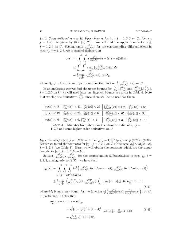
8.4.1. Computational results II. Upper bounds for |rj |, j = 1, 2, 3 on U . Let rj ,j = 1, 2, 3 be given by (8.21)–(8.23). We will find the upper bounds for |rj |,j = 1, 2, 3 on U . Setting again ∂2P

∂(ω,λ)αj for the corresponding differentiations ineach rj , j = 1, 2, 3, we in general deduce that

|rj(x)| = |∫ 1

0

∫ 1

0

s ∂2P∂(ω,λ)αj (a+ ts(x− a))dt ds|

≤∫ 1

0

∫ 1

0

s supx∈U

| ∂2P∂(ω,λ)αj (x)|dt ds

= 12 sup

x∈U| ∂2P∂(ω,λ)αj (x)| ≤ Qj ,

where Qj , j = 1, 2, 3 is an upper bound for the function 12 |

∂2P∂(ω,λ)αj (x)| on U .

In an analogous way we find the upper bounds for |∂rj

∂ω |, |∂rj

∂λ | and | ∂2rj

∂ω∂λ |, |∂2rj

∂λ2 |,j = 1, 2, 3 on U , we will need later on. Explicit bounds are given in Table 4. Notethat we skip the derivatives ∂2rj

∂ω2 since there will be no need for them.

|r1(x)| < 5 |∂r1∂ω (x)| < 43, |∂r1

∂λ (x)| < 25 | ∂2r1∂ω∂λ (x)| < 175, |∂

2r1∂λ2 (x)| < 65

|r2(x)| < 19 |∂r2∂ω (x)| < 25, |∂r2

∂λ (x)| < 6 | ∂2r2∂ω∂λ (x)| < 65, |∂

2r2∂λ2 (x)| < 33

|r3(x)| < 6 |∂r3∂ω (x)| < 6, |∂r3

∂λ (x)| < 4 | ∂2r3∂ω∂λ (x)| < 33, |∂

2r3∂λ2 (x)| < 16

Table 4. Estimates from above for the absolute value of rj , j =1, 2, 3 and some higher order derivatives on U

Upper bounds for |qj |, j = 1, 2, 3 on U . Let qj , j = 1, 2, 3 by given by (8.28) – (8.30).Earlier we found the estimates for |qj |, j = 1, 2, 3 on V of the type |qj | ≤Mj |x−a|,j = 1, 2, 3 (see Table 3). Here, we will obtain the constants which are the upperbounds for |qj |, j = 1, 2, 3 on U .

Setting ∂3P∂(ω,λ)αj ,

∂3P

∂(ω,λ)βjfor the corresponding differentiations in each qj , j =

1, 2, 3, analogously to (8.35), we have that

|qj(x)| = |∫ 1

0

∫ 1

0

∫ 1

0

ts2(

∂3P∂(ω,λ)αj (a+ tsσ(x− a)), ∂3P

∂(ω,λ)βj(a+ tsσ(x− a))

)× (x− a)T dσdt ds|

≤ 16 sup

x∈U|(

∂3P∂(ω,λ)αj (x), ∂3P

∂(ω,λ)βj(x)

)|max

U|x− a| ≤Mj max

U|x− a|,

(8.40)where Mj is an upper bound for the function 1

6 |(

∂3P∂(ω,λ)αj (x), ∂3P

∂(ω,λ)βj(x)

)| on U .

In particular, it holds that

maxU

|x− a| = |x− a|∣∣∂U

=√(

ω − 12π

)2 + (λ− 4)2∣∣(ω,λ)=(

12π− 2

180π,4−0.060)

=√

( 190π)2 + 0.0602,

(8.41)


andM1 = 44, M2 = 27, M3 = 11.

The explicit upper bounds are given in Table 5.

|q1(x)| < 3.1 |q2(x)| < 1.9 |q3(x)| < 0.8

Table 5. Estimates from above for |qj |, j = 1, 2, 3 on U

Lower bounds for F (x) = detB(x) and G(x) = b11(x) + 2√

detB(x) + b22(x) onU . Let us set

F (x) = detB(x),

G(x) = b11(x) + 2√

detB(x) + b22(x),(8.42)

bij , i, j = 1, 2 are given in (8.31)–(8.34) and find the lower bounds for F and Gon U . By construction of the ball WR(a) ⊃ U from Proposition 8.5 we know thatF ≥ 0 and G > 0 on WR(a). More precisely, for every x ∈ WR(a) (and hence forevery x ∈ U) it holds that

F (x) ≥ 1−√

24π |q2(x)| −

164 |q1(x)| −

132π2 |q1(x)||q3(x)|,

G(x) ≥ 2−√

24π |q2(x)| −

164 |q1(x)|.

Due to results of Table 5 we finally obtain that on U ,F (x) ≥ 0.730 · · · > 0.7,

G(x) ≥ 1.738 · · · > 1.7.(8.43)

Upper bounds for |bij |, i, j = 1, 2 on U . Let bij , i, j = 1, 2 be given by (8.24) –(8.27), namely,

b11(x) = 164r1(x)−

√2

8π r2(x),

b12(x) = 164r2(x)−

√2

8π r3(x),

b21(x) = −√

28π r1(x), b22(x) = −

√2

8π r2(x),

with rj , j = 1, 2, 3 as in (8.21)–(8.23).Using the results of Table 4 we will find the following upper bounds for the

absolute values of bij , i, j = 1, 2 and some higher order derivatives on U (see Table6).

|b11(x)| < 1.2 |∂b11∂ω (x)| < 2.1, |∂b11

∂λ (x)| < 0.8 |∂2b11

∂ω∂λ (x)| < 6.4, |∂2b11∂λ2 (x)| < 2.9

|b12(x)| < 0.7 |∂b12∂ω (x)| < 0.8, |∂b12

∂λ (x)| < 0.4 |∂2b12

∂ω∂λ (x)| < 2.9, |∂2b12∂λ2 (x)| < 1.5

|b21(x)| < 0.3 |∂b21∂ω (x)| < 2.5, |∂b21

∂λ (x)| < 1.5 |∂2b21

∂ω∂λ (x)| < 9.9, |∂2b21∂λ2 (x)| < 3.7

|b22(x)| < 1.1 |∂b22∂ω (x)| < 1.5, |∂b22

∂λ (x)| < 0.4 |∂2b22

∂ω∂λ (x)| < 3.7, |∂2b22∂λ2 (x)| < 1.9

Table 6. Estimates from above for the absolute value of bij , i, j =1, 2 and some higher order derivatives on U

Upper bounds for F (x) = detB(x) and G(x) = b11(x) + 2√

detB(x) + b22(x) onU . Recall that F and G are given by (8.42). They are positive functions on U


with lower bounds as in (8.43). Here we find their upper bounds together with theupper bounds for some higher order derivatives.

In particular, in order to obtain the estimates for F , |∂F∂ω |, |

∂F∂λ | and | ∂2F

∂ω∂λ |, |∂2F∂λ2 |

on U , we use the results of Table 6. The estimates found are presented in the firstrow of Table 7.

To find the estimates for |∂G∂ω |, |

∂G∂λ | and | ∂2G

∂ω∂λ |, |∂2G∂λ2 | we use

• the lower bound for Fon U , namely, F (x) > 0.7,• the results of Table 6 and• the results from the first row of Table 7.

E.g., for |∂G∂ω | we will have that on U

|∂G∂ω (x)| = |∂b11

∂ω (x) +∂F∂ω (x)√

F (x)+ ∂b22

∂ω (x)|

≤ supU|∂b11

∂ω (x)|+ supU |∂F∂ω (x)|

infU

√F (x)

+ supU|∂b22

∂ω (x)|

< 2.1 + 6.1√0.7

+ 1.5 ≈ 10.891 · · · < 11.

The other estimates on U for the derivatives of G listed above are obtained in ananalogous way and presented in Table 7.

F (x) < 1.53|∂F∂ω (x)| < 6.10,|∂F

∂λ (x)| < 2.53| ∂2F∂ω∂λ (x)| < 23.52,|∂

2F∂λ2 (x)| < 10.35

− |∂G∂ω (x)| < 11,|∂G

∂λ (x)| < 4.3| ∂2G∂ω∂λ (x)| < 51.4,|∂

2G∂λ2 (x)| < 22.7

Table 7. Estimates from above for F and G on U

Upper bounds for |cij |, i, j = 1, 2 on U . Let cij , i, j = 1, 2 be given by given by(8.15). It is convenient for further computations to set

cij(x) = bij(x)+A√

F (x)√G(x)

, (8.44)

where F and G are as in (8.42) and

A =

1 if (i, j) = (1, 1), (2, 2),0 if (i, j) = (1, 2), (2, 1).

To obtain the estimates for |∂cij

∂ω |, |∂cij

∂λ | and | ∂2cij

∂ω∂λ |, |∂2cij

∂λ2 |, i, j = 1, 2 on U we use• the lower bound for F and G on U , defined by formula (8.43),• the results of Table 6 and• the results of Table 7.

E.g., the estimate for |∂cij

∂λ | on U is found in the following way:

|∂cij

∂λ (x)| =∣∣ ∂bij

∂λ (x)√G(x)

+ 12A

∂F∂λ (x)√

G(x)√

F (x)− 1

2

∂G∂λ (x)

G3/2(x)

(bij(x) +A

√F (x)

) ∣∣≤

∣∣ supU |∂bij

∂λ (x)|

infU

√G(x)

+ 12A

supU |∂F∂λ (x)|

infU

“√G(x)

√F (x)

”


+ 12

supU |∂G∂λ (x)|

infU G3/2(x)

(supU|bij(x)|+A sup

U

√F (x)

) ∣∣.The other estimates on U for the derivatives of cij , i, j = 1, 2 listed are obtained inan analogous way and listed in Table 8 below.

|∂c11∂λ (x)| < 4.2

|∂2c11

∂ω∂λ (x)| < 99.4|∂

2c11∂λ2 (x)| < 35

|∂c12∂ω (x)| < 2.4

|∂c12∂λ (x)| < 1

|∂2c12

∂ω∂λ (x)| < 18.7|∂

2c12∂λ2 (x)| < 8.1

|∂c21∂λ (x)| < 1.5

|∂2c21

∂ω∂λ (x)| < 20.1|∂

2c21∂λ2 (x)| < 8.4

|∂c22∂ω (x)| < 9.8

|∂c22∂λ (x)| < 3.8

|∂2c22

∂ω∂λ (x)| < 94.4|∂

2c22∂λ2 (x)| < 38.7

Table 8. Estimates from above for the absolute value of somehigher order derivatives of cij , i, j = 1, 2 on U

Upper bounds for |hi|, i = 1, 2 on U . Let hi, i = 1, 2 be given by formulas (8.13),(8.14). First we compute the following derivatives of hi, i = 1, 2 we will need below:

∂h1∂λ (x) = c12(x) +

(∂c11∂λ (x), ∂c12

∂λ (x))(x− a)T

, (8.45)

∂2h1∂ω∂λ (x) = ∂c12

∂ω (x) + ∂c11∂λ (x) +

(∂2c11∂ω∂λ (x), ∂2c12

∂ω∂λ (x))

(x− a)T, (8.46)

∂2h1∂λ2 (x) = 2∂c12

∂λ (x) +(

∂2c11∂λ2 (x), ∂2c12

∂λ2 (x))

(x− a)T, (8.47)

∂h2∂λ (x) = c22(x) +

(∂c21∂λ (x), ∂c22

∂λ (x))(x− a)T

, (8.48)

∂2h2∂ω∂λ (x) = ∂c22

∂ω (x) + ∂c21∂λ (x) +

(∂2c21∂ω∂λ (x), ∂2c22

∂ω∂λ (x))

(x− a)T, (8.49)

∂2h2∂λ2 (x) = 2∂c22

∂λ (x) +(

∂2c21∂λ2 (x), ∂2c22

∂λ2 (x))

(x− a)T, (8.50)

where cij , i, j = 1, 2 are as in (8.44) and a =(

12π, 4

).

Using the results of Table 8 we find the estimates for | ∂2hi

∂ω∂λ |, |∂2hi

∂λ2 |, i = 1, 2 onU . E.g., for | ∂2h1

∂ω∂λ | it holds that on U :

| ∂2h1∂ω∂λ (x)| = |∂c12

∂ω (x) + ∂c11∂λ (x) +

(∂2c11∂ω∂λ (x), ∂2c12

∂ω∂λ (x))

(x− a)T |

≤ supU|∂c12

∂ω (x)|+ supU|∂c11

∂λ (x)|

+ supU|(

∂2c11∂ω∂λ (x), ∂2c12

∂ω∂λ (x))|max

U|x− a| < . . .

for maxU |x− a| see formula (8.41) and then

· · · < 2.4 + 4.2 +√

99.42 + 18.72

√(190π

)2 + 0.0602 ≈ 13.621 · · · < 13.7.

Analogously, the other estimates on U are obtained (see Table 9).


| ∂2h1∂ω∂λ (x)| < 13.7 | ∂2h2

∂ω∂λ (x)| < 18

|∂2h1

∂λ2 (x)| < 4.5 |∂2h2

∂λ2 (x)| < 10.4

Table 9. Estimates from above for the absolute value of somehigher order derivatives of hi, i = 1, 2 on U

8.4.2. Strict positivity of the functions ∂h2∂λ (ω, λ) and 16

√2∂h1

∂λ (ω, λ) + π ∂h2∂λ (ω, λ)

on U . Let us fix the notations which are common for two lemmas.

Notation 8.7. Let U be as in (8.37), namely,

U :=(ω, λ) :

[88180π,

92180π

]× [3.940, 4.060]

.

By (ωi, λj) i=0,...,nj=0,...,m

we mean a discretization of U which is defined as follows

ωi = 88180π + i∆ω, λj = 3.94 + j∆λ,

with

∆ω =4

180π

n , ∆λ = 0.12m .

Then we deduce the following two results.

Lemma 8.8. It holds that∂h2

∂λ(ω, λ) > 0 on U. (8.51)

Proof. Fix n = m = 2 and consider the discretization (ωi, λj)i,j of U given byNotation 8.7. By straightforward computations it holds that

∂h2∂λ (ωi, λj) > 0, (8.52)

for all i = 0, . . . , 2, j = 0, . . . , 2 and, moreover,

min(ωi,λj)∈U

∂h2∂λ (ωi, λj) = ∂h2

∂λ (ω0, λ0) ≈ 0.952 . . . . (8.53)

Next to this, we compute

a1 = max∆ω,∆λ

= max

4180π

n , 0.12m

= 0.12

2 = 0.060,

and, by taking into account the results of Table 9 and (8.53), we also find

a2 =√

2min(ωi,λj)∈U

∂h2∂λ (ωi, λj)

supU |(

∂2h2∂ω∂λ (ω, λ), ∂2h2

∂λ2 (ω, λ))|≈ 0.065 . . . .

Since a1 < a2, by Lemma 8.1 we conclude that the constructed discretization(ωi, λj)i=0,...,2

j=0,...,2of U to be appropriate in the sense that condition (8.52) yields a

strict positivity of ∂h2∂λ (ω, λ) on U .

Lemma 8.9. Let U be as in (8.37). It holds that

16√

2∂h1

∂λ(ω, λ) + π

∂h2

∂λ(ω, λ) > 0 on U. (8.54)


Proof. Fix n = 7, m = 12 and consider the discretization (ωi, λj)i,j of U givenby Notation 8.7. By straightforward computations it holds that

16√

2∂h1∂λ (ωi, λj) + π ∂h2

∂λ (ωi, λj) > 0, (8.55)


min(ωi,λj)∈U

(16√

2∂h1∂λ (ωi, λj) + π ∂h2

∂λ (ωi, λj))

= 16√

2∂h1∂λ (ω0, λ0) + π ∂h2

∂λ (ω0, λ0) ≈ 2.936 . . . .(8.56)


b1 = max∆ω,∆λ

= max

4180π

n , 0.12m

= 0.12

12 = 0.010,

and, by taking into account the results of Table 9 and (8.56), we also find

b2 =√

2min(ωi,λj)∈U

(16√

2∂h1∂λ (ωi, λj) + π ∂h2

∂λ (ωi, λj))

supU |(16√

2 ∂2h1∂ω∂λ (ω, λ) + π ∂2h2

∂ω∂λ (ω, λ), 16√

2∂2h1∂λ2 (ω, λ) + π ∂2h2

∂λ2 (ω, λ))|

≈ 0.011 . . . .

Since b1 < b2, by Lemma 8.1 we conclude that the constructed discretization(ωi, λj)i,j of U to be appropriate in the sense that condition (8.55) yields a strictpositivity of 16

√2∂h1

∂λ (ω, λ) + π ∂h2∂λ (ω, λ) on U .

8.5. On P (ω, λ) = 0 in V away from a = (12π, 4). Recall here function P defined

on V =(ω, λ) : [ 70

180π,110180π]× [2.900, 5.100]

:

P (ω, λ) =(1−

√2

2 sin(2ω))λ

+(1 +

√2

2 sin(2ω))λ

+(

12 + 1

2 cos2(2ω)) 1

2 λ[2 cos

(λ

(arctan

(√2

2 tan(2ω))

+ π))

− 4 cos(λ arctan

(tan2(ω)

)) ].

(8.57)

8.5.1. Set of Claims I. In a set of claims below we describe some properties of thefirst derivatives ∂P

∂ω and ∂P∂λ on V away from the point a =

(12π, 4

)which are used

in Lemma 4.11.

Claim 8.10. Let H1 ⊂ V be H1 =(ω, λ) :

[84180π,

90180π

]× [4.030, 4.970]

. It holds

that ∂P∂ω (ω, λ) < 0 on H1.

Proof. First we find the following estimates:

|∂2P

∂ω2(ω, λ)| < 162, | ∂2P

∂ω∂λ (ω, λ)| < 45 on H1. (8.58)

Then we fix n = 14, m = 120 and consider the discretization (ωi, λj)i,j of H1

such thatωi = 84

180π + i∆ω, λj = 4.030 + j∆λ,with

∆ω =6

180π

n , ∆λ = 0.94m .

By straightforward computations it holds that

−∂P∂ω (ωi, λj) > 0, (8.59)



min(ωi,λj)∈H1

(−∂P

∂ω (ωi, λj))

= −∂P∂ω (ω9, λ0) ≈ 1.022 . . . . (8.60)


c1 = max ∆ω,∆λ = max 6

180π

n , 0.94m

= 0.94

120 ≈ 0.00783 . . . ,

and, by taking into account (8.58) and (8.60), we also find

c2 =√

2min(ωi,λj)∈H1

(−∂P

∂ω (ωi, λj))

supH1

∣∣(∂2P∂ω2 (ω, λ), ∂2P

∂ω∂λ (ω, λ))∣∣ ≈ 0.00860 . . . .

Since c1 < c2, by Lemma 8.1 we conclude that the constructed discretization(ωi, λj) i=0,...,14

j=0,...,120of H1 to be appropriate in the sense that condition (8.59) yields

a strict positivity of −∂P∂ω (ω, λ) on H1, or, in other words, ∂P

∂ω (ω, λ) < 0 on H1.


[87180π,

101180π

]× [4.750, 5.100]

. It holds

that ∂P∂λ (ω, λ) > 0 on H2.


| ∂2P∂ω∂λ (ω, λ)| < 48, |∂

2P∂λ2 (ω, λ)| < 25 on H2. (8.61)

Then we fix n = 40, m = 55 and consider the discretization (ωi, λj)i,j , i =0, . . . , 40, j = 0, . . . , 55 of H2 such that

ωi = 87180π + i∆ω, λj = 4.750 + j∆λ,

with

∆ω =14180π

n , ∆λ = 0.35m .

By straightforward computations it holds that∂P∂λ (ωi, λj) > 0, (8.62)


min(ωi,λj)∈H2

∂P∂λ (ωi, λj) = ∂P

∂λ (ω0, λ0) ≈ 0.245 . . . . (8.63)


c1 = max ∆ω,∆λ = max 14

180π

n , 0.35m

= 0.35

55 ≈ 0.00636 . . . ,


c2 =√

2min(ωi,λj)∈H2

∂P∂λ (ωi, λj)

supH2

∣∣( ∂2P∂ω∂λ (ω, λ), ∂2P

∂λ2 (ω, λ))∣∣ ≈ 0.00641 . . . .

Since c1 < c2, by Lemma 8.1 we conclude that the constructed discretization(ωi, λj)i=0,...,40


a strict positivity of ∂P∂λ (ω, λ) on H2.


[100180π,

108180π

]× [4.000, 4.850]

. It holds

that ∂P∂ω (ω, λ) > 0 on H3.



|∂2P

∂ω2(ω, λ)| < 166, | ∂2P

∂ω∂λ (ω, λ)| < 37 on H3. (8.64)

Then we fix n = 10, m = 60 and consider the discretization (ωi, λj)i,j of H3 suchthat

ωi = 100180π + i∆ω, λj = 4.000 + j∆λ,

with

∆ω =8

180π

n , ∆λ = 0.85m .

By straightforward computations it holds that∂P∂ω (ωi, λj) > 0, (8.65)


min(ωi,λj)∈H3

∂P∂ω (ωi, λj) = ∂P

∂ω (ω0, λ11) ≈ 1.885 . . . . (8.66)



180π

n , 0.85m

= 0.85

60 ≈ 0.0142 . . . ,


c2 =√

2min(ωi,λj)∈H3

∂P∂ω (ωi, λj)

supH3

∣∣(∂2P∂ω2 (ω, λ), ∂2P

∂ω∂λ (ω, λ))∣∣ ≈ 0.0157 . . . .



a strict positivity of ∂P∂ω (ω, λ) on H3.

Claim 8.13. Let H4 ⊂ V be H4 = (ω, λ) : [ 91180π,

102180π]× [3.950, 4.100]. It holds

that ∂P∂λ (ω, λ) < 0 on H4.


| ∂2P∂ω∂λ (ω, λ)| < 38, |∂

2P∂λ2 (ω, λ)| < 11 on H4. (8.67)


ωi = 91180π + i∆ω, λj = 3.950 + j∆λ,

with

∆ω =11180π

n , ∆λ = 0.15m .


−∂P∂λ (ωi, λj) > 0, (8.68)


min(ωi,λj)∈H4

(−∂P

∂λ (ωi, λj))

= −∂P∂λ (ω0, λ0) ≈ 0.118 . . . . (8.69)


c1 = max ∆ω,∆λ = max 11

180π

n , 0.15m

= 0.15

36 = 0.00416 . . . ,



c2 =√

2min(ωi,λj)∈H4

(−∂P

∂λ (ωi, λj))

supH4

∣∣( ∂2P∂ω∂λ (ω, λ), ∂2P

∂λ2 (ω, λ))∣∣ ≈ 0.00423 . . . .



a strict positivity of −∂P∂λ (ω, λ) on H4, or, in other words ∂P

∂λ (ω, λ) < 0 on H4.


[90180π,

96180π

]× [3.030, 3.970]

. It holds

that ∂P∂ω (ω, λ) > 0 on H5.


|∂2P

∂ω2(ω, λ)| < 105, | ∂2P

∂ω∂λ (ω, λ)| < 37 on H5. (8.70)


ωi = 90180π + i∆ω, λj = 3.030 + j∆λ,

with

∆ω =6

180π

n , ∆λ = 0.94m .

By straightforward computations it holds that∂P∂ω (ωi, λj) > 0, (8.71)


min(ωi,λj)∈H5

∂P∂ω (ωi, λj) = ∂P

∂ω (ω0, λ0) ≈ 0.807 . . . . (8.72)



180π

n , 0.94m

= 0.94

94 ≈ 0.0100,


c2 =√

2min(ωi,λj)∈H5

∂P∂ω (ωi, λj)

supH5

∣∣(∂2P∂ω2 (ω, λ), ∂2P

∂ω∂λ (ω, λ))∣∣ ≈ 0.0102 . . . .



a strict positivity of ∂P∂ω (ω, λ) on H5.


[79180π,

94180π

]× [2.900, 3.230]

.

It holds that ∂P∂λ (ω, λ) < 0 on H6.


| ∂2P∂ω∂λ (ω, λ)| < 33, |∂

2P∂λ2 (ω, λ)| < 21 on H6. (8.73)


ωi = 79180π + i∆ω, λj = 2.900 + j∆λ,


with

∆ω =15180π

n , ∆λ = 0.33m .


−∂P∂λ (ωi, λj) > 0, (8.74)


min(ωi,λj)∈H6

(−∂P

∂λ (ωi, λj))

= −∂P∂λ (ω33, λ41) ≈ 0.227 . . . . (8.75)


c1 = max ∆ω,∆λ = max 15

180π

n , 0.33m

= 0.33

41 = 0.00805 . . . ,


c2 =√

2min(ωi,λj)∈H6

(−∂P

∂λ (ωi, λj))

supH6

∣∣( ∂2P∂ω∂λ (ω, λ), ∂2P

∂λ2 (ω, λ))∣∣ ≈ 0.00820 . . . .



a strict positivity of −∂P∂λ (ω, λ) on H6, or, in other words ∂P

∂λ (ω, λ) < 0 on H6.


[72180π,

80180π

]× [3.150, 4.000]

. It holds

that ∂P∂ω (ω, λ) < 0 on H7.


|∂2P

∂ω2(ω, λ)| < 115, | ∂2P

∂ω∂λ (ω, λ)| < 21 on H7. (8.76)

Then we fix n = 5, m = 30 and consider the discretization (ωi, λj)i,j , i = 0, . . . , 5,j = 0, . . . , 30 of H7 such that

ωi = 72180π + i∆ω, λj = 3.150 + j∆λ,

with

∆ω =8

180π

n , ∆λ = 0.85m .


−∂P∂ω (ωi, λj) > 0, (8.77)


min(ωi,λj)∈H7

(−∂P

∂ω (ωi, λj))

= −∂P∂ω (ω5, λ27) ≈ 2.663 . . . . (8.78)



180π

n , 0.85m

= 0.85

30 ≈ 0.0283 . . . ,


c2 =√

2min(ωi,λj)∈H7

(−∂P

∂ω (ωi, λj))

supH7

∣∣(∂2P∂ω2 (ω, λ), ∂2P

∂ω∂λ (ω, λ))∣∣ ≈ 0.0322 . . . .

Since c1 < c2, by Lemma 8.1 we conclude that the constructed discretization(ωi, λj) i=0,...,5


a strict positivity of −∂P∂ω (ω, λ) on H7, or, in other words, ∂P

∂ω (ω, λ) < 0 on H7.



[78180π,

89180π

]× [3.900, 4.050]

. It holds

that ∂P∂λ (ω, λ) > 0 on H8.


| ∂2P∂ω∂λ (ω, λ)| < 36, |∂

2P∂λ2 (ω, λ)| < 10 on H8. (8.79)


ωi = 78180π + i∆ω, λj = 3.900 + j∆λ,

with

∆ω =11180π

n , ∆λ = 0.15m .

By straightforward computations it holds that∂P∂λ (ωi, λj) > 0, (8.80)


min(ωi,λj)∈H8

∂P∂λ (ωi, λj) = ∂P

∂λ (ω40, λ30) ≈ 0.134 . . . . (8.81)


c1 = max ∆ω,∆λ = max 11

180π

n , 0.15m

= 0.15

30 = 0.00500,


c2 =√

2min(ωi,λj)∈H8

∂P∂λ (ωi, λj)

supH8sup

∣∣( ∂2P∂ω∂λ (ω, λ), ∂2P

∂λ2 (ω, λ))∣∣ ≈ 0.00508 . . . .



a strict positivity of ∂P∂λ (ω, λ) on H8.

8.5.2. Set of Claims II. Let H0 ⊂ V be as follows

H0 =(ω, λ) :

[84180π,

94180π

]× [2.960, 3.060]

.

Consider a function G : H0 → R given by

G(ω, λ) = −∂2P∂ω2 (ω, λ)

[∂P∂λ (ω, λ)

]−1+ 2 ∂2P

∂ω∂λ (ω, λ)∂P∂ω (ω, λ)

[∂P∂λ (ω, λ)

]−2

− ∂2P∂λ2 (ω, λ)

[∂P∂ω (ω, λ)

]2 [∂P∂λ (ω, λ)

]−3,

where P is as in (8.57).

Claim 8.18. It holds that G(ω, λ) > 0 on H0.


|∂G∂ω (ω, λ)| < 25000, |∂G

∂λ (ω, λ)| < 14000 on H0. (8.82)


ωi = 84180π + i∆ω, λj = 2.960 + j∆λ,

with

∆ω =10180π

n , ∆λ = 0.1m .



G(ωi, λj) > 0, (8.83)


min(ωi,λj)∈H0

G(ωi, λj) = G(ω0, λ0) ≈ 8.380 . . . . (8.84)


c1 = max ∆ω,∆λ = max 10

180π

n , 0.1m

= 0.1

300 ≈ 0.000(3),


c2 =√

2min(ωi,λj)∈H0 G(ωi, λj)

supH0

∣∣(∂G∂ω (ω, λ), ∂G

∂λ (ω, λ))∣∣ ≈ 0.000414 . . . .

Since c1 < c2, by Lemma 8.1 we conclude that the constructed discretization(ωi, λj)i,j of H0 to be appropriate in the sense that condition (8.83) yields astrict positivity of G(ω, λ) on H0.

Let H? ⊂ V be as follows

H? =(ω, λ) :

[93.5180 π,

95.5180 π

]× [3.030, 3.600]

.

Consider a function F : H? → R given by

F (ω, λ) = −∂2P∂λ2 (ω, λ)

[∂P∂ω (ω, λ)

]−1+ 2 ∂2P

∂ω∂λ (ω, λ)∂P∂λ (ω, λ)

[∂P∂ω (ω, λ)

]−2

− ∂2P∂ω2 (ω, λ)

[∂P∂λ (ω, λ)

]2 [∂P∂ω (ω, λ)

]−3,

where P is as in (8.57).

Claim 8.19. It holds that F (ω, λ) < 0 on H?.


|∂F∂ω (ω, λ)| < 180, |∂F

∂λ (ω, λ)| < 80 on H?. (8.85)

Then we fix n = 70, m = 1100 and consider the discretization (ωi, λj)i,j , i =0, . . . , 70, j = 0, . . . , 1100 of H? such that

ωi = 93.5180 π + i∆ω, λj = 3.030 + j∆λ,

with

∆ω =2

180π

n , ∆λ = 0.57m .


−F (ωi, λj) > 0, (8.86)


min(ωi,λj)∈H?

(−F (ωi, λj)) = −F (ω70, λ1100) ≈ 0.0773 . . . . (8.87)



180π

n , 0.57m

= 0.57

1100 = 0.000518 . . . ,


c2 =√

2min(ωi,λj)∈H?

(−F (ωi, λj))

supH?

∣∣(∂F∂ω (ω, λ), ∂F

∂λ (ω, λ))∣∣ ≈ 0.000555 . . . .


Since c1 < c2, by Lemma 8.1 we conclude that the constructed discretization(ωi, λj)i,j of H? to be appropriate in the sense that condition (8.74) yields astrict positivity of −F (ω, λ) on H?, or, in other words F (ω, λ) < 0 on H?.

9. Explicit formulas to the homogeneous problem in the cone whenω ∈

12π, π,

32π, 2π

Here we give the explicit solutions to the homogeneous problem (4.1) in Kω when

ω ∈

12π, π,

32π, 2π

.

9.1. Case ω = 12π. The eigenvalues λ in this case are determined by the charac-

teristic equation (see subsection 4.1):

2 + 2 cos(πλ)− 4 cos(

12πλ

)= 0, λ /∈ 0,±1 .

The set of positive solutions of the above equation reads as:

λj∞j=1 = λ3j−2, λ3j−1, λ3j∞j=1 = −1 + 4j, 4j, 1 + 4j∞j=1 .

Here every values λ3j−2, λ3j has algebraic and geometric multiplicity 1, while λ3j−1

has algebraic and geometric multiplicity 2.

j λj κ(j) u(j)q = rλj+1Φ

(j)q (θ)

1 3 1 x2y2

2-3 4 2

(x3y2

x2y3

4 5 1 x3y3

5 7 1 x6y2 − x2y6

6-7 8 2

(x7y2 − 7

3x3y6

x2y7 − 73x6y

8 9 1 x7y3 − x3y7

9 11 1 x10y2 − 14x6y6 + x2y10

10-11 12 2

(x11y2 − 22x7y6 + 11

3x3y10

x2y11 − 22x6y7 + 113

x10y3

12 13 1 x11y3 − 667

x7y7 + x3y11

etc.

Table 10. The first three groups of solutions u(j)q , q = 0, . . . , κ(j)−

1 of problem (4.1) in Kω of measure ω = 12π.

In the table above we see that the functions that solve the homogeneous problem(4.1) in Kω of measure ω = 1

2π are given by polynomials in x and y, which makesa difference to the case when the operator of the problem is the bilaplacian ∆2.

9.2. Case ω = π. The eigenvalues λ in this case are determined by the character-istic equation (see subsection 4.1):

sin2(πλ) = 0, λ 6= ±1,


plus the values λ = ±1, which are determined by the conditions P−1(π) = P1(π) =0. Hence, the set of positive solutions reads as

λj∞j=1 = j,

where λ1 = 1 has algebraic and geometric multiplicity 1, while λj for j ≥ 2 hasalgebraic and geometric multiplicity 2.

j λj κ(j) u(j)q = rλj+1Φ

(j)q (θ)

1 1 1 y2

2− 3 2 2xy2

y3

4− 5 3 2x2y2

xy3

6− 7 4 2x3y2

x2y3

etc.

Table 11. Some first solutions u(j)q , q = 0, . . . , κ(j)−1 of problem

(4.1) in Kω of measure ω = π.

Here, when the opening angle ω of Kω is π, as well as in the case ω = 12π, the

solutions (4.1) in Kω are given by polynomials in x and y. We can not achieve thiswhen the operator L of the problem is the bilaplacian ∆2.

9.3. Case ω = 32π. The characteristic equation P

(32π, λ

)= 0, λ 6= ±1, where P is

given in subsection 4.1, can be factorized and the eigenvalues λ are determined bythe system:

cos(

12πλ

)= 0, λ 6= ±1,

cos(

12πλ

)= 1, λ 6= ±1,

cos4(

12πλ

)+ cos3

(12πλ

)− 1

2 cos2(

12πλ

)− 1

2 cos(

12πλ

)+ 1

16 = 0, λ 6= ±1.

The solutions with positive real part of the system above read, respectively,

λn1∞n1=1 = 1 + 2n1∞n1=1 , λn2

∞n2=1 = 4n2∞n2=1 ,

λn3∞n3=1 = −1 + 2n3 + (−1)n3 (1− µ1)

∞n3=1 ,

λn4∞n4=1 = −1 + 2n4 + (−1)n4 (1− µ2)

∞n4=1 ,

λn5∞n5=1 =

−1 + 2n5 + (−1)n5+1 (1− γ1)± iγ2

∞

n5=1,

where µ1, µ2 are the first two positive solutions of the equation

s4 + s3 − 12s

2 − 12s+ 1

16 = 0, (9.1)

with s = cos(

12πµ

), while (γ1, γ2) is the first positive solution of (9.1) with s =

− cos(

12πγ1

)cosh

(12πγ2

)+i sin

(12πγ1

)sinh

(12πγ2

). The numerical approximations

(up to three digits) are the following: µ1 ≈ 0.536 . . . , µ2 ≈ 0.926 . . . and γ1 ≈0.345 . . . , γ2 ≈ 0.179 . . . .


Note also that every λn2 = 4n2, n2 = 1, 2.3, . . . has algebraic and geometricmultiplicity 2, while every λnk

, for each k = 1, 3, 4, 5 has algebraic and geometricmultiplicity 1. The set λj∞j=1 is the combination of the found sets above.

j λj κ(j) Φ(j)q (θ) u

(j)q = rλj+1Φ

(j)q (θ)

1,2,3-4,5-6 ≈ 0.536 . . . ,≈ 0.926 . . . ,≈ 1.655 . . .± i0.179 . . . ,≈ 2.345 . . .± i0.179 . . .

7 3 1 sin2(θ) cos2(θ) x2y2

8, 9 ≈ 3.074 . . . ,≈ 3.464 . . .

10-11 4 2

(sin2(θ) cos3(θ)

cos2(θ) sin3(θ)

(x3y2

x2y3

12, 13 ≈ 4.536 . . . ,≈ 4.926 . . . ,

14 5 1 sin3(θ) cos3(θ) x3y3

15-16,17-18 ≈ 5.655 . . .± i0.179 . . . ,≈ 6.345 . . .± i0.179 . . . ,

19 7 1 sin2(θ) cos2(θ)`cos4(θ)− sin4(θ)

´x6y2 − x2y6

20, 21 ≈ 7.074 . . . ,≈ 7.464 . . .

22− 23 8 2

(sin2(θ) cos3(θ)

`cos4(θ)− 7

3sin4(θ)

´cos2(θ) sin3(θ)

`sin4(θ)− 7

3cos4(θ)

´ (x7y2 − 7

3x3y6

x2y7 − 73x6y

etc.

Table 12. The first solutions (λj ,Φ(j)q ), q = 0, . . . , κ(j) − 1 of

(4.4) and the solutions u(j)q of (4.1) in Kω of measure ω = 3

2π. Thesituation without explicit formula is marked by “ . . . ”.

9.4. Case ω = 2π. The eigenvalues λ in this case are determined by the charac-teristic equation (see subsection 4.1):

cos4(πλ)− cos2(πλ) = 0, λ 6= ±1,

plus the values λ = ±1, which are determined by the conditions P−1(2π) =P1(2π) = 0. The positive solutions are given by the set

λj∞j=1 = 12j,

where λ2 = 1 has algebraic and geometric multiplicity 1, while λj for j = 1 andj ≥ 3 has algebraic and geometric multiplicity 2.

Acknowledgements. We thank the anonymous referee for his careful reading ofthe manuscript.

References

[1] Bernoulli, Jacob II., Essai theoretique sur les vibrations des plaques elastiques, rectangulaires

et libres. Nova Acta Academiae Scientiarum Imperialis Petropolitanae V (1789), p.197.[2] C. Bandle, M. Flucher, Table of inequalities in elliptic boundary value problems, Recent

progress in inequalities, Series: Math. Appl., vol. 430 (1996), 97–125.

[3] H. Blum, R. Rannacher, On the boundary value problem of the biharmonic operator ondomains with angular corners, Math. Meth. in the Appl. Sci. 2 (1980), 556–581.

[4] M. Costabel, M. Dauge, S. Nicaise, editors. Boundary value problems and integral equationsin nonsmooth domains, Lecture Notes in Ppure and Apllied Mathematics, Vol. 167. Marcel

Dekker, Inc., New York, 1995.


j λj κ(j) Φ(j)q (θ) u

(j)q = rλj+1Φ

(j)q (θ)

1 12

2 . . . . . .

2 1 1 sin2(θ) y2

3 32

2 . . . . . .

4-5 2 2

(sin2(θ) cos(θ)

sin3(θ)

xy2

y3

6 52

2 . . . . . .

7-8 3 2

(sin2(θ) cos2(θ)

sin3(θ) cos(θ)

x2y2

xy3

9 72

2 . . . . . .

10-11 4 2

(sin2(θ) cos3(θ)

sin3(θ) cos2(θ)

x3y2

x2y3

etc.

Table 13. Some first solutions (λj ,Φ(j)q ), q = 0, . . . , κ(j) − 1 of

(4.4) and the solutions u(j)q of (4.1) in Kω of measure ω = 2π. The

situation when the explicit formula unavailable is marked by “. . . ”.

[5] Ph. Clement, G. Sweers, Uniform anti-maximum principles, J.Differential Equations 164

(2000), 118–154.[6] B. Dacorogna, Introduction to the calculus of variations, Imperial College Press, London,

2004.[7] M. Dauge, Elliptic boundary value problems on corner domains; smoothness and asymptotics

of solutions, Springer, Berlin, 1988.

[8] P. Drabek, J. Milota, Methods of Nonlinear Analysis: Applications to Differential Equations,Birkhauser Verlag, Basel, 2007.

[9] L.C. Evans, Partial differential equations. Graduate Studies in Mathematics, 19. American

Mathematical Society, Providence, RI, 1998.[10] P. Grisvard, Singularities in boundary value problems, Springer-Verlag, Berlin, 1992.

[11] G. Kirchhoff, Uber das Gleichgewicht und die Bewegung einer elastischen Scheibe. J. reineangew. Math. 40 (1850), 51–88.

[12] V.A. Kondratiev, Boundary value problems for elliptic equations in domains with conical or

angular points, Trudy Moskov. Mat. Ob sc. 16 (1967), 209–292 (in Russian), English transl.:Trans. Moscow Math. Soc. 16 (1967), 227–313.

[13] V.A. Kozlov, V.G. Maz’ya, J. Rossmann, Elliptic Boundary Value Problems in Domains withPoint Singularities, Mathematical Surveys and Monographs, vol. 52, American MathematicalSociety, Providence, RI, 1997.

[14] V.A. Kozlov, V.G. Maz’ya, J. Rossmann, Spectral problems associated with corner singu-

larities of solutions to elliptic equations, Mathematical Surveys and Monographs, vol. 85,American Mathematical Society, Providence, RI, 2001.

[15] B. Kawohl, G. Sweers, On the differential equation uxxxx + uyyyy = f for an anisotropicstiff material, SIAM J. Math. Anal., Vol. 37, No. 6 (2006), 1828–1853.

[16] D. Leguillon, E. Sanchez-Palencia, Computation of singular solutions in elliptic problems andelasticity, Masson, Paris, 1987.

[17] J.-L. Lions, E. Magenes, Non-homogeneous boundary value problems and applications, Vol.

I, Springer-Verlag, Berlin, 1972.

[18] S.A. Nazarov, B.A. Plamenevsky, Elliptic problems in domains with piecewise smooth bound-aries, De Gruyter, Berlin, 1994.

[19] S.A. Nazarov, A. Slutskij, G. Sweers, Korn’s inequalities for a reinforced plate, submitted.


[20] S.A. Nazarov, G. Sweers, A hinged plate equation and iterated Dirichlet Laplace operator on

domains with concave corners, J. Differential Equations 233 (2007), 151–180.

[21] R.S. Palais, The Morse lemma for Banach spaces, Bull. Amer. Math. Soc. 75 (1969), 968–971.

Tymofiy GerasimovDIAM-EWI, Delft University of Technology, PO box 5031, 2600 GA Delft, The Nether-

lands

E-mail address: [email protected]

Guido Sweers

MI, Universitat zu Koln, D 50931 Cologne, GermanyE-mail address: [email protected]

Date post:	27-Aug-2018
Category:	Documents
Upload:	vokhanh
View:	215 times
Download:	0 times

REGULARITY FOR A CLAMPED GRID EQUATION … · Dirichlet problem with this special non-isotropic...

Documents