Research ArticleStudy of the Bullwhip Effect under Various ForecastingMethods in Electronics Supply Chain with Dual Retailersconsidering Market Share

Junhai Ma ,1 Jing Zhang,1 and Liqing Zhu 1,2

1College of Management and Economics, Tianjin University, Tianjin 300072, China2School of HUAXIN Software, Tianjin University of Technology, Tianjin 300384, China

Correspondence should be addressed to Liqing Zhu; Lqzhu20080818@126.Com

Received 13 April 2017; Accepted 17 July 2017; Published 8 January 2018

Academic Editor: Soheil Salahshour

Copyright © 2018 Junhai Ma et al. This is an open access article distributed under the Creative Commons Attribution License,which permits unrestricted use, distribution, and reproduction in any medium, provided the original work is properly cited.

We establish in this paper a new two-stage supply chain with onemanufacturer and two retailers which have a fixedmarket share inthe mature and stable market with specific reference to consumer electronics industry.This paper offers insights into how the threeforecasting methods affect the bullwhip effect considering the market share under the ARMA(1, 1) demand process and the order-up-to inventory policy. We also discuss the stability of the order with the theory of entropy. In particular, we derive the expressionsof bullwhip effect measure under theMMSE, MA, and ESmethods and compare them by numerical simulations. Results show thatthe MA is always better in contrast to the ES for reducing the bullwhip effect in our supply chain model. When moving averagecoefficient is lower than a certain value, the MMSE method is the best for reducing the bullwhip effect; otherwise, the MAmethodis the best. Moreover, the larger the market share of the retailer with a long lead time is, the greater the bullwhip effect is, no matterwhat the forecasting method is.

1. Introduction

There is a high-risk behavior occurring frequently in manycompanies’ marketing activities, which is called bullwhipeffect, first coined by Lee et al. [1, 2]. It affects operational costsand may lead to chaos in the system. Because of its impact onthe operation and management strategies of all the upstreamand downstream enterprises, it has become a focus in thesupply chainmanagement research. In this paper, we focus onthe consumer electronics supply chain management, whichis characterized by frequent channel competition. In theChinese consumer electronics offline retail market, GOMEand SUNING are two giant chain enterprises, which occupymore than 45% of the market share. Most of the consumerelectronics manufacturers sell products through these twohome appliance retail chain stores. The market demand fore-casting and replenishment strategies of the two retail giantswill undoubtedly affect order fluctuations and productionplan of the manufacturers. We assume that the demand isindependent because GOME is far apart from SUNING.

So, we use the ARMA(1, 1) demand process and aim toinvestigate the effect of three forecasting methods on thebullwhip effect considering the market share.

Bullwhip effect refers to a phenomenon where the ordervariability tends to be amplified in a supply chain from thedownstream member to its (immediate) upstream member.Forrester [3, 4] discovered bullwhip effect’s causes and pos-sible remediation by industrial dynamics and became thefirst scholar proving this phenomenon. This was the firstmilestone in the academic research of bullwhip effect. Then,many other researchers further proved the existence of thebullwhip effect. A well-known classic “beer game” experi-mented on by Sterman [5] is the second milestone whichhas been utilized in business schools for decades to illustratethe bullwhip effect. The third milestone, also very important,is the statistical research stage which was started by Leeet al. [1, 2]. He identified five main causes of the bullwhipeffect which are demand signal processing, supply shortage,nonzero lead time, price fluctuation, and order batching insupply chains. After that, more and more researchers studied

HindawiComplexityVolume 2018, Article ID 8539740, 19 pageshttps://doi.org/10.1155/2018/8539740

2 Complexity

the bullwhip effect by statistical methods. Based on the worksof Lee, different demand processes and forecasting methodswhich directly affected the inventory system of supply chainssignificantly are employed in a lot of papers.

Similar to Lee et al. [1, 2], many papers are published foran AR(1) demand model in a two-stage supply chain withone manufacturer and one retailer [6–10]. Chen et al. [6, 7]studied the difference of bullwhip effects under two fore-casting methods (MA and ES) in a simple, two-stage supplychain. Zhang [8] investigated the impact of three differentforecasting methods (MA, ES, and MMSE) on the bullwhipeffect under AR(1) demand process. Lee et al. [9] also mea-sured the benefit of information sharing on reducing thebullwhip effect using AR(1) process and a simple order-up-to inventory policy with the minimum mean square error(MMSE) forecasting technique. Likewise, Luong [10] used thesame demand model as Lee et al. [9] to measure the bullwhipeffect on the base stock policy for their inventory underthe MMSE forecasting technique. Furthermore, Luong andPhien [11] investigated AR(2) demand process and higherorder autoregressive models AR(𝑝) with the MMSE method.By calculating the bullwhip effect, these papers investigatedeffects of different parameters on the bullwhip effect, such asautoregressive coefficients and order lead time. In addition,Duc et al. [12] measured the impact of a third-party ware-house on the bullwhip effect and inventory cost under AR(1)process in a three-stage supply chain with one manufacturer,one third-party warehouse, and two retailers consideringmarket share.

A pure autoregressive process has been supposed by a fewacademics [1, 2, 6–12], and a puremoving average process hasalso been used by Graves [13]. However, we can get that thedemandmodel has both characteristics of them. Pindyck andRubinfeld [14] assumed the mixed autoregressive-movingaverage (ARMA) demand process which is more suitable forthemarket demand than AR(1) model.Then, the ARMApro-cess is frequently applied. Under the base stock policy, Disneyet al. [15] used ARMA(1, 1) demand pattern to measure thebullwhip effect by the ES forecasting method in a singlesupply chain echelon. Duc et al. [16] focused on the impact ofsome parameters on the bullwhip effect via an ARMA(1, 1)model by the MMSE method. Likewise, Feng and Ma [17]evaluated the difference of MA, ES, and MMSE forecastingmethods, with the ARMA(1, 1) model by using the dynamicsimulation. The ARMA(1, 1) demand model is applied in allthe above papers in a single supply chain with one manufac-turer and one retailer. But, as an extension, a new supply chainwith onemanufacturer and two retailerswhoboth employ theARMA(1, 1) demand process is made, and emphasis is put onthe competition between the two retailers analyzed [18, 19].This model also compared the impact of parameters on thebullwhip effect under various forecastingmethods.Moreover,Bandyopadhyay and Bhattacharya [20] primarily studied thevarious replenishment policies to derive expressions of BWEbased on the generalized ARMA(𝑝, 𝑞) demand process inorder to get the appropriate replenishment policy for theminimum BWE.

As a further expansion of the ARMA demand model,Gilbert [21] conducted a new Autoregressive Integrated

Moving Average (ARIMA) time-series model to present thecauses of the bullwhip effect and managerial insights aboutreducing the bullwhip effect in a multistage supply chainmodel. Dhahri and Chabchoub (2007) also used an ARIMAdemand pattern to alleviate the bullwhip effect in two aspectsof increase of the stock level and reduction of the servicegiven back to customers. Nagaraja et al. [22] measured thebullwhipmeasure for a two-stage supply chain with an order-up-to inventory policy and derived a general, stationarySARMA(𝑝, 𝑞) × (𝑃, 𝑄)𝑠 demand process.

Many scholars research the systematic problem combin-ing the entropy theory. By using the tool of entropy, Han etal. [23] built a duopoly game model and investigated how thetime delay influences the stability of the system. Ma and Si[24] researched a Bertrand duopoly game model with two-stage delay and discussed the stability of the economic sys-tem.

This paper derives the expressions of the bullwhip effectunder various forecastingmethods in a two-stagemature andstable supply chain with one manufacturer and two retailerswhich have a fixed market share. With the development ofinformation technology, all electronic manufacturers takestrategies to shorten the length of supply chain and takenew information technologies to speed up the logistics. Forinstance, Haier, one of the largest household electrical appli-ances manufacturers all over the world, has been benefitingfrom the application of ERP and BBP since the begin-ning of the 21st century. The information management sys-tem performs information synchronization and integration,improves the real-time and accuracy of the information, andspeeds up the response speed of the supply chain. Therefore,the flat supply chain is common in reality. Based on this,we assume that both retailers face an ARMA(1, 1) demandprocess and employ the order-up-to replenishment policy. Inthe current research, we analyze the impact of parameterson the BWE under the MMSE, MA, and ES forecastingmethods and compare the differences of the three methodson dampening the bullwhip effect.

This paper differs from the previous research in thefollowing. First, the ARMA(1, 1) demandmodel of two retail-ers with a certain market share which is not considered inprevious papers is established in a mature and stable productmarket. Second, this paper evaluates the impact of themarketshare on the bullwhip effect and compares three forecastingmethods in this two-stage supply chain.

The remaining part of this paper is organized as follows.In Section 2, we present the demand process with the marketshare in a new supply chain with one manufacturer andtwo retailers which both employ the order-up-to inventorypolicy. In Section 3, we derive the bullwhip effect measureunder MMSE, MA, and ES forecasting methods. Underdifferent forecasting methods, the behavior of the bullwhipeffect is investigated and the effects of parameters on thebullwhip effect are discussed in Section 4, and then wecompare the impact of the three forecasting methods onthe bullwhip effect by numerical simulations. Finally, a shortconclusion is stated for this paper in Section 5. Proofs of somepropositions in this paper are summarized in the Appen-dix.

Complexity 3

Retailer 2

Retailer 1

Supplier

qt

q1,t

q2,t

d1,t

d2,t

1 − dt

Customer

Figure 1: Two-stage supply chain model.

2. Supply Chain Model

The two-level supply chain model shown in Figure 1, consist-ing of one manufacturer with a distribution center and tworetailers in the same market, is common in the consumerelectronics industry. A hypothesis is that the supply chainis in a stable market. So, we assume that our two retailersare in a duopolistic competitive industry, who both havefixed share of the market of customer demand, 𝛼 and 1 − 𝛼,respectively. The two retailers both master the accuratemarket information and their customer demands, which areARMA(1, 1) processes, and place orders to the manufacturer,respectively. The manufacturer obtains the orders directlyfrom the retailers and arranges the delivery to the nearestdistribution center as soon as possible, and the retailers takethe products back immediately once what they ordered hasarrived. The new supply chain model is presented in thissection.

2.1.DemandProcess. Considerretailer 1 facinganARMA(1, 1)demand of the form

𝑑1,𝑡 = 𝛼𝛿 + 𝜙𝑑1,𝑡−1 + 𝛼𝜀𝑡 − 𝛼𝜃𝜀𝑡−1. (1)

Here, 𝑑1,𝑡 represents unit demand in the period 𝑡. 𝜙 is theautoregressive coefficient, and |𝜙| < 1. 𝜃 is the first-ordermoving average coefficient, where −1 < 𝜃 < 1. 𝜀𝑡 is therandom error of the customer demand, and 𝜀𝑡 is independentand identically distributed from a normal distribution withmean 0 and variance 𝜎2. 𝛼 is the market share of retailer 1.

Since the demand process is stationary, there is

𝐸 (𝑑1,𝑡) = 𝐸 (𝑑1,𝑡−1) = 𝐸 (𝑑1) ,Var (𝑑1,𝑡) = Var (𝑑1,𝑡−1) = Var (𝑑1) ,

∀𝑡.(2)

Hence, a stationary condition can be given as

𝐸 (𝑑1) = 𝛼𝛿1 − 𝜙 .Var (𝑑1) = 𝛼2 (1 + 𝜃2 − 2𝜙𝜃)

1 − 𝜙2 Var (𝜀𝑡) .(3)

Similarly, retailer 2 also has an ARMA(1, 1) demandmodel

𝑑2,𝑡 = (1 − 𝛼) 𝛿 + 𝜙𝑑2,𝑡−1 + (1 − 𝛼) 𝜀𝑡 − (1 − 𝛼) 𝜃𝜀𝑡−1. (4)

Here, 𝜙 and 𝜃 have the same property with retailer 1 accord-ingly. 1 − 𝛼 is the market share of retailer 2.

For retailer 2, we also assume

𝐸 (𝑑2,𝑡) = 𝐸 (𝑑2,𝑡−1) = 𝐸 (𝑑2) ,Var (𝑑2,𝑡) = Var (𝑑2,𝑡−1) = Var (𝑑2) ,

∀𝑡.(5)

So, we can have

𝐸 (𝑑2) = (1 − 𝛼) 𝛿1 − 𝜙 .Var (𝑑2) = (1 − 𝛼)2 (1 + 𝜃2 − 2𝜙𝜃)

1 − 𝜙2 Var (𝜀𝑡) .(6)

In our research, based on the demand models of tworetailers, the total customer demand 𝑑𝑡 also faces anARMA(1, 1), as follows:

𝑑𝑡 = 𝛿 + 𝜙𝑑𝑡−1 + 𝜀𝑡 − 𝜃𝜀𝑡−1. (7)

Then, we have

𝑑1,𝑡 = 𝛼𝑑𝑡,𝑑2,𝑡 = (1 − 𝛼) 𝑑𝑡. (8)

2.2. Inventory Policy. For supplying the demand, we assumethe order-up-to inventory policy during the replenishmentperiod, which is studied in the supply chain model by Chenet al. [6]. This paper assumes that two retailers both employa simple order-up-to inventory policy in which the order-up-to level is determined to achieve a desired service level.Retailer 1 places an ordered quantity 𝑞1,𝑡 to the manufacturerat the beginning of period 𝑡 to be delivered at the beginningof period 𝑡 + 𝐿1, where 𝐿1 is the fixed lead time for themanufacturer to fulfill an order of retailer 1. The orderquantity 𝑞1,𝑡 can be given as

𝑞1,𝑡 = 𝑆1,𝑡 − 𝑆1,𝑡−1 + 𝑑1,𝑡−1, (9)

where 𝑆1,𝑡 is the order-up-to inventory position at the begin-ning of period 𝑡 of retailer 1 after placing the order in period 𝑡.While the base stock policy [16] is employed, the order-up-tolevel 𝑆1,𝑡 can be determined by the sum of forecasted lead-time demand and the safety stock as

𝑆1,𝑡 = 𝐷𝐿11,𝑡 + 𝑧�̂�𝐿11,𝑡 , (10)

in which 𝐷𝐿11,𝑡 is the forecast for the lead-time demand ofretailer 1 which depends on the forecasting method and leadtime 𝐿1, �̂�𝐿11,𝑡 is the standard deviation of lead-time demandforecast error, and 𝑧 is the normal 𝑧 score determined basedon a desired service level (the optimal order-up-to level 𝑆𝑡can be implicitly determined from inventory holding costand shortage cost for backorders (Heyman and Sobel, 1984[8]); however, since it is usually not easy to estimate thesecosts accurately in practice, the approach of using the service

4 Complexity

levels is often employed when the order-up-to level is to bedetermined).

Similarly, for retailer 2, the order quantity 𝑞2,𝑡, which isplaced to the manufacturer in period 𝑡 to be delivered at thebeginning of period 𝑡 + 𝐿2, where 𝐿2 is the fixed lead time ofretailer 1, can be given as

𝑞2,𝑡 = 𝑆2,𝑡 − 𝑆2,𝑡−1 + 𝑑2,𝑡−1. (11)

The order-up-to level of retailer 2 at period 𝑡 is𝑆2,𝑡 = 𝐷𝐿12,𝑡 + 𝑧�̂�𝐿12,𝑡 . (12)

Equations (11)-(12) have the same meaning as (9)-(10).

2.3. Forecasting Method. In this paper, we assume that tworetailers both use the same forecasting method to forecastthe lead-time demand.Commonly, there are three forecastingtechniques, MA, ES, and MMSE, for demand forecast. Asmentioned above, they have been used in most similarresearches. Here, in our paper, according to the demandprocess, we choose appropriate forecasting methods.

In Section 3, the bullwhip effect will be measured, respec-tively, under the MMSE, MA, and ES forecasting methods.Those three forecasting methods will be introduced in thissection firstly.

2.3.1. TheMMSE Forecasting Method. In the minimummeansquare error (MMSE) forecasting method, the lead-timedemand forecast𝐷𝐿𝑡 is given as

𝐷𝐿𝑡 = 𝑑𝑡 + 𝑑𝑡+1 + ⋅ ⋅ ⋅ + 𝑑𝑡+𝐿−1 = 𝐿−1∑𝑖=0

𝑑𝑡+𝑖, (13)

where 𝑑𝑡 is the forecast of the demand in period 𝑡, which canbe determined as

𝑑𝑡+𝑖 = 𝐸 [𝑑𝑡+𝑖 | 𝑑𝑡−1, 𝑑𝑡−2, . . .] . (14)

Under the ARMA(1, 1) model, we can have the customerdemand in the period of 𝑡 + 𝑖 by the recursive iteration of 𝑑𝑡based on (7):

𝑑𝑡+𝑖 = 1 − 𝜙𝑖+11 − 𝜙 𝛿 + 𝜙𝑖+1𝑑𝑡−1 − 𝜃 𝑖∑𝑗=0

𝜙𝑗𝜀𝑡+𝑖−𝑗−1+ 𝑖∑𝑗=0

𝜙𝑗𝜀𝑡+𝑖−𝑗.(15)

Then, the forecasting of the demand 𝑑𝑡+𝑖 by the MMSEmethod is as follows:

𝑑𝑡+𝑖 = 1 − 𝜙𝑖+11 − 𝜙 𝛿 + 𝜙𝑖+1𝑑𝑡−1 − 𝜙𝑖𝜃𝜀𝑡−1. (16)

According to (13) and (16), the total forecasting demandfor future 𝐿-periods can be simplified as

𝐷𝐿𝑡 = 𝐿1 − 𝜙𝛿 −𝜙 (1 − 𝜙𝐿)(1 − 𝜙)2 𝛿 + 𝜙 (1 − 𝜙𝐿)

1 − 𝜙 𝑑𝑡−1− 𝜃 (1 − 𝜙𝐿)

1 − 𝜙 𝜀𝑡−1.(17)

2.3.2.TheMAForecastingMethod. Using themoving average(MA) forecasting method, we first have the 𝜏-period-aheaddemand forecast given by

𝑑𝑡+𝜏 = 𝑑𝑡 = 1𝑘𝑘∑𝑖=1

𝑑𝑡−𝑖, 𝜏 ≥ 1, (18)

in which 𝑘 is the span (number of date points) for the MAforecasting method. Then, the lead-time demand forecast isgiven as

𝐷𝐿𝑡 = 𝐿𝑘𝑘∑𝑖=1

𝑑𝑡−𝑖. (19)

2.3.3.The ES Forecasting Method. TheES forecasting methodis an adaptive algorithm in which one-period-ahead forecastis adjusted with a fraction of the forecasting error. Thedemand forecast with ES can be written as

𝑑𝑡 = 𝜆𝑑𝑡−1 + (1 − 𝜆) 𝑑𝑡−1, (20)

where 𝜆 denotes the fraction used in this process, also calledthe smoothing factor, and 0 < 𝜆 < 1.3. Measure of Bullwhip Effect consideringMarket Share

In this section, we derive the measure of the bullwhip effectin a supply chain with one manufacturer and two retailerswhich both have stable market share, under the MMSE, MA,and ES forecasting methods mentioned above, respectively.From an early start, the bullwhip effect is a phenomenon inwhich the variance of demand information is amplified whenmoving upstream in a supply chain. Thus, it is reasonableto measure the bullwhip effect by the ratio of the varianceof order quantities experienced by the manufacturer to theactual variance of demand quantities. This means has beenused in previous researches such as those of Chen et al. [6, 7]and Duc et al. [12], and it is adopted in our research aswell.

In our model, according to (7)-(8), the total demand ofretailers 𝑑𝑡 is distributed as the ARMA(1, 1) model. Take thevariance of 𝑑𝑡; we have

Var (𝑑𝑡) = (1 + 𝜃2 − 2𝜙𝜃)1 − 𝜙2 Var (𝜀𝑡) . (21)

Complexity 5

3.1. Measure of the Bullwhip Effect under the MMSE Forecast-ingMethod. As stated in Section 3.2, the order of retailer 1 𝑞1,𝑡can be given as

𝑞1,𝑡 = 𝑆1,𝑡 − 𝑆1,𝑡−1 + 𝑑1,𝑡−1= 𝐷𝐿11,𝑡 − 𝐷𝐿11,𝑡−1 + 𝑧 (�̂�𝐿11,𝑡 − �̂�𝐿11,𝑡−1) + 𝑑1,𝑡−1. (22)

According to (17), the forecasting of the lead-timedemand for retailer 1 is

𝐷𝐿11,𝑡 = 𝐿11 − 𝜙𝛼𝛿 −𝜙 (1 − 𝜙𝐿1)(1 − 𝜙)2 𝛼𝛿 + 𝜙 (1 − 𝜙𝐿1)

1 − 𝜙 𝑑1,𝑡−1

− 𝛼𝜃 (1 − 𝜙𝐿1)1 − 𝜙 𝜀𝑡−1.

(23)

And the variance of lead-time demand forecast error, �̂�𝐿11,𝑡 ,does not depend on 𝑡.

Thus, taking (23) into (22), 𝑞1,𝑡 can be determined as

𝑞1,𝑡 = 𝜙 (1 − 𝜙𝐿1)1 − 𝜙 𝑑1,𝑡−1 − 𝛼𝜃 (1 − 𝜙𝐿1)

1 − 𝜙 𝜀𝑡−1− (𝜙 (1 − 𝜙𝐿1)

1 − 𝜙 𝑑1,𝑡−2 − 𝛼𝜃 (1 − 𝜙𝐿1)1 − 𝜙 𝜀𝑡−2)

+ 𝑑1,𝑡−1= (𝜙𝐴1 + 1) 𝑑1,𝑡−1 − 𝜙𝐴1𝑑1,𝑡−2

− 𝛼𝜃𝐴1 (𝜀𝑡−1 − 𝜀𝑡−2) ,

(24)

where 𝐴1 = (1 − 𝜙𝐿1)/(1 − 𝜙).Since 𝑑1,𝑡 = 𝛼𝑑𝑡, 𝑞1,𝑡 can be rewritten as

𝑞1,𝑡 = (𝜙𝐴1 + 1) 𝛼𝑑𝑡−1 − 𝜙𝐴1𝛼𝑑𝑡−2− 𝛼𝜃𝐴1 (𝜀𝑡−1 − 𝜀𝑡−2) . (25)

Likewise, we also have �̂�𝐿22,𝑡 = �̂�𝐿22,𝑡−1, and based on (24)and 𝑑2,𝑡 = (1 − 𝛼)𝑑𝑡, the order of retailer 2 in period 𝑡 can bewritten as

𝑞2,𝑡 = (𝜙𝐴2 + 1) (1 − 𝛼) 𝑑𝑡−1 − 𝜙𝐴2 (1 − 𝛼) 𝑑𝑡−2− (1 − 𝛼) 𝜃𝐴2 (𝜀𝑡−1 − 𝜀𝑡−2) , (26)

where 𝐴2 = (1 − 𝜙𝐿2)/(1 − 𝜙).

In this way, the order quantity of both retailers under theMMSE forecasting method in the period of 𝑡 is

𝑞𝑡 = 𝑞1,𝑡 + 𝑞2,𝑡= (𝜙𝐴1 + 1) 𝛼𝑑𝑡−1 − 𝜙𝐴1𝛼𝑑𝑡−2

− 𝛼𝜃𝐴1 (𝜀𝑡−1 − 𝜀𝑡−2) + (𝜙𝐴2 + 1) (1 − 𝛼) 𝑑𝑡−1− 𝜙𝐴2 (1 − 𝛼) 𝑑𝑡−2 − (1 − 𝛼) 𝜃𝐴2 (𝜀𝑡−1 − 𝜀𝑡−2)

= (1 + 𝛼𝜙𝐴1 + (1 − 𝛼) 𝜙𝐴2) 𝑑𝑡−1− (𝛼𝜙𝐴1 + (1 − 𝛼) 𝜙𝐴2) 𝑑𝑡−2− (𝛼𝜃𝐴1 + (1 − 𝛼) 𝜃𝐴2) 𝜀𝑡−1+ (𝛼𝜃𝐴1 + (1 − 𝛼) 𝜃𝐴2) 𝜀𝑡−2.

(27)

Proposition 1. The variance of total order quantity of tworetailers under the MMSE forecasting method in the period of𝑡 can be determined as

Var (𝑞𝑡) = [(1 + 𝛼𝜙𝐴1 + (1 − 𝛼) 𝜙𝐴2)2 + (𝛼𝜙𝐴1+ (1 − 𝛼) 𝜙𝐴2)2 − 2 (1 + 𝛼𝜙𝐴1 + (1 − 𝛼) 𝜙𝐴2)⋅ (𝛼𝜙𝐴1 + (1 − 𝛼) 𝜙𝐴2) (𝜙 − 𝜃) (1 − 𝜙𝜃)1 + 𝜃2 − 2𝜙𝜃 + 2⋅ 1 − 𝜙21 + 𝜃2 − 2𝜙𝜃 ((𝛼𝜃𝐴1 + (1 − 𝛼) 𝜃𝐴2)2− (1 + 𝛼𝜙𝐴1 + (1 − 𝛼) 𝜙𝐴2) (𝛼𝜃𝐴1 + (1 − 𝛼) 𝜃𝐴2)+ (1 + 𝛼𝜙𝐴1 + (1 − 𝛼) 𝜙𝐴2) (𝛼𝜃𝐴1 + (1 − 𝛼) 𝜃𝐴2)⋅ (𝜙 − 𝜃) − (𝛼𝜙𝐴1 + (1 − 𝛼) 𝜙𝐴2)⋅ (𝛼𝜃𝐴1 + (1 − 𝛼) 𝜃𝐴2))]Var (𝑑𝑡) .

(28)

Proof. See Appendix A.

As the definition, the bullwhip effect in the supplychain with two retailers by the MMSE method, denoted byBWEmmse, is derived as

BWEmmse = Var (𝑞𝑡)Var (𝑑𝑡) = (1 + 𝛼𝜙𝐴1 + (1 − 𝛼) 𝜙𝐴2)2

+ (𝛼𝜙𝐴1 + (1 − 𝛼) 𝜙𝐴2)2 − 2 (1 + 𝛼𝜙𝐴1 + (1 − 𝛼)⋅ 𝜙𝐴2) (𝛼𝜙𝐴1 + (1 − 𝛼) 𝜙𝐴2) (𝜙 − 𝜃) (1 − 𝜙𝜃)1 + 𝜃2 − 2𝜙𝜃 + 2⋅ 1 − 𝜙21 + 𝜃2 − 2𝜙𝜃 ((𝛼𝜃𝐴1 + (1 − 𝛼) 𝜃𝐴2)2+ (1 + 𝛼𝜙𝐴1 + (1 − 𝛼) 𝜙𝐴2) (𝛼𝜃𝐴1 + (1 − 𝛼) 𝜃𝐴2)

6 Complexity

⋅ (𝜙 − 𝜃 − 1) − (𝛼𝜙𝐴1 + (1 − 𝛼) 𝜙𝐴2)⋅ (𝛼𝜃𝐴1 + (1 − 𝛼) 𝜃𝐴2)) .

(29)

Now, we have the exact measure of bullwhip effect underthe MMSE forecasting method.

3.2. Measure of the Bullwhip Effect under the MA ForecastingMethod. Under the MA forecasting method, according to(9)-(10) and (19), the order of retailer 1 in period 𝑡 can be givenas

𝑞1,𝑡 = 𝐷𝐿11,𝑡 − 𝐷𝐿11,𝑡−1 + 𝑧 (�̂�𝐿11,𝑡 − �̂�𝐿11,𝑡−1) + 𝑑1,𝑡−1= 𝐿1𝑘

𝑘∑𝑖=1

𝑑1,𝑡−𝑖 − 𝐿1𝑘𝑘∑𝑖=1

𝑑1,𝑡−𝑖−1 + 𝑑1,𝑡−1+ 𝑧 (�̂�𝐿11,𝑡 − �̂�𝐿11,𝑡−1) .

(30)

According to previous literature, �̂�𝐿11,𝑡 has no influence onthe bullwhip effect. Similar to the minimum mean squareerror forecasting method, we have

𝑞1,𝑡 = (1 + 𝐿1𝑘 ) 𝑑1,𝑡−1 − 𝐿1𝑘 𝑑1,𝑡−𝑘−1= 𝛼(1 + 𝐿1𝑘 ) 𝑑𝑡−1 − 𝛼𝐿1𝑘 𝑑𝑡−𝑘−1.

(31)

According to the above calculation process, we can get theorder quantity of retailer 2 in period 𝑡 similarly as follows:

𝑞2,𝑡 = (1 + 𝐿2𝑘 ) 𝑑2,𝑡−1 − 𝐿2𝑘 𝑑2,𝑡−𝑘−1= (1 − 𝛼) (1 + 𝐿2𝑘 ) 𝑑𝑡−1 − (1 − 𝛼) 𝐿2𝑘 𝑑𝑡−𝑘−1.

(32)

Take the sum of orders for two retailers; the result can bewritten as

𝑞𝑡 = 𝛼(1 + 𝐿1𝑘 ) 𝑑𝑡−1 − 𝛼𝐿1𝑘 𝑑𝑡−𝑘−1+ (1 − 𝛼) (1 + 𝐿2𝑘 ) 𝑑𝑡−1 − (1 − 𝛼) 𝐿2𝑘 𝑑𝑡−𝑘−1

= (1 + 𝛼𝐿1𝑘 + (1 − 𝛼) 𝐿2𝑘 ) 𝑑𝑡−1− (𝛼𝐿1𝑘 + (1 − 𝛼) 𝐿2𝑘 ) 𝑑𝑡−𝑘−1.

(33)

Proposition 2. The variance of total order quantity of tworetailers under the MA forecasting method in the period of 𝑡can be determined as

Var (𝑞𝑡) = [[[[[

(1 + 𝛼𝐿1𝑘 + (1 − 𝛼) 𝐿2𝑘 )2 + (𝛼𝐿1𝑘 + (1 − 𝛼) 𝐿2𝑘 )2

−2 (1 + 𝛼𝐿1𝑘 + (1 − 𝛼) 𝐿2𝑘 ) (𝛼𝐿1𝑘 + (1 − 𝛼) 𝐿2𝑘 ) 𝜙𝑘−1 (𝜙 − 𝜃) (1 − 𝜙𝜃)1 + 𝜃2 − 2𝜙𝜃]]]]]Var (𝑑𝑡) . (34)

Proof. See Appendix B.

Take the variance of total order Var (𝑞𝑡) divided byVar (𝑑𝑡); the bullwhip effect measure under the MA forecast-ing method, called BWEMA, is given as

BWEMA = (1 + 𝛼𝐿1𝑘 + (1 − 𝛼) 𝐿2𝑘 )2

+ (𝛼𝐿1𝑘 + (1 − 𝛼) 𝐿2𝑘 )2

− 2 (1 + 𝛼𝐿1𝑘 + (1 − 𝛼) 𝐿2𝑘 )⋅ (𝛼𝐿1𝑘 + (1 − 𝛼) 𝐿2𝑘 ) 𝜙𝑘−1⋅ (𝜙 − 𝜃) (1 − 𝜙𝜃)1 + 𝜃2 − 2𝜙𝜃 .

(35)

3.3. Behavior of the Bullwhip Effect under the ES ForecastingMethod. In this section, we use the exponential smoothingforecasting technique to perform demand forecast. Accord-ing to Zhang [8], we know that the forecasting demand ofretailer 1 in period 𝑡 is

𝑑1,𝑡 = ∞∑𝑖=0

𝜆1 (1 − 𝜆1)𝑖 𝑑1,𝑡−𝑖−1, (36)

in which 𝜆1is the smoothing exponent of retailer 1.Therefore, 𝑑1,𝑡 can be interpreted as the weighted average

of all past demands of retailer 1 with exponentially decliningweights.Then, 𝜏-period-ahead forecasting demand of retailer1 under ES method simply extends the one-period-aheadforecast similar to the MA case where

𝑑1,𝑡+𝜏 = 𝑑1,𝑡. 𝜏 ≥ 1. (37)

Then, the forecast for the lead-time demand of retailer 1 canbe expressed as

𝐷𝐿11,𝑡 = 𝐿1𝑑1,𝑡. (38)

Complexity 7

Using (20) and (38), we can have

𝐷𝐿11,𝑡 − 𝐷𝐿11,𝑡−1 = 𝜆1𝐿1 (𝑑1,𝑡−1 − 𝑑1,𝑡−1) . (39)

Thus, in the condition of order-up-to policy, the orderquantity of retailer 1, 𝑞1,𝑡, is

𝑞1,𝑡 = 𝐷𝐿11,𝑡 − 𝐷𝐿11,𝑡−1 + 𝑧 (�̂�𝐿11,𝑡 − �̂�𝐿11,𝑡−1) + 𝑑1,𝑡−1= 𝜆1𝐿1 (𝑑1.𝑡−1 − 𝑑1,𝑡−1) + 𝑑1.𝑡−1= 𝛼𝑑𝑡−1 + 𝜆1𝐿1 (𝛼𝑑𝑡−1 − 𝑑1,𝑡−1) .

(40)

Here, there is also �̂�𝐿11,𝑡 = �̂�𝐿11,𝑡−1 and 𝑑1,𝑡 = 𝛼𝑑𝑡.Retailer 2 conducts a similar behavior to retailer 1, so we

can get

𝑞2,𝑡 = 𝜆2𝐿2 (𝑑2,𝑡−1 − 𝑑2,𝑡−1) + 𝑑2.𝑡−1= (1 − 𝛼) 𝑑𝑡−1 + 𝜆2𝐿2 ((1 − 𝛼) 𝑑𝑡−1 − 𝑑2,𝑡−1) . (41)

Take the sum of (40) and (41); the total order quantity is

𝑞𝑡 = 𝛼𝑑𝑡−1 + 𝜆1𝐿1 (𝛼𝑑𝑡−1 − 𝑑1,𝑡−1) + (1 − 𝛼) 𝑑𝑡−1+ 𝜆2𝐿2 ((1 − 𝛼) 𝑑𝑡−1 − 𝑑2,𝑡−1)

= (1 + 𝛼𝜆1𝐿1 + (1 − 𝛼) 𝜆2𝐿2) 𝑑𝑡−1 − 𝜆1𝐿1𝑑1,𝑡−1− 𝜆2𝐿2𝑑2,𝑡−1.

(42)

Proposition 3. The variance of total order quantity with tworetailers under the ES forecasting method in the period of 𝑡 canbe given as

Var (𝑞𝑡) = Var (𝑑𝑡) [(1 + 𝛼𝜆1𝐿1 + (1 − 𝛼) 𝜆2𝐿2)2

+ 𝐿21𝜆31𝛼22 − 𝜆1 (1 + 2 (1 − 𝜆1)1 − (1 − 𝜆1) 𝜙(𝜙 − 𝜃) (1 − 𝜙𝜃)(1 + 𝜃2 − 2𝜙𝜃) )

+ 𝐿22𝜆32 (1 − 𝛼)22 − 𝜆2 (1 + 2 (1 − 𝜆2)1 − (1 − 𝜆2) 𝜙(𝜙 − 𝜃) (1 − 𝜙𝜃)(1 + 𝜃2 − 2𝜙𝜃) )

− 2 (1 + 𝛼𝜆1𝐿1 + (1 − 𝛼) 𝜆2𝐿2)⋅ (𝜙 − 𝜃) (1 − 𝜙𝜃)1 + 𝜃2 − 2𝜙𝜃 ( 𝛼𝐿1𝜆211 − (1 − 𝜆1) 𝜙 + (1 − 𝛼) 𝐿2𝜆221 − (1 − 𝜆2) 𝜙)+ 2𝜆21𝜆22𝐿1𝐿2𝛼 (1 − 𝛼)((𝜙 − 𝜃) (1 − 𝜙𝜃)1 + 𝜃2 − 2𝜙𝜃⋅ 1(𝜙 + 𝜆2 − 1) (1 − (1 − 𝜆1) 𝜙)+ 11 − (1 − 𝜆1) (1 − 𝜆2) (1+ (𝜙 − 𝜃) (1 − 𝜙𝜃)1 + 𝜃2 − 2𝜙𝜃 ( 1 − 𝜆21 − (1 − 𝜆2) 𝜙 − 1𝜙 + 𝜆2 − 1)))] .

(43)

Proof. See Appendix C.

According to the most widely used method, the expres-sion of bullwhip effect under the ES forecasting techniqueis as follows, named BWEES, which seems relatively compli-cated:

BWEES = (1 + 𝛼𝜆1𝐿1 + (1 − 𝛼) 𝜆2𝐿2)2 + 𝐿21𝜆31𝛼22 − 𝜆1 (1+ 2 (1 − 𝜆1)1 − (1 − 𝜆1) 𝜙

(𝜙 − 𝜃) (1 − 𝜙𝜃)(1 + 𝜃2 − 2𝜙𝜃) )+ 𝐿22𝜆32 (1 − 𝛼)22 − 𝜆2 (1 + 2 (1 − 𝜆2)1 − (1 − 𝜆2) 𝜙⋅ (𝜙 − 𝜃) (1 − 𝜙𝜃)(1 + 𝜃2 − 2𝜙𝜃) ) − 2 (1 + 𝛼𝜆1𝐿1 + (1 − 𝛼)⋅ 𝜆2𝐿2) (𝜙 − 𝜃) (1 − 𝜙𝜃)1 + 𝜃2 − 2𝜙𝜃 ( 𝛼𝐿1𝜆211 − (1 − 𝜆1) 𝜙+ (1 − 𝛼) 𝐿2𝜆221 − (1 − 𝜆2) 𝜙) + 2𝜆21𝜆22𝐿1𝐿2𝛼 (1 − 𝛼)⋅ [(𝜙 − 𝜃) (1 − 𝜙𝜃)1 + 𝜃2 − 2𝜙𝜃 1(𝜙 + 𝜆2 − 1) (1 − (1 − 𝜆1) 𝜙)+ 11 − (1 − 𝜆1) (1 − 𝜆2) (1+ (𝜙 − 𝜃) (1 − 𝜙𝜃)1 + 𝜃2 − 2𝜙𝜃 ( 1 − 𝜆21 − (1 − 𝜆2) 𝜙− 1𝜙 + 𝜆2 − 1))] .

(44)

4. Behavior and Comparison of BullwhipEffect by Three Forecasting Methods

4.1. Behavior of the Bullwhip Effect and Parameter Analysisfor the MMSE. We will explore and illustrate the impactof various parameters on the bullwhip effect by using thenumerical experiments.

According to Duc et al. [12], we know that the bullwhipeffect occurs only if 0 < 𝜙 < 1 under the MMSE forecastingmethod. So, next, we will study the behavior of the bullwhipeffect only when 0 < 𝜙 < 1.

There are three cases that we should consider.

Case 1 (𝛼 = 0 or 𝛼 = 1). In this case, the supply chain onlyhas one retailer and one manufacturer; thus, the behaviors ofthe bullwhip effect have been studied by Duc et al. [16].

Case 2 (𝐿1 = 𝐿2 = 𝐿). When the lead times of the retailer arethe same, themarket share𝛼 has no influence on the bullwhipeffect. Therefore, the behavior of the bullwhip effect in thesupply chain of our paper is the same as that in the supplychain with one retailer and one manufacturer. This result canbe shown in the next expression by BWEmmse.

8 Complexity

L1 = 1, = 0.3, = 0.4

L2 = 2

L2 = 3

L2 = 4

0.2 0.4 0.6 0.8 100

0.5

1

1.5

＂７

％－

－３％

2

2.5

3

(a)

L1 = 1, = 0.3, = 0.7

L2 = 2

L2 = 3

L2 = 4

0.4

0.6

0.8

1

1.2

1.4

＂７

％－

－３％ 1.6

1.8

2

2.2

2.4

0.2 0.4 0.6 0.8 10

(b)

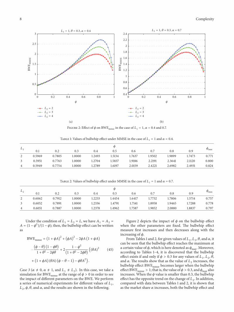
Figure 2: Effect of 𝜙 on BWEmmse in the case of 𝐿1 = 1, 𝛼 = 0.4 and 0.7.

Table 1: Values of bullwhip effect under MMSE in the case of 𝐿1 = 1 and 𝛼 = 0.4.𝐿2 𝜙 𝜙max0.1 0.2 0.3 0.4 0.5 0.6 0.7 0.8 0.92 0.5969 0.7805 1.0000 1.2493 1.5134 1.7637 1.9502 1.9899 1.7473 0.7713 0.5951 0.7763 1.0000 1.2704 1.5837 1.9186 2.2191 2.3641 2.1120 0.8004 0.5949 0.7754 1.0000 1.2789 1.6197 2.0159 2.4221 2.6982 2.4931 0.824

Table 2: Values of bullwhip effect under MMSE in the case of 𝐿1 = 1 and 𝛼 = 0.7.𝐿2 𝜙 𝜙max0.1 0.2 0.3 0.4 0.5 0.6 0.7 0.8 0.92 0.6062 0.7912 1.0000 1.2233 1.4454 1.6417 1.7732 1.7806 1.5714 0.7573 0.6052 0.7891 1.0000 1.2336 1.4791 1.7141 1.8958 1.9465 1.7288 0.7784 0.6051 0.7887 1.0000 1.2378 1.4962 1.7587 1.9852 2.0880 1.8837 0.797

Under the condition of 𝐿1 = 𝐿2 = 𝐿, we have 𝐴1 = 𝐴2 =𝐴 = (1 − 𝜙𝐿)/(1 − 𝜙); then, the bullwhip effect can be writtenas

BWEmmse = (1 + 𝜙𝐴)2 + (𝜙𝐴)2 − 2𝜙𝐴 (1 + 𝜙𝐴)⋅ (𝜙 − 𝜃) (1 − 𝜙𝜃)1 + 𝜃2 − 2𝜙𝜃 + 2 1 − 𝜙2(1 + 𝜃2 − 2𝜙𝜃) ((𝜃𝐴)2+ (1 + 𝜙𝐴) (𝜃𝐴) (𝜙 − 𝜃 − 1) − 𝜙𝜃𝐴2) .

(45)

Case 3 (𝛼 ̸= 0, 𝛼 ̸= 1, and 𝐿1 ̸= 𝐿2). In this case, we take asimulation for BWEmmse at the range of 𝜙 > 0 in order to seethe impact of different parameters on the BWE. We performa series of numerical experiments for different values of 𝐿1,𝐿2, 𝜙, 𝜃, and 𝛼, and the results are shown in the following.

Figure 2 depicts the impact of 𝜙 on the bullwhip effectwhen the other parameters are fixed. The bullwhip effectmeasure first increases and then decreases along with theincreasing of 𝜙.

From Tables 1 and 2, for given values of 𝐿1, 𝐿2, 𝜃, and 𝛼, itcan be seen that the bullwhip effect reaches the maximum ata certain value of 𝜙, which is here denoted as 𝜙max. Moreover,according to Tables 1–4, it is discovered that the bullwhipeffect exists if and only if 𝜙 > 0.3 for any values of 𝐿1, 𝐿2, 𝜃,and 𝛼. The results show that as the value of 𝐿2 increases, thebullwhip effect BWEmmse becomes larger when the bullwhipeffect BWEmmse > 1; that is, the value of𝜙 > 0.3, and𝜙max alsoincreases. When the 𝜙 value is smaller than 0.3, the bullwhipeffect has the opposite trend on the change of 𝐿2. In addition,compared with data between Tables 1 and 2, it is shown thatas the market share 𝛼 increases, both the bullwhip effect and

Complexity 9

Table 3: Values of bullwhip effect under MMSE in the case of 𝐿2 = 1 and 𝛼 = 0.4.𝐿1 𝜙 𝜙max0.1 0.2 0.3 0.4 0.5 0.6 0.7 0.8 0.92 0.6031 0.7877 1.0000 1.2319 1.4678 1.6816 1.8308 1.8483 1.6279 0.7623 0.6018 0.7848 1.0000 1.2458 1.5134 1.7804 1.9995 2.0789 1.8489 0.7874 0.6017 0.7842 1.0000 1.2514 1.5366 1.8417 2.1241 2.2789 2.0713 0.808

Table 4: Values of bullwhip effect under MMSE in the case of 𝐿2 = 1 and 𝛼 = 0.7.𝐿1 𝜙 𝜙max0.1 0.2 0.3 0.4 0.5 0.6 0.7 0.8 0.92 0.5939 0.7770 1.0000 1.2580 1.5366 1.8058 2.0120 2.0639 1.8101 0.7753 0.5917 0.7720 1.0000 1.2828 1.6197 1.9903 2.3350 2.5169 2.2550 0.8054 0.5915 0.7711 1.0000 1.2928 1.6623 2.1071 2.5812 2.9266 2.7274 0.829

𝜙max decrease, at the fixed values of𝜙, 𝐿1, and𝐿2, whichmeetsthe condition of 𝐿1 < 𝐿2.

Tables 3-4 andFigure 3 have a similar trend toTables 1 and2 and Figure 2. We set 𝐿1 > 𝐿2 in this part of simulations.Figure 3 illustrates the behavior of BWEmmse with respectto 𝜙 for fixed 𝐿1, 𝐿2, 𝜃, and 𝛼. First, it is shown that thebullwhip effect increases to amaximum and then drops as theautoregressive coefficient increases from 0 to 1. The bullwhipeffect under theMMSE forecasting method is less than 1; thatis, there is no bullwhip effect in the supply chain while 𝜙 <0.3. Second, when 𝐿1 increases and 𝐿2, 𝜃, and 𝛼 are at certainvalues, the bullwhip effect under MMSE method increases,and 𝜙max also rises for 𝜙 > 0.3. Moreover, when 𝛼 increasesfor fixed 𝐿1, 𝐿2, 𝜃, and 𝜙 under the condition of 𝐿1 >𝐿2, on the contrary, the bullwhip effect increases and 𝜙maxrises.

In a word, these results can be seen clearly from data ofTables 1–4. In conclusion, the market share of the retailerwhich has a longer lead time affects the bullwhip effect moresignificantly. From our research, we discover that the largerthe market share of the retailer with a long lead time is, thegreater the bullwhip effect is.

Next, Figure 4 shows how the market share 𝛼 affectsbullwhip effect in two cases. Further, the bullwhip effect is thelinear correlation with 𝛼. When 𝛼 goes up, the bullwhip effectdrops in Figure 4(a) for the condition of 𝐿1 < 𝐿2. However,when 𝛼 goes up, the bullwhip effect changes conversely inFigure 4(b) for the case of 𝐿1 > 𝐿2. Both figures indicate thatlarger lead time can result in a greater bullwhip effect. When𝐿1 > 𝐿2, the increasing of 𝛼means more demand needs to beforecasted in longer lead time. Thus, the lead time is criticalto the bullwhip effect.

In the simulation, the first-order moving average coeffi-cient 𝜃 affects the bullwhip effect in a way that, along with theincrease of 𝜃 from −1 to 1, the bullwhip effect first increasesslowly to themaximumwhere it corresponds to the value 𝜃maxand then decreases quickly in Figure 5. From the figure, it isobserved that when 𝜃 is almost larger than 0.6, the bullwhipeffect does not exist. Moreover, the increasing of 𝐿2 can leadto the increasing of bullwhip effect as well as 𝜃max underthe existence of the bullwhip effect. So, Figure 8 shows that

we can enlarge 𝜃 to reduce the bullwhip effect appropriatelywhen other parameters are already determined.

4.2. Behavior of the Bullwhip Effect and Parameter Analysisfor the MA. Similar to Section 4.1, there are also three casesthat we should consider. However, there is one difference ofsimulation: that we need to consider the whole range of 𝜙from −1 to 1 in this part.

Case 1 (𝛼 = 0 or 𝛼 = 1). When the market share of retailer iszero or one, it means there is only one retailer in the supplychain. We do not study this case in our paper.

Case 2 (𝐿1 = 𝐿2 = 𝐿). In the case of 𝐿1 = 𝐿2 = 𝐿, (35) can bewritten by simplification as

BWEMA = (1 + 𝐿𝑘)2 + (𝐿𝑘)

2

− 2𝐿𝑘 (1 + 𝐿𝑘) 𝜙𝑘−1 (𝜙 − 𝜃) (1 − 𝜙𝜃)1 + 𝜃2 − 2𝜙𝜃 .(46)

The bullwhip effect has no effect with the market share 𝛼from (46).

Case 3 (𝛼 ̸= 0, 𝛼 ̸= 1, and 𝐿1 ̸= 𝐿2). When we set 𝛼 ̸= 0,𝛼 ̸= 1, and 𝐿1 ̸= 𝐿2, we know the market share will affectthe bullwhip effect. Next, it is studied how the parametersinfluence the bullwhip effect under the MA forecastingtechnique by simulations on the base of the expression of (35).

As shown in Figure 6, the bullwhip effect varies differentlywith respect to the first autoregressive coefficient under thedifferent value of 𝑘. In this figure, we fix the values of 𝐿1 = 1,𝜃 = 0.3, and 𝛼 = 0.4 and run a function of 𝜙 for 𝐿2 = 2, 3,and 4, with 𝑘 = 4 and 5. The bullwhip effect first increases tothe maximum and then decreases quickly with the increasingof 𝜙 for even 𝑘. When 𝜙 = −1 or 𝜙 = 1, the values of thebullwhip effect are both one. Likewise, for odd 𝑘, the bullwhipeffect first quickly decreases to a stable value and then alsodecreases with the continuous increase of 𝜙. When 𝜙 is nearnegative one, the bullwhip effect is most pronounced.

10 Complexity

1

2

L2 = 1, = 0.3, = 0.4

L1 = 2

L1 = 3

L1 = 4

0.2 0.4 0.6 0.8 100.4

0.6

0.8

1.2

1.4

1.6

＂７

％－

－３％

1.8

2.2

2.4

(a)

L2 = 1, = 0.3, = 0.7

L1 = 2

L1 = 3

L1 = 4

0.2 0.4 0.6 0.8 100

0.5

1

1.5

＂７

％－

－３％

2

2.5

3

(b)

Figure 3: Effect of 𝜙 on BWEmmse in the case of 𝐿2 = 1, 𝛼 = 0.4 and 0.7.

L2 = 2

L2 = 3

L2 = 4

L1 = 1, = 0.6, = 0.3

1.5

1.6

1.7

1.8

1.9

2

2.1

2.2

2.3

2.4

＂７

％M

MSE

0.2 0.4 0.6 0.8 10

(a)

L1 = 2

L1 = 3

L1 = 4

0.2 0.4 0.6 0.8 10

1.5

1.6

1.7

1.8

1.9

2

2.1

2.2

2.3

2.4

＂７

％M

MSE

L2 = 1, = 0.6, = 0.3

(b)

Figure 4: The bullwhip effect corresponding to 𝛼 under the MMSE in case of 𝐿1 < 𝐿2.

Moreover, BWEMA is a function of 𝐿2 and increases as thelead time 𝐿2 increases. Equation (36) shows that the behaviorof 𝐿1 is the same as 𝐿1. So, the bullwhip effect increasesunconditionally with the increasing of the lead time.

Figure 7(a) mainly depicts the influence of market shareon the bullwhip effect. We set 𝐿1 < 𝐿2 in Figure 7(a) and𝐿1 > 𝐿2 in Figure 7(b) when other parameters are fixed.Figure 7(a) shows that the bullwhip effect decreases as themarket share 𝛼 increases. And, however, Figure 7(b) shows

that the bullwhip effect increases as the market share 𝛼increases. In a word, when the market share of the retailerwhich has a longer lead time increases, the bullwhip effectincreases too.

From the two figures, we also observe that the bullwhipeffect under the MA forecasting method is approximatelysymmetrical about 𝜙 when the span 𝑘 is even.

The first-order moving average coefficient 𝜃 has a simplerelationship with the bullwhip effect. In Figure 8, the larger

Complexity 11

0

0.5

1

1.5

2

2.5

3

＂７

％M

MSE

−0.5 0 0.5 1−1

L2 = 2

L2 = 3

L2 = 4

L1 = 1, = 0.6, = 0.4

Figure 5: Effect of 𝜃 on the bullwhip effect under theMMSEmethodfor different 𝛼.

1

1.5

2

2.5

3

3.5

4

4.5

＂７

％M

A

0.40.2 0.80.60 1−0.6−0.8 −0.4−1 −0.2

L1 = 1, = 0.3, = 0.4

L2 = 2 (k = 5)

L2 = 3 (k = 5)

L2 = 4 (k = 5)

L2 = 2 (k = 4)

L2 = 3 (k = 4)

L2 = 4 (k = 4)

Figure 6: Effect of 𝜙 on the bullwhip effect under the MA methodfor different 𝐿2 and 𝑘.

the value of 𝜃 from −1 to 1, the greater the bullwhip effect. So,in the supply chain, we can reduce 𝜃 to decrease the bullwhipeffect.The span 𝑘 is negative with the bullwhip effect, and theincreasing of 𝑘 can reduce BWEMA.

4.3. Behavior of the Bullwhip Effect and Parameter Analysis forthe ES. Based on the analytical expression of BWEES, thereare also three cases that we should consider similar to theMMSE and MAmethods.

= 0.3

= 0.5

= 0.8

−0.5 0 0.5 1−1

0.8

1

1.2

1.4

1.6

1.8

2

2.2

2.4

2.6

＂７

％M

A

L1 = 1, L2 = 2, = 0.3, k = 4

(a)

= 0.3

= 0.5

= 0.8

−0.5 0 0.5 1−1

1

1.5

2

2.5＂７

％M

AL1 = 2, L2 = 1, = 0.3, k = 4

(b)

Figure 7: Effect of 𝜙 on the bullwhip effect for different 𝛼 under𝐿1 < 𝐿2 and 𝐿1 > 𝐿2.

Case 1 (𝛼 = 0 or 𝛼 = 1). Here, the conclusion is identical tothe cases of MMSE and MAmethod.

Case 2 (𝐿1 = 𝐿2 = 𝐿, and 𝜆1 = 𝜆2 = 𝜆). We set two retailershaving the same smoothing exponent; then, when 𝐿1 = 𝐿2 =𝐿, the market share 𝛼 has no influence on the bullwhip effect.

Case 3 (𝛼 ̸= 0, 𝛼 ̸= 1, and 𝐿1 ̸= 𝐿2 or 𝜆1 ̸= 𝜆2). In order todiscuss the impact of market share 𝛼 on the bullwhip effect,we make the specific rules as 𝐿1 ̸= 𝐿2 and 𝜆1 ̸= 𝜆2. Bynumerical simulations, we will study the changes of BWEES.

12 Complexity

1.6

1.8

2

2.2

2.4

2.6

2.8

3

＂７

％M

A

−0.5 0 0.5 1−1

L1 = 1, L2 = 2, = 0.4, = 0.6

k = 3

k = 4

k = 5

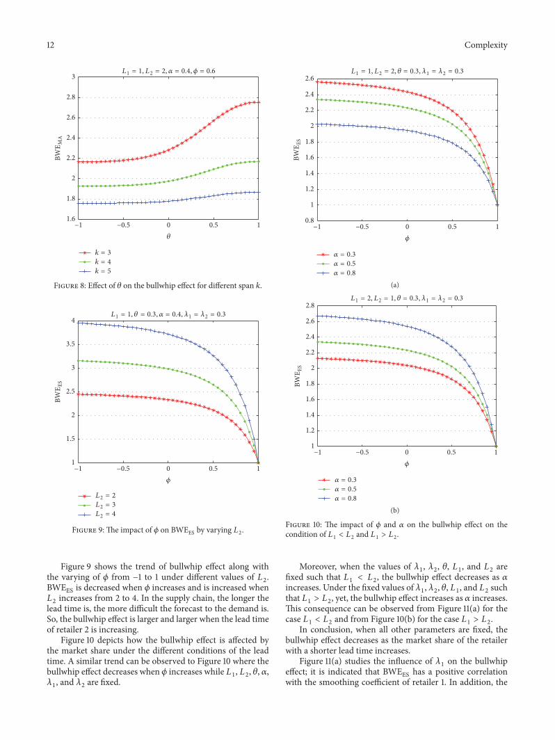
Figure 8: Effect of 𝜃 on the bullwhip effect for different span 𝑘.

−0.5 0 0.5 1−1

L2 = 2

L2 = 3

L2 = 4

1

1.5

2

2.5

3

3.5

4

＂７

％％３

L1 = 1, = 0.3, = 0.4, 1 = 2 = 0.3

Figure 9: The impact of 𝜙 on BWEES by varying 𝐿2.

Figure 9 shows the trend of bullwhip effect along withthe varying of 𝜙 from −1 to 1 under different values of 𝐿2.BWEES is decreased when 𝜙 increases and is increased when𝐿2 increases from 2 to 4. In the supply chain, the longer thelead time is, the more difficult the forecast to the demand is.So, the bullwhip effect is larger and larger when the lead timeof retailer 2 is increasing.

Figure 10 depicts how the bullwhip effect is affected bythe market share under the different conditions of the leadtime. A similar trend can be observed to Figure 10 where thebullwhip effect decreases when 𝜙 increases while 𝐿1, 𝐿2, 𝜃, 𝛼,𝜆1, and 𝜆2 are fixed.

0.8

1

1.2

1.4

1.6

1.8

2

2.2

2.4

2.6

＂７

％％３

= 0.3

= 0.5

= 0.8

L1 = 1, L2 = 2, = 0.3, 1 = 2 = 0.3

−0.5 0 0.5 1−1

(a)

= 0.3

= 0.5

= 0.8

L1 = 2, L2 = 1, = 0.3, 1 = 2 = 0.3

1

1.2

1.4

1.6

1.8

2

2.2

2.4

2.6

2.8＂７

％％３

−0.5 0 0.5 1−1

(b)

Figure 10: The impact of 𝜙 and 𝛼 on the bullwhip effect on thecondition of 𝐿1 < 𝐿2 and 𝐿1 > 𝐿2.

Moreover, when the values of 𝜆1, 𝜆2, 𝜃, 𝐿1, and 𝐿2 arefixed such that 𝐿1 < 𝐿2, the bullwhip effect decreases as 𝛼increases. Under the fixed values of 𝜆1, 𝜆2, 𝜃, 𝐿1, and 𝐿2 suchthat 𝐿1 > 𝐿2, yet, the bullwhip effect increases as 𝛼 increases.This consequence can be observed from Figure 11(a) for thecase 𝐿1 < 𝐿2 and from Figure 10(b) for the case 𝐿1 > 𝐿2.

In conclusion, when all other parameters are fixed, thebullwhip effect decreases as the market share of the retailerwith a shorter lead time increases.

Figure 11(a) studies the influence of 𝜆1 on the bullwhipeffect; it is indicated that BWEES has a positive correlationwith the smoothing coefficient of retailer 1. In addition, the

Complexity 13

L2 = 1

L2 = 2

L2 = 3

1

1.5

2

2.5

3

3.5

4

4.5

5＂７

％％３

L1 = 2, = 0.3, = 0.6, = 0.4, 2 = 0.3

10 0.6 0.80.2 0.41

(a)

L1 = 2, = 0.6, = 0.4, 1 = 2 = 0.3

1.6

1.8

2

2.2

2.4

2.6

2.8

3

3.2

3.4

3.6

＂７

％％３

0 1−1 0.5−0.5

L2 = 1

L2 = 2

L2 = 3

(b)

Figure 11: The impact of the smoothing coefficient 𝜆1 and 𝜃 on BWEES for different 𝐿2.

trend of BWEES is roughly the same for different 𝐿2. That is,the influence of the smoothing coefficient 𝜆1 on the bullwhipeffect is determinate regardless of the measurement of 𝐿1 and𝐿2.

Figure 11(b) indicates the behavior of the bullwhip effectwith regard to 𝜃 for fixed values of other parameters.The bull-whip effect is increased slowly along with the increasing of 𝜃from −1 to 0; however, it increases quickly when 𝜃 increasesfrom 0 to 1. Some other information can be discovered fromFigure 11(b). The larger the value of 𝐿2 is, the faster thebullwhip effect increases as 𝜃 increases.4.4. Comparison of the Bullwhip Effect by Three ForecastingMethods. We study the bullwhip effect using three forecast-ing methods in Sections of 4.1–4.3. Next, we will compare thedifferent influences of MMSE, MA, and ES on the bullwhipeffect. For the comparability of the MA and ES methods, weset a constraint on the span 𝑘 of MA and the smoothingfactors 𝜆1 and 𝜆2. According to Zhang [8], we obtain that thesmoothing exponents are fixed as 𝜆1 = 𝜆2 = 2/(𝑘 + 1). Thismeans the average data ages are the same for the MA and ESforecasting method. Further, we know 𝜙 + 𝜆2 − 1 ̸= 0 fromthe expression of the bullwhip effect (see (46)) under the ESforecasting method.

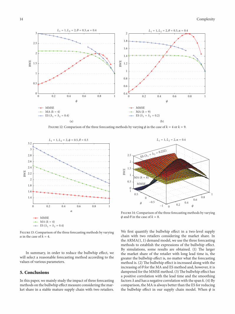
Figure 12 depicts the difference of the three forecastingmethods on measuring the bullwhip effect by varying 𝜙 fordifferent 𝑘 and 𝜆.We observe that the bullwhip effectmeasureof MA is always smaller than that of ES nomatter what 𝜙 is aslong as 𝜆1 = 𝜆2 = 2/(𝑘 + 1). It can be seen that the bullwhipeffect under the MMSE forecasting method does not existwhen 𝜙 ≤ 0.3 from the two figures.The bullwhip effect for thethree forecasting methods converges to one as 𝜙 approachesone.

Moreover, for fixed values of 𝛼, 𝜃, 𝐿1, and 𝐿2, BWEMMSEis the least when 𝜙 is smaller than a certain value, called 𝜙1.After 𝜙 becomes larger than 𝜙1 and smaller than anothercertain value, called𝜙2, BWEMA is the smallest andBWEMMSEis lower than BWEES. When 𝜙 is larger than 𝜙2, BWEMMSE isthe largest compared to the other two methods. In general,while 𝜙 is lower than 𝜙1, the MMSE method is the best forreducing the bullwhip effect, and while 𝜙 is higher than 𝜙1,the MA method is the best.

However, comparing the two figures, we find that as thespan 𝑘 increases, the bullwhip effects for the three forecastingmethods overall decrease, and the values of 𝜙1 and 𝜙2 arelessened. This phenomenon reveals that when we choose alarger span 𝑘, the extent of 𝜙 is larger for the MAwhich is thebest method to predict the bullwhip effect.

In Figure 13, we set 𝜙 = 0.5, 𝜃 = 0.3, 𝐿1 = 1, 𝐿2 = 2, 𝜆1 =𝜆2 = 0.4, and 𝑘 = 4 and then study the bullwhip effect forthe three forecasting methods under the condition of variousmarket shares 𝛼. We observe that the bullwhip effect is thesmallest by theMMSE forecastingmethodwhatever𝛼 is. Andthe bullwhip effect under the ESmethod is theworst whatever𝛼 is.This conclusion is related to the value of 𝜙whenwe selecta certain 𝑘.

Figure 14 shows the curved surface of the bullwhip effectby varying 𝜙 and 𝜃 for the three forecasting methods. It isobserved that BWEES is always larger than BWEMA whatever𝜃 is as long as 𝜆1 = 𝜆2 = 2/(𝑘 + 1) for the fixed value of𝜙. When 𝜃 increases from −1 to 1, BWEMA is the smallestwhile 𝜃 is less than a certain value, and BWEMMSE is thebest while 𝜃 is more than that certain value. In addition,there is also a phenomenon where BWEMMSE is all alongthe largest for any value of 𝜙 when 𝜃 approaches negativeone.

14 Complexity

MMSEMA (k = 4)ES (1 = 2 = 0.4)

0

0.5

1

1.5

2

2.5

3BW

EL1 = 1, L2 = 2, = 0.3, = 0.4

0.2 0.4 0.6 0.8 10

(a)

0.4

0.6

0.8

1

1.2

1.4

1.6

1.8

2

BWE

MMSEMA (k = 9)ES (1 = 2 = 0.2)

L1 = 1, L2 = 2, = 0.3, = 0.4

0.2 0.4 0.6 0.8 10

(b)

Figure 12: Comparison of the three forecasting methods by varying 𝜙 in the case of 𝑘 = 4 or 𝑘 = 9.

MMSE

1.4

1.6

1.8

2

2.2

2.4

2.6

2.8

3

3.2

BWE

10 0.6 0.80.2 0.4

MA (k = 4)ES (1 = 2 = 0.4)

L1 = 1, L2 = 2, = 0.5, = 0.3

Figure 13: Comparison of the three forecasting methods by varying𝛼 in the case of 𝑘 = 4.

In summary, in order to reduce the bullwhip effect, wewill select a reasonable forecasting method according to thevalues of various parameters.

5. Conclusions

In this paper, we mainly study the impact of three forecastingmethods on the bullwhip effectmeasure considering themar-ket share in a stable mature supply chain with two retailers.

0

1

−1

0

1

MMSE

MA (k = 8)

L1 = 1, L2 = 2, = 0.4

ES (1= 2

= 0.222)

−0.5

0.5

0.2

0.80.6

0.4

0

0.5

1

1.5

2

2.5

BWE

Figure 14: Comparison of the three forecasting methods by varying𝜙 and 𝜃 in the case of 𝑘 = 8.

We first quantify the bullwhip effect in a two-level supplychain with two retailers considering the market share. Inthe ARMA(1, 1) demand model, we use the three forecastingmethods to establish the expressions of the bullwhip effect.By simulations, some results are obtained. (1) The largerthe market share of the retailer with long lead time is, thegreater the bullwhip effect is, no matter what the forecastingmethod is. (2)The bullwhip effect is increased along with theincreasing of 𝜃 for the MA and ES method and, however, it isdampened for theMMSEmethod. (3)The bullwhip effect hasa positive correlation with the lead time and the smoothingfactors 𝜆 and has a negative correlationwith the span 𝑘. (4) Bycomparison, theMA is always better than the ES for reducingthe bullwhip effect in our supply chain model. When 𝜙 is

Complexity 15

lower than a certain value, the MMSE method is the best forreducing the bullwhip effect; otherwise, the MA method isthe best.

Our findings give some useful insights for supply chainmanagers in the consumer electronics industry. Firstly, theretailers shouldmake it clearwhat kind of pattern the demandprocess follows and choose a suitable forecasting methodto dampen the bullwhip effect. Secondly, the manufacturershould paymore attention to the retailer who occupies a largemarket share on purpose and reduce its lead time to dampenthe bullwhip effect.

From the view of entropy, we see that the autocorrelationcoefficient can impact the uncertainty of the order. Theminimum of the entropy is around 𝜙 = 0.672, and themaximum of the entropy is around 𝜙 = 1.

The research presented in this paper proposes severalfuture directions for improvement of our understanding ofmarket share. First, we can further study the effect of unfixedmarket share on the bullwhip effect in an unstable supplychain. Second, we only consider the order-up-to inventorypolicy and three traditional demand forecasting methods.Therefore, other new forecast methods and complex inven-tory policies can be studied in future research. Furthermore,price is the key factor on the bullwhip effect. So, introducingthe retailer’s price into the demand model to analyze thecomplexity and stability of the supply chain system is anotherfuture direction.

Appendix

A. A Proof of Proposition 1

Var (𝜀𝑡−1) = Var (𝜀𝑡−2) = Var (𝜀𝑡)= 1 − 𝜙21 + 𝜃2 − 2𝜙𝜃 Var (𝑑𝑡) . (A.1)

According to Feng and Ma [17], there is

Cov (𝑑𝑡−1, 𝑑𝑡−𝑘−1) = 𝜙𝑘−1 (𝜙 − 𝜃) (1 − 𝜙𝜃)1 + 𝜃2 − 2𝜙𝜃 Var (𝑑𝑡) . (A.2)

According to Duc et al. [16], we have

Cov (𝑑𝑡−1, 𝜀𝑡−1) = Var (𝜀𝑡−1) ,Cov (𝑑𝑡−1, 𝜀𝑡−2) = (𝜙 − 𝜃)Var (𝜀𝑡−1) . (A.3)

Take the variance of (27); we get

Var (𝑞𝑡) = Var ((1 + 𝛼𝜙𝐴1 + (1 − 𝛼) 𝜙𝐴2) 𝑑𝑡−1− (𝛼𝜙𝐴1 + (1 − 𝛼) 𝜙𝐴2) 𝑑𝑡−2− (𝛼𝜃𝐴1 + (1 − 𝛼) 𝜃𝐴2) 𝜀𝑡−1+ (𝛼𝜃𝐴1 + (1 − 𝛼) 𝜃𝐴2) 𝜀𝑡−2)= Var ((1 + 𝛼𝜙𝐴1 + (1 − 𝛼) 𝜙𝐴2) 𝑑𝑡−1)

+ Var ((1 − 𝛼) (𝜙𝐴2 + 1) 𝑑𝑡−2)+ Var ((𝛼𝜃𝐴1 + (1 − 𝛼) 𝜃𝐴2) 𝜀𝑡−1)+ Var ((𝛼𝜃𝐴1 + (1 − 𝛼) 𝜃𝐴2) 𝜀𝑡−2) − 2 (1 + 𝛼𝜙𝐴1+ (1 − 𝛼) 𝜙𝐴2) (𝛼𝜙𝐴1 + (1 − 𝛼) 𝜙𝐴2)⋅ Cov (𝑑𝑡−1, 𝑑𝑡−2) − 2 (1 + 𝛼𝜙𝐴1 + (1 − 𝛼) 𝜙𝐴2)⋅ (𝛼𝜃𝐴1 + (1 − 𝛼) 𝜃𝐴2)Cov (𝑑𝑡−1, 𝜀𝑡−1) + 2 (1+ 𝛼𝜙𝐴1 + (1 − 𝛼) 𝜙𝐴2) (𝛼𝜃𝐴1 + (1 − 𝛼) 𝜃𝐴2)⋅ Cov (𝑑𝑡−1, 𝜀𝑡−2) + 2 (𝛼𝜙𝐴1 + (1 − 𝛼) 𝜙𝐴2)⋅ (𝛼𝜃𝐴1 + (1 − 𝛼) 𝜃𝐴2)Cov (𝑑𝑡−2, 𝜀𝑡−1)− 2 (𝛼𝜙𝐴1 + (1 − 𝛼) 𝜙𝐴2) (𝛼𝜃𝐴1 + (1 − 𝛼) 𝜃𝐴2)⋅ Cov (𝑑𝑡−2, 𝜀𝑡−2) − 2 (𝛼𝜃𝐴1 + (1 − 𝛼) 𝜃𝐴2)2⋅ Cov (𝜀𝑡−1, 𝜀𝑡−2) .

(A.4)

Bring (A.1)–(A.3) into (A.4) and simplify the originalequation; we can get the variance of the order quantity underthe MMSE forecasting method as follows:

Var (𝑞𝑡) = ((1 + 𝛼𝜙𝐴1 + (1 − 𝛼) 𝜙𝐴2)2 + (𝛼𝜙𝐴1+ (1 − 𝛼) 𝜙𝐴2)2)Var (𝑑𝑡) + 2 (𝛼𝜃𝐴1 + (1 − 𝛼)⋅ 𝜃𝐴2)2 Var (𝜀𝑡) − 2 (1 + 𝛼𝜙𝐴1 + (1 − 𝛼) 𝜙𝐴2)⋅ (𝛼𝜙𝐴1 + (1 − 𝛼) 𝜙𝐴2) (𝜙 − 𝜃) (1 − 𝜙𝜃)1 + 𝜃2 − 2𝜙𝜃 Var (𝑑𝑡)− 2 (1 + 𝛼𝜙𝐴1 + (1 − 𝛼) 𝜙𝐴2) (𝛼𝜃𝐴1 + (1 − 𝛼)⋅ 𝜃𝐴2)Var (𝜀𝑡−1) + 2 (1 + 𝛼𝜙𝐴1 + (1 − 𝛼) 𝜙𝐴2)⋅ (𝛼𝜃𝐴1 + (1 − 𝛼) 𝜃𝐴2) (𝜙 − 𝜃)Var (𝜀𝑡−1)− 2 (𝛼𝜙𝐴1 + (1 − 𝛼) 𝜙𝐴2) (𝛼𝜃𝐴1 + (1 − 𝛼) 𝜃𝐴2)⋅ Var (𝜀𝑡−2) = [(1 + 𝛼𝜙𝐴1 + (1 − 𝛼) 𝜙𝐴2)2+ (𝛼𝜙𝐴1 + (1 − 𝛼) 𝜙𝐴2)2 − 2 (1 + 𝛼𝜙𝐴1+ (1 − 𝛼) 𝜙𝐴2) (𝛼𝜙𝐴1 + (1 − 𝛼) 𝜙𝐴2)⋅ (𝜙 − 𝜃) (1 − 𝜙𝜃)1 + 𝜃2 − 2𝜙𝜃 + 2⋅ 1 − 𝜙21 + 𝜃2 − 2𝜙𝜃 ((𝛼𝜃𝐴1 + (1 − 𝛼) 𝜃𝐴2)2− (1 + 𝛼𝜙𝐴1 + (1 − 𝛼) 𝜙𝐴2)⋅ (𝛼𝜃𝐴1 + (1 − 𝛼) 𝜃𝐴2)

16 Complexity

+ (1 + 𝛼𝜙𝐴1 + (1 − 𝛼) 𝜙𝐴2)⋅ (𝛼𝜃𝐴1 + (1 − 𝛼) 𝜃𝐴2) (𝜙 − 𝜃)− (𝛼𝜙𝐴1 + (1 − 𝛼) 𝜙𝐴2) (𝛼𝜃𝐴1 + (1 − 𝛼) 𝜃𝐴2))]⋅ Var (𝑑𝑡) .

(A.5)

This completes the proof of Proposition 1.

B. A Proof of Proposition 2

The variance of the total order quantity under the MAforecasting method can be derived from (33) as follows:

Var (𝑞𝑡) = Var ((1 + 𝛼𝐿1𝑘 + (1 − 𝛼) 𝐿2𝑘 ) 𝑑𝑡−1− (𝛼𝐿1𝑘 + (1 − 𝛼) 𝐿2𝑘 ) 𝑑𝑡−𝑘−1) = (1 + 𝛼𝐿1𝑘+ (1 − 𝛼) 𝐿2𝑘 )2 Var (𝑑𝑡−1) + (𝛼𝐿1𝑘 + (1 − 𝛼) 𝐿2𝑘 )2

⋅ Var (𝑑𝑡−𝑘−1) − 2 (1 + 𝛼𝐿1𝑘 + (1 − 𝛼) 𝐿2𝑘 ) (𝛼𝐿1𝑘+ (1 − 𝛼) 𝐿2𝑘 )Cov (𝑑𝑡−1, 𝑑𝑡−𝑘−1) .

(B.1)

According to (A.2), the variance can be simplified as

Var (𝑞𝑡) = [(1 + 𝛼𝐿1𝑘 + (1 − 𝛼) 𝐿2𝑘 )2

+ (𝛼𝐿1𝑘 + (1 − 𝛼) 𝐿2𝑘 )2

− 2 (1 + 𝛼𝐿1𝑘 + (1 − 𝛼) 𝐿2𝑘 ) (𝛼𝐿1𝑘 + (1 − 𝛼) 𝐿2𝑘 )⋅ 𝜙𝑘−1 (𝜙 − 𝜃) (1 − 𝜙𝜃)1 + 𝜃2 − 2𝜙𝜃 ]Var (𝑑𝑡) .

(B.2)

This completes the proof of Proposition 2.

C. A Proof of Proposition 3

The variance of the total order quantity under the ESforecasting method can be derived from (42) as follows:

Var (𝑞𝑡) = Var ((1 + 𝛼𝜆1𝐿1 + (1 − 𝛼) 𝜆2𝐿2) 𝑑𝑡−1− 𝜆1𝐿1𝑑1,𝑡−1 − 𝜆2𝐿2𝑑2,𝑡−1) = (1 + 𝛼𝜆1𝐿1+ (1 − 𝛼) 𝜆2𝐿2)2 Var (𝑑𝑡−1) + (𝜆1𝐿1)2 Var (𝑑1,𝑡−1)

+ (𝜆2𝐿2)2 Var (𝑑2,𝑡−1) − 2 (1 + 𝛼𝜆1𝐿1+ (1 − 𝛼) 𝜆2𝐿2) 𝜆1𝐿1Cov (𝑑𝑡−1, 𝑑1,𝑡−1) − 2 (1+ 𝛼𝜆1𝐿1 + (1 − 𝛼) 𝜆2𝐿2) 𝜆2𝐿2Cov (𝑑𝑡−1, 𝑑2,𝑡−1)+ 2𝜆1𝐿1𝜆2𝐿2Cov (𝑑1,𝑡−1, 𝑑2,𝑡−1) ,

(C.1)

where

Var (𝑑1,𝑡−1) = Var(∞∑𝑖=0

𝜆1 (1 − 𝜆1)𝑖 𝑑1,𝑡−𝑖−2)= 𝜆21 ∞∑𝑖=0

(1 − 𝜆1)2𝑖 Var (𝑑1,𝑡−𝑖−2)+ 2𝜆21 ∞∑

𝑖=0

∞∑𝑗>𝑖

(1 − 𝜆1)𝑖 (1 − 𝜆1)𝑗

⋅ Cov (𝑑1,𝑡−𝑖−2, 𝑑1,𝑡−𝑗−2) = 𝜆21 ∞∑𝑖=0

(1 − 𝜆1)2𝑖

⋅ 𝛼2Var (𝑑𝑡−𝑖−2) + 2𝜆21𝛼2 ∞∑𝑖=0

∞∑𝑗>𝑖

(1 − 𝜆1)𝑖+𝑗

⋅ Cov (𝑑𝑡−𝑖−2, 𝑑𝑡−𝑗−2) = 𝛼2𝜆21 1𝜆1 (2 − 𝜆1)Var (𝑑𝑡)+ 2𝜆21𝛼2 ∞∑

𝑖=0

∞∑𝑗>𝑖

(1 − 𝜆1)𝑖+𝑗 𝜙𝑗−𝑖−1

⋅ (𝜙 − 𝜃) (1 − 𝜙𝜃)1 + 𝜃2 − 2𝜙𝜃 Var (𝑑𝑡) = 𝛼2𝜆21Var (𝑑𝑡)⋅ [ 1𝜆1 (2 − 𝜆1) + 2(𝜙 − 𝜃) (1 − 𝜙𝜃)(1 + 𝜃2 − 2𝜙𝜃)⋅ (1 − 𝜆1)𝜆1 (2 − 𝜆1) (1 − (1 − 𝜆1) 𝜙)] = 𝜆1𝛼22 − 𝜆1 [1+ 2 (1 − 𝜆1)1 − (1 − 𝜆1) 𝜙

(𝜙 − 𝜃) (1 − 𝜙𝜃)(1 + 𝜃2 − 2𝜙𝜃) ]Var (𝑑𝑡) ,

(C.2)

and, similarly, we have

Var (𝑑2,𝑡−1) = Var(∞∑𝑖=0

𝜆2 (1 − 𝜆2)𝑖 𝑑2,𝑡−𝑖−2)= 𝜆22 ∞∑𝑖=0

(1 − 𝜆2)2𝑖 (1 − 𝛼)2 Var (𝑑𝑡−𝑖−2) + 2𝜆22 (1− 𝛼)2 ∞∑

𝑖=0

∞∑𝑗>𝑖

(1 − 𝜆2)𝑖+𝑗 Cov (𝑑𝑡−𝑖−2, 𝑑𝑡−𝑗−2) = (1− 𝛼)2 𝜆22Var (𝑑𝑡) [ 1𝜆2 (2 − 𝜆2) + 2

Complexity 17

⋅ (𝜙 − 𝜃) (1 − 𝜙𝜃)(1 + 𝜃2 − 2𝜙𝜃) (1 − 𝜆2)𝜆2 (2 − 𝜆2) (1 − (1 − 𝜆2) 𝜙)]= 𝜆2 (1 − 𝛼)22 − 𝜆2 [1 + 2 (1 − 𝜆2)1 − (1 − 𝜆2) 𝜙⋅ (𝜙 − 𝜃) (1 − 𝜙𝜃)(1 + 𝜃2 − 2𝜙𝜃) ]Var (𝑑𝑡) ,

Cov (𝑑𝑡−1, 𝑑1,𝑡−1) = Cov(𝑑𝑡−1,∞∑𝑖=0

𝜆1 (1 − 𝜆1)𝑖 𝑑1,𝑡−𝑖−2) = 𝛼𝜆1 ∞∑𝑖=0

(1 − 𝜆1)𝑖

⋅ Cov (𝑑𝑡−1, 𝑑𝑡−𝑖−2) = 𝛼𝜆1 ∞∑𝑖=0

(1 − 𝜆1)𝑖 𝜙𝑖

⋅ (𝜙 − 𝜃) (1 − 𝜙𝜃)1 + 𝜃2 − 2𝜙𝜃 Var (𝑑𝑡) = 𝛼𝜆11 − (1 − 𝜆1) 𝜙⋅ (𝜙 − 𝜃) (1 − 𝜙𝜃)1 + 𝜃2 − 2𝜙𝜃 Var (𝑑𝑡) ,

Cov (𝑑𝑡−1, 𝑑2,𝑡−1) = Cov(𝑑𝑡−1,∞∑𝑖=0

𝜆2 (1 − 𝜆2)𝑖 𝑑2,𝑡−𝑖−2) = (1 − 𝛼) 𝜆2 ∞∑𝑖=0

(1− 𝜆2)𝑖 Cov (𝑑𝑡−1, 𝑑𝑡−𝑖−2) = (1 − 𝛼) 𝜆21 − (1 − 𝜆2) 𝜙⋅ (𝜙 − 𝜃) (1 − 𝜙𝜃)1 + 𝜃2 − 2𝜙𝜃 Var (𝑑𝑡) ,

Cov (𝑑1,𝑡−1, 𝑑2,𝑡−1) = Cov(∞∑𝑖=0

𝜆1 (1 − 𝜆1)𝑖 𝑑1,𝑡−𝑖−2,∞∑𝑗=0

𝜆2 (1 − 𝜆2)𝑗 𝑑2,𝑡−𝑗−2) = 𝜆1𝜆2𝛼 (1 − 𝛼)

⋅ ∞∑𝑖=0

(1 − 𝜆1)𝑖 Cov(𝑑𝑡−𝑖−2, ∞∑𝑗=0

(1 − 𝜆2)𝑗 𝑑2,𝑡−𝑗−2)= 𝜆1𝜆2𝛼 (1 − 𝛼) ∞∑

𝑖=0

(1 − 𝜆1)𝑖

⋅ ∞∑𝑗=0

(1 − 𝜆2)𝑗 Cov (𝑑𝑡−𝑖−2, 𝑑𝑡−𝑗−2) = 𝜆1𝜆2𝛼 (1− 𝛼)Var (𝑑𝑡) ∞∑

𝑖=0

(1 − 𝜆1)𝑖

⋅ (𝑖−1∑𝑗=0

(1 − 𝜆2)𝑗 𝜙𝑖−𝑗−1 (𝜙 − 𝜃) (1 − 𝜙𝜃)1 + 𝜃2 − 2𝜙𝜃+ ∞∑𝑗>𝑖

(1 − 𝜆2)𝑗 𝜙𝑗−𝑖−1 (𝜙 − 𝜃) (1 − 𝜙𝜃)1 + 𝜃2 − 2𝜙𝜃+ (1 − 𝜆2)𝑖) .

(C.3)

Substituting (C.2)-(C.3) into (C.1) and simplifying theequation, we can derive the expression of the variance ofthe order quantity of two retailers under the ES forecastingmethod as follows:

Var (𝑞𝑡) = (1 + 𝛼𝜆1𝐿1 + (1 − 𝛼) 𝜆2𝐿2)2 Var (𝑑𝑡) + 𝐿21𝜆31𝛼22 − 𝜆1 [1 + 2 (1 − 𝜆1)1 − (1 − 𝜆1) 𝜙(𝜙 − 𝜃) (1 − 𝜙𝜃)(1 + 𝜃2 − 2𝜙𝜃) ]Var (𝑑𝑡)

+ 𝐿22𝜆32 (1 − 𝛼)22 − 𝜆2 [1 + 2 (1 − 𝜆2)1 − (1 − 𝜆2) 𝜙(𝜙 − 𝜃) (1 − 𝜙𝜃)(1 + 𝜃2 − 2𝜙𝜃) ]Var (𝑑𝑡) − 2 (1 + 𝛼𝜆1𝐿1 + (1 − 𝛼) 𝜆2𝐿2) 𝛼𝐿1𝜆211 − (1 − 𝜆1) 𝜙

⋅ (𝜙 − 𝜃) (1 − 𝜙𝜃)1 + 𝜃2 − 2𝜙𝜃 Var (𝑑𝑡) − 2 (1 + 𝛼𝜆1𝐿1 + (1 − 𝛼) 𝜆2𝐿2) (1 − 𝛼) 𝐿2𝜆221 − (1 − 𝜆2) 𝜙(𝜙 − 𝜃) (1 − 𝜙𝜃)1 + 𝜃2 − 2𝜙𝜃 Var (𝑑𝑡)

+ 2𝜆21𝜆22𝐿1𝐿2𝛼 (1 − 𝛼)Var (𝑑𝑡) ∞∑𝑖=0

(1 − 𝜆1)𝑖

⋅ (𝑖−1∑𝑗=0

(1 − 𝜆2)𝑗 𝜙𝑖−𝑗−1 (𝜙 − 𝜃) (1 − 𝜙𝜃)1 + 𝜃2 − 2𝜙𝜃 + ∞∑𝑗>𝑖

(1 − 𝜆2)𝑗 𝜙𝑗−𝑖−1 (𝜙 − 𝜃) (1 − 𝜙𝜃)1 + 𝜃2 − 2𝜙𝜃 + (1 − 𝜆2)𝑖) = Var (𝑑𝑡) [[(1 + 𝛼𝜆1𝐿1

+ (1 − 𝛼) 𝜆2𝐿2)2 + 𝐿21𝜆31𝛼22 − 𝜆1 (1 + 2 (1 − 𝜆1)1 − (1 − 𝜆1) 𝜙(𝜙 − 𝜃) (1 − 𝜙𝜃)(1 + 𝜃2 − 2𝜙𝜃) ) + 𝐿22𝜆32 (1 − 𝛼)22 − 𝜆2 (1

18 Complexity

+ 2 (1 − 𝜆2)1 − (1 − 𝜆2) 𝜙(𝜙 − 𝜃) (1 − 𝜙𝜃)(1 + 𝜃2 − 2𝜙𝜃) ) − 2 (1 + 𝛼𝜆1𝐿1 + (1 − 𝛼) 𝜆2𝐿2) (𝜙 − 𝜃) (1 − 𝜙𝜃)1 + 𝜃2 − 2𝜙𝜃 ( 𝛼𝐿1𝜆211 − (1 − 𝜆1) 𝜙

+ (1 − 𝛼) 𝐿2𝜆221 − (1 − 𝜆2) 𝜙) + 2𝜆21𝜆22𝐿1𝐿2𝛼 (1 − 𝛼)⋅ ∞∑𝑖=0

(1 − 𝜆1)𝑖(𝑖−1∑𝑗=0

(1 − 𝜆2)𝑗 𝜙𝑖−𝑗−1 (𝜙 − 𝜃) (1 − 𝜙𝜃)1 + 𝜃2 − 2𝜙𝜃 + ∞∑𝑗>𝑖

(1 − 𝜆2)𝑗 𝜙𝑗−𝑖−1 (𝜙 − 𝜃) (1 − 𝜙𝜃)1 + 𝜃2 − 2𝜙𝜃 + (1 − 𝜆2)𝑖)]]

= Var (𝑑𝑡) [(1 + 𝛼𝜆1𝐿1 + (1 − 𝛼) 𝜆2𝐿2)2 + 𝐿21𝜆31𝛼22 − 𝜆1 (1 + 2 (1 − 𝜆1)1 − (1 − 𝜆1) 𝜙(𝜙 − 𝜃) (1 − 𝜙𝜃)(1 + 𝜃2 − 2𝜙𝜃) ) + 𝐿22𝜆32 (1 − 𝛼)22 − 𝜆2 (1

+ 2 (1 − 𝜆2)1 − (1 − 𝜆2) 𝜙(𝜙 − 𝜃) (1 − 𝜙𝜃)(1 + 𝜃2 − 2𝜙𝜃) ) − 2 (1 + 𝛼𝜆1𝐿1 + (1 − 𝛼) 𝜆2𝐿2) (𝜙 − 𝜃) (1 − 𝜙𝜃)1 + 𝜃2 − 2𝜙𝜃 ( 𝛼𝐿1𝜆211 − (1 − 𝜆1) 𝜙

+ (1 − 𝛼) 𝐿2𝜆221 − (1 − 𝜆2) 𝜙) + 2𝜆21𝜆22𝐿1𝐿2𝛼 (1 − 𝛼)((𝜙 − 𝜃) (1 − 𝜙𝜃)1 + 𝜃2 − 2𝜙𝜃 1(𝜙 + 𝜆2 − 1) (1 − (1 − 𝜆1) 𝜙)+ 11 − (1 − 𝜆1) (1 − 𝜆2) (1 +

(𝜙 − 𝜃) (1 − 𝜙𝜃)1 + 𝜃2 − 2𝜙𝜃 ( 1 − 𝜆21 − (1 − 𝜆2) 𝜙 − 1𝜙 + 𝜆2 − 1)))] .(C.4)

This completes the proof of Proposition 3.

Conflicts of Interest

The authors declare no conflicts of interest.

Acknowledgments

This research was supported by the National Natural ScienceFoundation of China (71571131). The authors would like toappreciate Dr. Weiya Di and Dr. Xiaogang Ma’s valuableadvice and help. All authors have read and approved the finalmanuscript.

References

[1] H. L. Lee, P. Padmanabhan, and S.Whang, “Information distor-tion in a supply chain: the bullwhip effect,”Management Science,vol. 43, no. 4, pp. 546–558, 1997.

[2] H. L. Lee, P. Padmanabhan, and S. Whang, “Bullwhip Effect ina Supply Chain,” Sloan Management Review, vol. 38, no. 2, pp.93–102, 1997.

[3] J.W. Forrester, “Industrial Dynamics-AMajor Breakthrough forDecision Making,” Harvard Business Review, vol. 36, no. 4, pp.37–66, 1958.

[4] J. W. Forrester, Industrial Dynamics, MIT Press, Cambridge,Mass, USA, 1961.

[5] J. Sterman, “Optimal Policy for A Multi-product, Dynamic,Nonstationary Inventory Problem,” Management Science, vol.18, no. 12, pp. 206–222, 1989.

[6] F. Chen, Z. Drezner, J. K. Ryan, and D. Simchi-Levi, “Quantify-ing the bullwhip effect in a simple supply chain: the impact of

forecasting, lead times, and information,”Management Science,vol. 46, no. 3, pp. 436–443, 2000.

[7] F. Chen, J. K. Ryan, and D. Simchi-Levi, “The impact of expo-nential smoothing forecasts on the bullwhip effect,” NavalResearch Logistics, vol. 47, no. 4, pp. 269–286, 2000.

[8] X. Zhang, “The impact of forecasting methods on the bullwhipeffect,” International Journal of Production Economics, vol. 88,no. 1, pp. 15–27, 2004.

[9] H. L. Lee, K. C. So, andC. S. Tang, “Value of information sharingin a two-level supply chain,”Management Science, vol. 46, no. 5,pp. 626–643, 2000.

[10] H. T. Luong, “Measure of bullwhip effect in supply chains withautoregressive demand process,” European Journal of Opera-tional Research, vol. 180, no. 3, pp. 1086–1097, 2007.

[11] H. T. Luong and N. H. Phien, “Measure of bullwhip effect insupply chains: The case of high order autoregressive demandprocess,” European Journal of Operational Research, vol. 183, no.1, pp. 197–209, 2007.

[12] T. T. H. Duc, H. T. Luong, and Y. D. Kim, “Effect of the third-party warehouse on bullwhip effect and inventory cost in supplychains,” International Journal of Production Economics, vol. 124,no. 2, pp. 395–407, 2010.

[13] S. C.Graves, “A single-item inventorymodel for a nonstationarydemand process,”Manufacturing & Service OperationsManage-ment, vol. 1, no. 1, pp. 50–61, 1999.

[14] R. S. Pindyck and D. L. Rubinfeld, Econometric Models andEconomic Forecasts, IrwinMcGraw-Hill, Boston,MA, USA, 4thedition, 1998.

[15] S. M. Disney, I. Farasyn, M. Lambrecht, D. Towill, and W. VandeVelde, “Taming the bullwhip effect whilst watching customerservice in a single supply chain echelon,” European Journal ofOperational Research, vol. 173, no. 1, pp. 151–172, 2006.

[16] T. T. Duc, H. T. Luong, and Y.-D. Kim, “A measure of bullwhipeffect in supply chains with a mixed autoregressive-moving

Complexity 19

average demand process,” European Journal of OperationalResearch, vol. 187, no. 1, pp. 243–256, 2008.

[17] Y. Feng and J. H. Ma, “Demand and Forecasting in SupplyChains Based on ARMA(1, 1) Demand process,” IndustrialEngineering Journal, vol. 11, no. 5, pp. 50–55, 2008.

[18] J. H. Ma and X. G. Ma, “A comparison of bullwhip effect undervarious forecasting techniques in supply chains with two retail-ers,”Abstract and Applied Analysis, vol. 2013, Article ID 796384,14 pages, 2013.

[19] J. H. Ma and J. Zhang, “Measure of bullwhip effect consideringstochastic disturbance based on price fluctuations in a supplychain with two retailers,” Wseas Transactions on Mathematics,vol. 14, pp. 127–149, 2015.

[20] S. Bandyopadhyay and R. Bhattacharya, “A generalizedmeasureof bullwhip effect in supply chain with ARMA demand processunder various replenishment policies,” International Journal ofAdvanced Manufacturing Technology, vol. 68, no. 5-8, pp. 963–979, 2013.

[21] K. Gilbert, “An ARIMA supply chain model,” ManagementScience, vol. 51, no. 2, pp. 305–310, 2005.

[22] C.H.Nagaraja, A.Thavaneswaran, and S. S. Appadoo, “Measur-ing the bullwhip effect for supply chains with seasonal demandcomponents,” European Journal of Operational Research, vol.242, no. 2, pp. 445–454, 2015.

[23] Z. Han, J. Ma, F. Si, and W. Ren, “Entropy complexity and sta-bility of a nonlinear dynamic game model with two delays,”Entropy, vol. 18, article no 317, no. 9, 2016.

[24] J. Ma and F. Si, “Complex dynamics of a continuous bertrandduopoly game model with two-stage delay,” Entropy, vol. 18,article no 266, 2016.

Hindawiwww.hindawi.com Volume 2018

MathematicsJournal of

Hindawiwww.hindawi.com Volume 2018

Mathematical Problems in Engineering

Applied MathematicsJournal of

Hindawiwww.hindawi.com Volume 2018

Probability and StatisticsHindawiwww.hindawi.com Volume 2018

Journal of

Hindawiwww.hindawi.com Volume 2018

Mathematical PhysicsAdvances in

Complex AnalysisJournal of

Hindawiwww.hindawi.com Volume 2018

OptimizationJournal of

Hindawiwww.hindawi.com Volume 2018

Hindawiwww.hindawi.com Volume 2018

Engineering Mathematics

International Journal of

Hindawiwww.hindawi.com Volume 2018

Operations ResearchAdvances in

Journal of

Hindawiwww.hindawi.com Volume 2018

Function SpacesAbstract and Applied AnalysisHindawiwww.hindawi.com Volume 2018

International Journal of Mathematics and Mathematical Sciences

Hindawiwww.hindawi.com Volume 2018

Hindawi Publishing Corporation http://www.hindawi.com Volume 2013Hindawiwww.hindawi.com

The Scientific World Journal

Volume 2018

Hindawiwww.hindawi.com Volume 2018Volume 2018

Numerical AnalysisNumerical AnalysisNumerical AnalysisNumerical AnalysisNumerical AnalysisNumerical AnalysisNumerical AnalysisNumerical AnalysisNumerical AnalysisNumerical AnalysisNumerical AnalysisNumerical AnalysisAdvances inAdvances in Discrete Dynamics in

Nature and SocietyHindawiwww.hindawi.com Volume 2018

Hindawiwww.hindawi.com

Di�erential EquationsInternational Journal of

Volume 2018

Hindawiwww.hindawi.com Volume 2018

Decision SciencesAdvances in

Hindawiwww.hindawi.com Volume 2018

AnalysisInternational Journal of

Hindawiwww.hindawi.com Volume 2018

Stochastic AnalysisInternational Journal of

Submit your manuscripts atwww.hindawi.com