Effects of variable winds on biological productivity on continental shelves in coastal upwelling...

ARTICLE IN PRESS

0967-0645/$ - se

doi:10.1016/j.ds

�CorrespondiE-mail addre

Deep-Sea Research II 53 (2006) 3116–3140

www.elsevier.com/locate/dsr2

Effects of variable winds on biological productivity oncontinental shelves in coastal upwelling systems

Louis W. Botsforda,�, Cathryn A. Lawrencea, Edward P. Deverb,Alan Hastingsc, John Largierd,c

aDepartment of Wildlife, Fish, and Conservation Biology, University of California, Davis, CA 95616, USAbCollege of Oceanic and Atmospheric Sciences, Oregon State University, Corvallis, OR 97331-5503, USA

cDepartment of Environmental Science and Policy, University of California, Davis, CA 95616, USAdBodega Marine Laboratory, P.O. Box 247, Bodega Bay, CA 94923, USA

Received 25 February 2005; accepted 7 July 2006

Abstract

The production and distribution of biological material in wind-driven coastal upwelling systems are of global

importance, yet they remain poorly understood. Production is frequently presumed to be proportional to upwelling rate,

yet high winds can lead to advective losses from continental shelves, where many species at higher trophic levels reside. An

idealized mixed-layer conveyor (MLC) model of biological production from constant upwelling winds demonstrated

previously that the amount of new production available to shelf species increased with upwelling at low winds, but declined

at high winds [Botsford, L.W., Lawrence, C.A., Dever, E.P., Hastings, A., Largier, J., 2003. Wind strength and biological

productivity in upwelling systems: an idealized study. Fisheries Oceanography 12, 245–259]. Here we analyze the response

of this model to time-varying winds for parameter values and observed winds from the Wind Events and Shelf Transport

(WEST) study region. We compare this response to the conventional view that the results of upwelling are proportional to

upwelled volume. Most new production per volume upwelled available to shelf species occurs following rapid increases in

shelf transit time due to decreases in wind (i.e. relaxations). However, on synoptic, event time-scales shelf production is

positively correlated with upwelling rate. This is primarily due to the effect of synchronous periods of low values in these

time series, paradoxically due to wind relaxations. On inter-annual time-scales, computing model production from wind

forcing from 20 previous years shows that these synchronous periods of low values have little effect on correlations

between upwelling and production. Comparison of model production from 20 years of wind data over a range of shelf

widths shows that upwelling rate will predict biological production well only in locations where cross-shelf transit times are

greater than the time required for phytoplankton or zooplankton production. For stronger mean winds (narrower shelves),

annual production falls below the peak of constant wind prediction [Botsford et al., 2003. Wind strength and biological

productivity in upwelling systems: an idealized study. Fisheries Oceanography 12, 245–259], then as winds increase further

(shelves become narrower) production does not decline as steeply as the constant wind prediction.

r 2006 Elsevier Ltd. All rights reserved.

Keywords: Upwelling; Primary productivity; Variable winds; Shelf production; Phytoplankton/zooplankton; Shelf fisheries

e front matter r 2006 Elsevier Ltd. All rights reserved.

r2.2006.07.011

ng author.

ss: [email protected] (L.W. Botsford).

www.elsevier.com/locate/dsr2

dx.doi.org/10.1016/j.dsr2.2006.07.011

mailto:[email protected]

ARTICLE IN PRESSL.W. Botsford et al. / Deep-Sea Research II 53 (2006) 3116–3140 3117

1. Introduction

The importance of wind-driven coastal upwellingsystems to global primary productivity and fisheryproduction is well known. Upwelling areas on thecontinental shelf within eastern boundary currentscontribute 20% of global fish production whileoccupying less than 1% of the world oceans’ surfacearea (Ryther, 1969; Cushing, 1971; Mann, 2000).Production in upwelling areas varies from year-to-year and between locations, causing associatedfisheries to vary, but the mechanisms underlyingthis variability are not well understood. For avariety of purposes, such as management of marineecosystems and projection of the rates of globalcarbon fixation, it is important to understand thecauses underlying spatial and temporal variability,and to establish indicators that allow for moreaccurate prediction of coastal productivity. A majorgoal of the present Wind Events and Shelf Trans-port (WEST) study, an observational and modelingstudy on the northern California coast, is toimprove our understanding of the effects of windvariability on biological productivity over the shelfregions in coastal upwelling systems.

One of the primary questions in the WESTprogram regarding biological productivity has beenhow the positive effects of winds from upwelling ofnutrient-rich water to the surface combine with thenegative effects of horizontal advection of nutrientsand biological production away from the area oforiginal upwelling (e.g., off shelf) so that thepotential production is not realized. In studies offishery productivity on continental shelves, higherwinds are commonly considered to lead to greaterupwelling, hence greater production, while the factthat they can increase advective losses off the shelf isseldom considered. The advective removal ofpotential production represents a reduction ofproduction available to the higher trophic levels inthe shelf ecosystem. The shelf ecosystem is com-monly of great biological and commercial impor-tance. For example, in California it consists of anumber of species of commercial importance (e.g.,crabs, shrimp, prawns, many species of rockfish,several flatfish, and other fish) (Leet et al., 2001). Inaddition, there are a number of breeding colonies ofseabirds on nearshore islands that feed on juvenilesof fish species from this shelf ecosystem. Inbiological oceanographic studies of wind-drivenproduction, the effects of off-shelf advection dueto upwelling sometimes are included in models (e.g.,

Olivieri and Chavez, 2000), and there is a broadappreciation for the positive effects of occasionallulls in the wind (Send et al., 1987) on productivity(Wilkerson et al., 2006; Dugdale et al., 2006).Investigators typically focus on ‘‘optimal’’ patternsof upwelling winds, i.e. a period of upwelling tobring nutrient-rich waters to the surface, followedby a period of wind relaxation for the nutrients tobe drawn down in the production of phytoplankton.There remains a basic scientific need to understandthe consequences for production of all observedwind intensities and temporal patterns, and apractical need to describe how well they arerepresented by their standard indicator, upwellingrate.

The dominant indicator of productivity in upwel-ling systems over the past 30 years has been anestimate of volume upwelled computed from windsderived from atmospheric pressure fields (Bakun,1973). Bakun’s upwelling index has been empiricallylinked to fishery productivity in a number of species(Botsford and Wickham, 1975; Peterson, 1973;Nickelson, 1986; Botsford and Lawrence, 2002),but there have been few opportunities to assess itsrelationship to primary productivity (Thomas et al.,2003; Carr and Kearns, 2003; Ware and Thomson,2005). This upwelling index is based on the premisethat higher winds lead to a greater volume ofnutrient-rich water upwelled, and that more nu-trients will lead to higher production in proportionto that volume. In addition to this positive effect ofwinds and upwelling on nutrient supply, somecomparative studies of upwelling systems haveobserved negative effects of strong winds onturbulence and transport of early life stages offish and their prey off of continental shelves(Parrish et al., 1983; Ware, 1992). Some empiricalcharacterizations of the dependence of biologicalproductivity on upwelling winds have resulted indome-shaped relationships (i.e. increasing thendecreasing) between production and wind. Forexample, in the ‘‘optimal environmental window’’of Cury and Roy (1989), the observed decline inproductivity at higher winds was presumed to bedue to increasing turbulence at higher winds (e.g., asin Lasker, 1975), though loss due to export off theshelf was also considered to be a possibility.

Previous modeling studies have also been used toimprove our understanding of the observed effectsof wind on productivity. Early modeling studies ofupwelling focused on explaining the spatial struc-ture of observed nutrient and phytoplankton

ARTICLE IN PRESSL.W. Botsford et al. / Deep-Sea Research II 53 (2006) 3116–31403118

distributions (Walsh and Dugdale, 1971; Walsh,1975). Wroblewski’s (1977) two-dimensional (depthand distance offshore) model produced greaterprimary production at lower winds due to sub-ductive losses at an offshore front in the resultingtwo-celled circulation. Using a similar slice config-uration of a primitive equation circulation model,Spitz et al. (2003) examined the spatial distributionsof plankton resulting from different ecosystemmodels and several time series of winds. In acompanion paper, Newberger et al. (2003) ap-proached the same issue by computing the temporalevolution of the spatial distribution of productivityacross the shelf. Thus, while these modeling studiesanalyzed various aspects of the physical/biologicalprocesses involved in upwelling-driven productivity,they did not describe the general dynamic depen-dence of productivity on mean wind strength andtemporal variability. This was due in part to thedifficulty in applying analytical approaches to thesecomplex models and to the computational demandsof multiple model runs under various wind condi-tions.

Another modeling approach used recently is toformulate simpler, idealized models that focus onspecific dynamic aspects of the physical/biologicalinteractions underlying ecosystem responses towinds. Idealizations such as leaving out one ormore spatial dimensions, or simplifying the physicaldynamics allow for more comprehensive analyses ofthe specific dynamic mechanisms retained. There isa greater opportunity to employ analytical ap-proaches and make extensive numerical simulationswith less complex models. An example that focusedon the effect of wind variability on upwellingproductivity is the non-spatial (0-dimensional)model of Carr (1998). To study the effects ofdifferent time scales of winds on upwelling produc-tivity, she used several versions of a Nutrient–Phytoplankton–Zooplankton (NPZ) model (Molo-ney and Field, 1991) with upwelling represented asthe addition of nutrient-rich water containing nophytoplankton and zooplankton into the model.Models of other, non-coastal types of upwellinghave represented its effects similarly (Hofmann andAmbler, 1988; Pena, 1994). The effect of upwellingin this formulation was to change the concentrationof nutrients, phytoplankton and zooplankton fromtheir current state to one more similar to newlyupwelled water (i.e. higher nutrients, lower phyto-plankton, lower zooplankton). Olivieri and Chavez(2000) approached the mechanism of offshore

advective losses by using a non-spatial NPZ modelwith off-shelf advection of constituents equal to rateof volume upwelled. A limitation of these examplesof simplified models is that they omit considerationof spatial aspects of upwelling production.

In our previous study of the effects of constantwind on productivity in coastal upwelling systemswe formulated another simplified, idealized model,the mixed-layer conveyor (MLC) model, whichfollows the conventional conceptual view of upwel-ling as the transport of nutrient-rich water to thesurface, then transport offshore as production takesplace (Wilkerson and Dugdale, 1987; Mann, 2000;Botsford et al., 2003). This model focuses on thedynamics of the advective aspects of wind-drivenupwelling, cross-shelf transport and advective lossesfrom the shelf. Upwelling brings parcels of nutrient-rich water to the surface where drawdown begins, asan NPZ model describes development of phyto-plankton, then zooplankton. Cumulative uptake ofnutrients by phytoplankton, and phytoplankton byzooplankton, are computed up to the time that theparcel leaves the shelf. High upwelling rates lead torapid transport across the shelf with the associatedlosses of material and forgone production. Analysisof this model for constant winds (Botsford et al.,2003) showed, as expected, that NPZ modelscorresponding to new production had a dome-shaped response to wind speed, with productionincreasing with upwelling volume up to the pointthat losses off the shelf began to dominate at highwind speeds. The value of shelf transit time at whichthat occurred could be determined graphically asthe time corresponding to the point on a plot ofcumulative phytoplankton or zooplankton develop-ment where a line through the origin was tangent.

Here we analyze the dynamic response of theMLC model to variable winds. We are interested inthe effects of variability in winds on two differentecologically important time scales: the synoptic orevent time scale and the annual time scale. We seekto understand their effects on the amount of newproduction available to shelf ecosystems. The modelincludes phytoplankton and zooplankton that aresubject to passive offshore advection, but does notexplicitly include higher trophic levels such as fishand invertebrates.

We frame this investigation as a comparison tothe conventional view that the effects of upwellingare proportional to upwelled volume. This is aconvenient null case for comparison for severalreasons. First, if it were true, production would not


depend on the time scale of upwelling winds, just onthe magnitude. Second, it is the most commoninterpretation of the effects of upwelling winds, aswell as the most common basis for indices ofupwelling in investigation of effects on biologicalproduction and fisheries (e.g., Bakun, 1973). Weaddress the question, when does the integratedvariability in volume upwelled accurately reflectbiological productivity over the shelf? This buildson our previous study, which showed that forconstant winds, upwelled volume accurately repre-sented production up to a certain wind speed,beyond which production varied inversely withwind speed. In our assessment of inter-annualvariability we also use this result as a null case forcomparison, asking whether variable winds result inthe same dependence on (seasonal means of)productivity on upwelling rate.

2. Model

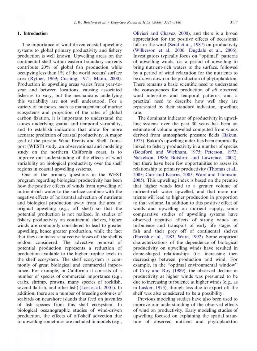
The MLC model represents biological productiv-ity in terms of the conveyor belt representationoften used to illustrate coastal upwelling (e.g.,

Fig. 1. A schematic view of the conceptual mixed-layer conveyor mode

flow across a continental shelf.

Wilkerson and Dugdale, 1987; Mann, 2000; Bots-ford et al., 2003) (Fig. 1). Parcels of water arebrought to the surface in response to wind, thentransported offshore, while the nutrients in each areprogressively converted to phytoplankton, thenzooplankton. The dynamics of conversion ofnutrients to phytoplankton, then to zooplankton,are represented by an NPZ model consisting ofthree nonlinear, coupled differential equations. Wemodel productivity in terms of nitrogen, which weassume to be the limiting nutrient, e.g., Kudela andDugdale (2000). Rate parameters for the singleforms of phytoplankton and zooplankton aresimilar to those in Botsford et al. (2003). Rateparameters are chosen to represent rates of increaseobserved in WEST studies (Wilkerson et al., 2006).We do not include the shift-up effect (Zimmermanet al., 1987) in the basic model, but assess theinfluence of that effect in the discussion. The initialconcentrations of nutrients (i.e. nitrate), phyto-plankton and zooplankton in upwelled water are17.5mM, 2mU and 0.5mM, respectively, based onobservations from WEST (Wilkerson et al., 2006).Values and units of all parameters for the NPZ

l portraying upwelling and shelf production as a two-dimensional


model are given in Table 1. Cross-shelf transport iscalculated from the rate of cross-shelf Ekmantransport and the depth of the mixed layer. Therates of shelf production for phytoplankton andzooplankton are taken to be the product of thevelocity at which parcels are brought to the surfaceand advected offshore and the cumulative uptakeper parcel up to the time that it leaves the shelf.Rate of production at time t is represented by

BðtÞ ¼ vðtÞF ½TðtÞ�, (1)

where v(t) is the cross-shelf velocity, F[s] thecumulative production after time s at the surface,T(t) the shelf transit time for a particle upwelled attime t.

The cross shelf velocity, v(t), in Ekman transportis

vðtÞ ¼dx

dt¼

ME

Dcst, (2a)

where ME is the Ekman mass transport and Dcst isthe depth of the layer being transported offshore,here assumed to be the depth of the surface mixed-layer depth (MLD). ME is related to alongshorewind stress by

ME ¼trf c

, (2b)

where r is the density of seawater, fc is the Coriolisparameter and the magnitude of the wind stress, t, is

t ¼ raCDV 2, (2c)

where V is wind speed and ra is density of air.Downwelling velocities are calculated, but down-

Table 1

Symbol descriptions, parameter values and units for the NPZ model

Symbol Symbol description

I Irradiance

Ks Half-saturation for P uptake of N

N Nutrient state variable

P Phytoplankton state variable

Rm Maximum ingestion rate of P�Z

Vm Maximum uptake rate of N�P

Z Zooplankton state variable

g Natural mortality rate of Z

kP Light extinction rate of P

kW Light extinction rate of seawater

m Natural mortality rate of P

L Grazing efficiency of Z on P

g Assimilated fraction of P ingested by Z

Z Regeneration rate of D–N

Parameter values are those of Franks and Walstad (1997).

welled volume is not subtracted when computingtotal upwelled volume. The wind-speed-dependentdrag coefficient CD was calculated as suggested byTrenbreth et al. (1990),

103CD ¼

0:49þ 0:065V for V410m s�1;

1:14 for 3ms�1pVp10m s�1;

0:62þ 1:5V�1 for Vo3m s�1:

8><>:

(2d)

Wind data for the model were taken from NDBCBuoy 46013 (hereafter referred to as buoy 13). Buoy13 is located 28 km offshore of Bodega Bay, CA at38.201N, 123.301W over the shelf at 125m waterdepth. To represent wind forcing over the appro-priate inertial time scale, the hourly data were low-pass filtered using PL64 which has a half-powerpoint of 38 h (Beardsley et al., 1985).

The surface MLD is calculated from the regres-sion relationship developed by Lentz (1992) for theCoastal Ocean Dynamics Experiment (CODE)study region, centered about 60 km north of theWEST study region:

MLDt ¼ 6:2þ 0:7ðhprtÞt�8. (3a)

MLDt is determined from hprt, lagged by 8 h. Thistime lag and the 38-h filter applied to the wind dataare assumed to provide a reasonable degree of offsetbetween the surface wind forcing, the evolution ofthe surface mixed layer and of the development ofoffshore Ekman transport. The parameter hprtdeveloped by Pollard et al. (1973), is based onwind-generated shear at the base of the surfacemixed layer and gives the wind-dependent scale of

Value Units

— mEm�2 s�1

1.0 mMN

— mMN

— mMN

0.5 day�1

1.0 day�1

— mMN

0.2 day�1

0.016 (mMP)�1m�1

0.06 m�1

0.1 day�1

0.2 (mMN)�1

0.7 Proportion

0.2 day�1


the depth of the surface mixed layer. The values ofthe coefficient A, the density of seawater, r, and thebuoyancy frequency, NI, are assumed to be con-stant.

hprt ¼ A

ffiffiffiffiffiffiffiffiffiffiffiffiffijtj

rf cNI

s. (3b)

The expressions for cumulative production, F,(Eq. (1)) differ for phytoplankton and zooplankton.They are based on a simple ecosystem model fornutrients, N, phytoplankton, P, and zooplankton,Z:

dN

dt¼ �

VmN

K s þNf ðIÞP, (4a)

dP

dt¼

VmN

K s þNf ðIÞP�mP� Rmð1� e�LPÞZ (4b)

and

dZ

dt¼ gRmð1� e�LPÞZ � gZ, (4c)

where the definition of variables is in Table 1. Thismodel represents new production. It is the modeldeveloped by Franks and Walstad (1997) with thefeedback paths from zooplankton and phytoplank-ton to nutrients removed. This was done to removethe inherent instability in the close coupling ofregenerated production when a parabolic mortalityrate, time delays or diffusion are not included(Edwards et al., 2000; Newberger et al., 2003;Botsford et al., 2003). The model was parameterizedto produce the magnitudes and time scales ofproductivity observed during WEST (Wilkerson etal., 2006).

The functions represented by F in Eq. (1) are thecumulative uptake of nutrients by phytoplankton,FP, and the cumulative consumption of phytoplank-ton by zooplankton, FZ. These are:

FPðTÞ ¼

Z T

0

VmN

K s þNf ðIÞPdt (5a)

and

FZðTÞ ¼

Z T

0

gRmð1� eLPÞZ dt, (5b)

where the integrands are the first terms in Eqs. (4b)and (4c), respectively, in the ecosystem models inEq. (3). FP(T) is the total gross phytoplanktonproduction in a parcel when it reaches the shelfedge, ignoring losses due to mortality and zoo-plankton consumption. FZ(T) is the total gross

zooplankton production in a parcel when it reachesthe shelf edge, ignoring zooplankton mortality.Both of these depend on the initial nutrientconcentration and light level. The influence of lightextinction by seawater and phytoplankton (Bannis-ter, 1974)

Iz ¼ I0e�ðkwþkPPÞz (6a)

is averaged over the assumed MLD. As such, themixed layer average light, including self-shading bythe phytoplankton, is computed from surface lightintensity (I0)

I ¼1

MLD

Z MLD

0

I0e�ðkwþkPPÞ, (6b)

which is

I ¼I0

MLDðkw þ kPPÞ1� e�ðkwþkPPÞMLD� �

, (6c)

and the light level influences phytoplankton growthaccording to

f ðIÞ ¼ 1� e�0:006I . (6d)

We assumed a MLD of 17m for the NPZ modelin spite of the t-dependent MLD used to calculateof cross-shelf velocity (described above). This wasan extension of our previous work (Botsford et al.,2003) in which a constant MLD of 17m was usedfor both. A MLD of 17m is typical for the WESTstudy region during upwelling favorable windconditions (Lentz, 1992; Dever et al., 2006). Wetested the sensitivity of our results to the assumptionof a constant MLD for the NPZ model bysimulating a more computationally intensive model.The results (described below) indicate little differ-ence between the assumed model and the morerealistic version. The value of T in Eq. (1) is the timeincrement required for a particle upwelled at time t

to cross a shelf of width W. It is given implicitly byZ tþT

t

vðtÞdt ¼W . (7)

3. Example of time series

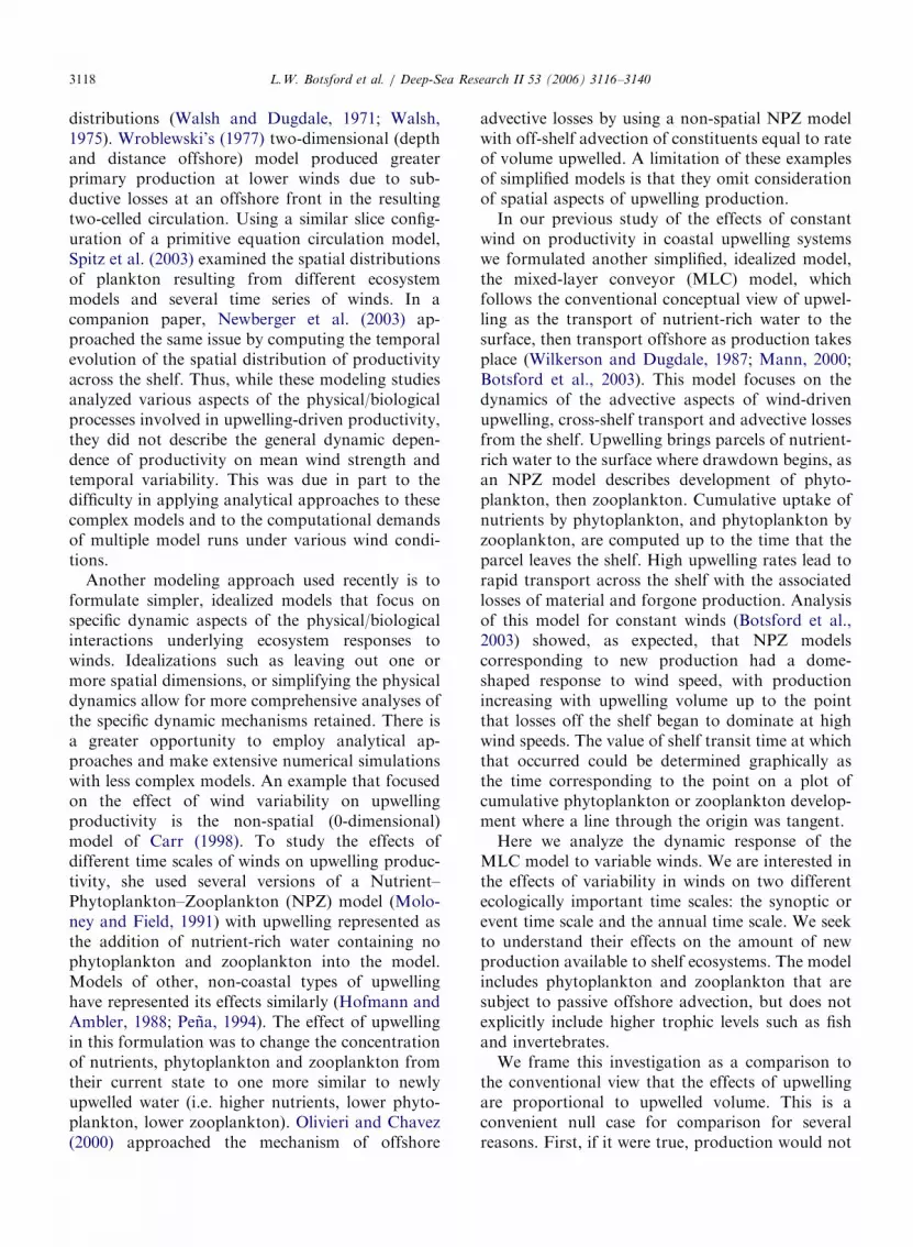
Plots of time series of the elements of Eq. (3)versus time for 2001 illustrate the nonlinearmechanisms involved in the production of phyto-plankton and zooplankton in the context ofthis model (Fig. 2). The cross-shelf velocity(Fig. 2A) reflects rather high upwelling during

ARTICLE IN PRESS

Fig. 2. MLC model example using NDBC Buoy 13 winds for 2001 and a shelf width of 35 km. (A) Cross-shelf velocity at each time

(negative values represent the offshore direction), (B) the time required for a parcel upwelled at time t to transit the shelf, (C) fraction of

maximum possible production of phytoplankton (green) and zooplankton (red) that would be produced in a parcel if it were upwelled at

time t, by the time it reached the edge of the shelf, (D) volume upwelled at each time t (UWindex, blue), and the resulting amount of

phytoplankton (Pindex, green) and zooplankton (Zindex, red) produced. Pindex and Zindex are the product of the fraction of maximum

production (Fig. 1C) and UWindex. The units of UWindex are 102 km.

L.W. Botsford et al. / Deep-Sea Research II 53 (2006) 3116–31403122

May, punctuated by occasional reversals. That isfollowed in early June by a period of moderateupwelling with no relaxations through June 25, afterwhich relaxations occur occasionally.

A salient feature of the plot of parcel-specific shelftransit times (Fig. 2B) is the jumps to high valuesfollowed by gradual declines. A substantial part ofthe production of both phytoplankton and zoo-plankton per upwelled parcel occurred in these

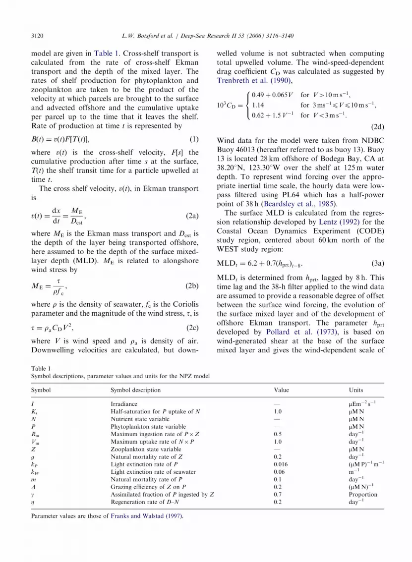
parcels with long transit times (Fig. 2C and D). Tounderstand why these occur, we expanded the timescale in Fig. 3A. The definition of T (Eq. (7)) as thetime taken for integrated velocity to move theparticle a distance W corresponds to examining theintegral of velocity to determine how long it takes toincrease by 35 km at each point (i.e. to move acrossthe shelf (Fig. 3B). In this plot, for each time, onemoves vertically a distance equal to the shelf width

ARTICLE IN PRESS

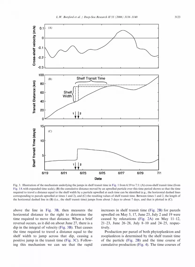
Fig. 3. Illustration of the mechanism underlying the jumps in shelf transit time in Fig. 1 from 6/19 to 7/1: (A) cross-shelf transit time (from

Fig. 1A with expanded time scale), (B) the cumulative distance moved by an upwelled particle over this time period shown so that the time

required to travel a distance equal to the shelf width by a particle upwelled at each time can be identified (e.g., the horizontal dashed lines

corresponding to parcels upwelled at times 1 and 2), and (C) the resulting values of shelf transit time. Between times 1 and 2, the length of

the horizontal dashed line in (B) (i.e., the shelf transit time) jumps from about 3 days to about 7 days, and that is plotted in (C).

L.W. Botsford et al. / Deep-Sea Research II 53 (2006) 3116–3140 3123

above the line in Fig. 3B, then measures thehorizontal distance to the right to determine thetime required to move that distance. When a briefreversal occurs, as it did on about June 27, there is adip in the integral of velocity (Fig. 3B). That causesthe time required to travel a distance equal to theshelf width to jump across that dip, causing apositive jump in the transit time (Fig. 3C). Follow-ing this mechanism we can see that the rapid

increases in shelf transit time (Fig. 2B) for parcelsupwelled on May 5, 17, June 23, July 2 and 19 werecaused by relaxations (Fig. 2A) on May 11–12,21–23, June 26–28, July 8–10 and 24–25, respec-tively.

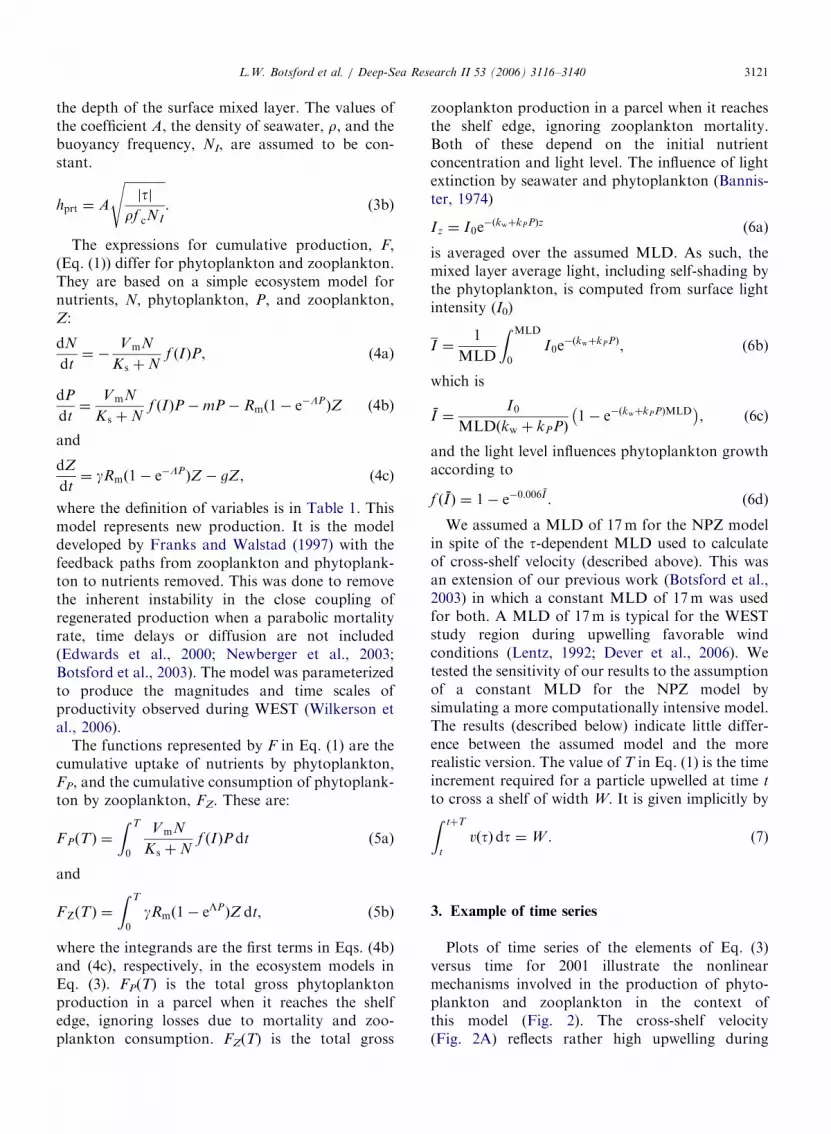
Production per parcel of both phytoplankton andzooplankton is determined by the shelf transit timeof the particle (Fig. 2B) and the time course ofcumulative production (Fig. 4). The time courses of

ARTICLE IN PRESS

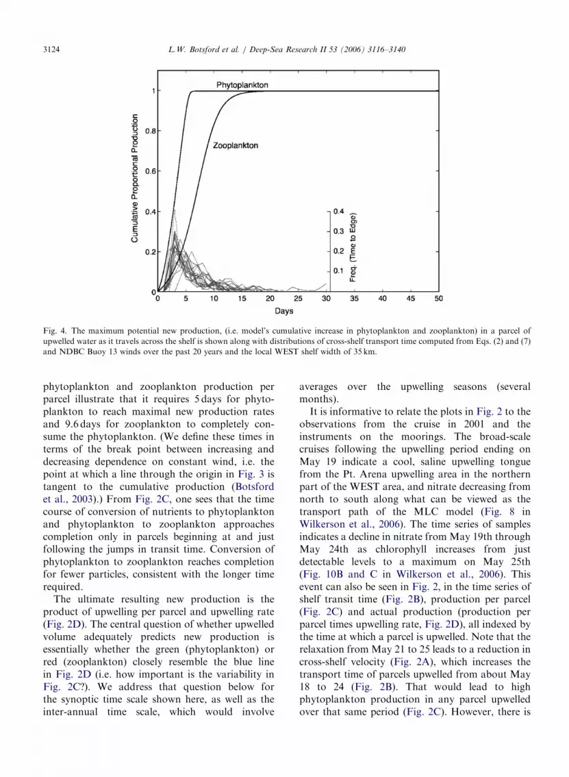
Fig. 4. The maximum potential new production, (i.e. model’s cumulative increase in phytoplankton and zooplankton) in a parcel of

upwelled water as it travels across the shelf is shown along with distributions of cross-shelf transport time computed from Eqs. (2) and (7)

and NDBC Buoy 13 winds over the past 20 years and the local WEST shelf width of 35 km.


phytoplankton and zooplankton production perparcel illustrate that it requires 5 days for phyto-plankton to reach maximal new production ratesand 9.6 days for zooplankton to completely con-sume the phytoplankton. (We define these times interms of the break point between increasing anddecreasing dependence on constant wind, i.e. thepoint at which a line through the origin in Fig. 3 istangent to the cumulative production (Botsfordet al., 2003).) From Fig. 2C, one sees that the timecourse of conversion of nutrients to phytoplanktonand phytoplankton to zooplankton approachescompletion only in parcels beginning at and justfollowing the jumps in transit time. Conversion ofphytoplankton to zooplankton reaches completionfor fewer particles, consistent with the longer timerequired.

The ultimate resulting new production is theproduct of upwelling per parcel and upwelling rate(Fig. 2D). The central question of whether upwelledvolume adequately predicts new production isessentially whether the green (phytoplankton) orred (zooplankton) closely resemble the blue linein Fig. 2D (i.e. how important is the variability inFig. 2C?). We address that question below forthe synoptic time scale shown here, as well as theinter-annual time scale, which would involve

averages over the upwelling seasons (severalmonths).

It is informative to relate the plots in Fig. 2 to theobservations from the cruise in 2001 and theinstruments on the moorings. The broad-scalecruises following the upwelling period ending onMay 19 indicate a cool, saline upwelling tonguefrom the Pt. Arena upwelling area in the northernpart of the WEST area, and nitrate decreasing fromnorth to south along what can be viewed as thetransport path of the MLC model (Fig. 8 inWilkerson et al., 2006). The time series of samplesindicates a decline in nitrate from May 19th throughMay 24th as chlorophyll increases from justdetectable levels to a maximum on May 25th(Fig. 10B and C in Wilkerson et al., 2006). Thisevent can also be seen in Fig. 2, in the time series ofshelf transit time (Fig. 2B), production per parcel(Fig. 2C) and actual production (production perparcel times upwelling rate, Fig. 2D), all indexed bythe time at which a parcel is upwelled. Note that therelaxation from May 21 to 25 leads to a reduction incross-shelf velocity (Fig. 2A), which increases thetransport time of parcels upwelled from about May18 to 24 (Fig. 2B). That would lead to highphytoplankton production in any parcel upwelledover that same period (Fig. 2C). However, there is


substantial upwelling only over the time periodfrom May 16 to 20, hence those parcels are the onlyones that realize that high phytoplankton produc-tion (Fig. 2D). The production in those parcels isobserved in the time series samples taken at the D2mooring from May 19 to 25 (Fig. 10 in Wilkerson etal., 2006), and also observed in the mooredinstruments (Fig. 1 in Kaplan and Largier, 2006).Note that for the dates shown, the pulse ofproductivity on May 19–25 was one of thedominant pulses in 2001, but was preceded by thepulse from parcels upwelled on May 10 (seen in Fig.1 of Kaplan and Largier, 2006).

4. Analysis and results

We are primarily interested in how characteristicsof the wind, such as the mean, the variance of thewind speed and the associated time scales ofvariability; affect biological productivity. For thisanalysis, we do not examine the effects of the hourlyscale time lags between wind speed and watervelocity, rather we assume that our approach tocalculation of MLD and Ekman transport minimizestheir effects on our results. This is reasonable giventhat observed MLD cross-shelf transports lag windforcing by 7h or less (Dever et al., 2006). We areinterested in variability in productivity on bothsynoptic (or upwelling event) and annual time scales.This variability will depend on the relative values ofvarious time scales, which we define here: Tcs is themean cross-shelf transit time, TP is the time tomaximum cumulative phytoplankton in a parcel(defined as the point on Fig. 4 where a line throughthe origin is tangent to the curve; Botsford et al.,2003), TZ is the time to maximum cumulativezooplankton in a parcel (defined the same way),and tw is the dominant time scale of variability in thewind. We analyze several different cases that illustratethe dependence of productivity on upwelling rate.

4.1. Production per parcel, F(T), held constant

From Eq. (1), if F[T(t)] is constant, shelfproductivity, B(t), will trivially be represented bycross-shelf velocity, which in this model is propor-tional to volume rate of upwelling.

4.1.1. Complete realization of potential new

production

Solutions to Eq. (3) indicate that after a particle isupwelled to the surface, conversion of nutrients to

phytoplankton and conversion of phytoplankton tozooplankton proceed to a constant level, themaximum potential primary and secondary newproduction (Fig. 4). The most obvious way that F

can be constant is if the mean transport time is longenough for complete realization of potential newproduction, and the standard deviation of transporttime is relatively low. If the transport times for allparcels are long enough that cumulative productionis always on the flat part of the curves in Fig. 4 (i.e.,Tcs4TP, Tcs4TZ), productivity will vary withvelocity only (Eq. (1)). In this case, the conventionalupwelling index (i.e. volume upwelled) will faithfullyrepresent the variability in productivity.

For the parameter values appropriate for theWEST study site, distributions of shelf transit timesfrom our model (Fig. 4) only occasionally allowed forcomplete realization of maximum potential primarynew production, and rarely allowed for completerealization of potential secondary new production (5and 9.6 days, respectively). Furthermore, box plots ofvariability from NDBC Buoy 13 winds within specificyears (Fig. 5) indicated that this held true for mostyears. Thus, the upwelling index may not representthe variability in shelf productivity at the WESTlocation, though it would at other locations withwider shelves and lower wind speeds.

4.1.2. Incomplete realization of potential new

production: short and long time scales

For situations with stronger upwelling winds andnarrower shelves such that this condition (i.e., T

long enough for cumulative shelf production to beon the flat part of the curves in Fig. 4) does nothold, it appears from Eq. (1) that F can still beconstant (and productivity will be proportional toupwelling index) if the shelf transit time, T, isconstant. To understand how T varies, we differ-entiate Eq. (7) to obtain,

dT

dt¼

vðtÞ

vðtþ TÞ� 1. (8)

Thus, changes in transit time, T, are determined byvalues of velocity separated by a time interval equalto the current value of T.

From this we can draw conclusions for severalcases. First, if the time scale of the winds is such thatthe time scales of variability in cross-shelf velocitiesare much greater than the mean transit time(tvbTcs), then v(t)/v(t+T) will always be near 1.0,and from Eq. (8), T will vary little. We also canconclude that if the time-scales of variability in the

ARTICLE IN PRESS

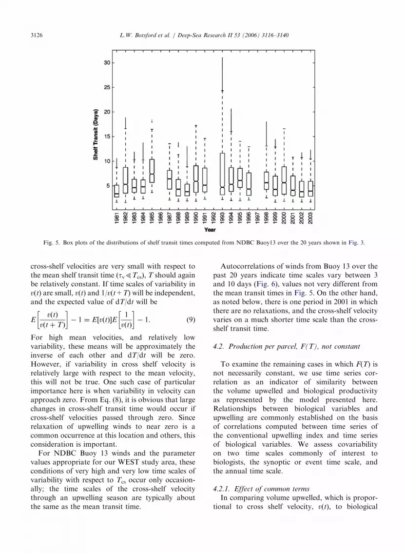
Fig. 5. Box plots of the distributions of shelf transit times computed from NDBC Buoy13 over the 20 years shown in Fig. 3.


cross-shelf velocities are very small with respect tothe mean shelf transit time (tv5Tcs), T should againbe relatively constant. If time scales of variability inv(t) are small, v(t) and 1/v(t+T) will be independent,and the expected value of dT/dt will be

EvðtÞ

vðtþ TÞ

� �� 1 ¼ E½vðtÞ�E

1

vðtÞ

� �� 1. (9)

For high mean velocities, and relatively lowvariability, these means will be approximately theinverse of each other and dT/dt will be zero.However, if variability in cross shelf velocity isrelatively large with respect to the mean velocity,this will not be true. One such case of particularimportance here is when variability in velocity canapproach zero. From Eq. (8), it is obvious that largechanges in cross-shelf transit time would occur ifcross-shelf velocities passed through zero. Sincerelaxation of upwelling winds to near zero is acommon occurrence at this location and others, thisconsideration is important.

For NDBC Buoy 13 winds and the parametervalues appropriate for our WEST study area, theseconditions of very high and very low time scales ofvariability with respect to Tcs occur only occasion-ally; the time scales of the cross-shelf velocitythrough an upwelling season are typically aboutthe same as the mean transit time.

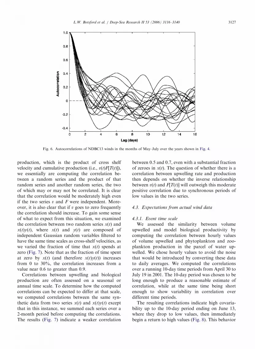
Autocorrelations of winds from Buoy 13 over thepast 20 years indicate time scales vary between 3and 10 days (Fig. 6), values not very different fromthe mean transit times in Fig. 5. On the other hand,as noted below, there is one period in 2001 in whichthere are no relaxations, and the cross-shelf velocityvaries on a much shorter time scale than the cross-shelf transit time.

4.2. Production per parcel, F(T), not constant

To examine the remaining cases in which F(T) isnot necessarily constant, we use time series cor-relation as an indicator of similarity betweenthe volume upwelled and biological productivityas represented by the model presented here.Relationships between biological variables andupwelling are commonly established on the basisof correlations computed between time series ofthe conventional upwelling index and time seriesof biological variables. We assess covariabilityon two time scales commonly of interest tobiologists, the synoptic or event time scale, andthe annual time scale.

4.2.1. Effect of common terms

In comparing volume upwelled, which is propor-tional to cross shelf velocity, v(t), to biological

ARTICLE IN PRESS

Fig. 6. Autocorrelations of NDBC13 winds in the months of May–July over the years shown in Fig. 4.


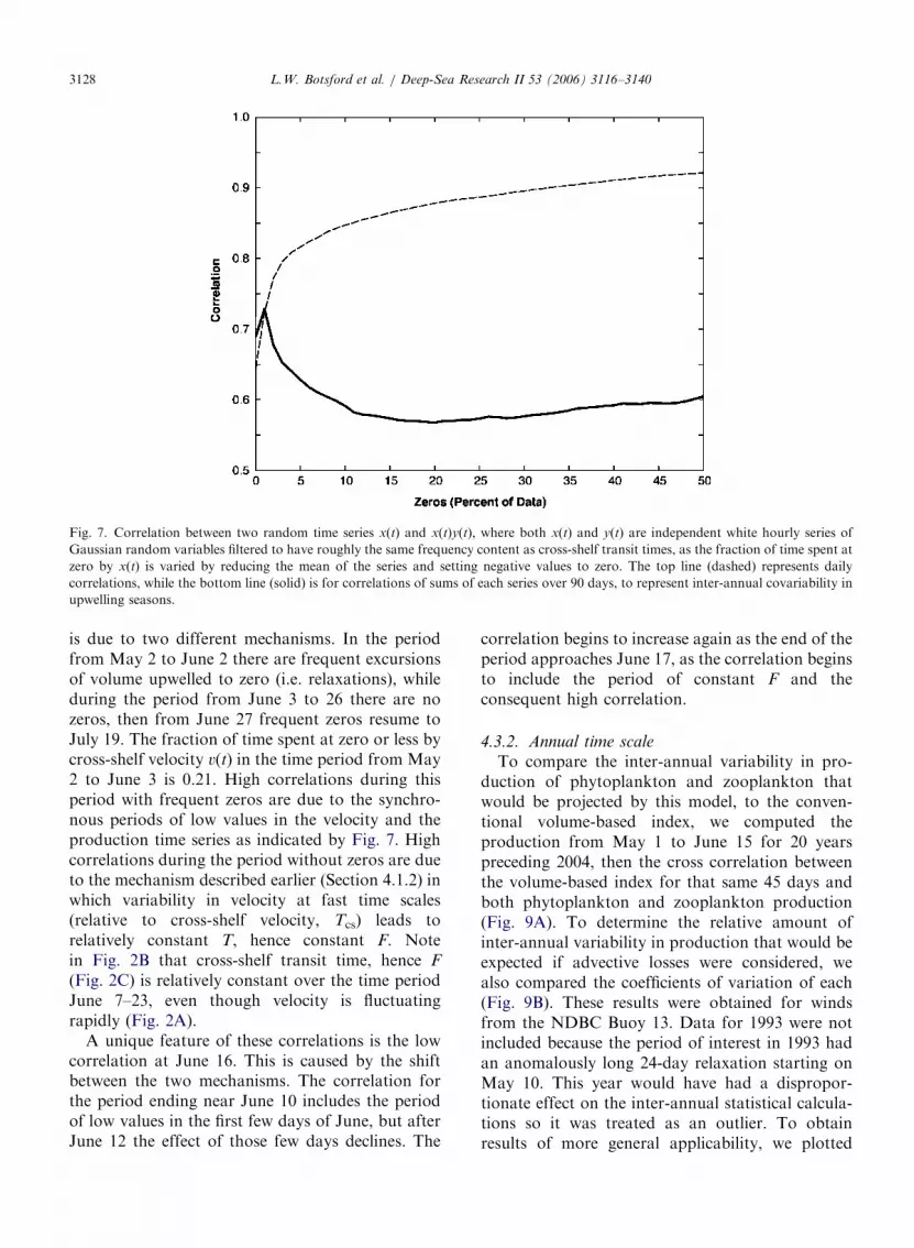
production, which is the product of cross shelfvelocity and cumulative production (i.e., v(t)F[T(t)]),we essentially are computing the correlation be-tween a random series and the product of thatrandom series and another random series, the twoof which may or may not be correlated. It is clearthat the correlation would be moderately high evenif the two series v and F were independent. More-over, it is also clear that if v goes to zero frequentlythe correlation should increase. To gain some senseof what to expect from this situation, we examinedthe correlation between two random series x(t) andx(t)y(t), where x(t) and y(t) are composed ofindependent Gaussian random variables filtered tohave the same time scales as cross-shelf velocities, aswe varied the fraction of time that x(t) spends atzero (Fig. 7). Note that as the fraction of time spentat zero by x(t) (and therefore x(t)y(t)) increasesfrom 0 to 30%, the correlation increases from avalue near 0.6 to greater than 0.9.

Correlations between upwelling and biologicalproduction are often assessed on a seasonal orannual time scale. To determine how the computedcorrelations can be expected to differ at that scale,we computed correlations between the same syn-thetic data from two series x(t) and x(t)y(t) exceptthat in this instance, we summed each series over a2-month period before computing the correlations.The results (Fig. 7) indicate a weaker correlation

between 0.5 and 0.7, even with a substantial fractionof zeroes in x(t). The question of whether there is acorrelation between upwelling rate and productionthen depends on whether the inverse relationshipbetween v(t) and F[T(t)] will outweigh this moderatepositive correlation due to synchronous periods oflow values in the two series.

4.3. Expectations from actual wind data

4.3.1. Event time scale

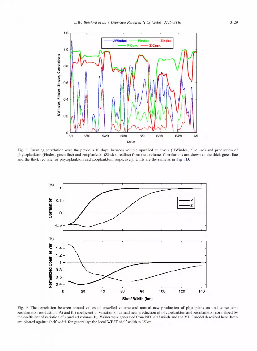
We assessed the similarity between volumeupwelled and model biological productivity bycomputing the correlation between hourly valuesof volume upwelled and phytoplankton and zoo-plankton production in the parcel of water up-welled. We chose hourly values to avoid the noisethat would be introduced by converting these datato daily averages. We computed the correlationsover a running 10-day time periods from April 30 toJuly 19 in 2001. The 10-day period was chosen to belong enough to produce a reasonable estimate ofcorrelation, while at the same time being shortenough to show variability in correlation overdifferent time periods.

The resulting correlations indicate high covaria-bility up to the 10-day period ending on June 13,where they drop to low values, then immediatelybegin a return to high values (Fig. 8). This behavior

ARTICLE IN PRESS

Fig. 7. Correlation between two random time series x(t) and x(t)y(t), where both x(t) and y(t) are independent white hourly series of

Gaussian random variables filtered to have roughly the same frequency content as cross-shelf transit times, as the fraction of time spent at

zero by x(t) is varied by reducing the mean of the series and setting negative values to zero. The top line (dashed) represents daily

correlations, while the bottom line (solid) is for correlations of sums of each series over 90 days, to represent inter-annual covariability in

upwelling seasons.


is due to two different mechanisms. In the periodfrom May 2 to June 2 there are frequent excursionsof volume upwelled to zero (i.e. relaxations), whileduring the period from June 3 to 26 there are nozeros, then from June 27 frequent zeros resume toJuly 19. The fraction of time spent at zero or less bycross-shelf velocity v(t) in the time period from May2 to June 3 is 0.21. High correlations during thisperiod with frequent zeros are due to the synchro-nous periods of low values in the velocity and theproduction time series as indicated by Fig. 7. Highcorrelations during the period without zeros are dueto the mechanism described earlier (Section 4.1.2) inwhich variability in velocity at fast time scales(relative to cross-shelf velocity, Tcs) leads torelatively constant T, hence constant F. Notein Fig. 2B that cross-shelf transit time, hence F

(Fig. 2C) is relatively constant over the time periodJune 7–23, even though velocity is fluctuatingrapidly (Fig. 2A).

A unique feature of these correlations is the lowcorrelation at June 16. This is caused by the shiftbetween the two mechanisms. The correlation forthe period ending near June 10 includes the periodof low values in the first few days of June, but afterJune 12 the effect of those few days declines. The

correlation begins to increase again as the end of theperiod approaches June 17, as the correlation beginsto include the period of constant F and theconsequent high correlation.

4.3.2. Annual time scale

To compare the inter-annual variability in pro-duction of phytoplankton and zooplankton thatwould be projected by this model, to the conven-tional volume-based index, we computed theproduction from May 1 to June 15 for 20 yearspreceding 2004, then the cross correlation betweenthe volume-based index for that same 45 days andboth phytoplankton and zooplankton production(Fig. 9A). To determine the relative amount ofinter-annual variability in production that would beexpected if advective losses were considered, wealso compared the coefficients of variation of each(Fig. 9B). These results were obtained for windsfrom the NDBC Buoy 13. Data for 1993 were notincluded because the period of interest in 1993 hadan anomalously long 24-day relaxation starting onMay 10. This year would have had a dispropor-tionate effect on the inter-annual statistical calcula-tions so it was treated as an outlier. To obtainresults of more general applicability, we plotted

ARTICLE IN PRESS

Fig. 8. Running correlation over the previous 10 days, between volume upwelled at time t (UWindex, blue line) and production of

phytoplankton (Pindex, green line) and zooplankton (Zindex, redline) from that volume. Correlations are shown as the thick green line

and the thick red line for phytoplankton and zooplankton, respectively. Units are the same as in Fig. 1D.

Fig. 9. The correlation between annual values of upwelled volume and annual new production of phytoplankton and consequent

zooplankton production (A) and the coefficient of variation of annual new production of phytoplankton and zooplankton normalized by

the coefficient of variation of upwelled volume (B). Values were generated from NDBC13 winds and the MLC model described here. Both

are plotted against shelf width for generality; the local WEST shelf width is 35 km.



both of these over a range of shelf widths possible inupwelling regions (specific to latitudes 38.21N or Sbecause of the Coriolis parameter in Eq. (3b)).

Biological production would be highly correlatedwith upwelling only for shelf widths of 50 km andgreater for phytoplankton, and approximately100 km and greater for zooplankton (Fig. 9A). Fornarrower widths, correlations decrease and becomenegative reaching values near �0.5. The amount ofvariability in annual shelf production due to wind-induced coastal upwelling also would vary withshelf width (as well as latitude and mean winds). Asshelf width narrows, the coefficient of variation(CV) of phytoplankton production declines frombeing the same as the CV of upwelling to 40–60percent over the range plotted (Fig. 9B). The CV ofzooplankton production also declines from beingthe same as the CV of upwelling as the shelf widthdeclines from high values (not shown), and thenincreases beginning at a shelf width of about 60 km.However, from Fig. 9A, the increase occurs over

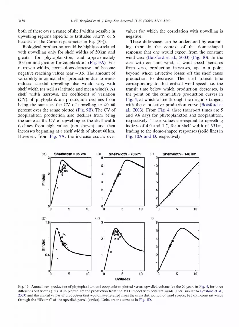
Fig. 10. Annual new production of phytoplankton and zooplankton pl

different shelf widths (x’s). Also plotted are the production from the M

2003) and the annual values of production that would have resulted fro

through the ‘‘lifetime’’ of the upwelled parcel (circles). Units are the sa

values for which the correlation with upwelling isnegative.

These differences can be understood by examin-ing them in the context of the dome-shapedresponse that one would expect from the constantwind case (Botsford et al., 2003) (Fig. 10). In thecase with constant wind, as wind speed increasesfrom zero, production increases, up to a pointbeyond which advective losses off the shelf causeproduction to decrease. The shelf transit timecorresponding to that critical wind speed, i.e. thetransit time below which production decreases, isthe point on the cumulative production curves inFig. 4, at which a line through the origin is tangentwith the cumulative production curve (Botsford etal., 2003). From Fig. 4, these transport times are 5and 9.6 days for phytoplankton and zooplankton,respectively. These values correspond to upwellingindices of 4.0 and 1.7, for a shelf width of 35 km,leading to the dome-shaped responses (solid line) inFig. 10A and D, respectively.

otted versus upwelled volume for the 20 years in Fig. 4, for three

LC model with constant winds (lines, similar to Botsford et al.,

m the same distribution of wind speeds, but with constant winds

me as in Fig. 1D.


The values of annual phytoplankton productionare the same as those for the constant wind case fora shelf width of 140 km, indicating that this width isadequate for complete realization of potential newproduction (Fig. 10C). As the shelf width becomesnarrower (Fig. 10B and A), annual phytoplanktonproduction falls below the values produced underconstant winds. Annual zooplankton productionfor a shelf width of 140 km (Fig. 10F) falls to the leftof the peak for the constant wind case and justbelow the constant wind values. For narrowershelves, values are below the peak (Fig. 10E) andto the right of the peak and greater than theconstant wind values (Fig. 10D).

The differences between the responses to constantand variable winds can be understood usingJensen’s inequality as a heuristic guide (for anotherbiological example, see Chesson, 1985). Accordingto Jensen’s inequality, if the response (productivity)to the input (winds) is either concave up or down(fixed sign of the second derivative of the function)over the range of non-time-varying inputs, then theresult of increasing variability while holding themean constant would be to increase or decrease(respectively) the mean of the response. This occursbecause points resulting from varying the indepen-dent variable about a point on a curved line willtake on values either above or below the tangent atthe mean value.

We can explain the differences between values ofannual production from constant wind and actualvariable winds by considering the distribution ofwinds, therefore transit times, within years and theconsequent cumulative production (Fig. 4), Fora wide shelf and short time scale of productivity(Fig. 10C), shelf transit times are always greaterthan 5 days so that production per parcel is constant(Fig. 4); hence production is proportional toupwelling velocity. As the shelf becomes narrower(Fig. 10B), some transit times within years will beless than 5 days, and production per parcel will beless than the maximum value. Values of upwellingindex corresponding to the transit times will rangefrom zero to values above the seasonal means orupwelling index at which each point in Fig. 10B isplotted; hence values of production for those pointswill be less than the value for constant winds, eventhough the mean value of upwelling index is in therange of increasing production for constant winds.This means that the points in Fig. 10B can lie belowthe line corresponding to constant winds, butcannot lie above the increasing part of that line.

As shelf width becomes shorter still (Fig. 10A), moretransit times will be less than 5 days. However,because the values of transit times in any specific yearinclude values corresponding to values of upwellingindex to the left of their mean, the points on Fig. 10Acan lie above the descending part of the curve fromconstant winds. The trend of increasingly shortertimes for production relative to the time required formaximal production, with constant winds can befollowed by turning to Fig. 10E, where the cloud ofpoints is roughly at the same point relative to thepeak. The cloud of points continues to the right inFig. 10D, but variability in production increases, inpart because of an increasing slope reflected in theconstant wind line, but also because of the decreasingtime over which randomly varying velocity is summedto reach the edge of the shelf.

4.4. Sensitivity to assumptions

To examine the sensitivity of our results to therate parameter for phytoplankton production (Vm),we computed time series of production per parcelfor values of times required for complete uptake(TP) ranging from 2 to 10 days (Fig. 11). As the timerequired for complete uptake decreased, the produc-tion per particle increased. Over most of this range,temporal patterns were quite similar to each other,with each result being a multiple of the others.However, as the rates approached values of 2 days,the amount of time for which phytoplanktonproduction per upwelled parcel was a maximumdominated the time series, and they were not similarto the others. For the values of rate parameterscorresponding to 4 days and greater, it appears thatthe results obtained here regarding the temporalcorrelation between upwelling rate and productionwould hold, based on the similarity in temporalpattern. For shorter uptake times, as the fraction ofparcels for which uptake is complete increased to1.0, the dependence of production on upwelling rateat inter-annual time scales (Fig. 10) would tend tofollow the ascending part of the relationship forconstant winds, even for a 35 km shelf.

To examine the sensitivity of our results to the useof a simplified surface-mixed layer representation inthe MLC, particularly the use of a constant MLD of17m for the biological model and a t-dependentMLD for the physical model, we simulated a fullyt-dependent MLD in which light was explicitlycalculated over 30 layers of 1m depth rather thanbeing averaged. The results of this model are shown

ARTICLE IN PRESS

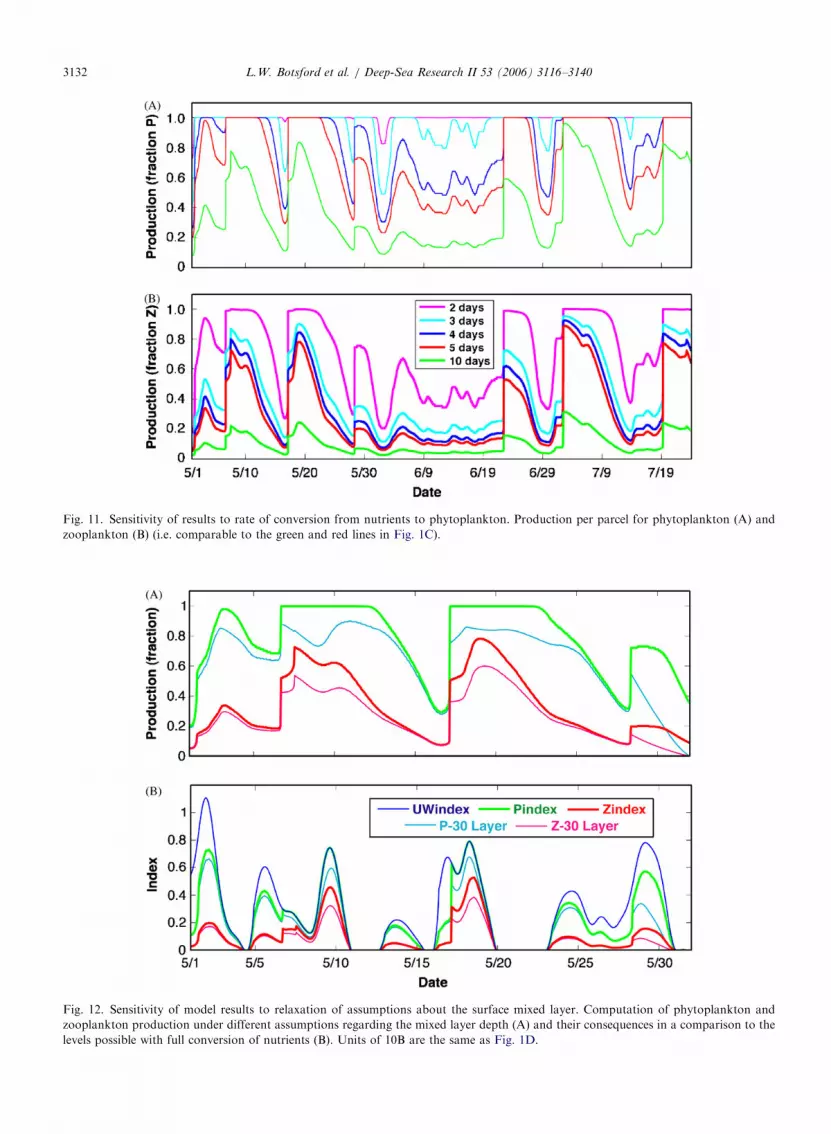
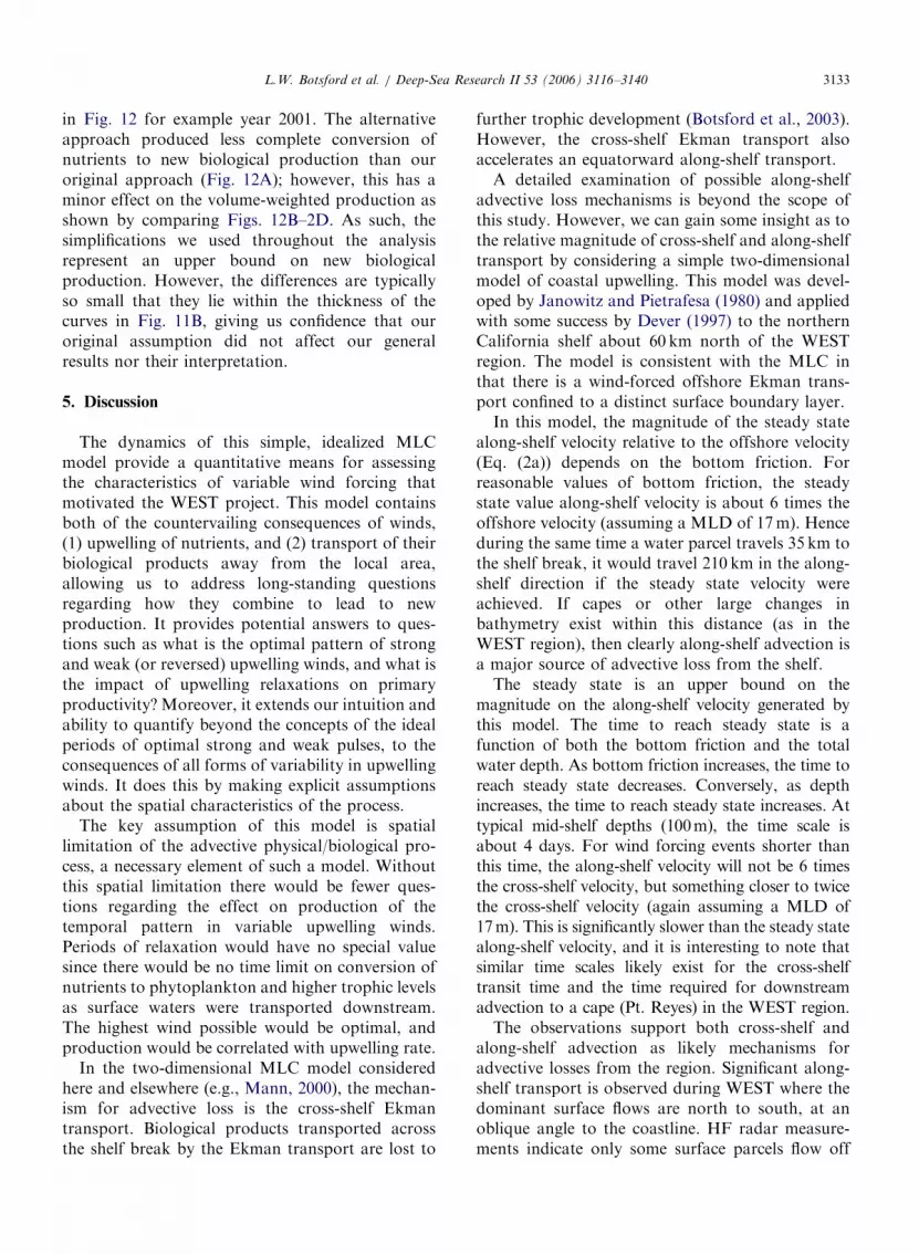
Fig. 11. Sensitivity of results to rate of conversion from nutrients to phytoplankton. Production per parcel for phytoplankton (A) and

zooplankton (B) (i.e. comparable to the green and red lines in Fig. 1C).

Fig. 12. Sensitivity of model results to relaxation of assumptions about the surface mixed layer. Computation of phytoplankton and

zooplankton production under different assumptions regarding the mixed layer depth (A) and their consequences in a comparison to the

levels possible with full conversion of nutrients (B). Units of 10B are the same as Fig. 1D.



in Fig. 12 for example year 2001. The alternativeapproach produced less complete conversion ofnutrients to new biological production than ouroriginal approach (Fig. 12A); however, this has aminor effect on the volume-weighted production asshown by comparing Figs. 12B–2D. As such, thesimplifications we used throughout the analysisrepresent an upper bound on new biologicalproduction. However, the differences are typicallyso small that they lie within the thickness of thecurves in Fig. 11B, giving us confidence that ouroriginal assumption did not affect our generalresults nor their interpretation.

5. Discussion

The dynamics of this simple, idealized MLCmodel provide a quantitative means for assessingthe characteristics of variable wind forcing thatmotivated the WEST project. This model containsboth of the countervailing consequences of winds,(1) upwelling of nutrients, and (2) transport of theirbiological products away from the local area,allowing us to address long-standing questionsregarding how they combine to lead to newproduction. It provides potential answers to ques-tions such as what is the optimal pattern of strongand weak (or reversed) upwelling winds, and what isthe impact of upwelling relaxations on primaryproductivity? Moreover, it extends our intuition andability to quantify beyond the concepts of the idealperiods of optimal strong and weak pulses, to theconsequences of all forms of variability in upwellingwinds. It does this by making explicit assumptionsabout the spatial characteristics of the process.

The key assumption of this model is spatiallimitation of the advective physical/biological pro-cess, a necessary element of such a model. Withoutthis spatial limitation there would be fewer ques-tions regarding the effect on production of thetemporal pattern in variable upwelling winds.Periods of relaxation would have no special valuesince there would be no time limit on conversion ofnutrients to phytoplankton and higher trophic levelsas surface waters were transported downstream.The highest wind possible would be optimal, andproduction would be correlated with upwelling rate.

In the two-dimensional MLC model consideredhere and elsewhere (e.g., Mann, 2000), the mechan-ism for advective loss is the cross-shelf Ekmantransport. Biological products transported acrossthe shelf break by the Ekman transport are lost to

further trophic development (Botsford et al., 2003).However, the cross-shelf Ekman transport alsoaccelerates an equatorward along-shelf transport.

A detailed examination of possible along-shelfadvective loss mechanisms is beyond the scope ofthis study. However, we can gain some insight as tothe relative magnitude of cross-shelf and along-shelftransport by considering a simple two-dimensionalmodel of coastal upwelling. This model was devel-oped by Janowitz and Pietrafesa (1980) and appliedwith some success by Dever (1997) to the northernCalifornia shelf about 60 km north of the WESTregion. The model is consistent with the MLC inthat there is a wind-forced offshore Ekman trans-port confined to a distinct surface boundary layer.

In this model, the magnitude of the steady statealong-shelf velocity relative to the offshore velocity(Eq. (2a)) depends on the bottom friction. Forreasonable values of bottom friction, the steadystate value along-shelf velocity is about 6 times theoffshore velocity (assuming a MLD of 17m). Henceduring the same time a water parcel travels 35 km tothe shelf break, it would travel 210 km in the along-shelf direction if the steady state velocity wereachieved. If capes or other large changes inbathymetry exist within this distance (as in theWEST region), then clearly along-shelf advection isa major source of advective loss from the shelf.

The steady state is an upper bound on themagnitude on the along-shelf velocity generated bythis model. The time to reach steady state is afunction of both the bottom friction and the totalwater depth. As bottom friction increases, the time toreach steady state decreases. Conversely, as depthincreases, the time to reach steady state increases. Attypical mid-shelf depths (100m), the time scale isabout 4 days. For wind forcing events shorter thanthis time, the along-shelf velocity will not be 6 timesthe cross-shelf velocity, but something closer to twicethe cross-shelf velocity (again assuming a MLD of17m). This is significantly slower than the steady statealong-shelf velocity, and it is interesting to note thatsimilar time scales likely exist for the cross-shelftransit time and the time required for downstreamadvection to a cape (Pt. Reyes) in the WEST region.

The observations support both cross-shelf andalong-shelf advection as likely mechanisms foradvective losses from the region. Significant along-shelf transport is observed during WEST where thedominant surface flows are north to south, at anoblique angle to the coastline. HF radar measure-ments indicate only some surface parcels flow off


the shelfbreak in this region, with the remaindertransported to the south (Kaplan and Largier,2006). Production could be lost to local highertrophic levels downstream at capes where along-shelf transport can leave the coast in upwellingfilaments (e.g., Strub et al., 1991; referred to in Wareand Thomson, 2005) or where along-shelf upwellingjets are subducted beneath less dense coastal waters(Collins et al., 2003). Thus downstream along-shelftransport constitutes an important alternative ad-vective loss mechanism.

Our model results presented depend on accuraterepresentation of the effects of wind on the MLD.WEST observations indicate calculation of theMLD from Eq. (3) is adequate for our purposes.Dever et al. (2006), estimate surface boundary layerdepths for the WEST region and calculate Ekmantransport (relative to the interior flow). They findsurface MLDs ranging from 0 (during wind relaxa-tion events) to 40m or more (during strongupwelling events). The MLD used here is qualita-tively consistent with their results. Dever et al.(2006) also calculate observed surface boundarylayer transports and find that the observed offshoresurface boundary layer transport is well correlatedwith, and similar in magnitude to, the Ekmantransport estimated from wind stress. This finding iswell supported by historical results and is commonto several coastal upwelling regions (Lentz, 1992).

Our understanding of the effects of time-varyingwinds on shelf production can be summarized as thecombination of two effects: (1) the inverse effect oflosses with high winds and (2) the effect ofsynchronous periods of low values in the time seriesof upwelling rate and production. These combineand sometimes work at cross-purposes for differentlevels of average wind and different time scales ofinterest.

The inverse effect of losses with high winds can beseen in the dome-shaped relationship that resultedfor new production only in our earlier investigationof the effects of constant winds (i.e. the lines inFig. 10). The shape of that relationship is deter-mined by the spatial limitation, which in conjunc-tion with wind speed, sets the dominant physicaltime scale, here referred to as the cross-shelf transittime (Tcs). The dominant physical time scale incomparison with the dominant biological timescales, the time to complete nutrient uptake byphytoplankton (TP), and the time to maximalzooplanton population development (TZ) determinethe dynamic behavior of production in response to

winds. When the dominant biological time scaleexceeds the dominant physical time scale, increasingwind strength shifts from having a positive effect toa negative effect in a way that is transparent forconstant winds.

The effect of synchronous periods of low values inthe wind and the production series (due to windrelaxations) arises when temporal variability in thewind is introduced. It has two important character-istics: (1) it has a positive effect on the correlationbetween upwelling rate and production, in spite ofthe fact that relaxation (low wind) represents aninverse effect on production (high production), and(2) it depends on the time scale of observation, beingstronger at the synoptic (event) scale, but stillhaving an effect at the inter-annual scale. The lattercharacteristic occurs because inter-annual variabil-ity involves averaging upwelling rate and produc-tion over a season, thus reducing the presence of theshorter time scale.

In addition to these major effects, we also sawthat when temporal variability is added, windvariability on time scales (tw) either much shorterthan or much longer than the dominant physicaltime scale, Tcs can lead to a positive correlationbetween upwelling rate and production (Section4.1.2).

The scientific implications of these results dependon the time scale of interest to investigators. Onsynoptic (event) time scales, prediction of produc-tion from winds would be of interest to investigatorsof event scale effects of productivity on filter-feedinginvertebrates in the inter-tidal zone. Their investiga-tions address issues such as the trophic organizationof intertidal communities (Menge, 2000) and thegeographic variability in abundance and growthrate that could determine species distribution andabundance. They compare growth to synoptic scalevariability in upwelling (e.g., Sanford and Menge,2001) and compare community interactions amongareas of the California Current that are differen-tiated on the basis of the time scales of variability intheir upwelling winds (Menge et al., 2004). Ourresults on synoptic time scales are also relevant tofeeding and growth of nearshore rockfish, whosefeeding behavior is influenced synoptic scale varia-bility in upwelling (Hobson and Chess, 1988).

Strictly speaking our MLC model would notapply shoreward of the depths over which surfaceEkman transport divergence (i.e. upwelling) oc-curred. For the spatially uniform wind forcingconsistent with our model, Ekman transport


divergence occurs in depths shallow enough suchthat there is a direct transfer of the turbulentmomentum flux from the surface to the bottomboundary layer. The spatial extent of this region,often called the inner shelf, depends strongly on theinterior stratification. The exact spatial extent of theinner shelf is not well known. When stratificationexists, the inner shelf can be as shallow as 15–30mdepth (e.g., Lentz, 2001; Kirincich et al., 2005). Forthe WEST observations, available evidence (Deveret al., 2006) indicates that the 40-m mooring isusually outside the inner shelf for spring 2001. Thatis, the inner shelf boundary is somewhere between40m and the coast, a distance of 1.5 km.

In spite of the fact that the inter-tidal areas areshoreward of these depths, the clear examples ofobserved effects of synoptic scale variability oninter- and sub-tidal ecology mentioned aboveindicates the variation in productivity described inour model does affect these areas. Also, since thearea of interest for intertidal studies is the nearshore, one would expect mechanisms involvinglosses due to advection out of the area of interestto be particularly relevant. Our results indicate that,in spite of a negative relationship between produc-tivity per parcel upwelled and wind stress, there islikely to be a strong correlation between volumeupwelled and productivity. The basis of thatcorrelation is the presence of synchronous periodsof low values in volume upwelled and productivity(volume upwelled times productivity per unitvolume).

Taken at face value, this suggests that thestandard upwelling index remains a useful indicatorof productivity, and it can continue to be used todetect the presence and absence of such a relation-ship. However, this result also indicates that therecould be a negative effect of wind on productivitypresent, yet it would be occluded by the positiveeffect of the synchronous periods of low values inwind and production. This latter considerationsuggests that attempting to detect both effectsthrough use of a model such as the MLC wouldlead to a more comprehensive description withgreater fidelity and usefulness. For example, findinga positive correlation between upwelling andproduction could lead to the conclusion that therewas not an inverse effect of strong winds onproductivity, even when it was present.

Turning to the annual time scale where windeffects are commonly summed or averaged over theupwelling period of several months, then compared

with annual productivity, the effect of the synchro-nous periods of low values on signal detection isreduced. For example, the correlation between x(t)and x(t)y(t), where x(t) and y(t) were independent,was near 0.9 for the synoptic time scale, but for theannual time scale dropped to near 0.5 (Fig. 7). Inspite of the fact that the effect of synchronousperiods of low values on the correlation betweenupwelling rate and production is real, in attemptingto detect the relationship between upwelling windsand production that one would see with constantwinds, it introduces a bias in correlation in thedirection of a positive relationship. This effect isevident, for example, in the lack of symmetry inFig. 9A. For broad shelves, when the productivityhas a positive dependence on upwelled volume(Fig. 10C), a correlation of 1.0 is possible, however,for narrow shelves, where productivity has a negativedependence on upwelled volume (Fig. 10D), themaximum (negative) correlation is �0.5 (Fig. 9A).Thus, results at the annual scale also suggest a modelthat includes both the positive and negative aspectsof the production process be used to investigate themechanism(s) by which upwelling and productionare related. Another possible alternative, that weadjust for the positive bias that appears to be 0.5both for artificially generated series (Fig. 7) and forreal wind series (Fig. 9A), would be risky since themagnitude of the bias depends on the details of thedistribution of wind strengths and the length of theperiod over which winds are summed or averages.Longer periods would lead to less bias, but it wouldbe difficult to predict the bias on the basis of a singlerealization of the process.

The use of an MLC model in detection andprediction of the effects of wind variability onbiological production apparently would improvethose efforts, yet would not place a great additionalburden on them. As seen in Eq. (1) it requires onlyadding an expression of the potential productivityper parcel. The upwelling velocity can be taken fromexisting calculations of the upwelling index orcomputed directly from buoy winds, as was donehere. Calculation of potential productivity perparcel for new phytoplankton production wouldnot require the full biological model used here, butrather only a means for constructing a cumulativephytoplankton production curve such as that inFig. 4. The most important aspect of that curve isthat it have the correct time scale. Based onobservations in a number of areas that time scaleis in the range of 3–7 days (Dugdale et al., 2006).


The next step, choosing a spatial scale, is somewhatspeculative, as it requires settling on a physicalmechanism. The goal would be to characterize thedominant, upwelling-driven flow in the region ofinterest by choice of the spatial dimension of themodel. Because of the uncertainty in the appro-priate physical spatial scale and the biologicaltemporal scale, another possibility is to include ageneral dome-shaped relationship, and fit it to thestatistical characteristics of the data by appropriatechoice of parameter values.

The lack of a linear increase in production withupwelling velocity as described here may be in partresponsible for the lack of consistent relationshipsbetween annual upwelling indices and production athigher trophic levels. In the California Current,correlations between Bakun’s upwelling index andbiological indicators are sometimes found (Botsfordand Wickham, 1975; Nickelson, 1986; Botsford andLawrence, 2002), but just as often are not found.Notably, Nickelson’s (1986) correlation betweenupwelling index and coho salmon became negativeand statistically insignificant after the decadal scaleshift in ocean conditions in the mid-1970s (Pearcy,1997). Interpretation of the role of upwelling indetected biological responses is clouded by the factthat the upwelling index (which is computed fromatmospheric pressure observations) is highly corre-lated with other hydrographic indicators that varywith biological production in the CCS (i.e. sea leveland temperature) (Botsford and Lawrence, 2002).There is also a long-standing question as to whetherwind-induced coastal upwelling is the source ofnutrients in this system (Reid, 1962). Alongshoreadvection from the north was proposed as analternative based on a lack of correlation betweenzooplankton and upwelling (Chelton et al., 1982).However, Collins et al. (2003) recently reporteddirect observations of wind-driven upwelling as thesource. Other mechanisms, at least on longer,decadal time scales include the depth of the mixedlayer (McGowan et al., 2003). Our results here (i.e.Fig. 10D and E) indicate that even if wind-inducedcoastal upwelling were driving biological produc-tion, there could still be very little annual variabilityin new production, and that the consequentzooplankton production could be poorly or nega-tively correlated.

Several observations are consistent with thepredicted consequences of the MLC mechanism. Adome-shaped relationship between upwelling windsand meroplankton settlement was described in our

earlier analysis of the response of the MLC toconstant winds (Botsford et al., 2003). Another localexample is the comparison of growth rates ofjuvenile salmon between years of strong and weakupwelling. Growth rates of Chinook salmon in theGulf of the Farallones in 1998 and 1999 unexpect-edly showed little difference in growth (Botsford,2002; MacFarlane et al., 2002).

From a global, more spatial perspective, therange of cross-shelf velocities and shelf widths in thefour major coastal upwelling regions (Carr andKearns, 2003) indicate the mechanism studied herecould affect expectations regarding productivity.From satellite-derived chlorophyll estimates, Tho-mas et al. (2003) found that the latitudes ofmaximum chlorophyll a were generally the latitudesof greatest upwelling. From their examination of anumber of hydrographic variables, Carr and Kearns(2003) found that spatial and temporal variabilitywas due to the effect of large-scale circulation onsource waters, sometimes in conjunction with localwind forcing. Analyses such as these could benefitby considering the potential for advective losses offcontinental shelves, using calculations such as theMLC model. Indications that the timescales ofphytoplankton development are similar betweensystems (see Wilkerson et al., 2006; Dugdale et al.,2006) imply that the differences between systemsmay depend on differences in shelf widths, meanwinds, the time scale of wind variability and thefrequency of relaxations.

The potential global implications of the resultsobtained here can be understood in terms of therelationships between time scales by defining acharacteristic velocity for a location as the ratio ofthe shelf width (W) to the time scale of biologicalproduction (TP or TZ), then plotting productionfrom constant winds and variable winds withvelocity normalized by that characteristic velocity(Fig. 13). This essentially allows all of the plots inFig. 10 to be approximated in a single plot. Forweak wind and a low relative velocity, the ascendinglimb of the dome-shaped relationship is followedclosely, but as we depart from those conditions,production from variable winds is initially less thanthat predicted from constant winds, then at somepoint crosses the descending limb of the constantwind relationship and remains greater than theconstant wind relationship, declining more gradu-ally. A critical aspect of this general view is that thelocations of the ellipsoids representing variabilitydepend critically on the fact that as we increase the

ARTICLE IN PRESS

Fig. 13. A schematic view of how productivity varies with a

generalized velocity, normalized by dividing by a characteristic

velocity associated with the location. The characteristic velocity,

v*, is the shelf width divided by the time scale of biological

production.


average normalized velocity, the distribution ofwinds still contains zeroes (i.e. relaxations).

The MLC model runs presented here comparesclosely to observations, both in terms of biologicaland physical processes and the consequences for thedependence of productivity on wind speed andpattern. The biological parameters were chosen torepresent typical patterns of new production both inWEST and in other upwelling systems. The time tocomplete nutrient uptake by phytoplankton in theMLC is about 5 days (Fig. 4), which comparesfavorably with the duration of 6 days Fig. 11C inWilkerson et al. (2006) and is within the generallyregarded range of 3–7 days (Wilkerson et al., 2006).Sensitivity runs varying drawdown time (Fig. 11)indicate that the results obtained here regardingcorrelation with upwelling volume on various timescales should hold for all but the fastest times (2days). The dominant flows in WEST as seen in theHF radar and other data, involve upwelling andtransport of water offshore and out of the local areawith a spatial scale near 35 km. The time scales oftransport off the shelf and out of the local arearange from 2 to 6 days, and vary with the wind(Figs. 15 and 16 in Kaplan and Largier, 2006).Additional, more direct comparisons are planned.

Other models and observations show losses offthe shelf. A non-spatial version of the model ofFasham et al. (1990) parameterized for upwellingnear Monterey, 200 km to the south of the WESTsite, produced the result that slightly greater thanhalf of the primary production was exported, andthat result compared favorably with field values(Olivieri and Chavez, 2000). From Fig. 10A for the35-km shelf, projecting the linear part of the

phytoplankton production curve to higher upwel-ling values so that the offshore losses are ignoredshows that the values of production we obtain hereare just greater than half of the projected linearvalues at the mean upwelling value. From hydro-graphic observations near Monterey Bay in centralCalifornia, Collins et al. (2003) identified subduc-tion beneath the coastal jet as a potential mechan-ism for offshore loss at that location.

We have used an idealized model here raising thequestion of the effects of factors not directlyaccounted for. We explicitly evaluated the effectsof leaving the wind-driven variability in the MLDout of the production calculation. It affects the scaleof the production, but not the temporal pattern,which is the focus here. A similar comment can bemade regarding sinking; to a first approximation,the influence of sinking on rates of new productionare not likely to change with the time scale offorcing. We have not specifically addressed theconsequences of the shift-up phenomenon (Zimmer-man et al., 1987), but it is represented to somedegree our examination of the range of developmentrates. Another important effect not accounted for inour model is the tendency of diel vertical migrationof some zooplankton to lead to their greaterretention on than shelf than the passive particlesdepicted here (Batchelder et al., 2002). Lastly, theMLC model is not well suited for easy incorpora-tion of the recent WEST results involving upwellingdue to wind stress curl (Dorman et al., 2005), but tothe degree that the curl is correlated with themagnitude of wind stress (Dorman et al., 2005), theresults here would apply.

More complex models could be formulated toinclude these effects, but that would be at theexpense of run times and ease of analysis. Three-dimensional circulation models for the WESTlocation have been developed (Gan and Allen,2002a, b; Kuebel Cervantes and Allen, 2005), andthe latter includes Lagrangian tracers, a capabilitythat would be useful in the context of the topic here.A two-dimensional ‘‘slice’’ model (Spitz et al., 2003)and a model that advects NPZ models along acharacteristic line (Newberger et al., 2003) havebeen used to assess the cross-shelf spatial distribu-tion of biological material. An approach thatcompared the mechanisms and effects describedhere among models of varying complexity is areasonable way to pursue further investigation ofthe consequences identified in this simple, idealizedmodel. Such an approach could also explore some


of the mechanisms not accounted for here, such asdiel vertical migration of zooplankton.

6. Conclusions

Adding temporal variability in winds to an MLCmodel that appears to reflect the relationshipbetween observations of chlorophyll, wind, andsurface transport in the WEST program hasrevealed that high winds can have an inverse effecton new production. The common practice ofcomputing correlations between time series ofupwelled volume and biological variables is at-tempting to detect a biologically meaningful effectof upwelling, but the resulting covariability is due totwo mechanisms, (1) the effect of wind on produc-tion, and (2) the effect of synchronous periods oflow values. The former can tend to produce morenegative correlations, and the latter more positivecorrelations. The effects of time-varying winds andupwelling on biological production are in this sensevery different from conclusions we might reachviewing the process as merely a noisy version ofconstant upwelling. Accounting for the possibilityof an inverse relationship using a model similar tothe MLC may be useful in increasing our under-standing of variability in new production on bothsynoptic (event) and inter-annual time scales.

Acknowledgments

Funding was provided by the NSF Coastal OceanProcesses (CoOP) program (LWB, CAL and AHfunded by OCE-9910897) (EPD and JLL funded byOCE-9907884). This work benefited greatly fromdiscussions with our WEST colleagues, especiallyDick Dugdale, Frances Wilkerson, David Kaplan,and Raphe Kudela. We also thank the anonymousreviewers for their comments.

References

Bannister, T.T., 1974. A general theory of steady state

phytoplankton growth in a nutrient saturated mixed layer.

Limnology and Oceanography 19, 13–30.

Bakun, A., 1973. Coastal upwelling indices, west coast of North

America, 1946–1971. NOAA Technical report, NMFS SSRF-

671, 103pp.

Batchelder, H.P., Edwards, C.A., Powell, T.M., 2002. Individual-

based models of copepod populations I: coastal upwelling

regions: implications of physiologically and environmentally

influenced diel vertical migration on demographic success and

nearshore retention. Progress in Oceanography 53, 307–333.

Beardsley, R.C., Limeburner, R., Rosenfeld, L.K., 1985.

Introduction to the CODE-2 moored array and large-scale

data report. In: Limeburner, R. (Ed.), CODE-2: Moored

Array and Large-scale Data Report. WHOI Technical report,

WHOI-85-35, 234pp.

Botsford, L.W., 2002. Ocean influences on Central Valley

Salmon: the rest of the story. IEP Newsletter 15, 47–52.

Botsford, L.W., Wickham, D.E., 1975. Correlation of upwelling

index and Dungeness crab catch. US Fishery Bulletin 73 (4),

901–907.

Botsford, L.W., Lawrence, C.A., 2002. Patterns of co-variability

among California current Chinook salmon, Coho salmon,

Dungeness crab, and physical oceanographic conditions.

Progress in Oceanography 53, 283–305.

Botsford, L.W., Lawrence, C.A., Dever, E.P., Hastings, A.,

Largier, J., 2003. Wind strength and biological productivity in

upwelling systems: an idealized study. Fisheries Oceanogra-

phy 12, 245–259.

Carr, M.-E., 1998. A numerical study of the effect of periodic

nutrient supply on pathways of carbon in a coastal upwelling

regime. Journal of Plankton Research 20, 491–516.

Carr, M.-E., Kearns, E.J., 2003. Production regimes in four

Eastern boundary current systems. Deep-Sea Research II 50,

3199–3221.

Chelton, D.B., Bernal, P.A., McGowan, J.A., 1982. Large-scale

interannual physical and biological interaction in the Cali-

fornia Current. Journal of Marine Research 40, 1095–1125.

Chesson, P.L., 1985. Coexistence of competitors in spatially and

temporally varying environments: a look at the combined

effects of different sorts of variability. Theoretical Population

Biology 28, 263–287.

Collins, C.A., Pennington, J.T., Castro, C.G., Rago, T.A.,

Chavez, F.P., 2003. The California current system off

monterey, California: physical and biological coupling.

Deep-Sea Research II 50, 2389–2404.

Cury, P., Roy, C., 1989. Optimal environmental window and

pelagic fish recruitment success in upwelling areas. Canadian

Journal of Fisheries and Aquatic Sciences 46, 670–680.

Cushing, D.H., 1971. Upwelling and the production of fish.

Advances in Marine Biology 9, 255–334.

Dever, E.P., 1997. Wind-forced cross-shelf circulation on the

northern California shelf. Journal of Physical Oceanography

27, 1566–1580.

Dever, E.P., Dorman, C.E., Largier, J.L., 2006. Surface

boundary layer variability during spring and summer upwel-

ling. Deep-Sea Research II, accepted for publication.

Dorman, C.E., Dever, E.P., Largier, J., Koracin, D., 2005. Buoy

measured wind, wind stress and wind stress curl over the shelf

off Bodega Bay, California. Deep-Sea Research II.

Dugdale, R.C., Wilkerson, F.P., Marchi, A., Hogue, V.E., 2006.

Nutrient Controls on New Production in the Bodega Bay,

California, coastal upwelling plume. Deep-Sea Research II,

submitted for publication.

Edwards, C.A., Powell, T.A., Batchelder, H.P., 2000. The

stability of an NPZ model subject to realistic levels of vertical

mixing. Journal of Marine Research 58, 37–60.

Fasham, M.J.R., Ducklow, H.W., McKelvie, S.M., 1990. A

nitrogen-based model of the plankton dynamics in the ocean

mixed layer. Journal of Marine Research 48, 591–639.

Franks, P.J.S., Walstad, L.J., 1997. Phytoplankton patches at

fronts: a model of formation and response to wind events.

Journal of Marine Research 55, 1–29.


Gan, J., Allen, J.S., 2002a. A modeling study of shelf circulation

off northern California in the region of the Coastal Ocean

dynamics experiment: response to relaxation of upwelling

winds. Journal of Geophysical Research 107, 3123.

Gan, J., Allen, J.S., 2002b. A modeling study of shelf circulation

off northern California in the region of the Coastal Ocean

dynamics experiment 2: simulation and comparisons with

observations. Journal of Geophysical Research 107, 3184.

Hobson, E.S., Chess, J.R., 1988. Trophic relations of the blue

rockfish, Sebastes mytinus, in a coastal upwelling system off

northern California. Fishery Bulletin of the United States of

America 86, 715–743.

Hofmann, E.E., Ambler, J.W., 1988. Plankton dynamics on the

outer southeastern U.S. continental shelf. Part II: a time-

dependent biological model. Journal of Marine Research 46,

883–917.

Janowitz, G.S., Pietrafesa, L.J., 1980. A model and observations

of time-dependent upwelling over the mid-shelf and slope.

Journal of Physical Oceanography 10, 1574–1583.

Kaplan, D.M., Largier, J.L., 2006. HF-radar-derived origin and

destination of surface waters flowing past Bodega Bay,

California. Deep-Sea Research II, submitted for publication.

Kirincich, A.R., Barth, J.A., Grantham, B.A., Menge, B.A.,

Lubchenco, J., 2005. Wind-driven inner-shelf circulation off

central Oregon during the summer. Journal of Geophysical

Research 110, C10S03.

Kudela, R.M., Dugdale, R.C., 2000. Nutrient regulation of

phytoplankton productivity in Monterey Bay, California.

Deep-Sea Research II 47, 1023–1053.

Kuebel Cervantes, B.T., Allen, J.S., 2005. Numerical model

simulations of continental shelf flows off northern California.

Deep-Sea Research II, accepted for publication.

Lasker, R.L., 1975. Field criteria for survival of anchovy larvae:

the relation between inshore chlorophyll maximum layers and

successful first feeding. Fishery Bulletin of the United States

of America 73, 453–462.

Leet, W.S., Dewees, C.M., Klingbeil, R., Larson, E.J., 2001.

California’s Living Marine Resources: A Status Report,

592pp.

Lentz, S.J., 1992. The surface boundary layer in coastal upwelling

regions. Journal of Physical Oceanography 22, 1517–1539.

Lentz, S.J., 2001. The influence of stratification on the wind-

driven cross-shelf circulation over the North Carolina shelf.

Journal of Physical Oceanography 31, 2749–2760.

MacFarlane R.B., Ralston, S., Royer, C., Norton, E.C., 2002.

Influences of the 1997–1998 El Nino and 1999 La Nina on

juvenile Chinook salmon in the Gulf of the Farallones. PICES

MODEL/REX report 20, pp. 25–29.

Mann, K.H., 2000. Ecology of Coastal Waters, with Implications

for Management, second ed. Blackwell Science, Boston,

406pp.

McGowan, J.A., Bograd, S.J., Lynnh, R.J., Miller, A.J., 2003.

The biological response to the 1977 regime shift in the

California Current. Deep-Sea Research II 50, 2567–2582.

Menge, B.A., 2000. Top-down and bottom-up community

regulation in marine rocky intertidal habitats. Journal of

Experimental Marine Biology and Ecology 250, 257–289.

Menge, B.A., Blanchette, C., Raimondi, P., Freidenburg, T.,

Gaines, S., Lubchenco, J., Lohse, D., Hudson, G., Foley, M.,

Pamplin, J., 2004. Species interaction strength: testing model

predictions along an upwelling gradient. Ecological Mono-

graphs 74, 663–684.

Moloney, C.L., Field, J.G., 1991. The size-based dynamics

of plankton food webs 1. A simulation model of carbon

and nitrogen flows. Journal of Plankton Research 13,

1003–1038.

Newberger, P.A., Allen, J.S., Spitz, Y.H., 2003. Analysis and

comparison of three ecosystem models. Journal of Geophy-

sical Research 0, 108.

Nickelson, T.E., 1986. Influences of upwelling, ocean tempera-

ture and smolt abundance on marine survival of coho

salmon (Oncorhynchus kisutch) in Oregon production area.

Canadian Journal of Fisheries and Aquatic Sciences 43,

527–535.

Olivieri, R.A., Chavez, F.P., 2000. A model of plankton

dynamics for the coastal upwelling system of Monterey Bay,

California. Deep-Sea Research II 47, 1077–1106.

Parrish, R.H., Bakun, A., Husby, D.M., Nelson, C.S., 1983.

Comparative climatology of selected environmental processes

in relation to eastern boundary current pelagic fish reproduc-

tion. In: Sharp, G.D., Csirke, J. (Eds.), Proceedings of the

Expert Consultation to Examine Changes in Abunndance and

Species Composition of Neritic Fish Resources, San Jose,

Costa Rica, April 1983, vol. 291. F.A.O. Fish. Rep.,

pp. 731–777.

Pearcy, W.G., 1997. Salmon production in changing ocean

domains. In: Stouder, D.J., Bisson, P.A., Naiman, R.J. (Eds.),

Pacific Salmon and Their Ecosystems: Status and Future

Options, pp. 331–352.

Pena, M.A., 1994. New production in the tropical Pacific region.

Ph.D. thesis, Dalhousie University.

Peterson, W.T., 1973. Upwelling indices and annual catches of

Dungeness crab, Cancer magister, along the west coast of the

United States. Fishery Bulletin of the United States of

America 71, 902–910.

Pollard, R., Rhines, P.B., Thompson, R.O.R.Y., 1973. The

deepening of the wind-mixed layer. Geophysical Fluid

Dynamics 3, 381–404.

Reid, J.L., 1962. On the circulation, phosphate-phosphorus

content and zooplankton volume in the upper part of

the Pacific Ocean. Limnology and Oceanography 7,

287–306.

Ryther, J.H., 1969. Photosynthesis and fish production in the sea.

Science 166, 72–80.

Sanford, E., Menge, B.A., 2001. Spatial and temporal variation

in barnacle growth in a coastal upwelling system. Marine

Ecology-Progress Series 209, 143–157.

Send, U., Beardsley, R.C., Winant, C.D., 1987. Relaxation from

upwelling in the coastal ocean dynamics experiment. Journal

of Geophysical Research 92, 1683–1698.

Spitz, Y.H., Newberger, P.A., Allen, J.S., 2003. Ecosystem

response to upwelling off the Oregon coast: behavior of three

nitrogen-based models. Journal of Geophysical Research,

108.

Strub, P.T., Kosro, P.M., Huyer, A., 1991. The nature of cold

filaments in the California current system. Journal of

Geophysical Research-Oceans 96 (C8), 14743–14768.

Thomas, A., Strub, P.T., Carr, M.E., Weatherbee, R., 2003.

Comparisons of chlorophyll variability between the four

major global eastern boundary currents. International Jour-

nal of Remote Sensing 25, 1443–1447.

Trenbreth, K.E., Large, W.G., Olson, J.G., 1990. The mean

annual cycle in global ocean wind stress. Journal of Physical

Oceanography 20, 1742–1760.


Walsh, J.J., 1975. A spatial simulation model of the Pery

upwelling ecosystem. Deep-Sea Research 22, 201–236.

Walsh, J.J., Dugdale, R.C., 1971. A simulation model of the

nitrogen flow in the Peruvian upwelling system. Investigacion

Pesquera 35, 309–330.

Ware, D.M., 1992. Production characteristics of upwelling

systems and the trophodynamic role of hake. South African

Journal of Marine Science 12, 501–514.

Ware, D.M., Thomson, R.E., 2005. Bottom-up ecosystem trophic

dynamics determine fish production in the northeast Pacific.

Science 308, 1280–1284.

Wilkerson, F.P., Dugdale, R.C., 1987. The use of large shipboard

barrels and drifters to study the effects of coastal upwelling on

phytoplankton nutrient dynamics. Limnology and Oceano-

graphy 32, 368–382.

Wilkerson, F.P., Dugdale, R.C., Marchi, A., Hogue, V., Lassiter,

A., 2006. The phytoplankton bloom response to wind events

and upwelled nutrients during the CoOP-WEST Study. Deep

Sea Research II, submitted for publication.

Wroblewski, J., 1977. A model of phytoplankton plume

formation during variable Oregon upwelling. Journal of

Marine Research 35, 357–394.

Zimmerman, R.C., Kremer, J.N., Dugdale, R.C., 1987. Accel-

eration of nutrient uptake by phytoplankton in a coastal

upwelling system: a modeling analysis. Limnology and

Oceanography 32, 359–367.

Date post:	25-Nov-2023
Category:	Documents
Upload:	independent
View:	0 times
Download:	0 times

Effects of variable winds on biological productivity on continental shelves in coastal upwelling...

Documents